Study and implementation of manifold regularization ...

Study and implementation of manifoldregularization techniques in neural networks

A Bacherlor’s degree thesis submitted to theEscola Tècnica d‚Enginyeria de Telecomunicació de Barcelona

UNIVERSITAT POLITÈCNICA DE CATALUNYA

By

MIQUEL TUBAU PIRES

In partial fulfilment of the requirements for the Bacherlor’sdegree in Science and Telecommunication Technologies Engi-neering

Advisors in Sapienza Advisor in UPCAurelio Uncini Javier HernandoSimone Scardapane

SAPIENZA UNIVERSITÀ DI ROMA, JANUARY 2017

Al meu pare, qui va donar la vida

perquè jo pogués tenir una educació exemplar.

Aquesta tesi va per tu.

ABSTRACT

During the last years, semi-supervised learning has become one of the most importanttopics for research in machine learning. Dealing with the situation where few labeledtraining points are available, but a large number of unlabeled points are given, it is

directly relevant to a multitude of practical problems. Indeed, many situations of life can beexplained from that perspective, where the majority of the data is unlabeled. For instance,when babies learn to speak, they do not know the meaning of the words they listen to, butlearn that after a subject there always comes an action. Namely, they take profit of thestructure of the input data.

As for neural networks, unregularized artificial neural networks (ANNs) can be easilyoverfit with a limited sample size. This is due to the discriminative nature of ANNs whichdirectly model the conditional probability p(y|x) of labels given the input. The ignorance ofinput distribution p(x) makes ANNs difficult to generalize to unseen data. Recent advancesin regularization techniques indicate that modeling input data distribution (either explicitlyor implicitly) greatly improves the generalization ability of a ANN.

In this work, I explore the manifold hypothesis which assumes that instances within thesame class lie in a smooth manifold. This idea is carried out by imposing manifold basedlocality preserving constraints on the outputs of the network.

This thesis basically focuses on the training of a 1-hidden layer NN for a binary classifica-tion problem. The basic idea is to take profit of data structure based on the assumption it lieson a submanifold in a high dimensional space. In this thesis, based on previous works relatedto the topic, I model this idea using the Laplacian graph as a constrain in the objectivefunction of the NN. Experimental results show that, having chosen good hyperparametersfor the NN and in the datasets under consideration, there is always an improvement inthe algorithm performance when applying manifold regularization, represented in the formof a lower missclassification error. This results can be used as a proof-of-concept for moreadvanced studies in the field.

iii

RESUM

En els últims anys, semi-supervised learning s'ha convertit en un dels temes mésescollits en investigacions sobre machine learning. En multitut de situacions pràc-tiques només es coneixen etiquetes d'un grup minoritari de dades mentre que, en

comparació, el conjunt de dades a entrenar és gran. De fet, moltes experiències de la vidapoden explicar-se des d'aquesta perspectiva. Per exemple, quan els nadons aprenen a parlarno coneixen el significat de les paraules que escolten però acaben aprenent que després d'unsubjecte sempre vé un predicat. És a dir, aprofiten l'estructura de les dades.

En relació a les xarxes neuronals, les artificial neural networks no regularitzades (ANNs)poden fàcilment estar overfitted a causa de la condició discriminativa que tenen aquestesxarxes per naturalesa, les quals modelen directament la probabilitat condicional p(y|x) deles dades a entrenar. Tot i això, la ignorància de la distribució de probabilitat de les dadesd'entrada p(x) fa que les ANNs siguin uns algoritmes difícils de generalitzar per a dadesno usades en l'entrenament. Algunes investigacions recents indiquen que el poder modelaraquesta distribució de probabilitat de les dades d'millora substancialment la generalitzaciódel comportament de l'algoritme per a noves dades.

En aquest projecte estudio la hipòtesis que assumeix que les dades d'una mateixa classees troben en un manifold de baixes dimensions, en comparació amb l'alta dimensió de l'espaien el que es troba el conjunt de dades d'inicials. Aquesta idea és duta a terme per mitjà de laimposició d'unes limitacions geomètriques sobre els resultats de la xarxa neuronal proposta.

La tesi es centra en l'entrenament d'una 1-hidden fully connected layer NN per a unproblema de classificació binària. La idea bàsica és aprofitar l'estructura geomètrica de lesdades d'entrada a partir de l'assumpció que aquestes en realitat es troben en un manifoldde dimensions baixes. Basant-me en estudis previs sobre la matèria, modelo la idea d'usarel Laplacian graph com a limitació en la objective function que defineix la xarxa neuronalproposta. Els resultats dels experiments demostren que, amb una bona el.lecció dels hyper-paràmetres de la xarxa i depenent del conjunt de dades usat en l'entrenament, sempre esprodueix una millora en el comportament de la NN quan s'aplica la tècnica en qüestió, entermes d'un error de classificació més baix. Aquests resultats poden ser utilitzats com unaprova de concepte per a investigacions sobre aquest camp més avanzades.

v

RESUMEN

En los últimos años, semi-supervised learning se ha convertido en uno de los temasmás escogidos en investigaciones sobre machine learning. En multitud de situacionesprácticas solo se conocen etiquetas de un grupo minoritario de datos mientras que,

en comparación, el conjunto de datos a entrenar es grande. De hecho, muchas experienciasde la vida pueden explicarse desde esta perspectiva. Por ejemplo, cuando los recién nacidosaprenden a hablar no conocen el significado de las palabras que escuchan pero llegan aaprender que después de un sujeto siempre viene un predicado. Es decir, aprovechan laestructura de los datos.

En relación a las NN, las artificial neural networks no regularizadas (ANNs) puedenfácilmente estar overfitted a causa de la condición discriminativa que tienen estas redespor naturaleza, las cuales modelan directamente la probabilidad condicional p(y|x) de losdatos a entrenar. Sin embargo, la ignorancia de la distribución de probabilidad de los datosde entrada p(x) hace de las ANNs unos algoritmos difíciles de generalizar para datos nousados en el entrenamiento. Algunas investigaciones recientes indican que el poder modelaresta distribución de probabilidad de los datos de entrada mejora sustancialmente estageneralización del comportamiento del algoritmo para nuevos datos.

En este proyecto estudio la hipótesis que asume que los datos de una misma clase seencuentran en un manifold de bajas dimensiones, en comparación con la alta dimensióndel espacio en el que se encuentra el conjunto de datos de entrada. Esta idea es llevada acabo mediante la imposición de unas limitaciones geométricas sobre los resultados de la redneuronal propuesta.

La tesis se centra en el entrenamiento de una 1-hidden fully connected layer NN paraun problema de clasificación binaria. La idea básica es aprovechar la estructura geométricade los datos de entrada a partir de la asunción que esta en realidad se encuentra en unmanifold de dimensiones bajas. Basándome en trabajos previos sobre el tema, modelo laidea de usar el Laplacian graph como limitación en la objective function que define la redneuronal propuesta. Los resultados de los experimentos demuestran que, con una buenaelección de los hyperparámetros de la red y dependiendo del conjunto de datos usado en elentrenamiento, siempre hay una mejora en el comportamiento de la NN cuando se aplicala técnica en cuestión, en términos de un error de clasificación más bajo. Estos resultadospueden ser usados como una prueba de concepto para investigaciones sobre este campo másavanzadas .

vii

ACKNOWLEDGEMENTS

To begin with, I would like to thank Yuval Noah Harari for writing Homo Deus andgiving me that curiosity which has inspired and encouraged me to learn more aboutbig data.

To Xavier Giro-i-Nieto and collaborators for putting such desire in making real a seminarin deep learning in Universitat Politècnica de Catalunya and to Andrew Ng and his onlinelessons about machine learning, both of them were my first contact in this amazing world.

To my family and Aina, who although knowing they could not help me with their academicadvice, they have always been there whenever I needed and have always gifted me with abeautiful smile those days that I arrived home without finding the solution to my problems.

This thesis would not have been possible without the generosity of Oliver Chapelle andMarc Palet by providing me priceless datasets.

I would also like to show my gratitude to Aurelio Uncini for giving me this opportunityby accepting a bachelor student request although his offers were firstly addressed to masterpeople.

Last but not least I owe my deepest gratitude to Javier Hernando for sharing yourknowledge and advice, and to Simone Scardapane: you opened the doors of I.S.P.A.M.Mlaboratory to me with patience and willingness to solve my countless problems with thethesis.

ix

REVISION HISTORY AND APPROVAL RECORD.DOCUMENT DISTRIBUTION LIST

Revision Date Purpose0 28.10.2016 Document creation1 28.10.2016 - 24.12.2016 Document writing2 27.12.2016 Document revision3 27.12.2016 - 8.01.2017 Document writing4 9.01.2017 Document revision5 9.01.2017 - 12.01.2017 Document writing6 13.01.2017 Document final validation

.

Name e-mailMiquel Tubau Pires [email protected]

Javier Hernando [email protected] Uncini [email protected]

Simone Scardapane [email protected]

Written by: Reviewed and approved by:Date 13.01.2017 Date 13.01.2017Name Miquel Tubau Pires Name Javier Hernando

Position Project Author Position Project Supervisor

xi

TABLE OF CONTENTS

Page

List of Tables xiv

List of Figures xv

1 Introduction 11.1 Statement of Purpose . . . . . . . . . . . . . . . . . . . . . . . . . . . . . . . . . . 1

1.2 Requirements and Specifications . . . . . . . . . . . . . . . . . . . . . . . . . . . 2

1.3 Project Outline . . . . . . . . . . . . . . . . . . . . . . . . . . . . . . . . . . . . . . 3

2 State-of-the-art 52.1 Early Beginnings . . . . . . . . . . . . . . . . . . . . . . . . . . . . . . . . . . . . 5

2.2 Manifold Regularization . . . . . . . . . . . . . . . . . . . . . . . . . . . . . . . . 6

2.3 Manifold Regularization in Neural Network . . . . . . . . . . . . . . . . . . . . 7

2.4 Manifold of Speech Sounds . . . . . . . . . . . . . . . . . . . . . . . . . . . . . . 8

2.5 Ongoing Research . . . . . . . . . . . . . . . . . . . . . . . . . . . . . . . . . . . . 9

2.5.1 Manifold Hyperparameters . . . . . . . . . . . . . . . . . . . . . . . . . . 9

2.5.2 Laplacian Graph . . . . . . . . . . . . . . . . . . . . . . . . . . . . . . . . 10

3 Theoretical fundamentals. Project Developement 113.1 Neural Networks . . . . . . . . . . . . . . . . . . . . . . . . . . . . . . . . . . . . 11

3.1.1 How do neurons function? . . . . . . . . . . . . . . . . . . . . . . . . . . 12

3.1.2 Numerical Model . . . . . . . . . . . . . . . . . . . . . . . . . . . . . . . . 13

3.1.3 Backpropagation . . . . . . . . . . . . . . . . . . . . . . . . . . . . . . . . 16

3.1.4 Regularization . . . . . . . . . . . . . . . . . . . . . . . . . . . . . . . . . 17

3.2 Semi-supervised Learning . . . . . . . . . . . . . . . . . . . . . . . . . . . . . . . 18

3.3 Manifold Regularization . . . . . . . . . . . . . . . . . . . . . . . . . . . . . . . . 19

3.3.1 Theoretical Explanation . . . . . . . . . . . . . . . . . . . . . . . . . . . . 19

3.3.2 When can we make the hypothesis? . . . . . . . . . . . . . . . . . . . . . 20

xii

TABLE OF CONTENTS

3.4 Objective function . . . . . . . . . . . . . . . . . . . . . . . . . . . . . . . . . . . . 21

4 Algorithm. Project Development 234.1 Algorithm . . . . . . . . . . . . . . . . . . . . . . . . . . . . . . . . . . . . . . . . . 23

4.2 Software . . . . . . . . . . . . . . . . . . . . . . . . . . . . . . . . . . . . . . . . . . 25

4.2.1 Matlab . . . . . . . . . . . . . . . . . . . . . . . . . . . . . . . . . . . . . . 25

4.2.2 Melacci’s Library . . . . . . . . . . . . . . . . . . . . . . . . . . . . . . . . 26

4.2.3 Graphic User Interface . . . . . . . . . . . . . . . . . . . . . . . . . . . . 26

4.2.4 Benchmark Datasets . . . . . . . . . . . . . . . . . . . . . . . . . . . . . . 27

4.2.5 Real Speech Sound Dataset . . . . . . . . . . . . . . . . . . . . . . . . . . 28

5 Results 295.1 Benchmarks . . . . . . . . . . . . . . . . . . . . . . . . . . . . . . . . . . . . . . . 29

5.2 Speech Audio Dataset . . . . . . . . . . . . . . . . . . . . . . . . . . . . . . . . . . 30

5.3 Standard Regularization Plus Manifold . . . . . . . . . . . . . . . . . . . . . . . 31

5.4 Deep Learning . . . . . . . . . . . . . . . . . . . . . . . . . . . . . . . . . . . . . . 32

5.5 g241c . . . . . . . . . . . . . . . . . . . . . . . . . . . . . . . . . . . . . . . . . . . . 32

5.6 Computational Cost . . . . . . . . . . . . . . . . . . . . . . . . . . . . . . . . . . . 33

6 Conclusions and further work 356.1 Conclusions . . . . . . . . . . . . . . . . . . . . . . . . . . . . . . . . . . . . . . . . 35

6.2 Future Work . . . . . . . . . . . . . . . . . . . . . . . . . . . . . . . . . . . . . . . 36

A Appendix A 37

B Glossary 39

Bibliography 41

xiii

LIST OF TABLES

TABLE Page

4.1 Benchmarks . . . . . . . . . . . . . . . . . . . . . . . . . . . . . . . . . . . . . . . . . 27

4.2 Real speech data . . . . . . . . . . . . . . . . . . . . . . . . . . . . . . . . . . . . . . . 28

5.1 Missclassification errors for benchmark datasets. . . . . . . . . . . . . . . . . . . . 29

5.2 Missclassification errors for speech audio datasets. . . . . . . . . . . . . . . . . . . 30

5.3 Algorithm performance timings. . . . . . . . . . . . . . . . . . . . . . . . . . . . . . 33

A.1 Full hyperparameters network setting for each dataset. . . . . . . . . . . . . . . . 37

A.2 g50c trained with different hidden layer settings. . . . . . . . . . . . . . . . . . . . 37

xiv

LIST OF FIGURES

FIGURE Page

2.1 Vowel structure within the manifold of acoustic two-tube model solutions. After:[7] 9

2.2 Data-to-anchor graph. After: [23] . . . . . . . . . . . . . . . . . . . . . . . . . . . . . 10

2.3 Classification problem of two-moon dataset applying manifold reuglarization with

AnchorGraph. After: [23] . . . . . . . . . . . . . . . . . . . . . . . . . . . . . . . . . . 10

3.1 Dalmata and Cow images for a neuron’s behavior understanding . . . . . . . . . . 12

3.2 1-hidden fully connected NN. . . . . . . . . . . . . . . . . . . . . . . . . . . . . . . . 13

3.3 Hyperbolic tangent function. . . . . . . . . . . . . . . . . . . . . . . . . . . . . . . . . 15

3.4 Overfitting in a classification problem. . . . . . . . . . . . . . . . . . . . . . . . . . . 18

3.5 Semi Supervised Learning. . . . . . . . . . . . . . . . . . . . . . . . . . . . . . . . . . 19

3.6 Swiss Roll Data.After: [3] . . . . . . . . . . . . . . . . . . . . . . . . . . . . . . . . . . 20

3.7 Embedded manifold from Swiss Roll Data. After: [3] . . . . . . . . . . . . . . . . . 20

4.1 Graphic User Interface . . . . . . . . . . . . . . . . . . . . . . . . . . . . . . . . . . . 26

5.1 Semi Supervised Learning. . . . . . . . . . . . . . . . . . . . . . . . . . . . . . . . . . 31

xv

CH

AP

TE

R

1INTRODUCTION

«Dataism says the entire universe consists on a data flow and the value of any phenomenon

or entity is determined by its contribution to data processing. This might seem a marginal

idea and a little bit eccentric, but in fact it has already conquered the main part of the lead-

ing scientific community. Dataism was born from the explosive confluence of two scientific

submarine seisms. During this 150 years, since Charles Darwin published On the Origin

of Species, life sciences have come to see organisms as biochemical algorithms. Simultane-

ously, in these eight decades since Alan Turing formulated the idea of the Turing machine,

computer scientists have learned to build electronic algorithms increasingly sophisticated.

Dataism joins both ideas, arguing that the same mathematical laws are exactly applied

both to biochemical algorithms and to electronics. Dataism, thus, buries the barrier between

animals and machines, and expects electronic algorithms to eventually decode and overcome

biochemical algorithms.» Extract from Homo Deus, a Brief History of Tomorrow by Yuval

Noah Harari.

1.1 Statement of Purpose

May we consider Dataism as the new scientific paradigm? I belief strongly in this idea.

Nowadays everything can be defined by data, even learning, from which we used to think

we could not give a reasonable explanation about why it happened. Yuval Noah Harari says

data has passed from being the first step of the intellectual chain - processing data to get

information, information to knowledge, and knowledge to wisdom - to be, right now, the

1

CHAPTER 1. INTRODUCTION

goal of data scientists. During the last two decades, research on this topic has increased

exponentially, reaching a great knowledge specially on the supervised context. However, if

the assumption that everything that surrounds ourselves can be described from a dataist

perspective, then most of the cases would surely semi-supervised. For instance, imagine you

have your eyes closed and are asked to guess by touching and smelling if the food you are

given is a vegetable or a fruit . In a supervised context, the person in front of you will tell

you the name of the food, so you will able to say directly the answer. In a semi-supervised

context, you won’t have the name, but you will be able to remember the food by touching and

smelling it and may possibly guess the answer. This kind of problems are the most realistic

ones, and its research may be exploited more.

A popular research related to this topic is based on learning the geometry of the data;

and one of the techniques for doing so is called manifold regularization.

The goal of this work is to prove that MR improves a neural network performance when it is

trained with high-dimensional datasets lying on a low-dimensional manifold. My experiments

are carried out in a semi-supervised binary classification context, so the goal of this thesis is

to classify well more samples when applying the technique in question.

Furthermore, the thesis reflects an aim of understanding the role of learning the intrinsic

geometry of data and other parameter roles like the behavior of the Laplacian graph with

respect to the unlabeled samples.

Last but not least, the purpose of the thesis is to prove that speech sounds lie on a

low-dimensional submanifold of the high dimensional space of all possible sounds. This idea

is achieved training a real speech datset used in ASR research held in UPC.

The results this thesis provides can be seen as a proof-of-concept and the basis of future

research on the topic.

1.2 Requirements and Specifications

To begin with this work has required a lot of research hours because it is based on a topic

that has become very popular during the last years but it was already studied 20 years ago;

So right now there is a junction between old theories now popular again with new topics that

made the research very exhausting.

Regarding the algorithm which this project is based on, the experiments had to be made

with benchmark datasets, in order to verify its performance, but also with real speech data

for ratifying the thesis as a proof-of-concept for future research in ASR.

Besides, with the purpose to make project more accessible to any reader, it contains a Matlab

2

1.3. PROJECT OUTLINE

simulation so anyone can simulate my algorithm with different settings.

In regards the report, the thesis had to be developed based on the proper theoretical

background, and provide a mathemathical study explanation of the results. Furthermore, it

also had to include their interpretation supported by research studies, and provide guidelines

for improving the algorithm in future research.

1.3 Project Outline

This thesis report is divided in three parts. In Chapter 2 it is presented a thorough overview

of manifold regularization principal ideas. In the second part, chapter 3 and 4, the algorithm

is described, from explaining the scientific fundamentals which it is based on, to defining its

basic equation, going through the part where I introduce to the reader the datasets used and

the GUI built for the project. The last part, chapter 5 and 6, consists on the display of the

results and the conclusions discussion. Besides, this thesis also contains an appendix where

I provide tables with the network parameters in each experiment and the Matlab scripts of

the algorithm.

This thesis has been carried out in the Laboratory of Intelligent Signal Processing and

Multi Media (I.S.P.A.M.M) of Sapienza Università di Roma under the guidance of professor

Auerlio Uncini and the collaboration of the post-doc fellow Simone Scardapane.

3

CH

AP

TE

R

2STATE-OF-THE-ART

During the last decade, hierarchical learning and ANN has become the widest research

area of machine learning science. During the past several years, taking advantage of

the great computational improvement computers have suffered and the big datasets

we have been compiling over the years, techniques developed from ANNs research have

already been impacting a wide range of signal and information processing work.

In regard to manifold regularization technique, this has not aroused interest in scientific

community since few years ago. One of the most cited papers is the one from Vikrant Singh

Tomar and Richard C. Rose who trained The Aurora-2 mixed-condition dataset on a deep

neural network (DNN) for an automatic speech recognition (ASR) problem [22].

The purpose of this chapter is to provide a thorough overview of the fundamentals behind

manifold regularization, since the origins of the belief that exploiting the data geometry

could improve the learner to the most novel research on the topic.

2.1 Early Beginnings

It was in 2001 when Mikhail Belkin and Partha Niyogi introduced the core idea of using the

eigenvalues of the Laplacian matrix to perform nonlinear dimensionality reduction while

preserving local properties [1]. During the following years, they extended their work trying

to define the best geometrically motivated learning algorithm and to present strong potential

applications.

5

CHAPTER 2. STATE-OF-THE-ART

Their new algorithm consisted on exploiting the eigenvalues of the Laplacian matrix for

locality preservation. Given k points x1 x2 ... xk ∈ Rd, we can compute a weighted graph W

with k nodes, one for each point, and a set of edges only connecting neighboring points to

each other. They presented two techniques for putting an edge in a node, and two weighting

methods.

As for the first part, they introduced kNN neighbor technique, based on defining k neighbors

for each point (that means putting an edge between the k closest points with respect to each

one), and as a second method, ε-neighborhood technique; this one only puts an edge between

two points if ‖xi − x j‖2 ≤ ε.

As for the weighting part, they suggested two variations: leaving Wi j with value 1 (in fact

this is like not weighting the edges), or applying Heat Kernel technique where the edges are

computed as follows: Wi j = exp(− ‖xi−x j‖2

t ). This second variation added a plus in the quality

computation of the graph, because it discriminates according to the distance between points.

The final idea is to compute the Laplacian graph, L = D −W where D is the diagonal

matrix whose ith entry is the sum of the weights of edges leaving xi, and compute the

eigenvalues and eigenvectors for the generalized eigenvector problem:

(2.1) Ly=λD y

Laplacian graph is a symmetric, positive semidefinite matrix which can be thought of a

non-linear basis. The idea is projecting linearly inseparable data onto a non-linear basis.

From the solutions y1, ..., yk to the equation 2.1, y1, ..., ym will be the object under study under

the embedding into the lower dimensional space.

2.2 Manifold Regularization

It was not until 2004 that they understood that the Laplacian could be used just as easily

to define regularization terms inside a generic learning framework [14][16][11][12]. The

basic idea was using the Laplacian Graph as a manifold constrain in the algorithm objective

function of a classification problem in a semi-supervised learning environment. In these

papers they provide a theoretical explanation about the point in exploiting the manifold

structure of unlabeled data as well as several practical applications for image, speech,

and text classification. This new technique, that originally were conceived and added on

supervised methods, was extended in the following years by a number of authors for other

models.

What manifold regularization does is forcing two network outputs from two input sam-

ples, that are geometrically close, to be close too. Starting from the equation of a regularizer

6

2.3. MANIFOLD REGULARIZATION IN NEURAL NETWORK

in a semi-supervised learning environment,

(2.2) R =∑i j‖ f (xi)− f (x) j‖2wi j

the basic idea is that given a manifold M of dimension d, it is possible to define an analogue

of the gradient operator ∇ which applies to functions on M, and not the whole input space.

Recall the point of semi-supervised learners is to learn marginal probability of the input

points; if f is our hypothesis function, that we assume it is placed on a manifold, then

(2.3) S( f )=∫

M‖∇M f (x)‖2dp(x)

is a measure of smoothness of f with respect to M. Indeed, it works as a penalty function,

because if f varies widely on M between two input points that are close, S will be large. This

idea was then thought to be added in the optimization function of the learner as a second

regularizer.

The problem is that they did not know the manifold M. Instead, first using the Stoke’s

theorem for rewriting S( f ) in terms of the Laplacian and then applying algebra under some

assumptions, they finally found a good approximation to be incorporated as a regularizer

that consisted on the Laplacian matrix:

(2.4) f T Lf ' (l+u)2∫

M‖∇M f (x)‖2dp(x)

where l refers to the number of labeled samples and u, to the unlabeled.

To sum up, the basic idea was that as they could not know the manifold structure, they

had to learn an approximation by creating a weighted graph of the input samples under the

assumption they are drawn i.i.d [11] .

2.3 Manifold Regularization in Neural Network

Jason Watson et al. presented manifold learning based regularization framework for DNN

training for the first time in 2008 [8]. Unlike in this thesis, where MRE is applied as the loss

function, in this paper they provide a framework based on the Hing loss function.

This work, however, did not get popularity at that time because these were the first years

of DNN algorithms, which were mostly done by unsupervised training initialization of the

hyperparameters, a technique that despite improving the algorithm performance it also

makes harder to put it into practice.

Several years later, already mentioned, Vikrant et al. (2014) presented a manifold

learning based regularization framework for DNN training in an ASR problem taking

7


advantage of the growth in popularity deep learning has suffered during the last years [22] -

which was materialized in terms of deeper knowledge of NN, new faster and easy-to-compute

techniques for hyperparameters initialization...

The framework presented in this paper not only focuses on samples of the same class,

but also computes a graph for discriminatively penalizing the local relationships between

feature vectors not belonging to the same class. This second graph constrain is added to

the objective function with the opposite signed of the first one. Hence, we finally add to the

optimization problem the following:

(2.5) R =∑i j‖ f (xi)− f (x) j‖2wint

i j −∑i j‖ f (xi)− f ( j)‖2wpen

i j =∑i j‖yi − yj‖2wdi f f

i j

where wdi f fi j = wint

i j −wpeni j .

However, although it has already been proved that this additional graph improves

performance in other algorithms, at the end of the paper they present their doubts whether

this penalty graph adds any robustness to the manifold regularized DNNs due to their

inherent discriminative condition.

2.4 Manifold of Speech Sounds

In 2005, A.Jansen and P.Niyogi, taking advantage of the popularity geometric perspectives

on high dimensional data was having those years, tried to prove the low-dimensional mani-

fold structure of speech sounds [7]. Their hypothesis was that if human speech producing

apparatus has few degrees of freedom, it would not produce sounds that fill up the acoustic

space. Aiming to prove this, they set up a concatenated acoustic tube model of the vocal tract.

It is known that periodic signals can be represented by a Fourier series of dimension d.

However, if the source spectrum has harmonics, the set of output solutions of the N-tube

model might lie on a lower dimensional space. A.Jansen et al. first experimented this idea

with a single uniform tube with length L and cross-sectional area A. Here, they found

evidence of the manifold existence, whose dimension was determined by the acoustic tube

system. Besides, the more number of tubes with different parameters, the better the analytic

treatment of solution geometry was.

The evidence of the existence of a low-dimensional submanifold in speech sounds opened

a wide range of further studies based on taking advantage of this geometry for many appli-

cations such as ASR, data visualization and features extraction [18][5][9].

8

2.5. ONGOING RESEARCH

The following image has been obtained from A Geometric Perspective on Speech Sounds,

by A.Jansend and P.Niyogi:

Figure 2.1: Vowel structure within the manifold of acoustic two-tube model solutions. After:[7]

2.5 Ongoing Research

Like in any situation that succeeds, when something has been proved that works, the next

step is to optimize it, make its performance be the best as possible. This is what manifold

regularization research is dealing with nowadays. I will expose possible solutions for two of

the most popular topics related to learning the manifold.

2.5.1 Manifold Hyperparameters

Unlike in supervised learning, SSL algorithms work with very few labeled-data, so it is very

difficult to find-tune the hyperparameters for approximating the manifold. In 2009, Bo Geng

et al. proposed a new technique [2] based on the idea of an intrinsic manifold as a result

of the combination of different weighted manifold assumptions. By providing a series of

initial guesses of Laplacian graph, the algorithm, called Ensemble Manifold Regularization,

learns to combine them to approximate the intrinsic manifold in a conditionally optimal way.

Meanwhile, the SSL classifier is learned and restricted to be smooth along the estimated

manifold.

Regarding equation 2.4, Bo Geng et al. present a new L defined as follows:

(2.6) L =m∑j=i

µ jL j, 1≥µ j ≥ 0, j = 1, ...,m

Where µ j are the weights for the the initial manifold guesses, hence∑m

j=1µ j = 1. Indeed, it

was proved that an initial but not optimal strategy with µ j = 1m for j = 1, ...,m (that means

computing the mean of the Laplacian graphs of the initial set) also lead to a satisfied solution,

what simplified the algorithm.

9


This technique has not been applied in a NN yet and may be one of the future topic

research.

2.5.2 Laplacian Graph

Apart from selecting the optimum weighted manifold assumptions, there are still many

concerns with its construction, specially when dealing with huge datasets. Computing the

graph for all the training samples might be very tricky. What Wei Liu et al. basically

did in 2010 [23] was defining a set of landmark samples, anchors, as a result of linear

combinations of the training dataset points. In their work, the Laplacian graph, in this case

called AnchorGraph is constructed with these landmarks, whose labels are then computed.

The idea is that if we can infer the labels associated with the landmarks subset, the labels of

other unlabeled samples will be easily obtained by a simple linear transformation.

The following figures are extracted from this paper,

Figure 2.2: Data-to-anchor graph. After: [23]

This graph shows how we can obtain the labels of unlabeled samples once we know the onesof the anchors by a linear combination algorithm

Figure 2.3: Classification problem of two-moon dataset applying manifold reuglarizationwith AnchorGraph. After: [23]

a) 100 anchor points visualization. b) 10-nearest-neighbors graph computed using all theoriginal points. c) AnchorGraph computed by the use of the 100 anchors of the subplot a).

10

CH

AP

TE

R

3THEORETICAL FUNDAMENTALS. PROJECT DEVELOPEMENT

The purpose of this chapter is to provide a theoretical background of the techniques

which my algorithm is based on. Once explained the state-of-the-art of manifold

regularization, now it is time to explain the techniques behind my algorithm. As

already said before, in this work I am applying the theory of MR in a semi-supervised neural

network enviroment, so these three current research topics will be the basis of this chapter.

3.1 Neural Networks

An Artificial Neural Network (ANN) is an information processing paradigm inspired by the

way biological nervous systems process information. To understand what an ANN is, first we

must understand how brain works.

The auditory cortex is the part of the brain responsible for sound understanding. Your

hear takes the sound signal and sends it to the auditory cortex in form of electric signals,

and that is how we listen.

For a better understanding, several neural scientists made an experiment: they cut the wire

from the ear to the auditory cortex and rewire this part of the brain to the eye. Surprisingly,

as a result, the auditory cortex learned to see. Besides, they did the same with somatosensory

cortex, the part responsible for the sense of touch; they cut the wire from the skin to this part

of the brain and rewired with the eye. As a result, this somatosensory cortex also learned to

see.

Because of this and other rewiring experiments, we can conclude that if the same piece of

11

CHAPTER 3. THEORETICAL FUNDAMENTALS. PROJECT DEVELOPEMENT

brain tissue can process sight, sound or touch, that means there might be a single biological

algorithm that can do the same instead of being one different for each brain function.

3.1.1 How do neurons function?

In the human brain, a typical neuron collects signals from others through what are called

dendrites. The neuron sends out spikes of electrical activity through a long, thin stand known

as an axon, which splits into thousands of branches that, at the same time, are connected to

dendrites of other neurons. At the end of each branch, a structure called synapse converts the

activity from the axon into electrical effects that inhibit or excite activity in the connected

neurons. When a neuron receives excitatory input that is sufficiently large compared with

its inhibitory input, it sends a spike of electrical activity down its axon, which, then will do

the same process mentioned above. Learning occurs by changing the effectiveness of the

synapses so that the influence of one neuron on another changes.

For instance - allow me this note-elegant nor scientific example - let’s imagine (in a

sight problem context) a little brain network where there is a neuron that activates when it

receives an image input with black spots, another one when it receives an image input of a

4-leg object and a third one that does so when it sees an object with big mammary glands

between the back legs.

Imagine we are looking at a dalmata; the neurons responsible for detecting spots and the

4-leg object will activate, but the third one won’t, or at least will produce a very weak output

spike. From the other part, if we were looking at a cow, the third neuron would also activate

and the combination of the three output spikes signals would make us understand that we

would be seeing a cow instead of a dalmata. That explains the big role neural activation

function plays in learning.

Figure 3.1: Dalmata and Cow images for a neuron’s behavior understanding

12

3.1. NEURAL NETWORKS

3.1.2 Numerical Model

Taking into account this, we can model a neural network with the combination of three types

of neurons and, as a result, three types of layers: The first ones are called input neurons

because they collect input data and, depending on whether the electrical input signal is

sufficiently large compared with its inhibitory input or not, are activated and send a spike

to other neurons, the hidden ones. There will be as many input neurons as features or

components a vector sample x will have. The hidden neurons will do the same and will send

their output spikes to other hidden neurons (if the NN has many hidden layers) or to the

units of the output layer, the output neuron/s. The resulting signal of the activation in the

output unit/s will be the output of this 1-hidden NN.

Figure 3.2: 1-hidden fully connected NN.

The model presented in figure from above is a 1-hidden layer fully connected NN because

it has only 1 group of hidden neurons and all the units of each layer are connected to all the

neurons from adjacent ones. Although the presented work trains a NN of this type, there are

many other forms of NN with fewer links between neurons/layers, and with more hidden

layers (DNN) [6]. In fact, the more hidden layers, the better the algorithm processes the

information -in terms of removing redundant data and exploiting the degrees of freedom of

the input information in the optimum way.

However, the more number of hidden layers the harder and more complex the train becomes,

so finding a balance between both processing information and calculus performance is

essential in any ANN problem. In this thesis I basically work with 1-hidden fully connected

NN like in figure 3.2 because my initial purpose was not coding the best NN ever but proving

13


that manifold regularization improves the performance even when the model is very simple.

If we look in figure 3.2 at the links between the input layer and the hidden layer, we will

be looking at all the synapses happening between the output branches of the input neurons

and the dendrites of the hidden ones. For modeling the existing diversity of electrical levels

of the synapses explained above, we weight each link with the parameter wi j, where i refers

to the neuron of the input layer, and j to the neuron of the hidden one. These weights can be

either positive (if one unit excites another) or negative (if one unit suppresses or inhibits

another). The higher the weight, the more influence one unit has on another. And this is

computed between all pairs of adjacent layers (recall in a NN there can be many hidden

layers).

To sum up this first idea, the signal arriving to a neuron of the layer l as a result of the

combination of all the output weighted signals from the previous layer will be modeled as

follows:

(3.1) z j =5∑

i=1oi ∗wi j

where o j is the output signal from neurons of the layer l−1.

For modeling the idea that each neuron reacts different depending on the input signal,

we compute an activation function g(z) which turns to be nonlinear like human’s brain

behavior.

The main properties activation functions are desired to satisfy are:

• Nonlinear: it has been proven that with a nonlinear two-layer NN, it is possible to

compute any function humans can imagine [4].

• Continuously differentiable: this property is essential for learning which occurs when

the algorithm objective function is optimized with gradient-based methods [21].

• When the activation function is monotonic, the error surface associated with a single-

layer model is guaranteed to be convex. This ensures the existence of an optimum

point[24].

In this project I use hyperbolic tangent function, tahn = 1−e−2x

1+e−2x , for a reason I cannot explain

yet until I talk about back-propagation.

In this figure we can see how this function has a range from -1 to 1 and models signifi-

cantly only small inputs. Obviously, the activation function of a NN defines how the input

14


Figure 3.3: Hyperbolic tangent function.

training data should be. For instance, looking at the range of this function, there would be

no point in using a training dataset with labels y> |1|.Gathering all what I have explained above, any neuron is modeled as follows - let’s focus

on neuron j of the hidden layer:

(3.2) o j = tahn(5∑

i=1oi ∗wi j +1∗wb)

Where o j refers to the output of the neuron and oi to the output of each one of the neurons

of the previous layer (in this case, the input layer). The sum goes from 1 to 5 because it is

the number of neurons of the previous layer - see fig 3.2.

Regarding number 1 from equation (3.2), it represents the bias. By convention, an extra

neuron with output signal equal to 1 is added in every layer but the output one. Their

function is to make the NN output fit better with the initial data. For a better understanding,

it is similar to coefficient b of a linear function y= ax+b: it allows you to move the line up

and down to fit better with the data, otherwise you would only be able to change the slope

getting, as a result, a poorer approximation.

In fact, our output equal to 1 from the bias neuron could be considered analogously like

hidden 1 multiplying the b; regarding equation (3.2), b is the weight wb that multiplies it.

How does a neural network learn? In this thesis, I trained a 1-hidden NN for a binary

classification problem. I used an input dataset that only had two labels −1,1 (this is equal to

say there were two types of classes). So, in my case, I wanted the network output to be close

to 1 or to -1 (depending on the training sample) so that I could be able to classify properly.

To see how learning might work, suppose we make a small change in some weight of the

network. What we’d like is for this small change in weight’s value to cause only a small corre-

sponding change in the output from the network. If it were true, then we could use this fact

to modify the weights and biases to get the output network closer to the values expected −1,1.

15


In terms of formulas, what we want is to minimize the difference between the label

of the input sample x j, let’s call it yj, and the output network when training it with this

input sample x j, let’s call it f (x j). As I want f (x j) to be yj I can minimize yj − f (x j). When

we extrapolate this single case for a huge input dataset, this comparison between the real

output and the network one is defined by a function called objective or cost function, which

can have different forms.

In the proposed experiments I use MRE. This function only depends on the network weights

(as it does f (x j)) and on the bias. In this project I have optimized only weights for simplicity

and because leaving the bias aside does not make a significant change in the final network

performance [25].

Optimizing these weights can be achieved by many different techniques; one of the most

common used technique in machine learning, and the one I am using in this thesis, is

computing the gradient descent of the cost function C, in my case 1N

∑Nj=1 (yj − f (x j))2 where

N is the number of training samples. However, it turns out that it is very hard to compute the

gradient in a NN. Due to its hierarchical structure, dCw depends on all the weight parameters

and in practice NN have millions of them.

3.1.3 Backpropagation

In 1975, the principle of backpropagation was firstly introduced by P.J.Werbos . This tech-

nique consists on computing the error δ of the cost function for the weights of the output

layer and then propagating it backwards while computing the gradient descent for each

weight, which depends on this error. The idea is that if I know the gradient descent of the

cost function with respect all the weights dCw I know how much does each of them influence

to the network output; so after computing them, I can update all the biases with which, if I

train the network again, I will obtain a closer output to the expected one [17].

Numerically, backpropagation is defined by the following formulas:

δLj =

dCoL

j

g′(zLj )(3.3a)

δl = ((wl+1)Tδl+1)¯ g′(zl)(3.3b)

dCdwl

b

= δlj(3.3c)

dCdwl

jk

= ol−1k δl

j(3.3d)

where L refers to the output layer, l to the other ones and z is the signal arriving to a neuron

before passing through the activation function. Hence, zLj is the signal arriving in neuron j

16


of the output layer. After computing all this, weights and the bias (strictly speaking, weight

of the bias) can be updated in the following way:

wli j = wl

i j −µdC

dwljk

(3.4a)

wlb = wl

b −µdC

dwljk

(3.4b)

Regarding 3.3a equation, there is something I should point out. I chose a sigmoid function

because they are more likely to produce outputs (which at the same time are inputs to the

next layer) that are on average close to zero, and this has been proved to increase learning

performance [25].

However, this function also modifies learning behavior. If we look at its shape, we will

see how its derivative with respect the input tends to 0 when the absolute value of the input

samples is big. Bearing in mind equations 3.3a and 3.3b, which depend on g′(z), when a signal

z j "arriving" to a neuron j is low-activation or high-activation, that neuron would saturate

after applying the activation function unless ((wl+1)Tδl+1) is big enough to compensate it.

As a result, the gradient descent of its weight will be close to zero, so the neuron concerned

won’t be learning [13].

This function also forced me to scale y, the labels from the input dataset with values

within the range of the hyperbolic function [25]. Otherwise I would be working with labels

outside the working range of my activation function 3.3, see figure again.

To sum up, I want to remark the difficulty of finding the best activation function for an

specific dataset as choosing one or another determines you the behavior of the network.

3.1.4 Regularization

At this point we already know that what the cost function C does is see how far my approxi-

mation is from the trained data, and then try to improve it. In other words, I want the set of

network outputs [ f (x1), ..., f (xN )] to be as close as possible to y′s according to each xi.

However, in the optimization part of the cost function, gradient descent and backpropagation

are computed giving as a result the optimum weights and biases with which the NN can be

trained again and find the function that fits the most. But if I only take this into considera-

tion, I get to an overfitting situation, and that is not realistic. This takes place because the

decision boundary function, that my algorithm learns for discriminate and compute any label

f (xi) of the sample xi, depends on the weights: the more weights in the network, the higher

order is the polynomial that defines this function, so the more variant the curve might be.

17


Being the curve very variant, no matter how well my algorithm classifies the training sam-

ples, that this performance cannot be generalized for new unseen data. That is why I would

like the curve to be smooth.

Figure 3.4: Overfitting in a classification problem.

Here we can see how few deviated samples make the decision boundary be very variant;instead, the algorithm should understand these samples are not good statistically for

generalizing

For making the curve smooth, it is necessary to penalize high-order polynomial coeffi-

cients, and this is made by adding a constrain in our cost function that would be derived for

optimization purposes. In the end, optimization problem should have the following form,

(3.5) f ∗ = argminf

1N

N∑i=1

V ( f (x), y)+λ‖ f ‖2K

where N is the number of training samples, V ( f (x), y) the loss function to be minimized and

‖ f ‖2 is the high-order polynomial coefficients penalization. The decision boundary function

in neural networks depends on weights and biases, so the penalization should be focused on

these terms.

Again, there are many ways to do so; in my case, with the assumption that biases

influence is very small compared to the one from weights, I use∑M

j=1 w j2 for this penalization

where M is the total number of weights in the network

3.2 Semi-supervised Learning

When I have been talking about ANN, so far I have always supposed that all the training

input samples xi had a label yi that defined their class. In short, what supervised learning

tries to do is learning a mapping from x to y; besides neural networks are discriminative

models, and that means they want to learn and compute P(y|x) [12].

18

3.3. MANIFOLD REGULARIZATION

However, what if I do not know many values of y? How can I exploit such conditional

probability distribution P(y|x)? A good interpretation of this idea would be considering SSL

as supervised learning with additional information on the distribution of samples x [15].

Figure 3.5: Semi Supervised Learning.

The top image shows the final decision boundary of a classifier when training only twolabeled samples. The second picture shows how, when the classifier takes into account

unlabeled samples, its final decision boundary function changes radically.

That knowledge of the marginal PX can be exploited for a better learning function (e.g. in

classication or regression tasks). Figure 3.5 shows very clear how exploiting the knowledge

of the input data structure can alter substantially the appropriate decision boundary in a

classification problem.

However, if there is no relation between PX and P(y|x), the knowledge of the marginal

distribution may be useless. Therefore, an assumption is made by convention: it is assumed

that if two input samples x1,x2 ∈ X are close, then their conditional probability distribution

P(y|x1), P(y|x2) are similar [15]. In other words, data with different labels are not likely to

be close together. This constrain makes P(y|x) to be smooth.

3.3 Manifold Regularization

Manifold regularization is one of many existing techniques applied for putting this idea into

practice.

3.3.1 Theoretical Explanation

Refreshing the idea explained in chapter 2, MR is based on the assumption that data lie in

some Riemannian Manifold of smaller dimension than the input space. The idea is that if

data lie on a manifold, despite being high dimensional, there exists a low dimensional space

- this manifold - where most of the underlying structure is retained [19].

19


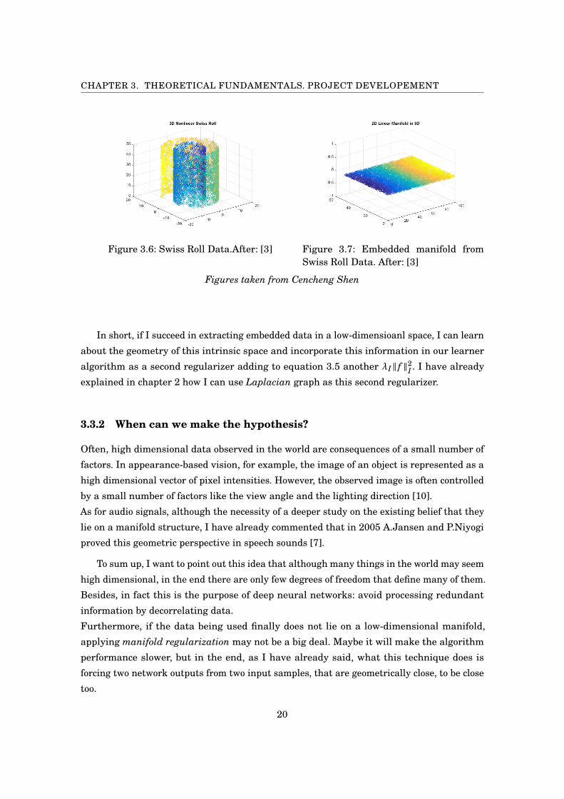
Figure 3.6: Swiss Roll Data.After: [3] Figure 3.7: Embedded manifold fromSwiss Roll Data. After: [3]

Figures taken from Cencheng Shen

In short, if I succeed in extracting embedded data in a low-dimensioanl space, I can learn

about the geometry of this intrinsic space and incorporate this information in our learner

algorithm as a second regularizer adding to equation 3.5 another λI‖ f ‖2I . I have already

explained in chapter 2 how I can use Laplacian graph as this second regularizer.

3.3.2 When can we make the hypothesis?

Often, high dimensional data observed in the world are consequences of a small number of

factors. In appearance-based vision, for example, the image of an object is represented as a

high dimensional vector of pixel intensities. However, the observed image is often controlled

by a small number of factors like the view angle and the lighting direction [10].

As for audio signals, although the necessity of a deeper study on the existing belief that they

lie on a manifold structure, I have already commented that in 2005 A.Jansen and P.Niyogi

proved this geometric perspective in speech sounds [7].

To sum up, I want to point out this idea that although many things in the world may seem

high dimensional, in the end there are only few degrees of freedom that define many of them.

Besides, in fact this is the purpose of deep neural networks: avoid processing redundant

information by decorrelating data.

Furthermore, if the data being used finally does not lie on a low-dimensional manifold,

applying manifold regularization may not be a big deal. Maybe it will make the algorithm

performance slower, but in the end, as I have already said, what this technique does is

forcing two network outputs from two input samples, that are geometrically close, to be close

too.

20

3.4. OBJECTIVE FUNCTION

3.4 Objective function

Gathering all what explained in chapter 2 and chapter 3, my final algorithm optimization

problem is defined as follows:

(3.6) f ∗ = argminf

1l

l∑i=1

( f (xi)− yi)2 +λ1

M∑j=1

w j2 + λ2

(u+ l)2 f T (x)Lf (x)

There are few things to comment about this equation.

To begin with, see that now the loss function is a mean of the labeled samples, that is why I

changed N (equal to u+ l) from equation 3.5 to l; Instead, as for the intrinsic regularizer I

am working with all the data, here I take into account either labeled and unlabeled samples.

In fact, for computing the graph I have to make N2 operations - linking or not linking each

sample withrespect all the others, that is why I divide the third part per (u+ l)2.

Furthermore,f(x) is the vector with all the network outputs (one for each training sample)

and L is the Laplacian graph.

Regarding the Laplacian graph, there is not a deep knowledge about which technique is

better for building a good graph depending on the data used. Right now, the solution to that

problem is empirical, and data scientists learn about the performances of each technique by

experience. A good graph construction will lead to a W with a balance between values from 0

to 1 (which would refer to the weights between linked samples) and 0, in reference to those

samples not linked.

In this work I compute just one graph and not the mean of few like what commented

in chapter 2, section 2.4 . Besides, I only compute the graph exploiting closeness between

points of a same class and do not take into consideration the penalty graph mentioned in

section 2.3 .

To sum up, recall that what I am doing with this graph construction, as it is said in

semi-supervised learning section, is forcing that if two input samples are geometrically close,

their network outputs should be close as well; but this idea is not new because it is the

purpose of any regularizer.

21

CH

AP

TE

R

4ALGORITHM. PROJECT DEVELOPMENT

The purpose of this chapter is , once we know all the theoretical background behind

the thesis, to describe technically what my algorithm consists on.

4.1 Algorithm

This work is based on a 1-hidden fully connected neural network. The hidden layer has

initially a fixed number of 10 neurons, and its input and output layers depend on the used

data. Firstly I used 4 datasets as benchmarks because they had already been proved to have

a manifold-based structure, so working with them was a good starting point. Two of them

are artificially created and the other two are real data. Then, having made sure that my

algorithm worked well, I wanted to prove the manifold assumption in real speech audio.

The experiments on this thesis are based on a binary classification problem, so that is

why I have used datasets of two classes, represented by labels −1 and 1. In the end, they all

have the same two-vector structure:

(4.1) X=

x1,1 x1,2 x1,3 . . . x1,n

x2,1 x2,2 x2,3 . . . x2,n

. . . . . . . . . . . . . .

xm,1 xm,2 xm,3 . . . xm,n

A matrix X , where the rows are the training samples and the columns, the features, namely,

the dimensions of the dataset in use. Before training, the algorithm normalizes the matrix

between values 0 and 1 to make sure it is working in a non-saturated region in relation to

23

CHAPTER 4. ALGORITHM. PROJECT DEVELOPMENT

the hyperbolic activation function, see again figure 3.3 from chapter 3.

(4.2) y=[

y1 y2 y3 . . . ym

]

The datasets are also defined by an output vector with the labels of the training samples.

This vector can only have 3 values: initially it only has −1’s and 1′s, but the algorithm

modifies it for each dataset by changing the value of an amount (specified in the GUI by the

user ) of random training samples to 0 in order to make them unlabeled (because 0 is the

only scalar at the same distance to label −1 than to 1)

Regarding the results, what I wanted was to obtain a lower missclassification error when

applying manifold regularization. As its name says, this error is the number of network

output labels different from the real ones according to the test samples.

With test I am referring to unseen data by the algorithm. If I used the same data that

my algorithm had used in the optimization process, obviously the performance would be

very good, because the network parameters would have been chosen for making the model

classify well when using this specific data. That is why in any machine learning problem, it

is essential to split always the data and leave one % only for computing the final error.

A standard training-test and labeled-unlabeled data ratios for getting quite good results are

test: 30%, training: 70% and labeled: 10% and unlabeled: 60% respectively. All of them are

thought to be with respect to the original data.

To compute this error I considered that any output network yi < 0 referred to label -1

and the ones > 0, to 1.

(4.3) error = #(sign( f (xtest)) 6= sign(ytest))m

x100

To sum up, this work comes down into two parts: the first one based on training the network

without applying MR and finding the optimum point for getting the minimum value of its

objective function and, hence, the minimum missclassification error. In this case λ will be

producing the only degree of freedom - see equation 3.5 in chapter 3. The second part is

based on taking advantage of the second degree of freedom gained by applying MR - see

equation 3.6 - to find any combination of values with which the algorithm performed with a

lower missclassification error.

24

4.2. SOFTWARE

Algorithm 1: 1-hidden fully connected layer for a binary classification problemData: [X , y] such that X is an mxn matrix with m samples and n features and y is an

mx1 vector with the labels of the m samples.begin

Import Data [X , y] Normalize X between [0,1] and y between [-0.9,0.9];Split Data 30% test | 70% training | % unlabeled. Set this % of y values to 0.;Define # hidden Layers;Compute Laplacian graph with Mellacci’s framework;Initialize weights from the uniform distribution according to Glorot and Bengio(2010);

Training;for n = 1 : epochs do

Compute f (x) by training the network forward.;Define f ∗, the optimization problem;Find d f ∗

w for each weight by back-propagation;Update weights: wl

i j = wli j −µ

d f ∗

dwljk

;

Test;Compute missclassification error: error = #(sign( f (xtest))6=sign(ytest))

m x100

4.2 Software

4.2.1 Matlab

In this work I have used Matlab programming language for building the ANN. After some

research, I realised that there was not a best choice but many options. It is true that right

now Python is the most used languages for deep learning because there are many software

frameworks written in Python such as Theano, Lasagne, Keras or TensorFlow... on the other

hand, there is MatCovNet, wich is a good framework written in Matlab, and few more in

other languages.

However, the will was not to use any framework as I wanted to compute a model from scratch

otherwise adding the manifold regularization part to these algorithms already written would

be quite tricky.

Another concern was the efficiency of the code; it is not the same writing fast code than

writing code fast. Maybe for the first purpose C/C++ would be a good language, but my goal

was to implement the easiest model in an easy environment to work. In addition Matlab is

the programming language I know best, so all these arguments made me choose Matlab for

building my ANN.

In the end, with Matlab I have been able to perform any setting I wanted and the final

25


code (based on Linear Algebra for making it faster) speed performance is considerably high.

4.2.2 Melacci’s Library

The only already-written framework I have used is one from Melacci for computing Laplacian

graph. The reason is that making a good graph means learning better the intrinsic geometry

of input data, and by using Melacci′s framework I obtained better algorithm performances

than when using mines in terms of performance speed and clearer results.

Besides, Melacci′s code allowed me to choose between different techniques for building the

graph, what gave me flexibility and dynamism for getting the optimum combination of

parameters in order to obtain good results, because as I have said before there is not a best

nor a worst technique for computing this graph.

4.2.3 Graphic User Interface

Following this idea, I made an easy GUI where I could choose different hyperparameters for

the proposed network like the input data, number of epochs (runs of the optimization loop -

forwardpropagation, backpropagation and weights update), the k neighbors of my graph W

. . .

As for results, this GUI shows the cost function behavior over number of epochs, also the

missclassification error behavior and its final value, all of them both when applying manifold

regularization and when not so that I can compare performances.

Figure 4.1: Graphic User Interface

26

4.2. SOFTWARE

4.2.4 Benchmark Datasets

Dataset Classes Dimension Samples Natureg50c 2 50 550 artificial

Digit1 2 241 1500 artificialUSPS 2 241 1500 real

BCI 2 117 400 real

Table 4.1: Benchmarks

Sets obtained from Oliver Chappelle at http://olivier.chapelle.cc/ssl-book/benchmarks.html

4.2.4.1 g50c

According to Oliver Chappele, "this data set was generated such that the cluster and manifold

assumptions hold" [15]. The class label of a point represents the Gaussian it was drawn

from. Finally, all dimensions are standardized, i.e. shifted and rescaled to zero-mean and

unit variance.

4.2.4.2 Digit1

This dataset consists of 1500 artificial writing images of digit "1" developed by Matthias Hein

(Hein and Audibert, 2005). Then, a set of transformations were applied to each image, such

as rescaling, adding noise, permutation... In the end, although each image has 241 features,

initially the dimensions of the input, this set of transformations make them finally have only

five degrees of freedom, so it made sense to do the manifold assumption to this dataset.

4.2.4.3 USPS

The dataset refers to numeric data obtained from the scanning of handwritten digits from

envelopes by the U.S. Postal Service. The original scanned digits are binary and of different

sizes and orientations; the images here have been deslanted and size normalized, resulting

in 16 x 16 grayscale images (Le Cun et al., 1990).

Again, like with digit1 dataset, Oliver Chappelle applied some transformations to make the

data obscurer.

4.2.4.4 BCI

BCI are the Acronym for Brain Computer Inter f ace, which is a direct communication

pathway between an enhanced or wired brain and an external device. This dataset was

obtained after 400 trials of a person who had to imagine movements with both the left hand

27


(label −1) and the right one (label 1). The electric signals were recorded by 39 electrodes (in

each trial) and represented by a regressive model of order 3, so that is why finally each trial

is defined by 117 parameters.

4.2.5 Real Speech Sound Dataset

A case of high interest is the network training with real dataset NIST-SRE-00. This Speaker

Recognition Evaluation dataset was developed by the National Institute of Standards and

Technology. Each sample represents a native-english human voice by 11 parameters and,

although the labels were initially 0 for man and 1 for human, I changed the 0 one for -1

to make this data feasible to train with the proposed NN. This set consists on more than

300000 samples, but I make three subsets of different length because I cannot work with

such amount of points and in order to make the results and conclusions more robust.

Dataset Classes Dimension Samplesspeech data 2 11 501

speech data 2 2 11 2001speech data 3 2 11 8001

Table 4.2: Real speech data

This dataset was provided by Marc Palet

28

CH

AP

TE

R

5RESULTS

This section presents and discuss the results of the several experiments carried out. In

sections 5.1 and 5.2 I present the results for training with different datasets a 1-hidden fully

connected layer NN with 10 hidden neurons. The proposed NN is trained with 70% of the

samples, and the final error is computed with the rest. In all the experiments 60% of the

samples are unlabeled, and the Heat Kernel value is 1. The majority of the experiments are

carried out with 40 nearest neighbors k and a learning rate of 0.01. The whole setting for

each experiment is provided in the appendix section.

5.1 Benchmarks

Dataset errornonMR errorMRg50c 35.15 6.667

digit1 6.889 6.444USPS 10.22 9.556BCI 44.17 40.83

Table 5.1: Missclassification errors for benchmark datasets.

The errors are displayed in %; all the other hyperparameters settings are provided in theappendix section.

What we can see is that manifold regularization improves the proposed NN performance

in all the cases but with different intensity; regarding the benchmarks, this was expected

29

CHAPTER 5. RESULTS

because I already knew that data was lying on a submanifold structure. The results are quite

easy to justify for g50c, digit1 and USPS: the first one was artificially created making sure

the data lied on a manifold (that is why the improvement gained when applying MR has

been the biggest one in comparison to the results with other datasets) and the other two are

images which, as I already said, are proved to depend on few degrees of freedom, so that is

why we can make the manifold assumption.

Regarding the results of BCI, although the results are not as consistent as the ones obtained

with the other datasets because this one have only 400 samples, we can agree MR has also

improved the algorithm performance. This is less obvious, but it seems plausible that the

signals captured by an EEG have rather few degrees of freedom [20]. Besides, In 1963 Lorenz

demonstrated the possibility that the unpredictable or chaotic behavior observed in any

infinite-dimensional system might be caused by a three-dimensional dynamical system, and

EEG signals are considered so.

5.2 Speech Audio Dataset

Dataset errornonMR errorMRspeech data 1 13.33 11.33speech data 2 7.833 7.5speech data 3 7.75 7.542

Table 5.2: Missclassification errors for speech audio datasets.

The errors are displayed in %; all the other hyperparameters settings are provided in theappendix section.

In regards real speech sound data, we can see that MR works too, proving like A.Jansen

and P.Niyogi did in 2005 that speech signals are defined by few degrees of freedom [7].

Starting from the idea that the acoustic analysis of the vocal tract resonator can be reduced

to the tractable problem of concatenated uniform acoustic tubes with several approximations

[18], the dimension of the manifold would be determined by the number of tubes that compose

the vocal filter and the number of independent parameters that configure them.

However, looking at table 4.2 we can see an unexpected behavior: the more data it is

trained, the more the algorithm learns, so theoretically the lower the final error is. Here,

instead, we can see how although speech data 3 has 4 times more data than speech data

2, the algorithm performs a little bit better training the second one. Furthermore, this only

happens when I apply MR; when applying only standard regularization, the behavior is

30

5.3. STANDARD REGULARIZATION PLUS MANIFOLD

more logical. The more data, the lower the missclassification error, but with an exponential

decay.

Taking into account the insignificant increase in the error and the limitations and simplicity

of my algorithm, I strongly belief I might have not got to the optimum point when considering

the manifold assumption, so I will not give that much weight.

5.3 Standard Regularization Plus Manifold

Another interesting result to point out is the fact that, with any dataset, my algorithm per-

formance has improved when I have applied both regularizers and not just the manifold one.

It is a combination of both ambient and intrinsic regularizers which makes the performance

improve.

The conclusion I extract from this is that although both techniques are regularizers with

the same purpose to make the learning function smooth, they might influence the network

performance in different ways. Let’s see this:

As an example, let’s take a look to figure 3.5 from chapter 3 again,

Figure 5.1: Semi Supervised Learning.

What MR does is making sure that if two inputs points are geometrically close, their

respective outputs must be close too. Looking at the image, this intrinsic regularizer would

be the responsible of gathering the network outputs discriminatively forming the two class

groups. However, this does not make the decision boundary smooth; maybe by applying MR

we classify well our training samples but what if the decision boundary function is still a

high-order polynomial varying so much? For unseen data, the classifier may still perform

poorly. It is here where standard regularization plays its role making this function smoother.

31

CHAPTER 5. RESULTS

5.4 Deep Learning

Another study I carried out is the influence of MR in a deep learning context. I trained g50c

dataset with, now, different hidden layer settings, and in every experiment I could find a

good combination of hyperparameters with which the classifier performed as well as when

training with the initial 1 hidden layer of 10 neurons, but never better. Bearing in mind the

simplicity of the experiment - the hidden layers settings had from two to three layers and

the dataset used was artificial and with a very simple architecture - I cannot extract robust

conclusions from this.

The relation between hidden layers and algorithm performance depends on the dataset

structure and the samples. The more complex and the bigger the dataset is, the more

non-linear information can be extracted; so it seems normal that with an artificial and

simple dataset of 550 samples like g50c is, we can not see any performance improvement

increasing the number of hidden layers. However, the interesting thing is that I could see

little improvements when I trained the NN without manifold regularization, but not when

applying it. Although this idea should also be further worked, it is quite obvious that with

proper dataset, I would get interesting results.

From the other part, what I could surely conclude from this study is that the fact that

increasing the amount of layers do not worsen the performance is already a proof that the

regularization is working, because dealing with more hidden layers means having more

network weights and a potential higher-order polynomial.

5.5 g241c

The proposed network was also trained with data which had not a low-dimensional manifold

structure in order to check if MR then worsens or not the performance. For this goal I

used g241c dataset, also provided by Oliver Chapelle. According to him, this datasaet " was

generated such that the cluster assumption holds, i.e. the classes correspond to clusters, but

the manifold assumption does not".

Surprisingly, I did not get the results expected by training the network with g241c. I

could not find any point at which applying also MR at least made me obtain the same results

as if I applied only standard regularization. It always worsened the algorithm performance.

Appealing to the possible argument exposed in section 5.3, as both regularizers finally don’t

do exactly the same, it might be normal not to expect the same final error when applying

MR. However, this is an open aspect to be investigated in future research.

32

5.6. COMPUTATIONAL COST

5.6 Computational Cost

It is obvious that applying manifold regularization implies a worsening in the computational

complexity of the algorithm. It can be seen in two aspects: When initially initializing all

the link weights for the Laplacian graph and when back-propagating k neighbors for each

feature vector, see again equations 3.3 and 3.6 and recall f ∗ is the optimization problem,

namely, the cost function C with the constrains of the regularizers.

This complexity addition is manifested in an increase of the performance timing. I

computed the timings for the NN performance when training digit1, USPS and speech data

3 because they are the datasets with more features (the first two), and more samples (speech

dataset), the two things which Laplacian graph depends on. The results are the following

ones:

Dataset timenonMR timeMRdigit1 3’ 03" 3’ 27"USPS 4’ 31" 6’ 01"

speech data 3 3’ 12" 5’ 16"

Table 5.3: Algorithm performance timings.

This timings have been computed with the same settings used in sections 5.1 and 5.2.

In this table, we can see how the presented algorithm takes a longer time when it applies

MR. Although the complexity addition may not seem relevant in these experiments, with

really huge and complex datasets the difference between performance timings may reach

tens of hours like in [22]. However, this complexity is only seem in the training part, as in

the test part the algorithm only trains forward with the test samples and the optimized

network weights.

33

CH

AP

TE

R

6CONCLUSIONS AND FURTHER WORK

6.1 Conclusions

This work has presented a technique for exploiting the intrinsic geometry of the input

datasets in order to make 1-hidden fully connected layer neural network generalize better. In

has been demonstrated how projecting the data on the egeinvectors of the Laplacian graph

results to a feature map with local distances preserved from which training data can be

worked easily.

The algorithm performance is evaluated with benchmark datasets and is compared to that

obtained when the technique in question is not applied. Results clearly show the improvement

in performance of the algorithm applying MR, with missclassification error drops ranging

2 to 7.5%, and reaching 80% in a particular case, when using the synthetic datset g50c.

Besides, the network is trained with a real speech dataset proving the assumption speech

data lie on a low-dimensional manifold. An explanation to this statement is presented. If

we look the performance algorithm from a computational perspective, this work shows the

increase of complexity when the technique in question is applied.

In this thesis, it is also proved the improvement of the algorithm performance when

applying both ambient and intrinsic regularizers rather than only one. A possible explanation

to that result is presented. It is also introduced a study of the technique applied in a NN

with different amount of hidden layer, left as an open aspect to be worked in future research.

The consistent gains in the algorithm performance applying manifold reuglarization

35

CHAPTER 6. CONCLUSIONS AND FURTHER WORK

might suggest this thesis as a proof-of-concept for more advanced research in the topic.

6.2 Future Work

In accordance to the results presented in the thesis, three further research topics should be

mentioned.

The first one would be understanding and exploiting better the idea that the algorithm

gains in performance when applying both regularizers. The results of this work suggests

that, although their goal is the same as of any regularizer, their influence in the algorithm

performance might be different.

The second main topic would be exploiting better the hierarchical structure of a deep neural

network, with more than three hidden layers and hundreds of hidden units each, training

the DNN with more complex datasets.

Last but not least, once having made the proof-of-concept of the improvement in the algo-

rithm generalization when applying this technique, future research may focus on comparing

this regularizer with the others for different datasets because, as it has been mentioned

before, much of the understanding of machine learning algorithms is obtained from empirical

experiments due to the absence of an optimal algorithm for all the datasets.

36

AP

PE

ND

IX

AAPPENDIX A

Dataset µnonMR µMR epochs %unlabeled k-NN neighbors Heat Kernel λ λMR λ2MR errornonMR errorMRg50c 0.01 0.01 15000 60 40 1 0.002 0.02 100000 35.15 6.667

digit1 0.01 0.01 20000 60 40 1 0.2 0.002 1000 6.889 6.444USPS 0.01 0.01 30000 60 40 1 0.002 0.002 100 9.778 9.556BCI 0.005 0.005 50000 60 40 1 0.002 0.02 1000 44.17 40.83

speech data 1 0.01 0.01 5000 60 40 1 0.2 0.02 100000 13.33 11.33speech data 2 0.01 0.01 5000 60 40 1 0.02 0.2 100000 7.833 7.5speech data 3 0.01 0.01 10000 60 250 1 0.2 0.01 2000000 7.75 7.542

Table A.1: Full hyperparameters network setting for each dataset.

µ’s control the proportion of gradient descent that influences the weights update -see equation3.4 in Chapter 3. Epochs determine the number of loops in which feed-forward training,backpropagating and weights update are run. The 6th and 7th column refer to the techniqueapplied with Melacci’s code for building the graph matrix. The missclassification error hasbeen computed with the 30% of initial data, reserved for the test part.

Hidden Layers µnonMR µMR epochs %unlabeled k-NN neighbors Heat Kernel λ λMR λ2MR errorMR[5] 0.01 0.01 10000 60 40 1 0.002 0.02 100000 6.667

[1010] 0.01 0.01 15000 60 40 1 0.02 0.02 100000 6.667[105] 0.01 0.01 30000 60 40 1 0.002 0.02 100000 6.667[55] 0.01 0.01 15000 60 40 1 0.002 0.02 300000 6.667

[101010] 0.01 0.01 8000 60 40 1 0.002 0.02 100000 6.667[1055] 0.01 0.01 30000 60 40 1 0.002 0.01 250000 6.667

Table A.2: g50c trained with different hidden layer settings.

The first column shows the hidden layer settings of each train. The format is a vector withcomponents as hidden layers and their values, the number of neurons at them.

37

AP

PE

ND

IX

BGLOSSARY

−NN : NeuralNetwork

−DNN : DeepNeuralNetwork

−SSL : Semi−SupervisedLearning

− ASR : AutomaticSpeechRecognition

−SV M : SupportV ectorMachine

−RLS : RegularizedLeastSquare

−EMR : EnsembleMani f oldRegularization

−MRE : MeanSquaredError

−GUI : GraphicUserInter f ace

−MR : Mani f oldRegularization

−EEG : Electroencephalogram

39

BIBLIOGRAPHY

[1] M. BELKIN AND P. NIYOGI, Laplacian Eigenmaps and Spectral Techniques for Embed-

ding and Clustering, 2001.

[2] C. X. L. Y. BO GENG, DACHENG TAO AND X.-S. HUA, Ensemble Manifold Regulariza-

tion, 2009.

[3] J. T. V. CENCHENG SHEN AND C. E. PRIEBE, Manifold Matching using Shortest-Path

Distance and Joint Neighborhood Selection, Elsevier, 2016.

[4] G. CYBENKO, Approximation by superpositions of a sigmoidal function, Mathematics of

control, signals and systems 2.4, 1989.

[5] A. ERRITY AND J. MCKENNA, An Investigation of Manifold Learning for Speech Analy-

sis, INTERSPEECH, 2006.

[6] L. FAUSETT, Fundamentals of Neural Networks: Architectures, Algorithms And Appli-

cations, Pearson, 1993.

[7] A. JANSEN AND P.NIYOGI, A Geometric Perspective on Speech Sounds, 2005.

[8] R. C. JASON WESTON, FRÉDÉRIC RATLE, Deep learning via semi-supervised embedding,

International Conference on Machine Learning, Helsinki, Finland, 2008.

[9] X. LU AND J. DANG, Vowel Production Manifold: Intrinsic Factor Analysis of Vowel

Articulation, IEEE Transactions on Audio Speech and Language Processing, 2010.

[10] A. K. J. MARTIN H. C. LAW, Incremental Nonlinear Dimensionality Reduction By

Manifold Learning, IEEE.

[11] P. N. MIKHAIL BELKIN AND V. SINDHWANI, Manifold Regularization: A Geometric

Framework for Learning from Examples, Journal of Machine Learning Research,

2004.

41

BIBLIOGRAPHY

[12] V. S. MIKHAIL BELKIN AND P. NIYOGI, Beyond the point cloud: from transductive to

semi-supervised learning, ICML ’05 Proceedings of the 22nd international conference

on Machine, 2005.

[13] M. A. NIELSEN, Neural Networks and Deep Learning, Determination Press, 2015.

[14] P. NIYOGI AND M. BELKIN, Semi-Supervised Learning on Riemannian Manifolds,

Kluwer Academic Publishers, 2004.

[15] A. Z. OLIVIER CHAPELLE, BERNHARD SCHOLKOPF, Semi-Supervised Learning, The

MIT Press, 2006.

[16] V. S. PARTHA NIYOGI AND M. BELKIN, On Manifold Regularization, 2004.

[17] P.J.WERBOS, Beyond Regression: New Tools for Prediction and Analysis in the Behav-

ioral Sciences., 1975.

[18] P.NIYOGI AND A. JANSEN, Intrinsic Fourier Analysis on the Manifold of Speech Sounds,

IEEE, 2006.

[19] L. ROSASCO, Manifold Regularization, Lecture in Statistical Learning Theory and

Applications, 2010.

[20] J. RÖSCHKE AND E. BASAR, Correlation Dimensions in Various Parts of Cat and Human

Brain in Different States, Springer Berlin Heidelberg, 1990.

[21] J. SNYMAN, Practical mathematical optimization: an introduction to basic optimization

theory and classical and new gradient-based algorithms, Vol. 97. Springer Science

[22] V. S. TOMAR AND R. C. ROSE, Manifold Regularized Deep Neural Networks, INTER-

SPEECH, 2014.

[23] S.-F. C. WEI LIU, JUNFENG HE, Large Graph Construction for Scalable Semi-

Supervised Learning, International Conference on Machine Learning, 2010.

[24] H. WU, Global stability analysis of a general class of discontinuous neural networks

with linear growth activation functions., Information Sciences, 2009.

[25] G. B. O. YAN LECUN, LEON BOTTOU AND K. R. MULLER, Efficient Backprop., 1975.

42

Study and implementation of manifold regularization ...

Documents

Transcript of Study and implementation of manifold regularization ...