Cohomology of real Grassmann manifold and KP flow
47
COHOMOLOGY OF REAL GRASSMANN MANIFOLD AND KP FLOW LUIS CASIAN AND YUJI KODAMA * Abstract. We consider a realization of the real Grassmann manifold Gr(k, n) based on a par- ticular flow defined by the corresponding (singular) solution of the KP equation. Then we show that the KP flow can provide an explicit and simple construction of the incidence graph for the integral cohomology of Gr(k, n). It turns out that there are two types of graphs, one for the trivial coefficients and other for the twisted coefficients, and they correspond to the homology groups of the orientable and non-orientable cases of Gr(k, n) via the Poincar´ e-Lefschetz duality. We also derive an explicit formula of the Poincar´ e polynomial for Gr(k, n) and show that the Poincar´ e polynomial is also related to the number of points on a suitable version of Gr(k, n) over a finite field Fq with q being a power of a prime. In particular, we find that the number of Fq points on Gr(k, n) can be computed by counting the number of singularities along the KP flow. Contents 1. Introduction 2 2. The real Grassmann manifold Gr(k,n) 8 2.1. The Schubert decomposition 8 2.2. The Pl¨ ucker embedding and the moment polytope 10 3. The KP flow on Gr(k,n) 11 3.1. The KP flow on the moment polytope 11 3.2. The KP equation and the Toda lattice 13 3.3. Remark on the Toda lattice description 15 4. The set S (k) n and the graph G (k) n 16 4.1. The decomposition of S (k) n 18 4.2. The decomposition of Gr(k,n) 19 5. The graph G(k,n) 21 5.1. The signed Schubert cells 22 6. Proof of the main Theorem for the incidence graph 25 6.1. The case of Gr(2, 4) 25 6.2. Some standard notation 26 6.3. Connection of the cohomology of G/B with Hecke algebra operators 27 6.4. The edge in the incidence graph associated to B w ∪B siw 28 6.5. K-equivariant local systems on G/B and their Toda signs 28 6.6. Computation of the signs (σ, L) 29 6.7. Proof of Theorem 31 7. The Poincar´ e polynomials 34 7.1. The polynomials P * (k,n) (t) 34 7.2. The polynomials P (k,n) (t) 36 8. The F q points on Gr(k,n) and the Poincar´ e polynomials 39 8.1. The q-weighted Schubert cells 39 * Partially supported by NSF grant DMS0806219. arXiv:1011.2134v1 [math.AG] 9 Nov 2010
-
Upload
independent -
Category
Documents
-
view
0 -
download
0
Transcript of Cohomology of real Grassmann manifold and KP flow

COHOMOLOGY OF REAL GRASSMANN MANIFOLD AND KP FLOW
LUIS CASIAN AND YUJI KODAMA∗
Abstract. We consider a realization of the real Grassmann manifold Gr(k, n) based on a par-
ticular flow defined by the corresponding (singular) solution of the KP equation. Then we showthat the KP flow can provide an explicit and simple construction of the incidence graph for the
integral cohomology of Gr(k, n). It turns out that there are two types of graphs, one for the trivial
coefficients and other for the twisted coefficients, and they correspond to the homology groups ofthe orientable and non-orientable cases of Gr(k, n) via the Poincare-Lefschetz duality. We also
derive an explicit formula of the Poincare polynomial for Gr(k, n) and show that the Poincare
polynomial is also related to the number of points on a suitable version of Gr(k, n) over a finitefield Fq with q being a power of a prime. In particular, we find that the number of Fq points on
Gr(k, n) can be computed by counting the number of singularities along the KP flow.
Contents
1. Introduction 22. The real Grassmann manifold Gr(k, n) 82.1. The Schubert decomposition 82.2. The Plucker embedding and the moment polytope 103. The KP flow on Gr(k, n) 113.1. The KP flow on the moment polytope 113.2. The KP equation and the Toda lattice 133.3. Remark on the Toda lattice description 15
4. The set S(k)n and the graph G(k)
n 16
4.1. The decomposition of S(k)n 18
4.2. The decomposition of Gr(k, n) 195. The graph G(k, n) 215.1. The signed Schubert cells 226. Proof of the main Theorem for the incidence graph 256.1. The case of Gr(2, 4) 256.2. Some standard notation 266.3. Connection of the cohomology of G/B with Hecke algebra operators 276.4. The edge in the incidence graph associated to Bw ∪ Bsiw 286.5. K-equivariant local systems on G/B and their Toda signs 286.6. Computation of the signs ε(σ,L) 296.7. Proof of Theorem 317. The Poincare polynomials 347.1. The polynomials P ∗(k,n)(t) 34
7.2. The polynomials P(k,n)(t) 368. The Fq points on Gr(k, n) and the Poincare polynomials 398.1. The q-weighted Schubert cells 39
∗Partially supported by NSF grant DMS0806219.
arX
iv:1
011.
2134
v1 [
mat
h.A
G]
9 N
ov 2
010

2 LUIS CASIAN AND YUJI KODAMA∗
8.2. The number of Fq-points on Gr(k, n) 438.3. Frobenius eigenvalues calculation 46References 46
1. Introduction
This paper attempts to extract the topology of real Grassmannians based on a realization of themanifolds related to the KP hierarchy. As in the case of the real flag manifolds discussed in [8] usingthe Toda lattice hierarchy, we here show that the KP equation can be used to obtain similar resultsfor the real Grassmannians.
The KP equation is a two-dimensional extension of the well-known KdV equation, and it wasintroduced by Kadomtsev and Petviashvili in 1970 to study the stability of one KdV soliton underthe influence of weak two-dimensional perturbations [18]. The equation provides also a model todescribe a two-dimensional shallow water wave phenomena (see for example [1, 27, 20, 11]. The KPequation is a dispersive wave equation for the scaler function u = u(x, y, t) with spatial variables(x, y) and time variable t, and is given by
∂
∂x
(−4
∂u
∂t+ 6u
∂u
∂x+∂3u
∂x3
)+ 3
∂2u
∂y2= 0.
We write the solution in the form
u(x, y, t) = 2∂2
∂x2ln τ(x, y, t),
where the function τ is called the tau function of the KP equation [26, 25]. It is also well-knownthat some of the exact solutions can be written in the Wronskian determinant form (see for example[15]),
(1.1) τ = Wr(f1, f2, . . . , fk) :=
∣∣∣∣∣∣∣∣∣f1 f2 · · · fkf ′1 f ′2 · · · f ′k...
. . .. . .
...
f(k−1)1 f
(k−1)2 · · · f
(k−1)k
∣∣∣∣∣∣∣∣∣ ,where f
(l)j := ∂lfj/∂x
l, and each of the functions {fi(x, y, t) : i = 1, 2, . . . , k} satisfies the simplelinear equations,
∂fi∂y
=∂2fi∂x2
,∂fi∂t
=∂3fi∂x3
.
We then take the following finite dimensional solutions, (i.e. finite Fourie series),
fi =n∑j=1
ai,jEj , with Ej := exp(λjx+ λ2
jy + λ3j t),
where A := (ai,j) is an k × n real matrix of rank k, and λj ’s are real and distinct numbers, say
λ1 < λ2 < · · · < λn.
Since λj ’s are all distinct, the set of exponential functions {Ej : j = 1, . . . , n} is linearly independentand forms a basis of Rn. Then the set of {fi : i = 1, . . . , k} defines a k-dimensional subspace in Rn.This implies that each solution defined by the τ -function (1.1) can be characterized by the A-matrix,hence the solution parametrizes a point of the real Grassmannian. Note here that the Grassmanniandenoted by Gr(k, n,R) can be described as
Gr(k, n,R) = GLk(R) \Mk×n(R),

COHOMOLOGY OF REAL GRASSMANNIAN AND KP FLOW 3
where Mk×n(R) is the set of all k× n matrices of rank k, and GLk(R) is the general linear group ofk × k matrices. We then expect that some particular solutions of the KP equation contain certaininformation on the cohomology of Gr(k, n,R). This is our main motivation for the present study. Inthe previous paper [8], we found the similar results for the case of real flag variety using the Todalattice equation.
Let us explain how some solutions contain information of the cohomology of Gr(k, n,R) by takingsimple example with k = 1 and n = 4. That is, we recover the cohomology of real variety RP 3 ∼=Gr(1, 4,R) from a KP flow. We consider the τ -function in the form,
(1.2) τ = ε1E1 + ε2E2 + ε3E3 + ε4E4,
where εj are arbitrary non-zero real constants. Since |εj | can be absorbed in the exponential term,we only consider their signs, and here we assume εj ∈ {±} (which we refer to as KP signs). Letus consider the case with the specific signs (ε1, . . . , ε4) = (+,−,−,+). Using simple asymptoticargument, one can easily find that each Ej(x, y, t) becomes dominant in certain region of the xy-plane for a fixed t. Figure 1 illustrates the contour plots of the solution u(x, y, t) at t > 0 and t < 0.Each region marked by the number (i) indicates the dominant exponential Ei, and at the boundaryof the region, the τ -function can be expressed by two exponential functions Ei and Ej (which isdominant in the adjacent region), i.e. writing Ei = eθi with θi = λix+ λ2
i y + λ3i t,
τ ≈ εiEi + εj Ej
= ±2e12 (θi+θj)
{cosh 1
2 (θi − θj) if εiεj = +,
sinh 12 (θi − θj) if εiεj = −.
Then at the boundary, the solution has the following form depending on the sign εiεj ,
u =1
2(λi − λj)2
{sech2 1
2 (θi − θj) if εiεj = +,
csch2 12 (θi − θj) if εiεj = −.
In Figure 1, the sech-part (regular) of the solution is shown by the dark colored contour, and thecsch-part (singular) is shown in the light colored contour. We construct a polytope whose verticesare labeled by the dominant exponentials. The polytope for our example is a tetrahedron as shownin Figure 1. We then consider a KP flow choosing a particular parameter set (x, y, t), so that theflow is passing near the edges of the polytope. The flow might be expressed as a graph,
(1.3) (1) −→ (2) =⇒ (3) −→ (4),
where → shows the singular flow, and the ⇒ shows the regular one. It is then interesting to notethat the graph is the incidence graph of the real projective space RP 3, if the arrows are identifiedas the coboundary operators and their incidence numbers are assigned as 0 for → and ±2 for ⇒.
This kind of graph, exemplified by graph (1.3), was introduced in [8] in an initial attempt tocompute the number of connected components carved up by the zero divisors of the τ -function, i.e.τi = 0 for some i, within a moment polytope for the Toda flow. In the case of the KP flow Figure 1shows that this graph does not contain enough information to attempt to do this (one would haveto connect (1) and (4) with an edge ⇒). Still the main results in [8], which then motivated thispaper, were the result of an observation that such a graph, exclusively defined in terms of the flowcrossing or not crossing singularities, agrees, in the case of the Toda flow, with the incidence graphof real flag manifolds. The results in this paper extend this type of results to the KP flow.
As in [8] a polynomial can be defined by counting singularities crossed and taking an alternatingsum. In this case we obtain 1− q2, and now q(q2−1), with q a power of a prime number, counts thenumber of points over a finite field, Fq, of a variety closely related to Gr(1, 4,R) . This is explainedin more detail below and generalized. The cohomology calculation can be thought of as actually

4 LUIS CASIAN AND YUJI KODAMA∗
-100 -50 0 50 100-100
-50
0
50
100
-100 -50 0 50 100-100
-50
0
50
100
(1) (4)
(3)
(2)
(1)
(2)
(3)
(4)
(1)
(2)
(3)
(4)
Figure 1. The contour plot of the KP solution with the τ -function given by (1.2).The signs are chosen as (ε1, . . . , ε4) = (+,−,−,+). In the left two figures, thenumber (i) of each region represents the dominant exponential Ei, and the dark(light) colored contour shows the regular (singular) part of the solution. The leftfigure shows the contour plot of the solution at t = −5 and the middle one is at t = 5.The tetrahedron in the figures indicates as a dual graph of the solution pattern,that is, the vertices of the polytope are labeled by the dominant exponentials. Thedirected curve in the right figure shows a flow of the KP equation, and this flowblows up twice by crossing the boundary between the regions with different signs,which corresponds to τ = 0.
taking place over a field of positive characteristic (etale cohomology) so that these qi, i countingsingularties crossed, appear as Frobenius eigenvalues in cohomology.
One should note in the graph that the numbers (i) representing the dominant exponential Eilabel the Schubert cells of the variety RP 3, i.e.
RP 3 = X(1) tX(2) tX(3) tX(4),
where X(i) is the Schubert cell of dimension i− 1 (see Section 2). In this paper, we intend to showthat this view of the KP flow can be used to construct the incidence graph of the real Grassmannvariety Gr(k, n,R) in general.
We simply denote Gr(k, n,R) by Gr(k, n). Here we present an overview of the paper. Let Sn bethe symmetric group with the simple reflections sj for j = 1, . . . , n − 1, and Pk be the parabolicsubgroup of Sn generated by {sj : j = 1, . . . , n, j 6= k}. We then have the Schubert decompositionof Gr(k, n),
Gr(k, n) =⊔
w∈S(k)n
Xw,
where S(k)n is the set of minimal coset representatives of Sn/Pk ([2], see also Section 4). In this
paper, we are interested in the integral cohomology of Gr(k, n) which we find by constructing thecorresponding incidence graph (Section 5). The co-chain complex may be expressed as follows: Theset of the co-chains are defined by
C∗ =
k(n−k)⊕j=0
Cj , with Cj =⊕j=l(w)
Z〈w〉,
where l(w) is the length of w ∈ S(k)n , and 〈w〉 := Xw, the Schubert cycle. For each j, we define an
operator δj : Cj → Cj+1 in the form, for 〈w〉 ∈ Cj and 〈w′〉 ∈ Cj+1,
δj〈w〉 =∑
l(w′)=l(w)+1
[w;w′] 〈w′〉.

COHOMOLOGY OF REAL GRASSMANNIAN AND KP FLOW 5
where w′ = siw for all si with l(siw) = l(w) + 1. The coefficient [w,w′] takes the value either 0or ±2 ([19], see also Section 5). Then we define a graph G(k, n), which can be described along the
KP flow, and which consists of the vertices given by 〈w〉 for w ∈ S(k)n and the edges given by the
(double) arrows between 〈w〉 and 〈w′〉 when [w,w′] 6= 0, that is, there is no blow up. For example,in the case of Gr(1, 4) ∼= RP 3, we have C∗ = Z[〈e〉]⊕Z[〈s1〉]⊕Z[〈s2s1〉]⊕Z[〈s3s2s1〉], and the graphG(1, 4) is given by
〈e〉 −→ 〈s1〉 =⇒ 〈s2s1〉 −→ 〈s3s2s1〉.This graph is the incidence graph for RP 3 when we assign the coefficients as [e; s1] = 0, [s1; s2s1] = ±2and [s2s1; s3s2s1] = 0 (cf. (1.3)). This can be extended to the general case, and in Section 6, weprove the main theorem,
Theorem 1.1. The graph G(k, n) is the incidence graph for the real Grassmannian Gr(k, n).
The proof of this theorem is based on [9] and a simplified description of these results for thereal split case which are described in terms of the Toda lattice in [8]; finally an adaptation of [8] sothat incidence graphs are expressed exclusively in terms of the KP flow, which, it turns out, furthersimplifies the case of real Grassmanians allowing easy explicit calculation of Betti numbers.
Based on the graph G(k, n), we then derive explicit formulas for Betti numbers of real Grass-manians, and discuss relations of these Betti numbers to the number of points over a finite fieldof certain related varieties. For this computation, we first replace the real Grassmanian manifoldGr(k, n) with a complex manifold, a Zariski open subset Gr(k, n)C ⊂ Gr(k, n,C) with the samehomotopy type (see subsection 8.2 for the details). The variety Gr(k, n)C can be considered overother fields, for example, a finite field Fq with q elements. The number of Fq points i.e. the numberof points on Gr(k, n)Fq , is given by a polynomial of q denoted by |Gr(k, n)Fq |. In section 8, we showthat the polynomial |Gr(k, n)Fq | is related to the Poincare polynomial of the real variety Gr(k, n).The cohomology of Gr(k, n) is much more complicated than the cohomology of the complex varietyGr(k, n,C), since it involves torsion. However we find that, the Betti numbers of Gr(k, n,C) andGr(k′, n′) for some (k′, n′) determined from (k, n), agree after taking into account a change in de-grees. Recall that the Poincar’e polynomial of the complex variety Gr(k, n,C), denoted by PC
(k,n)(t),
is simply obtained by the number of Fq points, |Gr(k, n,C)|. That is, we have
PC(k,n)(t) = |Gr(k, n,Fq)|q=t2 =
∑w∈S(k)
n
t2l(w) =
[nk
]t2,
Here the polynomial
[nk
]q
is a q-analog of the binomial coefficient(nk
)(see section 2).
The simplest example is the case of Gr(1, 2) ∼= RP 1 which is a circle S1 and can be described withan equation x2 + y2 = 1. The number of Fq points of Gr(1, 2), that is the number of the solutions ofx2 + y2 = 1 for x, y ∈ Fq, is q− 1 (see Remark 1.1 below). We thus have a polynomial in q, namely,
|Gr(1, 2)Fq | = q − 1,
and we note that this gives the Betti numbers βk as coefficients of (−1)1−jqj , j = 0, 1, in the poly-
nomial, i.e. |Gr(1, 2)Fq | =n∑j=0
(−1)n−jβjqj . Namely the Poincare polynomial for Gr(1, 2) denoted
by P(1,2)(t) is given by
P(1,2)(t) =1∑j=0
βjtj = 1 + t.
Remark 1.1. In fact, there are two formulas for the number of points of x2+y2 = 1 over Fq dependingon q (q not a power of 2). For instance over F3 we have |S1(F3)| = q + 1 = 4; however over F5

6 LUIS CASIAN AND YUJI KODAMA∗
there |S1; (F5)| = q − 1 = 4. By extending F3 to F32 (adding√−1), the number of Fq points with
q = 32 = 9 becomes q − 1. We assume in this paper√−1 ∈ Fq.
In a similar computation (see the subsection 8.2), we obtain the number of Fq points of RP 3 ∼=Gr(1, 4) as
|Gr(1, 4)Fq | = q(q2 − 1).
The Poincare polynomial for this case is given by
P(1,4)(t) = 1 + t3,
and the relation with |Gr(1, 4)Fq | is not obvious, but we note that the replacement q2 − 1 to 1 + t3
gives the relation between those polynomials. It turns out that the similar replacement can be donefor the general cases of Gr(2j + 1, 2m) (see the subsection 8.1).
A more interesting example is Gr(2, 4)which is discussed in Example 2.2 below. The polynomialthat results in this case is q2(1 + q2) giving the number of Fq points on Gr(2, 4). Notice that thepolynomial 1 + q2 is also Gr(1, 2,Fq2) i.e., we have
|Gr(2, 4)Fq | = q2|Gr(1, 2,Fq2)| = q2PC(1,2)(q) = q2
[21
]q2.
The Poincare polynomial is obtained from 1 + q2 by replacing q with t2, and is related to PC(1,2)(q)
i.e.P(2,4)(t) = PC
(1,2)(t2) = 1 + t4.
Remark 1.2. This relation of the Poincar’e polynomials suggests that the ring of polynomials forthe real cohomology for Gr(2, 4) be expressed by
H∗(Gr(2, 4),R) ∼=R[p]
{p2},
where p is the Pontrjagin class p ∈ H4(Gr(2, 4),R). We discuss this more in section 7.
This paper generalizes those low dimensional examples to any real Grassmannians Gr(k, n) in-troducing explicit polynomials p(k,n)(q) in q (see the subsection 8.1). The polynomial p(k,n)(q) hasan interesting connection with the KP flow. For example, in the case of Gr(1, 4) discussed above,the flow blows up twice along the orbit considered (see Figure 1). Then we consider the followingpolynomial
p(1,4)(q) =∑
w∈S(1)4
(−1)l(w) qη(w) = 1− q2,
where η(w) counts the number of blow-ups from e = (1) to w = (i) = si−1 · · · s1, i.e. η(e) =0, η(s1) = η(s2s1) = 1 and η(s3s2s1) = 2. Namely, we also assign powers qη(w) to the vertex labeled
by w ∈ S(k)n which keep track of the number of blow-ups from e to w. Then each vertex in the graph
G(k, n) would have additional label qη(w), which defines the weighted Schubert cell (see subsection8.1). In the case of Gr(1, 4), we have the graph with the weighted Schbert cells (σi) = (i) (see Figure1),
((1); q0) −→ ((2); q1) =⇒ ((3); q1) −→ ((4); q2).
The polynomial p(k,n)(q) appears in |Gr(k, n)Fq | given above, and in section 8.2, we show that thisis true in general. Without technicalities, the main result is that these polynomials p(k,n)(q) times
certain power of q compute the number of Fq points. The polynomial in t given by p(k,n)(t2) is
the corresponding Poincare polynomial. The cases of the form (k, n) = (2j + 1, 2m) turn out to beexceptions obeying a slightly different formula. Excluding the exceptional cases (k, n) = (2j+1, 2m),the relation between the complex Grassmannians Gr(j,m,C) and the real Grassmannians Gr(k, n)with k = 2j, 2j + 1, n = 2m, 2m+ 1 is given by p(k,n)(q
1/2) vs. p(k,n)(q).

COHOMOLOGY OF REAL GRASSMANNIAN AND KP FLOW 7
We then obtain the following Theorems in Section 8:
Theorem 1.2. The number of Fq points of Gr(k, n) is given as follows:
(i) If (k, n) equals (2j, 2m), (2j, 2m+ 1) or (2j + 1, 2m+ 1), we have
|Gr(k, n)Fq | = qr[mj
]q2
with r = k(n− k)− 2j(m− j).
(ii) If (k, n) = (2j + 1, 2m), then we have
|Gr(k, n)Fq | = qr[m− 1j
]q2
(qm − 1) with r = k(n− k)− 2j(m− j − 1)−m.
One should note here that
[mj
]q2
= |Gr(j,m,Fq2)| for any m ≥ j ≥ 1. Let P(k,n)(t) denote the
Poincare polynomial of Gr(k, n), i.e.
P(k,n)(t) =k(n−k)∑i=0
βi ti with βi := dimHi(Gr(k, n),Q).
We also show that those Fq points are related to the Poincare polynomials of Gr(k, n):
Theorem 1.3. The Poincare polynomial of Gr(k, n) is given as follows:
(i) If (k, n) equals (2j, 2m), (2j, 2m+ 1) or (2j + 1, 2m+ 1), we have
P(k,n)(t) =
[mj
]t4.
(ii) If (k, n) = (2j + 1, 2m), we have
P(k,n)(t) = (1 + t2m−1)
[m− 1j
]t4.
This then gives the well-known formulas on the Euler characteristic for Gr(k, n).
Corollary 1.4. The Euler characteristic χ(Gr(k, n)) has the following form.
(i) If (k, n) equals (2j, 2m), (2j, 2m+ 1) or (2j + 1, 2m+ 1), we have
χ(Gr(k, n)) = P(k,n)(−1) =
(m
j
).
(ii) If (k, n) = (2j + 1, 2m), then we have
χ(Gr(k, n)) = P(k,n)(−1) = 0.
It is interesting to note in particular that for the case (i), we have
P(k,n)(t) = PC(bk/2c,bn/2c)(t
2),
which gives an information on the structure of the cohomology ring H∗(Gr(k, n),R) (see [3, 24]).Let us summarize the results for low dimensional cases, Gr(1, 2),Gr(1, 3) and Gr(2, 4).
(a) The case Gr(1, 2) ∼= S1: From Theorem 1.2 with (k,m) = (1, 2), we recover the polynomial
|Gr(1, 2)Fq | = (q − 1)
[10
]q2
= q − 1.
The Poincare polynomial is then obtained from Theorem 1.3 as
P(1,2)(t) = (1 + t)
[10
]t4
= 1 + t.
Notice in general that Gr(1, n) ∼= RPn−1 and P(1,n)(t) = 1 + t2m−1 when n = 2m.

8 LUIS CASIAN AND YUJI KODAMA∗
(b) The case Gr(1, 3) ∼= RP 2: We have
|Gr(1, 3)Fq | = q2
[10
]q2
= q2.
The Poincare polynomial isP(1,3)(t) = 1.
that is, the Gr(1, 3) is connected but not orientable. In general, we have P(1,n)(t) = 1 whenn is odd.
(c) The case Gr(2, 4): We have
|Gr(2, 4)Fq | = q2
[21
]q2
= q2(1 + q2).
The Poincare polynomial is then given by
P(2,4)(t) =
[21
]t4
= 1 + t4,
which shows that the manifold is connected and orientable.
2. The real Grassmann manifold Gr(k, n)
Let G = SLn(R)±, the set of n×n real matrices of determinant ±1. We have Gr(k, n) = G/Pk fora maximal parabolic subgroup Pk stabilizing the k-dimensional subspace V0(k) = SpanR{E1, . . . , Ek}with the standard basis {Ej : j = 1, . . . , n}. In this section, we give an elementary introduction ofthe Grassmann manifolds and the Schubert decompositions.
The vector spaces Rn = V (E1, . . . En) and∧k Rn =
∧kV (E1, . . . , En) for k = 1, . . . , n are also
the fundamental representations of G with the standard action of G on V (E1, . . . En). Note that thereal Grassmannian can be also expressed as a (unoriented) homogeneous space,
Gr(k, n) ∼=On(R)
Ok(R)×On−k(R).
2.1. The Schubert decomposition. Let {Ej : j = 1, . . . , n} be a basis of Rn. Then a k-dimensional vector subspace is expressed by a set of vectors {fi : i = 1, . . . , k} with
(2.1) fi =n∑j=1
ai,jEj i = 1, . . . , k ,
With the k × n real matrix A := (ai,j),
A =
a1,1 a1,2 · · · a1,n
......
. . ....
ak,1 ak,2 · · · ak,n
∈Mk×n(R) ,
we write(f1, . . . , fk)T = A · (E1, . . . , En)T .
Here Mk×n(R) is the set of k× n matrices of the maximal rank k. Each A matrix gives a label of apoint of Gr(k, n), and it can be put in a unique form called the row reduced echelon form (RREF):For some g ∈ GLk(R),
g · (f1, . . . , fk)T = g ·A · (E1, . . . , En)T ,
expresses the same k-dimensional subspace. Choosing an appropriate matrix g, one can put A inthe RREF. This implies
Gr(k, n) ∼= GLk(R)\Mk×n(R).

COHOMOLOGY OF REAL GRASSMANNIAN AND KP FLOW 9
To each RREF we can associate a set of ordered integers (σ1, . . . , σk), σj indicating that the σj-thcolumn has a pivot. This parametrizes the cells in a cell decomposition of Gr(k, n) which is calledthe Schubert decomposition,
Gr(k, n) =⊔
1≤σ1<···<σk≤n
X(σ1, . . . , σk) ,
where X(σ1, . . . , σk) is the Schubert cell defined by the set of all matrices whose pivot ones are at(σ1, . . . , σk) places. The ordered set (σ1, . . . , σk) is called the Schubert symbol for the correspondingSchubert cell, and we sometime denote the cell simply by the symbol.
Example 2.1. The Grassmannian Gr(2, 4), the space consisting of two dimensional vector spacesinside the four dimensional space V (E1, . . . , E4), has six Schubert cells, X(i, j) with 1 ≤ i < j ≤ 4,which are given by
X(1, 2) =
{(1 0 0 00 1 0 0
)}X(1, 3) =
{(1 0 0 00 ∗ 1 0
)}X(2, 3) =
{(∗ 1 0 0∗ 0 1 0
)}X(1, 4) =
{(1 0 0 00 ∗ ∗ 1
)}X(2, 4) =
{(∗ 1 0 0∗ 0 ∗ 1
)}X(3, 4) =
{(∗ ∗ 1 0∗ ∗ 0 1
)}Each “ ∗ ” indicates a free parameter for RREF, and the number of free parameters gives thedimension of the cell.
The dimension of the cell is given by
dimX(σ1, . . . , σk) =k∑j=1
(σj − j) ,
Let nj be the total number of cells of j dimension. Then the generating functionk(n−k)∑j=0
njqj is given
by counting the number of points in Gr(k, n,F) over a finite field F = Fq, i.e.
(2.2)k(n−k)∑j=0
njqj = |Gr(k, n,Fq)|.
The number |Gr(k, n,Fq)| can be obtained from the complex Grassmannian Gr(k, n,C) restrictedon Fq, i.e.
|Gr(k, n,Fq)| =[nk
]q
=[n]q!
[k]q! [n− k]q!,
where [n]q! = [n]q[n− 1]q · · · [2]q[1]q with [j]q = (1− qj)/(1− q), the q-analog of the number j. Forexample, we have
|Gr(2, 4,Fq)| =[42
]q
= 1 + q + 2q2 + q3 + q4,
(see Example 2.1).We also note that the polynomial |Gr(k, n,Fq)| with q = t2 is the Poincare polynomial for the
cohomology of Gr(k, n,C), denoted by PC(k,n)(t), that is,
PC(k,n)(t) =
k(n−k)∑j=0
βC2jt
2j ,

10 LUIS CASIAN AND YUJI KODAMA∗
and each coefficient βCi gives the Betti number for i-cycles,
βCi := dimHi(Gr(k, n,C);R) =
{0 if i = oddnj if i = 2j.
2.2. The Plucker embedding and the moment polytope. In order to describe the points ofGr(k, n), we can use the Plucker embedding,
Gr(k, n) −→ P(∧k Rn
)[f1, . . . , fk] 7−→ Rf1 ∧ · · · ∧ fk
where the wedge product can be expressed as
(2.3) f1 ∧ · · · ∧ fk =∑
1≤j1<···<jk≤nξ(j1, . . . , jk)Ej1 ∧ · · · ∧ Ejk ,
Here the coefficients ξ(j1, . . . , jk) are the Plucker coordinates given by the k × k minor of thecoefficient matrix A, i.e.
(2.4) ξ(j1, . . . , jk) =∣∣∣(al,jm)1≤l,m≤k
∣∣∣ .Those coordinates satisfy the Plucker relations,
(2.5)k+1∑r=1
(−1)r ξ(α1, . . . , αr, · · · , αk+1) ξ(αr, β1, . . . , βk−1) = 0,
for any set of numbers {α1, . . . , αk+1, β1, . . . , βk−1} ⊂ {1, . . . , n}. Here the notation αr implies thedeletion of this number.
Example 2.2. In the case of Gr(2, 4), there is one Plucker relation,
(2.6) ξ(1, 2)ξ(3, 4)− ξ(1, 3)ξ(2, 4) + ξ(1, 4)ξ(2, 3) = 0.
Then Gr(2, 4) can be expressed as
Gr(2, 4) =
[v] = R∑
1≤i,j≤4
ξ(i, j)Ei ∧ Ej :
ξ(i, j) satisfy (2.6)∑1≤i<j≤4
|ξ(i, j)|2 6= 0
.
This variety can be also expressed as the following, which may be useful for counting the Fq pointsof Gr(2, 4). Let (x1, x2, x3, y1, y2, y3) be a new coordinate defined by
ξ(1, 2) = x1 − y1, ξ(1, 3) = −x2 + y2, ξ(1, 4) = x3 − y3,
ξ(3, 4) = x1 + y1, ξ(2, 4) = x2 + x2, ξ(2, 3) = x3 + y3.
Then one can express Gr(2, 4) as the set of isotropic vectors in RP 5,
(2.7) Gr(2, 4) =
{R(x1, x2, x3, y1, y2, y3) :
x21 + x2
2 + x33 − y2
1 − y22 − y2
3 = 0
x21 + x2
2 + x23 6= 0
}⊂ RP 5 .
Here the first condition is the Plucker relation (2.6) and the second one shows the maximal rank(i.e. at least one ξ(i, j) 6= 0).
With the expression of the wedge product f1 ∧ · · · ∧ fk, one can define the moment map µ :Gr(k, n)→ h∗R (see [12]),
(2.8) µ(f1 ∧ · · · ∧ fk) =
∑1≤i1<···<ik≤n
|ξ(σ1, . . . , σk)|2 (Lσ1+ · · ·+ Lσk)∑
1≤σ1<···<σk≤n|ξ(σ1, . . . , σk)|2
COHOMOLOGY OF REAL GRASSMANNIAN AND KP FLOW 11
(3,4)
(1,2)
(1,4)
(2,3)
(1,3) (2,4)s1
s2
s3
s2
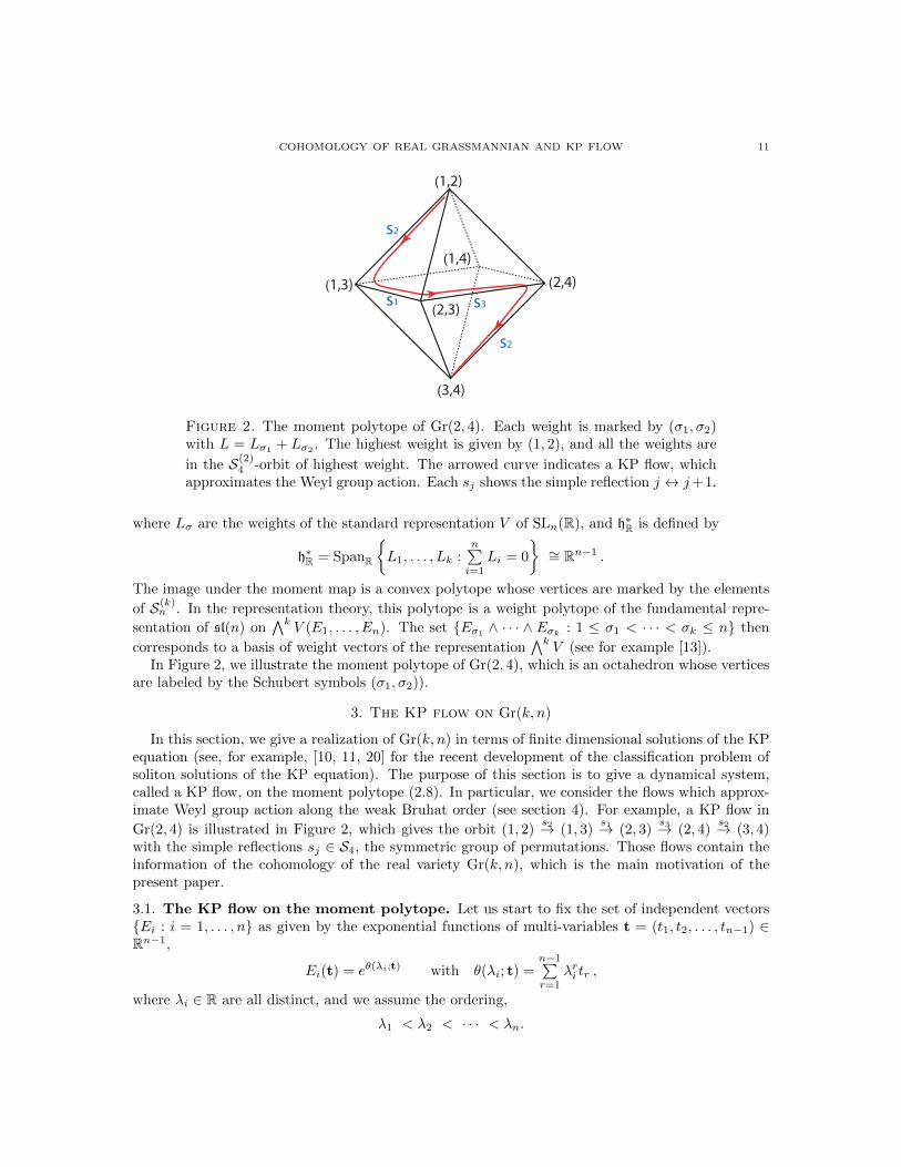
Figure 2. The moment polytope of Gr(2, 4). Each weight is marked by (σ1, σ2)with L = Lσ1 + Lσ2 . The highest weight is given by (1, 2), and all the weights are
in the S(2)4 -orbit of highest weight. The arrowed curve indicates a KP flow, which
approximates the Weyl group action. Each sj shows the simple reflection j ↔ j+1.
where Lσ are the weights of the standard representation V of SLn(R), and h∗R is defined by
h∗R = SpanR
{L1, . . . , Lk :
n∑i=1
Li = 0
}∼= Rn−1 .
The image under the moment map is a convex polytope whose vertices are marked by the elements
of S(k)n . In the representation theory, this polytope is a weight polytope of the fundamental repre-
sentation of sl(n) on∧k
V (E1, . . . , En). The set {Eσ1 ∧ · · · ∧ Eσk : 1 ≤ σ1 < · · · < σk ≤ n} then
corresponds to a basis of weight vectors of the representation∧k
V (see for example [13]).In Figure 2, we illustrate the moment polytope of Gr(2, 4), which is an octahedron whose vertices
are labeled by the Schubert symbols (σ1, σ2)).
3. The KP flow on Gr(k, n)
In this section, we give a realization of Gr(k, n) in terms of finite dimensional solutions of the KPequation (see, for example, [10, 11, 20] for the recent development of the classification problem ofsoliton solutions of the KP equation). The purpose of this section is to give a dynamical system,called a KP flow, on the moment polytope (2.8). In particular, we consider the flows which approx-imate Weyl group action along the weak Bruhat order (see section 4). For example, a KP flow in
Gr(2, 4) is illustrated in Figure 2, which gives the orbit (1, 2)s2→ (1, 3)
s1→ (2, 3)s3→ (2, 4)
s2→ (3, 4)with the simple reflections sj ∈ S4, the symmetric group of permutations. Those flows contain theinformation of the cohomology of the real variety Gr(k, n), which is the main motivation of thepresent paper.
3.1. The KP flow on the moment polytope. Let us start to fix the set of independent vectors{Ei : i = 1, . . . , n} as given by the exponential functions of multi-variables t = (t1, t2, . . . , tn−1) ∈Rn−1,
Ei(t) = eθ(λi;t) with θ(λi; t) =n−1∑r=1
λri tr ,
where λi ∈ R are all distinct, and we assume the ordering,
λ1 < λ2 < · · · < λn.

12 LUIS CASIAN AND YUJI KODAMA∗
With the set of functions {fj : j = 1, . . . , k} defined in (2.1), i.e. (f1, . . . , fk)T = A (E1, . . . , En)T
with the k×n coefficient matrix A, we define the following function, called the τ -function, given bythe Wronskian determinant of those functions,
τA(t) = Wr(f1, . . . , fk) =
∣∣∣∣∣∣∣f1 · · · fk...
. . ....
f(k−1)1 · · · f
(k−1)k
∣∣∣∣∣∣∣ ,(3.1)
Here the index A indicates the matrix A defined in (2.1). We then have:
Lemma 3.1. The τ -function can be expressed in the form,
τA(t) =∑
1≤σ1<···<σk≤nξ(σ1, . . . , σk)E(σ1, . . . , σk; t) ,
where ξ(σ1, . . . , σk) are the Plucker coordinates given by (2.4), and
E(σ1, . . . , σk; t) = Wr(Eσ1 , . . . , Eσk) =∏i<j
(λσj − λσi) exp θ(σ1, . . . , σk; t) ,
with θ(σ1, . . . , σk; t) :=k∑i=1
θ(λσi ; t).
This Lemma is a direct consequence of the Binet-Cauchy theorem (see p.9 in [14]). With theformula for f1 ∧ · · · ∧ fk in (2.3), the τA-function gives a realization of the corresponding point onGr(k, n) with the identification τA ≡ cτA for any nonzero constant c (the projectivization). Namely,
the Wronskian-map can be considered as the Plucker embedding, Wr : Gr(k, n) ↪→ RP (nk)−1. Here
one should note thatk∑i=1
λσi should be distinct for all (σ1, . . . , σk). Then one can identify the set
{E(σ1, . . . , σk; t)} as the basis {Eσ1 ∧ · · · ∧ Eσk} of ∧kRn.One can also define a map ϕA : Rn−1 → h∗R as the composite map, ϕA = µ ◦ τA, with
ϕA(t) =
∑1≤σ1<···<σk≤n
|ξ(σ1, . . . , σk)E(σ1, . . . , σk; t)|2 (Lσ1 + · · ·+ Lσk)∑1≤σ1<···<σk≤n
|ξ(σ1, . . . , σk)E(σ1, . . . , σk; t)|2.
Then if A is in the top cell, one can see that the closure of the set {ϕ(t) : t ∈ Rn−1} is a convexhull with the vertices given by the weights {Lσ1
+ · · · + Lσk : 1 ≤ σ1 < · · · < σk ≤ n}, denoted byConv(k, n), i.e.
Conv(k, n) = {ϕA(t) : t ∈ Rn−1} .This map defines a flow on the polytope, and we are interested in studying the zero set of the τAfunction which is determined by a particular choice of the coefficient matrix A.
Example 3.1. Let us consider the case Gr(2, 4) to show how one can see the polytope in Figure 2from the KP flow. Figure 3 illustrates the contour plots of the t-evolution of the solution u(x, y, t).Then as we explained in the introduction, the polytope can be seen from the dual graph of thesolution pattern as shown in the figure. Here we take the matrix A in the form,
A =
(1 1 1 1λ1 λ2 λ3 λ4
).
Note here that the 2 × 2 minors of A are all positive, i.e. ξ(i, j) = λj − λi > 0 with the orderingin λj ’s, and this implies the τ -function is positive definite and no blow-up in the KP flow. Wethen extend this example to the case with some signs in the Plucker coordinates, and show that the

COHOMOLOGY OF REAL GRASSMANNIAN AND KP FLOW 13
-75 -50 -25 0 25 50 75
-75
-50
-25
0
25
50
75 (1,4)
(1,2)
(2,3)-75 -50 -25 0 25 50 75
-75
-50
-25
0
25
50
75
(1,4)
(1,2)
(2,3)
(3,4)
-75 -50 -25 0 25 50 75
-75
-50
-25
0
25
50
75(1,4)
(3,4)
(2,3)
Figure 3. Soliton solution of the KP equation on Gr(2, 4). The figures show thecontour plot of the solution u(x, y, t) for t < 0 (left), t = 0 (middle) and t > 0(right). Each pair of numbers (i, j) indicates the dominant exponential E(i, j), i.e.the Plucker coordinates. The bounded region in the left (right) figure correspondsto E(1, 3) (E(2, 4)). The light colored graph in the figures shows the dual graphwhose vertices represent those dominant exponentials, and is the moment polytope(tetrahedron) shown in Figure 2.
flow associated with a particular choice of the signs can provide topological information of the realGrassmannians.
3.2. The KP equation and the Toda lattice. As we explained in Introduction, the function
u(x, y, t) = 2∂2
∂x2ln τA(x, y, t),
satisfies the KP equation with the identification t1 = x, t2 = y and t3 = t. The higher times, tj forj > 3, give the symmetry parameters of the KP equation, and the set of all the flows parametrizedby tj ’s forms the so-called KP hierarchy (see for example [25, 11, 20]).
In this paper, we consider a particular set of independent functions {fi : i = 1, . . . , k} such that
fi =∂i−1
∂ti−11
f =: f (i−1), with f =n∑j=1
εjEj ,
where we take εj ∈ {±}, and the set of signs (ε1, . . . , εn) is referred to as the KP sign. Note herethat the k × n coefficient matrix A is then given by
(3.2) A =
1 1 · · · 1λ1 λ2 · · · λn...
.... . .
...
λk−11 λk−1
2 · · · λk−1n
hε,
where hε is the diagonal matrix whose entries are ±1, i.e. hε := diag(ε1, . . . , εn). This matrixspecifies the blow-ups of the KP flow, and plays an important role for our study (subsection 5.1).Because of the ordering λ1 < · · · < λn, the sign of each Plucker coordinate is given by
(3.3) sign(ξ(σ1, . . . , σk)) =
k∏j=1
εσj =: ε(σ1, . . . , σk),
which will be used as the sign for the Schubert cell Xwσ = (σ1, . . . , σk) (see subsection 5.1).

14 LUIS CASIAN AND YUJI KODAMA∗
Without loss of generality, we choose the parameters λj in Ej withn∑j=1
λj = 0 (since the matrix
L can be shifted by a constant in the diagonal, i.e. L→ L+ cI with the identity matrix I does notchange the equation). Then the set of τ -functions,
(3.4) τk := Wr(f, f ′, . . . , f (k−1)), k = 1, 2, . . . , n.
gives the solution of the Toda lattice equation for SLn(R), which is defined with the n×n tri-diagonalmatrix L,
L =
b1 1 0 · · · 0a1 b2 1 · · · 0...
. . .. . .
. . ....
0 · · · · · · bn−1 10 · · · · · · an−1 bn
The Toda lattice equation is then expressed by the matrix equation (i.e. the Lax equation),
dL
dt= [L,L−],
where L− represents the (strictly) lower triagular part of the matrix L. The solution is then givenby
(3.5) aj =τj+1τj−1
τ2j
bj =d
dtln
τjτj−1
,
with τ0 = 1. The Toda lattice equation has several commuting flows, and the set of those flowsforms the Toda lattice hierarchy which can be defined as
∂L
∂tj= [L,Lj−] with Lj− := (Lj)−, j = 1, 2, . . . , n− 1.
Note that each τk then gives a solution of the KP equation on Gr(k, n) with the identificationst1 = x, t2 = y and t3 = t. The solution of the Toda lattice hierarchy is given by the set (τ1, . . . , τn−1)
(note τn is just a constant, sincen∑j=1
λj = 0). Since each τk can be considered as a point of Gr(k, n),
the solution of the Toda lattice equation defines a point of the flag manifold B := SLn(R)/B withthe Borel subgroup B. This is just a consequence of the diagonal embedding, denoted by ι, of Binto the product of the Grassmannians, i.e.
ι : B ↪→ Gr(1, n)×Gr(2, n)× · · · ×Gr(n− 1, n).
We then define a map ϕ : Rn−1 → h∗R as the composite map ϕ = µ ◦ ι,
ϕ(t) =n−1∑k=1
µ(τk(t)),
where µ : Gr(k, n) → h∗R is the moment map defined in (2.8). The moment polytope for the Todalattice hierarchy is the permutohedron of the symmetric group Sn, whose vertices are labeled by theelements of Sn. In [8], we used this fact, and described the cohomology of the real flag variety interms of the Toda flow and its blow-ups. We basically follow the arguments given in that paper.However we have found several new structures for the case of Gr(k, n), not just by a projectionπ : B → Gr(k, n), and in fact, we found the explicit form of the Poincare polynomials for Gr(k, n).Figure 4 illustrates the moment polytope (permutohedron) for SL4(R) Toda lattice hierarchy. Thefigure shows the incidence graph of the real flag variety B = SL4(R)/B as shown in [8].
Each τ -function gives the zero divisor on the polytope which corresponds to the singular solutionof the Toda lattice hierarchy. Although one can recover the incidence graph of Gr(k, 4) from the

COHOMOLOGY OF REAL GRASSMANNIAN AND KP FLOW 15
e
[321][2321]
[1321]
[21321]
[12321]
w =[121321]
[1]
[2]
[3]
o
Figure 4. The moment polytope of SL4(R) Toda lattice hierarchy with the signsεj := sign(aj) = − for all j = 1, 2, 3. Each vertex is marked by the element of thesymmetric group S4, which is denoted by [i1i2 . . . ij ] = si1si2 · · · sij The three sub-graphs indicated by the thick edges with different colors correspond to the incidencegraphs of Gr(k, 4). Namely, the edges connecting with the vertices {e, [1], [21], [321]}corresponds to Gr(1, 4), the edges with {e, [2], [12], [32], [312], [2312]} corresponds toGr(2, 4), and those with {e, [3], [23], [123]} for Gr(3, 4). The zero sets of the τ -functions are shown by the curves crossing the edges (see [8]). For example, thedotted curve shows τ1 = 0, the light color curve shows τ2 = 0, and the dark oneshows τ3 = 0.
Figure as the subgraph of this flag picture, in this paper we give an alternative construction basedon the KP low which leads to explicit cohomology calculations. We do use the flag picture based onthe Toda flow to prove our main theorem 1.1. Below we explain the links, similarities and differencesbetween the Toda and the KP approaches with an example.
3.3. Remark on the Toda lattice description. Here using the SL4(R) Toda lattice, we give abrief overview of the results in [8] on the incidence graph of the real flag manifold B = SL4(R)/B.The cohomology of B then arises from the Toda lattice with the Toda signs εj = sign(aj) (seeDefinition 6.2 below) attached to the vertex e given by εj = − for all j = 1, 2, 3. Since the solution(aj , bj) of the Toda lattice is given in the form (3.5), the τ1-function has the form,
τ1 = E1 − E2 + E3 − E4,
that is, we have the KP signs (ε1, . . . , ε4) = (+,−,+,−) (the solution corresponding to this choiceof the signs has the maximum number of blow-ups from t → −∞ to t → ∞, see [21]). Note thatfrom (3.5), the Toda signs are defined with the εj ’s in the τ1-function in the form,
εj := sign(aj) = ε−1j εj+1.
This corresponds to the relation between the roots α and the fundamental weights ω, i.e. with thecharacter χ of the group, they are defined by ε = −χα(h) and ε = −χω(h) for h ∈ H, the Cartansubgroup [5] (see also subsection 6.5). Then the sign change along the edge w → siw is given by(Proposition 5.1 in [8], see also Proposition 6.1)
ε′j = εj ε−Ci,ji ,

16 LUIS CASIAN AND YUJI KODAMA∗
where Ci,j is the Cartan matrix for SL4(R). The co-boundaries involving two vertices w and siware zero when one crosses a blow-up (singularity), that is, the edge crosses τi = 0, (i.e. εj ε
′j = −).
Then the incidence graph of Gr(k, 4) is obtained as a subgraph of the incidence graph for the flagmanifold. If we consider Gr(1, 4) then the incidence graph is the subgraph containing the vertices{e, s1, s2s1, s3s2s1}. In Figure 4, this is the subgraph connecting with the vertices {e, [1], [21], [321]}which crosses curves of the form τi = 0 twice. That is, along s1 one crosses τ1 = 0, then alongthe edge from [1] to [21] none of the τk = 0 are crossed, hence there is a non-zero co-boundary.Finally along the edge connecting [21] and [321] , τ3 becomes zero, i.e. the co-boundary is zero. Thisgives the incidence graph giving the cohomology of Gr(1, 4), that is, we have the graph, e → s1 ⇒s2s1 → s3s2s1. In general, the incidence graph of the partial flag G/P appears as a subgraph of theincidence graph of the flag G/B (see [9] and Remark 6.1 below ).
In this paper, we consider the cohomology of Gr(k, n) directly from the KP flow, that is, weconstruct the incidence graph based on a single τ -function, i.e. τk. One should then note that forexample, the incidence graph of Gr(1, 4) from the KP flow is obtained by the choice of the τ -functionin (1.2), i.e. we have (ε1, . . . , ε4) = (+,−,−,+) as we discussed above. Notice that the correspondingToda sign is (ε1, ε2, ε3) = (−,+,−), which is not the same as the Toda signs used for the flag pictureof Figure 4. The Toda sign (−,+,−) would give an incidence graph for cohomology with twistedcoefficients of the real flag manifold and this is not described by Figure 4. (See Figure 4 in [6] forthe moment polytopes with different signs (ε1, ε2, ε3).)
In order to get the incidence graph of Gr(1, 4) in terms of the KP flow, that is related to theToda flow with sign (−,+,−) and taking into account only the flow as it crosses τ1 = 0, we thenneed to consider the quotient S4/〈s2, s3〉 corresponding to the natural projection, π : G/B → G/Pwith the maximum parabolic P . Namely we are now in Gr(1, 4) viewed as SL4(R)/P and in thisquotient τ1 = 0 is crossed by that edge of the tetrahedron, and so we recover the incidence graph ofGr(1, 4). This is illustrated in Figure 1. Also note that the projection π : G/B → Gr(2, 4) gives theoctahedron illustrated in Figures 2 and 3.
It turns out that there are exactly two distinguished Toda signs (and two corresponding distin-guished KP signs) which need to be used for the cohomology of all the Gr(k, n) to be expressedin terms of the KP flow. For example, in the case Gr(k, 4), these are (−,+,−) for k = 1, 3 and(+,−,+) for k = 2. Note once more, that the Toda sign (ε1, ε2, ε3) giving the incidence graph in[8] (cohomology with constant coefficients), or in Figure 4, is not one of these two, but rather it isassociated to (−,−,−).
A summary of the strategy in the proof of our main theorem given in section 6 can be expressedas follows. The point is to check that the incidence graph of Gr(k, n), viewed as a subgraph of theincidence graph of the real flag manifold, derived from the Toda lattice and corresponding to theToda signs εi = − for all i, agrees with a graph defined in terms of the KP flow and one of the twodistinguished KP signs.
4. The set S(k)n and the graph G(k)
n
In this section, we describe the algebraic structure of the Grassmannian Gr(k, n). The set ofSchubert cells {(σ1, . . . , σk) : 1 ≤ σ1 < · · · < σk ≤ n} for Gr(k, n) forms a partially orderedset (poset) with the Bruhat order defined as follows: Let si ∈ Sn be an adjacent transpositionsi : i → i + 1 for i = 1, . . . , n − 1 for the symmetric group Sn. Then there exists sσi-action on thecell (σ1, . . . , σk), if σi + 1 < σi+1 for some i or σk < n. The action gives
sσi : (σ1, . . . , σi, . . . , σk) −→ (σ1, . . . , σi−1, σi + 1, σi+1, . . . , σk) .
Then the arrow given by the action determines the weak Bruhat order between those cells. Withaction defined this way, each cell can be uniquely parametrized by a representative of minimal length

COHOMOLOGY OF REAL GRASSMANNIAN AND KP FLOW 17
in the quotient Sn/Pk (see [2]), that is,
S(k)n := {the reduced words of mod(Pk) ending in sk}.
Here Pk is a Weyl subgroup of Sn corresponding to the maximal parabolic subgroup, and is generatedby {s1, . . . , sk−1, sk+1, . . . , sn−1}, denoted as
Pk = 〈s1, . . . , sk, . . . , sn−1〉 ∼= Sk × Sn−k.
Note here that Pn = Sn and S(n)n = {e}. In this sense, we identify an element wσ ∈ S(k)
n with the
Schubert cell σ = (σ1, . . . , σk). This leads to the Schubert decomposition in terms of S(k)n , that is,
we have
Gr(k, n) =⊔
wσ∈S(k)n
Xwσ , with Xwσ = (σ1, . . . , σk).
We also write Xwσ simply as wσ, that is, wσ = (σ1, . . . , σk). With the set S(k)n , one should also note
|Gr(k, n,Fq)| =∑
w∈S(k)n
ql(w) ,
where l(w) is the length of w.The set of Schubert cells with si-actions forms a graph consisting of the vertices given by the cells
and the edges given by the weak Bruhat order. We denote this graph by G(k)n , and call it the weak
Bruhat graph of Gr(k, n). Let us give few examples of G(k)n .
Example 4.1. We consider the cases with n = 4 and k = 1, 2, 3:
(1) Gr(1, 4) ∼= RP 3 : The graph G(1)4 is given by
(1)s1−→ (2)
s2−→ (3)s3−→ (4) .
Each cell (k) can be parametrized by an element in S(1)4 , the set of minimal length repre-
sentative in the quotient S4/〈s2, s3〉, that is, (1) = e, (2) = s1, (3) = s2s1, (4) = s3s2s1.
(2) Gr(2, 4) : The graph G(2)4 is given by
(1, 2)s2−→ (1, 3)
s3−→ (1, 4)ys1 ys1(2, 3)
s3−→ (2, 4)ys2(3, 4)
.
Each cell (i, j) is parametrized by a unique element of S(2)4 , i.e. (1, 2) = e, (1, 3) = s2, (2, 3) =
s1s2, (1, 4) = s3s2, (2, 4) = s1s3s2, (3, 4) = s2s1s3s2.
(3) Gr(3, 4) ∼= RP 3: The graph G(3)4 is given by
(1, 2, 3)s3−→ (1, 2, 4)
s2−→ (1, 3, 4)s1−→ (2, 3, 4) .
The parametrization of each cell (i, j, k) is given by (1, 2, 3) = e, (1, 2, 4) = s3, (1, 3, 4) =
s2s3, (2, 3, 4) = s1s2s3. Those are the elements of S(3)4 .

18 LUIS CASIAN AND YUJI KODAMA∗
4.1. The decomposition of S(k)n . Here we consider a decomposition of the set S(k)
n into the set
{S(k−1)j−1 : j = k, k+1, . . . , n}. This decomposition is based on the following relation for the binomial
coefficients, (n
k
)=
(k − 1
k − 1
)+
(k
k − 1
)+ · · ·+
(n− 1
k − 1
)=
n∑j=k
(j − 1
k − 1
).
which is a direct consequence of the Pascal rule,(nk
)=(n−1k
)+(n−1k−1
). Namely we have:
Proposition 4.1. The set S(k)n has a decomposition,
S(k)n = S(k−1)
k−1 ∪n−1⋃j=k
S(k−1)j sj · · · sk ,
where note S(k−1)k−1 = {e}.
To prove Proposition 4.1, we first state the following Lemma which is similar to the Pascal rule,
Lemma 4.2. There is a decomposition,
S(k)n = S(k)
n−1 ∪ S(k−1)n−1 sn−1sn−2 · · · sk .
Proof. This corresponds to the decomposition of weight vectors,
k∧V (E1, . . . , En) =
k∧V (E1, . . . , En−1)⊕
[k−1∧
V (E1, . . . , En−1) ∧ En
].
It is then obvious that the weight vectors in the fast part are given by the orbit of S(k)n−1 of the
highest weight vector E1 ∧ · · · ∧ Ek.Now note that the element w = sn−1 · · · sk maps the highest weight vector E1 ∧ · · · ∧ Ek to
E1∧· · ·∧Ek−1∧En. Then the weight vectors in ∧k−1V (E1, . . . , En−1) can be obtained by the orbit
of S(k−1)n−1 of the highest weight vector E1 ∧ · · · ∧ Ek−1.
Remark 4.1. The decomposition in Proposition 4.1 corresponds to the following decomposition,
k∧V (E1, . . . , En) =
n⊕j=k
[k−1∧
V (E1, . . . , Ej−1) ∧ Ej
].
Example 4.2. The set S(2)4 can be written as S(1)
1 ∪ S(1)2 s2 ∪ S(1)
3 s3s2: First we write the sets S(k)m
which are involved,
(4.1) S(1)1 = {e}, S(1)
2 = {e, s1}, S(1)3 = {e, s1, s2s1}.
Hence we have
(4.2) S(1)1 ={e}, S(1)
2 s2 ={s2, s1s2}, S(1)3 s3s2 ={s3s2, s1s3s2, s2s1s3s2}.
As in Remark 4.1 we have a decomposition
2∧V (E1, E2, E3) =
[1∧V (E1) ∧ E2
]⊕
[1∧V (E1, E2) ∧ E3
]⊕
[1∧V (E1, E2, E3) ∧ E4
].
For example,∧V (E1, E2, E3) ∧ E4 corresponds to S(1)
3 s3s2. This is given explicitly by associatingE1 ∧E4, E2 ∧E4, E3 ∧E4 to the elements s3s2, s1s3s2, s2s1s3s2 respectively (see also Example 4.5below).

COHOMOLOGY OF REAL GRASSMANNIAN AND KP FLOW 19
The decomposition of S(k)n provides an arrangement of the Schubert decomposition of Gr(k, n):
(4.3) Gr(k, n) =
n⊔j=k
⊔1≤σ1<···<σk−1≤j−1
X(σ1, . . . , σk−1, j)
.
Each Schubert cell X(σ1, . . . , σk−1, j) can be labeled by an element of S(k−1)j sj · · · sk. For each set
S(k−1)j , we can define the Bruhat graph G(k−1)
j . We then have a decomposition of the graph G(k)n ,
G(k)n =
[G(k−1)k−1
sk−→ G(k−1)k
sk+1−→ · · · · · · sn−1−→ G(k−1)n−1
].
Here the sj-action provides the edges connecting the vertices in G(k−1)j−1 with the corresponding
vertices in G(k−1)j , i.e.
G(k−1)j−1 3 (σ1, . . . , σk−1, j )
sj−→ (σ1, . . . , σk−1, j+1 ) ∈ G(k−1)j ,
for all 1 ≤ σ1 < · · · < σk−1 ≤ j − 1, and each index in the box is fixed.
Example 4.3. Consider the case of Gr(3, 5). The graph G(3)5 is given by
(1, 2, 3 )s3−→ (1, 2, 4 )
s4−→ (1, 2, 5 )↓ ↓
(1, 3, 4 )s4−→ (1, 3, 5 ) −→ (1, 4, 5 )
↓ ↓ ↓(2, 3, 4 )
s4−→ (2, 3, 5 ) −→ (2, 4, 5 )↓
(3, 4, 5 )
which has the structure of a sequence of smaller graphs, i.e. the decomposition of the graph G(3)5 ,
G(3)5 =
[G(2)
2s3−→ G(2)
3s4−→ G(2)
4
].
4.2. The decomposition of Gr(k, n). We now describe a decomposition of Gr(k, n) based on thearrangement (4.3). Let us first define Y (j) for j = k, k+ 1, . . . , n as the unions of the Schubert cellsin (4.3),
Y (j) :=⊔
1≤σ1<···<σk−1≤j−1
X(σ1, . . . , σk−1, j) .
Then we explain that each Y (j) is a manifold with the structure of a vector bundle. To do this, letus fix vector spaces {V0(j) : j = k − 1, k, . . . , n} satisfying
V0(k − 1) ⊂ V0(k) ⊂ · · · ⊂ V0(n− 1) ⊂ V0(n) = Rn ,with dim(V0(j)) = j. Then Y (j) can be described by
Y (j) = {[V ] : V ⊂ V0(j), dim(V ∩ V0(j − 1)) = k − 1} for j = k, k + 1, . . . , n.
Now one can see that Y (j) is a manifold which has the structure of a vector bundle V(j) withfibers of dimension j − k over the Grassmanian Gr(k − 1, j − 1). We have well defined projectionsπj : Y (j) → Gr(k − 1, j − 1) which are given by πj([V ]) = [V ∩ V0(j − 1)]. This is becauseV ∩V0(j− 1) ⊂ V0(j− 1) is a vector space of dimension k− 1 inside a fixed vector space which lookslike Rj−1. The fibers of this projection can be computed using explicit coordinates (see below).These vector bundles determine the determinant line-bundles over Gr(k − 1, j − 1),
(4.4)
j−k∧V(j) = E(j).

20 LUIS CASIAN AND YUJI KODAMA∗
Remark 4.2. We have the following:
(i) The space Y (j) is a union of cells corresponding to S(k−1)j−1 sj−1 · · · sk ↔ G(k−1)
j−1
(ii) Each element in S(k−1)j−1 labels a corresponding cell in Gr(k − 1, j − 1).
(iii) The cell of lowest dimension in Y (j) corresponds to sj−1 · · · sk.• The union of all these cells {sj−1 · · · sk : j = k+1, · · ·n−1} correspond to the incidence
graph of RPn−k ∼= Gr(1, n− k + 1).• These cells of RPn−k are the ones associated to the Schubert symbols
(1, 2, . . . , k − 1, j), for j = k, . . . , n .
• These are also the elements sj · · · sk in the statement of Proposition 4.1 and in Example4.2 these are the cells labeled as e, s2, s3s2.
(iv) The fibers of the vector bundles V(j) with total space Y (j) and base Gr(k − 1, j − 1)correspond to the cells of this RPn−k.
In the following examples, we describe explicitly the cells involved in each piece of this decompo-
sition and the correspondence between a cell decomposition of Y (j) and∧k−1
V (E1, . . . , Ej−1)∧Ej .The basis element Eσ1
∧ · · · ∧ Eσk−1∧ Ej label a cell with pivots at the positions (σ1, . . . , σk−1, j).
Example 4.4. Explicit decomposition in the case of Gr(2, 3) ∼= RP 2. Let V0(2) ⊂ R3 consist ofvectors of the form (x1, x2, 0). We let V denote a two dimensional vector space in R3 and [V ] acorresponding point in Gr(2, 3). We than have
Y (2) ={[V0(2)]} =
{(1 0 00 1 0
)},
Y (3) ={[V ] : V ⊂ R3, dim(V ∩ V0(2)) = 1}
=
{(1 0 00 ∗ 1
)}t{(∗ 1 0∗ 0 1
)}.
Looking at the position of pivots Y (2) should be thought as corresponding to∧1
V (E1) ∧ E2 and
Y (3) to the summand∧1
V (E1, E2) ∧ E3 in a decomposition of∧2
V (E1, E2, E3).If we think of Gr(2, 3) ∼= RP 2 given as a sphere where antipodal points are identified, then this
decomposition has a simple description. First Y (2) can be identified with the north and south poles.If we delete this pair of antipodal points we are left with a Mobius band corresponding to Y (3).This is a non-trivial line bundle over the equator and in matrix notation, π3 projects a matrix to itsfirst row so that π3(Y (3)) = {(1 0 0)} t {(∗ 1 0)} ∼= RP 1). The one dimensional fibers are given bythe second row in a matrix i.e. (0 ∗ 1) and (∗ 0 1) over {(1 0 0)} and {(∗ 1 0)}, respectively.
The RP 1 in item (iii) of Remark 4.2 is a meridian. Note that the direction along meridianscorresponds to the fibers of the fiber bundle over the equator giving the Mobius band.
Example 4.5. Explicit decomposition in the case of Gr(2, 4). We once more emphasize the con-nection with a decomposition:
(4.5)
2∧V (E1, E2, E3, E4) =
[1∧V (E1) ∧ E2
]⊕
[1∧V (E1, E2) ∧ E3
]⊕
[1∧V (E1, E2, E3) ∧ E4
].

COHOMOLOGY OF REAL GRASSMANNIAN AND KP FLOW 21
Let V0(2) ⊂ V0(3) ⊂ R4 be two subspaces of dimensions 2 and 3 respectively. We let V denote atwo dimensional vector space in R4 and [V ] a corresponding point in Gr(2, 4). Set:
Y (2) ={[V0(2)]} =
{(1 0 0 00 1 0 0
)},
Y (3) ={[V ] : V ⊂ V0(3), dim(V ∩ V0(2)) = 1}
=
{(1 0 0 00 ∗ 1 0
)}t{(∗ 1 0 0∗ 0 1 0
)},
Y (4) ={[V ] : V ⊂ R4, dim(V ∩ V0(3)) = 1}
=
{(1 0 0 00 ∗ ∗ 1
)}t{(∗ 1 0 0∗ 0 ∗ 1
)}t{(∗ ∗ 1 0∗ ∗ 0 1
)}.
We have Y (2) = Gr(2, 2) ∼= Gr(1, 1), Y (3) is a non-trivial line bundle over Gr(1, 2), and Y (4) is anon-trivial R2 bundle over Gr(1, 3). The projections of these bundles are π3 : Y (3)→ Gr(1, 2) withπ3([V ]) = [V ∩V0(2)], and π4 : Y (4)→ Gr(1, 3) with π4([V ]) = [V ∩V0(3)]. More explicitly, we have
π3(Y (3)) ={(1 0 0 0)} t {(∗ 1 0 0)} = Gr(1, 2),
π4(Y (4)) ={(1 0 0 0)} t {(∗ 1 0 0)} t {(∗ ∗ 1 0)} = Gr(1, 3).
The fiber over {(1 0 0 0)} in Y (3) is (0 ∗ 1 0), and the fiber over {(∗ 1 0 0)} is (∗ 0 1 0). Thisbecomes a non-trivial line bundle over the circle Gr(1, 2). The case of Y (4) is described similarlyand results in a non-trivial vector bundle with fiber of dimension 2. The fiber over {(1 0 0 0)} is{(0 ∗ ∗ 1)}, the fiber over {(∗ 1 0 0)} is {(∗ 0 ∗ 1)}, and the fiber over {(∗ ∗ 1 0)} is {(∗ ∗ 0 1)}.The fiber of the vector bundle over Gr(1, 3) is two dimensional because of the two parameters.
5. The graph G(k, n)
Here we define what will be shown to be the incidence graph for the cohomology of Gr(k, n)relative to Schubert cells. We first consider the case of Gr(1, n) ∼= RPn−1, and then introduce signedSchubert cells to construct what will become the incidence graph. The goal of this section is toshow that this graph defined for Gr(k, n) can be obtained from the results of Gr(1, n) and its dualGr(n− 1, n).
Let us recall that Gr(1, n) ∼= RPn−1 has the Schubert decomposition,
Gr(1, n) =⊔
1≤σ1≤n
X(σ1) ,
where X(σ1) is the Schubert cell given by X(i) = {(x1, . . . , xi−1, 1, 0, . . . , 0) : xj ∈ R} ∼= Ri−1. Thenthe cochain complex for Gr(1, n) is expressed by
(5.1) Z[〈(1)〉] δ0−→ Z[〈(2)〉] δ1=⇒ · · · · · · δ2m−2−→ Z[〈(2m)〉] δ2m−1=⇒ Z[〈(2m+ 1)〉] δ2m−→ · · · .
with 〈(i)〉 = X(i) and the coboundary operator δi : Z[〈(i+ 1)〉]→ Z[〈(i+ 2)〉]. Here the single arrow→ indicates 0 incidence number and the double arrow indicates nonzero incidence number which iseither 2 or −2 [19], i.e.
δi−1〈(i)〉 =
{0 if i = odd±2 〈(i+ 1)〉 if i = even
Then we recover the well-known formulas of the integral cohomology of Gr(1, n) ∼= RPn−1 as follows:

22 LUIS CASIAN AND YUJI KODAMA∗
(a) For n = 2m+ 1, the last arrow in (5.1) is the double arrow, and we have
Hk(RP 2m;Z) =
Z if k = 00 if k = odd ≤ 2m− 1Z2 if k = even ≤ 2m
The Poincare polynomial for Gr(1, 2m+ 1) is then just P(1,2m+1)(t) = 1.(b) For n = 2m+ 2, the last arrow is the single one, and
Hk(RP 2m+1;Z) =
Z if k = 0 and if k = 2m+ 10 if k = odd 6= 2m+ 1Z2 if k = even ≤ 2m
The Poincare polynomial for this case is P(1,2m+2)(t) = 1 + t2m+1.
5.1. The signed Schubert cells. In order to represent the incidence graph in terms of the Schubertcells, we introduce the signed Schubert cells (see also subsection 3.1). Let us first define the signedvectors ej := εjEj for j = 1, . . . , n where Ej ∈ Rn is the j-th standard basis vector, and εj ∈ {±}.Then the k-wedge product eσ1
∧ · · · ∧ eσk has the sign ε(σ1, . . . , σk) =∏kj=1 εσj (see (3.3)), i.e.
eσ1∧ . . . ∧ eσk = ε(σ1, . . . , σk)Eσ1
∧ . . . ∧ Eσk .We then define a (induced) sign of the Schubert cell (σ1, . . . , σk) as the sign of the wedge producteσ1 ∧ · · · ∧ eσk , i.e. ε(σ1, . . . , σk). Thus we identify the signed cell (σ1, . . . , σk) as eσ1 ∧ · · · ∧ eσk .
Remark 5.1. With the signed bases {ej : j = 1, . . . , n}, the τ -function in (3.4) can be written in the
following form with f =k∑j=1
εjEj ,
τk = Wr(f, f ′, . . . , f (k−1))
=∑
1≤σ1<···<σk≤n|ξ(σ1, . . . , σk)|ε(σ1, . . . , σk)E(σ1, . . . , σk)
where |ξ(σ1, . . . , σk)| is the k × k minor of the Vandermonde matrix in A.
We now define a graph G(k, n), which depends on the choice of signed vectors ei and which isobtained from the weak Bruhat graph whose edges indicate that the cells connected by the edge havethe same sign. Suppose that we have sσi-action on the cell (σ1, . . . , σk), i.e. σi+1 < σi+1. Then if thecells connected by the action have the same sign, i.e. ε(σ1, . . . , σi, · · · , σk) ε(σ1, . . . , σi+ 1, . . . , σk) =+, we put the double edge for the Bruhat order, i.e.
sσi : (σ1, . . . , σi, . . . , σk) =⇒ (σ1, . . . , σi + 1, . . . , σk) .
Otherwise (i.e. sign change), we keep the single edge of the Bruhat order. Thus this new graph isobtained from the Bruhat graph by changing some of the edges to the double ones. The single edgescorrespond to the cells which have the different signs, i.e. ε(σ)ε(σ′) = − for the Bruhat ordered cellswith σ = (σ1, . . . , σk) and σ′ = (σ′1, . . . , σ
′k).
We also impose the signs for particular cells (σ1, . . . , σk) as follows:
(a) Assume ε1 = +.
(b) Assign ε(1, . . . , k − 1, k + j) = (−)bj+12 c for j = 0, 1, . . . , n− k.
(c) Assign ε(1, . . . , k − j, k − j + 2, . . . , k + 1) = (−)bj+12 c for j = 1, 2, . . . , k − 1.
The item (b) implies that we have the same sign pattern for RPn−k = Gr(1, n−k+1). The item (c)then corresponds to the pattern of RP k = Gr(k, k + 1). Those cells appear in the upper horizontalline and the left vertical side of the Bruhat graph. Then one can determine uniquely the signs(ε1, . . . , εn) for a given pair of the numbers (k, n).

COHOMOLOGY OF REAL GRASSMANNIAN AND KP FLOW 23
Proposition 5.1. Following the sign assignment given above for Gr(k, n), the signs εj are given by{ε2j+1 = (−)j for j = 0, 1, . . . , bn−1
2 c,ε2j+2 = (−)k+j for j = 0, 1, . . . , bn−2
2 c.
Proof. First we note that the sign choice in (b) leads to the condition,
εk+j−1εk+j = (−)j for j = 1, 2, . . . , n− k.
Also from the choice (c), we have
εk−j+1εk−j+2 = (−)j for j = 1, 2, . . . , k.
Combining those, we have
εjεj+1 = (−)k+j+1 for j = 1, 2, . . . , n− 1,
With the condition (a), i.e. ε1 = +, we obtain the desired formulae.This proposition implies that for Gr(k, n), if k is odd, we choose the signs,
(5.2) (ε1, ε2, ε3, ε4, . . . , εn) = (+,−,−,+, · · · , (−)bn2 c),
and if k is even, we choose
(5.3) (ε1, ε2, ε3, ε4, . . . , εn) = (+,+,−,−, . . . , (−)bn−12 c).
It will be useful to describe those sets of signs using the diagonal matrix hε defined in (3.2). Namelywe define h(−) and h(+) as the n× n diagonal matrices hε corresponding to the sets of signs (5.2)and (5.3), respectively, i.e.
h(−) :=diag(
+,−,−,+, . . . , (−)bn2 c),
h(+) :=diag(
+,+,−,−, . . . , (−)bn−12 c).
These act on V (E1, · · · , En). These matrices then belong to the group SL(n,R)± and also act on∧kV (E1, · · · , En). This gives each Ej1 ∧ · · · ∧Ejk (i.e. each cell) a sign, namely the corresponding
eigenvalue,
h(±) Eσ1 ∧ Eσ2 ∧ · · · ∧ Eσk = ε(σ1, σ2, . . . , σk) Eσ1 ∧ Eσ2 ∧ · · · ∧ Eσk .
The graph that has been constructed has vertices (σ1, · · · , σk)←→ Eσ1∧ · · · ∧ Eσk . For k odd, we
consider the action h(−), and for k even, the action of h(+). An edge⇒ exists between two verticesrelated by a simple reflection whenever the signs (eigenvalues of h(±) ) agree for the two elements
in∧k
V (E1, · · · , En).
Remark 5.2. In the identification of the Schubert cell (σ1, . . . , σk) with the wedge vector Eσ1 ∧ · · · ∧Eσk , the action between two cells in the weak Bruhat order can be considered as the KP flow throughthe corresponding two dominant exponentials. Then changing the sign ε(σ1, . . . , σk) is equivalent tohaving a zero in the τ -function. That is, the KP flow has a singularity.
Notation 5.1. With the diagonal action of h(±), we can refer to this graph denoted by G(k, n) as
the graph associated to the action of h(±) on∧k
V (E1, · · · , En). It will be shown that this graphis an incidence graph computing cohomology of Gr(k, n) relative to Schubert cells.
We now state the main theorem.
Theorem 5.2. The graph G(k, n) of h(±) acting on∧k
V (E1, · · · , En) agrees with the incidencegraph of Gr(k, n).

24 LUIS CASIAN AND YUJI KODAMA∗
We prove the Theorem in the section 6. Before closing this section, we give some lower dimensionalexamples.
Example 5.1. Let us first consider Gr(2, 4): With the signs (ε1, . . . , ε4) = (+,+,−,−), we obtain
(1, 2) → (1, 3) ⇒ (1, 4)⇓ ⇓
(2, 3) ⇒ (2, 4)↓
(3, 4)
This is the incidence graph of Gr(2, 4) and the nonzero incidence numbers are ±2. This graph is, ofcourse, a subgraph of the incidence graph for the real flag manifold shown in Figure 4. The integralcohomology H∗(Gr(2, 4),Z) is then given by
H0(Gr(2, 4),Z) = Z, H3(Gr(2, 4),Z) = Z2,H1(Gr(2, 4),Z) = 0, H4(Gr(2, 4),Z) = Z,H2(Gr(2, 4),Z) = Z2,
It is interesting to note that the Betti numbers β0 = 1 and β4 = 1 are coming from the cells with(1, 2) and (3, 4), respectively. The corresponding Young diagrams for those cells are given by
(1, 2) = ∅, (3, 4) = .
Here the Young diagram associated to the cell (σ1, . . . , σk) is defined by (ν1, . . . , νk) with νj =σk−j+1 − (k − j + 1) (note νj ≥ νj+1 as the usual definition of the Young diagram, and each νjexpresses the number of boxes in the row of the diagram).
Remark 5.3. Note that the top row of the graph corresponds to the elements
E1 ∧ E2 → E1 ∧ E3 ⇒ E1 ∧ E4.
These terms E2, E3, E4 already appeared in the decomposition (4.5) in Example 4.5 indicating theposition of a pivot. They now corresponds to a portion of the graph of RP 3 with twisted coefficients,
which agrees with the graph of RP 2 with constant coefficients, and is indicated with︷︸︸︷· · · ,
E1 ⇒︷ ︸︸ ︷E2 → E3 ⇒ E4 .
In general the top row of the graph is one of the following depending on whether k is odd or even:
(a) If k is odd, we have h(−) action, and
E1 ∧ · · · ∧ Ek−1 ∧ Ek ⇒ E1 ∧ · · · ∧ Ek−1 ∧ Ek+1 → E1 ∧ · · · ∧ Ek−1 ∧ Ek+2 ⇒ · · ·
(b) If k is even, we have h(+) action, and
E1 ∧ · · · ∧ Ek−1 ∧ Ek → E1 ∧ · · · ∧ Ek−1 ∧ Ek+1 ⇒ E1 ∧ · · · ∧ Ek−1 ∧ Ek+2 → · · ·
We summarize the argument above as the following Lemma.
Lemma 5.3. We have the following.
(i) The top row of the graph G(k, n) associated to the action of h(−) on∧k
V (E1, · · ·En) is theincidence graph of RPn−k with trivial coefficients if k is odd and with twisted coefficients ifk is even.
(ii) The top row of the graph G(k, n) associated to the action of h(+) on∧k
V (E1, · · ·En) is theincidence graph of RPn−k with twisted coefficients if k is even and with trivial coefficientsif k is odd.

COHOMOLOGY OF REAL GRASSMANNIAN AND KP FLOW 25
Example 5.2. We now consider Gr(3, 6): The action is then given by h(−) = diag(+,−,−,+,+,−),and the graph is given by
(1, 2, 3)0 (1, 2, 4)1 ⇒ (1, 2, 5)2 (1, 2, 6)3
⇓ ⇓ ⇓(1, 3, 4)2 ⇒ (1, 3, 5)3 (1, 4, 5)4 (1, 3, 6)4 (1, 4, 6)5 ⇒ (1, 5, 6)6
(2, 3, 4)3 ⇒ (2, 3, 5)4 (2, 4, 5)5 (2, 3, 6)5 (2, 4, 6)6 ⇒ (2, 5, 6)7
⇓ ⇓ ⇓(3, 4, 5)6 (3, 4, 6)7 ⇒ (3, 5, 6)8
(4, 5, 6)9
Here the single arrows (corresponding to the zero incidence numbers) are all eliminated. The suffix
in each cell shows the dimension of the cell, that is, the dimension d is given by d =3∑j=1
(σj − j) for
each cell of (σ1, σ2, σ3). The cohomology is then given by
H0(Gr(3, 6),Z) = Z, H5(Gr(3, 6),Z) = Z,H1(Gr(3, 6),Z) = 0, H6(Gr(3, 6),Z) = Z2 ⊕ Z2,
H2(Gr(3, 6),Z) = Z2, H7(Gr(3, 6),Z) = Z2,
H3(Gr(3, 6),Z) = Z2, H8(Gr(3, 6),Z) = Z2,
H4(Gr(3, 6),Z) = Z⊕ Z2 ⊕ Z2, H9(Gr(3, 6),Z) = Z.
Note here that the Betti numbers β0 = 1, β4 = 1, β5 = 1 and β9 = 1 are coming from the Schubertcycles with (1, 2, 3), (1, 4, 5), (2, 3, 6) and (4, 5, 9), and the Young diagrams of those cycles are givenby
(1, 2, 3) = ∅, (1, 4, 5) = , (2, 3, 6) = , (4, 5, 6) = .
The Young diagram for (4, 5, 6) may be considered to be a combination of (1, 4, 5) and (2, 3, 6). Thispattern is common for the case of Gr(k, n) with k =odd and n =even (see Section 8)
6. Proof of the main Theorem for the incidence graph
Here we begin to provide a roadmap of the main argument to prove the main theorem 1.1 througha simple example.
6.1. The case of Gr(2, 4). Let us describe the example of Gr(2, 4): First we recall that the graphG(2, 4) is induced by the KP signs (+,+,−,−) (i.e. h(+) = diag(+,+,−,−)) by Lemma 5.3 orRemark 5.3. We start with the decomposition, Gr(2, 4) = Y (2)∪Y (3)∪Y (4), and observe that if weproceed inductively (either on n or on k), then pieces of the incidence graph are already available.In this case we can assume that we know the graphs corresponding to the Y (j) ! Gr(1, j − 1) forj = 2, 3, 4 (those are the columns in the graph below). We also know the top row, i.e the subgraphassociated to a copy of RP 2. Thus we get the following,
(1, 2) −→ (1, 3) =⇒ (1, 4)⇓ ⇓
(2, 3) ? (2, 4)↓
(3, 4)
where we are still missing the edge indicated with “ ? ”. We note two things:

26 LUIS CASIAN AND YUJI KODAMA∗
(a) The incidence graphs associated to the columns Y (j) correspond to twisted coefficients.(b) To determine the missing edge, we need to show that the arrows on the top row extend to
the columns (are “constant ”along the columns). The missing edge is ⇒.
We explain (a) and (b) in the rest of this section, which provides the proof of Theorem 1.1. However(a) requires some notation from [8] to encode the structure of K-equivariant local systems on aflag manifold. Keeping in mind this simple example, the roadmap of the proof consists in givinga complete description of the local systems associated to the line bundles E(j). The descriptiontakes place in the context of K-equivariant line bundles on the flag manifold B for K = On(R) orK = SOn(R) with respect to (a). After introducing some notation and Proposition 6.1 below onthe sign change under the Weyl group action, the general situation of Gr(k, n) becomes an issueof bookkeeping. The bookkeeping is done through the Toda signs εi which were introduced in [8]and above in subsection 3.3. What determines the (twisted) coefficients in the incidence graph ofGrassmanians along the columns, that is item (a), is the structure of the vector bundle described inExample 4.5 in terms of the projections π3, π4 and corresponding determinant (line) bundles. Thevector bundles, roughly speaking, have fibers corresponding to the cells of the RP 2 along the toprow of the graph G(2, 4).
6.2. Some standard notation. Let G be a real split semi-simple Lie group associated to the realLie algebra g. For this paper the relevant cases will be G = SLn(R)± or G = SLn(R) but some of thestatements in this section apply to the more general situation. We fix H a split Cartan subgroup ofG with Lie algebra h, B = HN a Borel subgroup and P a maximal parabolic subgroup containingB. We let K denote a maximal compact Lie subgroup with Lie algebra k, T = K ∩ H is a finitesubgroup of H (usually K = On(R), or K = SOn(R) here and T the diagonal n× n matrices withentries ±1).
Let {hαi , e±αi} is the Cartan-Chevalley basis of g with the simple roots Π = {α1, · · · , αl} whichsatisfy the relations,
[hαi , hαj ] = 0, [hαi , e±αj ] = ±Cj,ie±αj , [eαi , e−αj ] = δi,jhαj ,
where (Ci,j) is the l × l Cartan matrix of g.We first review the computation of integral cohomology of G/B with K-equivariant local coeffi-
cients: Let us recall that there is a filtration by Bruhat cells with Bj := tl(w)≤jNwB/B,
∅ ⊂ B0 ⊂ B1 ⊂ · · · ⊂ Bl(wo) = G/B
where wo indicates the longest element of the Weyl group W . We have coboundary maps, δ :Hs(Bs,Bs−1;Z) → Hs+1(Bs+1,Bs;Z), and these define a chain complex which computes the coho-mology of G/B.
Recall that Gr(k, n) = G/Pk for a maximal parabolic Pk and that the Weyl group of its Levifactor is denoted Pk. On the level of cells parametrized by the Weyl group, W = Sn in this case,
there is a bijection, S(k)n →W/Pk.
Notation 6.1. Flag manifold and the Bruhat cells Bw: Consider the flag manifold for G = SLn(R)or SLn(R)±, G/B with B = HN , consisting of all real flags {0 ⊂ V1 ⊂ V2 ⊂ · · · ⊂ Vn = Rn}. LetBw denote the N orbit NwB/B. Hence Bw ∼= wN ∩ N−. There is a decomposition into Bruhatcells, i.e. into N orbits, G/B =
⊔w∈W Bw.
We now recall that in the cases of G = SLn(R) or G = SLn(R)± studied here, S(k)n consists of
representatives of cosets in W/Pk of minimal length.
Remark 6.1. The subspace consisting of cells X(k, n) :=⊔w∈S(k)
nBw is homeomorphic to G/Pk ∼=
Gr(k, n) because the projection π : G/B → G/Pk is such that π restricted to each Bw is a bijection

COHOMOLOGY OF REAL GRASSMANNIAN AND KP FLOW 27
whenever w ∈ S(k)n ⊂W . The fibers of this projection are real flag manifolds associated to the Levi
factor and Bw intersected with this fiber is one point, the lowest dimensional Bruhat cell in this flagmanifold. On the level of cells this corresponds to restricting the quotient W →W/Pk to the subset
S(k)n which parametrizes W/Pk. This explains why the incidence graphs of real Grassmanians are
found as subgraphs of the incidence graph of the real flag manifold.
6.3. Connection of the cohomology of G/B with Hecke algebra operators. Here we give aquick summary of [9] on the cohomology of G/B as reformulated in [8].
For the purposes of this paper we consider K = SOn(R), its complexification KC as well asG = SLn(R) and GC = SLn(C). However this can be done in the more general context of [23]. Weconsider the real flag manifold B = G/B and its complexification BC = GC/BC. For example forG = SLn(R), BC consists of CP 1. The real flag manifold B is contained as a circle inside the openKC orbit C \ {0}.
Recall that the Hecke algebra H of the Weyl group defined in [22] is a deformation of the usualgroup algebra of W . As a set it is given by H = Z[q, q−1]⊗Z Z[W ], that is, the set of formal linearcombinations of elements in W with coefficients in Z[q, q−1]. The multiplication is defined as in p.189 of [22]. The elements w ∈W are denoted by Tw when viewed inside H and we have TxTy = Txywhen l(xy) = l(x) + l(y) and for any simple reflection si, we have (Tsi + 1)(Tsi − q) = 0. Thisreplaces the equation s2
i = 1.If D denotes the set of K-equivariant local systems on the flag manifold BC (dextended by zero
from local systems on KC orbits) then Z[q, q−1]⊗Z Z[D] becomes a module over the Hecke algebra.The incidence graph of the real flag manifold with local coefficients Lo can be described in termsof this H action on local systems. If Do ⊂ D consists of the elements in D which are supportedon the open dense orbit, then the incidence graph of G/B with local coefficients is given by therelations between the various elements T−1
τ L. Let wo be the longest element in W , and considerT−1wo L. Suppose that Lo ∈ Do occurs in the expression T−1
wo L , (or we set q = 1 and obtain Lo) thenthe incidence graph that we are describing corresponds to H∗(G/B;Lo). The vertices correspondto W . We associate “graded characters ”to elements of W as follows. We let θ(e) = T−1
wo L, and
then set Tσθ(e) = θ(σ). The element θ(σ) corresponds to cells parametrized by σ−1 = w. Eachgraded character θ(σ) corresponds to a local system Lw ∈ Do. For example if we set q = 1 thenθ(σ) reduces to Lw. Let qR denote the power of q of Le in θ(e). We let qη(w) be the power of q ofLw in qRθ(σ). We have readjusted so that η(e) = 0 and all the η(w) are non-negative integers.
Remark 6.2. In [8], the number η(w) is described in terms of the number of blow-ups of the Todaflow. Namely, we count the number of singular points in the flow from the top cell (correspondingto the flow for t� 0) to the Bruhat cell marked by w ∈W (see Figure 4).
Now the following is in the case when G is R split e.g. G = SLn(R). We can describe the edgesof the incidence graph in the following way (after [8]): We have an edge w ⇒ w′ whenever w ≤ w′
in the Bruhat order, l(w′) = l(w) + 1 and η(w) = η(w′).
Example 6.1. In the case of G = SL2(R), D = {C,L, δ+, δ−} where C denotes a trivial sheaf onOo = C∗, δ± are sheaves supported on the points 0, ∞ respectively, and L is a non-trivial localsystem on C∗. We have Ts1C = (q − 2)C + (q − 1)(δ− + δ+) and Ts1L = −L.
In the Hecke algebra T−1s1 = q−1(Ts1 + (1− q)). Hence by applying T−1
s1 to C we obtain −q−1C +
q−1(q − 1)(δ+ + δ−). We also have q−1(Ts1L + (1 − q)L) = q−1(−L + (1 − q)L) = −L. Hence ifwe start with C, then θ(e) = −q−1C + q−1(q − 1)(δ+ + δ−), θ(s) = C. Then (setting q = 1 in θ(e))Lo = C corresponding to constant coefficients. Since the power of q associated to C is , respectively,−1 and 0, or shifting to get non-negative integers η(e) = 0, η(s) = 1. Since η(e) 6= η(s) there is noedge ⇒ joining e and s. This situation corresponds to the existence of one blow up in the Todalattice. We end up with and incidence graph containing to vertices e and s and no edges ⇒. This

28 LUIS CASIAN AND YUJI KODAMA∗
gives the cohomology of Gr(1, 2), a circle, with constant coefficients. If we consider L then we endup with e⇒ s the incidence graph of Gr(1, 2) with local coefficients L. This second case correspondsto an irreducible principal series module or to the case in which there are no blow-ups in the Todaflow.
Finally, we note the connection with the representation theory of sl(2;R). By rewriting T−1s1 q
1Cas −q−1/2CC + Cδ+ + Cδ− with CC = q−1/2(C+ δ+ + δ−), Cδ± = δ±, we recover the weight filtration
of the principal series representration containing the trivial representation as submodule (replace CCwith a trivial representation C and Cδ± with two discrete series representations D±.
We can now describe the incidence graph G(k, n) in terms of the description given above using
Hecke algebra operators. The incidence graph is a graph with vertices S(k)n ⊂ W . Only two KC
equivariant local systems L(e) are considered. One trivial and one non-trivial. Then we have anedge w ⇒ siw whenever l(siw) = l(w) + 1 and η(w) = η(siw) (i.e. no sign change).
6.4. The edge in the incidence graph associated to Bw∪Bsiw. As in [9] and [7] the edge in theincidence graph corresponding to Bw ∪ Bsiw is encoded in the action of the Hecke algebra operatorTs on the graded character θ(σ) , i.e. whether η(w) = η(sw) or η(w) 6= η(sw). In terms of the actionof the Weyl group on the set of signs of the Toda flow corresponding to sgn(ai) (introduced in [8]and below in Definition 6.2), there is an edge ⇒, precisely when si does not change signs. If signschange, we just indicate the relation between w and siw ion the Bruhat order with →, which, doesnot count as an edge in the graph, and which corresponds to crossing τi = 0, a blow-up in the Todaflow.
We recall that each simple root αi gives rise to a Lie group homomorphism Φαi : SL2(R) → G.
We denote by zi = Φαi(
(−1 00 −1
)). This element can be expressed as zi = exp(π
√−1hαi). We
can also considered σ(zi) = exp(π√−1σhαi) associated to σsi i.e. to σαi ∈ σ(∆+). The sign of
χw(σ(zi)) = ±1 then determines whether w → siw (coboundary is zero) or w ⇒ siw (coboundaryis ±2).
6.5. K-equivariant local systems on G/B and their Toda signs. Borel subgroups w(B) con-taining H and corresponding to the positive roots systems w(∆+) define points xw in the flagmanifold G/B. These points are, in turn, representatives of Bruhat cells. We follow the notation in[9] which allows us to describe the action of the Weyl group on these local systems.
Definition 6.1. Consider a K-equivariant local system L determined by a character of T given by
χ(L). We consider the local system Lw given by the T character χ(L) ⊗∧l(w)
σn ∩ n∗ (σ = w−1).These correspond to KC-equivariant local systems supported on the open KC orbit on BC and havealready been described above in terms of the Hecke algebra action.
Given w ∈ W and the K-equivariant local system Lw, we associate some signs which describethe local system from the perspective of simple reflections relative to σ(∆+). As in Definition 4.3of [9] to the K-equivariant local system Lw one associates a list of signs ε(σ,L) = (ε1, · · · , εl).These signs describe the local system relative to xw i.e. relative to simple roots in σ(∆+). Here lthe rank of the semi-simple Lie algebra. The signs keep track of triviality or non-triviality alongdirections corresponding to simple roots for σ(∆+). A sign − in the ith place means that along acircle associated to si the local system is trivial and a sign + means that it is non-trivial.
Definition 6.2. Let χ be a character of T corresponding to the local system L. Then (w−1 = σ)
Lw corresponds to χw = χ(L) ⊗∧l(w)
σn ∩ n∗. We let ε(σ,L) = (ε1, · · · , εl) where εi = −χσ(zi).This is − if the local system is trivial along the direction of the ith simple root relative to σ∆+
and + otherwise. For convenience we will refer to these signs as Toda signs, since they have a clear

COHOMOLOGY OF REAL GRASSMANNIAN AND KP FLOW 29
interpretation in terms of the Toda flow. When w = e we can refer to the Toda sign as initialToda sign. This initial Toda sign determines which local coefficients are being used in cohomologycomputations.
Example 6.2. Consider the flag manifold B = G/B of G = SL3(R). Recall the four such characters,
χ with χ(
e1 0 00 e2 00 0 e3
) = ei for i = 1, 2, 3 and the trivial character. Assume i = 1. We compute
εi = −χw(zi) where w = e. We have
z1 =
−1 0 00 −1 00 0 1
and z2 =
1 0 00 −1 00 0 −1
.
If we evaluate −χe(z1) we get +, and if we evaluate −χe(z2) we get −. Hence the two signs associatedto L are (+,−).
We can now compute the correspondence:
ε(e,L(ε2)) = (+,+)ε(e,L(ε3)) = (−,+)ε(e,L(1)) = (−,−)ε(e,L(ε1)) = (+,−)
6.6. Computation of the signs ε(σ,L). We first write the well-known action of the Weyl groupon roots and coroots:
siαj = αj − Cj,iαi,
siαj = αj − Ci,jαiIn the first formula the matrix that is involved is the transpose of the Cartan matrix (Ci,j). In thesecond, using coroots, the matrix that appears is the usual Cartan matrix. Recall that each simpleroot αj gives rise to a Lie group homomorphism Φαj : SL2(R) → G corresponding to an injection
of sl2(R) into the Lie algebra. The elements hαj correspond to the
(1 00 −1
)in the copy of sl2(R)
associated to αj and corresponds to the coroot αj . The reason to introduce the hαj is that we then
can write Φαj (
(−1 00 −1
)) = exp(π
√−1hαj ). From the correspondence between αi and hαi , we
have
(6.1) sihαj = hαj − Cj,ihαi .The following will also be useful:
σsi∆+ ∩∆− = σ∆+ ∩∆− ∪ {−σαi}
which corresponds to
(6.2) σsin ∩ n∗ = σn ∩ n∗ ⊕ RX−σαi .
By applying the inverse of σsi we obtain
n ∩ siσ−1n∗ = sin ∩ σ−1n∗ ⊕ RXαi .
This version was used in [8] but the si on the right hand side of the equation above was inadvertentlyleft out in the Proof of Proposition 5.1 in [8]. We then can correct the simple proof of Proposition5.1 in [8]:

30 LUIS CASIAN AND YUJI KODAMA∗
Proposition 6.1. For ε(σ,L) = (ε1, . . . , εl), we have ε(siσ,L) = (ε′1, . . . , ε′l) where ε′j = εj ε
Ci,ji .
Proof. We set σ = w−1 and start with (6.2): σsin ∩ n∗ = σn ∩ n∗ ⊕ RX−σαi where Xαi is a rootvector associated to the simple root αi. Therefore
(6.3)
l(w)+1∧σsin ∩ n∗ =
l(w)∧(σn ∩ n∗) ∧ RX−σαi
In terms of characters of T we then have : ε′j = −χsiw(exp(π√−1wsihαj )) (by definition). Using
(6.3) this becomes −(χwχ−σαi)(exp(π√−1hσαj )). We evaluate −χw(exp(π
√−1σsihαj )) and using
(6.1), this becomes
− χw(exp(π√−1σhαj ))(χw(exp(π
√−1σhαi))
Ci,j
=− χw(exp(π√−1σhαj ))(−1)Ci,j (−χw(exp(π
√−1σhαi))
Ci,j
= εj εCi,ji (−1)Ci,j .
Now we consider the additional factor χ−wαi(exp(π√−1σsihαj )). This is just
exp(π√−1〈−σαi;σhαj 〉) = exp(π
√−1〈−αi;hαj 〉) = (−1)Ci,j .
Hence we obtain εj → εj εCi,ji .
Example 6.3. In the case of SL3(R) we have ε(σ,L) = (ε1, ε2) then ε(s1σ,L) = (ε1, ε1ε2) andε(s2σ,L) = (ε1ε2, ε1).
In the general case of SLn(R), this has a very simple description and defines an action of the Weylgroup on a set of signs,
(ε1, · · · , εj−1, εj , εj+1, · · · , εn−1)sj−→ (ε1, · · · , εj εj−1, εj , εj εj+1, · · · , εn−1).
Example 6.4. In the case of Gr(2, 4) we consider the cells σ ∈ {e, s2, s3s2} which correspond to acopy of RP 2 (as in Remark 4.2 item (ii)) . We compute the structure of the line bundles E(j) definedin (4.4) and associated to the vector bundles V(j). As in Remark 4.2 the fibers of V(j) correspondto the cells of RP 2.
We start with the Toda sign ε(σ,L(1)) = (−,−,−) and apply these Weyl group elements σ to it.We obtain
ε(e,L(1))s2−→ ε(s2,L(1))
s3−→ ε(s3s2,L(1))l l l
(−,−,−)s2−→ (+,−,+)
s3−→ (+,−,+)
The fact that a + appears in the first spot in the second and third of the Toda signs discussedmeans that in the incidence graph of Gr(2, 4), twisted coefficients will have to be used along thecolumns i.e. along Y (3) ∼= Gr(1, 2) and Y (4) ∼= Gr(1, 3).
Remark 6.3. The general case of Gr(k, n) is similar. There are two local systems L to consider, thatis, the constant one and a second twisted local system. The signs that correspond are ε(σ,L) =(ε1, · · · , εn) where εi = − for all i in the constant coefficient case, and εi = − for all i 6= k, εk = +for the twisted case. We now consider the signs obtained by applying the elements sk, sk+1, · · · . Forconvenience we can regard Gr(k, n) as embedded inside Gr(k, n+ 1). This simply adds one more −at the end e.g. ε(σ,L(1)) = (−,−,−,−) instead of (−,−,−).
Note that in the constant coefficient case when sk+2r is applied, a new + sign appears in thek + 2r + 1 spot for the first time. All the preceding signs sm · · · sk+1skε(σ,L(1)) = (ε′1, ε
′2, · · · , ε′n)
with m ≤ k + 2r − 1, are such that ε′k+2r+1 = −. When elements in S(k−1)k+2r ⊂ 〈s1, · · · , sk+2r−1〉 are
applied in this constant coefficient case, the + sign in the k+ 2r+ 1 spot remains unchanged by thedefinition of the Weyl group action on signs.

COHOMOLOGY OF REAL GRASSMANNIAN AND KP FLOW 31
In the twisted case when sk+2r−1 is applied, a new + sign appears in the k + 2r spot. When
elements in S(k−1)k+2r−1 ⊂ 〈s1, · · · sk+2r−1〉 this + sign remains unchanged.
Example 6.5. For example, we have for the local system L(1),
ε(e,L(1)) −→ ε(s2,L(1)) −→ ε(s3s2,L(1))l l l
(−,−,−,−)s2−→ (+,−,+,−)
s3−→ (+,−,+,−)
and for L∗,ε(e,L∗) −→ ε(s2,L∗) −→ ε(s3s2,L∗)l l l
(−,+,−,−)s2−→ (−,+,−,−)
s3−→ (−,−,−,+)
Remark 6.4. The general structure of all graphs involved can be loosely described by a diagram (seeExample 6.1):
j = k j = k + 1 j = k + 2 j = k + 3◦ sk−→ ◦ sk+1−→ ◦ sk+2−→ ◦↓ ↓ ↓ ↓
S(k−1)k−1 S(k−1)
k S(k−1)k+1 S(k−1)
k+2
↓ ↓ ↓ ↓{e} 〈s1, · · · , sk−1〉 〈s1, · · · , sk〉 〈s1, · · · , sk+1〉
Here ◦ may correspond to (σ1, · · ·σk) ! Eσ1∧ · · · ∧Eσk so that edges ⇒ are defined by agreement
of eigenvalues of the matrix h(±) on ∧kV (E1, . . . , En). They can also be replaced with l tuplesε(σ,L) = (ε1, · · · , εl), and the edges ⇒ then correspond to non-zero co-boundaries.
We then note that for the two possible types of graphs being considered:
(i) The columns associated to j (e.g. to Y (j)) depend only on the simple reflections {s1, · · · , sj−2}(ii) Any edges ⇒ involve vertices in adjacent columns.(iii) Any edge ⇒ between vertices labeled j, j + 1 along the top column (corresponding to the
incidence graph of RPn−k) induces edges ⇒ connecting the cells in one column (vertices inGr(k − 1, j − 1)) to the cells in the next ( corresponding vertices in Gr(k − 1, j)).
Note that in the case of the the graph G(k, n) (ii) is true by definition. We then briefly discuss(ii) in the case of the incidence graph of Gr(k, n). Using Definition 3.3 (d) of [8] which gives ⇒, itis known that whenever there is a coboundary ⇒ relating σ and σ′, the corresponding signs mustagree: ε(σ,L) = ε(σ′,L). We consider first the case in which we start with εi = − for all i. We note(Remark 6.3) that when sj is applied to this Toda sign, either there is a + in the j th spot or a new+ sign appears in the j + 1 spot for the first time and this sign remains along the column since it is
unaffected by the action of s1, · · · sj−2. Therefore the ⇒ can only involve adjacent G(k−1)j i.e. the
cells associated to Y (j) and Y (j + 1). The argument in the other case is similar. This establishes(ii).
Again (iii) is true in the case of G(k, n) by definition. In the case of the incidence graph of Gr(k, n)the connection between vertices in the top row labeled j, j+1 is given by the jth simple reflection. Interms of signs ε(σ,L) it then depends only on the jth sign. However this sign doesn’t change alongthe jth column (along Y (j)). Therefore an edge ⇒ on the top row extends to the entire column.
6.7. Proof of Theorem. The two distinguished n-tuples of signs are encoded in two diagonal
matrices h(−) and h(+) acting on V (E1, · · · , En) and all the spaces∧k
V (E1, · · ·En). An edge ⇒corresponds to the agreement of eigenvalues. The main theorem 1.1 can be restated as follows:

32 LUIS CASIAN AND YUJI KODAMA∗
Theorem 6.2. The graph G(k, n) of h(±) acting on∧k
V (E1, · · · , En) agrees with the incidencegraph of Gr(k, n). More precisely, we have the following:
(a) If k is odd and the choice of signs corresponds to the matrix h(−) (respectively h(+)) thenG(k, n) agrees with the incidence graph with constant coefficients (respectively non triviallocal coefficients).
(b) If k is even and the choice of signs corresponds to the matrix h(+) (respectively h(−)) thenG(k, n) agrees with the incidence graph with constant coefficients (respectively non triviallocal coefficients).
Proof. We proceed by induction on k. We then assume the statements (a) and (b) of the Theoremfor smaller values of k, the cases k = 1 are already clear.
There are several similar cases which are handled in identical manner within an inductive proof.We then focus, for simplicity of exposition, on (b) and the case when k is even and consider coho-mology of Gr(k, n) with constant coefficients. Hence we consider the KP sign (+,+,−,−,+, · · · )corresponding to h(+) as in Lemma 5.3. This is the sign that guarantees that the top row of the
graph of the action of h(±) on∧k
V (E1, · · · , En) is the incidence graph of RPn−k with constantcoefficients (Lemma 5.3).
The two graphs that we are comparing have the same set of vertices and by Remark 6.4 ii)edges involve adjacent columns only. We need to show that there is a non-zero co-boundary in theincidence graph (given in terms of Toda signs), that is, σ ⇒ siσ appears, exactly when in the graphG(k, n) (defined in terms of the KP signs, i.e. edges crossing τk = 0) there is a corresponding edge.
We start with the decomposition Gr(k, n) = Y (k)∪ Y (k+ 1)∪ · · ·Y (j) · · · and as in the exampleof Gr(2, 4) in subsection 6.1 observe that, by induction, pieces of the incidence graph are alreadyavailable and agree with corresponding pieces of the graph G(k, n). We can then assume that weknow the graphs corresponding to the Y (j) ! Gr(k − 1, j − 1), j = k, k + 1, · · · . We also know thetop row, i.e the subgraph associated to a copy of RPn−k.
We now deal with issue (a) brought up in the Gr(2, 4) example in subsection 6.1. The spacesY (j), have some additional structure of a vector bundle V(j) over Gr(k − 1, j − 1) (subsection 4.2).
Then the line bundle E(j) defined in (4.4), E(j) :=∧j−k V(j), determines the local system that
we need over Y (j). It turns out that we need to consider the incidence graphs of the Y (j) !Gr(1, j − 1), j = 2, 3, . . . , n with twisted coefficients. This follows by noting that the first j − 1 signsof ε(σ,L(1)) on the top row always include one +.
Applying σ = sk, sk+1, sk+2, sk+3, · · · as occurring in Proposition 4.1 to the Toda sign (−, · · · ,−)we have in the first step
{εi = − (∀i)} sj−→ {ε′j−1 = ε′j+1 = +, ε′i = εi (i 6= j ± 1)}Note here that the + sign in the (j−1)-th place does not disappear when additional simple reflectionsare applied. Hence along the columns we have twisted coefficients. All that remains is to show thatthe arrows ⇒ along the top row are “constant”along the columns between cells in Y (j) and cells inY (j + 1) related by sj . This is Remark 6.4 (ii), (iii).
Remark 6.5. Recall that each space Y (j) corresponds to a Grasmannian:
Y (j) ! Gr(k − 1, j − 1), for j = k, k + 1, · · · , n.For the purpose of describing the incidence graphs it is harmless to replace Gr(k − 1, j − 1) insteadof Y (j). In order to keep track of the two possible incidence graphs on Gr(k − 1, j − 1) (constantand twisted coefficients) we write G(k − 1, j − 1)∗ when twisted coefficients are involved. This wayG(k − 1, j − 1) or G(k − 1, j − 1)∗ corresponds to Y (j) at the level of incidence graphs.
We use this shorthand notation to indicate the structure of the incidence graphs in Theorem 6.2:G(k − 1, r) → G(k − 1, r + 1) or G(k − 1, r) ⇒ G(k − 1, r + 1) or G(k − 1, r)∗ → G(k − 1, r + 1)∗ or

COHOMOLOGY OF REAL GRASSMANNIAN AND KP FLOW 33
G(k − 1, r)∗ ⇒ G(k − 1, r + 1)∗. For example the incidence graph of Gr(4, 9) with local coefficientsbecomes
G(3, 3)⇒ G(3, 4)→ G(3, 5)⇒ G(3, 6)→ G(3, 7)⇒ G(3, 8).
With constant coefficients this is indicated as
G(3, 3)∗ → G(3, 4)∗ ⇒ G(3, 5)∗ → G(3, 6)⇒ G(3, 7)∗ → G(3, 8)∗.
This can be further decomposed. For example Gr(3, 4)∗ can be described as: G(2, 2) ⇒ G(2, 3).Then G(2, 3) corresponds to G(1, 1)∗ → G(1, 2)∗.
With this notation, Theorem 6.2 can be restated as follows:
Theorem 6.3. We have the following.
(i) The incidence graph of Gr(k, n) with constant coefficients is:
G(k − 1, k − 1)∗ → G(k − 1, k)∗ ⇒ G(k − 1, k + 1)∗ → · · · G(k − 1, n− 1)∗.
(ii) The incidence graph of Gr(k, n) with twisted coefficients is:
G(k − 1, k − 1)⇒ G(k − 1, k)→ G(k − 1, k + 1)⇒ · · · G(k − 1, n− 1).
This theorem leads to the well-known statement on the orientability.
Corollary 6.4. The real Grassmannian Gr(k, n) is orientable if and only if n is even.
Proof. We first show that if n is even then Gr(k, n) is orientable. We proceed by induction onn = 2j. The case of j = 1 corresponds to Gr(1, 2) which is a circle.
Using Theorem 6.3 we can write the incidence graph of Gr(k, n) as
G(k − 1, k − 1)∗ → G(k − 1, k)∗ ⇒ · · · · · · G(k − 1, n− 1)∗.
At the same time the incidence graph of Gr(k− 1, n− 1) with twisted coefficients can be written as:
G(k − 2, k − 2) ⇒ G(k − 2, k − 1)∗ → · · · · · · G(k − 2, n− 2).
Therefore the top element (determining orientability) corresponds to the top vertex of the graphG(k−2, n−2). Since n is even, by induction the top vertex from the graph G(k−2, n−2) contributesto cohomology and Gr(k, n) is orientable.
In the same way, one can easily see that if n is odd then Gr(k, n) is not orientable. Note that wehave Gr(1, 3) ∼= Gr(2, 3) ∼= RP 2.
Remark 6.6. The homology group of the Grassmannian Gr(k, n) can be found by Poincare duality,if the variety is orientable (n = even), i.e.
Hj(Gr(k, n),Z) = Hk(n−k)−j(Gr(k, n),Z) if n = even.
In the non-orientable case (n = odd), the homology group can be obtained using the incidencegraph of Gr(k, n) with twisted coefficients L∗, that is, the graph G(k, n)∗. This is a consequence ofa generalization of Poincare duality (IX.4 and VI.3 in [16], and it is sometimes called the Poincare-Lefschetz duality) and that the so-called orientation sheaf (V.3 in [16]) OrX with X = Gr(k, n),corresponds, in the non-orientable cases, to the the twisted coefficients L∗.

34 LUIS CASIAN AND YUJI KODAMA∗
For example, consider Gr(2, 5). The graph G(2, 5)∗ is given by
(1, 2) ⇒ (1, 3) → (1, 4) ⇒ (1, 5)↓ ↓ ↓
(2, 3) → (2, 4) ⇒ (2, 5)⇓ ⇓
(3, 4) ⇒ (3, 5)↓
(4, 5)
which is obtained by taking the action of h(−) instead of h(+) for the constant coefficients. Thecohomology obtained from this graph is
H0(Gr(2, 5),L∗) = 0, H4(Gr(2, 5),L∗) = Z2,
H1(Gr(2, 5),L∗) = Z2, H5(Gr(2, 5),L∗) = Z2,
H2(Gr(2, 5),L∗) = Z, H6(Gr(2, 5),L∗) = Z.H3(Gr(2, 5),L∗) = Z2,
Then the homology group H∗(Gr(2, 5),Z) can be obtained as Hj(Gr(2, 5),Z) = H6−j(Gr(2, 5),L∗).In general, we have
Hj(Gr(k, n),Z) = Hk(n−k)−j(Gr(k, n),L∗) if n = odd.
The homology groups of Gr(k, n) have been computed explicitly for lower dimensional examples in[17] (see Table IV in this reference).
7. The Poincare polynomials
From the incidence graphs G(k, n) (trivial coefficients) and G(k, n)∗ (twisted coefficients) con-structed in the previous section, we here consider the Poincare polynomials P(k,n)(t) and P ∗(k,n)(t)
for those graphs. Since our formulas for the Poincare polynomials will be expressed in terms of
q-analog of the binominal coefficients
[mj
]q
, let us first list some of their properties:
(q1) Pascal’s triangle formula:
[mj
]q
=
[m− 1j
]q
+ qm−j[m− 1j − 1
]q
.
(q2) The polynomial
[mj
]q
is of degree j(m− j).
(q3) Poincare duality:
[mj
]q
=j(m−j)∑j=0
njqj =
j(m−j)∑j=0
njqj(m−j)−j = qj(m−j)
[mj
]q−1
.
7.1. The polynomials P ∗(k,n)(t). We first note the following Lemma of the recursion relations of
the polynomials.
Lemma 7.1. The polynomials P ∗(k,n)(t) satisfy
(a∗) P ∗(2j,2m+1)(t) = P ∗(2j,2m−1)(t) + t4(m−j)+2P ∗(2j−2,2m−1)(t),
(b∗) P ∗(2j+1,2m)(t) = P ∗(2j+1,2m−2)(t) + t4(m−j)−2P ∗(2j−1,2m−2)(t),
(c∗) P ∗(2j,2m)(t) = P ∗(2j,2m−1)(t) + t2(m−j)P(2j−1,2m−1)(t),
(d∗) P ∗(2j+1,2m+1)(t) = P ∗(2j+1,2m)(t) + t2(m−j)P(2j,2m)(t).
Before giving the proof of this Lemma, notice that this already gives the following explicit for-mulas.
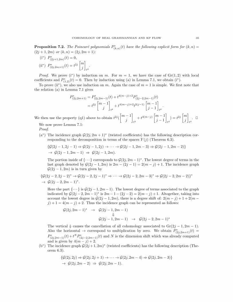
COHOMOLOGY OF REAL GRASSMANNIAN AND KP FLOW 35
Proposition 7.2. The Poincare polynomials P ∗(k,n)(t) have the following explicit form for (k, n) =
(2j + 1, 2m) or (k, n) = (2j, 2m+ 1):
(i∗) P ∗(2j+1,2m)(t) = 0,
(ii∗) P ∗(2j,2m+1)(t) = t2j[mj
]t4
.
Proof. We prove (i∗) by induction on m. For m = 1, we have the case of Gr(1, 2) with localcoefficients and P ∗(1,2)(t) = 0. Then by induction using (a) in Lemma 7.1, we obtain (i∗).
To prove (ii∗), we also use induction on m. Again the case of m = 1 is simple. We first note thatthe relation (a) in Lemma 7.1 gives
P ∗(2j,2m+1) = P ∗(2j,2m−1)(t) + t4(m−j)+2P ∗(2j−2,2m−1)(t)
= t2j[m− 1j
]t4
+ t4(m−j)+2t2(j−1)
[m− 1j − 1
]t4.
We then use the property (q1) above to obtain t2j(
[m− 1j
]t4
+ t4(m−j)[m− 1j − 1
]t4
) = t2j[mj
]t4
.
We now prove Lemma 7.1:Proof.
(a∗) The incidence graph G(2j, 2m+ 1)∗ (twisted coefficients) has the following description cor-responding to the decomposition in terms of the spaces Y (j) (Theorem 6.3).
{G(2j − 1, 2j − 1)⇒ G(2j − 1, 2j)→ · · · → G(2j − 1, 2m− 3)⇒ G(2j − 1, 2m− 2)}→ G(2j − 1, 2m− 1) ⇒ G(2j − 1, 2m).
The portion inside of {· · · } corresponds to G(2j, 2m−1)∗. The lowest degree of terms in thelast graph denoted by G(2j − 1, 2m) is 2m− (2j − 1) = 2(m− j) + 1. The incidence graphG(2j − 1, 2m) is in turn given by
{G(2j − 2, 2j − 2)∗ → G(2j − 2, 2j − 1)∗ ⇒ · · · → G(2j − 2, 2m− 3)∗ ⇒ G(2j − 2, 2m− 2)}∗
→ G(2j − 2, 2m− 1)∗.
Here the part {· · · } is G(2j− 1, 2m− 1). The lowest degree of terms associated to the graphindicated by G(2j − 2, 2m− 1)∗ is 2m− 1− (2j − 2) = 2(m− j) + 1. Altogether, taking intoaccount the lowest degree in G(2j − 1, 2m), there is a degree shift of: 2(m− j) + 1 + 2(m−j) + 1 = 4(m− j) + 2. Thus the incidence graph can be represented as follows:
G(2j, 2m− 1)∗ → G(2j − 1, 2m− 1)⇓
G(2j − 1, 2m− 1) → G(2j − 2, 2m− 1)∗
The vertical ⇓ causes the cancellation of all cohomology associated to Gr(2j − 1, 2m − 1).Also the horizontal → correspond to multiplication by zero. We obtain P ∗(2j,2m+1)(t) =
P ∗(2j,2m−1)(t) + tNP ∗(2j−2,2m−1)(t) and N is the dimension shift which was already computed
and is given by 4(m− j) + 2.(b∗) The incidence graph G(2j+1, 2m)∗ (twisted coefficients) has the following description (The-
orem 6.3).
{G(2j, 2j)⇒ G(2j, 2j + 1)→ · · · → G(2j, 2m− 4)⇒ G(2j, 2m− 3)}→ G(2j, 2m− 2) ⇒ G(2j, 2m− 1).
36 LUIS CASIAN AND YUJI KODAMA∗
The part {· · · } corresponds to G(2j + 1, 2m − 2)∗. The lowest degree of the terms in thechain complex corresponding to G(2j, 2m− 1) is 2m− 1− 2j = 2(m− j)− 1. The incidencegraph G(2j, 2m− 1) is in turn given by
{G(2j − 1, 2j − 1)∗ ⇒ G(2j − 1, 2j)∗ → · · · ⇒ G(2j − 1, 2m− 4)∗ → G(2j − 1, 2m− 3)∗}⇒ G(2j − 1, 2m− 2)∗.
The part {· · · } corresponds to G(2j, 2m − 1). The lowest degree of the terms in G(2j −1, 2m − 2)∗ is 2m − 2 − 2j + 1 = 2(m − j) − 1. Altogether we have a degree shift of2(m− j)− 1 + 2(m− j)− 1 = 4(m− j)− 2.
We thus have a graph that can be indicated by the diagram:
G(2j + 1, 2m− 2)∗ → G(2j, 2m− 1)⇓
G(2j, 2m− 1) → G(2j − 1, 2m− 2)∗.
This gives the recursive formula. The value of r is 4(m− j)− 2.(c∗) The incidence graph G(2j, 2m)∗ has the following description:
{G(2j − 1, 2j − 1)⇒ G(2j − 1, 2j)→ · · · → G(2j − 1, 2m− 3)⇒ G(2j − 1, 2m− 2)}→ G(2j − 1, 2m− 1).
This then can be represented as:
G(2j, 2m− 1)∗ → G(2j − 1, 2m− 1).
This gives rise to (c∗).(d∗) The incidence graph G(2j + 1, 2m+ 1)∗ has the following description:
{G(2j, 2j)⇒ G(2j, 2j + 1)→ · · · → G(2j, 2m− 2)⇒ G(2j, 2m− 1)}→ G(2j, 2m).
This then can be represented as
G(2j + 1, 2m)∗ → G(2j, 2m).
From here (d∗) follows.
This completes the proof.Similarly, we can derive the formulas for P ∗(2j,2m) and P ∗(2+1j,2m+1)(t).
Proposition 7.3. We have
(iii∗) P ∗(2j+1,2m+1)(t) = t2(m−j)[mj
]t4
,
(iv∗) P ∗(2j,2m)(t) = (t2j + t2(m−j))
[mj
]t4
.
7.2. The polynomials P(k,n)(t). Let us note the following Lemma for the additional recursionrelations of the Poincare polynomials.
Lemma 7.4. The polynomials P(k,n)(t) satisfy
(a) P(2j,2m+1)(t) = P(2j,2m)(t) + t2(m−j)+1P ∗(2j−1,2m)(t),
(b) P(2j+1,2m)(t) = P(2j+1,2m−1)(t) + t2(m−j)−1P ∗(2j,2m−1)(t),
(c) P(2j,2m)(t) = P(2j,2(m−1))(t) + t4(m−j)P(2j−2,2(m−1))(t),
(d) P(2j+1,2m+1)(t) = P(2j+1,2m−1)(t) + t4(m−j)P(2j−1,2m−1)(t).

COHOMOLOGY OF REAL GRASSMANNIAN AND KP FLOW 37
Before going through the proof, notice that this gives rise to explicit formulas for the polynomialsP(k,n)(t).
Theorem 7.5. We have the explicit form of the Poincare polynomials P(k,n)(t),
(i) P(2j,2m)(t) = P(2j,2m+1)(t) = P(2j+1,2m+1)(t) =
[mj
]t4
(ii) P(2j+1,2m)(t) = (1 + t2m−1)
[m− 1j
]t4
Proof. We use (c) of Lemma 7.4 and induction on m. We then can rewrite this recursive formulaas [
m− 1j
]t4
+ t4(m−j)[m− 1j − 1
]t4.
By the property (q1) above, this is just
[mj
]t4
. Using (a) of Lemma 7.4 and (i∗) of Proposition 7.2
we have P(2j,2m+1)(t) = P(2j,2m)(t) + t2(m−j)+1P ∗(2j−1,2m)(t) = P(2j,2m)(t). Using (d) of Lemma 7.4
and induction on m, we have P(2j+1,2m+1)(t) = P(2j+1,2m−1)(t) + t4(m−j)P(2j,2m−1)(t). This gives[m− 1j
]t4
+ t4(m−j)[m− 1j − 1
]t4,
which again corresponds to
[mj
]t4
.
Finally we use (b) of Lemma 7.4 and (ii∗) of Proposition 7.2 to obtain[m− 1j
]t4
+ t2m−1
[m− 1j
]t4,
which gives (2).We now prove Lemma 7.4.Proof.
(a) We have a graph of the form,
{G(2j − 1, 2j − 1)∗ → G(2j − 1, 2j)∗ ⇒ · · · → G(2j − 1, 2m− 2)∗ ⇒ G(2j − 1, 2m− 1)∗}→ G(2j − 1, 2m)∗.
The part {· · · } corresponds to G(2j, 2m). The lowest degree of the terms in the last graphdenoted by G(2j − 1, 2m− 1) is 2m − 2j + 1 = 2(m − j) + 1. We then have a graph whichcan be summarized as follows:
G(2j, 2m) → G(2j − 1, 2m)∗.
From here P(2j,2m+1) = P(2j,2m)(t) + trP ∗(2j−1,2m)(t) follows and r = 2(m− j) + 1.
(b) We have:
{G(2j, 2j)∗ → G(2j, 2j)∗ ⇒ · · · → G(2j, 2m− 3)∗ ⇒ G(2j, 2m− 2)∗}→ G(2j, 2m− 1)∗.
The portion inside {· · · } corresponds to G(2j+ 1, 2m− 1)∗. We then end up with a diagramthat can be summarized as:
G(2j + 1, 2m− 1) → G(2j, 2m− 1)∗.
The lowest degree in the chain complex corresponding to G(2j, 2m−1)∗ is then: 2(m−j)−1

38 LUIS CASIAN AND YUJI KODAMA∗
(c) The incidence graph G(2j, 2m) has the following description (Theorem 6.3).
{G(2j − 1, 2j − 1)∗ → G(2j − 1, 2j)∗ ⇒ · · · → G(2j − 1, 2m− 4)∗ ⇒ G(2j − 1, 2m− 3)∗}→ G(2j − 1, 2m− 2)∗ ⇒ G(2j − 1, 2m− 1)∗.
The portion inside of {· · · } corresponds to G(2j, 2m− 2). The lowest degree of the terms inthe last graph denoted by G(2j − 1, 2m− 1) is 2m − 2j = 2(m − j). The incidence graphG(2j − 1, 2m− 1)∗ is in turn given by
{G(2j − 2, 2j − 2)⇒ G(2j − 2, 2j − 1)→ · · · → G(2j − 2, 2m− 4)⇒ G(2j − 2, 2m− 3)}→ G(2j − 2, 2m− 2).
Here the part {· · · } is now G(2j − 1, 2m− 2)∗. The lowest degree of terms associated to thegraph indicated by G(2j − 2, 2m− 2)∗ is 2m− 2− (2j − 2) = 2(m− j). Altogether, takinginto account the lowest degree in G(2j − 2, 2m− 2), there is a degree shift of: 4(m− j). Wethus have a graph that can be indicated by the diagram:
G(2j, 2m− 2) → G(2j − 1, 2m− 2)∗
⇓G(2j − 1, 2m− 2)∗ → G(2j − 2, 2m− 2)
From here we obtain the recursive formula.(d) We start with the corresponding graph that can be represented by a diagram:
G(2j + 1, 2m− 1) → G(2j, 2m− 1)∗
⇓G(2j, 2m− 1)∗ → G(2j − 1, 2m− 1)
The lowest degree in the piece corresponding to G(2j − 1, 2m− 1) is 4(m−j). This becomesthe formula P(2j+1,2m+1)(t) = P(2j+1,2m−1)(t) + t4(m−j)P(2j,2m−1)(t).
This completes the proof of Lemma 7.4.
Remark 7.1. We note the similarity in the formulae of the Poincare polynomials for the real andcomplex Grassmannians. That is, in the case of (i) in Theorem 7.5, we have
P(k,n)(t) = PC(bk/2c,bn/2c)(t
2).
Also, in particular, if we take the limit n → ∞ for the case |t| < 1, we have for both cases (i) and(ii)
P(k,∞)(t) = PC(bk/2c,∞) =
bk/2c∏j=1
1
1− t4j.
This is a consequence of the structure of the cohomology ring of the Grassmannians in terms of thecharacteristic classes (see for example [3, 24]): It is well known that the real cohomology ring of thecomplex Grassmannian Gr(k, n,C) can be described by
H∗(Gr(k, n,C),R) ∼=R[c1, . . . , cn−k, c1, . . . , ck]
{c · c = 1},
where c := 1 + c1 + · · ·+ cn−k and ci = 1 + c1 + · · ·+ ck with the Chern classes cj ’s defined by
cj ∈ H2j(Gr(k, n,C),R).
The Poincare polynomial PC(k,n)(t) is then given by
PC(k,n)(t) =
[nk
]t2
=
k−1∏j=0
1− t2(n−j)
1− t2(k−j) .

COHOMOLOGY OF REAL GRASSMANNIAN AND KP FLOW 39
In particular, for the classifying space BU(k) as the infinite Grassmannian Gr(k, n,C) with n =∞,the cohomology ring is given by
H∗(BU(k),R) ∼= R[c1, c2, . . . , ck], with cj ∈ H2j(BU(k),R).
and the Poincare polynomial becomes the series given by
PC(k,∞)(t) =
k∏j=1
1
1− t2j.
For the classifying space BO(k) as the infinite Grassmannian Gr(k,∞), the cohomology ring isknown to be
H∗(BO(k),R) ∼= R[p1, p2, . . . , pbk/2c],
where the generators of the ring are given by the Potrjagin classes pj ∈ H4j(Gr(k, n),R). ThePoincare series of BO(k) is
P(k,∞)(t) =
bk/2c∏j=1
1
1− t4j= limn→∞
P(k,n)(t),
where the limit of course make sense for |t| < 1.
8. The Fq points on Gr(k, n) and the Poincare polynomials
Here we first introduce the weighted Schubert cell where the weight is given by the qη(wσ) (andqη(wσ)∗) defined in subsection 6.3. Then we define a polynomial p(k,n)(q) (and p∗(k,n)(q)) from the
incidence graph G(k, n) (and G(k, n)∗) based on the weights of the Schubert cells. It turns out thatthe polynomial p(k,n)(q) is related to the number of points on Gr(k, n) over the finite field Fq, andalso related to the Poincare polynomials P(k,n)(t) found in the previous section. The point hereis that the notion of the weighted Schubert cells gives a simple method to compute the Poincarepolynomials and the Fq points on Gr(k, n).
Remark 8.1. As in the case of the Toda-flow for the real flag variety discussed in [8], those polynomialsp(k,n)(q) can be computed by counting the number of blow-ups along the KP flow.
8.1. The q-weighted Schubert cells. Let us first recall that the Schubert cell (σ1, . . . , σk) can be
identified as an element wσ in S(k)n . Hence the vertices of the incidence graph G(k, n) correspond to
certain minimal length Weyl group representatives wσ. As shown in subsection 6.3, given L localsystem on Gr(k, n) certain powers of q can be associated to each vertex wσ. Since there are onlytwo local systems two consider, we can simplify the notation of [8], and just denote by qη(wσ) thepower of q assigned in the case when L is constant and qη(wσ)∗ the power of q in the case when L istwisted. We then associate powers qη(wσ) to each vertex wσ of G(k, n) and powers qη(wσ)∗ to eachvertex wσ of G(k, n)
∗. We call the Schubert cells Xwσ with those powers qη(w) the weighted Schubert
cells, denoted by (wσ, qη(wσ)) for each wσ ∈ S(k)
n .Here we consider only the η(w) (the η(w)∗ can be treated in a similar way). Let us first define
the following set of weighted vectors.
(a) For odd k, {ej(q) = (Ej ; q
b j2 c) : j = 1, . . . , n}.
(i.e. the weights are assigned as (1, q, q, q2, q2, . . . , qbn2 c)),

40 LUIS CASIAN AND YUJI KODAMA∗
(b) For even k, {ej(q) = (Ej ; q
b j−12 c) : j = 1, . . . , n
}.
(i.e. the weights are assigned as (1, 1, q, q, . . . , qbn−12 c)).
This is a q-deformation of the signed vector ej , and the sign for each vector Ej is given by settingq = −1. Then we can find the explicit form of the η(wσ).
Lemma 8.1. The function η(wσ) with the representation wσ = (σ1, . . . , σk) is given by
η(wσ) =k∑j=1
bσj − j2c if k = odd,
η(wσ) =k∑j=1
bσj − j − 1
2c if k = even.
To show this, we note that the η(wσ) satisfies the following conditions which uniquely determineη(wσ) for given Schubert cell wσ = (σ1, . . . , σk).
(i) To the top cell e = (1, 2, . . . , k) we associate η(e) = 0.(ii) If two Schubert cells w and w′ are joined by ⇒, i.e. w ⇒ w′, then η(w) = η(w′).(iii) If two Schubert cells w and w′ are joined by → (not ⇒), then η(w′) = η(w) + 1.
We then define a polynomial p(k,n)(q) as an alternating sum,
p(k,n)(q) :=∑
w∈S(k)n
(−1)`(w)qη(w)
We now offer a direct construction of the polynomials p(k,n)(q) which leads to their direct calcu-lation. An alternative way to proceed is through arguments similar to those leading to the recursiveformulas for Poincare polynomials. We have the following Theorem:
Theorem 8.2. The polynomials p(k,n)(q) take the forms,
p(2j,2m)(q) = p(2j,2m+1)(q) = p(2j+1,2m+1)(q) =
[mj
]q2
p(2j+1,2m)(q) = (1− qm)
[m− 1j
]q2.
Proof. Let us first consider the case Gr(2j, 2m). In this case we have{(E1; 1), (E2; 1), (E3, q), (E4; q), . . . , (E2m−1; qm−1), (E2m; qm−1)
}.
We compute p(2j,2m)(q) by computing all wedge products (σ1, · · · , σ2j) ↔ eσ1(q) ∧ · · · ∧ eσ2j
(q). It
is immediate that if a cell contains only one term from a pair {(E2i−1; qi−1), (E2i; qi−1)}, then this
cell is canceled by the cell containing the same terms except the term from the pair replaced by theother one. Thus the cells which contribute to p(2j,2m)(q) are given by the wedge products containing
pairs {(E2i−1; qi−1), (E2i, qi−1)} for some i, i.e.(
E2a1−1 ∧ E2a1 ∧ · · · ∧ E2aj−1 ∧ E2aj ; qj(j−1)+4|Y (a)|
).
Here Y (a) represents the Young diagram corresponding to (a1, . . . , aj), and 4 implies that each boxin Y (a) consists of 2× 2 cube of the boxes for the original Young diagram Yλ with
λ = (2(a1 − 1) + 1, 2(a1 − 1) + 2, . . . , 2(aj − j) + 2j − 1, 2(aj − j) + 2j) .
Since the generating function of the number of cells in Gr(j,m) is given by (2.2), we obtain theformula p(2j,2m)(q).

COHOMOLOGY OF REAL GRASSMANNIAN AND KP FLOW 41
Now let us consider the case Gr(2j, 2m+ 1). In this case we have,{(E1; 1), (E2; 1), . . . , (E2m−1; qm−1), (E2m; qm−1), (E2m+1; qm)
}.
It is easy to see that if a cell contains E2m+1 in 2j-wedge product, then this cell has no contributionin p(2j,2m+1)(q). Then the situation is the same as the case Gr(2j, 2m+ 1). A similar argument canbe applied for the case of Gr(2k + 1, 2n+ 1) (in this case, all the terms containing E1 vanish).
Finally we consider the case Gr(2j + 1, 2m). We start with{(E1; 1), (E2; q), (E3; q), . . . , (E2m−2; qm−1), (E2m−1; qm−1), (E2m; qm)
}.
We note that the cells containing both E1 and E2m have no contribution. There are two types ofcells which contribute; (i) those consisting of E1 and pairs {E2i, E2i+1} of the same degree qi, and(ii) those consisting of E2n and pairs of the same degrees. The first case (i), i.e. without E2m, givesthe same polynomial as in the case Gr(2j + 1, 2m − 1). The second case (ii), i.e. without E1, wehave the same polynomial times −qm due to the degree of E2m and (−1)l(w) = (−1)2m−1. We thusobtain the result for p(2j+1,2m)(q).
Remark 8.2. The polynomials p(k,n)(q) in Theorem 8.2 are related to the Poincare polynomialsP(k,n)(t) found in Theorem 7.5.
(a) For Gr(k, n) with (k, n) = (2j, 2m) or (2j, 2m+1) or (2j+1, 2m+1), the Poincare polynomialis given by P(k,n)(t) = p(k,n)(q = t2), i.e.
P(k,n)(t) =
[mj
]t4
=
j−1∏i=0
1− t4(m−i)
1− t4(j−i) .
For example, P(2,4)(t) = P(2,5)(t) = P(3,5)(t) = 1 + t4.(b) For Gr(k, n) with (k, n) = (2j + 1, 2m), P(k,n)(t) is given by
P(k,n)(t) = (1 + t2m−1)
[m− 1j
]t4.
Namely, the factor (1 − qm) in the polynomial p(k,n)(q) is replaced by (1 + t2m−1) and[m− 1j
]q2
with q = t2. For example, p(3,6)(q) = (1− q3)
[21
]q2
and P(3,6)(t) = (1 + t5)(1 +
t4) = 1 + t4 + t5 + t9.
Example 8.1. Following the constructive arguments in the proof of Theorem 8.2, we directly findthe polynomials p(k,n)(q) for the cases Gr(4, 8) and Gr(5, 12):
(a) For Gr(4, 8), we have the following cells which contribute the polynomial p(4,8)(q),
(1, 2, 3, 4) = e,(1, 2, 5, 6) = s4s5s3s4,(1, 2, 7, 8) = s6s7s5s6s4s5s3s4,(3, 4, 5, 6) = s2s3s1s2s4s5s3s4,(3, 4, 7, 8) = s2s3s1s2s6s7s5s6s4s5s3s4,(5, 6, 7, 8) = s4s5s3s4s2s3s1s2s6s7s5s6s4s5s3s4
Here the cells are represented by the elements of S(4)8 . Then the polynomial is given by
p(4,8)(q) = 1 + q2 + 2q4 + q6 + q8 =
[42
]q2.

42 LUIS CASIAN AND YUJI KODAMA∗
The Young diagrams of those cells are given by
(1, 2, 3, 4) = ∅, (1, 2, 5, 6) = , (1, 2, 7, 8) =
(3, 4, 5, 6) = , (3, 4, 7, 8) = , (5, 6, 7, 8) =
Note here that the box gives the unit for those diagrams and each diagram representsthe Pontrjagin class pj ∈ H4j(Gr(4, 8),R) for j = 1, 2, and this explains the relation,
p(4,8)(q) = |Gr(2, 4,Fq2)|.Then the cohomology ring may be expressed by
H∗(Gr(4, 8),R) ∼=R[p1, p2, p1, p2]
{p · p = 1},
where p = 1 + p1 + p2 and p = 1 + p1 + p2.(b) For Gr(5, 12), we have the contributing cells containing either E1 or E12,
(1, 2, 3, 4, 5) (2, 3, 4, 5, 12)(1, 2, 3, 6, 7) (2, 3, 6, 7, 12)(1, 2, 3, 8, 9) (2, 3, 8, 9, 12)(1, 2, 3, 10, 11) (2, 3, 10, 11, 12)(1, 4, 5, 6, 7) [1 → 12] (4, 5, 6, 7, 12)(1, 4, 5, 8, 9) (4, 5, 8, 9, 12)(1, 4, 5, 10, 11) (4, 5, 10, 11, 12)(1, 6, 7, 8, 9) (6, 7, 8, 9, 12)(1, 6, 7, 10, 11) (6, 7, 10, 11, 12)(1, 8, 9, 10, 11) (8, 9, 10, 11, 12)
The cells in the left hand side gives 1 + q2 + 2q4 + 2q6 + 2q8 + q10 + q12 = (1 − q10)(1 −q8)/(1− q4)(1− q2), and those in the right hand side gives −q6 times the same polynomial,i.e.
p(5,12)(q) = (1− q6)
[52
]q2.
The Young diagrams for the cells in the left column are given by
∅
The Young diagrams of the cells in the right column are given by the above ones combinedwith the first cell in the right column,
(2, 3, 4, 5, 12) = .
That is, we have, from the second cell,
Note again that those cells are expressed by the diagrams and . Each diagram of
divisible by represents the Pontrjagin class pj ∈ H4j(Gr(5, 12),R), and the hook diagrammay correspond to an extra element, say r, of degree 11 with the property r2 = 0. It thenmay be natural to conjecture that the cohomology ring of Gr(5, 12) has the structure,
H∗(Gr(5, 12),R) ∼=R[p1, p2, p3, p1, p2, r]
{p · p = 1, r2},
where p = 1 + p1 + p2 + p3, and p = 1 + p1 + p2.

COHOMOLOGY OF REAL GRASSMANNIAN AND KP FLOW 43
The proof of the following Proposition is similar to the calculation of P ∗(2j,2m+1)(t), P∗(2j+1,2m+1)(t)
and is omitted.
Proposition 8.3. We have:
p∗(2j,2m+1)(q) = qj[mj
]q2
p∗(2j+1,2m+1)(q) = qm−j[mj
]q2
8.2. The number of Fq-points on Gr(k, n). The main goal of this section is to show that theFq-points on the Grassmannian Gr(k, n) is given by
|Gr(k, n)Fq | = qr |p(k,n)(q)|where r is given by r = k(n− k)− deg (p(k,n)(q)).
In order to calculate |Gr(k, n)Fq |, we first introduce the complexification Gr(k, n)C of the realGrassmannian Gr(k, n), which is not the complex Grassmannian Gr(k, n,C), but rather, a Zariskiopen subset of Gr(k, n,C) having the same homotopy type as Gr(k, n). So, for instance the com-plexification of RP 1 = Gr(1, 2) is not Gr(1, 2,C) which is CP 1, but rather, the set of all lines inC2 = {(x, y)} such that x2 + y2 6= 0. This is an open subset of CP 1 which has the homotopy typeof a circle.
Definition 8.1. We fix a real vector subspace of dimension k, V ⊂ Rn and its complexification VC =V ⊕R
√−1V . The group SOn(R) acts transitively on Gr(k, n) but the orbit SOn(C) ·VC of the vector
space VC does not exhaust all of Gr(k, n,C). We define this orbit as the complexification of Gr(k, n),and denoted by Gr(k, n)C. The real Grassmanian Gr(k, n) can then be described as K/L∩K, whereK = SOn(R) and the Levi factor L of a maximal parabolic subgroup containing the Borel subgroup Bof upper triangular matrices in SLn(R) and the complexification is K(C)/L(C)∩K(C) = SOn(C)·VCwhich has the same homotopy type as Gr(k, n).
This naturally extends to other semi-simple Lie groups. In brief, if G = KAN (Iwasawa de-composition) and P = LN is a maximal parabolic with Levi factor L containing a maximally splitCartan subgroup H = TA , then we have G/P ∼= K/K ∩ L and the complexification will beK(C)/L(C) ∩K(C).
Example 8.2. Consider RPn−1. If we fix V a one dimensional vector subspace of Rn. Then theSO(n,C) orbit containing VC can be described as the set of all lines in Cn, denoted by C(x1, · · ·xn),such that x2
1 +· · ·x2n 6= 0. This is an open subset Gr(1, n)C of the Grassmanian Gr(1, n,C) = CPn−1.
Example 8.3. Let us consider Gr(2, 4). Using the Plucker embedding as in Example 2.2, thecomplexification can be explicitly described as follows.
Gr(2, 4)C =
{C(z1, z2, z3, w1, w2, w3) :
z21 + z2
2 + z23 − w2
1 − w22 − w2
3 = 0,z2
1 + z22 + z2
3 6= 0
}.
This is an open subset of Gr(2, 4,C). This formula is useful for counting the Fq-points on Gr(k, n)(see below).
We consider Fq an algebraic closure of a field Fq with q elements, and consider Grassmannian
varieties Gr(k, n,Fq). As a set of points this is the set of all the k-dimensional subspaces of Fnq .
However the Gr(k, n,Fq) is the Fq-analogue of the standard complex Grassmannian variety
Gr(k, n,C). Here we are interested instead in the Fq-counterparts of the complexifications Gr(k, n)Cof real Grassmannians in counting their Fq-points.
Assume that q is a power of a prime number p 6= 2 such that in Fq the polynomial x2 + 1 is
reducible i.e.√−1 ∈ Fq. If p has the form p = 4k + 1 with k an integer, this will be the case
44 LUIS CASIAN AND YUJI KODAMA∗
e.g. q = 5. We then consider the analogue of Gr(k, n) over Fq, that is, the Zariski open subset
Gr(k, n)Fq of Gr(k, n,Fq) and then the corresponding Fq points. Then we have the following results
for |Sn(Fq)|, the number of Fq-points on Sn:
(a) For n = 2m− 1, we have
|S2m−1(Fq)| = qm−1(qm − 1) .
(b) For n = 2m, we have
|S2m(Fq)| = qm(qm + 1) .
This can be obtained as follows: Let us first consider the case n = 1, i.e.
S1(Fq) = {(x, y) ∈ F2q : x2 + y2 = 1} .
Then using the formulae for the stereographic projection; x = 2uu2+1 , y = u2−1
u2+1 with y 6= 1 and
{u ∈ Fq : u2 + 1 6= 0}. Since√−1 ∈ Fq, we have 2 points in {u2 + 1 = 0}. Counting the point
(0, 1), the north pole, we have |S1(Fq)| = q − 2 + 1 = q − 1. Now consider the case n = 2, we have
x = 2u1
u21+u2
2+1, y = 2u2
u21+u2
2+1, z =
u21+u2
2−1
u21+u2
2+1with z 6= 1 and {(u1, u2) ∈ F2
q : u21 + u2
2 + 1 6= 0}. This
gives q2 − (q − 1) points (note (q − 1) is the number of points in u21 + u2
2 + 1 = 0). We now addthe points of the north pole (x, y, 1) with x2 + y2 = 0. This gives 2(q − 1) + 1, where 2(q − 1) forx = ±
√−1y 6= 0 and 1 for (0, 0, 1). Then we have |S2(Fq)| = q2 − (q − 1) + 2(q − 1) + 1 = q(q + 1).
Using the induction, one can show that the number of points in the north pole is given by
(8.1)
{ |{(x1, . . . , x2m−1) ∈ F2m−1q : x2
1 + · · ·+ x22m−1 = 0}| = q2m−2,
|{(x1, . . . , x2m) ∈ F2mq : x2
1 + · · ·+ x22m = 0}| = q2m−1 + qm − qm−1.
Then one can obtain the above formulae for |Sn(Fq)|.
Example 8.4. We consider the analogue of RPn−1 over Fq, that is, the Zariski open subsetGr(1, n)Fq of Gr(1, n,Fq). Recall that we have the Schubert decomposition,
CPn−1 = Gr(1, n,C) = {(∗, . . . , ∗, 1)} t {(∗, . . . , ∗, 1, 0)} t · · · t {(1, 0, . . . , 0)} ,
and we have |Gr(1, n,Fq)| = [n]q = 1 + q+ · · ·+ qn−1. To find |Gr(1, n)Fq |, the number of Fq points
on RPn−1, we have to remove the points in the Schubert cells given by
{(x1, . . . , xk, 1, 0, . . . , 0) ∈ Fnq : x21 + · · ·+ x2
k + 1 = 0} k = 1, . . . , n− 1.
Since√−1 ∈ Fq, those sets are equivalent to Sk−1 on Fq whose points can be counted from the
formulae above. Thus we get
(a) For n = 2m,
|Gr(1, 2m)Fq | = qm−1(qm − 1) .
(b) For n = 2m+ 1,
|Gr(1, 2m+ 1)Fq | = q2m .
As was shown in Proposition 8.2, those polynomials are related to p(1,n)(q), i.e. p(1,2m)(q) = 1− qmand p(1,2m+1)(q) = 1, and we have the form,
|Gr(1, n)Fq | = qr|p(1,n)(q)|.
Example 8.5. We now consider Gr(2, 4). As in Example 2.2, Gr(2, 4) becomes, via the Pluckerembedding, the set of one dimensional isotropic vector spaces in R6. We then have, as in Example8.3, the following description of the Fq points of the variety we are studying
Gr(2, 4)Fq = {(x1, x2, x3, y1, y2, y3) ∈ F6q : x2
1 + x22 + x2
3 − y21 − y2
2 − y23 = 0, x2
1 + x22 + x2
3 6= 0}.

COHOMOLOGY OF REAL GRASSMANNIAN AND KP FLOW 45
Since√−1 ∈ Fq, we can transform the equation x2
1 + x22 + x2
3− y21 − y2
2 − y23 = 0 giving isotropy into
x21 + x2
2 + x23 + y2
1 + y22 + y2
3 = 0. The number of solutions of x21 + x2
2 + x23 + y2
1 + y22 + y2
3 = 0 isgiven by q5 + q3− q2 (see (8.1)). We now must subtract those points for which x2
1 +x22 +x2
3 = 0 andy2
1 + y22 + y2
3 = 0. From (8.1), one can see that there are q2 solutions of x21 + x2
2 + x23 = 0. So with
an additional q2 solutions of y21 + y2
2 + y23 = 0, we end up with q5 − q4 + q3 − q2 = q2(q− 1)(q2 + 1).
We now divide by q − 1 to count the projectivization and obtain a total of q2(1 + q2) points.
Example 8.6. Using the formulae for |Sn(Fq)| for the case with√−1 ∈ Fq, one can write an
explicit formula giving the number of Fq points of finite Chevalley group SOn(Fq): First recall thatSOn+1(R)/SOn(R) ∼= Sn. Then one expects:
|SOn(Fq)| =n∏k=1
|Sn−k(Fq)| ,
which corresponds to the results [4]:
(a) For n = 2m,
|SO2m(Fq)| = 2qm(m−1)(q2 − 1)(q4 − 1) · · · (q2m−2 − 1)(qm − 1) .
(b) For n = 2m+ 1,
|SO2m+1(Fq)| = 2qm2
(q2 − 1)(q4 − 1) · · · (q2m − 1) .
In [8], we show that those polynomials p(q) = (q2 − 1)(q4 − 1) · · · (q2m−2 − 1)(qm − 1) and p(q) =(q2−1)(q4−1) · · · (q2m−1) are related to the cohomology of the real flag variety SLn(R)/B throughthe singular solutions (blow-ups) of the Toda lattice.
We assume that q is a power of a prime p , m is relatively prime to p and p 6= 2. Moreover, asbefore we assume that
√−1 ∈ Fq. As in [8] one has the following.
Proposition 8.4. The cohomology H∗(Gr(k, n)Fq ;Qm) has Frobenius eigenvalues of the form qi.
Proof. This follows from the arguments in [8] with almost no change. As can be seen from [9]or more directly by Remark 6.1 above, the incidence graph of Gr(k, n) is a subgraph of the flagmanifold. The Frobenius eigenvalues are still computed in terms of Hecke algebra operators as inSection 5 of [8] but the Weyl group elements in the expressions T−1
w−1 are restricted to a smallersubset corresponding to representatives of cells in a Grassmanian. This is also implicit in Section 9of [9] but notation is more convoluted.
One may also consider the spectral sequence associated to the fibration
(K ∩ L)(Fq) → (K)(Fq) → (K/L ∩K)(Fq)
This reduces the argument to the cases of K ∩ L and K over Fq. The case of K and L ∩K is justthe case discussed in [8] of the flag manifold.
We now recall that from the Lefschetz fixed point formula for Fr the alternating sum is given by∑s
(−1)sTr(
(Fr)∗|Hsc (Gr(k,n)Fq ;Qm)
)= |Gr(k, n)Fq |
By Poincare duality, H2k(n−k)−sc (Gr(k, n)Fq ; Qm) is the dual of Hs(Gr(k, n)Fq ;V) where V is the
dual of a constant sheaf. In the orientable cases we can replace V with Qm i.e. constant coefficients.

46 LUIS CASIAN AND YUJI KODAMA∗
8.3. Frobenius eigenvalues calculation. This calculation is based on section 9 of [9] or on Section6.1 [8] which is restricted to real split cases and has simpler notation. Frobenius eigenvalues qi
increase along a graph G(k, n) or G(k, n)∗
as described in (i),(ii), (iii) in Subsection 8.1.In terms of the action of the Hecke algebra in Lemma 3.5 of [23] , one must apply T−1
s+i =
q−1(Tsi + (1 − q)). Now ⇒ corresponds to case (e) and the Frobenius eigenvalue does not change.The case of → corresponds to (d2) and the Frobenius eigenvalue is multiplied by q.
By construction of the polynomial p(k,n)(q) we have∑s
(−1)sTr(
(Fr)∗|Hs(Gr(k,n)Fq ;Qm)
)= p(k,n)(q)
This leads to the following Proposition,
Proposition 8.5. We have
|Gr(k, n)Fq | = ±qk(n−k)−Dp(k,n)(q),
with D = deg(p(k,n)(q)).
Proof. We consider the cases with n =even (orientable case) and n =odd (non-orientable case):
(1) Assume that n is even. We use Poincare duality, H2k(n−k)−sc (Gr(k, n)Fq ; Qm) is the dual of
Hs(Gr(k, n)Fq ; Qm). This corresponds to considering the polynomial qk(n−k)p(k,n)(q−1). We
now used the formulas listed at the beginning of Section 7. We note that ifD = deg(p(k,n)(q))
then, according to these formulas qDp(k,n)(q−1) = ±p(k,n)(q). Hence we obtain∑
s(−1)sTr
((Fr)∗|Hsc (Gr(k,n)Fq ;;Qm)
)= |Gr(k, n)Fq | = ±qk(n−k)−Dp(k,n)(q).
(2) Assume that n is odd. By Poincare duality, H2k(n−k)−sc (Gr(k, n)Fq ; Qm) is the dual of
Hs(Gr(k, n)Fq ;L) where L is a twisted local system. We then have qk(n−k)p∗(k,n)(q−1). We
then use Proposition 8.3. We obtain qk(n−k)qrp(k,n)(q−1) where r = −j or r = m − j if
k = 2j, 2j + 1 and n = 2m+ 1.
This completes the proof.
References
[1] M. J. Ablowitz and H. Segur, Solitons and the inverse scattering transform, SIAM Studies in Applied Mathemat-
ics, (SIAM, Philadelphia/ 1981).[2] A. Bjorner and F. Brenti, Combinatorics of Coxeter Groups, GTM 231 (Springer, New York, 2005).[3] R. Bott and L. W. Tu, Differential forms in algebraic topology, (Springer-Verlag, New York) (1982).[4] R. Carter, Finite Groups of Lie Type, Conjugacy Classes and Complex Characters, Wiley Classical Library
Edition (1993).[5] L. Casian and Y. Kodama, Topology of the iso-spectral real manifold associated with the generalized Toda lattices
on semisimple Lie algebras, J. Phys. A: Math. Gen. 33 (2000) 1-14.[6] L. Casian and Y. Kodama, Blow-ups of the Toda lattices and their intersections with the Bruhat cells, Contem-
porary Math. 301 (2002) 283-310.[7] L. Casian and Y. Kodama, Compactification of the isospectral varieties of nilpotent Toda lattices, Surikaisekiken
Kokyuroku (RIMS Proceedings, Kyoto University), 1400 (2004) 39-87.[8] L. Casian and Y. Kodama, Toda lattice, cohomology of compact Lie groups and finite Chevalley groups, Invent.
Math. 165 (2006) 163-208.[9] L. Casian and R. Stanton, Schubert cells and representation theory, Invent. Math. 137 (1999) 461-539.
[10] S. Chakravarty and Y. Kodama, Classification of the line-solitons of KPII, J. Phys. A: Math. Theor. 41 (2008)275209 (33pp).
[11] S. Chakravarty and Y. Kodama, Soliton solutions of the KP equation and application to shallow water waves,
Stud. Appl. Math. 123 (2009) 83-151.

COHOMOLOGY OF REAL GRASSMANNIAN AND KP FLOW 47
[12] I. M. Gel’fand and V. V. Sarganova, Combinatorial geometries and torus strata on homogeneous compact mani-
folds, Russian Math. Surveys, 42:2 (1987) 133-168.
[13] W. Fulton and J. Harris, Representation Theory GTM 129 (Springer, New York, 1991).[14] F. R. Gantmacher, The theory of matrices, (Chelsea Publishing Company, New York, 1990)
[15] R Hirota, The Direct Method in Soliton Theory (Cambridge University Press, Cambridge, 2004)
[16] B. Iversen, Cohomology of sheaves, (Springer-Verlag, New York, 1986).[17] S. J. Jungking, Some computations of the homology of real Grassmannian manifolds, Master thesis at The
University of British Columbia, (September, 1979). (https://circle.ubc.ca/handle/2429/21381).
[18] B B Kadomtsev and V I Petviashvili, On the stability of solitary waves in weakly dispersing media Sov. Phys.Doklady, 15 (1970) 539-541.
[19] R. R. Kocherlakota, Integral Homology of Real Flag Manifolds and Loop Spaces of Symmetric Spaces, Advances
in mathematics 110,(1995), 1-46[20] Y. Kodama, KP solitons in shallow water, J. Phys. A: Math. Gen., 43 (2010) 434004 (54pp).
[21] Y. Kodama and J. Ye, Toda lattices with indefinite metric II: Topology of the iso-spectral manifolds, Physica D121 (1998) 89-108.
[22] D. Kadhdan and G. Luszig, Schubert varieties and Poincare duality, Proc. Symp. in Pure Math., AMS 36 (1980)
185-203.[23] G. Lusztig and D. Vogan, Singularities of Closures of K-orbits on Flag Manifolds, Invent. Math. 71 (1983)
365-379.
[24] J. W. Milnor and J. D. Stasheff, Characteristic classes, (Princeton University Press, Princeton), (1974).[25] T. Miwa, M. Jimbo and E. Date, Solitons: Differential equations, symmetries and infinite dimensional algebras,
(Cambridge University Press, 2000) Translated from the Japanese version published by Iwanami-Publication in
1993.[26] M. Sato, Soliton equations as dynamical systems on an infinite dimensional Grassmann manifolds, RIMS
Kokyuroku, 439 (1981) 30-46.
[27] H. Yeh, W. Li and Y. Kodama, Eur. Phys. J. Special Topics, 185 (2010) 97-111.
Department of Mathematics, Ohio State University, Columbus, OH 43210
E-mail address: [email protected]
Department of Mathematics, Ohio State University, Columbus, OH 43210E-mail address: [email protected]