arX

iv:h

ep-t

h/95

0403

7v1

7 A

pr 1

995

BRST COHOMOLOGY FOR 2D GRAVITY

Paul A. Blaga,

Department of Geometry

Liviu Tataru and Ion V. Vancea,

Department of Theoretical Physics,

Babes - Bolyai University of Cluj,

Romania

July 24, 2013

Abstract

The BRST cohomology group in the space of local functionals of the fields for the two-

dimensional conformally invariant gravity is calculated. All classical local actions (ghost

number equal to zero) and all candidate anomalies are given and discussed for our model.

1 Introduction

Gauge fields play a very important role in all theories which describe the fundamental interactions

[1]. The most efficient way to study the quantization and the renormalization of all gauge (local)

theories is given by the BRST transformations and by the so-called BRST cohomology [2, 3, 4].

Despite the fact that gravity could be introduced as a gauge theory associated with local Lorentz

invariance [5], its action has a different structure and it is difficult to connect it to a special form

of the Yang-Mills theory, known as the topological quantum field theory [6]. However, in the

BRST quantization framework the structure of the invariant action, the anomalies and the

Schwinger terms can be obtained in a purely algebraic way by solving the BRST consistency

conditions in the space of the integrated local field polynomials [7, 8]. This fact has been known

since the work of Wess and Zumino [9] and for a general gauge theory the general form of

these can be elegantly formulated in the BV formalism [3]. In this framework, the Wess-Zumino

consistency condition [7, 8] can be written as:

sA = (S,A) = 0 (1.1)

where S is the proper solution of the master equation, A are integrated local functionals and s is

the BRST nilpotent differential [7, 8, 10]. The solutions of (1.1) modulo the exact forms A = sB

can be organized in an abelian group H(s), the BRST cohomology group. We can introduce a

graduation in H(s) by the ghost number (gh = g) and we can decompose it in a direct sum of

subspaces with a definite ghost number:

H(s) = ⊕Hg(s) (1.2)

Anomalies are represented by cohomology classes ofH1(s), but it is often useful to computeHg(s)

for other values of g as well since H0 contains the BRST invariant action andH2(s)the Schwinger

terms. Besides, the whole H(s) could play an important role in solving and understanding the

descent equations [7, 8] and in the study of structure of the field configurations.

In this paper we are going to investigate the structure of H(s) for a class of two dimensional

models which are conformally invariant at the classical level. We will not characterize these

models by specific conformally invariant classical actions but we rather specify the field content

1

and the gauge invariances of the theory. We will try to obtain H(s) for a general framework

independent on the local classical action S0. Thus we are not going to introduce the antifields

[3, 2] which have the BRST transformations dependent on S0.

The paper is organized as follows: in Sect.2 we recall the field content and the gauge symmetries

of our model. In Sect.3 we give the equations which have to be solved in order to find out

invariant Lagrangians, anomalies and Schwinger terms. Sect.4 deals with the analysis of the

algebra of all fields and their derivatives. We shall show that A can be splitted in its contractive

part C and its minimal subalgebra M . In the minimal algebra we introduce, following [11] a very

convenient basis where the solution of (1.1) are very simple. At the end we give the structure

of all nontrivial sectors of H(s) and in Sect.5 we give some comments of our results.

2 Two-dimensional conformal gravity

Our main aim is to compute the BRST cohomology group for a class of two-dimensional models

which are conformally invariant at the classical level. We are not going to characterize these

models by the local classical action S0, but we will provide only the field contents and the

gauge invariance of the classical theory. Then we can define the BRST differential s and we

can compute the BRST cohomology group H∗(s) in the space of local functionals of the fields.

Thus, for ghost number zero, this group provides the most general local classical action S0. For

ghost number one, H1(s) gives us the most general local anomalies. In this paper we are not

going to take into account the antifields and we do not need the concrete form of the classical

action S0 which enters the BRST transformations.

The fields of our theory are the components of the 2D metric gµν = gνµ and the set of bosonic

scalar matter fields (X = XA, A = 1, . . . , D). It is convenient to replace the metric gµν by the

zweibein fields eaµ such that:

gµν = eaµe

bνηab (2.3)

where µ, ν = 0, 1, a, b = 0, 1 and ηab = (+,−) or by the moving frame

ea = eaµdx

µ (2.4)

2

The conformal properties of the two-dimensional spacetime are most conveniently described in

terms of light-cone coordinates:

x± =1√2(x0 ± x1)

and the differential operators∂

∂x±=

1√2

(

∂

∂x0± ∂

∂x1

)

(2.5)

For the moving frame one defines the one-forms:

e± =1√2(e0 ± e1) (2.6)

with the coefficients

e+ = (dx+ + h−−dx−)e++ (2.7)

e− = (dx− + h++dx+)e−− (2.8)

Here

h++ =e+−e++

h−− =e−+e−−

(2.9)

are the gauge fields which occur for the nonchiral Virasoro algebra. They can be expressed in

terms of the components of the metric gµν by using the definitions (2.3) and (2.4). The metric

becomes:

ds2 = gαβdxαdxβ (2.10)

where α, β = +,−. The components of the metric in light-cone frame read out as:

g±± =1

2(g00 ± 2g01 + g11)

g+− =1

2(g00 − g11) (2.11)

g−+ = g+−

and employing the zweibein

ds2 = ηabeaeb (2.12)

Thus, we can write the gauge fields as follows:

h±± =g±±

g+− +√g

(2.13)

3

with g = |det(gµν)|.The fields h±± are inert under local Lorentz (structure) group transformations and change

under diffeomorphisms (i.e., from one chart to another) in the following way:

h++ =(∂x′+/∂x−) + (∂x′−/∂x−)h′++(x′)

(∂x′+/∂x+) + (∂x′−/∂x+)h′++(x′)(2.14)

h−− =(∂x′−/∂x+) + (∂x′+/∂x+)h′−−(x′)

(∂x′−/∂x−) + (∂x′+/∂x−)h′−−(x′)(2.15)

Besides, the fields h±± remain invariant under the Weyl transformation gαβ → eσgαβ. The

conformal factors e++ and e−− carry entirely the local Lorentz group transformations and the

Weyl transformation. Thus, if we want to define a theory that is invariant under the local Weyl

transformations of the metric gαβ we have to work only with the fields h±± instead of the whole

metric gαβ

In the parametrization (2.7) and (2.8) of the moving frame, the structure group and Weyl

transformations are carried entirely by the conformal factors ǫ±±. Besides, upon general coordinate

transformations they change as

e++(x) =

[

∂x′+

∂x++∂x′−

∂x+h′++(x)

]

e′++ (x′) (2.16)

and

e−−(x) =

[

∂x′−

∂x−+∂x′+

∂x−h′−−(x)

]

e′−− (x′) (2.17)

Under a Weyl transformation, the fields h±± and the matter fields X remain invariant and the

conformal factors e++ and e−− change as:

e++(x) = e−σ

2 e′++ (x) (2.18)

e−−(x) = e−σ

2 e′−− (x)

Upon a general coordinate transformation they change as:

e++(x) = [∂x

′+

∂x++∂x

′−

∂x+h

′

++(x)]e′+

+ (x) (2.19)

e−−(x) = [∂x

′−

∂x−+∂x

′+

∂x−h,−−(x)]e

′−− (x) (2.20)

4

The geometric description, developed so far, provides the base for the description of the two-

dimensional theories which have local reparametrization ( diffeomorphism) as well as Weyl and

Lorentz invariance. Upon quantization, the whole theory must undergo the standard BRST

treatment ( or quantization) to control the degeneracies due to the local gauge transformations.

This will be done in the next section.

The matter field X = {Xµ} are scalar under the diffeomorphism, i.e., they have the following

transformation under a general coordinate transformation:

X(x) = X ′(x′). (2.21)

We will suppose that X(x) have the Weyl weight zero, i.e., they are invariant under the Weyl

transformation. In fact, in D dimensions the Weyl weight for X(x) is

w(X) = −D − 2

2

which is zero for D = 2.

3 BRST transformations of the model

The BRST transformations and the BRST differential can be obtained in general by simply

replacing the infinitesimal gauge parameters εα which occur in the gauge transformation:

δεϕi = Ri

αεα

by the ghosts cα(x):

sϕi = Riαc

α

The BRST transformations of the ghosts are defined by demanding that s should be nilpotent.

For an infinitesimal diffeomorphism we have

x′µ = xµ + εµ(x) (3.1)

with ε0 and ε1 infinitesimal arbitrary functions of x. Under the transformation (3.1) h±± change

as:

δh++ = h++(∂−ε− + h++∂−ε+) − (∂+ε

− + h++∂+ε+) − (ε+∂+ + ε−∂−)h++ (3.2)

δh−− = h−−(∂+ε+ + h−−∂+ε−) − (∂−ε

+ + h−−∂−ε−) − (ε−∂− + ε+∂+)h−−

5

where ∂+ = ∂/∂x+ and ∂− = ∂/∂x−.

The matter field X has the following transformation under the diffeomorphism (3.1):

δX = (ε+∂+ + ε−∂−)X (3.3)

From (3.1), (3.3), (3.3) we get the BRST transformations by simply replacing the infinitesi-

mal gauge parameters ε± by the diffeomorphism ghost ξ±. These transformations can be simpli-

fied if new ghost fields c± are introduced following the line of [11, 17, 19, 20]:

c± = ξ± + h∓∓ξ∓ (3.4)

Thus, the BRST transformations of h++, h−−, X are:

sh++ = ∂+c− − h++∂−c

− + c−∂−h++

sh−− = ∂−c+ − h−−∂+c

+ + c+∂+h−− (3.5)

sX = c+D+X + c−D−X

where:

D±X =1

1 − y(∂± − h±±∂∓)X =

1

1 − y∇±X (3.6)

y = h++h−−

The BRST transformations of the ghosts c± can be obtained from the nilpotency of s and the

fact that it commutes with ∂±. In this way we conclude that

sc± = c±∂±c± (3.7)

Under the Weyl transformation h++ and h−− remain invariant and only the conformal factors

e++ and e−− change.

In the framework of the BRST transformations, the search for invariant Lagrangian anoma-

lies and Schwinger terms can be done in a purely algebraic way, by solving the BRST consistency

condition in the space of integrated local polynomials [9, 12, 13]. This amounts to study the non-

trivial solutions of the equation

sA = 0 (3.8)

6

where A is an integrated local functional A =∫

d2f . The condition (3.8) translates into the

local descent equations [14]:

sω2 + dω1 = 0

sω1 + dω0 = 0 (3.9)

sω0 = 0

where ω2 is a 2-form with A =∫

ω2 and ω1, ω0 are local 1-forms, respectively 0-forms. It is well

known [12, 13, 16] that the descent equations terminate in the bosonic string or the superstring

in Beltrami or super-Beltrami parametrization always with a nontrivial 0-form ω0 and that their

integration is trivial:

ω1 = δω0; ω2 =1

2δ2ω0 (3.10)

where δ is a linear operator, which allows to express the exterior derivative d as a BRST com-

mutator

d = −[s, δ] (3.11)

This operator was introduced by Sorella for the Yang-Mills theory [14] and it was used for solving

the descent equations (3.10) for the bosonic string [12] and superstring [16] in the Beltrami and

super-Beltrami parametrization. It is easy to see that, once the last equation in the tower (3.10),

i.e.,

sω0 = 0 (3.12)

is solved, the rest of the equations from (3.10) can be solved with the help of the operator δ

with the solutions (3.10). Thus, due to the operator δ, the study of the cohomology ofs mod d is

essentially reduced to the study of the local cohomology of s which, in turn, can be systematically

analyzed by using different powerful techniques from the algebraic topology as the Sullivan and

Kunneth theorems, the spectral sequences [8], etc. Actually, as proven in [15] for the Yang-Mills

theory, the solutions obtained by utilizing the decomposition (3.10) turn out to be completely

equivalent to that based on the Russian formula[7].

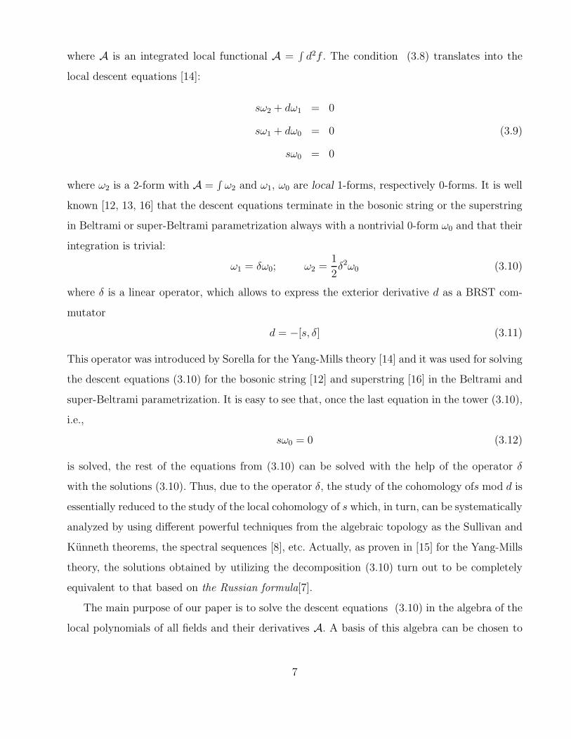
The main purpose of our paper is to solve the descent equations (3.10) in the algebra of the

local polynomials of all fields and their derivatives A. A basis of this algebra can be chosen to

7

consist of:

{∂p+∂

q−ψ, ∂

p+∂

q−c

±} (3.13)

where ψ = (X, h++, h−−) and p, q = 0, 1, 2, . . .. However, the BRST transformations of this basis

are quite complicated and contain many terms which can be eliminated in H(s). In the next

section we shall eliminate a part of this basis and introduce a new basis in which the action of

s is quite simple. *****

4 The structure of the fields algebra

The calculation of H(s) can be considerable simplified if we take into account that A as a free

differential algebra and make use of a very strong theorem due to Sullivan. A free differential

algebra is an algebra generated by a basis, endowed with a differential. The Sullivan’s theorem

tells us the following:

The most general free differential algebra A is a tensor product of a contractible algebra and

a minimal one

A minimal differential algebra M with the differential s is one for which sM ⊂ M+.M+

being the part of M in positive degree, i.e. M = C ⊕M+ and a contractible differential algebra

C is one isomorphic to a tensor product of algebras of the form Λ(x, sx).

On the other hand, due to Kunneth’s theorem the cohomology of A is given by the coho-

mology of its minimal part and we can say that the contractible part C can be neglected in the

calculation of H(s)

For our algebra, the construction of C and M is straightforward and we do not need any

general method to accomplish that. In fact, it is easy to see from the BRST transformations of

h±±, X, c± that the generators

∂p+∂

n−c

+, ∂p+∂

n−c

− (4.1)

with p = 0, 1, 2, . . . and n = 1, 2, . . . can be replaced by:

{∂p+∂

p−X, ∂

p+∂

p−φ, s∂

p+∂

p−φ, ∂

p±c

±} (4.2)

8

The Sullivan decomposition can be easily obtained from (4.2). Indeed, the contractible sub-

algebra is generated by:

{∂p+∂

p−h±±, s(∂

p+∂

p−h±±)} (4.3)

and the minimal subalgebra M by:

{∂p+∂

p−X, ∂

p±c

±} (4.4)

Now, to calculate the cohomology H(s) we take into account only the basis (4.4). Never-

theless, this basis is not convenient since the differential s has a complicated action on it. The

investigation of the BRST cohomology, i.e., the solution of (3.12) is considerable simplified

by using an appropriate new basis substituting the fields(X, c±) and their derivatives. The con-

struction of this new basis is a crucial step towards the calculation of H(s). This new basis has

been proposed by Brandt, Troost and Van Proeyen [11] and it is basically intended to substitute

one by one the elements of the basis (4.4) by:

∆p+∆q

−X = Xp,q (4.5)

1

(p+ 1)!∆p+1

± c± = cp± (4.6)

where

∆± =

{

s,∂

∂c±

}

= s∂

∂c±+

∂

∂c±s. (4.7)

It is crucial to remark that the linear operators ∆± act on the algebra A as derivatives, i.e.,

they obey the Leibnitz rule:

∆±(ab) = ∆±a · b+ a∆±b (4.8)

The action of s on the elements (4.5) which form a new basis, can be calculated directly

sXp,q = ∆p+∆q

−(sX) =∞∑

k=0

p

k

(∆k+c

+)Xk+1,q +

q

k

(∆k−c

−)Xp,k+1

(4.9)

scn± =1

(n+ 1)!∆n+1

± (c±∆±c±) (4.10)

since s commutes with ∆± and

sX = c+X1,0 + c−X0,1

9

∆±c∓ = 0.

The remarkable property of this new basis is the fact that its BRST transformation is given by

the Virasoro algebra with associated ghosts just c±. Indeed, the last two equations (4.9), (4.10)

can be rewritten as:

sXp,q =∑

k≥−1

(ck+L+

k + ck−L−k )Xp,q (4.11)

sck± =1

2fk

mncm±c

n± (4.12)

where L+

k and L−k are given by the following equations:

L+

k Xp,q = Ap

kXp−k,q (4.13)

L−k X

p,q = ApkX

p,q−k (4.14)

and

Apk =

p!

(p− k − 1)!. (4.15)

The BRST transformations of the ghosts cp± can easily be written as:

scp± =1

(n+ 1)!∆n+1

± (c±∂±c±) =

p∑

k=−1

(p− k)ck±cp−k± =

1

2

∑

m,n≥0

f pm,nc

m±c

n± (4.16)

where

f pm,n = (m− n)δp

m+n (4.17)

are the structure constants of the Virasoro algebra.

Now, it is easy to see that L±n represent, on the basis Xp,q, the Virasoro algebra according

to:

[L±m, L

±n ] = fk

m,nL±k [L+

m, L−n ] = 0 (4.18)

From (4.11) we can give another representation for the generatorsL±n on the algebra spanned

by Xp,q. They have the form:

L±n =

{

s,∂

∂cn±

}

(4.19)

and they can be extended to cn±.

It is worthwhile remarking that on the basis cp±, Xp,q the BRST differential s can be written in

10

the form:

s =∑

k=1

(ck+L+

k + ck−L−k ) +

1

2

∑

m,n,k

fkm,n(cm+c

n+

∂

∂ck++ cm−c

n−

∂

∂ck−) (4.20)

The generators L±0 are diagonal on all elements of the new basis. Indeed, one has:

L+

0 Xp,q = pXp,q L−

0 Xp,q = qXp,q (4.21)

L±0 c

p± = pcp± (4.22)

L±0 c

p∓ = 0 (4.23)

Thus, any product of elements of this basis is an eigenvector of the L±0 .

Due to the fact that L±0 have the form:

L±0 = s

∂

∂c±0+

∂

∂c±0(4.24)

we can conclude that the solutions of sω0 = 0 must have the total weight (0, 0), all other

contributions to ω0 being trivial.

All monomials with weight (0, 0) are tabled below:

Ghost Monomial s(Monomial)

0 F (c+X1,0 + c−X0,1)∂F

1 c0+F 2c+c1+F + c0+∂F (c+X1,0 + c−X0,1)

c0−F 2c−c1−F + c0−∂F (c+X1,0 + c−X0,1)

c+X1,0F −c+c−X1,0X0,1∂F + c+c−X1,1F

c−X0,1F −c+c−X1,0X0,1∂F − c+c−X1,1F

2 c+c1+F −c+c−c1+X0,1∂F

c−c1−F c+c−c1−X1,0∂F

11

Ghost Monomial s(Monomial)

2 c0+c0−F c0+c

0−(c+X1,0 + c−X0,1)∂F + 2(−c0+c−c1− + c+c1+c

0−)F

c+c−X1,1F 0

c+c−X1,0X0,1F 0

c+c0+X1,0F −c+c−c0+X1,1F + c+c−c0+X

1,0X0,1∂F

c−c0+X0,1F c−c0−c

0+X

0,1F − 2c−c+c1+X0,1F+

c−c0+c0−X

0,1F + c+c−c0+X1,0X0,1∂F

c−c0−X0,1F −c+c−c0−X0,1X1,0∂F − c+c−c0−X

1,1F

c+c0−X1,0F −2c+c−c1−X

1,0F − c+c−c0−X1,0X0,1∂F + c+c−c0−X

1,1 F

3 c+c1+c0+F c+c1+c

0+c

−X0,1∂F

c−c1−c0−F −c−c1−c0−c+X1,0∂F

c+c1+c0−F −c+c1+c0−c−X0,1∂F + 2c+c1+c

−c1−F

c−c1−c0+F −c−c1−c0+c+X1,0∂F + 2c−c1−c

+c1+F

c0+c0−c

+X1,0F −c0+c+c−(c0−X1,0X0,1∂F + c0−X

1,1F + 2c1−X1,0F )

c0+c0−c

−X0,1F −c0−c−c+(c0+X0,1X1,0∂F + c0+X

1,1F + 2c1+X0,1F )

c+c−c0+X1,0X0,1F 0

c+c−c0−X1,0X0,1F 0

c+c−c0+X1,1F 0

c+c−c0−X1,1F 0

c+c1+c−X0,1F 0

c−c1−c+X1,0F 0

4 c+c1+c0+c

0−F c+c1+c

0+c

0−c

−X0,1∂F − 2c+c1+c0+c

−c1−F

c−c1−c0+c

0−F c−c1−c

0+c

0−c

+X1,0∂F + 2c−c1−c0−c

+c1+F

c+c−c0+c0−X

1,0X0,1F 0

c+c−c0+c0−X

1,1F 0

c+c−c0+c0−X

0,1F 0

c+c−c0−c1+X

0,1F 0

c+c−c0+c1+X

0,1F 0

c+c−c0−c1−X

1,0F 0

c+c1−c−c1−F 0

12

Ghost Monomial s(Monomial)

5 c0+c0−c

+c1+c−X0,1F 0

c0+c0−c

−c1−c+X1,0F 0

c0+c+c1+c

−c1−F 0

c0−c+c1+c

−c1−F 0

6 c+c1+c−c1−c

0+c

0− 0

TABLE 1

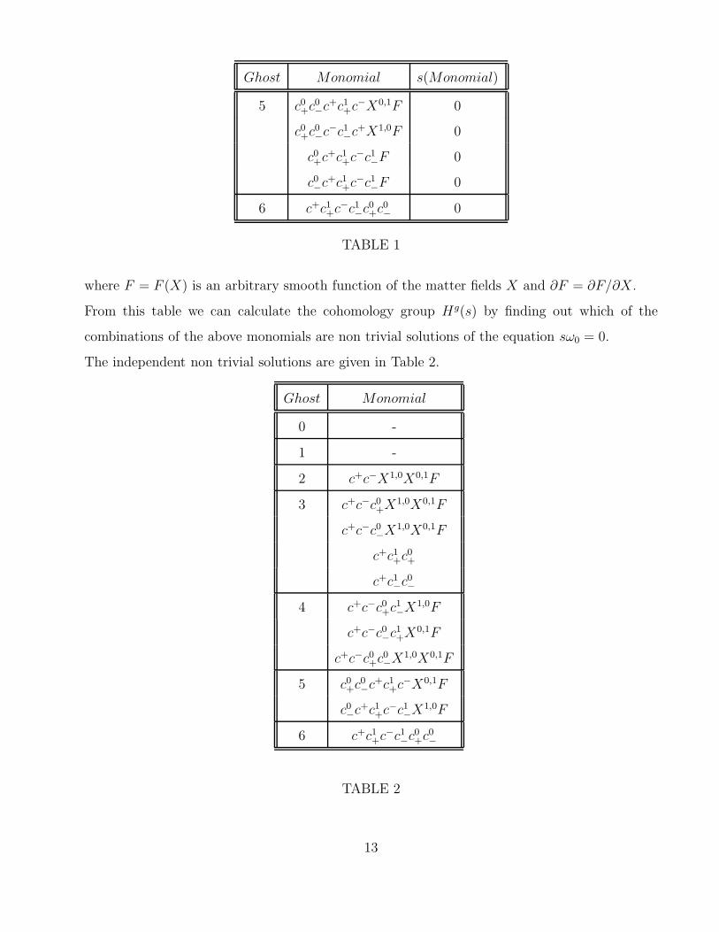
where F = F (X) is an arbitrary smooth function of the matter fields X and ∂F = ∂F/∂X.

From this table we can calculate the cohomology group Hg(s) by finding out which of the

combinations of the above monomials are non trivial solutions of the equation sω0 = 0.

The independent non trivial solutions are given in Table 2.

Ghost Monomial

0 -

1 -

2 c+c−X1,0X0,1F

3 c+c−c0+X1,0X0,1F

c+c−c0−X1,0X0,1F

c+c1+c0+

c+c1−c0−

4 c+c−c0+c1−X

1,0F

c+c−c0−c1+X

0,1F

c+c−c0+c0−X

1,0X0,1F

5 c0+c0−c

+c1+c−X0,1F

c0−c+c1+c

−c1−X1,0F

6 c+c1+c−c1−c

0+c

0−

TABLE 2

13

REMARKS.

1. In the Table 2 we have included only independent solutions of Eq. (3.12) and we have not

given the solutions which differ by those from Table 2 by an s-exact term. For instance for

ghost g = 2 there are two additional solutions of Eq. (3.12) given by

η1 = c+c−c0+X1,1F (4.25)

η2 = c+c−c0−X1,1F (4.26)

but it is easy to verify that they are s-dependent on the ones given in Table 2. Indeed a

little algebra shows that

η1 = c+c−c0+X1,0X0,1∂F + s

[

c+c0+X1,0F

]

and

η2 = c+c−c0+X1,0X0,1∂F + s

[

−c−c0−X0,1F]

.

2. For gh=4 we have only three independent solutions, the rest of five being or s-exact or a

linear combination of these three solutions and some s-exact terms. For instance one can

write

c+c−c0+c0

−X1,1F = −1

2s(c0+c

0

−X1,0F − c−c0+c

0

−X0,1F ) − c+c−c0+c

1

+X1,0F − c+c−c0−c

1

−X0,1F

− c+c−c0+c0

−X1,0X0,1∂F

and

c+c−c0+c1

+X0,1∂F = s(c+c0+c

1

+F ).

3. For gh=5 we have four solutions but only two of them are independent. In this case the

non-independent solutions are

c+c−c0+c1

+c1

−F =1

2s(c+c0+c

0

−c1

+F ) + c+c−c0+c0

−c1

+X0,1F

c+c−c0−c1

+c1

−F =1

2s(c−c0+c

0

−c1

−F ) + c+c−c0+c0

−c1

−X1,0F

14

We must point out that all elements of H(s) given in Table 2 are solutions in the space of

local functions, i.e., in the space of 0-forms. If we want to compute the BRST cohomology in

the space of local functionals ω =∫

d3xf which fulfil the equation sω = 0 we have to solve

the descent equation. As we have been pointing out, these equations can be solved by using the

operator δ defined by

δ = dxα ∂

∂ξα(4.27)

on this way we can write the integrand of ω,ω2 = d2xf in the following form

ω2 =1

2δδω0 (4.28)

and we can compute all terms from the BRST cohomology in the space of local functionals.

The operator δ can be defined directly on the basis used by us as

δc± = dx± + h±±dx∓

dφ = 0 for φ = {h±±, X} (4.29)

and in addition

[δ, ∂±] = 0.

Now it is easy to see that δ is of degree zero and obeys the following relations

d = −[s, δ] [d, δ] = 0. (4.30)

In order to solve the tower (3.10) we shall make use of the following identity

eδs = (s+ d)eδ (4.31)

which is a direct consequence of (4.30) (see [15]). Thanks to this identity we can obtain the

higher cocycles ω1 and ω2 once a non-trivial solution ω0 is known. Indeed, if one apply the

identity (4.31) to ω0 we get

(s+ d)[eδω0] = 0. (4.32)

On the other hand one can see from eq. (4.27) that the operator δ acts as a translation on the

ghosts ξ± with the amount dx± and eq. (4.32) can be rewritten as

(s+ d)ω0(ξ± + dx±, X) = 0. (4.33)

15

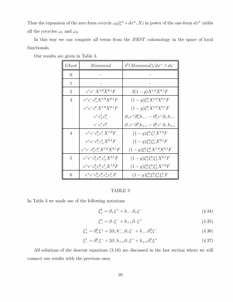
Thus the expansion of the zero form cocycle ω0(ξ±+dx±, X) in power of the one-form dx± yields

all the cocycles ω1 and ω2.

In this way we can compute all terms from the BRST cohomology in the space of local

functionals.

Our results are given in Table 3.

Ghost Monomial δ2(Monomial)/dx+ ∧ dx−

0 - -

1 - -

2 c+c−X1,0X0,1F 2(1 − y)X1,0X0,1F

3 c+c−c0+X1,0X0,1F (1 − y)ξ0

+X1,0X0,1F

c+c−c0−X1,0X0,1F (1 − y)ξ0

−X1,0X0,1F

c+c1+c0+ ∂+c

+∂2+h−− − ∂2

+c+∂+h−−

c−c1−c0− ∂−c

−∂2−h++ − ∂2

−c−∂−h++

4 c+c−c0+c1−X

1,0F (1 − y)ξ0−ξ

1−X

1,0F

c+c−c0−c1+X

0,1F (1 − y)ξ0+ξ

1+X

0,1F

c+c−c0+c0−X

1,0X0,1F (1 − y)ξ0−ξ

0+X

1,0X0,1F

5 c+c−c0+c0−c

1+X

0,1F (1 − y)ξ0+ξ

0−ξ

1+X

0,1F

c+c−c0+c0−c

1−X

1,0F (1 − y)ξ0+ξ

0−ξ

1+X

1,0F

6 c+c−c0+c0−c

1+c

1−F (1 − y)ξ0

+ξ0−ξ

1+ξ

1−F

TABLE 3

In Table 3 we made use of the following notations

ξ0

+ = ∂+ξ+ + h−−∂+ξ

− (4.34)

ξ0

− = ∂−ξ− + h++∂−ξ

+ (4.35)

ξ1

+ = ∂2

+ξ+ + 2∂+h

−−−∂+ξ

− + h−−∂2

+ξ− (4.36)

ξ1

− = ∂2

−ξ− + 2∂−h++∂−ξ

+ + h++∂2

−ξ+ (4.37)

All solutions of the descent equations (3.10) are discussed in the last section where we will

connect our results with the previous ones.

16

5 Discussions and Conclusions

We have determined the complete BRST cohomology group in the space of local fields and

local functionals for a 2D gravitational theory invariant under diffeomorphisms and local Weyl

transformations.

The elements of the BRST group in the space of the local functionals, i.e., the term ω2 in the

descent equations are particularly interesting because they represent classical actions, anomalies

and Schwinger terms. For ghost = 0 there is only one element of H2(s) and it corresponds

to the unique classical action. This action has the form of the σ - model with a torsion term.

For ghost = 1 there are four non-trivial elements of H3(s) which can be grouped in two types.

Representatives of the first type can be chosen to be independent of the matter fields. There are

two independent terms of this type:

∫

d2xc±∂3

±h∓∓ (5.38)

and they represent the candidates for the anomalies [17]. Representatives of the second type

depends nontrivially on the matter fields and have the form:

∫

d2x(1 − y)(∂±ξ± + h±±∂±ξ

∓)(D+X)(D−X) (5.39)

where

ξ± =1

1 − y(c± − h±±c

∓) (5.40)

are the diffeomorphism ghosts. In fact the anomalies of the second type cannot occur in the

perturbative calculations since the classical action S0 does not contain a self-interactive term

in the matter fields. Thus, the numerical coefficient of the corresponding Feynman diagrams

automatically vanishes.

All these solutions have been obtained by Werneck de Oliveira, Schweda and Sorella [12] and

by Brandt, Troost and Van Proeyen [11]. The remarkable point here is the fact that these are

the only possible solutions with ghost number less than two and for the ghost number zero we

have a unique solution.

The solutions of the descent equations (3.10) with ghost number bigger than one do not have

any direct physical significance. Nevertheless we will give all of them for the sake of completeness

17

and for the future use.

For gh=2 we have the following solution of the form:

A2 =∫

d2

[

ξ0

+ξ1

−∇+Xµf 1

µ(X) + ξ0

−ξ1

+∇−Xµf 2

µ(X) +1

1 − yξ0

+ξ0

−∇+Xµ∇−X

νfµν

]

(5.41)

where f 1,2µ (X), fµν(X) are some arbitrary functions of X. In this case the solutions of eqs.(3.10)

depend only on the diffeomorphism ghosts ξ±.

For gh=3 we have also two independent solutions of the form

A3 =∫

d2xξ0

+ξ0

−

[

ξ1

−(∇−Xµf 1

µ(X) + ξ1

−(∇+Xµ)f 2

µ(X)]

. (5.42)

Again in A3 occur only the ghosts ξ±.

In the last possible case gh=4 we have obtained a unique solution of the form

A4 =∫

d2x(1 − y)ξ0

+ξ0

−ξ1

+ξ1

−F (X) (5.43)

with F (X) an arbitrary scalar function of X.

All solutions with ghost number bigger than one are new and as far as we are aware of this

is the first place where they are done.

Finally we want to mention that a similar calculation with the antifields included can be

done [11], but in this case the results strongly depends on the form of the classical action one

starts with.

18

References

[1] C.N. Yang and R.L. Mills, Phys.Rev. 96(1954) 191; S. Glashow and M. Gell-Mann, Ann.

Phys. (N.Y.) 15 (1961) 437;

[2] M.Henneaux and C. Teitelboim, Quantization of Gauge Systems, Princeton University

Press, 1992;

[3] I.A. Batalin and G.A. Vilkovisky, Phys. Rev. D28 (1983) 2567;

[4] G. Barnich, F. Brandt and M. Henneaux, preprint ULB-TH-94/06, NIKEF-H 94-13,

hep/th/9405109

[5] R. Utiyama Phys. Rev. 101 (1956) 1597;

[6] E. Witten, Comm. Math. Phys. 117(1988) 353; Comm. Math. Phys. 118(1988) 411;

[7] R. Stora, Algebraic structure and topological origin of anomalies, Cargese ’83, s. G. t’Hooft

et.al., Plenum Press, New York, 1987;

[8] J. Dixon, Comm. Math. Phys. 139(1991) 495;

[9] J. Wess and B. Zumino, Phys. Lett. B37(1971) 95; B. Zumino, Chiral anomalies and dif-

ferential geometry, Les Houches ’83, eds. B.S. De Witt and R. Stora, North Holland, Ams-

terdam, 1987;

[10] C. Becchi, A. Rouet and R. Stora, Ann. Phys.(N.Y.) 98(1976) 287; I.W. Tyutin Gauge

Invariance in Field Theory and Statistical Physics, Lebedev Institute preprint FIAN

no.39(1975);

[11] F. Brandt, W. Troost and A. Van Proeyen , NIKHEF-H 94-16, KUL-TF-94/17, hep-

th/9407061, to appear in the proceedings of the Geometry of Constrained Dynamical Sys-

tems workshop, Isaac Newton Institute for Mathematical xSciences, Cambridge, June 15-18,

1994; W. Troost and A. Van Proeyen, KUL-TF-94/94, hep-th/9410162;

[12] M. Werneck de Oliveira, M. Schweda and S.P. Sorella, Phys. Lett. B315(1993) 93;

19

[13] F. Brandt, N. Dragon and M. Kreuzer, Nucl. Phys B340(1990) 187;

[14] S.P. Sorella Comm. Math. Phys.157(1993),231;

[15] S.P. Sorella and L. Tataru, Phys. Lett. B324(1994), 351;

[16] A. Boresch, M. Schweda and S.P. Sorella, Phys. Lett. B328(1994);

[17] C. Becchi, Nucl. Phys. B304 513;

[18] L. Baulieu, C. Becchi and R. Stora, Phys. Lett. B180(1986), 55; KUL-TF-94/94, hep-

th/9410162.

[19] L. Baulieu and M. Bellon, Phys. Lett. B196(1987), 142;

[20] R. Grimm Ann. Phys.(N.Y.) 200(1990) 49;

20