2D Geometric Transformations - Cornell CS

© 2006 Steve Marschner • 1Cornell CS465 Fall 2006 •!Lecture 7

2D Geometric Transformations

CS 465 Lecture 7


A little quick math background

• Notation for sets, functions, mappings

• Linear transformations

• Matrices

– Matrix-vector multiplication

– Matrix-matrix multiplication

• Geometry of curves in 2D

– Implicit representation

– Explicit representation


Implicit representations

• Equation to tell whether we are on the curve

• Example: line (orthogonal to u, distance k from 0)

• Example: circle (center p, radius r)

• Always define boundary of region

– (if f is continuous)


Explicit representations

• Also called parametric

• Equation to map domain into plane

• Example: line (containing p, parallel to u)

• Example: circle (center b, radius r)

• Like tracing out the path of a particle over time

• Variable t is the “parameter”


Transforming geometry

• Move a subset of the plane using a mapping from theplane to itself

• Parametric representation:

• Implicit representation:


Translation

• Simplest transformation:

• Inverse:

• Example of transforming circle


Linear transformations

• One way to define a transformation is by matrixmultiplication:

• Such transformations are linear, which is to say:

(and in fact all linear transformations can be written this way)


Geometry of 2D linear trans.

• 2x2 matrices have simple geometric interpretations

– uniform scale

– non-uniform scale

– rotation

– shear

– reflection

• Reading off the matrix


Linear transformation gallery

• Uniform scale



• Nonuniform scale



• Rotation



• Reflection

– can consider it a special caseof nonuniform scale



• Shear


Composing transformations

• Want to move an object, then move it some more

–

• We need to represent S o T (“S compose T”)

– and would like to use the same representation as for S and T

• Translation easy

–

• Translation by uT then by uS is translation by uT + uS

– commutative!


Composing transformations

• Linear transformations also straightforward

–

• Transforming first by MT then by MS is the same astransforming by MSMT

– only sometimes commutative

• e.g. rotations & uniform scales

• e.g. non-uniform scales w/o rotation

– Note MSMT, or S o T, is T first, then S


Combining linear with translation

• Need to use both in single framework

• Can represent arbitrary seq. as

–

–

–

– e. g.

• Transforming by MT and uT, then by MS and uS, is thesame as transforming by MSMT and uS + MSuT

– This will work but is a little awkward


Homogeneous coordinates

• A trick for representing the foregoing more elegantly

• Extra component w for vectors, extra row/column formatrices

– for affine, can always keep w = 1

• Represent linear transformations with dummy extrarow and column



• Represent translation using the extra column



• Composition just works, by 3x3 matrix multiplication

• This is exactly the same as carrying around M and u

– but cleaner

– and generalizes in useful ways as we’ll see later


Affine transformations

• The set of transformations we have been looking at isknown as the “affine” transformations

– straight lines preserved; parallel lines preserved

– ratios of lengths along lines preserved (midpoints preserved)


Affine transformation gallery

• Translation



• Uniform scale



• Nonuniform scale



• Rotation



• Reflection

– can consider it a special caseof nonuniform scale



• Shear


General affine transformations

• The previous slides showed “canonical” examples ofthe types of affine transformations

• Generally, transformations contain elements ofmultiple types

– often define them as products of canonical transforms

– sometimes work with their properties more directly


Composite affine transformations

• In general not commutative: order matters!

rotate, then translate translate, then rotate


Composite affine transformations

• Another example

scale, then rotate rotate, then scale


More math background

• Linear independence and bases

• Orthonormal matrices

• Coordinate systems

– Expressing vectors with respect to bases

– Linear transformations as changes of basis


Rigid motions

• A transform made up of only translation and rotationis a rigid motion or a rigid body transformation

• The linear part is an orthonormal matrix

• Inverse of orthonormal matrix is transpose

– so inverse of rigid motion is easy:


Composing to change axes

• Want to rotate about a particular point

– could work out formulas directly…

• Know how to rotate about the origin

– so translate that point to the origin


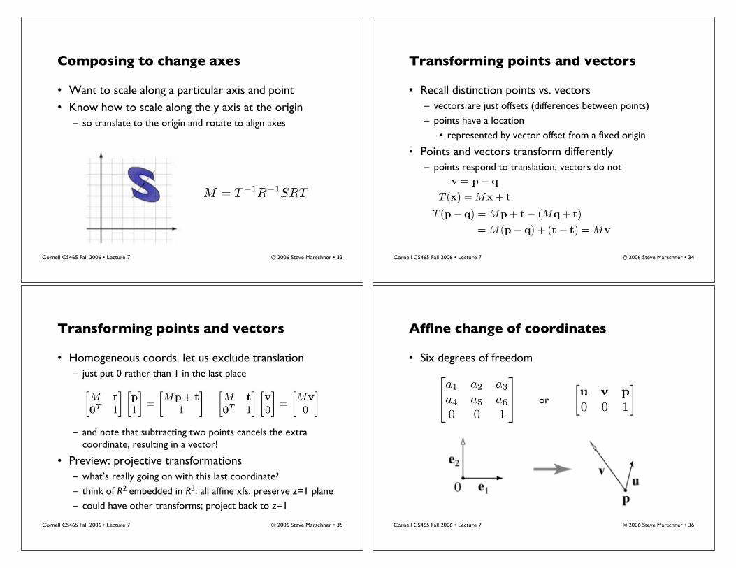
Composing to change axes

• Want to scale along a particular axis and point

• Know how to scale along the y axis at the origin

– so translate to the origin and rotate to align axes


Transforming points and vectors

• Recall distinction points vs. vectors

– vectors are just offsets (differences between points)

– points have a location

• represented by vector offset from a fixed origin

• Points and vectors transform differently

– points respond to translation; vectors do not


Transforming points and vectors

• Homogeneous coords. let us exclude translation

– just put 0 rather than 1 in the last place

– and note that subtracting two points cancels the extracoordinate, resulting in a vector!

• Preview: projective transformations

– what’s really going on with this last coordinate?

– think of R2 embedded in R3: all affine xfs. preserve z=1 plane

– could have other transforms; project back to z=1


Affine change of coordinates

• Six degrees of freedom

or



• Coordinate frame: point plus basis

• Interpretation: transformationchanges representation ofpoint from one basis to another

• “Frame to canonical” matrix hasframe in columns

– takes points represented in frame

– represents them in canonical basis

– e.g. [0 0], [1 0], [0 1]

• Seems backward but bears thinking about



• A new way to “read off” the matrix

– e.g. shear from earlier

– can look at picture, see effecton basis vectors, writedown matrix

• Also an easy way to construct transforms

– e. g. scale by 2 across direction (1,2)



• When we move an object to the origin to apply atransformation, we are really changing coordinates

– the transformation is easy to express in object’s frame

– so define it there and transform it

– Te is the transformation expressed wrt. {e1, e2}

– TF is the transformation expressed in natural frame

– F is the frame-to-canonical matrix [u v p]

• This is a similarity transformation


Coordinate frame summary

• Frame = point plus basis

• Frame matrix (frame-to-canonical) is

• Move points to and from frame by multiplying with F

• Move transformations using similarity transforms

2D Geometric Transformations - Cornell CS

Documents

Transcript of 2D Geometric Transformations - Cornell CS