Foundations of Data Science∗

Avrim Blum, John Hopcroft, and Ravindran Kannan

Monday 21st January, 2019

∗Copyright 2015. All rights reserved

1

Contents

1 Introduction 9

2 High-Dimensional Space 122.1 Introduction . . . . . . . . . . . . . . . . . . . . . . . . . . . . . . . . . . . 122.2 The Law of Large Numbers . . . . . . . . . . . . . . . . . . . . . . . . . . 122.3 The Geometry of High Dimensions . . . . . . . . . . . . . . . . . . . . . . 162.4 Properties of the Unit Ball . . . . . . . . . . . . . . . . . . . . . . . . . . . 17

2.4.1 Volume of the Unit Ball . . . . . . . . . . . . . . . . . . . . . . . . 172.4.2 Volume Near the Equator . . . . . . . . . . . . . . . . . . . . . . . 19

2.5 Generating Points Uniformly at Random from a Ball . . . . . . . . . . . . 222.6 Gaussians in High Dimension . . . . . . . . . . . . . . . . . . . . . . . . . 232.7 Random Projection and Johnson-Lindenstrauss Lemma . . . . . . . . . . . 252.8 Separating Gaussians . . . . . . . . . . . . . . . . . . . . . . . . . . . . . . 272.9 Fitting a Spherical Gaussian to Data . . . . . . . . . . . . . . . . . . . . . 292.10 Bibliographic Notes . . . . . . . . . . . . . . . . . . . . . . . . . . . . . . . 312.11 Exercises . . . . . . . . . . . . . . . . . . . . . . . . . . . . . . . . . . . . . 32

3 Best-Fit Subspaces and Singular Value Decomposition (SVD) 403.1 Introduction . . . . . . . . . . . . . . . . . . . . . . . . . . . . . . . . . . . 403.2 Preliminaries . . . . . . . . . . . . . . . . . . . . . . . . . . . . . . . . . . 423.3 Singular Vectors . . . . . . . . . . . . . . . . . . . . . . . . . . . . . . . . . 433.4 Singular Value Decomposition (SVD) . . . . . . . . . . . . . . . . . . . . . 463.5 Best Rank-k Approximations . . . . . . . . . . . . . . . . . . . . . . . . . 473.6 Left Singular Vectors . . . . . . . . . . . . . . . . . . . . . . . . . . . . . . 493.7 Power Method for Singular Value Decomposition . . . . . . . . . . . . . . . 51

3.7.1 A Faster Method . . . . . . . . . . . . . . . . . . . . . . . . . . . . 523.8 Singular Vectors and Eigenvectors . . . . . . . . . . . . . . . . . . . . . . . 543.9 Applications of Singular Value Decomposition . . . . . . . . . . . . . . . . 54

3.9.1 Centering Data . . . . . . . . . . . . . . . . . . . . . . . . . . . . . 543.9.2 Principal Component Analysis . . . . . . . . . . . . . . . . . . . . . 563.9.3 Clustering a Mixture of Spherical Gaussians . . . . . . . . . . . . . 573.9.4 Ranking Documents and Web Pages . . . . . . . . . . . . . . . . . 623.9.5 An Illustrative Application of SVD . . . . . . . . . . . . . . . . . . 633.9.6 An Application of SVD to a Discrete Optimization Problem . . . . 64

3.10 Bibliographic Notes . . . . . . . . . . . . . . . . . . . . . . . . . . . . . . . 663.11 Exercises . . . . . . . . . . . . . . . . . . . . . . . . . . . . . . . . . . . . . 68

4 Random Walks and Markov Chains 774.1 Stationary Distribution . . . . . . . . . . . . . . . . . . . . . . . . . . . . . 814.2 Markov Chain Monte Carlo . . . . . . . . . . . . . . . . . . . . . . . . . . 82

4.2.1 Metropolis-Hasting Algorithm . . . . . . . . . . . . . . . . . . . . . 844.2.2 Gibbs Sampling . . . . . . . . . . . . . . . . . . . . . . . . . . . . . 85

2

4.3 Areas and Volumes . . . . . . . . . . . . . . . . . . . . . . . . . . . . . . . 874.4 Convergence of Random Walks on Undirected Graphs . . . . . . . . . . . . 89

4.4.1 Using Normalized Conductance to Prove Convergence . . . . . . . . 954.5 Electrical Networks and Random Walks . . . . . . . . . . . . . . . . . . . . 984.6 Random Walks on Undirected Graphs with Unit Edge Weights . . . . . . . 1034.7 Random Walks in Euclidean Space . . . . . . . . . . . . . . . . . . . . . . 1104.8 The Web as a Markov Chain . . . . . . . . . . . . . . . . . . . . . . . . . . 1134.9 Bibliographic Notes . . . . . . . . . . . . . . . . . . . . . . . . . . . . . . . 1174.10 Exercises . . . . . . . . . . . . . . . . . . . . . . . . . . . . . . . . . . . . . 119

5 Machine Learning 1325.1 Introduction . . . . . . . . . . . . . . . . . . . . . . . . . . . . . . . . . . . 1325.2 The Perceptron Algorithm . . . . . . . . . . . . . . . . . . . . . . . . . . . 1335.3 Kernel Functions and Non-linearly Separable Data . . . . . . . . . . . . . . 1355.4 Generalizing to New Data . . . . . . . . . . . . . . . . . . . . . . . . . . . 136

5.4.1 Overfitting and Uniform Convergence . . . . . . . . . . . . . . . . . 1385.4.2 Occam’s Razor . . . . . . . . . . . . . . . . . . . . . . . . . . . . . 1405.4.3 Regularization: Penalizing Complexity . . . . . . . . . . . . . . . . 141

5.5 VC-Dimension . . . . . . . . . . . . . . . . . . . . . . . . . . . . . . . . . . 1425.5.1 Definitions and Key Theorems . . . . . . . . . . . . . . . . . . . . . 1435.5.2 VC-Dimension of Some Set Systems . . . . . . . . . . . . . . . . . 1445.5.3 Shatter Function for Set Systems of Bounded VC-Dimension . . . 1465.5.4 VC-Dimension of Combinations of Concepts . . . . . . . . . . . . . 1485.5.5 The Key Theorem . . . . . . . . . . . . . . . . . . . . . . . . . . . 149

5.6 VC-dimension and Machine Learning . . . . . . . . . . . . . . . . . . . . . 1505.7 Other Measures of Complexity . . . . . . . . . . . . . . . . . . . . . . . . . 1515.8 Deep Learning . . . . . . . . . . . . . . . . . . . . . . . . . . . . . . . . . . 152

5.8.1 Generative Adversarial Networks (GANs) . . . . . . . . . . . . . . . 1585.9 Gradient Descent . . . . . . . . . . . . . . . . . . . . . . . . . . . . . . . . 159

5.9.1 Stochastic Gradient Descent . . . . . . . . . . . . . . . . . . . . . . 1615.9.2 Regularizer . . . . . . . . . . . . . . . . . . . . . . . . . . . . . . . 163

5.10 Online Learning . . . . . . . . . . . . . . . . . . . . . . . . . . . . . . . . . 1635.10.1 An Example: Learning Disjunctions . . . . . . . . . . . . . . . . . . 1645.10.2 The Halving Algorithm . . . . . . . . . . . . . . . . . . . . . . . . . 1655.10.3 The Perceptron Algorithm . . . . . . . . . . . . . . . . . . . . . . . 1655.10.4 Inseparable Data and Hinge Loss . . . . . . . . . . . . . . . . . . . 1665.10.5 Online to Batch Conversion . . . . . . . . . . . . . . . . . . . . . . 1675.10.6 Combining (Sleeping) Expert Advice . . . . . . . . . . . . . . . . . 168

5.11 Boosting . . . . . . . . . . . . . . . . . . . . . . . . . . . . . . . . . . . . . 1715.12 Further Current Directions . . . . . . . . . . . . . . . . . . . . . . . . . . . 174

5.12.1 Semi-Supervised Learning . . . . . . . . . . . . . . . . . . . . . . . 1745.12.2 Active Learning . . . . . . . . . . . . . . . . . . . . . . . . . . . . . 1765.12.3 Multi-Task Learning . . . . . . . . . . . . . . . . . . . . . . . . . . 177

3

5.13 Bibliographic Notes . . . . . . . . . . . . . . . . . . . . . . . . . . . . . . . 1785.14 Exercises . . . . . . . . . . . . . . . . . . . . . . . . . . . . . . . . . . . . . 179

6 Algorithms for Massive Data Problems: Streaming, Sketching, andSampling 1856.1 Introduction . . . . . . . . . . . . . . . . . . . . . . . . . . . . . . . . . . . 1856.2 Frequency Moments of Data Streams . . . . . . . . . . . . . . . . . . . . . 186

6.2.1 Number of Distinct Elements in a Data Stream . . . . . . . . . . . 1876.2.2 Number of Occurrences of a Given Element. . . . . . . . . . . . . . 1906.2.3 Frequent Elements . . . . . . . . . . . . . . . . . . . . . . . . . . . 1916.2.4 The Second Moment . . . . . . . . . . . . . . . . . . . . . . . . . . 193

6.3 Matrix Algorithms using Sampling . . . . . . . . . . . . . . . . . . . . . . 1966.3.1 Matrix Multiplication using Sampling . . . . . . . . . . . . . . . . . 1976.3.2 Implementing Length Squared Sampling in Two Passes . . . . . . . 2006.3.3 Sketch of a Large Matrix . . . . . . . . . . . . . . . . . . . . . . . . 201

6.4 Sketches of Documents . . . . . . . . . . . . . . . . . . . . . . . . . . . . . 2056.5 Bibliographic Notes . . . . . . . . . . . . . . . . . . . . . . . . . . . . . . . 2076.6 Exercises . . . . . . . . . . . . . . . . . . . . . . . . . . . . . . . . . . . . . 208

7 Clustering 2127.1 Introduction . . . . . . . . . . . . . . . . . . . . . . . . . . . . . . . . . . . 212

7.1.1 Preliminaries . . . . . . . . . . . . . . . . . . . . . . . . . . . . . . 2127.1.2 Two General Assumptions on the Form of Clusters . . . . . . . . . 2137.1.3 Spectral Clustering . . . . . . . . . . . . . . . . . . . . . . . . . . . 215

7.2 k-Means Clustering . . . . . . . . . . . . . . . . . . . . . . . . . . . . . . . 2157.2.1 A Maximum-Likelihood Motivation . . . . . . . . . . . . . . . . . . 2157.2.2 Structural Properties of the k-Means Objective . . . . . . . . . . . 2167.2.3 Lloyd’s Algorithm . . . . . . . . . . . . . . . . . . . . . . . . . . . . 2177.2.4 Ward’s Algorithm . . . . . . . . . . . . . . . . . . . . . . . . . . . . 2197.2.5 k-Means Clustering on the Line . . . . . . . . . . . . . . . . . . . . 219

7.3 k-Center Clustering . . . . . . . . . . . . . . . . . . . . . . . . . . . . . . . 2197.4 Finding Low-Error Clusterings . . . . . . . . . . . . . . . . . . . . . . . . . 2207.5 Spectral Clustering . . . . . . . . . . . . . . . . . . . . . . . . . . . . . . . 220

7.5.1 Why Project? . . . . . . . . . . . . . . . . . . . . . . . . . . . . . . 2207.5.2 The Algorithm . . . . . . . . . . . . . . . . . . . . . . . . . . . . . 2227.5.3 Means Separated by Ω(1) Standard Deviations . . . . . . . . . . . . 2237.5.4 Laplacians . . . . . . . . . . . . . . . . . . . . . . . . . . . . . . . . 2257.5.5 Local spectral clustering . . . . . . . . . . . . . . . . . . . . . . . . 225

7.6 Approximation Stability . . . . . . . . . . . . . . . . . . . . . . . . . . . . 2287.6.1 The Conceptual Idea . . . . . . . . . . . . . . . . . . . . . . . . . . 2287.6.2 Making this Formal . . . . . . . . . . . . . . . . . . . . . . . . . . . 2287.6.3 Algorithm and Analysis . . . . . . . . . . . . . . . . . . . . . . . . 229

7.7 High-Density Clusters . . . . . . . . . . . . . . . . . . . . . . . . . . . . . 231

4

7.7.1 Single Linkage . . . . . . . . . . . . . . . . . . . . . . . . . . . . . . 2317.7.2 Robust Linkage . . . . . . . . . . . . . . . . . . . . . . . . . . . . . 232

7.8 Kernel Methods . . . . . . . . . . . . . . . . . . . . . . . . . . . . . . . . . 2327.9 Recursive Clustering Based on Sparse Cuts . . . . . . . . . . . . . . . . . . 2337.10 Dense Submatrices and Communities . . . . . . . . . . . . . . . . . . . . . 2347.11 Community Finding and Graph Partitioning . . . . . . . . . . . . . . . . . 2377.12 Spectral Clustering Applied to Social Networks . . . . . . . . . . . . . . . 2407.13 Bibliographic Notes . . . . . . . . . . . . . . . . . . . . . . . . . . . . . . . 2437.14 Exercises . . . . . . . . . . . . . . . . . . . . . . . . . . . . . . . . . . . . . 244

8 Random Graphs 2498.1 The G(n, p) Model . . . . . . . . . . . . . . . . . . . . . . . . . . . . . . . 249

8.1.1 Degree Distribution . . . . . . . . . . . . . . . . . . . . . . . . . . . 2508.1.2 Existence of Triangles in G(n, d/n) . . . . . . . . . . . . . . . . . . 254

8.2 Phase Transitions . . . . . . . . . . . . . . . . . . . . . . . . . . . . . . . . 2568.3 Giant Component . . . . . . . . . . . . . . . . . . . . . . . . . . . . . . . . 268

8.3.1 Existence of a Giant Component . . . . . . . . . . . . . . . . . . . 2688.3.2 No Other Large Components . . . . . . . . . . . . . . . . . . . . . 2708.3.3 The Case of p < 1/n . . . . . . . . . . . . . . . . . . . . . . . . . . 270

8.4 Cycles and Full Connectivity . . . . . . . . . . . . . . . . . . . . . . . . . . 2718.4.1 Emergence of Cycles . . . . . . . . . . . . . . . . . . . . . . . . . . 2718.4.2 Full Connectivity . . . . . . . . . . . . . . . . . . . . . . . . . . . . 2728.4.3 Threshold for O(lnn) Diameter . . . . . . . . . . . . . . . . . . . . 274

8.5 Phase Transitions for Increasing Properties . . . . . . . . . . . . . . . . . . 2768.6 Branching Processes . . . . . . . . . . . . . . . . . . . . . . . . . . . . . . 2788.7 CNF-SAT . . . . . . . . . . . . . . . . . . . . . . . . . . . . . . . . . . . . 284

8.7.1 SAT-solvers in practice . . . . . . . . . . . . . . . . . . . . . . . . . 2848.7.2 Phase Transitions for CNF-SAT . . . . . . . . . . . . . . . . . . . . 285

8.8 Non-uniform Models of Random Graphs . . . . . . . . . . . . . . . . . . . 2908.8.1 Giant Component in Graphs with Given Degree Distribution . . . . 291

8.9 Growth Models . . . . . . . . . . . . . . . . . . . . . . . . . . . . . . . . . 2928.9.1 Growth Model Without Preferential Attachment . . . . . . . . . . . 2938.9.2 Growth Model With Preferential Attachment . . . . . . . . . . . . 299

8.10 Small World Graphs . . . . . . . . . . . . . . . . . . . . . . . . . . . . . . 3008.11 Bibliographic Notes . . . . . . . . . . . . . . . . . . . . . . . . . . . . . . . 3068.12 Exercises . . . . . . . . . . . . . . . . . . . . . . . . . . . . . . . . . . . . . 307

9 Topic Models, Non-negative Matrix Factorization, Hidden Markov Mod-els, and Graphical Models 3169.1 Topic Models . . . . . . . . . . . . . . . . . . . . . . . . . . . . . . . . . . 3169.2 An Idealized Model . . . . . . . . . . . . . . . . . . . . . . . . . . . . . . . 3199.3 Non-negative Matrix Factorization - NMF . . . . . . . . . . . . . . . . . . 3219.4 NMF with Anchor Terms . . . . . . . . . . . . . . . . . . . . . . . . . . . . 323

5

9.5 Hard and Soft Clustering . . . . . . . . . . . . . . . . . . . . . . . . . . . . 3249.6 The Latent Dirichlet Allocation Model for Topic Modeling . . . . . . . . . 3269.7 The Dominant Admixture Model . . . . . . . . . . . . . . . . . . . . . . . 3289.8 Formal Assumptions . . . . . . . . . . . . . . . . . . . . . . . . . . . . . . 3309.9 Finding the Term-Topic Matrix . . . . . . . . . . . . . . . . . . . . . . . . 3339.10 Hidden Markov Models . . . . . . . . . . . . . . . . . . . . . . . . . . . . . 3389.11 Graphical Models and Belief Propagation . . . . . . . . . . . . . . . . . . . 3439.12 Bayesian or Belief Networks . . . . . . . . . . . . . . . . . . . . . . . . . . 3449.13 Markov Random Fields . . . . . . . . . . . . . . . . . . . . . . . . . . . . . 3459.14 Factor Graphs . . . . . . . . . . . . . . . . . . . . . . . . . . . . . . . . . . 3469.15 Tree Algorithms . . . . . . . . . . . . . . . . . . . . . . . . . . . . . . . . . 3479.16 Message Passing in General Graphs . . . . . . . . . . . . . . . . . . . . . . 348

9.16.1 Graphs with a Single Cycle . . . . . . . . . . . . . . . . . . . . . . 3509.16.2 Belief Update in Networks with a Single Loop . . . . . . . . . . . . 3529.16.3 Maximum Weight Matching . . . . . . . . . . . . . . . . . . . . . . 353

9.17 Warning Propagation . . . . . . . . . . . . . . . . . . . . . . . . . . . . . . 3579.18 Correlation Between Variables . . . . . . . . . . . . . . . . . . . . . . . . . 3579.19 Bibliographic Notes . . . . . . . . . . . . . . . . . . . . . . . . . . . . . . . 3619.20 Exercises . . . . . . . . . . . . . . . . . . . . . . . . . . . . . . . . . . . . . 363

10 Other Topics 36610.1 Ranking and Social Choice . . . . . . . . . . . . . . . . . . . . . . . . . . . 366

10.1.1 Randomization . . . . . . . . . . . . . . . . . . . . . . . . . . . . . 36810.1.2 Examples . . . . . . . . . . . . . . . . . . . . . . . . . . . . . . . . 369

10.2 Compressed Sensing and Sparse Vectors . . . . . . . . . . . . . . . . . . . 37010.2.1 Unique Reconstruction of a Sparse Vector . . . . . . . . . . . . . . 37110.2.2 Efficiently Finding the Unique Sparse Solution . . . . . . . . . . . . 372

10.3 Applications . . . . . . . . . . . . . . . . . . . . . . . . . . . . . . . . . . . 37410.3.1 Biological . . . . . . . . . . . . . . . . . . . . . . . . . . . . . . . . 37410.3.2 Low Rank Matrices . . . . . . . . . . . . . . . . . . . . . . . . . . . 375

10.4 An Uncertainty Principle . . . . . . . . . . . . . . . . . . . . . . . . . . . . 37610.4.1 Sparse Vector in Some Coordinate Basis . . . . . . . . . . . . . . . 37610.4.2 A Representation Cannot be Sparse in Both Time and Frequency

Domains . . . . . . . . . . . . . . . . . . . . . . . . . . . . . . . . . 37710.5 Gradient . . . . . . . . . . . . . . . . . . . . . . . . . . . . . . . . . . . . . 37910.6 Linear Programming . . . . . . . . . . . . . . . . . . . . . . . . . . . . . . 381

10.6.1 The Ellipsoid Algorithm . . . . . . . . . . . . . . . . . . . . . . . . 38110.7 Integer Optimization . . . . . . . . . . . . . . . . . . . . . . . . . . . . . . 38310.8 Semi-Definite Programming . . . . . . . . . . . . . . . . . . . . . . . . . . 38410.9 Bibliographic Notes . . . . . . . . . . . . . . . . . . . . . . . . . . . . . . . 38610.10Exercises . . . . . . . . . . . . . . . . . . . . . . . . . . . . . . . . . . . . . 387

6

11 Wavelets 39111.1 Dilation . . . . . . . . . . . . . . . . . . . . . . . . . . . . . . . . . . . . . 39111.2 The Haar Wavelet . . . . . . . . . . . . . . . . . . . . . . . . . . . . . . . . 39211.3 Wavelet Systems . . . . . . . . . . . . . . . . . . . . . . . . . . . . . . . . 39611.4 Solving the Dilation Equation . . . . . . . . . . . . . . . . . . . . . . . . . 39611.5 Conditions on the Dilation Equation . . . . . . . . . . . . . . . . . . . . . 39811.6 Derivation of the Wavelets from the Scaling Function . . . . . . . . . . . . 40011.7 Sufficient Conditions for the Wavelets to be Orthogonal . . . . . . . . . . . 40411.8 Expressing a Function in Terms of Wavelets . . . . . . . . . . . . . . . . . 40711.9 Designing a Wavelet System . . . . . . . . . . . . . . . . . . . . . . . . . . 40711.10Applications . . . . . . . . . . . . . . . . . . . . . . . . . . . . . . . . . . . 40811.11 Bibliographic Notes . . . . . . . . . . . . . . . . . . . . . . . . . . . . . . 40811.12 Exercises . . . . . . . . . . . . . . . . . . . . . . . . . . . . . . . . . . . . 409

12 Appendix 41212.1 Definitions and Notation . . . . . . . . . . . . . . . . . . . . . . . . . . . . 412

12.1.1 Integers . . . . . . . . . . . . . . . . . . . . . . . . . . . . . . . . . 41212.1.2 Substructures . . . . . . . . . . . . . . . . . . . . . . . . . . . . . . 41212.1.3 Asymptotic Notation . . . . . . . . . . . . . . . . . . . . . . . . . . 412

12.2 Useful Relations . . . . . . . . . . . . . . . . . . . . . . . . . . . . . . . . . 41412.3 Useful Inequalities . . . . . . . . . . . . . . . . . . . . . . . . . . . . . . . 41812.4 Probability . . . . . . . . . . . . . . . . . . . . . . . . . . . . . . . . . . . 425

12.4.1 Sample Space, Events, and Independence . . . . . . . . . . . . . . . 42612.4.2 Linearity of Expectation . . . . . . . . . . . . . . . . . . . . . . . . 42712.4.3 Union Bound . . . . . . . . . . . . . . . . . . . . . . . . . . . . . . 42712.4.4 Indicator Variables . . . . . . . . . . . . . . . . . . . . . . . . . . . 42712.4.5 Variance . . . . . . . . . . . . . . . . . . . . . . . . . . . . . . . . . 42812.4.6 Variance of the Sum of Independent Random Variables . . . . . . . 42812.4.7 Median . . . . . . . . . . . . . . . . . . . . . . . . . . . . . . . . . 42812.4.8 The Central Limit Theorem . . . . . . . . . . . . . . . . . . . . . . 42912.4.9 Probability Distributions . . . . . . . . . . . . . . . . . . . . . . . . 42912.4.10 Bayes Rule and Estimators . . . . . . . . . . . . . . . . . . . . . . . 433

12.5 Bounds on Tail Probability . . . . . . . . . . . . . . . . . . . . . . . . . . . 43512.5.1 Chernoff Bounds . . . . . . . . . . . . . . . . . . . . . . . . . . . . 43512.5.2 More General Tail Bounds . . . . . . . . . . . . . . . . . . . . . . . 438

12.6 Applications of the Tail Bound . . . . . . . . . . . . . . . . . . . . . . . . 44112.7 Eigenvalues and Eigenvectors . . . . . . . . . . . . . . . . . . . . . . . . . 443

12.7.1 Symmetric Matrices . . . . . . . . . . . . . . . . . . . . . . . . . . 44412.7.2 Relationship between SVD and Eigen Decomposition . . . . . . . . 44612.7.3 Extremal Properties of Eigenvalues . . . . . . . . . . . . . . . . . . 44712.7.4 Eigenvalues of the Sum of Two Symmetric Matrices . . . . . . . . . 44912.7.5 Norms . . . . . . . . . . . . . . . . . . . . . . . . . . . . . . . . . . 45012.7.6 Important Norms and Their Properties . . . . . . . . . . . . . . . . 451

7

12.7.7 Additional Linear Algebra . . . . . . . . . . . . . . . . . . . . . . . 45312.7.8 Distance Between Subspaces . . . . . . . . . . . . . . . . . . . . . . 45512.7.9 Positive Semidefinite Matrix . . . . . . . . . . . . . . . . . . . . . . 456

12.8 Generating Functions . . . . . . . . . . . . . . . . . . . . . . . . . . . . . 45612.8.1 Generating Functions for Sequences Defined by Recurrence Rela-

tionships . . . . . . . . . . . . . . . . . . . . . . . . . . . . . . . . . 45712.8.2 The Exponential Generating Function and the Moment Generating

Function . . . . . . . . . . . . . . . . . . . . . . . . . . . . . . . . . 45912.9 Miscellaneous . . . . . . . . . . . . . . . . . . . . . . . . . . . . . . . . . . 461

12.9.1 Lagrange Multipliers . . . . . . . . . . . . . . . . . . . . . . . . . . 46112.9.2 Finite Fields . . . . . . . . . . . . . . . . . . . . . . . . . . . . . . . 46212.9.3 Application of Mean Value Theorem . . . . . . . . . . . . . . . . . 462

12.10Exercises . . . . . . . . . . . . . . . . . . . . . . . . . . . . . . . . . . . . . 464

Index 469

8

1 Introduction

Computer science as an academic discipline began in the 1960’s. Emphasis was onprogramming languages, compilers, operating systems, and the mathematical theory thatsupported these areas. Courses in theoretical computer science covered finite automata,regular expressions, context-free languages, and computability. In the 1970’s, the studyof algorithms was added as an important component of theory. The emphasis was onmaking computers useful. Today, a fundamental change is taking place and the focus ismore on a wealth of applications. There are many reasons for this change. The mergingof computing and communications has played an important role. The enhanced abilityto observe, collect, and store data in the natural sciences, in commerce, and in otherfields calls for a change in our understanding of data and how to handle it in the modernsetting. The emergence of the web and social networks as central aspects of daily lifepresents both opportunities and challenges for theory.

While traditional areas of computer science remain highly important, increasingly re-searchers of the future will be involved with using computers to understand and extractusable information from massive data arising in applications, not just how to make com-puters useful on specific well-defined problems. With this in mind we have written thisbook to cover the theory we expect to be useful in the next 40 years, just as an under-standing of automata theory, algorithms, and related topics gave students an advantagein the last 40 years. One of the major changes is an increase in emphasis on probability,statistics, and numerical methods.

Early drafts of the book have been used for both undergraduate and graduate courses.Background material needed for an undergraduate course has been put in the appendix.For this reason, the appendix has homework problems.

Modern data in diverse fields such as information processing, search, and machinelearning is often advantageously represented as vectors with a large number of compo-nents. The vector representation is not just a book-keeping device to store many fieldsof a record. Indeed, the two salient aspects of vectors: geometric (length, dot products,orthogonality, etc.) and linear algebraic (independence, rank, singular values, etc.) turnout to be relevant and useful. Chapters 2 and 3 lay the foundations of geometry andlinear algebra respectively. More specifically, our intuition from two or three dimensionalspace can be surprisingly off the mark when it comes to high dimensions. Chapter 2works out the fundamentals needed to understand the differences. The emphasis of thechapter, as well as the book in general, is to get across the intellectual ideas and themathematical foundations rather than focus on particular applications, some of which arebriefly described. Chapter 3 focuses on singular value decomposition (SVD) a central toolto deal with matrix data. We give a from-first-principles description of the mathematicsand algorithms for SVD. Applications of singular value decomposition include principalcomponent analysis, a widely used technique which we touch upon, as well as modern

9

applications to statistical mixtures of probability densities, discrete optimization, etc.,which are described in more detail.

Exploring large structures like the web or the space of configurations of a large systemwith deterministic methods can be prohibitively expensive. Random walks (also calledMarkov Chains) turn out often to be more efficient as well as illuminative. The station-ary distributions of such walks are important for applications ranging from web search tothe simulation of physical systems. The underlying mathematical theory of such randomwalks, as well as connections to electrical networks, forms the core of Chapter 4 on Markovchains.

One of the surprises of computer science over the last two decades is that some domain-independent methods have been immensely successful in tackling problems from diverseareas. Machine learning is a striking example. Chapter 5 describes the foundationsof machine learning, both algorithms for optimizing over given training examples, aswell as the theory for understanding when such optimization can be expected to lead togood performance on new, unseen data. This includes important measures such as theVapnik-Chervonenkis dimension, important algorithms such as the Perceptron Algorithm,stochastic gradient descent, boosting, and deep learning, and important notions such asregularization and overfitting.

The field of algorithms has traditionally assumed that the input data to a problem ispresented in random access memory, which the algorithm can repeatedly access. This isnot feasible for problems involving enormous amounts of data. The streaming model andother models have been formulated to reflect this. In this setting, sampling plays a crucialrole and, indeed, we have to sample on the fly. In Chapter 6 we study how to draw goodsamples efficiently and how to estimate statistical and linear algebra quantities, with suchsamples.

While Chapter 5 focuses on supervised learning, where one learns from labeled trainingdata, the problem of unsupervised learning, or learning from unlabeled data, is equallyimportant. A central topic in unsupervised learning is clustering, discussed in Chapter7. Clustering refers to the problem of partitioning data into groups of similar objects.After describing some of the basic methods for clustering, such as the k-means algorithm,Chapter 7 focuses on modern developments in understanding these, as well as newer al-gorithms and general frameworks for analyzing different kinds of clustering problems.

Central to our understanding of large structures, like the web and social networks, isbuilding models to capture essential properties of these structures. The simplest modelis that of a random graph formulated by Erdos and Renyi, which we study in detail inChapter 8, proving that certain global phenomena, like a giant connected component,arise in such structures with only local choices. We also describe other models of randomgraphs.

10

Chapter 9 focuses on linear-algebraic problems of making sense from data, in par-ticular topic modeling and non-negative matrix factorization. In addition to discussingwell-known models, we also describe some current research on models and algorithms withprovable guarantees on learning error and time. This is followed by graphical models andbelief propagation.

Chapter 10 discusses ranking and social choice as well as problems of sparse represen-tations such as compressed sensing. Additionally, Chapter 10 includes a brief discussionof linear programming and semidefinite programming. Wavelets, which are an impor-tant method for representing signals across a wide range of applications, are discussed inChapter 11 along with some of their fundamental mathematical properties. The appendixincludes a range of background material.

A word about notation in the book. To help the student, we have adopted certainnotations, and with a few exceptions, adhered to them. We use lower case letters forscalar variables and functions, bold face lower case for vectors, and upper case lettersfor matrices. Lower case near the beginning of the alphabet tend to be constants, in themiddle of the alphabet, such as i, j, and k, are indices in summations, n and m for integersizes, and x, y and z for variables. If A is a matrix its elements are aij and its rows are ai.If ai is a vector its coordinates are aij. Where the literature traditionally uses a symbolfor a quantity, we also used that symbol, even if it meant abandoning our convention. Ifwe have a set of points in some vector space, and work with a subspace, we use n for thenumber of points, d for the dimension of the space, and k for the dimension of the subspace.

The term “almost surely” means with probability tending to one. We use lnn for thenatural logarithm and log n for the base two logarithm. If we want base ten, we will use

log10 . To simplify notation and to make it easier to read we use E2(1−x) for(E(1− x)

)2

and E(1− x)2 for E((1− x)2

). When we say “randomly select” some number of points

from a given probability distribution, independence is always assumed unless otherwisestated.

11

2 High-Dimensional Space

2.1 Introduction

High dimensional data has become very important. However, high dimensional spaceis very different from the two and three dimensional spaces we are familiar with. Generaten points at random in d-dimensions where each coordinate is a zero mean, unit varianceGaussian. For sufficiently large d, with high probability the distances between all pairsof points will be essentially the same. Also the volume of the unit ball in d-dimensions,the set of all points x such that |x| ≤ 1, goes to zero as the dimension goes to infinity.The volume of a high dimensional unit ball is concentrated near its surface and is alsoconcentrated at its equator. These properties have important consequences which we willconsider.

2.2 The Law of Large Numbers

If one generates random points in d-dimensional space using a Gaussian to generatecoordinates, the distance between all pairs of points will be essentially the same when dis large. The reason is that the square of the distance between two points y and z,

|y − z|2 =d∑i=1

(yi − zi)2,

can be viewed as the sum of d independent samples of a random variable x that is thesquared difference of two Gaussians. In particular, we are summing independent samplesxi = (yi−zi)2 of a random variable x of bounded variance. In such a case, a general boundknown as the Law of Large Numbers states that with high probability, the average of thesamples will be close to the expectation of the random variable. This in turn implies thatwith high probability, the sum is close to the sum’s expectation.

Specifically, the Law of Large Numbers states that

Prob

(∣∣∣∣x1 + x2 + · · ·+ xnn

− E(x)

∣∣∣∣ ≥ ε

)≤ V ar(x)

nε2. (2.1)

The larger the variance of the random variable, the greater the probability that the errorwill exceed ε. Thus the variance of x is in the numerator. The number of samples n is inthe denominator since the more values that are averaged, the smaller the probability thatthe difference will exceed ε. Similarly the larger ε is, the smaller the probability that thedifference will exceed ε and hence ε is in the denominator. Notice that squaring ε makesthe fraction a dimensionless quantity.

We use two inequalities to prove the Law of Large Numbers. The first is Markov’sinequality that states that the probability that a non-negative random variable exceeds ais bounded by the expected value of the variable divided by a.

12

Theorem 2.1 (Markov’s inequality) Let x be a non-negative random variable. Thenfor a > 0,

Prob(x ≥ a) ≤ E(x)

a.

Proof: For a continuous non-negative random variable x with probability density p,

E (x) =

∞∫0

xp(x)dx =

a∫0

xp(x)dx+

∞∫a

xp(x)dx

≥∞∫a

xp(x)dx ≥ a

∞∫a

p(x)dx = aProb(x ≥ a).

Thus, Prob(x ≥ a) ≤ E(x)a.

The same proof works for discrete random variables with sums instead of integrals.

Corollary 2.2 Prob(x ≥ bE(x)

)≤ 1

b

Markov’s inequality bounds the tail of a distribution using only information about themean. A tighter bound can be obtained by also using the variance of the random variable.

Theorem 2.3 (Chebyshev’s inequality) Let x be a random variable. Then for c > 0,

Prob(|x− E(x)| ≥ c

)≤ V ar(x)

c2.

Proof: Prob(|x− E(x)| ≥ c

)= Prob

(|x− E(x)|2 ≥ c2

). Note that y = |x− E(x)|2 is a

non-negative random variable and E(y) = V ar(x), so Markov’s inequality can be appliedgiving:

Prob(|x− E(x)| ≥ c) = Prob(|x− E(x)|2 ≥ c2

)≤ E(|x− E(x)|2)

c2=V ar(x)

c2.

The Law of Large Numbers follows from Chebyshev’s inequality together with factsabout independent random variables. Recall that:

E(x+ y) = E(x) + E(y),

V ar(x− c) = V ar(x),

V ar(cx) = c2V ar(x).

13

Also, if x and y are independent, then E(xy) = E(x)E(y). These facts imply that if xand y are independent then V ar(x+ y) = V ar(x) + V ar(y), which is seen as follows:

V ar(x+ y) = E(x+ y)2 − E2(x+ y)

= E(x2 + 2xy + y2)−(E2(x) + 2E(x)E(y) + E2(y)

)= E(x2)− E2(x) + E(y2)− E2(y) = V ar(x) + V ar(y),

where we used independence to replace E(2xy) with 2E(x)E(y).

Theorem 2.4 (Law of Large Numbers) Let x1, x2, . . . , xn be n independent samplesof a random variable x. Then

Prob(∣∣∣x1 + x2 + · · ·+ xn

n− E(x)

∣∣∣ ≥ ε)≤ V ar(x)

nε2

Proof: E(x1+x2+···+xn

n

)= E(x) and thus

Prob(∣∣∣x1 + x2 + · · ·+ xn

n−E(x)

∣∣∣ ≥ ε)

= Prob(∣∣∣x1 + x2 + · · ·+ xn

n−E(x1 + x2 + · · ·+ xn

n

)∣∣∣ ≥ ε)

By Chebyshev’s inequality

Prob(∣∣∣x1 + x2 + · · ·+ xn

n− E(x)

∣∣∣ ≥ ε)

= Prob(∣∣∣x1 + x2 + · · ·+ xn

n− E

(x1 + x2 + · · ·+ xnn

)∣∣∣ ≥ ε)

≤V ar

(x1+x2+···+xn

n

)ε2

=1

n2ε2V ar(x1 + x2 + · · ·+ xn)

=1

n2ε2(V ar(x1) + V ar(x2) + · · ·+ V ar(xn)

)=V ar(x)

nε2.

The Law of Large Numbers is quite general, applying to any random variable x offinite variance. Later we will look at tighter concentration bounds for spherical Gaussiansand sums of 0-1 valued random variables.

One observation worth making about the Law of Large Numbers is that the size of theuniverse does not enter into the bound. For instance, if you want to know what fractionof the population of a country prefers tea to coffee, then the number n of people you needto sample in order to have at most a δ chance that your estimate is off by more than εdepends only on ε and δ and not on the population of the country.

14

As an application of the Law of Large Numbers, let z be a d-dimensional random pointwhose coordinates are each selected from a zero mean, 1

2πvariance Gaussian. We set the

variance to 12π

so the Gaussian probability density equals one at the origin and is boundedbelow throughout the unit ball by a constant.1 By the Law of Large Numbers, the squareof the distance of z to the origin will be Θ(d) with high probability. In particular, there isvanishingly small probability that such a random point z would lie in the unit ball. Thisimplies that the integral of the probability density over the unit ball must be vanishinglysmall. On the other hand, the probability density in the unit ball is bounded below by aconstant. We thus conclude that the unit ball must have vanishingly small volume.

Similarly if we draw two points y and z from a d-dimensional Gaussian with unitvariance in each direction, then |y|2 ≈ d and |z|2 ≈ d. Since for all i,

E(yi − zi)2 = E(y2i ) + E(z2

i )− 2E(yizi) = V ar(yi) + V ar(zi)− 2E(yi)E(zi) = 2,

|y−z|2 =d∑i=1

(yi−zi)2 ≈ 2d. Thus by the Pythagorean theorem, the random d-dimensional

y and z must be approximately orthogonal. This implies that if we scale these randompoints to be unit length and call y the North Pole, much of the surface area of the unit ballmust lie near the equator. We will formalize these and related arguments in subsequentsections.

We now state a general theorem on probability tail bounds for a sum of indepen-dent random variables. Tail bounds for sums of Bernoulli, squared Gaussian and PowerLaw distributed random variables can all be derived from this. The table in Figure 2.1summarizes some of the results.

Theorem 2.5 (Master Tail Bounds Theorem) Let x = x1 + x2 + · · · + xn, wherex1, x2, . . . , xn are mutually independent random variables with zero mean and variance atmost σ2. Let 0 ≤ a ≤

√2nσ2. Assume that |E(xsi )| ≤ σ2s! for s = 3, 4, . . . , b(a2/4nσ2)c.

Then,Prob (|x| ≥ a) ≤ 3e−a

2/(12nσ2).

The proof of Theorem 2.5 is elementary. A slightly more general version, Theorem 12.5,is given in the appendix. For a brief intuition of the proof, consider applying Markov’sinequality to the random variable xr where r is a large even number. Since r is even, xr

is non-negative, and thus Prob(|x| ≥ a) = Prob(xr ≥ ar) ≤ E(xr)/ar. If E(xr) is nottoo large, we will get a good bound. To compute E(xr), write E(x) as E(x1 + . . .+ xn)r

and expand the polynomial into a sum of terms. Use the fact that by independenceE(xrii x

rjj ) = E(xrii )E(x

rjj ) to get a collection of simpler expectations that can be bounded

using our assumption that |E(xsi )| ≤ σ2s!. For the full proof, see the appendix.

1If we instead used variance 1, then the density at the origin would be a decreasing function of d,namely ( 1

2π )d/2, making this argument more complicated.

15

Condition Tail bound

Markov x ≥ 0 Prob(x ≥ a) ≤ E(x)a

Chebyshev Any x Prob(|x− E(x)| ≥ a

)≤ Var(x)

a2

Chernoff x = x1 + x2 + · · ·+ xn Prob(|x− E(x)| ≥ εE(x))

xi ∈ [0, 1] i.i.d. Bernoulli; ≤ 3e−cε2E(x)

Higher Moments r positive even integer Prob(|x| ≥ a) ≤ E(xr)/ar

Gaussian x =√x2

1 + x22 + · · ·+ x2

n Prob(|x−√n| ≥ β) ≤ 3e−cβ

2

Annulus xi ∼ N(0, 1); β ≤√n indep.

Power Law x = x1 + x2 + . . .+ xn Prob(|x− E(x)| ≥ εE(x)

)for xi; order k ≥ 4 xi i.i.d ; ε ≤ 1/k2 ≤ (4/ε2kn)(k−3)/2

Figure 2.1: Table of Tail Bounds. The Higher Moments bound is obtained by apply-ing Markov to xr. The Chernoff, Gaussian Annulus, and Power Law bounds follow fromTheorem 2.5 which is proved in the appendix.

2.3 The Geometry of High Dimensions

An important property of high-dimensional objects is that most of their volume isnear the surface. Consider any object A in Rd. Now shrink A by a small amount ε toproduce a new object (1− ε)A = (1− ε)x|x ∈ A. Then the following equality holds:

volume((1− ε)A

)= (1− ε)dvolume(A).

To see that this is true, partition A into infinitesimal cubes. Then, (1− ε)A is the unionof a set of cubes obtained by shrinking the cubes in A by a factor of 1 − ε. When weshrink each of the 2d sides of a d-dimensional cube by a factor f , its volume shrinks by afactor of fd. Using the fact that 1− x ≤ e−x, for any object A in Rd we have:

volume((1− ε)A

)volume(A)

= (1− ε)d ≤ e−εd.

Fixing ε and letting d → ∞, the above quantity rapidly approaches zero. This meansthat nearly all of the volume of A must be in the portion of A that does not belong tothe region (1− ε)A.

Let S denote the unit ball in d dimensions, that is, the set of points within distanceone of the origin. An immediate implication of the above observation is that at least a

16

1

1− 1d

Annulus ofwidth 1

d

Figure 2.2: Most of the volume of the d-dimensional ball of radius r is contained in anannulus of width O(r/d) near the boundary.

1 − e−εd fraction of the volume of the unit ball is concentrated in S \ (1 − ε)S, namelyin a small annulus of width ε at the boundary. In particular, most of the volume of thed-dimensional unit ball is contained in an annulus of width O(1/d) near the boundary. Ifthe ball is of radius r, then the annulus width is O

(rd

).

2.4 Properties of the Unit Ball

We now focus more specifically on properties of the unit ball in d-dimensional space.We just saw that most of its volume is concentrated in a small annulus of width O(1/d)near the boundary. Next we will show that in the limit as d goes to infinity, the volume ofthe ball goes to zero. This result can be proven in several ways. Here we use integration.

2.4.1 Volume of the Unit Ball

To calculate the volume V (d) of the unit ball in Rd, one can integrate in either Cartesianor polar coordinates. In Cartesian coordinates the volume is given by

V (d) =

x1=1∫x1=−1

x2=√

1−x21∫x2=−√

1−x21

· · ·

xd=√

1−x21−···−x2d−1∫xd=−√

1−x21−···−x2d−1

dxd · · · dx2dx1.

Since the limits of the integrals are complicated, it is easier to integrate using polarcoordinates. In polar coordinates, V (d) is given by

V (d) =

∫Sd

1∫r=0

rd−1drdΩ.

Since the variables Ω and r do not interact,

V (d) =

∫Sd

dΩ

1∫r=0

rd−1dr =1

d

∫Sd

dΩ =A(d)

d

17

where A(d) is the surface area of the d-dimensional unit ball. For instance, for d = 3 thesurface area is 4π and the volume is 4

3π. The question remains, how to determine the

surface area A (d) =∫SddΩ for general d.

Consider a different integral

I (d) =

∞∫−∞

∞∫−∞

· · ·∞∫

−∞

e−(x21+x22+···x2d)dxd · · · dx2dx1.

Including the exponential allows integration to infinity rather than stopping at the surfaceof the sphere. Thus, I(d) can be computed by integrating in both Cartesian and polarcoordinates. Integrating in polar coordinates will relate I(d) to the surface area A(d).Equating the two results for I(d) allows one to solve for A(d).

First, calculate I(d) by integration in Cartesian coordinates.

I (d) =

∞∫−∞

e−x2

dx

d =(√

π)d

= πd2 .

Here, we have used the fact that∫∞−∞ e

−x2 dx =√π. For a proof of this, see Section 12.2

of the appendix. Next, calculate I(d) by integrating in polar coordinates. The volume ofthe differential element is rd−1dΩdr. Thus,

I (d) =

∫Sd

dΩ

∞∫0

e−r2

rd−1dr.

The integral∫SddΩ is the integral over the entire solid angle and gives the surface area,

A(d), of a unit sphere. Thus, I (d) = A (d)∞∫0

e−r2rd−1dr. Evaluating the remaining

integral gives∞∫

0

e−r2

rd−1dr =

∞∫0

e−ttd−12

(12t−

12dt)

=1

2

∞∫0

e−ttd2− 1dt =

1

2Γ

(d

2

)and hence, I(d) = A(d)1

2Γ(d2

)where the Gamma function Γ (x) is a generalization of the

factorial function for non-integer values of x. Γ (x) = (x− 1) Γ (x− 1), Γ (1) = Γ (2) = 1,and Γ

(12

)=√π. For integer x, Γ (x) = (x− 1)!.

Combining I (d) = πd2 with I (d) = A (d) 1

2Γ(d2

)yields

A (d) =πd2

12Γ(d2

)establishing the following lemma.

18

Lemma 2.6 The surface area A(d) and the volume V (d) of a unit-radius ball in d di-mensions are given by

A (d) =2π

d2

Γ(d2)

and V (d) =2π

d2

d Γ(d2).

To check the formula for the volume of a unit ball, note that V (2) = π and V (3) =23π

32

Γ( 32)

= 43π, which are the correct volumes for the unit balls in two and three dimen-

sions. To check the formula for the surface area of a unit ball, note that A(2) = 2π and

A(3) = 2π32

12

√π

= 4π, which are the correct surface areas for the unit ball in two and three

dimensions. Note that πd2 is an exponential in d

2and Γ

(d2

)grows as the factorial of d

2.

This implies that limd→∞

V (d) = 0, as claimed.

2.4.2 Volume Near the Equator

An interesting fact about the unit ball in high dimensions is that most of its volumeis concentrated near its “equator”. In particular, for any unit-length vector v defining“north”, most of the volume of the unit ball lies in the thin slab of points whose dot-product with v has magnitude O(1/

√d). To show this fact, it suffices by symmetry to fix

v to be the first coordinate vector. That is, we will show that most of the volume of theunit ball has |x1| = O(1/

√d). Using this fact, we will show that two random points in the

unit ball are with high probability nearly orthogonal, and also give an alternative prooffrom the one in Section 2.4.1 that the volume of the unit ball goes to zero as d→∞.

Theorem 2.7 For c ≥ 1 and d ≥ 3, at least a 1 − 2ce−c

2/2 fraction of the volume of thed-dimensional unit ball has |x1| ≤ c√

d−1.

Proof: By symmetry we just need to prove that at most a 2ce−c

2/2 fraction of the half ofthe ball with x1 ≥ 0 has x1 ≥ c√

d−1. Let A denote the portion of the ball with x1 ≥ c√

d−1and let H denote the upper hemisphere. We will then show that the ratio of the volumeof A to the volume of H goes to zero by calculating an upper bound on volume(A) anda lower bound on volume(H) and proving that

volume(A)

volume(H)≤ upper bound volume(A)

lower bound volume(H)=

2

ce−

c2

2 .

To calculate the volume of A, integrate an incremental volume that is a disk of widthdx1 and whose face is a ball of dimension d− 1 and radius

√1− x2

1. The surface area of

the disk is (1− x21)

d−12 V (d− 1) and the volume above the slice is

volume(A) =

∫ 1

c√d−1

(1− x21)

d−12 V (d− 1)dx1

19

x1

H

A c√d−1

Figure 2.3: Most of the volume of the upper hemisphere of the d-dimensional ball isbelow the plane x1 = c√

d−1.

To get an upper bound on the above integral, use 1 − x ≤ e−x and integrate to infinity.To integrate, insert x1

√d−1c

, which is greater than one in the range of integration, into theintegral. Then

volume(A) ≤∫ ∞

c√d−1

x1

√d− 1

ce−

d−12x21V (d− 1)dx1 = V (d− 1)

√d− 1

c

∫ ∞c√d−1

x1e− d−1

2x21dx1

Now ∫ ∞c√d−1

x1e− d−1

2x21dx1 = − 1

d− 1e−

d−12x21

∣∣∣∞c√

(d−1)

=1

d− 1e−

c2

2

Thus, an upper bound on volume(A) is V (d−1)

c√d−1

e−c2

2 .

The volume of the hemisphere below the plane x1 = 1√d−1

is a lower bound on the entire

volume of the upper hemisphere and this volume is at least that of a cylinder of height 1√d−1

and radius√

1− 1d−1

. The volume of the cylinder is V (d− 1)(1− 1d−1

)d−12

1√d−1

. Using the

fact that (1−x)a ≥ 1−ax for a ≥ 1, the volume of the cylinder is at least V (d−1)

2√d−1

for d ≥ 3.

Thus,

ratio ≤ upper bound above plane

lower bound total hemisphere=

V (d−1)

c√d−1

e−c2

2

V (d−1)

2√d−1

=2

ce−

c2

2

One might ask why we computed a lower bound on the total hemisphere since it is onehalf of the volume of the unit ball which we already know. The reason is that the volumeof the upper hemisphere is 1

2V (d) and we need a formula with V (d− 1) in it to cancel the

V (d− 1) in the numerator.

20

Near orthogonality. One immediate implication of the above analysis is that if wedraw two points at random from the unit ball, with high probability their vectors will benearly orthogonal to each other. Specifically, from our previous analysis in Section 2.3,with high probability both will be close to the surface and will have length 1 − O(1/d).From our analysis above, if we define the vector in the direction of the first point as“north”, with high probability the second will have a projection of only ±O(1/

√d) in

this direction, and thus their dot-product will be ±O(1/√d). This implies that with high

probability, the angle between the two vectors will be π/2± O(1/√d). In particular, we

have the following theorem that states that if we draw n points at random in the unitball, with high probability all points will be close to unit length and each pair of pointswill be almost orthogonal.

Theorem 2.8 Consider drawing n points x1,x2, . . . ,xn at random from the unit ball.With probability 1−O(1/n)

1. |xi| ≥ 1− 2 lnnd

for all i, and

2. |xi · xj| ≤√

6 lnn√d−1

for all i 6= j.

Proof: For the first part, for any fixed i by the analysis of Section 2.3, the probabilitythat |xi| < 1− ε is less than e−εd. Thus

Prob(|xi| < 1− 2 lnn

d

)≤ e−( 2 lnn

d)d = 1/n2.

By the union bound, the probability there exists an i such that |xi| < 1− 2 lnnd

is at most1/n.

For the second part, Theorem 2.7 states that the probability |xi| > c√d−1

is at most

2ce−

c2

2 . There are(n2

)pairs i and j and for each such pair if we define xi as “north”, the

probability that the projection of xj onto the “north” direction is more than√

6 lnn√d−1

is at

most O(e−6 lnn

2 ) = O(n−3). Thus, the dot-product condition is violated with probabilityat most O

((n2

)n−3)

= O(1/n) as well.

Alternative proof that volume goes to zero. Another immediate implication ofTheorem 2.7 is that as d→∞, the volume of the ball approaches zero. Specifically, con-sider a small box centered at the origin of side length 2c√

d−1. Using Theorem 2.7, we show

that for c = 2√

ln d, this box contains over half of the volume of the ball. On the otherhand, the volume of this box clearly goes to zero as d goes to infinity, since its volume isO(( ln d

d−1)d/2). Thus the volume of the ball goes to zero as well.

By Theorem 2.7 with c = 2√

ln d, the fraction of the volume of the ball with |x1| ≥ c√d−1

is at most:2

ce−

c2

2 =1√ln d

e−2 ln d =1

d2√

ln d<

1

d2.

21

1

12

√2

2

1

12

11

12

√d

2

← Unit radius sphere

←− Nearly all the volume

← Vertex of hypercube

Figure 2.4: Illustration of the relationship between the sphere and the cube in 2, 4, andd-dimensions.

Since this is true for each of the d dimensions, by a union bound at most a O(1d) ≤ 1

2

fraction of the volume of the ball lies outside the cube, completing the proof.

Discussion. One might wonder how it can be that nearly all the points in the unit ballare very close to the surface and yet at the same time nearly all points are in a box ofside-length O

(ln dd−1

). The answer is to remember that points on the surface of the ball

satisfy x21 + x2

2 + . . .+ x2d = 1, so for each coordinate i, a typical value will be ±O

(1√d

).

In fact, it is often helpful to think of picking a random point on the sphere as very similar

to picking a random point of the form(± 1√

d,± 1√

d,± 1√

d, . . .± 1√

d

).

2.5 Generating Points Uniformly at Random from a Ball

Consider generating points uniformly at random on the surface of the unit ball. Forthe 2-dimensional version of generating points on the circumference of a unit-radius cir-cle, independently generate each coordinate uniformly at random from the interval [−1, 1].This produces points distributed over a square that is large enough to completely containthe unit circle. Project each point onto the unit circle. The distribution is not uniformsince more points fall on a line from the origin to a vertex of the square than fall on a linefrom the origin to the midpoint of an edge of the square due to the difference in length.To solve this problem, discard all points outside the unit circle and project the remainingpoints onto the circle.

In higher dimensions, this method does not work since the fraction of points that fallinside the ball drops to zero and all of the points would be thrown away. The solution is togenerate a point each of whose coordinates is an independent Gaussian variable. Generatex1, x2, . . . , xd, using a zero mean, unit variance Gaussian, namely, 1√

2πexp(−x2/2) on the

22

real line.2 Thus, the probability density of x is

p (x) =1

(2π)d2

e−x21+x22+···+x2d

2

and is spherically symmetric. Normalizing the vector x = (x1, x2, . . . , xd) to a unit vector,namely x

|x| , gives a distribution that is uniform over the surface of the sphere. Note thatonce the vector is normalized, its coordinates are no longer statistically independent.

To generate a point y uniformly over the ball (surface and interior), scale the pointx|x| generated on the surface by a scalar ρ ∈ [0, 1]. What should the distribution of ρ beas a function of r? It is certainly not uniform, even in 2 dimensions. Indeed, the densityof ρ at r is proportional to r for d = 2. For d = 3, it is proportional to r2. By similarreasoning, the density of ρ at distance r is proportional to rd−1 in d dimensions. Solving∫ r=1

r=0crd−1dr = 1 (the integral of density must equal 1) one should set c = d. Another

way to see this formally is that the volume of the radius r ball in d dimensions is rdV (d).The density at radius r is exactly d

dr(rdVd) = drd−1Vd. So, pick ρ(r) with density equal to

drd−1 for r over [0, 1].

We have succeeded in generating a point

y = ρx

|x|

uniformly at random from the unit ball by using the convenient spherical Gaussian dis-tribution. In the next sections, we will analyze the spherical Gaussian in more detail.

2.6 Gaussians in High Dimension

A 1-dimensional Gaussian has its mass close to the origin. However, as the dimensionis increased something different happens. The d-dimensional spherical Gaussian with zeromean and variance σ2 in each coordinate has density function

p(x) =1

(2π)d/2 σdexp

(− |x|

2

2σ2

).

The value of the density is maximum at the origin, but there is very little volume there.When σ2 = 1, integrating the probability density over a unit ball centered at the originyields almost zero mass since the volume of such a ball is negligible. In fact, one needs

2One might naturally ask: “how do you generate a random number from a 1-dimensional Gaussian?”To generate a number from any distribution given its cumulative distribution function P, first select auniform random number u ∈ [0, 1] and then choose x = P−1(u). For any a < b, the probability that x isbetween a and b is equal to the probability that u is between P (a) and P (b) which equals P (b) − P (a)as desired. For the 2-dimensional Gaussian, one can generate a point in polar coordinates by choosingangle θ uniform in [0, 2π] and radius r =

√−2 ln(u) where u is uniform random in [0, 1]. This is called

the Box-Muller transform.

23

to increase the radius of the ball to nearly√d before there is a significant volume and

hence significant probability mass. If one increases the radius much beyond√d, the

integral barely increases even though the volume increases since the probability densityis dropping off at a much higher rate. The following theorem formally states that nearlyall the probability is concentrated in a thin annulus of width O(1) at radius

√d.

Theorem 2.9 (Gaussian Annulus Theorem) For a d-dimensional spherical Gaussianwith unit variance in each direction, for any β ≤

√d, all but at most 3e−cβ

2of the prob-

ability mass lies within the annulus√d − β ≤ |x| ≤

√d + β, where c is a fixed positive

constant.

For a high-level intuition, note that E(|x|2) =d∑i=1

E(x2i ) = dE(x2

1) = d, so the mean

squared distance of a point from the center is d. The Gaussian Annulus Theorem saysthat the points are tightly concentrated. We call the square root of the mean squareddistance, namely

√d, the radius of the Gaussian.

To prove the Gaussian Annulus Theorem we make use of a tail inequality for sums ofindependent random variables of bounded moments (Theorem 12.5).

Proof (Gaussian Annulus Theorem): Let x = (x1, x2, . . . , xd) be a point selectedfrom a unit variance Gaussian centered at the origin, and let r = |x|.

√d − β ≤ |y| ≤√

d + β is equivalent to |r −√d| ≥ β. If |r −

√d| ≥ β, then multiplying both sides by

r +√d gives |r2 − d| ≥ β(r +

√d) ≥ β

√d. So, it suffices to bound the probability that

|r2 − d| ≥ β√d.

Rewrite r2 − d = (x21 + . . .+ x2

d)− d = (x21 − 1) + . . .+ (x2

d − 1) and perform a changeof variables: yi = x2

i − 1. We want to bound the probability that |y1 + . . . + yd| ≥ β√d.

Notice that E(yi) = E(x2i ) − 1 = 0. To apply Theorem 12.5, we need to bound the sth

moments of yi.

For |xi| ≤ 1, |yi|s ≤ 1 and for |xi| ≥ 1, |yi|s ≤ |xi|2s. Thus

|E(ysi )| = E(|yi|s) ≤ E(1 + x2si ) = 1 + E(x2s

i )

= 1 +

√2

π

∫ ∞0

x2se−x2/2dx

Using the substitution 2z = x2,

|E(ysi )| = 1 +1√π

∫ ∞0

2szs−(1/2)e−zdz

≤ 2ss!.

The last inequality is from the Gamma integral.

24

Since E(yi) = 0, V ar(yi) = E(y2i ) ≤ 222 = 8. Unfortunately, we do not have |E(ysi )| ≤

8s! as required in Theorem 12.5. To fix this problem, perform one more change of variables,using wi = yi/2. Then, V ar(wi) ≤ 2 and |E(wsi )| ≤ 2s!, and our goal is now to bound the

probability that |w1 + . . .+wd| ≥ β√d

2. Applying Theorem 12.5 where σ2 = 2 and n = d,

this occurs with probability less than or equal to 3e−β2

96 .

In the next sections we will see several uses of the Gaussian Annulus Theorem.

2.7 Random Projection and Johnson-Lindenstrauss Lemma

One of the most frequently used subroutines in tasks involving high dimensional datais nearest neighbor search. In nearest neighbor search we are given a database of n pointsin Rd where n and d are usually large. The database can be preprocessed and stored inan efficient data structure. Thereafter, we are presented “query” points in Rd and areasked to find the nearest or approximately nearest database point to the query point.Since the number of queries is often large, the time to answer each query should be verysmall, ideally a small function of log n and log d, whereas preprocessing time could belarger, namely a polynomial function of n and d. For this and other problems, dimensionreduction, where one projects the database points to a k-dimensional space with k d(usually dependent on log d) can be very useful so long as the relative distances betweenpoints are approximately preserved. We will see using the Gaussian Annulus Theoremthat such a projection indeed exists and is simple.

The projection f : Rd → Rk that we will examine (many related projections areknown to work as well) is the following. Pick k Gaussian vectors u1,u2, . . . ,uk in Rd

with unit-variance coordinates. For any vector v, define the projection f(v) by:

f(v) = (u1 · v,u2 · v, . . . ,uk · v).

The projection f(v) is the vector of dot products of v with the ui. We will show thatwith high probability, |f(v)| ≈

√k|v|. For any two vectors v1 and v2, f(v1 − v2) =

f(v1)− f(v2). Thus, to estimate the distance |v1−v2| between two vectors v1 and v2 inRd, it suffices to compute |f(v1)− f(v2)| = |f(v1−v2)| in the k-dimensional space sincethe factor of

√k is known and one can divide by it. The reason distances increase when

we project to a lower dimensional space is that the vectors ui are not unit length. Alsonotice that the vectors ui are not orthogonal. If we had required them to be orthogonal,we would have lost statistical independence.

Theorem 2.10 (The Random Projection Theorem) Let v be a fixed vector in Rd

and let f be defined as above. There exists constant c > 0 such that for ε ∈ (0, 1),

Prob(∣∣∣|f(v)| −

√k|v|

∣∣∣ ≥ ε√k|v|

)≤ 3e−ckε

2

,

where the probability is taken over the random draws of vectors ui used to construct f .

25

Proof: By scaling both sides of the inner inequality by |v|, we may assume that |v| = 1.The sum of independent normally distributed real variables is also normally distributedwhere the mean and variance are the sums of the individual means and variances. Sinceui · v =

∑dj=1 uijvj, the random variable ui · v has Gaussian density with zero mean and

unit variance, in particular,

V ar(ui · v) = V ar

(d∑j=1

uijvj

)=

d∑j=1

v2jV ar(uij) =

d∑j=1

v2j = 1

Since u1 ·v,u2 ·v, . . . ,uk ·v are independent Gaussian random variables, f(v) is a randomvector from a k-dimensional spherical Gaussian with unit variance in each coordinate, andso the theorem follows from the Gaussian Annulus Theorem (Theorem 2.9) with d replacedby k.

The random projection theorem establishes that the probability of the length of theprojection of a single vector differing significantly from its expected value is exponentiallysmall in k, the dimension of the target subspace. By a union bound, the probability thatany of O(n2) pairwise differences |vi−vj| among n vectors v1, . . . ,vn differs significantlyfrom their expected values is small, provided k ≥ 3

cε2lnn. Thus, this random projection

preserves all relative pairwise distances between points in a set of n points with highprobability. This is the content of the Johnson-Lindenstrauss Lemma.

Theorem 2.11 (Johnson-Lindenstrauss Lemma) For any 0 < ε < 1 and any integern, let k ≥ 3

cε2lnn with c as in Theorem 2.9. For any set of n points in Rd, the random

projection f : Rd → Rk defined above has the property that for all pairs of points vi andvj, with probability at least 1− 3/2n,

(1− ε)√k |vi − vj| ≤ |f(vi)− f(vj)| ≤ (1 + ε)

√k |vi − vj| .

Proof: Applying the Random Projection Theorem (Theorem 2.10), for any fixed vi andvj, the probability that |f(vi − vj)| is outside the range[

(1− ε)√k|vi − vj|, (1 + ε)

√k|vi − vj|

]is at most 3e−ckε

2 ≤ 3/n3 for k ≥ 3 lnncε2

. Since there are(n2

)< n2/2 pairs of points, by the

union bound, the probability that any pair has a large distortion is less than 32n

.

Remark: It is important to note that the conclusion of Theorem 2.11 asserts for all vi

and vj, not just for most of them. The weaker assertion for most vi and vj is typically lessuseful, since our algorithm for a problem such as nearest-neighbor search might returnone of the bad pairs of points. A remarkable aspect of the theorem is that the numberof dimensions in the projection is only dependent logarithmically on n. Since k is oftenmuch less than d, this is called a dimension reduction technique. In applications, thedominant term is typically the 1/ε2 term.

26

For the nearest neighbor problem, if the database has n1 points and n2 queries areexpected during the lifetime of the algorithm, take n = n1 + n2 and project the databaseto a random k-dimensional space, for k as in Theorem 2.11. On receiving a query, projectthe query to the same subspace and compute nearby database points. The JohnsonLindenstrauss Lemma says that with high probability this will yield the right answerwhatever the query. Note that the exponentially small in k probability was useful here inmaking k only dependent on lnn, rather than n.

2.8 Separating Gaussians

Mixtures of Gaussians are often used to model heterogeneous data coming from multiplesources. For example, suppose we are recording the heights of individuals age 20-30 in acity. We know that on average, men tend to be taller than women, so a natural modelwould be a Gaussian mixture model p(x) = w1p1(x) +w2p2(x), where p1(x) is a Gaussiandensity representing the typical heights of women, p2(x) is a Gaussian density represent-ing the typical heights of men, and w1 and w2 are the mixture weights representing theproportion of women and men in the city. The parameter estimation problem for a mixturemodel is the problem: given access to samples from the overall density p (e.g., heights ofpeople in the city, but without being told whether the person with that height is maleor female), reconstruct the parameters for the distribution (e.g., good approximations tothe means and variances of p1 and p2, as well as the mixture weights).

There are taller women and shorter men, so even if one solved the parameter estima-tion problem for heights perfectly, given a data point, one couldn’t necessarily tell whichpopulation it came from. That is, given a height, one couldn’t necessarily tell if it camefrom a man or a woman. In this section, we will look at a problem that is in some wayseasier and some ways harder than this problem of heights. It will be harder in that wewill be interested in a mixture of two Gaussians in high-dimensions as opposed to thed = 1 case of heights. But it will be easier in that we will assume the means are quitewell-separated compared to the variances. Specifically, our focus will be on a mixture oftwo spherical unit-variance Gaussians whose means are separated by a distance Ω(d1/4).We will show that at this level of separation, we can with high probability uniquely de-termine which Gaussian each data point came from. The algorithm to do so will actuallybe quite simple. Calculate the distance between all pairs of points. Points whose distanceapart is smaller are from the same Gaussian, whereas points whose distance is larger arefrom different Gaussians. Later, we will see that with more sophisticated algorithms, evena separation of Ω(1) suffices.

First, consider just one spherical unit-variance Gaussian centered at the origin. FromTheorem 2.9, most of its probability mass lies on an annulus of width O(1) at radius

√d.

Also e−|x|2/2 =

∏i e−x2i /2 and almost all of the mass is within the slab x | −c ≤ x1 ≤ c ,

for c ∈ O(1). Pick a point x from this Gaussian. After picking x, rotate the coordinatesystem to make the first axis align with x. Independently pick a second point y from

27

√d

√d

√2d

(a)

√d

∆p q

x zy√

∆2 + 2d

∆ √2d

(b)

Figure 2.5: (a) indicates that two randomly chosen points in high dimension are surelyalmost nearly orthogonal. (b) indicates the distance between a pair of random pointsfrom two different unit balls approximating the annuli of two Gaussians.

this Gaussian. The fact that almost all of the probability mass of the Gaussian is withinthe slab x | − c ≤ x1 ≤ c, c ∈ O(1) at the equator implies that y’s component alongx’s direction is O(1) with high probability. Thus, y is nearly perpendicular to x. So,|x − y| ≈

√|x|2 + |y|2. See Figure 2.5(a). More precisely, since the coordinate system

has been rotated so that x is at the North Pole, x = (√d ± O(1), 0, . . . , 0). Since y is

almost on the equator, further rotate the coordinate system so that the component ofy that is perpendicular to the axis of the North Pole is in the second coordinate. Theny = (O(1),

√d±O(1), 0, . . . , 0). Thus,

(x− y)2 = d±O(√d) + d±O(

√d) = 2d±O(

√d)

and |x− y| =√

2d±O(1) with high probability.

Consider two spherical unit variance Gaussians with centers p and q separated by adistance ∆. The distance between a randomly chosen point x from the first Gaussianand a randomly chosen point y from the second is close to

√∆2 + 2d, since x− p,p− q,

and q − y are nearly mutually perpendicular. Pick x and rotate the coordinate systemso that x is at the North Pole. Let z be the North Pole of the ball approximating thesecond Gaussian. Now pick y. Most of the mass of the second Gaussian is within O(1)of the equator perpendicular to z− q. Also, most of the mass of each Gaussian is withindistance O(1) of the respective equators perpendicular to the line q − p. See Figure 2.5(b). Thus,

|x− y|2 ≈ ∆2 + |z− q|2 + |q− y|2

= ∆2 + 2d±O(√d).

To ensure that the distance between two points picked from the same Gaussian arecloser to each other than two points picked from different Gaussians requires that theupper limit of the distance between a pair of points from the same Gaussian is at most

28

the lower limit of distance between points from different Gaussians. This requires that√2d+O(1) ≤

√2d+ ∆2−O(1) or 2d+O(

√d) ≤ 2d+∆2, which holds when ∆ ∈ ω(d1/4).

Thus, mixtures of spherical Gaussians can be separated in this way, provided their centersare separated by ω(d1/4). If we have n points and want to correctly separate all ofthem with high probability, we need our individual high-probability statements to holdwith probability 1− 1/poly(n),3 which means our O(1) terms from Theorem 2.9 becomeO(√

log n). So we need to include an extra O(√

log n) term in the separation distance.

Algorithm for separating points from two Gaussians: Calculate allpairwise distances between points. The cluster of smallest pairwise distancesmust come from a single Gaussian. Remove these points. The remainingpoints come from the second Gaussian.

One can actually separate Gaussians where the centers are much closer. In the nextchapter we will use singular value decomposition to separate points from a mixture of twoGaussians when their centers are separated by a distance O(1).

2.9 Fitting a Spherical Gaussian to Data

Given a set of sample points, x1,x2, . . . ,xn, in a d-dimensional space, we wish to findthe spherical Gaussian that best fits the points. Let f be the unknown Gaussian withmean µ and variance σ2 in each direction. The probability density for picking these pointswhen sampling according to f is given by

c exp

(− (x1 − µ)2 + (x2 − µ)2 + · · ·+ (xn − µ)2

2σ2

)

where the normalizing constant c is the reciprocal of

[∫e−|x−µ|2

2σ2 dx

]n. In integrating from

−∞ to ∞, one can shift the origin to µ and thus c is

[∫e−|x|2

2σ2 dx

]−n= 1

(2π)n2

and is

independent of µ.

The Maximum Likelihood Estimator (MLE) of f, given the samples x1,x2, . . . ,xn, isthe f that maximizes the above probability density.

Lemma 2.12 Let x1,x2, . . . ,xn be a set of n d-dimensional points. Then (x1 − µ)2 +(x2 − µ)2+· · ·+(xn − µ)2 is minimized when µ is the centroid of the points x1,x2, . . . ,xn,namely µ = 1

n(x1 + x2 + · · ·+ xn).

Proof: Setting the gradient of (x1 − µ)2 + (x2 − µ)2 + · · ·+ (xn − µ)2 with respect to µto zero yields

−2 (x1 − µ)− 2 (x2 − µ)− · · · − 2 (xn − µ) = 0.

Solving for µ gives µ = 1n(x1 + x2 + · · ·+ xn).

3poly(n) means bounded by a polynomial in n.

29

To determine the maximum likelihood estimate of σ2 for f , set µ to the true centroid.Next, show that σ is set to the standard deviation of the sample. Substitute ν = 1

2σ2 and

a = (x1 − µ)2 +(x2 − µ)2 + · · ·+(xn − µ)2 into the formula for the probability of pickingthe points x1,x2, . . . ,xn. This gives

e−aν[∫x

e−x2νdx

]n .

Now, a is fixed and ν is to be determined. Taking logs, the expression to maximize is

−aν − n ln

∫x

e−νx2

dx

.To find the maximum, differentiate with respect to ν, set the derivative to zero, and solvefor σ. The derivative is

−a+ n

∫x

|x|2e−νx2dx∫x

e−νx2dx.

Setting y = |√νx| in the derivative, yields

−a+n

ν

∫y

y2e−y2dy∫

y

e−y2dy.

Since the ratio of the two integrals is the expected distance squared of a d-dimensionalspherical Gaussian of standard deviation 1√

2to its center, and this is known to be d

2, we

get −a + nd2ν. Substituting σ2 for 1

2νgives −a + ndσ2. Setting −a + ndσ2 = 0 shows that

the maximum occurs when σ =√a√nd

. Note that this quantity is the square root of theaverage coordinate distance squared of the samples to their mean, which is the standarddeviation of the sample. Thus, we get the following lemma.

Lemma 2.13 The maximum likelihood spherical Gaussian for a set of samples is theGaussian with center equal to the sample mean and standard deviation equal to the stan-dard deviation of the sample from the true mean.

Let x1,x2, . . . ,xn be a sample of points generated by a Gaussian probability distri-bution. Then µ = 1

n(x1 + x2 + · · ·+ xn) is an unbiased estimator of the expected value

of the distribution. However, if in estimating the variance from the sample set, we usethe estimate of the expected value rather than the true expected value, we will not getan unbiased estimate of the variance, since the sample mean is not independent of thesample set. One should use µ = 1

n−1(x1 + x2 + · · ·+ xn) when estimating the variance.

See Section 12.4.10 of the appendix.

30

2.10 Bibliographic Notes

The word vector model was introduced by Salton [SWY75]. There is vast literature onthe Gaussian distribution, its properties, drawing samples according to it, etc. The readercan choose the level and depth according to his/her background. The Master Tail Boundstheorem and the derivation of Chernoff and other inequalities from it are from [Kan09].The original proof of the Random Projection Theorem by Johnson and Lindenstrauss wascomplicated. Several authors used Gaussians to simplify the proof. The proof here is dueto Dasgupta and Gupta [DG99]. See [Vem04] for details and applications of the theorem.[MU05] and [MR95b] are text books covering much of the material touched upon here.

31

2.11 Exercises

Exercise 2.1

1. Let x and y be independent random variables with uniform distribution in [0, 1].What is the expected value E(x), E(x2), E(x− y), E(xy), and E(x− y)2?

2. Let x and y be independent random variables with uniform distribution in [−12, 1

2].

What is the expected value E(x), E(x2), E(x− y), E(xy), and E(x− y)2?

3. What is the expected squared distance between two points generated at random insidea unit d-dimensional cube?

Exercise 2.2 Randomly generate 30 points inside the cube [−12, 1

2]100 and plot distance

between points and the angle between the vectors from the origin to the points for all pairsof points.

Exercise 2.3 Show that for any a ≥ 1 there exist distributions for which Markov’s in-equality is tight by showing the following:

1. For each a = 2, 3, and 4 give a probability distribution p(x) for a non-negative

random variable x where Prob(x ≥ a

)= E(x)

a.

2. For arbitrary a ≥ 1 give a probability distribution for a non-negative random variablex where Prob

(x ≥ a

)= E(x)

a.

Exercise 2.4 Show that for any c ≥ 1 there exist distributions for which Chebyshev’sinequality is tight, in other words, Prob(|x− E(x)| ≥ c) = V ar(x)/c2.

Exercise 2.5 Let x be a random variable with probability density 14

for 0 ≤ x ≤ 4 andzero elsewhere.

1. Use Markov’s inequality to bound the probability that x ≥ 3.

2. Make use of Prob(|x| ≥ a) = Prob(x2 ≥ a2) to get a tighter bound.

3. What is the bound using Prob(|x| ≥ a) = Prob(xr ≥ ar)?

Exercise 2.6 Consider the probability distribution p(x = 0) = 1 − 1a

and p(x = a) = 1a.

Plot the probability that x is greater than or equal to a as a function of a for the boundgiven by Markov’s inequality and by Markov’s inequality applied to x2 and x4.

Exercise 2.7 Consider the probability density function p(x) = 0 for x < 1 and p(x) = c 1x4

for x ≥ 1.

1. What should c be to make p a legal probability density function?

2. Generate 100 random samples from this distribution. How close is the average ofthe samples to the expected value of x?

32

Exercise 2.8 Let U be a set of integers and X and Y be subsets of U where X∆Y is1/10 of U. Prove that the probability that none of the elements selected at random fromU will be in X∆Y is less than e−0.1n.

Exercise 2.9 Let G be a d-dimensional spherical Gaussian with variance 12

in each di-rection, centered at the origin. Derive the expected squared distance to the origin.

Exercise 2.10 Consider drawing a random point x on the surface of the unit sphere inRd. What is the variance of x1 (the first coordinate of x)? See if you can give an argumentwithout doing any integrals.

Exercise 2.11 How large must ε be for 99% of the volume of a 1000-dimensional unit-radius ball to lie in the shell of ε-thickness at the surface of the ball?

Exercise 2.12 Prove that 1 + x ≤ ex for all real x. For what values of x is the approxi-mation 1 + x ≈ ex within 0.01?

Exercise 2.13 For what value of d does the volume, V (d), of a d-dimensional unit ball

take on its maximum? Hint: Consider the ratio V (d)V (d−1)

.

Exercise 2.14 A 3-dimensional cube has vertices, edges, and faces. In a d-dimensionalcube, these components are called faces. A vertex is a 0-dimensional face, an edge a1-dimensional face, etc.

1. For 0 ≤ k ≤ d, how many k-dimensional faces does a d-dimensional cube have?

2. What is the total number of faces of all dimensions? The d-dimensional face is thecube itself which you can include in your count.

3. What is the surface area of a unit cube in d-dimensions (a unit cube has side-lengthone in each dimension)?

4. What is the surface area of the cube if the length of each side was 2?

5. Prove that the volume of a unit cube is close to its surface.

Exercise 2.15 Consider the portion of the surface area of a unit radius, 3-dimensionalball with center at the origin that lies within a circular cone whose vertex is at the origin.What is the formula for the incremental unit of area when using polar coordinates tointegrate the portion of the surface area of the ball that is lying inside the circular cone?What is the formula for the integral? What is the value of the integral if the angle of thecone is 36? The angle of the cone is measured from the axis of the cone to a ray on thesurface of the cone.

33

Exercise 2.16 Consider a unit radius, circular cylinder in 3-dimensions of height one.The top of the cylinder could be an horizontal plane or half of a circular ball. Considerthese two possibilities for a unit radius, circular cylinder in 4-dimensions. In 4-dimensionsthe horizontal plane is 3-dimensional and the half circular ball is 4-dimensional. In eachof the two cases, what is the surface area of the top face of the cylinder? You can useV (d) for the volume of a unit radius, d-dimension ball and A(d) for the surface area ofa unit radius, d-dimensional ball. An infinite length, unit radius, circular cylinder in 4-dimensions would be the set (x1, x2, x3, x4)|x2

2 + x23 + x2

4 ≤ 1 where the coordinate x1 isthe axis.

Exercise 2.17 Given a d-dimensional circular cylinder of radius r and height h

1. What is the surface area in terms of V (d) and A(d)?

2. What is the volume?

Exercise 2.18 How does the volume of a ball of radius two behave as the dimension ofthe space increases? What if the radius was larger than two but a constant independentof d? What function of d would the radius need to be for a ball of radius r to haveapproximately constant volume as the dimension increases? Hint: you may want to useStirling’s approximation, n! ≈

(ne

)n, for factorial.

Exercise 2.19 If limd→∞

V (d) = 0, the volume of a d-dimensional ball for sufficiently large

d must be less than V (3). How can this be if the d-dimensional ball contains the threedimensional ball?

Exercise 2.20

1. Write a recurrence relation for V (d) in terms of V (d− 1) by integrating over x1.Hint: At x1 = t, the (d − 1)-dimensional volume of the slice is the volume of a(d− 1)-dimensional sphere of radius

√1− t2. Express this in terms of V (d− 1) and

write down the integral. You need not evaluate the integral.

2. Verify the formula for d = 2 and d = 3 by integrating and comparing with V (2) = πand V (3) = 4

3π

Exercise 2.21 Consider a unit ball A centered at the origin and a unit ball B whosecenter is at distance s from the origin. Suppose that a random point x is drawn fromthe mixture distribution: “with probability 1/2, draw at random from A; with probability1/2, draw at random from B”. Show that a separation s 1/

√d− 1 is sufficient so that

Prob(x ∈ A ∩B) = o(1); i.e., for any ε > 0 there exists c such that if s ≥ c/√d− 1, then

Prob(x ∈ A ∩ B) < ε. In other words, this extent of separation means that nearly all ofthe mixture distribution is identifiable.

34

Exercise 2.22 Consider the upper hemisphere of a unit-radius ball in d-dimensions.What is the height of the maximum volume cylinder that can be placed entirely insidethe hemisphere? As you increase the height of the cylinder, you need to reduce the cylin-der’s radius so that it will lie entirely within the hemisphere.

Exercise 2.23 What is the volume of the maximum size d-dimensional hypercube thatcan be placed entirely inside a unit radius d-dimensional ball?

Exercise 2.24 Calculate the ratio of area above the plane x1 = ε to the area of the upperhemisphere of a unit radius ball in d-dimensions for ε = 0.001, 0.01, 0.02, 0.03, 0.04, 0.05and for d = 100 and d = 1, 000.

Exercise 2.25 Almost all of the volume of a ball in high dimensions lies in a narrowslice of the ball at the equator. However, the narrow slice is determined by the point onthe surface of the ball that is designated the North Pole. Explain how this can be trueif several different locations are selected for the location of the North Pole giving rise todifferent equators.

Exercise 2.26 Explain how the volume of a ball in high dimensions can simultaneouslybe in a narrow slice at the equator and also be concentrated in a narrow annulus at thesurface of the ball.

Exercise 2.27 Generate 500 points uniformly at random on the surface of a unit-radiusball in 50 dimensions. Then randomly generate five additional points. For each of the fivenew points, calculate a narrow band of width 2√

50at the equator, assuming the point was

the North Pole. How many of the 500 points are in each band corresponding to one of thefive equators? How many of the points are in all five bands? How wide do the bands needto be for all points to be in all five bands?

Exercise 2.28 Place 100 points at random on a d-dimensional unit-radius ball. Assumed is large. Pick a random vector and let it define two parallel hyperplanes on oppositesides of the origin that are equal distance from the origin. How close can the hyperplanesbe moved and still have at least a .99 probability that all of the 100 points land betweenthem?

Exercise 2.29 Let x and y be d-dimensional zero mean, unit variance Gaussian vectors.Prove that x and y are almost orthogonal by considering their dot product.

Exercise 2.30 Prove that with high probability, the angle between two random vectors ina high-dimensional space is at least 45. Hint: use Theorem 2.8.

Exercise 2.31 Project the volume of a d-dimensional ball of radius√d onto a line

through the center. For large d, give an intuitive argument that the projected volumeshould behave like a Gaussian.

35

Exercise 2.32

1. Write a computer program that generates n points uniformly distributed over thesurface of a unit-radius d-dimensional ball.

2. Generate 200 points on the surface of a sphere in 50 dimensions.

3. Create several random lines through the origin and project the points onto each line.Plot the distribution of points on each line.

4. What does your result from (3) say about the surface area of the sphere in relationto the lines, i.e., where is the surface area concentrated relative to each line?

Exercise 2.33 If one generates points in d-dimensions with each coordinate a unit vari-ance Gaussian, the points will approximately lie on the surface of a sphere of radius

√d.

1. What is the distribution when the points are projected onto a random line throughthe origin?

2. If one uses a Gaussian with variance four, where in d-space will the points lie?

Exercise 2.34 Randomly generate a 100 points on the surface of a sphere in 3-dimensionsand in 100-dimensions. Create a histogram of all distances between the pairs of points inboth cases.

Exercise 2.35 We have claimed that a randomly generated point on a ball lies near theequator of the ball, independent of the point picked to be the North Pole. Is the same claimtrue for a randomly generated point on a cube? To test this claim, randomly generate ten±1 valued vectors in 128 dimensions. Think of these ten vectors as ten choices for theNorth Pole. Then generate some additional ±1 valued vectors. To how many of theoriginal vectors is each of the new vectors close to being perpendicular; that is, how manyof the equators is each new vector close to?

Exercise 2.36 Define the equator of a d-dimensional unit cube to be the hyperplanex∣∣∣ d∑i=1

xi = d2

.

1. Are the vertices of a unit cube concentrated close to the equator?

2. Is the volume of a unit cube concentrated close to the equator?

3. Is the surface area of a unit cube concentrated close to the equator?

Exercise 2.37 Consider a non-orthogonal basis e1, e2, . . . , ed. The ei are a set of linearlyindependent unit vectors that span the space.

1. Prove that the representation of any vector in this basis is unique.

36

2. Calculate the squared length of z = (√

22, 1)e where z is expressed in the basis e1 =

(1, 0) and e2 = (−√

22,√

22

)

3. If y =∑

i aiei and z =∑

i biei, with 0 < ai < bi, is it necessarily true that thelength of z is greater than the length of y? Why or why not?

4. Consider the basis e1 = (1, 0) and e2 = (−√

22,√

22

).

(a) What is the representation of the vector (0,1) in the basis (e1, e2).

(b) What is the representation of the vector (√

22,√

22

)?

(c) What is the representation of the vector (1, 2)?

e1

e2

e1

e2

e1

e2

Exercise 2.38 Generate 20 points uniformly at random on a 900-dimensional sphere ofradius 30. Calculate the distance between each pair of points. Then, select a method ofprojection and project the data onto subspaces of dimension k=100, 50, 10, 5, 4, 3, 2, 1and calculate the difference between

√k times the original distances and the new pair-wise

distances. For each value of k what is the maximum difference as a percent of√k.

Exercise 2.39 What happens in high dimension to a lower dimensional manifold? Tosee what happens, consider a sphere of dimension 100 in a 1,000 dimensional space if the1,000 dimensional space is projected to a random 500 dimensional space. Will the sphereremain essentially spherical? Given an intuitive argument justifying your answer.

Exercise 2.40 In d-dimensions there are exactly d-unit vectors that are pairwise orthog-onal. However, if you wanted a set of vectors that were almost orthogonal you mightsqueeze in a few more. For example, in 2-dimensions if almost orthogonal meant at least45 degrees apart, you could fit in three almost orthogonal vectors. Suppose you wanted tofind 1000 almost orthogonal vectors in 100 dimensions. Here are two ways you could doit:

1. Begin with 1,000 orthonormal 1,000-dimensional vectors, and then project them toa random 100-dimensional space.

2. Generate 1000 100-dimensional random Gaussian vectors.

37

Implement both ideas and compare them to see which does a better job.

Exercise 2.41 Suppose there is an object moving at constant velocity along a straightline. You receive the gps coordinates corrupted by Gaussian noise every minute. How doyou estimate the current position?

Exercise 2.42

1. What is the maximum size rectangle that can be fitted under a unit variance Gaus-sian?

2. What unit area rectangle best approximates a unit variance Gaussian if one measuregoodness of fit by the symmetric difference of the Gaussian and the rectangle.

Exercise 2.43 Let x1,x2, . . . ,xn be independent samples of a random variable x with

mean µ and variance σ2. Let ms = 1n

n∑i=1

xi be the sample mean. Suppose one estimates

the variance using the sample mean rather than the true mean, that is,

σ2s =

1

n

n∑i=1

(xi −ms)2

Prove that E(σ2s) = n−1

nσ2 and thus one should have divided by n− 1 rather than n.

Hint: First calculate the variance of the sample mean and show that var(ms) = 1n

var(x).Then calculate E(σ2

s) = E[ 1n

∑ni=1(xi−ms)

2] by replacing xi−ms with (xi−m)−(ms−m).

Exercise 2.44 Generate ten values by a Gaussian probability distribution with zero meanand variance one. What is the center determined by averaging the points? What is thevariance? In estimating the variance, use both the real center and the estimated center.When using the estimated center to estimate the variance, use both n = 10 and n = 9.How do the three estimates compare?

Exercise 2.45 Suppose you want to estimate the unknown center of a Gaussian in d-space which has variance one in each direction. Show that O(log d/ε2) random samplesfrom the Gaussian are sufficient to get an estimate ms of the true center µ, so that withprobability at least 99%,

‖µ−ms‖∞ ≤ ε.How many samples are sufficient to ensure that with probability at least 99%

‖µ−ms‖2 ≤ ε?

Exercise 2.46 Use the probability distribution 13√

2πe−

12

(x−5)2

9 to generate ten points.

(a) From the ten points estimate µ. How close is the estimate of µ to the true mean of5?

38

(b) Using the true mean of 5, estimate σ2 by the formula σ2 = 110

10∑i=1

(xi− 5)2. How close

is the estimate of σ2 to the true variance of 9?

(c) Using your estimate m of the mean, estimate σ2 by the formula σ2 = 110

10∑i=1

(xi−m)2.

How close is the estimate of σ2 to the true variance of 9?

(d) Using your estimate m of the mean, estimate σ2 by the formula σ2 = 19

10∑i=1

(xi −m)2.

How close is the estimate of σ2 to the true variance of 9?

Exercise 2.47 Create a list of the five most important things that you learned about highdimensions.

Exercise 2.48 Write a short essay whose purpose is to excite a college freshman to learnabout high dimensions.

39

3 Best-Fit Subspaces and Singular Value Decompo-

sition (SVD)

3.1 Introduction

In this chapter, we examine the Singular Value Decomposition (SVD) of a matrix.Consider each row of an n× d matrix A as a point in d-dimensional space. The singularvalue decomposition finds the best-fitting k-dimensional subspace for k = 1, 2, 3, . . . , forthe set of n data points. Here, “best” means minimizing the sum of the squares of theperpendicular distances of the points to the subspace, or equivalently, maximizing thesum of squares of the lengths of the projections of the points onto this subspace.4 Webegin with a special case where the subspace is 1-dimensional, namely a line through theorigin. We then show that the best-fitting k-dimensional subspace can be found by kapplications of the best fitting line algorithm, where on the ith iteration we find the bestfit line perpendicular to the previous i− 1 lines. When k reaches the rank of the matrix,from these operations we get an exact decomposition of the matrix called the singularvalue decomposition.

In matrix notation, the singular value decomposition of a matrix A with real entries(we assume all our matrices have real entries) is the factorization of A into the productof three matrices, A = UDV T , where the columns of U and V are orthonormal5 and thematrix D is diagonal with positive real entries. The columns of V are the unit length vec-tors defining the best fitting lines described above (the ith column being the unit-lengthvector in the direction of the ith line). The coordinates of a row of U will be the fractionsof the corresponding row of A along the direction of each of the lines.

The SVD is useful in many tasks. Often a data matrix A is close to a low rank ma-trix and it is useful to find a good low rank approximation to A. For any k, the singularvalue decomposition of A gives the best rank-k approximation to A in a well-defined sense.

If ui and vi are columns of U and V respectively, then the matrix equation A = UDV T

can be rewritten asA =

∑i

diiuiviT .

Since ui is a n × 1 matrix and vi is a d × 1 matrix, uiviT is an n × d matrix with the

same dimensions as A. The ith term in the above sum can be viewed as giving the compo-nents of the rows of A along direction vi. When the terms are summed, they reconstruct A.

4This equivalence is due to the Pythagorean Theorem. For each point, its squared length (its distanceto the origin squared) is exactly equal to the squared length of its projection onto the subspace plus thesquared distance of the point to its projection; therefore, maximizing the sum of the former is equivalentto minimizing the sum of the latter. For further discussion see Section 3.2.

5A set of vectors is orthonormal if each is of length one and they are pairwise orthogonal.

40

This decomposition of A can be viewed as analogous to writing a vector x in someorthonormal basis v1,v2, . . . ,vd. The coordinates of x = (x · v1,x · v2 . . . ,x · vd) are theprojections of x onto the vi’s. For SVD, this basis has the property that for any k, thefirst k vectors of this basis produce the least possible total sum of squares error for thatvalue of k.

In addition to the singular value decomposition, there is an eigenvalue decomposition.Let A be a square matrix. A vector v such that Av = λv is called an eigenvector andλ the eigenvalue. When A is symmetric, the eigenvectors are orthogonal and A can beexpressed as A = V DV T where the eigenvectors are the columns of V and D is a diag-onal matrix with the corresponding eigenvalues on its diagonal. For a symmetric matrixA the singular values are the absolute values of the eigenvalues. Some eigenvalues maybe negative but all singular values are positive by definition. If the singular values aredistinct, then A’s right singular vectors and eigenvectors are identical. The left singularvectors of A are identical with the right singular vectors of A when the correspondingeigenvalues are positive and are the negative of the right singular vectors when the corre-sponding eigenvalues are negative. If a singular value has multiplicity d greater than one,the corresponding singular vectors span a subspace of dimension d and any orthogonalbasis of the subspace can be used as the eigenvectors or singular vectors.6

The singular value decomposition is defined for all matrices, whereas the more fa-miliar eigenvector decomposition requires that the matrix A be square and certain otherconditions on the matrix to ensure orthogonality of the eigenvectors. In contrast, thecolumns of V in the singular value decomposition, called the right-singular vectors of A,always form an orthogonal set with no assumptions on A. The columns of U are calledthe left-singular vectors and they also form an orthogonal set (see Section 3.6). A simpleconsequence of the orthonormality is that for a square and invertible matrix A, the inverseof A is V D−1UT .

Eigenvalues and eignevectors satisfy Av = λv. We will show that singular values andvectors satisfy a somewhat analogous relationship. Since Avi is a n× 1 matrix (vector),the matrix A cannot act on it from the left. But AT , which is a d× n matrix, can act onthis vector. Indeed, we will show that

Avi = diiui and ATui = diivi.

In words, A acting on vi produces a scalar multiple of ui and AT acting on ui producesthe same scalar multiple of vi. Note that ATAvi = d2

iivi. The ith singular vector of A isthe ith eigenvector of the square symmetric matrix ATA.

6When d = 1 there are actually two possible singular vectors, one the negative of the other. Thesubspace spanned is unique.

41

v

ai

disti

proji

Minimizing∑i

dist2i is equiv-

alent to maximizing∑i

proj2i

Figure 3.1: The projection of the point ai onto the line through the origin in the directionof v.

3.2 Preliminaries

Consider projecting a point ai = (ai1, ai2, . . . , aid) onto a line through the origin. Then

a2i1 + a2

i2 + · · ·+ a2id = (length of projection)2 + (distance of point to line)2 .

This holds by the Pythagorean Theorem (see Figure 3.1). Thus

(distance of point to line)2 = a2i1 + a2

i2 + · · ·+ a2id − (length of projection)2 .

Sincen∑i=1

(a2i1 + a2

i2 + · · ·+ a2id) is a constant independent of the line, minimizing the sum

of the squares of the distances to the line is equivalent to maximizing the sum of thesquares of the lengths of the projections onto the line. Similarly for best-fit subspaces,maximizing the sum of the squared lengths of the projections onto the subspace minimizesthe sum of squared distances to the subspace.

Thus we have two interpretations of the best-fit subspace. The first is that it minimizesthe sum of squared distances of the data points to it. This first interpretation and its useare akin to the notion of least-squares fit from calculus.7 The second interpretation ofbest-fit-subspace is that it maximizes the sum of projections squared of the data pointson it. This says that the subspace contains the maximum content of data among allsubspaces of the same dimension. The choice of the objective function as the sum ofsquared distances seems a bit arbitrary and in a way it is. But the square has many nicemathematical properties. The first of these, as we have just seen, is that minimizing thesum of squared distances is equivalent to maximizing the sum of squared projections.

7But there is a difference: here we take the perpendicular distance to the line or subspace, whereas,in the calculus notion, given n pairs, (x1, y1), (x2, y2), . . . , (xn, yn), we find a line l = (x, y)|y = mx+ bminimizing the vertical squared distances of the points to it, namely,

∑ni=1(yi −mxi − b)2.

42

3.3 Singular Vectors

We now define the singular vectors of an n × d matrix A. Consider the rows of A asn points in a d-dimensional space. Consider the best fit line through the origin. Let vbe a unit vector along this line. The length of the projection of ai, the ith row of A, ontov is |ai · v|. From this we see that the sum of the squared lengths of the projections is|Av|2. The best fit line is the one maximizing |Av|2 and hence minimizing the sum of thesquared distances of the points to the line.

With this in mind, define the first singular vector v1 of A as

v1 = arg max|v|=1|Av|.

Technically, there may be a tie for the vector attaining the maximum and so we shouldnot use the article “the”; in fact, −v1 is always as good as v1. In this case, we arbitrarilypick one of the vectors achieving the maximum and refer to it as “the first singular vector”avoiding the more cumbersome “one of the vectors achieving the maximum”. We adoptthis terminology for all uses of arg max .

The value σ1 (A) = |Av1| is called the first singular value of A. Note that σ21 =

n∑i=1

(ai ·v1)2 is the sum of the squared lengths of the projections of the points onto the line

determined by v1.

If the data points were all either on a line or close to a line, intuitively, v1 shouldgive us the direction of that line. It is possible that data points are not close to oneline, but lie close to a 2-dimensional subspace or more generally a low dimensional space.Suppose we have an algorithm for finding v1 (we will describe one such algorithm later).How do we use this to find the best-fit 2-dimensional plane or more generally the best fitk-dimensional space?

The greedy approach begins by finding v1 and then finds the best 2-dimensionalsubspace containing v1. The sum of squared distances helps. For every 2-dimensionalsubspace containing v1, the sum of squared lengths of the projections onto the subspaceequals the sum of squared projections onto v1 plus the sum of squared projections alonga vector perpendicular to v1 in the subspace. Thus, instead of looking for the best 2-dimensional subspace containing v1, look for a unit vector v2 perpendicular to v1 thatmaximizes |Av|2 among all such unit vectors. Using the same greedy strategy to find thebest three and higher dimensional subspaces, defines v3,v4, . . . in a similar manner. Thisis captured in the following definitions. There is no apriori guarantee that the greedyalgorithm gives the best fit. But, in fact, the greedy algorithm does work and yields thebest-fit subspaces of every dimension as we will show.

The second singular vector , v2, is defined by the best fit line perpendicular to v1.

43

v2 = arg maxv⊥v1|v|=1

|Av|

The value σ2 (A) = |Av2| is called the second singular value of A. The third singularvector v3 and the third singular value are defined similarly by

v3 = arg maxv⊥v1,v2|v|=1

|Av|

andσ3(A) = |Av3|,

and so on. The process stops when we have found singular vectors v1,v2, . . . ,vr, singularvalues σ1, σ2, . . . , σr, and

maxv⊥v1,v2,...,vr|v|=1

|Av| = 0.

The greedy algorithm found the v1 that maximized |Av| and then the best fit 2-dimensional subspace containing v1. Is this necessarily the best-fit 2-dimensional sub-space overall? The following theorem establishes that the greedy algorithm finds the bestsubspaces of every dimension.

Theorem 3.1 (The Greedy Algorithm Works) Let A be an n×d matrix with singu-lar vectors v1,v2, . . . ,vr. For 1 ≤ k ≤ r, let Vk be the subspace spanned by v1,v2, . . . ,vk.For each k, Vk is the best-fit k-dimensional subspace for A.

Proof: The statement is obviously true for k = 1. For k = 2, let W be a best-fit 2-dimensional subspace for A. For any orthonormal basis (w1,w2) of W , |Aw1|2 + |Aw2|2is the sum of squared lengths of the projections of the rows of A onto W . Choose anorthonormal basis (w1,w2) of W so that w2 is perpendicular to v1. If v1 is perpendicularto W , any unit vector in W will do as w2. If not, choose w2 to be the unit vector in Wperpendicular to the projection of v1 onto W. This makes w2 perpendicular to v1.

8 Sincev1 maximizes |Av|2, it follows that |Aw1|2 ≤ |Av1|2. Since v2 maximizes |Av|2 over allv perpendicular to v1, |Aw2|2 ≤ |Av2|2. Thus

|Aw1|2 + |Aw2|2 ≤ |Av1|2 + |Av2|2.

Hence, V2 is at least as good as W and so is a best-fit 2-dimensional subspace.

For general k, proceed by induction. By the induction hypothesis, Vk−1 is a best-fitk-1 dimensional subspace. Suppose W is a best-fit k-dimensional subspace. Choose an

8This can be seen by noting that v1 is the sum of two vectors that each are individually perpendicularto w2, namely the projection of v1 to W and the portion of v1 orthogonal to W .

44

orthonormal basis w1,w2, . . . ,wk of W so that wk is perpendicular to v1,v2, . . . ,vk−1.Then

|Aw1|2 + |Aw2|2 + · · ·+ |Awk−1|2 ≤ |Av1|2 + |Av2|2 + · · ·+ |Avk−1|2

since Vk−1 is an optimal k − 1 dimensional subspace. Since wk is perpendicular tov1,v2, . . . ,vk−1, by the definition of vk, |Awk|2 ≤ |Avk|2. Thus

|Aw1|2 + |Aw2|2 + · · ·+ |Awk−1|2 + |Awk|2 ≤ |Av1|2 + |Av2|2 + · · ·+ |Avk−1|2 + |Avk|2,

proving that Vk is at least as good as W and hence is optimal.

Note that the n-dimensional vector Avi is a list of lengths (with signs) of the projec-tions of the rows of A onto vi. Think of |Avi| = σi(A) as the component of the matrixA along vi. For this interpretation to make sense, it should be true that adding up thesquares of the components of A along each of the vi gives the square of the “whole contentof A”. This is indeed the case and is the matrix analogy of decomposing a vector into itscomponents along orthogonal directions.

Consider one row, say aj, of A. Since v1,v2, . . . ,vr span the space of all rows of A,

aj · v = 0 for all v perpendicular to v1,v2, . . . ,vr. Thus, for each row aj,r∑i=1

(aj · vi)2 =

|aj|2. Summing over all rows j,

n∑j=1

|aj|2 =n∑j=1

r∑i=1

(aj · vi)2 =

r∑i=1

n∑j=1

(aj · vi)2 =

r∑i=1

|Avi|2 =r∑i=1

σ2i (A).

Butn∑j=1

|aj|2 =n∑j=1

d∑k=1

a2jk, the sum of squares of all the entries of A. Thus, the sum of

squares of the singular values of A is indeed the square of the “whole content of A”, i.e.,the sum of squares of all the entries. There is an important norm associated with thisquantity, the Frobenius norm of A, denoted ||A||F defined as

||A||F =

√∑j,k

a2jk.

Lemma 3.2 For any matrix A, the sum of squares of the singular values equals the squareof the Frobenius norm. That is,

∑σ2i (A) = ||A||2F .

Proof: By the preceding discussion.

The vectors v1,v2, . . . ,vr are called the right-singular vectors . The vectors Avi forma fundamental set of vectors and we normalize them to length one by

ui =1

σi(A)Avi.

Later we will show that ui similarly maximizes |uTA| over all u perpendicular to u1, . . . ,ui−1.These ui are called the left-singular vectors. Clearly, the right-singular vectors are orthog-onal by definition. We will show later that the left-singular vectors are also orthogonal.

45

3.4 Singular Value Decomposition (SVD)

Let A be an n × d matrix with singular vectors v1,v2, . . . ,vr and correspondingsingular values σ1, σ2, . . . , σr. The left-singular vectors of A are ui = 1

σiAvi where σiui is

a vector whose coordinates correspond to the projections of the rows of A onto vi. Eachσiuiv

Ti is a rank one matrix whose rows are the “vi components” of the rows of A, i.e., the

projections of the rows of A in the vi direction. We will prove that A can be decomposedinto a sum of rank one matrices as

A =r∑i=1

σiuivTi .

Geometrically, each point is decomposed in A into its components along each of the rorthogonal directions given by the vi. We will also prove this algebraically. We beginwith a simple lemma that two matrices A and B are identical if Av = Bv for all v.

Lemma 3.3 Matrices A and B are identical if and only if for all vectors v, Av = Bv.

Proof: Clearly, if A = B then Av = Bv for all v. For the converse, suppose thatAv = Bv for all v. Let ei be the vector that is all zeros except for the ith componentwhich has value one. Now Aei is the ith column of A and thus A = B if for each i,Aei = Bei.

Theorem 3.4 Let A be an n × d matrix with right-singular vectors v1,v2, . . . ,vr, left-singular vectors u1,u2, . . . ,ur, and corresponding singular values σ1, σ2, . . . , σr. Then

A =r∑i=1

σiuivTi .

Proof: We first show that multiplying both A andr∑i=1

σiuivTi by vj results in equality.

r∑i=1

σiuivTi vj = σjuj = Avj

Since any vector v can be expressed as a linear combination of the singular vectors

plus a vector perpendicular to the vi, Av =r∑i=1

σiuivTi v for all v and by Lemma 3.3,

A =r∑i=1

σiuivTi .

The decomposition A =∑

i σiuivTi is called the singular value decomposition, SVD,

of A. We can rewrite this equation in matrix notation as A = UDV T where ui is the ith

column of U , vTi is the ith row of V T , and D is a diagonal matrix with σi as the ith entry

46

A

n× dU

n× r

D

r × rV T

r × d

=

Figure 3.2: The SVD decomposition of an n× d matrix.

on its diagonal. For any matrix A, the sequence of singular values is unique and if thesingular values are all distinct, then the sequence of singular vectors is unique up to signs.However, when some set of singular values are equal, the corresponding singular vectorsspan some subspace. Any set of orthonormal vectors spanning this subspace can be usedas the singular vectors.

3.5 Best Rank-k Approximations

Let A be an n × d matrix and think of the rows of A as n points in d-dimensionalspace. Let

A =r∑i=1

σiuivTi

be the SVD of A. For k ∈ 1, 2, . . . , r, let

Ak =k∑i=1

σiuivTi

be the sum truncated after k terms. It is clear that Ak has rank k. We show that Akis the best rank k approximation to A, where error is measured in the Frobenius norm.Geometrically, this says that v1, . . . ,vk define the k-dimensional space minimizing thesum of squared distances of the points to the space. To see why, we need the followinglemma.

Lemma 3.5 The rows of Ak are the projections of the rows of A onto the subspace Vkspanned by the first k singular vectors of A.

Proof: Let a be an arbitrary row vector. Since the vi are orthonormal, the projectionof the vector a onto Vk is given by

∑ki=1 (a · vi)vi

T . Thus, the matrix whose rows are

47

the projections of the rows of A onto Vk is given by∑k

i=1 AvivTi . This last expression

simplifies tok∑i=1

AviviT =

k∑i=1

σiuiviT = Ak.

Theorem 3.6 For any matrix B of rank at most k

‖A− Ak‖F ≤ ‖A−B‖F

Proof: Let B minimize ‖A−B‖2F among all rank k or less matrices. Let V be the space

spanned by the rows of B. The dimension of V is at most k. Since B minimizes ‖A−B‖2F ,

it must be that each row of B is the projection of the corresponding row of A onto V :Otherwise replace the row of B with the projection of the corresponding row of A ontoV . This still keeps the row space of B contained in V and hence the rank of B is still atmost k. But it reduces ‖A−B‖2

F , contradicting the minimality of ||A−B||F .

Since each row of B is the projection of the corresponding row of A, it follows that‖A−B‖2

F is the sum of squared distances of rows of A to V . Since Ak minimizes thesum of squared distance of rows of A to any k-dimensional subspace, from Theorem 3.1,it follows that ‖A− Ak‖F ≤ ‖A−B‖F .

In addition to the Frobenius norm, there is another matrix norm of interest. Consideran n × d matrix A and a large number of vectors where for each vector x we wish tocompute Ax. It takes time O(nd) to compute each product Ax but if we approximateA by Ak =

∑ki=1 σiuivi

T and approximate Ax by Akx it requires only k dot productsof d-dimensional vectors, followed by a sum of k n-dimensional vectors, and takes timeO(kd+ kn), which is a win provided k min(d, n). How is the error measured? Since xis unknown, the approximation needs to be good for every x. So we take the maximumover all x of |(Ak − A)x|. Since this would be infinite if |x| could grow without bound,we restrict the maximum to |x| ≤ 1. Formally, we define a new norm of a matrix A by

||A||2 = max|x|≤1|Ax|.

This is called the 2-norm or the spectral norm. Note that it equals σ1(A).

As an application consider a large database of documents that form rows of an n× dmatrix A. There are d terms and each document is a d-dimensional vector with onecomponent for each term, which is the number of occurrences of the term in the document.We are allowed to “preprocess” A. After the preprocessing, we receive queries. Eachquery x is an d-dimensional vector which specifies how important each term is to thequery. The desired answer is an n-dimensional vector which gives the similarity (dotproduct) of the query to each document in the database, namely Ax, the “matrix-vector”

48

product. Query time is to be much less than preprocessing time, since the idea is that weneed to answer many queries for the same database. There are many other applicationswhere one performs many matrix vector products with the same matrix. This techniqueis applicable to these situations as well.

3.6 Left Singular Vectors

The left singular vectors are also pairwise orthogonal. Intuitively if ui and uj, i < j, werenot orthogonal, one would suspect that the right singular vector vj had a component of vi

which would contradict that vi and vj were orthogonal. Let i be the smallest integer suchthat ui is not orthogonal to all other uj. Then to prove that ui and uj are orthogonal,we add a small component of vj to vi, normalize the result to be a unit vector

v′i =vi + εvj

|vi + εvj|

and show that |Av′i| > |Avi|, a contradiction.

Theorem 3.7 The left singular vectors are pairwise orthogonal.

Proof: Let i be the smallest integer such that ui is not orthogonal to some other uj.Without loss of generality assume that uTi uj = δ > 0. If ui

Tuj < 0 then just replace ui

with −ui. Clearly j > i since i was selected to be the smallest such index. For ε > 0, let

v′i =vi + εvj

|vi + εvj|.

Notice that v′i is a unit-length vector.

Av′i =σiui + εσjuj√

1 + ε2

has length at least as large as its component along ui which is

uTi

(σiui + εσjuj√

1 + ε2

)> (σi + εσjδ)

(1− ε2

2

)> σi − ε2

2σi + εσjδ − ε3

2σjδ > σi,

for sufficiently small ε, a contradiction since vi+εvj is orthogonal to v1,v2, . . . ,vi−1 sincej > i and σi is defined to be the maximum of |Av| over such vectors.

Next we prove that Ak is the best rank k, 2-norm approximation to A. We first showthat the square of the 2-norm of A−Ak is the square of the (k+ 1)st singular value of A.This is essentially by definition of Ak; that is, Ak represents the projections of the rows inA onto the space spanned by the top k singular vectors, and so A− Ak is the remainingportion of those rows, whose top singular value will be σk+1.

Lemma 3.8 ‖A− Ak‖22 = σ2

k+1.

49

Proof: LetA =r∑i=1

σiuiviT be the singular value decomposition ofA. ThenAk =

k∑i=1

σiuiviT

and A− Ak =r∑

i=k+1

σiuiviT . Let v be the top singular vector of A− Ak. Express v as a

linear combination of v1,v2, . . . ,vr. That is, write v =r∑j=1

cjvj. Then

|(A− Ak)v| =

∣∣∣∣∣r∑

i=k+1

σiuiviT

r∑j=1

cjvj

∣∣∣∣∣ =

∣∣∣∣∣r∑

i=k+1

ciσiuiviTvi

∣∣∣∣∣=

∣∣∣∣∣r∑

i=k+1

ciσiui

∣∣∣∣∣ =

√√√√ r∑i=k+1

c2iσ

2i ,

since the ui are orthonormal. The v maximizing this last quantity, subject to the con-

straint that |v|2 =r∑i=1

c2i = 1, occurs when ck+1 = 1 and the rest of the ci are zero. Thus,

‖A− Ak‖22 = σ2

k+1 proving the lemma.

Finally, we prove that Ak is the best rank k, 2-norm approximation to A:

Theorem 3.9 Let A be an n× d matrix. For any matrix B of rank at most k

‖A− Ak‖2 ≤ ‖A−B‖2 .

Proof: If A is of rank k or less, the theorem is obviously true since ‖A− Ak‖2 = 0.Assume that A is of rank greater than k. By Lemma 3.8, ‖A− Ak‖2

2 = σ2k+1. The null

space of B, the set of vectors v such that Bv = 0, has dimension at least d − k. Letv1,v2, . . . ,vk+1 be the first k + 1 singular vectors of A. By a dimension argument, itfollows that there exists a z 6= 0 in

Null (B) ∩ Span v1,v2, . . . ,vk+1 .

Scale z to be of length one.

‖A−B‖22 ≥ |(A−B) z|2 .

Since Bz = 0,‖A−B‖2

2 ≥ |Az|2 .

Since z is in the Span v1,v2, . . . ,vk+1

|Az|2 =

∣∣∣∣∣n∑i=1

σiuiviTz

∣∣∣∣∣2

=n∑i=1

σ2i

(viTz)2

=k+1∑i=1

σ2i

(viTz)2 ≥ σ2

k+1

k+1∑i=1

(viTz)2

= σ2k+1.

It follows that ‖A−B‖22 ≥ σ2

k+1 proving the theorem.

50

For a square symmetric matrix A and eigenvector v, Av = λv. We now prove theanalog for singular values and vectors we discussed in the introduction.

Lemma 3.10 (Analog of eigenvalues and eigenvectors)

Avi = σiui and ATui = σivi.

Proof: The first equation follows from the definition of left singular vectors. For thesecond, note that from the SVD, we get ATui =

∑j σjvjuj

Tui, where since the uj areorthonormal, all terms in the summation are zero except for j = i.

3.7 Power Method for Singular Value Decomposition

Computing the singular value decomposition is an important branch of numericalanalysis in which there have been many sophisticated developments over a long period oftime. The reader is referred to numerical analysis texts for more details. Here we presentan “in-principle” method to establish that the approximate SVD of a matrix A can becomputed in polynomial time. The method we present, called the power method, is simpleand is in fact the conceptual starting point for many algorithms. Let A be a matrix whoseSVD is

∑i σiuivi

T . We wish to work with a matrix that is square and symmetric. LetB = ATA. By direct multiplication, using the orthogonality of the ui’s that was provedin Theorem 3.7,

B = ATA =

(∑i

σiviuTi

)(∑j

σjujvTj

)=∑i,j

σiσjvi(uTi · uj)v

Tj =

∑i

σ2i viv

Ti .

The matrix B is square and symmetric, and has the same left and right-singular vectors.In particular, Bvj = (

∑i σ

2i viv

Ti )vj = σ2

jvj, so vj is an eigenvector of B with eigenvalueσ2j . If A is itself square and symmetric, it will have the same right and left-singular vec-

tors, namely A =∑i

σiviviT and computing B is unnecessary.

Now consider computing B2.

B2 =

(∑i

σ2i viv

Ti

)(∑j

σ2jvjv

Tj

)=∑ij

σ2i σ

2jvi(vi

Tvj)vjT

When i 6= j, the dot product viTvj is zero by orthogonality.9 Thus, B2 =

r∑i=1

σ4i vivi

T . In

computing the kth power of B, all the cross product terms are zero and

Bk =r∑i=1

σ2ki vivi

T .

9The “outer product” vivjT is a matrix and is not zero even for i 6= j.

51

If σ1 > σ2, then the first term in the summation dominates, so Bk → σ2k1 v1v1

T . Thismeans a close estimate to v1 can be computed by simply taking the first column of Bk

and normalizing it to a unit vector.

3.7.1 A Faster Method

A problem with the above method is that A may be a very large, sparse matrix, say a108× 108 matrix with 109 non-zero entries. Sparse matrices are often represented by justa list of non-zero entries, say a list of triples of the form (i, j, aij). Though A is sparse, Bneed not be and in the worse case may have all 1016 entries non-zero10 and it is then impos-sible to even write down B, let alone compute the product B2. Even if A is moderate insize, computing matrix products is costly in time. Thus, a more efficient method is needed.

Instead of computing Bk, select a random vector x and compute the product Bkx.The vector x can be expressed in terms of the singular vectors of B augmented to a full

orthonormal basis as x =d∑i=1

civi. Then

Bkx ≈ (σ2k1 v1v1

T )( d∑

i=1

civi

)= σ2k

1 c1v1.

Normalizing the resulting vector yields v1, the first singular vector of A. The way Bkxis computed is by a series of matrix vector products, instead of matrix products. Bkx =ATA . . . ATAx, which can be computed right-to-left. This consists of 2k vector timessparse matrix multiplications.

To compute k singular vectors, one selects a random vector r and finds an orthonormalbasis for the space spanned by r, Ar, . . . , Ak−1r. Then compute A times each of the basisvectors, and find an orthonormal basis for the space spanned by the resulting vectors.Intuitively, one has applied A to a subspace rather than a single vector. One repeat-edly applies A to the subspace, calculating an orthonormal basis after each applicationto prevent the subspace collapsing to the one dimensional subspace spanned by the firstsingular vector. The process quickly converges to the first k singular vectors.

An issue occurs if there is no significant gap between the first and second singularvalues of a matrix. Take for example the case when there is a tie for the first singularvector and σ1 = σ2. Then, the above argument fails. We will overcome this hurdle.Theorem 3.11 below states that even with ties, the power method converges to somevector in the span of those singular vectors corresponding to the “nearly highest” singularvalues. The theorem assumes it is given a vector x which has a component of magnitudeat least δ along the first right singular vector v1 of A. We will see in Lemma 3.12 that arandom vector satisfies this condition with fairly high probability.

10E.g., suppose each entry in the first row of A is non-zero and the rest of A is zero.

52

Theorem 3.11 Let A be an n×d matrix and x a unit length vector in Rd with |xTv1| ≥ δ,where δ > 0. Let V be the space spanned by the right singular vectors of A correspondingto singular values greater than (1− ε)σ1. Let w be the unit vector after k = ln(1/εδ)

2ε

iterations of the power method, namely,

w =

(ATA

)kx∣∣∣(ATA)k x∣∣∣ .

Then w has a component of at most ε perpendicular to V .

Proof: Let

A =r∑i=1

σiuivTi

be the SVD of A. If the rank of A is less than d, then for convenience completev1,v2, . . .vr into an orthonormal basis v1,v2, . . .vd of d-space. Write x in the basisof the vi’s as

x =d∑i=1

civi.

Since (ATA)k =d∑i=1

σ2ki viv

Ti , it follows that (ATA)kx =

d∑i=1

σ2ki civi. By hypothesis,

|c1| ≥ δ.

Suppose that σ1, σ2, . . . , σm are the singular values of A that are greater than or equalto (1− ε)σ1 and that σm+1, . . . , σd are the singular values that are less than (1− ε)σ1.Now

|(ATA)kx|2 =

∣∣∣∣∣d∑i=1

σ2ki civi

∣∣∣∣∣2

=d∑i=1

σ4ki c

2i ≥ σ4k

1 c21 ≥ σ4k

1 δ2.

The component of |(ATA)kx|2 perpendicular to the space V is

d∑i=m+1

σ4ki c

2i ≤ (1− ε)4k σ4k

1

d∑i=m+1

c2i ≤ (1− ε)4k σ4k

1

since∑d

i=1 c2i = |x| = 1. Thus, the component of w perpendicular to V has squared

length at most(1−ε)4kσ4k

1

σ4k1 δ2

and so its length is at most

(1− ε)2kσ2k1

δσ2k1

=(1− ε)2k

δ≤ e−2kε

δ= ε

since k = ln(1/εδ)2ε

.

53

Lemma 3.12 Let y ∈ Rn be a random vector with the unit variance spherical Gaussianas its probability density. Normalize y to be a unit length vector by setting x = y/|y|. Letv be any unit length vector. Then

Prob

(|xTv| ≤ 1

20√d

)≤ 1

10+ 3e−d/96.

Proof: Proving for the unit length vector x that Prob(|xTv| ≤ 1

20√d

)≤ 1

10+ 3e−d/96 is

equivalent to proving for the unnormalized vector y that Prob(|y| ≥ 2√d) ≤ 3e−d/96 and

Prob(|yTv| ≤ 110

) ≤ 1/10. That Prob(|y| ≥ 2√d) is at most 3e−d/96 follows from Theorem

(2.9) with√d substituted for β. The probability that |yTv| ≤ 1

10is at most 1/10 follows

from the fact that yTv is a random, zero mean, unit variance Gaussian with density is atmost 1/

√2π ≤ 1/2 in the interval [−1/10, 1/10], so the integral of the Gaussian over the

interval is at most 1/10.

3.8 Singular Vectors and Eigenvectors

For a square matrix B, if Bx = λx, then x is an eigenvector of B and λ is the corre-sponding eigenvalue. We saw in Section 3.7, if B = ATA, then the right singular vectorsvj of A are eigenvectors of B with eigenvalues σ2

j . The same argument shows that the leftsingular vectors uj of A are eigenvectors of AAT with eigenvalues σ2

j .

The matrix B = ATA has the property that for any vector x, xTBx ≥ 0. This isbecause B =

∑i σ

2i vivi

T and for any x, xTviviTx = (xTvi)

2 ≥ 0. A matrix B withthe property that xTBx ≥ 0 for all x is called positive semi-definite. Every matrix ofthe form ATA is positive semi-definite. In the other direction, any positive semi-definitematrix B can be decomposed into a product ATA, and so its eigenvalue decompositioncan be obtained from the singular value decomposition of A. The interested reader shouldconsult a linear algebra book.

3.9 Applications of Singular Value Decomposition

3.9.1 Centering Data

Singular value decomposition is used in many applications and for some of these ap-plications it is essential to first center the data by subtracting the centroid of the datafrom each data point.11 If you are interested in the statistics of the data and how it variesin relationship to its mean, then you would center the data. On the other hand, if youare interested in finding the best low rank approximation to a matrix, then you do notcenter the data. The issue is whether you are finding the best fitting subspace or the bestfitting affine space. In the latter case you first center the data and then find the bestfitting subspace. See Figure 3.3.

11The centroid of a set of points is the coordinate-wise average of the points.

54

Figure 3.3: If one wants statistical information relative to the mean of the data, oneneeds to center the data. If one wants the best low rank approximation, one would notcenter the data.

We first show that the line minimizing the sum of squared distances to a set of points,if not restricted to go through the origin, must pass through the centroid of the points.This implies that if the centroid is subtracted from each data point, such a line will passthrough the origin. The best fit line can be generalized to k dimensional “planes”. Theoperation of subtracting the centroid from all data points is useful in other contexts aswell. We give it the name “centering data”.

Lemma 3.13 The best-fit line (minimizing the sum of perpendicular distances squared)of a set of data points must pass through the centroid of the points.

Proof: Subtract the centroid from each data point so that the centroid is 0. Aftercentering the data let ` be the best-fit line and assume for contradiction that ` doesnot pass through the origin. The line ` can be written as a + λv|λ ∈ R, where a isthe closest point to 0 on ` and v is a unit length vector in the direction of `, which isperpendicular to a. For a data point ai, let dist(ai, `) denote its perpendicular distance to`. By the Pythagorean theorem, we have |ai−a|2 = dist(ai, `)

2 +(v ·ai)2, or equivalently,

dist(ai, `)2 = |ai − a|2 − (v · ai)

2. Summing over all data points:

n∑i=1

dist(ai, `)2 =

n∑i=1

(|ai − a|2 − (v · ai)

2)

=n∑i=1

(|ai|2 + |a|2 − 2ai · a− (v · ai)

2)

=n∑i=1

|ai|2 + n|a|2 − 2a ·

(∑i

ai

)−

n∑i=1

(v · ai)2 =

∑i

|ai|2 + n|a|2 −∑i

(v · ai)2,

where we used the fact that since the centroid is 0,∑

i ai = 0. The above expression isminimized when a = 0, so the line `′ = λv : λ ∈ R through the origin is a better fitthan `, contradicting ` being the best-fit line.

A statement analogous to Lemma 3.13 holds for higher dimensional objects. Definean affine space as a subspace translated by a vector. So an affine space is a set of the

55

form

v0 +k∑i=1

civi|c1, c2, . . . , ck ∈ R.

Here, v0 is the translation and v1,v2, . . . ,vk form an orthonormal basis for the subspace.

Lemma 3.14 The k dimensional affine space which minimizes the sum of squared per-pendicular distances to the data points must pass through the centroid of the points.

Proof: We only give a brief idea of the proof, which is similar to the previous lemma.Instead of (v · ai)

2, we will now have∑k

j=1(vj · ai)2, where the vj, j = 1, 2, . . . , k are an

orthonormal basis of the subspace through the origin parallel to the affine space.

3.9.2 Principal Component Analysis

The traditional use of SVD is in Principal Component Analysis (PCA). PCA is il-lustrated by a movie recommendation setting where there are n customers and d movies.Let matrix A with elements aij represent the amount that customer i likes movie j. Onehypothesizes that there are only k underlying basic factors that determine how much agiven customer will like a given movie, where k is much smaller than n or d. For example,these could be the amount of comedy, drama, and action, the novelty of the story, etc.Each movie can be described as a k-dimensional vector indicating how much of these ba-sic factors the movie has, and each customer can be described as a k-dimensional vectorindicating how important each of these basic factors is to that customer. The dot-productof these two vectors is hypothesized to determine how much that customer will like thatmovie. In particular, this means that the n×d matrix A can be expressed as the productof an n×k matrix U describing the customers and a k×d matrix V describing the movies.Finding the best rank k approximation Ak by SVD gives such a U and V . One twist isthat A may not be exactly equal to UV , in which case A − UV is treated as noise. An-other issue is that SVD gives a factorization with negative entries. Non-negative matrixfactorization (NMF) is more appropriate in some contexts where we want to keep entriesnon-negative. NMF is discussed in Chapter 9

In the above setting, A was available fully and we wished to find U and V to identifythe basic factors. However, in a case such as movie recommendations, each customer mayhave seen only a small fraction of the movies, so it may be more natural to assume that weare given just a few elements of A and wish to estimate A. If A was an arbitrary matrixof size n × d, this would require Ω(nd) pieces of information and cannot be done with afew entries. But again hypothesize that A was a small rank matrix with added noise. Ifnow we also assume that the given entries are randomly drawn according to some knowndistribution, then there is a possibility that SVD can be used to estimate the whole of A.This area is called collaborative filtering and one of its uses is to recommend movies or totarget an ad to a customer based on one or two purchases. We do not describe it here.

56

customers

=

A U V

factors

movies

Figure 3.4: Customer-movie data

3.9.3 Clustering a Mixture of Spherical Gaussians

Clustering is the task of partitioning a set of points into k subsets or clusters whereeach cluster consists of nearby points. Different definitions of the quality of a clusteringlead to different solutions. Clustering is an important area which we will study in detailin Chapter 7. Here we will see how to solve a particular clustering problem using singularvalue decomposition.

Mathematical formulations of clustering tend to have the property that finding thehighest quality solution to a given set of data is NP-hard. One way around this is toassume stochastic models of input data and devise algorithms to cluster data generated bysuch models. Mixture models are a very important class of stochastic models. A mixtureis a probability density or distribution that is the weighted sum of simple componentprobability densities. It is of the form

f = w1p1 + w2p2 + · · ·+ wkpk,

where p1, p2, . . . , pk are the basic probability densities and w1, w2, . . . , wk are positive realnumbers called mixture weights that add up to one. Clearly, f is a probability densityand integrates to one.

The model fitting problem is to fit a mixture of k basic densities to n independent,identically distributed samples, each sample drawn according to the same mixture dis-tribution f . The class of basic densities is known, but various parameters such as theirmeans and the component weights of the mixture are not. Here, we deal with the casewhere the basic densities are all spherical Gaussians. There are two equivalent ways ofthinking of the hidden sample generation process when only the samples are given:

1. Pick each sample according to the density f on Rd.

57

2. Pick a random i from 1, 2, . . . , k where probability of picking i is wi. Then, picka sample according to the density pi.

One approach to the model-fitting problem is to break it into two subproblems:

1. First, cluster the set of samples into k clusters C1, C2, . . . , Ck, where Ci is the set ofsamples generated according to pi (see (2) above) by the hidden generation process.

2. Then fit a single Gaussian distribution to each cluster of sample points.

The second problem is relatively easier and indeed we saw the solution in Chapter2, where we showed that taking the empirical mean (the mean of the sample) and theempirical standard deviation gives us the best-fit Gaussian. The first problem is harderand this is what we discuss here.

If the component Gaussians in the mixture have their centers very close together, thenthe clustering problem is unresolvable. In the limiting case where a pair of componentdensities are the same, there is no way to distinguish between them. What condition onthe inter-center separation will guarantee unambiguous clustering? First, by looking at1-dimensional examples, it is clear that this separation should be measured in units of thestandard deviation, since the density is a function of the number of standard deviationfrom the mean. In one dimension, if two Gaussians have inter-center separation at leastsix times the maximum of their standard deviations, then they hardly overlap. This issummarized in the question: How many standard deviations apart are the means? In onedimension, if the answer is at least six, we can easily tell the Gaussians apart. What isthe analog of this in higher dimensions?

We discussed in Chapter 2 distances between two sample points from the same Gaus-sian as well the distance between two sample points from two different Gaussians. Recallfrom that discussion that if

• If x and y are two independent samples from the same spherical Gaussian withstandard deviation12 σ then

|x− y|2 ≈ 2(√

d±O(1))2σ2.

• If x and y are samples from different spherical Gaussians each of standard deviationσ and means separated by distance ∆, then

|x− y|2 ≈ 2(√

d±O(1))2σ2 + ∆2.

To ensure that points from the same Gaussian are closer to each other than points fromdifferent Gaussians, we need

2(√

d−O(1))2σ2 + ∆2 > 2

(√d+O(1)

)2σ2.

12Since a spherical Gaussian has the same standard deviation in every direction, we call it the standarddeviation of the Gaussian.

58

Expanding the squares, the high order term 2d cancels and we need that

∆ > cd1/4,

for some constant c. While this was not a completely rigorous argument, it can be used toshow that a distance based clustering approach (see Chapter 2 for an example) requires aninter-mean separation of at least cd1/4 standard deviations to succeed, thus unfortunatelynot keeping with mnemonic of a constant number of standard deviations separation ofthe means. Here, indeed, we will show that Ω(1) standard deviations suffice provided thenumber k of Gaussians is O(1).

The central idea is the following. Suppose we can find the subspace spanned by thek centers and project the sample points to this subspace. The projection of a sphericalGaussian with standard deviation σ remains a spherical Gaussian with standard deviationσ (Lemma 3.15). In the projection, the inter-center separation remains the same. So inthe projection, the Gaussians are distinct provided the inter-center separation in the wholespace is at least ck1/4 σ which is less than cd1/4 σ for k d. Interestingly, we will see thatthe subspace spanned by the k-centers is essentially the best-fit k-dimensional subspacethat can be found by singular value decomposition.

Lemma 3.15 Suppose p is a d-dimensional spherical Gaussian with center µ and stan-dard deviation σ. The density of p projected onto a k-dimensional subspace V is a sphericalGaussian with the same standard deviation.

Proof: Rotate the coordinate system so V is spanned by the first k coordinate vectors.The Gaussian remains spherical with standard deviation σ although the coordinates ofits center have changed. For a point x = (x1, x2, . . . , xd), we will use the notation x′ =(x1, x2, . . . xk) and x′′ = (xk+1, xk+2, . . . , xn). The density of the projected Gaussian atthe point (x1, x2, . . . , xk) is

ce−|x′−µ′|2

2σ2

∫x′′

e−|x′′−µ′′|2

2σ2 dx′′ = c′e−|x′−µ′|2

2σ2 .

This implies the lemma.

We now show that the top k singular vectors produced by the SVD span the space ofthe k centers. First, we extend the notion of best fit to probability distributions. Thenwe show that for a single spherical Gaussian whose center is not the origin, the best fit1-dimensional subspace is the line though the center of the Gaussian and the origin. Next,we show that the best fit k-dimensional subspace for a single Gaussian whose center is notthe origin is any k-dimensional subspace containing the line through the Gaussian’s centerand the origin. Finally, for k spherical Gaussians, the best fit k-dimensional subspace isthe subspace containing their centers. Thus, the SVD finds the subspace that containsthe centers.

59

1. The best fit 1-dimension subspaceto a spherical Gaussian is the linethrough its center and the origin.

2. Any k-dimensional subspace contain-ing the line is a best fit k-dimensionalsubspace for the Gaussian.

3. The best fit k-dimensional subspacefor k spherical Gaussians is the sub-space containing their centers.

Figure 3.5: Best fit subspace to a spherical Gaussian.

Recall that for a set of points, the best-fit line is the line passing through the originthat maximizes the sum of squared lengths of the projections of the points onto the line.We extend this definition to probability densities instead of a set of points.

Definition 3.1 If p is a probability density in d space, the best fit line for p is the line inthe v1 direction where

v1 = arg max|v|=1

Ex∼p

[(vTx)2

].

For a spherical Gaussian centered at the origin, it is easy to see that any line passingthrough the origin is a best fit line. Our next lemma shows that the best fit line for aspherical Gaussian centered at µ 6= 0 is the line passing through µ and the origin.

Lemma 3.16 Let the probability density p be a spherical Gaussian with center µ 6= 0.The unique best fit 1-dimensional subspace is the line passing through µ and the origin.If µ = 0, then any line through the origin is a best-fit line.

60

Proof: For a randomly chosen x (according to p) and a fixed unit length vector v,

Ex∼p

[(vTx)2

]= E

x∼p

[(vT (x− µ) + vTµ

)2]

= Ex∼p

[(vT (x− µ)

)2+ 2

(vTµ

) (vT (x− µ)

)+(vTµ

)2]

= Ex∼p

[(vT (x− µ)

)2]

+ 2(vTµ

)E[vT (x− µ)

]+(vTµ

)2

= Ex∼p

[(vT (x− µ)

)2]

+(vTµ

)2

= σ2 +(vTµ

)2

where the fourth line follows from the fact that E[vT (x− µ)] = 0, and the fifth linefollows from the fact that E[(vT (x− µ))2] is the variance in the direction v. The best fit

line v maximizes Ex∼p[(vTx)2] and therefore maximizes

(vTµ

)2. This is maximized when

v is aligned with the center µ. To see uniqueness, just note that if µ 6= 0, then vTµ isstrictly less when v is not aligned with the center.

We now extend Definition 3.1 to k-dimensional subspaces.

Definition 3.2 If p is a probability density in d-space then the best-fit k-dimensionalsubspace Vk is

Vk = argmaxV

dim(V )=k

Ex∼p

(|proj(x, V )|2

),

where proj(x, V ) is the orthogonal projection of x onto V .

Lemma 3.17 For a spherical Gaussian with center µ, a k-dimensional subspace is a bestfit subspace if and only if it contains µ.

Proof: If µ = 0, then by symmetry any k-dimensional subspace is a best-fit subspace. Ifµ 6= 0, then, the best-fit line must pass through µ by Lemma 3.16. Now, as in the greedyalgorithm for finding subsequent singular vectors, we would project perpendicular to thefirst singular vector. But after the projection, the mean of the Gaussian becomes 0 andany vectors will do as subsequent best-fit directions.

This leads to the following theorem.

Theorem 3.18 If p is a mixture of k spherical Gaussians, then the best fit k-dimensionalsubspace contains the centers. In particular, if the means of the Gaussians are linearlyindependent, the space spanned by them is the unique best-fit k dimensional subspace.

Proof: Let p be the mixture w1p1+w2p2+· · ·+wkpk. Let V be any subspace of dimensionk or less. Then,

Ex∼p

(|proj(x, V )|2

)=

k∑i=1

wi Ex∼pi

(|proj(x, V )|2

)61

If V contains the centers of the densities pi, by Lemma 3.17, each term in the summationis individually maximized, which implies the entire summation is maximized, proving thetheorem.

For an infinite set of points drawn according to the mixture, the k-dimensional SVDsubspace gives exactly the space of the centers. In reality, we have only a large numberof samples drawn according to the mixture. However, it is intuitively clear that as thenumber of samples increases, the set of sample points will approximate the probabilitydensity and so the SVD subspace of the sample will be close to the space spanned bythe centers. The details of how close it gets as a function of the number of samples aretechnical and we do not carry this out here.

3.9.4 Ranking Documents and Web Pages

An important task for a document collection is to rank the documents according totheir intrinsic relevance to the collection. A good candidate definition of “intrinsic rele-vance” is a document’s projection onto the best-fit direction for that collection, namely thetop left-singular vector of the term-document matrix. An intuitive reason for this is thatthis direction has the maximum sum of squared projections of the collection and so can bethought of as a synthetic term-document vector best representing the document collection.

Ranking in order of the projection of each document’s term vector along the best fitdirection has a nice interpretation in terms of the power method. For this, we considera different example, that of the web with hypertext links. The World Wide Web canbe represented by a directed graph whose nodes correspond to web pages and directededges to hypertext links between pages. Some web pages, called authorities, are the mostprominent sources for information on a given topic. Other pages called hubs, are onesthat identify the authorities on a topic. Authority pages are pointed to by many hubpages and hub pages point to many authorities. One is led to what seems like a circulardefinition: a hub is a page that points to many authorities and an authority is a pagethat is pointed to by many hubs.

One would like to assign hub weights and authority weights to each node of the web.If there are n nodes, the hub weights form an n-dimensional vector u and the authorityweights form an n-dimensional vector v. Suppose A is the adjacency matrix representingthe directed graph. Here aij is 1 if there is a hypertext link from page i to page j and 0otherwise. Given hub vector u, the authority vector v could be computed by the formula

vj ∝d∑i=1

uiaij

since the right hand side is the sum of the hub weights of all the nodes that point to nodej. In matrix terms,

v = ATu/|ATu|.

62

Similarly, given an authority vector v, the hub vector u could be computed byu = Av/|Av|. Of course, at the start, we have neither vector. But the above discus-sion suggests a power iteration. Start with any v. Set u = Av, then set v = ATu, thenrenormalize and repeat the process. We know from the power method that this convergesto the left and right-singular vectors. So after sufficiently many iterations, we may use theleft vector u as the hub weights vector and project each column of A onto this directionand rank columns (authorities) in order of this projection. But the projections just formthe vector ATu which equals a multiple of v. So we can just rank by order of the vj.This is the basis of an algorithm called the HITS algorithm, which was one of the earlyproposals for ranking web pages.

A different ranking called pagerank is widely used. It is based on a random walk onthe graph described above. We will study random walks in detail in Chapter 4.

3.9.5 An Illustrative Application of SVD

A deep neural network in which inputs images are classified by category such as cat,dog, or car maps an image to an activation space. The dimension of the activation spacemight be 4,000, but the set of cat images might be mapped to a much lower dimensionalmanifold. To determine the dimension of the cat manifold, we could construct a tangentsubspace at an activation vector for a cat image. However, we only have 1,000 cat imagesand the images are spread far apart in the activation space. We need a large number ofcat activation vectors close to each original cat activation vector to determine the dimen-sion of the tangent subspace. To do this we want to slightly modify each cat image toget many images that are close to the original. One way to do this is to do a singularvalue decomposition of an image and zero out a few very small singular values. If theimage is 1,000 by 1,000 there will be a 1,000 singular values. The smallest 100 will beessentially zero and zeroing out a subset of them should not change the image much andproduce images whose activation vectors are very close. Since there are

(10010

)subsets of

ten singular values, we can generate say 10,000 such images by zeroing out ten singularvalues. Given the corresponding activation vectors, we can form a matrix of activationvectors and determine the rank of the matrix which should give the dimension of thetangent subspace to the original cat activation vector.

To determine the rank of the matrix of 10,000 activation vectors, we again do a singularvalue decomposition. To determine the actual rank, we need to determine a cutoff pointbelow which we conclude the remaining singular values are noise. We might consider asufficient number of the largest singular values so that their sum of squares is 95% of thesquare of the Frobenius norm of the matrix or look to see where there is a sharp drop inthe singular values.

63

3.9.6 An Application of SVD to a Discrete Optimization Problem

In clustering a mixture of Gaussians, SVD was used as a dimension reduction tech-nique. It found a k-dimensional subspace (the space of centers) of a d-dimensional spaceand made the Gaussian clustering problem easier by projecting the data to the subspace.Here, instead of fitting a model to data, we consider an optimization problem where ap-plying dimension reduction makes the problem easier. The use of SVD to solve discreteoptimization problems is a relatively new subject with many applications. We start withan important NP-hard problem, the maximum cut problem for a directed graph G(V,E).

The maximum cut problem is to partition the nodes of an n-node directed graph intotwo subsets S and S so that the number of edges from S to S is maximized. Let A bethe adjacency matrix of the graph. With each vertex i, associate an indicator variable xi.The variable xi will be set to 1 for i ∈ S and 0 for i ∈ S. The vector x = (x1, x2, . . . , xn)is unknown and we are trying to find it or equivalently the cut, so as to maximize thenumber of edges across the cut. The number of edges across the cut is precisely∑

i,j

xi(1− xj)aij.

Thus, the maximum cut problem can be posed as the optimization problem

Maximize∑i,j

xi(1− xj)aij subject to xi ∈ 0, 1.

In matrix notation, ∑i,j

xi(1− xj)aij = xTA(1− x),

where 1 denotes the vector of all 1’s . So, the problem can be restated as

Maximize xTA(1− x) subject to xi ∈ 0, 1. (3.1)

This problem is NP-hard. However we will see that for dense graphs, that is, graphswith Ω(n2) edges and therefore whose optimal solution has size Ω(n2),13 we can use theSVD to find a near optimal solution in polynomial time. To do so we will begin bycomputing the SVD of A and replacing A by Ak =

∑ki=1 σiuivi

T in (3.1) to get

Maximize xTAk(1− x) subject to xi ∈ 0, 1. (3.2)

Note that the matrix Ak is no longer a 0-1 adjacency matrix.

We will show that:

1. For each 0-1 vector x, xTAk(1− x) and xTA(1− x) differ by at most n2√k+1

. Thus,

the maxima in (3.1) and (3.2) differ by at most this amount.

13Any graph of m edges has a cut of size at least m/2. This can be seen by noting that the expectedsize of the cut for a random x ∈ 0, 1n is exactly m/2.

64

2. A near optimal x for (3.2) can be found in time nO(k) by exploiting the low rankof Ak, which is polynomial time for constant k. By Item 1 this is near optimal for(3.1) where near optimal means with additive error of at most n2

√k+1

.

First, we prove Item 1. Since x and 1− x are 0-1 n-vectors, each has length at most√n. By the definition of the 2-norm, |(A − Ak)(1 − x)| ≤

√n||A − Ak||2. Now since

xT (A− Ak)(1− x) is the dot product of the vector x with the vector (A− Ak)(1− x),

|xT (A− Ak)(1− x)| ≤ n||A− Ak||2.

By Lemma 3.8, ||A− Ak||2 = σk+1(A). The inequalities,

(k + 1)σ2k+1 ≤ σ2

1 + σ22 + · · ·σ2

k+1 ≤ ||A||2F =∑i,j

a2ij ≤ n2

imply that σ2k+1 ≤ n2

k+1and hence ||A− Ak||2 ≤ n√

k+1proving Item 1.

Next we focus on Item 2. It is instructive to look at the special case when k=1 and Ais approximated by the rank one matrix A1. An even more special case when the left andright-singular vectors u and v are identical is already NP-hard to solve exactly becauseit subsumes the problem of whether for a set of n integers, a1, a2, . . . , an, there is apartition into two subsets whose sums are equal. However, for that problem, there isan efficient dynamic programming algorithm that finds a near-optimal solution. We willbuild on that idea for the general rank k problem.

For Item 2, we want to maximize∑k

i=1 σi(xTui)(vi

T (1 − x)) over 0-1 vectors x. Apiece of notation will be useful. For any S ⊆ 1, 2, . . . n, write ui(S) for the sum of coor-dinates of the vector ui corresponding to elements in the set S, that is, ui(S) =

∑j∈S uij,

and similarly for vi. We will find S to maximize∑k

i=1 σiui(S)vi(S) using dynamic pro-gramming.

For a subset S of 1, 2, . . . , n, define the 2k-dimensional vector

w(S) =(u1(S),v1(S),u2(S),v2(S), . . . ,uk(S),vk(S)

).

If we had the list of all such vectors, we could find∑k

i=1 σiui(S)vi(S) for each of themand take the maximum. There are 2n subsets S, but several S could have the same w(S)and in that case it suffices to list just one of them. Round each coordinate of each ui tothe nearest integer multiple of 1

nk2. Call the rounded vector ui. Similarly obtain vi. Let

w(S) denote the vector (u1(S), v1(S), u2(S), v2(S), . . . , uk(S), vk(S)). We will constructa list of all possible values of the vector w(S). Again, if several different S’s lead to thesame vector w(S), we will keep only one copy on the list. The list will be constructed bydynamic programming. For the recursive step, assume we already have a list of all suchvectors for S ⊆ 1, 2, . . . , i and wish to construct the list for S ⊆ 1, 2, . . . , i+ 1. Each

65

S ⊆ 1, 2, . . . , i leads to two possible S ′ ⊆ 1, 2, . . . , i + 1, namely, S and S ∪ i + 1.In the first case, the vector w(S ′) = (u1(S), v1(S) + v1,i+1, u2(S), v2(S) + v2,i+1, . . . , ...).In the second case, it is w(S ′) = (u1(S) + u1,i+1, v1(S), u2(S) + u2,i+1, v2(S), . . . , ...). Weput in these two vectors for each vector in the previous list. Then, crucially, we prune -i.e., eliminate duplicates.

Assume that k is constant. Now, we show that the error is at most n2√k+1

as claimed.

Since ui and vi are unit length vectors, |ui(S)|, |vi(S)| ≤√n. Also |ui(S) − ui(S)| ≤

nnk2

= 1k2

and similarly for vi. To bound the error, we use an elementary fact: if a and b arereals with |a|, |b| ≤M and we estimate a by a′ and b by b′ so that |a−a′|, |b−b′| ≤ δ ≤M ,then a′b′ is an estimate of ab in the sense

|ab− a′b′| = |a(b− b′) + b′(a− a′)| ≤ |a||b− b′|+ (|b|+ |b− b′|)|a− a′| ≤ 3Mδ.

Using this,∣∣∣∣∣k∑i=1

σiui(S)vi(S) −k∑i=1

σiui(S)vi(S)

∣∣∣∣∣ ≤ 3kσ1

√n/k2 ≤ 3n3/2/k ≤ n2/k,

and this meets the claimed error bound.

Next, we show that the running time is polynomially bounded. First, |ui(S)|, |vi(S)| ≤2√n. Since ui(S) and vi(S) are all integer multiples of 1/(nk2), there are at most 2n3/2k2

possible values of ui(S) and vi(S) from which it follows that the list of w(S) never getslarger than (2n3/2k2)2k which for fixed k is polynomially bounded.

We summarize what we have accomplished.

Theorem 3.19 Given a directed graph G(V,E), a cut of size at least the maximum cut

minus O(n2√k

)can be computed in time polynomial in n for any fixed k.

Note that achieving the same accuracy in time polynomial in n and k would give anexact max cut in polynomial time.

3.10 Bibliographic Notes

Singular value decomposition is fundamental to numerical analysis and linear algebra.There are many texts on these subjects and the interested reader may want to studythese. A good reference is [GvL96]. The material on clustering a mixture of Gaussiansin Section 3.9.3 is from [VW02]. Modeling data with a mixture of Gaussians is a stan-dard tool in statistics. Several well-known heuristics like the expectation-minimizationalgorithm are used to learn (fit) the mixture model to data. Recently, in theoretical com-puter science, there has been modest progress on provable polynomial-time algorithmsfor learning mixtures. Some references are [DS07], [AK05], [AM05], and [MV10]. The

66

application to the discrete optimization problem is from [FK99]. The section on rank-ing documents/webpages is from two influential papers, one on hubs and authorities byJon Kleinberg [Kle99] and the other on pagerank by Page, Brin, Motwani and Winograd[BMPW98]. Exercise 3.18 Is from [EVL10].

67

3.11 Exercises

Exercise 3.1 (Least squares vertical error) In many experiments one collects thevalue of a parameter at various instances of time. Let yi be the value of the parameter yat time xi. Suppose we wish to construct the best linear approximation to the data in thesense that we wish to minimize the mean square error. Here error is measured verticallyrather than perpendicular to the line. Develop formulas for m and b to minimize the meansquare error of the points (xi, yi) |1 ≤ i ≤ n to the line y = mx+ b.

Exercise 3.2 Given five observed variables, height, weight, age, income, and blood pres-sure of n people, how would one find the best least squares fit affine subspace of the form

a1 (height) + a2 (weight) + a3 (age) + a4 (income) + a5 (blood pressure) = a6

Here a1, a2, . . . , a6 are the unknown parameters. If there is a good best fit 4-dimensionalaffine subspace, then one can think of the points as lying close to a 4-dimensional sheetrather than points lying in 5-dimensions. Why might it be better to use the perpendiculardistance to the affine subspace rather than vertical distance where vertical distance ismeasured along the coordinate axis corresponding to one of the variables?

Exercise 3.3 Manually find the best fit lines (not subspaces which must contain the ori-gin) through the points in the sets below. Best fit means minimize the perpendiculardistance. Subtract the center of gravity of the points in the set from each of the pointsin the set and find the best fit line for the resulting points. Does the best fit line for theoriginal data go through the origin?

1. (4,4) (6,2)

2. (4,2) (4,4) (6,2) (6,4)

3. (3,2.5) (3,5) (5,1) (5,3.5)

Exercise 3.4 Manually determine the best fit line through the origin for each of thefollowing sets of points. Is the best fit line unique? Justify your answer for each of thesubproblems.

1. (0, 1) , (1, 0)

2. (0, 1) , (2, 0)

Exercise 3.5 Manually find the left and right-singular vectors, the singular values, andthe SVD decomposition of the matrices in Figure 3.6.

Exercise 3.6 Let A be a square n × n matrix whose rows are orthonormal. Prove thatthe columns of A are orthonormal.

68

(0,3)

(1,1)

(3,0)

M =

1 10 33 0

Figure 3.6 a

(0,2)

(1,3)

(3,1)

(2,0)

M =

0 22 01 33 1

Figure 3.6 b

Figure 3.6: SVD problem

Exercise 3.7 Suppose A is a n×n matrix with block diagonal structure with k equal sizeblocks where all entries of the ith block are ai with a1 > a2 > · · · > ak > 0. Show that Ahas exactly k non-zero singular vectors v1,v2, . . . ,vk where vi has the value ( k

n)1/2 in the

coordinates corresponding to the ith block and 0 elsewhere. In other words, the singularvectors exactly identify the blocks of the diagonal. What happens if a1 = a2 = · · · = ak?In the case where the ai are equal, what is the structure of the set of all possible singularvectors?Hint: By symmetry, the top singular vector’s components must be constant in each block.

Exercise 3.8 Interpret the first right and left-singular vectors for the document termmatrix.

Exercise 3.9 Verify that the sum of r-rank one matricesr∑i=1

cixiyiT can be written as

XCY T , where the xi are the columns of X, the yi are the columns of Y, and C is adiagonal matrix with the constants ci on the diagonal.

Exercise 3.10 Let∑r

i=1 σiuiviT be the SVD of A. Show that

∣∣uT1A∣∣ = σ1 and that∣∣uT1A∣∣ = max|u|=1

∣∣uTA∣∣.

Exercise 3.11 If σ1, σ2, . . . , σr are the singular values of A and v1,v2, . . . ,vr are thecorresponding right-singular vectors, show that

1. ATA =r∑i=1

σ2i vivi

T

2. v1,v2, . . .vr are eigenvectors of ATA.

3. Assuming that the eigenvectors of ATA are unique up to multiplicative constants,conclude that the singular vectors of A (which by definition must be unit length) areunique up to sign.

69

Exercise 3.12 Let∑i

σiuivTi be the singular value decomposition of a rank r matrix A.

Let Ak =k∑i=1

σiuivTi be a rank k approximation to A for some k < r. Express the following

quantities in terms of the singular values σi, 1 ≤ i ≤ r.

1. ||Ak||2F

2. ||Ak||22

3. ||A− Ak||2F

4. ||A− Ak||22

Exercise 3.13 If A is a symmetric matrix with distinct singular values, show that theleft and right singular vectors are the same and that A = V DV T .

Exercise 3.14 Let A be a matrix. How would you compute

v1 = arg max|v|=1

|Av|?

How would you use or modify your algorithm for finding v1 to compute the first fewsingular vectors of A.

Exercise 3.15 Use the power method to compute the singular value decomposition of thematrix

A =

(1 23 4

)Exercise 3.16 Consider the matrix

A =

1 2−1 2

1 −2−1 −2

1. Run the power method starting from x =

(11

)for k = 3 steps. What does this give

as an estimate of v1?

2. What actually are the vi’s, σi’s, and ui’s? It may be easiest to do this by computingthe eigenvectors of B = ATA.

3. Suppose matrix A is a database of restaurant ratings: each row is a person, eachcolumn is a restaurant, and aij represents how much person i likes restaurant j.What might v1 represent? What about u1? How about the gap σ1 − σ2?

70

Exercise 3.17 1. Write a program to implement the power method for computing thefirst singular vector of a matrix. Apply your program to the matrix

A =

1 2 3 · · · 9 102 3 4 · · · 10 0...

......

...9 10 0 · · · 0 010 0 0 · · · 0 0

.

2. Modify the power method to find the first four singular vectors of a matrix A asfollows. Randomly select four vectors and find an orthonormal basis for the spacespanned by the four vectors. Then multiply each of the basis vectors times A andfind a new orthonormal basis for the space spanned by the resulting four vectors.Apply your method to find the first four singular vectors of matrix A from part 1.In Matlab the command orth finds an orthonormal basis for the space spanned by aset of vectors.

Exercise 3.18

1. For n = 5, 10, ..., 25 create random graphs by generating random vectors x = (x1, x2, . . . , xn)and y = (y1, y2, . . . , yn). Create edges (xi, yi)− (xi+1, yi+1) for i = 1 : n and an edge(xn, yn)− (x1, y1).

2. For each graph create a new graph by selecting the midpoint of each edge for thecoordinates of the vertices and add edges between vertices corresponding to the mid-points of two adjacent edges of the original graph. What happens when you iteratethis process? It is best to draw the graphs.

3. Repeat the above step but normalize the vectors x and y to have unit length aftereach iteration. What happens?

4. One could implwmwnt the process by matrix multiplication where x(t) and y(t) arethe vectors at the t iteration. What is the matrix A such that x(t+ 1) = Ax(t).

5. What is the first singular vector of A and the first two singular values of A. Doesthis explain what happens and how long the process takes to converge?

6. If A is invertible what happens when you run the process backwards.

Exercise 3.19 A matrix A is positive semi-definite if for all x, xTAx ≥ 0.

1. Let A be a real valued matrix. Prove that B = AAT is positive semi-definite.

2. Let A be the adjacency matrix of a graph. The Laplacian of A is L = D −A whereD is a diagonal matrix whose diagonal entries are the row sums of A. Prove that

71

L is positive semi definite by showing that L = BTB where B is an m-by-n matrixwith a row for each edge in the graph, a column for each vertex, and we define

bei =

−1 if i is the endpoint of e with lesser index

1 if i is the endpoint of e with greater index0 if i is not an endpoint of e

Exercise 3.20 Prove that the eigenvalues of a symmetric real valued matrix are real.

Exercise 3.21 Suppose A is a square invertible matrix and the SVD of A is A =∑i

σiuivTi .

Prove that the inverse of A is∑i

1σiviu

Ti .

Exercise 3.22 Suppose A is square, but not necessarily invertible and has SVD A =r∑i=1

σiuivTi . Let B =

r∑i=1

1σiviu

Ti . Show that BAx = x for all x in the span of the right-

singular vectors of A. For this reason B is sometimes called the pseudo inverse of A andcan play the role of A−1 in many applications.

Exercise 3.23

1. For any matrix A, show that σk ≤ ||A||F√k

.

2. Prove that there exists a matrix B of rank at most k such that ||A−B||2 ≤ ||A||F√k

.

3. Can the 2-norm on the left hand side in (2) be replaced by Frobenius norm?

Exercise 3.24 Suppose an n × d matrix A is given and you are allowed to preprocessA. Then you are given a number of d-dimensional vectors x1,x2, . . . ,xm and for each ofthese vectors you must find the vector Axj approximately, in the sense that you must find avector yj satisfying |yj−Axj| ≤ ε||A||F |xj|. Here ε >0 is a given error bound. Describean algorithm that accomplishes this in time O

(d+nε2

)per xj not counting the preprocessing

time. Hint: use Exercise 3.23.

Exercise 3.25 Find the values of ci to maximizer∑i=1

c2iσ

2i where σ2

1 ≥ σ22 ≥ . . . and

r∑i=1

c2i = 1.

Exercise 3.26 (Document-Term Matrices): Suppose we have an m × n document-term matrix A where each row corresponds to a document and has been normalized tolength one. Define the “similarity” between two such documents by their dot product.

1. Consider a “synthetic” document whose sum of squared similarities with all docu-ments in the matrix is as high as possible. What is this synthetic document and howwould you find it?

72

2. How does the synthetic document in (1) differ from the center of gravity?

3. Building on (1), given a positive integer k, find a set of k synthetic documents suchthat the sum of squares of the mk similarities between each document in the matrixand each synthetic document is maximized. To avoid the trivial solution of selectingk copies of the document in (1), require the k synthetic documents to be orthogonalto each other. Relate these synthetic documents to singular vectors.

4. Suppose that the documents can be partitioned into k subsets (often called clusters),where documents in the same cluster are similar and documents in different clustersare not very similar. Consider the computational problem of isolating the clusters.This is a hard problem in general. But assume that the terms can also be partitionedinto k clusters so that for i 6= j, no term in the ith cluster occurs in a documentin the jth cluster. If we knew the clusters and arranged the rows and columns inthem to be contiguous, then the matrix would be a block-diagonal matrix. Of coursethe clusters are not known. By a “block” of the document-term matrix, we meana submatrix with rows corresponding to the ithcluster of documents and columnscorresponding to the ithcluster of terms . We can also partition any n vector intoblocks. Show that any right-singular vector of the matrix must have the propertythat each of its blocks is a right-singular vector of the corresponding block of thedocument-term matrix.

5. Suppose now that the k singular values are all distinct. Show how to solve theclustering problem.

Hint: (4) Use the fact that the right-singular vectors must be eigenvectors of ATA. Showthat ATA is also block-diagonal and use properties of eigenvectors.

Exercise 3.27 Let u be a fixed vector. Show that maximizing xTuuT (1 − x) subject toxi ∈ 0, 1 is equivalent to partitioning the coordinates of u into two subsets where thesum of the elements in both subsets are as equal as possible.

Exercise 3.28 Read in a photo and convert to a matrix. Perform a singular value de-composition of the matrix. Reconstruct the photo using only 1,2,4, and 16 singular values.

1. Print the reconstructed photo. How good is the quality of the reconstructed photo?

2. What percent of the Frobenius norm is captured in each case?

Hint: If you use Matlab, the command to read a photo is imread. The types of files thatcan be read are given by imformats. To print the file use imwrite. Print using jpeg format.To access the file afterwards you may need to add the file extension .jpg. The commandimread will read the file in uint8 and you will need to convert to double for the SVD code.Afterwards you will need to convert back to uint8 to write the file. If the photo is a colorphoto you will get three matrices for the three colors used.

73

Exercise 3.29 1. Create a 100×100 matrix of random numbers between 0 and 1 suchthat each entry is highly correlated with the adjacent entries. Find the SVD of A.What fraction of the Frobenius norm of A is captured by the top 10 singular vectors?How many singular vectors are required to capture 95% of the Frobenius norm?

2. Repeat (1) with a 100 × 100 matrix of statistically independent random numbersbetween 0 and 1.

Exercise 3.30 Show that the running time for the maximum cut algorithm in Section3.9.6 can be carried out in time O(n3 + poly(n)kk), where poly is some polynomial.

Exercise 3.31 Let x1,x2, . . . ,xn be n points in d-dimensional space and let X be then×d matrix whose rows are the n points. Suppose we know only the matrix D of pairwisedistances between points and not the coordinates of the points themselves. The set of pointsx1,x2, . . . ,xn giving rise to the distance matrix D is not unique since any translation,rotation, or reflection of the coordinate system leaves the distances invariant. Fix theorigin of the coordinate system so that the centroid of the set of points is at the origin.That is,

∑ni=1 xi = 0.

1. Show that the elements of XXT are given by

xixTj = −1

2

[d2ij −

1

n

n∑k=1

d2ik −

1

n

n∑k=1

d2kj +

1

n2

n∑k=1

n∑l=1

d2kl

].

2. Describe an algorithm for determining the matrix X whose rows are the xi.

Exercise 3.32

1. Consider the pairwise distance matrix for twenty US cities given below. Use thealgorithm of Exercise 3.31 to place the cities on a map of the US. The algorithm iscalled classical multidimensional scaling, cmdscale, in Matlab. Alternatively use thepairwise distance matrix of 12 Chinese cities to place the cities on a map of China.

Note: Any rotation or a mirror image of the map will have the same pairwisedistances.

2. Suppose you had airline distances for 50 cities around the world. Could you usethese distances to construct a 3-dimensional world model?

74

B B C D D H L M M MO U H A E O A E I IS F I L N U M A M

Boston - 400 851 1551 1769 1605 2596 1137 1255 1123Buffalo 400 - 454 1198 1370 1286 2198 803 1181 731Chicago 851 454 - 803 920 940 1745 482 1188 355Dallas 1551 1198 803 - 663 225 1240 420 1111 862Denver 1769 1370 920 663 - 879 831 879 1726 700Houston 1605 1286 940 225 879 - 1374 484 968 1056Los Angeles 2596 2198 1745 1240 831 1374 - 1603 2339 1524Memphis 1137 803 482 420 879 484 1603 - 872 699Miami 1255 1181 1188 1111 1726 968 2339 872 - 1511Minneapolis 1123 731 355 862 700 1056 1524 699 1511 -New York 188 292 713 1374 1631 1420 2451 957 1092 1018Omaha 1282 883 432 586 488 794 1315 529 1397 290Philadelphia 271 279 666 1299 1579 1341 2394 881 1019 985Phoenix 2300 1906 1453 887 586 1017 357 1263 1982 1280Pittsburgh 483 178 410 1070 1320 1137 2136 660 1010 743Saint Louis 1038 662 262 547 796 679 1589 240 1061 466Salt Lake City 2099 1699 1260 999 371 1200 579 1250 2089 987San Francisco 2699 2300 1858 1483 949 1645 347 1802 2594 1584Seattle 2493 2117 1737 1681 1021 1891 959 1867 2734 1395Washington D.C. 393 292 597 1185 1494 1220 2300 765 923 934

N O P P P S S S S DY M H H I t L F E C

A I O T L C ABoston 188 1282 271 2300 483 1038 2099 2699 2493 393Buffalo 292 883 279 1906 178 662 1699 2300 2117 292Chicago 713 432 666 1453 410 262 1260 1858 1737 597Dallas 1374 586 1299 887 1070 547 999 1483 1681 1185Denver 1631 488 1579 586 1320 796 371 949 1021 1494Houston 1420 794 1341 1017 1137 679 1200 1645 1891 1220Los Angeles 2451 1315 2394 357 2136 1589 579 347 959 2300Memphis 957 529 881 1263 660 240 1250 1802 1867 765Miami 1092 1397 1019 1982 1010 1061 2089 2594 2734 923Minneapolis 1018 290 985 1280 743 466 987 1584 1395 934New York - 1144 83 2145 317 875 1972 2571 2408 230Omaha 1144 - 1094 1036 836 354 833 1429 1369 1014Philadelphia 83 1094 - 2083 259 811 1925 2523 2380 123Phoenix 2145 1036 2083 - 1828 1272 504 653 1114 1973Pittsburgh 317 836 259 1828 - 559 1668 2264 2138 192Saint Louis 875 354 811 1272 559 - 1162 1744 1724 712Salt Lake City 1972 833 1925 504 1668 1162 - 600 701 1848San Francisco 2571 1429 2523 653 2264 1744 600 - 678 2442Seattle 2408 1369 2380 1114 2138 1724 701 678 - 2329Washington D.C. 230 1014 123 1973 192 712 1848 2442 2329 -

Exercise 3.33 One’s data in a high dimensional space may lie on a lower dimensionalsheath. To test for this one might for each data point find the set of closest data pointsand calculate the vector distance from the data point to each of the close points. If the setof these distance vectors is a lower dimensional space than the number of distance points,then it is likely that the data is on a low dimensional sheath. To test the dimension ofthe space of the distance vectors one might use the singular value decomposition to findthe singular values. The dimension of the space is the number of large singular values.The low singular values correspond to noise or slight curvature of the sheath. To test

75

City Bei- Tian- Shang- Chong- Hoh- Urum- Lha- Yin- Nan- Har- Chang- Shen-jing jin hai qing hot qi sa chuan ning bin chun yang

Beijing 0 125 1239 3026 480 3300 3736 1192 2373 1230 979 684Tianjin 125 0 1150 1954 604 3330 3740 1316 2389 1207 955 661

Shanghai 1239 1150 0 1945 1717 3929 4157 2092 1892 2342 2090 1796Chongqing 3026 1954 1945 0 1847 3202 2457 1570 993 3156 2905 2610

Hohhot 480 604 1717 1847 0 2825 3260 716 2657 1710 1458 1164Urumqi 3300 3330 3929 3202 2825 0 2668 2111 4279 4531 4279 3985Lhasa 3736 3740 4157 2457 3260 2668 0 2547 3431 4967 4715 4421

Yinchuan 1192 1316 2092 1570 716 2111 2547 0 2673 2422 2170 1876Nanning 2373 2389 1892 993 2657 4279 3431 2673 0 3592 3340 3046Harbin 1230 1207 2342 3156 1710 4531 4967 2422 3592 0 256 546

Changchun 979 955 2090 2905 1458 4279 4715 2170 3340 256 0 294Shenyang 684 661 1796 2610 1164 3985 4421 1876 3046 546 294 0

this concept generate a data set of points that lie on a one dimensional curve in threespace. For each point find maybe ten nearest points, form the matrix of distance, and doa singular value decomposition on the matrix. Report what happens.

Using code such as the following to create the data.

function [ data, distance ] = create_sheath( n )

%creates n data points on a one dimensional sheath in three dimensional

%space

%

if nargin==0

n=100;

end

data=zeros(3,n);

for i=1:n

x=sin((pi/100)*i);

y=sqrt(1-x^2);

z=0.003*i;

data(:,i)=[x;y;z];

end

%subtract adjacent vertices

distance=zeros(3,10);

for i=1:5

distance(:,i)=data(:,i)-data(:,6);

distance(:,i+5)=data(:,i+6)-data(:,6);

end

end

76

4 Random Walks and Markov Chains

A random walk on a directed graph consists of a sequence of vertices generated from astart vertex by randomly selecting an incident edge, traversing the edge to a new vertex,and repeating the process.

We generally assume the graph is strongly connected, meaning that for any pair ofvertices x and y, the graph contains a path of directed edges starting at x and ending aty. If the graph is strongly connected, then no matter where the walk begins the fractionof time the walk spends at the different vertices of the graph converges to a stationaryprobability distribution.

Start a random walk at a vertex x and think of the starting probability distribution asputting a mass of one on x and zero on every other vertex. More generally, one could startwith any probability distribution p, where p is a row vector with non-negative componentssumming to one, with px being the probability of starting at vertex x. The probabilityof being at vertex x at time t+ 1 is the sum over each adjacent vertex y of being at y attime t and taking the transition from y to x. Let p(t) be a row vector with a componentfor each vertex specifying the probability mass of the vertex at time t and let p(t + 1) bethe row vector of probabilities at time t+ 1. In matrix notation14

p(t)P = p(t + 1)

where the ijth entry of the matrix P is the probability of the walk at vertex i selectingthe edge to vertex j.

A fundamental property of a random walk is that in the limit, the long-term averageprobability of being at a particular vertex is independent of the start vertex, or an initialprobability distribution over vertices, provided only that the underlying graph is stronglyconnected. The limiting probabilities are called the stationary probabilities. This funda-mental theorem is proved in the next section.

A special case of random walks, namely random walks on undirected graphs, hasimportant connections to electrical networks. Here, each edge has a parameter calledconductance, like electrical conductance. If the walk is at vertex x, it chooses an edge totraverse next from among all edges incident to x with probability proportional to its con-ductance. Certain basic quantities associated with random walks are hitting time, whichis the expected time to reach vertex y starting at vertex x, and cover time, which is theexpected time to visit every vertex. Qualitatively, for undirected graphs these quantitiesare all bounded above by polynomials in the number of vertices. The proofs of these factswill rely on the analogy between random walks and electrical networks.

14Probability vectors are represented by row vectors to simplify notation in equations like the one here.

77

random walk Markov chain

graph stochastic processvertex statestrongly connected persistentaperiodic aperiodicstrongly connected

and aperiodic ergodic

edge weightedundirected graph time reversible

Table 5.1: Correspondence between terminology of random walks and Markov chains

Aspects of the theory of random walks were developed in computer science with anumber of applications including defining the pagerank of pages on the World WideWeb by their stationary probability. An equivalent concept called a Markov chain hadpreviously been developed in the statistical literature. A Markov chain has a finite set ofstates. For each pair of states x and y, there is a transition probability pxy of going fromstate x to state y where for each x,

∑y pxy = 1. A random walk in the Markov chain

starts at some state. At a given time step, if it is in state x, the next state y is selectedrandomly with probability pxy. A Markov chain can be represented by a directed graphwith a vertex representing each state and a directed edge with weight pxy from vertex xto vertex y. We say that the Markov chain is connected if the underlying directed graphis strongly connected. That is, if there is a directed path from every vertex to every othervertex. The matrix P consisting of the pxy is called the transition probability matrix ofthe chain. The terms “random walk” and “Markov chain” are used interchangeably. Thecorrespondence between the terminologies of random walks and Markov chains is givenin Table 5.1.

A state of a Markov chain is persistent if it has the property that should the state everbe reached, the random process will return to it with probability one. This is equivalentto the property that the state is in a strongly connected component with no out edges.For most of the chapter, we assume that the underlying directed graph is strongly con-nected. We discuss here briefly what might happen if we do not have strong connectivity.Consider the directed graph in Figure 4.1b with three strongly connected components, A,B, and C. Starting from any vertex in A, there is a non-zero probability of eventuallyreaching any vertex in A. However, the probability of returning to a vertex in A is lessthan one and thus vertices in A, and similarly vertices in B, are not persistent. Fromany vertex in C, the walk eventually will return with probability one to the vertex, sincethere is no way of leaving component C. Thus, vertices in C are persistent.

A connected Markov Chain is said to be aperiodic if the greatest common divisor of

78

A B C(a)

A B C(b)

Figure 4.1: (a) A directed graph with some vertices having no out out edges and astrongly connected component A with no in edges.(b) A directed graph with three strongly connected components.

the lengths of directed cycles is one. It is known that for connected aperiodic chains, theprobability distribution of the random walk converges to a unique stationary distribution.Aperiodicity is a technical condition needed in this proof. Here, we do not prove thistheorem and do not worry about aperiodicity at all. It turns out that if we take the av-erage probability distribution of the random walk over the first t steps, then this averageconverges to a limiting distribution for connected chains (without assuming aperiodicity)and this average is what one uses in practice. We prove this limit theorem and explainits uses in what is called the Markov Chain Monte Carlo (MCMC) method.

Markov chains are used to model situations where all the information of the systemnecessary to predict the future can be encoded in the current state. A typical exampleis speech, where for a small k the current state encodes the last k syllables uttered bythe speaker. Given the current state, there is a certain probability of each syllable beinguttered next and these can be used to calculate the transition probabilities. Anotherexample is a gambler’s assets, which can be modeled as a Markov chain where the currentstate is the amount of money the gambler has on hand. The model would only be validif the gambler’s bets depend only on current assets, not the past history.

Later in the chapter, we study the widely used Markov Chain Monte Carlo method(MCMC). Here, the objective is to sample a large space according to some probabilitydistribution p. The number of elements in the space may be very large, say 10100. Onedesigns a Markov chain where states correspond to the elements of the space. The transi-

79

tion probabilities of the chain are designed so that the stationary probability of the chainis the probability distribution p with which we want to sample. One chooses samples bytaking a random walk until the probability distribution is close to the stationary distribu-tion of the chain and then selects the current state of the walk. Then the walk continuesa number of steps until the probability distribution is nearly independent of where thewalk was when the first element was selected. A second point is then selected, and so on.Although it is impossible to store the graph in a computer since it has 10100 vertices, to dothe walk one needs only store the current vertex of the walk and be able to generate theadjacent vertices by some algorithm. What is critical is that the probability distributionof the walk converges to the stationary distribution in time logarithmic in the number ofstates.

We mention two motivating examples. The first is to select a point at random ind-space according to a probability density such as a Gaussian. Put down a grid and leteach grid point be a state of the Markov chain. Given a probability density p, designtransition probabilities of a Markov chain so that the stationary distribution is p. Ingeneral, the number of states grows exponentially in the dimension d, but if the timeto converge to the stationary distribution grows polynomially in d, then one can do arandom walk on the graph until convergence to the stationary probability. Once the sta-tionary probability has been reached, one selects a point. To select a set of points, onemust walk a number of steps between each selection so that the probability of the currentpoint is independent of the previous point. By selecting a number of points one can es-timate the probability of a region by observing the number of selected points in the region.

A second example is from physics. Consider an n×n grid in the plane with a particleat each grid point. Each particle has a spin of ±1. A configuration is a n2 dimensionalvector v = (v1, v2, . . . , vn2), where vi is the spin of the ith particle. There are 2n

2spin con-

figurations. The energy of a configuration is a function f(v) of the configuration, not ofany single spin. A central problem in statistical mechanics is to sample spin configurationsaccording to their probability. It is easy to design a Markov chain with one state per spinconfiguration so that the stationary probability of a state is proportional to the state’senergy. If a random walk gets close to the stationary probability in time polynomial in nrather than 2n

2, then one can sample spin configurations according to their probability.

The Markov Chain has 2n2

states, one per configuration. Two states in the Markovchain are adjacent if and only if the corresponding configurations v and u differ in just onecoordinate (ui = vi for all but one i). The Metropilis-Hastings random walk, describedin more detail in Section 4.2, has a transition probability from a configuration v to anadjacent configuration u of

1

n2min

(1,f(u)

f(v)

).

As we will see, the Markov Chain has a stationary probability proportional to the energy.There are two more crucial facts about this chain. The first is that to execute a step in

80

the chain, we do not need the whole chain, just the ratio f(u)f(v)

. The second is that undersuitable assumptions, the chain approaches stationarity in time polynomial in n.

A quantity called the mixing time, loosely defined as the time needed to get close tothe stationary distribution, is often much smaller than the number of states. In Section4.4, we relate the mixing time to a combinatorial notion called normalized conductanceand derive upper bounds on the mixing time in several cases.

4.1 Stationary Distribution

Let p(t) be the probability distribution after t steps of a random walk. Define thelong-term average probability distribution a(t) by

a(t) =1

t

(p(0) + p(1) + · · ·+ p(t− 1)

).

The fundamental theorem of Markov chains asserts that for a connected Markov chain,a(t) converges to a limit probability vector x that satisfies the equations xP = x. Beforeproving the fundamental theorem of Markov chains, we first prove a technical lemma.

Lemma 4.1 Let P be the transition probability matrix for a connected Markov chain.The n× (n+ 1) matrix A = [P − I , 1] obtained by augmenting the matrix P − I with anadditional column of ones has rank n.

Proof: If the rank of A = [P − I,1] was less than n there would be a subspace of solu-tions to Ax = 0 of at least two-dimensions. Each row in P sums to one, so each row inP − I sums to zero. Thus x = (1, 0), where all but the last coordinate of x is 1, is onesolution to Ax = 0. Assume there was a second solution (x, α) perpendicular to (1, 0).Then (P−I)x+α1 = 0 and for each i, xi =

∑j pijxj+α. Each xi is a convex combination

of some xj plus α. Let S be the set of i for which xi attains its maximum value. Sincex is perpendicular to 1, some xi is negative and thus S is not empty. Connectednessimplies that some xk of maximum value is adjacent to some xl of lower value. Thus,xk >

∑j pkjxj. Therefore α must be greater than 0 in xk =

∑j pkjxj + α..

Using the same argument with T the set of i for which xi takes its minimum valueimplies α < 0. This contradiction falsifies the assumption of a second solution, therebyproving the lemma.

Theorem 4.2 (Fundamental Theorem of Markov Chains) For a connected Markovchain there is a unique probability vector π satisfying πP = π. Moreover, for any startingdistribution, lim

t→∞a(t) exists and equals π.

Proof: Note that a(t) is itself a probability vector, since its components are non-negativeand sum to 1. Run one step of the Markov chain starting with distribution a(t); the

81

distribution after the step is a(t)P . Calculate the change in probabilities due to this step.

a(t)P − a(t) =1

t[p(0)P + p(1)P + · · ·+ p(t− 1)P ]− 1

t[p(0) + p(1) + · · ·+ p(t− 1)]

=1

t[p(1) + p(2) + · · ·+ p(t)]− 1

t[p(0) + p(1) + · · ·+ p(t− 1)]

=1

t(p(t)− p(0)) .

Thus, b(t) = a(t)P − a(t) satisfies |b(t)| ≤ 2t→ 0, as t→∞.

By Lemma 4.1 above, A = [P − I,1] has rank n. The n × n submatrix B of Aconsisting of all its columns except the first is invertible. Let c(t) be obtained fromb(t) by removing the first entry. Since a(t)P − a(t) = b(t) and B is obtained bydeleting the first column of P − I and adding a column of 1’s, a(t)B = [c(t), 1]. Thena(t) = [c(t) , 1]B−1 → [0 , 1]B−1 establishing the theorem with π = [0 , 1]B−1.

We finish this section with the following lemma useful in establishing that a probabilitydistribution is the stationary probability distribution for a random walk on a connectedgraph with edge probabilities.

Lemma 4.3 For a random walk on a strongly connected graph with probabilities on theedges, if the vector π satisfies πxpxy = πypyx for all x and y and

∑x πx = 1, then π is

the stationary distribution of the walk.

Proof: Since π satisfies πxpxy = πypyx, summing both sides, πx =∑y

πypyx and hence π

satisfies π = πP. By Theorem 4.2, π is the unique stationary probability.

4.2 Markov Chain Monte Carlo

The Markov Chain Monte Carlo (MCMC) method is a technique for sampling a mul-tivariate probability distribution p(x), where x = (x1, x2, . . . , xd). The MCMC method isused to estimate the expected value of a function f(x)

E(f) =∑x

f(x)p(x).

If each xi can take on two or more values, then there are at least 2d values for x, so anexplicit summation requires exponential time. Instead, one could draw a set of samples,where each sample x is selected with probability p(x). Averaging f over these samplesprovides an estimate of the sum.

To sample according to p(x), design a Markov Chain whose states correspond to thepossible values of x and whose stationary probability distribution is p(x). There are twogeneral techniques to design such a Markov Chain: the Metropolis-Hastings algorithm

82

and Gibbs sampling, which we will describe in the next two subsections. The Fundamen-tal Theorem of Markov Chains, Theorem 4.2, states that the average of the function fover states seen in a sufficiently long run is a good estimate of E(f). The harder taskis to show that the number of steps needed before the long-run average probabilities areclose to the stationary distribution grows polynomially in d, though the total number ofstates may grow exponentially in d. This phenomenon known as rapid mixing happens fora number of interesting examples. Section 4.4 presents a crucial tool used to show rapidmixing.

We used x ∈ Rd to emphasize that distributions are multi-variate. From a Markovchain perspective, each value x can take on is a state, i.e., a vertex of the graph on whichthe random walk takes place. Henceforth, we will use the subscripts i, j, k, . . . to denotestates and will use pi instead of p(x1, x2, . . . , xd) to denote the probability of the statecorresponding to a given set of values for the variables. Recall that in the Markov chainterminology, vertices of the graph are called states.

Recall the notation that p(t) is the row vector of probabilities of the random walkbeing at each state (vertex of the graph) at time t. So, p(t) has as many componentsas there are states and its ith component is the probability of being in state i at time t.Recall the long-term t-step average is

a(t) =1

t[p(0) + p(1) + · · ·+ p(t− 1)] . (4.1)

The expected value of the function f under the probability distribution p is E(f) =∑i fipi where fi is the value of f at state i. Our estimate of this quantity will be the

average value of f at the states seen in a t step walk. Call this estimate γ. Clearly, theexpected value of γ is

E(γ) =∑i

fi

(1

t

t∑j=1

Prob(walk is in state i at time j

))=∑i

fiai(t).

The expectation here is with respect to the “coin tosses” of the algorithm, not with respectto the underlying distribution p. Let fmax denote the maximum absolute value of f . It iseasy to see that∣∣∣∑

i

fipi − E(γ)∣∣∣ ≤ fmax

∑i

|pi − ai(t)| = fmax||p− a(t)||1 (4.2)

where the quantity ||p− a(t)||1 is the l1 distance between the probability distributions pand a(t), often called the “total variation distance” between the distributions. We willbuild tools to upper bound ||p− a(t)||1. Since p is the stationary distribution, the t forwhich ||p− a(t)||1 becomes small is determined by the rate of convergence of the Markovchain to its steady state.

The following proposition is often useful.

83

Proposition 4.4 For two probability distributions p and q,

||p− q||1 = 2∑i

(pi − qi)+ = 2∑i

(qi − pi)+

where x+ = x if x ≥ 0 and x+ = 0 if x < 0.

The proof is left as an exercise.

4.2.1 Metropolis-Hasting Algorithm

The Metropolis-Hasting algorithm is a general method to design a Markov chain whosestationary distribution is a given target distribution p. Start with a connected undirectedgraph G on the set of states. If the states are the lattice points (x1, x2, . . . , xd) in Rd

with xi ∈ 0, 1, 2, , . . . , n, then G could be the lattice graph with 2d coordinate edges ateach interior vertex. In general, let r be the maximum degree of any vertex of G. Thetransitions of the Markov chain are defined as follows. At state i select neighbor j withprobability 1

r. Since the degree of i may be less than r, with some probability no edge

is selected and the walk remains at i. If a neighbor j is selected and pj ≥ pi, go to j. Ifpj < pi, go to j with probability pj/pi and stay at i with probability 1 − pj

pi. Intuitively,

this favors “heavier” states with higher pi values. For i adjacent to j in G,

pij =1

rmin

(1,pjpi

)and

pii = 1−∑j 6=i

pij.

Thus,

pipij =pir

min(

1,pjpi

)=

1

rmin(pi, pj) =

pjr

min(

1,pipj

)= pjpji.

By Lemma 4.3, the stationary probabilities are indeed pi as desired.

Example: Consider the graph in Figure 4.2. Using the Metropolis-Hasting algorithm,assign transition probabilities so that the stationary probability of a random walk isp(a) = 1

2, p(b) = 1

4, p(c) = 1

8, and p(d) = 1

8. The maximum degree of any vertex is three,

so at a, the probability of taking the edge (a, b) is 13

14

21

or 16. The probability of taking the

edge (a, c) is 13

18

21

or 112

and of taking the edge (a, d) is 13

18

21

or 112

. Thus, the probabilityof staying at a is 2

3. The probability of taking the edge from b to a is 1

3. The probability

of taking the edge from c to a is 13

and the probability of taking the edge from d to a is13. Thus, the stationary probability of a is 1

413

+ 18

13

+ 18

13

+ 12

23

= 12, which is the desired

probability.

84

d

a

c

b

18

12

18

14

p(a) = 12

p(b) = 14

p(c) = 18

p(d) = 18

a→ b 13

14

21

= 16

c→ a 13

a→ c 13

18

21

= 112

c→ b 13

a→ d 13

18

21

= 112

c→ d 13

a→ a 1− 16− 1

12− 1

12= 2

3c→ c 1− 1

3− 1

3− 1

3= 0

b→ a 13

d→ a 13

b→ c 13

18

41

= 16

d→ c 13

b→ b 1− 13− 1

6= 1

2d→ d 1− 1

3− 1

3= 1

3

p(a) = p(a)p(a→ a) + p(b)p(b→ a) + p(c)p(c→ a) + p(d)p(d→ a)= 1

223

+ 14

13

+ 18

13

+ 18

13

= 12

p(b) = p(a)p(a→ b) + p(b)p(b→ b) + p(c)p(c→ b)= 1

216

+ 14

12

+ 18

13

= 14

p(c) = p(a)p(a→ c) + p(b)p(b→ c) + p(c)p(c→ c) + p(d)p(d→ c)= 1

2112

+ 14

16

+ 18

0 + 18

13

= 18

p(d) = p(a)p(a→ d) + p(c)p(c→ d) + p(d)p(d→ d)= 1

2112

+ 18

13

+ 18

13

= 18

Alternative check of stationary probabilitypapab = pbpba

12

16

= 14

13

papac = pcpca12

112

= 18

13

papad = pdpda12

112

= 18

13

pbpbc = pcpcb14

16

= 18

13

pcpcd = pdpdc18

13

= 18

13

Figure 4.2: Using the Metropolis-Hasting algorithm to set probabilities for a randomwalk so that the stationary probability will be the desired probability.

4.2.2 Gibbs Sampling

Gibbs sampling is another Markov Chain Monte Carlo method to sample from amultivariate probability distribution. Let p (x) be the target distribution where x =(x1, . . . , xd). Gibbs sampling consists of a random walk on an undirectd graph whosevertices correspond to the values of x = (x1, . . . , xd) and in which there is an edge fromx to y if x and y differ in only one coordinate. Thus, the underlying graph is like ad-dimensional lattice except that the vertices in the same coordinate line form a clique.

To generate samples of x = (x1, . . . , xd) with a target distribution p (x), the Gibbssampling algorithm repeats the following steps. One of the variables xi is chosen to beupdated. Its new value is chosen based on the marginal probability of xi with the othervariables fixed. There are two commonly used schemes to determine which xi to update.One scheme is to choose xi randomly, the other is to choose xi by sequentially scanning

85

1,1 1,2 1,3

2,1 2,2 2,3

3,1 3,2 3,3

58

712

13

34

38

512

16

16

112

18

16

112

13

14

16

p(1, 1) = 13

p(1, 2) = 14

p(1, 3) = 16

p(2, 1) = 18

p(2, 2) = 16

p(2, 3) = 112

p(3, 1) = 16

p(3, 2) = 16

p(3, 3) = 112

p(11)(12) = 1dp12/(p11 + p12 + p13) = 1

2(1

4)/(1

314

16) = 1

8/ 9

12= 1

843

= 16

Calculation of edge probability p(11)(12)

p(11)(12) = 12

14

43

= 16

p(11)(13) = 12

16

43

= 19

p(11)(21) = 12

18

85

= 110

p(11)(31) = 12

16

85

= 215

p(12)(11) = 12

13

43

= 29

p(12)(13) = 12

16

43

= 19

p(12)(22) = 12

16

127

= 17

p(12)(32) = 12

16

127

= 17

p(13)(11) = 12

13

43

= 29

p(13)(12) = 12

14

43

= 16

p(13)(23) = 12

112

31

= 18

p(13)(33) = 12

112

31

= 18

p(21)(22) = 12

16

83

= 29

p(21)(23) = 12

112

83

= 19

p(21)(11) = 12

13

85

= 415

p(21)(31) = 12

16

85

= 215

Edge probabilities.

p11p(11)(12) = 13

16

= 14

29

= p12p(12)(11)

p11p(11)(13) = 13

19

= 16

29

= p13p(13)(11)

p11p(11)(21) = 13

110

= 18

415

= p21p(21)(11)

Verification of a few edges, pipij = pjpji.

Note that the edge probabilities out of a state such as (1,1) do not add up to one.That is, with some probability the walk stays at the state that it is in. For example,

p(11)(11) = 1− (p(11)(12) + p(11)(13) + p(11)(21) + p(11)(31)) = 1− 16− 1

24− 1

32− 1

24= 9

32.

Figure 4.3: Using the Gibbs algorithm to set probabilities for a random walk so thatthe stationary probability will be a desired probability.

86

from x1 to xd.

Suppose that x and y are two states that differ in only one coordinate. Without lossof generality let that coordinate be the first. Then, in the scheme where a coordinate israndomly chosen to modify, the probability pxy of going from x to y is

pxy =1

dp(y1|x2, x3, . . . , xd).

Similarly,

pyx =1

dp(x1|y2, y3, . . . , yd)

=1

dp(x1|x2, x3, . . . , xd).

Here use was made of the fact that for j 6= 1, xj = yj.

It is simple to see that this chain has stationary probability proportional to p (x).Rewrite pxy as

pxy =1

d

p(y1|x2, x3, . . . , xd)p(x2, x3, . . . , xd)

p(x2, x3, . . . , xd)

=1

d

p(y1, x2, x3, . . . , xd)

p(x2, x3, . . . , xd)

=1

d

p(y)

p(x2, x3, . . . , xd)

again using xj = yj for j 6= 1. Similarly write

pyx =1

d

p(x)

p(x2, x3, . . . , xd)

from which it follows that p(x)pxy = p(y)pyx. By Lemma 4.3 the stationary probabilityof the random walk is p(x).

4.3 Areas and Volumes

Computing areas and volumes is a classical problem. For many regular figures intwo and three dimensions there are closed form formulae. In Chapter 2, we saw how tocompute volume of a high dimensional sphere by integration. For general convex sets ind-space, there are no closed form formulae. Can we estimate volumes of d-dimensionalconvex sets in time that grows as a polynomial function of d? The MCMC method answesthis question in the affirmative.

87

One way to estimate the area of the region is to enclose it in a rectangle and estimatethe ratio of the area of the region to the area of the rectangle by picking random pointsin the rectangle and seeing what proportion land in the region. Such methods fail in highdimensions. Even for a sphere in high dimension, a cube enclosing the sphere has expo-nentially larger area, so exponentially many samples are required to estimate the volumeof the sphere.

It turns out, however, that the problem of estimating volumes of sets can be reducedto the problem of drawing uniform random samples from sets. Suppose one wants toestimate the volume of a convex set R. Create a concentric series of larger and largerspheres15 S1, S2, . . . , Sk such that S1 is contained in R and Sk contains R. Then

Vol(R) = Vol(Sk ∩R) =Vol(Sk ∩R)

Vol(Sk−1 ∩R)

Vol(Sk−1 ∩R)

Vol(Sk−2 ∩R)· · · Vol(S2 ∩R)

Vol(S1 ∩R)Vol(S1)

If the radius of the sphere Si is 1 + 1d

times the radius of the sphere Si−1, then we have:

1 ≤ Vol(Si ∩R)

Vol(Si−1 ∩R)< e

because Vol(Si)/Vol(Si−1) =(1 + 1

d

)d< e, and the fraction of Si occupied by R is less

than or equal to the fraction of Si−1 occupied by R (due to the convexity of R and the

fact that the center of the spheres lies in R). This implies that the ratio V ol(Si∩R)V ol(Si−1∩R)

can

be estimated by rejection sampling, i.e., selecting points in Si ∩ R uniformly at randomand computing the fraction in Si−1 ∩R, provided one can select points at random from ad-dimensional convex region.

Solving (1 + 1d)k = r for k where r is the ratio of the radius of Sk to the radius of S1

bounds the number of spheres.

k = O(log1+(1/d) r) = O(d ln r)16

This means that it suffices to estimate each ratio to a factor of (1 ± εed ln r

) in order toestimate the overall volume to error 1± ε.

It remains to show how to draw a uniform random sample from a d-dimensional convexset. Here we will use the convexity of the set R and thus the sets Si∩R so that the Markovchain technique will converge quickly to its stationary probability. To select a randomsample from a d-dimensional convex set, impose a grid on the region and do a randomwalk on the grid points. At each time, pick one of the 2d coordinate neighbors of thecurrent grid point, each with probability 1/(2d) and go to the neighbor if it is still in theset; otherwise, stay put and repeat. If the grid length in each of the d coordinate directions

15One could also use rectangles instead of spheres.16Using logar = logbr

logbaand ln(1 + x) ≤ x.

88

Si+1

Si

R

Figure 4.4: By sampling the area inside the dark line and determining the fraction ofpoints in the shaded region we compute V ol(Si+1∩R)

V ol(Si∩R).

To sample we create a grid and assign a probability of one to each grid point inside thedark lines and zero outside. Using Metropolis-Hasting edge probabilities the stationaryprobability will be uniform for each point inside the the region and we can sample pointsuniformly and determine the fraction within the shaded region.

is at most some a, the total number of grid points in the set is at most ad. Although thisis exponential in d, the Markov chain turns out to be rapidly mixing (the proof is beyondour scope here) and leads to polynomial time bounded algorithm to estimate the volumeof any convex set in Rd.

4.4 Convergence of Random Walks on Undirected Graphs

In an undirected graph where πxpxy = πypyx, edges can be assigned weights suchthat Pxy = wxy∑

y wxy. See Exercise 4.19. Thus the Metropolis-Hasting algorithm and Gibbs

sampling both involve random walks on edge-weighted undirected graphs. Given an edge-weighted undirected graph, let wxy denote the weight of the edge between nodes x and y,with wxy = 0 if no such edge exists. Let wx =

∑y wxy. The Markov chain has transition

probabilities pxy = wxy/wx. We assume the chain is connected.

We now claim that the stationary distribution π of this walk has πx proportional towx, i.e., πx = wx/wtotal for wtotal =

∑x′ wx′ . Specifically, notice that

wxpxy = wxwxywx

= wxy = wyx = wywyxwy

= wypyx.

Therefore (wx/wtotal)pxy = (wy/wtotal)pyx and Lemma 4.3 implies that the values πx =wx/wtotal are the stationary probabilities.

An important question is how fast the walk starts to reflect the stationary probabilityof the Markov process. If the convergence time was proportional to the number of states,algorithms such as Metropolis-Hasting and Gibbs sampling would not be very useful since

89

Figure 4.5: A network with a constriction. All edges have weight 1.

the number of states can be exponentially large.

There are clear examples of connected chains that take a long time to converge. Achain with a constriction, see Figure 4.5, takes a long time to converge since the walk isunlikely to cross the narrow passage between the two halves, both of which are reasonablybig. We will show in Theorem 4.5 that the time to converge is quantitatively related tothe tightest constriction.

We define below a combinatorial measure of constriction for a Markov chain, called thenormalized conductance. We will relate normalized conductance to the time by which theaverage probability distribution of the chain is guaranteed to be close to the stationaryprobability distribution. We call this ε-mixing time:

Definition 4.1 Fix ε > 0. The ε-mixing time of a Markov chain is the minimum integer tsuch that for any starting distribution p, the 1-norm difference between the t-step runningaverage probability distribution17 and the stationary distribution is at most ε.

Definition 4.2 For a subset S of vertices, let π(S) denote∑

x∈S πx. The normalizedconductance Φ(S) of S is

Φ(S) =

∑(x,y)∈(S,S)

πxpxy

min(π(S), π(S)

) .There is a simple interpretation of Φ(S). Suppose without loss of generality that π(S) ≤π(S). Then, we may write Φ(S) as

Φ(S) =∑x∈S

πxπ(S)︸ ︷︷ ︸a

∑y∈S

pxy︸ ︷︷ ︸b

.

17Recall that a(t) = 1t

(p(0) + p(1) + · · ·+ p(t− 1)

)is called the running average distribution.

90

Here, a is the probability of being in x if we were in the stationary distribution restrictedto S and b is the probability of stepping from x to S in a single step. Thus, Φ(S) is theprobability of moving from S to S in one step if we are in the stationary distributionrestricted to S.

Definition 4.3 The normalized conductance of the Markov chain, denoted Φ, is definedby

Φ = minS⊂V,S 6=

Φ(S).

As we just argued, normalized conductance being high is a necessary condition forrapid mixing. The theorem below proves the converse that normalized conductance beinghigh is sufficient for mixing. Intuitively, if Φ is large, the walk rapidly leaves any subsetof states. But the proof of the theorem is quite difficult. After we prove it, we will seeexamples where the mixing time is much smaller than the cover time. That is, the numberof steps before a random walk reaches a random state independent of its starting state ismuch smaller than the average number of steps needed to reach every state. In fact, forgraphs whose conductance is bounded below by a constant, called expanders, the mixingtime is logarithmic in the number of states.

Theorem 4.5 The ε-mixing time of a random walk on an undirected graph is

O

(ln(1/πmin)

Φ2ε3

)where πmin is the minimum stationary probability of any state.

Proof: Let t = c ln(1/πmin)Φ2ε3

, for a suitable constant c. Let

a = a(t) =1

t

(p(0) + p(1) + · · ·+ p(t− 1)

)be the running average distribution. We need to show that ||a− π||1 ≤ ε. Let

vi =aiπi,

and renumber states so that v1 ≥ v2 ≥ v3 ≥ · · · . Thus, early indices i for which vi > 1are states that currently have too much probability, and late indices i for which vi < 1are states that currently have too little probability.

Intuitively, to show that ||a− π||1 ≤ ε it is enough to show that the values vi arerelatively flat and do not drop too fast as we increase i. We begin by reducing our goalto a formal statement of that form. Then, in the second part of the proof, we prove thatvi do not fall fast using the concept of “probability flows”.

91

x

f(x)

g(x)

G1 = 1;G2 = 2, 3, 4;G3 = 5.

γ1 γ2 γ3 γ4 γ5

Figure 4.6: Bounding l1 distance.

We call a state i for which vi > 1 “heavy” since it has more probability according toa than its stationary probability. Let i0 be the maximum i such that vi > 1; it is the lastheavy state. By Proposition (4.4):

||a− π||1 = 2

i0∑i=1

(vi − 1)πi = 2∑i≥i0+1

(1− vi)πi. (4.3)

Letγi = π1 + π2 + · · ·+ πi.

Define a function f : [0, γi0 ]→ < by f(x) = vi− 1 for x ∈ [γi−1, γi). See Figure 4.6. Now,

i0∑i=1

(vi − 1)πi =

∫ γi0

0

f(x) dx. (4.4)

We make one more technical modification. We divide 1, 2, . . . , i0 into groupsG1, G2, G3, . . . , Gr,of contiguous subsets. We specify the groups later. Let us = Maxi∈Gsvi be the maximumvalue of vi within Gs. Define a new function g(x) by g(x) = us− 1 for x ∈ ∪i∈Gs [γi−1, γi);see Figure 4.6. Since g(x) ≥ f(x)∫ γi0

0

f(x) dx ≤∫ γi0

0

g(x) dx. (4.5)

We now assert (with ur+1 = 1):∫ γi0

0

g(x) dx =r∑t=1

π(G1 ∪G2 ∪ . . . ∪Gt)(ut − ut+1). (4.6)

92

This is just the statement that the area under g(x) in the figure is exactly covered by therectangles whose bottom sides are the dotted lines. We leave the formal proof of this tothe reader. We now focus on proving that

r∑s=1

π(G1 ∪G2 ∪ . . . ∪Gs)(us − us+1) ≤ ε/2, (4.7)

for a sub-division into groups we specify which suffices by 4.3, 4.4, 4.5 and 4.6. While westart the proof of (4.7) with a technical observation (4.8), its proof will involve two niceideas: the notion of probability flow and reckoning probability flow in two different ways.First, the technical observation: if 2

∑i≥i0+1(1−vi)πi ≤ ε then we would be done by (4.3).

So assume now that∑

i≥i0+1(1− vi)πi > ε/2 from which it follows that∑

i≥i0+1 πi ≥ ε/2and so, for any subset A of heavy nodes,

Min(π(A), π(A)) ≥ ε

2π(A). (4.8)

We now define the subsets. G1 will be just 1. In general, suppose G1, G2, . . . , Gs−1 havealready been defined. We start Gs at is = 1+ (end of Gs−1). Let is = k. We will definel, the last element of Gs to be the largest integer greater than or equal to k and at mosti0 so that

l∑j=k+1

πj ≤εΦγk

4.

In Lemma 4.6 which follows this theorem prove that for groupsG1, G2, . . . , Gr, u1.u2, . . . , ur, ur+1

as above

π(G1 ∪G2 ∪ . . . Gs)(us − us+1) ≤ 8

tΦε.

Now to prove (4.7), we only need an upper bound on r, the number of groups. If Gs =k, k + 1, . . . , l, with l < i0, then by definition of l, we have γl+1 ≥ (1 + εΦ

2)γk. So,

r ≤ ln1+(εΦ/2)(1/π1) + 2 ≤ ln(1/π1)/(εΦ/2) + 2. This completes the proof of (4.7) and thetheorem.

We complete the proof of Theorem 4.5 with the proof of Lemma 4.6. The notation in thelemma is that from the theorem.

Lemma 4.6 Suppose groups G1, G2, . . . , Gr, u1.u2, . . . , ur, ur+1 are as above. Then,

π(G1 ∪G2 ∪ . . . Gs)(us − us+1) ≤ 8

tΦε.

Proof: This is the main lemma. The proof of the lemma uses a crucial idea of probabilityflows. We will use two ways of calculating the probability flow from heavy states to lightstates when we execute one step of the Markov chain starting at probabilities a. Theprobability vector after that step is aP . Now, a − aP is the net loss of probability foreach state due to the step.

93

Consider a particular group Gs = k, k + 1, . . . , l, say. First consider the case whenk < i0. Let A = 1, 2, . . . , k. The net loss of probability for each state from the set A inone step is

∑ki=1(ai − (aP )i) which is at most 2

tby the proof of Theorem 4.2.

Another way to reckon the net loss of probability from A is to take the difference ofthe probability flow from A to A and the flow from A to A. For any i < j,

net-flow(i, j) = flow(i, j)− flow(j, i) = πipijvi − πjpjivj = πjpji(vi − vj) ≥ 0,

Thus, for any two states i and j, with i heavier than j, i.e., i < j, there is a non-negativenet flow from i to j. (This is intuitively reasonable since it says that probability is flowingfrom heavy to light states.) Since l ≥ k, the flow from A to k+ 1, k+ 2, . . . , l minus theflow from k + 1, k + 2, . . . , l to A is non-negative. Since for i ≤ k and j > l, we havevi ≥ vk and vj ≤ vl+1, the net loss from A is at least∑

i≤kj>l

πjpji(vi − vj) ≥ (vk − vl+1)∑i≤kj>l

πjpji.

Thus,

(vk − vl+1)∑i≤kj>l

πjpji ≤2

t. (4.9)

Sincek∑i=1

l∑j=k+1

πjpji ≤l∑

j=k+1

πj ≤ εΦπ(A)/4

and by the definition of Φ, using (4.8)∑i≤k<j

πjpji ≥ ΦMin(π(A), π(A)) ≥ εΦγk/2,

we have,∑i≤kj>l

πjpji =∑

i≤k<j πjpji −∑

i≤k;j≤l πjpji ≥ εΦγk/4. Substituting this into the

inequality (4.9) gives

vk − vl+1 ≤8

tεΦγk, (4.10)

proving the lemma provided k < i0. If k = i0, the proof is similar but simpler.

Theorem 4.5 gives an upper bound on the mixing time in terms of the conductance.Conversely, Ω(1/Φ) is a known lower bound. We do not prove this here.

94

4.4.1 Using Normalized Conductance to Prove Convergence

We now apply Theorem 4.5 to some examples to illustrate how the normalized con-ductance bounds the rate of convergence. In each case we compute the mixing time forthe uniform probability function on the vertices. Our first examples will be simple graphs.The graphs do not have rapid converge, but their simplicity helps illustrate how to boundthe normalized conductance and hence the rate of convergence.

A 1-dimensional lattice

Consider a random walk on an undirected graph consisting of an n-vertex path withself-loops at the both ends. With the self loops, we have pxy = 1/2 on all edges (x, y),and so the stationary distribution is a uniform 1

nover all vertices by Lemma 4.3. The set

with minimum normalized conductance is the set S with probability π(S) ≤ 12

having thesmallest ratio of probability mass exiting it,

∑(x,y)∈(S,S) πxpxy, to probability mass inside

it, π(S). This set consists of the first n/2 vertices, for which the numerator is 12n

anddenominator is 1

2. Thus,

Φ(S) =1

n.

By Theorem 4.5, for ε a constant such as 1/100, after O((n2 log n)/ε3

)steps, ||at−π||1 ≤

1/100. This graph does not have rapid convergence. The hitting time and the cover timeare O(n2). In many interesting cases, the mixing time may be much smaller than thecover time. We will see such an example later.

A 2-dimensional lattice

Consider the n× n lattice in the plane where from each point there is a transition toeach of the coordinate neighbors with probability 1/4. At the boundary there are self-loopswith probability 1-(number of neighbors)/4. It is easy to see that the chain is connected.Since pij = pji, the function fi = 1/n2 satisfies fipij = fjpji and by Lemma 4.3, f is thestationary distribution. Consider any subset S consisting of at most half the states. If|S| ≥ n2

4, then the subset with the fewest edges leaving it consists of some number of

columns plus perhaps one additional partial column. The number of edges leaving S is atleast n. Thus ∑

i∈S

∑j∈S

πipij ≥ Ω(n

1

n2

)= Ω

(1

n

).

Since |S| ≥ n2

4, in this case

Φ(S) ≥ Ω

(1/n

min(Sn2 ,

Sn2

)) = Ω

(1

n

).

If |S| < n2

4, the subset S of a given size that has the minimum number of edges leaving

consists of a square located at the lower left hand corner of the grid (Exercise 4.24). If

95

|S| is not a perfect square then the right most column of S is short. Thus at least 2√|S|

points in S are adjacent to points in S. Each of these points contributes πipij = Ω( 1n2 ) to

the flow(S, S). Thus, ∑i∈S

∑j∈S

πipij ≥c√|S|n2

and

Φ(S) =

∑i∈S∑

j∈S πipij

min(π(S), π(S)

) ≥ c√|S|/n2

|S|/n2=

c√|S|

= Ω

(1

n

).

Thus, in either case, after O(n2 lnn/ε3) steps, |a(t)− π|1 ≤ ε.

A lattice in d-dimensions

Next consider the n × n × · · · × n lattice in d-dimensions with a self-loop at eachboundary point with probability 1 − (number of neighbors)/2d. The self loops make allπi equal to n−d. View the lattice as an undirected graph and consider the random walkon this undirected graph. Since there are nd states, the cover time is at least nd andthus exponentially dependent on d. It is possible to show (Exercise 4.25) that Φ is Ω( 1

dn).

Since all πi are equal to n−d, the mixing time is O(d3n2 lnn/ε3), which is polynomiallybounded in n and d.

The d-dimensional lattice is related to the Metropolis-Hastings algorithm and Gibbssampling although in those constructions there is a non-uniform probability distribution atthe vertices. However, the d-dimension lattice case suggests why the Metropolis-Hastingsand Gibbs sampling constructions might converge fast.

A clique

Consider an n vertex clique with a self loop at each vertex. For each edge, pxy = 1n

and thus for each vertex, πx = 1n. Let S be a subset of the vertices. Then∑

x∈S

πx =|S|n.

∑(x,y)∈(S,S)

πxpxy = πxpxy|S||S| =1

n2|S||S|

and

Φ(S) =

∑(x,y)∈(S,S) πxpxy

min(π(S), π(S)

) =1n2 |S||S|

1n

min(|S|, |S|)=

1

nmax(|S|, |S|) =

1

2.

This gives a bound on the ε-mixing time of

O

(ln 1

πmin

Φ2ε3

)= O

(lnn

ε3

).

96

However, a walker on the clique starting from any probability distribution will in one stepbe exactly at the stationary probability distribution.

A connected undirected graph

Next consider a random walk on a connected n vertex undirected graph where at eachvertex all edges are equally likely. The stationary probability of a vertex equals the degreeof the vertex divided by the sum of degrees. That is, if the degree of vertex x is dx andthe number of edges in the graph is m, then πx = dx

2m. Notice that for any edge (x, y) we

have

πxpxy =

(dx2m

)(1

dx

)=

1

2m.

Therefore, for any S, the total conductance of edges out of S is at least 12m

, and soΦ is at least 1

m. Since πmin ≥ 1

2m≥ 1

n2 , ln 1πmin

= O(lnn). Thus, the mixing time is

O(m2 lnn/ε3) = O(n4 lnn/ε3).

The Gaussian distribution on the interval [-1,1]

Consider the interval [−1, 1]. Let δ be a “grid size” specified later and let G be thegraph consisting of a path on the 2

δ+ 1 vertices −1,−1 + δ,−1 + 2δ, . . . , 1− δ, 1 having

self loops at the two ends. Let πx = ce−αx2

for x ∈ −1,−1 + δ,−1 + 2δ, . . . , 1 − δ, 1where α > 1 and c has been adjusted so that

∑x πx = 1.

We now describe a simple Markov chain with the πx as its stationary probability andargue its fast convergence. With the Metropolis-Hastings’ construction, the transitionprobabilities are

px,x+δ =1

2min

(1,e−α(x+δ)2

e−αx2

)and px,x−δ =

1

2min

(1,e−α(x−δ)2

e−αx2

).

Let S be any subset of states with π(S) ≤ 12. First consider the case when S is an interval

[kδ, 1] for k ≥ 2. It is easy to see that

π(S) ≤∫ ∞x=(k−1)δ

ce−αx2

dx

≤∫ ∞

(k−1)δ

x

(k − 1)δce−αx

2

dx

= O

(ce−α((k−1)δ)2

α(k − 1)δ

).

Now there is only one edge from S to S and total conductance of edges out of S is∑i∈S

∑j /∈S

πipij = πkδpkδ,(k−1)δ = min(ce−αk2δ2 , ce−α(k−1)2δ2) = ce−αk

2δ2 .

97

Using 2 ≤ k ≤ 1/δ, α ≥ 1, and π(S) ≤ 1,

Φ(S) =flow(S, S)

min(π(S), π(S))≥ ce−αk

2δ2 α(k − 1)δ

ce−α((k−1)δ)2

≥ Ω(α(k − 1)δe−αδ2(2k−1)) ≥ Ω(αδe−O(αδ)).

For the grid size less than the variance of the Gaussian distribution, δ < 1α

, we have αδ < 1,so e−O(αδ) = Ω(1), thus, Φ(S) ≥ Ω(αδ). Now, πmin ≥ ce−α ≥ e−1/δ, so ln(1/πmin) ≤ 1/δ.

If S is not an interval of the form [k, 1] or [−1, k], then the situation is only bettersince there is more than one “boundary” point which contributes to flow(S, S). We donot present this argument here. By Theorem 4.5 in Ω(1/α2δ3ε3) steps, a walk gets withinε of the steady state distribution.

In the uniform probability case the ε-mixing time is bounded by n2 log n. For compar-ison, in the Gaussian case set δ = 1/n and α = 1/3. This gives an ε-mixing time boundof n3. In the Gaussian case with the entire initial probability on the first vertex, the chainbegins to converge faster to the stationary probability than the uniform distribution casesince the chain favors higher degree vertices. However, ultimately the distribution mustreach the lower probability vertices on the other side of the Gaussian’s maximum andhere the chain is slower since it favors not leaving the higher probability vertices.

In these examples, we have chosen simple probability distributions. The methods ex-tend to more complex situations.

4.5 Electrical Networks and Random Walks

In the next few sections, we study the relationship between electrical networks andrandom walks on undirected graphs. The graphs have non-negative weights on each edge.A step is executed by picking a random edge from the current vertex with probabilityproportional to the edge’s weight and traversing the edge.

An electrical network is a connected, undirected graph in which each edge (x, y) hasa resistance rxy > 0. In what follows, it is easier to deal with conductance defined as thereciprocal of resistance, cxy = 1

rxy, rather than resistance. Associated with an electrical

network is a random walk on the underlying graph defined by assigning a probabilitypxy = cxy/cx to the edge (x, y) incident to the vertex x, where the normalizing constant cxequals

∑y

cxy. Note that although cxy equals cyx, the probabilities pxy and pyx may not be

equal due to the normalization required to make the probabilities at each vertex sum toone. We shall soon see that there is a relationship between current flowing in an electrical

98

network and a random walk on the underlying graph.

Since we assume that the undirected graph is connected, by Theorem 4.2 there isa unique stationary probability distribution.The stationary probability distribution is πwhere πx = cx

c0with c0 =

∑x

cx. To see this, for all x and y

πxpxy =cxc0

cxycx

=cyc0

cyxcy

= πypyx

and hence by Lemma 4.3, π is the unique stationary probability.

Harmonic functions

Harmonic functions are useful in developing the relationship between electrical net-works and random walks on undirected graphs. Given an undirected graph, designatea non-empty set of vertices as boundary vertices and the remaining vertices as interiorvertices. A harmonic function g on the vertices is a function whose value at the boundaryvertices is fixed to some boundary condition, and whose value at any interior vertex x isa weighted average of its values at all the adjacent vertices y, with weights pxy satisfying∑

y pxy = 1 for each x. Thus, if at every interior vertex x for some set of weights pxysatisfying

∑y pxy = 1, gx =

∑y

gypxy, then g is an harmonic function.

Example: Convert an electrical network with conductances cxy to a weighted, undirectedgraph with probabilities pxy. Let f be a function satisfying fP = f where P is the matrixof probabilities. It follows that the function gx = fx

cxis harmonic.

gx = fxcx

= 1cx

∑y

fypyx = 1cx

∑y

fycyxcy

= 1cx

∑y

fycxycy

=∑y

fycy

cxycx

=∑y

gypxy

A harmonic function on a connected graph takes on its maximum and minimum onthe boundary. This is easy to see for the following reason. Suppose the maximum doesnot occur on the boundary. Let S be the set of vertices at which the maximum value isattained. Since S contains no boundary vertices, S is non-empty. Connectedness impliesthat there is at least one edge (x, y) with x ∈ S and y ∈ S. The value of the function atx is the weighted average of the value at its neighbors, all of which are less than or equalto the value at x and the value at y is strictly less, a contradiction. The proof for theminimum value is identical.

There is at most one harmonic function satisfying a given set of equations and bound-ary conditions. For suppose there were two solutions, f(x) and g(x). The difference of two

99

6

8

35

1

Graph with boundary verticesdark and boundary conditionsspecified.

6

8

35

1 5

54

Values of harmonic functionsatisfying boundary conditionswhere the edge weights ateach vertex are equal

Figure 4.7: Graph illustrating an harmonic function.

solutions is itself harmonic. Since h(x) = f(x)−g(x) is harmonic and has value zero on theboundary, by the min and max principles it has value zero everywhere. Thus f(x) = g(x).

The analogy between electrical networks and random walks

There are important connections between electrical networks and random walks onundirected graphs. Choose two vertices a and b. Attach a voltage source between a and bso that the voltage va equals one volt and the voltage vb equals zero. Fixing the voltagesat va and vb induces voltages at all other vertices, along with a current flow through theedges of the network. What we will show below is the following. Having fixed the voltagesat the vertices a and b, the voltage at an arbitrary vertex x equals the probability that arandom walk that starts at x will reach a before it reaches b. We will also show there isa related probabilistic interpretation of current as well.

Probabilistic interpretation of voltages

Before relating voltages and probabilities, we first show that the voltages form a har-monic function. Let x and y be adjacent vertices and let ixy be the current flowing throughthe edge from x to y. By Ohm’s law,

ixy =vx − vyrxy

= (vx − vy)cxy.

By Kirchhoff’s law the currents flowing out of each vertex sum to zero.∑y

ixy = 0

100

Replacing currents in the above sum by the voltage difference times the conductanceyields ∑

y

(vx − vy)cxy = 0

orvx∑y

cxy =∑y

vycxy.

Observing that∑y

cxy = cx and that pxy = cxycx

, yields vxcx =∑y

vypxycx. Hence,

vx =∑y

vypxy. Thus, the voltage at each vertex x is a weighted average of the volt-

ages at the adjacent vertices. Hence the voltages form a harmonic function with a, b asthe boundary.

Let px be the probability that a random walk starting at vertex x reaches a before b.Clearly pa = 1 and pb = 0. Since va = 1 and vb = 0, it follows that pa = va and pb = vb.Furthermore, the probability of the walk reaching a from x before reaching b is the sumover all y adjacent to x of the probability of the walk going from x to y in the first stepand then reaching a from y before reaching b. That is

px =∑y

pxypy.

Hence, px is the same harmonic function as the voltage function vx and v and p satisfy thesame boundary conditions at a and b.. Thus, they are identical functions. The probabilityof a walk starting at x reaching a before reaching b is the voltage vx.

Probabilistic interpretation of current

In a moment, we will set the current into the network at a to have a value which we willequate with one random walk. We will then show that the current ixy is the net frequencywith which a random walk from a to b goes through the edge xy before reaching b. Letux be the expected number of visits to vertex x on a walk from a to b before reaching b.Clearly ub = 0. Consider a node x not equal to a or b. Every time the walk visits x, itmust have come from some neighbor y. Thus, the expected number of visits to x beforereaching b is the sum over all neighbors y of the expected number of visits uy to y beforereaching b times the probability pyx of going from y to x. That is,

ux =∑y

uypyx.

Since cxpxy = cypyx

ux =∑y

uycxpxycy

101

and hence uxcx

=∑y

uycypxy. It follows that ux

cxis harmonic with a and b as the boundary

where the boundary conditions are ub = 0 and ua equals some fixed value. Now, ubcb

= 0.Setting the current into a to one, fixed the value of va. Adjust the current into a so thatva equals ua

ca. Now ux

cxand vx satisfy the same boundary conditions and thus are the same

harmonic function. Let the current into a correspond to one walk. Note that if the walkstarts at a and ends at b, the expected value of the difference between the number of timesthe walk leaves a and enters a must be one. This implies that the amount of current intoa corresponds to one walk.

Next we need to show that the current ixy is the net frequency with which a randomwalk traverses edge xy.

ixy = (vx − vy)cxy =

(uxcx− uycy

)cxy = ux

cxycx− uy

cxycy

= uxpxy − uypyx

The quantity uxpxy is the expected number of times the edge xy is traversed from x to yand the quantity uypyx is the expected number of times the edge xy is traversed from y tox. Thus, the current ixy is the expected net number of traversals of the edge xy from x to y.

Effective resistance and escape probability

Set va = 1 and vb = 0. Let ia be the current flowing into the network at vertex a andout at vertex b. Define the effective resistance reff between a and b to be reff = va

iaand

the effective conductance ceff to be ceff = 1reff

. Define the escape probability, pescape, to

be the probability that a random walk starting at a reaches b before returning to a. Wenow show that the escape probability is

ceff

ca. For convenience, assume that a and b are

not adjacent. A slight modification of the argument suffices for the case when a and b areadjacent.

ia =∑y

(va − vy)cay

Since va = 1,

ia =∑y

cay − ca∑y

vycayca

= ca

[1−

∑y

payvy

].

For each y adjacent to the vertex a, pay is the probability of the walk going from vertexa to vertex y. Earlier we showed that vy is the probability of a walk starting at y goingto a before reaching b. Thus,

∑y

payvy is the probability of a walk starting at a returning

to a before reaching b and 1−∑y

payvy is the probability of a walk starting at a reaching

102

b before returning to a. Thus, ia = capescape. Since va = 1 and ceff = iava

, it follows that

ceff = ia . Thus, ceff = capescape and hence pescape =ceff

ca.

For a finite connected graph, the escape probability will always be non-zero. Consideran infinite graph such as a lattice and a random walk starting at some vertex a. Form aseries of finite graphs by merging all vertices at distance d or greater from a into a singlevertex b for larger and larger values of d. The limit of pescape as d goes to infinity is theprobability that the random walk will never return to a. If pescape → 0, then eventuallyany random walk will return to a. If pescape → q where q > 0, then a fraction of the walksnever return. Thus, the escape probability terminology.

4.6 Random Walks on Undirected Graphs with Unit Edge Weights

We now focus our discussion on random walks on undirected graphs with uniformedge weights. At each vertex, the random walk is equally likely to take any edge. Thiscorresponds to an electrical network in which all edge resistances are one. Assume thegraph is connected. We consider questions such as what is the expected time for a randomwalk starting at a vertex x to reach a target vertex y, what is the expected time until therandom walk returns to the vertex it started at, and what is the expected time to reachevery vertex?

Hitting time

The hitting time hxy, sometimes called discovery time, is the expected time of a ran-dom walk starting at vertex x to reach vertex y. Sometimes a more general definition isgiven where the hitting time is the expected time to reach a vertex y from a given startingprobability distribution.

One interesting fact is that adding edges to a graph may either increase or decreasehxy depending on the particular situation. Adding an edge can shorten the distance fromx to y thereby decreasing hxy or the edge could increase the probability of a random walkgoing to some far off portion of the graph thereby increasing hxy. Another interestingfact is that hitting time is not symmetric. The expected time to reach a vertex y from avertex x in an undirected graph may be radically different from the time to reach x from y.

We start with two technical lemmas. The first lemma states that the expected timeto traverse a path of n vertices is Θ (n2).

Lemma 4.7 The expected time for a random walk starting at one end of a path of nvertices to reach the other end is Θ (n2).

Proof: Consider walking from vertex 1 to vertex n in a graph consisting of a single pathof n vertices. Let hij, i < j, be the hitting time of reaching j starting from i. Now h12 = 1

103

andhi,i+1 = 1

2+ 1

2(1 + hi−1,i+1) = 1 + 1

2(hi−1,i + hi,i+1) 2 ≤ i ≤ n− 1.

Solving for hi,i+1 yields the recurrence

hi,i+1 = 2 + hi−1,i.

Solving the recurrence yieldshi,i+1 = 2i− 1.

To get from 1 to n, you need to first reach 2, then from 2 (eventually) reach 3, then from3 (eventually) reach 4, and so on. Thus by linearity of expectation,

h1,n =n−1∑i=1

hi,i+1 =n−1∑i=1

(2i− 1)

= 2n−1∑i=1

i−n−1∑i=1

1

= 2n (n− 1)

2− (n− 1)

= (n− 1)2 .

The next lemma shows that the expected time spent at vertex i by a random walkfrom vertex 1 to vertex n in a chain of n vertices is 2(i− 1) for 2 ≤ i ≤ n− 1.

Lemma 4.8 Consider a random walk from vertex 1 to vertex n in a chain of n vertices.Let t(i) be the expected time spent at vertex i. Then

t (i) =

n− 1 i = 12 (n− i) 2 ≤ i ≤ n− 11 i = n.

Proof: Now t (n) = 1 since the walk stops when it reaches vertex n. Half of the time whenthe walk is at vertex n − 1 it goes to vertex n. Thus t (n− 1) = 2. For 3 ≤ i < n− 1,t (i) = 1

2[t (i− 1) + t (i+ 1)] and t (1) and t (2) satisfy t (1) = 1

2t (2) + 1 and t (2) =

t (1) + 12t (3). Solving for t(i+ 1) for 3 ≤ i < n− 1 yields

t(i+ 1) = 2t(i)− t(i− 1)

which has solution t(i) = 2(n− i) for 3 ≤ i < n− 1. Then solving for t(2) and t(1) yieldst (2) = 2 (n− 2) and t (1) = n− 1. Thus, the total time spent at vertices is

n− 1 + 2 (1 + 2 + · · ·+ n− 2) + 1 = (n− 1) + 2(n− 1)(n− 2)

2+ 1 = (n− 1)2 + 1

which is one more than h1n and thus is correct.

104

xy

n/2

︸ ︷︷ ︸

clique ofsize n/2

Figure 4.8: Illustration that adding edges to a graph can either increase or decreasehitting time.

Adding edges to a graph might either increase or decrease the hitting time hxy. Con-sider the graph consisting of a single path of n vertices. Add edges to this graph to get thegraph in Figure 4.8 consisting of a clique of size n/2 connected to a path of n/2 vertices.Then add still more edges to get a clique of size n. Let x be the vertex at the midpoint ofthe original path and let y be the other endpoint of the path consisting of n/2 vertices asshown in the figure. In the first graph consisting of a single path of length n, hxy = Θ (n2).In the second graph consisting of a clique of size n/2 along with a path of length n/2,hxy = Θ (n3).To see this latter statement, note that starting at x, the walk will go downthe path towards y and return to x for n/2− 1 times on average before reaching y for thefirst time, by Lemma 4.8. Each time the walk in the path returns to x, with probability(n/2 − 1)/(n/2) it enters the clique and thus on average enters the clique Θ(n) timesbefore starting down the path again. Each time it enters the clique, it spends Θ(n) timein the clique before returning to x. It then reenters the clique Θ(n) times before startingdown the path to y. Thus, each time the walk returns to x from the path it spends Θ(n2)time in the clique before starting down the path towards y for a total expected time thatis Θ(n3) before reaching y. In the third graph, which is the clique of size n, hxy = Θ (n).Thus, adding edges first increased hxy from n2 to n3 and then decreased it to n.

Hitting time is not symmetric even in the case of undirected graphs. In the graph ofFigure 4.8, the expected time, hxy, of a random walk from x to y, where x is the vertex ofattachment and y is the other end vertex of the chain, is Θ(n3). However, hyx is Θ(n2).

Commute time

The commute time, commute(x, y), is the expected time of a random walk starting atx reaching y and then returning to x. So commute(x, y) = hxy + hyx. Think of goingfrom home to office and returning home. Note that commute time is symmetric. We nowrelate the commute time to an electrical quantity, the effective resistance. The effectiveresistance between two vertices x and y in an electrical network is the voltage difference

105

between x and y when one unit of current is inserted at vertex x and withdrawn fromvertex y.

Theorem 4.9 Given a connected, undirected graph, consider the electrical network whereeach edge of the graph is replaced by a one ohm resistor. Given vertices x and y, thecommute time, commute(x, y), equals 2mrxy where rxy is the effective resistance from xto y and m is the number of edges in the graph.

Proof: Insert at each vertex i a current equal to the degree di of vertex i. The totalcurrent inserted is 2m where m is the number of edges. Extract from a specific vertex jall of this 2m current (note: for this to be legal, the graph must be connected). Let vijbe the voltage difference from i to j. The current into i divides into the di resistors atvertex i. The current in each resistor is proportional to the voltage across it. Let k be avertex adjacent to i. Then the current through the resistor between i and k is vij − vkj,the voltage drop across the resistor. The sum of the currents out of i through the resistorsmust equal di, the current injected into i.

di =∑k adjto i

(vij − vkj) = divij −∑k adjto i

vkj.

Solving for vij

vij = 1 +∑k adjto i

1divkj =

∑k adjto i

1di

(1 + vkj). (4.11)

Now the hitting time from i to j is the average time over all paths from i to k adjacentto i and then on from k to j. This is given by

hij =∑k adjto i

1di

(1 + hkj). (4.12)

Subtracting (4.12) from (4.11), gives vij − hij =∑k adjto i

1di

(vkj − hkj). Thus, the function of

i, vij − hij, is harmonic. Designate vertex j as the only boundary vertex. The value ofvij−hij at i = j, namely vjj−hjj, is zero, since both vjj and hjj are zero. So the functionvij−hij must be zero everywhere. Thus, the voltage vij equals the expected time hij fromi to j.

To complete the proof of Theorem 4.9, note that hij = vij is the voltage from i to jwhen currents are inserted at all vertices in the graph and extracted at vertex j. If thecurrent is extracted from i instead of j, then the voltages change and vji = hji in the new

106

i j

↑

↓

↑

↓

↑↑

=⇒

Insert current at each vertexequal to degree of the vertex.Extract 2m at vertex j, vij = hij.

(a)

i j

↑

↓

↑

↓

↑↑

⇐=

Extract current from i instead of j.For new voltages vji = hji.

(b)

i j

↓

↑

↓

↑

↓↓

=⇒

Reverse currents in (b).For new voltages −vji = hji.Since −vji = vij, hji = vij.

(c)

i j=⇒ =⇒2m 2m

Superpose currents in (a) and (c).2mrij = vij = hij + hji = commute(i, j).

(d)

Figure 4.9: Illustration of proof that commute(x, y) = 2mrxy where m is the number ofedges in the undirected graph and rxy is the effective resistance between x and y.

setup. Finally, reverse all currents in this latter step. The voltages change again and forthe new voltages −vji = hji. Since −vji = vij, we get hji = vij.

Thus, when a current is inserted at each vertex equal to the degree of the vertex andthe current is extracted from j, the voltage vij in this set up equals hij. When we extractthe current from i instead of j and then reverse all currents, the voltage vij in this new setup equals hji. Now, superpose both situations, i.e., add all the currents and voltages. Bylinearity, for the resulting vij, which is the sum of the other two vij’s, is vij = hij +hji. Allcurrents into or out of the network cancel except the 2m amps injected at i and withdrawnat j. Thus, 2mrij = vij = hij + hji = commute(i, j) or commute(i, j) = 2mrij where rijis the effective resistance from i to j.

The following corollary follows from Theorem 4.9 since the effective resistance ruv isless than or equal to one when u and v are connected by an edge.

Corollary 4.10 If vertices x and y are connected by an edge, then hxy +hyx ≤ 2m wherem is the number of edges in the graph.

Proof: If x and y are connected by an edge, then the effective resistance rxy is less thanor equal to one.

107

Corollary 4.11 For vertices x and y in an n vertex graph, the commute time, commute(x, y),is less than or equal to n3.

Proof: By Theorem 4.9 the commute time is given by the formula commute(x, y) =2mrxy where m is the number of edges. In an n vertex graph there exists a path from xto y of length at most n. Since the resistance can not be greater than that of any pathfrom x to y, rxy ≤ n. Since the number of edges is at most

(n2

)commute(x, y) = 2mrxy ≤ 2

(n

2

)n ∼= n3.

While adding edges into a graph can never increase the effective resistance betweentwo given nodes x and y, it may increase or decrease the commute time. To see thisconsider three graphs: the graph consisting of a chain of n vertices, the graph of Figure4.8, and the clique on n vertices.

Cover time

The cover time, cover(x,G) , is the expected time of a random walk starting at vertex xin the graph G to reach each vertex at least once. We write cover(x) when G is understood.The cover time of an undirected graph G, denoted cover(G), is

cover(G) = maxx

cover(x,G).

For cover time of an undirected graph, increasing the number of edges in the graphmay increase or decrease the cover time depending on the situation. Again consider threegraphs, a chain of length n which has cover time Θ(n2), the graph in Figure 4.8 which hascover time Θ(n3), and the complete graph on n vertices which has cover time Θ(n log n).Adding edges to the chain of length n to create the graph in Figure 4.8 increases thecover time from n2 to n3 and then adding even more edges to obtain the complete graphreduces the cover time to n log n.

Note: The cover time of a clique is Θ(n log n) since this is the time to select everyinteger out of n integers with high probability, drawing integers at random. This is calledthe coupon collector problem. The cover time for a straight line is Θ(n2) since it is thesame as the hitting time. For the graph in Figure 4.8, the cover time is Θ(n3) since onetakes the maximum over all start states and cover(x,G) = Θ (n3) where x is the vertexof attachment.

Theorem 4.12 Let G be a connected graph with n vertices and m edges. The time for arandom walk to cover all vertices of the graph G is bounded above by 4m(n− 1).

108

Proof: Consider a depth first search of the graph G starting from some vertex z and letT be the resulting depth first search spanning tree of G. The depth first search coversevery vertex. Consider the expected time to cover every vertex in the order visited by thedepth first search. Clearly this bounds the cover time of G starting from vertex z. Notethat each edge in T is traversed twice, once in each direction.

cover (z,G) ≤∑

(x,y)∈T(y,x)∈T

hxy.

If (x, y) is an edge in T , then x and y are adjacent and thus Corollary 4.10 implieshxy ≤ 2m. Since there are n − 1 edges in the dfs tree and each edge is traversed twice,once in each direction, cover(z) ≤ 4m(n− 1). This holds for all starting vertices z. Thus,cover(G) ≤ 4m(n− 1).

The theorem gives the correct answer of n3 for the n/2 clique with the n/2 tail. Itgives an upper bound of n3 for the n-clique where the actual cover time is n log n.

Let rxy be the effective resistance from x to y. Define the resistance reff (G) of a graphG by reff (G) = max

x,y(rxy).

Theorem 4.13 Let G be an undirected graph with m edges. Then the cover time for Gis bounded by the following inequality

mreff (G) ≤ cover(G) ≤ 6em reff (G) lnn+ n

where e ≈ 2.718 is Euler’s constant and reff (G) is the resistance of G.

Proof: By definition reff (G) = maxx,y

(rxy). Let u and v be the vertices of G for which

rxy is maximum. Then reff (G) = ruv. By Theorem 4.9, commute(u, v) = 2mruv. Hencemruv = 1

2commute(u, v). Note that 1

2commute(u, v) is the average of huv and hvu, which

is clearly less than or equal to max(huv, hvu). Finally, max(huv, hvu) is less than or equalto max(cover(u,G), cover(v,G)) which is clearly less than the cover time of G. Puttingthese facts together gives the first inequality in the theorem.

mreff (G) = mruv = 12commute(u, v) ≤ max(huv, hvu) ≤ cover(G)

For the second inequality in the theorem, by Theorem 4.9, for any x and y, commute(x, y)equals 2mrxy which is less than or equal to 2mreff (G), implying hxy ≤ 2mreff (G). Bythe Markov inequality, since the expected time to reach y starting at any x is less than2mreff (G), the probability that y is not reached from x in 2mreff (G)e steps is at most1e. Thus, the probability that a vertex y has not been reached in 6em reff (G) log n steps

is at most 1e

3 lnn= 1

n3 because a random walk of length 6emreff (G) log n is a sequence of3 log n random walks, each of length 2emreff (G) and each possibly starting from different

109

vertices. Suppose after a walk of 6em reff (G) log n steps, vertices v1, v2, . . . , vl had notbeen reached. Walk until v1 is reached, then v2, etc. By Corollary 4.11 the expected timefor each of these is n3, but since each happens only with probability 1/n3, we effectivelytake O(1) time per vi, for a total time at most n. More precisely,

cover(G) ≤ 6em reff (G) log n+∑v

Prob (v was not visited in the first 6em reff (G) steps)n3

≤ 6em reff (G) log n+∑v

1

n3n3 ≤ 6em reff (G) + n.

4.7 Random Walks in Euclidean Space

Many physical processes such as Brownian motion are modeled by random walks.Random walks in Euclidean d-space consisting of fixed length steps parallel to the co-ordinate axes are really random walks on a d-dimensional lattice and are a special caseof random walks on graphs. In a random walk on a graph, at each time unit an edgefrom the current vertex is selected at random and the walk proceeds to the adjacent vertex.

Random walks on lattices

We now apply the analogy between random walks and current to lattices. Considera random walk on a finite segment −n, . . . ,−1, 0, 1, 2, . . . , n of a one dimensional latticestarting from the origin. Is the walk certain to return to the origin or is there some prob-ability that it will escape, i.e., reach the boundary before returning? The probability ofreaching the boundary before returning to the origin is called the escape probability. Weshall be interested in this quantity as n goes to infinity.

Convert the lattice to an electrical network by replacing each edge with a one ohmresistor. Then the probability of a walk starting at the origin reaching n or –n beforereturning to the origin is the escape probability given by

pescape =ceff

ca

where ceff is the effective conductance between the origin and the boundary points and cais the sum of the conductances at the origin. In a d-dimensional lattice, ca = 2d assumingthat the resistors have value one. For the d-dimensional lattice

pescape =1

2d reff

In one dimension, the electrical network is just two series connections of n one-ohm re-sistors connected in parallel. So as n goes to infinity, reff goes to infinity and the escapeprobability goes to zero as n goes to infinity. Thus, the walk in the unbounded one

110

(a)

· · ·4 12 20

0 1 2 3

Number of resistorsin parallel

(b)

Figure 4.10: 2-dimensional lattice along with the linear network resulting from shortingresistors on the concentric squares about the origin.

dimensional lattice will return to the origin with probability one. Note, however, thatthe expected time to return to the origin having taken one step away, which is equal tocommute(1, 0), is infinite (Theorem 4.9).

Two dimensions

For the 2-dimensional lattice, consider a larger and larger square about the origin forthe boundary as shown in Figure 4.10a and consider the limit of reff as the squares getlarger. Shorting the resistors on each square can only reduce reff . Shorting the resistorsresults in the linear network shown in Figure 4.10b. As the paths get longer, the numberof resistors in parallel also increases. The resistance between vertex i and i + 1 is really4(2i+ 1) unit resistors in parallel. The effective resistance of 4(2i+ 1) resistors in parallelis 1/4(2i+ 1). Thus,

reff ≥ 14

+ 112

+ 120

+ · · · = 14(1 + 1

3+ 1

5+ · · · ) = Θ(lnn).

Since the lower bound on the effective resistance and hence the effective resistance goesto infinity, the escape probability goes to zero for the 2-dimensional lattice.

Three dimensions

In three dimensions, the resistance along any path to infinity grows to infinity butthe number of paths in parallel also grows to infinity. It turns out there are a sufficientnumber of paths that reff remains finite and thus there is a non-zero escape probability.We will prove this now. First note that shorting any edge decreases the resistance, so

111

y

x1 3 7

1

3

7

Figure 4.11: Paths in a 2-dimensional lattice obtained from the 3-dimensional construc-tion applied in 2-dimensions.

we do not use shorting in this proof, since we seek to prove an upper bound on theresistance. Instead we remove some edges, which increases their resistance to infinity andhence increases the effective resistance, giving an upper bound. To simplify things weconsider walks on a quadrant rather than the full grid. The resistance to infinity derivedfrom only the quadrant is an upper bound on the resistance of the full grid.

The construction used in three dimensions is easier to explain first in two dimensions,see Figure 4.11. Draw dotted diagonal lines at x + y = 2n − 1. Consider two pathsthat start at the origin. One goes up and the other goes to the right. Each time a pathencounters a dotted diagonal line, split the path into two, one which goes right and theother up. Where two paths cross, split the vertex into two, keeping the paths separate. Bya symmetry argument, splitting the vertex does not change the resistance of the network.Remove all resistors except those on these paths. The resistance of the original network isless than that of the tree produced by this process since removing a resistor is equivalentto increasing its resistance to infinity.

The distances between splits increase and are 1, 2, 4, etc. At each split the number

112

1 2 4

Figure 4.12: Paths obtained from 2-dimensional lattice. Distances between splits doubleas do the number of parallel paths.

of paths in parallel doubles. See Figure 4.12. Thus, the resistance to infinity in this twodimensional example is

1

2+

1

42 +

1

84 + · · · = 1

2+

1

2+

1

2+ · · · =∞.

In the analogous three dimensional construction, paths go up, to the right, and out ofthe plane of the paper. The paths split three ways at planes given by x+ y + z = 2n − 1.Each time the paths split the number of parallel segments triple. Segments of the pathsbetween splits are of length 1, 2, 4, etc. and the resistance of the segments are equal tothe lengths. The resistance out to infinity for the tree is

13

+ 192 + 1

274 + · · · = 1

3

(1 + 2

3+ 4

9+ · · ·

)= 1

31

1− 23

= 1

The resistance of the three dimensional lattice is less. It is important to check that thepaths are edge-disjoint and so the tree is a subgraph of the lattice. Going to a subgraph isequivalent to deleting edges which increases the resistance. That is why the resistance ofthe lattice is less than that of the tree. Thus, in three dimensions the escape probabilityis non-zero. The upper bound on reff gives the lower bound

pescape = 12d

1reff≥ 1

6.

A lower bound on reff gives an upper bound on pescape. To get the upper bound onpescape, short all resistors on surfaces of boxes at distances 1, 2, 3,, etc. Then

reff ≥ 16

[1 + 1

9+ 1

25+ · · ·

]≥ 1.23

6≥ 0.2

This givespescape = 1

2d1reff≤ 5

6.

4.8 The Web as a Markov Chain

A modern application of random walks on directed graphs comes from trying to estab-lish the importance of pages on the World Wide Web. Search Engines output an ordered

113

ijpji

120.85πi

120.85πi

0.15πj 0.15πi

πi = 0.85πjpji + 0.852πi

πi = 1.48πjpji

Figure 4.13: Impact on pagerank of adding a self loop

list of webpages in response to each search query. To do this, they have to solve twoproblems at query time: (i) find the set of all webpages containing the query term(s) and(ii) rank the webpages and display them (or the top subset of them) in ranked order. (i)is done by maintaining a “reverse index” which we do not discuss here. (ii) cannot bedone at query time since this would make the response too slow. So Search Engines rankthe entire set of webpages (in the billions) “off-line” and use that single ranking for allqueries. At query time, the webpages containing the query terms(s) are displayed in thisranked order.

One way to do this ranking would be to take a random walk on the web viewed as adirected graph (which we call the web graph) with an edge corresponding to each hyper-text link and rank pages according to their stationary probability. Hypertext links areone-way and the web graph may not be strongly connected. Indeed, for a node at the“bottom” level there may be no out-edges. When the walk encounters this vertex thewalk disappears. Another difficulty is that a vertex or a strongly connected componentwith no in edges is never reached. One way to resolve these difficulties is to introducea random restart condition. At each step, with some probability r, jump to a vertex se-lected uniformly at random in the entire graph; with probability 1− r select an out-edgeat random from the current node and follow it. If a vertex has no out edges, the valueof r for that vertex is set to one. This makes the graph strongly connected so that thestationary probabilities exist.

Pagerank

The pagerank of a vertex in a directed graph is the stationary probability of the vertex,where we assume a positive restart probability of say r = 0.15. The restart ensures thatthe graph is strongly connected. The pagerank of a page is the frequency with which thepage will be visited over a long period of time. If the pagerank is p, then the expectedtime between visits or return time is 1/p. Notice that one can increase the pagerank of apage by reducing the return time and this can be done by creating short cycles.

Consider a vertex i with a single edge in from vertex j and a single edge out. The

114

stationary probability π satisfies πP = π, and thus

πi = πjpji.

Adding a self-loop at i, results in a new equation

πi = πjpji +1

2πi

orπi = 2 πjpji.

Of course, πj would have changed too, but ignoring this for now, pagerank is doubled bythe addition of a self-loop. Adding k self loops, results in the equation

πi = πjpji +k

k + 1πi,

and again ignoring the change in πj, we now have πi = (k + 1)πjpji. What preventsone from increasing the pagerank of a page arbitrarily? The answer is the restart. Weneglected the 0.15 probability that is taken off for the random restart. With the restarttaken into account, the equation for πi when there is no self-loop is

πi = 0.85πjpji

whereas, with k self-loops, the equation is

πi = 0.85πjpji + 0.85k

k + 1πi.

Solving for πi yields

πi =0.85k + 0.85

0.15k + 1πjpji

which for k = 1 is πi = 1.48πjpji and in the limit as k → ∞ is πi = 5.67πjpji. Adding asingle loop only increases pagerank by a factor of 1.74.

Relation to Hitting time

Recall the definition of hitting time hxy, which for two states x and y is the expectedtime to reach y starting from x. Here, we deal with hy, the average time to hit y, startingat a random node. Namely, hy = 1

n

∑x hxy, where the sum is taken over all n nodes x.

Hitting time hy is closely related to return time and thus to the reciprocal of page rank.Return time is clearly less than the expected time until a restart plus hitting time. Withr as the restart value, this gives:

Return time to y ≤ 1

r+ hy.

115

In the other direction, the fastest one could return would be if there were only paths oflength two (assume we remove all self-loops). A path of length two would be traversedwith at most probability (1− r)2. With probability r + (1− r) r = (2− r) r one restartsand then hits v. Thus, the return time is at least 2 (1− r)2 + (2− r) r × (hitting time).Combining these two bounds yields

2 (1− r)2 + (2− r) r(hitting time) ≤ (return time) ≤ 1

r+ (hitting time) .

The relationship between return time and hitting time can be used to see if a vertex hasunusually high probability of short loops. However, there is no efficient way to computehitting time for all vertices as there is for return time. For a single vertex v, one cancompute hitting time by removing the edges out of the vertex v for which one is com-puting hitting time and then run the pagerank algorithm for the new graph. The hittingtime for v is the reciprocal of the pagerank in the graph with the edges out of v removed.Since computing hitting time for each vertex requires removal of a different set of edges,the algorithm only gives the hitting time for one vertex at a time. Since one is probablyonly interested in the hitting time of vertices with low hitting time, an alternative wouldbe to use a random walk to estimate the hitting time of low hitting time vertices.

Spam

Suppose one has a web page and would like to increase its pagerank by creating otherweb pages with pointers to the original page. The abstract problem is the following. Weare given a directed graph G and a vertex v whose pagerank we want to increase. We mayadd new vertices to the graph and edges from them to any vertices we want. We can alsoadd or delete edges from v. However, we cannot add or delete edges out of other vertices.

The pagerank of v is the stationary probability for vertex v with random restarts. Ifwe delete all existing edges out of v, create a new vertex u and edges (v, u) and (u, v),then the pagerank will be increased since any time the random walk reaches v it will becaptured in the loop v → u → v. A search engine can counter this strategy by morefrequent random restarts.

A second method to increase pagerank would be to create a star consisting of thevertex v at its center along with a large set of new vertices each with a directed edge tov. These new vertices will sometimes be chosen as the target of the random restart andhence the vertices increase the probability of the random walk reaching v. This secondmethod is countered by reducing the frequency of random restarts.

Notice that the first technique of capturing the random walk increases pagerank butdoes not effect hitting time. One can negate the impact on pagerank of someone capturingthe random walk by increasing the frequency of random restarts. The second techniqueof creating a star increases pagerank due to random restarts and decreases hitting time.

116

One can check if the pagerank is high and hitting time is low in which case the pagerankis likely to have been artificially inflated by the page capturing the walk with short cycles.

Personalized pagerank

In computing pagerank, one uses a restart probability, typically 0.15, in which at eachstep, instead of taking a step in the graph, the walk goes to a vertex selected uniformlyat random. In personalized pagerank, instead of selecting a vertex uniformly at random,one selects a vertex according to a personalized probability distribution. Often the distri-bution has probability one for a single vertex and whenever the walk restarts it restartsat that vertex. Note that this may make the graph disconnected.

Algorithm for computing personalized pagerank

First, consider the normal pagerank. Let α be the restart probability with which therandom walk jumps to an arbitrary vertex. With probability 1 − α the random walkselects a vertex uniformly at random from the set of adjacent vertices. Let p be a rowvector denoting the pagerank and let A be the adjacency matrix with rows normalized tosum to one. Then

p = αn

(1, 1, . . . , 1) + (1− α) pA

p[I − (1− α)A] =α

n(1, 1, . . . , 1)

orp = α

n(1, 1, . . . , 1) [I − (1− α)A]−1.

Thus, in principle, p can be found by computing the inverse of [I − (1 − α)A]−1. Butthis is far from practical since for the whole web one would be dealing with matrices withbillions of rows and columns. A more practical procedure is to run the random walk andobserve using the basics of the power method in Chapter 3 that the process converges tothe solution p.

For the personalized pagerank, instead of restarting at an arbitrary vertex, the walkrestarts at a designated vertex. More generally, it may restart in some specified neighbor-hood. Suppose the restart selects a vertex using the probability distribution s. Then, inthe above calculation replace the vector 1

n(1, 1, . . . , 1) by the vector s. Again, the compu-

tation could be done by a random walk. But, we wish to do the random walk calculationfor personalized pagerank quickly since it is to be performed repeatedly. With more carethis can be done, though we do not describe it here.

4.9 Bibliographic Notes

The material on the analogy between random walks on undirected graphs and electricalnetworks is from [DS84] as is the material on random walks in Euclidean space. Addi-

117

tional material on Markov chains can be found in [MR95b], [MU05], and [per10]. Formaterial on Markov Chain Monte Carlo methods see [Jer98] and [Liu01].

The use of normalized conductance to prove convergence of Markov Chains is bySinclair and Jerrum, [SJ89] and Alon [Alo86]. A polynomial time bounded Markov chainbased method for estimating the volume of convex sets was developed by Dyer, Frieze andKannan [DFK91].

118

4.10 Exercises

Exercise 4.1 The Fundamental Theorem of Markov chains says that for a connectedMarkov chain, the long-term average distribution a(t) converges to a stationary distribu-tion. Does the t step distribution p(t) also converge for every connected Markov Chain?Consider the following examples: (i) A two-state chain with p12 = p21 = 1. (ii) A threestate chain with p12 = p23 = p31 = 1 and the other pij = 0. Generalize these examples toproduce Markov Chains with many states.

Exercise 4.2 Does limt→∞ a(t) − a(t + 1) = 0 imply that a(t) converges to some value?Hint: consider the average cumulative sum of the digits in the sequence 1021408116 · · ·

Exercise 4.3 What is the stationary probability for the following networks.

0.6 0.4 0.6 0.4 0.6 0.4 0.6 0.40.4 0.6

a

0.5 0.5 0.5

0.5 0 0.5 0 0.5 0 0.5 00.5 1

b

Exercise 4.4 A Markov chain is said to be symmetric if for all i and j, pij = pji. Whatis the stationary distribution of a connected symmetric chain? Prove your answer.

Exercise 4.5 Prove |p − q|1 = 2∑

i(pi − qi)+ for probability distributions p and q,

(Proposition 4.4).

Exercise 4.6 Let p(x), where x = (x1, x2, . . . , xd) xi ∈ 0, 1, be a multivariate probabil-ity distribution. For d = 100, how would you estimate the marginal distribution

p(x1) =∑

x2,...,xd

p(x1, x2, . . . , xd) ?

Exercise 4.7 Using the Metropolis-Hasting Algorithm create a Markov chain whose sta-tionary probability is that given in the following table. Use the 3× 3 lattice for the under-lying graph.

x1x2 00 01 02 10 11 12 20 21 22Prob 1/16 1/8 1/16 1/8 1/4 1/8 1/16 1/8 1/16

Exercise 4.8 Using Gibbs sampling create a 4 × 4 lattice where vertices in rows andcolumns are cliques whose stationary probability is that given in the following table.

119

x/y 1 2 3 4

1 116

132

132

116

2 132

18

18

132

3 132

18

18

132

4 116

132

132

116

Note by symmetry there are only three types of vertices and only two types of rows orcolumns.

Exercise 4.9 How would you integrate a high dimensional multivariate polynomial dis-tribution over some convex region?

Exercise 4.10 Given a time-reversible Markov chain, modify the chain as follows. Atthe current state, stay put (no move) with probability 1/2. With the other probability 1/2,move as in the old chain. Show that the new chain has the same stationary distribution.What happens to the convergence time in this modification?

Exercise 4.11 Let p be a probability vector (non-negative components adding up to 1)on the vertices of a connected graph which is sufficiently large that it cannot be stored ina computer. Set pij (the transition probability from i to j) to pj for all i 6= j which areadjacent in the graph. Show that the stationary probability vector is p. Is a random walkan efficient way to sample according to a probability distribution that is close to p? Think,for example, of the graph G being the n-dimensional hypercube with 2n vertices, and p asthe uniform distribution over those vertices.

Exercise 4.12 Construct the edge probability for a three state Markov chain where eachpair of states is connected by an undirected edge so that the stationary probability is(

12, 1

3, 1

6

). Repeat adding a self loop with probability 1

2to the vertex with probability 1

2.

Exercise 4.13 Consider a three state Markov chain with stationary probability(

12, 1

3, 1

6

).

Consider the Metropolis-Hastings algorithm with G the complete graph on these threevertices. For each edge and each direction what is the expected probability that we wouldactually make a move along the edge?

Exercise 4.14 Consider a distribution p over 0, 12 with p(00) = p(11) = 12

and p(01) =p(10) = 0. Give a connected graph on 0, 12 that would be bad for running Metropolis-Hastings and a graph that would be good for running Metropolis-Hastings. What would bethe problem with Gibbs sampling?

Exercise 4.15 Consider p(x) where x ∈ 0, 1100 such that p (0) = 12

and p (x) = 1/2(2100−1)

for x 6= 0. How does Gibbs sampling behave?

120

Exercise 4.16 Given a connected graph G and an integer k how would you generateconnected subgraphs of G with k vertices with probability proportional to the number ofedges in the subgraph? A subgraph of G does not need to have all edges of G that joinvertices of the subgraph. The probabilities need not be exactly proportional to the numberof edges and you are not expected to prove your algorithm for this problem.

Exercise 4.17 Suppose one wishes to generate uniformly at random a regular, degreethree, undirected, not necessarily connected multi-graph with 1,000 vertices. A multi-graph may have multiple edges between a pair of vertices and self loops. One decides todo this by a Markov Chain Monte Carlo technique. In particular, consider a (very large)network where each vertex corresponds to a regular degree three, 1,000 vertex multi-graph.For edges, say that the vertices corresponding to two graphs are connected by an edge ifone graph can be obtained from the other by a flip of a pair of edges. In a flip, a pair ofedges (a, b) and (c, d) are replaced by (a, c) and (b, d).

1. Prove that the network whose vertices correspond to the desired graphs is connected.That is, for any two 1000-vertex degree-3 multigraphs, it is possible to walk fromone to the other in this network.

2. Prove that the stationary probability of the random walk is uniform over all vertices.

3. Give an upper bound on the diameter of the network.

4. How would you modify the process if you wanted to uniformly generate connecteddegree three multi-graphs?

In order to use a random walk to generate the graphs in a reasonable amount of time, therandom walk must rapidly converge to the stationary probability. Proving this is beyondthe material in this book.

Exercise 4.18 Construct, program, and execute an algorithm to estimate the volume ofa unit radius sphere in 20 dimensions by carrying out a random walk on a 20 dimensionalgrid with 0.1 spacing.

Exercise 4.19 For an undirected graph G with edge weights wx,y = wy,x, set px,y = wx,y∑y wx,y

.

1. Given an undirected graph with edge probabilities, can you always select edge weightsthat will give rise to the desired probabilities?

2. Lemma 4.1 states that if for all x and y, πxpxy = πypyx, then π is the stationaryprobability. However is the converse true? If π is the stationary probability mustπxpxy = πypyx. for all x and y?

3. Given a necessary and sufficient condition that π is the stationary probability.

4. In an undirected graph where for some x and y πxpxy 6= πypyx there is a flow throughthe edges. How can the probability be stationary?

121

5. In an undirected graph where πxpxy = πypyx prove that you can always assign weightsto edges so that px,y = wx,y∑

y wx,y.

Exercise 4.20 In the graph below what is the probability flow in each edge?

b c

a14

34

12

12

12

12

Exercise 4.21 In computing the ε-mixing time, we defined the normalized conductanceof a subset of vertices S as

Φ(S) =∑x∈S

πxπ(S)

∑y∈S

pxy.

Φ(S) is the probability of leaving S if we are at vertices in S according to the marginalizedstationary probability. Does the following formula give the expected time to leave S?

1Φ(S) + 2(1− Φ(S))Φ(S) + 3(1− Φ(S))2Φ(S) + · · · = 1

Φ(S)

Prove your answer.

Solution: No. If we do not leave S the first step, we are no longer in the marginalizedstationary probability conditioned on having stayed in S. Consider a directed cycle withthree vertices, the first two of which are in S. Initially the normalized probability is onehalf for the first two vertices. But if we take one step and do not leave S, the marginalizedprobability is one for the first vertex.

Exercise 4.22 What is the mixing time for the undirected graphs

1. Two cliques connected by a single edge? To simplify the problem assume verticeshave self loops except for the two vertices with the edge connecting the two cliques.Thus all vertices have the same degree.

2. A graph consisting of an n vertex clique plus one additional vertex connected to onevertex in the clique. To simplify the problem add self loops to all vertices in theclique except for the vertex connected to the additional vertex.

Proof:

1. Since all vertices have the same degree πx = 1n. |S| ≤ n

2where n is the total number

of vertices. Φ(S) is minimum if all vertices are in one clique. The numerator ofΦ(S) decreases and the denominator increases as the size of S increases. Thus Φ(S)

is minimum when S is one clique and has value1n

1n

12

= 2n2 . Thus the ε-mixing time

is ln(1/πmin)Φ2ε3

= n4 ln(n)ε3

.

122

2. For vertices in the clique πx = nn2−n+1

where n is the total number of vertices in

the graph. The outside vertex has π = 1n2−n+1

. The set with minimum Φ(S) is any

set of vertices in the clique independent of size and has value Φ(S) = 1n. Thus the

mixing time is n2 lnnε3

.

Exercise 4.23 What is the mixing time for

1. G(n, p) with p = lognn

?

2. A circle with n vertices where at each vertex an edge has been added to anothervertex chosen at random. On average each vertex will have degree four, two circleedges, and an edge from that vertex to a vertex chosen at random, and possible someedges that are the ends of the random edges from other vertices.

Exercise 4.24 Find the ε-mixing time for a 2-dimensional lattice with n vertices in eachcoordinate direction with a uniform probability distribution. To do this solve the followingproblems.

1. The minimum number of edges leaving a set S of size greater than or equal to n2/4is n.

2. The minimum number of edges leaving a set S of size less than or equal to n2/4 isb√Sc.

3. Compute Φ(S)

4. Compute Φ

5. Computer the ε-mixing time

Exercise 4.25 Find the ε-mixing time for a d-dimensional lattice with n vertices in eachcoordinate direction with a uniform probability distribution. To do this, solve the followingproblems.

1. Select a direction say x1 and push all elements of S in each column perpendicularto x1 = 0 as close to x1 = 0 as possible. Prove that the number of edges leaving Sis at least as large as the number leaving the modified version of S.

2. Repeat step one for each direction. Argue that for a direction say x1, as x1 getslarger a set in the perpendicular plane is contained in the previous set.

3. Optimize the arrangements of elements in the plane x1 = 0 and move elements fromfarthest out plane in to make all planes the same shape as x1 = 0 except for someleftover elements of S in the last plane. Argue that this does not increase the numberof edges out.

123

4. What configurations might we end up with?

5. Argue that for a given size, S has at least as many edges as the modified version ofS.

6. What is Φ(S) for a modified form S?

7. What is Φ for a d-dimensional lattice?

8. What is the ε-mixing time?

Exercise 4.26

1. What is the set of possible harmonic functions on a connected graph if there are onlyinterior vertices and no boundary vertices that supply the boundary condition?

2. Let qx be the stationary probability of vertex x in a random walk on an undirectedgraph where all edges at a vertex are equally likely and let dx be the degree of vertexx. Show that qx

dxis a harmonic function.

3. If there are multiple harmonic functions when there are no boundary conditions, whyis the stationary probability of a random walk on an undirected graph unique?

4. What is the stationary probability of a random walk on an undirected graph?

Exercise 4.27 In Section 4.5, given an electrical network, we define an associated Markovchain such that voltages and currents in the electrical network corresponded to propertiesof the Markov chain. Can we go in the reverse order and for any Markov chain constructthe equivalent electrical network?

Exercise 4.28 What is the probability of reaching vertex 1 before vertex 5 when startinga random walk at vertex 4 in each of the following graphs.

1.

1 2 3 4 5

2.

1

2

3

4

6

5

124

i1

i2

R1

R2

R3

Figure 4.14: An electrical network of resistors.

Exercise 4.29 Consider the electrical resistive network in Figure 4.14 consisting of ver-tices connected by resistors. Kirchoff’s law states that the currents at each vertex sum tozero. Ohm’s law states that the voltage across a resistor equals the product of the resis-tance times the current through it. Using these laws calculate the effective resistance ofthe network.

Exercise 4.30 Consider the electrical network of Figure 4.15.

1. Set the voltage at a to one and at b to zero. What are the voltages at c and d?

2. What is the current in the edges a to c, a to d, c to d. c to b and d to b?

3. What is the effective resistance between a and b?

4. Convert the electrical network to a graph. What are the edge probabilities at eachvertex so that the probability of a walk starting at c (d) reaches a before b equals thevoltage at c (the voltage at d).?

5. What is the probability of a walk starting at c reaching a before b? a walk startingat d reaching a before b?

6. What is the net frequency that a walk from a to b goes through the edge from c tod?

7. What is the probability that a random walk starting at a will return to a beforereaching b?

Exercise 4.31 Consider a graph corresponding to an electrical network with vertices aand b. Prove directly that

ceff

camust be less than or equal to one. We know that this is the

escape probability and must be at most 1. But, for this exercise, do not use that fact.

125

R=1 R=2

R=1R=2

R=1a b

c

d

Figure 4.15: An electrical network of resistors.

u uu v vv

Figure 4.16: Three graphs

Exercise 4.32 (Thomson’s Principle) The energy dissipated by the resistance of edge xyin an electrical network is given by i2xyrxy. The total energy dissipation in the networkis E = 1

2

∑x,y

i2xyrxy where the 12

accounts for the fact that the dissipation in each edge is

counted twice in the summation. Show that the actual current distribution is the distribu-tion satisfying Ohm’s law that minimizes energy dissipation.

Exercise 4.33 (Rayleigh’s law) Prove that reducing the value of a resistor in a networkcannot increase the effective resistance. Prove that increasing the value of a resistor cannotdecrease the effective resistance. You may use Thomson’s principle Exercise 4.32.

Exercise 4.34 What is the hitting time huv for two adjacent vertices on a cycle of lengthn? What is the hitting time if the edge (u, v) is removed?

Exercise 4.35 What is the hitting time huv for the three graphs in Figure 4.16.

Exercise 4.36 Show that adding an edge can either increase or decrease hitting time bycalculating h24 for the three graphs in Figure 4.17.

Exercise 4.37 Consider the n vertex connected graph shown in Figure 4.18 consistingof an edge (u, v) plus a connected graph on n − 1 vertices and m edges. Prove thathuv = 2m+ 1 where m is the number of edges in the n− 1 vertex subgraph.

126

1 2 3 4

1 2 3 4

1 2 3 4(a)

(b)

(c)

Figure 4.17: Three graph

u vn− 1verticesm edges

Figure 4.18: A connected graph consisting of n − 1 vertices and m edges along with asingle edge (u, v).

127

Exercise 4.38 Consider a random walk on a clique of size n. What is the expectednumber of steps before a given vertex is reached?

Exercise 4.39 What is the most general solution to the difference equation t(i + 2) −5t(i + 1) + 6t(i) = 0. How many boundary conditions do you need to make the solutionunique?

Exercise 4.40 Given the difference equation akt(i+ k) + ak−1t(i+ k− 1) + · · ·+ a1t(i+1)+a0t(i) = 0 the polynomial akt

k+ak−itk−1 + · · ·+a1t+a0 = 0 is called the characteristic

polynomial.

1. If the equation has a set of r distinct roots, what is the most general form of thesolution?

2. If the roots of the characteristic polynomial are not distinct what is the most generalform of the solution?

3. What is the dimension of the solution space?

4. If the difference equation is not homogeneous (i.e., the right hand side is not 0) andf(i) is a specific solution to the non-homogeneous difference equation, what is thefull set of solutions to the non-homogeneous difference equation?

Exercise 4.41 Show that adding an edge to a graph can either increase or decrease com-mute time.

Exercise 4.42 Consider the set of integers 1, 2, . . . , n.

1. What is the expected number of draws with replacement until the integer 1 is drawn.

2. What is the expected number of draws with replacement so that every integer isdrawn?

Exercise 4.43 For each of the three graphs below what is the return time starting atvertex A? Express your answer as a function of the number of vertices, n, and thenexpress it as a function of the number of edges m.

A B

n vertices

a

A

B

← n− 2→b

n− 1clique

A

B

c

128

Exercise 4.44 Suppose that the clique in Exercise 4.43 was replaced by an arbitrary graphwith m− 1 edges. What would be the return time to A in terms of m, the total number ofedges.

Exercise 4.45 Suppose that the clique in Exercise 4.43 was replaed by an arbitrary graphwith m− d edges and there were d edges from A to the graph. What would be the expectedlength of a random path starting at A and ending at A after returning to A exactly dtimes.

Exercise 4.46 Given an undirected graph with a component consisting of a single edgefind two eigenvalues of the Laplacian L = D−A where D is a diagonal matrix with vertexdegrees on the diagonal and A is the adjacency matrix of the graph.

Exercise 4.47 A researcher was interested in determining the importance of variousedges in an undirected graph. He computed the stationary probability for a random walkon the graph and let pi be the probability of being at vertex i. If vertex i was of degreedi, the frequency that edge (i, j) was traversed from i to j would be 1

dipi and the frequency

that the edge was traversed in the opposite direction would be 1djpj. Thus, he assigned an

importance of∣∣∣ 1dipi − 1

djpj

∣∣∣ to the edge. What is wrong with his idea?

Exercise 4.48 Prove that two independent random walks starting at the origin on a twodimensional lattice will eventually meet with probability one.

Exercise 4.49 Suppose two individuals are flipping balanced coins and each is keepingtract of the number of heads minus the number of tails. At some time will both individual’scounts be the same?

Exercise 4.50 Consider the lattice in 2-dimensions. In each square add the two diagonaledges. What is the escape probability for the resulting graph?

Exercise 4.51 Determine by simulation the escape probability for the 3-dimensional lat-tice.

Exercise 4.52 What is the escape probability for a random walk starting at the root ofan infinite binary tree?

Exercise 4.53 Consider a random walk on the positive half line, that is the integers0, 1, 2, . . .. At the origin, always move right one step. At all other integers move rightwith probability 2/3 and left with probability 1/3. What is the escape probability?

Exercise 4.54 Consider the graphs in Figure 4.19. Calculate the stationary distributionfor a random walk on each graph and the flow through each edge. What condition holdson the flow through edges in the undirected graph? In the directed graph?

129

A B

CD

E

A B

CD

Figure 4.19: An undirected and a directed graph.

Exercise 4.55 Create a random directed graph with 200 vertices and roughly eight edgesper vertex. Add k new vertices and calculate the pagerank with and without directed edgesfrom the k added vertices to vertex 1. How much does adding the k edges change thepagerank of vertices for various values of k and restart frequency? How much does addinga loop at vertex 1 change the pagerank? To do the experiment carefully one needs toconsider the pagerank of a vertex to which the star is attached. If it has low pagerank itspage rank is likely to increase a lot.

Exercise 4.56 Repeat the experiment in Exercise 4.55 for hitting time.

Exercise 4.57 Search engines ignore self loops in calculating pagerank. Thus, to increasepagerank one needs to resort to loops of length two. By how much can you increase thepage rank of a page by adding a number of loops of length two?

Exercise 4.58 Number the vertices of a graph 1, 2, . . . , n. Define hitting time to be theexpected time from vertex 1. In (2) assume that the vertices in the cycle are sequentiallynumbered.

1. What is the hitting time for a vertex in a complete directed graph with self loops?

2. What is the hitting time for a vertex in a directed cycle with n vertices?

Create exercise relating strongly connected and full rankFull rank implies strongly connected.Strongly connected does not necessarily imply full rank 0 0 1

0 0 11 1 0

Is graph aperiodic iff λ1 > λ2?

130

Exercise 4.59 Using a web browser bring up a web page and look at the source html.How would you extract the url’s of all hyperlinks on the page if you were doing a crawlof the web? With Internet Explorer click on “source” under “view” to access the htmlrepresentation of the web page. With Firefox click on “page source” under “view”.

Exercise 4.60 Sketch an algorithm to crawl the World Wide Web. There is a time delaybetween the time you seek a page and the time you get it. Thus, you cannot wait until thepage arrives before starting another fetch. There are conventions that must be obeyed ifone were to actually do a search. Sites specify information as to how long or which filescan be searched. Do not attempt an actual search without guidance from a knowledgeableperson.

131

5 Machine Learning

5.1 Introduction

Machine learning algorithms are general purpose tools for generalizing from data.They are able to solved problems from many disciplines without detailed domain-specificknowledge. To date they have been highly successful for a wide range of tasks includingcomputer vision, speech recognition, document classification, automated driving, compu-tational science, and decision support.

The core problem.The core problem underlying many machine learning applications is learning a good

classification rule from labeled data. This problem consists of a domain of interest, calledthe instance space, such as email messages or patient records, and a classification task, suchas classifying email messages into spam versus non-spam or determining which patientswill respond well to a given medical treatment. We will typically assume our instancespace is 0, 1d or Rd, corresponding to data that is described by d Boolean or real-valuedfeatures. Features for email messages could be the presence or absence of various typesof words, and features for patient records could be the results of various medical tests.Our learning algorithm is given a set of labeled training examples, which are points inour instance space along with their correct classification. This training data could be acollection of email messages, each labeled as spam or not spam, or a collection of patients,each labeled by whether or not they responded well to a given medical treatment. Ouralgorithm aims to use the training examples to produce a classification rule that will per-form well on new data. A key feature of machine learning, which distinguishes it fromother algorithmic tasks, is that our goal is generalization: to use one set of data in orderto perform well on new data not seen yet. We focus on binary classification where itemsin the domain of interest are classified into two categories (called the positive class andthe negative class), as in the medical and spam-detection examples above, but nearly allthe techniques described here also apply to multi-way classification.

How to learn.A high-level approach is to find a “simple” rule with good performance on the training

data. In the case of classifying email messages, we might find a set of highly indicativewords such that every spam email in the training data has at least one of these words andnone of the non-spam emails has any of them. In this case, the rule “if the message hasany of these words, then it is spam else it is not” would be a simple rule that performswell on the training data. We might weight words with positive and negative weightssuch that the total weighted sum of words in the email message is positive on the spamemails in the training data, and negative on the non-spam emails. This would producea classification rule called a linear separator. We will then argue that so long as thetraining data is representative of what future data will look like, we can be confident thatany sufficiently “simple” rule that performs well on the training data will also perform

132

well on future data. To make this into a formal mathematical statement, we need tobe precise about the meaning of “simple” as well as what it means for training data tobe “representative” of future data. We will see several notions of complexity, includingbit-counting and VC-dimension, that will allow us to make mathematical statements ofthis form.

5.2 The Perceptron Algorithm

A simple rule in d-dimensional space is a linear separator or half-space. Does aweighted sum of feature values exceed a threshold? Such a rule may be thought of asbeing implemented by a threshold gate that takes the feature values as inputs, computestheir weighted sum and outputs yes or no depending on whether or not the sum is greaterthan the threshold. One could also look at a network of interconnected threshold gatescalled a neural net. Threshold gates are sometimes called perceptrons since one model ofhuman perception is that it is done by a neural net in the brain.

The problem of fitting a half-space or a linear separator consists of n labeled examplesx1,x2, · · · ,xn in d-dimensional space. Each example has label +1 or −1. The task is tofind a d-dimensional vector w, if one exists, and a threshold t such that

w · xi > t for each xi labelled + 1

w · xi < t for each xi labelled − 1. (5.1)

A vector-threshold pair, (w, t), satisfying the inequalities is called a “linear separator”.

The above formulation is a linear program in the unknowns w and t that can besolved by a general purpose linear programming algorithm. A simpler algorithm calledthe Perceptron Algorithm can be much faster when there is a feasible solution w with alot of “wiggle room” or margin.

We begin with a technical modification, adding an extra coordinate to each xi andw, writing xi = (xi, 1) and w = (w,−t). Suppose li is the ±1 label on xi. Then, theinequalities in (5.1) can be rewritten as

(w · xi)li > 0 1 ≤ i ≤ n.

Adding the extra coordinate increased the dimension by one, but now the separator con-tains the origin. In particular, for examples of label +1, w · xi > 0 and for examples oflabel −1 w · xi < 0. For simplicity of notation, in the rest of this section, we drop thehats, and let xi and w stand for the corresponding xi and w.

The Perceptron Algorithm is very simple and follows below. It is important to notethat the weight vector w will be a linear combination of the xi.

133

The Perceptron Algorithm

w← 0while there exists xi with xili ·w ≤ 0, update w← w + xili

The intuition is that correcting w by adding xili causes the new (w ·xi)li to be higherby xi · xil

2i = |xi|2. This is good for this xi, but the change may be bad for the other xj.

The proof below shows that this very simple process yields a solution w with a numberof steps that depends on the margin of separation of the data. If a weight vector w∗

satisfies (w ·xi)li > 0 for 1 ≤ i ≤ n, the minimum distance of any example xi to the linearseparator w∗ · x = 0 is called the margin of the separator. Scale w∗ so that (w∗ ·xi)li ≥ 1for all i. Then the margin of the separator is at least 1/|w∗|. If all points lie inside aball of radius r, then r|w∗| is the ratio of the radius of the ball to the margin. Theorem5.1 below shows that the number of update steps of the Perceptron Algorithm is at mostthe square of this quantity. Thus, the number of update steps will be small when datais separated by a large margin relative to the radius of the smallest enclosing ball of thedata.

Theorem 5.1 If there is a w∗ satisfying (w∗ · xi)li ≥ 1 for all i, then the PerceptronAlgorithm finds a solution w with (w · xi)li > 0 for all i in at most r2|w∗|2 updates wherer = max

i|xi|.

Proof: Let w∗ satisfy the “if” condition of the theorem. We will keep track of twoquantities, wTw∗ and |w|2. Each update increases wTw∗ by at least one.

(w + xili)Tw∗ = wTw∗ + xi

T liw∗ ≥ wTw∗ + 1

On each update, |w|2 increases by at most r2.

(w + xili)T (w + xili) = |w|2 + 2xi

T liw + |xili|2 ≤ |w|2 + |xi|2 ≤ |w|2 + r2,

where the middle inequality comes from the fact that an update is only performed on anxi when xi

T liw ≤ 0.

If the Perceptron Algorithm makes m updates, then wTw∗ ≥ m, and |w|2 ≤ mr2, orequivalently |w||w∗| ≥ m and |w| ≤ r

√m. Then

m ≤ |w||w∗|m/|w∗| ≤ |w|m/|w∗| ≤ r

√m

√m ≤ r|w∗|m ≤ r2|w∗|2

as desired.

134

5.3 Kernel Functions and Non-linearly Separable Data

If the data is linearly separable, then the Perceptron Algorithm finds a solution. If thedata is not linearly separable, then perhaps one can map the data to a higher dimensionalspace where it is linearly separable. Consider 2-dimensional data consisting of two circularrings of radius one and two. Clearly the data is not linearly separable. The mapping

(x, y)ϕ−→ (x, y, x2 + y2)

would move the ring of radius two farther from the plane than the ring of radius onemaking the mapped data linearly separable.

If a function ϕ maps the data to another space, one can run the Perceptron Algorithmin the new space. The weight vector will be a linear function

∑ni=1 ciϕ(xi) of the new

input data. To determine if a pattern xj is correctly classified compute

wTϕ(xj) =n∑i=1

ciϕ(xi)Tϕ(xj).

Since only products of the ϕ(xi) appear, we do not need to explicitly compute, or evento know, the mapping ϕ if we have a function

k(xi,xj) = ϕ(xi)Tϕ(xj)

called a kernel function. To add ϕ(xj) to the weight vector, instead of computing themapping ϕ, just add one to the coefficient cj. Given a collection of examples x1,x2, . . . ,xn

and a kernel function k, the associated kernel matrix K is defined as kij = ϕ(xi)Tϕ(xj).

A natural question here is for a given matrix K, how can one tell if there exists a functionϕ such that kij = ϕ(xi)

Tϕ(xj). The following lemma resolves this issue.

Lemma 5.2 A matrix K is a kernel matrix, i.e., there is a function ϕ such that kij =ϕ(xi)

Tϕ(xj), if and only if K is positive semidefinite.

Proof: If K is positive semidefinite, then it can be expressed as K = BBT . Define ϕ(xi)T

to be the ith row of B. Then kij = ϕ(xi)Tϕ(xj). Conversely, if there is an embedding ϕ

such that kij = ϕ(xi)Tϕ(xj), then using the ϕ(xi)

T for the rows of a matrix B, K = BBT

and so K is positive semidefinite.

Many different pairwise functions are legal kernel functions. One easy way to create akernel function is by combining other kernel functions together, via the following theorem.

Theorem 5.3 Suppose k1 and k2 are kernel functions. Then

1. For any constant c ≥ 0, ck1 is a legal kernel. In fact, for any scalar function f , thefunction k3(x,y) = f(x)f(y)k1(x,y) is a legal kernel.

2. The sum k1 + k2, is a legal kernel.

135

x

y

ϕ

Figure 5.1: Data that is not linearly separable in the input space R2 but that is linearlyseparable in the “ϕ-space,” ϕ(x) = (1,

√2x1,√

2x2, x21,√

2x1x2, x22), corresponding to the

kernel function k(x,y) = (1 + x1y1 + x2y2)2.

3. The product, k1k2, is a legal kernel.

The proof of Theorem 5.3 is relegated to Exercise 5.6. Notice that Theorem 5.3 imme-diately implies that the function k(x,y) = (1 + xTy)k is a legal kernel by using the factthat k1(x,y) = 1 is a legal kernel, k2(x,y) = xTy is a legal kernel, then adding them,and multiplying the sum by itself k times.

Another popular kernel is the Gaussian kernel, defined as:

k(x,y) = e−c|x−y|2

.

If we think of a kernel as a measure of similarity, then this kernel defines the similaritybetween two data objects as a quantity that decreases exponentially with the squareddistance between them. The Gaussian kernel can be shown to be a true kernel functionby first writing it as

e−c|x−y|2

= f(x)f(y)e2cxTy

for f(x) = e−c|x|2

and then taking the Taylor expansion of e2cxTy and applying the rulesin Theorem 5.3. Technically, this last step requires considering countably infinitely manyapplications of the rules and allowing for infinite-dimensional vector spaces.

5.4 Generalizing to New Data

So far, we have focused on finding an algorithm that performs well on a given set Sof training data. But what we really want is an algorithm that performs well on newdata not seen yet. To make guarantees of this form, we need some assumption that ourtraining data is representative of what new data will look like. Formally, we assume thatthe training data and the new data are drawn from the same probability distribution.Additionally, we want our algorithm’s classification rule to be simple. These two condi-tions allow us to guarantee the ability of our trained algorithm to perform well on new

136

unseen data.

Formalizing the problem. To formalize the learning problem, assume there is someprobability distribution D over the instance space X, such that

1. our training set S consists of points drawn independently at random from D, and

2. our objective is to predict well on new points that are also drawn from D.

This is the sense in which we assume that our training data is representative of futuredata. Let c∗, called the target concept, denote the subset of X corresponding to the posi-tive class for a desired binary classification. For example, c∗ would correspond to the setof all patients who would respond well to a given treatment in a medical scenario, or itcould correspond to the set of all possible spam emails in a spam-detection scenario. Eachpoint in our training set S is labeled according to whether or not it belongs to c∗. Ourgoal is to produce a set h ⊆ X, called our hypothesis, that is close to c∗ with respect to thedistribution D. The true error of h is errD(h) = Prob(h4c∗) where 4 denotes symmetricdifference, and the probability mass is according to D. In other words, the true error ofh is the probability it incorrectly classifies a data point drawn at random from D. Ourgoal is to produce an h of low true error. The training error of h, denoted errS(h), is thefraction of points in S on which h and c∗ disagree. That is, errS(h) = |S ∩ (h4c∗)|/|S|.Note that even though S is assumed to consist of points randomly drawn from D, it ispossible for an hypothesis h to have low training error or even to completely agree withc∗ over the training sample, and yet have high true error. This is called overfitting thetraining data. For instance, a hypothesis h that simply consists of listing the positiveexamples in S, which is equivalent to an algorithm that memorizes the training sampleand predicts positive on an example if and only if it already appeared positively in thetraining sample, would have zero training error. However, this hypothesis likely wouldhave high true error and therefore would be highly overfitting the training data. Moregenerally, overfitting is a concern because algorithms will typically be optimizing over thetraining sample. To design and analyze algorithms for learning, we need to address theissue of overfitting.

To analyze overfitting, we introduce the notion of an hypothesis class, also called aconcept class or set system. An hypothesis class H over X is a collection of subsets ofX, called hypotheses or concepts. For instance, the class of intervals over X = R is thecollection [a, b]|a ≤ b. The class of linear separators over Rd is the collection

x ∈ Rd|w · x ≥ t|w ∈ Rd, t ∈ R.

It is the collection of all sets in Rd that are linearly separable from their complement. Inthe case that X is the set of four points in the plane (−1,−1), (−1, 1), (1,−1), (1, 1),the class of linear separators contains 14 of the 24 = 16 possible subsets of X.18 Given

18The only two subsets that are not in the class are the sets (−1,−1), (1, 1) and (−1, 1), (1,−1).

137

Not spam︷ ︸︸ ︷ Spam︷ ︸︸ ︷x1 x2 x3 x4 x5 x6 x7 x8 x9 x10 x11 x12 x13 x14 x15 x16 emails

↓ ↓ ↓0 0 0 0 0 0 0 0 1 1 1 1 1 1 1 1 target concept

l l l0 1 0 0 0 0 1 0 1 1 1 0 1 0 1 1 hypothesis hi

↑ ↑ ↑

Figure 5.2: The hypothesis hi disagrees with the truth in one quarter of the emails.Thus with a training set S, the probability that the hypothesis will survive is (1−0.25)|S|.The arrows represent three elements in S, one of which contributes to the training error.

an hypothesis class H and training set S, we aim to find an hypothesis in H that closelyagrees with c∗ over S. For example, the Perceptron Algorithm will find a linear separatorthat agrees with the target concept over S so long as S is linearly separable. To addressoverfitting, we argue that if the training set S is large enough compared to some propertyof H, then with high probability all h ∈ H have their training error close to their trueerror, so that if we find a hypothesis whose training error is low, we can be confident itstrue error will be low as well.

5.4.1 Overfitting and Uniform Convergence

We now present two generalization guarantees that explain how one can guard againstoverfitting. To keep things simple, assume our hypothesis class H is finite. In the Percep-tron Algorithm with d-dimensional data, if we quantize the weights to be 32 bit integers,then there are only 232d possible hypotheses. Later, we will see how to extend these resultsto infinite classes as well. Given a class of hypotheses H, the first result states that forε greater than zero, so long as the training data set is large compared to 1

εln(|H|), it

is unlikely any hypothesis h in H with true error greater than ε will have zero trainingerror. This means that with high probability, any hypothesis that our algorithm findsthat agrees with the target hypothesis on the training data will have low true error. Thesecond result states that if the training data set is large compared to 1

ε2ln(|H|), then it is

unlikely that the training error and true error will differ by more than ε for any hypothesisin H.

The basic idea is the following. For h with large true error and an element x ∈ Xselected at random, there is a reasonable chance that x will belong to the symmetricdifference h4c∗. If the training sample S is large enough with each point drawn indepen-dently from X, the chance that S is completely disjoint from h4c∗ is incredibly small.This is for a single hypothesis, h. When H is finite we can apply the union bound overall h ∈ H of large true error. We formalize this below.

Theorem 5.4 Let H be an hypothesis class and let ε and δ be greater than zero. If a

138

training set S of size

n ≥ 1

ε

(ln |H|+ ln(1/δ)

)is drawn from distribution D, then with probability greater than or equal to 1 − δ everyh in H with true error errD(h) ≥ ε has training error errS(h) > 0. Equivalently, withprobability greater than or equal to 1 − δ, every h ∈ H with training error zero has trueerror less than ε.

Proof: Let h1, h2, . . . be the hypotheses in H with true error greater than or equal to ε.These are the hypotheses that we don’t want to output. Consider drawing the sample Sof size n and let Ai be the event that hi has zero training error. Since every hi has trueerror greater than or equal to ε

Prob(Ai) ≤ (1− ε)n.By the union bound over all i, the probability that any of these hi is consistent with S isgiven by

Prob (∪iAi) ≤ |H|(1− ε)n.Using the fact that (1− ε) ≤ e−ε, the probability that any hypothesis in H with true errorgreater than or equal to ε has training error zero is at most |H|e−εn. Replacing n by thesample size bound from the theorem statement, this is at most |H|e− ln |H|−ln(1/δ) = δ asdesired.

The conclusion of Theorem 5.4 is sometimes called a “PAC-learning guarantee” sinceit states that an h ∈ H consistent with the sample is Probably Approximately Correct.

Theorem 5.4 addressed the case where there exists a hypothesis inH with zero trainingerror. What if the best h in H has 5% error on S? Can we still be confident that its trueerror is low, say at most 10%? For this, we want an analog of Theorem 5.4 that says fora sufficiently large training set S, every h ∈ H with high probability has training errorwithin ±ε of the true error. Such a statement is called uniform convergence because weare asking that the training set errors converge to their true errors uniformly over all setsin H. To see why such a statement should be true for sufficiently large S and a singlehypothesis h, consider two strings that differ in 10% of the positions and randomly selecta large sample of positions. The number of positions that differ in the sample will beclose to 10%.

To prove uniform convergence bounds, we use a tail inequality for sums of independentBernoulli random variables (i.e., coin tosses). The following is particularly convenient andis a variation on the Chernoff bounds in Section 12.5.1 of the appendix.

Theorem 5.5 (Hoeffding bounds) Let x1, x2, . . . , xn be independent 0, 1-valued ran-dom variables with Prob(xi = 1) = p. Let s =

∑i xi (equivalently, flip n coins of bias p

and let s be the total number of heads). For any 0 ≤ α ≤ 1,

Prob(s/n > p+ α) ≤ e−2nα2

Prob(s/n < p− α) ≤ e−2nα2

.

139

Theorem 5.5 implies the following uniform convergence analog of Theorem 5.4.

Theorem 5.6 (Uniform convergence) Let H be a hypothesis class and let ε and δ begreater than zero. If a training set S of size

n ≥ 1

2ε2(

ln |H|+ ln(2/δ)),

is drawn from distribution D, then with probability greater than or equal to 1− δ, every hin H satisfies |errS(h)− errD(h)| ≤ ε.

Proof: Fix some h ∈ H and let xj be the indicator random variable for the event that hmakes a mistake on the jth example in S. The xj are independent 0, 1 random variablesand the probability that xj equals 1 is the true error of h, and the fraction of the xj’s equalto 1 is exactly the training error of h. Therefore, Hoeffding bounds guarantee that theprobability of the event Ah that |errD(h)− errS(h)| > ε is less than or equal to 2e−2nε2 .Applying the union bound to the events Ah over all h ∈ H, the probability that thereexists an h ∈ H with the difference between true error and empirical error greater than εis less than or equal to 2|H|e−2nε2. Using the value of n from the theorem statement, theright-hand-side of the above inequality is at most δ as desired.

Theorem 5.6 justifies the approach of optimizing over our training sample S even if weare not able to find a rule of zero training error. If our training set S is sufficiently large,with high probability, good performance on S will translate to good performance on D.

Note that Theorems 5.4 and 5.6 require |H| to be finite in order to be meaningful.The notion of growth functions and VC-dimension in Section 5.5 extend Theorem 5.6 tocertain infinite hypothesis classes.

5.4.2 Occam’s Razor

Occam’s razor is the notion, stated by William of Occam around AD 1320, that ingeneral one should prefer simpler explanations over more complicated ones.19 Why shouldone do this, and can we make a formal claim about why this is a good idea? What ifeach of us disagrees about precisely which explanations are simpler than others? It turnsout we can use Theorem 5.4 to make a mathematical statement of Occam’s razor thataddresses these issues.

What do we mean by a rule being “simple”? Assume that each of us has some way ofdescribing rules, using bits. The methods, also called description languages, used by eachof us may be different, but one fact is that in any given description language, there are atmost 2b rules that can be described using fewer than b bits (because 1+2+4+ . . .+2b−1 <2b). Therefore, by setting H to be the set of all rules that can be described in fewer thanb bits and plugging into Theorem 5.4, we have the following:

19The statement more explicitly was that “Entities should not be multiplied unnecessarily.”

140

Theorem 5.7 (Occam’s razor) Fix any description language and consider a trainingsample S drawn from distribution D. With probability at least 1 − δ, any rule h witherrS(h) = 0 that can be described using fewer than b bits will have errD(h) ≤ ε for|S| = 1

ε[b ln(2) + ln(1/δ)]. Equivalently, with probability at least 1 − δ, all rules with

errS(h) = 0 that can be described in fewer than b bits will have errD(h) ≤ b ln(2)+ln(1/δ)|S| .

Using the fact that ln(2) < 1 and ignoring the low-order ln(1/δ) term, this means that ifthe number of bits it takes to write down a rule consistent with the training data is atmost 10% of the number of data points in our sample, then we can be confident it willhave error at most 10% with respect to D. What is perhaps surprising about this theoremis that it means that we can each have different ways of describing rules and yet all useOccam’s razor. Note that the theorem does not say that complicated rules are necessarilybad, or even that given two rules consistent with the data that the complicated rule isnecessarily worse. What it does say is that Occam’s razor is a good policy in that simplerules are unlikely to fool us since there are just not that many simple rules.

5.4.3 Regularization: Penalizing Complexity

Theorems 5.6 and 5.7 suggest the following idea. Suppose that there is no simple rulethat is perfectly consistent with the training data, but there are very simple rules withtraining error 20%, and some more complex rules with training error 10%, and so on. Inthis case, perhaps we should optimize some combination of training error and simplicity.This is the notion of regularization, also called complexity penalization.

Specifically, a regularizer is a penalty term that penalizes more complex hypotheses.So far, a natural measure of complexity of a hypothesis is the number of bits neededto write it down.20 Consider fixing some description language, and let Hi denote thosehypotheses that can be described in i bits in this language, so |Hi| ≤ 2i. Let δi = δ/2i.Rearranging the bound of Theorem 5.6, with probability at least 1− δi, all h in Hi satisfy

errD(h) ≤ errS(h) +√

ln(|Hi|)+ln(2/δi)2|S| . Applying the union bound over all i, using the fact

that δ = δ1 + δ2 + δ3 + . . ., and also the fact that ln(|Hi|) + ln(2/δi) ≤ i ln(4) + ln(2/δ),gives the following corollary.

Corollary 5.8 Fix any description language and a training sample S. With probabilitygreater than or equal to 1− δ, all hypotheses h satisfy

errD(h) ≤ errS(h) +

√size(h) ln(4) + ln(2/δ)

2|S|

where size(h) denotes the number of bits needed to describe h in the given language.

20Later we will see support vector machines that use a regularizer for linear separators based on themargin of separation of data.

141

Corollary 5.8 tells us that rather than searching for a rule of low training error, we maywant to search for a rule with a low right-hand-side in the displayed formula. If we canfind an hypothesis for which this quantity is small, we can be confident true error will below as well.

To see how this works, consider a complex network made up with many thresholdlogic units. It terns out one can give a description language such that networks withmany weights set to zero have smaller size than networks with fewer weights set to zero.Thus, if we use a regularizer that penalizes weights that are non-zero in the training, thetraining will change the size of the network by setting some weights to zero. Given avery simple network with training error 20% and possibly true error 21% or 22% and acomplex network with training error 10% but true error 21% or 22% we can train withthe regularizer and maybe get training error 15% and true error 18%.

5.5 VC-Dimension

In Section 5.4.1 we showed that if the training set S is large compared to 1ε

log(|H|),we can be confident that every h in H with true error greater than or equal to ε willhave training error greater than zero. If S is large compared to 1

ε2log(|H|), then we can

be confident that every h in H will have |errD(h) − errS(h)| ≤ ε. These results usedlog(|H|) as a measure of complexity of the concept class H, which required that H be afinite set. VC-dimension is a tighter measure of complexity for a concept class and alsoyields confidence bounds. For any class H, VC-dim(H) ≤ log2(|H|),21 but it can also bequite a bit smaller and is finite in some cases where H is infinite.

This issue of how big a sample is required comes up in many application besideslearning theory. One such application is how large a sample of a data set do we needto insure that using the sample to answer questions give a reliable answer with highprobability. The answer relies on the complexity of the class of questions which in somesense corresponds to how sophisticated the learning algorithm is. To introduces the con-cept of VC-dimension we will consider sampling a data base instead of training a network.

Consider a database consisting of the salary and age for a random sample of the adultpopulation in the United States. Suppose we are interested in using the database to an-swer questions of the form: “what fraction of the adult population in the United Stateshas age between 35 and 45 and salary between $50,000 and $70,000?” If the data is plot-ted in 2-dimensions, we are interested in queries that ask about the fraction of the adultpopulation within some axis-parallel rectangle. To answer a query, calculate the fraction

21The definition of VC-dimension is that if VCdim(H) = d then there exist d points x1, ..., xd such thatall ways of labeling them are achievable using hypotheses in H. For each way of labeling them, choosesome hypothesis hi in H that agrees with that labeling. Notice that the hypotheses h1, h2, ..., h2d mustall be distinct, because they disagree on their labeling of x1, ..., xd. Therefore, |H| ≥ 2d. This means thatlog2(|H|) ≥ d.

142

of the database satisfying the query. This brings up the question, how large does ourdatabase need to be so that with probability greater than or equal to 1 − δ, our answerwill be within ±ε of the truth for every possible rectangle query of this form?

If we assume our values are discretized such as 100 possible ages and 1,000 possiblesalaries, then there are at most (100× 1, 000)2 = 1010 possible rectangles. This means wecan apply Theorem 5.6 with |H| ≤ 1010 and a sample size of 1

2ε2(10 ln 10 + ln(2/δ)) would

be sufficient.

If there are only n adults in the United States there are at most n4 rectangles that aretruly different and so we could use |H| ≤ n4. Still, this suggests that S needs to grow withn, albeit logarithmically, and one might wonder if that is really necessary. VC-dimension,and the notion of the growth function of concept class H, will give us a way to avoidsuch discretization and avoid any dependence on the size of the support of the underlyingdistribution D.

5.5.1 Definitions and Key Theorems

Definition 5.1 A set system (X,H) consists of a set X and a class H of subsets of X.

In learning theory, the set X is the instance space, such as all possible emails, and His the class of potential hypotheses, where a hypothesis h is a subset of X, such as theemails that our algorithm chooses to classify as spam.

An important concept in set systems is shattering.

Definition 5.2 A set system (X,H) shatters a set A if each subset of A can be expressedas A ∩ h for some h in H.

Definition 5.3 The VC-dimension of H is the size of the largest set shattered by H.

For instance, there exist sets of four points in the plane that can be shattered byrectangles with axis-parallel edges, e.g., four points at the vertices of a diamond (seeFigure 5.3). For each of the 16 subsets of the four points, there exists a rectangle with thepoints of the subset inside the rectangle and the remaining points outside the rectangle.However, rectangles with axis-parallel edges cannot shatter any set of five points. Assumefor contradiction that there is a set of five points shattered by the family of axis-parallelrectangles. Start with an enclosing rectangle for the five points. Move parallel edgestowards each other without crossing any point until each edge is stopped by at least onepoint. Identify one such point for each edge. The same point may be identified as stoppingtwo edges if it is at a corner of the minimum enclosing rectangle. If two or more pointshave stopped an edge, designate only one as having stopped the edge. Now, at most fourpoints have been designated. Any rectangle enclosing the designated points must includethe undesignated points. Thus, the subset of designated points cannot be expressed asthe intersection of a rectangle with the five points. Therefore, the VC-dimension of axis-parallel rectangles is four.

143

(a)

A

B

C

D

(b)

Figure 5.3: (a) shows a set of four points that can be shattered by rectangles along withsome of the rectangles that shatter the set. Not every set of four points can be shatteredas seen in (b). Any rectangle containing points A, B, and C must contain D. No set of fivepoints can be shattered by rectangles with axis-parallel edges. No set of three collinearpoints can be shattered, since any rectangle that contains the two end points must alsocontain the middle point. More generally, since rectangles are convex, a set with one pointinside the convex hull of the others cannot be shattered.

5.5.2 VC-Dimension of Some Set Systems

Rectangles with axis-parallel edgesWe saw above, the class of axis-parallel rectangles in the plane has VC-dimension four.

Intervals of the realsIntervals on the real line can shatter any set of two points but no set of three points

since the subset of the first and last points cannot be isolated. Thus, the VC-dimensionof intervals is two.

Pairs of intervals of the realsConsider the family of pairs of intervals, where a pair of intervals is viewed as the set

of points that are in at least one of the intervals. There exists a set of size four that canbe shattered but no set of size five since the subset of first, third, and last point cannotbe isolated. Thus, the VC-dimension of pairs of intervals is four.

Finite setsThe system of finite sets of real numbers can shatter any finite set of real numbers

and thus the VC-dimension of finite sets is infinite.

Convex polygonsFor any positive integer n, place n points on the unit circle. Any subset of the points

are the vertices of a convex polygon. Clearly that polygon does not contain any of thepoints not in the subset. This shows that convex polygons can shatter arbitrarily largesets, so the VC-dimension is infinite.

144

Halfspaces in d-dimensionsDefine a halfspace to be the set of all points on one side of a linear separator, i.e., a

set of the form x|wTx ≥ t. The VC-dimension of halfspaces in d-dimensions is d+ 1.

There exists a set of size d+ 1 that can be shattered by halfspaces. Select the d unit-coordinate vectors plus the origin to be the d+1 points. Suppose A is any subset of thesed+ 1 points. Without loss of generality assume that the origin is in A. Take a 0-1 vectorw which has 1’s precisely in the coordinates corresponding to vectors not in A. ClearlyA lies in the half-space wTx ≤ 0 and the complement of A lies in the complementaryhalfspace.

We now show that no set of d + 2 points in d-dimensions can be shattered by half-spaces. This is done by proving that any set of d + 2 points can be partitioned intotwo disjoint subsets A and B whose convex hulls intersect. This establishes the claimsince any linear separator with A on one side must have its entire convex hull on thatside,22 so it is not possible to have a linear separator with A on one side and B on the other.

Let convex(S) denote the convex hull of the point set S.

Theorem 5.9 (Radon): Any set S ⊆ Rd with |S| ≥ d + 2, can be partitioned into twodisjoint subsets A and B such that convex(A) ∩ convex(B) 6= φ.

Proof: Without loss of generality, assume |S| = d + 2. Form a d × (d + 2) matrixwith one column for each point of S. Call the matrix A. Add an extra row of all1’s to construct a (d + 1) × (d + 2) matrix B. Clearly the rank of this matrix is atmost d + 1 and the columns are linearly dependent. Say x = (x1, x2, . . . , xd+2) is anon-zero vector with Bx = 0. Reorder the columns so that x1, x2, . . . , xs ≥ 0 and

xs+1, xs+2, . . . , xd+2 < 0. Normalize x sos∑i=1

|xi| = 1. Let bi (respectively ai) be the

ith column of B (respectively A). Then,s∑i=1

|xi|bi =d+2∑i=s+1

|xi|bi from which it follows that

s∑i=1

|xi|ai =d+2∑i=s+1

|xi|ai ands∑i=1

|xi| =d+2∑i=s+1

|xi|. Sinces∑i=1

|xi| = 1 andd+2∑i=s+1

|xi| = 1, each

side ofs∑i=1

|xi|ai =d+2∑i=s+1

|xi|ai is a convex combination of columns of A, which proves the

theorem. Thus, S can be partitioned into two sets, the first consisting of the first s pointsafter the rearrangement and the second consisting of points s + 1 through d + 2 . Theirconvex hulls intersect as required.

Radon’s theorem immediately implies that half-spaces in d-dimensions do not shatterany set of d+ 2 points.

22If any two points x1 and x2 lie on the same side of a linear separator, so must any convex combination.If w · x1 ≥ b and w · x2 ≥ b then w ·

(ax1 + (1− a)x2

)≥ b.

145

Spheres in d-dimensionsA sphere in d-dimensions is a set of points of the form x| |x− x0| ≤ r. The VC-

dimension of spheres is d+ 1. It is the same as that of halfspaces. First, we prove that noset of d+ 2 points can be shattered by spheres. Suppose some set S with d+ 2 points canbe shattered. Then for any partition A1 and A2 of S, there are spheres B1 and B2 suchthat B1 ∩ S = A1 and B2 ∩ S = A2. Now B1 and B2 may intersect, but there is no pointof S in their intersection. It is easy to see that there is a hyperplane perpendicular tothe line joining the centers of the two spheres with all of A1 on one side and all of A2 onthe other and this implies that halfspaces shatter S, a contradiction. Therefore no d+ 2points can be shattered by spheres.

It is also not difficult to see that the set of d+1 points consisting of the unit-coordinatevectors and the origin can be shattered by spheres. Suppose A is a subset of the d + 1points. Let a be the number of unit vectors in A. The center a0 of our sphere will bethe sum of the vectors in A. For every unit vector in A, its distance to this center willbe√a− 1 and for every unit vector outside A, its distance to this center will be

√a+ 1.

The distance of the origin to the center is√a. Thus, we can choose the radius so that

precisely the points in A are in the hypersphere.

5.5.3 Shatter Function for Set Systems of Bounded VC-Dimension

For a set system (X,H), the shatter function πH(n) is the maximum number of subsetsof any set A of size n that can be expressed as A ∩ h for h in H. The function πH(n)equals 2n for n less than or equal to the VC-dimension of H. We will soon see thatfor n greater than the VC-dimension of H, πH(n) grows polynomially with n, with thepolynomial degree equal to the VC-dimension. Define(

n

≤ d

)=

(n

0

)+

(n

1

)+ · · ·+

(n

d

)to be the number of ways of choosing d or fewer elements out of n. Note that

(n≤d

)≤ nd + 1.23

We will show that for any set system (X,H) of VC-dimension d, that πH (n) ≤(n≤d

). That

is,(n≤d

)bounds the number of subsets of any n point set A that can be expressed as the

intersection of A with a set of H. Thus, the shatter function πH (n) is either 2n if d isinfinite or it is bounded by a polynomial of degree d.

Lemma 5.10 (Sauer) For any set system (X,H) of VC-dimension at most d, πH (n) ≤(n≤d

)for all n.

Proof: First, note the following identity. For n ≥ 1 and d ≥ 1(n

≤ d

)=

(n− 1

≤ d− 1

)+

(n− 1

≤ d

).

23To choose between 1 and d elements out of n, for each element there are n possible items if we allowduplicates. Thus

(n1

)+(n2

)+ · · ·+

(nd

)≤ nd. The +1 is for

(n0

)146

This is because to choose d or fewer elements out of n, we can either choose the firstelement, and then choose d−1 or fewer out of the remaining n−1, or not choose the firstelement, and then choose d or fewer out of the remaining n− 1. The proof of the lemmais by induction on n and d. In particular, the base case will handle all pairs (n, d) witheither n ≤ d or d = 0, and the general case (n, d) will use the inductive assumption onthe cases (n− 1, d− 1) and (n− 1, d).

For the base case n ≤ d,(n≤d

)= 2n and πH (n) = 2n. For the base case VC-dimension

d = 0, a set system (X,H) can have at most one set in H since if there were two sets inH there would exist a set A consisting of a single element that was contained in one ofthe sets but not in the other and thus could be shattered. Therefore, for d = 0, we haveπH(n) = 1 =

(n≤0

).

Consider the case for general d and n. Select a subset A of X of size n such that πH(n)subsets of A can be expressed as A∩h for h in H. Without loss of generality, assume thatX = A and replace each set h ∈ H by h∩A removing duplicate sets; i.e., if h1∩A = h2∩Afor h1 and h2 in H, keep only one of them. Now each set in H corresponds to a subset ofA and πH(n) = |H|. To show πH(n) ≤

(n≤d

), we only need to show |H| ≤

(n≤d

).

Remove some element u from the set A and from each set in H. Consider the setsystem H1 = (A− u , h− u|h ∈ H). For h ⊆ A − u, if exactly one of h andh ∪ u is in H, then the set h contributes one set to both H and H1, whereas, if bothh and h ∪ u are in H, then they together contribute two sets to H, but only one toH1. Thus |H1| is less than |H| by the number of pairs of sets in H that differ only in theelement u. To account for this difference, define another set system

H2 = (A− u, h|u 6∈ h and both h and h ∪ u are in H) .

Then|H| = |H1|+ |H2| = πH1(n− 1) + πH2(n− 1)

orπH (n) = πH1(n− 1) + πH2(n− 1).

We make use of two facts

(1) H1 has dimension at most d, and

(2) H2 has dimension at most d− 1.

(1) follows because if H1 shatters a set of cardinality d + 1, then H also would shatterthat set producing a contradiction. (2) follows because if H2 shattered a set B ⊆ A−uwith |B| ≥ d, then B ∪ u would be shattered by H where |B ∪ u| ≥ d + 1, againproducing a contradiction.

147

By the induction hypothesis applied to H1, |H1| = πH1 (n− 1) ≤(n−1≤d

). By the

induction hypotheses applied to H2, |H2| = πH2 (n− 1) ≤(n−1≤d−1

). Finally, by the identity

at the beginning of the proof, we have

πH (n) = πH1(n− 1) + πH2(n− 1) ≤(n− 1

≤ d

)+

(n− 1

≤ d− 1

)≤(n

≤ d

)as desired.

5.5.4 VC-Dimension of Combinations of Concepts

Often one wants to create concepts out of other concepts. For example, given severallinear separators, one could take their intersection to create a convex polytope. Or givenseveral disjunctions, one might want to take their majority vote. We can use Sauer’slemma, (Lemma 5.10), to show that such combinations do not increase the VC-dimensionof the class by too much.

Let (X,H1) and (X,H2) be two set systems on the same underlying set X. Defineanother set system, called the intersection system, (X,H1 ∩H2), where H1 ∩H2 = h1 ∩h2|h1 ∈ H1 ; h2 ∈ H2. In other words, take the intersections of every set in H1 withevery set in H2. A simple example is U = Rd and H1 and H2 are both the set of all halfspaces. Then H1 ∩ H2 consists of all sets defined by the intersection of two half spaces.This corresponds to taking the Boolean AND of the output of two threshold gates andis the most basic neural net besides a single gate. We can repeat this process and takethe intersection of k half spaces. The following simple lemma bounds the growth of theshatter function as we do this.

Lemma 5.11 Suppose (X,H1) and (X,H2) are two set systems on the same set X. Then

πH1∩H2(n) ≤ πH1(n)πH2(n).

Proof: Let A ⊆ X be a set of size n. We are interested in the size of S = A ∩ h | h ∈H1 ∩ H2. By definition of H1 ∩ H2, we have S = A ∩ (h1 ∩ h2) | h1 ∈ H1, h2 ∈ H2,which we can rewrite as S = (A ∩ h1) ∩ (A ∩ h2) | h1 ∈ H1, h2 ∈ H2. Therefore,|S| ≤ |A ∩ h1 | h1 ∈ H1| × |A ∩ h2 | h2 ∈ H2|, as desired.

We can generalize the idea of an intersection system to other ways of combining con-cepts. This will be useful later for our discussion of Boosting in Section 5.11 where wewill be combining hypotheses via majority vote.

Specifically, given k concepts h1, h2, . . . , hk and a Boolean function f , define the setcombf (h1, . . . , hk) = x ∈ X|f(h1(x), . . . , hk(x)) = 1, where here we are using hi(x) todenote the indicator for whether or not x ∈ hi. For example, if f is the AND functionthen combf (h1, . . . , hk) is the intersection of the hi, or if f is the majority-vote function,then combf (h1, . . . , hk) is the set of points that lie in more than half of the sets hi. The

148

concept combf (h1, . . . , hk) can also be viewed as a depth-two neural network. Given aconcept class H, a Boolean function f , and an integer k, define the new concept classCOMBf,k(H) = combf (h1, . . . , hk)|hi ∈ H. The same reasoning used to prove Lemma5.11 also gives us the following lemma.

Lemma 5.12 For any Boolean function f , hypothesis class H, and integer k,

πCOMBf,k(H)(n) ≤ πH(n)k.

We can now use Lemma 5.12 to prove the following theorem about the VC-dimension ofhypothesis classes defined by combining other hypothesis classes.

Theorem 5.13 If concept class H has VC-dimension V then for any Boolean functionf and integer k, the class COMBf,k(H) has VC-dimension O

(kV log(kV )

).

Proof: Let n be the VC-dimension of COMBf,k(H), so by definition, there must exista set S of n points shattered by COMBf,k(H). We know by Sauer’s lemma that thereare at most nV ways of partitioning the points in S using sets in H. Since each set inCOMBf,k(H) is determined by k sets in H, and there are at most (nV )k = nkV differentk-tuples of such sets, this means there are at most nkV ways of partitioning the pointsusing sets in COMBf,k(H). Since S is shattered, we must have 2n ≤ nkV , or equivalentlyn ≤ kV log2(n). We solve this as follows. First, assuming n ≥ 16 we have log2(n) ≤

√n

so kV log2(n) ≤ kV√n which implies that n ≤ (kV )2. To get the better bound, plug

back into the original inequality. Since n ≤ (kV )2, it must be that log2(n) ≤ 2 log2(kV ).substituting log n ≤ 2 log2(kV ) into n ≤ kV log2 n gives n ≤ 2kV log2(kV ).

5.5.5 The Key Theorem

Theorem 5.14 Let (X,H) be a set system, D a probability distribution over X, and letn be an integer satisfying

n ≥ 2

ε

[log2 2πH(2n) + log2

1

δ

].

Let S1 consists of n points drawn from D. With probability greater than or equal to 1− δ,every set in H of probability mass greater than ε intersects S1.

Note: n occurs on both sides of the inequality above. If H has finite VC-dimension d,this does not lead to circularity since, by Lemma 5.10, log(πH(2n)) = O(d log n) and aninequality of the form n ≥ a log n (for a positive integer a ≥ 4) is implied by n ≥ ca ln afor some constant c, thus eliminating n from the right hand side.

Proof: Let A be the event that there exists a set h in H of probability mass greater thanor equal to ε that is disjoint from S1. Draw a second set S2 of n points from D. Let B bethe event that there exists h in H that is disjoint from S1 but that contains at least ε

2n

points in S2. That is,

149

B: there exists a set h ∈ H with |S1 ∩ h| = 0 but |S2 ∩ h| ≥ ε2n.

By Chebyshev, Prob(B|A) ≥ 12. In particular, if h is disjoint from S1 and has probability

mass greater than or equal to ε, there is at least a 12

chance that h will contain at leastan ε

2fraction of the points in a new random set S2. This means that

Prob(B) ≥ Prob(A,B) = Prob(B|A)Prob(A) ≥ 1

2Prob(A).

Therefore, to prove that Prob(A) ≤ δ it suffices to prove that Prob(B) ≤ δ2. For this, we

consider a second way of picking S1 and S2. Draw a random set S3, i.e., of 2n points fromD, and then randomly partition S3 into two equal pieces; let S1 be the first piece and S2

the second. It is obvious that this yields the same probability distribution for S1 and S2

as picking each independently.

Now, consider the point in time after S3 has been drawn but before it has been ran-domly partitioned into S1 and S2. Even though H may contain infinitely many sets, weknow it has at most πH(2n) distinct intersections with S3. That is, |S3 ∩ h|h ∈ H| ≤πH(2n). Thus, to prove that Prob(B) ≤ δ

2, it is sufficient to prove that for any given

h′ ⊆ S3, the probability over the random partition of S3 into S1 and S2 that |S1 ∩ h′| = 0but |S2 ∩ h′| ≥ ε

2n is at most δ

2πH(2n).

To analyze this, first note that if h′ contains fewer than ε2n points, it is impossible to

have |S2 ∩ h′| ≥ ε2n. For h′ larger than ε

2n, the probability over the random partition of

S3 that none of the points in h′ fall into S1 is at most (12)εn/2. Plugging in our bound on

n in the theorem statement we get

2−εn/2 ≤ 2− log 2πH(2n)+log δ =δ

2πH(2n)

as desired. Thus, Prob(B) ≤ δ2

and Prob(A) ≤ δ. This type of argument where we usedtwo ways of picking S1 and S2 is called “double sampling” or the “ghost sample” method.The key idea is that we postpone certain random choices to the future until after we haveconverted our problem into one of finite size. Double sampling is useful in other contextsas well.

5.6 VC-dimension and Machine Learning

We now apply the concept of VC-dimension to machine learning. In machine learningwe have a target concept c∗ such as spam emails and a set of hypotheses H which are setsof emails we claim are spam. Let H′ = h4c∗|h ∈ H be the collection of error regions ofhypotheses in H. Note that H′ and H have the same VC-dimension and shatter function.We now draw a training sample S of emails, and apply Theorem 5.14 to H′ to arguethat with high probability, every h with Prob(h4c∗) ≥ ε has |S ∩ (h4c∗)| > 0. In otherwords, with high probability, only hypotheses of low true error are fully consistent withthe training sample. This is formalized in the theorem statement below.

150

Theorem 5.15 (sample bound) For any class H and distribution D, if a trainingsample S is drawn from D of size

n ≥ 2

ε

[log(2πH(2n)) + log

1

δ

]then with probability greater than or equal to 1−δ, every h ∈ H with true error errD(h) ≥ε has errS(h) > 0. Equivalently, every h ∈ H with training error errS(h) = 0 haserrD(h) < ε.

Proof: The proof follows from Theorem 5.14 applied to H′ = h4c∗|h ∈ H.

Theorem 5.16 (Growth function uniform convergence) For any class H and dis-tribution D, if a training sample S is drawn from D of size

n ≥ 8

ε2

[ln(2πH(2n)) + ln

1

δ

],

then with probability greater than or equal to 1−δ, every h ∈ H will have |errS(h)− errD(h)| ≤ ε.

Proof: This proof is similar to the proof of Theorem 5.15 and 5.14. The main changesare that B is defined to be the event that some h has intersections with S1 and S2 thatdiffer in size by ε

2n, and then Hoeffding bounds are used to analyze the probability of this

occurring for a fixed h.

Finally, we can apply Lemma 5.10 to write the above theorems in terms of VC-dimensionrather than the shatter function. We do this for the case of Theorem 5.15; the case ofTheorem 5.16 is similar.

Corollary 5.17 For any class H and distribution D, a training sample S of size

O

(1

ε

[V Cdim(H) log

1

ε+ log

1

δ

])is sufficient to ensure that with probability greater than or equal to 1 − δ, every h ∈ Hwith true error errD(h) ≥ ε has training error errS(h) > 0. Equivalently, every h ∈ Hwith errS(h) = 0 has errD(h) < ε.

5.7 Other Measures of Complexity

VC-dimension and number of bits needed to describe a set are not the only measuresof complexity one can use to derive generalization guarantees. There has been significantwork on a variety of measures. One measure, called Rademacher complexity, measures theextent to which a given concept class H can fit random noise. Given a set of n examplesS = x1, . . . , xn, the empirical Rademacher complexity of H is defined as

RS(H) = Eσ1,...,σn maxh∈H

1

n

n∑i=1

σih(xi),

151

where σi ∈ −1, 1 are independent random labels with Prob[σi = 1] = 12. For example, if

you assign random ±1 labels to the points in S and the best classifier in H on average getserror 0.45 then RS(H) = 0.55− 0.45 = 0.1. One can prove that with probability greaterthan or equal to 1− δ, every h ∈ H satisfies true error less than or equal to training error

plus RS(H) + 3√

ln(2/δ)2n

. For more on results such as this see [BM02].

5.8 Deep Learning

Deep learning, or a deep neural network, refers to training a many-layered network ofnon-linear computational units. Each computational unit or gate works as follows: thereare a set of “wires” bringing inputs to the gate. Each wire has a “weight” and the gate’soutput is a real number obtained by applying a non-linear “activation function” to thethe weighted sum of the input values. The activation function is generally the same forall gates in the network, though the number of inputs to individual gates may differ.

The input to the network is an example x ∈ Rd. The first layer of the network trans-forms the example into a new vector f1(x). Then the second layer transforms f1(x) intoa new vector f2(f1(x)), and so on. Finally, the kth layer outputs the final predictionf(x) = fk(fk−1(. . . (f1(x)))).

In supervised learning, we are given training examples x1,x2, . . . , and correspondinglabels c∗(x1), c∗(x2), . . .. The training process finds a set of weights of all wires so as tominimize the error: f0 (x1 − c∗(x1))2 + (f0(x2)− c∗(x2))2 + · · · . One could alternativelyaim to minimize other quantities besides the sum of squared errors of training examples.Often training is carried out by running stochastic gradient descent in the weights space.

The motivation for deep learning is that often we are interested in data, such as images,that are given to us in terms of very low-level features, such as pixel intensity values. Ourgoal is to achieve some higher-level understanding of each image, such as what objectsare in the image and what they are doing. To do so, it is natural to first convert the givenlow-level representation into one of higher-level features. That is what the layers of thenetwork aim to do. Deep learning is also motivated by multi-task learning, with the ideathat a good higher-level representation of data should be useful for a wide range of tasks.Indeed, a common use of deep learning for multi-task learning is to share initial levels ofthe network across tasks.

A typical architecture of a deep neural network consists of layers of logic units. In afully connected layer, the output of each gate in the layer is connected to the input ofevery gate in the next layer. However, if the input is an image one might like to recognizefeatures independent of where they are located in the image. To achieve this, one oftenuses a number of convolution layers. In a convolution layer, each gate gets inputs from asmall k × k grid where k may be 5 to 10. There is a gate for each k × k square array ofthe image. The weights on each gate are tied together so that each gate recognizes the

152

Each gate is connected to ak × k grid. Weights are tiedtogether.

Second set of gates eachconnected to a k × k grid.Weights are tied together.

Figure 5.4: Convolution layers

same feature. There will be several such collections of gates, so several different featurescan be learned. Such a level is called a convolution level and the fully connected layersare called autoencoder levels. A technique called pooling is used to keep the number ofgates reasonable. A small k × k grid with k typically set to two is used to scan a layer.The stride is set so the grid will provide a non-overlapping cover of the layer. Each k× kinput grid will be reduced to a single cell by selecting the maximum input value or theaverage of the inputs. For k = 2 this reduces the number of cells by a factor of four.

Deep learning networks are trained by stochastic gradient descent (Section 5.9.1),sometimes called back propagation in the network context. An error function is con-structed and the weights are adjusted using the derivative of the error function. Thisrequires that the error function be differentiable. A smooth threshold is used such as

tanh(x) =ex − e−x

ex + e−xwhere

∂

∂x

ee − e−e

ex + e−x= 1−

(ex − e−x

ex + e−x

)2

or sigmod(x) = 11+e−x

where

∂ sigmod(x)

∂x=

e−x

(1 + e−x)2= sigmod(x)

e−x

1 + e−x= sigmoid(x)

(1− sigmoid(x)

).

153

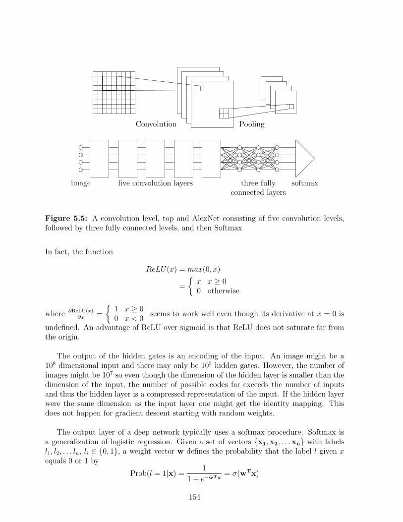
Convolution Pooling

image five convolution layers three fullyconnected layers

softmax

Figure 5.5: A convolution level, top and AlexNet consisting of five convolution levels,followed by three fully connected levels, and then Softmax

In fact, the function

ReLU(x) = max(0, x)

=

x x ≥ 00 otherwise

where ∂ReLU(x)∂x

=

1 x ≥ 00 x < 0

seems to work well even though its derivative at x = 0 is

undefined. An advantage of ReLU over sigmoid is that ReLU does not saturate far fromthe origin.

The output of the hidden gates is an encoding of the input. An image might be a108 dimensional input and there may only be 105 hidden gates. However, the number ofimages might be 107 so even though the dimension of the hidden layer is smaller than thedimension of the input, the number of possible codes far exceeds the number of inputsand thus the hidden layer is a compressed representation of the input. If the hidden layerwere the same dimension as the input layer one might get the identity mapping. Thisdoes not happen for gradient descent starting with random weights.

The output layer of a deep network typically uses a softmax procedure. Softmax isa generalization of logistic regression. Given a set of vectors x1,x2, . . .xn with labelsl1, l2, . . . ln, li ∈ 0, 1, a weight vector w defines the probability that the label l given xequals 0 or 1 by

Prob(l = 1|x) =1

1 + e−wTx= σ(wTx)

154

W1 W2 W3 W4 W5 W6

Figure 5.6: A deep learning fully connected network.

andProb(l = 0|x) = 1− Prob(l = 1/x)

where σ is the sigmoid function.

Define a cost function

J(w) =∑i

(li log(Prob(l = 1|xi)) + (1− li) log(1− Prob(l = 1|xi))

)=∑i

(li log(σ(wTxi)) + (1− li) log(1− σ(wTxi))

)and compute w to minimize J(x). Since ∂σ(wTx)

∂wj= σ(wTx)(1−σ(wTx))xj, it follows that

∂ log(σ(wTx))∂wj

=σ(wTx)(1−σ(wTx))xj

σ(wTx), Thus

∂J

∂wj=∑i

(liσ(wTx)(1− σ(wTx))

σ(wTx)xj − (1− li)

(1− σ(wTx))σ(wTx)

1− σ(wTx)xj

)=∑i

(li(1− σ(wTx))xj − (1− li)σ(wTx)xj

)=∑i

((lixj − liσ(wTx)xj − σ(wTx)xj + liσ(wTx)xj

)=∑i

(li − σ(wTx)

)xj.

Softmax is a generalization of logistic regression to multiple classes. Thus, the labelsli take on values 1, 2, . . . , k. For an input x, softmax estimates the probability of each

155

label. The hypothesis is of the form

hw(x) =

Prob(l = 1|x,w1)Prob(l = 2|x,w2)

...Prob(l = k|x,wk)

=1∑k

i=1 ewT

i x

ew

T1 x

ewT2 x

...

ewTk x

where the matrix formed by the weight vectors is

W = (w1,w2, . . . ,wk)T

W is a matrix since for each label li, there is a vector wi of weights.

Consider a set of n inputs x1,x2, . . . ,xn. Define

δ(l = k) =

1 if l = k0 otherwise

and

J(W ) =n∑i=1

k∑j=1

δ(li = j) logew

Tj xi∑k

h=1 ewT

h xi.

The derivative of the cost function with respect to the weights is

∇wiJ(W ) = −

n∑j=1

xj

(δ(lj = k)− Prob(lj = k)|xj,W

).

Note ∇wiJ(W ) is a vector. Since wi is a vector, each component of ∇wi

J(W ) is thederivative with respect to one component of the vector wi.

Over fitting is a major concern in deep learning since large networks can have hun-dreds of millions of weights. In image recognition, the number of training images canbe significantly increased by random jittering of the images. Another technique calleddropout randomly deletes a fraction of the weights at each training iteration. Regulariza-tion is used to assign a cost to the size of weights and many other ideas are being explored.

Deep learning is an active research area. We explore a few of the directions here. Fora given gate one can construct an activation vector where each coordinate correspondsto an image and the coordinate value is the gate’s output for the corresponding image.Alternatively one could define an image activation vector whose coordinates correspondto gate values for the image.. Basically these activation vectors correspond to rows andcolumns of a matrix whose ijth element is the output of gate i for image j.

A gate activation vector indicates which images an individual gate responds to. Thecoordinates can be permuted so that the activation increases. This then gives the set of

156

images with high activation. To determine whether two gates learn the same feature onecomputes the covariance of the two gate activation vectors.

covariance(ai, aj) =E((ai − E(ai)

)(aj − E(aj)

))σ(ai)σ(aj)

A value close to ±1 indicates a strong relationship between what gates i and j learned.Another interesting question is if a network is trained twice starting from different sets ofrandom weights, do the gates learn the same features or do they carry out the classificationin totally different ways. To match gates that learn the same features one constructs amatrix where the ijth entry is the covariance of the gate i activation vector in one trainingand gate j activation vector in the other training.

Recreating image from activation vectorGiven an image one can easily get the corresponding gate activation vector. However,given a gate activation vector, how does one get the corresponding image. There aremany ways to do this. One way would be to find the gate activation vector for a randomimage and then by gradient descent on the pixels of the image reduce the L2 norm be-tween the gate activation vector of the random image and the gate activation vector forwhich you want the image that produced it.

Style transferGiven that one can produce the image that produced a given activation vector, one canreproduce an image from its content using the style of a different image. To do this definethe content of an image to be the gate activation vector corresponding to the first levelof gates in the network [GEB15]. The reason for selecting the first level of gates is that anetwork discards information in subsequent levels that is not relevant for classification, todefine the style of an image, form a matrix with the inner product of the last activationvector with itself. Now one can create an image using the content of one image and thestyle of another. For example, you could create the image of a student using the style ofa much older individual [GKL+15].

Random weightsAn interesting observation is that one can do style transfer without training a network.One uses random weights instead. This raises the issue of which tasks require trainingand which tasks require only the structure of the network.

Structure of activation spaceUnderstanding the structure of activation space is an important area of research. Onecan examine the region of space that corresponds to images of cats, or one can examinethe the region of space that gets classified as cat. Every input even if it is random noisewill get classified. It appears that every image in one classification is close to an image ineach of the other classifications.

157

FoolingOne can make small changes to an image that will change the image’s classification withoutchanging the image enough for a human to recognize that the image had been modified.There are many ways to do this. To change the classification of an image of a cat toautomobile simply test each pixel value and see which way it increases the probabilityof the image being classified as an automobile. Create a 0,1,-1 matrix where 1 meansincreasing the pixel value increases the likelihood of an automobile classification and a -1means decreasing the pixel value increases the likelihood of an automobile classification.Then

image + α(0,1,-1 matrix)

will cause the modified image to be classified as an automobile for a small value of α.The reason for this is that the change of each pixel value makes a small change in theprobability of the classification but a large number of small changes can be big. For moreinformation about deep learning, see [Ben09].24

5.8.1 Generative Adversarial Networks (GANs)

Image generation has become an important area where one enters a word or phraseinto an image generation program which produces the desired image. One might ask whynot search the web instead? If one wanted an image of a cat, searching the web wouldbe fine. However, if one wants a more complex image of a cat watching someone fishingwhile the sun was setting, it might not be possible to find such an image.

A method that is promising in trying to generate images that look real is to createcode that tries to discern between real images and synthetic images.

imagegenerator

syntheticimage

discriminator

realimage

One first trains the synthetic image discriminator to distinguish between real images andsynthetic ones. Then one trains the image generator to generate images that the discrim-inator believes are real images. Alternating the training between the two units ends upforcing the image generator to produce real looking images. This is the idea of GenerativeAdversarial Networks.

24See also the tutorials: http://deeplearning.net/tutorial/deeplearning.pdf andhttp://deeplearning.stanford.edu/tutorial/.

158

There are many possible applications for this technique. Suppose you wanted to traina network to translate from English to German. First train a discriminator to determineif a sentence is a real sentence as opposed to a synthetic sentence. Then train a translatorfor English to German which translates the English words to German words in such a waythat the output will convince the discriminator that it is a German sentence. Next takethe German sentence and translate it to English words in such as way that the output willconvince the discriminator that it is a English sentence. Finally train the entire systemso the generated English sentence agrees with the original English sentence. At this pointthe German sentence is likely to be a good translation.

translateto German

Input English sentencediscriminator

translateto Englishdiscriminator

compare

5.9 Gradient Descent

The gradient of a function f(x) of d variables, x = (x1, x2, . . . , xd), at a point x0 is de-

noted 5f(x0). It is a d-dimensional vector with components(∂f(x0)∂x1

, ∂f(x0)∂x2

, . . . , ∂f(x0)∂xd

),

where ∂f∂xi

are partial derivatives. Without explicitly stating, we assume that the deriva-tives referred to exist. The rate of increase of the function f as we move from x0 in adirection u is 5f(x0) · u. So the direction of steepest descent is −5f(x0). This is anatural direction to move to minimize f .

By how much should we move? This is primarily an experimental area and how much weshould move depends on the specific problem.. In general one starts with a large moveand when a point is reached where the function no longer decreases since one is possiblyovershooting the minimum, the move size is reduced. Another option is to use a quadraticapproximation and use both the first and second derivatives to determine how far to move.

159

There are significantly improved versions of gradient descent involving momentum andvarious versions of it such as Nesterov’s Accelerated Gradient. If the minimum is in along narrow ravine this may result in an oscillation across the ravine slowing convergencerather than travel along the ravine. Momentum is one method of forcing the move alongthe ravine. The formula is

v = γv + α5 f

x = x− v

Here v is a velocity vector, α is the learning rate, and γ is a constant that is usually setto 0.5 until the initial learning stabilizes and then increased to 0.9. The velocity vectoraverages out the oscillation across the ravine and helps steer the descent in high dimen-sional problems. However, one may not wish to move down the bottom of the narrowravine if the slope is shallow. Although one can improve the training error slightly, onereally wants to improve the true error and avoid over fitting by a regularizer that reducessome measure of complexity.

The step size and how it is changed is important. For educational purposes we nowfocus on infinitesimal gradient descent where the algorithm makes infinitesimal moves inthe −5f(x0) direction. Whenever 5f is not the zero vector, we strictly decrease thefunction in the direction −5f , so the current point is not a minimum of the function.Conversely, a point x where5f = 0 is called a first-order local optimum of f . A first-orderlocal optimum may be a local minimum, local maximum, or a saddle point. We ignoresaddle points since numerical error is likely to prevent gradient descent from stoping ata saddle point at least in low dimensions. In a million dimensions, if there is a decreasein only one dimension and in a million dimensions there is an increase, gradient descentis not likely to find the decrease and stop at the saddle point thinking it is a local minima.

In general, local minima do not have to be global minima, and gradient descent mayconverge to a local minimum that is not a global minimum. When the function f isconvex, this is not the case. A function f of a single variable x is said to be convex iffor any two points a and b, the line joining f(a) and f(b) is above the curve f(·). Afunction of many variables is convex if on any line segment in its domain, it acts as aconvex function of one variable on the line segment.

Definition 5.4 A function f over a convex domain is a convex function if for any twopoints x and y in the domain, and any λ in [0, 1]

f(λx + (1− λ)y

)≤ λf(x) + (1− λ)f(y).

The function is concave if the inequality is satisfied with ≥ instead of ≤.

Theorem 5.18 Suppose f is a convex, differentiable function defined on a closed boundedconvex domain. Then any first-order local minimum is also a global minimum. Infinites-imal gradient descent always reaches the global minimum.

160

Proof: We will prove that if x is a local minimum, then it must be a global minimum.If not, consider a global minimum point y 6= x. On the line joining x and y, the functionmust not go above the line joining f(x) and f(y). This means for an infinitesimal ε > 0,moving distance ε from x towards y, the function must decrease, so 5f(x) is not 0,contradicting the assumption that x is a local minimum.

The second derivatives ∂2

∂xi∂xjform a matrix, called the Hessian, denoted H

(f(x)

).

The Hessian of f at x is a symmetric d× d matrix with ijth entry ∂2f∂xi∂xj

(x). The second

derivative of f at x in the direction u is the rate of change of the first derivative in thedirection u from x. It is easy to see that it equals

uT H(f(x)

)u.

To see this, note that the second derivative of f along the unit vector u is∑j

uj∂

∂xj

(5f(x) · u

)=∑j

uj∑i

∂

∂xj

(ui∂f(x)

∂xi

)=∑j,i

ujui∂2f(x)

∂xj∂xi.

Theorem 5.19 Suppose f is a function from a closed convex domain in Rd to the realsand the Hessian of f exists everywhere in the domain. Then f is convex (concave) on thedomain if and only if the Hessian of f is positive (negative) semi-definite everywhere onthe domain.

Gradient descent requires the gradient to exist. But, even if the gradient is not alwaysdefined, one can minimize a convex function over a convex domain efficiently, i.e., inpolynomial time. Technically, one can only find an approximate minimum with the timedepending on the error parameter as well as the presentation of the convex set. We do notgo into these details. But, in principle we can minimize a convex function over a convexdomain. We can also maximize a concave function over a concave domain. However, ingeneral, we do not have efficient procedures to maximize a convex function over a convexdomain. It is easy to see that at a first-order local minimum of a possibly non-convexfunction, the gradient vanishes. But a second-order local decrease of the function maybe possible. The steepest second-order decrease is in the direction of ±v, where, v is theeigenvector of the Hessian corresponding to the largest absolute valued eigenvalue.

5.9.1 Stochastic Gradient Descent

We now describe a widely-used algorithm in machine learning, called stochastic gradi-ent descent . Often the function f(x) that we are trying to minimize is actually the sumof many simple functions. We may have 100,000 images that we are trying to classify andf(x) =

∑ni=1 f(xi) where f(xi) is the error for the ith image. The function f may have a

161

Error

Weights

Figure 5.7: Error function for a single image

Figure 5.8: Full error function for 1,000 images.

million weights and gradient descent would take the derivation of the 100,000 terms in fwith respect to each of the million weights. A better method might be at each iterationto randomly select one of the images and take the derivatives with respect to just a singleterm in the summation. This should speed the convergence up significantly. In practice,initially one randomly selects one term each iteration, after a number of iterations 50terms are selected, then maybe 200, and finally full gradient descend. This usually getone to a better minimum then the full gradient descent. So not only is it faster but itgets a better solution.

To understand why stochastic gradient descent sometimes gets a better minimum thangradient descent consider Figures 5.7 and 5.8 Here the true error function is the sum of1,000 simpler error functions. If in Figure 5.8 one starts gradient descent at 1000, theyprobably would get stuck at the local minimum around 750. However, stochastic gradientdescent would alternate in minimizing different simple error functions and would moveinto the region 180 to 600 if the batch size was one. If one then switched the batch sizeto 50, the variance would decrease and one might range around 450 to 600. Finally withgradient descent they would converge to a much better minimum.

We have been talking about a local minimum being good in terms of the trainingerror. What we also want is good generalization. If the training data is a good sample of

162

the full data, then intuitively a broad local minimum should be better than a sharp localminimum since a small shift in the error function for a broad minimum will not result ina large increase in error where as a small shift will cause a large increase in error for asharp local minimum.

5.9.2 Regularizer

Often one modifies the error function by adding a regularizer term to achieve some prop-erty. If the amount of data is not sufficient to prevent over fitting one might in traininga deep network add a term that would penalize the number of non-zero weight vectors.A complex network might have 10% training error with 20% real error where as a simplenetwork might have 15% training error with 20% real error. With a regularizer one mightbalance the size of the network with training error and get a training error of 12% andreal error 18%.

5.10 Online Learning

So far we have been considering batch learning. You are given a “batch” of data, atraining sample S, and your goal is to use the training example to produce a hypothesish that will have low error on new data. We now switch to the more challenging onlinelearning scenario where we remove the assumption that data is sampled from a fixedprobability distribution, or from any probabilistic process at all.

The online learning scenario proceeds as follows. At each time t = 1, 2, . . ., two eventsoccur:

1. The algorithm is presented with an arbitrary example xt ∈ X and is asked to makea prediction `t of its label.

2. Then, the algorithm is told the true label of the example c∗(xt) and is charged fora mistake if c∗(xt) 6= `t.

The goal of the learning algorithm is to make as few mistakes as possible. For example,consider an email classifier that when a new email message arrives must classify it as“important” or “it can wait”. The user then looks at the email and informs the algorithmif it was incorrect. We might not want to model email messages as independent randomobjects from a fixed probability distribution because they often are replies to previousemails and build on each other. Thus, the online learning model would be more appro-priate than the batch model for this setting.

Intuitively, the online learning model is harder than the batch model because we haveremoved the requirement that our data consists of independent draws from a fixed proba-bility distribution. Indeed, we will see shortly that any algorithm with good performancein the online model can be converted to an algorithm with good performance in the batch

163

model. Nonetheless, the online model can sometimes be a cleaner model for design andanalysis of algorithms.

5.10.1 An Example: Learning Disjunctions

A disjunction is an OR of features. For example, an email may be important if it comesfrom one of your instructors, or comes from a family member, or is a reply to an emailyou sent earlier. Consider the problem of learning disjunctions over the instance spaceX = 0, 1d, that is, disjunctions over d Boolean features. There are 2d possible disjunc-tions over this instance space, ranging from the disjunction of nothing, which is alwaysnegative, to the disjunction h(x) = x1∨x2∨ ...∨xd that is positive on any example with atleast one feature set to 1. In general, a typical disjunction such as h(x) = x1∨x4∨x8 willhave some relevant variables (in this case, x1, x4, and x8) and some irrelevant variables(in this case, everything else), and outputs positive on any input that has one or morerelevant variables set to 1.

We can solve the problem of learning disjunctions in the online model by startingwith the disjunction of all of the variables h(x) = x1 ∨ x2 ∨ . . . ∨ xd. Our algorithm willmaintain the invariant that every relevant variable for the target function is present in thehypothesis h, along with perhaps some irrelevant variables. This is certainly true at thestart. Given this invariant, the only mistakes possible are on inputs x for which h(x) ispositive but the true label c∗(x) is negative. When such a mistake occurs, we just removefrom h any variable set to 1 in x, since it can’t possibly be a relevant variable for thetarget function. This shrinks the size of the hypothesis h by at least 1, and maintains theinvariant. This implies that the algorithm makes at most d mistakes total on any seriesof examples consistent with a target disjunction c∗. In fact, one can show this boundis tight by showing that no deterministic algorithm can guarantee to make fewer than dmistakes.

Theorem 5.20 For any deterministic online learning algorithm A, there exists a se-quence σ of examples over 0, 1d and a target disjunction c∗ such that A makes at leastd mistakes on the sequence of examples σ labeled by c∗.

Proof: Let σ be the sequence e1, e2, . . . , ed where ej is the example that sets every variableto zero except xj = 1. Imagine running A on sequence σ and telling A it made a mistakeon every example; that is, if A predicts positive on ej we set c∗(ej) = −1 and if A predictsnegative on ej we set c∗(ej) = +1. This target corresponds to the disjunction of all xjsuch that A predicted negative on ej, so it is a legal disjunction. Since A is deterministic,the fact that we constructed c∗ by running A is not a problem: it would make the samemistakes if re-run from scratch on the same sequence and same target. Therefore, Amakes d mistakes on this σ and c∗.

164

5.10.2 The Halving Algorithm

If we are not concerned with running time, a simple online algorithm that guaranteesto make at most log2(|H|) mistakes for a target belonging to any given classH is called thehalving algorithm. This algorithm simply maintains the version space V ⊆ H consistingof all h ∈ H consistent with the labels on every example seen so far, and predicts basedon majority vote over these functions. Each mistake is guaranteed to reduce the size ofthe version space V by at least half (hence the name), thus the total number of mistakesis at most log2(|H|). Note that this can be viewed as the number of bits needed to writea function in H down.

5.10.3 The Perceptron Algorithm

Earlier we described the Perceptron Algorithm as a method for finding a linear sep-arator consistent with a given training set S. However, the Perceptron Algorithm alsooperates naturally in the online setting.

Recall that the basic assumption of the Perceptron Algorithm is that the target func-tion can be described by a vector w∗ such that for each positive example x we havexTw∗ ≥ 1 and for each negative example x we have xTw∗ ≤ −1. Recall also that wecan interpret xTw∗/|w∗| as the distance of x to the hyperplane xTw∗ = 0. Thus, ourassumption states that there exists a linear separator through the origin with all posi-tive examples on one side, all negative examples on the other side, and all examples atdistance at least γ = 1/|w∗| from the separator, where γ is called the margin of separation.

The guarantee of the Perceptron Algorithm will be that the total number of mistakesis at most (r/γ)2 where r = maxt |xt| over all examples xt seen so far. Thus, if there existsa hyperplane through the origin that correctly separates the positive examples from thenegative examples by a large margin relative to the radius of the smallest ball enclosingthe data, then the total number of mistakes will be small. The algorithm, restated in theonline setting, is as follows.

The Perceptron Algorithm: Start with the all-zeroes weight vector w = 0. Then, fort = 1, 2, . . . do:

1. Given example xt, predict sgn(xTt w).

2. If the prediction was a mistake, then update w← w + xtlt.

The Perceptron Algorithm enjoys the following guarantee on its total number of mis-takes.

Theorem 5.21 On any sequence of examples x1,x2, . . ., if there exists a vector w∗ suchthat xTt w∗lt ≥ 1 for all t, i.e., a linear separator of margin γ = 1/|w∗|, then the PerceptronAlgorithm makes at most r2|w∗|2 mistakes, where r = maxt |xt|.

165

Proof: Fix some consistent w∗. Keep track of two quantities, wTw∗ and |w|2. Eachmistake increases wTw∗ by at least 1 since

(w + xtlt)Tw∗ = wTw∗ + xTt ltw

∗ ≥ wTw∗ + 1.

Next, each mistake increases |w|2 by at most r2. For each mistake

(w + xtlt)T (w + xtlt) = |w|2 + 2xTt ltw + |xt|2 ≤ |w|2 + |xt|2 ≤ |w|2 + r2,

where the middle inequality comes from the fact that xTt ltw ≤ 0. Note that it is impor-tant here that we only update on a mistake.

So, if we make m mistakes, then wTw∗ ≥ m, and |w|2 ≤ mr2, or equivalently,|w| ≤ r

√m. Finally, we use the fact that wTw∗/|w∗| ≤ |w| which is just saying that the

projection of w in the direction of w∗ cannot be larger than the length of w. This givesus:

m ≤ wTw∗

m/|w∗| ≤ |w|m/|w∗| ≤ r

√m

√m ≤ r|w∗|m ≤ r2|w∗|2

as desired.

5.10.4 Inseparable Data and Hinge Loss

We assumed above that there exists a perfect w∗ that correctly classifies all the ex-amples, e.g., correctly classifies all the emails into important versus non-important. Thisis rarely the case in real-life data. What if even the best w∗ isn’t perfect? We can seewhat this does to the above proof (Theorem 5.21). If there is an example that w∗ doesn’tcorrectly classify, then while the second part of the proof still holds, the first part (the dotproduct of w with w∗ increasing) breaks down. However, if this doesn’t happen too of-ten, and also xTt w∗ is just a “little bit wrong” then we will only make a few more mistakes.

Define the hinge-loss of w∗ for a positive example xi as the amount xTi w∗ is less thanone and for a negative example xi as the amount xTi w∗ is greater than minus one. Thatis, Lhinge(w

∗, xi) = max(0, 1 − xTi w∗li). The total hinge-loss, Lhinge(w∗, S) for a set of

examples S is the sum of the hinge-loss of each example in S.

Theorem 5.22 On any sequence of examples S = x1,x2, . . ., the Perceptron Algorithmmakes at most

minw∗

(r2|w∗|2 + 2Lhinge(w

∗, S))

mistakes, where r = maxt |xt|.

166

Proof: As before, each update of the Perceptron Algorithm increases |w|2 by at mostr2, so if the algorithm makes m mistakes, we have |w|2 ≤ mr2. What we can no longersay is that each update of the algorithm increases wTw∗ by at least one. Instead, ona positive example we are “increasing” wTw∗ by xTt w∗ (it could be negative), which isat least 1 − Lhinge(w

∗,xt). Similarly, on a negative example we “increase” wTw∗ by−xTt w∗, which is also at least 1−Lhinge(w∗,xt). Summing this up over all mistakes yieldswTw∗ ≥ m− Lhinge(w∗, S), where we are using the fact that hinge-loss is never negativeso summing over all of S is only larger than summing over the mistakes that w made.

Let l = Lhinge(w∗, S). Then

wTw∗ ≤ |w||w∗|(m− l)2 ≤ |w|2|w∗|2

m2 − 2ml + l2 ≤ mr2|w∗|2

m− 2l + l2/m ≤ r2|w∗|2

m ≤ r2|w∗|2 + 2l − l2/mm ≤ r2|w∗|2 + 2l

as desired.

5.10.5 Online to Batch Conversion

Suppose we have an online algorithm with a good mistake bound, such as the Percep-tron Algorithm. Can we use it to get a guarantee in the distributional (batch) learningsetting? Intuitively, the answer should be yes since the online setting is only harder.Indeed, this intuition is correct. We present here two natural approaches for such onlineto batch conversion.

Conversion procedure 1: Random Stopping.Suppose we have an online algorithm A with mistake-bound m. Run the algorithm

in a single pass on a sample S of size m/ε. Let it be the indicator random variable for

the event that A makes a mistake on example xt. Since∑|S|

t=1 it ≤ m for any set S,

E[∑|S|

t=1 it] ≤ m where the expectation is taken over the random draw of S from D|S|. Bylinearity of expectation, and dividing both sides by |S|

1

|S|

|S|∑t=1

E[it] ≤ m/|S| = ε. (5.2)

Let ht denote the hypothesis used by algorithm A to predict on the tth example. Sincethe tth example was randomly drawn from D, E[errD(ht)] = E[it]. This means that if wechoose t at random from 1 to |S|, that is, stopping the algorithm at a random time, theexpected error of the resulting prediction rule, taken over the randomness in the draw ofS and the choice of t, is at most ε as given by equation (5.2). Thus we have the followingtheorem.

167

Theorem 5.23 (Online to Batch via Random Stopping) If an online algorithm Awith mistake-bound m is run on a sample S of size m/ε and stopped at a random timebetween 1 and |S|, the expected error of the hypothesis h produced satisfies E[errD(h)] ≤ ε.

Conversion procedure 2: Controlled Testing.A second approach to using an online learning algorithm A for learning in the distri-

butional setting is as follows. At each step of algorithm A, we test its current hypothesish on a large enough sample to determine if with high probability, the true error of h isless than ε. If h correctly classifies all the examples in the set, then we stop and outputthe hypothesis h. Otherwise, we we select an example x which was misclassified by h andsubmit it to the online algorithm A and get a new hypothesis. We repeat the processuntil we find an h that correctly classifies a large enough sample to ensure with probabil-ity great than or equal to 1−δ, h’s true error will be less than ε. The technical details follow.

Specifically, suppose that the initial hypothesis produced by algorithm A is h1. Defineδi = δ/(i+ 2)2 so

∑∞i=0 δi = (π

2

6− 1)δ ≤ δ. Draw a set of n1 = 1

εlog( 1

δ1) random examples

and test to see whether h1 gets all of them correct. Note that if errD(h1) ≥ ε, then thechance h1 would get them all correct is at most (1− ε)n1 ≤ δ1. So, if h1 indeed gets themall correct, we output h1 as our hypothesis and halt. If not, we choose some examplex1 in the sample on which h1 made a mistake and give it to algorithm A. Algorithm Athen produces some new hypothesis h2 and we again repeat, testing h2 on a fresh set ofn2 = 1

εlog( 1

δ2) random examples, and so on.

In general, given ht we draw a fresh set of nt = 1ε

log( 1δt

) random examples and testto see whether ht gets all of them correct. If so, we output ht and halt; if not, we choosesome xt on which ht(xt) was incorrect and give it to algorithm A. By choice of nt, if hthad error rate ε or larger, the chance we would mistakenly output it is at most δt. Bychoice of the values δt, the chance we ever halt with a hypothesis of error ε or larger is atmost δ1 + δ2 + . . . ≤ δ. Thus, we have the following theorem.

Theorem 5.24 (Online to Batch via Controlled Testing) Let A be an online learn-ing algorithm with mistake-bound m. Then this procedure will halt after O(m

εlog(m

δ))

examples and with probability at least 1− δ will produce a hypothesis of error at most ε.

Note that in this conversion we cannot re-use our samples. Since the hypothesis ht dependson the previous data, we need to draw a fresh set of nt examples to use for testing it.

5.10.6 Combining (Sleeping) Expert Advice

Imagine you have access to a large collection of rules-of-thumb that specify what topredict in different situations. For example, in classifying news articles, you might have arule that says “if the article has the word ‘football’, then classify it as sports” and anotherthat says “if the article contains a dollar figure, then classify it as business”. In predictingthe stock market, there could be different economic indicators. These predictors mightat times contradict each other, e.g., a news article that has both the word “football” and

168

a dollar figure, or a day in which two economic indicators are pointing in different direc-tions. It also may be that no predictor is perfectly accurate with some predictors muchbetter than others. We present here an algorithm for combining a large number of suchpredictors with the guarantee that if any of them are good, the algorithm will performnearly as well as each good predictor on the examples on which that predictor fires.

Formally, define a “sleeping expert” to be a predictor h that on any given example xeither makes a prediction on its label or chooses to stay silent (asleep). Now, suppose wehave access to n such sleeping experts h1, . . . , hn, and let Si denote the subset of exampleson which hi makes a prediction (e.g., this could be articles with the word “football” inthem). We consider the online learning model, and let mistakes(A, S) denote the numberof mistakes of an algorithm A on a sequence of examples S. Then the guarantee of ouralgorithm A will be that for all i

E(mistakes(A, Si)

)≤ (1 + ε)mistakes(hi, Si) +O

(lognε

)where ε is a parameter of the algorithm and the expectation is over internal randomnessin the randomized algorithm A.

As a special case, if h1, . . . , hn are concepts from a concept class H, so they all makepredictions on every example, then A performs nearly as well as the best concept in H.This can be viewed as a noise-tolerant version of the Halving Algorithm of Section 5.10.2for the case that no concept in H is perfect. The case of predictors that make predictionson every example is called the problem of combining expert advice, and the more generalcase of predictors that sometimes fire and sometimes are silent is called the sleeping expertsproblem.

Combining Sleeping Experts Algorithm:

Initialize each expert hi with a weight wi = 1. Let ε ∈ (0, 1). For each example x, do thefollowing:

1. [Make prediction] Let Hx denote the set of experts hi that make a prediction on x, andlet wx =

∑hj∈Hx

wj. Choose hi ∈ Hx with probability pix = wi/wx and predict hi(x).

2. [Receive feedback] Given the correct label, for each hi ∈ Hx let mix = 1 if hi(x) wasincorrect, else let mix = 0.

3. [Update weights] For each hi ∈ Hx, update its weight as follows:

• Let rix =(∑

hj∈Hx pjxmjx

)/(1 + ε)−mix.

• Update wi ← wi(1 + ε)rix .

169

Note that∑

hj∈Hx pjxmjx represents the algorithm’s probability of making a mis-

take on example x. So, hi is rewarded for predicting correctly (mix = 0) when thealgorithm had a high probability of making a mistake, and hi is penalized for pre-dicting incorrectly (mix = 1) when the algorithm had a low probability of makinga mistake.

For each hi 6∈ Hx, leave wi alone.

Theorem 5.25 For any set of n sleeping experts h1, . . . , hn, and for any sequence ofexamples S, the Combining Sleeping Experts Algorithm A satisfies for all i

E(mistakes(A, Si)

)≤ (1 + ε)mistakes(hi, Si) +O

(lognε

)where Si = x ∈ S|hi ∈ Hx.

Proof: Consider sleeping expert hi. The weight of hi after the sequence of examples Sis exactly

wi = (1 + ε)∑x∈Si

[(∑hj∈Hx

pjxmjx

)/(1+ε)−mix

]= (1 + ε)E[mistakes(A,Si)]/(1+ε)−mistakes(hi,Si).

Let w =∑

j wj. Clearly wi ≤ w. Therefore, taking logs:

E(mistakes(A, Si)

)/(1 + ε)−mistakes(hi, Si) ≤ log1+εw.

So, using the fact that log1+εw = O( logWε

),

E(mistakes(A, Si)

)≤ (1 + ε)mistakes(hi, Si) +O

(logwε

).

Initially, w = n. To prove the theorem, it is sufficient to prove that w never increases. Todo so, we need to show that for each x,

∑hi∈Hx wi(1 + ε)rix ≤

∑hi∈Hx wi, or equivalently

dividing both sides by∑

hj∈Hx wj that∑

i pix(1 + ε)rix ≤ 1, where for convenience wedefine pix = 0 for hi 6∈ Hx.

For this we will use the inequalities that for β, z ∈ [0, 1], βz ≤ 1 − (1 − β)z andβ−z ≤ 1 + (1− β)z/β. Specifically, we will use β = (1 + ε)−1. We now have:∑

i

pix(1 + ε)rix =∑i

pixβmix−(

∑j pjxmjx)β

≤∑i

pix

(1− (1− β)mix

)(1 + (1− β)

(∑j

pjxmjx

))

≤

(∑i

pix

)− (1− β)

∑i

pixmix + (1− β)∑i

pix∑j

pjxmjx

= 1− (1− β)∑i

pixmix + (1− β)∑j

pjxmjx

= 1,

170

where the second-to-last line follows from using∑

i pix = 1 in two places. So w neverincreases and the bound follows as desired.

5.11 Boosting

We now describe boosting, which is important both as a theoretical result and as apractical and easy-to-use learning method. A strong learner for a problem is an algorithmthat with high probability is able to achieve any desired error rate ε using a sufficientnumber of samples that may depend polynomially on 1/ε. A weak learner for a problemis an algorithm that does just a little bit better than random guessing. It is only requiredto get with high probability an error rate less than or equal to 1

2− γ for some 0 < γ ≤ 1

2.

We show here that a weak-learner for a problem that achieves the weak-learning guaran-tee for any distribution of data can be boosted to a strong learner, using the techniqueof boosting. At the high level, the idea will be to take our training sample S, and runthe weak-learner on different data distributions produced by weighting the points in thetraining sample in different ways. Running the weak learner on these different weight-ings of the training sample will produce a series of hypotheses h1, h2, . . . . The idea of thereweighting procedure will be to focus attention on the parts of the sample that previoushypotheses have performed poorly on. At the end the hypotheses are combined togetherby a majority vote.

Assume the weak learning algorithm A outputs hypotheses from some class H. Ourboosting algorithm will produce hypotheses that will be majority votes over t0 hypothesesfromH, for t0 defined below. By Theorem 5.13, the class of functions that can be producedby the booster running for t0 rounds has VC-dimensionO(t0VCdim(H) log(t0VCdim(H))).This gives a bound on the number of samples needed, via Corollary 5.17, to ensure thathigh accuracy on the sample will translate to high accuracy on new data.

To make the discussion simpler, assume that the weak learning algorithm A, whenpresented with a weighting of the points in our training sample, always (rather thanwith high probability) produces a hypothesis that performs slightly better than randomguessing with respect to the distribution induced by weighting. Specifically:

Definition 5.5 (γ-Weak learner on sample) A γ-weak learner is an algorithm thatgiven examples, their labels, and a non-negative real weight wi on each example xi, pro-duces a classifier that correctly labels a subset of the examples with total weight at least

(12

+ γ)n∑i=1

wi.

At the high level, boosting makes use of the intuitive notion that if an example wasmisclassified, one needs to pay more attention to it. More specifically, boosting multipliesthe weight of the misclassified examples by a value α > 1 designed to raise their totalweight to equal the total weight of the correctly-classified examples. The boosting proce-dure is in Figure 5.9.

171

Boosting Algorithm

Given a sample S of n labeled examples x1, . . . ,xn, initialize eachexample xi to have a weight wi = 1. Let w = (w1, . . . , wn).

For t = 1, 2, . . . , t0 do

Call the weak learner on the weighted sample (S,w), receivinghypothesis ht.

Multiply the weight of each example that was misclassified by

ht by α =12

+γ12−γ . Leave the other weights as they are.

End

Output the classifier MAJ(h1, . . . , ht0) which takes the majority voteof the hypotheses returned by the weak learner. Assume t0 is odd sothere is no tie.

Figure 5.9: The boosting algorithm

Theorem 5.26 Let A be a γ-weak learner for sample S of n samples. Then t0 =O( 1

γ2log n) is sufficient so that the classifier MAJ(h1, . . . , ht0) produced by the boosting

procedure has training error zero.

Proof: Suppose m is the number of examples the final classifier gets wrong. Each ofthese m examples was misclassified at least t0/2 times so each has weight at least αt0/2.Thus the total weight is at least mαt0/2. On the other hand, at time t+1, only the weightsof examples misclassified at time t were increased. By the property of weak learning, thetotal weight of misclassified examples is at most (1

2− γ) of the total weight at time t. Let

weight(t) be the total weight at time t. Then

weight(t+ 1) ≤(α(

12− γ)

+(

12

+ γ) )× weight(t) = (1 + 2γ)× weight(t).

where α =12

+γ12−γ is the constant that the weights of misclassified examples are multiplied

by. Since weight(0) = n, the total weight at the end is at most n(1 + 2γ)t0 . Thus

mαt0/2 ≤ total weight at end ≤ n(1 + 2γ)t0 .

Substituting α = 1/2+γ1/2−γ = 1+2γ

1−2γand solving for m

m ≤ n(1− 2γ)t0/2(1 + 2γ)t0/2 = n[1− 4γ2]t0/2.

Using 1 − x ≤ e−x, m ≤ ne−2t0γ2 . For t0 >lnn2γ2, m < 1, so the number of misclassified

items must be zero.

172

Having completed the proof of the boosting result, here are two interesting observa-tions:

Connection to Hoeffding bounds: The boosting result applies even if our weak learn-ing algorithm is “adversarial”, giving us the least helpful classifier possible subjectto Definition 5.5. This is why we don’t want the α in the boosting algorithm tobe larger than 0.5+γ

0.5−γ , since in that case the misclassified examples would get highertotal weight than the correctly classified examples, and the weak learner could thenchoose to just return the negation of the classifier it gave the last time. Supposethat the weak learning algorithm gave a classifier each time that for each example,flipped a coin and produced the correct answer with probability 1

2+γ and the wrong

answer with probability 12−γ, so it is a γ-weak learner in expectation. In that case,

if we called the weak learner t0 times, for any fixed xi, Hoeffding bounds imply thechance the majority vote of those classifiers is incorrect on xi is at most e−2t0γ2 . So,the expected total number of mistakes m is at most ne−2t0γ2 . What is interestingis that this is the exact bound we get from boosting without the expectation for anadversarial weak-learner.

A minimax view: Consider a 2-player zero-sum game 25 with one row for each examplexi and one column for each hypothesis hj that the weak-learning algorithm mightoutput. If the row player chooses row i and the column player chooses column j,then the column player gets a payoff of one if hj(xi) is correct and gets a payoffof zero if hj(xi) is incorrect. The γ-weak learning assumption implies that for anyrandomized strategy for the row player (any “mixed strategy” in the language ofgame theory), there exists a response hj that gives the column player an expectedpayoff of at least 1

2+ γ. The von Neumann minimax theorem 26 states that this

implies there exists a probability distribution on the columns (a mixed strategy forthe column player) such that for any xi, at least a 1

2+ γ probability mass of the

columns under this distribution is correct on xi. We can think of boosting as afast way of finding a very simple probability distribution on the columns (just anaverage over O(log n) columns, possibly with repetitions) that is nearly as good (forany xi, more than half are correct) that moreover works even if our only access tothe columns is by running the weak learner and observing its outputs.

We argued above that t0 = O( 1γ2

log n) rounds of boosting are sufficient to produce amajority-vote rule h that will classify all of S correctly. Using our VC-dimension bounds,this implies that if the weak learner is choosing its hypotheses from concept class H, then

25A two person zero sum game consists of a matrix whose columns correspond to moves for Player 1and whose rows correspond to moves for Player 2. The ijth entry of the matrix is the payoff for Player1 if Player 1 choose the jth column and Player 2 choose the ith row. Player 2’s payoff is the negative ofPlayer1’s.

26The von Neumann minimax theorem states that there exists a mixed strategy for each player so thatgiven Player 2’s strategy the best payoff possible for Player 1 is the negative of given Player 1’s strategythe best possible payoff for Player 2. A mixed strategy is one in which a probability is assigned to everypossible move for each situation a player could be in.

173

a sample size

n = O

(1

ε

(VCdim(H)

γ2

))is sufficient to conclude that with probability 1 − δ the error is less than or equal to ε,where we are using the O notation to hide logarithmic factors. It turns out that runningthe boosting procedure for larger values of t0, i.e., continuing past the point where S isclassified correctly by the final majority vote, does not actually lead to greater overfitting.The reason is that using the same type of analysis used to prove Theorem 5.26, one canshow that as t0 increases, not only will the majority vote be correct on each x ∈ S, but infact each example will be correctly classified by a 1

2+ γ′ fraction of the classifiers, where

γ′ → γ as t0 → ∞. That is, the vote is approaching the minimax optimal strategy forthe column player in the minimax view given above. This in turn implies that h can bewell-approximated over S by a vote of a random sample of O(1/γ2) of its component weakhypotheses hj. Since these small random majority votes are not overfitting by much, ourgeneralization theorems imply that h cannot be overfitting by much either.

5.12 Further Current Directions

We now briefly discuss a few additional current directions in machine learning, focusingon semi-supervised learning, active learning, and multi-task learning.

5.12.1 Semi-Supervised Learning

Semi-supervised learning uses a large unlabeled data set U to augment a given labeleddata set L to produce more accurate rules than would have been achieved using just Lalone. In many settings (e.g., document classification, image classification, speech recog-nition), unlabeled data is much more plentiful than labeled data, so one would like tomake use of it. Unlabeled data is missing the labels but often contains information thatan algorithm can take advantage of.

Suppose one believes the target function is a linear separator that separates most ofthe data by a large margin. By observing enough unlabeled data to estimate the proba-bility mass near to any given linear separator, one could in principle discard separatorsin advance that slice through dense regions and instead focus attention on those thatseparate most of the distribution by a large margin. This is the high level idea behinda technique known as Semi-Supervised SVMs. Alternatively, suppose data objects canbe described by two different kinds of features (e.g., a webpage could be described usingwords on the page itself or using words on links pointing to the page), and one believesthat each kind should be sufficient to produce an accurate classifier. Then one might wantto train a pair of classifiers, one on each type of feature, and use unlabeled data for whichone classifier is confident but the other is not to bootstrap, labeling such examples withthe confident classifier and then feeding them as training data to the less-confident one.This is the high-level idea behind a technique known as Co-Training. Or, if one believes

174

“similar examples should generally have the same label”, one might construct a graphwith an edge between examples that are sufficiently similar, and aim for a classifier thatis correct on the labeled data and has a small cut value on the unlabeled data; this is thehigh-level idea behind graph-based methods.

A formal model: The batch learning model introduced in Section 5.4 in essence as-sumes that one’s prior beliefs about the target function be described in terms of a class offunctions H. In order to capture the reasoning used in semi-supervised learning, we needto also describe beliefs about the relation between the target function and the data distri-bution. One way to do this is via a notion of compatibility χ between a hypothesis h anda distribution D. Formally, χ maps pairs (h,D) to [0, 1] with χ(h,D) = 1 meaning that his highly compatible with D and χ(h,D) = 0 meaning that h is highly incompatible withD. For example, if you believe that nearby points should generally have the same label,then if h slices through the middle of a high-density region of D (a cluster), you mightcall h incompatible with D, whereas if no high-density region is split by h then you mightcall it compatible with D. The quantity 1−χ(h,D) is called the unlabeled error rate of h,and denoted errunl(h). Note that for χ to be useful, it must be estimatable from a finitesample; to this end, let us further require that χ is an expectation over individual exam-ples. That is, overloading notation for convenience, we require χ(h,D) = Ex∼D[χ(h, x)],where χ : H×X → [0, 1].

For instance, suppose we believe the target should separate most data by margin γ.We can represent this belief by defining χ(h, x) = 0 if x is within distance γ of the de-cision boundary of h, and χ(h, x) = 1 otherwise. In this case, errunl(h) will denote theprobability mass of D within distance γ of h’s decision boundary. As a different example,in co-training, we assume each example x can be described using two “views” x1 andx2 that each are sufficient for classification. That is, we assume there exist c∗1 and c∗2such that for each example x = 〈x1, x2〉 we have c∗1(x1) = c∗2(x2). We can represent thisbelief by defining a hypothesis h = 〈h1, h2〉 to be compatible with an example 〈x1, x2〉if h1(x1) = h2(x2) and incompatible otherwise; errunl(h) is then the probability mass ofexamples on which h1 and h2 disagree.

As with the class H, one can either assume that the target is fully compatible, i.e.,errunl(c

∗) = 0, or instead aim to do well as a function of how compatible the target is.The case that we assume c∗ ∈ H and errunl(c

∗) = 0 is termed the “doubly realizablecase”. The concept class H and compatibility notion χ are both viewed as known.

Suppose one is given a concept class H (such as linear separators) and a compatibilitynotion χ (such as penalizing h for points within distance γ of the decision boundary).Suppose also that one believes c∗ ∈ H (or at least is close) and that errunl(c

∗) = 0 (or atleast is small). Then, unlabeled data can help by allowing one to estimate the unlabelederror rate of all h ∈ H, thereby in principle reducing the search space from H (all linearseparators) down to just the subset of H that is highly compatible with D. The key

175

challenge is how this can be done efficiently (in theory, in practice, or both) for naturalnotions of compatibility, as well as identifying types of compatibility that data in impor-tant problems can be expected to satisfy.

The following is a semi-supervised analog of our basic sample complexity theorem,Theorem 5.4. First, fix some set of functions H and compatibility notion χ. Given alabeled sample L, define err(h) to be the fraction of mistakes of h on L. Given anunlabeled sample U , define χ(h, U) = Ex∼U [χ(h, x)] and define errunl(h) = 1 − χ(h, U).That is, err(h) and errunl(h) are the empirical error rate and unlabeled error rate of h,respectively. Finally, given α > 0, define HD,χ(α) to be the set of functions f ∈ H suchthat errunl(f) ≤ α.

Theorem 5.27 If c∗ ∈ H, then with probability at least 1 − δ, for labeled set L andunlabeled set U drawn from D, the h ∈ H that optimizes errunl(h) subject to err(h) = 0will have errD(h) ≤ ε for

|U | ≥ 2

ε2

[ln |H|+ ln

4

δ

], and |L| ≥ 1

ε

[ln |HD,χ(errunl(c

∗) + 2ε)|+ ln2

δ

].

Equivalently, for |U | satisfying this bound, for any |L|, whp the h ∈ H that minimizeserrunl(h) subject to err(h) = 0 has

errD(h) ≤ 1

|L|

[ln |HD,χ(errunl(c

∗) + 2ε)|+ ln2

δ

].

Proof: By Hoeffding bounds, |U | is sufficiently large so that with probability at least1− δ/2, all h ∈ H have |errunl(h)− errunl(h)| ≤ ε. Thus we have:

f ∈ H|errunl(f) ≤ errunl(c∗) + ε ⊆ HD,χ(errunl(c

∗) + 2ε).

The given bound on |L| is sufficient so that with probability at least 1− δ, all h ∈ H witherr(h) = 0 and errunl(h) ≤ errunl(c

∗) + ε have errD(h) ≤ ε; furthermore, errunl(c∗) ≤

errunl(c∗) + ε, so such a function h exists. Therefore, with probability at least 1− δ, the

h ∈ H that optimizes errunl(h) subject to err(h) = 0 has errD(h) ≤ ε, as desired.

One can view Theorem 5.27 as bounding the number of labeled examples needed to learnwell as a function of the “helpfulness” of the distribution D with respect to χ. Namely,a helpful distribution is one in which HD,χ(α) is small for α slightly larger than thecompatibility of the true target function, so we do not need much labeled data to identify agood function among those inHD,χ(α). For more information on semi-supervised learning,see [BB10, BM98, CSZ06, Joa99, Zhu06, ZGL03].

5.12.2 Active Learning

Active learning refers to algorithms that take an active role in the selection of which ex-amples are labeled. The algorithm is given an initial unlabeled set U of data points drawn

176

from distribution D and then interactively requests for the labels of a small number ofthese examples. The aim is to reach a desired error rate ε using many fewer labels thanwould be needed by labeling random examples, i.e., passive learning.

Suppose that data consists of points on the real line and H = fa|fa(x) = 1 iff x ≥ afor a ∈ R. That is, H is the set of all threshold functions on the line. It is not hard toshow (see Exercise 5.12) that a random labeled sample of size O(1

εlog(1

δ)) is sufficient to

ensure that with probability greater than or equal to 1 − δ, any consistent threshold a′

has error at most ε. Moreover, it is not hard to show that Ω(1ε) random examples are

necessary for passive learning. Suppose that the data consists of points in the interval[0, 1] where the points in the interval [0, a) are negative and the points in the interval[a, 1] are positive. Given a hypothesis set [b, 1]|0 ≤ b ≤ 1, a random labeled sample ofsize O

(1ε

log 1δ

)is sufficient to ensure that with probability greater than or equal to 1− δ

any hypothesis with zero training error has true error at most ε. However, with activelearning we can achieve error ε using only O

(log(1

ε) + log log(1

δ))

labels. The idea is asfollows. Assume we are given an unlabeled sample U of size O(1

εlog(1

δ)). Now, query the

leftmost and rightmost points. If both are negative, output b = 1. If both are positive,output b = 0. Otherwise (the leftmost is negative and the rightmost is positive), usebinary search to find two adjacent examples x, x′ of U such that x is negative and x′ ispositive, and output b = (x + x′)/2. This threshold b is consistent with the labels onthe entire set U , and so by the above argument, has error less than or equal to ε withprobability greater than or equal to 1− δ.

The agnostic case, where the target need not belong in the given class H is quite a bitmore subtle, and addressed in a quite general way in the “A2” Agnostic Active learningalgorithm [BBL09]. For more information on active learning, see [Das11, BU14].

5.12.3 Multi-Task Learning

In this chapter we have focused on scenarios where our goal is to learn a single targetfunction c∗. However, there are also scenarios where one would like to learn multiple targetfunctions c∗1, c

∗2, . . . , c

∗n. If these functions are related in some way, then one could hope to

do so with less data per function than one would need to learn each function separately.This is the idea of multi-task learning.

One natural example is object recognition. Given an image x, c∗1(x) might be 1 if x isa coffee cup and 0 otherwise; c∗2(x) might be 1 if x is a pencil and 0 otherwise; c∗3(x) mightbe 1 if x is a laptop and 0 otherwise. These recognition tasks are related in that imagefeatures that are good for one task are likely to be helpful for the others as well. Thus,one approach to multi-task learning is to try to learn a common representation underwhich each of the target functions can be described as a simple function. Another naturalexample is personalization. Consider a speech recognition system with n different users.In this case there are n target tasks (recognizing the speech of each user) that are clearly

177

related to each other. Some good references for multi-task learning are [TM95, Thr96].

5.13 Bibliographic Notes

The basic theory underlying learning in the distributional setting was developed by Vap-nik [Vap82], Vapnik and Chervonenkis [VC71], and Valiant [Val84]. The connection ofthis to the notion of Occam’s razor is due to [BEHW87]. For more information on uniformconvergence, regularization and complexity penalization, see [Vap98]. The Perceptron Al-gorithm for online learning of linear separators was first analyzed by Block [Blo62] andNovikoff [Nov62]; the proof given here is from [MP69]. A formal description of the on-line learning model and its connections to learning in the distributional setting is givenin [Lit87]. Support Vector Machines and their connections to kernel functions were firstintroduced by [BGV92], and extended by [CV95], with analysis in terms of margins givenby [STBWA98]. For further reading on SVMs, learning with kernel functions, and regu-larization, see [SS01]. VC dimension is due to Vapnik and Chervonenkis [VC71] with theresults presented here given in Blumer, Ehrenfeucht, Haussler and Warmuth [BEHW89].Boosting was first introduced by Schapire [Sch90], and Adaboost and its guarantees aredue to Freund and Schapire [FS97] . Analysis of the problem of combining expert advicewas given by Littlestone and Warmuth [LW94] and Cesa-Bianchi et al. [CBFH+97]; theanalysis of the sleeping experts problem given here is from [BM07].

178

5.14 Exercises

Exercise 5.1 Each of the following data sets consists of a subset of the d-dimensional0/1 vectors labeled +1. The remaining 0/1 vectors are labeled -1. Which sets are linearlyseparable?

1. 010, 011, 100, 111

2. 011, 100, 110, 111

3. 0100, 0101, 0110, 1000, 1100, 1101, 1110, 1111

Exercise 5.2 Run the Perceptron Algorithm on each of the examples in Exercise 5.1.What happens?

Exercise 5.3 (representation and linear separators) A logical disjunction is the orof a set of Boolean variables such as x1 ∨ x2 ∨ x4. Show that any disjunction over 0, 1dcan be represented as a linear separator. Show that moreover the margin of separation isΩ(1/

√d).

Exercise 5.4 (representation and linear separators) Show that the parity functionon d ≥ 2 Boolean variables cannot be represented by a linear threshold function. Theparity function is 1 if and only if an odd number of inputs is 1.

Exercise 5.5 Given two sets of d dimensional vectors S1 and S2 how would you determineif the convex hulls of the two sets intersected?

Solution: Use perceptron algorithm.

Exercise 5.6 (kernels) Prove Theorem 5.3.

Exercise 5.7 Find the mapping ϕ(x) that gives rise to the kernel

K(x,y) = (x1y1 + x2y2)2.

Exercise 5.8 Give an example of overfitting, that is, where training error is much lessthan true error.

Exercise 5.9 One popular practical method for machine learning is to learn a decisiontree (Figure 5.10). While finding the smallest decision tree that fits a given training sampleS is NP-hard, there are a number of heuristics that are used in practice. Suppose we runsuch a heuristic on a training set S and it outputs a tree with k nodes. Show that such atree can be described using O(k log d) bits, where d is the number of features. Assume allfeatures are binary valued (as in Figure 5.10). By Theorem 5.7, we can be confident thetrue error is low if we can produce a consistent tree with fewer than ε|S|/ log(d) nodes.

179

Figure 5.10: A decision tree with three internal nodes and four leaves. This tree corre-sponds to the Boolean function x1x2 ∨ x1x2x3 ∨ x2x3.

Exercise 5.10 Consider the class of OR-functions (disjunctions) over d binary (0/1-valued) features. For instance, one such OR-function is x1 ∨ x2 ∨ x4. Using Theorem 5.4,how many examples are sufficient so that with probability at least 1−δ, only OR-functionsof true error less than ε will have zero training error?

Exercise 5.11 Consider the instance space X = 0, 1d and let H be the class of 3-CNFformulas. That is, H is the set of concepts that can be described as a conjunction of clauseswhere each clause is an OR of up to 3 literals. (These are also called 3-SAT formulas).For example c∗ might be (x1 ∨ x2 ∨ x3)(x2 ∨ x4)(x1 ∨ x3)(x2 ∨ x3 ∨ x4). Assume we arein the PAC learning setting, so examples are drawn from some underlying distribution Dand labeled by some 3-CNF formula c∗.

1. Give a number of samples m that would be sufficient to ensure that with probabilitygreater than or equal to 1− δ, all 3-CNF formulas consistent with the sample haveerror at most ε with respect to D.

2. Give a polynomial-time algorithm that finds a 3-CNF formula consistent with thesample if one exists.

Exercise 5.12 Consider an instance space X consisting of integers 1 to 1,000,000 and atarget concept c∗ where c∗(i) = 1 for 500001 ≤ i ≤ 1000000. If your hypothesis class H ishj|hj(i) = 1 for i ≥ j and hj(i) = 0 for i < j how large a training set S do you need toinsure that with probability 99% any consistent hypothesis in H will have true error lessthan 10%.

Exercise 5.13 Consider a deep network with 100,000 parameters each given by a 32-bitfloating point number. Suppose the network is trained on 100,000,000 training examples.Corollary 5.8 says that with probability 99.9% the true error will differ from the empiricalerror by some ε. What is the value of ε?

Exercise 5.14 (Regularization) Pruning a decision tree: Let S be a labeled sampledrawn iid from some distribution D over 0, 1n, and suppose S was used to create

180

some decision tree T . However, the tree T is large, and we might be overfitting. Givea polynomial-time algorithm for pruning T that finds the pruning h of T that optimizesthe right-hand-side of Corollary 5.8, i.e., that for a given δ > 0 minimizes:

errS(h) +

√size(h) ln(4) + ln(2/δ)

2|S|.

To discuss this, we define the meaning of “pruning” of T and the meaning of “size” ofh. A pruning h of T is a tree in which some internal nodes of T have been turned intoleaves, labeled “+” or “−” depending on whether the majority of examples in S that reachthat node are positive or negative. Let size(h) = L(h) log(n) where L(h) is the number ofleaves in h.

Hint #1: it is sufficient, for each integer L = 1, 2, . . . , L(T ), to find the pruning of Twith L leaves of lowest empirical error on S, that is, hL = argminh:L(h)=LerrS(h). Thenplug them all into the displayed formula above and pick the best formula.

Hint #2: use dynamic programming.

Exercise 5.15 Consider the instance space X = R2. What is the VC-dimension of rightcorners with axis aligned edges that are oriented with one edge going to the right and theother edge going up?

Exercise 5.16 (VC-dimension; Section 5.5) What is the VC-dimension V of theclass H of axis-parallel boxes in Rd? That is, H = ha,b|a,b ∈ Rd where ha,b(x) = 1 ifai ≤ xi ≤ bi for all i = 1, . . . , d and ha,b(x) = −1 otherwise. Select a set of points V thatis shattered by the class and

1. prove that the VC-dimension is at least |V | by proving V shattered, and

2. prove that the VC-dimension is at most |V | by proving that no set of |V |+ 1 pointscan be shattered.

Exercise 5.17 VC-dimension Prove that the VC-dimension of circles in the plane isthree.

Exercise 5.18 (VC-dimension, Perceptron, and Margins) A set of points S is“shattered by linear separators of margin γ” if every labeling of the points in S is achievableby a linear separator of margin at least γ. Prove that no set of 1/γ2 + 1 points in the unitball is shattered by linear separators of margin γ.Hint: think about the Perceptron Algorithm and try a proof by contradiction.

Exercise 5.19 Given two fully connected levels without a non-linear element, one cancombine the two levels into one level. Can this be done for two convolution levels withoutpooling and without a nonlinear element?

181

Exercise 5.20 At present there are many interesting research directions in deep learningthat are being explored. This exercise focuses on whether gates in networks learn the samething independent of the architecture or how the network is trained. On the web thereare several copies of Alexnet that have been trained starting from different random initialweights. Select two copies and form a matrix where the columns of the matrix correspondto gates in the first copy of Alexnet and the rows of the matrix correspond to gates ofthe same level in the second copy. The ijth entry of the matrix is the covariance of theactivation of the jth gate in the first copy of Alexnet with the ith gate in the second copy.The covariance is the expected value over all images in the data set.

1. Match the gates in the two copies of the network using a bipartite graph matchingalgorithm. What is the fraction of matches that have a high covariance?

2. It is possible that there is no good one to one matching of gates but that some smallset of gates in the first copy of the network learn what some small set of gates in thesecond copy learn. Explore a clustering technique to match sets of gates and carryout an experiment to do this.

Exercise 5.21

1. Input an image to a deep learning network. Reproduce the image from the activationvector, aimage, it produced by inputting a random image and producing an activationvector arandom. Then by gradient descent modify the pixels in the random image tominimize the error function |aimage − arandom|2.

2. Train a deep learning network to produce an image from an activation network.

Exercise 5.22

1. Create and train a simple deep learning network consisting of a convolution level withpooling, a fully connected level, and then softmax. Keep the network small. For inputdata use the MNIST data set http://yann.lecun.com/exdb/mnist/ with 28×28images of digits. Use maybe 20 channels for the convolution level and 100 gates forthe fully connected level.

2. Create and train a second network with two fully connected levels, the first level with200 gates and the second level with 100 gates. How does the accuracy of the secondnetwork compare to the first?

3. Train the second network again but this time use the activation vector of the 100gate level and train the second network to produce that activation vector and onlythen train the softmax. How does the accuracy compare to direct training of thesecond network and the first network?

182

convolution

first network second network

Exercise 5.23 (Perceptron and Stochastic Gradient Descent) We know the Per-ceptron Algorithm makes at most 1/γ2 updates on any sequence of examples that is sep-arable by margin γ (assume all examples have length at most 1). However, it need notfind a separator of large margin. If we also want to find a separator of large margin, anatural alternative is to update on any example xi such that li(w · xi) < 1; this is calledthe margin perceptron algorithm.

1. Argue why margin perceptron is equivalent to running stochastic gradient descentwith learning rate 1 (on each example, add the negative gradient of the loss functionto the current weight vector) on the class of linear predictors with hinge-loss as theloss function.

2. Prove that on any sequence of examples that are separable by margin γ, this algorithmwill make at most 3/γ2 updates.

3. In Part 2 you probably proved that each update increases |w|2 by at most 3. Use thisand your result from Part 2 to conclude that if you have a dataset S that is separableby margin γ, and cycle through the data until the margin perceptron algorithm makesno more updates, that it will find a separator of margin at least γ/3.

Exercise 5.24 Consider running the Perceptron Algorithm in the online model on somesequence of examples S. Let S ′ be the same set of examples as S but presented in a differentorder. Does the Perceptron Algorithm necessarily make the same number of mistakes onS as it does on S ′? If so, why? If not, show such an S and S ′ consisting of the same setof examples in a different order where the Perceptron Algorithm makes a different numberof mistakes on S ′ than it does on S.

Exercise 5.25 (Sleeping Experts and Decision trees) “Pruning” a Decision TreeOnline via Sleeping Experts: Suppose that, as in Exercise 5.14, we are given a decision treeT , but now we are faced with a sequence of examples that arrive online. One interestingway we can make predictions is as follows. For each node v of T (internal node or leaf)create two sleeping experts: one that predicts positive on any example that reaches v andone that predicts negative on any example that reaches v. So, the total number of sleepingexperts is equal to the number of nodes of T which is proportional to the number of leavesL(T ) of T .

183

1. Say why any pruning h of T , and any assignment of +,− labels to the leaves of h,corresponds to a subset of sleeping experts with the property that exactly one sleepingexpert in the subset makes a prediction on any given example.

2. Prove that for any sequence S of examples, and any given number of leaves L, if

we run the sleeping-experts algorithm using ε =√

L log(L(T ))|S| , then the expected error

rate of the algorithm on S (the total number of mistakes of the algorithm divided by

|S|) will be at most errS(hL) + O(√

L log(L(T ))|S| ), where hL = argminh:L(h)=LerrS(h)

is the pruning of T with L leaves of lowest error on S.

3. In the above question, we assumed L was given. Explain how we can remove this as-

sumption and achieve a bound of minL

[errS(hL) +O(

√L log(L(T ))|S| )

]by instantiating

L(T ) copies of the above algorithm (one for each value of L) and then combiningthese algorithms using the experts algorithm (in this case, none of them will besleeping).

Exercise 5.26 (Boosting) Consider the boosting algorithm given in Figure 5.9. Supposehypothesis ht has error rate βt on the weighted sample (S,w) for βt much less than 1

2− γ.

Then, after the booster multiples the weight of misclassified examples by α, hypothesis htwill still have error less than 1

2− γ under the new weights. This means that ht could be

given again to the booster (perhaps for several times in a row). Calculate, as a function ofα and βt, approximately how many times in a row ht could be given to the booster beforeits error rate rises to above 1

2− γ. You may assume βt is much less than 1

2− γ.

Note: The AdaBoost boosting algorithm [FS97] can be viewed as performing this ex-periment internally, multiplying the weight of misclassified examples by αt = 1−βt

βt, and

then giving ht a weight proportional to the quantity you computed in its final majority-votefunction.

184

6 Algorithms for Massive Data Problems: Stream-

ing, Sketching, and Sampling

6.1 Introduction

This chapter deals with massive data problems where the input data is too large to bestored in random access memory. One model for such problems is the streaming model,where n data items a1, a2, . . . , an arrive one at a time. For example, the ai might beIP addresses being observed by a router on the internet. The goal is to compute somestatistics, property, or summary of these data items without using too much memory,much less than n. More specifically, we assume each ai itself is a b-bit quantity where b isnot too large. For example, each ai might be an integer, 1 ≤ ai ≤ m, where m = 2b. Thegoal is to produce some desired output using space polynomial in b and log n; see Figure6.1.

For example, a very easy problem to solve in the streaming model is to compute thesum of the ai. If each ai is an integer between 1 and m = 2b, then the sum of all the ai isan integer between 1 and mn and so the number of bits of memory needed to maintainthe sum is O(b + log n). A harder problem, discussed shortly, is computing the numberof distinct numbers in the input sequence.

One natural approach for tackling a range of problems in the streaming model is toperform random sampling of the input “on the fly”. To introduce the basic flavor ofsampling on the fly, consider a stream a1, a2, . . . , an from which we are to select an indexi with probability proportional to the value of ai. When we see an element, we do notknow the probability with which to select it since the normalizing constant depends onall of the elements including those we have not yet seen. However, the following methodworks. Let s be the sum of the ai’s seen so far. Maintain s and an index i selected withprobability ai

s. Initially i = 1 and s = a1. Having seen symbols a1, a2, . . . , aj, s will equal

a1 + a2 + · · ·+ aj and for i in 1, . . . , j, the selected index will be i with probability ais

.On seeing aj+1, change the selected index to j + 1 with probability

aj+1

s+aj+1and otherwise

keep the same index as before with probability 1− aj+1

s+aj+1. If we change the index to j + 1,

clearly it was selected with the correct probability. If we keep i as our selection, then itwill have been selected with probability(

1− aj+1

s+ aj+1

)ais

=s

s+ aj+1

ais

=ai

s+ aj+1

which is the correct probability for selecting index i. Finally s is updated by adding aj+1

to s. This problem comes up in many areas such as sleeping experts where there is asequence of weights and we want to pick an expert with probability proportional to itsweight. The ai’s are the weights and the subscript i denotes the expert.

185

stream a1, a2, . . . , an Algorithm(low space)

some output

Figure 6.1: High-level representation of the streaming model

6.2 Frequency Moments of Data Streams

An important class of problems concerns the frequency moments of data streams. Asmentioned above, a data stream a1, a2, . . . , an of length n consists of symbols ai froman alphabet of m possible symbols, which for convenience we denote as 1, 2, . . . ,m.Throughout this section, n,m, and ai will have these meanings and s (for symbol) willdenote a generic element of 1, 2, . . . ,m. The frequency fs of the symbol s is the numberof occurrences of s in the stream. For a non-negative integer p, the pth frequency momentof the stream is

m∑s=1

fps .

Note that the p = 0 frequency moment corresponds to the number of distinct symbolsoccurring in the stream using the convention 00 = 0. The first frequency moment is justn, the length of the string. The second frequency moment,

∑s f

2s , is useful in computing

the variance of the stream, i.e., the average squared difference from the average frequency.

1

m

m∑s=1

(fs −

n

m

)2

=1

m

m∑s=1

(f 2s − 2

n

mfs +

( nm

)2)

=

(1

m

m∑s=1

f 2s

)− n2

m2

In the limit as p becomes large,

(m∑s=1

fps

)1/p

is the frequency of the most frequent ele-

ment(s).

We will describe sampling based algorithms to compute these quantities for streamingdata shortly. First a note on the motivation for these problems. The identity and fre-quency of the the most frequent item, or more generally, items whose frequency exceeds agiven fraction of n, is clearly important in many applications. If the items are packets ona network with source and/or destination addresses, the high frequency items identify theheavy bandwidth users. If the data consists of purchase records in a supermarket, the highfrequency items are the best-selling items. Determining the number of distinct symbolsis the abstract version of determining such things as the number of accounts, web users,or credit card holders. The second moment and variance are useful in networking as wellas in database and other applications. Large amounts of network log data are generatedby routers that can record the source address, destination address, and the number ofpackets for all the messages passing through them. This massive data cannot be easilysorted or aggregated into totals for each source/destination. But it is important to know

186

if some popular source-destination pairs have a lot of traffic for which the variance is onenatural measure.

6.2.1 Number of Distinct Elements in a Data Stream

Consider a sequence a1, a2, . . . , an of n elements, each ai an integer in the range 1 to mwhere n and m are very large. Suppose we wish to determine the number of distinct ai inthe sequence. Each ai might represent a credit card number extracted from a sequence ofcredit card transactions and we wish to determine how many distinct credit card accountsthere are. Note that this is easy to do in O(m) space by just storing a bit-vector thatrecords which elements have been seen so far and which have not. It is also easy to do inO(n logm) space by storing a list of all distinct elements that have been seen. However,our goal is to use space logarithmic in m and n. We first show that this is impossibleusing an exact deterministic algorithm. Any deterministic algorithm that determines thenumber of distinct elements exactly must use at least m bits of memory on some inputsequence of length O(m). We then will show how to get around this problem using ran-domization and approximation.

Lower bound on memory for exact deterministic algorithm We show that anyexact deterministic algorithm must use at least m bits of memory on some sequence oflength m+ 1. Suppose we have seen a1, . . . , am, and our algorithm uses less than m bitsof memory on all such sequences. There are 2m − 1 possible subsets of 1, 2, . . . ,m thatthe sequence could contain and yet only 2m−1 possible states of our algorithm’s memory.Therefore there must be two different subsets S1 and S2 that lead to the same memorystate. If S1 and S2 are of different sizes, then clearly this implies an error for one of theinput sequences. On the other hand, if they are the same size and the next element is inS1 but not S2, the algorithm will give the same answer in both cases and therefore mustgive an incorrect answer on at least one of them.

Algorithm for the number of distinct elements To beat the above lower bound,consider approximating the number of distinct elements. Our algorithm will produce anumber that is within a constant factor of the correct answer using randomization andthus a small probability of failure. Suppose the set S of distinct elements was chosenuniformly at random from 1, . . . ,m. Let min denote the minimum element in S. Whatis the expected value of min? If there was one distinct element, then its expected valuewould be roughly m

2. If there were two distinct elements, their expected value would be

roughly m3

. More generally, for a random set S, the expected value of the minimum isapproximately m

|S|+1. See Figure 6.2. Solving min = m

|S|+1yields |S| = m

min− 1. This

suggests keeping track of the minimum element in O(logm) space and using this equationto give an estimate of |S|.

Converting the intuition into an algorithm via hashing In general, the set Smight not have been chosen uniformly at random. If the elements of S were obtained

187

m|S|+1

︷ ︸︸ ︷|S|+ 1 subsets

Figure 6.2: Estimating the size of S from the minimum element in S which has valueapproximately m

|S|+1. The elements of S partition the set 1, 2, . . . ,m into |S|+ 1 subsets

each of size approximately m|S|+1

.

by selecting the |S| smallest elements of 1, 2, . . . ,m, the above technique would give avery bad answer. However, we can convert our intuition into an algorithm that workswell with high probability on every sequence via hashing. Specifically, we will use a hashfunction h where

h : 1, 2, . . . ,m → 0, 1, 2, . . . ,M − 1 ,

and then instead of keeping track of the minimum element ai ∈ S, we will keep track ofthe minimum hash value. The question now is: what properties of a hash function dowe need? Since we need to store h, we cannot use a totally random mapping since thatwould take too many bits. Luckily, a pairwise independent hash function, which can bestored compactly is sufficient.

We recall the formal definition of pairwise independence below. But first recall thata hash function is always chosen at random from a family of hash functions and phraseslike “probability of collision” refer to the probability in the choice of hash function.

2-Universal (Pairwise Independent) Hash Functions Various applications use dif-ferent amounts of randomness. Full randomness for a vector x = (x1, x2, . . . xd) whereeach xi ∈ 0, 1 would require selecting x uniformly at random from the set of all 2d 0,1vectors. However, if we only need that each xi be equally likely to be 0 or 1, we can selectx from the set of two vectors (0, 0, . . . , 0), (1, 1, . . . , 1). If in addition, we want each pairof coordinates xi and xj to be statistically independent, we need a larger set to chose fromwhich has the property that for each pair i and j, (xi, xj) is equally likely to be (0,0),(0,1), (1,0) or (1,1).

A set of hash functions

H =h | h : 1, 2, . . . ,m → 0, 1, 2, . . . ,M − 1

is 2-universal or pairwise independent if for all x and y in 1, 2, . . . ,m with x 6= y,h(x) and h(y) are each equally likely to be any element of 0, 1, 2, . . . ,M − 1 and arestatistically independent. It follows that a set of hash functions H is 2-universal if andonly if for all x and y in 1, 2, . . . ,m, x 6= y, h(x) and h(y) are each equally likely to be

188

any element of 0, 1, 2, . . . ,M − 1, and for all w and z

Probh∼H

(h (x) = w and h (y) = z

)= 1

M2 .

We now give an example of a 2-universal family of hash functions. Let M be a primegreater than m. For each pair of integers a and b in the range [0,M − 1], define a hashfunction

hab (x) = ax+ b (mod M).

To store the hash function hab, store the two integers a and b. This requires only O(logM)space. To see that the family is 2-universal note that h(x) = w and h(y) = z if and onlyif (

x 1y 1

)(ab

)=

(wz

)(mod M).

If x 6= y, the matrix

(x 1y 1

)is invertible modulo M .27 Thus

(a

b

)=

(x 1y 1

)−1(w

z

)(mod M)

and for each(wz

)there is a unique

(ab

). Hence

Prob(h(x) = w and h(y) = z

)=

1

M2

and H is 2-universal.

Analysis of distinct element counting algorithm Let b1, b2, . . . , bd be the distinctvalues that appear in the input. Select h from the 2-universal family of hash functions H.Then the set S = h(b1), h(b2), . . . , h(bd) is a set of d random and pairwise independentvalues from the set 0, 1, 2, . . . ,M − 1. We now show that M

minis a good estimate for d,

the number of distinct elements in the input, where min = min(S).

Lemma 6.1 With probability at least 23− d

M, the estimate of the number of distinct

elements satisfies, d6≤ M

min≤ 6d, where min is the smallest element of S. That is,

M6d≤ min ≤ 6M

d.

Proof: First, we show that Prob(min ≤ M

6d

)≤ 1

6+ dM

. This part does not require pairwiseindependence.

Prob

(min ≤ M

6d

)= Prob

(∃k, h (bk) ≤

M

6d

)≤

d∑i=1

Prob

(h(bi) ≤

M

6d

)≤ d

(dM

6de

M

)≤ d

(1

6d+

1

M

)≤ 1

6+

d

M.

27The primality of M ensures that inverses of elements exist in Z∗M and M > m ensures that if x 6= y,

then x and y are not equal mod M .

189

t

M6d

Md

6Md︸ ︷︷ ︸

Min here ifthere existsi, h(bi) ≤ M

6d

︸ ︷︷ ︸Min hereif for all i,h(bi) ≥ 6M

d

Figure 6.3: Location of the minimum in the distinct counting algorithm.

Next, we show that Prob(min ≥ 6M

d

)≤ 1

6. This part will use pairwise independence.

First,Prob

(min ≥ 6M

d

)= Prob

(∀k, h (bk) ≥ 6M

d

).

For i = 1, 2, . . . , d, define the indicator variable

yi =

0 if h (bi) ≥ 6M

d

1 otherwise

and let

y =d∑i=1

yi.

We want to show that Prob(y = 0) is small. Now Prob (yi = 1) ≥ 6d, E (yi) ≥ 6

d, and

E (y) ≥ 6. For 2-way independent random variables, the variance of their sum is thesum of their variances. So Var (y) = dVar (y1). Further, since y1 is 0 or 1, Var(y1) =E[(y1 − E(y1))2] = E(y2

1) − E2(y1) = E(y1) − E2(y1) ≤ E (y1) . Thus Var(y) ≤ E (y).By the Chebyshev inequality,

Prob(min ≥ 6M

d

)= Prob

(∀k h (bk) ≥

6M

d

)= Prob (y = 0)

≤ Prob (|y − E (y)| ≥ E (y))

≤ Var(y)

E2 (y)≤ 1

E (y)≤ 1

6

Since Mmin≥ 6d with probability at most 1

6+ d

Mand M

min≤ d

6with probability at most 1

6,

d6≤ M

min≤ 6d with probability at least 2

3− d

M.

6.2.2 Number of Occurrences of a Given Element.

To count the number of occurrences of a given element in a stream requires at mostlog n space where n is the length of the stream. Clearly, for any length stream that occurs

190

in practice, one can afford log n space. For this reason, the following material may neverbe used in practice, but the technique is interesting and may give insight into how to solvesome other problem.

Consider a string of 0’s and 1’s of length n in which we wish to count the number ofoccurrences of 1’s. Clearly with log n bits of memory we could keep track of the exactnumber of 1’s. However, the number can be approximated with only log log n bits.

Let m be the number of 1’s that occur in the sequence. Keep a value k such that 2k

is approximately the number m of occurrences. Storing k requires only log log n bits ofmemory. The algorithm works as follows. Start with k=0. For each occurrence of a 1,add one to k with probability 1/2k. At the end of the string, the quantity 2k − 1 is theestimate of m. To obtain a coin that comes down heads with probability 1/2k, flip a faircoin, one that comes down heads with probability 1/2, k times and report heads if the faircoin comes down heads in all k flips.

Given k, on average it will take 2k ones before k is incremented. Thus, the expectednumber of 1’s to produce the current value of k is 1 + 2 + 4 + · · ·+ 2k−1 = 2k − 1.

6.2.3 Frequent Elements

The Majority and Frequent Algorithms First consider the very simple problem ofn people voting. There are m candidates, 1, 2, . . . ,m. We want to determine if onecandidate gets a majority vote and if so who. Formally, we are given a stream of integersa1, a2, . . . , an, each ai belonging to 1, 2, . . . ,m, and want to determine whether there issome s ∈ 1, 2, . . . ,m which occurs more than n/2 times and if so which s. It is easy tosee that to solve the problem exactly on read-once streaming data with a deterministicalgorithm, requires Ω(min(n,m)) space. Suppose n is even and the last n/2 items areidentical. Suppose also that after reading the first n/2 items, there are two different setsof elements that result in the same content of our memory. In that case, a mistake wouldoccur if the second half of the stream consists solely of an element that is in one set, butnot in the other. If n/2 ≥ m then there are at least 2m − 1 possible subsets of the first

n/2 elements. If n/2 ≤ m then there are∑n/2

i=1

(mi

)subsets. By the above argument, the

number of bits of memory must be at least the base 2 logarithm of the number of subsets,which is Ω(min(m,n)).

Surprisingly, we can bypass the above lower bound by slightly weakening our goal.Again let’s require that if some element appears more than n/2 times, then we mustoutput it. But now, let us say that if no element appears more than n/2 times, then ouralgorithm may output whatever it wants, rather than requiring that it output “no”. Thatis, there may be “false positives”, but no “false negatives”.

Majority Algorithm

191

Store a1 and initialize a counter to one. For each subsequent ai, if ai is thesame as the currently stored item, increment the counter by one. If it differs,decrement the counter by one provided the counter is non-zero. If the counteris zero, then store ai and set the counter to one.

To analyze the algorithm, it is convenient to view the decrement counter step as “elim-inating” two items, the new one and the one that caused the last increment in the counter.It is easy to see that if there is a majority element s, it must be stored at the end. Ifnot, each occurrence of s was eliminated; but each such elimination also causes anotheritem to be eliminated. Thus for a majority item not to be stored at the end, more thann items must have eliminated, a contradiction.

Next we modify the above algorithm so that not just the majority, but also itemswith frequency above some threshold are detected. More specifically, the algorithm belowfinds the frequency (number of occurrences) of each element of 1, 2, . . . ,m to within anadditive term of n

k+1. That is, for each symbol s, the algorithm produces a value fs in

[fs − nk+1

, fs], where fs is the true number of occurrences of symbol s in the sequence.It will do so using O(k log n + k logm) space by keeping k counters instead of just onecounter.

Algorithm Frequent

Maintain a list of items being counted. Initially the list is empty. For eachitem, if it is the same as some item on the list, increment its counter by one.If it differs from all the items on the list, then if there are less than k itemson the list, add the item to the list with its counter set to one. If there arealready k items on the list, decrement each of the current counters by one.Delete an element from the list if its count becomes zero.

Theorem 6.2 At the end of Algorithm Frequent, for each s ∈ 1, 2, . . . ,m, its counteron the list fs satisfies fs ∈ [fs − n

k+1, fs]. If some s does not occur on the list, its counter

is zero and the theorem asserts that fs ≤ nk+1

.

Proof: The fact that fs ≤ fs is immediate. To show fs ≥ fs− nk+1

, view each decrementcounter step as eliminating some items. An item is eliminated if the current ai being readis not on the list and there are already k symbols different from it on the list; in this case, aiand k other distinct symbols are simultaneously eliminated. Thus, the elimination of eachoccurrence of an s ∈ 1, 2, . . . ,m is really the elimination of k + 1 items correspondingto distinct symbols. Thus, no more than n/(k + 1) occurrences of any symbol can beeliminated. It is clear that if an item is not eliminated, then it must still be on the list atthe end. This proves the theorem.

Theorem 6.2 implies that we can compute the true frequency of every s ∈ 1, 2, . . . ,mto within an additive term of n

k+1.

192

6.2.4 The Second Moment

This section focuses on computing the second moment of a stream with symbols from1, 2, . . . ,m. Let fs denote the number of occurrences of the symbol s in the stream,and recall that the second moment of the stream is given by

∑ms=1 f

2s . To calculate the

second moment, for each symbol s, 1 ≤ s ≤ m, independently set a random variable xsto ±1 with probability 1/2. In particular, think of xs as the output of a random hashfunction h(s) whose range is just the two buckets −1, 1. For now, think of h as a fullyindependent hash function. Maintain a sum by adding xs to the sum each time the symbols occurs in the stream. At the end of the stream, the sum will equal

∑ms=1 xsfs. The

expected value of the sum will be zero where the expectation is over the choice of the ±1value for the xs.

E

(m∑s=1

xsfs

)= 0

Although the expected value of the sum is zero, its actual value is a random variable andthe expected value of the square of the sum is given by

E

(m∑s=1

xsfs

)2

= E

(m∑s=1

x2sf

2s

)+ 2E

(∑s 6=t

xsxtfsft

)=

m∑s=1

f 2s ,

The last equality follows since E (xsxt) = E(xs)E(xt) = 0 for s 6= t, using pairwiseindependence of the random variables. Thus

a =

(m∑s=1

xsfs

)2

is an unbiased estimator of∑m

s=1 f2s in that it has the correct expectation. Note that at

this point we could use Markov’s inequality to state that Prob(a ≥ 3∑m

s=1 f2s ) ≤ 1/3, but

we want to get a tighter guarantee. To do so, consider the second moment of a:

E(a2) = E

(m∑s=1

xsfs

)4

= E

( ∑1≤s,t,u,v≤m

xsxtxuxvfsftfufv

).

The last equality is by expansion. Assume that the random variables xs are 4-wise inde-pendent, or equivalently that they are produced by a 4-wise independent hash function.Then, since the xs are independent in the last sum, if any one of s, u, t, or v is distinctfrom the others, then the expectation of the term is zero. Thus, we need to deal onlywith terms of the form x2

sx2t for t 6= s and terms of the form x4

s.

Each term in the above sum has four indices, s, t, u, v, and there are(

42

)ways of

193

choosing two indices that have the same x value. Thus,

E(a2) ≤(

4

2

)E

(m∑s=1

m∑t=s+1

x2sx

2tf

2s f

2t

)+ E

(m∑s=1

x4sf

4s

)

= 6m∑s=1

m∑t=s+1

f 2s f

2t +

m∑s=1

f 4s

≤ 3

(m∑s=1

f 2s

)2

= 3E2(a).

Therefore, V ar(a) = E(a2)− E2(a) ≤ 2E2(a).

Since the variance is comparable to the square of the expectation, repeating the processseveral times and taking the average, gives high accuracy with high probability.

Theorem 6.3 The average x of r = 2ε2δ

estimates a1, . . . , ar using independent sets of4-way independent random variables is

Prob (|x− E(x)| > εE(x)) <V ar(x)

ε2E2(x)≤ δ.

Proof: The proof follows from the fact that taking the average of r independent repe-titions reduces variance by a factor of r, so that V ar(x) ≤ δε2E2(x), and then applyingChebyshev’s inequality.

It remains to show that we can implement the desired 4-way independent random vari-ables using O(logm) space. We earlier gave a construction for a pairwise-independent setof hash functions; now we need 4-wise independence, though only into a range of −1, 1.Below we present one such construction.

Error-Correcting codes, polynomial interpolation and limited-way indepen-dence Consider the problem of generating a random m-dimensional vector x of ±1’s sothat any four coordinates are mutually independent. Such an m-dimensional vector maybe generated from a truly random “seed” of only O(logm) mutually independent bits.Thus, we need only store the O(logm) bits and can generate any of the m coordinateswhen needed. For any k, there is a finite field F with exactly 2k elements, each of whichcan be represented with k bits and arithmetic operations in the field can be carried out inO(k2) time. Here, k is the ceiling of log2m. A basic fact about polynomial interpolationis that a polynomial of degree at most three is uniquely determined by its value overany field F at four points. More precisely, for any four distinct points a1, a2, a3, a4 in Fand any four possibly not distinct values b1, b2, b3, b4 in F , there is a unique polynomialf(x) = f0 + f1x + f2x

2 + f3x3 of degree at most three, so that with computations done

over F , f(ai) = bi 1 ≤ i ≤ 4.

194

The definition of the pseudo-random ±1 vector x with 4-way independence is simple.Choose four elements f0, f1, f2, f3 at random from F and form the polynomial f(s) =f0 + f1s + f2s

2 + f3s3. This polynomial represents x as follows. For s = 1, 2, . . . ,m, xs

is the leading bit of the k-bit representation of f(s).28 Thus, the m-dimensional vector xrequires only O(k) bits where k = dlogme.

Lemma 6.4 The x defined above has 4-way independence.

Proof: Assume that the elements of F are represented in binary using ±1 instead of thetraditional 0 and 1. Let s, t, u, and v be any four coordinates of x and let α, β, γ, andδ have values in ±1. There are exactly 2k−1 elements of F whose leading bit is α andsimilarly for β, γ, and δ. So, there are exactly 24(k−1) 4-tuples of elements b1, b2, b3, andb4 in F so that the leading bit of b1 is α, the leading bit of b2 is β, the leading bit of b3

is γ, and the leading bit of b4 is δ. For each such b1, b2, b3, and b4, there is precisely onepolynomial f so that f(s) = b1, f(t) = b2, f(u) = b3, and f(v) = b4. The probabilitythat xs = α, xt = β, xu = γ, and xv = δ is precisely

24(k−1)

total number of f=

24(k−1)

24k=

1

16.

Four way independence follows since Prob(xs = α) = Prob(xt = β) = Prob(xu = γ) =Prob(xv = δ) = 1/2 and thus

Prob(xs = α)Prob(xt = β)Prob(xu = γ)Prob(xv = δ)

= Prob(xs = α, xt = β, xu = γ and xs = δ)

Lemma 6.4 describes how to get one vector x with 4-way independence. However, weneed r = O(1/ε2) mutually independent vectors. Choose r independent polynomials atthe outset.

To implement the algorithm with low space, store only the polynomials in memory.This requires 4k = O(logm) bits per polynomial for a total of O( logm

ε2) bits. When a

symbol s in the stream is read, compute each polynomial at s to obtain the value for thecorresponding value of the xs and update the running sums. xs is just the leading bit ofthe value of the polynomial evaluated at s. This calculation requires O(logm) time. Thus,we repeatedly compute the xs from the “seeds”, namely the coefficients of the polynomials.

This idea of polynomial interpolation is also used in other contexts. Error-correctingcodes is an important example. To transmit n bits over a channel which may introducenoise, one can introduce redundancy into the transmission so that some channel errorscan be corrected. A simple way to do this is to view the n bits to be transmitted ascoefficients of a polynomial f(x) of degree n − 1. Now transmit f evaluated at points

28Here we have numbered the elements of the field F s = 1, 2, . . . ,m.

195

1, 2, 3, . . . , n + m. At the receiving end, any n correct values will suffice to reconstructthe polynomial and the true message. So up to m errors can be tolerated. But even ifthe number of errors is at most m, it is not a simple matter to know which values arecorrupted. We do not elaborate on this here.

6.3 Matrix Algorithms using Sampling

We now move from the streaming model to a model where the input is stored inmemory, but because the input is so large, one would like to produce a much smallerapproximation to it, or perform an approximate computation on it in low space. Forinstance, the input might be stored in a large slow memory and we would like a small“sketch” that can be stored in smaller fast memory and yet retains the important prop-erties of the original input. In fact, one can view a number of results from the chapter onmachine learning in this way: we have a large population, and we want to take a smallsample, perform some optimization on the sample, and then argue that the optimumsolution on the sample will be approximately optimal over the whole population. In thechapter on machine learning, our sample consisted of independent random draws fromthe overall population or data distribution. Here we will be looking at matrix algorithmsand to achieve errors that are small compared to the Frobenius norm of the matrix ratherthan compared to the total number of entries, we will perform non-uniform sampling.

Algorithms for matrix problems like matrix multiplication, low-rank approximations,singular value decomposition, compressed representations of matrices, linear regressionetc. are widely used but some require O(n3) time for n× n matrices.

The natural alternative to working on the whole input matrix is to pick a randomsub-matrix and compute with that. Here, we will pick a subset of columns or rows of theinput matrix. If the sample size s is the number of columns we are willing to work with,we will do s independent identical trials. In each trial, we select a column of the matrix.All that we have to decide is what the probability of picking each column is. Samplinguniformly at random is one option, but it is not always good if we want our error to bea small fraction of the Frobenius norm of the matrix. For example, suppose the inputmatrix has all entries in the range [−1, 1] but most columns are close to the zero vectorwith only a few significant columns. Then, uniformly sampling a small number of columnsis unlikely to pick up any of the significant columns and essentially will approximate theoriginal matrix with the all-zeroes matrix.29

29There are, on the other hand, many positive statements one can make about uniform sampling.For example, suppose the columns of A are data points in an m-dimensional space (one dimension perrow). Fix any k-dimensional subspace, such as the subspace spanned by the k top singular vectors. Ifwe randomly sample O(k/ε2) columns uniformly, by the VC-dimension bounds given in Chapter 6, withhigh probability for every vector v in the k-dimensional space and every threshold τ , the fraction of thesampled columns a that satisfy vTa ≥ τ will be within ±ε of the fraction of the columns a in the overallmatrix A satisfying vTa ≥ τ .

196

We will see that the “optimal” probabilities are proportional to the squared length ofcolumns. This is referred to as length squared sampling and since its first discovery in themid-90’s, has been proved to have several desirable properties which we will see. Notethat all sampling we will discuss here is done with replacement.

Two general notes on this approach:(i) We will prove error bounds which hold for all input matrices. Our algorithms

are randomized, i.e., use a random number generator, so the error bounds are randomvariables. The bounds are on the expected error or tail probability bounds on large errorsand apply to any matrix. Note that this contrasts with the situation where we have astochastic model of the input matrix and only assert error bounds for “most” matricesdrawn from the probability distribution of the stochastic model. A mnemonic is - ouralgorithms can toss coins, but our data does not toss coins. A reason for proving errorbounds for any matrix is that in real problems, like the analysis of the web hypertext linkmatrix or the patient-genome expression matrix, it is the one matrix the user is interestedin, not a random matrix. In general, we focus on general algorithms and theorems, notspecific applications, so the reader need not be aware of what the two matrices abovemean.

(ii) There is “no free lunch”. Since we only work on a small random sample and noton the whole input matrix, our error bounds will not be good for certain matrices. Forexample, if the input matrix is the identity, it is intuitively clear that picking a few ran-dom columns will miss the other directions.

To the Reader: Why aren’t (i) and (ii) mutually contradictory?

6.3.1 Matrix Multiplication using Sampling

Suppose A is an m×n matrix and B is an n×p matrix and the product AB is desired.We show how to use sampling to get an approximate product faster than the traditionalmultiplication. Let A (:, k) denote the kth column of A. A (:, k) is a m × 1 matrix. LetB (k, :) be the kth row of B. B (k, :) is a 1× n matrix. It is easy to see that

AB =n∑k=1

A (:, k)B (k, :) .

Note that for each value of k, A(:, k)B(k, :) is an m× p matrix each element of which is asingle product of elements of A and B. An obvious use of sampling suggests itself. Samplesome values for k and compute A (:, k)B (k, :) for the sampled k’s and use their suitablyscaled sum as the estimate of AB. It turns out that non-uniform sampling probabilitiesare useful. Define a random variable z that takes on values in 1, 2, . . . , n. Let pk denotethe probability that z assumes the value k. We will solve for a good choice of probabilitieslater, but for now just consider the pk as non-negative numbers that sum to one. Definean associated random matrix variable that has value

X =1

pkA (:, k)B (k, :) (6.1)

197

with probability pk. Let E (X) denote the entry-wise expectation.

E (X) =n∑k=1

Prob(z = k)1

pkA (:, k)B (k, :) =

n∑k=1

A (:, k)B (k, :) = AB.

This explains the scaling by 1pk

in X. In particular, X is a matrix-valued random variableeach of whose components is correct in expectation. We will be interested in

E(||AB −X||2F

).

This can be viewed as the variance of X, defined as the sum of the variances of all itsentries.

Var(X) =m∑i=1

p∑j=1

Var (xij) =∑ij

E(x2ij

)− E (xij)

2 =

(∑ij

∑k

pk1

p2k

a2ikb

2kj

)− ||AB||2F .

We want to choose pk to minimize this quantity, and notice that we can ignore the ||AB||2Fterm since it doesn’t depend on the pk’s at all. We can now simplify by exchanging theorder of summations to get

∑ij

∑k

pk1

p2k

a2ikb

2kj =

∑k

1

pk

(∑i

a2ik

)(∑j

b2kj

)=∑k

1

pk

∣∣A (:, k)∣∣2∣∣B (k, :)

∣∣2.What is the best choice of pk to minimize this sum? It can be seen by calculus30 that theminimizing pk are proportional to |A(:, k)||B(k, :)|. In the important special case whenB = AT , pick columns of A with probabilities proportional to the squared length of thecolumns. Even in the general case when B is not AT , doing so simplifies the bounds.This sampling is called “length squared sampling”. If pk is proportional to |A (:, k) |2, i.e,

pk = |A(:,k)|2||A||2F

, then

E(||AB −X||2F

)= Var(X) ≤ ||A||2F

∑k

|B (k, :) |2 = ||A||2F ||B||2F .

To reduce the variance, we can do s independent trials. Each trial i, i = 1, 2, . . . , syields a matrix Xi as in (6.1). We take 1

s

∑si=1Xi as our estimate of AB. Since the

variance of a sum of independent random variables is the sum of variances, the varianceof 1

s

∑si=1Xi is 1

sVar(X) and so is at most 1

s||A||2F ||B||2F . Let k1, . . . , ks be the k’s chosen

in each trial. Expanding this, gives:

1

s

s∑i=1

Xi =1

s

(A (:, k1)B (k1, :)

pk1+A (:, k2)B (k2, :)

pk2+ · · ·+ A (:, ks)B (ks, :)

pks

). (6.2)

30By taking derivatives, for any set of non-negative numbers ck,∑kckpk

is minimized with pk propor-

tional to√ck.

198

A

m× n

B

n× p

≈

SampledScaled

columnsofA

m× s

Correspondingscaled rows of B

s× p

Figure 6.4: Approximate Matrix Multiplication using sampling

We will find it convieneint to write this as the product of an m × s matrix with a s × pmatrix as follows: Let C be the m × s matrix consisting of the following columns whichare scaled versions of the chosen columns of A:

A(:, k1)√spk1

,A(:, k2)√spk2

, . . .A(:, ks)√spks

.

Note that the scaling has a nice property, which the reader can verify:

E(CCT

)= AAT . (6.3)

Define R to be the s×p matrix with the corresponding rows of B similarly scaled, namely,R has rows

B(k1, :)√spk1

,B(k2, :)√spk2

, . . .B(ks, :)√spks

.

The reader may verify thatE(RTR

)= BTB. (6.4)

From (6.2), we see that 1s

∑si=1Xi = CR. This is represented in Figure 6.4. We summarize

our discussion in Theorem 6.3.1.

Theorem 6.5 Suppose A is an m × n matrix and B is an n × p matrix. The productAB can be estimated by CR, where C is an m × s matrix consisting of s columns of Apicked according to length-squared distribution and scaled to satisfy (6.3) and R is thes× p matrix consisting of the corresponding rows of B scaled to satisfy (6.4). The erroris bounded by:

E(||AB − CR||2F

)≤ ||A||

2F ||B||2Fs

.

Thus, to ensure E (||AB − CR||2F ) ≤ ε2||A||2F ||B||2F , it suffices to make s greater than orequal to 1/ε2. If ε is Ω(1), so s ∈ O(1), then the multiplication CR can be carried out intime O(mp).

199

When is this error bound good and when is it not? Let’s focus on the case that B = AT

so we have just one matrix to consider. If A is the identity matrix, then the guarantee isnot very good. In this case, ||AAT ||2F = n, but the right-hand-side of the inequality is n2

s.

So we would need s > n for the bound to be any better than approximating the productwith the zero matrix.

More generally, the trivial estimate of the all zero matrix for AAT makes an error inFrobenius norm of ||AAT ||F . What s do we need to ensure that the error is at most this?If σ1, σ2, . . . are the singular values of A, then the singular values of AAT are σ2

1, σ22, . . .

and||AAT ||2F =

∑t

σ4t and ||A||2F =

∑t

σ2t .

So from Theorem 6.3.1, E(||AAT − CR||2F ) ≤ ||AAT ||2F provided

s ≥ (σ21 + σ2

2 + . . .)2

σ41 + σ4

2 + . . ..

If rank(A) = r, then there are r non-zero σt and the best general upper bound on the

ratio(σ2

1+σ22+...)2

σ41+σ4

2+...is r, so in general, s needs to be at least r. If A is full rank, this means

sampling will not gain us anything over taking the whole matrix!

However, if there is a constant c and a small integer p such that

σ21 + σ2

2 + . . .+ σ2p ≥ c(σ2

1 + σ22 + · · ·+ σ2

r), (6.5)

then,(σ2

1 + σ22 + . . .)2

σ41 + σ4

2 + . . .≤ c2

(σ21 + σ2

2 + . . .+ σ2p)

2

σ41 + σ4

2 + . . .+ σ2p

≤ c2p,

and so s ≥ c2p gives us a better estimate than the zero matrix. Increasing s by a factordecreases the error by the same factor. Condition 6.5 is indeed the hypothesis of thesubject of Principal Component Analysis (PCA) and there are many situations when thedata matrix does satisfy the condition and sampling algorithms are useful.

6.3.2 Implementing Length Squared Sampling in Two Passes

Traditional matrix algorithms often assume that the input matrix is in random accessmemory (RAM) and so any particular entry of the matrix can be accessed in unit time.For massive matrices, RAM may be too small to hold the entire matrix, but may be ableto hold and compute with the sampled columns and rows.

Consider a high-level model where the input matrix or matrices have to be read fromexternal memory using one pass in which one can read sequentially all entries of the ma-trix and sample.

200

It is easy to see that two passes suffice to draw a sample of columns of A accordingto length squared probabilities, even if the matrix is not in row-order or column-orderand entries are presented as a linked list. In the first pass, compute the length squared ofeach column and store this information in RAM. The lengths squared can be computed asrunning sums. Then, use a random number generator in RAM to determine according tolength squared probability the columns to be sampled. Then, make a second pass pickingthe columns to be sampled.

If the matrix is already presented in external memory in column-order, then one passwill do. The idea is to use the primitive in Section 6.1: given a read-once stream ofpositive numbers a1, a2, . . . , an, at the end have an i ∈ 1, 2, . . . , n such that the proba-bility that i was chosen is ai∑n

j=1 aj. Filling in the specifics is left as an exercise for the reader.

6.3.3 Sketch of a Large Matrix

The main result of this section is that for any matrix, a sample of columns and rows,each picked according to length squared distribution provides a good sketch of the matrix.Let A be an m×n matrix. Pick s columns of A according to length squared distribution.Let C be the m× s matrix containing the picked columns scaled so as to satisy (6.3), i.e.,if A(:, k) is picked, it is scaled by 1/

√spk. Similarly, pick r rows of A according to length

squared distribution on the rows of A. Let R be the r×n matrix of the picked rows, scaledas follows: If row k of A is picked, it is scaled by 1/

√rpk. We then have E(RTR) = ATA.

From C and R, one can find a matrix U so that A ≈ CUR. The schematic diagram isgiven in Figure 6.5.

One may recall that the top k singular vectors of the SVD of A give a similar picture;however, the SVD takes more time to compute, requires all of A to be stored in RAM,and does not have the property that the rows and columns are directly from A. The lastproperty, that the approximation involves actual rows/columns of the matrix rather thanlinear combinations, is called an interpolative approximation and is useful in many con-texts. On the other hand, the SVD yields the best 2-norm approximation. Error boundsfor the approximation CUR are weaker.

We briefly touch upon two motivations for such a sketch. Suppose A is the document-term matrix of a large collection of documents. We are to “read” the collection at theoutset and store a sketch so that later, when a query represented by a vector with oneentry per term arrives, we can find its similarity to each document in the collection.Similarity is defined by the dot product. In Figure 6.5 it is clear that the matrix-vectorproduct of a query with the right hand side can be done in time O(ns+ sr + rm) whichwould be linear in n and m if s and r are O(1). To bound errors for this process, weneed to show that the difference between A and the sketch of A has small 2-norm. Re-call that the 2-norm ||A||2 of a matrix A is max

|x|=1|Ax|. The fact that the sketch is an

201

A

n×m

≈

Samplecolumns

n× s

[Multiplier

][Sample rows

r ×m

]s× r

Figure 6.5: Schematic diagram of the approximation of A by a sample of s columns andr rows.

interpolative approximation means that our approximation essentially consists a subsetof documents and a subset of terms, which may be thought of as a representative set ofdocuments and terms. Additionally, if A is sparse in its rows and columns, each documentcontains only a small fraction of the terms and each term is in only a small fraction ofthe documents, then this sparsity property will be preserved in C and R, unlike with SVD.

A second motivation comes from analyzing gene microarray data. Here, A is a matrixin which each row is a gene and each column is a condition. Entry (i, j) indicates theextent to which gene i is expressed in condition j. In this context, a CUR decompositionprovides a sketch of the matrix A in which rows and columns correspond to actual genesand conditions, respectively. This can often be easier for biologists to interpret than asingular value decomposition in which rows and columns would be linear combinations ofthe genes and conditions.

It remains now to describe how to find U from C and R. There is a n × n matrix Pof the form P = QR that acts as the identity on the space spanned by the rows of R andzeros out all vectors orthogonal to this space. We state this now and postpone the proof.

Lemma 6.6 If RRT is invertible, then P = RT (RRT )−1R has the following properties:

(i) It acts as the identity matrix on the row space of R. I.e., Px = x for every vector xof the form x = RTy (this defines the row space of R). Furthermore,

(ii) if x is orthogonal to the row space of R, then Px = 0.

If RRT is not invertible, let rank (RRT ) = r and RRT =∑r

t=1 σtutvtT be the SVD of

RRT . Then,

P = RT

(r∑t=1

1

σ2t

utvtT

)R

satisfies (i) and (ii).

202

We begin with some intuition. In particular, we first present a simpler idea that doesnot work, but that motivates an idea that does. Write A as AI, where I is the n × nidentity matrix. Approximate the product AI using the algorithm of Theorem 6.3.1, i.e.,by sampling s columns of A according to a length-squared distribution. Then, as in thelast section, write AI ≈ CW , where W consists of a scaled version of the s rows of Icorresponding to the s columns of A that were picked. Theorem 6.3.1 bounds the error||A−CW ||2F by ||A||2F ||I||2F/s = n

s||A||2F . But we would like the error to be a small fraction

of ||A||2F which would require s ≥ n, which clearly is of no use since this would pick asmany or more columns than the whole of A.

Let’s use the identity-like matrix P instead of I in the above discussion. Using thefact that R is picked according to length squared sampling, we will show the followingproposition later.

Proposition 6.7 A ≈ AP and the error E (||A− AP ||22) is at most 1√r||A||2F .

We then use Theorem 6.3.1 to argue that instead of doing the multiplication AP , we canuse the sampled columns of A and the corresponding rows of P . The s sampled columnsof A form C. We have to take the corresponding s rows of P = RT (RRT )−1R, which isthe same as taking the corresponding s rows of RT , and multiplying this by (RRT )−1R. Itis easy to check that this leads to an expression of the form CUR. Further, by Theorem6.3.1, the error is bounded by

E(||AP − CUR||22

)≤ E

(||AP − CUR||2F

)≤ ||A||

2F ||P ||2Fs

≤ r

s||A||2F , (6.6)

since we will show later that:

Proposition 6.8 ||P ||2F ≤ r.

Putting (6.6) and Proposition 6.7 together, and using the fact that by triangle inequality||A−CUR||2 ≤ ||A−AP ||2 + ||AP −CUR||2, which in turn implies that ||A−CUR||22 ≤2||A− AP ||22 + 2||AP − CUR||22, the main result below follows.

Theorem 6.9 Let A be an m × n matrix and r and s be positive integers. Let C be anm× s matrix of s columns of A picked according to length squared sampling and let R bea matrix of r rows of A picked according to length squared sampling. Then, we can findfrom C and R an s× r matrix U so that

E(||A− CUR||22

)≤ ||A||2F

(2√r

+2r

s

).

If s is fixed, the error is minimized when r = s2/3. Choosing s = 1/ε3 and r = 1/ε2,the bound becomes O(ε)||A||2F . When is this bound meaningful? We discuss this furtherafter first proving all the claims used in the discussion above.

203

Proof of Lemma 6.6: First consider the case that RRT is invertible. For x = RTy,RT (RRT )−1Rx = RT (RRT )−1RRTy = RTy = x. If x is orthogonal to every row of R,then Rx = 0, so Px = 0. More generally, if RRT =

∑t σtutvt

T , then, RT∑

t1σ2tR =∑

t vtvtT and clearly satisfies (i) and (ii).

Next we prove Proposition 6.7. First, recall that

||A− AP ||22 = maxx:|x|=1

|(A− AP )x|2.

Now suppose x is in the row space V of R. From Lemma 6.6, Px = x, so for x ∈ V ,(A−AP )x = 0. Since every vector can be written as a sum of a vector in V plus a vectororthogonal to V , this implies that the maximum must therefore occur at some x ∈ V ⊥.For such x, by Lemma 6.6, (A−AP )x = Ax. Thus, the question becomes: for unit-lengthx ∈ V ⊥, how large can |Ax|2 be? To analyze this, write:

|Ax|2 = xTATAx = xT (ATA−RTR)x ≤ ||ATA−RTR||2|x|2 ≤ ||ATA−RTR||2.

This implies that ||A − AP ||22 ≤ ||ATA − RTR||2. So, it suffices to prove that ||ATA −RTR||22 ≤ ||A||4F/r which follows directly from Theorem 6.3.1, since we can think of RTRas a way of estimating ATA by picking according to length-squared distribution columnsof AT , i.e., rows of A. This proves Proposition 6.7.

Proposition 6.8 is easy to see. By Lemma 6.6, P is the identity on the space V spannedby the rows of R, and Px = 0 for x perpendicular to the rows of R. Thus ||P ||2F is thesum of its singular values squared which is at most r as claimed.

We now briefly look at the time needed to compute U . The only involved step incomputing U is to find (RRT )−1 or do the SVD of RRT . But note that RRT is an r × rmatrix and since r is much smaller than n and m, this is fast.

Understanding the bound in Theorem 6.9: To better understand the bound inTheorem 6.9 consider when it is meaningful and when it is not. First, choose parameterss = Θ(1/ε3) and r = Θ(1/ε2) so that the bound becomes E(||A − CUR||22) ≤ ε||A||2F .Recall that ||A||2F =

∑i σ

2i (A), i.e., the sum of squares of all the singular values of A.

Also, for convenience scale A so that σ21(A) = 1. Then

σ21(A) = ||A||22 = 1 and E(||A− CUR||22) ≤ ε

∑i

σ2i (A).

This, gives an intuitive sense of when the guarantee is good and when it is not. If thetop k singular values of A are all Ω(1) for k m1/3, so that

∑i σ

2i (A) m1/3, then

the guarantee is only meaningful when ε = o(m−1/3), which is not interesting because itrequires s > m. On the other hand, if just the first few singular values of A are largeand the rest are quite small, e.g, A represents a collection of points that lie very close

204

B

A

Figure 6.6: Samples of overlapping sets A and B.

to a low-dimensional subspace, and in particular if∑

i σ2i (A) is a constant, then to be

meaningful the bound requires ε to be a small constant. In this case, the guarantee isindeed meaningful because it implies that a constant number of rows and columns providesa good 2-norm approximation to A.

6.4 Sketches of Documents

Suppose one wished to store all the web pages from the World Wide Web. Since thereare billions of web pages, one might want to store just a sketch of each page where a sketchis some type of compact description that captures sufficient information to do whatevertask one has in mind. For the current discussion, we will think of a web page as a stringof characters, and the task at hand will be one of estimating similarities between pairs ofweb pages.

We begin this section by showing how to estimate similarities between sets via sam-pling, and then how to convert the problem of estimating similarities between strings intoa problem of estimating similarities between sets.

Consider subsets of size 1000 of the integers from 1 to 106. Suppose one wished tocompute the resemblance of two subsets A and B by the formula

resemblance (A,B) = |A∩B||A∪B|

Suppose that instead of using the sets A and B, one sampled the sets and comparedrandom subsets of size ten. How accurate would the estimate be? One way to samplewould be to select ten elements uniformly at random from A and B. Suppose A and Bwere each of size 1000, over lapped by 500, and both were represented by six samples.Even though half of the six samples of A were in B they would not likely be among thesamples representing B. See Figure 6.6. This method is unlikely to produce overlappingsamples. Another way would be to select the ten smallest elements from each of A andB. If the sets A and B overlapped significantly one might expect the sets of ten smallestelements from each of A and B to also overlap. One difficulty that might arise is that thesmall integers might be used for some special purpose and appear in essentially all setsand thus distort the results. To overcome this potential problem, rename all elementsusing a random permutation.

205

Suppose two subsets of size 1000 overlapped by 900 elements. What might one expectthe overlap of the 10 smallest elements from each subset to be? One would expect thenine smallest elements from the 900 common elements to be in each of the two sampledsubsets for an overlap of 90%. The expected resemblance(A,B) for the size ten samplewould be 9/11=0.81.

Another method would be to select the elements equal to zero mod m for some inte-ger m. If one samples mod m the size of the sample becomes a function of n. Samplingmod m allows one to handle containment.

In another version of the problem one has a string of characters rather than a set.Here one converts the string into a set by replacing it by the set of all of its substringsof some small length k. Corresponding to each string is a set of length k substrings. Ifk is modestly large, then two strings are highly unlikely to give rise to the same set ofsubstrings. Thus, we have converted the problem of sampling a string to that of samplinga set. Instead of storing all the substrings of length k, we need only store a small subsetof the length k substrings.

Suppose you wish to be able to determine if two web pages are minor modificationsof one another or to determine if one is a fragment of the other. Extract the sequence ofwords occurring on the page, viewing each word as a character. Then define the set ofsubstrings of k consecutive words from the sequence. Let S(D) be the set of all substringsof k consecutive words occurring in document D. Define resemblance of A and B by

resemblance (A,B) = |S(A)∩S(B)||S(A)∪S(B)|

And define containment as

containment (A,B) = |S(A)∩S(B)||S(A)|

Let π be a random permutation of all length k substrings. Define F (A) to be the ssmallest elements of A and V (A) to be the set mod m in the ordering defined by thepermutation.

ThenF (A) ∩ F (B)

F (A) ∪ F (B)

and|V (A)∩V (B)||V (A)∪V (B)|

are unbiased estimates of the resemblance of A and B. The value

|V (A)∩V (B)||V (A)|

is an unbiased estimate of the containment of A in B.

206

6.5 Bibliographic Notes

The hashing-based algorithm for counting the number of distrinct elements in a datastream described in Section 6.2.1 is due to Flajolet and Martin [FM85]. Algorithm Fre-quent for identifying the most frequent elements is due to Misra and Gries [MG82]. Thealgorithm for estimating the second moment of a data stream described in Section 6.2.4is due to Alon, Matias and Szegedy [AMS96], who also gave algorithms and lower boundsfor other kth moments. These early algorithms for streaming data significantly influencedfurther research in the area. Improvements and generalizations of Algorithm Frequentwere made in [MM02].

Length-squared sampling was introduced by Frieze, Kannan and Vempala [FKV04];the algorithms of Section 6.3 are from [DKM06a, DKM06b]. The material in Section 6.4on sketches of documents is from Broder et al. [BGMZ97].

207

6.6 Exercises

Exercise 6.1 Let a1, a2, . . . , an, be a stream of symbols each an integer in 1, . . . ,m.

1. Give an algorithm that will select a symbol uniformly at random from the stream.How much memory does your algorithm require?

2. Give an algorithm that will select a symbol with probability proportional to a2i .

Exercise 6.2 How would one pick a random word from a very large book where the prob-ability of picking a word is proportional to the number of occurrences of the word in thebook?

Exercise 6.3 Consider a matrix where each element has a probability of being selected.Can you select a row according to the sum of probabilities of elements in that row by justselecting an element according to its probability and selecting the row that the element isin?

Exercise 6.4 For the streaming model give an algorithm to draw t independent samplesof indices i, each with probability proportional to the value of ai. Some images may bedrawn multiple times. What is its memory usage?

Exercise 6.5 Randomly generate 1,000 integers in the range [1, 106] and calculate 106/min100 times. What is the probability that the estimate for the number of distinct elementsin the range [167. 6,000]? How would you improve the probability?

Exercise 6.6 For some constant c > 0, it is possible to create 2cm subsets of 1, . . . ,m,each with m/2 elements, such that no two of the subsets share more than 3m/8 elementsin common.31 Use this fact to argue that any deterministic algorithm that even guaranteesto approximate the number of distinct elements in a data stream with error less than m

16

must use Ω(m) bits of memory on some input sequence of length n ≤ 2m.

Exercise 6.7 Consider an algorithm that uses a random hash function and gives anestimate x of the true value x of some variable. Suppose that x

4≤ x ≤ 4x with probability

at least 0.6. The probability of the estimate is with respect to choice of the hash function.How would you improve the probability that x

4≤ x ≤ 4x to 0.8? Hint: Since we do not

know the variance taking average may not help and we need to use some other functionof multiple runs.

Exercise 6.8 Give an example of a set H of hash functions such that h(x) is equallylikely to be any element of 0, . . . ,M − 1 (H is 1-universal) but H is not 2-universal.

Exercise 6.9 Let p be a prime. A set of hash functions

31For example, choosing them randomly will work with high probability. You expect two subsets of sizem/2 to share m/4 elements in common, and with high probability they will share no more than 3m/8.

208

H = h| 0, 1, . . . , p− 1 → 0, 1, . . . , p− 1

is 3-universal if for all x,y,z,u,v,w in 0, 1, . . . , p− 1 , where x, y, z are distinct we have

Prob(h (x) = u, h (y) = v, h (z) = w

)=

1

p3.

(a) Is the set hab(x) = ax+ b mod p | 0 ≤ a, b < p of hash functions 3-universal?

(b) Give a 3-universal set of hash functions.

Exercise 6.10 Select a value for k and create a set

H =x|x = (x1, x2, . . . , xk), xi ∈ 0, 1, . . . , k − 1

where the set of vectors H is pairwise independent and |H| < kk. We say that a set of vec-tors is pairwise independent if for any subset of two of the coordinates, all of the k2 possiblepairs of values that could appear in those coordinates such as (0, 0), (0, 1), . . . , (1, 0), (1, 1), . . .occur the exact same number of times.

Exercise 6.11 Consider a coin that comes down heads with probability p. Prove that theexpected number of flips needed to see a heads is 1/p.

Exercise 6.12 Randomly generate a string x1x2 · · · xn of 106 0’s and 1’s with probability1/2 of xi being a 1. Count the number of ones in the string and also estimate the number ofones by the coin-flip approximate counting algorithm, in Section 6.2.2. Repeat the processfor p=1/4, 1/8, and 1/16. How close is the approximation?

Counting Frequent ElementsThe Majority and Frequent AlgorithmsThe Second Moment

Exercise 6.13

1. Construct an example in which the majority algorithm gives a false positive, i.e.,stores a non-majority element at the end.

2. Construct an example in which the frequent algorithm in fact does as badly as in thetheorem, i.e., it under counts some item by n/(k+1).

Exercise 6.14 Let p be a prime and n ≥ 2 be an integer. What representation do youuse to do arithmetic in the finite field with pn elements? How do you do addition? Howdo you do multiplication?

Error-Correcting codes, polynomial interpolation and limited-way indepen-dence

209

Exercise 6.15 Let F be a field. Prove that for any four distinct points a1, a2, a3, and a4

in F and any four possibly not distinct values b1, b2, b3, and b4 in F , there is a uniquepolynomial f(x) = f0 + f1x + f2x

2 + f3x3 of degree at most three so that f(ai) = bi,

1 ≤ i ≤ 4 with all computations done over F . If you use the Vandermonde matrix youcan use the fact that the matrix is non-singular.

Sketch of a Large Matrix

Exercise 6.16 Suppose we want to pick a row of a matrix at random where the probabilityof picking row i is proportional to the sum of squares of the entries of that row. How wouldwe do this in the streaming model?

(a) Do the problem when the matrix is given in column order.

(b) Do the problem when the matrix is represented in sparse notation: it is just presentedas a list of triples (i, j, aij), in arbitrary order.

Matrix Multiplication Using Sampling

Exercise 6.17 Suppose A and B are two matrices. Prove that AB =n∑k=1

A (:, k)B (k, :).

Exercise 6.18 Generate two 100 by 100 matrices A and B with integer values between1 and 100. Compute the product AB both directly and by sampling. Plot the differencein L2 norm between the results as a function of the number of samples. In generatingthe matrices make sure that they are skewed. One method would be the following. Firstgenerate two 100 dimensional vectors a and b with integer values between 1 and 100. Nextgenerate the ith row of A with integer values between 1 and ai and the ith column of Bwith integer values between 1 and bi.

Approximating a Matrix with a Sample of Rows and Columns

Exercise 6.19 Suppose a1, a2, . . . , am are non-negative reals. Show that the minimum

ofm∑k=1

akxk

subject to the constraints xk ≥ 0 and∑k

xk = 1 is attained when the xk are

proportional to√ak.

Sketches of Documents

Exercise 6.20 Construct two different strings of 0’s and 1’s having the same set of sub-strings of length k = 3.

Exercise 6.21 (Random strings, empirical analysis). Consider random strings of lengthn composed of the integers 0 through 9, where we represent a string x by its set Sk(x)of length k-substrings. Perform the following experiment: choose two random strings xand y of length n = 10, 000 and compute their resemblance |Sk(x)∩Sk(y)|

|Sk(x)∪Sk(y)| for k = 1, 2, 3 . . ..What does the graph of resemblance as a function of k look like?

210

Exercise 6.22 (Random strings, theoretical analysis). Consider random strings of lengthn composed of the integers 0 through 9, where we represent a string x by its set Sk(x) oflength k-substrings. Consider now drawing two random strings x and y of length n andcomputing their resemblance |Sk(x)∩Sk(y)|

|Sk(x)∪Sk(y)| .

1. Prove that for k ≤ 12

log10(n), with high probability as n goes to infinity the twostrings have resemblance equal to 1.

2. Prove that for k ≥ 3 log10(n), with high probability as n goes to infinity the twostrings have resemblance equal to 0.

Exercise 6.23 Discuss how you might go about detecting plagiarism in term papers.

Exercise 6.24 Suppose you had one billion web pages and you wished to remove dupli-cates. How might you do this?

Exercise 6.25 Consider the following lyrics:

When you walk through the storm hold your head up high and don’t be afraidof the dark. At the end of the storm there’s a golden sky and the sweet silversong of the lark.Walk on, through the wind, walk on through the rain though your dreams betossed and blown. Walk on, walk on, with hope in your heart and you’ll neverwalk alone, you’ll never walk alone.

How large must k be to uniquely recover the lyric from the set of all length k subsequencesof symbols? Treat the blank as a symbol.

Exercise 6.26 Blast: Given a long string A, say of length 109 and a shorter string B,say 105, how do we find a position in A which is the start of a substring B′ that is closeto B? This problem can be solved by dynamic programming in polynomial time, but finda faster algorithm to solve this problem.Hint: (Shingling approach) One possible approach would be to fix a small length, sayseven, and consider the shingles of A and B of length seven. If a close approximation toB is a substring of A, then a number of shingles of B must be shingles of A. This shouldallows us to find the approximate location in A of the approximation of B. Some finalalgorithm should then be able to find the best match.

211

7 Clustering

7.1 Introduction

Clustering refers to partitioning a set of objects into subsets according to some de-sired criterion. Often it is an important step in making sense of large amounts of data.Clustering comes up in many contexts. One might want to partition a set of news articlesinto clusters based on the topics of the articles. Given a set of pictures of people, onemight want to group them into clusters based on who is in the image. Or one might wantto cluster a set of protein sequences according to the protein function. A related problemis not finding a full partitioning but rather just identifying natural clusters that exist.For example, given a collection of friendship relations among people, one might want toidentify any tight-knit groups that exist. In some cases we have a well-defined correctanswer, e.g., in clustering photographs of individuals by who is in them, but in other casesthe notion of a good clustering may be more subjective.

Before running a clustering algorithm, one first needs to choose an appropriate repre-sentation for the data. One common representation is as vectors in Rd. This correspondsto identifying d real-valued features that are then computed for each data object. For ex-ample, to represent documents one might use a “bag of words” representation, where eachfeature corresponds to a word in the English language and the value of the feature is howmany times that word appears in the document. Another common representation is asvertices in a graph, with edges weighted by some measure of how similar or dissimilar thetwo endpoints are. For example, given a set of protein sequences, one might weight edgesbased on an edit-distance measure that essentially computes the cost of transforming onesequence into the other. This measure is typically symmetric and satisfies the triangleinequality, and so can be thought of as a finite metric. A point worth noting up frontis that often the “correct” clustering of a given set of data depends on your goals. Forinstance, given a set of photographs of individuals, we might want to cluster the images bywho is in them, or we might want to cluster them by facial expression. When representingthe images as points in space or as nodes in a weighted graph, it is important that thefeatures we use be relevant to the criterion we care about. In any event, the issue of howbest to represent data to highlight the relevant information for a given task is generallyaddressed using knowledge of the specific domain. From our perspective, the job of theclustering algorithm begins after the data has been represented in some appropriate way.

In this chapter, our goals are to discuss (a) some commonly used clustering algorithmsand what one can prove about them, and (b) models and assumptions on data under whichwe can find a clustering close to the correct clustering.

7.1.1 Preliminaries

We will follow the standard notation of using n to denote the number of data pointsand k to denote the number of desired clusters. We will primarily focus on the case that

212

k is known up front, but will also discuss algorithms that produce a sequence of solutions,one for each value of k, as well as algorithms that produce a cluster tree that can encodemultiple clusterings at each value of k. We will generally use A = a1, . . . , an to denotethe n data points. We also think of A as a matrix with rows a1, . . . , an.

7.1.2 Two General Assumptions on the Form of Clusters

Before choosing a clustering algorithm, it is useful to have some general idea of whata good clustering should look like. In general, there are two types of assumptions oftenmade that in turn lead to different classes of clustering algorithms.

Center-based clusters: One assumption commonly made is that clusters are center-based. This means that the clustering can be defined by k centers c1, . . . , ck, with eachdata point assigned to whichever center is closest to it. Note that this assumption doesnot yet tell whether one choice of centers is better than another. For this, one needsan objective, or optimization criterion. Three standard criteria often used are k-center,k-median, and k-means clustering, defined as follows.

k-center clustering: Find a partition C = C1, . . . , Ck of A into k clusters, with corre-sponding centers c1, . . . , ck, to minimize the maximum distance between any datapoint and the center of its cluster. That is, we want to minimize

Φkcenter(C) =k

maxj=1

maxai∈Cj

d(ai, cj).

k-center clustering makes sense when we believe clusters should be local regions inspace. It is also often thought of as the “firehouse location problem” since one canthink of it as the problem of locating k fire-stations in a city so as to minimize themaximum distance a fire-truck might need to travel to put out a fire.

k-median clustering: Find a partition C = C1, . . . , Ck of A into k clusters, with corre-sponding centers c1, . . . , ck, to minimize the sum of distances between data pointsand the centers of their clusters. That is, we want to minimize

Φkmedian(C) =k∑j=1

∑ai∈Cj

d(ai, cj).

k-median clustering is more noise-tolerant than k-center clustering because we aretaking a sum rather than a max. A small number of outliers will typically notchange the optimal solution by much, unless they are very far away or there areseveral quite different near-optimal solutions.

k-means clustering: Find a partition C = C1, . . . , Ck of A into k clusters, with cor-responding centers c1, . . . , ck, to minimize the sum of squares of distances between

213

data points and the centers of their clusters. That is, we want to minimize

Φkmeans(C) =k∑j=1

∑ai∈Cj

d2(ai, cj).

k-means clustering puts more weight on outliers than k-median clustering, becausewe are squaring the distances, which magnifies large values. This puts it somewhatin between k-median and k-center clustering in that regard. Using distance squaredhas some mathematical advantages over using pure distances when data are points inRd. For example, Corollary 7.2 that asserts that with the distance squared criterion,the optimal center for a given group of data points is its centroid.

The k-means criterion is more often used when data consists of points in Rd, whereask-median is more commonly used when we have a finite metric, that is, data are nodes ina graph with distances on edges.

When data are points in Rd, there are in general two variations of the clustering prob-lem for each of the criteria. We could require that each cluster center be a data point orallow a cluster center to be any point in space. If we require each center to be a datapoint, the optimal clustering of n data points into k clusters can be solved in time

(nk

)times a polynomial in the length of the data. First, exhaustively enumerate all sets of kdata points as the possible sets of k cluster centers, then associate each point to its nearestcenter and select the best clustering. No such naive enumeration procedure is availablewhen cluster centers can be any point in space. But, for the k-means problem, Corol-lary 7.2 shows that once we have identified the data points that belong to a cluster, thebest choice of cluster center is the centroid of that cluster, which might not be a data point.

When k is part of the input or may be a function of n, the above optimization prob-lems are all NP-hard.32 So, guarantees on algorithms will typically involve either someform of approximation or some additional assumptions, or both.

High-density clusters: If we do not believe our desired clusters will be center-based,an alternative assumption often made is that clusters consist of high-density regions sur-rounded by low-density “moats” between them. For example, in the clustering of Figure7.1 we have one natural cluster A that looks center-based but the other cluster B consistsof a ring around cluster A. As seen in the figure, this assumption does not require clus-ters to correspond to convex regions and it can allow them to be long and stringy. Wedescribe a non-center-based clustering method in Section 7.7. In Section 7.9 we prove theeffectiveness of an algorithm which finds a “moat”, cuts up data “inside” the moat and‘outside” into two pieces and recursively applies the same procedure to each piece.

32If k is a constant, then as noted above, the version where the centers must be data points can besolved in polynomial time.

214

B

A

Figure 7.1: Example where the natural clustering is not center-based.

7.1.3 Spectral Clustering

An important part of a clustering toolkit when data lies in Rd is Singular Value De-composition. Spectral Clustering refers to the following algorithm: Find the space Vspanned by the top k right singular vectors of the matrix A whose rows are the datapoints. Project data points to V and cluster in the projection.

An obvious reason to do this is dimension reduction, clustering in the d dimensionalspace where data lies is reduced to clustering in a k dimensional space (usually, k << d).A more important point is that under certain assumptions one can prove that spectralclustering gives a clustering close to the true clustering. We already saw this in the casewhen data is from a mixture of spherical Gaussians, Section 3.9.3. The assumption used is“the means separated by a constant number of Standard Deviations”. In Section 7.5, wewill see that in a much more general setting, which includes common stochastic models,the same assumption, in spirit, yields similar conclusions. Section 7.4, has another settingwith a similar result.

7.2 k-Means Clustering

We assume in this section that data points lie in Rd and focus on the k-means criterion.

7.2.1 A Maximum-Likelihood Motivation

We now consider a maximum-likelihood motivation for using the k-means criterion.Suppose that the data was generated according to an equal weight mixture of k sphericalwell-separated Gaussian densities centered at µ1, µ2, . . . , µk, each with variance one inevery direction. Then the density of the mixture is

Prob(x) =1

(2π)d/21

k

k∑i=1

e−|x−µi|2 .

Denote by µ(x) the center nearest to x. Since the exponential function falls off fast,assuming x is noticeably closer to its nearest center than to any other center, we can

215

approximate∑k

i=1 e−|x−µi|2 by e−|x−µ(x)|2 since the sum is dominated by its largest term.

Thus

Prob(x) ≈ 1

(2π)d/2ke−|x−µ(x)|2 .

The likelihood of drawing the sample of points x1,x2, . . . ,xn from the mixture, if thecenters were µ1, µ2, . . . , µk, is approximately

1

kn1

(2π)nd/2

n∏i=1

e−|x(i)−µ(x(i))|2 = ce−

∑ni=1 |x(i)−µ(x(i))|2 .

Minimizing the sum of squared distances to cluster centers finds the maximum likelihoodµ1, µ2, . . . , µk. This motivates using the sum of distance squared to the cluster centers.

7.2.2 Structural Properties of the k-Means Objective

Suppose we have already determined the clustering or the partitioning into C1, C2, . . . , Ck.What are the best centers for the clusters? The following lemma shows that the answeris the centroids, the coordinate means, of the clusters.

Lemma 7.1 Let a1, a2, . . . , an be a set of points. The sum of the squared distances ofthe ai to any point x equals the sum of the squared distances to the centroid of the ai plusn times the squared distance from x to the centroid. That is,∑

i

|ai − x|2 =∑i

|ai − c|2 + n |c− x|2

where c = 1n

n∑i=1

ai is the centroid of the set of points.

Proof: ∑i

|ai − x|2 =∑i

|ai − c + c− x|2

=∑i

|ai − c|2 + 2(c− x) ·∑i

(ai − c) + n |c− x|2

Since c is the centroid,∑i

(ai − c) = 0. Thus,∑i

|ai − x|2 =∑i

|ai − c|2 + n |c− x|2

A corollary of Lemma 7.1 is that the centroid minimizes the sum of squared distancessince the first term,

∑i

|ai− c|2, is a constant independent of x and setting x = c sets the

second term, n ‖c− x‖2, to zero.

Corollary 7.2 Let a1, a2, . . . , an be a set of points. The sum of squared distances ofthe ai to a point x is minimized when x is the centroid, namely x = 1

n

∑i

ai.

216

7.2.3 Lloyd’s Algorithm

Corollary 7.2 suggests the following natural strategy for k-means clustering, known asLloyd’s algorithm. Lloyd’s algorithm does not necessarily find a globally optimal solutionbut will find a locally-optimal one. An important but unspecified step in the algorithm isits initialization: how the starting k centers are chosen. We discuss this after discussingthe main algorithm.

Lloyd’s algorithm:

Start with k centers.

Cluster each point with the center nearest to it.

Find the centroid of each cluster and replace the set of old centers with the centroids.

Repeat the above two steps until the centers converge according to some criterion, suchas the k-means score no longer improving.

This algorithm always converges to a local minimum of the objective. To show conver-gence, we argue that the sum of the squares of the distances of each point to its clustercenter always improves. Each iteration consists of two steps. First, consider the stepthat finds the centroid of each cluster and replaces the old centers with the new centers.By Corollary 7.2, this step improves the sum of internal cluster distances squared. Thesecond step reclusters by assigning each point to its nearest cluster center, which alsoimproves the internal cluster distances.

A problem that arises with some implementations of the k-means clustering algorithmis that one or more of the clusters becomes empty and there is no center from which tomeasure distance. A simple case where this occurs is illustrated in the following example.You might think how you would modify the code to resolve this issue.

Example: Consider running the k-means clustering algorithm to find three clusters onthe following 1-dimension data set: 2,3,7,8 starting with centers 0,5,10.

0 1 2 3 4 5 6 7 8 9 10

0 1 2 3 4 5 6 7 8 9 10

0 1 2 3 4 5 6 7 8 9 10

The center at 5 ends up with no items and there are only two clusters instead of thedesired three.

217

(0,1)

(0,-1)

(3,0)

Figure 7.2: A locally-optimal but globally-suboptimal k-means clustering.

As noted above, Lloyd’s algorithm only finds a local optimum to the k-means objectivethat might not be globally optimal. Consider, for example, Figure 7.2. Here data lies inthree dense clusters in R2: one centered at (0, 1), one centered at (0,−1) and one centeredat (3, 0). If we initialize with one center at (0, 1) and two centers near (3, 0), then thecenter at (0, 1) will move to near (0, 0) and capture the points near (0, 1) and (0,−1),whereas the centers near (3, 0) will just stay there, splitting that cluster.

Because the initial centers can substantially influence the quality of the result, therehas been significant work on initialization strategies for Lloyd’s algorithm. One popularstrategy is called “farthest traversal”. Here, we begin by choosing one data point as initialcenter c1 (say, randomly), then pick the farthest data point from c1 to use as c2, thenpick the farthest data point from c1, c2 to use as c3, and so on. These are then usedas the initial centers. Notice that this will produce the correct solution in the example inFigure 7.2.

Farthest traversal can unfortunately get fooled by a small number of outliers. To ad-dress this, a smoother, probabilistic variation known as k-means++ instead weights datapoints based on their distance squared from the previously chosen centers. Then it selectsthe next center probabilistically according to these weights. This approach has the niceproperty that a small number of outliers will not overly influence the algorithm so long asthey are not too far away, in which case perhaps they should be their own clusters anyway.

Another approach is to run some other approximation algorithm for the k-meansproblem, and then use its output as the starting point for Lloyd’s algorithm. Note thatapplying Lloyd’s algorithm to the output of any other algorithm can only improve itsscore. An alternative SVD-based method for initialization is described and analyzed inSection 7.5.

218

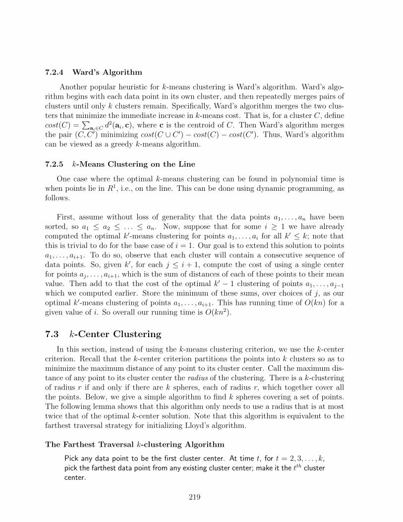
7.2.4 Ward’s Algorithm

Another popular heuristic for k-means clustering is Ward’s algorithm. Ward’s algo-rithm begins with each data point in its own cluster, and then repeatedly merges pairs ofclusters until only k clusters remain. Specifically, Ward’s algorithm merges the two clus-ters that minimize the immediate increase in k-means cost. That is, for a cluster C, definecost(C) =

∑ai∈C d

2(ai, c), where c is the centroid of C. Then Ward’s algorithm mergesthe pair (C,C ′) minimizing cost(C ∪ C ′) − cost(C) − cost(C ′). Thus, Ward’s algorithmcan be viewed as a greedy k-means algorithm.

7.2.5 k-Means Clustering on the Line

One case where the optimal k-means clustering can be found in polynomial time iswhen points lie in R1, i.e., on the line. This can be done using dynamic programming, asfollows.

First, assume without loss of generality that the data points a1, . . . , an have beensorted, so a1 ≤ a2 ≤ . . . ≤ an. Now, suppose that for some i ≥ 1 we have alreadycomputed the optimal k′-means clustering for points a1, . . . , ai for all k′ ≤ k; note thatthis is trivial to do for the base case of i = 1. Our goal is to extend this solution to pointsa1, . . . , ai+1. To do so, observe that each cluster will contain a consecutive sequence ofdata points. So, given k′, for each j ≤ i + 1, compute the cost of using a single centerfor points aj, . . . , ai+1, which is the sum of distances of each of these points to their meanvalue. Then add to that the cost of the optimal k′ − 1 clustering of points a1, . . . , aj−1

which we computed earlier. Store the minimum of these sums, over choices of j, as ouroptimal k′-means clustering of points a1, . . . , ai+1. This has running time of O(kn) for agiven value of i. So overall our running time is O(kn2).

7.3 k-Center Clustering

In this section, instead of using the k-means clustering criterion, we use the k-centercriterion. Recall that the k-center criterion partitions the points into k clusters so as tominimize the maximum distance of any point to its cluster center. Call the maximum dis-tance of any point to its cluster center the radius of the clustering. There is a k-clusteringof radius r if and only if there are k spheres, each of radius r, which together cover allthe points. Below, we give a simple algorithm to find k spheres covering a set of points.The following lemma shows that this algorithm only needs to use a radius that is at mosttwice that of the optimal k-center solution. Note that this algorithm is equivalent to thefarthest traversal strategy for initializing Lloyd’s algorithm.

The Farthest Traversal k-clustering Algorithm

Pick any data point to be the first cluster center. At time t, for t = 2, 3, . . . , k,pick the farthest data point from any existing cluster center; make it the tth clustercenter.

219

Theorem 7.3 If there is a k-clustering of radius r2, then the above algorithm finds a

k-clustering with radius at most r.

Proof: Suppose for contradiction that there is some data point x that is distance greaterthan r from all centers chosen. This means that each new center chosen was distancegreater than r from all previous centers, because we could always have chosen x. Thisimplies that we have k+1 data points, namely the centers chosen plus x, that are pairwisemore than distance r apart. Clearly, no two such points can belong to the same clusterin any k-clustering of radius r

2, contradicting the hypothesis.

7.4 Finding Low-Error Clusterings

In the previous sections we saw algorithms for finding a local optimum to the k-meansclustering objective, for finding a global optimum to the k-means objective on the line, andfor finding a factor 2 approximation to the k-center objective. But what about findinga clustering that is close to the correct answer, such as the true clustering of proteinsby function or a correct clustering of news articles by topic? For this we need someassumption about the data and what the correct answer looks like. The next few sectionsconsider algorithms based on different such assumptions.

7.5 Spectral Clustering

Let A be a n×d data matrix with each row a data point and suppose we want to partitionthe data points into k clusters. Spectral Clustering refers to a class of clustering algorithmswhich share the following outline:

• Find the space V spanned by the top k (right) singular vectors of A.

• Project data points into V .

• Cluster the projected points.

7.5.1 Why Project?

The reader may want to read Section 3.9.3, which shows the efficacy of spectral clusteringfor data stochastically generated from a mixture of spherical Gaussians. Here, we look atgeneral data which may not have a stochastic generation model.

We will later describe the last step in more detail. First, lets understand the centraladvantage of doing the projection to V . It is simply that for any reasonable (unknown)clustering of data points, the projection brings data points closer to their cluster centers.This statement sounds mysterious and likely false, since the assertion is for ANY rea-sonable unknown clustering. We quantify it in Theorem 7.4. First some notation: Werepresent a k-clustering by a n× d matrix C (same dimensions as A), where row i of C is

220

Figure 7.3: Clusters in the full space and their projections

the center of the cluster to which data point i belongs. So, there are only k distinct rowsof C and each other row is a copy of one of these rows. The k-means objective function,namely, the sum of squares of the distances of data points to their cluster centers is

n∑i=1

|ai − ci|2 = ||A− C||2F .

The projection reduces the sum of distance squares to cluster centers from ||A − C||2Fto at most 8k||A − C||22 in the projection. Recall that ||A − C||2 is the spectral norm,which is the top singular value of A − C. Now, ||A − C||2F =

∑t σ

2t (A) and often,

||A − C||F >>√k||A − C||2 and so the projection substantially reduces the sum of

squared distances to cluster centers.

We will see later that in many clustering problems, including models like mixtures ofGaussians and Stochastic Block Models of communities, there is a desired clustering Cwhere the regions overlap in the whole space, but are separated in the projection. Figure7.3 is a schematic illustration. Now we state the theorem and give its surprisingly simpleproof.

Theorem 7.4 Let A be an n × d matrix with Ak the projection of the rows of A to thesubspace of the first k right singular vectors of A. For any matrix C of rank less than orequal to k

||Ak − C||2F ≤ 8k||A− C||22.

221

Ak is a matrix that is close to every C, in the sense ||Ak−C||2F ≤ 8k||A−C||22. Whilethis seems contradictory, another way to state this is that for C far away from Ak inFrobenius norm, ||A− C||2 will also be high.

Proof: Since the rank of (Ak − C) is less than or equal to 2k,

||Ak − C||2F ≤ 2k||Ak − C||22 and

||Ak − C||2 ≤ ||Ak − A||2 + ||A− C||2 ≤ 2||A− C||2.

The last inequality follows since Ak is the best rank k approximation in spectral norm(Theorem 3.9) and C has rank at most k. The theorem follows.

Suppose now in the clustering C we would like to find, the cluster centers that are pairwiseat least Ω(

√k||A − C||2) apart. This holds for many clustering problems including data

generated by stochastic models. Then, it will be easy to see that in the projection,most data points are a constant factor farther from centers of other clusters than theirown cluster center and this makes it very easy for the following algorithm to find theclustering C modulo a small fraction of errors.

7.5.2 The Algorithm

Denote ||A−C||2/√n by σ(C). In the next section, we give an interpretation of ||A−C||2

indicating that σ(C) is akin to the standard deviation of clustering C and hence thenotation σ(C). We assume for now that σ(C) is known to us for the desired clustering C.This assumption can be removed by essentially doing a binary search.

Spectral Clustering - The Algorithm

1. Find the top k right singular vectors of data matrix A and project rows of A to thespace spanned by them to get Ak.(cf. Section 3.5).

2. Select a random row from Ak and form a cluster with all rows of Ak at distance lessthan 6kσ(C)/ε from it.

3. Repeat Step 2 k times.

Theorem 7.5 If in a k-clustering C, every pair of centers is separated by at least 15kσ(C)/εand every cluster has at least εn points in it, then with probability at least 1− ε, SpectralClustering finds a clustering C ′ that differs from C on at most ε2n points.

Proof: Let vi denote row i of Ak. We first show that for most data points, the projectionof data point is within distance 3kσ(C)/ε of its cluster center. I.e., we show that |M | issmall, where,

M = i : |vi − ci| ≥ 3kσ(C)/ε.

222

Now, ||Ak−C||2F =∑

i |vi−ci|2 ≥∑

i∈M |vi−ci|2 ≥ |M |9k2σ2(C)ε2

. So, using Theorem 7.4,we get:

|M |9k2σ2(C)

ε2≤ ||Ak − C||2F ≤ 8knσ2(C) =⇒ |M | ≤ 8ε2n

9k. (7.1)

Call a data point i “good” if i /∈ M . For any two good data points i and j belong-ing to the same cluster, since, their projections are within 3kσ(C)/ε of the center of thecluster, projections of the two data points are within 6kσ(C)/ε of each other. On theother hand, if two good data points i and k are in different clusters, since, the centersof the two clusters are at least 15kσ(C)/ε apart, their projections must be greater than15kσ(C)/ε− 6kσ(C)/ε = 9kσ(C)/ε apart. So, if we picked a good data point (say pointi) in Step 2, the set of good points we put in its cluster is exactly the set of good pointsin the same cluster as i. Thus, if in each of the k executions of Step 2, we picked a goodpoint, all good points are correctly clustered and since |M | ≤ ε2n, the theorem would hold.

To complete the proof, we must argue that the probability of any pick in Step 2 beingbad is small. The probability that the first pick in Step 2 is bad is at most |M |/n ≤ ε2/k.For each subsequent execution of Step 2, all the good points in at least one cluster areremaining candidates. So there are at least (ε−ε2)n good points left and so the probabilitythat we pick a bad point is at most |M |/(ε−ε2)n which is at most ε/k. The union boundover the k executions yields the desired result.

7.5.3 Means Separated by Ω(1) Standard Deviations

For probability distribution on the real line, the mnemonic “means separated by sixstandard deviations” suffices to distinguish different distributions. Spectral Clusteringenables us to do the same thing in higher dimensions provided k ∈ O(1) and six isreplaced by some constant. First we define standard deviation for general not necessarilystochastically generated data: it is just the maximum over all unit vectors v of the squareroot of the mean squared distance of data points from their cluster centers in the directionv, namely, the standard deviation σ(C) of clustering C is defined as:

σ(C)2 =1

nMaxv:|v|=1

n∑i=1

[(ai − ci) · v]2 =1

nMaxv:|v|=1|(A− C)v|2 =

1

n||A− C||22.

This coincides with the definition of σ(C) we made earlier. Assuming k ∈ O(1), it is easyto see that the Theorem 7.5 can be restated as

If cluster centers in C are separated by Ω(σ(C)), then the spectral clusteringalgorithm finds C ′ which differs from C only in a small fraction of data points.

It can be seen that the “means separated by Ω(1) standard deviations” condition holdsfor many stochastic models. We illustrate with two examples here. First, suppose we havea mixture of k ∈ O(1) spherical Gaussians, each with standard deviation one. The data

223

is generated according to this mixture. If the means of the Gaussians are Ω(1) apart,then the condition - means separated by Ω(1) standard deviations- is satisfied and so ifwe project to the SVD subspace and cluster, we will get (nearly) the correct clustering.This was already discussed in detail in Chapter ??.

We discuss a second example. Stochastic Block Models are models of communities.Suppose there are k communities C1, C2, . . . , Ck among a population of n people. Sup-pose the probability of two people in the same community knowing each other is p andif they are in different communities, the probability is q, where, q < p.33 We assume theevents that person i knows person j are independent across all i and j.

Specifically, we are given an n × n data matrix A, where aij = 1 if and only if i andj know each other. We assume the aij are independent random variables, and use ai todenote the ith row of A. It is useful to think of A as the adjacency matrix of a graph, suchas the friendship network in Facebook. We will also think of the rows ai as data points.The clustering problem is to classify the data points into the communities they belong to.In practice, the graph is fairly sparse, i.e., p and q are small, namely, O(1/n) or O(lnn/n).

Consider the simple case of two communities with n/2 people in each and with

p =α

nq =

β

nwhere α, β ∈ O(lnn).

Let u and v be the centroids of the data points in community one and community tworespectively; so ui ≈ p for i ∈ C1 and uj ≈ q for j ∈ C2 and vi ≈ q for i ∈ C1 and vj ≈ pfor j ∈ C2. We have

|u− v|2 =n∑j=1

(uj − vj)2 ≈ (α− β)2

n2n =

(α− β)2

n.

Inter-centroid distance ≈ α− β√n. (7.2)

We need to upper bound ||A − C||2. This is non-trivial since we have to prove auniform upper bound on |(A − C)v| for all unit vectors v. Fortunately, the subject toRandom Matrix Theory (RMT) already does this for us. RMT tells that

||A− C||2 ≤ O∗(√np) = O∗(

√α),

where, the O∗ hides logarithmic factors. So as long as α − β ∈ Ω∗(√α), we have the

means separated by Ω(1) standard deviations and spectral clustering works.

33More generally, for each pair of communities a and b, there could be a probability pab that a personfrom community a knows a person from community b. But for the discussion here, we take paa = p forall a and pab = q, for all a 6= b.

224

One important observation is that in these examples as well as many others, the k-means objective function in the whole space is too high and so the projection is essentialbefore we can cluster.

7.5.4 Laplacians

An important special case of spectral clustering is when k = 2 and a spectral algorithmis applied to the Laplacian matrix L of a graph, which is defined as

L = D − A

where A is the adjacency matrix and D is a diagonal matrix of degrees. Since A has anegative sign, we look at the lowest two singular values and corresponding vectors ratherthan the highest,

L is a symmetric matrix and is easily seen to be posiitve semi-definite: for any vectorx, we have

xTLx =∑i

diix2i −

∑(i,j)∈E

xixj =1

2

∑(i,j)∈E

(xi − xj)2.

Also since all row sums of L (and L is symmetric) are zero, its lowest eignvalue is 0 withthe eigenvector 1 of all 1’s. This is also the lowest singular vector of L. The projectionof all data points (rows) to this vector is just the origin and so gives no information. Ifwe take the second lowest singular vector and project to it which is essentially projectingto the space of the bottom two singular vectors, we get the very simple problem of n realnumbers which we need to cluster into two clusters.

7.5.5 Local spectral clustering

So far our emphasis has been on partitioning the data into disjoint clusters. However,the structure of many data sets consists of over lapping communities. In this case usingk-means with spectral clustering, the overlap of two communities shows up as a commu-nity. This is illustrated in Figure 7.4.

An alternative to using k-means with spectral clustering is to find the minimum 1-norm vector in the space spanned by the top singular vectors. Let A be the matrix whosecolumns are the singular vectors. To find a vector y in the space spanned by the columnsof A solve the linear system Ax = y. This is a slightly different looking problem thenAx = c where c is a constant vector. To convert Ax = y to the more usual form write it

as [A,−I]

(xy

)= 0. However, if we want to minimize ||y||1 the solution is x = y = 0.

Thus we add the row 1, 1, . . . 1, 0, 0, . . . 0 to [A,−I] and a 1 to the top of the vector [x, y]to force the coordinates of x to add up to one. Minimizing ||y||1 does not appear to be alinear program but we can write y = ya − yb and require ya ≥ 0 and yb ≥ 0. Now finding

225

the minimum one norm vector in the span of the columns of A is the linear program

min

(∑i

yai +∑i

ybi

)subject to (A,−I, I)

xyayb

= 0 ya ≥ 0 yb ≥ 0.

Local communitiesIn large social networks with a billion vertices, global clustering is likely to result incommunities of several hundred million vertices. What you may actually want is a localcommunity containing several individuals with only 50 vertices. To do this if one starts arandom walk at a vertex v and computes the frequency of visiting vertices, it will convergeto the first singular vector. However, the distribution after a small number of steps willbe primarily in the small community containing v and will be proportional to the firstsingular vector distribution restricted to the vertices in the small community containing v,only will be higher by some constant value. If one wants to determine the local communi-ties containing vertices v1, v2, and v3, start with three probability distributions, one withprobability one at v1, one with probability one at v2, and one with probability one at v3

and find early approximation to the first three singular vectors. Then find the minimum1-norm vector in the space spanned by the early approximations.

Hidden structureIn the previous section we discussed overlapping communities. Another issue is hiddenstructure. Suppose the vertices of a social network could be partitioned into a number ofstrongly connected communities. By strongly connected we mean the probability of anedge between two vertices in a community is much higher than the probability of an edgebetween two vertices in different communities. Suppose the vertices of the graph couldbe partitioned in another way which was incoherent34 with the first partitioning and theprobability of an edge between two vertices in one of these communities is higher than anedge between two vertices in different communities. If the probability of an edge betweentwo vertices in a community of this second partitioning is less than that in the first, thena clustering algorithm is likely to find the first partitioning rather than the second. How-ever, the second partitioning, which we refer to as hidden structure, may be the structurethat we want to find. The way to do this is to use your favorite clustering algorithm toproduce the dominant structure and then stochastically weaken the dominant structureby removing some community edges in the graph. Now if you apply the clustering algo-rithm to the modified graph, it can find the hidden community structure. Having donethis, go back to the original graph, weaken the hidden structure and reapply the cluster-ing algorithm. It will now find a better approximation to the dominant structure. Thistechnology can be used to find a number of hidden levels in several types of social networks.

34incoherent, give definition

226

1 1 1 1 1 1 0 0 01 1 1 1 1 1 0 0 01 1 1 1 1 1 0 0 01 1 1 1 1 1 0 0 01 1 1 1 1 1 1 1 11 1 1 1 1 1 1 1 10 0 0 0 1 1 0 0 00 0 0 0 1 1 0 0 00 0 0 0 1 1 0 0 0

0.33 0.310.33 0.310.33 0.310.33 0.310.44 −0.090.44 −0.090.24 −0.490.24 −0.490.24 −0.49

(a) (b) (c);

Figure 7.4: (a) illustrates the adjacency matrix of a graph with a six vertex clique thatoverlaps a five vertex clique in two vertices. (b) illustrates the matrix where columnsconsist of the top two singular vectors, and (c) illustrates the mapping of rows in thesingular vector matrix to three points in two dimensional space. Instead of two cliqueswe get the non-overlapping portion of each of the two clique plus their intersection ascommunities instead of the two cliques as communities.

Block modelOne technique for generating graphs with communities is to use the block model wherethe vertices are partitioned into blocks and each block is a GNP graph generated withsome edge probability. The edges in off diagonal blocks are generated with a lower prob-ability. One can also generate graphs with hidden structure. For example, the vertices inan n vertex graph might be partitioned into two communities, the first community havingvertices 1 to n/2 and the second community having vertices n/2 + 1 to n. The dominantstructure is generated with probability p1 for edges within communities and probability q1

for edges between communities. The the vertices are randomly permuted and the hiddenstructure is generated using the first n/2 vertices in the permuted order for one commu-nity and the remaining vertices for the second community with probabilities p2 and q2

which ar lower than p1 and q1..

An interesting question is how to determine the quality of a community found. Manyresearchers use an existing standard of what the communities are. However, if you wantto using clustering techniques to find communities there probably is no external standardor you would just use that instead of clustering. A way to determine if you have found areal community structure is to ask if the graph is more likely generated by a model of thestructure found than by a completely random model. Suppose you found a partition oftwo communities each with n/2 vertices. Using the number of edges in each communityand the number of inter community edges ask what is the probability of the graph beinggenerated by a bloc model where p and q are the probabilities determined by the edgedensity within communities and the edge density between communities. One can comparethis probability with the probability that the graph was generated by a GNP model withprobability (p+ q)/2.

227

7.6 Approximation Stability

7.6.1 The Conceptual Idea

We now consider another condition that will allow us to produce accurate clustersfrom data. To think about this condition, imagine that we are given a few thousand newsarticles that we want to cluster by topic. These articles could be represented as points ina high-dimensional space (e.g., axes could correspond to different meaningful words, withcoordinate i indicating the frequency of that word in a given article). Or, alternatively, itcould be that we have developed some text-processing program that given two articles xand y computes some measure of distance d(x, y) between them. We assume there existssome correct clustering CT of our news articles into k topics; of course, we do not knowwhat CT is, that is what we want our algorithm to find.

If we are clustering with an algorithm that aims to minimize the k-means score of itssolution, then implicitly this means we believe that the clustering COPTkmeans of minimum k-means score is either equal to, or very similar to, the clustering CT . Unfortunately, findingthe clustering of minimum k-means score is NP-hard. So, let us broaden our belief a bitand assume that any clustering C whose k-means score is within 10% of the minimumis also very similar to CT . This should give us a little bit more slack. Unfortunately,finding a clustering of score within 10% of the minimum is also an NP-hard problem.Nonetheless, we will be able to use this assumption to efficiently find a clustering that isclose to CT . The trick is that NP-hardness is a worst-case notion, whereas in contrast,this assumption implies structure on our data.In particular, it implies that all clusteringsthat have score within 10% of the minimum have to be similar to each other. We willthen be able to utilize this structure in a natural “ball-growing” clustering algorithm.

7.6.2 Making this Formal

To make this discussion formal, we first specify what we mean when we say that twodifferent ways of clustering some data are “similar” to each other. Let C = C1, . . . , Ckand C ′ = C ′1, . . . , C ′k be two different k-clusterings of some dataset A. For example, Ccould be the clustering that our algorithm produces, and C ′ could be the clustering CT .Let us define the distance between these two clusterings to be the fraction of points thatwould have to be re-clustered in C to make C match C ′, where by “match” we mean thatthere should be a bijection between the clusters of C and the clusters of C ′. We can writethis distance mathematically as:

dist(C, C ′) = minσ

1

n

k∑i=1

|Ci \ C ′σ(i)|,

where the minimum is over all permutations σ of 1, . . . , k.

For c > 1 and ε > 0 we say that a data set satisfies (c, ε)-approximation-stabilitywith respect to a given objective (such as k-means or k-median) if every clustering C

228

whose cost is within a factor c of the minimum-cost clustering for that objective satisfiesdist(C, CT ) < ε. That is, it is sufficient to be within a factor c of optimal to the ourobjective in order for the fraction of points clustered incorrectly to be less than ε. We willspecifically focus in this discussion on the k-median objective rather than the k-meansobjective, since it is a bit easier to work with.

What we will now show is that under this condition, even though it may be NP-hardin general to find a clustering that is within a factor c of optimal, we can nonethelessefficiently find a clustering C ′ such that dist(C ′, CT ) ≤ ε, so long as all clusters in CT arereasonably large. To simplify notation, let C∗ denote the clustering of minimum k-mediancost, and to keep the discussion simpler, let us also assume that CT = C∗; that is, thetarget clustering is also the clustering with the minimum k-median score.

7.6.3 Algorithm and Analysis

Before presenting an algorithm, we begin with a helpful lemma that will guide ourdesign. For a given data point ai, define its weight w(ai) to be its distance to the centerof its cluster in C∗. Notice that the k-median cost of C∗ is OPT =

∑ni=1w(ai). Define

wavg = OPT/n to be the average weight of the points in A. Finally, define w2(ai) to bethe distance of ai to its second-closest center in C∗.

Lemma 7.6 Assume dataset A satisfies (c, ε) approximation-stability with respect to thek-median objective, each cluster in CT has size at least 2εn, and CT = C∗. Then,

1. Fewer than εn points ai have w2(ai)− w(ai) ≤ (c− 1)wavg/ε.

2. At most 5εn/(c− 1) points ai have w(ai) ≥ (c− 1)wavg/(5ε).

Proof: For part (1), suppose that εn points ai have w2(ai) − w(ai) ≤ (c − 1)wavg/ε.Consider modifying CT to a new clustering C ′ by moving each of these points ai intothe cluster containing its second-closest center. By assumption, the k-means cost of theclustering has increased by at most εn(c − 1)wavg/ε = (c − 1) · OPT. This means thatthe cost of the new clustering is at most cOPT . However, dist(C ′, CT ) = ε because (a) wemoved εn points to different clusters, and (b) each cluster in CT has size at least 2εn so theoptimal permutation σ in the definition of dist remains the identity. So, this contradictsapproximation stability. Part (2) follows from the definition of “average”; if it did nothold then

∑ni=1w(ai) > nwavg, a contradiction.

A datapoint ai is bad if it satisfies either item (1) or (2) of Lemma 7.6 and good if itsatisfies neither one. So, there are at most b = εn+ 5εn

c−1bad points and the rest are good.

Define “critical distance” dcrit = (c−1)wavg5ε

. Lemma 7.6 implies that the good points havedistance at most dcrit to the center of their own cluster in C∗ and distance at least 5dcritto the center of any other cluster in C∗.

229

This suggests the following algorithm. Suppose we create a graph G with the pointsai as vertices, and edges between any two points ai and aj with d(ai, aj) < 2dcrit. Noticethat by triangle inequality, the good points within the same cluster in C∗ have distanceless than 2dcrit from each other so they will be fully connected and form a clique. Also,again by triangle inequality, any edge that goes between different clusters must be be-tween two bad points. In particular, if ai is a good point in one cluster, and it has an edgeto some other point aj, then aj must have distance less than 3dcrit to the center of ai’scluster. This means that if aj had a different closest center, which obviously would alsobe at distance less than 3dcrit, then ai would have distance less than 2dcrit+3dcrit = 5dcritto that center, violating its goodness. So, bridges in G between different clusters can onlyoccur between bad points.

Assume now that each cluster in CT has size at least 2b+1; this is the sense in which weare requiring that εn be small compared to the smallest cluster in CT . In this case, createa new graph H by connecting any two points ai and aj that share at least b+ 1 neighborsin common in G, themselves included. Since every cluster has at least 2b+ 1− b = b+ 1good points, and these points are fully connected in G, this means that H will contain anedge between every pair of good points in the same cluster. On the other hand, since theonly edges in G between different clusters are between bad points, and there are at mostb bad points, this means that H will not have any edges between different clusters in CT .Thus, if we take the k largest connected components in H, these will all correspond tosubsets of different clusters in CT , with at most b points remaining.

At this point we have a correct clustering of all but at most b points in A. Call theseclusters C1, . . . , Ck, where Cj ⊆ C∗j . To cluster the remaining points ai, we assign themto the cluster Cj that minimizes the median distance between ai and points in Cj. Sinceeach Cj has more good points than bad points, and each good point in Cj has distance atmost dcrit to center c∗j , by triangle inequality the median of these distances must lie in therange [d(ai, c∗i ) − dcrit, d(ai, c

∗i ) + dcrit]. This means that this second step will correctly

cluster all points ai for which w2(ai)− w(ai) > 2dcrit. In particular, we correctly clusterall points except possibly for some of the at most εn satisfying item (1) of Lemma 7.6.

The above discussion assumes the value dcrit is known to our algorithm; we leave it asan exercise to the reader to modify the algorithm to remove this assumption. Summariz-ing, we have the following algorithm and theorem.

Algorithm k-Median Stability (given c, ε, dcrit)

1. Create a graph G with a vertex for each datapoint in A, and an edge betweenvertices i and j if d(ai, aj) ≤ 2dcrit.

2. Create a graph H with a vertex for each vertex in G and an edge between vertices iand j if i and j share at least b+ 1 neighbors in common, themselves included, forb = εn+ 5εn

c−1. Let C1, . . . , Ck denote the k largest connected components in H.

230

3. Assign each point not in C1∪ . . .∪Ck to the cluster Cj of smallest median distance.

Theorem 7.7 Assume A satisfies (c, ε) approximation-stability with respect to the k-median objective, that each cluster in CT has size at least 10ε

c−1n+2εn+1, and that CT = C∗.

Then Algorithm k-Median Stability will find a clustering C such that dist(C, CT ) ≤ ε.

7.7 High-Density Clusters

We now turn from the assumption that clusters are center-based to the assumptionthat clusters consist of high-density regions, separated by low-density moats such as inFigure 7.1.

7.7.1 Single Linkage

One natural algorithm for clustering under the high-density assumption is called singlelinkage. This algorithm begins with each point in its own cluster and then repeatedlymerges the two “closest” clusters into one, where the distance between two clusters isdefined as the minimum distance between points in each cluster. That is, dmin(C,C ′) =minx∈C,y∈C′ d(x,y), and the algorithm merges the two clusters C and C ′ whose dmin valueis smallest over all pairs of clusters breaking ties arbitrarily. It then continues until thereare only k clusters. This is called an agglomerative clustering algorithm because it beginswith many clusters and then starts merging, or agglomerating them together.35 Single-linkage is equivalent to running Kruskal’s minimum-spanning-tree algorithm, but haltingwhen there are k trees remaining. The following theorem is fairly immediate.

Theorem 7.8 Suppose the desired clustering C∗1 , . . . , C∗k satisfies the property that there

exists some distance σ such that

1. any two data points in different clusters have distance at least σ, and

2. for any cluster C∗i and any partition of C∗i into two non-empty sets A and C∗i \ A,there exist points on each side of the partition of distance less than σ.

Then, single-linkage will correctly recover the clustering C∗1 , . . . , C∗k .

Proof: Consider running the algorithm until all pairs of clusters C and C ′ have dmin(C,C ′) ≥ σ.At that point, by (2), each target cluster C∗i will be fully contained within some clusterof the single-linkage algorithm. On the other hand, by (1) and by induction, each clusterC of the single-linkage algorithm will be fully contained within some C∗i of the targetclustering, since any merger of subsets of distinct target clusters would require dmin ≥ σ.Therefore, the single-linkage clusters are indeed the target clusters.

35Other agglomerative algorithms include complete linkage which merges the two clusters whose max-imum distance between points is smallest, and Ward’s algorithm described earlier that merges the twoclusters that cause the k-means cost to increase by the least.

231

7.7.2 Robust Linkage

The single-linkage algorithm is fairly brittle. A few points bridging the gap betweentwo different clusters can cause it to do the wrong thing. As a result, there has beensignificant work developing more robust versions of the algorithm.

One commonly used robust version of single linkage is Wishart’s algorithm. A ballof radius r is created for each point with the point as center. The radius r is graduallyincreased starting from r = 0. The algorithm has a parameter t. When a ball has t ormore points the center point becomes active. When two balls with active centers intersectthe two center points are connected by an edge. The parameter t prevents a thin stringof points between two clusters from causing a spurious merger. Note that Wishart’s al-gorithm with t = 1 is the same as single linkage.

In fact, if one slightly modifies the algorithm to define a point to be live if its ballof radius r/2 contains at least t points, then it is known [CD10] that a value of t =O(d log n) is sufficient to recover a nearly correct solution under a natural distributionalformulation of the clustering problem. Specifically, suppose data points are drawn fromsome probability distribution D over Rd, and that the clusters correspond to high-densityregions surrounded by lower-density moats. More specifically, the assumption is that

1. for some distance σ > 0, the σ-interior of each target cluster C∗i has density at leastsome quantity λ (the σ-interior is the set of all points at distance at least σ fromthe boundary of the cluster),

2. the region between target clusters has density less than λ(1− ε) for some ε > 0,

3. the clusters should be separated by distance greater than 2σ, and

4. the σ-interior of the clusters contains most of their probability mass.

Then, for sufficiently large n, the algorithm will with high probability find nearly correctclusters. In this formulation, we allow points in low-density regions that are not in anytarget clusters at all. For details, see [CD10].

Robust Median Neighborhood Linkage robustifies single linkage in a different way.This algorithm guarantees that if it is possible to delete a small fraction of the data suchthat for all remaining points x, most of their |C∗(x)| nearest neighbors indeed belong totheir own cluster C∗(x), then the hierarchy on clusters produced by the algorithm willinclude a close approximation to the true clustering. We refer the reader to [BLG14] forthe algorithm and proof.

7.8 Kernel Methods

Kernel methods combine aspects of both center-based and density-based clustering.In center-based approaches like k-means or k-center, once the cluster centers are fixed, the

232

Voronoi diagram of the cluster centers determines which cluster each data point belongsto. This implies that clusters are pairwise linearly separable.

If we believe that the true desired clusters may not be linearly separable, and yet wewish to use a center-based method, then one approach, as in the chapter on learning,is to use a kernel. Recall that a kernel function K(x,y) can be viewed as performingan implicit mapping φ of the data into a possibly much higher dimensional space, andthen taking a dot-product in that space. That is, K(x,y) = φ(x) · φ(y). This is thenviewed as the affinity between points x and y. We can extract distances in this newspace using the equation |z1 − z2|2 = z1 · z1 + z2 · z2 − 2z1 · z2, so in particular we have|φ(x)−φ(y)|2 = K(x,x)+K(y,y)−2K(x,y). We can then run a center-based clusteringalgorithm on these new distances.

One popular kernel function to use is the Gaussian kernel. The Gaussian kernel usesan affinity measure that emphasizes closeness of points and drops off exponentially as thepoints get farther apart. Specifically, we define the affinity between points x and y by

K(x,y) = e−1

2σ2‖x−y‖2 .

Another way to use affinities is to put them in an affinity matrix, or weighted graph.This graph can then be separated into clusters using a graph partitioning procedure suchas the one in following section.

7.9 Recursive Clustering Based on Sparse Cuts

We now consider the case that data are nodes in an undirected connected graphG(V,E) where an edge indicates that the end point vertices are similar. Recursive clus-tering starts with all vertices in one cluster and recursively splits a cluster into two partswhenever there is a small number of edges from one part to the other part of the cluster.Formally, for two disjoint sets S and T of vertices, define

Φ(S, T ) =Number of edges from S to T

Total number of edges incident to S in G.

Φ(S, T ) measures the relative strength of similarities between S and T . Let d(i) be thedegree of vertex i and for a subset S of vertices, let d(S) =

∑i∈S d(i). Let m be the total

number of edges in the graph. The following algorithm aims to cut only a small fractionof the edges and to produce clusters that are internally consistent in that no subset of thecluster has low similarity to the rest of the cluster.

Recursive Clustering: Select an appropriate value for ε. If a current clusterW has a subset S with d(S) ≤ 1

2d(W ) and Φ(S, S ⊆ W ) ≤ ε, then split W

into two clusters S and W \ S. Repeat until no such split is possible.

Theorem 7.9 At termination of Recursive Clustering, the total number of edges betweenvertices in different clusters is at most O(εm lnn).

233

Proof: Each edge between two different clusters at the end was deleted at some stageby the algorithm. We will “charge” edge deletes to vertices and bound the total charge.When the algorithm partitions a cluster W into S and W \S with d(S) ≤ (1/2)d(W ), each

k ∈ S is charged d(k)d(W )

times the number of edges being deleted. Since Φ(S,W \ S) ≤ ε,

the charge added to each k ∈ W is a most εd(k). A vertex is charged only when it isin the smaller part, d(S) ≤ d(W )/2, of the cut. So between any two times it is charged,d(W ) is reduced by a factor of at least two and so a vertex can be charged at mostlog2m ≤ O(lnn) times, proving the theorem.

Implementing the algorithm requires computing MinS⊆WΦ(S,W \S) which is an NP-hard problem. So the theorem cannot be implemented right away. Luckily, eigenvalues andeigenvectors, which can be computed fast, give an approximate answer. The connectionbetween eigenvalues and sparsity, known as Cheeger’s inequality, is deep with applicationsto Markov chains among others. We do not discuss this here.

7.10 Dense Submatrices and Communities

Represent n data points in d-space by the rows of an n× d matrix A. Assume that Ahas all non-negative entries. Examples to keep in mind for this section are the document-term matrix and the customer-product matrix. We address the question of how to defineand find efficiently a coherent large subset of rows. To this end, the matrix A can berepresented by a bipartite graph Figure 7.5. One side has a vertex for each row and theother side a vertex for each column. Between the vertex for row i and the vertex forcolumn j, there is an edge with weight aij.

We want a subset S of row vertices and a subset T of column vertices so that

A(S, T ) =∑

i∈S,j∈T

aij

is high. This simple definition is not good since A(S, T ) will be maximized by takingall rows and columns. We need a balancing criterion that ensures that A(S, T ) is high

relative to the sizes of S and T . One possibility is to maximize A(S,T )|S||T | . This is not a good

measure either, since it is maximized by the single edge of highest weight. The definitionwe use is the following. Let A be a matrix with non-negative entries. For a subset S ofrows and a subset T of columns, the density d(S, T ) of S and T is d(S, T ) = A(S,T )√

|S||T |. The

density d(A) of A is defined as the maximum value of d(S, T ) over all subsets of rows andcolumns. This definition applies to bipartite as well as non-bipartite graphs.

One important case is when A’s rows and columns both represent the same set andaij is the similarity between object i and object j. Here d(S, S) = A(S,S)

|S| . If A is an n× n0-1 matrix, it can be thought of as the adjacency matrix of an undirected graph, andd(S, S) is the average degree of a vertex in S. The subgraph of maximum average degreein a graph can be found exactly by network flow techniques, as we will show in the next

234

Figure 7.5: Example of a bipartite graph.

section. We do not know an efficient (polynomial-time) algorithm for finding d(A) exactlyin general. However, we show that d(A) is within a O(log2 n) factor of the top singularvalue of A assuming |aij| ≤ 1 for all i and j. This is a theoretical result. The gap may bemuch less than O(log2 n) for many problems, making singular values and singular vectorsquite useful. Also, S and T with d(S, T ) ≥ Ω(d(A)/ log2 n) can be found algorithmically.

Theorem 7.10 Let A be an n× d matrix with entries between 0 and 1. Then

σ1(A) ≥ d(A) ≥ σ1(A)

4 log n log d.

Furthermore, subsets S and T satisfying d(S, T ) ≥ σ1(A)4 logn log d

may be found from the topsingular vector of A.

Proof: Let S and T be the subsets of rows and columns that achieve d(A) = d(S, T ).Consider an n-vector u that is 1√

|S|on S and 0 elsewhere and a d-vector v that is 1√

|T |on T and 0 elsewhere. Then,

σ1 (A) ≥ uTAv =∑ij

uivjaij = d(S, T ) = d(A)

establishing the first inequality.

To prove the second inequality, express σ1 (A) in terms of the first left and rightsingular vectors x and y.

σ1(A) = xTAy =∑i,j

xiaijyj, |x| = |y| = 1.

Since the entries of A are non-negative, the components of the first left and right singularvectors must all be non-negative, that is, xi ≥ 0 and yj ≥ 0 for all i and j. To bound∑i,j

xiaijyj, break the summation into O (log n log d) parts. Each part corresponds to a

given α and β and consists of all i such that α ≤ xi < 2α and all j such that β ≤ yi < 2β.The log n log d parts are defined by breaking the rows into log n blocks with α equal to12

1√n, 1√

n, 2 1√

n, 4 1√

n, . . . , 1 and by breaking the columns into log d blocks with β equal

235

to 12

1√d, 1√

d, 2√

d, 4√

d, . . . , 1. The i such that xi <

12√n

and the j such that yj <1

2√d

will

be ignored at a loss of at most 14σ1(A). Exercise 7.27 proves the loss is at most this amount.

Since∑i

x2i = 1, the set S = i|α ≤ xi < 2α has |S| ≤ 1

α2 and similarly,

T = j|β ≤ yj ≤ 2β has |T | ≤ 1β2 . Thus∑

iα≤xi≤2α

∑j

β≤yj≤2β

xiyjaij ≤ 4αβA(S, T )

≤ 4αβd(S, T )√|S||T |

≤ 4d(S, T )

≤ 4d(A).

From this it follows thatσ1 (A) ≤ 4d (A) log n log d

ord (A) ≥ σ1(A)

4 logn log d

proving the second inequality.

It is clear that for each of the values of (α, β), we can compute A(S, T ) and d(S, T )as above and taking the best of these d(S, T ) ’s gives us an algorithm as claimed in thetheorem.

Note that in many cases, the non-zero values of xi and yj after zeroing out the lowentries will only go from 1

21√n

to c√n

for xi and 12

1√d

to c√d

for yj, since the singular vectorsare likely to be balanced given that aij are all between 0 and 1. In this case, there willbe O(1) groups only and the log factors disappear.

Another measure of density is based on similarities. Recall that the similarity betweenobjects represented by vectors (rows of A) is defined by their dot products. Thus, simi-larities are entries of the matrix AAT . Define the average cohesion f(S) of a set S of rowsof A to be the sum of all pairwise dot products of rows in S divided by |S|. The averagecohesion of A is the maximum over all subsets of rows of the average cohesion of the subset.

Since the singular values of AAT are squares of singular values of A, we expect f(A)to be related to σ1(A)2 and d(A)2. Indeed it is. We state the following without proof.

Lemma 7.11 d(A)2 ≤ f(A) ≤ d(A) log n. Also, σ1(A)2 ≥ f(A) ≥ cσ1(A)2

logn.

f(A) can be found exactly using flow techniques as we will see later.

236

7.11 Community Finding and Graph Partitioning

Assume that data are nodes in a possibly weighted graph where edges represent somenotion of affinity between their endpoints. In particular, let G = (V,E) be a weightedgraph. Given two sets of nodes S and T , define

E(S, T ) =∑i∈Sj∈T

eij.

We then define the density of a set S to be

d(S, S) =E(S, S)

|S|.

If G is an undirected graph, then d(S, S) can be viewed as the average degree in thevertex-induced subgraph over S. The set S of maximum density is therefore the subgraphof maximum average degree. Finding such a set can be viewed as finding a tight-knitcommunity inside some network. In the next section, we describe an algorithm for findingsuch a set using network flow techniques.

Flow Methods Here we consider dense induced subgraphs of a graph. Aninduced subgraph of a graph consisting of a subset of the vertices of the graph along withall edges of the graph that connect pairs of vertices in the subset of vertices. We showthat finding an induced subgraph with maximum average degree can be done by networkflow techniques. This is simply maximizing the density d(S, S) over all subsets S of thegraph. First consider the problem of finding a subset of vertices such that the inducedsubgraph has average degree at least λ for some parameter λ. Then do a binary searchon the value of λ until the maximum λ for which there exists a subgraph with averagedegree at least λ is found.

Given a graph G in which one wants to find a dense subgraph, construct a directedgraph H from the given graph and then carry out a flow computation on H. H has anode for each edge of the original graph, a node for each vertex of the original graph,plus two additional nodes s and t. There is a directed edge with capacity one from s toeach node corresponding to an edge of the original graph and a directed edge with infinitecapacity from each node corresponding to an edge of the original graph to the two nodescorresponding to the vertices the edge connects. Finally, there is a directed edge withcapacity λ from each node corresponding to a vertex of the original graph to t.

Notice there are three types of cut sets of the directed graph that have finite capacity,Figure 7.6. The first cuts all arcs from the source. It has capacity e, the number of edgesof the original graph. The second cuts all edges into the sink. It has capacity λv, where vis the number of vertices of the original graph. The third cuts some arcs from s and somearcs into t. It partitions the set of vertices and the set of edges of the original graph intotwo blocks. The first block contains the source node s, a subset of the edges es, and a

237

s

[u,v]

[v,w]

[w,x]

u

v

w

x

t

1

1

1

∞∞

∞

∞∞∞

λ

λ

λ

λ

edges

vertices

Figure 7.6: The directed graph H used by the flow technique to find a dense subgraph

subset of the vertices vs defined by the subset of edges. The first block must contain bothend points of each edge in es; otherwise an infinite arc will be in the cut. The second blockcontains t and the remaining edges and vertices. The edges in this second block eitherconnect vertices in the second block or have one endpoint in each block. The cut set willcut some infinite arcs from edges not in es coming into vertices in vs. However, thesearcs are directed from nodes in the block containing t to nodes in the block containing s.Note that any finite capacity cut that leaves an edge node connected to s must cut thetwo related vertex nodes from t, Figure 7.6. Thus, there is a cut of capacity e− es + λvswhere vs and es are the vertices and edges of a subgraph. For this cut to be the minimalcut, the quantity e− es + λvs must be minimal over all subsets of vertices of the originalgraph and the capcity must be less than e and also less than λv.

If there is a subgraph with vs vertices and es edges where the ratio esvs

is sufficientlylarge so that eS

vS> e

v, then for λ such that eS

vS> λ > e

v, es − λvs > 0 and e− es + λvs < e.

Similarly e < λv and thus e− es + λvs < λv. This implies that the cut e− es + λvs is lessthan either e or λv and the flow algorithm will find a non-trivial cut and hence a propersubset. For different values of λ in the above range there maybe different non-trivial cuts.

Note that for a given density of edges, the number of edges grows as the square of thenumber of vertices and es

vsis less likely to exceed e

vif vS is small. Thus, the flow method

works well in finding large subsets since it works with eSvS

. To find small communities onewould need to use a method that worked with eS

v2Sas the following example illustrates.

Example: Consider finding a dense subgraph of 1,000 vertices and 2,000 internal edges ina graph of 106 vertices and 6×106 edges. For concreteness, assume the graph was generatedby the following process. First, a 1,000-vertex graph with 2,000 edges was generated as a

238

s t

edges and verticesin the community

1

cut

λ

∞

∞

∞

Figure 7.7: Cut in flow graph

random regular degree four graph. The 1,000-vertex graph was then augmented to have106 vertices and edges were added at random until all vertices were of degree 12. Notethat each vertex among the first 1,000 has four edges to other vertices among the first1,000 and eight edges to other vertices. The graph on the 1,000 vertices is much denserthan the whole graph in some sense. Although the subgraph induced by the 1,000 verticeshas four edges per vertex and the full graph has twelve edges per vertex, the probabilityof two vertices of the 1,000 being connected by an edge is much higher than for the graphas a whole. The probability is given by the ratio of the actual number of edges connectingvertices among the 1,000 to the number of possible edges if the vertices formed a completegraph.

p =e((v2

)) =2e

v(v − 1)

For the 1,000 vertices, this number is p = 2×2,0001,000×999

∼= 4× 10−3. For the entire graph this

number is p = 2×6×106

106×106= 12 × 10−6. This difference in probability of two vertices being

connected should allow us to find the dense subgraph.

In our example, the cut of all arcs out of s is of capacity 6 × 106, the total numberof edges in the graph, and the cut of all arcs into t is of capacity λ times the numberof vertices or λ × 106. A cut separating the 1,000 vertices and 2,000 edges would havecapacity 6× 106− 2, 000 + λ× 1, 000. This cut cannot be the minimum cut for any valueof λ since es

vs= 2 and e

v= 6, hence es

vs< e

v. The point is that to find the 1,000 vertices, we

have to maximize A(S, S)/|S|2 rather than A(S, S)/|S|. Note that A(S, S)/|S|2 penalizeslarge |S| much more and therefore can find the 1,000 node “dense” subgraph.

239

A =

1 1 1 0 01 1 1 0 01 1 1 0 00 0 0 1 10 0 0 1 1

V =

1 01 01 00 10 1

Figure 7.8: Illustration of spectral clustering.

7.12 Spectral Clustering Applied to Social Networks

Finding communities in social networks is different from other clustering for severalreasons. First we often want to find communities of size say 20 to 50 in networks with100 million vertices. Second a person is in a number of overlapping communities and thuswe are not finding disjoint clusters. Third there often are a number of levels of structureand a set of dominant communities may be hiding a set of weaker communities that areof interest. Spectral clustering is one approach to these issues.

In spectral clustering of the vertices of a graph, one creates a matrix V whose columnscorrespond to the first k singular vectors of the adjacency matrix. Each row of V isthe projection of a row of the adjacency matrix to the space spanned by the k singularvectors. In the example below, the graph has five vertices divided into two cliques, oneconsisting of the first three vertices and the other the last two vertices. The top two rightsingular vectors of the adjacency matrix, not normalized to length one, are (1, 1, 1, 0, 0)T

and (0, 0, 0, 1, 1)T . The five rows of the adjacency matrix projected to these vectors formthe 5 × 2 matrix in Figure 7.8. Here, there are two ideal clusters with all edges inside acluster being present including self-loops and all edges between clusters being absent. Thefive rows project to just two points, depending on which cluster the rows are in. If theclusters were not so ideal and instead of the graph consisting of two disconnected cliques,the graph consisted of two dense subsets of vertices where the two sets were connected byonly a few edges, then the singular vectors would not be indicator vectors for the clustersbut close to indicator vectors. The rows would be mapped to two clusters of points insteadof two points. A k-means clustering algorithm would find the clusters.

If the clusters were overlapping, then instead of two clusters of points, there would bethree clusters of points where the third cluster corresponds to the overlapping vertices ofthe two clusters. Instead of using k-means clustering, we might instead find the minimum1-norm vector in the space spanned by the two singular vectors. The minimum 1-normvector will not be an indicator vector, so we would threshold its values to create anindicator vector for a cluster. Instead of finding the minimum 1-norm vector in the spacespanned by the singular vectors in V, we might look for a small 1-norm vector close tothe subspace.

minx

(1− |x|1 + α cos(θ))

240

Here θ is the cosine of the angle between x and the space spanned by the two singularvectors. α is a control parameter that determines how close we want the vector to be tothe subspace. When α is large, x must be close to the subspace. When α is zero, x canbe anywhere.

Finding the minimum 1-norm vector in the space spanned by a set of vectors can beformulated as a linear programming problem. To find the minimum 1-norm vector in V,write V x = y where we want to solve for both x and y. Note that the format is differentfrom the usual format for a set of linear equations Ax = b where b is a known vector.

Finding the minimum 1-norm vector looks like a non-linear problem.

min |y|1 subject to V x = y

To remove the absolute value sign, write y = y1−y2 with y1 ≥ 0 and y2 ≥ 0. Then solve

min

(n∑i=1

y1i +n∑i=1

y2i

)subject to V x = y, y1 ≥ 0, and y2 ≥ 0.

Write V x = y1 − y2 as V x− y1 + y2 = 0. then we have the linear equations in a formatwe are accustomed to.

[V,−I, I]

xy1

y2

=

00...0

This is a linear programming problem. The solution, however, happens to be x = 0,y1 = 0, and y2 = 0. To resolve this, add the equation y1i = 1 to get a community con-taining the vertex i.

Often we are looking for communities of 50 or 100 vertices in graphs with hundreds ofmillion of vertices. We want a method to find such communities in time proportional tothe size of the community and not the size of the entire graph. Here spectral clusteringcan be used but instead of calculating singular vectors of the entire graph, we do some-thing else. Consider a random walk on a graph. If we walk long enough the probabilitydistribution converges to the first eigenvector. However, if we take only a few steps from astart vertex or small group of vertices that we believe define a cluster, the probability willdistribute over the cluster with some of the probability leaking out to the remainder ofthe graph. To get the early convergence of several vectors that ultimately converge to thefirst few singular vectors, take a subspace [x, Ax, A2x, A3x] and propagate the subspace.At each iteration find an orthonormal basis and then multiply each basis vector by A.Then take the resulting basis vectors after a few steps, say five, and find a minimum1-norm vector in the subspace.

241

A third issue that arises is when a dominant structure hides an important weakerstructure. One can run their algorithm to find the dominant structure and then weaken thedominant structure by randomly removing edges in the clusters so that the edge density issimilar to the remainder of the network. Then reapplying the algorithm often will uncoverweaker structure. Real networks often have several levels of structure. The techniquecan also be used to improve state of the art clustering algorithms. After weakening thedominant structure to find the weaker hidden structure one can go back to the original dataand weaken the hidden structure and reapply the algorithm to again find the dominantstructure. This improves most state of the art clustering algorithms.

242

7.13 Bibliographic Notes

Clustering has a long history. For a good general survey, see [Jai10]. For a collectionof surveys giving an in-depth treatment of many different approaches to, applications of,and perspectives on clustering, see [HMMR15]; e.g., see [AB15] for a good discussion ofcenter-based clustering. Lloyd’s algorithm for k-means clustering is from [Llo82], andThe k-means++ initialization method is due to Arthur and Vassilvitskii [AV07]. Ward’salgorithm, from 1963, appears in [War63]. Analysis of the farthest-traversal algorithm forthe k-center problem is due to Gonzalez [Gon85].

Theorem 7.4 is from [KV09]. Analysis of spectral clustering in stochastic models isgiven in [McS01], and the analysis of spectral clustering without a stochastic model and7.5.2 is due to [KK10].

The definition of approximation-stability is from [BBG13] and [BBV08], and the anal-ysis given in Section 7.6 is due to [BBG13].

Single-linkage clustering goes back at least to Florek et al. [F LP+51], and Wishart’srobust version is from [Wis69]. Extensions of Theorem 7.8 are given in [BBV08], and the-oretical guarantees for different forms of robust linkage are given in [CD10] and [BLG14].A good survey of kernel methods in clustering appears in [FCMR08].

Section 7.9 is a simplified version of [KVV04]. Section 7.10 is from [RV99].For details on local spectral method see [HSB+15] and [LHBH15] and for hidden

structure see [HSC+15] and [HLSH18]. A different approach to defining and identifyingoverlapping communities appears in [BBB+13].

243

7.14 Exercises

Exercise 7.1 Construct examples where using distances instead of distance squared givesbad results for Gaussian densities. For example, pick samples from two 1-dimensionalunit variance Gaussians, with their centers 10 units apart. Cluster these samples by trialand error into two clusters, first according to k-means and then according to the k-mediancriteria. The k-means clustering should essentially yield the centers of the Gaussians ascluster centers. What cluster centers do you get when you use the k-median criterion?

Exercise 7.2 Let v = (1, 3). What is the L1 norm of v? The L2 norm? The square ofthe L1 norm?

Exercise 7.3 Show that in 1-dimension, the center of a cluster that minimizes the sumof distances of data points to the center is in general not unique. Suppose we now requirethe center also to be a data point; then show that it is the median element (not the mean).Further in 1-dimension, show that if the center minimizes the sum of squared distancesto the data points, then it is unique.

Exercise 7.4 Construct a block diagonal matrix A with three blocks of size 50. Eachmatrix element in a block has value p = 0.7 and each matrix element not in a block hasvalue q = 0.3. Generate a 150 × 150 matrix B of random numbers in the range [0,1]. Ifbij ≥ aij replace aij with the value one. Otherwise replace aij with value zero. The rowsof A have three natural clusters. Generate a random permutation and use it to permutethe rows and columns of the matrix A so that the rows and columns of each cluster arerandomly distributed.

1. Apply the k-means algorithm to A with k = 3. Do you find the correct clusters?

2. Apply the k-means algorithm to A for 1 ≤ k ≤ 10. Plot the value of the sum ofsquares to the cluster centers versus k. Was three the correct value for k?

Exercise 7.5 Let M be a k × k matrix whose elements are numbers in the range [0,1].A matrix entry close to one indicates that the row and column of the entry correspond toclosely related items and an entry close to zero indicates unrelated entities. Develop analgorithm to match each row with a closely related column where a column can be matchedwith only one row.

Exercise 7.6 The simple greedy algorithm of Section 7.3 assumes that we know the clus-tering radius r. Suppose we do not. Describe how we might arrive at the correct r?

Exercise 7.7 For the k-median problem, show that there is at most a factor of two ratiobetween the optimal value when we either require all cluster centers to be data points orallow arbitrary points to be centers.

Exercise 7.8 For the k-means problem, show that there is at most a factor of four ratiobetween the optimal value when we either require all cluster centers to be data points orallow arbitrary points to be centers.

244

Exercise 7.9 Consider clustering points in the plane according to the k-median criterion,where cluster centers are required to be data points. Enumerate all possible clustering’sand select the one with the minimum cost. The number of possible ways of labeling npoints, each with a label from 1, 2, . . . , k is kn which is prohibitive. Show that we canfind the optimal clustering in time at most a constant times

(nk

)+ k2. Note that

(nk

)≤ nk

which is much smaller than kn when k << n.

Exercise 7.10 Suppose in the previous exercise, we allow any point in space (not neces-sarily data points) to be cluster centers. Show that the optimal clustering may be foundin time at most a constant times n2k2.

Exercise 7.11 Corollary 7.2 shows that for a set of points a1, a2, . . . , an, there is a

unique point x, namely their centroid, which minimizesn∑i=1

|ai − x|2. Show examples

where the x minimizingn∑i=1

|ai − x| is not unique. (Consider just points on the real line.)

Show examples where the x defined as above are far apart from each other.

Exercise 7.12 Let a1, a2, . . . , an be a set of unit vectors in a cluster. Let c = 1n

n∑i=1

ai

be the cluster centroid. The centroid c is not in general a unit vector. Define the similaritybetween two points ai and aj as their dot product. Show that the average cluster similarity1n2

∑i,j

aiajT is the same whether it is computed by averaging all pairs or computing the

average similarity of each point with the centroid of the cluster.

Exercise 7.13 For some synthetic data estimate the number of local minima for k-meansby using the birthday estimate. Is your estimate an unbaised estimate of the number? anupper bound? a lower bound? Why?

Exercise 7.14 Examine the example in Figure 7.9 and discuss how to fix it. Optimizingaccording to the k-center or k-median criteria would seem to produce clustering B whileclustering A seems more desirable.

Exercise 7.15 Prove that for any two vectors a and b, |a− b|2 ≥ 12|a|2 − |b|2.

Exercise 7.16 Let A be an n×d data matrix, B its best rank k approximation, and C theoptimal centers for k-means clustering of rows of A. How is it possible that ‖A−B‖2

F <‖A− C‖2

F?

Exercise 7.17 Suppose S is a finite set of points in space with centroid µ(S). If a set Tof points is added to S, show that the centroid µ(S ∪ T ) of S ∪ T is at distance at most|T ||S|+|T | |µ(T )− µ(S)| from µ(S).

245

A B

Figure 7.9: insert caption

Exercise 7.18 What happens if we relax this restriction, for example, if we allow for S,the entire set?

Exercise 7.19 Given the graph G = (V,E) of a social network where vertices representindividuals and edges represent relationships of some kind, one would like to define theconcept of a community. A number of different definitions are possible.

1. A subgraph S = (VS, ES) whose density ESV 2S

is greater than that of the graph EV 2 .

2. A subgraph S with a low conductance like property such as the number of graph edgesleaving the subgraph normalized by the minimum size of S or V − S where size ismeasured by the sum of degrees of vertices in S or in V − S.

3. A subgraph that has more internal edges than in a random graph with the samedegree distribution.

Which would you use and why?

Exercise 7.20 A stochastic matrix is a matrix with non- negative entries in which eachrow sums to one. Show that for a stochastic matrix, the largest eigenvalue is one. Showthat the eigenvalue has multiplicity one if and only if the corresponding Markov Chain isconnected.

Exercise 7.21 Show that if P is a stochastic matrix and π satisfies πipij = πjpji, thenfor any left eigenvector v of P , the vector u with components ui = vi

πiis a right eigenvector

with the same eigenvalue.

Exercise 7.22 Give an example of a clustering problem where the clusters are not linearlyseparable in the original space, but are separable in a higher dimensional space.Hint: Look at the example for Gaussian kernels in the chapter on learning.

Exercise 7.23 The Gaussian kernel maps points to a higher dimensional space. What isthis mapping?

246

Exercise 7.24 Agglomerative clustering requires that one calculate the distances betweenall pairs of points. If the number of points is a million or more, then this is impractical.One might try speeding up the agglomerative clustering algorithm by maintaining a 100clusters at each unit of time. Start by randomly selecting a hundred points and place eachpoint in a cluster by itself. Each time a pair of clusters is merged randomly select one ofthe remaining data points and create a new cluster containing that point. Suggest someother alternatives.

Exercise 7.25 Let A be the adjacency matrix of an undirected graph. Let d(S, S) = A(S,S)|S|

be the density of the subgraph induced by the set of vertices S. Prove that d (S, S) is theaverage degree of a vertex in S. Recall that A(S, T ) =

∑i∈S,j∈T

aij

Exercise 7.26 Suppose A is a matrix with non-negative entries. Show that A(S, T )/(|S||T |)is maximized by the single edge with highest aij. Recall that A(S, T ) =

∑i∈S,j∈T

aij

Exercise 7.27 Suppose A is a matrix with non-negative entries and

σ1(A) = xTAy =∑i,j

xiaijyj, |x| = |y| = 1.

Zero out all xi less than 1/2√n and all yj less than 1/2

√d. Show that the loss is no more

than 1/4th of σ1(A).

Exercise 7.28 Consider other measures of density such as A(S,T )|S|ρ|T |ρ for different values of

ρ. Discuss the significance of the densest subgraph according to these measures.

Exercise 7.29 Let A be the adjacency matrix of an undirected graph. Let M be thematrix whose ijth element is aij − didj

2m. Partition the vertices into two groups S and S.

Let s be the indicator vector for the set S and let s be the indicator variable for S. ThensTMs is the number of edges in S above the expected number given the degree distributionand sTMs is the number of edges from S to S above the expected number given the degreedistribution. Prove that if sTMs is positive sTMs must be negative.

Exercise 7.30 Which of the three axioms, scale invariance, richness, and consistencyare satisfied by the following clustering algorithms.

1. k-means

2. Spectral Clustering.

Exercise 7.31 (Research Problem): What are good measures of density that are alsoeffectively computable? Is there empirical/theoretical evidence that some are better thanothers?

247

Exercise 7.32 Create a graph with a small community and start a random walk in thecommunity. Calculate the frequency distribution over the vertices of the graph and normal-ize the frequency distribution by the stationary probability. Plot the ratio of the normalizedfrequency for the vertices of the graph. What is the shape of the plot for vertices in thesmall community?

Exercise 7.33

1. Create a random graph with the following two structures imbedded in it. The firststructure has three equal size communities with no edges between communities andthe second structure has five equal size communities with no edges between commu-nities.

2. Apply a clustering algorithm to find the dominate structure. Which structure didyou get?

3. Weaken the dominant structure by removing a fraction of its edges and see if youcan find the hidden structure.

Exercise 7.34 Experiment with finding hidden communities.

Exercise 7.35 Generate a bloc model with two equal size communities where p and qare the probabilities for the edge density within communities and the edge density betweencommunities. Then generated a GNP model with probability (p + q)/2. Which of twomodels most likely generates a community with half of the vertices?

248

8 Random Graphs

Large graphs appear in many contexts such as the World Wide Web, the internet,social networks, journal citations, and other places. What is different about the modernstudy of large graphs from traditional graph theory and graph algorithms is that hereone seeks statistical properties of these very large graphs rather than an exact answerto questions on specific graphs. This is akin to the switch physics made in the late 19th

century in going from mechanics to statistical mechanics. Just as the physicists did, oneformulates abstract models of graphs that are not completely realistic in every situation,but admit a nice mathematical development that can guide what happens in practicalsituations. Perhaps the most basic model is the G (n, p) model of a random graph. Inthis chapter, we study properties of the G(n, p) model as well as other models.

8.1 The G(n, p) Model

The G (n, p) model, due to Erdos and Renyi, has two parameters, n and p. Here n isthe number of vertices of the graph and p is the edge probability. For each pair of distinctvertices, v and w, p is the probability that the edge (v,w) is present. The presence of eachedge is statistically independent of all other edges. The graph-valued random variablewith these parameters is denoted by G (n, p). When we refer to “the graph G (n, p)”, wemean one realization of the random variable. In many cases, p will be a function of nsuch as p = d/n for some constant d. For example, if p = d/n then the expected degreeof a vertex of the graph is (n− 1) d

n≈ d. In order to simplify calculations in this chapter,

we will often use the approximation that n−1n≈ 1. In fact, conceptually it is helpful to

think of n as both the total number of vertices and as the number of potential neighborsof any given node, even though the latter is really n− 1; for all our calculations, when nis large, the correction is just a low-order term.

The interesting thing about the G(n, p) model is that even though edges are chosenindependently with no “collusion”, certain global properties of the graph emerge from theindependent choices. For small p, with p = d/n, d < 1, each connected component in thegraph is small. For d > 1, there is a giant component consisting of a constant fraction ofthe vertices. In addition, there is a rapid transition at the threshold d = 1. Below thethreshold, the probability of a giant component is very small, and above the threshold,the probability is almost one.

The phase transition at the threshold d = 1 from very small o(n) size components to agiant Ω(n) sized component is illustrated by the following example. Suppose the verticesrepresent people and an edge means the two people it connects know each other. Given achain of connections, such as A knows B, B knows C, C knows D, ..., and Y knows Z, wesay that A indirectly knows Z. Thus, all people belonging to a connected component ofthe graph indirectly know each other. Suppose each pair of people, independent of otherpairs, tosses a coin that comes up heads with probability p = d/n. If it is heads, they

249

1− ε 1 + ε

o(1)

1− o(1)

Expected number of friends per person

Probabilityof a giantcomponent

Figure 8.1: Probability of a giant component as a function of the expected number ofpeople each person knows directly.

know each other; if it comes up tails, they don’t. The value of d can be interpreted as theexpected number of people a single person directly knows. The question arises as to howlarge are sets of people who indirectly know each other?

If the expected number of people each person knows is more than one, then a giantcomponent of people, all of whom indirectly know each other, will be present consistingof a constant fraction of all the people. On the other hand, if in expectation, each personknows less than one person, the largest set of people who know each other indirectly is avanishingly small fraction of the whole. Furthermore, the transition from the vanishingfraction to a constant fraction of the whole, happens abruptly between d slightly less thanone to d slightly more than one. See Figure 8.1. Note that there is no global coordinationof who knows whom. Each pair of individuals decides independently. Indeed, many largereal-world graphs, with constant average degree, have a giant component. This is perhapsthe most important global property of the G(n, p) model.

8.1.1 Degree Distribution

One of the simplest quantities to observe in a real graph is the number of verticesof given degree, called the vertex degree distribution. It is also very simple to studythese distributions in G (n, p) since the degree of each vertex is the sum of n independentrandom variables, which results in a binomial distribution.

Example: In G(n, 12), each vertex is of degree close to n/2. In fact, for any ε > 0, the

degree of each vertex almost surely is within 1± ε times n/2. To see this, note that thedegree of a vertex is the sum of n − 1 ≈ n indicator variables that take on value one or

250

1

2

3

4

5

6

7

8

9

10

11

12

13

14

15

16

17

18

19

20

21

22

23

24

25

26

27

28

29

30

31

32

33

34

35

36

37

38

39

40

A graph with 40 vertices and 24 edges

1

3

2

4 5

6

7

8

9

10

11 12 13 14

15 16

17 18 19 20 21

24 25

26 27

28 29

22 23

34 35 36

30 31

37 38 39 40

32 33

A randomly generated G(n, p) graph with 40 vertices and 24 edges

Figure 8.2: Two graphs, each with 40 vertices and 24 edges. The second graph wasrandomly generated using the G(n, p) model with p = 1.2/n. A graph similar to the topgraph is almost surely not going to be randomly generated in the G(n, p) model, whereasa graph similar to the lower graph will almost surely occur. Note that the lower graphconsists of a giant component along with a number of small components that are trees.

251

Power law distribution

Binomial distribution

Figure 8.3: Illustration of the binomial and the power law distributions.

zero depending on whether the edge is present or not, each of mean 12

and variance 14. The

expected value of the sum is the sum of the expected values and the variance of the sumis the sum of the variances, and hence the degree has mean ≈ n

2and variance ≈ n

4. Thus,

the probability mass is within an additive term of ±c√n of the mean for some constant

c and thus within a multiplicative factor of 1± ε of n2

for sufficiently large n.

The degree distribution of G (n, p) for general p is also binomial. Since p is the prob-ability of an edge being present, the expected degree of a vertex is p(n − 1) ≈ pn. Thedegree distribution is given by

Prob(vertex has degree k) =(n−1k

)pk(1− p)n−k−1 ≈

(nk

)pk(1− p)n−k.

The quantity(nk

)is the number of ways of choosing k edges, out of the possible n edges,

and pk(1−p)n−k is the probability that the k selected edges are present and the remainingn− k are not.

The binomial distribution falls off exponentially fast as one moves away from the mean.However, the degree distributions of graphs that appear in many applications do not ex-hibit such sharp drops. Rather, the degree distributions are much broader. This is oftenreferred to as having a “heavy tail”. The term tail refers to values of a random variablefar away from its mean, usually measured in number of standard deviations. Thus, al-though the G (n, p) model is important mathematically, more complex models are neededto represent real world graphs.

Consider an airline route graph. The graph has a wide range of degrees from degreeone or two for a small city to degree 100 or more, for a major hub. The degree distributionis not binomial. Many large graphs that arise in various applications appear to have powerlaw degree distributions. A power law degree distribution is one in which the number ofvertices having a given degree decreases as a power of the degree, as in

252

Number(degree k vertices) = c nkr

,

for some small positive real r, often just slightly less than three. Later, we will considera random graph model giving rise to such degree distributions.

The following theorem states that the degree distribution of the random graph G (n, p)is tightly concentrated about its expected value. That is, the probability that the degreeof a vertex differs from its expected degree by more than λ

√np, drops off exponentially

fast with λ.

Theorem 8.1 Let v be a vertex of the random graph G(n, p). Let α be a real number in(0,√np).

Prob(|np− deg(v)| ≥ α√np) ≤ 3e−α

2/8.

Proof: The degree deg(v) is the sum of n − 1 independent Bernoulli random variables,x1, x2, . . . , xn−1, where, xi is the indicator variable that the ith edge from v is present. So,approximating n − 1 with n, the theorem follows from Theorem 12.6 in the appendix.

Although the probability that the degree of a single vertex differs significantly fromits expected value drops exponentially, the statement that the degree of every vertex isclose to its expected value requires that p is Ω( logn

n). That is, the expected degree grows

at least logarithmically with the number of vertices.

Corollary 8.2 Suppose ε is a positive constant. If p ≥ 9 lnnnε2

, then almost surely everyvertex has degree in the range (1− ε)np to (1 + ε)np.

Proof: Apply Theorem 8.1 with α = ε√np to get that the probability that an individual

vertex has degree outside the range [(1 − ε)np, (1 + ε)np] is at most 3e−ε2np/8. By the

union bound, the probability that some vertex has degree outside this range is at most3ne−ε

2np/8. For this to be o(1), it suffices for p ≥ 9 lnnnε2

.

Note that the assumption p is Ω( lognn

) is necessary. If p = d/n for d a constant,then some vertices may well have degrees outside the range [(1 − ε)d, (1 + ε)d]. Indeed,shortly we will see that it is highly likely that for p = 1

nthere is a vertex of degree

Ω(log n/ log log n). Moreover, for p = 1n

it is easy to see that with high probability therewill be at least one vertex of degree zero.

When p is a constant, the expected degree of vertices in G (n, p) increases with n. InG(n, 1

2

)the expected degree of a vertex is approximately n/2. In many real applications,

we will be concerned with G (n, p) where p = d/n, for d a constant, i.e., graphs whoseexpected degree is a constant d independent of n. As n goes to infinity, the binomialdistribution with p = d

n

Prob(k) =

(n

k

)(d

n

)k (1− d

n

)n−k253

approaches the Poisson distribution

Prob(k) =dk

k!e−d.

To see this, assume k = o(n) and use the approximations(nk

)≈ nk

k!, n − k ≈ n, and(

1− dn

)n−k ≈ (1− dn

)n ≈ e−d. Then

limn→∞

(n

k

)(d

n

)k (1− d

n

)n−k=nk

k!

dk

nke−d =

dk

k!e−d.

Note that for p = dn, where d is a constant independent of n, the probability of the

binomial distribution falls off rapidly for k > d, and is essentially zero once k! dominatesdk. This justifies the k = o(n) assumption. Thus, the Poisson distribution is a goodapproximation.

Example: In G(n, 1n) many vertices are of degree one, but not all. Some are of degree

zero and some are of degree greater than one. In fact, it is highly likely that there is avertex of degree Ω(log n/ log log n). The probability that a given vertex is of degree k is

Prob (k) =

(n− 1

k

)(1

n

)k(1− 1

n

)n−1−k

≈(n

k

)(1

n

)k(1− 1

n

)n−k≈ e−1

k!.

If k = log n/ log log n,

log kk = k log k =log n

log log n(log log n− log log log n) ≤ log n

and thus kk ≤ n. Since k! ≤ kk ≤ n, the probability that a vertex has degree k =log n/ log log n is at least 1

k!e−1 ≥ 1

en. If the degrees of vertices were independent random

variables, then this would be enough to argue that there would be a vertex of degree

log n/ log log n with probability at least 1−(1− 1

en

)n= 1− e−

1e ∼= 0.31. But the degrees

are not quite independent since when an edge is added to the graph it affects the degreeof two vertices. This is a minor technical point, which one can get around.

8.1.2 Existence of Triangles in G(n, d/n)

What is the expected number of triangles in G(n, d

n

), when d is a constant? As the

number of vertices increases one might expect the number of triangles to increase, but thisis not the case. Although the number of triples of vertices grows as n3, the probabilityof an edge between two specific vertices decreases linearly with n. Thus, the probabilityof all three edges between the pairs of vertices in a triple of vertices being present goesdown as n−3, exactly canceling the rate of growth of triples.

254

A random graph with n vertices and edge probability d/n, has an expected numberof triangles that is independent of n, namely d3/6. There are

(n3

)triples of vertices.

Each triple has probability(dn

)3of being a triangle. Let ∆ijk be the indicator variable

for the triangle with vertices i, j, and k being present. That is, all three edges (i, j),(j, k), and (i, k) being present. Then the number of triangles is x =

∑ijk ∆ijk. Even

though the existence of the triangles are not statistically independent events, by linearityof expectation, which does not assume independence of the variables, the expected valueof a sum of random variables is the sum of the expected values. Thus, the expectednumber of triangles is

E(x) = E(∑

ijk

∆ijk

)=∑ijk

E(∆ijk) =

(n

3

)(d

n

)3

≈ d3

6.

Even though on average there are d3

6triangles per graph, this does not mean that with

high probability a graph has a triangle. Maybe half of the graphs have d3

3triangles and

the other half have none for an average of d3

6triangles. Then, with probability 1/2, a

graph selected at random would have no triangle. If 1/n of the graphs had d3

6n triangles

and the remaining graphs had no triangles, then as n goes to infinity, the probability thata graph selected at random would have a triangle would go to zero.

We wish to assert that with some non-zero probability there is at least one trianglein G(n, p) when p = d

n. If all the triangles were on a small number of graphs, then the

number of triangles in those graphs would far exceed the expected value and hence thevariance would be high. A second moment argument rules out this scenario where a smallfraction of graphs have a large number of triangles and the remaining graphs have none.

Let’s calculate E(x2) where x is the number of triangles. Write x as x =∑

ijk ∆ijk,where ∆ijk is the indicator variable of the triangle with vertices i, j, and k being present.Expanding the squared term

E(x2) = E(∑

i,j,k

∆ijk

)2

= E( ∑

i, j, ki′,j′,k′

∆ijk∆i′j′k′

).

Split the above sum into three parts. In Part 1, let S1 be the set of i, j, k and i′, j′, k′

which share at most one vertex and hence the two triangles share no edge. In this case,∆ijk and ∆i′j′k′ are independent and

E(∑

S1

∆ijk∆i′j′k′

)=∑S1

E(∆ijk)E(∆i′j′k′) ≤(∑

allijk

E(∆ijk))( ∑

alli′j′k′

E(∆i′j′k′))

= E2(x).

255

or

The two triangles of Part 1 are eitherdisjoint or share at most one vertex

The two trianglesof Part 2 share anedge

The two triangles inPart 3 are the same tri-angle

Figure 8.4: The triangles in Part 1, Part 2, and Part 3 of the second moment argumentfor the existence of triangles in G(n, d

n).

In Part 2, i, j, k and i′, j′, k′ share two vertices and hence one edge. See Figure 8.4.Four vertices and five edges are involved overall. There are at most

(n4

)∈ O(n4), 4-vertex

subsets and(

42

)ways to partition the four vertices into two triangles with a common edge.

The probability of all five edges in the two triangles being present is p5, so this part sumsto O(n4p5) = O(d5/n) and is o(1). There are so few triangles in the graph, the probabilityof two triangles sharing an edge is extremely unlikely.

In Part 3, i, j, k and i′, j′, k′ are the same sets. The contribution of this part of thesummation to E(x2) is E(x). Thus, putting all three parts together,

E(x2) ≤ E2(x) + E(x) + o(1),

which impliesVar(x) = E(x2)− E2(x) ≤ E(x) + o(1).

For x to be equal to zero, it must differ from its expected value by at least its expectedvalue. Thus,

Prob(x = 0) ≤ Prob(|x− E(x)| ≥ E(x)

).

By Chebychev inequality,

Prob(x = 0) ≤ Var(x)

E2(x)≤ E(x) + o(1)

E2(x)≤ 6

d3+ o(1). (8.1)

Thus, for d > 3√

6 ∼= 1.8, Prob(x = 0) < 1 and G(n, p) has a triangle with non-zeroprobability. For d < 3

√6, E(x) = d3

6< 1 and there simply are not enough edges in the

graph for there to be a triangle.

8.2 Phase Transitions

Many properties of random graphs undergo structural changes as the edge probabilitypasses some threshold value. This phenomenon is similar to the abrupt phase transitions in

256

physics, as the temperature or pressure increases. Some examples of this are the abruptappearance of cycles in G(n, p) when p reaches 1/n and the disappearance of isolatedvertices when p reaches lnn

n. The most important of these transitions is the emergence of

a giant component, a connected component of size Θ(n), which happens at d = 1. RecallFigure 8.1.

Probability Transition

p = o( 1n)

Forest of trees, no componentof size greater than O(log n)

p = dn, d < 1

Cycles appear, no componentof size greater than O(log n)

p = dn, d = 1 Components of size O(n

23 )

p = dn, d > 1

Giant component plus O(log n)components

p = 12

lnnn

Giant component plus isolatedvertices

p = lnnn

Disappearance of isolated verticesAppearance of Hamilton circuitDiameter O(log n)

p =√

2 lnnn

Diameter two

p = 12

Clique of size (2− ε) lnn

Table 1: Phase transitions

For these and many other properties of random graphs, a threshold exists where anabrupt transition from not having the property to having the property occurs. If thereexists a function p (n) such that when lim

n→∞p1(n)p(n)

= 0, G (n, p1 (n)) almost surely does not

have the property, and when limn→∞

p2(n)p(n)

=∞, G (n, p2 (n)) almost surely has the property,

then we say that a phase transition occurs, and p (n) is the threshold. Recall that G(n, p)“almost surely does not have the property” means that the probability that it has theproperty goes to zero in the limit, as n goes to infinity. We shall soon see that everyincreasing property has a threshold. This is true not only for increasing properties ofG (n, p), but for increasing properties of any combinatorial structure. If for cp (n), c < 1,the graph almost surely does not have the property and for cp (n) , c > 1, the graphalmost surely has the property, then p (n) is a sharp threshold. The existence of a giantcomponent has a sharp threshold at 1/n. We will prove this later.

In establishing phase transitions, we often use a variable x(n) to denote the numberof occurrences of an item in a random graph. If the expected value of x(n) goes to zero asn goes to infinity, then a graph picked at random almost surely has no occurrence of the

257

0

Prob(x > 0)

1

1n1+ε

1n logn

1n

lognn

12

0.6n

0.8n

1n

1.2n

1.4n

1−o(1)n

1n

1+o(1)n

(a) (b) (c)

Figure 8.5: Figure 8.5(a) shows a phase transition at p = 1n. The dotted line shows

an abrupt transition in Prob(x) from 0 to 1. For any function asymptotically less than1n, Prob(x)>0 is zero and for any function asymptotically greater than 1

n, Prob(x)>0 is

one. Figure 8.5(b) expands the scale and shows a less abrupt change in probability unlessthe phase transition is sharp as illustrated by the dotted line. Figure 8.5(c) is a furtherexpansion and the sharp transition is now more smooth.

item. This follows from Markov’s inequality. Since x is a non-negative random variableProb(x ≥ a) ≤ 1

aE(x), which implies that the probability of x(n) ≥ 1 is at most E(x(n)).

That is, if the expected number of occurrences of an item in a graph goes to zero, theprobability that there are one or more occurrences of the item in a randomly selectedgraph goes to zero. This is called the first moment method.

The previous section showed that the property of having a triangle has a threshold atp(n) = 1/n. If the edge probability p1(n) is o(1/n), then the expected number of trianglesgoes to zero and by the first moment method, the graph almost surely has no triangle.However, if the edge probability p2(n) satisfies p2(n)

1/n→∞, then from (8.1), the probability

of having no triangle is at most 6/d3 +o(1) = 6/(np2(n))3 +o(1), which goes to zero. Thislatter case uses what we call the second moment method. The first and second momentmethods are broadly used. We describe the second moment method in some generalitynow.

When the expected value of x(n), the number of occurrences of an item, goes toinfinity, we cannot conclude that a graph picked at random will likely have a copy sincethe items may all appear on a vanishingly small fraction of the graphs. We resort to atechnique called the second moment method. It is a simple idea based on Chebyshev’sinequality.

Theorem 8.3 (Second Moment method) Let x(n) be a random variable with E(x) > 0.If

Var(x) = o(E2(x)

),

then x is almost surely greater than zero.

258

No items

E(x) ≥ 0.1

At least oneoccurrenceof item in10% of thegraphs

For 10% of thegraphs, x ≥ 1

Figure 8.6: If the expected fraction of the number of graphs in which an item occursdid not go to zero, then E (x), the expected number of items per graph, could not bezero. Suppose 10% of the graphs had at least one occurrence of the item. Then theexpected number of occurrences per graph must be at least 0.1. Thus, E (x)→ 0 impliesthe probability that a graph has an occurrence of the item goes to zero. However, theother direction needs more work. If E (x) is large, a second moment argument is neededto conclude that the probability that a graph picked at random has an occurrence of theitem is non-negligible, since there could be a large number of occurrences concentrated ona vanishingly small fraction of all graphs. The second moment argument claims that fora non-negative random variable x with E (x) > 0, if Var(x) is o(E2 (x)) or alternativelyif E (x2) ≤ E2 (x) (1 + o(1)), then almost surely x > 0.

Proof: If E(x) > 0, then for x to be less than or equal to zero, it must differ from itsexpected value by at least its expected value. Thus,

Prob(x ≤ 0) ≤ Prob(|x− E(x)| ≥ E(x)

).

By Chebyshev inequality

Prob(|x− E(x)| ≥ E(x)

)≤ Var(x)

E2(x)→ 0.

Thus, Prob(x ≤ 0) goes to zero if Var(x) is o (E2(x)) .

Corollary 8.4 Let x be a random variable with E(x) > 0. If

E(x2) ≤ E2(x)(1 + o(1)

),

then x is almost surely greater than zero.

Proof: If E(x2) ≤ E2(x)(1 + o(1)), then

V ar(x) = E(x2)− E2(x) ≤ E2(x)o(1) = o(E2(x)

).

259

Second moment arguments are more difficult than first moment arguments since theydeal with variance and without independence we do not have E(xy) = E(x)E(y). In thetriangle example, dependence occurs when two triangles share a common edge. However,if p = d

n, there are so few triangles that almost surely no two triangles share a common

edge and the lack of statistical independence does not affect the answer. In looking fora phase transition, almost always the transition in probability of an item being presentoccurs when the expected number of items transitions.

Threshold for graph diameter two (two degrees of separation)

We now present the first example of a sharp phase transition for a property. Thismeans that slightly increasing the edge probability p near the threshold takes us fromalmost surely not having the property to almost surely having it. The property is thatof a random graph having diameter less than or equal to two. The diameter of a graphis the maximum length of the shortest path between a pair of nodes. In other words, theproperty is that every pair of nodes has “at most two degrees of separation”.

The following technique for deriving the threshold for a graph having diameter twois a standard method often used to determine the threshold for many other objects. Letx be a random variable for the number of objects such as triangles, isolated vertices, orHamiltonian circuits, for which we wish to determine a threshold. Then we determinethe value of p, say p0, where the expected value of x goes from vanishingly small to un-boundedly large. For p < p0 almost surely a graph selected at random will not have acopy of the item. For p > p0, a second moment argument is needed to establish that theitems are not concentrated on a vanishingly small fraction of the graphs and that a graphpicked at random will almost surely have a copy.

Our first task is to figure out what to count to determine the threshold for a graphhaving diameter two. A graph has diameter two if and only if for each pair of vertices iand j, either there is an edge between them or there is another vertex k to which both iand j have an edge. So, what we will count is the number of pairs i and j that fail, i.e.,the number of pairs i and j that have more than two degrees of separation. The set ofneighbors of i and the set of neighbors of j are random subsets of expected cardinalitynp. For these two sets to intersect requires np ≈

√n or p ≈ 1√

n. Such statements often

go under the general name of “birthday paradox” though it is not a paradox. In whatfollows, we will prove a threshold of O(

√lnn/

√n) for a graph to have diameter two. The

extra factor of√

lnn ensures that every one of the(n2

)pairs of i and j has a common

neighbor. When p = c√

lnnn

, for c <√

2, the graph almost surely has diameter greater

than two and for c >√

2, the graph almost surely has diameter less than or equal to two.

Theorem 8.5 The property that G (n, p) has diameter two has a sharp threshold at

p =√

2√

lnnn

.

260

Proof: If G has diameter greater than two, then there exists a pair of non-adjacent ver-tices i and j such that no other vertex of G is adjacent to both i and j. This motivatescalling such a pair bad .

Introduce a set of indicator variables Iij, one for each pair of vertices (i, j) with i < j,where Iij is 1 if and only if the pair (i, j) is bad. Let

x =∑i<j

Iij

be the number of bad pairs of vertices. Putting i < j in the sum ensures each pair (i, j)is counted only once. A graph has diameter at most two if and only if it has no bad pair,i.e., x = 0. Thus, if lim

n→∞E (x) = 0, then for large n, almost surely, a graph has no bad

pair and hence has diameter at most two.

The probability that a given vertex is adjacent to both vertices in a pair of vertices(i, j) is p2. Hence, the probability that the vertex is not adjacent to both vertices is1− p2. The probability that no vertex is adjacent to the pair (i, j) is (1− p2)

n−2and the

probability that i and j are not adjacent is 1 − p. Since there are(n2

)pairs of vertices,

the expected number of bad pairs is

E (x) =

(n

2

)(1− p)

(1− p2

)n−2.

Setting p = c√

lnnn

,

E (x) ∼= n2

2

(1− c

√lnnn

) (1− c2 lnn

n

)n∼= n2

2e−c

2 lnn

∼= 12n2−c2 .

For c >√

2, limn→∞

E (x) = 0. By the first moment method, for p = c√

lnnn

with c >√

2,

G (n, p) almost surely has no bad pair and hence has diameter at most two.

Next, consider the case c <√

2 where limn→∞

E (x) =∞. We appeal to a second moment

argument to claim that almost surely a graph has a bad pair and thus has diameter greaterthan two.

E(x2) = E

(∑i<j

Iij

)2

= E

(∑i<j

Iij∑k<l

Ikl

)= E

∑i<jk<l

IijIkl

=∑i<jk<l

E (IijIkl).

The summation can be partitioned into three summations depending on the number ofdistinct indices among i, j, k, and l. Call this number a.

261

E(x2)

=∑i < jk < l

a = 4

E (IijIkl) +∑i, j, ki < j

a = 3

E (IijIik) +∑i < j

a = 2

E(I2ij

). (8.2)

Consider the case a = 4 where i, j, k, and l are all distinct. If IijIkl = 1, then bothpairs (i, j) and (k, l) are bad and so for each u not in i, j, k, l, at least one of the edges(i, u) or (j, u) is absent and, in addition, at least one of the edges (k, u) or (l, u) is absent.The probability of this for one u not in i, j, k, l is (1 − p2)2. As u ranges over all then− 4 vertices not in i, j, k, l, these events are all independent. Thus,

E(IijIkl) ≤(1− p2

)2(n−4) ≤(

1− c2 lnn

n

)2n(1 + o(1)

)≤ n−2c2

(1 + o(1)

)and the first sum is ∑

i < jk < l

E(IijIkl) ≤1

4n4−2c2

(1 + o(1)

),

where, the 14

is because only a fourth of the 4-tupples (i, j, k, l) have i < j and k < l.

For the second summation, observe that if IijIik = 1, then for every vertex u not equalto i, j, or k, either there is no edge between i and u or there is an edge (i, u) and bothedges (j, u) and (k, u) are absent. The probability of this event for one u is

1− p+ p(1− p)2 = 1− 2p2 + p3 ≈ 1− 2p2.

Thus, the probability for all such u is (1− 2p2)n−3

. Substituting c√

lnnn

for p yields(1− 2c2 lnn

n

)n−3 ∼= e−2c2 lnn = n−2c2 ,

which is an upper bound on E(IijIkl) for one i, j, k, and l with a = 3. Summing over alldistinct triples yields n3−2c2 for the second summation in (8.2).

For the third summation, since the value of Iij is zero or one, E(I2ij

)= E (Iij). Thus,∑

ij

E(I2ij

)= E (x) .

Hence, E (x2) ≤ 14n4−2c2 + n3−2c2 + n2−c2 and E (x) ∼= 1

2n2−c2 , from which it follows that

for c <√

2, E (x2) ≤ E2 (x) (1 + o(1)). By a second moment argument, Corollary 8.4, agraph almost surely has at least one bad pair of vertices and thus has diameter greaterthan two. Therefore, the property that the diameter of G(n, p) is less than or equal to

two has a sharp threshold at p =√

2√

lnnn

262

Disappearance of Isolated Vertices

The disappearance of isolated vertices in G (n, p) has a sharp threshold at lnnn

. Atthis point the giant component has absorbed all the small components and with thedisappearance of isolated vertices, the graph becomes connected.

Theorem 8.6 The disappearance of isolated vertices in G (n, p) has a sharp threshold oflnnn.

Proof: Let x be the number of isolated vertices in G (n, p). Then,

E (x) = n (1− p)n−1 .

Since we believe the threshold to be lnnn

, consider p = c lnnn

. Then,

limn→∞

E (x) = limn→∞

n(1− c lnn

n

)n= lim

n→∞ne−c lnn = lim

n→∞n1−c.

If c >1, the expected number of isolated vertices, goes to zero. If c < 1, the expectednumber of isolated vertices goes to infinity. If the expected number of isolated verticesgoes to zero, it follows that almost all graphs have no isolated vertices. On the otherhand, if the expected number of isolated vertices goes to infinity, a second moment ar-gument is needed to show that almost all graphs have an isolated vertex and that theisolated vertices are not concentrated on some vanishingly small set of graphs with almostall graphs not having isolated vertices.

Assume c < 1. Write x = I1 + I2 + · · ·+ In where Ii is the indicator variable indicating

whether vertex i is an isolated vertex. Then E (x2) =n∑i=1

E (I2i ) + 2

∑i<j

E (IiIj). Since Ii

equals 0 or 1, I2i = Ii and the first sum has value E (x). Since all elements in the second

sum are equal

E(x2)

= E (x) + n (n− 1)E (I1I2)

= E (x) + n (n− 1) (1− p)2(n−1)−1 .

The minus one in the exponent 2(n − 1) − 1 avoids counting the edge from vertex 1 tovertex 2 twice. Now,

E (x2)

E2 (x)=n (1− p)n−1 + n (n− 1) (1− p)2(n−1)−1

n2 (1− p)2(n−1)

=1

n (1− p)n−1 +(

1− 1

n

) 1

1− p.

For p = c lnnn

with c < 1, limn→∞

E (x) =∞ and

limn→∞

E (x2)

E2 (x)= lim

n→∞

[1

n1−c +(

1− 1

n

) 1

1− c lnnn

]= lim

n→∞

(1 + c

lnn

n

)= o(1) + 1.

263

Figure 8.7: A degree three vertex with three adjacent degree two vertices. Graph cannothave a Hamilton circuit.

By the second moment argument, Corollary 8.4, the probability that x = 0 goes to zeroimplying that almost all graphs have an isolated vertex. Thus, lnn

nis a sharp threshold

for the disappearance of isolated vertices. For p = c lnnn

, when c > 1 there almost surelyare no isolated vertices, and when c < 1 there almost surely are isolated vertices.

Hamilton circuits

So far in establishing phase transitions in the G(n, p) model for an item such as thedisappearance of isolated vertices, we introduced a random variable x that was the numberof occurrences of the item. We then determined the probability p for which the expectedvalue of x went from zero to infinity. For values of p for which E(x)→ 0, we argued thatwith high probability, a graph generated at random had no occurrences of x. For values ofx for which E(x)→∞, we used the second moment argument to conclude that with highprobability, a graph generated at random had occurrences of x. That is, the occurrencesthat forced E(x) to infinity were not all concentrated on a vanishingly small fraction ofthe graphs. One might raise the question for the G(n, p) graph model, do there existitems that are so concentrated on a small fraction of the graphs that the value of p whereE(x) goes from zero to infinity is not the threshold? An example where this happens isHamilton circuits.

A Hamilton circuit is a simple cycle that includes all the vertices. For example, in agraph of 4 vertices, there are three possible Hamilton circuits: (1, 2, 3, 4), (1, 2, 4, 3), and(1, 3, 2, 4). Note that our graphs are undirected, so the circuit (1, 2, 3, 4) is the same asthe circuit (1, 4, 3, 2).

Let x be the number of Hamilton circuits in G(n, p) and let p = dn

for some constantd. There are 1

2(n − 1)! potential Hamilton circuits in a graph and each has probability

264

( dn)n of actually being a Hamilton circuit. Thus,

E(x) =1

2(n− 1)!

(d

n

)n'(ne

)n(dn

)n→

0 d < e∞ d > e

.

This suggests that the threshold for Hamilton circuits occurs when d equals Euler’s con-stant e. This is not possible since the graph still has isolated vertices and is not evenconnected for p = e

n. Thus, the second moment argument is indeed necessary.

The actual threshold for Hamilton circuits is 1n

log n. For any p(n) asymptoticallygreater, G(n, p) will have a Hamilton circuit with probability one. This is the samethreshold as for the disappearance of degree one vertices. Clearly a graph with a degreeone vertex cannot have a Hamilton circuit. But it may seem surprising that Hamiltoncircuits appear as soon as degree one vertices disappear. You may ask why at the mo-ment degree one vertices disappear there cannot be a subgraph consisting of a degreethree vertex adjacent to three degree two vertices as shown in Figure 8.7. The reason isthat the frequency of degree two and three vertices in the graph is very small and theprobability that four such vertices would occur together in such a subgraph is too smallfor it to happen with non-negligible probability.

Explanation of component sizes

In G(n, dn) with d < 1, there are only small components of size at most lnn. With

d > 1, there is a giant component and small components of size at most lnn until thegraph becomes fully connected at p = lnn

n. There never are components of size between

lnn and Ω(n) except during the phase transition at p = 1n. To understand why there are

no intermediate size components in G(n, dn) with d > 1 consider a breadth first search

(bfs). Discovered but unexplored vertices are called the frontier. When the frontier be-comes empty the component has been found. The expected size of the frontier initiallygrows as d− 1, then slows down and eventually decreases until it becomes zero where thenumber of discovered vertices is a constant fraction of n. The actual size of the frontier isa random variable. Initially when the expected size of the frontier is small, the actual sizecan differ substantially from the expectation, and reach zero resulting in a small O(lnn)component. After lnn steps the expected size of the frontier is sufficiently large that theactual size cannot differ sufficiently to be zero and thus no component can be found untilthe expected size of the frontier is again close to zero, which occurs when the number ofdiscovered vertices is a constant fraction of n. At this point the actual size of the fron-tier can differ enough from its expectation so it can be zero resulting in a giant component.

265

0 nlnn nθ

Size offrontier

Number ofsearch steps

Figure 8.8: The solid curve is the expected size of the frontier. The two dashed curvesindicate the high-probability range of possible values for the actual size of the frontier.

Expected size of frontier

To compute the size of a connected component of G(n, d

n

), do a breadth first search

of a component starting from an arbitrary vertex and generate an edge only when thesearch process needs to know if the edge exists. Let us define a step in this process asthe full exploration of one vertex. To aid in our analysis, let us imagine that wheneverthe bfs finishes, we create a brand-new (n + 1)st vertex (call it a “red vertex”) that isconnected to each real vertex with probability d

n, and we then continue the bfs from there.

The red vertex becomes “explored” but it was never “discovered”. This modified processhas the useful property that for each real (non-red) vertex u other than the start vertex,the probability that u is undiscovered after the first i steps is exactly (1− d

n)i. Define the

size of the frontier to be the number of discovered vertices minus the number of exploredvertices; this equals the number of vertices in the bfs frontier in the true bfs process, butit can now go negative once the true bfs completes and we start creating red vertices. Thekey point to keep in mind is that the true bfs must have completed by the time the sizeof the frontier reaches zero. For large n,

1−(

1− d

n

)i∼= 1− e−

dni

and the expected size of the frontier after i steps is n(1− e− dn i)− i. Normalize the size of

the frontier by dividing by n to get 1− e− dn i− in. Let x = i

nbe the normalized number of

steps and let f(x) = 1− e−dx − x be the normalized expected size of the frontier. Whend > 1, f(0) = 0 and f ′(0) = d− 1 > 0, so f is increasing at 0. But f(1) = −e−d < 0. So,for some value θ, 0 < θ < 1, f(θ) = 0. When d = 2, θ = 0.7968.

266

Difference of actual size of frontier from expected size

For d > 1, the expected size of the frontier grows as (d−1)i for small i. The actual sizeof the frontier is a random variable. What is the probability that the actual size of thefrontier will differ from the expected size of the frontier by a sufficient amount so that theactual size of the frontier is zero? To answer this, we need to understand the distributionof the number of discovered vertices after i steps. For small i, the probability that a vertexhas been discovered is 1− (1−d/n)i ≈ id/n and the binomial distribution for the numberof discovered vertices, binomial(n, id

n), is well approximated by the Poisson distribution

with the same mean id. The probability that a total of k vertices have been discovered in

i steps is approximately e−di (di)k

k!. For a connected component to have exactly i vertices,

the frontier must drop to zero for the first time at step i. A necessary condition is thatexactly i vertices must have been discovered in the first i steps. The probability of this isapproximately

e−di(di)i

i!= e−di

diii

iiei = e−(d−1)idi = e−(d−1−ln d)i.

For d 6= 1, d − 1 − ln d > 0.36 Thus the probability e−(d−1−ln d)i drops off exponentiallywith i. For i > c lnn and sufficiently large c, the probability that the breadth first searchstarting from a particular vertex terminates with a component of size i is o(1/n) as longas the Poisson approximation is valid. In the range of this approximation, the probabilitythat a breadth first search started from any vertex terminates with i > c lnn vertices iso(1). Intuitively, if the component has not stopped growing within Ω(lnn) steps, it islikely to continue to grow until it becomes much larger and the expected value of the sizeof the frontier again becomes small. While the expected value of the frontier is large, theprobability that the actual size will differ from the expected size sufficiently for the actualsize of the frontier to be zero is vanishingly small.

For i near nθ the absolute value of the expected size of the frontier increases linearlywith |i − nθ|. Thus for the actual size of the frontier to be zero, the frontier size mustdeviate from its expected value by an amount proportional to |i − nθ|. For values of inear nθ, the binomial distribution can be approximated by a Gaussian distribution. TheGaussian falls off exponentially fast with the square of the distance from its mean. The

distribution falls off proportional to e−k2

σ2 where σ2 is the variance and is proportional ton. Thus to have a non-vanishing probability, k must be at most

√n. This implies that the

giant component is in the range [nθ−√n, nθ+

√n]. Thus a component is either small or

in the range [nθ −√n, nθ +

√n].

36Let f(d) = d− 1− ln d. Then ∂f∂d = 1− 1

d and ∂f∂d < 0 for d < 1 and ∂f

∂d > 0 for d > 1. Now f(d) = 0at d = 1 and is positive for all other d > 1.

267

frontier

unvisited vertices

︸ ︷︷ ︸set of fully

explored vertices

fully explored vertices ofcomponent being explored

E

U

F

Figure 8.9: Picture after εn2/2 edge queries. The potential edges from the small con-nected components to unvisited vertices have all be explored and do not exist in thegraph. However, since many edges must have been found the frontier must be big andhence there is a giant component.

8.3 Giant Component

Consider G(n, p) for p = 1+εn

where ε is a constant greater than zero. We now show thatwith high probability, such a graph contains a giant component, namely a component ofsize Ω(n). Moreover, with high probability, the graph contains only one such component,and all other components are much smaller, of size only O(log n). We begin by arguingexistence of a giant component.

8.3.1 Existence of a Giant Component

To see that with high probability the graph has a giant component, do a depth first search(dfs) on G(n, p) where p = (1 + ε)/n with 0 < ε < 1/8. Note that it suffices to considerthis range of ε since increasing the value of p only increases the probability that the graphhas a giant component.

To perform the dfs, generate(n2

)Bernoulli(p) independent random bits and answer

the tth edge query according to the tth bit. As the dfs proceeds, let

E = set of fully explored vertices whose exploration is complete

U = set of unvisited vertices

F = frontier of visited and still being explored vertices .

Initially the set of fully explored vertices E and the frontier F are empty and theset of unvisited vertices, U equals 1, 2, . . . , n. If the frontier is not empty and u is theactive vertex of the dfs, the dfs queries each unvisited vertex in U until it finds a vertexv for which there is an edge (u, v) and moves v from U to the frontier and v becomes theactive vertex. If no edge is found from u to an unvisited vertex in U, then u is moved fromthe frontier to the set of fully explored vertices E. If frontier is empty, the dfs moves anunvisited vertex from U to the frontier and starts a new component. If both the frontier

268

and U are empty all connected components of G have been found. At any time all edgesbetween the current fully explored vertices, E, and the current unvisited vertices, U, havebeen queried since a vertex is moved from the frontier to E only when there is no edgefrom the vertex to an unexplored vertex in U.

Intuitively, after εn2/2 edge queries a large number of edges must have been found sincep = 1+ε

n. None of these can connect components already found with the set of unvisited

vertices, and we will use this to show that with high probability the frontier must be large.Since the frontier will be in a connected component, a giant component exists with highprobability. We first prove that after εn2/2 edge queries the set of fully explored verticesis of size less than n/3.

Lemma 8.7 After εn2/2 edge queries, with high probability |E| < n/3.

Proof: If not, at some t ≤ εn2/2, |E| = n/3. A vertex is added to frontier only whenan edge query is answered yes. So at time t, |F | is less than or equal to the sum of εn2/2Bernoulli(p) random variables, which with high probability is at most εn2p ≤ n/3. So,at t, |U | = n− |E| − |F | ≥ n/3. Since there are no edges between fully explored verticesand unvisited vertices, |E| |U | ≥ n2/9 edge queries must have already been answered inthe negative. But t > n2/9 contradicts t ≤ εn2/2 ≤ n2/16. Thus |E| ≤ n/3.

The frontier vertices in the search of a connected component are all in the componentbeing searched. Thus if at any time the frontier set has Ω(n) vertices there is a giantcomponent.

Lemma 8.8 After εn2/2 edge queries, with high probability the frontier F consists of atleast ε2n/30 vertices.

Proof: After εn2/2 queries, say, |F | < ε2n/30. Then

|U | = n− |E| − |F | ≥ n− n

3− ε2n

30≥ 1

and so the dfs is still active. Each positive answer to an edge query so far resulted in somevertex moving from U to F, which possibly later moved to E. The expected number ofyes answers so far is pεn2/2 = (1 + ε)εn/2 and with high probability, the number of yesanswers is at least (εn/2) + (ε2n/3). So,

|E|+ |F | ≥ εn

2+ε2n

3=⇒ |E| ≥ εn

2+

3ε2n

10.

We must have |E| |U | ≤ εn2/2. Now, |E||U | = |E|(n−|E|−|F |) increases as |E| increasesfrom εn

2+ 3ε2n

10to n/3, so we have

|E||U | ≥(εn

2+

3ε2n

10

)(n− εn

2− 3ε2n

10− ε2n

30

)>εn2

2,

a contradiction.

269

8.3.2 No Other Large Components

We now argue that for p = (1 + ε)/n for constant ε > 0, with high probability there isonly one giant component, and in fact all other components have size O(log n).

We begin with a preliminary observation. Suppose that a G(n, p) graph had at leasta δ probability of having two (or more) components of size ω(log n), i.e., asymptoticallygreater than log n. Then, there would be at least a δ/2 probability of the graph havingtwo (or more) components with ω(log n) vertices inside the subset A = 1, 2, . . . , εn/2.The reason is that an equivalent way to construct a graph G(n, p) is to first create it in theusual way and then to randomly permute the vertices. Any component of size ω(log n)will with high probability after permutation have at least an ε/4 fraction of its verticeswithin the first εn/2. Thus, it suffices to prove that with high probability at most onecomponent has ω(log n) vertices within the set A to conclude that with high probabilitythe graph has only one component with ω(log n) vertices overall.

We now prove that with high probability, a G(n, p) graph for p = (1 + ε)/n has atmost one component with ω(log n) vertices inside the set A. To do so, let B be the setof (1 − ε/2)n vertices not in A. Now, construct the graph as follows. First, randomlyflip coins of bias p to generate the edges within set A and the edges within set B. Atthis point, with high probability, B has at least one giant component, by the argumentfrom Section 8.3.1, since p = (1 + ε)/n ≥ (1 + ε/4)/|B| for 0 < ε ≤ 1/2. Let C∗ bea giant component inside B. Now, flip coins of bias p to generate the edges between Aand B except for those incident to C∗. At this point, let us name all components withω(log n) vertices inside A as C1, C2, C3, . . .. Finally, flip coins of bias p to generate theedges between A and C∗.

In the final step above, notice that with high probability, each Ci is connected to C∗.In particular, there are ω(n log n) possible edges between any given Ci and C∗, each oneof which is present with probability p. Thus the probability that this particular Ci is notconnected to C∗ is at most (1 − p)ω(n logn) = 1/nω(1). Thus, by the union bound, withhigh probability all such Ci are connected to C∗, and there is only one component withω(log n) vertices within A as desired.

8.3.3 The Case of p < 1/n

When p < 1/n, then with high probability all components in G(n, p) are of size O(log n).This is easiest to see by considering a variation on the above dfs that (a) begins withF containing a specific start vertex ustart, and then (b) when a vertex u is taken fromF to explore, it pops u off of F , explores u fully by querying to find all edges betweenu and U , and then pushes the endpoints v of those edges onto F . Thus, this is like anexplicit-stack version of dfs, compared to the previous recursive-call version of dfs. Let uscall the exploration of such a vertex u a step. To make this process easier to analyze, letus say that if F ever becomes empty, we create a brand-new, fake “red vertex”, connect it

270

to each vertex in U with probability p, place the new red vertex into F , and then continuethe dfs from there.

Let zk denote the number of real (non-red) vertices discovered after k steps, not in-cluding ustart. For any given real vertex u 6= ustart, the probability that u is not discoveredin k steps is (1− p)k, and notice that these events are independent over the different ver-tices u 6= ustart. Therefore, the distribution of zk is Binomial

(n− 1, 1− (1− p)k

). Note

that if zk < k then the process must have required creating a fake red vertex by step k,meaning that ustart is in a component of size at most k. Thus, it suffices to prove thatProb(zk ≥ k) < 1/n2, for k = c lnn for a suitably large constant c, to then conclude byunion bound over choices of ustart that with high probability all vertices are in componentsof size at most c lnn.

To prove that Prob(zk ≥ k) < 1/n2 for k = c lnn, we use the fact that (1−p)k ≥ 1−pkso 1− (1− p)k ≤ pk. So, the probability that zk is greater than or equal to k is at mostthe probability that a coin of bias pk flipped n− 1 times will have at least k heads. Butsince pk(n − 1) ≤ (1 − ε)k for some constant ε > 0, by Chernoff bounds this probabilityis at most e−c0k for some constant c0 > 0. When k = c lnn for a suitably large constantc, this probability is at most 1/n2, as desired.

8.4 Cycles and Full Connectivity

This section considers when cycles form and when the graph becomes fully connected.For both of these problems, we look at each subset of k vertices and see when they formeither a cycle or when they form a connected component.

8.4.1 Emergence of Cycles

The emergence of cycles in G (n, p) has a threshold when p equals to 1/n. However,the threshold is not sharp.

Theorem 8.9 The threshold for the existence of cycles in G (n, p) is p = 1/n.

Proof: Let x be the number of cycles in G (n, p). To form a cycle of length k, the verticescan be selected in

(nk

)ways. Given the k vertices of the cycle, they can be ordered by

arbitrarily selecting a first vertex, then a second vertex in one of k-1 ways, a third in oneof k − 2 ways, etc. Since a cycle and its reversal are the same cycle, divide by 2. Thus,there are

(nk

) (k−1)!2

possible cycles of length k and

E (x) =n∑k=3

(n

k

)(k−1)!

2pk ≤

n∑k=3

nk

2kpk ≤

n∑k=3

(np)k = (np)3 1−(np)n−2

1−np ≤ 2(np)3,

provided that np < 1/2. When p is asymptotically less than 1/n, then limn→∞

np = 0 and

limn→∞

n∑k=3

(np)k = 0. So, as n goes to infinity, E(x) goes to zero. Thus, the graph almost

271

surely has no cycles by the first moment method. A second moment argument can beused to show that for p = d/n, d > 1, a graph will have a cycle with probability tendingto one.

The argument above does not yield a sharp threshold since we argued that E(x)→ 0only under the assumption that p is asymptotically less than 1

n. A sharp threshold requires

E(x)→ 0 for p = d/n, d < 1.

Consider what happens in more detail when p = d/n, d a constant.

E (x) =n∑k=3

(n

k

)(k − 1)!

2pk

=1

2

n∑k=3

n(n− 1) · · · (n− k + 1)

k!(k − 1)! pk

=1

2

n∑k=3

n(n− 1) · · · (n− k + 1)

nkdk

k.

E (x) converges if d < 1, and diverges if d ≥ 1. If d < 1, E (x) ≤ 12

n∑k=3

dk

kand lim

n→∞E (x)

equals a constant greater than zero. If d = 1, E (x) = 12

n∑k=3

n(n−1)···(n−k+1)nk

1k. Consider

only the first log n terms of the sum. Since nn−i = 1 + i

n−i ≤ ei/n−i, it follows thatn(n−1)···(n−k+1)

nk≥ 1/2. Thus,

E (x) ≥ 12

logn∑k=3

n(n−1)···(n−k+1)nk

1k≥ 1

4

logn∑k=3

1k.

Then, in the limit as n goes to infinity

limn→∞

E (x) ≥ limn→∞

14

logn∑k=3

1k≥ lim

n→∞(log log n) =∞.

For p = d/n, d < 1, E (x) converges to a non-zero constant. For d > 1, E(x) convergesto infinity and a second moment argument shows that graphs will have an unboundednumber of cycles increasing with n.

8.4.2 Full Connectivity

As p increases from p = 0, small components form. At p = 1/n a giant componentemerges and swallows up smaller components, starting with the larger components andending up swallowing isolated vertices forming a single connected component at p = lnn

n,

at which point the graph becomes connected. We begin our development with a technicallemma.

272

Property Thresholdcycles 1/ngiant component 1/ngiant component+ isolated vertices

12

lnnn

connectivity, disappearanceof isolated vertices

lnnn

diameter two√

2 lnnn

Table 2: Thresholds for various properties

Lemma 8.10 The expected number of connected components of size k in G(n, p) is atmost (

n

k

)kk−2pk−1(1− p)kn−k2 .

Proof: The probability that k vertices form a connected component consists of the prod-uct of two probabilities. The first is the probability that the k vertices are connected,and the second is the probability that there are no edges out of the component to theremainder of the graph. The first probability is at most the sum over all spanning treesof the k vertices, that the edges of the spanning tree are present. The ”at most” in thelemma statement is because G (n, p) may contain more than one spanning tree on thesenodes and, in this case, the union bound is higher than the actual probability. There arekk−2 spanning trees on k nodes. See Section ?? in the appendix. The probability of all thek − 1 edges of one spanning tree being present is pk−1 and the probability that there areno edges connecting the k vertices to the remainder of the graph is (1− p)k(n−k). Thus,the probability of one particular set of k vertices forming a connected component is at

most kk−2pk−1 (1− p)kn−k2

. Thus, the expected number of connected components of sizek is at most

(nk

)kk−2pk−1(1− p)kn−k2 .

We now prove that for p = 12

lnnn, the giant component has absorbed all small compo-

nents except for isolated vertices.

Theorem 8.11 For p = c lnnn

with c > 1/2, almost surely there are only isolated verticesand a giant component. For c > 1, almost surely the graph is connected.

Proof: We prove that almost surely for c > 1/2, there is no connected component withk vertices for any k, 2 ≤ k ≤ n/2. This proves the first statement of the theorem since, ifthere were two or more components that are not isolated vertices, both of them could notbe of size greater than n/2. The second statement that for c > 1 the graph is connectedthen follows from Theorem 8.6 which states that isolated vertices disappear at c = 1.

273

We now show that for p = c lnnn, the expected number of components of size k,

2 ≤ k ≤ n/2, is less than n1−2c and thus for c > 1/2 there are no components, exceptfor isolated vertices and the giant component. Let xk be the number of connected com-

ponents of size k. Substitute p = c lnnn

into(nk

)kk−2pk−1 (1− p)kn−k

2

and simplify using(nk

)≤ (en/k)k, 1− p ≤ e−p, k − 1 < k, and x = elnx to get

E(xk) ≤ exp

(lnn+ k + k ln lnn− 2 ln k + k ln c− ck lnn+ ck2 lnn

n

).

Keep in mind that the leading terms here for large k are the last two and, in fact, at k = n,they cancel each other so that our argument does not prove the fallacious statement forc ≥ 1 that there is no connected component of size n, since there is. Let

f(k) = lnn+ k + k ln lnn− 2 ln k + k ln c− ck lnn+ ck2 lnn

n.

Differentiating with respect to k,

f ′(k) = 1 + ln lnn− 2

k+ ln c− c lnn+

2ck lnn

n

and

f ′′ (k) =2

k2+

2c lnn

n> 0.

Thus, the function f(k) attains its maximum over the range [2, n/2] at one of the extremepoints 2 or n/2. At k = 2, f(2) ≈ (1 − 2c) lnn and at k = n/2, f(n/2) ≈ −cn

4lnn. So

f(k) is maximum at k = 2. For k = 2, E(xk) = ef(k) is approximately e(1−2c) lnn = n1−2c

and is geometrically falling as k increases from 2. At some point E(xk) starts to increasebut never gets above n−

c4n. Thus, the expected sum of the number of components of size

k, for 2 ≤ k ≤ n/2 is

E

n/2∑k=2

xk

= O(n1−2c).

This expected number goes to zero for c > 1/2 and the first-moment method implies that,almost surely, there are no components of size between 2 and n/2. This completes theproof of Theorem 8.11.

8.4.3 Threshold for O(lnn) Diameter

We now show that within a constant factor of the threshold for graph connectivity, notonly is the graph connected, but its diameter is O(lnn). That is, if p > c lnn

nfor sufficiently

large constant c, the diameter of G(n, p) is O(lnn) with high probability.

Consider a particular vertex v. Let Si be the set of vertices at distance i from v. Weargue that as i increases, with high probability |S1|+ |S2|+ · · ·+ |Si| grows by at least a

274

factor of two, up to a size of n/1000. This implies that in O(lnn) steps, at least n/1000vertices are connected to v. Then, there is a simple argument at the end of the proof ofTheorem 8.13 that a pair of n/1000 sized subsets, connected to two different vertices vand w, have an edge between them with high probability.

Lemma 8.12 Consider G(n, p) for sufficiently large n with p = c lnnn

for any c > 0. LetSi be the set of vertices at distance i from some fixed vertex v. If |S1|+ |S2|+ · · ·+ |Si| ≤n/1000, then

Prob(|Si+1| < 2(|S1|+ |S2|+ · · ·+ |Si|)

)≤ e−10|Si|.

Proof: Let |Si| = k. For each vertex u not in S1 ∪ S2 ∪ . . . ∪ Si, the probability thatu is not in Si+1 is (1 − p)k and these events are independent. So, |Si+1| is the sum ofn− (|S1|+ |S2|+ · · ·+ |Si|) independent Bernoulli random variables, each with probabilityof

1− (1− p)k ≥ 1− e−ck lnn/n

of being one. Note that n− (|S1|+ |S2|+ · · ·+ |Si|) ≥ 999n/1000. So,

E(|Si+1|) ≥999n

1000(1− e−ck

lnnn ).

Subtracting 200k from each side

E(|Si+1|)− 200k ≥ n

2

(1− e−ck

lnnn − 400

k

n

).

Let α = kn

and f(α) = 1− e−cα lnn − 400α. By differentiation f ′′(α) ≤ 0, so f is concaveand the minimum value of f over the interval [0, 1/1000] is attained at one of the endpoints. It is easy to check that both f(0) and f(1/1000) are greater than or equal tozero for sufficiently large n. Thus, f is non-negative throughout the interval proving thatE(|Si+1|) ≥ 200|Si|. The lemma follows from Chernoff bounds.

Theorem 8.13 For p ≥ c lnn/n, where c is a sufficiently large constant, almost surely,G(n, p) has diameter O(lnn).

Proof: By Corollary 8.2, almost surely, the degree of every vertex is Ω(np) = Ω(lnn),which is at least 20 lnn for c sufficiently large. Assume that this holds. So, for a fixedvertex v, S1 as defined in Lemma 8.12 satisfies |S1| ≥ 20 lnn.

Let i0 be the least i such that |S1|+|S2|+· · ·+|Si| > n/1000. From Lemma 8.12 and theunion bound, the probability that for some i, 1 ≤ i ≤ i0−1, |Si+1| < 2(|S1|+|S2|+· · ·+|Si|)is at most

∑n/1000k=20 lnn e

−10k ≤ 1/n4. So, with probability at least 1 − (1/n4), each Si+1 isat least double the sum of the previous Sj ’s, which implies that in O(lnn) steps, i0 + 1is reached.

275

Consider any other vertex w. We wish to find a short O(lnn) length path betweenv and w. By the same argument as above, the number of vertices at distance O(lnn)from w is at least n/1000. To complete the argument, either these two sets intersect inwhich case we have found a path from v to w of length O(lnn) or they do not intersect.In the latter case, with high probability there is some edge between them. For a pair ofdisjoint sets of size at least n/1000, the probability that none of the possible n2/106 ormore edges between them is present is at most (1−p)n2/106 = e−Ω(n lnn). There are at most22n pairs of such sets and so the probability that there is some such pair with no edgesis e−Ω(n lnn)+O(n) → 0. Note that there is no conditioning problem since we are arguingthis for every pair of such sets. Think of whether such an argument made for just the nsubsets of vertices, which are vertices at distance at most O(lnn) from a specific vertex,would work.

8.5 Phase Transitions for Increasing Properties

For many graph properties such as connectivity, having no isolated vertices, having acycle, etc., the probability of a graph having the property increases as edges are added tothe graph. Such a property is called an increasing property. Q is an increasing propertyof graphs if when a graph G has the property, any graph obtained by adding edges to Gmust also have the property. In this section we show that any increasing property has athreshold, although not necessarily a sharp one.

The notion of increasing property is defined in terms of adding edges. The followingintuitive lemma proves that if Q is an increasing property, then increasing p in G (n, p)increases the probability of the property Q.

Lemma 8.14 If Q is an increasing property of graphs and 0 ≤ p ≤ q ≤ 1, then theprobability that G (n, q) has property Q is greater than or equal to the probability thatG (n, p) has property Q.

Proof: This proof uses an interesting relationship betweenG (n, p) andG (n, q). GenerateG (n, q) as follows. First generate G (n, p). This means generating a graph on n vertices

with edge probabilities p. Then, independently generate another graph G(n, q−p

1−p

)and

take the union by including an edge if either of the two graphs has the edge. Call theresulting graph H. The graph H has the same distribution as G (n, q). This follows sincethe probability that an edge is in H is p+ (1− p) q−p

1−p = q, and, clearly, the edges of H are

independent. The lemma follows since whenever G (n, p) has the property Q, H also hasthe property Q.

We now introduce a notion called replication. An m-fold replication of G(n, p) is arandom graph obtained as follows. Generate m independent copies of G(n, p) on thesame set of vertices. Include an edge in the m-fold replication if the edge is in any oneof the m copies of G(n, p). The resulting random graph has the same distribution asG(n, q) where q = 1− (1− p)m since the probability that a particular edge is not in the

276

︸ ︷︷ ︸copies of G The m-fold

replication HIf any graph has three or more edges, then them-fold replication has three or more edges.

︸ ︷︷ ︸copies of G The m-fold

replication HEven if no graph has three or more edges, them-fold replication might have three or more edges.

Figure 8.10: The property that G has three or more edges is an increasing property.Let H be the m-fold replication of G. If any copy of G has three or more edges, H hasthree or more edges. However, H can have three or more edges even if no copy of G hasthree or more edges.

m-fold replication is the product of probabilities that it is not in any of the m copiesof G(n, p). If the m-fold replication of G(n, p) does not have an increasing property Q,then none of the m copies of G(n, p) has the property. The converse is not true. If nocopy has the property, their union may have it. Since Q is an increasing property andq = 1− (1− p)m ≤ 1− (1−mp) = mp

Prob(G(n,mp) has Q

)≥ Prob

(G(n, q) has Q

)(8.3)

We now show that every increasing property Q has a phase transition. The transitionoccurs at the point p(n) at which the probability that G(n, p(n)) has property Q is 1

2.

We will prove that for any function asymptotically less then p(n) that the probability ofhaving property Q goes to zero as n goes to infinity.

Theorem 8.15 Each increasing property Q of G(n, p) has a phase transition at p(n),where for each n, p(n) is the minimum real number an for which the probability thatG(n, an) has property Q is 1/2.

Proof: Let p0(n) be any function such that

limn→∞

p0(n)

p(n)= 0.

277

We assert that almost surely G(n, p0) does not have the property Q. Suppose for con-tradiction, that this is not true. That is, the probability that G(n, p0) has the propertyQ does not converge to zero. By the definition of a limit, there exists ε > 0 for whichthe probability that G(n, p0) has property Q is at least ε on an infinite set I of n. Letm = d(1/ε)e. Let G(n, q) be the m-fold replication of G(n, p0). The probability thatG(n, q) does not have Q is at most (1 − ε)m ≤ e−1 ≤ 1/2 for all n ∈ I. For these n, by(8.3)

Prob(G(n,mp0) has Q) ≥ Prob(G(n, q) has Q) ≥ 1/2.

Since p(n) is the minimum real number an for which the probability that G(n, an) has

property Q is 1/2, it must be that mp0(n) ≥ p(n). This implies that p0(n)p(n)

is at least 1/m

infinitely often, contradicting the hypothesis that limn→∞

p0(n)p(n)

= 0.

A symmetric argument shows that for any p1(n) such that limn→∞

p(n)p1(n)

= 0, G(n, p1)

almost surely has property Q.

8.6 Branching Processes

A branching process is a method for creating a random tree. Starting with the rootnode, each node has a probability distribution for the number of its children. The root ofthe tree is a parent and its descendants are the children with their descendants being thegrandchildren. The children of the root are the first generation, their children the secondgeneration, and so on. Branching processes have obvious applications in population stud-ies.

We analyze a simple case of a branching process where the distribution of the numberof children at each node in the tree is the same. The basic question asked is what is theprobability that the tree is finite, i.e., the probability that the branching process dies out?This is called the extinction probability.

Our analysis of the branching process will give the probability of extinction, as wellas the expected size of the components conditioned on extinction.

An important tool in our analysis of branching processes is the generating func-tion. The generating function for a non-negative integer valued random variable y is

f (x) =∞∑i=0

pixi where pi is the probability that y equals i. The reader not familiar with

generating functions should consult Section 12.8 of the appendix.

Let the random variable zj be the number of children in the jth generation and letfj (x) be the generating function for zj. Then f1 (x) = f (x) is the generating function forthe first generation where f(x) is the generating function for the number of children at anode in the tree. The generating function for the 2nd generation is f2(x) = f (f (x)). In

278

general, the generating function for the j+1st generation is given by fj+1 (x) = fj (f (x)).To see this, observe two things.

First, the generating function for the sum of two identically distributed integer valuedrandom variables x1 and x2 is the square of their generating function

f 2 (x) = p20 + (p0p1 + p1p0)x+ (p0p2 + p1p1 + p2p0)x2 + · · · .

For x1 + x2 to have value zero, both x1 and x2 must have value zero, for x1 + x2 to havevalue one, exactly one of x1 or x2 must have value zero and the other have value one, andso on. In general, the generating function for the sum of i independent random variables,each with generating function f (x), is f i (x).

The second observation is that the coefficient of xi in fj (x) is the probability ofthere being i children in the jth generation. If there are i children in the jth generation,the number of children in the j + 1st generation is the sum of i independent randomvariables each with generating function f(x). Thus, the generating function for the j+1st

generation, given i children in the jth generation, is f i(x). The generating function forthe j + 1st generation is given by

fj+1(x) =∞∑i=0

Prob(zj = i)f i(x).

If fj(x) =∞∑i=0

aixi, then fj+1 is obtained by substituting f(x) for x in fj(x).

Since f (x) and its iterates, f2, f3, . . ., are all polynomials in x with non-negativecoefficients, f (x) and its iterates are all monotonically increasing and convex on the unitinterval. Since the probabilities of the number of children of a node sum to one, if p0 < 1,some coefficient of x to a power other than zero in f (x) is non-zero and f (x) is strictlyincreasing.

Let q be the probability that the branching process dies out. If there are i childrenin the first generation, then each of the i subtrees must die out and this occurs withprobability qi. Thus, q equals the summation over all values of i of the product of theprobability of i children times the probability that i subtrees will die out. This givesq =

∑∞i=0 piq

i. Thus, q is the root of x =∑∞

i=0 pixi, that is x = f(x).

This suggests focusing on roots of the equation f(x) = x in the interval [0,1]. The value

x = 1 is always a root of the equation f (x) = x since f (1) =∞∑i=0

pi = 1. When is there a

smaller non-negative root? The derivative of f (x) at x = 1 is f ′(1) = p1 +2p2 +3p3 + · · · .Let m = f ′(1). Thus, m is the expected number of children of a node. If m > 1, onemight expect the tree to grow forever, since each node at time j is expected to have morethan one child. But this does not imply that the probability of extinction is zero. In fact,

279

q x

m > 1

m = 1 and p1 < 1

m < 1

p0

f(x)

Figure 8.11: Illustration of the root of equation f(x) = x in the interval [0,1).

if p0 > 0, then with positive probability, the root will have no children and the processwill become extinct right away. Recall that for G(n, d

n), the expected number of children

is d, so the parameter m plays the role of d.

If m < 1, then the slope of f (x) at x = 1 is less than one. This fact along withconvexity of f (x) implies that f (x) > x for x in [0, 1) and there is no root of f(x) = x inthe interval [0, 1).

If m = 1 and p1 < 1, then once again convexity implies that f(x) > x for x ∈ [0, 1)and there is no root of f(x) = x in the interval [0, 1). If m = 1 and p1 = 1, then f(x) isthe straight line f(x) = x.

If m >1, then the slope of f (x) is greater than the slope of x at x = 1. This fact,along with convexity of f (x), implies f (x) = x has a unique root in [0,1). When p0 = 0,the root is at x = 0.

Let q be the smallest non-negative root of the equation f(x) = x. For m < 1 and form=1 and p0 < 1, q equals one and for m >1, q is strictly less than one. We shall seethat the value of q is the extinction probability of the branching process and that 1− q isthe immortality probability. That is, q is the probability that for some j, the number ofchildren in the jth generation is zero. To see this, note that for m > 1, lim

j→∞fj (x) = q for

0 ≤ x < 1. Figure 8.12 illustrates the proof which is given in Lemma 8.16. Similarly notethat when m < 1 or m = 1 with p0 < 1, fj (x) approaches one as j approaches infinity.

Lemma 8.16 Assume m > 1. Let q be the unique root of f(x)=x in [0,1). In the limit asj goes to infinity, fj (x) = q for x in [0, 1).

Proof: If 0 ≤ x ≤ q, then x < f(x) ≤ f(q) and iterating this inequality

x < f1 (x) < f2 (x) < · · · < fj (x) < f (q) = q.

280

f(f(x)) f(x) x

f(x)

p0

q

Figure 8.12: Illustration of convergence of the sequence of iterations f1(x), f2(x), . . . toq.

Clearly, the sequence converges and it must converge to a fixed point where f (x) = x.Similarly, if q ≤ x < 1, then f(q) ≤ f(x) < x and iterating this inequality

x > f1 (x) > f2 (x) > · · · > fj (x) > f (q) = q.

In the limit as j goes to infinity fj (x) = q for all x, 0 ≤ x < 1. That is

limj→∞

fj(x) = q + 0x+ 0x2 + · · ·

and there are no children with probability q and no finite number of children with prob-ability zero.

Recall that fj (x) is the generating function∞∑i=0

Prob (zj = i)xi. The fact that in the

limit the generating function equals the constant q, and is not a function of x, says thatProb (zj = 0) = q and Prob (zj = i) = 0 for all finite non-zero values of i. The remainingprobability is the probability of a non-finite component. Thus, when m >1, q is theextinction probability and 1-q is the probability that zj grows without bound.

Theorem 8.17 Consider a tree generated by a branching process. Let f(x) be the gener-ating function for the number of children at each node.

1. If the expected number of children at each node is less than or equal to one, then theprobability of extinction is one unless the probability of exactly one child is one.

2. If the expected number of children of each node is greater than one, then the proba-bility of extinction is the unique solution to f(x) = x in [0, 1).

281

Proof: Let pi be the probability of i children at each node. Then f(x) = p0 + p1x +p2x

2 + · · · is the generating function for the number of children at each node and f ′(1) =p1 + 2p2 + 3p3 + · · · is the slope of f(x) at x = 1. Observe that f ′(1) is the expectednumber of children at each node.

Since the expected number of children at each node is the slope of f(x) at x = 1, ifthe expected number of children is less than or equal to one, the slope of f(x) at x = 1is less than or equal to one and the unique root of f(x) = x in (0, 1] is at x = 1 and theprobability of extinction is one unless f ′(1) = 1 and p1 = 1. If f ′(1) = 1 and p1 = 1,f(x) = x and the tree is an infinite degree one chain. If the slope of f(x) at x = 1 isgreater than one, then the probability of extinction is the unique solution to f(x) = x in[0, 1).

A branching process can be viewed as the process of creating a component in an infi-nite graph. In a finite graph, the probability distribution of descendants is not a constantas more and more vertices of the graph get discovered.

The simple branching process defined here either dies out or goes to infinity. In bio-logical systems there are other factors, since processes often go to stable populations. Onepossibility is that the probability distribution for the number of descendants of a childdepends on the total population of the current generation.

Expected size of extinct families

We now show that the expected size of an extinct family is finite, provided that m 6= 1.Note that at extinction, the size must be finite. However, the expected size at extinctioncould conceivably be infinite, if the probability of dying out did not decay fast enough. Forexample, suppose that with probability 1

2it became extinct with size 3, with probability

14

it became extinct with size 9, with probability 18

it became extinct with size 27, etc. Insuch a case the expected size at extinction would be infinite even though the process diesout with probability one. We now show this does not happen.

Lemma 8.18 If the slope m = f ′ (1) does not equal one, then the expected size of anextinct family is finite. If the slope m equals one and p1 = 1, then the tree is an infinitedegree one chain and there are no extinct families. If m=1 and p1 < 1, then the expectedsize of the extinct family is infinite.

Proof: Let zi be the random variable denoting the size of the ith generation and let q bethe probability of extinction. The probability of extinction for a tree with k children inthe first generation is qk since each of the k children has an extinction probability of q.Note that the expected size of z1, the first generation, over extinct trees will be smallerthan the expected size of z1 over all trees since when the root node has a larger numberof children than average, the tree is more likely to be infinite.

282

By Bayes rule

Prob (z1 = k|extinction) = Prob (z1 = k)Prob (extinction|z1 = k)

Prob (extinction)= pk

qk

q= pkq

k−1.

Knowing the probability distribution of z1 given extinction, allows us to calculate theexpected size of z1 given extinction.

E (z1|extinction) =∞∑k=0

kpkqk−1 = f ′ (q) .

We now prove, using independence, that the expected size of the ith generation givenextinction is

E (zi|extinction) =(f ′ (q)

)i.

For i = 2, z2 is the sum of z1 independent random variables, each independent of the ran-dom variable z1. So, E(z2|z1 = j and extinction) = E( sum of j copies of z1|extinction) =jE(z1|extinction). Summing over all values of j

E(z2|extinction) =∞∑j=1

E(z2|z1 = j and extinction)Prob(z1 = j|extinction)

=∞∑j=1

jE(z1|extinction)Prob(z1 = j|extinction)

= E(z1|extinction)∞∑j=1

jProb(z1 = j|extinction) = E2(z1|extinction).

Since E(z1|extinction) = f ′(q), E (z2|extinction) = (f ′ (q))2. Similarly, E (zi|extinction) =(f ′ (q))i . The expected size of the tree is the sum of the expected sizes of each generation.That is,

Expected size oftree given extinction

=∞∑i=0

E (zi|extinction) =∞∑i=0

(f ′ (q))i

=1

1− f ′ (q).

Thus, the expected size of an extinct family is finite since f ′ (q) < 1 provided m 6= 1.

The fact that f ′(q) < 1 is illustrated in Figure 8.11. If m <1, then q=1 and f ′(q) = mis less than one. If m >1, then q ∈ [0, 1) and again f ′(q) <1 since q is the solution tof(x) = x and f ′(q) must be less than one for the curve f(x) to cross the line x. Thus,for m <1 or m >1, f ′(q) <1 and the expected tree size of 1

1−f ′(q) is finite. For m=1 and

p1 < 1, one has q=1 and thus f ′(q) = 1 and the formula for the expected size of the treediverges.

283

8.7 CNF-SAT

Phase transitions occur not only in random graphs, but in other random structuresas well. An important example is that of satisfiability of Boolean formulas in conjunctivenormal form. A conjunctive normal form (CNF) formula over n variables x1, . . . , xn isan AND of ORs of literals, where a literal is a variable or its negation. For example, thefollowing is a CNF formula over the variables x1, x2, x3, x4:

(x1 ∨ x2 ∨ x3)(x2 ∨ x4)(x1 ∨ x4)(x3 ∨ x4)(x2 ∨ x3 ∨ x4).

Each OR of literals is called a clause; for example, the above formula has five clauses. Ak-CNF formula is a CNF formula in which each clause has size at most k, so the aboveformula is a 3-CNF formula. An assignment of true/false values to variables is said tosatisfy a CNF formula if it satisfies every clause in it. Setting all variables to true satisfiesthe above CNF formula, and in fact this formula has multiple satisfying assignments. Aformula is said to be satisfiable it there exists at least one assignment of truth values tovariables that satisfies it.

Many important problems can be converted into questions of finding satisfying as-signments of CNF formulas. Indeed, the CNF-SAT problem of whether a given CNFformula is satisfiable is NP-Complete, meaning that any problem in the class NP can beconverted into it. As a result, it is believed to be highly unlikely that there will everexist an efficient algorithm for worst-case instances. However, there are solvers that turnout to work very well in practice on instances arising from a wide range of applications.There is also substantial structure and understanding of the satisfiability of random CNFformulas. The next two sections discuss each in turn.

8.7.1 SAT-solvers in practice

While the SAT problem is NP-complete, a number of algorithms have been developedthat perform extremely well in practice on SAT formulas arising in a range of applica-tions. Such applications include hardware and software verification, creating action plansfor robots and robot teams, solving combinatorial puzzles, and even proving mathematicaltheorems.

Broadly, there are two classes of solvers: complete solvers and incomplete solvers. Com-plete solvers are guaranteed to find a satisfying assignment whenever one exists; if theydo not return a solution, then you know the formula is not satisfiable. Complete solversare often based on some form of recursive tree search. Incomplete solvers instead make a“best effort”; they are typically based on some local-search heuristic, and they may failto output a solution even when a formula is satisfiable. However, they are typically muchfaster than complete solvers.

An example of a complete solver is the following DPLL (Davis-Putnam-Logemann-Loveland) style procedure. First, if there are any variables xi that never appear in negated

284

form in any clause, then set those variables to true and delete clauses where the literal xiappears. Similarly, if there are any xi that only appear in negated form, then set thosevariables to false and delete clauses where the literal xi appears. Second, if there areany clauses that have only one literal in them (such clauses are called unit clauses), thenset that literal as needed to satisfy the clause. E.g., if the clause was “(x3)” then onewould set x3 to false. Then remove that clause along with any other clause containingthat literal, and shrink any clause containing the negation of that literal (e.g., a clausesuch as (x3 ∨ x4) would now become just (x4), and one would then run this rule againon this clause). Finally, if neither of the above two cases applies, then one chooses someliteral and recursively tries both settings for it. Specifically, choose some literal ` and re-cursively check if the formula is satisfiable conditioned on setting ` to true; if the answeris “yes” then we are done, but if the answer is “no” then recursively check if the formulais satisfiable conditioned on setting ` to false. Notice that this procedure is guaranteed tofind a satisfying assignment whenever one exists.

An example of an incomplete solver is the following local-search procedure calledWalksat. Walksat begins with a random assignment of truth-values to variables. If thishappens to satisfy the formula, then it outputs success. If not, then it chooses someunsatisfied clause C at random. If C contains some variable xi whose truth-value canbe flipped (causing C to be satisfied) without causing any other clause to be unsatisfied,then xi’s truth-value is flipped. Otherwise, Walksat either (a) flips the truth-value of thevariable in C that causes the fewest other clauses to become unsatisfied, or else (b) flipsthe truth-value of a random xi in C; the choice of whether to perform (a) or (b) is deter-mined by flipping a coin of bias p. Thus, Walksat is performing a kind of random walkin the space of truth-assignments, hence the name. Walksat also has two time-thresholdsTflips and Trestarts. If the above procedure has not found a satisfying assignment afterTflips flips, it then restarts with a fresh initial random assignment and tries again; if thatentire process has not found a satisfying assignment after Trestarts restarts, then it outputs“no assignment found”.

The above solvers are just two simple examples. Due to the importance of the CNF-SAT problem, development of faster SAT-solvers is an active area of computer scienceresearch. SAT-solving competitions are held each year, and solvers are routinely beingused to solve challenging verification, planning, and scheduling problems.

8.7.2 Phase Transitions for CNF-SAT

We now consider the question of phase transitions in the satisfiability of random k-CNF formulas.

Generate a random CNF formula f with n variables, m clauses, and k literals perclause, where recall that a literal is a variable or its negation. Specifically, each clausein f is selected independently at random from the set of all

(nk

)2k possible clauses of size

285

k. Equivalently, to generate a clause, choose a random set of k distinct variables, andthen for each of those variables choose to either negate it or not with equal probabil-ity. Here, the number of variables n is going to infinity, m is a function of n, and k isa fixed constant. A reasonable value to think of for k is k = 3. Unsatisfiability is anincreasing property since adding more clauses preserves unsatisfiability. By argumentssimilar to Section 8.5, there is a phase transition, i.e., a function m(n) such that if m1(n)is o(m(n)), a random formula with m1(n) clauses is, almost surely, satisfiable and form2(n) with m2(n)/m(n) → ∞, a random formula with m2(n) clauses is, almost surely,unsatisfiable. It has been conjectured that there is a constant rk independent of n suchthat rkn is a sharp threshold.

Here we derive upper and lower bounds on rk. It is relatively easy to get an upperbound on rk. A fixed truth assignment satisfies a random k clause with probability1 − 1

2kbecause of the 2k truth assignments to the k variables in the clause, only one

fails to satisfy the clause. Thus, with probability 12k, the clause is not satisfied, and with

probability 1 − 12k, the clause is satisfied. Let m = cn. Now, cn independent clauses are

all satisfied by the fixed assignment with probability(1− 1

2k

)cn. Since there are 2n truth

assignments, the expected number of satisfying assignments for a formula with cn clausesis 2n

(1− 1

2k

)cn. If c = 2k ln 2, the expected number of satisfying assignments is

2n(1− 1

2k

)n2k ln 2.(

1− 12k

)2kis at most 1/e and approaches 1/e in the limit. Thus,

2n(1− 1

2k

)n2k ln 2 ≤ 2ne−n ln 2 = 2n2−n = 1.

For c > 2k ln 2, the expected number of satisfying assignments goes to zero as n → ∞.Here the expectation is over the choice of clauses which is random, not the choice of atruth assignment. From the first moment method, it follows that a random formula withcn clauses is almost surely not satisfiable. Thus, rk ≤ 2k ln 2.

The other direction, showing a lower bound for rk, is not that easy. From now on, wefocus only on the case k = 3. The statements and algorithms given here can be extendedto k ≥ 4, but with different constants. It turns out that the second moment methodcannot be directly applied to get a lower bound on r3 because the variance is too high. Asimple algorithm, called the Smallest Clause Heuristic (abbreviated SC), yields a satisfy-ing assignment with probability tending to one if c < 2

3, proving that r3 ≥ 2

3. Other more

difficult to analyze algorithms, push the lower bound on r3 higher.

The Smallest Clause Heuristic repeatedly executes the following. Assign true to arandom literal in a random shortest clause and delete the clause since it is now satisfied.In more detail, pick at random a 1-literal clause, if one exists, and set that literal totrue. If there is no 1-literal clause, pick a 2-literal clause, select one of its two literals and

286

set the literal to true. Otherwise, pick a 3-literal clause and a literal in it and set theliteral to true. If we encounter a 0-length clause, then we have failed to find a satisfyingassignment; otherwise, we have found one.

A related heuristic, called the Unit Clause Heuristic, selects a random clause with oneliteral, if there is one, and sets the literal in it to true. Otherwise, it picks a random asyet unset literal and sets it to true. Another variation is the “pure literal” heuristic. Itsets a random “pure literal”, a literal whose negation does not occur in any clause, totrue, if there are any pure literals; otherwise, it sets a random literal to true.

When a literal w is set to true, all clauses containing w are deleted, since they aresatisfied, and w is deleted from any clause containing w. If a clause is reduced to lengthzero (no literals), then the algorithm has failed to find a satisfying assignment to theformula. The formula may, in fact, be satisfiable, but the algorithm has failed.

Example: Consider a 3-CNF formula with n variables and cn clauses. With n variablesthere are 2n literals, since a variable and its complement are distinct literals. The expectednumber of times a literal occurs is calculated as follows. Each clause has three literals.Thus, each of the 2n different literals occurs (3cn)

2n= 3

2c times on average. Suppose c = 5.

Then each literal appears 7.5 times on average. If one sets a literal to true, one wouldexpect to satisfy 7.5 clauses. However, this process is not repeatable since after setting aliteral to true there is conditioning so that the formula is no longer random.

Theorem 8.19 If the number of clauses in a random 3-CNF formula grows as cn wherec is a constant less than 2/3, then with probability 1 − o(1), the Shortest Clause (SC)Heuristic finds a satisfying assignment.

The proof of this theorem will take the rest of the section. A general impediment toproving that simple algorithms work for random instances of many problems is condition-ing. At the start, the input is random and has properties enjoyed by random instances.But, as the algorithm is executed, the data is no longer random; it is conditioned on thesteps of the algorithm so far. In the case of SC and other heuristics for finding a satisfyingassignment for a Boolean formula, the argument to deal with conditioning is relativelysimple.

We supply some intuition before giving the proof. Imagine maintaining a queue of 1and 2-clauses. A 3-clause enters the queue when one of its literals is set to false and itbecomes a 2-clause. SC always picks a 1 or 2-clause if there is one and sets one of itsliterals to true. At any step when the total number of 1 and 2-clauses is positive, one ofthe clauses is removed from the queue. Consider the arrival rate, that is, the expectednumber of arrivals into the queue at a given time t. For a particular clause to arrive intothe queue at time t to become a 2-clause, it must contain the negation of the literal beingset to true at time t. It can contain any two other literals not yet set. The number of

287

such clauses is(n−t

2

)22. So, the probability that a particular clause arrives in the queue at

time t is at most (n−t

2

)22(

n3

)23≤ 3

2(n− 2).

Since there are cn clauses in total, the arrival rate is 3c2

, which for c < 2/3 is a constantstrictly less than one. The arrivals into the queue of different clauses occur independently(Lemma 8.20), the queue has arrival rate strictly less than one, and the queue loses one ormore clauses whenever it is non-empty. This implies that the queue never has too manyclauses in it. A slightly more complicated argument will show that no clause remains asa 1 or 2-clause for ω(lnn) steps (Lemma 8.21). This implies that the probability of twocontradictory 1-length clauses, which is a precursor to a 0-length clause, is very small.

Lemma 8.20 Let Ti be the first time that clause i turns into a 2-clause. Ti is∞ if clausei gets satisfied before turning into a 2-clause. The Ti are mutually independent over therandomness in constructing the formula and the randomness in SC, and for any t,

Prob(Ti = t) ≤ 3

2(n− 2).

Proof: For the proof, generate the clauses in a different way. The important thing isthat the new method of generation, called the method of “deferred decisions”, results inthe same distribution of input formulae as the original. The method of deferred decisionsis tied in with the SC algorithm and works as follows. At any time, the length of eachclause (number of literals) is all that we know; we have not yet picked which literals arein each clause. At the start, every clause has length three and SC picks one of the clausesuniformly at random. Now, SC wants to pick one of the three literals in that clause toset to true, but we do not know which literals are in the clause. At this point, we pickuniformly at random one of the 2n possible literals. Say for illustration, we picked x102.The literal x102 is placed in the clause and set to true. The literal x102 is set to false. Wemust also deal with occurrences of the literal or its negation in all other clauses, but again,we do not know which clauses have such an occurrence. We decide that now. For eachclause, independently, with probability 3/n include either the literal x102 or its negationx102, each with probability 1/2. In the case that we included x102 (the literal we had setto true), the clause is now deleted, and if we included x102 (the literal we had set to false),we decrease the residual length of the clause by one.

At a general stage, suppose the fates of i variables have already been decided andn − i remain. The residual length of each clause is known. Among the clauses that arenot yet satisfied, choose a random shortest length clause. Among the n − i variablesremaining, pick one uniformly at random, then pick it or its negation as the new literal.Include this literal in the clause thereby satisfying it. Since the clause is satisfied, thealgorithm deletes it. For each other clause, do the following. If its residual length isl, decide with probability l/(n − i) to include the new variable in the clause and if sowith probability 1/2 each, include it or its negation. If the literal that was set to true is

288

included in a clause, delete the clause as it is now satisfied. If its negation is includedin a clause, then just delete the literal and decrease the residual length of the clause by one.

Why does this yield the same distribution as the original one? First, observe that theorder in which the variables are picked by the method of deferred decisions is independentof the clauses; it is just a random permutation of the n variables. Look at any one clause.For a clause, we decide in order whether each variable or its negation is in the clause. Sofor a particular clause and a particular triple i, j, and k with i < j < k, the probabilitythat the clause contains the ith, the jth, and kth literal (or their negations) in the orderdetermined by deferred decisions is:(

1− 3n

) (1− 3

n−1

)· · ·(1− 3

n−i+2

)3

n−i+1(1− 2

n−i

) (1− 2

n−i−1

)· · ·(

1− 2n−j+2

)2

n−j+1(1− 1

n−j

)(1− 1

n−j−1

)· · ·(1− 1

n−k+2

)1

n−k+1= 3

n(n−1)(n−2),

where the (1 − · · · ) factors are for not picking the current variable or negation to beincluded and the others are for including the current variable or its negation. Inde-pendence among clauses follows from the fact that we have never let the occurrence ornon-occurrence of any variable in any clause influence our decisions on other clauses.

Now, we prove the lemma by appealing to the method of deferred decisions to generatethe formula. Ti = t if and only if the method of deferred decisions does not put the currentliteral at steps 1, 2, . . . , t − 1 into the ith clause, but puts the negation of the literal atstep t into it. Thus, the probability is precisely

12

(1− 3

n

) (1− 3

n−1

)· · ·(1− 3

n−t+2

)3

n−t+1≤ 3

2(n−2),

as claimed. Clearly the Ti are independent since again deferred decisions deal with differ-ent clauses independently.

Lemma 8.21 There exists a constant c2 such that with probability 1 − o(1), no clauseremains a 2 or 1-clause for more than c2 lnn steps. I.e., once a 3-clause becomes a2-clause, it is either satisfied or reduced to a 0-clause in O(lnn) steps.

Proof: Say that t is a “busy time” if there exists at least one 2-clause or 1-clause at timet, and define a time-window [r + 1, s] to be a “busy window” if time r is not busy butthen each t ∈ [r + 1, s] is a busy time. We will prove that for some constant c2, withprobability 1− o(1), all busy windows have length at most c2 lnn.Fix some r and s and consider the event that [r+ 1, s] is a busy window. Since SC alwaysdecreases the total number of 1 and 2-clauses by one whenever it is positive, we must havegenerated at least s− r new 2-clauses between r and s. Now, define an indicator variablefor each 3-clause which has value one if the clause turns into a 2-clause between r ands. By Lemma 8.20 these variables are independent and the probability that a particular

289

3-clause turns into a 2-clause at a time t is at most 3/(2(n−2)). Summing over t betweenr and s,

Prob(a 3-clause turns into a 2-clause during [r, s]

)≤ 3(s− r)

2(n− 2).

Since there are cn clauses in all, the expected sum of the indicator variables is cn 3(s−r)2(n−2)

≈3c(s−r)

2. Note that 3c/2 < 1, which implies the arrival rate into the queue of 2 and 1-

clauses is a constant strictly less than one. Using Chernoff bounds, if s − r ≥ c2 lnn forappropriate constant c2, the probability that more than s− r clauses turn into 2-clausesbetween r and s is at most 1/n3. Applying the union bound over all O(n2) possible choicesof r and s, we get that the probability that any clause remains a 2 or 1-clause for morethan c2 lnn steps is o(1).

Now, assume the 1 − o(1) probability event of Lemma 8.21 that no clause remains a2 or 1-clause for more than c2 lnn steps. We will show that this implies it is unlikely theSC algorithm terminates in failure.

Suppose SC terminates in failure. This means that at some time t, the algorithmgenerates a 0-clause. At time t − 1, this clause must have been a 1-clause. Suppose theclause consists of the literal w. Since at time t − 1, there is at least one 1-clause, theshortest clause rule of SC selects a 1-clause and sets the literal in that clause to true.This other clause must have been w. Let t1 be the first time either of these two clauses,w or w, became a 2-clause. We have t− t1 ≤ c2 lnn. Clearly, until time t, neither of thesetwo clauses is picked by SC. So, the literals which are set to true during this period arechosen independent of these clauses. Say the two clauses were w + x + y and w + u + vat the start. x, y, u, and v must all be negations of literals set to true during steps t1 tot. So, there are only O

((lnn)4

)choices for x, y, u, and v for a given value of t. There are

O(n) choices of w, O(n2) choices of which two clauses i and j of the input become thesew and w, and n choices for t. Thus, there are O

(n4(lnn)4

)choices for what these clauses

contain and which clauses they are in the input. On the other hand, for any given i and j,the probability that clauses i and j both match a given set of literals is O(1/n6). Thus theprobability that these choices are actually realized is therefore O

(n4(lnn)4/n6

)= o(1),

as required.

8.8 Non-uniform Models of Random Graphs

So far we have considered the G(n, p) random graph model in which all vertices havethe same expected degree, and moreover degrees are concentrated close to their expecta-tion. However, large graphs occurring in the real world tend to have power law degreedistributions. For a power law degree distribution, the number f(d) of vertices of degreed scales as 1/dα for some constant α > 0.

290

Consider a graph in which half of the vertices are degree one and halfare degree two. If a vertex is selected at random, it is equally likely to bedegree one or degree two. However, if we select an edge at random andwalk to a random endpoint, the vertex is twice as likely to be degreetwo as degree one. In many graph algorithms, a vertex is reachedby randomly selecting an edge and traversing the edge to reach anendpoint. In this case, the probability of reaching a degree i vertex isproportional to iλi where λi is the fraction of vertices that are degreei.

Figure 8.13: Probability of encountering a degree d vertex when following a path in agraph.

One way to generate such graphs is to stipulate that there are f(d) vertices of degreed and choose uniformly at random from the set of graphs with this degree distribution.Clearly, in this model the graph edges are not independent and this makes these randomgraphs harder to analyze. But the question of when phase transitions occur in randomgraphs with arbitrary degree distributions is still of interest. In this section, we considerwhen a random graph with a non-uniform degree distribution has a giant component. Ourtreatment in this section, and subsequent ones, will be more intuitive without providingrigorous proofs.

8.8.1 Giant Component in Graphs with Given Degree Distribution

Molloy and Reed address the issue of when a random graph with a non-uniform degreedistribution has a giant component. Let λi be the fraction of vertices of degree i. There

will be a giant component if and only if∞∑i=0

i(i− 2)λi > 0.

To see intuitively that this is the correct formula, consider exploring a componentof a graph starting from a given seed vertex. Degree zero vertices do not occur exceptin the case where the vertex is the seed. If a degree one vertex is encountered, thenthat terminates the expansion along the edge into the vertex. Thus, we do not want toencounter too many degree one vertices. A degree two vertex is neutral in that the vertexis entered by one edge and left by the other. There is no net increase in the size of thefrontier. Vertices of degree i greater than two increase the frontier by i− 2 vertices. Thevertex is entered by one of its edges and thus there are i− 1 edges to new vertices in thefrontier for a net gain of i− 2. The iλi in (i− 2) iλi is proportional to the probability ofreaching a degree i vertex and the i − 2 accounts for the increase or decrease in size ofthe frontier when a degree i vertex is reached.

Example: Consider applying the Molloy Reed conditions to the G(n, p) model, and usepi to denote the probability that a vertex has degree i, i.e., in analog to λi. It turns out

291

that the summation∑n

i=0 i(i − 2)pi gives value zero precisely when p = 1/n, the pointat which the phase transition occurs. At p = 1/n, the average degree of each vertex isone and there are n/2 edges. However, the actual degree distribution of the vertices isbinomial, where the probability that a vertex is of degree i is given by pi =

(ni

)pi(1−p)n−i.

We now show that limn→∞

n∑i=0

i(i− 2)pi = 0 for pi =(ni

)pi(1− p)n−i when p = 1/n.

limn→∞

n∑i=0

i(i− 2)

(n

i

)(1

n

)i(1− 1

n

)n−i= lim

n→∞

n∑i=0

i(i− 2)n(n− 1) · · · (n− i+ 1)

i! ni

(1− 1

n

)n(1− 1

n

)−i=

1

elimn→∞

n∑i=0

i(i− 2)n(n− 1) · · · (n− i+ 1)

i! ni

(n

n− 1

)i≤

∞∑i=0

i(i− 2)

i!.

To see that∞∑i=0

i(i−2)i!

= 0, note that

∞∑i=0

i

i!=∞∑i=1

i

i!=∞∑i=1

1

(i− 1)!=∞∑i=0

1

i!

and∞∑i=0

i2

i!=∞∑i=1

i

(i− 1)!=∞∑i=0

i+ 1

i!=∞∑i=0

i

i!+∞∑i=0

1

i!= 2

∞∑i=0

1

i!.

Thus,

∞∑i=0

i(i−2)i!

=∞∑i=0

i2

i!− 2

∞∑i=0

ii!

= 0.

8.9 Growth Models

Many graphs that arise in the outside world started as small graphs that grew overtime. In a model for such graphs, vertices and edges are added to the graph over time.In such a model there are many ways in which to select the vertices for attaching a newedge. One is to select two vertices uniformly at random from the set of existing vertices.Another is to select two vertices with probability proportional to their degree. This lattermethod is referred to as preferential attachment. A variant of this method would be toadd a new vertex at each unit of time and with probability δ add an edge where one

292

end of the edge is the new vertex and the other end is a vertex selected with probabilityproportional to its degree. The graph generated by this latter method is a tree with apower law degree distribution.

8.9.1 Growth Model Without Preferential Attachment

Consider a growth model for a random graph without preferential attachment. Startwith zero vertices. At each unit of time a new vertex is created and with probability δtwo vertices chosen at random are joined by an edge. The two vertices may already havean edge between them. In this case, we add another edge. So, the resulting structure is amulti-graph, rather then a graph. Since at time t, there are t vertices and in expectationonly O(δt) edges where there are t2 pairs of vertices, it is very unlikely that there will bemany multiple edges.

The degree distribution for this growth model is calculated as follows. The number ofvertices of degree k at time t is a random variable. Let dk(t) be the expectation of thenumber of vertices of degree k at time t. The number of isolated vertices increases by oneat each unit of time and decreases by the number of isolated vertices, b(t), that are pickedto be end points of the new edge. b(t) can take on values 0,1, or 2. Taking expectations,

d0(t+ 1) = d0(t) + 1− E(b(t)).

Now b(t) is the sum of two 0-1 valued random variables whose values are the numberof degree zero vertices picked for each end point of the new edge. Even though thetwo random variables are not independent, the expectation of b(t) is the sum of the

expectations of the two variables and is 2δ d0(t)t. Thus,

d0(t+ 1) = d0(t) + 1− 2δd0(t)

t.

The number of degree k vertices increases whenever a new edge is added to a degree k−1vertex and decreases when a new edge is added to a degree k vertex. Reasoning as above,

dk (t+ 1) = dk(t) + 2δdk−1(t)

t− 2δ

dk(t)

t. (8.4)

Note that this formula, as others in this section, is not quite precise. For example, thesame vertex may be picked twice, so that the new edge is a self-loop. For k << t, thisproblem contributes a minuscule error. Restricting k to be a fixed constant and lettingt→∞ in this section avoids these problems.

Assume that the above equations are exactly valid. Clearly, d0(1) = 1 and d1(1) =d2(1) = · · · = 0. By induction on t, there is a unique solution to (8.4), since given dk(t)for all k, the equation determines dk(t + 1) for all k. There is a solution of the formdk(t) = pkt, where pk depends only on k and not on t, provided k is fixed and t → ∞.Again, this is not precisely true since d1(1) = 0 and d1(2) > 0 clearly contradict the

293

existence of a solution of the form d1(t) = p1t.

Set dk(t) = pkt. Then,

(t+ 1) p0 = p0t+ 1− 2δp0t

t

p0 = 1− 2δp0

p0 =1

1 + 2δ

and

(t+ 1) pk = pkt+ 2δpk−1t

t− 2δ

pkt

t

pk = 2δpk−1 − 2δpk

pk =2δ

1 + 2δpk−1

=

(2δ

1 + 2δ

)kp0

=1

1 + 2δ

(2δ

1 + 2δ

)k. (8.5)

Thus, the model gives rise to a graph with a degree distribution that falls off exponentiallyfast with the degree.

The generating function for component size

Let nk(t) be the expected number of components of size k at time t. Then nk(t) isproportional to the probability that a randomly picked component is of size k. This isnot the same as picking the component containing a randomly selected vertex (see Figure8.14). Indeed, the probability that the size of the component containing a randomly se-lected vertex is k is proportional to knk(t). We will show that there is a solution for nk(t)of the form akt where ak is a constant independent of t. After showing this, we focus onthe generating function g(x) for the numbers kak(t) and use g(x) to find the thresholdfor giant components.

Consider n1(t), the expected number of isolated vertices at time t. At each unit of

time, an isolated vertex is added to the graph and an expected 2δn1(t)t

many isolatedvertices are chosen for attachment and thereby leave the set of isolated vertices. Thus,

n1(t+ 1) = n1(t) + 1− 2δn1(t)

t.

For k >1, nk(t) increases when two smaller components whose sizes sum to k are joinedby an edge and decreases when a vertex in a component of size k is chosen for attachment.

294

Figure 8.14: In selecting a component at random, each of the two components is equallylikely to be selected. In selecting the component containing a random vertex, the largercomponent is twice as likely to be selected.

The probability that a vertex selected at random will be in a size k component is knk(t)t

.Thus,

nk(t+ 1) = nk(t) + δ

k−1∑j=1

jnj(t)

t

(k − j)nk−j(t)t

− 2δknk(t)

t.

To be precise, one needs to consider the actual number of components of various sizes,rather than the expected numbers. Also, if both vertices at the end of the edge are in thesame k-vertex component, then nk(t) does not go down as claimed. These small inaccu-racies can be ignored.

Consider solutions of the form nk(t) = akt. Note that nk(t) = akt implies the num-ber of vertices in a connected component of size k is kakt. Since the total number ofvertices at time t is t, kak is the probability that a random vertex is in a connectedcomponent of size k. The recurrences here are valid only for k fixed as t → ∞. So∑∞

k=0 kak may be less than 1, in which case, there are non-finite size components whose

sizes are growing with t. Solving for ak yields a1 = 11+2δ

and ak = δ1+2kδ

k−1∑j=1

j(k − j)ajak−j.

Consider the generating function g(x) for the distribution of component sizes wherethe coefficient of xk is the probability that a vertex chosen at random is in a componentof size k.

g(x) =∞∑k=1

kakxk.

Now, g(1) =∑∞

k=0 kak is the probability that a randomly chosen vertex is in a finite sizedcomponent. For δ = 0, this is clearly one, since all vertices are in components of sizeone. On the other hand, for δ = 1, the vertex created at time one has expected degreelog n (since its expected degree increases by 2/t and

∑nt=1(2/t) = Θ(log n)); so, it is in a

non-finite size component. This implies that for δ = 1, g(1) < 1 and there is a non-finitesize component. Assuming continuity, there is a δcritical above which g(1) < 1. From theformula for the a′is, we will derive the differential equation

g = −2δxg′ + 2δxgg′ + x

and then use the equation for g to determine the value of δ at which the phase transitionfor the appearance of a non-finite sized component occurs.

295

Derivation of g(x)

From

a1 =1

1 + 2δ

and

ak =δ

1 + 2kδ

k−1∑j=1

j(k − j)ajak−j

derive the equationsa1 (1 + 2δ)− 1 = 0

and

ak (1 + 2kδ) = δk−1∑j=1

j(k − j)ajak−j

for k ≥ 2. The generating function is formed by multiplying the kth equation by kxk andsumming over all k. This gives

−x+∞∑k=1

kakxk + 2δx

∞∑k=1

akk2xk−1 = δ

∞∑k=1

kxkk−1∑j=1

j(k − j)ajak−j.

Note that

g(x) =∞∑k=1

kakxk and g′(x) =

∞∑k=1

akk2xk−1.

Thus,

−x+ g(x) + 2δxg′(x) = δ∞∑k=1

kxkk−1∑j=1

j(k − j)ajak−j.

Working with the right hand side

δ

∞∑k=1

kxkk−1∑j=1

j(k − j)ajak−j = δx∞∑k=1

k−1∑j=1

j(k − j)(j + k − j)xk−1ajak−j.

Now breaking the j + k − j into two sums gives

δx

∞∑k=1

k−1∑j=1

j2ajxj−1(k − j)ak−jxk−j + δx

∞∑k=1

k−1∑j=1

jajxj(k − j)2ak−jx

k−j−1.

Notice that the second sum is obtained from the first by substituting k− j for j and thatboth terms are δxg′g. Thus,

−x+ g(x) + 2δxg′(x) = 2δxg′(x)g(x).

296

Hence,

g′ =1

2δ

1− gx

1− g.

Phase transition for non-finite components

The generating function g(x) contains information about the finite components of thegraph. A finite component is a component of size 1, 2, . . ., which does not depend on t.

Observe that g(1) =∞∑k=0

kak and hence g(1) is the probability that a randomly chosen

vertex will belong to a component of finite size. If g(1) = 1 there are no infinite compo-nents. When g(1) 6= 1, then 1 − g(1) is the expected fraction of the vertices that are innon-finite components. Potentially, there could be many such non-finite components. Butan argument similar to Part 3 of Theorem ?? concludes that two fairly large componentswould merge into one. Suppose there are two connected components at time t, each ofsize at least t4/5. Consider the earliest created 1

2t4/5 vertices in each part. These vertices

must have lived for at least 12t4/5 time after creation. At each time, the probability of an

edge forming between two such vertices, one in each component, is at least δΩ(t−2/5) and

so the probability that no such edge formed is at most(1− δt−2/5

)t4/5/2 ≤ e−Ω(δt2/5) → 0.So with high probability, such components would have merged into one. But this stillleaves open the possibility of many components of size tε, (ln t)2, or some other slowlygrowing function of t.

We now calculate the value of δ at which the phase transition for a non-finite compo-nent occurs. Recall that the generating function for g (x) satisfies

g′ (x) =1

2δ

1− g(x)x

1− g (x).

If δ is greater than some δcritical, then g(1) 6= 1. In this case the above formula at x = 1simplifies with 1 − g(1) canceling from the numerator and denominator, leaving just 1

2δ.

Since kak is the probability that a randomly chosen vertex is in a component of size k,

the average size of the finite components is g′(1) =∞∑k=1

k2ak. Now, g′(1) is given by

g′(1) =1

2δ(8.6)

for all δ greater than δcritical. If δ is less than δcritical, then all vertices are in finite compo-nents. In this case g(1) = 1 and both the numerator and the denominator approach zero.Appling L’Hopital’s rule

limx→1

g′(x) = 12δ

xg′(x)−g(x)x2

g′(x)

∣∣∣∣x=1

or

297

(g′(1))2 = 12δ

(g′(1)− g(1)

).

The quadratic (g′(1))2 − 12δg′(1) + 1

2δg(1) = 0 has solutions

g′(1) =

12δ±√

14δ2− 4

2δ

2=

1±√

1− 8δ

4δ. (8.7)

The two solutions given by (8.7) become complex for δ > 1/8 and thus can be valid onlyfor 0 ≤ δ ≤ 1/8. For δ > 1/8, the only solution is g′(1) = 1

2δand an infinite component

exists. As δ is decreased, at δ = 1/8 there is a singular point where for δ < 1/8 there arethree possible solutions, one from (8.6) which implies a giant component and two from(8.7) which imply no giant component. To determine which one of the three solutions isvalid, consider the limit as δ → 0. In the limit all components are of size one since thereare no edges. Only (8.7) with the minus sign gives the correct solution

g′ (1) =1−√

1− 8δ

4δ=

1−(1− 1

28δ − 1

464δ2 + · · ·

)4δ

= 1 + 4δ + · · · = 1.

In the absence of any non-analytic behavior in the equation for g′ (x) in the region0 ≤ δ < 1/8, we conclude that (8.7) with the minus sign is the correct solution for0 ≤ δ < 1/8 and hence the critical value of δ for the phase transition is 1/8. As we shallsee, this is different from the static case.

As the value of δ is increased, the average size of the finite components increase fromone to

1−√

1− 8δ

4δ

∣∣∣∣δ=1/8

= 2

when δ reaches the critical value of 1/8. At δ = 1/8, the average size of the finite com-ponents jumps to 1

2δ

∣∣δ=1/8

= 4 and then decreases as 12δ

as the giant component swallows

up the finite components starting with the larger components.

Comparison to static random graph

Consider a static random graph with the same degree distribution as the graph in thegrowth model. Again let pk be the probability of a vertex being of degree k. From (8.5)

pk =(2δ)k

(1 + 2δ)k+1.

Recall the Molloy Reed analysis of random graphs with given degree distributions which

asserts that there is a phase transition at∞∑i=0

i(i − 2)pi = 0. Using this, it is easy to see

that a phase transition occurs for δ = 1/4. For δ = 1/4,

298

1/8 1/4 δ

static

grown

Fractionalsize ofinfinitecomponent

0

1

Figure 8.15: Comparison of the static random graph model and the growth model. Thecurve for the growth model is obtained by integrating g′.

pk = (2δ)k

(1+2δ)k+1 =

(12

)k(

1+12

)k+1 =

(12

)k32

(32

)k = 23

(13

)kand

∞∑i=0

i(i− 2)23

(13

)i= 2

3

∞∑i=0

i2(

13

)i − 43

∞∑i=0

i(

13

)i= 2

3× 3

2− 4

3× 3

4= 0.

Recall that 1+a+a2 + · · · = 11−a , a+2a2 +3a3 · · · = a

(1−a)2, and a+4a2 +9a3 · · · = a(1+a)

(1−a)3.

See references at end of the chapter for calculating the fractional size Sstatic of thegiant component in the static graph. The result is

Sstatic =

0 δ ≤ 1

4

1− 1δ+√δ2+2δ

δ > 14

8.9.2 Growth Model With Preferential Attachment

Consider a growth model with preferential attachment. At each time unit, a vertex isadded to the graph. Then with probability δ, an edge is attached to the new vertex andto a vertex selected at random with probability proportional to its degree. This modelgenerates a tree with a power law distribution.

Let di(t) be the expected degree of the ith vertex at time t. The sum of the expecteddegrees of all vertices at time t is 2δt and thus the probability that an edge is connectedto vertex i at time t is di(t)

2δt. The degree of vertex i is governed by the equation

∂

∂tdi(t) = δ

di (t)

2δt=di(t)

2t

299

expecteddegree

i = 1, 2, 3 i = δ2

d2t i = t

←− vertex number −→

︷ ︸︸ ︷ ︷ ︸︸ ︷di(t) > d di(t) < d

δ√

ti

d

Figure 8.16: Illustration of degree of ith vertex at time t. At time t, vertices numbered1 to δ2

d2t have degrees greater than d.

where δ is the probability that an edge is added at time t and di(t)2δt

is the probability thatthe vertex i is selected for the end point of the edge.

The two in the denominator governs the solution, which is of the form at12 . The value

of a is determined by the initial condition di (t) = δ at t = i. Thus, δ = ai12 or a = δi−

12 .

Hence, di(t) = δ√

ti.

Next, we determine the probability distribution of vertex degrees. Now, di(t) is lessthan d provided i > δ2

d2t. The fraction of the t vertices at time t for which i > δ2

d2t and thus

that the degree is less than d is 1 − δ2

d2. Hence, the probability that a vertex has degree

less than d is 1− δ2

d2. The probability density p(d) satisfies∫ d

0

p(d)∂d = Prob(degree < d) = 1− δ2

d2

and can be obtained from the derivative of Prob(degree < d).

p(d) =∂

∂d

(1− δ2

d2

)= 2

δ2

d3,

a power law distribution.

8.10 Small World Graphs

In the 1960’s, Stanley Milgram carried out an experiment that indicated that mostpairs of individuals in the United States were connected by a short sequence of acquain-tances. Milgram would ask a source individual, say in Nebraska, to start a letter on itsjourney to a target individual in Massachusetts. The Nebraska individual would be given

300

basic information about the target including his address and occupation and asked tosend the letter to someone he knew on a first name basis, who was closer to the targetindividual, in order to transmit the letter to the target in as few steps as possible. Eachperson receiving the letter would be given the same instructions. In successful experi-ments, it would take on average five to six steps for a letter to reach its target. Thisresearch generated the phrase “six degrees of separation” along with substantial researchin social science on the interconnections between people. Surprisingly, there was no workon how to find the short paths using only local information.

In many situations, phenomena are modeled by graphs whose edges can be partitionedinto local and long-distance. We adopt a simple model of a directed graph due to Klein-berg, having local and long-distance edges. Consider a 2-dimensional n×n grid where eachvertex is connected to its four adjacent vertices via bidirectional local edges. In additionto these local edges, there is one long-distance edge out of each vertex. The probabilitythat the long-distance edge from vertex u terminates at v, v 6= u, is a function of thedistance d(u, v) from u to v. Here distance is measured by the shortest path consistingonly of local grid edges. The probability is proportional to 1/dr(u, v) for some constant r.This gives a one parameter family of random graphs. For r equal zero, 1/d0(u, v) = 1 forall u and v and thus the end of the long-distance edge at u is uniformly distributed over allvertices independent of distance. As r increases the expected length of the long-distanceedge decreases. As r approaches infinity, there are no long-distance edges and thus nopaths shorter than that of the lattice path. What is interesting is that for r less than two,there are always short paths, but no local algorithm to find them. A local algorithm is analgorithm that is only allowed to remember the source, the destination, and its currentlocation and can query the graph to find the long-distance edge at the current location.Based on this information, it decides the next vertex on the path.

The difficulty is that for r < 2, the end points of the long-distance edges are too-uniformly distributed over the vertices of the grid. Although short paths exist, it isunlikely on a short path to encounter a long-distance edge whose end point is close tothe destination. When r equals two, there are short paths and the simple algorithm thatalways selects the edge that ends closest to the destination will find a short path. For rgreater than two, again there is no local algorithm to find a short path. Indeed, with highprobability, there are no short paths at all.

The probability that the long-distance edge from u goes to v is proportional tod−r(u, v). Note that the constant of proportionality will vary with the vertex u depend-ing on where u is relative to the border of the n × n grid. However, the number ofvertices at distance exactly k from u is at most 4k and for k ≤ n/2 is at least k. Letcr(u) =

∑v d−r(u, v) be the normalizing constant. It is the inverse of the constant of

proportionality.

301

Destination

Figure 8.17: For r < 2, on a short path you are unlikely to encounter a long-distanceedge that takes you close to the destination.

r > 2 The lengths of long distance edges tend to be short so theprobability of encountering a sufficiently long, long-distance edge istoo low.

r = 2 Selecting the edge with end point closest to the destina-tion finds a short path.

r < 2 The ends of long distance edges tend to be uniformly dis-tributed. Short paths exist but a polylog length path is unlikelyto encounter a long distance edge whose end point is close to thedestination.

Figure 8.18: Effects of different values of r on the expected length of long-distance edgesand the ability to find short paths.

302

For r > 2, cr(u) is lower bounded by

cr(u) =∑v

d−r(u, v) ≥n/2∑k=1

(k)k−r =

n/2∑k=1

k1−r ≥ 1.

No matter how large r is the first term of∑n/2

k=1 k1−r is at least one.

For r = 2 the normalizing constant cr(u) is upper bounded by

cr(u) =∑v

d−r(u, v) ≤2n∑k=1

(4k)k−2 ≤ 42n∑k=1

1

k= θ(lnn).

For r < 2, the normalizing constant cr(u) is lower bounded by

cr(u) =∑v

d−r(u, v) ≥n/2∑k=1

(k)k−r ≥n/2∑

k=n/4

k1−r.

The summationn/2∑

k=n/4

k1−r has n4

terms, the smallest of which is(n4

)1−ror(n2

)1−rdepending

on whether r is greater or less than one. This gives the following lower bound on cr(u).

cr(u) ≥ n

4ω(n1−r) = ω(n2−r).

No short paths exist for the r > 2 case.

For r > 2, we first show that for at least half of the pairs of vertices, there is no shortpath between them. We begin by showing that the expected number of edges of lengthgreater than n

r+22r goes to zero. The probability of an edge from u to v is d−r(u, v)/cr(u)

where cr(u) is lower bounded by a constant. The probability that a particular edge of

length greater than or equal to nr+22r is chosen is upper bounded by cn−( r+2

2 ) for someconstant c. Since there are n2 long edges, the expected number of edges of length at least

nr+22r is at most cn2n−

(r+2)2 or cn

2−r2 , which for r > 2 goes to zero. Thus, by the first

moment method, almost surely, there are no such edges.

For at least half of the pairs of vertices, the grid distance, measured by grid edgesbetween the vertices, is greater than or equal to n/4. Any path between them must have

at least 14n/n

r+22r = 1

4nr−22r edges since there are no edges longer than n

r+22r and so there is

no polylog length path.

An algorithm for the r = 2 case

303

u t

Ω(k2) vertices atdistance k/2 from t

k/2< 3k/2

k

Figure 8.19: Small worlds.

For r = 2, the local algorithm that selects the edge that ends closest to the destinationt finds a path of expected length O(lnn)3. Suppose the algorithm is at a vertex u whichis at distance k from t. Then within an expected O(lnn)2 steps, the algorithm reaches apoint at distance at most k/2. The reason is that there are Ω(k2) vertices at distance atmost k/2 from t. Each of these vertices is at distance at most k+k/2 = O(k) from u. SeeFigure 8.19. Recall that the normalizing constant cr is upper bounded by O(lnn), andhence, the constant of proportionality is lower bounded by some constant times 1/ lnn.The probability that the long-distance edge from u goes to one of these vertices is at least

Ω(k2k−2/ lnn) = Ω(1/ lnn).

Consider Ω(lnn)2 steps of the path from u. The long-distance edges from the pointsvisited at these steps are chosen independently and each has probability Ω(1/ lnn) ofreaching within k/2 of t. The probability that none of them does is(

1− Ω(1/ lnn))c(lnn)2

= c1e− lnn =

c1

n

for a suitable choice of constants. Thus, the distance to t is halved every O(lnn)2 stepsand the algorithm reaches t in an expected O(lnn)3 steps.

A local algorithm cannot find short paths for the r < 2 case

For r < 2 no local polylog time algorithm exists for finding a short path. To illustratethe proof, we first give the proof for the special case r = 0, and then give the proof forr < 2.

304

When r = 0, all vertices are equally likely to be the end point of a long-distance edge.Thus, the probability of a long-distance edge hitting one of the n vertices that are withindistance

√n of the destination is 1/n. Along a path of length

√n, the probability that

the path does not encounter such an edge is (1− 1/n)√n . Now,

limn→∞

(1− 1

n

)√n= lim

n→∞

(1− 1

n

)n 1√n

= limn→∞

e− 1√

n = 1.

Since with probability 1/2 the starting point is at distance at least n/4 from the desti-nation and in

√n steps, the path will not encounter a long-distance edge ending within

distance√n of the destination, for at least half of the starting points the path length will

be at least√n. Thus, the expected time is at least 1

2

√n and hence not in polylog time.

For the general r < 2 case, we show that a local algorithm cannot find paths of lengthO(n(2−r)/4). Let δ = (2 − r)/4 and suppose the algorithm finds a path with at most nδ

edges. There must be a long-distance edge on the path which terminates within distancenδ of t; otherwise, the path would end in nδ grid edges and would be too long. There areO(n2δ) vertices within distance nδ of t and the probability that the long-distance edge fromone vertex of the path ends at one of these vertices is at most n2δ

(1

n2−r

)= n(r−2)/2. To

see this, recall that the lower bound on the normalizing constant is θ(n2−r) and hence anupper bound on the probability of a long-distance edge hitting v is θ

(1

n2−r

)independent

of where v is. Thus, the probability that the long-distance edge from one of the nδ verticeson the path hits any one of the n2δ vertices within distance nδ of t is n2δ 1

n2−r = nr−22 .

The probability that this happens for any one of the nδ vertices on the path is at mostnr−22 nδ = n

r−22 n

2−r4 = n(r−2)/4 = o(1) as claimed.

Short paths exist for r < 2

Finally we show for r < 2 that there are O(lnn) length paths between s and t. Theproof is similar to the proof of Theorem 8.13 showing O(lnn) diameter for G(n, p) whenp is Ω(lnn/n), so we do not give all the details here. We give the proof only for the casewhen r = 0.

For a particular vertex v, let Si denote the set of vertices at distance i from v. Usingonly local edges, if i is O(

√lnn), then |Si| is Ω(lnn). For later i, we argue a constant

factor growth in the size of Si as in Theorem 8.13. As long as |S1|+|S2|+· · ·+|Si| ≤ n2/2,for each of the n2/2 or more vertices outside, the probability that the vertex is not in

Si+1 is (1 − 1n2 )|Si| ≤ 1 − |Si|

2n2 since the long-distance edge from each vertex of Si choosesa long-distance neighbor at random. So, the expected size of Si+1 is at least |Si|/4 andusing Chernoff, we get constant factor growth up to n2/2. Thus, for any two vertices vand w, the number of vertices at distance O(lnn) from each is at least n2/2. Any twosets of cardinality at least n2/2 must intersect giving us a O(lnn) length path from v tow.

305

8.11 Bibliographic Notes

The G(n, p) random graph model is from Erdos Renyi [ER60]. Among the bookswritten on properties of random graphs a reader may wish to consult Frieze and Karonski[FK15], Jansen, Luczak and Rucinski [JLR00],or Bollobas [Bol01]. Material on phasetransitions can be found in [BT87]. The argument for existence of a giant component isfrom Krivelevich and Sudakov [KS13]. For additional material on the giant componentconsult [Kar90] or [JKLP93].

For further description of ideas used in practical CNF-SAT solvers, see [GKSS08]. Adiscussion of solvers used in the 2015 SAT Race appears in [BBIS16]. The work on phasetransitions for CNF was started by Chao and Franco [CF86]. Further work was done in[FS96], [AP03], [Fri99], and others. The proof here that the SC algorithm produces asolution when the number of clauses is cn for c < 2

3is from [Chv92].

Material on branching process can be found in [AN72]. The phase transition for giantcomponents in random graphs with given degree distributions is from Molloy and Reed[MR95a].

There are numerous papers on growth models. The material in this chapter was basedprimarily on [CHK+01] and [BA]. The material on small world is based on Kleinberg,[Kle00] which follows earlier work by Watts and Strogatz [WS98a].

306

8.12 Exercises

Exercise 8.1 Search the World Wide Web to find some real world graphs in machinereadable form or data bases that could automatically be converted to graphs.

1. Plot the degree distribution of each graph.

2. Count the number of connected components of each size in each graph.

3. Count the number of cycles in each graph.

4. Describe what you find.

5. What is the average vertex degree in each graph? If the graph were a G(n, p) graph,what would the value of p be?

6. Spot differences between your graphs and G(n, p) for p from Item 5. Look at sizesof connected components, cycles, size of giant component.

Exercise 8.2 In G(n, p) the probability of a vertex having degree k is(nk

)pk(1− p)n−k.

1. Show by direct calculation that the expected degree is np.

2. Compute directly the variance of the degree distribution.

3. Where is the mode of the binomial distribution for a given value of p? The mode isthe point at which the probability is maximum.

Exercise 8.3

1. Plot the degree distribution for G(1000, 0.003).

2. Plot the degree distribution for G(1000, 0.030).

Exercise 8.4 To better understand the binomial distribution plot(nk

)pk(1 − p)n−k as a

function of k for n = 50 and k = 0.05, 0.5, 0.95. For each value of p check the sum overall k to ensure that the sum is one.

Exercise 8.5 In G(n, 1

n

), argue that with high probability there is no vertex of degree

greater than 6 lognlog logn

(i.e.,the probability that such a vertex exists goes to zero as n goes

to infinity). You may use the Poisson approximation and may wish to use the fact thatk! ≥ (k

e)k.

Exercise 8.6 The example of Section 8.1.1 showed that if the degrees in G(n, 1n) were

independent there would almost surely be a vertex of degree Ω(log n/ log log n). However,the degrees are not independent. Show how to overcome this difficulty.

307

Exercise 8.7 Let f (n) be a function that is asymptotically less than n. Some such func-

tions are 1/n, a constant d, log n or n13 . Show that(

1 + f(n)n

)n' ef(n)(1±o(1)).

for large n. That is

limn→∞

ln[(

1 + f(n)n

)n]f (n)

= 1.

Exercise 8.8

1. In the limit as n goes to infinity, how does(1− 1

n

)n lnnbehave.

2. What is limn→∞

(n+1n

)n?

Exercise 8.9 Consider a random permutation of the integers 1 to n. The integer i issaid to be a fixed point of the permutation if i is the integer in the ith position of thepermutation. Use indicator variables to determine the expected number of fixed points ina random permutation.

Exercise 8.10 Generate a graph G(n, d

n

)with n = 1000 and d=2, 3, and 6. Count the

number of triangles in each graph. Try the experiment with n=100.

Exercise 8.11 What is the expected number of squares (4-cycles) in G(n, d

n

)? What is

the expected number of 4-cliques in G(n, d

n

)? A 4-clique consists of four vertices with all(

42

)edges present.

Exercise 8.12 Carry out an argument, similar to the one used for triangles, to show thatp = 1

n2/3 is a threshold for the existence of a 4-clique. A 4-clique consists of four vertices

with all(

42

)edges present.

Exercise 8.13 What is the expected number of simple paths of length 3, log n,√n, and

n − 1 in G(n, dn)? A simple path is a path where no vertex appears twice as in a cycle.

The expected number of simple paths of a given length being infinite does not imply that agraph selected at random has such a path.

Exercise 8.14 Let x be an integer chosen uniformly at random from 1, 2, . . . , n. Countthe number of distinct prime factors of n. The exercise is to show that the number of primefactors almost surely is Θ(ln lnn). Let p stand for a prime number between 2 and n.

1. For each fixed prime p, let Ip be the indicator function of the event that p divides x.Show that E(Ip) = 1

p+O

(1n

).

308

2. The random variable of interest, y =∑p

Ip, is the number of prime divisors of x

picked at random. Show that the variance of y is O(ln lnn). For this, assume theknown result that the number of primes p between 2 and n is O(n/ lnn) and that∑p

1p

= ln lnn. To bound the variance of y, think of what E(IpIq) is for p 6= q, both

primes.

3. Use (1) and (2) to prove that the number of prime factors is almost surely θ(ln lnn).

Exercise 8.15 Suppose one hides a clique of size k in a random graph G(n, 1

2

). I.e., in

the random graph, choose some subset S of k vertices and put in the missing edges to makeS a clique. Presented with the modified graph, the goal is to find S. The larger S is, theeasier it should be to find. In fact, if k is more than c

√n lnn, then with high probability

the clique leaves a telltale sign identifying S as the k vertices of largest degree. Prove thisstatement by appealing to Theorem 8.1. It remains a puzzling open problem to find suchhidden cliques when k is smaller, say, O(n1/3).

Exercise 8.16 The clique problem in a graph is to find the maximal size clique. Thisproblem is known to be NP-hard and so a polynomial time algorithm is thought unlikely.We can ask the corresponding question about random graphs. For example, in G

(n, 1

2

)there almost surely is a clique of size (2− ε) log n for any ε > 0. But it is not known howto find one in polynomial time.

1. Show that in G(n, 12) there almost surely are no cliques of size greater than or equal

to 2 log2 n.

2. Use the second moment method to show that in G(n, 12), almost surely there are

cliques of size (2− ε) log2 n.

3. Show that for any ε > 0, a clique of size (2− ε) log n can be found in G(n, 1

2

)in

time nO(lnn) if one exists.

4. Give an O (n2) algorithm that finds a clique of size Ω (log n) in G(n, 12) with high

probability. Hint: use a greedy algorithm. Apply your algorithm to G(1000, 1

2

).

What size clique do you find?

5. An independent set in a graph is a set of vertices such that no two of them areconnected by an edge. Give a polynomial time algorithm for finding an independentset in G

(n, 1

2

)of size Ω (log n) with high probability.

Exercise 8.17 Suppose H is a fixed graph on cn vertices with 14c2(log n)2 edges. Show

that if c ≥ 2, with high probability, H does not occur as a vertex-induced subgraph ofG(n, 1/4). In other words, there is no subset of cn vertices of G such that the graph Grestricted to these vertices is isomorphic to H. Or, equivalently, for any subset S of cnvertices of G and any 1-1 mapping f between these vertices and the vertices of H, there iseither an edge (i, j) within S such that the edge (f(i), f(j)) does not exist in H or thereis a non-edge i, j in S such that (f(i), f(j)) does exist in H.

309

Exercise 8.18 Given two instances, G1 and G2 of G(n, 12), consider the size of the largest

vertex-induced subgraph common to both G1 and G2. In other words, consider the largestk such that for some subset S1 of k vertices of G1 and some subset S2 of k vertices of G2,the graph G1 restricted to S1 is isomorphic to the graph G2 restricted to S2. Prove thatwith high probability, k < 4 log2 n.

Exercise 8.19 (Birthday problem) What is the number of integers that must be drawnwith replacement from a set of n integers so that some integer, almost surely, will beselected twice?

Exercise 8.20 Suppose you have an algorithm for finding communities in a social net-work. Assume that the way the algorithm works is that given the graph G for the socialnetwork, it finds a subset of vertices satisfying a desired property P. The specifics of prop-erty P are unimportant for this question. If there are multiple subsets S of vertices thatsatisfy property P , assume that the algorithm finds one such set S at random.

In running the algorithm you find thousands of communities and wonder how manycommunities there are in the graph. Finally, when you find the 10, 000th community, it isa duplicate. It is the same community as one found earlier. Use the birthday problem toderive an estimate of the total number of communities in G.

Exercise 8.21 Do a breadth first search in G(n, dn) with d > 1 starting from some vertex.

The number of discovered vertices, zi, after i steps has distribution Binomial(n, pi) where

pi = 1 −(1− d

n

)i. If the connected component containing the start vertex has i vertices,

then zi = i. Show that as n→∞ (and d is a fixed constant), Prob(zi = i) is o(1/n) unlessi ≤ c1 lnn or i ≥ c2n for some constants c1, c2.

Exercise 8.22 For f(x) = 1−e−dx−x, what is the value of xmax = arg max f(x)? Whatis the value of f(xmax)? Recall from the text that in a breadth first search of G(n, d

n), f(x)

is the expected normalized size of the frontier (size of frontier divided by n) at normalizedtime x (x = t/n). Where does the maximum expected value of the frontier of a breadthsearch in G(n, d

n) occur as a function of n?

Exercise 8.23 Generate a random graph on 50 vertices by starting with the empty graphand then adding random edges one at a time. How many edges do you need to add untilcycles first appear (repeat the experiment a few times and take the average)? How manyedges do you need to add until the graph becomes connected (repeat the experiment a fewtimes and take the average)?

Exercise 8.24 Consider G(n, p) with p = 13n

.

1. Use the second moment method to show that with high probability there exists asimple path of length 10. In a simple path no vertex appears twice.

2. Argue that on the other hand, it is unlikely there exists any cycle of length 10.

310

Exercise 8.25 Complete the second moment argument of Theorem 8.9 to show that forp = d

n, d > 1, G(n, p) almost surely has a cycle. Hint: If two cycles share one or more

edges, then the union of the two cycles is at least one greater than the union of the vertices.

Exercise 8.26 What is the expected number of isolated vertices in G(n, p) for p = 12

lnnn

as a function of n?

Exercise 8.27 Theorem 8.13 shows that for some c > 0 and p = c lnn/n, G(n, p) hasdiameter O (lnn). Tighten the argument to pin down as low a value as possible for c.

Exercise 8.28 What is diameter of G(n,p) for various values of p? Remember that the

graph becomes fully connected at lnnn

and has diameter two at√

2/lnnn.

Exercise 8.29

1. List five increasing properties of G (n, p).

2. List five non-increasing properties .

Exercise 8.30 If y and z are independent, non-negative, integer valued random variables,then the generating function of the sum y + z is the product of the generating function ofy and z. Show that this follows from E(xy+z) = E(xyxz) = E(xy)E(xz).

Exercise 8.31 Let fj(x) be the jth iterate of the generating function f(x) of a branch-ing process. When m > 1, limj→∞fj(x) = q for 0 ≤ x < 1. In the limit this impliesProb (zj = 0) = q and Prob (zj = i) = 0 for all non-zero finite values of i. Shouldn’t theprobabilities add up to 1? Why is this not a contradiction?

Exercise 8.32 Try to create a probability distribution for a branching process whichvaries with the current population in which future generations neither die out, nor growto infinity.

Exercise 8.33 Consider generating the edges of a random graph by flipping two coins,one with probability p1 of heads and the other with probability p2 of heads. Add the edgeto the graph if either coin comes down heads. What is the value of p for the generatedG(n, p) graph?

Exercise 8.34 In the proof of Theorem 8.15 that every increasing property has a thresh-old, we proved for p0(n) such that lim

n→∞p0(n)p(n)

= 0 that G(n, p0) almost surely did not have

property Q. Give the symmetric argument that for any p1(n) such that limn→∞

p(n)p1(n)

= 0,

G(n, p1) almost surely has property Q.

Exercise 8.35 Consider a model of a random subset N(n, p) of integers 1, 2, . . . n de-fined by independently at random including each of 1, 2, . . . n into the set with probabilityp. Define what an “increasing property” of N(n, p) means. Prove that every increasingproperty of N(n, p) has a threshold.

311

Exercise 8.36 N(n, p) is a model of a random subset of integers 1, 2, . . . n defined byindependently at random including each of 1, 2, . . . n into the set with probability p.What is the threshold for N (n, p) to contain

1. a perfect square,

2. a perfect cube,

3. an even number,

4. three numbers such that x+ y = z ?

Exercise 8.37 Explain why the property that N (n, p) contains the integer 1 has a thresh-old. What is the threshold?

Exercise 8.38 The Sudoku game consists of a 9 × 9 array of squares. The array ispartitioned into nine 3 × 3 squares. Each small square should be filled with an integerbetween 1 and 9 so that each row, each column, and each 3 × 3 square contains exactlyone copy of each integer. Initially the board has some of the small squares filled in in sucha way that there is exactly one way to complete the assignments of integers to squares.Some simple rules can be developed to fill in the remaining squares such as if a row doesnot contain a given integer and if every column except one in which the square in the rowis blank contains the integer, then place the integer in the remaining blank square in therow. Explore phase transitions for the Sudoku game. Some possibilities are:

1. Start with a 9 × 9 array of squares with each square containing a number between1 and 9 such that no row, column, or 3 × 3 square has two copies of any integer.Develop a set of simple rules for filling in squares such as if a row does not containa given integer and if every column except one in which the square in the row isblank contains the integer, then place the integer in the remaining blank entry in therow. How many integers can you randomly erase and your rules will still completelyfill in the board?

2. Generalize the Sudoku game for arrays of size n2 × n2. Develop a simple set ofrules for completing the game. Start with a legitimate completed array and erase kentries at random. Experimentally determine the threshold for the integer k suchthat if only k entries of the array are erased, your set of rules will find a solution?

Exercise 8.39 In a square n × n grid, each of the O(n2) edges is randomly chosen tobe present with probability p and absent with probability 1 − p. Consider the increasingproperty that there is a path from the bottom left corner to the top right corner whichalways goes to the right or up. Show that p = 1/2 is a threshold for the property. Is it asharp threshold?

Exercise 8.40 The threshold property seems to be related to uniform distributions. Whatif we considered other distributions? Consider a model where i is selected from the set1, 2, . . . , n with probability proportional to 1

i. Is there a threshold for perfect squares?

Is there a threshold for arithmetic progressions?

312

Exercise 8.41 Modify the proof that every increasing property of G(n, p) has a thresholdto apply to the 3-CNF satisfiability problem.

Exercise 8.42 Evaluate(1− 1

2k

)2kfor k=3, 5, and 7. How close is it to 1/e?

Exercise 8.43 For a random 3-CNF formula with n variables and cn clauses for someconstant c, what is the expected number of satisfying assignments?

Exercise 8.44 Which of the following variants of the SC algorithm admit a theorem likeTheorem 8.20?

1. Among all clauses of least length, pick the first one in the order in which they appearin the formula.

2. Set the literal appearing in most clauses independent of length to 1.

Exercise 8.45 Suppose we have a queue of jobs serviced by one server. There is a totalof n jobs in the system. At time t, each remaining job independently decides to join thequeue to be serviced with probability p = d/n, where d < 1 is a constant. Each job hasa processing time of 1 and at each time the server services one job, if the queue is non-empty. Show that with high probability, no job waits more than Ω(lnn) time to be servicedonce it joins the queue.

Exercise 8.46 Consider G (n, p). Show that there is a threshold (not necessarily sharp)for 2-colorability at p = 1/n. In particular, first show that for p = d/n with d < 1, withhigh probability G(n, p) is acyclic, so it is bipartite and hence 2-colorable. Next, whenpn → ∞, the expected number of triangles goes to infinity. Show that in that case, thereis a triangle almost surely and therefore almost surely the graph is not 2-colorable.

Exercise 8.47 A vertex cover of size k for a graph is a set of k vertices such that one endof each edge is in the set. Experimentally play with the following problem. For G(20, 1

2),

for what value of k is there a vertex cover of size k?

Exercise 8.48 Construct an example of a formula which is satisfiable, but the SC heuris-tic fails to find a satisfying assignment.

Exercise 8.49 In G(n, p), let xk be the number of connected components of size k. Usingxk, write down the probability that a randomly chosen vertex is in a connected componentof size k. Also write down the expected size of the connected component containing arandomly chosen vertex.

Exercise 8.50 Describe several methods of generating a random graph with a given degreedistribution. Describe differences in the graphs generated by the different methods.

313

Exercise 8.51 Consider generating a random graph adding one edge at a time. Let n(i,t)be the number of components of size i at time t.

n(1, 1) = n

n(1, t) = 0 t > 1

n(i, t) = n(i, t− 1) +∑ j(i− j)

n2n (j, t− 1)n (i− j, t− 1)− 2i

nn (i)

Compute n(i,t) for a number of values of i and t. What is the behavior? What is thesum of n(i,t) for fixed t and all i? Can you write a generating function for n(i,t)?

Exercise 8.52 In the growth model with preferential attachment where at time t a singleedge is added from the new vertex to an existing vertex with probability δ, the resultinggraph consists of a set of trees. To generate a more complex graph, at each unit of timeadd d edges each with probability δ. Derive the degree distribution of the generated graph.

Solution:

Exercise 8.53 The global clustering coefficient of a graph is defined as follows. Let dv bethe degree of vertex v and let ev be the number of edges connecting pairs of vertices thatare adjacent to vertex v. The global clustering coefficient c is given by

c =∑v

2evdv(dv−1)

.

In a social network, for example, it measures what fraction of pairs of friends of eachperson are themselves friends. If many are, the clustering coefficient is high. What is cfor a random graph with p = d

nin the limit as n goes to infinity? For a denser graph?

Compare this value to that for some social network.

Exercise 8.54 Consider a structured graph, such as a grid or cycle, and gradually addedges or reroute edges at random. Let L be the average distance between all pairs ofvertices in a graph and let C be the ratio of triangles to connected sets of three vertices.Plot L and C as a function of the randomness introduced.

Exercise 8.55 Consider an n× n grid in the plane.

1. Prove that for any vertex u, there are at least k vertices at distance k for 1 ≤ k ≤n/2.

2. Prove that for any vertex u, there are at most 4k vertices at distance k.

3. Prove that for one half of the pairs of points, the distance between them is at leastn/4.

Exercise 8.56 Recall the definition of a small-world graph in Section 8.10. Show thatin a small-world graph with r ≤ 2, that there exist short paths with high probability. Theproof for r = 0 is in the text.

314

Exercise 8.57 Change the small worlds graph as follows. Start with a n× n grid whereeach vertex has one long-distance edge to a vertex chosen uniformly at random. These areexactly like the long-distance edges for r = 0. Instead of having grid edges, we have someother graph with the property that for each vertex, there are Θ(t2) vertices at distance tfrom the vertex for t ≤ n. Show that, almost surely, the diameter is O(lnn).

Exercise 8.58 Consider an n-node directed graph with two random out-edges from eachnode. For two vertices s and t chosen at random, prove that with high probability thereexists a path of length at most O(lnn) from s to t.

Exercise 8.59 Explore the concept of small world by experimentally determining the an-swers to the following questions:

1. How many edges are needed to disconnect a small world graph? By disconnect wemean at least two pieces each of reasonable size. Is this connected to the emergenceof a giant component?

2. How does the diameter of a graph consisting of a cycle change as one adds a fewrandom long-distance edges?

Exercise 8.60 In the small world model with r < 2, would it help if the algorithm couldlook at edges at any node at a cost of one for each node looked at?

Exercise 8.61 Make a list of the ten most interesting things you learned about randomgraphs.

315

9 Topic Models, Non-negative Matrix Factorization,

Hidden Markov Models, and Graphical Models

In the chapter on machine learning, we saw many algorithms for fitting functions todata. For example, suppose we want to learn a rule to distinguish spam from non-spamemail and we were able to represent email messages as points in Rd such that the twocategories are linearly separable. Then, we could run the Perceptron algorithm to find alinear separator that correctly partitions our training data. Furthermore, we could arguethat if our training sample was large enough, then with high probability, this translates tohigh accuracy on future data coming from the same probability distribution. An interest-ing point to note here is that these algorithms did not aim to explicitly learn a model ofthe distribution D+ of spam emails or the distribution D− of non-spam emails. Instead,they aimed to learn a separator to distinguish spam from non-spam. In this chapter, welook at algorithms that, in contrast, aim to explicitly learn a probabilistic model of theprocess used to generate the observed data. This is a more challenging problem, andtypically requires making additional assumptions about the generative process. For ex-ample, in the chapter on high-dimensional space, we assumed data came from a Gaussiandistribution and we learned the parameters of the distribution. In the chapter on SVD,we considered the more challenging case that data comes from a mixture of k Gaussiandistributions. For k = 2, this is similar to the spam detection problem, but harder in thatwe are not told which training emails are spam and which are non-spam, but easier inthat we assume D+ and D− are Gaussian distributions. In this chapter, we examine otherimportant model-fitting problems, where we assume a specific type of process is used togenerate data, and then aim to learn the parameters of this process from observations.

9.1 Topic Models

Topic Modeling is the problem of fitting a certain type of stochastic model to a givencollection of documents. The model assumes there exist r “topics”, that each document isa mixture of these topics, and that the topic mixture of a given document determines theprobabilities of different words appearing in the document. For a collection of news arti-cles, the topics may be politics, sports, science, etc. A topic is a set of word frequencies.For the topic of politics, words like “president” and “election” may have high frequencies,whereas for the topic of sports, words like “pitcher” and “goal” may have high frequencies.A document (news item) may be 60% politics and 40% sports. In that case, the wordfrequencies in the document are assumed to be convex combinations of word frequenciesfor each of these topics with weights 0.6 and 0.4 respectively.

Each document is viewed as a “bag of words” or terms.37. Namely, we disregard theorder and context in which each word occurs in the document and instead only list thefrequency of occurrences of each word. Frequency is the number of occurrences of the

37In practice, terms are typically words or phrases, and not all words are chosen as terms. For example,articles and simple verbs, pronouns etc. may not be considered terms.

316

word divided by the total count of all words in the document. Throwing away contextinformation may seem wasteful, but this approach works fairly well in practice. Each doc-ument is a vector with d components where d is the total number of different terms thatexist; each component of the vector is the frequency of a particular term in the document.

We can represent a collection of n documents by a d × n matrix A called the term-document matrix, with one column per document and one row per term. The topic modelhypothesizes that there exist r topics (r is typically small) such that each document isa mixture of these topics. In particular, each document has an associated vector with rnon-negative components summing to one, telling us the fraction of the document that ison each of the topics. In the example above, this vector would have 0.6 in the componentfor politics and 0.4 in the component for sports. These can be arranged vectors as thecolumns of a r × n matrix C, called the topic-document matrix. Finally, there is a thirdd× r matrix B for the topics. Each column of B is a vector corresponding to one topic;it is the vector of expected frequencies of terms in that topic. The vector of expectedfrequencies for a document is a convex combination of the expected frequencies for topics,with the topic weights given by the vector in C for that document. In matrix notation,let P be a n × d matrix with column P (:, j) denoting the expected frequencies of termsin document j. Then,

P = BC. (9.1)

Pictorially, we can represent this as:

D O C U M E N T

T

E

R P

M

=

T O P I C

T

E

R B

M

D O C U M E N T

TOP CIC

Topic Models are stochastic models that generate documents according to the fre-quency matrix P above. pij is viewed as the probability that a random term of documentj is the ith term in the dictionary. We make the assumption that terms in a document aredrawn independently. In general, B is assumed to be a fixed matrix, whereas C is random.So, the process to generate n documents, each containing m terms, is the following:

Definition 9.1 (Document Generation Process) Let D be a distribution over a mix-ture of topics. Let B be the term-topic matrix. Create a d × n term-document matrix Aas follows:

• Intialize aij = 0 for i = 1, 2, . . . , d; j = 1, 2, . . . , n.38

38We will use i to index into the set of all terms, j to index documents and l to index topics.

317

• For j = 1, 2, . . . , n

– Pick column j of C from distribution D. This will be the topic mixture fordocument j, and induces P (:, j) = BC(:, j).

– For t = 1, 2, . . . ,m, do:

∗ Generate the tth term xt of document j from the multinomial distributionover 1, 2, . . . , d with probability vector P (:, j) i.e., Prob(xt = i) = pij.

∗ Add 1/m to axt,j.

The topic modeling problem is to infer B and C from A. The probability distributionD, of the columns of C is not yet specified. The most commonly used distribution is theDirichlet distribution that we study in detail in Section 9.6.

Often we are given fewer terms of each document than the number of terms or thenumber of documents. Even though

E(aij|P ) = pij, (9.2)

and in expectation A equals P , the variance is high. For example, for the case whenpij = 1/d for all i with m much less than

√d, A(:, j) is likely to have 1/m in a random

subset of m coordinates since no term is likely to be picked more than once. Thus

||A(:, j)− P (:, j)||1 = m

(1

m− 1

d

)+ (d−m)

(1

d

)≈ 2,

the maximum possible. This says that in l1 norm, which is the right norm when dealingwith probability vectors, the “noise” a·,j − p·,j is likely to be larger than p·,j. This is oneof the reasons why the model inference problem is hard. Write

A = BC +N, (9.3)

where, A is the d × n term-document matrix, B is a d × r term-topic matrix and C isa r × n topic-document matrix. N stands for noise, which can have high norm. The l1norm of each column of N could be as high as that of BC.

There are two main ways of tackling the computational difficulty of finding B and Cfrom A. One is to make assumptions on the matrices B and C that are both realistic andalso admit efficient computation of B and C. The trade-off between these two desirableproperties is not easy to strike and we will see several approaches beginning with thestrongest assumptions on B and C in Section 9.2. The other way is to restrict N . Hereagain, an idealized way would be to assume N = 0 which leads to what is called theNon-negative Matrix Factorization (NMF) (Section 9.3) problem of factoring the givenmatrix A into the product of two non-negative matrices B and C. With a further restric-tion on B, called Anchor terms, (Section 9.4), there is a polynomial time algorithm to

318

do NMF. The strong restriction of N = 0 can be relaxed (Section ??), but at the cost ofcomputational efficiency.

The most common approach to topic modeling makes an assumption on the probabil-ity distribution of C, namely, that the columns of C are independent Dirichlet distributedrandom vectors. This is called the Latent Dirichlet Allocation model (Section 9.6), whichdoes not admit an efficient computational procedure. We show that the Dirichlet distri-bution leads to many documents having a “primary topic,” whose weight is much largerthan average in the document. This motivates a model called the “Dominant Admixturemodel” (Section 9.7) which admits an efficient algorithm.

On top of whatever other assumptions are made, we assume that in each document,the m terms in it are drawn independently as in Definition 9.1. This is perhaps the biggestassumption of all.

9.2 An Idealized Model

The Topic Model inference problem is in general computationally hard. But undercertain reasonable assumptions, it can be solved in polynomial time as we will see in thischapter. We start here with a highly idealized model that was historically the first forwhich a polynomial time algorithm was devised. In this model, we make two assumptions:

The Pure Topic Assumption: Each document is purely on a single topic. I.e., eachcolumn j of C has a single entry equal to 1, and the rest of the entries are 0.

Separability Assumption: The sets of terms occurring in different topics are disjoint.I.e., for each row i of B, there is a unique column l with bil 6= 0.

Under these assumptions, the data matrix A has a block structure. Let Tl denote theset of documents on topic l and Sl the set of terms occurring in topic l. After rearrangingcolumns and rows so that the rows in each Sl occur consecutively and the columns of eachTl occur consecutively, the matrix A looks like:

A =

T O P I CT1 T2 T3

∗ ∗ ∗ 0. 0 0 0 0 0S1 ∗ ∗ ∗ 0 0 0 0 0 0

∗ ∗ ∗ 0 0 0 0 0 00 0 0 ∗ ∗ ∗ 0 0 0

S2 0 0 0 ∗ ∗ ∗ 0 0 00 0 0 ∗ ∗ ∗ 0 0 00 0 0 0 0 0 ∗ ∗ ∗

S3 0 0 0 0 0 0 ∗ ∗ ∗0. 0 0 0 0 0 ∗ ∗ ∗

T

E

R

M

319

If we can partition the documents into r clusters, T1, T2, . . . , Tr, one for each topic,we can take the average of each cluster and that should be a good approximation to thecorresponding column of B. It would also suffice to find the sets Sl of terms, since fromthem we could read off the sets Tl of topics. We now formally state the document gen-eration process under the Pure Topic Assumption and the associated clustering problem.Note that under the Pure Topics Assumption, the distribution D over columns of C isspecified by the probability that we pick each topic to be the only topic of a document.Let α1, α2, . . . , αr be these probabilities.

Document Generation Process under Pure Topics Assumption:

• Intialize all aij to zero.

• For each document do

– Select a topic from the distribution given by α1, α2, . . . , αr.– Select m words according to the distribution for the selected topic.

– For each selected word add 1/m to the document-term entry of the matrix A.

Definition 9.2 (Clustering Problem) Given A generated as above and the number oftopics r, partition the documents 1, 2, . . . , n into r clusters T1, T2, . . . , Tr, each specifiedby a topic.Approximate Version: Partition the documents into r clusters, where at most εn ofthe j ∈ 1, 2, . . . , n are misclustered.

The approximate version of Definition 9.2 suffices since we are taking the average ofthe document vectors in each cluster j and returning the result as our approximation tocolumn j of B. Note that even if we clustered perfectly, the average will only approximatethe column of B. We now show how we can find the term clusters Sl, which then can beused to solve the Clustering Problem.

Construct a graph G on d vertices, with one vertex per term, and put an edge betweentwo vertices if they co-occur in any document. By the separability assumption, we knowthat there are no edges between vertices belonging to different Sl. This means that if eachSl is a connected component in this graph, then we will be done. Note that we need toassume m ≥ 2 (each document has at least two words) since if all documents have justone word, there will be no edges in the graph at all and the task is hopeless.

Let us now focus on a specific topic l and ask how many documents nl we need so thatwith high probability, Sl is a connected component. One annoyance here is that somewords may have very low probability and not become connected to the rest of Sl. On theother hand, words of low probability can’t cause much harm since they are unlikely to bethe only words in a document, and so it doesn’t matter that much if we fail to clusterthem. We make this argument formal here.

320

Let γ < 1/3 and define ε = γm. Consider a partition of Sl into two subsets of terms Wand W that each have probability mass at least γ in the distribution of terms in topic l.Suppose that for every such partition, there is at least one edge between W and W . Thiswould imply that the largest connected component Sl in Sl must have probability massat least 1− γ. If Sl had probability mass between γ and 1− γ then using W = Sl wouldviolate the assumption about partitions with mass greater than γ having an edge betweenthem. If the largest partition Sl had probability mass less than γ, then one could create aunion of connected components W that violates the assumption. Since Prob(Sl) ≥ 1− γ,the probability that a new random document of topic l contains only words not in Sl isat most γm = ε. Thus, if we can prove the statement about partitions, we will be able tocorrectly cluster nearly all new random documents.

To prove the statement about partitions, fix some partition of Sl into W and W thateach have probability mass at least γ. The probability that m words are all in W or W isat most Prob(W )m + Prob(W )m. Thus the probability that none of nl documents createsan edge between W and W is(

Prob(W )m + Prob(W )m)nl ≤ (γm + (1− γ)m)nl

≤ ((1− γ/2)m)nl

≤ e−γmnl/2

where the first inequality is due to convexity and the second is a calculation. Since thereare at most 2d different possible partitions of Sl into W and W , the union bound ensuresat most a δ probability of failure by having

2de−γmnl/2 ≤ δ.

This in turn is satisfied for

mnl ≥2

γ

(d ln 2 + ln

1

δ

).

This proves the following result.

Lemma 9.1 If nlm ≥ 2γ

(d ln 2 + ln 1

δ

), then with probability at least 1 − δ, the largest

connected component in Sl has probability mass at least 1 − γ. This in turn implies thatthe probability to fail to correctly cluster a new random document of topic l is at mostε = γ1/m.

9.3 Non-negative Matrix Factorization - NMF

We saw in Section 9.1, while the expected value E(A|B,C) equals BC, the variancecan be high. Write

A = BC +N,

where, N stands for noise. In topic modeling, N can be high. But it will be useful to firstlook at the problem when there is no noise. This can be thought of as the limiting case

321

as the number of words per document goes to infinity.

Suppose we have the exact equations A = BC where A is the given matrix with non-negative entries and all column sums equal to 1. Given A and the number of topics r,can we find B and C such that A = BC where B and C have non-negative entries? Thisis called the Non-negative Matrix Factorization (NMF) problem and has applications be-sides topic modeling. If B and C are allowed to have negative entries, we can use SingularValue Decomposition on A using the top r singular vectors of A.

Before discussing NMF, we will take care of one technical issue. In topic modeling,besides requiring B and C to be non-negative, we have additional constraints stemmingfrom the fact that frequencies of terms in one particular topic are non-negative realssumming to one, and that the fractions of each topic that a particular document is on arealso non-negative reals summing to one. All together, the constraints are:

1. A = BC.

2. The entries of B and C are all non-negative.

3. Columns of both B and C sums to one.

It will suffice to ensure the first two conditions.

Lemma 9.2 Let A be a matrix with non-negaitve elements and columns summing to one.The problem of finding a factorization BC of A satisfying the three conditions above isreducible to the NMF problem of finding a factorization BC satisfying conditions (1) and(2).

Proof: Suppose we have a factorization BC that satisfies (1) and (2) of a matrix A whosecolumns each sum to one. We can multiply the kth column of B by a positive real numberand divide the kth row of C by the same real number without violating A = BC. By doingthis, we may assume that each column of B sums to one. Now we have aij =

∑k bikckj

which implies∑

i aij =∑

i,k bikckj =∑

k ckj, the sum of the jth column of C,∑

i aij, is 1.Thus the columns of C sum to one giving (3).

Given an d × n matrix A and an integer r, the exact NMF problem is to determinewhether there exists a factorization of A into BC where B is an d × r matrix with non-negative entries and C is r × n matrix with non-negative entries and if so, find such afactorization.39

Non-negative matrix factorization is a general problem and there are many heuristicalgorithms to solve the problem. In general, they suffer from one of two problems. Theycould get stuck at local optima which are not solutions or take exponential time. In fact,

39B’s columns form a “basis” in which A’s columns can be expressed as non-negative linear combina-tions, the “coefficients” being given by matrix C.

322

the NMF problem is NP-hard. In practice, often r is much smaller than n and d. We showfirst that while the NMF problem as formulated above is a non-linear problem in r(n+d)unknowns (the entries of B and C), it can be reformulated as a non-linear problem withjust 2r2 unknowns under the simple non-degeneracy assumption that A has rank r. This,in turn, allows for an algorithm that runs in polynomial time when r is a constant.

Lemma 9.3 If A has rank r, then the NMF problem can be formulated as a problem with2r2 unknowns. Using this, the exact NMF problem can be solved in polynomial time if ris constant.

Proof: If A = BC, then each row of A is a linear combination of the rows of C. So thespace spanned by the rows of A is contained in the space spanned by the rows of the r×nmatrix C. The latter space has dimension at most r, while the former has dimension r byassumption. So they must be equal. Thus every row of C must be a linear combinationof the rows of A. Choose any set of r independent rows of A to form a r ×m matrix A1.Then C = SA1 for some r × r matrix S. By analogous reasoning, if A2 is a n× r matrixof r independent columns of A, there is a r × r matrix T such that B = A2T . Now wecan easily cast NMF in terms of unknowns S and T :

A = A2TSA1 ; (SA1)ij ≥ 0 ; (A2T )kl ≥ 0 ∀i, j, k, l.

It remains to solve the non-linear problem in 2r2 variables. There is a classical algo-rithm which solves such problems in time exponential only in r2 (polynomial in the otherparameters). In fact, there is a logical theory, called the Theory of Reals, of which thisis a special case and any problem in this theory can be solved in time exponential in thenumber of variables. We do not give details here.

9.4 NMF with Anchor Terms

An important case of NMF, which can be solved efficiently, is the case where there areanchor terms. An anchor term for a topic is a term that occurs in the topic and does notoccur in any other topic. For example, the term “batter” may be an anchor term for thetopic baseball and “election” for the topic politics. Consider the case that each topic hasan anchor term. This assumption is weaker than the separability assumption of Section9.2, which says that all terms are anchor terms.

In matrix notation, the assumption that each topic has an anchor term implies thatfor each column of the term-topic matrix B, there is a row whose sole non-zero entry isin that column.

Definition 9.3 (Anchor Term) For each j = 1, 2, . . . r, there is an index ij such that

bij ,j 6= 0 and ∀k 6= j bij ,k = 0 .

323

In this case, it is easy to see that each row of the topic-document matrix C has ascalar multiple of it occurring as a row of the given term-document matrix A.

0.3× c4

A

0.2× c2

=

election 0 0 0 0.3

B

batter 0 0.2 0 0

← c1 →← c2 →

← c4 →

.

If there is a NMF of A, there is one in which no row of C is a non-negative linearcombination of other rows of C. If some row of C is a non-negative linear combination ofthe other rows of C, then eliminate that row of C as well as the corresponding column ofB and suitably modify the other columns of B maintaining A = BC. For example, if

c5 = 4× c3 + 3× c6,

delete row 5 of C, add 4 times column 5 of B to column 3 of B, add 3 times column 5 ofB to column 6 of B, and delete column 5 of B. After repeating this, each row of C is pos-itively independent of the other rows of C, i.e., it cannot be expressed as a non-negativelinear combination of the other rows.

If A = BC is a NMF of A and there are rows in A that are positive linear combinationsof other rows, the rows can be remove and the corresponding rows of B remove to give aNMF A = BC where A and B are the matrices A and B with the removed rows. Sincethere are no rows in A that are linear combinations of other rows of A, B is a diagonalmatrix and the rows of A are scalar multiples of rows of C. Now set C = A and B = Iand restore the rows to B to get B such that A = BC.

To remove rows of A that are scalar multiples of previous rows in polynomial timecheck if there are real numbers x1, x2, . . . xi−1, xi+1, . . . xn such that∑

j 6=i

xjaj = ai xj ≥ 0.

This is a linear program and can be solved in polynomial time. While the algorithmruns in polynomial time, it requires solving one linear program per term. An improvedmethod, not presented here, solves just one linear program.

9.5 Hard and Soft Clustering

In Section 9.2, we saw that under the assumptions that each document is purely onone topic and each term occurs in only one topic, approximately finding B was reducible

324

Figure 9.1: Geometry of Topic Modeling. The corners of the triangle are the columnsof B. The columns of A for topic 1 are represented by circles, for topic 2 by squares, andfor topic 3 by dark circles. Columns of BC (not shown) are always inside the big triangle,but not necessarily the columns of A.

to clustering documents according to their topic. Clustering here has the usual meaningof partitioning the set of documents into clusters. We call this hard clustering, meaningeach data point is to be assigned to a single cluster.

The more general situation is that each document has a mixture of several topics. Wemay still view each topic as a cluster and each topic vector, i.e., each column of B, asa “cluster center” (Figure 9.1). But now, each document belongs fractionally to severalclusters, the fractions being given by the column of C corresponding to the document. Wemay then view P (:, j) = BC(:, j) as the “cluster center” for document j. The documentvector A(:, j) is its cluster center plus an offset or noise N(:, j).

Barring ties, each column of C has a largest entry. This entry is the primary topicof document j in topic modeling. Identifying the primary topic of each document is a“hard clustering” problem, which intuitively is a useful step in solving the “soft cluster-ing” problem of finding the fraction of each cluster each data point belongs to. “SoftClustering” just refers to finding B and C so that N = A − BC is small. In this sense,soft clustering is equivalent to NMF.

We will see in Sections 9.8 and 9.9 that doing hard clustering to identify the primarytopic and using that to solve the soft clustering problem can be carried out under someassumptions. The primary topic of each document is used to find the “catchwords” ofeach topic, the important words in a weaker sense than anchor words, and then usingthe catchwords to find the term-topic matrix B and then C. But as stated earlier, the

325

general NMF problem is NP-hard. So, we make some assumptions before solving theproblem. For this, we first look at Latent Dirichlet Allocation (LDA), which guides ustowards reasonable assumptions.

9.6 The Latent Dirichlet Allocation Model for Topic Modeling

The most widely used model for topic modeling is the Latent Dirichlet Allocation(LDA) model. In this model, the topic weight vectors of the documents, the columns ofC, are picked independently from what is known as a Dirichlet distribution. The term-topic matrix B is fixed. It is not random. The Dirichlet distribution has a parameter µcalled the “concentration parameter”, which is a real number in (0, 1), typically set to1/r. For each vector v with r non-negative components summing to one,

Prob density ( column j of C = v) =1

g(µ)

r∏l=1

vµ−1l ,

where, g(µ) is the normalizing constant so that the total probability mass is one. Sinceµ < 1, if any vl = 0, then the probability density is infinite.

Once C is generated, the Latent Dirichlet Allocation model hypothesizes that thematrix

P = BC

acts as the probability matrix for the data matrix A, namely,

E(A|P ) = P.

Assume the model picks m terms from each document. Each trial is according to themultinomial distribution with probability vector P (:, j); so the probability that the firstterm we pick to include in the document j is the ith term in the dictionary is pij. Then,aij is set equal to the fraction out of m of the number of times term i occurs in document j.

The Dirichlet density favors low vl, but since the vl have to sum to one, there is atleast one component that is high. We show that if µ is small, then with high probability,the highest entry of the column is typically much larger than the average. So, in eachdocument, one topic, which may be thought as the “primary topic” of the document, getsdisproportionately high weight. To prove this, we have to work out some properties ofthe Dirichlet distribution. The first Lemma describes the marginal probability density ofeach coordinate of a Dirichlet distributed random variable:

Lemma 9.4 Suppose the joint distribution of y = (y1, y2, . . . , yr) is the Dirichlet distri-bution with concentration parameter µ. Then, the marginal probability density q(y) of y1

is given by

q(y) =Γ(rµ+ 1)

Γ(µ)Γ((r − 1)µ+ 1)yµ−1(1− y)(r−1)µ , µ ∈ (0, 1],

where, Γ is the Gamma function (see Appendix for the definition).

326

Proof: By definition of the marginal,

q(y) =1

g(µ)yµ−1

∫y2,y3,...,yry2+y3+···+yr=1−y

(y2 y3 · · · yr)µ−1 dy2 dy3 . . . dyr.

Put zl = yl/(1− y). With this change of variables,

q(y) =1

g(µ)yµ−1(1− y)(r−1)µ

(∫z2,z3,...,zrz2+z3+···+zr=1−y

(z2z3 · · · zr)µ−1 dz2 dz3 . . . dzr

).

The quantity inside the parentheses is independent of y, so for some c we have

q(y) = cyµ−1(1− y)(r−1)µ.

Since∫ 1

0q(y) dy = 1, we must have

c =1∫ 1

0yµ−1(1− y)(r−1)µ

=Γ(rµ+ 1)

Γ(µ)Γ((r − 1)µ+ 1).

Lemma 9.5 Suppose the joint distribution of y = (y1, y2, . . . , yr) is the Dirichlet distri-bution with parameter µ ∈ (0, 1). For ζ ∈ (0, 1),

Prob (y1 ≥ 1− ζ) ≥ 0.85µζ(r−1)µ+1

(r − 1)µ+ 1.

Hence for µ = 1/r, we have Prob(y1 ≥ 1− ζ) ≥ 0.4ζ2/r. If also, ζ < 0.5, then,

Prob (Maxrl=1yl ≥ 1− ζ) ≥ 0.4ζ2.

Proof: Since µ < 1, we have yµ−1 > 1 for y < 1 and so q(y) ≥ c(1− y)(r−1)µ, so∫ 1

1−ζq(y) dy ≥ c

(r − 1)µ+ 1ζ(r−1)µ+1.

To lower bound c, note that Γ(µ) ≤ 1/µ for µ ∈ (0, 1). Also, Γ(x) is an increasing functionfor x ≥ 1.5, so if (r − 1)µ + 1 ≥ 1.5, then, Γ(rµ + 1) ≥ Γ((r − 1)µ + 1) and in this case,the first assertion of the lemma follows. If (r−1)µ+1 ∈ [1, 1.5], then, Γ((r−1)µ+1) ≤ 1and Γ(rµ+ 1) ≥ min

z∈[1,2]Γ(z) ≥ 0.85, so again, the first assertion follows.

If now, µ = 1/r, then (r− 1)µ+ 1 < 2 and so ζ(r−1)µ+1/((r− 1)µ+ 1) ≥ ζ2/2. So thesecond assertion of the lemma follows easily. For the third assertion, note that yl > 1− ζ,l = 1, 2, . . . , r are mutually exclusive events for ζ < 0.5 (since at most one yl can be

greater than 1/2), so Prob(

rmaxl=1

yl ≥ 1− ζ)

=∑r

l=1 Prob(yl > 1 − ζ) = rProb(y1 ≥1− ζ) ≥ 0.4ζ2.

327

For example, from the last lemma, it follows that

1. With high probabilty, a constant fraction of the documents have a primary topic ofweight at least 0.6. In expectation, the fraction of documents for which this holdsis at least 0.4(0.6)2.

2. Also with high probability, a smaller constant fraction of the documents are nearlypure (weight at least 0.95 on a single topic). Take ζ = 0.05.

If the total number of documents, n, is large, there will be many nearly pure doc-uments. Since for nearly pure documents, cl,j ≥ 0.95, BC:,j = B(:, j) + ∆, where,||∆||1 ≤ 0.05. If we could find the nearly pure documents for a given topic l, thenthe average of the A columns corresponding to these documents will be close to the aver-age of those columns in the matrix BC (though this is not true for individual columns)and it is intuitively clear that we would be done.

We pursue (1) and (2) in the next section, where we see that under these assumptions,plus one more assumption, we can indeed find B.More generally, the concentration parameter may be different for different topics. Wethen have µ1, µ2, . . . , µr so that

Prob density ( column j of C = v) ∝r∏l=1

vµl−1l ,

The model fitting problem for Latent Dirichlet Allocation given A, find the B, theterm-topic matrix, is in general NP-hard. There are heuristics, however, which are widelyused. Latent Dirichlet Allocation is known to work well in several application areas.

9.7 The Dominant Admixture Model

In this section, we formulate a model with three key assumptions. The first two are mo-tivated by Latent Dirichlet Allocation, respectively by (1) and (2) of the last section. Thethird assumption is also natural; it is more realistic than the anchor words assumptionsdiscussed earlier. This section is self-contained and no familiarity with Latent DirichletAllocation is needed.

We first recall the notation. A is a d× n data matrix with one document per column,which is the frequency vector of the d terms in that document. m is the number of wordsin each document. r is the “inner dimension”, i.e., B is d× r and C is r × n. We alwaysindex topics by l and l′, terms by i, and documents by j.

We give an intuitive description of the model assumptions first and then make formalstatements.

1. Primary Topic Each document has a primary topic. The weight of the primarytopic in the document is high and the weight of each non-primary topic is low.

328

2. Pure Document Each topic has at least one pure document that is mostly on thattopic.

3. Catchword Each topic has at least one catchword, which has high frequency inthat topic and low frequency in other topics.

In the next section, we state quantitative versions of the assumptions and show thatthese assumptions suffice to yield a simple polynomial time algorithm to find the primarytopic of each document. The primary topic classification can then be used to find Bapproximately, but this requires a further assumption (4) in Section (9.9) below, which isa robust version of the Pure Document assumption.

Let’s provide some intuition for how we are able to do the primary topic classification.By using the primary topic and catchword assumptions, we can show (quantitative versionin Claim 9.1 below) that if i is a catchword for topic l, then there is a threshold µi, whichwe can compute for each catchword, so that for each document j with primary topic l,pij is above µi and for each document j whose primary topic is not l, pij is substantiallybelow µi. So, if

1. we were given P , and

2. knew a catchword for each topic and the threshold, we can find the primary topicof each document.

We illustrate the situation in Equation 9.4, where rows 1, 2, . . . , r of P correspondto catchwords for topics 1, 2, . . . , r and we have rearranged columns in order of primarytopic. H stands for a high entry and L for a low entry.

P =

H H H L L L L L L L L LL L L H H H L L L L L LL L L L L L H H H L L LL L L L L L L L L H H H. . . . . . . . . . . .. . . . . . . . . . . .. . . . . . . . . . . .. . . . . . . . . . . .

(9.4)

We are given A, but not P . While E(A|P ) = P , A could be far off from P . In fact,if in column j of P , there are many entries smaller than c/m in A (since we are doingonly m multinomial trials), they could all be zeros and so are not a good approxima-tion to the entries of P (:, j). However, if pij > c/m, for a large value c, then aij ≈ pij.Think of tossing a coin m times whose probability of heads is pij. If pij ≥ c/m, then thenumber of heads one gets is close to pijm. We will assume c larger than Ω(log(nd)) forcatchwords so that for every such i and j we have pij ≈ aij. See the formal catchwordsassumption in the next section. This addresses (1), namely, A ≈ B, at least in these rows.

329

One can ask if this is a reasonable assumption. If m is in the hundreds, the assump-tion is arguably reasonable. But a weaker and more reasonable assumption would be thatthere is a set of catchwords, not just one, with total frequency higher than c/m. However,here we use the stronger assumption of a single high frequency catchword.

(2) is more difficult to address. Let l(i) = arg maxrl′=1 bil′ . Let Tl be the set of j withprimary topic l. Whether or not i is a catchword, the primary topic assumption will implythat pij does not drop by more than a certain factor α among j ∈ Tl(i). We prove thisformally in Claim 9.1 of Section 9.8. That claim also proves that if i is a catchword fortopic l, that there is a sharp drop in pij between j ∈ Tl and j /∈ Tl.

But for non-catchwords, there is no guarantee of a sharp fall in pij between j ∈ Tl(i)and j /∈ Tl(i). However, we can identify for each i, where the first fall of roughly α factorfrom the maximum occurs in row i of A. For catchwords, we show below (9.8) that thishappens precisely between Tl(i) and [n] \ Tl(i). For non-catchwords, we show that the falldoes not occur among j ∈ Tl(i). So, the minimal sets where the fall occurs are the Tl andwe use this to identify them. We call this process Pruning.

9.8 Formal Assumptions

Parameters α, β, ρ and δ are real numbers in (0, 0.4] satisfying

β + ρ ≤ (1− 3δ)α. (9.5)

(1) Primary Topic There is a partition of [n] into T1, T2, . . . , Tk with:

clj

≥ α for j ∈ Tl≤ β. for j /∈ Tl.

. (9.6)

(2) Pure Document For each l, there is some j with

clj ≥ 1− δ.

(3) Catchwords For each l, there is at least one catchword i satisfying:

bil′ ≤ ρbil for l′ 6= l (9.7)

bil ≥ µ , where, µ =c log(10nd/δ)

mα2δ2, c constant. (9.8)

Letl(i) = arg

rmaxl′=1

bil′ . (9.9)

Another way of stating the assumption bil ≥ µ is that the expected number of times termi occurs in topic l among m independent trials is at least c log(10nd/δ)/α2δ2 which growsonly logarithmically in n and d. As stated at the end of the last section, the point ofrequiring bil ≥ µ for catchwords is so that using the Hoeffding-Chernoff inequality, we canassert that aij ≈ pij. We state the Hoeffding-Chernoff inequality in the form we use it:

330

Lemma 9.6

Prob(|aij − pij| ≥ δαMax(pij, µ)/4) ≤ δ

10nd.

So, with probability at least 1− (δ/10),

|aij − pij| ≤ δαMax(µ, pij)/4 ∀i, j

simultaneously. After paying the failure probability of δ/10, we henceforth assume thatthe above holds.

Proof: Since aij is the average of m independent Bernoulli trials, each with expectationpij, the Hoeffding-Chernoff inequality asserts that

Prob (|aij − pij| ≥ ∆) ≤ 2 exp

(−cmMin

(∆2

pij,∆

)).

Plugging in ∆ = αδMax(pij, µ)/4, the first statement of the lemma follows with somecalculation. The second statement is proved by a union bound over the nd possible (i, j)values.

Algorithm

1. Compute Thresholds: µi = α(1− δ) maxjaij.

2. Do thresholding: Define a matrix A by

aij =

1 if aij ≥ µi and µi ≥ µα

(1− 5δ

2

).

0 otherwise ..

3. Pruning: Let Ri = j|aij = 1. If any Ri strictly contains another, set all

entries of row i of A to zero.

Theorem 9.7 For i = 1, 2, . . . , d, let Ri = j|aij = 1 at the end of the algorithm. Then,each non-empty Ri = Tl(i), with l(i) as in (9.9).

Proof: We start with a lemma which proves the theorem for catchwords. This is thebulk of the work in the proof of the theorem.

Lemma 9.8 If i is a catchword for topic l, then Ri = Tl.

Proof: Assume throughout this proof that i is a catchword for topic l. The proof consistsof three claims. The first argues that for j ∈ Tl, pij is high and for j /∈ Tl, pij is low. Thesecond claim argues the same for aij instead of pij. It follows from the Hoeffding-Chernoffinequality since aij is just the average of m Bernoulli trials, each with probability pij.The third claim shows that the threshold computed in the first step of the algorithm fallsbetween the high and the low.

331

Claim 9.1 For i, a catchword for topic l,

bil ≥ pij ≥ bilα for j ∈ Tlpij ≤ bilα(1− 3δ) for j /∈ Tl.

Proof: For j ∈ Tl, using (9.6)

pij =r∑

l′=1

bil′cl′,j ∈ [bilα, bil]

since bil = maxl′

bil′ . For j /∈ Tl,

pij = bilclj +∑l′ 6=l

bil′cl′j ≤ bilclj + ρbil(1− clj) ≤ bil(β + ρ) ≤ bilα(1− 3δ), (9.10)

where, the first inequality is from (9.7) and the second inequality is because subject to theconstraint clj ≤ β imposed by the Primary Topic Assumption (9.6), bilclj + ρbil(1− clj) ismaximized when clj = β. We have also used (9.5).

Claim 9.2 With probability at least 1− δ/10, for every l and every catchword i of l:

aij

≥ bilα(1− δ/4) for j ∈ Tl≤ bilα(1− (11/4)δ), for j /∈ Tl

Proof: Suppose for some j ∈ Tl, aij < bilα(1 − δ/4). Then, since pij ≥ bilα by Claim(9.1), |aij − pij| ≥ δαbil/4 by Claim (9.1). Since i is a catchword, bil ≥ µ and so|aij − pij| ≥ δαbil/4 ≥ (δαMax(pij, µ)/4) and we get the first inequality of the currentclaim using Lemma 9.6.

For the second inequality: for j /∈ Tl, pij ≤ bilα(1 − 3δ) by Claim 9.1 and so if thisinequality is violated, |aij − pij| ≥ bilαδ/4 and we get a contradiction to Lemma (9.6).

Claim 9.3 With probability at least 1−δ, for every topic l and every catchword i of topic l,the µi computed in step 1 of the algorithm satisfies: µi ∈

((1−(5/2)δ)bilα , bilα(1−δ/2)

).

Proof: If i is a catchword for topic l and j0 a pure document for l, then

pij0 =k∑

l′=1

bil′cl′j0 ≥ bilclj0 ≥ (1− δ)bil.

Applying Lemma 9.6, aij0 > (1− (3/2)δ)bil. Thus, µi computed in step 1 of the algorithmsatisfies µi > (1 − (3δ/2))(1 − δ)bilα ≥ (1 − (5/2)δ)αbil. Hence, aij is not set to zero forall j. Now, since pij ≤ bil for all j, aij ≤ (1 + δ/4)bil by Lemma 9.6 implying

µi = Maxjaij(1− δ)α ≤ bil(1 + (δ/4))(1− δ)α ≤ bilα(1− δ/2).

332

Claims 9.2 and 9.3, complete the proof of Lemma 9.8.

The lemma proves Theorem 9.7 for catchwords. Note that since each topic has at leastone catchword, for each l, there is some i with Ri = Tl.

Suppose i is a non-catchword. Let a = maxj aij. If a < µ(1 − (5δ/2)) , then µi <

µα(1− (5δ/2)) and the entire row of A will be set to all zeros by the algorithm, so Ri = ∅and there is nothing to prove. Assume that a ≥ µ(1 − (5δ/2)). Let j0 = arg maxj aij.Then a = aij0 ≥ µ(1− (5δ/2)). We claim pi,j0 ≥ a(1− δ/2). If not, pij0 < a(1− δ/2) and

|aij0 − pij0| > max

(pij0δ

4,µαδ

4

),

which contradicts Lemma 9.6. So,

bil ≥ pij0 ≥ µ(1− 3δ). (9.11)

Let l = l(i). Then

a(1− δ/2) ≤ pij0 =r∑

l′=1

bil′cl′j0 ≤ bil.

Also, if j1 is a pure document for topic l, cl,j1 ≥ (1 − δ) so, pi,j1 ≥ bilcl,j1 ≥ bil(1 − δ).Now, we claim that

ai,j1 ≥ bil(1− (3δ/2)). (9.12)

If not,

pij1 − aij1 > bil(1− δ)− bil(1− (3δ/2)) = bil(δ/2) ≥ max

(µδ

4,pij1δ

4

),

contradicting Lemma 9.6. So (9.12) holds and thus,

a ≥ bil(1− (3δ/2)) (9.13)

Now, for all j ∈ Tl, pij ≥ bilclj ≥ a(1 − δ/2)α. So, by applying Lemma 9.6 again, for allj ∈ Tl,

aij ≥ a(1− δ)α.

By step 1 of the algorithm, µi = a(1 − δ)α, so aij ≥ µi for all j ∈ Tl. So, either Ri = Tlor Tl ( Ri. In the latter case, the pruning step will set aij = 0 for all j, since topic l hassome catchword i0 for which Ri0 = Tl by Lemma 9.8.

9.9 Finding the Term-Topic Matrix

For this, we need an extra assumption, which we first motivate. Suppose as in Section9.8, we assume that there is a single pure document for each topic. In terms of the Figure

333

9.1 of three topics, this says that there is a column of P close to each vertex of the tri-angle. But the corresponding column of A can be very far from this. So, even if we weretold which document is pure for each topic, we cannot find the column of B. However, ifwe had a large number of nearly pure documents for each topic, since the correspondingcolumns of A are independent even conditioned on P , the average of these columns givesus a good estimate of the column of B. We also note that there is a justification forassuming the existence of a number of documents which are nearly pure for each topicbased on the Latent Dirichlet Allocation model, (See (2) of Section 9.6). The assumptionis:

Assumption (4): Set of Pure Documents For each l, there is a set Wl of at leastδn documents with

clj ≥ 1− δ

4∀j ∈ Wl.

If we could find the set of pure documents for each topic with possibly a small fractionof errors, we could average them. The major task of this section is to state and prove analgorithm that does this. For this, we use the primary topic classification, T1, T2, . . . , Trfrom the last section. We know that a for catchword i of topic l, the maximum value ofpij, j = 1, 2, . . . , n occurs for a pure document and indeed if the assumption above holds,the set of δn/4 documents with the top δn/4 values of pij should be all pure documents.But to make use of this, we need to know the catchword, which we are not given. Todiscover them, we use another property of catchwords. If i is a catchword for topic l,then on Tl′ , l

′ 6= l, the values of pij are (substantially) lower. So we know that if i is acatchword of topic l, then it has the property:

Property: δn/4 th maximum value among pij, j ∈ Tl is substantially higher thanthan the δn/4 th maximum value among pij, j ∈ Tl′ for any l′ 6= l.

We can computationally recognize the property for A (not P ) and on the lines ofLemma 9.6, we can show that it holds essentially for A if and only if it holds for P .

But then, we need to prove a converse of the statement above, namely we need toshow that if the property holds for i and l, then i is a catchword for topic l. Since catch-words are not necessarily unique, this is not quite true. But we will prove that any isatisfying the property for topic l does have bil′ < αbil ∀l′ 6= l (Lemma 9.11) and so actsessentially like a catchword. Using this, we will show that the δn/4 documents among alldocuments with the highest values of aij for an i satisfying the property, will be nearlypure documents on topic l in Lemma 9.12 and use this to argue that their average givesa good approximation to column l of B (Theorem 9.13).

The extra steps in the Algorithm: (By the theorem, the Tl, l = 1, 2, . . . , r are nowknown.)

1. For l = 1, 2, . . . , r, and for i = 1, 2, . . . , d, let g(i, l) be the (1− (δ/4))/;/;th fractile of

334

Aij : j ∈ Tl. 40

2. For each l, choose an i(l), (we will prove there is at least 1) such that

g(i(l), l) ≥ (1− (δ/2))µ ; g(i(l), l′) ≤ (1− 2δ) α g(i(l), l) ∀l′ 6= l. (9.14)

3. Let Rl be the set of δn/4 j’s among j = 1, 2, . . . , n with the highest Ai(l),j.

4. Return B·,l = 1|Rl|∑

j∈Rl A·,j as our approximation to B·,l.

Lemma 9.9 i(l) satisfying (9.14) exists for each l.

Proof: Let i be a catchword for l. Then, since, ∀j ∈ Wl, pij ≥ bilclj ≥ bil(1− (δ/4)) andbil ≥ µ, we have aij ≥ bil(1 − (δ/2)) and so g(i, l) ≥ (1 − (δ/2))bil ≥ (1 − (δ/2))µ, byLemma 9.6. For j /∈ Tl,

aij ≤ bilα(1− (5δ/2))

by Claim 1.2 and so g(i, l′) ≤ bilα(1 − (5δ/2)). So g(i, l) satisfies both the requirementsof step 2 of the algorithm.

Fix attention on one l. Let i = i(l). Let

ρi =r

maxk=1

bik.

Lemma 9.10 ρi ≥(1− 3

4δ)µ.

Proof: We have pij =∑r

k=1 bikckj ≤ ρi for all i. So, aij ≤ ρi+αδ4

max(µ, ρi), from Lemma9.6. So, either, ρi ≥ µ whence the lemma clearly holds or ρi < µ and

∀j, aij ≤ ρi +αδ

4µ ∀j =⇒ g(i, l) ≤ ρi + (αδ/4)µ.

By definition of i(l), g(i, l) ≥ (1− (δ/2))µ, so

ρi +αδ

4µ ≥ (1− (δ/2))µ,

from which the lemma follows.

Lemma 9.11 bik ≤ αbil for all k 6= l.

40The γth fractile of a set S of real numbers is the largest real number a so that at least γ|S| elementsof S are each greter than or equal to a.

335

Proof: Suppose not. Letl′ = arg max

k:k 6=lbik.

We have bil′ > αbil and

ρi = Max(bil, bil′) <bil′

α. (9.15)

Since for j ∈ Wl′ , at most δ/4 weight is put on topics other than l′,

∀j ∈ Wl′ , pij ≤ bil′(1−δ

4)) +

δ

4ρi < bil′

(1− δ

4+

δ

4α

). (9.16)

Also, for j ∈ Wl′ ,

pij ≥ bil′cl′j ≥ bil′(1−δ

4). (9.17)

By Lemma 9.6,

∀j ∈ Wl′ , aij ≥ pij −αδ

4max(µ, pij) ≥ bil′(1−

δ

4)− αδ

4

ρi1− (3δ/4)

by Lemma 9.10

≥ bil′

(1− 3

4δ

), (9.18)

using (9.15) and δ ≤ 0.4. From (9.18), it follows that

g(i, l′) ≥ bil′

(1− 3

4δ

). (9.19)

Since pij ≤ ρi for all j, using Lemma 9.10,

∀j, aij ≤ ρi + (αδ/4)Max(µ, pij) ≤ ρi

(1 +

αδ

4

1

1− (3δ/4)

)< bil′

1 + (5δ/6)

α,

by (9.15); this implies

g(i, l) ≤ bil′(1 + (5δ/6))

α. (9.20)

Now, the defintion of i(l) implies

g(i, l′) ≤ g(i, l)α(1− 2δ) ≤ bil′(1 + (5δ/6))α(1− 2δ)/α ≤ bil′(1− δ)

contradicting (9.19) and proving Lemma 9.11.

Lemma 9.12 For each j ∈ Rl of step 3 of the algorithm, we have

clj ≥ 1− 2δ.

336

Proof: Let J = j : clj < 1− 2δ. Take a j ∈ J . We argue that j /∈ Rl.

pij ≤ bil(1− 2δ) + 2δαbil ≤ bil(1− 1.2δ),

by Lemma 9.11 using α ≤ 0.4. So for j ∈ J , we have

aij ≤ bil(1− 1.2δ) +αδ

4max(µ, bil) < bil(1− δ).

But

∀j ∈ Wl, pij ≥ bil(1−δ

4) =⇒ aij ≥ bil(1− δ) =⇒ g(i, l) ≥ bil(1− δ).

So for no j ∈ J is aij ≥ g(i, l) and hence no j ∈ J belong sto Rl.

Theorem 9.13 Assume

n ≥ cd

mδ3; m ≥ c

δ2.

For all l, 1 ≤ l ≤ r, the b·,l returned by step 4 of the Algorithm satisfies

||b·,l − b·,l||1 ≤ 6δ.

Proof: Recall that BC = P . Let V = A− P . From Lemma 9.12, we know that for eachj ∈ Rl, clj ≥ 1− 2δ. So

P·,j = (1− γ)B·,l + v,

where, γ ≤ 2δ and v is a combination of other columns of B with ||v||1 ≤ γ ≤ 2δ. Thus,we have that ∣∣∣∣∣

∣∣∣∣∣ 1

|Rl|∑j∈Rl

p·,j − b·,l

∣∣∣∣∣∣∣∣∣∣1

≤ 2δ. (9.21)

So it suffices now to show that∣∣∣∣∣∣∣∣∣∣ 1

|Rl|∑j∈Rl

p·,j − a·,l

∣∣∣∣∣∣∣∣∣∣1

≤ 2δ. (9.22)

Note that for an individual j ∈ Rl, ||a·,j − p·,j||1 can be almost two. For example, if eachpi,j = 1/d, then, Aij would be 1/m for a random subset of m j ’s and zero for the rest.What we exploit is that when we average over Ω(n) j ’s in Rl, the error is small. For this,the independence of a·,j, j ∈ Rl would be useful. But they are not necessarily independent,there being conditioning on the fact that they all belong to Rl. But there is a simple wayaround this conditioning. Namely, we prove (9.22) with very high probability for eachR ⊆ [n], |R| = δn/4 and then just take the union bound over all

(n

(δn/4)

)such subsets.

We know that E (a·,j) = p·,j. Now consider the random variable x defined by

x =1

|R|

∣∣∣∣∣∣∣∣∣∣∑j∈R

v·,j

∣∣∣∣∣∣∣∣∣∣1

.

337

x is a function of m|R| independent random variables, namely, the choice of m|R| termsin the |R| documents. Changing any one, changes x by at most 1/m|R|. So the BoundedDifference Inequality from probability (??? REF ???) implies that

Prob (|x− Ex| > δ) ≤ 2 exp(−δ2δmn/8

). (9.23)

We also have to bound E(x).

E(x) =1

|R|E

(||∑j∈R

V·,j||1

)=

1

|R|

d∑i=1

E

∣∣∣∣∣∑j∈R

vij

∣∣∣∣∣≤ 1

|R|

d∑i=1

√√√√√E

(∑j∈R

vij

)2Jensen’s inequality:E(y) ≤

√E(y2)

=1

|R|

d∑i=1

√∑j∈R

E(v2ij) since vij, j ∈ Rare indep. and var adds up

≤√d

|R|

(d∑i=1

∑j∈R

E(v2ij)

)1/2

Chauchy-Schwartz

=

√d

|R|

√√√√∑j

d∑i=1

E(v2ij) ≤

√d√

mδn≤ δ,

since E(v2ij) = pij/m and

∑i pij = 1 and by hypothesis, n ≥ cd/mδ3. Using this along

with (9.23), we see that for a single R ⊆ 1, 2, . . . , n with |R| = δn/4,

Prob

∣∣∣∣∣∣∣∣∣∣ 1

|R|∑j∈R

v·,j

∣∣∣∣∣∣∣∣∣∣1

≥ 2δ

≤ 2 exp(−cδ3mn

),

which implies using the union bound that

Prob

∃R, |R| = δn

4:

∣∣∣∣∣∣∣∣∣∣ 1

|R|∑j∈R

v·,j

∣∣∣∣∣∣∣∣∣∣1

≥ 2δ

≤ 2 exp(−cδ3mn+ cδn

)≤ δ,

because the number of R is(

n(δn/4)

)≤ (cn/δn)δn/4 ≤ exp(cδn) and m ≥ c/δ2 by hypothesis.

This completes the proof of the theorem.

9.10 Hidden Markov Models

A hidden Markov model (HMM) consists of a finite set of states with a transitionbetween each pair of states. There is an initial probability distribution α on the states

338

and a transition probability aij associated with the transition from state i to state j. Eachstate also has a probability distribution p(O, i) giving the probability of outputting thesymbol O in state i. A transition consists of two components. A state transition to anew state followed by the output of a symbol. The HMM starts by selecting a start stateaccording to the distribution α and outputting a symbol.

Example: An example of an HMM with two states q and p and two output symbols hand t is illustrated below.

q12h1

2t

p23h1

3t

12

12

14

34

The initial distribution is α(q) = 1 and α(p) = 0. At each step a change of state occursfollowed by the output of heads or tails with probability determined by the new state.

We consider three problems in increasing order of difficulty. First, given an HMMwhat is the probability of a given output sequence? Second, given an HMM and an out-put sequence, what is the most likely sequence of states? And third, knowing that theHMM has at most n states and given an output sequence, what is the most likely HMM?Only the third problem concerns a “hidden” Markov model. In the other two problems,the model is known and the questions can be answered in polynomial time using dynamicprogramming. There is no known polynomial time algorithm for the third question.

How probable is an output sequence

Given an HMM, how probable is the output sequence O = O0O1O2 · · ·OT of lengthT+1? To determine this, calculate for each state i and each initial segment of the sequenceof observations, O0O1O2 · · ·Ot of length t+ 1, the probability of observing O0O1O2 · · ·Ot

ending in state i. This is done by a dynamic programming algorithm starting with t = 0and increasing t. For t = 0 there have been no transitions. Thus, the probability ofobserving O0 ending in state i is the initial probability of starting in state i times theprobability of observing O0 in state i. The probability of observing O0O1O2 · · ·Ot endingin state i is the sum of the probabilities over all states j of observing O0O1O2 · · ·Ot−1

ending in state j times the probability of going from state j to state i and observing Ot.The time to compute the probability of a sequence of length T when there are n states isO(n2T ). The factor n2 comes from the calculation for each time unit of the contributionfrom each possible previous state to the probability of each possible current state. Thespace complexity is O(n) since one only needs to remember the probability of reaching

339

each state for the most recent value of t.

Algorithm to calculate the probability of the output sequence

The probability, Prob(O0O1 · · ·OT , i) of the output sequence O0O1 · · ·OT ending instate i is given by

Prob(O0, i) = α(i)p(O0, i)

and for t = 1 to T

Prob(O0O1 · · ·Ot, i) =∑j

Prob(O0O1 · · ·Ot−1, j)aijp(Ot+1, i).

Example: What is the probability of the sequence hhht by the HMM in the above twostate example?

t = 3 332

12

12

+ 572

34

12

= 19384

332

12

13

+ 572

14

13

= 3764×27

t = 2 18

12

12

+ 16

34

12

= 332

18

12

23

+ 16

14

23

= 572

t = 1 12

12

12

= 18

12

12

23

= 16

t = 0 12

0

q p

For t = 0, the q entry is 1/2 since the probability of being in state q is one and the proba-bility of outputting heads is 1

2. The entry for p is zero since the probability of starting in

state p is zero. For t = 1, the q entry is 18

since for t = 0 the q entry is 12

and in state qthe HMM goes to state q with probability 1

2and outputs heads with probability 1

2. The

p entry is 16

since for t = 0 the q entry is 12

and in state q the HMM goes to state p withprobability 1

2and outputs heads with probability 2

3. For t = 2, the q entry is 3

32which

consists of two terms. The first term is the probability of ending in state q at t = 1 timesthe probability of staying in q and outputting h. The second is the probability of endingin state p at t = 1 times the probability of going from state p to state q and outputting h.

From the table, the probability of producing the sequence hhht is 19384

+ 371728

= 0.0709.

The most likely sequence of states - the Viterbi algorithm

Given an HMM and an observation O = O0O1 · · ·OT , what is the most likely sequenceof states? The solution is given by the Viterbi algorithm, which is a slight modificationto the dynamic programming algorithm just given for determining the probability of anoutput sequence. For t = 0, 1, 2, . . . , T and for each state i, we calculate the probability

340

of the most likely sequence of states to produce the output O0O1O2 · · ·Ot ending in statei as follows. For each state j, we have already computed the probability of the mostlikely sequence producing O0O1O2 · · ·Ot−1 ending in state j, and we multiply this by theprobability of the transition from j to i producing Ot. We then select the j for which thisproduct is largest. Note that in the previous example, we added the probabilities of eachpossibility together. Now we take the maximum and also record where the maximumcame from. The time complexity is O(n2T ) and the space complexity is O(nT ). Thespace complexity bound is argued as follows. In calculating the probability of the mostlikely sequence of states that produces O0O1 . . . Ot ending in state i, we remember theprevious state j by putting an arrow with edge label t from i to j. At the end, can findthe most likely sequence by tracing backwards as is standard for dynamic programmingalgorithms.

Example: For the earlier example what is the most likely sequence of states to producethe output hhht?

t = 3 max 148

12

12, 1

2434

12 = 1

64q or p max 3

4812

13, 1

2414

13 = 1

96q

t = 2 max18

12

12, 1

634

12 = 3

48p max1

812

23, 1

614

23 = 1

24q

t = 1 12

12

12

= 18

q 12

12

23

= 16

q

t = 0 12

q 0 p

q p

Note that the two sequences of states, qqpq and qpqq, are tied for the most likely se-quences of states.

Determining the underlying hidden Markov model

Given an n-state HMM, how do we adjust the transition probabilities and output prob-abilities to maximize the probability of an output sequence O1O2 · · ·OT ? The assumptionis that T is much larger than n.41 There is no known computationally efficient methodfor solving this problem. However, there are iterative techniques that converge to a localoptimum.

Let aij be the transition probability from state i to state j and let bj(Ok) be theprobability of output Ok given that the HMM is in state j. Given estimates for the HMMparameters, aij and bj, and the output sequence O, we can improve the estimates bycalculating for each time step the probability that the HMM goes from state i to state jand outputs the symbol Ok, conditioned on O being the output sequence.

41If T ≤ n then one can just have the HMM be a linear sequence that outputs O1O2 . . . OT withprobability 1.

341

aij transition probability from state i to state j

bj(Ot+1) probability of Ot+1 given that the HMM is in state j at time t+ 1

αt(i) probability of seeing O0O1 · · ·Ot and ending in state i at time t

βt+1(j) probability of seeing the tail of the sequence Ot+2Ot+3 · · ·OT given state jat time t+ 1

δ(i, j) probability of going from state i to state j at time t given the sequenceof outputs O

st(i) probability of being in state i at time t given the sequence of outputs O

p(O) probability of output sequence O

Given estimates for the HMM parameters, aij and bj, and the output sequence O, theprobability δt(i, j) of going from state i to state j at time t is given by the probability ofproducing the output sequence O and going from state i to state j at time t divided bythe probability of producing the output sequence O.

δt(i, j) =αt(i)aijbj(Ot+1)βt+1(j)

p(O)

The probability p(O) is the sum over all pairs of states i and j of the numerator in theabove formula for δt(i, j). That is,

p(O) =∑i

∑j

αt(j)aijbj(Ot+1)βt+1(j).

The probability of being in state i at time t is given by

st(i) =n∑j=1

δt(i, j).

Summing st(i) over all time periods gives the expected number of times state i is visitedand the sum of δt(i, j) over all time periods gives the expected number of times edge i toj is traversed.

Given estimates of the HMM parameters ai,j and bj(Ok), we can calculate by the aboveformulas estimates for

1.∑T−1

i=1 st(i), the expected number of times state i is visited and departed from

342

2.∑T−1

i=1 δt(i, j), the expected number of transitions from state i to state j

Using these estimates we can obtain new estimates of the HMM parameters

aij =expected number of transitions from state i to state j

expected number of transitions out of state i=

∑T−1t=1 δt(i, j)∑T−1t=1 st(i)

bj(Ok) =expected number of times in state j observing symbol Ok

expected number of times in state j=

T−1∑t=1

subject to

Ot=Ok

st(j)

∑T−1t=1 st(j)

By iterating the above formulas we can arrive at a local optimum for the HMM parametersai,j and bj(Ok).

9.11 Graphical Models and Belief Propagation

A graphical model is a compact representation of a probability distribution over nvariables x1, x2, . . . , xn. It consists of a graph, directed or undirected, whose vertices cor-respond to variables that take on values from some set. In this chapter, we consider thecase where the set of values the variables take on is finite, although graphical models areoften used to represent probability distributions with continuous variables. The edges ofthe graph represent relationships or constraints between the variables.

In the directed model, it is assumed that the directed graph is acyclic. This modelrepresents a joint probability distribution that factors into a product of conditional prob-abilities.

p (x1, x2, . . . , xn) =n∏i=1

p (xi|parents of xi)

The directed graphical model is called a Bayesian or belief network and appears frequentlyin the artificial intelligence and the statistics literature.

The undirected graphical model, called a Markov random field, can also represent ajoint probability distribution of the random variables at its vertices. In many applicationsthe Markov random field represents a function of the variables at the vertices which is tobe optimized by choosing values for the variables.

A third model called the factor model is akin to the Markov random field, but herethe dependency sets have a different structure. In the following sections we describe allthese models in more detail.

343

S1

D1

C1

S2

D2

C2

symptoms

diseases

causes

Figure 9.2: A Bayesian network

9.12 Bayesian or Belief Networks

A Bayesian network is a directed acyclic graph where vertices correspond to variablesand a directed edge from y to x represents a conditional probability p(x|y). If a vertex xhas edges into it from y1, y2, . . . , yk, then the conditional probability is p (x | y1, y2, . . . , yk).The variable at a vertex with no in edges has an unconditional probability distribution.If the value of a variable at some vertex is known, then the variable is called evidence.An important property of a Bayesian network is that the joint probability is given by theproduct over all nodes of the conditional probability of the node conditioned on all itsimmediate predecessors.

In the example of Fig. 9.1, a patient is ill and sees a doctor. The doctor ascertainsthe symptoms of the patient and the possible causes such as whether the patient was incontact with farm animals, whether he had eaten certain foods, or whether the patienthas an hereditary predisposition to any diseases. Using the above Bayesian network wherethe variables are true or false, the doctor may wish to determine one of two things. Whatis the marginal probability of a given disease or what is the most likely set of diseases. Indetermining the most likely set of diseases, we are given a T or F assignment to the causesand symptoms and ask what assignment of T or F to the diseases maximizes the jointprobability. This latter problem is called the maximum a posteriori probability (MAP).

Given the conditional probabilities and the probabilities p (C1) and p (C2) in Figure9.1, the joint probability p (C1, C2, D1, . . .) can be computed easily for any combinationof values of C1, C2, D1, . . .. However, we might wish to find the value of the variables ofhighest probability (MAP) or we might want one of the marginal probabilities p (D1) orp (D2). The obvious algorithms for these two problems require evaluating the probabil-ity p (C1, C2, D1, . . .) over exponentially many input values or summing the probabilityp (C1, C2, D1, . . .) over exponentially many values of the variables other than those for

344

which we want the marginal probability. In certain situations, when the joint probabilitydistribution can be expressed as a product of factors, a belief propagation algorithm cansolve the maximum a posteriori problem or compute all marginal probabilities quickly.

9.13 Markov Random Fields

The Markov random field model arose first in statistical mechanics where it was calledthe Ising model. It is instructive to start with a description of it. The simplest versionof the Ising model consists of n particles arranged in a rectangular

√n×√n grid. Each

particle can have a spin that is denoted ±1. The energy of the whole system dependson interactions between pairs of neighboring particles. Let xi be the spin, ±1, of the ith

particle. Denote by i ∼ j the relation that i and j are adjacent in the grid. In the Isingmodel, the energy of the system is given by

f(x1, x2, . . . , xn) = exp

(c∑i∼j

|xi − xj|

).

The constant c can be positive or negative. If c < 0, then energy is lower if many adjacentpairs have opposite spins and if c > 0 the reverse holds. The model was first used tomodel probabilities of spin configurations in physical materials.

In most computer science settings, such functions are mainly used as objective func-tions that are to be optimized subject to some constraints. The problem is to find theminimum energy set of spins under some constraints on the spins. Usually the constraintsjust specify the spins of some particles. Note that when c > 0, this is the problem ofminimizing

∑i∼j|xi − xj| subject to the constraints. The objective function is convex and

so this can be done efficiently. If c < 0, however, we need to minimize a concave functionfor which there is no known efficient algorithm. The minimization of a concave functionin general is NP-hard. Intuitively, this is because the set of inputs for which f(x) is lessthan some given value can be non-convex or even consist of many disconnected regions.

A second important motivation comes from the area of vision. It has to to do withreconstructing images. Suppose we are given noisy observations of the intensity of light atindividual pixels, x1, x2, . . . , xn, and wish to compute the true values, the true intensities,of these variables y1, y2, . . . , yn. There may be two sets of constraints, the first stipulatingthat the yi should generally be close to the corresponding xi and the second, a termcorrecting possible observation errors, stipulating that yi should generally be close to thevalues of yj for j ∼ i. This can be formulated as

miny

(∑i

|xi − yi|+∑i∼j

|yi − yj|

),

where the values of xi are constrained to be the observed values. The objective functionis convex and polynomial time minimization algorithms exist. Other objective functions

345

x1 x2 x3

x1 + x2 + x3 x1 + x2 x1 + x3 x2 + x3

Figure 9.3: The factor graph for the functionf(x1, x2, x3) = (x1 + x2 + x3)(x1 + x2)(x1 + x3)(x2 + x3).

using say sum of squares instead of sum of absolute values can be used and there arepolynomial time algorithms as long as the function to be minimized is convex.

More generally, the correction term may depend on all grid points within distancetwo of each point rather than just immediate neighbors. Even more generally, we mayhave n variables y1, y2, . . . yn with the value of some of them already specified and subsetsS1, S2, . . . Sm of these variables constrained in some way. The constraints are accumulatedinto one objective function which is a product of functions f1, f2, . . . , fm, where function fiis evaluated on the variables in subset Si. The problem is to minimize

∏mi=1 fi(yj, j ∈ Si)

subject to constrained values. Note that the vision example had a sum instead of a prod-uct, but by taking exponentials we can turn the sum into a product as in the Ising model.

In general, the fi are not convex; indeed they may be discrete. So the minimizationcannot be carried out by a known polynomial time algorithm. The most used forms of theMarkov random field involve Si which are cliques of a graph. So we make the followingdefinition.

A Markov Random Field consists of an undirected graph and an associated functionthat factorizes into functions associated with the cliques of the graph. The special casewhen all the factors correspond to cliques of size one or two is of interest.

9.14 Factor Graphs

Factor graphs arise when we have a function f of a variables x = (x1, x2, . . . , xn) thatcan be expressed as f (x) =

∏α

fα (xα) where each factor depends only on some small

number of variables xα. The difference from Markov random fields is that the variablescorresponding to factors do not necessarily form a clique. Associate a bipartite graphwhere one set of vertices correspond to the factors and the other set to the variables.

346

Place an edge between a variable and a factor if the factor contains that variable. SeeFigure 9.3.

9.15 Tree Algorithms

Let f(x) be a function that is a product of factors. When the factor graph is a treethere are efficient algorithms for solving certain problems. With slight modifications, thealgorithms presented can also solve problems where the function is the sum of terms ratherthan a product of factors.

The first problem is called marginalization and involves evaluating the sum of f overall variables except one. In the case where f is a probability distribution the algorithmcomputes the marginal probabilities and thus the word marginalization. The second prob-lem involves computing the assignment to the variables that maximizes the function f .When f is a probability distribution, this problem is the maximum a posteriori probabil-ity or MAP problem.

If the factor graph is a tree (such as in Figure 9.4), then there exists an efficient al-gorithm for solving these problems. Note that there are four problems: the function fis either a product or a sum and we are either marginalizing or finding the maximizingassignment to the variables. All four problems are solved by essentially the same algo-rithm and we present the algorithm for the marginalization problem when f is a product.Assume we want to “sum out” all the variables except x1, leaving a function of x1.

Call the variable node associated with some variable xi node xi. First, make the nodex1 the root of the tree. It will be useful to think of the algorithm first as a recursivealgorithm and then unravel the recursion. We want to compute the product of all factorsoccurring in the sub-tree rooted at the root with all variables except the root-variablesummed out. Let gi be the product of all factors occurring in the sub-tree rooted atnode xi with all variables occurring in the subtree except xi summed out. Since this is atree, x1 will not reoccur anywhere except the root. Now, the grandchildren of the rootare variable nodes and suppose inductively, each grandchild xi of the root, has alreadycomputed its gi. It is easy to see that we can compute g1 as follows.

Each grandchild xi of the root passes its gi to its parent, which is a factor node. Eachchild of x1 collects all its children’s gi, multiplies them together with its own factor andsends the product to the root. The root multiplies all the products it gets from its childrenand sums out all variables except its own variable, namely here x1.

Unraveling the recursion is also simple, with the convention that a leaf node just re-ceives 1, product of an empty set of factors, from its children. Each node waits until itreceives a message from each of its children. After that, if the node is a variable node,it computes the product of all incoming messages, and sums this product function over

347

x1 x2 x3 x4 x5

x1x1 + x2 + x3 x3 + x4 + x5 x4 x5

Figure 9.4: The factor graph for the function f = x1 (x1 + x2 + x3) (x3 + x4 + x5)x4x5.

all assignments to the variables except for the variable of the node. Then, it sends theresulting function of one variable out along the edge to its parent. If the node is a factornode, it computes the product of its factor function along with incoming messages fromall the children and sends the resulting function out along the edge to its parent.

The reader should prove that the following invariant holds assuming the graph is a tree:

Invariant The message passed by each variable node to its parent is the product ofall factors in the subtree under the node with all variables in the subtree except its ownsummed out.

Consider the following example where

f = x1 (x1 + x2 + x3) (x3 + x4 + x5)x4x5

and the variables take on values 0 or 1. Consider marginalizing f by computing

f (x1) =∑

x2x3x4x5

x1 (x1 + x2 + x3) (x3 + x4 + x5)x4x5,

In this case the factor graph is a tree as shown in Figure 9.4. The factor graph as arooted tree and the messages passed by each node to its parent are shown in Figure 9.5.If instead of computing marginals, one wanted the variable assignment that maximizesthe function f , one would modify the above procedure by replacing the summation by amaximization operation. Obvious modifications handle the situation where f(x) is a sumof products.

f (x) =∑

x1,...,xn

g (x)

9.16 Message Passing in General Graphs

The simple message passing algorithm in the last section gives us the one variablefunction of x1 when we sum out all the other variables. For a general graph that is not

348

x1

x1 x1 + x2 + x3

x2 x3

x3 + x4 + x5

x4 x5

x4 x5

∑x2,x3

x1(x1 + x2 + x3)(2 + x3) = 10x21 + 11x1

x1 ↑(x1 + x2 + x3)(2 + x3) ↑

∑x4,x5

(x3 + x4 + x5)x4x5

= 2 + x3 ↑

(x3 + x4 + x5)x4x5 ↑

x5 ↑

x5 ↑

1 ↑

x4 ↑

x4 ↑

Figure 9.5: Messages.

a tree, we formulate an extension of that algorithm. But unlike the case of trees, thereis no proof that the algorithm will converge and even if it does, there is no guaranteethat the limit is the marginal probability. This has not prevented its usefulness in someapplications.

First, lets ask a more general question, just for trees. Suppose we want to computefor each i the one-variable function of xi when we sum out all variables xj, j 6= i. Do wehave to repeat what we did for x1 once for each xi? Luckily, the answer is no. It willsuffice to do a second pass from the root to the leaves of essentially the same messagepassing algorithm to get all the answers. Recall that in the first pass, each edge of thetree has sent a message “up”, from the child to the parent. In the second pass, each edgewill send a message down from the parent to the child. We start with the root and workdownwards for this pass. Each node waits until its parent has sent it a message beforesending messages to each of its children. The rules for messages are:

349

Rule 1 The message from a factor node v to a child xi, which is the variable node xi,is the product of all messages received by v in both passes from all nodes other than xitimes the factor at v itself.

Rule 2 The message from a variable node xi to a factor node child, v, is the productof all messages received by xi in both passes from all nodes except v, with all variablesexcept xi summed out. The message is a function of xi alone.

At termination, when the graph is a tree, if we take the product of all messages re-ceived in both passes by a variable node xi and sum out all variables except xi in thisproduct, what we get is precisely the entire function marginalized to xi. We do not givethe proof here. But the idea is simple. We know from the first pass that the product ofthe messages coming to a variable node xi from its children is the product of all factors inthe sub-tree rooted at xi. In the second pass, we claim that the message from the parentv to xi is the product of all factors which are not in the sub-tree rooted at xi which onecan show either directly or by induction working from the root downwards.

We can apply the same rules 1 and 2 to any general graph. We do not have child andparent relationships and it is not possible to have the two synchronous passes as before.The messages keep flowing and one hopes that after some time, the messages will stabilize,but nothing like that is proven. We state the algorithm for general graphs now:

Rule 1 At each unit of time, each factor node v sends a message to each adjacentnode xi. The message is the product of all messages received by v at the previous stepexcept for the one from xi multiplied by the factor at v itself.

Rule 2 At each time, each variable node xi sends a message to each adjacent node v.The message is the product of all messages received by xi at the previous step except theone from v, with all variables except xi summed out.

9.16.1 Graphs with a Single Cycle

The message passing algorithm gives the correct answers on trees and on certain othergraphs. One such situation is graphs with a single cycle which we treat here. We switchfrom the marginalization problem to the MAP problem as the proof of correctness issimpler for the MAP problem. Consider the network in Figure 9.6a with a single cycle.The message passing scheme will count some evidence multiply. The local evidence at Awill get passed around the loop and will come back to A. Thus, A will count the localevidence multiple times. If all evidence is multiply counted in equal amounts, then thereis a possibility that though the numerical values of the marginal probabilities (beliefs) arewrong, the algorithm still converges to the correct maximum a posteriori assignment.

Consider the unwrapped version of the graph in Figure 9.6b. The messages that the

350

A B C A B C A B C

A

B C

(b) Segment of unrolled graph

(a) A graph with a single cycle

Figure 9.6: Unwrapping a graph with a single cycle

loopy version will eventually converge to, assuming convergence, are the same messagesthat occur in the unwrapped version provided that the nodes are sufficiently far in fromthe ends. The beliefs in the unwrapped version are correct for the unwrapped graph sinceit is a tree. The only question is, how similar are they to the true beliefs in the originalnetwork.

Write p (A,B,C) = elog p(A,B,C) = eJ(A,B,C) where J (A,B,C) = log p (A,B,C). Thenthe probability for the unwrapped network is of the form ekJ(A,B,C)+J ′ where the J ′ isassociated with vertices at the ends of the network where the beliefs have not yet stabi-lized and the kJ (A,B,C) comes from k inner copies of the cycle where the beliefs havestabilized. Note that the last copy of J in the unwrapped network shares an edge with J ′

and that edge has an associated Ψ. Thus, changing a variable in J has an impact on thevalue of J ′ through that Ψ. Since the algorithm maximizes Jk = kJ (A,B,C) + J ′ in theunwrapped network for all k, it must maximize J (A,B,C). To see this, set the variablesA, B, C, so that Jk is maximized. If J (A,B,C) is not maximized, then change A, B, andC to maximize J (A,B,C). This increases Jk by some quantity that is proportional tok. However, two of the variables that appear in copies of J (A,B,C) also appear in J ′

351

xn

x1

x2 x3

x4

yn

y1

y2 y3

y4

Figure 9.7: A Markov random field with a single loop.

and thus J ′ might decrease in value. As long as J ′ decreases by some finite amount, wecan increase Jk by increasing k sufficiently. As long as all Ψ’s are non-zero, J ′ which isproportional to log Ψ, can change by at most some finite amount. Hence, for a networkwith a single loop, assuming that the message passing algorithm converges, it convergesto the maximum a posteriori assignment.

9.16.2 Belief Update in Networks with a Single Loop

In the previous section, we showed that when the message passing algorithm converges,it correctly solves the MAP problem for graphs with a single loop. The message passingalgorithm can also be used to obtain the correct answer for the marginalization problem.Consider a network consisting of a single loop with variables x1, x2, . . . , xn and evidencey1, y2, . . . , yn as shown in Figure 9.7. The xi and yi can be represented by vectors havinga component for each value xi can take on. To simplify the discussion assume the xi takeon values 1, 2, . . . ,m.

Let mi be the message sent from vertex i to vertex i + 1 mod n. At vertex i + 1each component of the message mi is multiplied by the evidence yi+1 and the constraintfunction Ψ. This is done by forming a diagonal matrix Di+1 where the diagonal elementsare the evidence and then forming a matrix Mi whose jkth element is Ψ (xi+1 = j, xi = k).The message mi+1 is MiDi+1mi. Multiplication by the diagonal matrix Di+1 multipliesthe components of the message mi by the associated evidence. Multiplication by thematrix Mi multiplies each component of the vector by the appropriate value of Ψ andsums over the values producing the vector which is the message mi+1. Once the message

352

has travelled around the loop, the new message m′1 is given by

m′1 = MnD1Mn−1Dn · · ·M2D3M1D2m1

Let M = MnD1Mn−1Dn · · ·M2D3M1D2m1. Assuming that M ’s principal eigenvalue isunique, the message passing will converge to the principal vector of M . The rate of con-vergences depends on the ratio of the first and second eigenvalues.

An argument analogous to the above concerning the messages going clockwise aroundthe loop applies to messages moving counter-clockwise around the loop. To obtain the es-timate of the marginal probability p (x1), one multiples component-wise the two messagesarriving at x1 along with the evidence y1. This estimate does not give the true marginalprobability but the true marginal probability can be computed from the estimate and therate of convergences by linear algebra.

9.16.3 Maximum Weight Matching

We have seen that the belief propagation algorithm converges to the correct solutionin trees and graphs with a single cycle. It also correctly converges for a number of prob-lems. Here we give one example, the maximum weight matching problem where there isa unique solution.

We apply the belief propagation algorithm to find the maximal weight matching(MWM) in a complete bipartite graph. If the MWM in the bipartite graph is unique,then the belief propagation algorithm will converge to it.

Let G = (V1, V2, E) be a complete bipartite graph where V1 = a1, . . . , an , V2 =b1, . . . , bn , and (ai, bj) ∈ E, 1 ≤ i, j ≤ n. Let π = π (1) , . . . , π (n) be a per-mutation of 1, . . . , n. The collection of edges

(a1, bπ(1)

), . . . ,

(an, bπ(n)

)is called a

matching which is denoted by π. Let wij be the weight associated with the edge (ai, bj).

The weight of the matching π is wπ =n∑i=1

wiπ(i). The maximum weight matching π∗ is

π∗ = arg maxπ

wπ

The first step is to create a factor graph corresponding to the MWM problem. Eachedge of the bipartite graph is represented by a variable cij which takes on the value zero orone. The value one means that the edge is present in the matching, the value zero meansthat the edge is not present in the matching. A set of constraints is used to force the setof edges to be a matching. The constraints are of the form

∑j

cij = 1 and∑i

cij = 1. Any

0,1 assignment to the variables cij that satisfies all of the constraints defines a matching.In addition, we have constraints for the weights of the edges.

We now construct a factor graph, a portion of which is shown in Figure 9.8. Associatedwith the factor graph is a function f (c11, c12, . . .) consisting of a set of terms for each cij

353

enforcing the constraints and summing the weights of the edges of the matching. Theterms for c12 are

−λ

∣∣∣∣∣(∑

i

ci2

)− 1

∣∣∣∣∣− λ∣∣∣∣∣(∑

j

c1j

)− 1

∣∣∣∣∣+ w12c12

where λ is a large positive number used to enforce the constraints when we maximize thefunction. Finding the values of c11, c12, . . . that maximize f finds the maximum weightedmatching for the bipartite graph.

If the factor graph was a tree, then the message from a variable node x to its parentis a message g(x) that gives the maximum value for the subtree for each value of x. Tocompute g(x), one sums all messages into the node x. For a constraint node, one sumsall messages from subtrees and maximizes the sum over all variables except the variableof the parent node subject to the constraint. The message from a variable x consists oftwo pieces of information, the value p (x = 0) and the value p (x = 1). This informationcan be encoded into a linear function of x:

[p (x = 1)− p (x = 0)]x+ p (x = 0) .

Thus, the messages are of the form ax + b. To determine the MAP value of x once thealgorithm converges, sum all messages into x and take the maximum over x=1 and x=0to determine the value for x. Since the arg maximum of a linear form ax+b dependsonly on whether a is positive or negative and since maximizing the output of a constraintdepends only on the coefficient of the variable, we can send messages consisting of justthe variable coefficient.

To calculate the message to c12 from the constraint that node b2 has exactly oneneighbor, add all the messages that flow into the constraint node from the ci2, i 6= 1nodes and maximize subject to the constraint that exactly one variable has value one. Ifc12 = 0, then one of ci2, i 6= 1, will have value one and the message is max

i 6=1α (i, 2). If

c12 = 1, then the message is zero. Thus, we get

−maxi 6=1

α (i, 2)x+ maxi 6=1

α (i, 2)

and send the coefficient −maxi 6=1

α (i, 2). This means that the message from c12 to the other

constraint node is β(1, 2) = w12 −maxi 6=1

α (i, 2).

The alpha message is calculated in a similar fashion. If c12 = 0, then one of c1j willhave value one and the message is max

j 6=1β (1, j). If c12 = 1, then the message is zero. Thus,

the coefficient −maxj 6=1

α (1, j) is sent. This means that α(1, 2) = w12 −maxj 6=1

α (1, j).

To prove convergence, we unroll the constraint graph to form a tree with a constraintnode as the root. In the unrolled graph a variable node such as c12 will appear a number

354

c12

c32

c42

cn2

w12c12

∑j c1j = 1

∑i ci2 = 1

←β(1, 2)

→α(1, 2)

Constraint forcingb2 to have exactlyone neighbor

Constraint forcinga1to have exactlyone neighbor

Figure 9.8: Portion of factor graph for the maximum weight matching problem.

of times which depends on how deep a tree is built. Each occurrence of a variable suchas c12 is deemed to be a distinct variable.

Lemma 9.14 If the tree obtained by unrolling the graph is of depth k, then the messagesto the root are the same as the messages in the constraint graph after k-iterations.

Proof: Straightforward.

Define a matching in the tree to be a set of vertices so that there is exactly one variablenode of the match adjacent to each constraint. Let Λ denote the vertices of the matching.Heavy circles in Figure 9.9 represent the nodes of the above tree that are in the matching Λ.

Let Π be the vertices corresponding to maximum weight matching edges in the bi-partite graph. Recall that vertices in the above tree correspond to edges in the bipartitegraph. The vertices of Π are denoted by dotted circles in the above tree.

Consider a set of trees where each tree has a root that corresponds to one of the con-straints. If the constraint at each root is satisfied by the edge of the MWM, then we havefound the MWM. Suppose that the matching at the root in one of the trees disagreeswith the MWM. Then there is an alternating path of vertices of length 2k consisting ofvertices corresponding to edges in Π and edges in Λ. Map this path onto the bipartitegraph. In the bipartite graph the path will consist of a number of cycles plus a simplepath. If k is large enough there will be a large number of cycles since no cycle can be oflength more than 2n. Let m be the number of cycles. Then m ≥ 2k

2n= k

n.

Let π∗ be the MWM in the bipartite graph. Take one of the cycles and use it as analternating path to convert the MWM to another matching. Assuming that the MWMis unique and that the next closest matching is ε less, Wπ∗ −Wπ > ε where π is the new

355

∑j c1j = 1

c11 c13 c1n

∑j ci2 = 1

∑i ci2 = 1

c12 c22 c32 cn2

Figure 9.9: Tree for MWM problem.

matching.

Consider the tree matching. Modify the tree matching by using the alternating pathof all cycles and the left over simple path. The simple path is converted to a cycle byadding two edges. The cost of the two edges is at most 2w* where w* is the weight of themaximum weight edge. Each time we modify Λ by an alternating cycle, we increase thecost of the matching by at least ε. When we modify Λ by the left over simple path, weincrease the cost of the tree matching by ε − 2w∗ since the two edges that were used tocreate a cycle in the bipartite graph are not used. Thus

weight of Λ - weight of Λ′ ≥ knε− 2w∗

which must be negative since Λ′ is optimal for the tree. However, if k is large enough thisbecomes positive, an impossibility since Λ′ is the best possible. Since we have a tree, therecan be no cycles, as messages are passed up the tree, each subtree is optimal and hence thetotal tree is optimal. Thus the message passing algorithm must find the maximum weightmatching in the weighted complete bipartite graph assuming that the maximum weightmatching is unique. Note that applying one of the cycles that makes up the alternatingpath decreased the bipartite graph match but increases the value of the tree. However,it does not give a higher tree matching, which is not possible since we already have themaximum tree matching. The reason for this is that the application of a single cycle doesnot result in a valid tree matching. One must apply the entire alternating path to go fromone matching to another.

356

a b c

i j

Figure 9.10: warning propagation

9.17 Warning Propagation

Significant progress has been made using methods similar to belief propagation infinding satisfying assignments for 3-CNF formulas. Thus, we include a section on aversion of belief propagation, called warning propagation, that is quite effective in findingassignments. Consider a factor graph for a SAT problem (Figure 9.10). Index the variablesby i, j, and k and the factors by a, b, and c. Factor a sends a message mai to each variable ithat appears in the factor a called a warning. The warning is 0 or 1 depending on whetheror not factor a believes that the value assigned to i is required for a to be satisfied. Afactor a determines the warning to send to variable i by examining all warnings receivedby other variables in factor a from factors containing them.

For each variable j, sum the warnings from factors containing j that warn j to takevalue T and subtract the warnings that warn j to take value F. If the difference says thatj should take value T or F and this value for variable j does not satisfy a, and this istrue for all j, then a sends a warning to i that the value of variable i is critical for factor a.

Start the warning propagation algorithm by assigning 1 to a warning with probability1/2. Iteratively update the warnings. If the warning propagation algorithm converges,then compute for each variable i the local field hi and the contradiction number ci. Thelocal field hi is the number of clauses containing the variable i that sent messages thati should take value T minus the number that sent messages that i should take value F.The contradiction number ci is 1 if variable i gets conflicting warnings and 0 otherwise.If the factor graph is a tree, the warning propagation algorithm converges. If one of thewarning messages is one, the problem is unsatisfiable; otherwise it is satisfiable.

9.18 Correlation Between Variables

In many situations one is interested in how the correlation between variables drops offwith some measure of distance. Consider a factor graph for a 3-CNF formula. Measurethe distance between two variables by the shortest path in the factor graph. One mightask if one variable is assigned the value true, what is the percentage of satisfying assign-ments of the 3-CNF formula in which the second variable also is true. If the percentageis the same as when the first variable is assigned false, then we say that the two variables

357

are uncorrelated. How difficult it is to solve a problem is likely to be related to how fastthe correlation decreases with distance.

Another illustration of this concept is in counting the number of perfect matchingsin a graph. One might ask what is the percentage of matching in which some edge ispresent and ask how correlated this percentage is with the presences or absence of edgesat some distance d. One is interested in whether the correlation drops off with distance.To explore this concept we consider the Ising model studied in physics.

As mentioned earlier, the Ising or ferromagnetic model is a pairwise random Markovfield. The underlying graph, usually a lattice, assigns a value of ±1, called spin, to thevariable at each vertex. The probability (Gibbs measure) of a given configuration of spinsis proportional to exp(β

∑(i,j)∈E

xixj) =∏

(i,j)∈Eeβxixj where xi = ±1 is the value associated

with vertex i. Thus

p (x1, x2, . . . , xn) = 1Z

∏(i,j)∈E

exp(βxixj) = 1Zeβ∑

(i,j)∈Exixj

where Z is a normalization constant.

The value of the summation is simply the difference in the number of edges whosevertices have the same spin minus the number of edges whose vertices have opposite spin.The constant β is viewed as inverse temperature. High temperature corresponds to a lowvalue of β and low temperature corresponds to a high value of β. At high temperature,low β, the spins of adjacent vertices are uncorrelated whereas at low temperature adjacentvertices have identical spins. The reason for this is that the probability of a configuration

is proportional to eβ∑i∼j

xixj. As β is increased, for configurations with a large number of

edges whose vertices have identical spins, eβ∑i∼j

xixjincreases more than for configurations

whose edges have vertices with non-identical spins. When the normalization constant 1Z

is adjusted for the new value of β, the highest probability configurations are those whereadjacent vertices have identical spins.

Given the above probability distribution, what is the correlation between two variablesxi and xj? To answer this question, consider the probability that xi = +1 as a functionof the probability that xj = +1. If the probability that xi = +1 is 1

2independent of the

value of the probability that xj = +1, we say the values are uncorrelated.

Consider the special case where the graph G is a tree. In this case a phase transitionoccurs at β0 = 1

2ln d+1

d−1where d is the degree of the tree. For a sufficiently tall tree and for

β > β0, the probability that the root has value +1 is bounded away from 1/2 and dependson whether the majority of leaves have value +1 or -1. For β < β0 the probability thatthe root has value +1 is 1/2 independent of the values at the leaves of the tree.

358

Consider a height one tree of degree d. If i of the leaves have spin +1 and d− i havespin -1, then the probability of the root having spin +1 is proportional to

eiβ−(d−i)β = e(2i−d)β.

If the probability of a leaf being +1 is p, then the probability of i leaves being +1 andd− i being -1 is (

d

i

)pi (1− p)d−i

Thus, the probability of the root being +1 is proportional to

A =d∑i=1

(d

i

)pi(1− p)d−ie(2i−d)β = e−dβ

d∑i=1

(d

i

)(pe2β

)i(1− p)d−i = e−dβ

[pe2β + 1− p

]dand the probability of the root being –1 is proportional to

B =d∑i=1

(d

i

)pi(1− p)d−ie−(2i−d)β

= e−dβd∑i=1

(d

i

)pi[(1− p)e−2(i−d)β

]= e−dβ

d∑i=1

(d

i

)pi[(1− p)e2β

]d−i= e−dβ

[p+ (1− p)e2β

]d.

The probability of the root being +1 is

q = AA+B

=[pe2β+1−p]

d

[pe2β+1−p]d+[p+(1−p)e2β]

d = CD

where

C =[pe2β + 1− p

]dand

D =[pe2β + 1− p

]d+[p+ (1− p) e2β

]d.

At high temperature, low β, the probability q of the root of the height one tree being+1 in the limit as β goes to zero is

q =p+ 1− p

[p+ 1− p] + [p+ 1− p]=

1

2

independent of p. At low temperature, high β,

q ≈ pde2βd

pde2βd + (1− p)de2βd=

pd

pd + (1− p)d=

0 p = 01 p = 1

.

359

q goes from a low probability of +1 for p below 1/2 to high probability of +1 for p above1/2.

Now consider a very tall tree. If the p is the probability that a root has value +1,we can iterate the formula for the height one tree and observe that at low temperaturethe probability of the root being one converges to some value. At high temperature, theprobability of the root being one is 1/2 independent of p. At the phase transition, the slopeof q at p=1/2 is one. See Figure 9.11.

Now the slope of the probability of the root being 1 with respect to the probability ofa leaf being 1 in this height one tree is

∂q

∂p=D ∂C

∂p− C ∂D

∂p

D2

Since the slope of the function q(p) at p=1/2 when the phase transition occurs is one, wecan solve ∂q

∂p= 1 for the value of β where the phase transition occurs. First, we show that

∂D∂p

∣∣∣p=

12

= 0.

D =[pe2β + 1− p

]d+[p+ (1− p) e2β

]d∂D∂p

= d[pe2β + 1− p

]d−1 (e2β − 1

)+ d

[p+ (1− p) e2β

]d−1 (1− e2β

)∂D∂p

∣∣∣p=

12

= d2d−1

[e2β + 1

]d−1 (e2β − 1

)+ d

2d−1

[1 + e2β

]d−1 (1− e2β

)= 0

Then

∂q

∂p

∣∣∣∣p=

12

=D ∂C

∂p− C ∂D

∂p

D2

∣∣∣∣∣p=

12

=

∂C∂p

D

∣∣∣∣∣p=

12

=d[pe2β + 1− p

]d−1 (e2β − 1

)[pe2β + 1− p]d + [p+ (1− p) e2β]d

∣∣∣∣∣p=

12

=d[

12e2β + 1

2

]d−1 (e2β − 1

)[12e2β + 1

2

]d+[

12

+ 12e2β]d =

d(e2β − 1

)1 + e2β

Settingd(e2β − 1

)1 + e2β

= 1

And solving for β yieldsd(e2β − 1

)= 1 + e2β

e2β = d+1d−1

β = 12

ln d+1d−1

To complete the argument, we need to show that q is a monotonic function of p. To see

360

Probability q(p) ofthe root being 1as a function of p

0

1/2

1

0 1/2 1Probability p of a leaf being 1

at phase transitionslope of q(p) equals 1at p = 1/2

hightemperature

lowtemperature

Figure 9.11: Shape of q as a function of p for the height one tree and three values of βcorresponding to low temperature, the phase transition temperature, and high tempera-ture.

this, write q = 1

1+BA

. A is a monotonically increasing function of p and B is monotonically

decreasing. From this it follows that q is monotonically increasing.

In the iteration going from p to q, we do not get the true marginal probabilities ateach level since we ignored the effect of the portion of the tree above. However, when weget to the root, we do get the true marginal for the root. To get the true marginal’s forthe interior nodes we need to send messages down from the root.

Note: The joint probability distribution for the tree is of the form eβ∑

(ij)∈E)

xixj

=∏

(i,j)∈Eeβxixj .

Suppose x1 has value 1 with probability p. Then define a function ϕ, called evidence, suchthat

ϕ (x1) =

p for x1 = 11− p for x1 = −1

=(p− 1

2

)x1 + 1

2

and multiply the joint probability function by ϕ. Note, however, that the marginal prob-ability of x1 is not p. In fact, it may be further from p after multiplying the conditionalprobability function by the function ϕ.

9.19 Bibliographic Notes

A formal definition of Topic Models described in this chapter as well as the LDA modelare from Blei, Ng and Jordan [BNJ03]; see also [Ble12]. Non-negative Matrix Factoriza-tion has been used in several contexts, for example [DS03]. Anchor terms were defined

361

and used in [AGKM16]. Sections 9.7 - 9.9 are simplified versions of results from [BBK14].

Good introductions to hidden Markov models, graphical models, Bayesian networks,and belief propagation appear in [Gha01, Bis06]. The use of Markov Random Fieldsfor computer vision originated in the work of Boykov, Veksler, and Zabih [BVZ98], andfurther discussion appears in [Bis06]. Factor graphs and message-passing algorithms onthem were formalized as a general approach (incorporating a range of existing algorithms)in [KFL01]. Message-passing in graphs with loops is discussed in [Wei97, WF01].

The use of belief propagation for maximum weighted matching is from [BSS08]. Sur-vey propagation and warning propagation for finding satisfying assignments to k-CNFformulas are described and analyzed in [MPZ02, BMZ05, ACORT11]. For additionalrelevant papers and surveys, see [FD07, YFW01, YFW03, FK00].

362

9.20 Exercises

Exercise 9.1 Find a non-negative factorization of the matrix

A =

4 6 51 2 37 10 76 8 46 10 11

Indicate the steps in your method and show the intermediate results.

Exercise 9.2 Find a non-negative factorization of each of the following matrices.

(1)

10 9 15 14 132 1 3 3 18 7 13 11 117 5 11 10 75 5 11 6 111 1 3 1 32 2 2 2

(2)

5 5 10 14 172 2 4 4 61 1 2 4 41 1 2 2 33 3 6 8 105 5 10 16 182 2 4 6 7

(3)

4 4 3 3 1 3 4 313 16 13 10 5 13 14 1015 24 21 12 9 21 18 127 16 15 6 7 15 10 61 4 4 1 2 4 2 15 8 7 4 3 7 6 43 12 12 3 6 12 6 3

(4)

1 1 3 4 4 4 19 9 9 12 9 9 36 6 12 16 15 15 43 3 3 4 3 3 1

Exercise 9.3 Consider the matrix A that is the product of non-negative matrices B andC.

12 22 41 3519 20 13 4811 14 16 2914 16 14 36

=

10 11 93 42 6

(1 2 4 32 2 1 5

)

Which rows of A are approximate positive linear combinations of other rows of A?Find an approxiamte non-negative factorization of A

Exercise 9.4 Consider a set of vectors S in which no vector is a positive linear combi-nation of the other vectors in the set. Given a set T containing S along with a number ofelements from the convex hull of S find the vectors in S. Develop an efficient method tofind S from T which does not require linear programming.Hint: The points of S are vertices of the convex hull of T . The Euclidean length of avector is a convex function and so its maximum over a polytope is attained at one of thevertices. Center the set and find the the maximum length vector in T . This will be oneelement of S.

363

Exercise 9.5 Define the non-negative column rank of a m × n matrix A to be the min-imum number of vectors of in m space with the property that every column of A can beexpressed as a non-negative linear combination of these vectors.

1. Show that the non-negative column rank of A is at least the rank of A.

2. Construct a 3 × n matrix whose non-negative column rank is n. [Hint: Take theplane x + y = z = 1 in 3− space; draw a circle in the plane and take n points onthe circle.]

3. Show that the non-negative column rank need not be the same as the non-negativerow rank.

4. Read/look up a paper of Vavasis showing that the computation of non-negative rankis NP-hard.

Exercise 9.6 What happens to the Topic Modeling problem, when m the number of wordsin a document goes to infinity? Argue that the Idealized Topic Modeling problem of Section9.2 is easy to solve when m goes to infinity.

Exercise 9.7 Suppose y = (y1, y2, . . . , yr) is jointly distributed according to the Dirichletdistribution with parameter µ = 1/r. Show that the expected value of maxrl=1yl is greaterthan 0.1. [Hint: Lemma 9.6]

Exercise 9.8 Suppose there are s documents in a collection which are all nearly purefor a particular topic. I.e., in each of these documents, that topic has weight at least1 − δ. Suppose someone finds and hands to you these documents. Then their average isan approximation to the topic vector. In terms of s,m and δ compute an upper bound onthe error of approximation.

We could suggest at the start of Section 9.7 that they do the following exercise beforereading the section, so they get the intuition.

Exercise 9.9 Two topics and two words. Toy case of the “Dominant Admixture Model”.Suppose in a topic model, there are just two words and two topics; word 1 is a “key word”of topic 1 and word 2 is a key word of topic 2 in the sense:

b11 ≥ 2b12 ; b21 ≤1

2b22.

Suppose each document has one of the two topics as a dominant topic in the sense:

Max(c1j, c2j) ≥ 0.75.

Also suppose|(A−BC)ij| ≤ 0.1 ∀i, j.

Show that there are two real numbers µ1 and µ2 such that each document j with dominanttopic 1 has a1j ≥ µ1 and a2j < µ2 and each document j′ with dominant topic 2 hasa2j′ ≥ µ2 and a1j′ < µ− 1.

364

Exercise 9.10 What is the probability of heads occurring after a sufficiently long sequenceof transitions in Viterbi algorithm example of the most likely sequence of states?

Exercise 9.11 Find optimum parameters for a three state HMM and given output se-quence. Note the HMM must have a strong signature in the output sequence or we prob-ably will not be able to find it. The following example may not be good for thatreason.

1 2 3

1 12

14

14

2 14

14

12

3 13

13

13

A B

1 34

14

2 14

34

3 13

23

Exercise 9.12 In the Ising model for a tree of degree one, a chain of vertices, is there aphase transition where the correlation between the value at the root and the value at theleaves becomes independent? Work out mathematical what happens.

Exercise 9.13 For a Boolean function in CNF the marginal probability gives the numberof satisfiable assignments with x1.

How does one obtain the number of satisfying assignments for a 2-CNF formula? Notcompletely related to first sentence.

365

10 Other Topics

10.1 Ranking and Social Choice

Combining feedback from multiple users to rank a collection of items is an importanttask. We rank movies, restaurants, web pages, and many other items. Ranking has be-come a multi-billion dollar industry as organizations try to raise the position of their webpages in the results returned by search engines to relevant queries. Developing a methodof ranking that cannot be easily gamed by those involved is an important task.

A ranking of a collection of items is defined as a complete ordering. For every pair ofitems a and b, either a is preferred to b or b is preferred to a. Furthermore, a ranking istransitive in that a > b and b > c implies a > c.

One problem of interest in ranking is that of combining many individual rankings intoone global ranking. However, merging ranked lists in a meaningful way is non-trivial asthe following example illustrates.

Example: Suppose there are three individuals who rank items a, b, and c as illustratedin the following table.

individual first item second item third item1 a b c2 b c a3 c a b

Suppose our algorithm tried to rank the items by first comparing a to b and thencomparing b to c. In comparing a to b, two of the three individuals prefer a to b and thuswe conclude a is preferable to b. In comparing b to c, again two of the three individualsprefer b to c and we conclude that b is preferable to c. Now by transitivity one wouldexpect that the individuals would prefer a to c, but such is not the case, only one of theindividuals prefers a to c and thus c is preferable to a. We come to the illogical conclusionthat a is preferable to b, b is preferable to c, and c is preferable to a.

Suppose there are a number of individuals or voters and a set of candidates to beranked. Each voter produces a ranked list of the candidates. From the set of ranked listscan one construct a reasonable single ranking of the candidates? Assume the method ofproducing a global ranking is required to satisfy the following three axioms.

Non-dictatorship – The algorithm cannot always simply select one individual’s rankingto use as the global ranking.

Unanimity – If every individual prefers a to b, then the global ranking must prefer a tob.

366

Independent of irrelevant alternatives – If individuals modify their rankings butkeep the order of a and b unchanged, then the global order of a and b shouldnot change.

Arrow showed that it is not possible to satisfy all three of the above axioms. We beginwith a technical lemma.

Lemma 10.1 For a set of rankings in which each individual ranks an item b either firstor last (some individuals may rank b first and others may rank b last), a global rankingsatisfying the above axioms must put b first or last.

Proof: Let a, b, and c be distinct items. Suppose to the contrary that b is not first orlast in the global ranking. Then there exist a and c where the global ranking puts a > band b > c. By transitivity, the global ranking puts a > c. Note that all individuals canmove c above a without affecting the order of b and a or the order of b and c since bwas first or last on each list. Thus, by independence of irrelevant alternatives, the globalranking would continue to rank a > b and b > c even if all individuals moved c above asince that would not change the individuals relative order of a and b or the individualsrelative order of b and c. But then by unanimity, the global ranking would need to putc > a, a contradiction. We conclude that the global ranking puts b first or last.

Theorem 10.2 (Arrow) Any deterministic algorithm for creating a global ranking fromindividual rankings of three or more elements in which the global ranking satisfies una-nimity and independence of irrelevant alternatives is a dictatorship.

Proof: Let a, b, and c be distinct items. Consider a set of rankings in which every in-dividual ranks b last. By unanimity, the global ranking must also rank b last. Let theindividuals, one by one, move b from bottom to top leaving the other rankings in place.By unanimity, the global ranking must eventually move b from the bottom all the way tothe top. When b first moves, it must move all the way to the top by Lemma 10.1.

Let v be the first individual whose change causes the global ranking of b to change.We argue that v is a dictator. First, we argue that v is a dictator for any pair ac notinvolving b. We will refer to the three rankings of v in Figure 10.1. The first rankingof v is the ranking prior to v moving b from the bottom to the top and the second isthe ranking just after v has moved b to the top. Choose any pair ac where a is abovec in v’s ranking. The third ranking of v is obtained by moving a above b in the secondranking so that a > b > c in v’s ranking. By independence of irrelevant alternatives,the global ranking after v has switched to the third ranking puts a > b since all indi-vidual ab votes are the same as in the first ranking, where the global ranking placeda > b. Similarly b > c in the global ranking since all individual bc votes are the sameas in the second ranking, in which b was at the top of the global ranking. By transitiv-ity the global ranking must put a > c and thus the global ranking of a and c agrees with v.

367

b b...

...a a...

...c c...

...b b b bv global

first ranking

b b b b...

...a a...

...c c... b b

...v global

second ranking

b b a ab b...

...c c...

...... b b

...v global

third ranking

Figure 10.1: The three rankings that are used in the proof of Theorem 10.2.

Now all individuals except v can modify their rankings arbitrarily while leaving b in itsextreme position and by independence of irrelevant alternatives, this does not affect theglobal ranking of a > b or of b > c. Thus, by transitivity this does not affect the globalranking of a and c. Next, all individuals except v can move b to any position withoutaffecting the global ranking of a and c.

At this point we have argued that independent of other individuals’ rankings, theglobal ranking of a and c will agree with v’s ranking. Now v can change its rankingarbitrarily, provided it maintains the order of a and c, and by independence of irrelevantalternatives the global ranking of a and c will not change and hence will agree with v.Thus, we conclude that for all a and c, the global ranking agrees with v independent ofthe other rankings except for the placement of b. But other rankings can move b withoutchanging the global order of other elements. Thus, v is a dictator for the ranking of anypair of elements not involving b.

Note that v changed the relative order of a and b in the global ranking when it movedb from the bottom to the top in the previous argument. We will use this in a moment.

To show that individual v is also a dictator over every pair ab, repeat the constructionshowing that v is a dictator for every pair ac not involving b only this time place c atthe bottom. There must be an individual vc who is a dictator for any pair such as ab notinvolving c. Since both v and vc can affect the global ranking of a and b independent ofeach other, it must be that vc is actually v. Thus, the global ranking agrees with v nomatter how the other voters modify their rankings.

10.1.1 Randomization

An interesting randomized algorithm that satisfies unanimity and independence of irrel-evant alternatives is to pick a random individual and use that individual’s ranking as

368

the output. This is called the “random dictator” rule because it is a randomization overdictatorships. An analogous scheme in the context of voting would be to select a winnerwith probability proportional to the number of votes for that candidate, because this isthe same as selecting a random voter and telling that voter to determine the winner. Notethat this method has the appealing property that as a voter, there is never any reasonto strategize, e.g., voting for candidate a rather than your preferred candidate b becauseyou think b is unlikely to win and you don’t want to throw away your vote. With thismethod, you should always vote for your preferred candidate.

10.1.2 Examples

Borda Count: Suppose we view each individual’s ranking as giving each item a score:putting an item in last place gives it one point, putting it in second-to-last place gives ittwo points, third-to-last place is three points, and so on. In this case, one simple way tocombine rankings is to sum up the total number of points received by each item and thensort by total points. This is called the extended Borda Count method.

Let’s examine which axioms are satisfied by this approach. It is easy to see that itis a non-dictatorship. It also satisfies unanimity: if every individual prefers a to b, thenevery individual gives more points to a than to b, and so a will receive a higher total thanb. By Arrow’s theorem, the approach must fail independence of irrelevant alternatives,and indeed this is the case. Here is a simple example with three voters and four itemsa, b, c, d where the independence of irrelevant alternatives axiom fails:

individual ranking1 abcd2 abcd3 bacd

In this example, a receives 11 points and is ranked first, b receives 10 points and is rankedsecond, c receives 6 points and is ranked third, and d receives 3 points and is rankedfourth. However, if individual 3 changes his ranking to bcda, then this reduces the totalnumber of points received by a to 9, and so b is now ranked first overall. Thus, eventhough individual 3’s relative order of b and a did not change, and indeed no individual’srelative order of b and a changed, the global order of b and a did change.

Hare voting: An interesting system for voting is to have everyone vote for their fa-vorite candidate. If some candidate receives a majority of the votes, he or she is declaredthe winner. If no candidate receives a majority of votes, the candidate with the fewestvotes is dropped from the slate and the process is repeated.

The Hare system implements this method by asking each voter to rank all the can-didates. Then one counts how many voters ranked each candidate as number one. If nocandidate receives a majority, the candidate with the fewest number one votes is dropped

369

from each voters ranking. If the dropped candidate was number one on some voters list,then the number two candidate becomes that voter’s number one choice. The process ofcounting the number one rankings is then repeated.

We can convert the Hare voting system into a ranking method in the following way.Whichever candidate is dropped first is put in last place, whichever is dropped second isput in second-to-last place, and so on, until the system selects a winner, which is put infirst place. The candidates remaining, if any, are placed between the first-place candidateand the candidates who were dropped, in an order determined by running this procedurerecursively on just those remaining candidates.

As with Borda Count, the Hare system also fails to satisfy independence of irrelevantalternatives. Consider the following situation in which there are 21 voters that fall intofour categories. Voters within a category rank individuals in the same order.

CategoryNumber of votersin category

Preference order

1 7 abcd2 6 bacd3 5 cbad4 3 dcba

The Hare system would first eliminate d since d gets only three rank one votes. Thenit would eliminate b since b gets only six rank one votes whereas a gets seven and c getseight. At this point a is declared the winner since a has thirteen votes to c’s eight votes.So, the final ranking is acbd.

Now assume that Category 4 voters who prefer b to a move b up to first place. Thiskeeps their order of a and b unchanged, but it reverses the global order of a and b. Inparticular, d is first eliminated since it gets no rank one votes. Then c with five votes iseliminated. Finally, b is declared the winner with 14 votes, so the final ranking is bacd.

Interestingly, Category 4 voters who dislike a and have ranked a last could prevent afrom winning by moving a up to first. Ironically this results in eliminating d, then c, withfive votes and declaring b the winner with 11 votes. Note that by moving a up, category4 voters were able to deny a the election and get b to win, whom they prefer over a.

10.2 Compressed Sensing and Sparse Vectors

Define a signal to be a vector x of length d, and define a measurement of x to be a dot-product of x with some known vector ai. If we wish to uniquely reconstruct x withoutany assumptions, then d linearly-independent measurements are necessary and sufficient.

370

=A

x

bn

d

Figure 10.2: Ax = b has a vector space of solutions but possibly only one sparsesolution. If the columns of A are unit length vectors that are pairwise nearly orthogonal,then the system has a unique sparse solution.

Given b = Ax where A is known and invertible, we can reconstruct x as x = A−1b. Inthe case where there are fewer than d independent measurements and the rank of A is lessthan d, there will be multiple solutions. However, if we knew that x is sparse with s dnon-zero elements, then we might be able to reconstruct x with far fewer measurementsusing a matrix A with n d rows. See Figure 10.2. In particular, it turns out thata matrix A whose columns are nearly orthogonal, such as a matrix of random Gaussianentries, will be especially well-suited to this task. This is the idea of compressed sensing.Note that we cannot make the columns of A be completely orthogonal since A has morecolumns than rows.

Compressed sensing has found many applications, including reducing the number ofsensors needed in photography, using the fact that images tend to be sparse in the waveletdomain, and in speeding up magnetic resonance imaging in medicine.

10.2.1 Unique Reconstruction of a Sparse Vector

A vector is said to be s-sparse if it has at most s non-zero elements. Let x be ad-dimensional, s-sparse vector with s d. Consider solving Ax = b for x where A is ann × d matrix with n < d. The set of solutions to Ax = b is a subspace. However, if werestrict ourselves to sparse solutions, under certain conditions on A there is a unique s-sparse solution. Suppose that there were two s-sparse solutions, x1 and x2. Then x1−x2

would be a 2s-sparse solution to the homogeneous system Ax = 0. A 2s-sparse solution tothe homogeneous equation Ax = 0 requires that some 2s columns of A be linearly depen-dent. Unless A has 2s linearly dependent columns there can be only one s-sparse solution.

The solution to the reconstruction problem is simple. If the matrix A has at least 2s

371

1-norm solution← 2-norm solution

Figure 10.3: Illustration of minimum 1-norm and 2-norm solutions.

rows and the entries of A were selected at random from a standard Gaussian, then withprobability one, no set of 2s columns will be linearly dependent. We can see this by not-ing that if we first fix a subset of 2s columns and then choose the entries at random, theprobability that this specific subset is linearly dependent is the same as the probabilitythat 2s random Gaussian vectors in a 2s-dimensional space are linearly dependent, whichis zero.42 So, taking the union bound over all

(d2s

)subsets, the probability that any one

of them is linearly dependent is zero.

The above argument shows that if we choose n = 2s and pick entries of A randomlyfrom a Gaussian, with probability one there will be a unique s-sparse solution. Thus,to solve for x we could try all

(ds

)possible locations for the non-zero elements in x and

aim to solve Ax = b over just those s columns of A: any one of these that gives asolution will be the correct answer. However, this takes time Ω(ds) which is exponentialin s. We turn next to the topic of efficient algorithms, describing a polynomial-timeoptimization procedure that will find the desired solution when n is sufficiently large andA is constructed appropriately.

10.2.2 Efficiently Finding the Unique Sparse Solution

To find a sparse solution to Ax = b, one would like to minimize the zero norm ‖x‖0

over x|Ax = b, i.e., minimize the number of non-zero entries. This is a computationallyhard problem. There are techniques to minimize a convex function over a convex set, but||x||0 is not a convex function, and with no further assumptions, it is NP-hard. With thisin mind, we use the one-norm as a proxy for the zero-norm and minimize the one-norm‖x‖1 =

∑i |xi| over x|Ax = b. Although this problem appears to be non-linear, it can

be solved by linear programming by writing x = u−v, u ≥ 0, and v ≥ 0, and minimizingthe linear function

∑i

ui +∑i

vi subject to Au-Av=b, u ≥ 0, and v ≥ 0.

42This can be seen by selecting the vectors one at a time. The probability that the ith new vector liesfully in the lower dimensional subspace spanned by the previous i−1 vectors is zero, and so by the unionbound the overall probability is zero.

372

We now show if the columns of the n by d matrix A are unit length almost orthogo-nal vectors with pairwise dot products in the range (− 1

2s, 1

2s) that minimizing ‖x‖1 over

x|Ax = b recovers the unique s-sparse solution to Ax=b. The ijth element of the ma-trix ATA is the cosine of the angle between the ith and jth columns of A. If the columnsof A are unit length and almost orthogonal, ATA will have ones on its diagonal and alloff diagonal elements will be small. By Theorem 2.8, if A has n = s2 log d rows and eachcolumn is a random unit-length n-dimensional vector, with high probability all pairwisedot-products will have magnitude less than 1

2sas desired.43 Here, we use s2 log d, a larger

value of n compared to the existence argument in Section 10.2.1, but now the algorithmis computationally efficient.

Let x0 denote the unique s-sparse solution to Ax = b and let x1 be a solution ofsmallest possible one-norm. Let z = x1 − x0. We now prove that z = 0 implying thatx1 = x0. First, Az = Ax1 − Ax0 = b− b = 0. This implies that ATAz = 0. Since eachcolumn of A is unit length, the matrix ATA has ones on its diagonal. Since every pair ofdistinct columns of A has dot-product in the range (− 1

2s, 1

2s), each off-diagonal entry in

ATA is in the range (− 12s, 1

2s). These two facts imply that unless z = 0, every entry in z

must have absolute value less than 12s||z||1. If the jth entry in z had absolute value greater

than or equal to 12s||z||1, it would not be possible for the jth entry of ATAz to equal 0

unless ||z||1 = 0.

Finally let S denote the support of x0, where |S| ≤ s. We now argue that z musthave at least half of its `1 norm inside of S, i.e.,

∑j∈S |zj| ≥

12||z||1. This will complete

the argument because it implies that the average value of |zj| for j ∈ S is at least 12s||z||1,

which as shown above is only possible if ||z||1 = 0. Let tin denote the sum of the absolutevalues of the entries of x1 in the set S, and let tout denote the sum of the absolute valuesof the entries of x1 outside of S. So, tin + tout = ||x1||1. Let t0 be the one-norm of x0.Since x1 is the minimum one norm solution, t0 ≥ tin + tout, or equivalently t0− tin ≥ tout.But

∑j∈S |zj| ≥ t0 − tin and

∑j 6∈S |zj| = tout. This implies that

∑j∈S |zj| ≥

∑j 6∈S |zj|, or

equivalently,∑

j∈S |zj| ≥12||z||1, which as noted above implies that ||z||1 = 0, as desired.

To summarize, we have shown the following theorem and corollary.

Theorem 10.3 If matrix A has unit-length columns a1, . . . , ad and the property that|ai · aj| < 1

2sfor all i 6= j, then if the equation Ax = b has a solution with at most s

non-zero coordinates, this solution is the unique minimum 1-norm solution to Ax = b.

Corollary 10.4 For some absolute constant c, if A has n rows for n ≥ cs2 log d and eachcolumn of A is chosen to be a random unit-length n-dimensional vector, then with highprobability A satisfies the conditions of Theorem 10.3 and therefore if the equation Ax = bhas a solution with at most s non-zero coordinates, this solution is the unique minimum1-norm solution to Ax = b.

43Note that the roles of “n” and “d” are reversed here compared to Theorem 2.8.

373

=trees

position on genome

Genotype:internal code

Phenotype; outwardmanifestation, observables

Figure 10.4: The system of linear equations used to find the internal code for someobservable phenomenon.

The condition of Theorem 10.3 is often called incoherence of the matrix A. Other moreinvolved arguments show that it is possible to recover the sparse solution using one-normminimization for a number of rows n as small as O(s log(ds)).

10.3 Applications

10.3.1 Biological

There are many areas where linear systems arise in which a sparse solution is unique.One is in plant breeding. Consider a breeder who has a number of apple trees and foreach tree observes the strength of some desirable feature. He wishes to determine whichgenes are responsible for the feature so he can crossbreed to obtain a tree that betterexpresses the desirable feature. This gives rise to a set of equations Ax = b where eachrow of the matrix A corresponds to a tree and each column to a position on the genone.See Figure 10.4. The vector b corresponds to the strength of the desired feature in eachtree. The solution x tells us the position on the genone corresponding to the genes thataccount for the feature. It would be surprising if there were two small independent setsof genes that accounted for the desired feature. Thus, the matrix should have a propertythat allows only one sparse solution.

374

10.3.2 Low Rank Matrices

Suppose L is a low rank matrix that has been corrupted by noise. That is, A = L+R.If the R is Gaussian, then principal component analysis will recover L from A. However,if L has been corrupted by several missing entries or several entries have a large noiseadded to them and they become outliers, then principal component analysis may be faroff. However, if L is low rank and R is sparse, then L can be recovered effectively fromL+R. To do this, find the L and R that minimize ‖L‖∗+λ ‖R‖1.44 Here the nuclear norm‖L‖∗ is the 1-norm of the vector of singular values of L and ||R||1 is the entrywise 1-norm∑

ij |rij|. A small value of ‖L‖∗ indicates a sparse vector of singular values and hence alow rank matrix. Minimizing ‖L‖∗ + λ‖R‖1 subject to L + R = A is a complex problem

and there has been much work on it. The reader is referred to Add referencesNotice that we do not need to know the rank of L or the elements that were corrupted.All we need is that the low rank matrix L is not sparse and that the sparse matrix R isnot low rank. We leave the proof as an exercise.

If A is a small matrix one method to find L and R by minimizing ||L||∗ + ||R||1 is tofind the singular value decomposition A = UΣV T and minimize ||Σ||1 + ||R||1 subject toA = L + R and UΣV T being the singular value decomposition of A. This can be doneusing Lagrange multipliers (??). Write R = R+ +R− where R+ ≥ 0 and R− ≥ 0. Let

f(σi, rij) =n∑i=1

σi +∑ij

r+ij +

∑ij

r−ij .

Write the Lagrange formulal = f(σi, rij) + σiλigi

where the gi are the required constraints

1. r+ij ≥ 0

2. r−ij ≥ 0

3. σi ≥ 0

4. aij = lij + rij

5. uTi uj =

1 i = j0 i 6= j

6. vTi vj =

1 i = j0 i 6= j

7. li =∑uiσiv

Tj

44To minimize the absolute value of x write x = u − v and using linear programming minimize u + vsubject to u ≥ 0 and v ≥ 0.

375

Conditions (5) and (6) insure that UΣV T is the svd of some matrix. The solution isobtained when ∇(l) = 0 which can be found by gradient descent using ∇2(l).

An example where low rank matrices that have been corrupted might occur is aerialphotographs of an intersection. Given a long sequence of such photographs, they will bethe same except for cars and people. If each photo is converted to a vector and the vectorused to make a column of a matrix, then the matrix will be low rank corrupted by thetraffic. Finding the original low rank matrix will separate the cars and people from theback ground.

10.4 An Uncertainty Principle

Given a function x(t), one can represent the function by the composition of sinusoidalfunctions. Basically one is representing the time function by its frequency components.The transformation from the time representation of a function to it frequency represen-tation is accomplished by a Fourier transform. The Fourier transform of a function x(t)is given by

f(ω) =

∫x(t)e−2πωtdt

Converting the frequency representation back to the time representation is done by theinverse Fourier transformation

x(t) =

∫f(ω)e2πωtdω

In the discrete case, x = [x0, x1, . . . , xn−1] and f = [f0, f1, . . . , fn−1]. The Fourier trans-form is f = Ax with aij = 1√

nωij where ω is the principal nth root of unity. The inverse

transform is x = Bf where B = A−1 has the simple form bij = 1√nω−ij.

There are many other transforms such as the Laplace, wavelets, chirplets, etc. In fact,any non-singular n× n matrix can be used as a transform.

10.4.1 Sparse Vector in Some Coordinate Basis

Consider Ax = b where A is a square n× n matrix. The vectors x and b can be con-sidered as two representations of the same quantity. For example, x might be a discretetime sequence, b the frequency spectrum of x, and the matrix A the Fourier transform.The quantity x can be represented in the time domain by x and in the frequency domainby its Fourier transform b.

Any orthonormal matrix can be thought of as a transformation and there are manyimportant transformations other than the Fourier transformation. Consider a transfor-mation A and a signal x in some standard representation. Then y = Ax transformsthe signal x to another representation y. If A spreads any sparse signal x out so that

376

the information contained in each coordinate in the standard basis is spread out to allcoordinates in the second basis, then the two representations are said to be incoherent.A signal and its Fourier transform are one example of incoherent vectors. This suggeststhat if x is sparse, only a few randomly selected coordinates of its Fourier transform areneeded to reconstruct x. Below, we show that a signal cannot be too sparse in both itstime domain and its frequency domain.

10.4.2 A Representation Cannot be Sparse in Both Time and FrequencyDomains

There is an uncertainty principle that states that a time signal cannot be sparse inboth the time domain and the frequency domain. If the signal is of length n, then theproduct of the number of non-zero coordinates in the time domain and the number ofnon-zero coordinates in the frequency domain must be at least n. This is the mathemati-cal version of Heisenberg’s uncertainty principle. Before proving the uncertainty principlewe first prove a technical lemma.

In dealing with the Fourier transform it is convenient for indices to run from 0 to n−1rather than from 1 to n. Let x0, x1, . . . , xn−1 be a sequence and let f0, f1, . . . , fn−1 be its

discrete Fourier transform. Let i =√−1. Then fj = 1√

n

n−1∑k=0

xke−2πi

njk, j = 0, . . . , n−1.

In matrix form f = Zx where zjk = e−2πinjk.

f0

f1...

fn−1

=1√n

1 1 1 · · · 1

1 e−2πin e−

2πin

2 · · · e−2πin

(n− 1)

......

......

1 e−2πin

(n− 1) e−2πin

2 (n− 1) · · · e−2πin

(n− 1)2

x0

x1...

xn−1

If some of the elements of x are zero, delete the zero elements of x and the correspondingcolumns of the matrix. To maintain a square matrix, let nx be the number of non-zeroelements in x and select nx consecutive rows of the matrix. Normalize the columns of theresulting submatrix by dividing each element in a column by the column element in thefirst row. The resulting submatrix is a Vandermonde matrix that looks like

1 1 1 1a b c da2 b2 c2 d2

a3 b3 c3 d3

and is non-singular.

Lemma 10.5 If x0, x1, . . . , xn−1 has nx non-zero elements, then f0, f1, . . . , fn−1 cannothave nx consecutive zeros.

377

1

3

1 1 1 1 1 1 1 1 11 z z2 z3 z4 z5 z6 z7 z8

1 z2 z4 z6 z8 z z3 z5 z7

1 z3 z6 1 z3 z6 1 z3 z6

1 z4 z8 z3 z7 z2 z6 z z5

1 z5 z z6 z2 z7 z3 z8 z4

1 z6 z3 1 z6 z3 1 z6 z3

1 z7 z5 z3 z z8 z6 z4 z2

1 z8 z7 z6 z5 z4 z3 z2 z

100100100

=

1

3

31 + z3 + z6

1 + z6 + z3

31 + z3 + z6

1 + z6 + z3

31 + z3 + z6

1 + z6 + z3

=

100100100

Figure 10.5: The transform of the sequence 100100100.

Proof: Let i1, i2, . . . , inx be the indices of the non-zero elements of x. Then the elementsof the Fourier transform in the range k = m+ 1,m+ 2, . . . ,m+ nx are

fk = 1√n

nx∑j=1

xije−2πinkij

Note the use of i as√−1 and the multiplication of the exponent by ij to account for the

actual location of the element in the sequence. Normally, if every element in the sequencewas included, we would just multiply by the index of summation.

Convert the equation to matrix form by defining zkj = 1√n

exp(−2πinkij) and write

f = Zx where now x is the vector consisting of the non-zero elements of the original x.By its definition, x 6= 0. To prove the lemma we need to show that f is non-zero. This willbe true provided Z is non-singular since x = Z−1f . If we rescale Z by dividing each columnby its leading entry we get the Vandermonde determinant which is non-singular.

Theorem 10.6 Let nx be the number of non-zero elements in x and let nf be the numberof non-zero elements in the Fourier transform of x. Let nx divide n. Then nxnf ≥ n.

Proof: If x has nx non-zero elements, f cannot have a consecutive block of nx zeros. Sincenx divides n there are n

nxblocks each containing at least one non-zero element. Thus, the

product of non-zero elements in x and f is at least n.

The Fourier transform of spikes proves that above bound is tight

To show that the bound in Theorem 10.6 is tight we show that the Fourier transformof the sequence of length n consisting of

√n ones, each one separated by

√n − 1 zeros,

is the sequence itself. For example, the Fourier transform of the sequence 100100100 is100100100. Thus, for this class of sequences, nxnf = n.

Theorem 10.7 Let S (√n,√n) be the sequence of 1’s and 0’s with

√n 1’s spaced

√n

apart. The Fourier transform of S (√n,√n) is itself.

378

Proof: Consider the columns 0,√n, 2√n, . . . , (

√n− 1)

√n. These are the columns for

which S (√n,√n) has value 1. The element of the matrix Z in the row j

√n of column

k√n, 0 ≤ k <

√n is znkj = 1. Thus, the product of these rows of Z times the vector

S (√n,√n) equals

√n and the 1/

√n normalization yields fj√n = 1.

For rows whose index is not of the form j√n, the row b, b 6= j

√n, j ∈ 0,

√n, . . . ,

√n− 1,

the elements in row b in the columns 0,√n, 2√n, . . . , (

√n− 1)

√n are 1, zb, z2b, . . . , z(

√n−1)b

and thus fb = 1√n

(1 + zb + z2b · · ·+ z(

√n−1)b

)= 1√

nz√nb−1zb−1

= 0 since zb√n = 1 and zb 6= 1.

ms better suited to perhaps a homework question

10.5 Gradient

The gradient of a function f(x) of d variables, x = (x1, x2, . . . , xd), at a point x0 is

denoted 5f(x0). It is a d-dimensional vector with components ∂f(x0)∂x1

, ∂f(x0)∂x2

, . . . , ∂f(x0)∂xd

,

where ∂f∂xi

are partial derivatives. Without explicitly stating, we assume that the deriva-tives referred to exist. The rate of increase of the function f as we move from x0 in adirection u is 5f(x0) · u. So the direction of steepest descent is −5f(x0); this is a nat-ural direction to move to minimize f . But by how much should we move? A large movemay overshoot the minimum. See Figure 10.6. A simple fix is to minimize f on the linefrom x0 in the direction of steepest descent by solving a one dimensional minimizationproblem. This gives us the next iterate x1 and we repeat. We do not discuss the issueof step-size any further. Instead, we focus on infinitesimal gradient descent, where, thealgorithm makes infinitesimal moves in the −5f(x0) direction. Whenever 5f is not thezero vector, we strictly decrease the function in the direction −5f , so the current pointis not a minimum of the function f . Conversely, a point x where 5f = 0 is called afirst-order local optimum of f . A first-order local optimum may be a local minimum, localmaximum, or a saddle point. We ignore saddle points since numerical error is likely toprevent gradient descent from stoping at a saddle point. In general, local minima do nothave to be global minima, see Figure 10.6, and gradient descent may converge to a localminimum that is not a global minimum. When the function f is convex, this is not thecase.

A function f of a single variable x is said to be convex if for any two points a and b,the line joining f(a) and f(b) is above the curve f(·). A function of many variables isconvex if on any line segment in its domain, it acts as a convex function of one variableon the line segment.

Definition 10.1 A function f over a convex domain is a convex function if for any twopoints x and y in the domain, and any λ in [0, 1] we have

f(λx + (1− λ)y) ≤ λf(x) + (1− λ)f(y).

The function is concave if the inequality is satisfied with ≥ instead of ≤.

379

Figure 10.6: Gradient descent overshooting minimum

Theorem 10.8 Suppose f is a convex, differentiable function defined on a closed boundedconvex domain. Then any first-order local minimum is also a global minimum. Infinites-imal gradient descent always reaches the global minimum.

Proof: We will prove that if x is a local minimum, then it must be a global minimum.If not, consider a global minimum point y 6= x. On the line joining x and y, the functionmust not go above the line joining f(x) and f(y). This means for an infinitesimal ε > 0,moving distance ε from x towards y, the function must decrease, so 5f(x) is not 0,contradicting the assumption that x is a local minimum.

The second derivatives ∂2

∂xi∂xjform a matrix, called the Hessian, denoted H(f(x)).

The Hessian of f at x is a symmetric d× d matrix with ijth entry ∂2f∂xi∂xj

(x). The second

derivative of f at x in the direction u is the rate of change of the first derivative in thedirection u from x. It is easy to see that it equals

uT H(f(x))u.

To see this, note that the second derivative of f along the unit vector u is∑j

uj∂

∂xj(5f(x) · u) =

∑j

uj∑i

∂

∂xj

(ui∂f(x)

∂xi

)=∑j,i

ujui∂2f(x)

∂xj∂xi.

Theorem 10.9 Suppose f is a function from a closed convex domain D in Rd to thereals and the Hessian of f exists everywhere in D. Then f is convex (concave) on D ifand only if the Hessian of f is positive (negative) semi-definite everywhere on D.

Gradient descent requires the gradient to exist. But, even if the gradient is not alwaysdefined, one can minimize a convex function over a convex domain efficiently, i.e., inpolynomial time. Technically, one can only find an approximate minimum and the time

380

depends on the error parameter as well as the presentation of the convex set. We do notgo into these details. But, in principle we can minimize a convex function over a convexdomain. We can also maximize a concave function over a concave domain. However, ingeneral, we do not have efficient procedures to maximize a convex function over a convexdomain. It is easy to see that at a first-order local minimum of a possibly non-convexfunction, the gradient vanishes. But second-order local decrease of the function may bepossible. The steepest second-order decrease is in the direction of ±v, where, v is theeigenvector of the Hessian corresponding to the largest absolute valued eigenvalue.

10.6 Linear Programming

Linear programming is an optimization problem that has been carefully studied and isimmensely useful. We consider linear programming problem in the following form whereA is an m× n matrix, m ≤ n, of rank m, c is 1× n, b is m× 1, and x is n× 1 :

max c · x subject to Ax = b, x ≥ 0.

Inequality constraints can be converted to this form by adding slack variables. Also, wecan do Gaussian elimination on A and if it does not have rank m, we either find thatthe system of equations has no solution, whence we may stop or we can find and discardredundant equations. After this preprocessing, we may assume that A ’s rows are inde-pendent.

The simplex algorithm is a classical method to solve linear programming problems. Itis a vast subject and is well discussed in many texts. Here, we will discuss the ellipsoidalgorithm which is in a sense based more on continuous mathematics and is closer to thespirit of this book.

10.6.1 The Ellipsoid Algorithm

The first polynomial time algorithm for linear programming45 was developed by Khachiyanbased on work of Iudin, Nemirovsky and Shor and is called the ellipsoid algorithm. Thealgorithm is best stated for the seemingly simpler problem of determining whether thereis a solution to Ax ≤ b and if so finding one. The ellipsoid algorithm starts with a largeball in d-space which is guaranteed to contain the polyhedron Ax ≤ b. Even though wedo not yet know if the polyhedron is empty or non-empty, such a ball can be found. Thealgorithm checks if the center of the ball is in the polyhedron, if it is, we have achieved ourobjective. If not, we know from the Separating Hyperplane Theorem of convex geometrythat there is a hyperplane called the separating hyperplane through the center of the ball

45Although there are examples where the simplex algorithm requires exponential time, it was shownby Shanghua Teng and Dan Spielman that the expected running time of the simplex algorithm on aninstance produced by taking an arbitrary instance and then adding small Gaussian perturbations to it ispolynomial.

381

Ellipsoid containing half-sphere

Separating hyperplane

polytope

Figure 10.7: Ellipsoid Algorithm

such that the whole polytope lies in one of the half spaces.

We then find an ellipsoid which contains the ball intersected with this half-space. SeeFigure 10.7. The ellipsoid is guaranteed to contain Ax ≤ b as was the ball earlier. If thecenter of the ellipsoid does not satisfy the inequalities, then again there is a separatinghyper plane and we repeat the process. After a suitable number of steps, either we find asolution to the original Ax ≤ b or we end up with a very small ellipsoid. If the original Aand b had integer entries, one can ensure that the set Ax ≤ b, after a slight perturbationwhich preserves its emptiness/non-emptiness, has a volume of at least some ε > 0. If ourellipsoid has shrunk to a volume of less than this ε, then there is no solution. Clearlythis must happen within logρ V0/ε = O(V0d/ε) steps, where V0 is an upper bound on theinitial volume and ρ is the factor by which the volume shrinks in each step. We do notgo into details of how to get a value for V0, but the important points are that (i) only thelogarithm of V0 appears in the bound on the number of steps, and (ii) the dependence ond is linear. These features ensure a polynomial time algorithm.

The main difficulty in proving fast convergence is to show that the volume of theellipsoid shrinks by a certain factor in each step. Thus, the question can be phrased assuppose E is an ellipsoid with center x0 and consider the half-ellipsoid E ′ defined by

E ′ = x|x ∈ E, a · (x− x0) ≥ 0

where a is some unit length vector. Let E be the smallest volume ellipsoid containing E ′.

382

Show thatVol(E)

Vol(E)≤ 1− ρ

for some ρ > 0. A sequence of geometric reductions transforms this into a simple problem.Translate and then rotate the coordinate system so that x0 = 0 and a = (1, 0, 0, . . . , 0).Finally, apply a non-singular linear transformation τ so that τE = B = x| |x| = 1, theunit sphere. The important point is that a non-singular linear transformation τ multiplies

the volumes of all sets by |det(τ)|, so that Vol(E)Vol(E)

= Vol(τ(E))Vol(τ(E))

. The following lemma answersthe question raised.

Lemma 10.10 Consider the half-sphere B′ = x|x1 ≥ 0, |x| ≤ 1. The followingellipsoid E contains B′:

E =

x

∣∣∣∣∣(d+ 1

d

)2(x1 −

1

d+ 1

)2

+

(d2 − 1

d2

)(x2

2 + x23 + . . .+ x2

d

)≤ 1

.

Further,

Vol(E)

Vol(B)=

(d

d+ 1

)(d2

d2 − 1

)(d−1)/2

≤ 1− 1

4d.

The proof is left as an exercise (Exercise 10.27).

10.7 Integer Optimization

The problem of maximizing a linear function subject to linear inequality constraints,but with the variables constrained to be integers is called integer programming.

Max c · x subject to Ax ≤ b with xi integers

This problem is NP-hard. One way to handle the hardness is to relax the integer con-straints, solve the linear program in polynomial time, and round the fractional values tointegers. The simplest rounding, round each variable which is 1/2 or more to 1, the restto 0, yields sensible results in some cases. The vertex cover problem is one of them. Theproblem is to choose a subset of vertices so that each edge is covered with at least one ofits end points in the subset. The integer program is:

Min∑i

xi subject to xi + xj ≥ 1 ∀ edges (i, j); xi integers .

Solve the linear program. At least one variable for each edge must be at least 1/2 andthe simple rounding converts it to one. The integer solution is still feasible. It clearlyat most doubles the objective function from the linear programming solution and sincethe LP solution value is at most the optimal integer programming solution value, we arewithin a factor of two of the optimal.

383

10.8 Semi-Definite Programming

Semi-definite programs are special cases of convex programs. Recall that an n×n ma-trix A is positive semi-definite if and only if A is symmetric and for all x ∈ Rn, xTAx ≥ 0.There are many equivalent characterizations of positive semi-definite matrices. We men-tion one. A symmetric matrix A is positive semi-definite if and only if it can be expressedas A = BBT for a possibly rectangular matrix B.

A semi-definite program (SDP) is the problem of minimizing a linear function cTxsubject to a constraint that F = F0 + F1x1 + F2x2 + · · ·+ Fdxd is positive semi-definite.Here F0, F1, . . . , Fd are given symmetric matrices.

This is a convex program since the set of x satisfying the constraint is a convexset. To see this, note that if F (x) = F0 + F1x1 + F2x2 + · · · + Fdxd and F (y) =F0 + F1y1 + F2y2 + · · · + Fdyd are positive semi-definite, then so is F

(αx + (1 − α)y

)for 0 ≤ α ≤ 1. In principle, SDP’s can be solved in polynomial time. It turns outthat there are more efficient algorithms for SDP’s than general convex programs and thatmany interesting problems can be formulated as SDP’s. We discuss the latter aspect here.

Linear programs are special cases of SDP’s. For any vector v, let diag(v) denote adiagonal matrix with the components of v on the diagonal. Then it is easy to see thatthe constraints v ≥ 0 are equivalent to the constraint diag(v) is positive semi-definite.Consider the linear program:

Minimize cTx subject to Ax = b; x ≥ 0.

Rewrite Ax = b as Ax−b ≥ 0 and b−Ax ≥ 0 and use the idea of diagonal matricesabove to formulate this as an SDP.

A second interesting example is that of quadratic programs of the form:

Minimize(cTx)

2

dTxsubject to Ax + b ≥ 0.

This is equivalent to

Minimize t subject to Ax + b ≥ 0 and t ≥ (cTx)2

dTx.

This is in turn equivalent to the SDP

Minimize t subject to the following matrix being positive semi-definite: diag(Ax + b) 0 00 t cTx0 cTx dTx

.

384

Application to approximation algorithms.

An exciting area of application of SDP is in finding near-optimal solutions to someinteger problems. The central idea is best illustrated by its early application in a break-through due to Goemans and Williamson [GW95] for the maximum cut problem whichgiven a graph G(V,E) asks for the cut S, S maximizing the number of edges going acrossthe cut from S to S. For each i ∈ V , let xi be an integer variable assuming values ±1depending on whether i ∈ S or i ∈ S respectively. Then the max-cut problem can beposed as

Maximize∑

(i,j)∈E(1− xixj) subject to the constraints xi ∈ −1,+1.

The integrality constraint on the xi makes the problem NP-hard. Instead replace theinteger constraints by allowing the xi to be unit length vectors. This enlarges the set offeasible solutions since ±1 are just 1-dimensional vectors of length 1. The relaxed problemis an SDP and can be solved in polynomial time. To see that it is an SDP, consider xi asthe rows of a matrix X. The variables of our SDP are not X, but actually Y = XXT ,which is a positive semi-definite matrix. The SDP is

Maximize∑

(i,j)∈E(1− yij) subject to Y positive semi-definite,

which can be solved in polynomial time. From the solution Y , findX satisfying Y = XXT .Now, instead of a ±1 label on each vertex, we have vector labels, namely the rows of X.We need to round the vectors to ±1 to get an S. One natural way to do this is to picka random vector v and if for vertex i, xi · v is positive, put i in S, otherwise put it inS. Goemans and Wiiliamson showed that this method produces a cut guaranteed to beat least 0.878 times the maximum. The .878 factor is a big improvement on the previousbest factor of 0.5 which is easy to get by putting each vertex into S with probability 1/2.

Application to machine learning.

As discussed in Chapter 5, kernel functions are a powerful tool in machine learning.They allow one to apply algorithms that learn linear classifiers, such as Perceptron andSupport Vector Machines, to problems where the positive and negative examples mighthave a more complicated separating curve.

More specifically, a kernel K is a function from pairs of examples to reals such thatfor some implicit function φ from examples to <N , we have K(a, a′) = φ(a)Tφ(a′). (Weare using “a” and “a′” to refer to examples, rather than x and x′, in order to not conflictwith the notation used earlier in this chapter.) Notice that this means that for any set of

385

examples a1, a2, . . . , an, the matrix A whose ij entry equals K(ai, aj) is positive semi-definite. Specifically, A = BBT where the ith row of B equals φ(ai).

Given that a kernel corresponds to a positive semi-definite matrix, it is not surprisingthat there is a related use of semi-definite programming in machine learning. In particular,suppose that one does not want to specify up-front exactly which kernel an algorithmshould use. In that case, a natural idea is instead to specify a space of kernel functions andallow the algorithm to select the best one from that space for the given data. Specifically,given some labeled training data and some unlabeled test data, one could solve for thematrix A over the combined data set that is positive semi-definite (so that it is a legalkernel function) and optimizes some given objective. This objective might correspondto separating the positive and negative examples in the labeled data while keeping thekernel simple so that it does not over-fit. If this objective is linear in the coefficients ofA along with possibly additional linear constraints on A, then this is an SDP. This is thehigh-level idea of kernel learning, first proposed in [LCB+04].

10.9 Bibliographic Notes

Arrow’s impossibility theorem, stating that any ranking of three or more items satisfyingunanimity and independence of irrelevant alternatives must be a dictatorship, is from[Arr50]. For extensions to Arrow’s theorem on the manipulability of voting rules, seeGibbard [Gib73] and Satterthwaite [Sat75]. A good discussion of issues in social choiceappears in [Lis13]. The results presented in Section 10.2.2 on compressed sensing are dueto Donoho and Elad [DE03] and Gribonval and Nielsen [GN03]. See [Don06] for moredetails on issues in compressed sensing. The ellipsoid algorithm for linear programming isdue to Khachiyan [Kha79] based on work of Shor [Sho70] and Iudin and Nemirovski [IN77].For more information on the ellipsoid algorithm and on semi-definite programming, seethe book of Grotschel, Lovasz, and Schrijver [GLS12]. The use of SDPs for approximatingthe max-cut problem is due to Goemans and Williamson[GW95], and the use of SDPs forlearning a kernel function is due to [LCB+04].

386

10.10 Exercises

Exercise 10.1 Select a method that you believe is good for combining individual rankingsinto a global ranking. Consider a set of rankings where each individual ranks b last. Oneby one move b from the bottom to the top leaving the other rankings in place. Does thereexist a v as in Theorem 10.2 where v is the ranking that causes b to move from the bottomto the top in the global ranking. If not, does your method of combing individual rankingssatisfy the axioms of unanimity and independence of irrelevant alternatives.

Exercise 10.2 Show that for the three axioms: non-dictator, unanimity, and indepen-dence of irrelevant alternatives, it is possible to satisfy any two of the three.

Exercise 10.3 Does the axiom of independence of irrelevant alternatives make sense?What if there were three rankings of five items. In the first two rankings, A is number oneand B is number two. In the third ranking, B is number one and A is number five. Onemight compute an average score where a low score is good. A gets a score of 1+1+5=7and B gets a score of 2+2+1=5 and B is ranked number one in the global ranking. Now ifthe third ranker moves A up to the second position, A’s score becomes 1+1+2=4 and theglobal ranking of A and B changes even though no individual ranking of A and B changed.Is there some alternative axiom to replace independence of irrelevant alternatives? Writea paragraph on your thoughts on this issue.

Exercise 10.4 Prove that in the proof of Theorem 10.2, the global ranking agrees withcolumn v even if item b is moved down through the column.

Exercise 10.5 Let A be an m by n matrix with elements from a zero mean, unit varianceGaussian. How large must n be for there to be two or more sparse solutions to Ax = bwith high probability. You will need to define how small s should be for a solution with atmost s non-zero elements to be sparse.

Exercise 10.6 Section 10.2.1 showed that if A is an n × d matrix with entries selectedat random from a standard Gaussian, and n ≥ 2s, then with probability one there will bea unique s-sparse solution to Ax = b. Show that if n ≤ s, then with probability one therewill not be a unique s-sparse solution. Assume d > s.

Exercise 10.7 Section 10.2.2 used the fact that n = O(s2 log d) rows is sufficient sothat if each column of A is a random unit-length n-dimensional vector, then with highprobability all pairwise dot-products of columns will have magnitude less than 1

2s. Here,

we show that n = Ω(log d) rows is necessary as well. To make the notation less confusingfor this argument, we will use “m” instead of “d”.

Specifically, prove that for m > 3n, it is not possible to have m unit-length n-dimensionalvectors such that all pairwise dot-products of those vectors are less than 1

2.

Some hints: (1) note that if two unit-length vectors u and v have dot-product greaterthan or equal to 1

2then |u− v| ≤ 1 (if their dot-product is equal to 1

2then u, v, and the

origin form an equilateral triangle). So, it is enough to prove that m > 3n unit-lengthvectors in <n cannot all have distance at least 1 from each other. (2) use the fact that thevolume of a ball of radius r in <n is proportional to rn.

387

Exercise 10.8 Create a random 100 by 100 orthonormal matrix A and a sparse 100-dimensional vector x. Compute Ax = b. Randomly select a few coordinates of b andreconstruct x from the samples of b using the minimization of 1-norm technique of Section10.2.2. Did you get x back?

Exercise 10.9 Let A be a low rank n ×m matrix. Let r be the rank of A. Let A be Acorrupted by Gaussian noise. Prove that the rank r SVD approximation to A minimizes∣∣∣A− A∣∣∣2

F.

Exercise 10.10 Prove that minimizing ||x||0 subject to Ax = b is NP-complete.

Exercise 10.11 When one wants to minimize ||x||0 subject to some constraint the prob-lem is often NP-hard and one uses the 1-norm as a proxy for the 0-norm. To get aninsite into this issue consider minimizing ||x||0 subject to the constraint that x lies in aconvex region. For simplicity assume the convex region is a sphere with center more thanthe radius of the circle from the origin. Explore sparsity of solution when minimizing the1-norm for values of x in the circular region with regards to location of the center.

Exercise 10.12 Express the matrix

2 17 2 2 22 2 2 2 22 2 2 9 22 2 2 2 213 2 2 2 2

as the sum of a low rank matrix plus a sparse matrix. To simplify the computation assumeyou want the low rank matrix to be symmetric so that its singular valued decompositionwill be V ΣV T .

Exercise 10.13 Generate 100 × 100 matrices of rank 20, 40, 60 80, and 100. In eachmatrix randomly delete 50, 100, 200, or 400 entries. In each case try to recover theoriginal matrix. How well do you do?

Exercise 10.14 Repeat the previous exercise but instead of deleting elements, corrupt theelements by adding a reasonable size corruption to the randomly selected matrix entries.

End of sparse solutions, start of Uncertainty principle

Exercise 10.15 Compute the Fourier transform of the sequence 1000010000.

Exercise 10.16 What is the Fourier transform of a Gaussian?

Exercise 10.17 What is the Fourier transform of a cyclic shift of a sequence?

388

Exercise 10.18 Let S(i, j) be the sequence of i blocks each of length j where each blockof symbols is a 1 followed by j − 1 0’s. The number n=6 is factorable but not a perfectsquare. What is Fourier transform of S (2, 3)= 100100?

Exercise 10.19 Let Z be the n root of unity. Prove thatzbi|0 ≤ i < n

= zi|0 ≤ i < n

provide that b does not divide n.

Exercise 10.20 Show that if the elements in the second row of the n× n Vandermondematrix

1 1 · · · 1a b · · · ca2 b2 · · · c2

......

...an−1 bn−1 · · · cn−1

are distinct, then the Vandermonde matrix is non-singular by expressing the determinantof the matrix as an n− 1 degree polynomial in a.

Exercise 10.21 Show that the following two statements are equivalent.

1. If the elements in the second row of the n× n Vandermonde matrix1 1 · · · 1a b · · · ca2 b2 · · · c2

......

...an−1 bn−1 · · · cn−1

are distinct, then the Vandermonde matrix is non-singular.

2. Specifying the value of an nth degree polynomial at n+ 1 points uniquely determinesthe polynomial.

Exercise 10.22 Many problems can be formulated as finding x satisfying Ax = b whereA has more columns than rows and there is a subspace of solutions. If one knows that thesolution is sparse but some error in the measurement b may prevent finding the sparsesolution, they might add some residual error to b and reformulate the problem as solvingfor x and r subject to Ax = b + r where r is the residual error. Discuss the advantagesand disadvantages of each of the following three versions of the problem.

1. Set r=0 and find x= argmin ‖x‖1 satisfying Ax = b

2. Lasso: find x= argmin(‖x‖1 + α ‖r‖2

2

)satisfying Ax = b + r

3. find x¯

=argmin ‖x‖1 such that ‖r‖22 < ε

389

Exercise 10.23 Let M = L+R where L is a low rank matrix corrupted by a sparse noisematrix R. Why can we not recover L from M if R is low rank or if L is sparse?

Exercise 10.24

1. Suppose for a univariate convex function f and a finite interval D, |f ′′(x)| ≤ δ|f ′(x)|for every x. Then, what is a good step size to choose for gradient descent? Derive abound on the number of steps needed to get an approximate minimum of f in termsof as few parameters as possible.

2. Generalize the statement and proof to convex functions of d variables.

Exercise 10.25 Prove that the maximum of a convex function over a polytope is attainedat one of its vertices.

Exercise 10.26 Create a convex function and a convex region where the maximizationproblem has local maximuns.

Exercise 10.27 Prove Lemma 10.10.

Exercise 10.28 Consider the following symmetric matrix A:1 0 1 10 1 1 −11 1 2 01 −1 0 2

Find four vectors v1,v2,v3,v4 such that aij = vi

Tvj for all 1 ≤ i, j ≤ 4. Also, find amatrix B such that A = BBT .

Exercise 10.29 Prove that if A1 and A2 are positive semi-definite matrices, then so isA1 + A2.

7. Smoothed Analysis of Algorithms: The Simplex Algorithm Usually Takes a Polyno-mial Number of Steps, Journal of the Association for Computing Machinery (JACM), 51(3) pp: 385463, May 2004. Conference Version: the Annual ACM Symposium on Theoryof Computing, pages 296-305, 2001 (with Dan Spielman).

390

11 Wavelets

Given a vector space of functions, one would like an orthonormal set of basis functionsthat span the space. The Fourier transform provides a set of basis functions based onsines and cosines. Often we are dealing with functions that have finite support in whichcase we would like the basis vectors to have finite support. Also we would like to havean efficient algorithm for computing the coefficients of the expansion of a function in thebasis.

11.1 Dilation

We begin our development of wavelets by first introducing dilation. A dilation is amapping that scales all distances by the same factor.

⇒

A dilation equation is an equation where a function is defined in terms of a linearcombination of scaled, shifted versions of itself. For instance,

f(x) =d−1∑k=0

ckf(2x− k).

An example of this is f(x) = f(2x) + f(2x − 1) which has a solution f(x) equal to onefor 0 ≤ x < 1 and is zero elsewhere. The equation is illustrated in the figure below. Thesolid rectangle is f(x) and the dotted rectangles are f(2x) and f(2x− 1).

0 12 1

f(2x) f(2x− 1)

f(x)

Another example is f(x) = 12f(2x) + f(2x − 1) + 1

2f(2x − 2). A solution is illustrated

in the figure below. The function f(x) is indicated by solid lines. The functions 12f(2x),

f(2x+ 1), and 12f(2x− 2) are indicated by dotted lines.

0 1 2

1

12f(2x) 1

2f(2x− 2)

f(2x− 1)f(x)

391

If a dilation equation is of the form∑d−1

k=1 ckf(2x−k) then we say that all dilations in theequation are factor of two reductions.

Lemma 11.1 If a dilation equation in which all the dilations are a factor of two reductionhas a solution, then either the coefficients on the right hand side of the equation sum totwo or the integral

∫∞−∞ f(x)dx of the solution is zero.

Proof: Integrate both sides of the dilation equation from −∞ to +∞.∫ ∞−∞

f(x)dx =

∫ ∞−∞

d−1∑k=0

ckf(2x− k)dx =d−1∑k=0

ck

∫ ∞−∞

f(2x− k)dx

=d−1∑k=0

ck

∫ ∞−∞

f(2x)dx =1

2

d−1∑k=0

ck

∫ ∞−∞

f(x)dx

If∫∞−∞ f(x)dx 6= 0, then dividing both sides by

∞∫−∞

f(x)dx givesd−1∑k=0

ck = 2

The above proof interchanged the order of the summation and the integral. This is validprovided the 1-norm of the function is finite. Also note that there are non-zero solutions todilation equations in which all dilations are a factor of two reduction where the coefficientsdo not sum to two such as

f(x) = f(2x) + f(2x− 1) + f(2x− 2) + f(2x− 3)

orf(x) = f(2x) + 2f(2x− 1) + 2f(2x− 2) + 2f(2x− 3) + f(2x− 4).

In these examples f(x) takes on both positive and negative values and∫∞−∞ f(x)dx = 0.

11.2 The Haar Wavelet

Let φ(x) be a solution to the dilation equation f(x) = f(2x)+f(2x−1). The functionφ is called a scale function or scale vector and is used to generate the two dimensionalfamily of functions, φjk(x) = φ(2jx− k), where j and k are non-negative integers. Other

authors scale φjk = φ(2jx− k) by 2j2 so that the 2-norm,

∫∞−∞ φ

2jk(t)dt, is 1. However, for

educational purposes, simplifying the notation for ease of understanding was preferred.

For a given value of j, the shifted versions, φjk|k ≥ 0, span a space Vj. The spacesV0, V1, V2, . . . are larger and larger spaces and allow better and better approximations toa function. The fact that φ(x) is the solution of a dilation equation implies that for anyfixed j, φjk is a linear combination of the φj+1,k′ |k′ ≥ 0 and this ensures that Vj ⊆ Vj+1.It is for this reason that it is desirable in designing a wavelet system for the scale functionto satisfy a dilation equation. For a given value of j, the shifted φjk are orthogonal in the

392

1

1 2 3φ00(x) = φ(x)

1

1 2 3φ01(x) = φ(x− 1)

1

1 2 3φ02(x) = φ(x− 2)

1

1 2 3 4φ03(x) = φ(x− 3)

1

1 2 3φ10(x) = φ(2x)

1

1 2 3φ11(x) = φ(2x− 1)

1

1 2 3φ12(x) = φ(2x− 2)

1

1 2 3φ13(x) = φ(2x− 3)

1

1 2 3φ20(x) = φ(4x)

1

1 2 3φ21(x) = φ(4x− 1)

1

1 2 3φ22(x) = φ(4x− 2)

1

1 2 3φ23(x) = φ(4x− 3)

Figure 11.1: Set of scale functions associated with the Haar wavelet.

sense that∫xφjk(x)φjl(x)dx = 0 for k 6= l.

Note that for each j, the set of functions φjk, k = 0, 1, 2 . . . , form a basis for a vectorspace Vj and are orthogonal. The set of basis vectors φjk, for all j and k, form an over-complete basis and for different values of j are not orthogonal. Since φjk, φj+1,2k, andφj+1,2k+1 are linearly dependent, for each value of j delete φj+1,k for odd values of k toget a linearly independent set of basis vectors. To get an orthogonal set of basis vectors,define

ψjk(x) =

1 2k

2j≤ x < 2k+1

2j

−1 2k+12j≤ x < 2k+2

2j

0 otherwise

and replace φj,2k with ψj+1,2k. Basically, replace the three functions

1

1

φ(x)

1

112

φ(2x)

1

112

φ(2x− 1)

by the two functions

393

The Haar Wavelet

φ(x) =

1 0 ≤ x < 1

0 otherwise

ψ(x) =

1 0 ≤ x < 1

2

−1 12≤ x < 1

0 otherwise

x

φ(x)1

1

x

ψ(x)

-1

1

1

1

1φ(x)

1

1

ψ(x)

The basis set becomes

φ00 ψ10

ψ20 ψ22

ψ30 ψ32 ψ34 ψ36

ψ40 ψ42 ψ44 ψ46 ψ48 ψ4,10 ψ4,12 ψ4,14

To approximate a function that has only finite support, select a scale vector φ(x)whose scale is that of the support of the function to be represented. Next approximatethe function by the set of scale functions φ(2jx− k), k = 0, 1, . . . , for some fixed value ofj. The value of j is determined by the desired accuracy of the approximation. Basicallythe x axis has been divided into intervals of size 2−j and in each interval the function isapproximated by a fixed value. It is this approximation of the function that is expressedas a linear combination of the basis functions.

Once the value of j has been selected, the function is sampled at 2j points, one ineach interval of width 2−j. Let the sample values be s0, s1, . . . . The approximation to the

function is∑2j−1

k=0 skφ(2jx − k) and is represented by the vector (s0, s1 . . . , s2j−1). Theproblem now is to represent the approximation to the function using the basis vectorsrather than the non-orthogonal set of scale functions φjk(x). This is illustrated in the

394

following example.

To represent the function corresponding to a vector such as ( 3 1 4 8 3 5 7 9 ),one needs to find the ci such that

31483579

=

1 1 1 0 1 0 0 01 1 1 0 −1 0 0 01 1 −1 0 0 1 0 01 1 −1 0 0 −1 0 01 −1 0 1 0 0 1 01 −1 0 1 0 0 −1 01 −1 0 −1 0 0 0 11 −1 0 −1 0 0 0 −1

c1

c2

c3

c4

c5

c6

c7

c8

.

The first column represents the scale function φ(x) and subsequent columns the ψ’s.The tree in Figure 11.2 illustrates an efficient way to find the coefficients representingthe vector ( 3 1 4 8 3 5 7 9 ) in the basis. Each vertex in the tree contains theaverage of the quantities of its two children. The root gives the average of the elements inthe vector, which is 5 in this example. This average is the coefficient of the basis vectorin the first column of the above matrix. The second basis vector converts the averageof the eight elements into the average of the first four elements, which is 4, and the lastfour elements, which is 6, with a coefficient of -1. Working up the tree determines thecoefficients for each basis vector.

5

4 6

2 6 4 8

3 1 4 8 3 5 7 9

Figure 11.2: Tree of function averages

31483579

= 5

11111111

−1

1111−1−1−1−1

−2

11−1−1

0000

−2

000011−1−1

+1

1−1

000000

−2

001−1

0000

−1

00001−1

00

−1

0000001−1

395

11.3 Wavelet Systems

So far we have explained wavelets using the simple-to-understand Haar wavelet. Wenow consider general wavelet systems. A wavelet system is built from a basic scalingfunction φ(x), which comes from a dilation equation. Scaling and shifting of the basicscaling function gives a two dimensional set of scaling functions φjk where

φjk(x) = φ(2jx− k).

For a fixed value of j, the φjk span a space Vj. If φ(x) satisfies a dilation equation

φ(x) =d−1∑k=0

ckφ(2x− k),

then φjk is a linear combination of the φj+1,k’s and this implies that V0 ⊆ V1 ⊆ V2 ⊆ V3 · · · .

11.4 Solving the Dilation Equation

Consider solving a dilation equation

φ(x) =d−1∑k=0

ckφ(2x− k)

to obtain the scale function for a wavelet system. Perhaps the easiest way is to assumea solution and then calculate the scale function by successive approximation as in thefollowing program for the Daubechies scale function:

φ(x) = 1+√

34φ(2x) + 3+

√3

4φ(2x− 1) + 3−

√3

4φ(2x− 2) + 1−

√3

4φ(2x− 3),

The solution will actually be samples of φ(x) at some desired resolution.

Program Compute-Daubechies:

Insert the coefficients of the dilation equation.

c1 = 1+√

34

c2 = 3+√

34

c3 = 3−√

34

c4 = 1−√

34

Set the initial approximation to φ(x) by generating a vector whose componentsapproximate the samples of φ(x) at equally spaced values of x.

Execute the following loop until the values for φ(x) converge.

begin

Calculate φ(2x) by averaging successive values of φ(x) together. Fillout the remaining half of the vector representing φ(2x) with zeros.

396

Calculate φ(2x−1), φ(2x−2), and φ(2x−3) by shifting the contentsof φ(2x) the appropriate distance, discarding the zeros that moveoff the right end and adding zeros at the left end.

Calculate the new approximation for φ(x) using the above valuesfor φ(2x− 1), φ(2x− 2), and φ(2x− 3) in the dilation equation forφ(2x).

end

Figure 11.3: Daubechies scale function and associated wavelet

The convergence of the iterative procedure for computing is fast if the eigenvectors ofa certain matrix are unity.

Another approach to solving the dilation equation

Consider the dilation equation φ(x) = 12f(2x) + f(2x− 1) + 1

2f(2x− 2) and consider

continuous solutions with support in 0 ≤ x < 2.

φ(0) = 12φ(0) + φ(−1) + φ(−2) = 1

2φ(0) + 0 + 0 φ(0) = 0

φ(2) = 12φ(4) + φ(3) + φ(2) = 1

2φ(2) + 0 + 0 φ(2) = 0

φ(1) = 12φ(2) + φ(1) + φ(0) = 0 + φ(1) + 0 φ(1) arbitrary

Set φ(1) = 1. Thenφ(1

2) = 1

2φ(1) + φ(0) + 1

2φ(−1) = 1

2

φ(32) = 1

2φ(3) + φ(2) + 1

2φ(1) = 1

2

φ(14) = 1

2φ(1

2) + φ(−1

2) + 1

2φ(−3

2) = 1

4

.

One can continue this process and compute φ( i2j

) for larger values of j until φ(x) isapproximated to a desired accuracy. If φ(x) is a simple equation as in this example, onecould conjecture its form and verify that the form satisfies the dilation equation.

397

11.5 Conditions on the Dilation Equation

We would like a basis for a vector space of functions where each basis vector hasfinite support and the basis vectors are orthogonal. This is achieved by a wavelet systemconsisting of a shifted version of a scale function that satisfies a dilation equation alongwith a set of wavelets of various scales and shifts. For the scale function to have a non-zero integral, Lemma 11.1 requires that the coefficients of the dilation equation sum totwo. Although the scale function φ(x) for the Haar system has the property that φ(x)and φ(x− k), k > 0, are orthogonal, this is not true for the scale function for the dilationequation φ(x) = 1

2φ(2x)+φ(2x−1)+ 1

2φ(2x−2). The conditions that integer shifts of the

scale function be orthogonal and that the scale function has finite support puts additionalconditions on the coefficients of the dilation equation. These conditions are developed inthe next two lemmas.

Lemma 11.2 Let

φ(x) =d−1∑k=0

ckφ(2x− k).

If φ(x) and φ(x − k) are orthogonal for k 6= 0 and φ(x) has been normalized so that∫∞−∞ φ(x)φ(x− k)dx = δ(k), then

∑d−1i=0 cici−2k = 2δ(k).

Proof: Assume φ(x) has been normalized so that∫∞−∞ φ(x)φ(x− k)dx = δ(k). Then

∫ ∞x=−∞

φ(x)φ(x− k)dx =

∫ ∞x=−∞

d−1∑i=0

ciφ(2x− i)d−1∑j=0

cjφ(2x− 2k − j)dx

=d−1∑i=0

d−1∑j=0

cicj

∫ ∞x=−∞

φ(2x− i)φ(2x− 2k − j)dx

Since ∫ ∞x=−∞

φ(2x− i)φ(2x− 2k − j)dx =1

2

∫ ∞x=−∞

φ(y − i)φ(y − 2k − j)dy

=1

2

∫ ∞x=−∞

φ(y)φ(y + i− 2k − j)dy

=1

2δ(2k + j − i),

∫ ∞x=−∞

φ(x)φ(x − k)dx =d−1∑i=0

d−1∑j=0

cicj1

2δ(2k + j − i) =

1

2

d−1∑i=0

cici−2k. Since φ(x) was nor-

malized so that∫ ∞−∞

φ(x)φ(x− k)dx = δ(k), it follows thatd−1∑i=0

cici−2k = 2δ(k).

398

Scale and wavelet coefficients equations

φ(x) =∑d−1

k=0 ckφ(2x− k)

∞∫−∞

φ(x)φ(x− k)dx = δ(k)

d−1∑j=0

cj = 2

d−1∑j=0

cjcj−2k = 2δ(k)

ck = 0 unless 0 ≤ k ≤ d− 1

d even

d−1∑j=0

c2j =d−1∑j=0

c2j+1

ψ(x) =d−1∑k=0

bkφ(x− k)

∞∫x=−∞

φ(x)ψ(x− k) = 0

∞∫x=−∞

ψ(x)dx = 0

∞∫x=−∞

ψ(x)ψ(x− k)dx = δ(k)

d−1∑i=0

(−1)kbibi−2k = 2δ(k)

d−1∑j=0

cjbj−2k = 0

d−1∑j=0

bj = 0

bk = (−1)kcd−1−k

One designs wavelet systems so the above conditions are satisfied.

Lemma 11.2 provides a necessary but not sufficient condition on the coefficients ofthe dilation equation for shifts of the scale function to be orthogonal. One should notethat the conditions of Lemma 11.2 are not true for the triangular or piecewise quadraticsolutions to

φ(x) =1

2φ(2x) + φ(2x− 1) +

1

2φ(2x− 2)

and

φ(x) =1

4φ(2x) +

3

4φ(2x− 1) +

3

4φ(2x− 2) +

1

4φ(2x− 3)

which overlap and are not orthogonal.

For φ(x) to have finite support the dilation equation can have only a finite number ofterms. This is proved in the following lemma.

Lemma 11.3 If 0 ≤ x < d is the support of φ(x), and the set of integer shifts, φ(x −k)|k ≥ 0, are linearly independent, then ck = 0 unless 0 ≤ k ≤ d− 1.

Proof: If the support of φ(x) is 0 ≤ x < d, then the support of φ(2x) is 0 ≤ x < d2. If

φ(x) =∞∑

k=−∞

ckφ(2x− k)

399

the support of both sides of the equation must be the same. Since the φ(x−k) are linearlyindependent the limits of the summation are actually k = 0 to d− 1 and

φ(x) =d−1∑k=0

ckφ(2x− k).

It follows that ck = 0 unless 0 ≤ k ≤ d− 1.

The condition that the integer shifts are linearly independent is essential to the proofand the lemma is not true without this condition.

One should also note thatd−1∑i=0

cici−2k = 0 for k 6= 0 implies that d is even since for d odd

and k = d−12

d−1∑i=0

cici−2k =d−1∑i=0

cici−d+1 = cd−1c0.

For cd−1c0 to be zero either cd−1 or c0 must be zero. Since either c0 = 0 or cd−1 = 0,there are only d− 1 non-zero coefficients. From here on we assume that d is even. If thedilation equation has d terms and the coefficients satisfy the linear equation

∑d−1k=0 ck = 2

and the d2

quadratic equations∑d−1

i=0 cici−2k = 2δ(k) for 1 ≤ k ≤ d−12, then for d > 2 there

are d2− 1 coefficients that can be used to design the wavelet system to achieve desired

properties.

11.6 Derivation of the Wavelets from the Scaling Function

In a wavelet system one develops a mother wavelet as a linear combination of integershifts of a scaled version of the scale function φ(x). Let the mother wavelet ψ(x) be given

by ψ(x) =d−1∑k=0

bkφ(2x − k). One wants integer shifts of the mother wavelet ψ(x − k) to

be orthogonal and also for integer shifts of the mother wavelet to be orthogonal to thescaling function φ(x). These conditions place restrictions on the coefficients bk which arethe subject matter of the next two lemmas.

Lemma 11.4 (Orthogonality of ψ(x) and ψ(x− k)) Let ψ(x) =d−1∑k=0

bkφ(2x− k). If ψ(x)

and ψ(x−k) are orthogonal for k 6= 0 and ψ(x) has been normalized so that∫∞−∞ ψ(x)ψ(x−

k)dx = δ(k), thend−1∑i=0

(−1)kbibi−2k = 2δ(k).

Proof: Analogous to Lemma 11.2.

400

Lemma 11.5 (Orthogonality of φ(x) and ψ(x − k)) Let φ(x) =d−1∑k=0

ckφ(2x − k) and

ψ(x) =d−1∑k=0

bkφ(2x− k). If∞∫

x=−∞φ(x)φ(x− k)dx = δ(k) and

∞∫x=−∞

φ(x)ψ(x− k)dx = 0 for

all k, thend−1∑i=0

cibi−2k = 0 for all k.

Proof:∫ ∞x=−∞

φ(x)ψ(x− k)dx =

∫ ∞x=−∞

d−1∑i=0

ciφ(2x− i)d−1∑j=1

bjφ(2x− 2k − j)dx = 0.

Interchanging the order of integration and summation

d−1∑i=0

d−1∑j=0

cibj

∫ ∞x=−∞

φ(2x− i)φ(2x− 2k − j)dx = 0

Substituting y = 2x− i yields

1

2

d−1∑i=0

d−1∑j=0

cibj

∫ ∞y=−∞

φ(y)φ(y − 2k − j + i)dy = 0

Thus,d−1∑i=0

d−1∑j=0

cibjδ(2k + j − i) = 0

Summing over j givesd−1∑i=0

cibi−2k = 0

Lemma 11.5 gave a condition on the coefficients in the equations for φ(x) and ψ(x) ifinteger shifts of the mother wavelet are to be orthogonal to the scale function. In addition,for integer shifts of the mother wavelet to be orthogonal to the scale function requiresthat bk = (−1)kcd−1−k.

Lemma 11.6 Let the scale function φ(x) equald−1∑k=0

ckφ(2x−k) and let the wavelet function

ψ(x) equald−1∑k=0

bkφ(2x− k). If the scale functions are orthogonal

∫ ∞−∞

φ(x)φ(x− k)dx = δ(k)

401

and the wavelet functions are orthogonal with the scale function

∞∫x=−∞

φ(x)ψ(x− k)dx = 0

for all k, then bk = (−1)kcd−1−k.

Proof: By Lemma 11.5,d−1∑j=0

cjbj−2k = 0 for all k. Separatingd−1∑j=0

cjbj−2k = 0 into odd and

even indices givesd2−1∑j=0

c2jb2j−2k +

d2−1∑j=0

c2j+1b2j+1−2k = 0 (11.1)

for all k.

c0b0 + c2b2+c4b4 + · · ·+ c1b1 + c3b3 + c5b5 + · · · = 0 k = 0

c2b0+c4b2 + · · · + c3b1 + c5b3 + · · · = 0 k = 1

c4b0 + · · · + c5b1 + · · · = 0 k = 2

By Lemmas 11.2 and 11.4,d−1∑j=0

cjcj−2k = 2δ(k) andd−1∑j=0

bjbj−2k = 2δ(k) and for all k.

Separating odd and even terms,

d2−1∑j=0

c2jc2j−2k +

d2−1∑j=0

c2j+1c2j+1−2k = 2δ(k) (11.2)

andd2−1∑j=0

b2jb2j−2k +

d2−1∑j=0

(−1)jb2j+1b2j+1−2k = 2δ(k) (11.3)

for all k.

c0c0 + c2c2+c4c4 + · · ·+ c1c1 + c3c3 + c5c5 + · · · = 2 k = 0

c2c0+c4c2 + · · · + c3c1 + c5c3 + · · · = 0 k = 1

c4c0 + · · · + c5c1 + · · · = 0 k = 2

b0b0 + b2b2+b4b4 + · · ·+ b1b1 − b3b3 + b5b5 − · · · = 2 k = 0

b2b0+b4b2 + · · · − b3b1 + b5b3 − · · · = 0 k = 1

b4b0 + · · · + b5b1 − · · · = 0 k = 2

402

Let Ce = (c0, c2, . . . , cd−2), Co = (c1, c3, . . . , cd−1), Be = (b0, b2, . . . , bd−2), and Bo =(b1, b3, . . . , bd−1). Equations 12.1, 12.2, and 11.3 can be expressed as convolutions46 ofthese sequences. Equation 12.1 is Ce ∗BR

e +Co ∗BRo = 0, 12.2 is Ce ∗CR

e +Co ∗CRo = δ(k),

and 11.3 is Be ∗BRe +Bo ∗BR

o = δ(k), where the superscript R stands for reversal of thesequence. These equations can be written in matrix format as(

Ce CoBe Bo

)∗(CRe BR

e

CRo BR

o

)=

(2δ 00 2δ

)Taking the Fourier or z-transform yields(

F (Ce) F (Co)F (Be) F (Bo)

)(F (CR

e ) F (BRe )

F (CRo ) F (BR

o )

)=

(2 00 2

).

where F denotes the transform. Taking the determinant yields(F (Ce)F (Bo)− F (Be)F (Co)

)(F (Ce)F (Bo)− F (Co)F (Be)

)= 4

Thus F (Ce)F (Bo)− F (Co)F (Be) = 2 and the inverse transform yields

Ce ∗Bo − Co ∗Be = 2δ(k).

Convolution by CRe yields

CRe ∗ Ce ∗Bo − CR

e ∗Be ∗ Co = CRe ∗ 2δ(k)

Nowd−1∑j=0

cjbj−2k = 0 so −CRe ∗Be = CR

o ∗Bo. Thus

CRe ∗ Ce ∗Bo + CR

o ∗Bo ∗ Co = 2CRe ∗ δ(k)

(CRe ∗ Ce + CR

o ∗ Co) ∗Bo = 2CRe ∗ δ(k)

2δ(k) ∗Bo = 2CRe ∗ δ(k)

Ce = BRo

Thus, ci = 2bd−1−i for even i. By a similar argument, convolution by CR0 yields

CR0 ∗ Ce ∗B0 − CR

0 ∗ C0 ∗Be = 2CR0 δ(k)

Since CR) ∗B0 = −CR

0 ∗Be

−CRe ∗ CR

e ∗Be − CR0 ∗ C0 ∗Be = 2CR

0 δ(k)

−(Ce ∗ CRe + CR

0 ∗ C0) ∗Be = 2CR0 δ(k)

−2δ(k)Be = 2CR0 δ(k)

−Be = CR0

Thus, ci = −2bd−1−i for all odd i and hence ci = (−1)i2bd−1−i for all i.46The convolution of (a0, a1, . . . , ad−1) and (b0, b1, . . . , bd−1) denoted

(a0, a1, . . . , ad−1) ∗ (b0, b1, . . . , bd−1) is the sequence(a0bd−1, a0bd−2 + a1bd−1, a0bd−3 + a1bd−2 + a3bd−1 . . . , ad−1b0).

403

11.7 Sufficient Conditions for the Wavelets to be Orthogonal

Section 11.6 gave necessary conditions on the bk and ck in the definitions of the scalefunction and wavelets for certain orthogonality properties. In this section we show thatthese conditions are also sufficient for certain orthogonality conditions. One would like awavelet system to satisfy certain conditions.

1. Wavelets, ψj(2jx− k), at all scales and shifts to be orthogonal to the scale function

φ(x).

2. All wavelets to be orthogonal. That is∫ ∞−∞

ψj(2jx− k)ψl(2

lx−m)dx = δ(j − l)δ(k −m)

3. φ(x) and ψjk, j ≤ l and all k, to span Vl, the space spanned by φ(2lx− k) for all k.

These items are proved in the following lemmas. The first lemma gives sufficient conditionson the wavelet coefficients bk in the definition

ψ(x) =∑k

bkψ(2x− k)

for the mother wavelet so that the wavelets will be orthogonal to the scale function. Thelemma shows that if the wavelet coefficients equal the scale coefficients in reverse orderwith alternating negative signs, then the wavelets will be orthogonal to the scale function.

Lemma 11.7 If bk = (−1)kcd−1−k, then∫∞−∞ φ(x)ψ(2jx− l)dx = 0 for all j and l.

Proof: Assume that bk = (−1)kcd−1−k. We first show that φ(x) and ψ(x− k) are orthog-onal for all values of k. Then we modify the proof to show that φ(x) and ψ(2jx− k) areorthogonal for all j and k.

Assume bk = (−1)kcd−1−k. Then∫ ∞−∞

φ(x)ψ(x− k) =

∫ ∞−∞

d−1∑i=0

ciφ(2x− i)d−1∑j=0

bjφ(2x− 2k − j)dx

=d−1∑i=0

d−1∑j=0

ci(−1)jcd−1−j

∫ ∞−∞

φ(2x− i)φ(2x− 2k − j)dx

=d−1∑i=0

d−1∑j=0

(−1)jcicd−1−jδ(i− 2k − j)

=d−1∑j=0

(−1)jc2k+jcd−1−j

= c2kcd−1 − c2k+1cd−2 + · · ·+ cd−2c2k−1 − cd−1c2k

= 0

404

The last step requires that d be even which we have assumed for all scale functions.

For the case where the wavelet is ψ(2j − l), first express φ(x) as a linear combinationof φ(2j−1x− n). Now for each these terms∫ ∞

−∞φ(2j−1x−m)ψ(2jx− k)dx = 0

To see this, substitute y = 2j−1x. Then∫ ∞−∞

φ(2jx−m)ψ(2jx− k)dx =1

2j−1

∫ ∞−∞

φ(y −m)ψ(2y − k)dy

which by the previous argument is zero.

The next lemma gives conditions on the coefficients bk that are sufficient for thewavelets to be orthogonal.

Lemma 11.8 If bk = (−1)kcd−1−k, then∫ ∞−∞

1

2jψj(2

jx− k)1

2kψl(2

lx−m)dx = δ(j − l)δ(k −m).

Proof: The first level wavelets are orthogonal.∫ ∞−∞

ψ(x)ψ(x− k)dx =

∫ ∞−∞

d−1∑i=0

biφ(2x− i)d−1∑j=0

bjφ(2x− 2k − j)dx

=d−1∑i=0

bi

d−1∑j=0

bj

∫ ∞−∞

φ(2x− i)φ(2x− 2k − j)dx

=d−1∑i=0

d−1∑j=0

bibjδ(i− 2k − j)

=d−1∑i=0

bibi−2k

=d−1∑i=0

(−1)icd−1−i(−1)i−2kcd−1−i+2k

=d−1∑i=0

(−1)2i−2kcd−1−icd−1−i+2k

Substituting j for d− 1− i yields

d−1∑j=0

cjcj+2k = 2δ(k)

405

Example of orthogonality when wavelets are of different scale.∫ ∞−∞

ψ(2x)ψ(x− k)dx =

∫ ∞−∞

d−1∑i=0

biφ(4x− i)d−1∑j=0

bjφ(2x− 2k − j)dx

=d−1∑i=0

d−1∑i=0

bibj

∫ ∞−∞

φ(4x− i)φ(2x− 2k − j)dx

Since φ(2x− 2k − j) =d−1∑l=0

clφ(4x− 4k − 2j − l)

∫ ∞−∞

ψ(2x)ψ(x− k)dx =d−1∑i=0

d−1∑j=0

d−1∑l=0

bibjcl

∫ ∞−∞

ψ(4x− i)φ(4x− 4k − 2j − l)dx

=d−1∑i=0

d−1∑j=0

d−1∑l=0

bibjclδ(i− 4k − 2j − l)

=d−1∑i=0

d−1∑j=0

bibjci−4k−2j

Sinced−1∑j=0

cjbj−2k = 0,d−1∑i=0

bici−4k−2j = δ(j − 2k) Thus

∫ ∞−∞

ψ(2x)ψ(x− k)dx =d−1∑j=0

bjδ(j − 2k) = 0.

Orthogonality of scale function with wavelet of different scale.∫ ∞−∞

φ(x)ψ(2x− k)dx =

∫ ∞−∞

d−1∑j=0

cjφ(2x− j)ψ(2x− k)dx

=d−1∑j=0

cj

∫ ∞−∞

φ(2x− j)ψ(2x− k)dx

=1

2

d−1∑j=0

cj

∫ ∞−∞

φ(y − j)ψ(y − k)dy

= 0

If ψ was of scale 2j, φ would be expanded as a linear combination of φ of scale 2j all ofwhich would be orthogonal to ψ.

406

11.8 Expressing a Function in Terms of Wavelets

Given a wavelet system with scale function φ and mother wavelet ψ we wish to expressa function f(x) in terms of an orthonormal basis of the wavelet system. First we will ex-press f(x) in terms of scale functions φjk(x) = φ(2jx− k). To do this we will build a treesimilar to that in Figure 11.2 for the Haar system, except that computing the coefficientswill be much more complex. Recall that the coefficients at a level in the tree are thecoefficients to represent f(x) using scale functions with the precision of the level.

Let f(x) =∑∞

k=0 ajkφj(x − k) where the ajk are the coefficients in the expansion off(x) using level j scale functions. Since the φj(x− k) are orthogonal

ajk =

∫ ∞x=−∞

f(x)φj(x− k)dx.

Expanding φj in terms of φj+1 yields

ajk =

∫ ∞x=−∞

f(x)d−1∑m=0

cmφj+1(2x− 2k −m)dx

=d−1∑m=0

cm

∫ ∞x=−∞

f(x)φj+1(2x− 2k −m)dx

=d−1∑m=0

cmaj+1,2k+m

Let n = 2k +m. Now m = n− 2k. Then

ajk =d−1∑n=2k

cn−2kaj+1,n (11.4)

In construction the tree similar to that in Figure 11.2, the values at the leaves arethe values of the function sampled in the intervals of size 2−j. Equation 11.4 is used tocompute values as one moves up the tree. The coefficients in the tree could be used if wewanted to represent f(x) using scale functions. However, we want to represent f(x) usingone scale function whose scale is the support of f(x) along with wavelets which gives usan orthogonal set of basis functions. To do this we need to calculate the coefficients forthe wavelets. The value at the root of the tree is the coefficient for the scale function. Wethen move down the tree calculating the coefficients for the wavelets.

11.9 Designing a Wavelet System

In designing a wavelet system there are a number of parameters in the dilation equa-tion. If one uses d terms in the dilation equation, one degree of freedom can be used to

407

satisfyd−1∑i=0

ci = 2

which insures the existence of a solution with a non-zero mean. Another d2

degrees offreedom are used to satisfy

d−1∑i=0

cici−2k = δ(k)

which insures the orthogonal properties. The remaining d2− 1 degrees of freedom can be

used to obtain some desirable properties such as smoothness. Smoothness appears to berelated to vanishing moments of the scaling function. Material on the design of systemsis beyond the scope of this book and can be found in the literature.

11.10 Applications

Wavelets are widely used in data compression for images and speech, as well as incomputer vision for representing images. Unlike the sines and cosines of the Fouriertransform, wavelets have spatial locality in addition to frequency information, which canbe useful for better understanding the contents of an image and for relating pieces ofdifferent images to each other. Wavelets are also being used in power line communicationprotocols that send data over highly noisy channels.

11.11 Bibliographic Notes

In 1909 Alfred Haar presented an orthonormal basis for functions with finite support.Ingrid Daubechies[Dau90] generalized Haar’s work and created the area of wavelets. Thereare many references on wavelets. Several that maybe be useful are Strang and Nguyen,Wavelets and Filter Banks [SN97] and Burrus, Gopinath, Guo, Intro Wavelets and WaveletTransforms, A Primer[BGG97].

408

11.12 Exercises

Exercise 11.1 Give a solution to the dilation equation f(x) = f(2x)+f(2x−k) satisfyingf(0) = 1. Assume k is an integer.

Exercise 11.2 Are there solutions to f(x) = f(2x) + f(2x − 1) other than a constantmultiple of

f(x) =

1 0 ≤ x < 10 otherwise

?

Exercise 11.3 Is there a solution to f(x) = 12f(2x) + f(2x − 1) + 1

2f(2x − 2) with

f(0) = f(1) = 1 and f(2) = 0?

Exercise 11.4 What is the solution to the dilation equation

f(x) = f(2x) + f(2x− 1) + f(2x− 2) + f(2x− 3).

Exercise 11.5 Consider the dilation equation

f(x) = f(2x) + 2f(2x− 1) + 2f(2x− 2) + 2f(2x− 3) + f(2x− 4)

1. What is the solution to the dilation equation?

2. What is the value of∫∞−∞ f(x)dx?

Exercise 11.6 What are the solutions to the following families of dilation equations.

1.

f(x) =f(2x) + f(2x− 1)

f(x) =1

2f(2x) +

1

2f(2x− 1) +

1

2f(2x− 2) +

1

2f(2x− 3)

f(x) =1

4f(2x) +

1

4f(2x− 1) +

1

4f(2x− 2) +

1

4f(2x− 3) +

1

4f(2x− 4) +

1

4f(2x− 5)

+1

4f(2x− 6) +

1

4f(2x− 7)

f(x) =1

kf(2x) +

1

kf(2x) + · · ·+ 1

kf(2x)

2.

f(x) =1

3f(2x) +

2

3f(2x− 1) +

2

3f(2x− 2) +

1

3f(2x− 3)

f(x) =1

4f(2x) +

3

4f(2x− 1) +

3

4f(2x− 2) +

1

4f(2x− 3)

f(x) =1

5f(2x) +

4

5f(2x− 1) +

4

5f(2x− 2) +

1

5f(2x− 3)

f(x) =1

kf(2x) +

k − 1

kf(2x− 1) +

k − 1

kf(2x− 2) +

1

kf(2x− 3)

409

3.

f(x) =1

2f(2x) +

1

2f(2x− 1) +

1

2f(2x− 2) +

1

2f(2x− 3)

f(x) =3

2f(2x)− 1

2f(2x− 1) +

3

2f(2x− 2)− 1

2f(2x− 3)

f(x) =5

2f(2x)− 3

2f(2x− 1) +

5

2f(2x− 2)− 3

2f(2x− 3)

f(x) =1 + 2k

2f(2x)− 2k − 1

2f(2x− 1) +

1 + 2k

2f(2x− 2)− 2k − 1

2f(2x− 3)

4.

f(x) =1

3f(2x) +

2

3f(2x− 1) +

2

3f(2x− 2) +

1

3f(2x− 3)

f(x) =4

3f(2x)− 1

3f(2x− 1) +

5

3f(2x− 2)− 2

3f(2x− 3)

f(x) =7

3f(2x)− 4

3f(2x− 1) +

8

3f(2x− 2)− 5

3f(2x− 3)

f(x) =1 + 3k

3f(2x)− 2− 3k

3f(2x− 1) +

2 + 3k

3f(2x− 2)− 1− 3k

3f(2x− 3)

Exercise 11.7

1. What is the solution to the dilation equation f(x) = 12f(2x) + 3

2f(2x − 1)? Hint:

Write a program to see what the solution looks like.

2. How does the solution change when the equation is changed to f(x) = 13f(2x) +

53f(2x− 1)?

3. How does the solution change if the coefficients no longer sum to two as in f(x) =f(2x) + 3f(2x− 1)?

Exercise 11.8 If f(x) is frequency limited by 2π, prove that

f(x) =∞∑k=0

f(k)sin(π(x− k))

π(x− k).

Hint: Use the Nyquist sampling theorem which states that a function frequency limited by2π is completely determined by samples spaced one unit apart. Note that this result meansthat

f(k) =

∫ ∞−∞

f(x)sin(π(x− k))

π(x− k)dx

Exercise 11.9 Compute an approximation to the scaling function that comes from thedilation equation

φ(x) =1 +√

3

4φ(2x) +

3 +√

3

4φ(2x− 1) +

3−√

3

4φ(2x− 2) +

1√

3

4φ(2x− 3).

410

Exercise 11.10 Consider f(x) to consist of the semi circle (x− 12)2 + y2 = 1

4and y ≥ 0

for 0 ≤ x ≤ 1 and 0 otherwise.

1. Using precision j = 4 find the coefficients for the scale functions and the waveletsfor D4 defined by the dilation equation

φ(x) =1 +√

3

4φ(2x) +

3 +√

3

4φ(2x− 1) +

3−√

3

4φ(2x− 2) +

1√

3

4φ(2x− 3)

2. Graph the approximation to the semi circle for precision j = 4.

Exercise 11.11 What is the set of all solutions to the dilation equation

φ(x) =1 +√

3

4φ(2x) +

3 +√

3

4φ(2x− 1) +

3−√

3

4φ(2x− 2) +

1√

3

4φ(2x− 3)

Exercise 11.12 Prove that if scale functions defined by a dilation equation are orthogo-nal, then the sum of the even coefficients must equal the sum of the odd coefficients in thedilation equation. That is,

∑k

c2k =∑k

c2k+1.

function = wavelets

acc=32; %accuracy of computation

phit=[1:acc zeros(1,3*acc)];

c1=(1+3^0.5)/4; c2=(3+3^0.5)/4; c3=(3-3^0.5)/4; c4=(1-3^0.5)/4;

for i=1:10

temp=(phit(1:2:4*acc)+phit(2:2:4*acc))/2;

phi2t=[temp zeros(1,3*acc)];

phi2tshift1=[ zeros(1,acc) temp zeros(1,2*acc)];

phi2tshift2=[ zeros(1,2*acc) temp zeros(1,acc)];

phi2tshift3=[ zeros(1,3*acc) temp ];

phit=c1*phi2t+c2*phi2tshift1+c3*phi2tshift2+c4*phi2tshift3;

plot(phit)

figure(gcf)

pause

end plot(phit) figure(gcf) end

411

12 Appendix

12.1 Definitions and Notation

12.1.1 Integers

. . . ,−3,−2,−1,

non-negative integers︷ ︸︸ ︷0, 1, 2, 3, . . .︸ ︷︷ ︸

positive integers︸ ︷︷ ︸integers

12.1.2 Substructures

A substring of a string is a contiguous string of symbols from the original string. Asubsequence of a sequence is a sequence of elements from the original sequence in orderbut not necessarily contiguous. With subgraphs there are two possible definitions. Wedefine a subgraph of a graph to be a subset of the vertices and a subset of the edges ofthe graph induced by the vertices. An induced subgraph is a subset of the vertices andall the edges of the graph induced by the subset of vertices.

12.1.3 Asymptotic Notation

We introduce the big O notation here. A motivating example is analyzing the runningtime of an algorithm. The running time may be a complicated function of the input lengthn such as 5n3 + 25n2 lnn− 6n+ 22. Asymptotic analysis is concerned with the behavioras n → ∞ where the higher order term 5n3 dominates. Further, the coefficient 5 of 5n3

is not of interest since its value varies depending on the machine model. So we say thatthe function is O(n3). The big O notation applies to functions on the positive integerstaking on positive real values.

Definition 12.1 For functions f and g from the natural numbers to the positive reals,f(n) is O(g(n)) if there exists a constant c >0 such that for all n, f(n) ≤ cg(n).

Thus, f(n) = 5n3 + 25n2 lnn− 6n+ 22 is O(n3). The upper bound need not be tight.For example, in this case f(n) is also O(n4). Note in our definition we require g(n) to bestrictly greater than 0 for all n.

To say that the function f(n) grows at least as fast as g(n), one uses a notation Omega.For positive real valued f and g, f(n) is Ω(g(n)) if there exists a constant c > 0 such thatfor all n, f(n) ≥ cg(n). If f(n) is both O(g(n)) and Ω(g(n)), then f(n) is Θ(g(n)). Thetais used when the two functions have the same asymptotic growth rate.

Many times one wishes to bound the low order terms. To do this, a notation calledlittle o is used. We say f(n) is o(g(n)) if lim

n→∞f(n)g(n)

= 0. Note that f(n) being O(g(n))

412

asymptotic upper boundf(n) is O(g(n)) if for all n, f(n) ≤ cg(n) for some constant c > 0. ≤

asymptotic lower boundf(n) is Ω(g(n)) if for all n, f(n) ≥ cg(n) for some constant c > 0. ≥

asymptotic equalityf(n) is Θ(g(n)) if it is both O(g(n)) and Ω(g(n)). =

f(n) is o(g(n)) if limn→∞

f(n)g(n)

= 0 . <

f(n) ∼ g(n) if limn→∞

f(n)g(n)

= 1. =

f(n) is ω (g (n)) if limn→∞

f(n)g(n)

=∞. >

means that asymptotically f(n) does not grow faster than g(n), whereas f(n) beingo(g(n)) means that asymptotically f(n)/g(n) goes to zero. If f(n) = 2n+

√n, then f(n)

is O(n) but in bounding the lower order term, we write f(n) = 2n + o(n). Finally, we

write f(n) ∼ g(n) if limn→∞

f(n)g(n)

= 1 and say f(n) is ω(g(n)) if limn→∞

f(n)g(n)

=∞. The difference

between f(n) being Θ(g(n)) and f(n) ∼ g(n) is that in the first case f(n) and g(n) maydiffer by a multiplicative constant factor. We also note here that formally, O(g(n)) is aset of functions, namely the set of functions f such that f(n) is O(g(n)); that is, “f(n) isO(g(n))” formally means that f(n) ∈ O(g(n)).

413

12.2 Useful Relations

Summations

n∑i=0

ai = 1 + a+ a2 + · · · = 1− an+1

1− a, a 6= 1

∞∑i=0

ai = 1 + a+ a2 + · · · = 1

1− a, |a| < 1

∞∑i=0

iai = a+ 2a2 + 3a3 · · · = a

(1− a)2, |a| < 1

∞∑i=0

i2ai = a+ 4a2 + 9a3 · · · = a(1 + a)

(1− a)3, |a| < 1

n∑i=1

i =n(n+ 1)

2

n∑i=1

i2 =n(n+ 1)(2n+ 1)

6

∞∑i=1

1

i2=π2

6

We prove one equality:

∞∑i=0

iai = a+ 2a2 + 3a3 · · · = a

(1− a)2, provided |a| < 1.

Proof: Write S =∞∑i=0

iai. So,

aS =∞∑i=0

iai+1 =∞∑i=1

(i− 1)ai.

Thus,

S − aS =∞∑i=1

iai −∞∑i=1

(i− 1)ai =∞∑i=1

ai =a

1− a,

from which the equality follows. The sum∑i

i2ai can also be done by an extension of this

method (left to the reader). Using generating functions, we will see another proof of boththese equalities by derivatives.

∞∑i=1

1

i= 1 + 1

2+(

13

+ 14

)+(

15

+ 16

+ 17

+ 18

)+ · · · ≥ 1 + 1

2+ 1

2+ · · · and thus diverges.

414

The summationn∑i=1

1i

grows as lnn sincen∑i=1

1i≈∫ nx=1

1xdx. In fact, lim

n→∞

(n∑i=1

1i− ln(n)

)=

γ where γ ∼= 0.5772 is Euler’s constant. Thus,n∑i=1

1i∼= ln(n) + γ for large n.

Truncated Taylor series

If all the derivatives of a function f(x) exist, then we can write

f(x) = f(0) + f ′(0)x+ f ′′(0)x2

2+ · · · .

The series can be truncated. In fact, there exists some y between 0 and x such that

f(x) = f(0) + f ′(y)x.

Also, there exists some z between 0 and x such that

f(x) = f(0) + f ′(0)x+ f ′′(z)x2

2

and so on for higher derivatives. This can be used to derive inequalities. For example, iff(x) = ln(1 + x), then its derivatives are

f ′(x) =1

1 + x; f ′′(x) = − 1

(1 + x)2; f ′′′(x) =

2

(1 + x)3.

For any x, f ′′(x) < 0 and thus f(x) ≤ f(0) + f ′(0)x, hence ln(1 + x) ≤ x, which alsofollows from the inequality 1 + x ≤ ex. Also using

f(x) = f(0) + f ′(0)x+ f ′′(0)x2

2+ f ′′′(z)

x3

3!

for x > −1, f ′′′(x) > 0, and so for x > −1,

ln(1 + x) > x− x2

2.

Exponentials and logs

alog b = blog a

ex = 1 + x+x2

2!+x3

3!+ · · · e ≈ 2.718 1

e≈ 0.3679.

Setting x = 1 in the equation ex = 1 + x+ x2

2!+ x3

3!+ · · · yields e =

∞∑i=0

1i!.

limn→∞

(1 + a

n

)n= ea

ln(1 + x) = x− 1

2x2 +

1

3x3 − 1

4x4 · · · |x| < 1

415

The above expression with −x substituted for x gives rise to the approximations

ln(1− x) < −x

which also follows from 1− x ≤ e−x, since ln(1− x) is a monotone function for x ∈ (0, 1).

For 0 < x < 0.69, ln(1− x) > −x− x2.

Trigonometric identities

eix = cos(x) + i sin(x)cos(x) = 1

2(eix + e−ix)

sin(x) = 12i

(eix − e−ix)sin(x± y) = sin(x) cos(y)± cos(x) sin(y)cos(x± y) = cos(x) cos(y)∓ sin(x) sin(y)cos (2θ) = cos2 θ − sin2 θ = 1− 2 sin2 θsin (2θ) = 2 sin θ cos θsin2 θ

2= 1

2(1− cos θ)

cos2 θ2

= 12

(1 + cos θ)

Gaussian and related integrals

∫xeax

2

dx =1

2aeax

2

∫1

a2+x2dx = 1

atan−1 x

athus

∞∫−∞

1a2+x2

dx = πa

∞∫−∞

e−a2x2

2 dx =

√2π

athus

a√2π

∞∫−∞

e−a2x2

2 dx = 1

∞∫0

x2e−ax2

dx =1

4a

√π

a

∞∫0

x2ne−x2

a2 dx =√π

1 · 3 · 5 · · · (2n− 1)

2n+1a2n−1 =

√π

(2n)!

n!

(a2

)2n+1

∫ ∞0

x2n+1e−x2

a2 dx =n!

2a2n+2

∞∫−∞

e−x2

dx =√π

To verify∞∫−∞

e−x2dx =

√π, consider

( ∞∫−∞

e−x2dx

)2

=∞∫−∞

∞∫−∞

e−(x2+y2)dxdy. Let x =

416

r cos θ and y = r sin θ. The Jacobian of this transformation of variables is

J (r, θ) =

∣∣∣∣ ∂x∂r

∂x∂θ

∂y∂r

∂y∂θ

∣∣∣∣ =

∣∣∣∣ cos θ − r sin θsin θ r cos θ

∣∣∣∣ = r

Thus,

∞∫−∞

e−x2

dx

2

=

∞∫−∞

∞∫−∞

e−(x2+y2)dxdy =

∞∫0

2π∫0

e−r2

J (r, θ) drdθ

=

∞∫0

e−r2

rdr

2π∫0

dθ

= −2π[e−r

2

2

]∞0

= π

Thus,∞∫−∞

e−x2dx =

√π.

The integral∫∞

1xrdx converges if r ≤ −1− ε and diverges if r ≥ −1 + ε

∫ ∞1

xrdx =1

r + 1xr+1

∣∣∣∣∞1

=

−1ε

1xε

∣∣∞1

= 1ε

r = 1− ε

−1εxε∣∣∞1

= −∞ r = 1 + ε

Thus∑∞

i=11

i1+εconverges since

∑∞i=2

1i<∫∞

1xrdx and

∑∞i=1

1i1−ε

diverges since∑∞

i=11i>∫∞

1xrdx.

Miscellaneous integrals∫ 1

x=0

xα−1(1− x)β−1dx =Γ(α)Γ(β)

Γ(α + β)

For definition of the Gamma function, Γ(x), see Section 12.3.

Binomial coefficients

The binomial coefficient(nk

)= n!

(n−k)!k!is the number of ways of choosing k items from n.

When choosing d+ 1 items from a set of n+ 1 items for d < n one can either choose the

417

first item and then choose d out of the remaining n or not choose the first item and thenchoose d+ 1 out of the remaining n. Therefore, for d < n,(

n

d

)+

(n

d+ 1

)=

(n+ 1

d+ 1

).

The observation that the number of ways of choosing k items from 2n equals thenumber of ways of choosing i items from the first n and choosing k − i items from thesecond n summed over all i, 0 ≤ i ≤ k yields the identity

k∑i=0

(n

i

)(n

k − i

)=

(2n

k

).

Setting k = n in the above formula and observing that(ni

)=(nn−i

)yields

n∑i=0

(n

i

)2

=

(2n

n

).

More generallyk∑i=0

(ni

)(mk−i

)=(n+mk

)by a similar derivation.

12.3 Useful Inequalities

1 + x ≤ ex for all real x.

One often establishes an inequality such as 1 + x ≤ ex by showing that the dif-ference of the two sides, namely ex − (1 + x), is always positive. This can be doneby taking derivatives. The first and second derivatives are ex − 1 and ex. Since ex

is always positive, ex − 1 is monotonic and ex − (1 + x) is convex. Since ex − 1 ismonotonic, it can be zero only once and is zero at x = 0. Thus, ex − (1 + x) takeson its minimum at x = 0 where it is zero establishing the inequality.

(1− x)n ≥ 1− nx for 0 ≤ x ≤ 1

Let g(x) = (1 − x)n − (1 − nx). We establish g(x) ≥ 0 for x in [0, 1] by takingthe derivative.

g′(x) = −n(1− x)n−1 + n = n(1− (1− x)n−1

)≥ 0

for 0 ≤ x ≤ 1. Thus, g takes on its minimum for x in [0, 1] at x = 0 where g(0) = 0proving the inequality.

418

1 + x ≤ ex for all real x

(1− x)n ≥ 1− nx for 0 ≤ x ≤ 1

(x+ y)2 ≤ 2x2 + 2y2

Triangle Inequality |x + y| ≤ |x|+ |y|.

Cauchy-Schwartz Inequality |x||y| ≥ xTy

Young’s Inequality For positive real numbers p and q where 1p

+ 1q

= 1 andpositive reals x and y,

xy ≤ 1

pxp +

1

qyq.

Holder’s inequality For positive real numbers p and q with 1p

+ 1q

= 1,

n∑i=1

|xiyi| ≤

(n∑i=1

|xi|p)1/p( n∑

i=1

|yi|q)1/q

.

Jensen’s inequality For a convex function f , for α1 + . . .+ αn = 1, αi ≥ 0,

f

(n∑i=1

αixi

)≤

n∑i=1

αif (xi),

(x+ y)2 ≤ 2x2 + 2y2

The inequality follows from (x+ y)2 + (x− y)2 = 2x2 + 2y2.

Lemma 12.1 For any non-negative reals a1, a2, . . . , an and any ρ ∈ [0, 1],(∑n

i=1 ai)ρ ≤∑n

i=1 aρi .

Proof: We will see that we can reduce the proof of the lemma to the case when onlyone of the ai is non-zero and the rest are zero. To this end, suppose a1 and a2 are bothpositive and without loss of generality, assume a1 ≥ a2. Add an infinitesimal positiveamount ε to a1 and subtract the same amount from a2. This does not alter the left handside. We claim it does not increase the right hand side. To see this, note that

(a1 + ε)ρ + (a2 − ε)ρ − aρ1 − aρ2 = ρ(aρ−1

1 − aρ−12 )ε+O(ε2),

419

and since ρ− 1 ≤ 0, we have aρ−11 − aρ−1

2 ≤ 0, proving the claim. Now by repeating thisprocess, we can make a2 = 0 (at that time a1 will equal the sum of the original a1 anda2). Now repeating on all pairs of ai, we can make all but one of them zero and in theprocess, the left hand side remains the same and the right hand side has not increased.So it suffices to prove the inequality at the end which clearly holds. This method of proofis called the variational method.

The Triangle Inequality

For any two vectors x and y, |x + y| ≤ |x| + |y|. This can be seen by viewing xand y as two sides of a triangle; equality holds iff the angle α between x and y is 180degrees. Formally, by the law of cosines we have |x + y|2 = |x|2 + |y|2 − 2|x||y| cos(α) ≤|x|2 + |y|2 + 2|x||y| = (|x|+ |y|)2. The inequality follows by taking square roots.

Stirling approximation

n! ∼=(ne

)n√2πn

(2n

n

)∼=

1√πn

22n

√2πn

nn

en< n! <

√2πn

nn

en

(1 +

1

12n− 1

)We prove the inequalities, except for constant factors. Namely, we prove that

1.4(ne

)n√n ≤ n! ≤ e

(ne

)n√n.

Write ln(n!) = ln 1 + ln 2 + · · · + lnn. This sum is approximately∫ nx=1

lnx dx. Theindefinite integral

∫lnx dx = (x lnx − x) gives an approximation, but without the

√n

term. To get the√n, differentiate twice and note that lnx is a concave function. This

means that for any positive x0,

lnx0 + ln(x0 + 1)

2≤∫ x0+1

x=x0

lnx dx,

since for x ∈ [x0, x0 + 1], the curve lnx is always above the spline joining (x0, lnx0) and(x0 + 1, ln(x0 + 1)). Thus,

ln(n!) =ln 1

2+

ln 1 + ln 2

2+

ln 2 + ln 3

2+ · · ·+ ln(n− 1) + lnn

2+

lnn

2

≤∫ n

x=1

lnx dx+lnn

2= [x lnx− x]n1 +

lnn

2

= n lnn− n+ 1 +lnn

2.

Thus, n! ≤ nne−n√ne. For the lower bound on n!, start with the fact that for any

x0 ≥ 1/2 and any real ρ

lnx0 ≥1

2(ln(x0 + ρ) + ln(x0 − ρ)) implies lnx0 ≥

∫ x0+.5

x=x0−0.5

lnx dx.

420

Thus,

ln(n!) = ln 2 + ln 3 + · · ·+ lnn ≥∫ n+.5

x=1.5

lnx dx,

from which one can derive a lower bound with a calculation.Stirling approximation for the binomial coefficient(

n

k

)≤(enk

)kUsing the Stirling approximation for k!,(

n

k

)=

n!

(n− k)!k!≤ nk

k!∼=(enk

)k.

The Gamma function

For a > 0

Γ (a) =

∞∫0

xa−1e−xdx

Γ(

12

)=√π, Γ (1) = Γ (2) = 1, and for n ≥ 2, Γ (a) = (a− 1)Γ (a− 1) .

To prove Γ (a) = (a− 1)Γ (a− 1) use integration by parts.∫f (x) g′ (x) dx = f (x) g (x)−

∫f ′ (x) g (x) dx

Write Γ(a) =∫∞x=0

f(x)g′(x) dx, where, f(x) = xa−1 and g′(x) = e−x. Thus,

Γ(a) =

∞∫0

xa−1e−xdx = [f(x)g(x)]∞x=0 +

∫ ∞x=0

(a− 1)xa−2e−x dx

= limx→∞

xa−1e−x + (a− 1)Γ(a− 1) = (a− 1)Γ(a− 1),

as claimed.

Cauchy-Schwartz Inequality(n∑i=1

x2i

)(n∑i=1

y2i

)≥

(n∑i=1

xiyi

)2

In vector form, |x||y| ≥ xTy, the inequality states that the dot product of two vectorsis at most the product of their lengths. The Cauchy-Schwartz inequality is a special case

421

of Holder’s inequality with p = q = 2.

Young’s inequality

For positive real numbers p and q where 1p

+ 1q

= 1 and positive reals x and y,

1

pxp +

1

qyq ≥ xy.

The left hand side of Young’s inequality, 1pxp + 1

qyq, is a convex combination of xp and yq

since 1p

and 1q

sum to 1. ln(x) is a concave function for x > 0 and so the ln of the convexcombination of the two elements is greater than or equal to the convex combination ofthe ln of the two elements

ln(1

pxp +

1

qyp) ≥ 1

pln(xp) +

1

qln(yq) = ln(xy).

Since for x ≥ 0, ln x is a monotone increasing function, 1pxp + 1

qyq ≥ xy..

Holder’s inequality

For positive real numbers p and q with 1p

+ 1q

= 1,

n∑i=1

|xiyi| ≤

(n∑i=1

|xi|p)1/p( n∑

i=1

|yi|q)1/q

.

Let x′i = xi / (∑n

i=1 |xi|p)1/p

and y′i = yi / (∑n

i=1 |yi|q)1/q

. Replacing xi by x′i and yi byy′i does not change the inequality. Now

∑ni=1 |x′i|p =

∑ni=1 |y′i|q = 1, so it suffices to prove∑n

i=1 |x′iy′i| ≤ 1. Apply Young’s inequality to get |x′iy′i| ≤|x′i|pp

+|y′i|qq. Summing over i, the

right hand side sums to 1p

+ 1q

= 1 finishing the proof.

For a1, a2, . . . , an real and k a positive integer,

(a1 + a2 + · · ·+ an)k ≤ nk−1(|a1|k + |a2|k + · · ·+ |an|k).

Using Holder’s inequality with p = k and q = k/(k − 1),

|a1 + a2 + · · ·+ an| ≤ |a1 · 1|+ |a2 · 1|+ · · ·+ |an · 1|

≤

(n∑i=1

|ai|k)1/k

(1 + 1 + · · ·+ 1)(k−1)/k ,

from which the current inequality follows.

422

m− 1 m n n+ 1

n+1∫x=m

f (x)dx ≤n∑

i=m

f (i) ≤n∫

x=m−1

f (x)dx

Figure 12.1: Approximating sums by integrals

Arithmetic and geometric means

The arithmetic mean of a set of non-negative reals is at least their geometric mean.For a1, a2, . . . , an > 0,

1

n

n∑i=1

ai ≥ n√a1a2 · · · an.

Assume that a1 ≥ a2 ≥ . . . ≥ an. We reduce the proof to the case when all the ai are equalusing the variational method. In this case the inequality holds with equality. Supposea1 > a2. Let ε be a positive infinitesimal. Add ε to a2 and subtract ε from a1 to get closerto the case when they are equal. The left hand side 1

n

∑ni=1 ai does not change.

(a1 − ε)(a2 + ε)a3a4 · · · an = a1a2 · · · an + ε(a1 − a2)a3a4 · · · an +O(ε2)

> a1a2 · · · anfor small enough ε > 0. Thus, the change has increased n

√a1a2 · · · an. So if the inequality

holds after the change, it must hold before. By continuing this process, one can make allthe ai equal.

Approximating sums by integrals

For monotonic decreasing f(x),

n+1∫x=m

f (x)dx ≤n∑

i=m

f (i) ≤n∫

x=m−1

f (x)dx.

See Fig. 12.1. Thus,

n+1∫x=2

1x2dx ≤

n∑i=2

1i2

= 14

+ 19

+ · · ·+ 1n2 ≤

n∫x=1

1x2dx

423

and hence 32− 1

n+1≤

n∑i=1

1i2≤ 2− 1

n.

Jensen’s Inequality

For a convex function f ,

f

(1

2(x1 + x2)

)≤ 1

2(f (x1) + f (x2)) .

More generally for any convex function f ,

f

(n∑i=1

αixi

)≤

n∑i=1

αif (xi),

where 0 ≤ αi ≤ 1 andn∑i=1

αi = 1. From this, it follows that for any convex function f and

random variable x,E (f (x)) ≥ f (E (x)) .

We prove this for a discrete random variable x taking on values a1, a2, . . . with Prob(x =ai) = αi:

E(f(x)) =∑i

αif(ai) ≥ f

(∑i

αiai

)= f(E(x)).

x1 x2

f(x1)

f(x2)

Figure 12.2: For a convex function f , f(x1+x2

2

)≤ 1

2(f (x1) + f (x2)) .

Example: Let f (x) = xk for k an even positive integer. Then, f ′′(x) = k(k − 1)xk−2

which since k − 2 is even is non-negative for all x implying that f is convex. Thus,

E (x) ≤ k√E (xk),

since t1k is a monotone function of t, t > 0. It is easy to see that this inequality does not

necessarily hold when k is odd; indeed for odd k, xk is not a convex function.

424

Tails of Gaussians

For bounding the tails of Gaussian densities, the following inequality is useful. Theproof uses a technique useful in many contexts. For t > 0,∫ ∞

x=t

e−x2

dx ≤ e−t2

2t.

In proof, first write:∫∞x=t

e−x2dx ≤

∫∞x=t

xte−x

2dx, using the fact that x ≥ t in the range of

integration. The latter expression is integrable in closed form since d(e−x2) = (−2x)e−x

2

yielding the claimed bound.

A similar technique yields an upper bound on∫ 1

x=β

(1− x2)α dx,

for β ∈ [0, 1] and α > 0. Just use (1− x2)α ≤ xβ(1− x2)α over the range and integrate the

last expression.∫ 1

x=β

(1− x2)αdx ≤∫ 1

x=β

x

β(1− x2)αdx =

−1

2β(α + 1)(1− x2)α+1

∣∣∣∣1x=β

=(1− β2)α+1

2β(α + 1)

12.4 Probability

Consider an experiment such as flipping a coin whose outcome is determined by chance.To talk about the outcome of a particular experiment, we introduce the notion of a ran-dom variable whose value is the outcome of the experiment. The set of possible outcomesis called the sample space. If the sample space is finite, we can assign a probability ofoccurrence to each outcome. In some situations where the sample space is infinite, we canassign a probability of occurrence. The probability p (i) = 6

π21i2

for i an integer greaterthan or equal to one is such an example. The function assigning the probabilities is calleda probability distribution function.

In many situations, a probability distribution function does not exist. For example,for the uniform probability on the interval [0,1], the probability of any specific value iszero. What we can do is define a probability density function p(x) such that

Prob(a < x < b) =

b∫a

p(x)dx

425

If x is a continuous random variable for which a density function exists, then the cumu-lative distribution function f (a) is defined by

f(a) =

∫ a

−∞p(x)dx

which gives the probability that x ≤ a.

12.4.1 Sample Space, Events, and Independence

There may be more than one relevant random variable in a situation. For example, ifone tosses n coins, there are n random variables, x1, x2, . . . , xn, taking on values 0 and 1,a 1 for heads and a 0 for tails. The set of possible outcomes, the sample space, is 0, 1n.An event is a subset of the sample space. The event of an odd number of heads, consistsof all elements of 0, 1n with an odd number of 1’s.

Let A and B be two events. The joint occurrence of the two events is denoted by(A∧B). The conditional probability of event A given that event B has occurred is denotedby Prob(A|B)and is given by

Prob(A|B) =Prob(A ∧B)

Prob(B).

Events A and B are independent if the occurrence of one event has no influence on theprobability of the other. That is, Prob(A|B) = Prob(A) or equivalently, Prob(A ∧ B) =Prob(A)Prob(B). Two random variables x and y are independent if for every possible setA of values for x and every possible set B of values for y, the events x in A and y in Bare independent.

A collection of n random variables x1, x2, . . . , xn is mutually independent if for allpossible sets A1, A2, . . . , An of values of x1, x2, . . . , xn,

Prob(x1 ∈ A1, x2 ∈ A2, . . . , xn ∈ An) = Prob(x1 ∈ A1)Prob(x2 ∈ A2) · · ·Prob(xn ∈ An).

If the random variables are discrete, it would suffice to say that for any values a1, a2, . . . , an

Prob(x1 = a1, x2 = a2, . . . , xn = an) = Prob(x1 = a1)Prob(x2 = a2) · · ·Prob(xn = an).

Random variables x1, x2, . . . , xn are pairwise independent if for any ai and aj, i 6= j,Prob(xi = ai, xj = aj) = Prob(xi = ai)Prob(xj = aj). An example of random variablesx1, x2, x3 that are pairwise independent but not mutually independent would be if x1 andx2 are the outcomes of independent fair coin flips, and x3 is a 0, 1-valued random vari-able that equals 1 when x1 = x2.

If (x, y) is a random vector and one normalizes it to a unit vector

(x√x2+y2

, y√x2+y2

)the coordinates are no longer independent since knowing the value of one coordinateuniquely determines the absolute value of the other.

426

12.4.2 Linearity of Expectation

An important concept is that of the expectation of a random variable. The expectedvalue, E(x), of a random variable x is E(x) =

∑x

xp(x) in the discrete case and E(x) =

∞∫−∞

xp(x)dx in the continuous case. The expectation of a sum of random variables is equal

to the sum of their expectations. The linearity of expectation follows directly from thedefinition and does not require independence.

12.4.3 Union Bound

Let A1, A2, . . . , An be events. The actual probability of the union of events is givenby Boole’s formula.

Prob(A1∪A2∪ · · ·An) =n∑i=1

Prob(Ai)−∑ij

Prob(Ai∧Aj) +∑ijk

Prob(Ai∧Aj ∧Ak)−· · ·

Often we only need an upper bound on the probability of the union and use

Prob(A1 ∪ A2 ∪ · · ·An) ≤n∑i=1

Prob(Ai)

This upper bound is called the union bound.

12.4.4 Indicator Variables

A useful tool is that of an indicator variable that takes on value 0 or 1 to indicatewhether some quantity is present or not. The indicator variable is useful in determiningthe expected size of a subset. Given a random subset of the integers 1, 2, . . . , n, theexpected size of the subset is the expected value of x1 + x2 + · · · + xn where xi is theindicator variable that takes on value 1 if i is in the subset.

Example: Consider a random permutation of n integers. Define the indicator functionxi = 1 if the ith integer in the permutation is i. The expected number of fixed points isgiven by

E

(n∑i=1

xi

)=

n∑i=1

E(xi) = n1

n= 1.

Note that the xi are not independent. But, linearity of expectation still applies.

Example: Consider the expected number of vertices of degree d in a random graphG(n, p). The number of vertices of degree d is the sum of n indicator random variables, onefor each vertex, with value one if the vertex has degree d. The expectation is the sum of theexpectations of the n indicator random variables and this is just n times the expectationof one of them. Thus, the expected number of degree d vertices is n

(nd

)pd(1− p)n−d.

427

12.4.5 Variance

In addition to the expected value of a random variable, another important parameteris the variance. The variance of a random variable x, denoted var(x) or often σ2(x) isE (x− E (x))2 and measures how close to the expected value the random variable is likelyto be. The standard deviation σ is the square root of the variance. The units of σ are thesame as those of x.

By linearity of expectation

σ2 = E (x− E (x))2 = E(x2)− 2E(x)E(x) + E2(x) = E(x2)− E2 (x) .

For the probability distribution Prob(x = i) = 6π2

1i2

E(x) = ∞. The probabilitydistributions Prob(x = i) = c 1

i3and Prob(xi = 2i) = 1

4ihave finite expectation but

infinite variance.

12.4.6 Variance of the Sum of Independent Random Variables

In general, the variance of the sum is not equal to the sum of the variances. However,if x and y are independent, then E (xy) = E (x)E (y) and

var(x+ y) = var (x) + var (y) .

To see this

var(x+ y) = E((x+ y)2

)− E2(x+ y)

= E(x2) + 2E(xy) + E(y2)− E2(x)− 2E(x)E(y)− E2(y).

From independence, 2E(xy)− 2E(x)E(y) = 0 and

var(x+ y) = E(x2)− E2(x) + E(y2)− E2(y)

= var(x) + var(y).

More generally, if x1, x2, . . . , xn are pairwise independent random variables, then

var(x1 + x2 + · · ·+ xn) = var(x1) + var(x2) + · · ·+ var(xn).

For the variance of the sum to be the sum of the variances only requires pairwise inde-pendence not full independence.

12.4.7 Median

One often calculates the average value of a random variable to get a feeling for themagnitude of the variable. This is reasonable when the probability distribution of thevariable is Gaussian, or has a small variance. However, if there are outliers, then theaverage may be distorted by outliers. An alternative to calculating the expected value isto calculate the median, the value for which half of the probability is above and half isbelow.

428

12.4.8 The Central Limit Theorem

Let s = x1 + x2 + · · ·+ xn be a sum of n independent random variables where each xihas probability distribution

xi =

0 with probability 0.51 with probability 0.5

.

The expected value of each xi is 1/2 with variance

σ2i =

(1

2− 0

)21

2+

(1

2− 1

)21

2=

1

4.

The expected value of s is n/2 and since the variables are independent, the variance ofthe sum is the sum of the variances and hence is n/4. How concentrated s is around its

mean depends on the standard deviation of s which is√n

2. For n equal 100 the expected

value of s is 50 with a standard deviation of 5 which is 10% of the mean. For n = 10, 000the expected value of s is 5,000 with a standard deviation of 50 which is 1% of themean. Note that as n increases, the standard deviation increases, but the ratio of thestandard deviation to the mean goes to zero. More generally, if xi are independent andidentically distributed, each with standard deviation σ, then the standard deviation ofx1 + x2 + · · · + xn is

√nσ. So, x1+x2+···+xn√

nhas standard deviation σ. The central limit

theorem makes a stronger assertion that in fact x1+x2+···+xn√n

has Gaussian distributionwith standard deviation σ.

Theorem 12.2 Suppose x1, x2, . . . , xn is a sequence of identically distributed independentrandom variables, each with mean µ and variance σ2. The distribution of the randomvariable

1√n

(x1 + x2 + · · ·+ xn − nµ)

converges to the distribution of the Gaussian with mean 0 and variance σ2.

12.4.9 Probability Distributions

The Gaussian or normal distribution

The normal distribution is1√2πσ

e−12

(x−m)2

σ2

where m is the mean and σ2 is the variance. The coefficient 1√2πσ

makes the integral ofthe distribution be one. If we measure distance in units of the standard deviation σ fromthe mean, then the standard normal distribution φ(x) with mean zero and variance oneis

φ(x) =1√2πe−

12x2 .

429

Standard tables give values of the integral

t∫0

φ(x)dx

and from these values one can compute probability integrals for a normal distributionwith mean m and variance σ2.

General Gaussians

So far we have seen spherical Gaussian densities in Rd. The word spherical indicatesthat the level curves of the density are spheres. If a random vector y in Rd has a sphericalGaussian density with zero mean, then yi and yj, i 6= j, are independent. However, inmany situations the variables are correlated. To model these Gaussians, level curves thatare ellipsoids rather than spheres are used.

For a random vector x, the covariance of xi and xj is E((xi − µi)(xj − µj)

). We list

the covariances in a matrix called the covariance matrix, denoted Σ.47 Since x and µ arecolumn vectors, (x − µ)(x − µ)T is a d × d matrix. Expectation of a matrix or vectormeans componentwise expectation.

Σ = E((x− µ)(x− µ)T

).

The general Gaussian density with mean µ and positive definite covariance matrix Σ is

f(x) =1√

(2π)d det(Σ)exp

(−1

2(x− µ)TΣ−1(x− µ)

).

To compute the covariance matrix of the Gaussian, substitute y = Σ−1/2(x− µ). Notingthat a positive definite symmetric matrix has a square root:

E((x− µ)(x− µ)T = E(Σ1/2yyTΣ1/2)

= Σ1/2(E(yyT )

)Σ1/2 = Σ.

The density of y is the unit variance, zero mean Gaussian, thus E(yyT ) = I.

Bernoulli trials and the binomial distribution

A Bernoulli trial has two possible outcomes, called success or failure, with probabilitiesp and 1 − p, respectively. If there are n independent Bernoulli trials, the probability ofexactly k successes is given by the binomial distribution

B (n, p) =

(n

k

)pk(1− p)n−k

47Σ is the standard notation for the covariance matrix. We will use it sparingly so as not to confusewith the summation sign.

430

The mean and variance of the binomial distribution B(n, p) are np and np(1− p), respec-tively. The mean of the binomial distribution is np, by linearity of expectations. Thevariance is np(1− p) since the variance of a sum of independent random variables is thesum of their variances.

Let x1 be the number of successes in n1 trials and let x2 be the number of successesin n2 trials. The probability distribution of the sum of the successes, x1 + x2, is the sameas the distribution of x1 + x2 successes in n1 + n2 trials. Thus, B (n1, p) + B (n2, p) =B (n1 + n2, p).

When p is a constant, the expected degree of vertices in G (n, p) increases with n. Forexample, in G

(n, 1

2

), the expected degree of a vertex is (n− 1)/2. In many applications,

we will be concerned with G (n, p) where p = d/n, for d a constant; i.e., graphs whoseexpected degree is a constant d independent of n. Holding d = np constant as n goes toinfinity, the binomial distribution

Prob (k) =

(n

k

)pk (1− p)n−k

approaches the Poisson distribution

Prob(k) =(np)k

k!e−np =

dk

k!e−d.

To see this, assume k = o(n) and use the approximations n − k ∼= n,(nk

) ∼= nk

k!, and(

1− 1n

)n−k ∼= e−1 to approximate the binomial distribution by

limn→∞

(n

k

)pk(1− p)n−k =

nk

k!

(d

n

)k(1− d

n)n =

dk

k!e−d.

Note that for p = dn, where d is a constant independent of n, the probability of the bi-

nomial distribution falls off rapidly for k > d, and is essentially zero for all but somefinite number of values of k. This justifies the k = o(n) assumption. Thus, the Poissondistribution is a good approximation.Poisson distribution

The Poisson distribution describes the probability of k events happening in a unit oftime when the average rate per unit of time is λ. Divide the unit of time into n segments.When n is large enough, each segment is sufficiently small so that the probability of twoevents happening in the same segment is negligible. The Poisson distribution gives theprobability of k events happening in a unit of time and can be derived from the binomialdistribution by taking the limit as n→∞.

431

Let p = λn. Then

Prob(k successes in a unit of time) = limn→∞

(n

k

)(λ

n

)k (1− λ

n

)n−k= lim

n→∞

n (n− 1) · · · (n− k + 1)

k!

(λ

n

)k (1− λ

n

)n(1− λ

n

)−k= lim

n→∞

λk

k!e−λ

In the limit as n goes to infinity the binomial distribution p (k) =(nk

)pk (1− p)n−k be-

comes the Poisson distribution p (k) = e−λ λk

k!. The mean and the variance of the Poisson

distribution have value λ. If x and y are both Poisson random variables from distributionswith means λ1 and λ2 respectively, then x + y is Poisson with mean m1 + m2. For largen and small p the binomial distribution can be approximated with the Poisson distribution.

The binomial distribution with mean np and variance np(1− p) can be approximatedby the normal distribution with mean np and variance np(1−p). The central limit theoremtells us that there is such an approximation in the limit. The approximation is good ifboth np and n(1− p) are greater than 10 provided k is not extreme. Thus,(

n

k

)(1

2

)k (1

2

)n−k∼=

1√πn/2

e− (n/2−k)2

12n .

This approximation is excellent provided k is Θ(n). The Poisson approximation(n

k

)pk (1− p)k ∼= e−np

(np)k

k!

is off for central values and tail values even for p = 1/2. The approximation(nk

)pk (1− p)n−k ∼=

1√πpn

e−(pn−k)2

pn

is good for p = 1/2 but is off for other values of p.

Generation of random numbers according to a given probability distribution

Suppose one wanted to generate a random variable with probability density p(x) wherep(x) is continuous. Let P (x) be the cumulative distribution function for x and let u bea random variable with uniform probability density over the interval [0,1]. Then the ran-dom variable x = P−1 (u) has probability density p(x).

432

Example: For a Cauchy density function the cumulative distribution function is

P (x) =

x∫t=−∞

1

π

1

1 + t2dt =

1

2+

1

πtan−1 (x) .

Setting u = P (x) and solving for x yields x = tan(π(u− 1

2

)). Thus, to generate a

random number x ≥ 0 using the Cauchy distribution, generate u, 0 ≤ u ≤ 1, uniformlyand calculate x = tan

(π(u− 1

2

)). The value of x varies from −∞ to∞ with P (0) = 1/2.

12.4.10 Bayes Rule and Estimators

Bayes rule

Bayes rule relates the conditional probability of A given B to the conditional proba-bility of B given A.

Prob (A|B) =Prob (B|A) Prob (A)

Prob (B)

Suppose one knows the probability of A and wants to know how this probability changesif we know that B has occurred. Prob(A) is called the prior probability. The conditionalprobability Prob(A|B) is called the posterior probability because it is the probability ofA after we know that B has occurred.

The example below illustrates that if a situation is rare, a highly accurate test willoften give the wrong answer.

Example: Let A be the event that a product is defective and let B be the event that atest says a product is defective. Let Prob(B|A) be the probability that the test says aproduct is defective assuming the product is defective and let Prob

(B|A

)be the proba-

bility that the test says a product is defective if it is not actually defective.

What is the probability Prob(A|B) that the product is defective if the test says it isdefective? Suppose Prob(A) = 0.001, Prob(B|A) = 0.99, and Prob

(B|A

)= 0.02. Then

Prob (B) = Prob (B|A) Prob (A) + Prob(B|A

)Prob

(A)

= 0.99× 0.001 + 0.02× 0.999

= 0.02087

and

Prob (A|B) =Prob (B|A) Prob (A)

Prob (B)≈ 0.99× 0.001

0.0210= 0.0471

Even though the test fails to detect a defective product only 1% of the time when itis defective and claims that it is defective when it is not only 2% of the time, the testis correct only 4.7% of the time when it says a product is defective. This comes aboutbecause of the low frequencies of defective products.

433

The words prior, a posteriori, and likelihood come from Bayes theorem.

a posteriori =likelihood × prior

normalizing constant

Prob (A|B) =Prob (B|A) Prob (A)

Prob (B)

The a posteriori probability is the conditional probability of A given B. The likelihoodis the conditional probability Prob(B|A).

Unbiased Estimators

Consider n samples x1, x2, . . . , xn from a Gaussian distribution of mean µ and varianceσ2. For this distribution, m = x1+x2+···+xn

nis an unbiased estimator of µ, which means

that E(m) = µ and 1n

n∑i=1

(xi − µ)2 is an unbiased estimator of σ2. However, if µ is not

known and is approximated by m, then 1n−1

n∑i=1

(xi −m)2 is an unbiased estimator of σ2.

Maximum Likelihood Estimation MLE

Suppose the probability distribution of a random variable x depends on a parameterr. With slight abuse of notation, since r is a parameter rather than a random variable, wedenote the probability distribution of x as p (x|r) . This is the likelihood of observing x ifr was in fact the parameter value. The job of the maximum likelihood estimator, MLE,is to find the best r after observing values of the random variable x. The likelihood of rbeing the parameter value given that we have observed x is denoted L(r|x). This is againnot a probability since r is a parameter, not a random variable. However, if we were toapply Bayes’ rule as if this was a conditional probability, we get

L(r|x) =Prob(x|r)Prob(r)

Prob(x).

Now, assume Prob(r) is the same for all r. The denominator Prob(x) is the absoluteprobability of observing x and is independent of r. So to maximize L(r|x), we just maxi-mize Prob(x|r). In some situations, one has a prior guess as to the distribution Prob(r).This is then called the “prior” and in that case, we call Prob(x|r) the posterior which wetry to maximize.

Example: Consider flipping a coin 100 times. Suppose 62 heads and 38 tails occur.What is the maximum likelihood value of the probability of the coin to come down headswhen the coin is flipped? In this case, it is r = 0.62. The probability that we get 62 headsif the unknown probability of heads in one trial is r is

Prob (62 heads|r) =

(100

62

)r62(1− r)38.

434

This quantity is maximized when r = 0.62. To see this take the derivative with respectto r of r62(1− r)38 The derivative is zero at r = 0.62 and the second derivative is negativeindicating a maximum. Thus, r = 0.62 is the maximum likelihood estimator of theprobability of heads in a trial.

12.5 Bounds on Tail Probability

12.5.1 Chernoff Bounds

Markov’s inequality bounds the probability that a non-negative random variable exceedsa value a.

p(x ≥ a) ≤ E(x)

a.

or

p(x ≥ aE(x)

)≤ 1

a

If one also knows the variance, σ2, then using Chebyshev’s inequality one can bound theprobability that a random variable differs from its expected value by more than a standarddeviations. Let m = E(x). Then Chebyshev’s inequality states that

p(|x−m| ≥ aσ) ≤ 1

a2

If a random variable s is the sum of n independent random variables x1, x2, . . . , xn offinite variance, then better bounds are possible. Here we focus on the case where then independent variables are binomial. In the next section we consider the more generalcase where we have independent random variables from any distribution that has a finitevariance.

Let x1, x2, . . . , xn be independent random variables where

xi =

0 Prob 1− p1 Prob p

.

Consider the sum s =n∑i=1

xi. Here the expected value of each xi is p and by linearity

of expectation, the expected value of the sum is m=np. Chernoff bounds bound theprobability that the sum s exceeds (1 + δ)m or is less than (1− δ)m. We state thesebounds as Theorems 12.3 and 12.4 below and give their proofs.

Theorem 12.3 For any δ > 0, Prob(s > (1 + δ)m

)<(

eδ

(1+δ)(1+δ)

)mTheorem 12.4 Let 0 < γ ≤ 1, then Prob

(s < (1− γ)m

)<(

e−γ

(1+γ)(1+γ)

)m< e−

γ2m2 .

435

Proof (Theorem 12.3): For any λ > 0, the function eλx is monotone. Thus,

Prob(s > (1 + δ)m

)= Prob

(eλs > eλ(1+δ)m

).

eλx is non-negative for all x, so we can apply Markov’s inequality to get

Prob(eλs > eλ(1+δ)m

)≤ e−λ(1+δ)mE

(eλs).

Since the xi are independent,

E(eλs)

= E

(eλ

n∑i=1

xi

)= E

(n∏i=1

eλxi

)=

n∏i=1

E(eλxi)

=n∏i=1

(eλp+ 1− p

)=

n∏i=1

(p(eλ − 1) + 1

).

Using the inequality 1 + x < ex with x = p(eλ − 1) yields

E(eλs)<

n∏i=1

ep(eλ−1).

Thus, for all λ > 0

Prob(s > (1 + δ)m

)≤ Prob

(eλs > eλ(1+δ)m

)≤ e−λ(1+δ)mE

(eλs)

≤ e−λ(1+δ)m

n∏i=1

ep(eλ−1).

Setting λ = ln(1 + δ)

Prob(s > (1 + δ)m

)≤(e− ln(1+δ)

)(1+δ)mn∏i=1

ep(eln(1+δ)−1)

≤(

1

1 + δ

)(1+δ)m n∏i=1

epδ

≤(

1

(1 + δ)

)(1+δ)m

enpδ

≤

(eδ

(1 + δ)(1+δ)

)m

.

436

To simplify the bound of Theorem 12.3, observe that

(1 + δ) ln (1 + δ) = δ +δ2

2− δ3

6+δ4

12− · · · .

Therefore

(1 + δ)(1+δ) = eδ+δ2

2− δ

3

6+ δ4

12−···

and hence

eδ

(1+δ)(1+δ)= e−

δ2

2+ δ3

6−···.

Thus, the bound simplifies to

Prob(s < (1 + δ)m

)≤ e−

δ2

2m+ δ3

6m−···.

For small δ the probability drops exponentially with δ2.

When δ is large another simplification is possible. First

Prob(s > (1 + δ)m

)≤

(eδ

(1 + δ)(1+δ)

)m

≤(

e

1 + δ

)(1+δ)m

If δ > 2e− 1, substituting 2e− 1 for δ in the denominator yields

Prob(s > (1 + δ)m) ≤ 2−(1+δ)m.

Theorem 12.3 gives a bound on the probability of the sum being significantly greaterthan the mean. We now prove Theorem 12.4, bounding the probability that the sum willbe significantly less than its mean.

Proof (Theorem 12.4): For any λ > 0

Prob(s < (1− γ)m

)= Prob

(− s > −(1− γ)m

)= Prob

(e−λs > e−λ(1−γ)m

).

Applying Markov’s inequality

Prob(s < (1− γ)m

)<

E(e−λx)

e−λ(1−γ)m<

n∏i=1

E(e−λXi)

e−λ(1−γ)m.

Now

E(e−λxi) = pe−λ + 1− p = 1 + p(e−λ − 1) + 1.

437

Thus,

Prob(s < (1− γ)m) <

n∏i=1

[1 + p(e−λ − 1)]

e−λ(1−γ)m.

Since 1 + x < ex

Prob(s < (1− γ)m

)<enp(e

−λ−1)

e−λ(1−γ)m.

Setting λ = ln 11−γ

Prob(s < (1− γ)m

)<

enp(1−γ−1)

(1− γ)(1−γ)m

<

(e−γ

(1− γ)(1−γ)

)m.

But for 0 < γ ≤ 1, (1− γ)(1−γ) > e−γ+ γ2

2 . To see this note that

(1− γ) ln (1− γ) = (1− γ)

(−γ − γ2

2− γ3

3− · · ·

)= −γ − γ2

2− γ3

3− · · ·+ γ2 +

γ3

2+γ4

3+ · · ·

= −γ +

(γ2 − γ2

2

)+

(γ3

2− γ3

3

)+ · · ·

= −γ +γ2

2+γ3

6+ · · ·

≥ −γ +γ2

2.

It then follows that

Prob(s < (1− γ)m

)<

(e−γ

(1− γ)(1−γ)

)m< e−

mγ2

2 .

12.5.2 More General Tail Bounds

The main purpose of this section is to state the Master Tail bounds theorem of Chapter2 (with more detail), give a proof of it, and derive the other tail inequalities mentionedin the table in that chapter. Recall that Markov’s inequality bounds the tail probabilityof a non-negative random variable x based only on its expectation. For a > 0,

Pr(x > a) ≤ E(x)

a.

438

As a grows, the bound drops off as 1/a. Given the second moment of x, recall thatChebyshev’s inequality, which does not assume x is a non-negative random variable, givesa tail bound falling off as 1/a2

Pr(|x− E(x)| ≥ a) ≤E((x− E(x)

)2)

a2.

Higher moments yield bounds by applying either of these two theorems. For example,if r is a non-negative even integer, then xr is a non-negative random variable even if xtakes on negative values. Applying Markov’s inequality to xr,

Pr(|x| ≥ a) = Pr(xr ≥ ar) ≤ E(xr)

ar,

a bound that falls off as 1/ar. The larger the r, the greater the rate of fall, but a boundon E(xr) is needed to apply this technique.

For a random variable x that is the sum of a large number of independent randomvariables, x1, x2, . . . , xn, one can derive bounds on E(xr) for high even r. There are manysituations where the sum of a large number of independent random variables arises. Forexample, xi may be the amount of a good that the ith consumer buys, the length of the ith

message sent over a network, or the indicator random variable of whether the ith recordin a large database has a certain property. Each xi is modeled by a simple probabilitydistribution. Gaussian, exponential probability density (at any t > 0 is e−t), or binomialdistributions are typically used, in fact, respectively in the three examples here. If thexi have 0-1 distributions, then the Chernoff bounds described in Section 12.5.1 can beused to bound the tails of x = x1 + x2 + · · ·+ xn. But exponential and Gaussian randomvariables are not bounded so the proof technique used in Section 12.5.1 does not apply.However, good bounds on the moments of these two distributions are known. Indeed, forany integer s > 0, the sth moment for the unit variance Gaussian and the exponential areboth at most s!.

Given bounds on the moments of individual xi the following theorem proves momentbounds on their sum. We use this theorem to derive tail bounds not only for sums of 0-1random variables, but also Gaussians, exponentials, Poisson, etc.

The gold standard for tail bounds is the central limit theorem for independent, iden-tically distributed random variables x1, x2, · · · , xn with zero mean and Var(xi) = σ2 thatstates as n → ∞ the distribution of x = (x1 + x2 + · · · + xn)/

√n tends to the Gaus-

sian density with zero mean and variance σ2. Loosely, this says that in the limit, thetails of x = (x1 + x2 + · · · + xn)/

√n are bounded by that of a Gaussian with variance

σ2. But this theorem is only in the limit, whereas, we prove a bound that applies for all n.

In the following theorem, x is the sum of n independent, not necessarily identicallydistributed, random variables x1, x2, . . . , xn, each of zero mean and variance at most σ2.

439

By the central limit theorem, in the limit the probability density of x goes to that ofthe Gaussian with variance at most nσ2. In a limit sense, this implies an upper boundof ce−a

2/(2nσ2) for the tail probability Pr(|x| > a) for some constant c. The followingtheorem assumes bounds on higher moments, and asserts a quantitative upper bound of3e−a

2/(12nσ2) on the tail probability, not just in the limit, but for every n. We will applythis theorem to get tail bounds on sums of Gaussian, binomial, and power law distributedrandom variables.

Theorem 12.5 Let x = x1 +x2 + · · ·+xn, where x1, x2, . . . , xn are mutually independentrandom variables with zero mean and variance at most σ2. Suppose a ∈ [0,

√2nσ2] and

s ≤ nσ2/2 is a positive even integer and |E(xri )| ≤ σ2r!, for r = 3, 4, . . . , s. Then,

Pr (|x1 + x2 + · · ·xn| ≥ a) ≤(

2snσ2

a2

)s/2.

If further, s ≥ a2/(4nσ2), then we also have:

Pr (|x1 + x2 + · · · xn| ≥ a) ≤ 3e−a2/(12nσ2).

Proof: We first prove an upper bound on E(xr) for any even positive integer r and thenuse Markov’s inequality as discussed earlier. Expand (x1 + x2 + · · ·+ xn)r.

(x1 + x2 + · · ·+ xn)r =∑(

r

r1, r2, . . . , rn

)xr11 x

r22 · · · xrnn

=∑ r!

r1!r2! · · · rn!xr11 x

r22 · · ·xrnn

where the ri range over all non-negative integers summing to r. By independence

E(xr) =∑ r!

r1!r2! · · · rn!E(xr11 )E(xr22 ) · · ·E(xrnn ).

If in a term, any ri = 1, the term is zero since E(xi) = 0. Assume henceforth that(r1, r2, . . . , rn) runs over sets of non-zero ri summing to r where each non-zero ri is atleast two. There are at most r/2 non-zero ri in each set. Since |E(xrii )| ≤ σ2ri!,

E(xr) ≤ r!∑

(r1,r2,...,rn)

σ2( number of non-zero ri in set).

Collect terms of the summation with t non-zero ri for t = 1, 2, . . . , r/2. There are(nt

)subsets of 1, 2, . . . , n of cardinality t. Once a subset is fixed as the set of t values of iwith non-zero ri, set each of the ri ≥ 2. That is, allocate two to each of the ri and thenallocate the remaining r−2t to the t ri arbitrarily. The number of such allocations is just(r−2t+t−1

t−1

)=(r−t−1t−1

). So,

E(xr) ≤ r!

r/2∑t=1

f(t), where f(t) =

(n

t

)(r − t− 1

t− 1

)σ2t.

440

Thus f(t) ≤ h(t), where h(t) = (nσ2)t

t!2r−t−1. Since t ≤ r/2 ≤ nσ2/4, we have

h(t)

h(t− 1)=nσ2

2t≥ 2.

So, we get

E(xr) = r!

r/2∑t=1

f(t) ≤ r!h(r/2)(1 +1

2+

1

4+ · · · ) ≤ r!

(r/2)!2r/2(nσ2)r/2.

Applying Markov inequality,

Pr(|x| > a) = Pr(|x|r > ar) ≤ r!(nσ2)r/22r/2

(r/2)!ar= g(r) ≤

(2rnσ2

a2

)r/2.

This holds for all r ≤ s, r even and applying it with r = s, we get the first inequality ofthe theorem.

We now prove the second inequality. For even r, g(r)/g(r − 2) = 4(r−1)nσ2

a2and so

g(r) decreases as long as r − 1 ≤ a2/(4nσ2). Taking r to be the largest even integerless than or equal to a2/(6nσ2), the tail probability is at most e−r/2, which is at moste · e−a2/(12nσ2) ≤ 3 · e−a2/(12nσ2), proving the theorem.

12.6 Applications of the Tail Bound

Chernoff Bounds

Chernoff bounds deal with sums of Bernoulli random variables. Here we apply Theo-rem 12.5 to derive these.

Theorem 12.6 Suppose y1, y2, . . . , yn are independent 0-1 random variables with E(yi) =p for all i. Let y = y1 + y2 + · · ·+ yn. Then for any c ∈ [0, 1],

Prob(|y − E(y)| ≥ cnp

)≤ 3e−npc

2/8.

Proof: Let xi = yi − p. Then, E(xi) = 0 and E(x2i ) = E(y − p)2 = p. For s ≥ 3,

|E(xsi )| = |E(yi − p)s|= |p(1− p)s + (1− p)(0− p)s|=∣∣p(1− p) ((1− p)s−1 + (−p)s−1

)∣∣≤ p.

Apply Theorem 12.5 with a = cnp. Noting that a <√

2 np, completes the proof.

441

Section (12.5.1) contains a different proof that uses a standard method based onmoment-generating functions and gives a better constant in the exponent.

Power Law Distributions

The power law distribution of order k where k is a positive integer is

f(x) =k − 1

xkfor x ≥ 1.

If a random variable x has this distribution for k ≥ 4, then

µ = E(x) =k − 1

k − 2and Var(x) =

k − 1

(k − 2)2(k − 3).

Theorem 12.7 Suppose x1, x2, . . . , xn are i.i.d, each distributed according to the PowerLaw of order k ≥ 4 (with n > 10k2). Then, for x = x1 + x2 + · · · + xn, and anyε ∈ (1/(2

√nk), 1/k2), we have

Pr (|x− E(x)| ≥ εE(x)) ≤(

4

ε2(k − 1)n

)(k−3)/2

.

Proof: For integer s, the sth moment of xi − E(xi), namely, E((xi − µ)s), exists if andonly if s ≤ k − 2. For s ≤ k − 2,

E((xi − µ)s) = (k − 1)

∫ ∞1

(y − µ)s

ykdy

Using the substitution of variable z = µ/y

(y − µ)s

yk= ys−k(1− z)s =

zk−s

µk−s(1− z)s

As y goes from 1 to ∞, z goes from µ to 0, and dz = − µy2dy. Thus

E((xi − µ)s) =(k − 1)

∫ ∞1

(y − µ)s

ykdy

=k − 1

µk−s−1

∫ 1

0

(1− z)szk−s−2dz +k − 1

µk−s−1

∫ µ

1

(1− z)szk−s−2dz.

The first integral is just the standard integral of the beta function and its value is s!(k−2−s)!(k−1)!

.

To bound the second integral, note that for z ∈ [1, µ], |z − 1| ≤ 1k−2

and

zk−s−2 ≤(1 +

(1/(k − 2)

))k−s−2 ≤ e(k−s−2)/(k−2) ≤ e.

So, |E((xi − µ)s)| ≤ (k − 1)s!(k − 2− s)!(k − 1)!

+e(k − 1)

(k − 2)s+1≤ s!Var(y)

(1

k − 4+e

3!

)≤ s!Var(x).

Now, apply the first inequality of Theorem 12.5 with s of that theorem set to k − 2 ork − 3 whichever is even. Note that a = εE(x) ≤

√2nσ2 (since ε ≤ 1/k2). The present

theorem follows by a calculation.

442

12.7 Eigenvalues and Eigenvectors

Let A be an n×n real matrix. The scalar λ is called an eigenvalue of A if there exists anon-zero vector x satisfying the equation Ax = λx. The vector x is called the eigenvectorof A associated with λ. The set of all eigenvectors associated with a given eigenvalue forma subspace as seen from the fact that if Ax = λx and Ay = λy, then for any scalars cand d, A(cx + dy) = λ(cx + dy). The equation Ax = λx has a non-trivial solution only ifdet(A− λI) = 0. The equation det(A− λI) = 0 is called the characteristic equation andhas n not necessarily distinct roots.

Matrices A and B are similar if there is an invertible matrix P such that A = P−1BP .

Theorem 12.8 If A and B are similar, then they have the same eigenvalues.

Proof: Let A and B be similar matrices. Then there exists an invertible matrix Psuch that A = P−1BP . For an eigenvector x of A with eigenvalue λ, Ax = λx, whichimplies P−1BPx = λx or B(Px) = λ(Px). So, Px is an eigenvector of B with the sameeigenvalue λ. Since the reverse also holds, the theorem follows.

Even though two similar matrices, A and B, have the same eigenvalues, their eigen-vectors are in general different.

The matrix A is diagonalizable if A is similar to a diagonal matrix.

Theorem 12.9 A is diagonalizable if and only if A has n linearly independent eigenvec-tors.

Proof:

(only if) Assume A is diagonalizable. Then there exists an invertible matrix Pand a diagonal matrix D such that D = P−1AP . Thus, PD = AP . Let the diago-nal elements of D be λ1, λ2, . . . , λn and let p1,p2, . . . ,pn be the columns of P . ThenAP = [Ap1, Ap2, . . . , Apn] and PD = [λ1p1, λ2p2, . . . , λnpn] . Hence Api = λipi. Thatis, the λi are the eigenvalues of A and the pi are the corresponding eigenvectors. Since Pis invertible, the pi are linearly independent.

(if) Assume that A has n linearly independent eigenvectors p1,p2, . . . ,pn with cor-responding eigenvalues λ1, λ2, . . . , λn. Then Api = λipi and reversing the above steps

AP = [Ap1, Ap2, . . . , Apn] = [λ1p1, λ2p2, . . . λnpn] = PD.

Thus, AP = PD. Since the pi are linearly independent, P is invertible and hence A =PDP−1. Thus, A is diagonalizable.

443

It follows from the proof of the theorem that if A is diagonalizable and has eigenvalueλ with multiplicity k, then there are k linearly independent eigenvectors associated with λ.

A matrix P is orthogonal if it is invertible and P−1 = P T . A matrix A is orthogonallydiagonalizable if there exists an orthogonal matrix P such that P−1AP = D is diagonal.If A is orthogonally diagonalizable, then A = PDP T and AP = PD. Thus, the columnsof P are the eigenvectors of A and the diagonal elements of D are the correspondingeigenvalues.

If P is an orthogonal matrix, then P TAP and A are both representations of the samelinear transformation with respect to different bases. To see this, note that if e1, e2, . . . , en

is the standard basis, then aij is the component of Aej along the direction ei, namely,aij = ei

TAej. Thus, A defines a linear transformation by specifying the image under thetransformation of each basis vector. Denote by pj the jth column of P . It is easy to see that(P TAP )ij is the component of Apj along the direction pi, namely, (P TAP )ij = pi

TApj.Since P is orthogonal, the pj form a basis of the space and so P TAP represents the samelinear transformation as A, but in the basis p1, p2, . . . , pn.

Another remark is in order. Check that

A = PDP T =n∑i=1

diipipiT .

Compare this with the singular value decomposition where

A =n∑i=1

σiuiviT ,

the only difference being that ui and vi can be different and indeed if A is not square,they will certainly be.

12.7.1 Symmetric Matrices

For an arbitrary matrix, some of the eigenvalues may be complex. However, for asymmetric matrix with real entries, all eigenvalues are real. The number of eigenvaluesof a symmetric matrix, counting multiplicities, equals the dimension of the matrix. Theset of eigenvectors associated with a given eigenvalue form a vector space. For a non-symmetric matrix, the dimension of this space may be less than the multiplicity of theeigenvalue. Thus, a non-symmetric matrix may not be diagonalizable. However, for asymmetric matrix the eigenvectors associated with a given eigenvalue form a vector spaceof dimension equal to the multiplicity of the eigenvalue. Thus, all symmetric matrices arediagonalizable. The above facts for symmetric matrices are summarized in the followingtheorem.

Theorem 12.10 (Real Spectral Theorem) Let A be a real symmetric matrix. Then

444

1. The eigenvalues, λ1, λ2, . . . , λn, are real, as are the components of the correspondingeigenvectors, v1,v2, . . . ,vn.

2. (Spectral Decomposition) A is orthogonally diagonalizable and indeed

A = V DV T =n∑i=1

λiviviT ,

where V is the matrix with columns v1,v2, . . . ,vn, |vi| = 1 and D is a diagonalmatrix with entries λ1, λ2, . . . , λn.

Proof: Avi = λivi and vicAvi = λivi

cvi. Here the c superscript means conjugate trans-pose. Then

λi = vicAvi = (vi

cAvi)cc = (vi

cAcvi)c = (vi

cAvi)c = λci

and hence λi is real.

Since λi is real, a non-trivial solution to (A− λiI) x = 0 has real components.

Let P be a real symmetric matrix such that Pv1 = e1 where e1 = (1, 0, 0, . . . , 0)T andP−1 = P T . We will construct such a P shortly. Since Av1 = λ1v1,

PAP Te1 = PAv1 = λPv1 = λ1e1.

The condition PAP Te1 = λ1e1 plus symmetry implies that PAP T =

(λ1 00 A′

)where

A′ is n− 1 by n− 1 and symmetric. By induction, A′ is orthogonally diagonalizable. LetQ be the orthogonal matrix with QA′QT = D′, a diagonal matrix. Q is (n− 1)× (n− 1).Augment Q to an n× n matrix by putting 1 in the (1, 1) position and 0 elsewhere in thefirst row and column. Call the resulting matrix R. R is orthogonal too.

R

(λ1 00 A′

)RT =

(λ1 00 D′

)=⇒ RPAP TRT =

(λ1 00 D′

).

Since the product of two orthogonal matrices is orthogonal, this finishes the proof of (2)except it remains to construct P . For this, take an orthonormal basis of space containingv1. Suppose the basis is v1,w2,w3, . . . and V is the matrix with these basis vectors asits columns. Then P = V T will do.

Theorem 12.11 (The fundamental theorem of symmetric matrices) A real ma-trix A is orthogonally diagonalizable if and only if A is symmetric.

Proof: (if) Assume A is orthogonally diagonalizable. Then there exists P such thatD = P−1AP . Since P−1 = P T , we get

A = PDP−1 = PDP T

445

which impliesAT = (PDP T )T = PDP T = A

and hence A is symmetric.(only if) Already proved.

Note that a non-symmetric matrix may not be diagonalizable, it may have eigenvaluesthat are not real, and the number of linearly independent eigenvectors corresponding toan eigenvalue may be less than its multiplicity. For example, the matrix 1 1 0

0 1 11 0 1

has eigenvalues 2, 1

2+ i√

32

, and 12− i√

32

. The matrix

(1 20 1

)has characteristic equation

(1 − λ)2 = 0 and thus has eigenvalue 1 with multiplicity 2 but has only one linearly

independent eigenvector associated with the eigenvalue 1, namely x = c

(10

)c 6= 0.

Neither of these situations is possible for a symmetric matrix.

12.7.2 Relationship between SVD and Eigen Decomposition

The singular value decomposition exists for any n × d matrix whereas the eigenvaluedecomposition exists only for certain square matrices. For symmetric matrices the de-compositions are essentially the same.

The singular values of a matrix are always positive since each singular value is thelength of the vector of projections of the rows to the corresponding singular vector. Givena symmetric matrix, the eigenvalues can be positive or negative. If A is a symmetricmatrix with eigenvalue decomposition A = VEDEV

TE and singular value decomposition

A = USDSVTS , what is the relationship between DE and DS, and between VE and VS, and

between US and VE? Observe that if A can be expressed as QDQT where Q is orthonormaland D is diagonal, then AQ = QD. That is, each column of Q is an eigenvector and theelements of D are the eigenvalues. Thus, if the eigenvalues of A are distinct, then Q isunique up to a permutation of columns. If an eigenvalue has multiplicity k, then the spacespanned the k columns is unique. In the following we will use the term essentially uniqueto capture this situation. Now AAT = USD

2SU

TS and ATA = VSD

2SV

TS . By an argument

similar to the one above, US and VS are essentially unique and are the eigenvectors ornegatives of the eigenvectors of A and AT . The eigenvalues of AAT or ATA are the squaresof the eigenvalues of A. If A is not positive semi definite and has negative eigenvalues,then in the singular value decomposition A = USDSVS, some of the left singular vectorsare the negatives of the eigenvectors. Let S be a diagonal matrix with ±1′s on thediagonal depending on whether the corresponding eigenvalue is positive or negative. ThenA = (USS)(SDS)VS where USS = VE and SDS = DE.

446

12.7.3 Extremal Properties of Eigenvalues

In this section we derive a min max characterization of eigenvalues that implies thatthe largest eigenvalue of a symmetric matrix A has a value equal to the maximum ofxTAx over all vectors x of unit length. That is, the largest eigenvalue of A equals the2-norm of A. If A is a real symmetric matrix there exists an orthogonal matrix P thatdiagonalizes A. Thus

P TAP = D

where D is a diagonal matrix with the eigenvalues of A, λ1 ≥ λ2 ≥ · · · ≥ λn, on itsdiagonal. Rather than working with A, it is easier to work with the diagonal matrix D.This will be an important technique that will simplify many proofs.

Consider maximizing xTAx subject to the conditions

1.n∑i=1

x2i = 1

2. rTi x = 0, 1 ≤ i ≤ s

where the ri are any set of non-zero vectors. We ask over all possible sets ri|1 ≤ i ≤ sof s vectors, what is the minimum value assumed by this maximum.

Theorem 12.12 (Min max theorem) For a symmetric matrix A, minr1,...,rs

maxx

ri⊥x(xtAx) =

λs+1 where the minimum is over all sets r1, r2, . . . , rs of s non-zero vectors and themaximum is over all unit vectors x orthogonal to the s non-zero vectors.

Proof: A is orthogonally diagonalizable. Let P satisfy P TP = I and P TAP = D, Ddiagonal. Let y = P Tx. Then x = Py and

xTAx = yTP TAPy = yTDy =n∑i=1

λiy2i

Since there is a one-to-one correspondence between unit vectors x and y, maximizing

xTAx subject to∑x2i = 1 is equivalent to maximizing

n∑i=1

λiy2i subject to

∑y2i = 1. Since

λ1 ≥ λi, 2 ≤ i ≤ n, y = (1, 0, . . . , 0) maximizesn∑i=1

λiy2i at λ1. Then x = Py is the first

column of P and is the first eigenvector of A. Similarly λn is the minimum value of xTAxsubject to the same conditions.

Now consider maximizing xTAx subject to the conditions

1.∑x2i = 1

2. rTi x = 0

447

where the ri are any set of non-zero vectors. We ask over all possible choices of s vectorswhat is the minimum value assumed by this maximum.

minr1,...,rs

maxx

rTi x=0

xTAx

As above, we may work with y. The conditions are

1.∑y2i = 1

2. qTi y = 0 where, qTi = rTi P

Consider any choice for the vectors r1, r2, . . . , rs. This gives a corresponding set of qi. Theyi therefore satisfy s linear homogeneous equations. If we add ys+2 = ys+3 = · · · yn = 0we have n − 1 homogeneous equations in n unknowns y1, . . . , yn. There is at least onesolution that can be normalized so that

∑y2i = 1. With this choice of y

yTDy =∑

λiy2i ≥λs+1

since coefficients greater than or equal to s+ 1 are zero. Thus, for any choice of ri therewill be a y such that

maxy

rTi y=0

(yTP TAPy) ≥ λs+1

and hencemin

r1,r2,...,rsmax

yrTi y=0

(yTP TAPy) ≥ λs+1.

However, there is a set of s constraints for which the minimum is less than or equal toλs+1. Fix the relations to be yi = 0, 1 ≤ i ≤ s. There are s equations in n unknownsand for any y subject to these relations

yTDy =n∑s+1

λiy2i ≤ λs+1.

Combining the two inequalities, min max yTDy = λs+1.

The above theorem tells us that the maximum of xTAx subject to the constraint that|x|2 = 1 is λ1. Consider the problem of maximizing xTAx subject to the additional re-striction that x is orthogonal to the first eigenvector. This is equivalent to maximizingytP tAPy subject to y being orthogonal to (1,0,. . . ,0), i.e. the first component of y being0. This maximum is clearly λ2 and occurs for y = (0, 1, 0, . . . , 0). The corresponding x isthe second column of P or the second eigenvector of A.

Similarly the maximum of xTAx for p1Tx = p2

Tx = · · ·psTx = 0 is λs+1 and is

obtained for x = ps+1.

448

12.7.4 Eigenvalues of the Sum of Two Symmetric Matrices

The min max theorem is useful in proving many other results. The following theoremshows how adding a matrix B to a matrix A changes the eigenvalues of A. The theoremis useful for determining the effect of a small perturbation on the eigenvalues of A.

Theorem 12.13 Let A and B be n × n symmetric matrices. Let C=A+B. Let αi, βi,and γi denote the eigenvalues of A, B, and C respectively, where α1 ≥ α2 ≥ . . . αn andsimilarly for βi, γi. Then αs + β1 ≥ γs ≥ αs + βn.

Proof: By the min max theorem we have

αs = minr1,...,rs−1

maxx

ri⊥x(xTAx).

Suppose r1, r2, . . . , rs−1 attain the minimum in the expression. Then using the min maxtheorem on C,

γs ≤ maxx⊥r1,r2,...rs−1

(xT (A+B)x

)≤ max

x⊥r1,r2,...rs−1

(xTAx) + maxx⊥r1,r2,...rs−1

(xTBx)

≤ αs + maxx

(xTBx) ≤ αs + β1.

Therefore, γs ≤ αs + β1.

An application of the result to A = C + (−B), gives αs ≤ γs − βn. The eigenvaluesof -B are minus the eigenvalues of B and thus −βn is the largest eigenvalue. Henceγs ≥ αs + βn and combining inequalities yields αs + β1 ≥ γs ≥ αs + βn.

Lemma 12.14 Let A and B be n × n symmetric matrices. Let C=A+B. Let αi, βi,and γi denote the eigenvalues of A, B, and C respectively, where α1 ≥ α2 ≥ . . . αn andsimilarly for βi, γi. Then γr+s−1 ≤ αr + βs.

Proof: There is a set of r−1 relations such that over all x satisfying the r−1 relationships

max(xTAx) = αr.

And a set of s− 1 relations such that over all x satisfying the s− 1 relationships

max(xTBx) = βs.

Consider x satisfying all these r + s− 2 relations. For any such x

xTCx = xTAx + xTBxx ≤ αr + βs

and hence over all the xmax(xTCx) ≤ αs + βr

Taking the minimum over all sets of r + s− 2 relations

γr+s−1 = min max(xTCx) ≤ αr + βs

449

12.7.5 Norms

A set of vectors x1, . . . ,xn is orthogonal if xiTxj = 0 for i 6= j and is orthonormal if

in addition |xi| = 1 for all i. A matrix A is orthonormal if ATA = I. If A is a squareorthonormal matrix, then rows as well as columns are orthogonal. In other words, if Ais square orthonormal, then AT is also. In the case of matrices over the complexes, theconcept of an orthonormal matrix is replaced by that of a unitary matrix. A∗ is the con-jugate transpose of A if a∗ij = aji where a∗ij is the ijth entry of A∗ and a∗ij is the complexconjugate of the ijth element of A. A matrix A over the field of complex numbers isunitary if AA∗ = I.

Norms

A norm on Rn is a function f : Rn → R satisfying the following three axioms:

1. f(x) ≥ 0,

2. f(x + y) ≤ f(x) + f(y), and

3. f(αx) = |α|f(x).

A norm on a vector space provides a distance function where

distance(x,y) = norm(x− y).

An important class of norms for vectors is the p-norms defined for p > 0 by

|x|p = (|x1|p + · · ·+ |xn|p)1p .

Important special cases are

|x|0 = the number of non-zero entries (not quite a norm: fails #3)

|x|1 = |x1|+ · · ·+ |xn||x|2 =

√|x1|2 + · · ·+ |xn|2

|x|∞ = max |xi|.

Lemma 12.15 For any 1 ≤ p < q, |x|q ≤ |x|p.

Proof:

|x|qq =∑i

|xi|q.

Let ai = |xi|q and ρ = p/q. Using Jensen’s inequality (see Section 12.3) that for anynon-negative reals a1, a2, . . . , an and any ρ ∈ (0, 1), we have (

∑ni=1 ai)

ρ ≤∑n

i=1 aρi , the

lemma is proved.

450

There are two important matrix norms, the matrix p-norm

||A||p = max|x|=1

‖Ax‖p

and the Frobenius norm

||A||F =

√∑ij

a2ij.

Let ai be the ith column of A. Then ‖A‖2F =

∑i

aiTai = tr

(ATA

). A similar argument

on the rows yields ‖A‖2F = tr

(AAT

). Thus, ‖A‖2

F = tr(ATA

)= tr

(AAT

).

If A is symmetric and rank k

||A||22 ≤ ||A||2F ≤ k ||A||22 .

12.7.6 Important Norms and Their Properties

Lemma 12.16 ||AB||2 ≤ ||A||2 ||B||2

Proof: ||AB||2 = max|x|=1|ABx|. Let y be the value of x that achieves the maximum and

let z = By. Then

||AB||2 = |ABy| = |Az| =∣∣∣∣A z

|z|

∣∣∣∣ |z|But

∣∣∣A z|z|

∣∣∣ ≤ max|x|=1|Ax| = ||A||2 and |z| ≤ max

|x|=1|Bx| = ||B||2. Thus ||AB||2 ≤ ||A||2 ||B||2.

Let Q be an orthonormal matrix.

Lemma 12.17 For all x, |Qx| = |x|.

Proof: |Qx|22 = xTQTQx = xTx = |x|22.

Lemma 12.18 ||QA||2 = ||A||2

Proof: For all x, |Qx| = |x|. Replacing x by Ax, |QAx| = |Ax| and thus max|x|=1

|QAx| =

max|x|=1|Ax|

Lemma 12.19 ||AB||2F ≤ ||A||2F ||B||

2F

Proof: Let ai be the ith column of A and let bj be the jth column of B. By the

Cauchy-Schwartz inequality∥∥ai

Tbj

∥∥ ≤ ‖ai‖ ‖bj‖. Thus ||AB||2F =∑i

∑j

∣∣aiTbj

∣∣2 ≤∑i

∑j

‖ai‖2 ‖bj‖2 =∑i

‖ai‖2∑j

‖bj‖2 = ||A||2F ||B||2F

451

Lemma 12.20 ||QA||F = ||A||FProof: ||QA||2F = Tr(ATQTQA) = Tr(ATA) = ||A||2F .

Lemma 12.21 For real, symmetric matrix A with eigenvalues λ1 ≥ λ2 ≥ . . ., ‖A‖22 =

max(λ21, λ

2n) and ‖A‖2

F = λ21 + λ2

2 + · · ·+ λ2n

Proof: Suppose the spectral decomposition of A is PDP T , where P is an orthogo-nal matrix and D is diagonal. We saw that ||P TA||2 = ||A||2. Applying this again,||P TAP ||2 = ||A||2. But, P TAP = D and clearly for a diagonal matrix D, ||D||2 is thelargest absolute value diagonal entry from which the first equation follows. The proof ofthe second is analogous.

If A is real and symmetric and of rank k then ||A||22 ≤ ||A||2F ≤ k ||A||22

Theorem 12.22 ||A||22 ≤ ||A||2F ≤ k ||A||22

Proof: It is obvious for diagonal matrices that ||D||22 ≤ ||D||2F ≤ k ||D||22. Let D =

QtAQ where Q is orthonormal. The result follows immediately since for Q orthonormal,||QA||2 = ||A||2 and ||QA||F = ||A||F .

Real and symmetric are necessary for some of these theorems. This condition wasneeded to express Σ = QTAQ. For example, in Theorem 12.22 suppose A is the n × nmatrix

A =

1 11 1...

...1 1

0

.

||A||2 = 2 and ||A||F =√

2n. But A is rank 2 and ||A||F > 2 ||A||2 for n > 8.

Lemma 12.23 Let A be a symmetric matrix. Then ‖A‖2 = max|x|=1

∣∣xTAx∣∣.

Proof: By definition, the 2-norm of A is ‖A‖2 = max|x|=1|Ax|. Thus,

‖A‖2 = max|x|=1|Ax| = max

|x|=1

√xTATAx =

√λ2

1 = λ1 = max|x|=1

∣∣xTAx∣∣

The two norm of a matrix A is greater than or equal to the 2-norm of any of itscolumns. Let au be a column of A.

Lemma 12.24 |au| ≤ ‖A‖2

Proof: Let eu be the unit vector with a 1 in position u and all other entries zero. Noteλ = max

|x|=1|Ax|. Let x = eu where au is row u. Then |au| = |Aeu| ≤ max

|x|=1|Ax| = λ

452

12.7.7 Additional Linear Algebra

Lemma 12.25 Let A be an n× n symmetric matrix. Then det(A) = λ1λ2 · · ·λn.

Proof: The det (A− λI) is a polynomial in λ of degree n. The coefficient of λn will be ±1depending on whether n is odd or even. Let the roots of this polynomial be λ1, λ2, . . . , λn.

Then det(A− λI) = (−1)nn∏i=1

(λ− λi). Thus

det(A) = det(A− λI)|λ=0 = (−1)nn∏i=1

(λ− λi)

∣∣∣∣∣λ=0

= λ1λ2 · · ·λn

The trace of a matrix is defined to be the sum of its diagonal elements. That is,tr (A) = a11 + a22 + · · ·+ ann.

Lemma 12.26 tr(A) = λ1 + λ2 + · · ·+ λn.

Proof: Consider the coefficient of λn−1 in det(A− λI) = (−1)nn∏i=1

(λ− λi). Write

A− λI =

a11 − λ a12 · · ·a21 a22 − λ · · ·...

......

.

Calculate det(A − λI) by expanding along the first row. Each term in the expansioninvolves a determinant of size n − 1 which is a polynomial in λ of deg n − 2 except forthe principal minor which is of deg n− 1. Thus the term of deg n− 1 comes from

(a11 − λ) (a22 − λ) · · · (ann − λ)

and has coefficient (−1)n−1 (a11 + a22 + · · ·+ ann). Now

(−1)nn∏i=1

(λ− λi) = (−1)n (λ− λ1)(λ− λ2) · · · (λ− λn)

= (−1)n(λn − (λ1 + λ2 + · · ·+ λn)λn−1 + · · ·

)Therefore equating coefficients λ1 + λ2 + · · ·+ λn = a11 + a22 + · · ·+ ann = tr(A)

Note that (tr(A))2 6= tr(A2). For example A =

(1 00 2

)has trace 3, A2 =

(1 00 4

)has trace 5 6=9. However tr(A2) = λ2

1 + λ22 + · · · + λ2

n. To see this, observe that A2 =(V TDV )2 = V TD2V . Thus, the eigenvalues of A2 are the squares of the eigenvalues forA.

453

Alternative proof that tr(A) = λ1+ λ2+ · · ·+ λn : Suppose the spectral decompositionof A is A = PDP T . We have

tr (A) = tr(PDP T

)= tr

(DP TP

)= tr (D) = λ1 + λ2 + · · ·+ λn.

Lemma 12.27 If A is n×m and B is a m× n matrix, then tr(AB)=tr(BA).

Proof:

tr(AB) =n∑i=1

m∑j=1

aijbji =m∑j=1

n∑i=1

bjiaij = tr (BA)

Pseudo inverse

Let A be an n×m rank r matrix and let A = UΣV T be the singular value decomposi-

tion of A. Let Σ′ = diag(

1σ1, . . . , 1

σr, 0, . . . , 0

)where σ1, . . . , σr are the non-zero singular

values of A. Then A′ = V Σ′UT is the pseudo inverse of A. It is the unique X thatminimizes ‖AX − I‖F .

Second eigenvector

Suppose the eigenvalues of a matrix are λ1 ≥ λ2 ≥ · · · . The second eigenvalue,λ2, plays an important role for matrices representing graphs. It may be the case that|λn| > |λ2|.

Why is the second eigenvalue so important? Consider partitioning the vertices of aregular degree d graph G = (V,E) into two blocks of equal size so as to minimize thenumber of edges between the two blocks. Assign value +1 to the vertices in one block and-1 to the vertices in the other block. Let x be the vector whose components are the ±1values assigned to the vertices. If two vertices, i and j, are in the same block, then xi andxj are both +1 or both –1 and (xi−xj)2 = 0. If vertices i and j are in different blocks then(xi−xj)2 = 4. Thus, partitioning the vertices into two blocks so as to minimize the edgesbetween vertices in different blocks is equivalent to finding a vector x with coordinates±1 of which half of its coordinates are +1 and half of which are –1 that minimizes

Ecut =1

4

∑(i,j)∈E

(xi − xj)2

Let A be the adjacency matrix of G. Then

xTAx =∑ij

aijxixj = 2∑edges

xixj

= 2×(

number of edgeswithin components

)− 2×

(number of edgesbetween components

)= 2×

(total numberof edges

)− 4×

(number of edgesbetween components

)454

Maximizing xTAx over all x whose coordinates are ±1 and half of whose coordinates are+1 is equivalent to minimizing the number of edges between components.

Since finding such an x is computationally difficult, one thing we can try to do isreplace the integer condition on the components of x and the condition that half of thecomponents are positive and half of the components are negative with the conditionsn∑i=1

x2i = 1 and

n∑i=1

xi = 0. Then finding the optimal x gives us the second eigenvalue since

it is easy to see that the first eigenvector is along 1

λ2 = maxx⊥v1

xTAx∑x2i

Actually we should usen∑i=1

x2i = n not

n∑i=1

x2i = 1. Thus nλ2 must be greater than

2×(

total numberof edges

)− 4×

(number of edgesbetween components

)since the maximum is taken over

a larger set of x. The fact that λ2 gives us a bound on the minimum number of crossedges is what makes it so important.

12.7.8 Distance Between Subspaces

Suppose S1 and S2 are two subspaces. Choose a basis of S1 and arrange the basisvectors as the columns of a matrix X1; similarly choose a basis of S2 and arrange thebasis vectors as the columns of a matrix X2. Note that S1 and S2 can have differentdimensions. Define the square of the distance between two subspaces by

dist2(S1, S2) = dist2(X1, X2) = ||X1 −X2XT2 X1||2F

Since X1 −X2XT2 X1 and X2X

T2 X1 are orthogonal

‖X1‖2F =

∥∥X1 −X2XT2 X1

∥∥2

F+∥∥X2X

T2 X1

∥∥2

F

and hencedist2 (X1, X2) = ‖X1‖2

F −∥∥X2X

T2 X1

∥∥2

F.

Intuitively, the distance between X1 and X2 is the Frobenius norm of the component ofX1 not in the space spanned by the columns of X2.

If X1 and X2 are 1-dimensional unit length vectors, dist2 (X1, X2) is the sine squaredof the angle between the spaces.

Example: Consider two subspaces in four dimensions

X1 =

1√2

0

0 1√3

1√2

1√3

0 1√3

X2 =

1 00 10 00 0

455

Here

dist2 (X1, X2) =

∥∥∥∥∥∥∥∥∥

1√2

0

0 1√3

1√2

1√3

0 1√3

−

1 00 10 00 0

( 1 0 0 00 1 0 0

)1√2

0

0 1√3

1√2

1√3

0 1√3

∥∥∥∥∥∥∥∥∥

2

F

=

∥∥∥∥∥∥∥∥

0 00 0

1√2

1√3

0 1√3

∥∥∥∥∥∥∥∥

2

F

=7

6

In essence, we projected each column vector of X1 onto X2 and computed the Frobeniusnorm of X1 minus the projection. The Frobenius norm of each column is the sin squaredof the angle between the original column of X1 and the space spanned by the columns ofX2.

12.7.9 Positive Semidefinite Matrix

A square symmetric matrix is positive semidefinite if for all x, xTAx ≥ 0. There areactually three equivalent definitions of positive semidefinite.

1. for all x, xTAx ≥ 0

2. all eigenvalues are non-negative

3. A = BTB

We will prove (1) implies (2), (2) implies (3), and (3) implies (1).

1. (1) implies (2) If λi were negative, select x = vi. Then vTi (Avi) = vTi (λivi) = λi < 0.

2. (2) implies (3) A = V DV T = V D12D

12V T = BTB

3. (3) implies (1) xTAx = (xB)TBx ≥ 0

12.8 Generating Functions

A sequence a0, a1, . . ., can be represented by a generating function g(x) =∞∑i=0

aixi. The

advantage of the generating function is that it captures the entire sequence in a closedform that can be manipulated as an entity. For example, if g(x) is the generating func-tion for the sequence a0, a1, . . ., then x d

dxg(x) is the generating function for the sequence

0, a1, 2a2, 3a3, . . . and x2g′′(x) + xg′(x) is the generating function for the sequence for0, a1, 4a2, 9a3, . . .

456

Example: The generating function for the sequence 1, 1, . . . is∞∑i=0

xi = 11−x . The gener-

ating function for the sequence 0, 1, 2, 3, . . . is

∞∑i=0

ixi =∞∑i=0

x ddxxi = x d

dx

∞∑i=0

xi = x ddx

11−x = x

(1−x)2.

Example: If A can be selected 0 or 1 times and B can be selected 0, 1, or 2 times andC can be selected 0, 1, 2, or 3 times, in how many ways can five objects be selected?Consider the generating function whose i coefficient is the number of ways to select iobjects. The generating function for the number of ways of selecting objects, selectingonly A’s is 1 + x, only B’s is 1 + x+ x2, and only C’s is 1 + x+ x2 + x3. The generatingfunction when selecting A’s, B’s, and C’s is the product.

(1 + x)(1 + x+ x2)(1 + x+ x2 + x3) = 1 + 3x+ 5x2 + 6x3 + 5x4 + 3x5 + x6

The coefficient of x5 is 3 and hence we can select five objects in three ways: ABBCC,ABCCC, or BBCCC.

The generating functions for the sum of random variables

Let f(x) =∞∑i=0

pixi be the generating function for an integer valued random variable

where pi is the probability that the random variable takes on value i. Let g(x) =∞∑i=0

qixi

be the generating function of an independent integer valued random variable where qiis the probability that the random variable takes on the value i. The sum of these tworandom variables has the generating function f(x)g(x). This is because the coefficient ofxi in the product f(x)g(x) is

∑ik=0 pkqk−i and this is also the probability that the sum of

the random variables is i. Repeating this, the generating function of a sum of independentnon-negative integer valued random variables is the product of their generating functions.

12.8.1 Generating Functions for Sequences Defined by Recurrence Relation-ships

Consider the Fibonacci sequence

0, 1, 1, 2, 3, 5, 8, 13, 21, 34, 55, 89, . . .

defined by the recurrence relationship

f0 = 0 f1 = 1 fi = fi−1 + fi−2 i ≥ 2

457

Multiply each side of the recurrence by xi and sum i from two to infinity.

∞∑i=2

fixi =

∞∑i=2

fi−1xi +

∞∑i=2

fi−2xi

f2x2 + f3x

3 + · · · = f1x2 + f2x

3 + · · ·+ f0x2 + f1x

3 + · · ·= x

(f1x+ f2x

2 + · · ·)

+ x2 (f0 + f1x+ · · ·) (12.1)

Let

f(x) =∞∑i=0

fixi. (12.2)

Substituting (12.2) into (12.1) yields

f(x)− f0 − f1x = x (f(x)− f0) + x2f(x)

f(x)− x = xf(x) + x2f(x)

f(x)(1− x− x2) = x

Thus, f(x) = x1−x−x2 is the generating function for the Fibonacci sequence.

Note that generating functions are formal manipulations and do not necessarily con-verge outside some region of convergence. Consider the generating function f (x) =∞∑i=0

fixi = x

1−x−x2 for the Fibonacci sequence. Using∞∑i=0

fixi,

f(1) = f0 + f1 + f2 + · · · =∞

and using f(x) = x1−x−x2

f(1) =1

1− 1− 1= −1.

Asymptotic behavior

To determine the asymptotic behavior of the Fibonacci sequence write

f (x) =x

1− x− x2=

√5

5

1− φ1x+−√

55

1− φ2x

where φ1 = 1+√

52

and φ2 = 1−√

52

are the reciprocals of the two roots of the quadratic1− x− x2 = 0.

Then

f (x) =

√5

5

(1 + φ1x+ (φ1x)2 + · · · −

(1 + φ2x+ (φ2x)2 + · · ·

)).

Thus,

fn =

√5

5(φn1 − φn2 ) .

458

Since φ2 < 1 and φ1 > 1, for large n, fn ∼=√

55φn1 . In fact, since fn =

√5

5(φn1 − φn2 ) is an

integer and φ2 < 1, it must be the case that fn =⌊fn +

√5

2φn2

⌋. Hence fn =

⌊√5

5φn1

⌋for

all n.Means and standard deviations of sequences

Generating functions are useful for calculating the mean and standard deviation of asequence. Let z be an integral valued random variable where pi is the probability that

z equals i. The expected value of z is given by m =∞∑i=0

ipi. Let p(x) =∞∑i=0

pixi be the

generating function for the sequence p1, p2, . . .. The generating function for the sequencep1, 2p2, 3p3, . . . is

xd

dxp(x) =

∞∑i=0

ipixi.

Thus, the expected value of the random variable z is m = xp′(x)|x=1 = p′(1). If p was not

a probability function, its average value would be p′(1)p(1)

since we would need to normalizethe area under p to one.

The variance of z is E(z2)− E2(z) and can be obtained as follows.

x2 d

dxp(x)

∣∣∣∣x=1

=∞∑i=0

i(i− 1)xip(x)

∣∣∣∣∣x=1

=∞∑i=0

i2xip(x)

∣∣∣∣∣x=1

−∞∑i=0

ixip(x)

∣∣∣∣∣x=1

= E(z2)− E(z).

Thus, σ2 = E(z2)− E2(z) = E(z2)− E(z) + E(z)− E2(z) = p′′(1) + p′(1)−(p′(1)

)2.

12.8.2 The Exponential Generating Function and the Moment GeneratingFunction

Besides the ordinary generating function there are a number of other types of gener-ating functions. One of these is the exponential generating function. Given a sequence

a0, a1, . . . , the associated exponential generating function is g(x) =∞∑i=0

aixi

i!.

Moment generating functions

The kth moment of a random variable x around the point b is given by E((x − b)k).Usually the word moment is used to denote the moment around the value 0 or aroundthe mean. In the following, we use moment to mean the moment about the origin.

459

The moment generating function of a random variable x is defined by

Ψ(t) = E(etx) =

∞∫−∞

etxp(x)dx

Replacing etx by its power series expansion 1 + tx+ (tx)2

2!· · · gives

Ψ(t) =

∞∫−∞

(1 + tx+

(tx)2

2!+ · · ·

)p(x)dx

Thus, the kth moment of x about the origin is k! times the coefficient of tk in the powerseries expansion of the moment generating function. Hence, the moment generating func-tion is the exponential generating function for the sequence of moments about the origin.

The moment generating function transforms the probability distribution p(x) into afunction Ψ (t) of t. Note Ψ(0) = 1 and is the area or integral of p(x). The momentgenerating function is closely related to the characteristic function which is obtained byreplacing etx by eitx in the above integral where i =

√−1 and is related to the Fourier

transform which is obtained by replacing etx by e−itx.

Ψ(t) is closely related to the Fourier transform and its properties are essentially thesame. In particular, p(x) can be uniquely recovered by an inverse transform from Ψ(t).

More specifically, if all the moments mi are finite and the sum∞∑i=0

mii!ti converges abso-

lutely in a region around the origin, then p(x) is uniquely determined.

The Gaussian probability distribution with zero mean and unit variance is given by

p (x) = 1√2πe−

x2

2 . Its moments are given by

un =1√2π

∞∫−∞

xne−x2

2 dx

=

n!

2n2 (n2 )!

n even

0 n odd

To derive the above, use integration by parts to get un = (n− 1)un−2 and combine

this with u0 = 1 and u1 = 0. The steps are as follows. Let u = e−x2

2 and v = xn−1. Then

u′ = −xe−x2

2 and v′ = (n− 1)xn−2. Now uv =∫u′v+

∫uv′ or

e−x2

2 xn−1 =

∫xne−

x2

2 dx+

∫(n− 1)xn−2e−

x2

2 dx.

460

From which ∫xne−

x2

2 dx = (n− 1)∫xn−2e−

x2

2 dx− e−x2

2 xn−1

∞∫−∞

xne−x2

2 dx = (n− 1)∞∫−∞

xn−2e−x2

2 dx

Thus, un = (n− 1)un−2.

The moment generating function is given by

g (s) =∞∑n=0

unsn

n!=

∞∑n=0n even

n!

2n2n2!

sn

n!=∞∑i=0

s2i

2ii!=∞∑i=0

1

i!

(s2

2

)i= e

s2

2 .

For the general Gaussian, the moment generating function is

g (s) = esu+

(σ2

2

)s2

Thus, given two independent Gaussians with mean u1 and u2 and variances σ21 and σ2

2,the product of their moment generating functions is

es(u1+u2)+(σ21+σ2

2)s2 ,

the moment generating function for a Gaussian with mean u1 + u2 and variance σ21 + σ2

2.Thus, the convolution of two Gaussians is a Gaussian and the sum of two random vari-ables that are both Gaussian is a Gaussian random variable.

12.9 Miscellaneous

12.9.1 Lagrange Multipliers

Lagrange multipliers are used to convert a constrained optimization problem into an un-constrained optimization. Suppose we wished to maximize a function f(x) subject to aconstraint g(x) = c. The value of f(x) along the constraint g(x) = c might increase fora while and then start to decrease. At the point where f(x) stops increasing and startsto decrease, the contour line for f(x) is tangent to the curve of the constraint g(x) = c.Stated another way the gradient of f(x) and the gradient of g(x) are parallel.

By introducing a new variable λ we can express the condition by ∇xf = λ∇xg andg = c. These two conditions hold if and only if

∇xλ

(f (x) + λ (g (x)− c)

)= 0

The partial with respect to λ establishes that g(x) = c. We have converted the constrainedoptimization problem in x to an unconstrained problem with variables x and λ.

461

f(x, y)

g(x, y) = c

Figure 12.3: In finding the minimum of f(x, y) within the ellipse, the path head towardsthe minimum of f(x, y) until it hits the boundary of the ellipse and then follows theboundary of the ellipse until the tangent of the boundary is in the same direction as thecontour line of f(x, y).

12.9.2 Finite Fields

For a prime p and integer n there is a unique finite field with pn elements. In Section8.6 we used the field GF(2n), which consists of polynomials of degree less than n withcoefficients over the field GF(2). In GF(28)

(x7 + x5 + x) + (x6 + x5 + x4) = x7 + x6 + x4 + x

Multiplication is modulo an irreducible polynomial. Thus

(x7 + x5 + x)(x6 + x5 + x4) = x13 + x12 + x11 + x11 + x10 + x9 + x7 + x6 + x5

= x13 + x12 + x10 + x9 + x7 + x6 + x5

= x6 + x4 + x3 + x2 mod x8 + x4 + x3 + x+ 1

Division of x13 + x12 + x10 + x9 + x7 + x6 + x5 by x8 + x4 + x3 + x+ 1 is illustrated below.

x13 +x12 +x10 +x9 +x7 +x6 +x5

−x5(x8 + x4 + x3 + x+ 1) = x13 +x9 +x8 +x6 +x5

x12 +x10 +x8 +x7

−x4(x8 + x4 + x3 + x+ 1) = x12 +x8 +x7 +x5 +x4

x10 +x5 x4

−x2(x8 + x4 + x3 + x+ 1) = x10 x6 +x5 x3 x2

x6 +x4 +x3 +x2

12.9.3 Application of Mean Value Theorem

The mean value theorem states that if f(x) is continuous and differentiable on the

interval [a, b], then there exists c, a ≤ c ≤ b such that f ′(c) = f(b)−f(a)b−a . That is, at some

462

a bc

f(x)

Figure 12.4: Illustration of the mean value theorem.

point between a and b the derivative of f equals the slope of the line from f(a) to f(b).See Figure 12.9.3.

One application of the mean value theorem is with the Taylor expansion of a function.The Taylor expansion about the origin of f(x) is

f(x) = f(0) + f ′(0)x+1

2!f ′′(0)x2 +

1

3!f ′′′(0)x3 + · · · (12.3)

By the mean value theorem there exists c, 0 ≤ c ≤ x, such that f ′(c) = f(x)−f(0)x

orf(x)− f(0) = xf ′(c). Thus

xf ′(c) = f ′(0)x+1

2!f ′′(0)x2 +

1

3!f ′′′(0)x3 + · · ·

andf(x) = f(0) + xf ′(c).

One could apply the mean value theorem to f ′(x) in

f ′(x) = f ′(0) + f ′′(0)x+1

2!f ′′′(0)x2 + · · ·

Then there exists d, 0 ≤ d ≤ x such that

xf ′′(d) = f ′′(0)x+1

2!f ′′′(0)x2 + · · ·

Integrating1

2x2f ′′(d) =

1

2!f ′′(0)x+

1

3!f ′′′(0)x3 + · · ·

463

Substituting into Eq(12.3)

f(x) = f(0) + f ′(0)x+1

2x2f ′′(d).

12.10 Exercises

Exercise 12.1 What is the difference between saying f(n) is O (n3) and f(n) is o (n3)?

Exercise 12.2 If f (n) ∼ g (n) what can we say about f(n) + g(n) and f(n)− g(n)?

Exercise 12.3 What is the difference between ∼ and Θ?

Exercise 12.4 If f (n) is O (g (n)) does this imply that g (n) is Ω (f (n))?

Exercise 12.5 What is limk→∞

(k−1k−2

)k−2.

Exercise 12.6 Select a, b, and c uniformly at random from [0, 1]. The probability thatb < a is 1/2. The probability that c<a is 1/2. However, the probability that both b and c areless than a is 1

3not 1/4. Why is this? Note that the six possible permutations abc, acb,

bac, cab, bca, and cba, are all equally likely. Assume that a, b, and c are drawn from theinterval (0,1]. Given that b < a, what is the probability that c < a?

Exercise 12.7 Let A1, A2, . . . , An be events. Prove that Prob(A1∪A2∪· · ·An) ≤n∑i=1

Prob(Ai)

Exercise 12.8 Give an example of three random variables that are pairwise independentbut not fully independent.

Exercise 12.9 Give examples of non-negative valued random variables with median >>mean. Can we have median << mean?

Exercise 12.10 Consider n samples x1, x2, . . . , xn from a Gaussian distribution of meanµ and variance σ. For this distribution m = x1+x2+···+xn

nis an unbiased estimator of

µ. If µ is known then 1n

n∑i=1

(xi − µ)2 is an unbiased estimator of σ2. Prove that if we

approximate µ by m, then 1n−1

n∑i=1

(xi −m)2 is an unbiased estimator of σ2.

Exercise 12.11 Given the distribution 1√2π3e−

12(x3 )

2

what is the probability that x >1?

Exercise 12.12 e−x2

2 has value 1 at x = 0 and drops off very fast as x increases. Suppose

we wished to approximate e−x2

2 by a function f(x) where

f (x) =

1 |x| ≤ a0 |x| > a

.

What value of a should we use? What is the integral of the error between f(x) and e−x2

2 ?

464

Exercise 12.13 Given two sets of red and black balls with the number of red and blackballs in each set shown in the table below.

red blackSet 1 40 60Set 2 50 50

Randomly draw a ball from one of the sets. Suppose that it turns out to be red. What isthe probability that it was drawn from Set 1?

Exercise 12.14 Why cannot one prove an analogous type of theorem that states p (x ≤ a) ≤E(x)a

?

Exercise 12.15 Compare the Markov and Chebyshev bounds for the following probabilitydistributions

1. p(x) =

1 x = 10 otherwise

2. p(x) =

1/2 0 ≤ x ≤ 20 otherwise

Exercise 12.16 Let s be the sum of n independent random variables x1, x2, . . . , xn wherefor each i

xi =

0 Prob p1 Prob 1− p

1. How large must δ be if we wish to have Prob(s < (1− δ)m

)< ε?

2. If we wish to have Prob(s > (1 + δ)m

)< ε?

Exercise 12.17 What is the expected number of flips of a coin until a head is reached?Assume p is probability of a head on an individual flip. What is value if p=1/2?

Exercise 12.18 Given the joint probability

P(A,B) A=0 A=1B=0 1/16 1/8B=1 1/4 9/16

1. What is the marginal probability of A? of B?

2. What is the conditional probability of B given A?

465

Exercise 12.19 Consider independent random variables x1, x2, and x3, each equal tozero with probability 1

2. Let S = x1 + x2 + x3 and let F be event that S ∈ 1, 2. Condi-

tioning on F , the variables x1, x2, and x3 are still each zero with probability 12.

Are theystill independent?

Exercise 12.20 Consider rolling two dice A and B. What is the probability that the sumS will add to nine? What is the probability that the sum will be 9 if the roll of A is 3?

Exercise 12.21 Write the generating function for the number of ways of producing chainsusing only pennies, nickels, and dines. In how many ways can you produce 23 cents?

Exercise 12.22 A dice has six faces, each face of the dice having one of the numbers 1though 6. The result of a role of the dice is the integer on the top face. Consider two rolesof the dice. In how many ways can an integer be the sum of two roles of the dice.

Exercise 12.23 If a(x) is the generating function for the sequence a0, a1, a2, . . ., for whatsequence is a(x)(1-x) the generating function.

Exercise 12.24 How many ways can one draw n a′s and b′s with an even number of a′s.

Exercise 12.25 Find the generating function for the recurrence ai = 2ai−1 + i wherea0 = 1.

Exercise 12.26 Find a closed form for the generating function for the infinite sequenceof prefect squares 1, 4, 9, 16, 25, . . .

Exercise 12.27 Given that 11−x is the generating function for the sequence 1, 1, . . ., for

what sequence is 11−2x

the generating function?

Exercise 12.28 Find a closed form for the exponential generating function for the infinitesequence of prefect squares 1, 4, 9, 16, 25, . . .

Exercise 12.29 Prove that the L2 norm of (a1, a2, . . . , an) is less than or equal to the L1

norm of (a1, a2, . . . , an).

Exercise 12.30 Prove that there exists a y, 0 ≤ y ≤ x, such that f(x) = f(0) + f ′(y)x.

Exercise 12.31 Show that the eigenvectors of a matrix A are not a continuous functionof changes to the matrix.

Exercise 12.32 What are the eigenvalues of the two graphs shown below? What doesthis say about using eigenvalues to determine if two graphs are isomorphic.

466

Exercise 12.33 Let A be the adjacency matrix of an undirected graph G. Prove thateigenvalue λ1 of A is at least the average degree of G.

Exercise 12.34 Show that if A is a symmetric matrix and λ1 and λ2 are distinct eigen-values then their corresponding eigenvectors x1 and x2 are orthogonal.Hint:

Exercise 12.35 Show that a matrix is rank k if and only if it has k non-zero eigenvaluesand eigenvalue 0 of rank n-k.

Exercise 12.36 Prove that maximizing xTAxxT x

is equivalent to maximizing xTAx subjectto the condition that x be of unit length.

Exercise 12.37 Let A be a symmetric matrix with smallest eigenvalue λmin. Give abound on the largest element of A−1.

Exercise 12.38 Let A be the adjacency matrix of an n vertex clique with no self loops.Thus, each row of A is all ones except for the diagonal entry which is zero. What is thespectrum of A.

Exercise 12.39 Let A be the adjacency matrix of an undirect graph G. Prove that theeigenvalue λ1 of A is at least the average degree of G.

Exercise 12.40 We are given the probability distribution for two random vectors x andy and we wish to stretch space to maximize the expected distance between them. Thus,

we will multiply each coordinate by some quantity ai. We restrictd∑i=1

a2i = d. Thus, if we

increase some coordinate by ai > 1, some other coordinate must shrink. Given randomvectors x = (x1, x2, . . . , xd) and y = (y1, y2, . . . , yd) how should we select ai to maximizeE(|x− y|2

)? The ai stretch different coordinates. Assume

yi =

0 1

2

1 12

and that xi has some arbitrary distribution.

E(|x− y|2

)= E

d∑i=1

[a2i (xi − yi)2] =

d∑i=1

a2iE (x2

i − 2xiyi + y2i )

=d∑i=1

a2iE(x2i − xi + 1

2

)Since E (x2

i ) = E (xi) we get . Thus, weighting the coordinates has no effect assumingd∑i=1

a2i = 1. Why is this? Since E (yi) = 1

2.

E(|x− y|2

)is independent of the value of xi hence its distribution.

467

What if yi =

0 3

4

1 14

and E (yi) = 14. Then

E(|x− y|2

)=

d∑i=1

a2iE (x2

i − 2xiyi + y2i ) =

d∑i=1

a2iE(xi − 1

2xi + 1

4

)=

d∑i=1

a2i

(12E (xi) + 1

4

) .

To maximize put all weight on the coordinate of x with highest probability of one. Whatif we used 1-norm instead of the two norm?

E (|x− y|) = E

d∑i=1

ai |xi − yi| =d∑i=1

aiE |xi − yi| =d∑i=1

aibi

where bi = E (xi − yi). Ifd∑i=1

a2i = 1, then to maximize let ai = bi

b. Taking the dot product

of a and b is maximized when both are in the same direction.

Exercise 12.41 Maximize x+y subject to the constraint that x2 + y2 = 1.

468

Index

2-universal, 1884-way independence, 195

Affinity matrix, 233Algorithm

greedy k-clustering, 219k-means, 215singular value decomposition, 51

Almost surely, 257Anchor Term, 323Aperiodic, 78Arithmetic mean, 423

Bad pair, 261Bayes rule, 433Bayesian, 344Bayesian network, 344Belief Network, 344belief propagation, 343Bernoulli trials, 430Best fit, 40Bigoh, 412Binomial distribution, 252

approximated by Poisson, 431Boosting, 171Branching process, 278Breadth-first search, 266

Cartesian coordinates, 17Cauchy-Schwartz inequality, 419, 421Central Limit Theorem, 429Characteristic equation, 443Characteristic function, 460Chebyshev’s inequality, 13Chernoff bounds, 435Clustering, 212

k-center criterion, 219k-means, 215Social networks, 240Sparse Cuts, 233

CNF

CNF-sat, 285Cohesion, 236Combining expert advice, 168Commute time, 105Conditional probability, 426Conductance, 98Coordinates

Cartesian, 17polar, 17

Coupon collector problem, 108Cumulative distribution function, 426Current

probabilistic interpretation, 101Cycles, 272

emergence, 271number of, 271

Data streamscounting frequent elements, 191frequency moments, 186frequent element, 192majority element, 191number of distinct elements, 187number of occurrences of an element,

190second moment, 193

Degree distribution, 252power law, 252

Depth first search, 268Diagonalizable, 443Diameter of a graph, 260, 274Diameter two, 272dilation, 391Disappearance of isolated vertices, 272Discovery time, 103Distance

total variation, 83Distribution

vertex degree, 250Document ranking, 62

469

Effective resistance, 106Eigenvalue, 443Eigenvector, 54, 443Electrical network, 98Erdos Renyi, 249Error correcting codes, 194Escape probability, 102Euler’s constant, 109Event, 426Expander, 91Expected degree

vertex, 249Expected value, 427Exponential generating function, 459Extinct families

size, 282Extinction probability, 278, 280

Finite fields, 462First moment method, 258Fourier transform, 376, 460Frequency domain, 377

G(n,p), 249Gamma function, 18Gamma function , 421Gaussian, 23, 429, 461

fitting to data, 29tail, 425

Gaussianssparating, 27

General tail bounds, 438Generating function, 278

component size, 294for sum of two variables, 279

Generating functions, 456Generating points in the unit ball, 22Geometric mean, 423Giant component, 250, 257, 263, 268, 272Gibbs sampling, 85Graph

connecntivity, 271resistance, 109

Graphical model, 343

Greedyk-clustering, 219

Growth models, 292with preferential attachment, 299without preferential attachment, 293

Holder’s inequality, 419, 422Haar wavelet, 392Harmonic function, 99Hash function

universal, 188Heavy tail, 252Hidden Markov model, 338Hidden structure, 242Hitting time, 103, 115

Immortality probability, 280Incoherent, 374, 377Increasing property, 257, 276

unsatisfiability, 286Independence

limited way, 194Independent, 426Indicator random variable, 261

of triangle, 255Indicator variable, 427Ising model, 358Isolated vertices, 263, 272

number of, 263

Jensen’s inequality, 424Johnson-Lindenstrauss lemma, 25, 26

k-clustering, 219k-means clustering algorithm, 215Kernel methods, 232Kirchhoff’s law, 100Kleinberg, 301

Lagrange, 461Laplacian, 71Law of large numbers, 12, 14Learning, 132Linearity of expectation, 255, 427Lloyd’s algorithm, 215

470

Local algorithm, 301Long-term probabilities, 81

m-fold, 276Markov chain, 78

state, 83Markov Chain Monte Carlo, 79Markov random field, 346Markov’s inequality, 13Matrix

multiplicationby sampling, 197

diagonalizable, 443similar, 443

Maximum cut problem, 64Maximum likelihood estimation, 434Maximum likelihood estimator, 29Maximum principle, 99MCMC, 79Mean value theorem, 462Median, 428Metropolis-Hastings algorithm, 84Mixing time, 81Model

random graph, 249Molloy Reed, 291Moment generating function, 460Mutually independent, 426

Nearest neighbor problem, 27Non-uniform Random Graphs, 290Normalized conductance, 81, 90Number of triangles in G(n, p), 255

Ohm’s law, 100Orthonormal, 450

Page rank, 114personalized , 117

Persistent, 78Phase transition, 257

CNF-sat, 285non-finite components, 297

Poisson distribution, 431Polar coordinates, 17

Polynomial interpolation, 194Positive semidefinite, 456Power iteration, 62Power law distribution, 252Power method, 51Power-law distribution, 290Principle component analysis, 56Probability density function, 425Probability distribution function, 425Psuedo random, 195Pure-literal heuristic, 287

Queue, 287arrival rate, 287

Radon, 145Random graph, 249Random projection, 25

theorem, 25Random variable, 425Random walk

Eucleadean space, 110in three dimensions, 111in two dimensions, 111on lattice, 110undirected graph, 103web, 113

Rapid Mixing, 83Real spectral theorem, 444Replication, 276Resistance, 98, 109

efffective, 102Restart, 114

value, 114Return time, 114

Sample space, 425Sampling

length squared, 198Satisfying assignments

expected number of, 286Scale function, 392Scale vector, 392Second moment method, 255, 258

471

Sharp threshold, 257Similar matrices, 443Singular value decomposition, 40Singular vector, 43

first, 43left, 45right, 45second, 43

Six-degrees separation, 301Sketch

matrix, 201Sketches

documents, 205Small world, 300Smallest-clause heuristic, 286Spam, 116Spectral clustering, 220Stanley Milgram, 300State, 83Stirling approximation, 420Streaming model, 185Symmetric matrices, 444

Tail bounds, 435, 438Tail of Gaussian, 425Taylor series, 415Threshold, 256

CNF-sat, 284diameter O(lnn), 275disappearance of isolated vertices, 263emergence of cycles, 271emergence of diameter two, 260giant component plus isolated vertices,

273Time domain, 377Total variation distance, 83Trace, 453Triangle inequality, 419Triangles, 254

Union bound, 427Unit-clause heuristic, 287Unitary matrix, 450Unsatisfiability, 286

Variance, 428variational method, 420VC-dimension, 142

convex polygons, 144finite sets, 144half spaces, 145intervals, 144pairs of intervals, 144rectangles, 144spheres, 146

Viterbi algorithm, 340Voltage

probabilistic interpretation, 100

Wavelet, 391World Wide Web, 113

Young’s inequality, 419, 422

472

References

[AB15] Pranjal Awasthi and Maria-Florina Balcan. Center based clustering: A foun-dational perspective. In Christian Hennig, Marina Meila, Fionn Murtagh,and Roberto Rocci, editors, Handbook of cluster analysis. CRC Press, 2015.

[ABC+08] Reid Andersen, Christian Borgs, Jennifer T. Chayes, John E. Hopcroft, Va-hab S. Mirrokni, and Shang-Hua Teng. Local computation of pagerank con-tributions. Internet Mathematics, 5(1):23–45, 2008.

[ACORT11] Dimitris Achlioptas, Amin Coja-Oghlan, and Federico Ricci-Tersenghi. Onthe solution-space geometry of random constraint satisfaction problems.Random Structures & Algorithms, 38(3):251–268, 2011.

[AF] David Aldous and James Fill. Reversible Markov Chains and Random Walkson Graphs. http://www.stat.berkeley.edu/ aldous/RWG/book.html.

[AGKM16] Sanjeev Arora, Rong Ge, Ravi Kannan, and Ankur Moitra. Computing anonnegative matrix factorization - provably. SIAM J. Comput., 45(4):1582–1611, 2016.

[AK05] Sanjeev Arora and Ravindran Kannan. Learning mixtures of separated non-spherical gaussians. Annals of Applied Probability, 15(1A):69–92, 2005. Pre-liminary version in STOC 2001.

[Alo86] Noga Alon. Eigenvalues and expanders. Combinatorica, 6:83–96, 1986.

[AM05] Dimitris Achlioptas and Frank McSherry. On spectral learning of mixturesof distributions. In COLT, pages 458–469, 2005.

[AMS96] Noga Alon, Yossi Matias, and Mario Szegedy. The space complexity ofapproximating the frequency moments. In Proceedings of the twenty-eighthannual ACM symposium on Theory of computing, pages 20–29. ACM, 1996.

[AN72] Krishna Athreya and P. E. Ney. Branching Processes, volume 107. Springer,Berlin, 1972.

[AP03] Dimitris Achlioptas and Yuval Peres. The threshold for random k-sat is 2k

(ln 2 - o(k)). In STOC, pages 223–231, 2003.

[Aro11] Multiplicative weights method: a meta-algorithm and its applications. The-ory of Computing journal - to appear, 2011.

[Arr50] Kenneth J. Arrow. A difficulty in the concept of social welfare. Journal ofPolitical Economy, 58(4):328–346, 1950.

473

[AS08] Noga Alon and Joel H. Spencer. The probabilistic method. Wiley-InterscienceSeries in Discrete Mathematics and Optimization. John Wiley & Sons Inc.,Hoboken, NJ, third edition, 2008. With an appendix on the life and work ofPaul ErdHos.

[AV07] David Arthur and Sergei Vassilvitskii. k-means++: The advantages of care-ful seeding. In Proceedings of the eighteenth annual ACM-SIAM symposiumon Discrete algorithms, pages 1027–1035. Society for Industrial and AppliedMathematics, 2007.

[BA] Albert-Lszl Barabsi and Rka Albert. Emergence of scaling in random net-works. Science, 286(5439).

[BB10] M.-F. Balcan and A. Blum. A discriminative model for semi-supervisedlearning. Journal of the ACM, 57(3):19:1–19:46, March 2010.

[BBB+13] Maria-Florina Balcan, Christian Borgs, Mark Braverman, Jennifer Chayes,and Shang-Hua Teng. Finding endogenously formed communities. In Pro-ceedings of the twenty-fourth annual ACM-SIAM symposium on Discretealgorithms, pages 767–783. Society for Industrial and Applied Mathematics,2013.

[BBG13] Maria-Florina Balcan, Avrim Blum, and Anupam Gupta. Clustering underapproximation stability. Journal of the ACM (JACM), 60(2):8, 2013.

[BBIS16] Tom Balyo, Armin Biere, Markus Iser, and Carsten Sinz. SAT race 2015.Artificial Intelligence, 241:45 – 65, 2016.

[BBK14] Trapit Bansal, Chiranjib Bhattacharyya, and Ravindran Kannan. A provablesvd-based algorithm for learning topics in dominant admixture corpus. InAdvances in Neural Information Processing Systems 27 (NIPS), pages 1997–2005, 2014.

[BBL09] M.-F. Balcan, A. Beygelzimer, and J. Langford. Agnostic active learning.Journal of Computer and System Sciences, 75(1):78 – 89, 2009. Special Issueon Learning Theory. An earlier version appeared in International Conferenceon Machine Learning 2006.

[BBV08] Maria-Florina Balcan, Avrim Blum, and Santosh Vempala. A discriminativeframework for clustering via similarity functions. In Proceedings of the forti-eth annual ACM symposium on Theory of computing, pages 671–680. ACM,2008.

[BEHW87] A. Blumer, A. Ehrenfeucht, D. Haussler, and M. K. Warmuth. Occam’srazor. Information Processing Letters, 24:377–380, April 1987.

474

[BEHW89] A. Blumer, A. Ehrenfeucht, D. Haussler, and M. K. Warmuth. Learnabil-ity and the vapnik-chervonenkis dimension. Journal of the Association forComputing Machinery, 36(4):929–865, 1989.

[Ben09] Yoshua Bengio. Learning deep architectures for ai. Foundations and Trendsin Machine Learning, 2(1):1–127, 2009.

[BGG97] C Sidney Burrus, Ramesh A Gopinath, and Haitao Guo. Introduction towavelets and wavelet transforms: a primer. 1997.

[BGMZ97] Andrei Z Broder, Steven C Glassman, Mark S Manasse, and Geoffrey Zweig.Syntactic clustering of the web. Computer Networks and ISDN Systems,29(8-13):1157–1166, 1997.

[BGV92] B. E. Boser, I. M. Guyon, and V. N. Vapnik. A training algorithm foroptimal margin classifiers. In Proceedings of the Fifth Annual Workshop onComputational Learning Theory, 1992.

[Bis06] Christopher M Bishop. Pattern recognition and machine learning. springer,2006.

[Ble12] David M. Blei. Probabilistic topic models. Commun. ACM, 55(4):77–84,2012.

[BLG14] Maria-Florina Balcan, Yingyu Liang, and Pramod Gupta. Robust hierar-chical clustering. Journal of Machine Learning Research, 15(1):3831–3871,2014.

[Blo62] H.D. Block. The perceptron: A model for brain functioning. Reviews ofModern Physics, 34:123–135, 1962. Reprinted in Neurocomputing, Andersonand Rosenfeld.

[BM98] A. Blum and T. Mitchell. Combining labeled and unlabeled data with co-training. In Conference on Learning Theory (COLT). Morgan KaufmannPublishers, 1998.

[BM02] P. L. Bartlett and S. Mendelson. Rademacher and Gaussian complexities:Risk bounds and structural results. Journal of Machine Learning Research,3:463–482, 2002.

[BM07] A. Blum and Y. Mansour. From external to internal regret. Journal ofMachine Learning Research, 8:1307–1324, 2007.

[BMPW98] Sergey Brin, Rajeev Motwani, Lawrence Page, and Terry Winograd. Whatcan you do with a web in your pocket? Data Engineering Bulletin, 21:37–47,1998.

475

[BMZ05] Alfredo Braunstein, Marc Mezard, and Riccardo Zecchina. Survey propa-gation: An algorithm for satisfiability. Random Structures & Algorithms,27(2):201–226, 2005.

[BNJ03] David M. Blei, Andrew Y. Ng, and Michael I. Jordan. Latent dirichletallocation. Journal of Machine Learning Research, 3:993–1022, 2003.

[Bol01] Bela Bollobas. Random Graphs. Cambridge University Press, 2001.

[BSS08] Mohsen Bayati, Devavrat Shah, and Mayank Sharma. Max-product for max-imum weight matching: Convergence, correctness, and lp duality. IEEETransactions on Information Theory, 54(3):1241–1251, 2008.

[BT87] Bela Bollobas and Andrew Thomason. Threshold functions. Combinatorica,7(1):35–38, 1987.

[BU14] Maria-Florina Balcan and Ruth Urner. Active Learning - Modern LearningTheory, pages 1–6. Springer Berlin Heidelberg, Berlin, Heidelberg, 2014.

[BVZ98] Yuri Boykov, Olga Veksler, and Ramin Zabih. Markov random fields withefficient approximations. In Computer vision and pattern recognition, 1998.Proceedings. 1998 IEEE computer society conference on, pages 648–655.IEEE, 1998.

[CBFH+97] N. Cesa-Bianchi, Y. Freund, D.P. Helmbold, D. Haussler, R.E. Schapire, andM.K. Warmuth. How to use expert advice. Journal of the ACM, 44(3):427–485, 1997.

[CD10] Kamalika Chaudhuri and Sanjoy Dasgupta. Rates of convergence for thecluster tree. In Advances in Neural Information Processing Systems, pages343–351, 2010.

[CF86] Ming-Te Chao and John V. Franco. Probabilistic analysis of two heuristicsfor the 3-satisfiability problem. SIAM J. Comput., 15(4):1106–1118, 1986.

[CGTS99] Moses Charikar, Sudipto Guha, Eva Tardos, and David B. Shmoys. Aconstant-factor approximation algorithm for the k-median problem (ex-tended abstract). In Proceedings of the thirty-first annual ACM symposiumon Theory of computing, STOC ’99, pages 1–10, New York, NY, USA, 1999.ACM.

[CHK+01] Duncan S. Callaway, John E. Hopcroft, Jon M. Kleinberg, M. E. J. Newman,and Steven H. Strogatz. Are randomly grown graphs really random? Phys.Rev. E, 64((Issue 4)), 2001.

[Chv92] 33rd Annual Symposium on Foundations of Computer Science, 24-27 Octo-ber 1992, Pittsburgh, Pennsylvania, USA. IEEE, 1992.

476

[CLMW11] Emmanuel J. Candes, Xiaodong Li, Yi Ma, and John Wright. Robust prin-cipal component analysis? J. ACM, 58(3):11, 2011.

[CR08] Kamalika Chaudhuri and Satish Rao. Learning mixtures of product distri-butions using correlations and independence. In COLT, pages 9–20, 2008.

[CSZ06] O. Chapelle, B. Scholkopf, and A. Zien, editors. Semi-Supervised Learning.MIT Press, Cambridge, MA, 2006.

[CV95] C. Cortes and V. Vapnik. Support-vector networks. Machine Learning,20(3):273 – 297, 1995.

[Das11] Sanjoy Dasgupta. Two faces of active learning. Theor. Comput. Sci.,412(19):1767–1781, April 2011.

[Dau90] Ingrid Daubechies. The wavelet transform, time-frequency localization andsignal analysis. IEEE Trans. Information Theory, 36(5):961–1005, 1990.

[DE03] David L. Donoho and Michael Elad. Optimally sparse representation ingeneral (nonorthogonal) dictionaries via `1 minimization. Proceedings of theNational Academy of Sciences, 100(5):2197–2202, 2003.

[DFK91] Martin Dyer, Alan Frieze, and Ravindran Kannan. A random polynomialtime algorithm for approximating the volume of convex bodies. Journal ofthe Association for Computing Machinary, 38:1–17, 1991.

[DFK+99] Petros Drineas, Alan M. Frieze, Ravi Kannan, Santosh Vempala, andV. Vinay. Clustering in large graphs and matrices. In SODA, pages 291–299,1999.

[DG99] Sanjoy Dasgupta and Anupam Gupta. An elementary proof of the johnson-lindenstrauss lemma. 99(006), 1999.

[DHKS05] Anirban Dasgupta, John E. Hopcroft, Jon M. Kleinberg, and Mark Sandler.On learning mixtures of heavy-tailed distributions. In FOCS, pages 491–500,2005.

[DKM06a] Petros Drineas, Ravi Kannan, and Michael W Mahoney. Fast monte carloalgorithms for matrices i: Approximating matrix multiplication. SIAM Jour-nal on Computing, 36(1):132–157, 2006.

[DKM06b] Petros Drineas, Ravi Kannan, and Michael W Mahoney. Fast monte carloalgorithms for matrices ii: Computing a low-rank approximation to a matrix.SIAM Journal on computing, 36(1):158–183, 2006.

[Don06] David L Donoho. Compressed sensing. IEEE Transactions on informationtheory, 52(4):1289–1306, 2006.

477

[DS84] Peter G. Doyle and J. Laurie Snell. Random walks and electric networks,volume 22 of Carus Mathematical Monographs. Mathematical Associationof America, Washington, DC, 1984.

[DS03] David L. Donoho and Victoria Stodden. When does non-negative matrixfactorization give a correct decomposition into parts? In Advances in NeuralInformation Processing Systems 16 (NIPS), pages 1141–1148, 2003.

[DS07] Sanjoy Dasgupta and Leonard J. Schulman. A probabilistic analysis of emfor mixtures of separated, spherical gaussians. Journal of Machine LearningResearch, 8:203–226, 2007.

[DTD06] David Donoho, Yaakov Tsaig, and David L. Donoho. Compressed sensing.IEEE Trans. Inf. Theory, pages 1289–1306, 2006.

[ER60] Paul Erdos and Alfred Renyi. On the evolution of random graphs. Publi-cation of the Mathematical Institute of the Hungarian Academy of Sciences,5:17–61, 1960.

[EVL10] A. Elmachtoub and C. Van Loan. From random polygon to ellipse: Aneigenanalysis. SIAM Review, 52(1):151–170, 2010.

[FCMR08] Maurizio Filippone, Francesco Camastra, Francesco Masulli, and StefanoRovetta. A survey of kernel and spectral methods for clustering. Patternrecognition, 41(1):176–190, 2008.

[FD07] Brendan J Frey and Delbert Dueck. Clustering by passing messages betweendata points. Science, 315(5814):972–976, 2007.

[Fel68] William Feller. An Introduction to Probability Theory and Its Applications,volume 1. Wiley, January 1968.

[FK99] Alan M. Frieze and Ravindan Kannan. Quick approximation to matricesand applications. Combinatorica, 19(2):175–220, 1999.

[FK00] Brendan J Frey and Ralf Koetter. Exact inference using the attenuatedmax-product algorithm. Advanced mean field methods: Theory and Practice,2000.

[FK15] A. Frieze and M. Karonski. Introduction to Random Graphs. CambridgeUniversity Press, 2015.

[FKV04] Alan Frieze, Ravi Kannan, and Santosh Vempala. Fast monte-carlo algo-rithms for finding low-rank approximations. Journal of the ACM (JACM),51(6):1025–1041, 2004.

478

[F LP+51] K Florek, J Lukaszewicz, J Perkal, Hugo Steinhaus, and S Zubrzycki. Surla liaison et la division des points d’un ensemble fini. In Colloquium Mathe-maticae, volume 2, pages 282–285, 1951.

[FM85] Philippe Flajolet and G Nigel Martin. Probabilistic counting algorithms fordata base applications. Journal of computer and system sciences, 31(2):182–209, 1985.

[Fri99] Friedgut. Sharp thresholds of graph properties and the k-sat problem. Jour-nal of the American Math. Soc., 12, no 4:1017–1054, 1999.

[FS96] Alan M. Frieze and Stephen Suen. Analysis of two simple heuristics on arandom instance of k-sat. J. Algorithms, 20(2):312–355, 1996.

[FS97] Y. Freund and R. Schapire. A decision-theoretic generalization of on-linelearning and an application to boosting. Journal of Computer and SystemSciences, 55(1):119–139, 1997.

[GEB15] Leon A. Gatys, Alexander S. Ecker, and Matthias Bethge. A neural algo-rithm of artistic style. CoRR, abs/1508.06576, 2015.

[Gha01] Zoubin Ghahramani. An introduction to hidden markov models and bayesiannetworks. International journal of pattern recognition and artificial intelli-gence, 15(01):9–42, 2001.

[Gib73] A. Gibbard. Manipulation of voting schemes: a general result. Econometrica,41:587–601, 1973.

[GKL+15] Jacob R. Gardner, Matt J. Kusner, Yixuan Li, Paul Upchurch, Kilian Q.Weinberger, and John E. Hopcroft. Deep manifold traversal: Changing labelswith convolutional features. CoRR, abs/1511.06421, 2015.

[GKP94] Ronald L. Graham, Donald E. Knuth, and Oren Patashnik. Concrete math-ematics - a foundation for computer science (2. ed.). Addison-Wesley, 1994.

[GKSS08] Carla P. Gomes, Henry A. Kautz, Ashish Sabharwal, and Bart Selman. Sat-isfiability solvers. Handbook of Knowledge Representation, pages 89–134,2008.

[GLS12] Martin Grotschel, Laszlo Lovasz, and Alexander Schrijver. Geometric algo-rithms and combinatorial optimization, volume 2. Springer Science & Busi-ness Media, 2012.

[GN03] Remi Gribonval and Morten Nielsen. Sparse decompositions in ”incoherent”dictionaries. In Proceedings of the 2003 International Conference on ImageProcessing, ICIP 2003, Barcelona, Catalonia, Spain, September 14-18, 2003,pages 33–36, 2003.

479

[Gon85] Teofilo F Gonzalez. Clustering to minimize the maximum intercluster dis-tance. Theoretical Computer Science, 38:293–306, 1985.

[GvL96] Gene H. Golub and Charles F. van Loan. Matrix computations (3. ed.).Johns Hopkins University Press, 1996.

[GW95] Michel X Goemans and David P Williamson. Improved approximation al-gorithms for maximum cut and satisfiability problems using semidefiniteprogramming. Journal of the ACM (JACM), 42(6):1115–1145, 1995.

[HBB10] Matthew D. Hoffman, David M. Blei, and Francis R. Bach. Online learningfor latent dirichlet allocation. In NIPS, pages 856–864, 2010.

[HLSH18] Kun He, Yingru Li, Sucheta Soundarajan, and John E. Hopcroft. Hiddencommunity detection in social networks. Information Science, 425:92–106,2018.

[HMMR15] Christian Hennig, Marina Meila, Fionn Murtagh, and Roberto Rocci. Hand-book of cluster analysis. CRC Press, 2015.

[HSB+15] Kun He, Yiwei Sun, David Bindel, John E. Hopcroft, and Yixuan Li. Detect-ing overlapping communities from local spectral subspaces. In 2015 IEEEInternational Conference on Data Mining, ICDM 2015, Atlantic City, NJ,USA, November 14-17, 2015, pages 769–774, 2015.

[HSC+15] Kun He, Sucheta Soundarajan, Xuezhi Cao, John E. Hopcroft, and MenglongHuang. Revealing multiple layers of hidden community structure in networks.CoRR, abs/1501.05700, 2015.

[IN77] DB Iudin and Arkadi S Nemirovskii. Informational complexity and efficientmethods for solving complex extremal problems. Matekon, 13(3):25–45, 1977.

[Jai10] Anil K Jain. Data clustering: 50 years beyond k-means. Pattern recognitionletters, 31(8):651–666, 2010.

[Jer98] Mark Jerrum. Mathematical foundations of the markov chain monte carlomethod. In Dorit Hochbaum, editor, Approximation Algorithms for NP-hardProblems, 1998.

[JKLP93] Svante Janson, Donald E. Knuth, Tomasz Luczak, and Boris Pittel. Thebirth of the giant component. Random Struct. Algorithms, 4(3):233–359,1993.

[JLR00] Svante Janson, Tomasz Luczak, and Andrzej Rucinski. Random Graphs.John Wiley and Sons, Inc, 2000.

480

[Joa99] T. Joachims. Transductive inference for text classification using supportvector machines. In International Conference on Machine Learning, pages200–209, 1999.

[Kan09] Ravindran Kannan. A new probability inequality using typical moments andconcentration results. In FOCS, pages 211–220, 2009.

[Kar90] Richard M. Karp. The transitive closure of a random digraph. RandomStructures and Algorithms, 1(1):73–94, 1990.

[KFL01] Frank R Kschischang, Brendan J Frey, and H-A Loeliger. Factor graphsand the sum-product algorithm. IEEE Transactions on information theory,47(2):498–519, 2001.

[Kha79] Leonid G Khachiyan. A polynomial algorithm in linear programming.Akademiia Nauk SSSR, Doklady, 244:1093–1096, 1979.

[KK10] Amit Kumar and Ravindran Kannan. Clustering with spectral norm andthe k-means algorithm. In Foundations of Computer Science (FOCS), 201051st Annual IEEE Symposium on, pages 299–308. IEEE, 2010.

[Kle99] Jon M. Kleinberg. Authoritative sources in a hyperlinked environment.JOURNAL OF THE ACM, 46(5):604–632, 1999.

[Kle00] Jon M. Kleinberg. The small-world phenomenon: an algorithm perspective.In STOC, pages 163–170, 2000.

[Kle02] Jon M. Kleinberg. An impossibility theorem for clustering. In NIPS, pages446–453, 2002.

[KS13] Michael Krivelevich and Benny Sudakov. The phase transition in randomgraphs: A simple proof. Random Struct. Algorithms, 43(2):131–138, 2013.

[KV95] Michael Kearns and Umesh Vazirani. An introduction to ComputationalLearning Theory. MIT Press, 1995.

[KV09] Ravi Kannan and Santosh Vempala. Spectral algorithms. Foundations andTrends in Theoretical Computer Science, 4(3-4):157–288, 2009.

[KVV04] Ravi Kannan, Santosh Vempala, and Adrian Vetta. On clusterings: Good,bad and spectral. J. ACM, 51(3):497–515, May 2004.

[LCB+04] Gert RG Lanckriet, Nello Cristianini, Peter Bartlett, Laurent El Ghaoui,and Michael I Jordan. Learning the kernel matrix with semidefinite pro-gramming. Journal of Machine learning research, 5(Jan):27–72, 2004.

481

[LHBH15] Yixuan Li, Kun He, David Bindel, and John E. Hopcroft. Uncovering thesmall community structure in large networks: A local spectral approach.In Proceedings of the 24th International Conference on World Wide Web,WWW 2015, Florence, Italy, May 18-22, 2015, pages 658–668, 2015.

[Lis13] Christian List. Social choice theory. In Edward N. Zalta, editor, The StanfordEncyclopedia of Philosophy. Metaphysics Research Lab, Stanford University,winter 2013 edition, 2013.

[Lit87] Nick Littlestone. Learning quickly when irrelevant attributes abound: Anew linear-threshold algorithm. In 28th Annual Symposium on Foundationsof Computer Science, pages 68–77. IEEE, 1987.

[Liu01] Jun Liu. Monte Carlo Strategies in Scientific Computing. Springer, 2001.

[Llo82] Stuart Lloyd. Least squares quantization in pcm. IEEE transactions oninformation theory, 28(2):129–137, 1982.

[LW94] N. Littlestone and M. K. Warmuth. The weighted majority algorithm. In-formation and Computation, 108(2):212–261, 1994.

[Mat10] Jirı Matousek. Geometric discrepancy, volume 18 of Algorithms and Com-binatorics. Springer-Verlag, Berlin, 2010. An illustrated guide, Revisedpaperback reprint of the 1999 original.

[McS01] Frank McSherry. Spectral partitioning of random graphs. In FOCS, pages529–537, 2001.

[MG82] Jayadev Misra and David Gries. Finding repeated elements. Science ofcomputer programming, 2(2):143–152, 1982.

[Mit97] Tom M. Mitchell. Machine Learning. McGraw-Hill, New York, 1997.

[MM02] Gurmeet Singh Manku and Rajeev Motwani. Approximate frequency countsover data streams. In Proceedings of the 28th international conference onVery Large Data Bases, pages 346–357. VLDB Endowment, 2002.

[MP69] M. Minsky and S. Papert. Perceptrons: An Introduction to ComputationalGeometry. The MIT Press, 1969.

[MPZ02] Marc Mezard, Giorgio Parisi, and Riccardo Zecchina. Analytic and algorith-mic solution of random satisfiability problems. Science, 297(5582):812–815,2002.

[MR95a] Michael Molloy and Bruce A. Reed. A critical point for random graphs witha given degree sequence. Random Struct. Algorithms, 6(2/3):161–180, 1995.

482

[MR95b] Rajeev Motwani and Prabhakar Raghavan. Randomized Algorithms. Cam-bridge University Press, 1995.

[MR99] Rajeev Motwani and Prabhakar Raghavan. Randomized algorithms. InAlgorithms and theory of computation handbook, pages 15–1–15–23. CRC,Boca Raton, FL, 1999.

[MU05] Michael Mitzenmacher and Eli Upfal. Probability and computing - random-ized algorithms and probabilistic analysis. Cambridge University Press, 2005.

[MV10] Ankur Moitra and Gregory Valiant. Settling the polynomial learnability ofmixtures of gaussians. In FOCS, pages 93–102, 2010.

[Nov62] A.B.J. Novikoff. On convergence proofs on perceptrons. In Proceedings ofthe Symposium on the Mathematical Theory of Automata, Vol. XII, pages615–622, 1962.

[OHM06] Robert Orsi, Uwe Helmke, and John B. Moore. A newton-like method forsolving rank constrained linear matrix inequalities. Automatica, 42(11):1875–1882, 2006.

[Pal85] Edgar M. Palmer. Graphical evolution. Wiley-Interscience Series in DiscreteMathematics. John Wiley & Sons Ltd., Chichester, 1985. An introductionto the theory of random graphs, A Wiley-Interscience Publication.

[Par98] Beresford N. Parlett. The symmetric eigenvalue problem, volume 20 of Clas-sics in Applied Mathematics. Society for Industrial and Applied Mathematics(SIAM), Philadelphia, PA, 1998. Corrected reprint of the 1980 original.

[per10] Markov Chains and Mixing Times. American Mathematical Society, 2010.

[RFP10] Benjamin Recht, Maryam Fazel, and Pablo A. Parrilo. Guaranteedminimum-rank solutions of linear matrix equations via nuclear norm mini-mization. SIAM Review, 52(3):471–501, 2010.

[RV99] Kannan Ravi and Vinay V. Analyzing the structure of large graphs. 1999.

[Sat75] M.A. Satterthwaite. Strategy-proofness and arrows conditions: existence andcorrespondence theorems for voting procedures and social welfare functions.Journal of Economic Theory, 10:187–217, 1975.

[Sch90] Rob Schapire. Strength of weak learnability. Machine Learning, 5:197–227,1990.

[Sho70] Naum Z Shor. Convergence rate of the gradient descent method with dilata-tion of the space. Cybernetics and Systems Analysis, 6(2):102–108, 1970.

483

[SJ89] Alistair Sinclair and Mark Jerrum. Approximate counting, uniform gen-eration and rapidly mixing markov chains. Information and Computation,82:93–133, 1989.

[Sly10] Allan Sly. Computational transition at the uniqueness threshold. In FOCS,pages 287–296, 2010.

[SN97] Gilbert Strang and Truong Q. Nguyen. Wavelets and filter banks. Wellesley-Cambridge Press, 1997.

[SS01] Bernhard Scholkopf and Alexander J. Smola. Learning with Kernels: SupportVector Machines, Regularization, Optimization, and Beyond. MIT Press,Cambridge, MA, USA, 2001.

[SSBD14] Shai Shalev-Shwartz and Shai Ben-David. Understanding machine learning:From theory to algorithms. Cambridge university press, 2014.

[ST04] Daniel A. Spielman and Shang-Hua Teng. Smoothed analysis of algo-rithms: Why the simplex algorithm usually takes polynomial time. J. ACM,51(3):385–463, 2004.

[STBWA98] John Shawe-Taylor, Peter L Bartlett, Robert C Williamson, and Martin An-thony. Structural risk minimization over data-dependent hierarchies. IEEEtransactions on Information Theory, 44(5):1926–1940, 1998.

[SWY75] G. Salton, A. Wong, and C. S. Yang. A vector space model for automaticindexing. Commun. ACM, 18:613–620, November 1975.

[Thr96] S. Thrun. Explanation-Based Neural Network Learning: A Lifelong LearningApproach. Kluwer Academic Publishers, Boston, MA, 1996.

[TM95] Sebastian Thrun and Tom M. Mitchell. Lifelong robot learning. Roboticsand Autonomous Systems, 15(1-2):25–46, 1995.

[Val84] Leslie G. Valiant. A theory of the learnable. In STOC, pages 436–445, 1984.

[Val13] L. Valiant. Probably Approximately Correct: Nature’s Algorithms for Learn-ing and Prospering in a Complex World. Basic Books, 2013.

[Vap82] V. N. Vapnik. Estimation of Dependences Based on Empirical Data.Springer-Verlag, New York, 1982.

[Vap98] V. N. Vapnik. Statistical Learning Theory. John Wiley and Sons Inc., NewYork, 1998.

[VC71] V. Vapnik and A. Chervonenkis. On the uniform convergence of relativefrequencies of events to their probabilities. Theory of Probability and itsApplications, 16(2):264–280, 1971.

484

[Vem04] Santosh Vempala. The Random Projection Method. DIMACS, 2004.

[VW02] Santosh Vempala and Grant Wang. A spectral algorithm for learning mix-tures of distributions. Journal of Computer and System Sciences, pages113–123, 2002.

[War63] J.H. Ward. Hierarchical grouping to optimize an objective function. Journalof the American statistical association, 58(301):236–244, 1963.

[Wei97] Yair Weiss. Belief propagation and revision in networks with loops. TechnicalReport A.I. Memo No. 1616, MIT, 1997.

[WF01] Yair Weiss and William T Freeman. On the optimality of solutions of themax-product belief-propagation algorithm in arbitrary graphs. IEEE Trans-actions on Information Theory, 47(2):736–744, 2001.

[Wil06] H.S. Wilf. Generatingfunctionology. Ak Peters Series. A K Peters, 2006.

[Wis69] David Wishart. Mode analysis: A generalization of nearest neighbor whichreduces chaining effects. Numerical taxonomy, 76(282-311):17, 1969.

[WS98a] D. J. Watts and S. H. Strogatz. Collective dynamics of ’small-world’ net-works. Nature, 393 (6684), 1998.

[WS98b] Duncan J. Watts and Steven H. Strogatz. Collective dynamics of ’small-world’ networks. Nature, 393, 1998.

[WW96] E. T. Whittaker and G. N. Watson. A course of modern analysis. CambridgeMathematical Library. Cambridge University Press, Cambridge, 1996. Anintroduction to the general theory of infinite processes and of analytic func-tions; with an account of the principal transcendental functions, Reprint ofthe fourth (1927) edition.

[YFW01] Jonathan S Yedidia, William T Freeman, and Yair Weiss. Bethe free energy,kikuchi approximations, and belief propagation algorithms. Advances inneural information processing systems, 13, 2001.

[YFW03] Jonathan S Yedidia, William T Freeman, and Yair Weiss. Understandingbelief propagation and its generalizations. Exploring artificial intelligence inthe new millennium, 8:236–239, 2003.

[ZGL03] X. Zhu, Z. Ghahramani, and J. Lafferty. Semi-supervised learning usinggaussian fields and harmonic functions. In Proc. 20th International Confer-ence on Machine Learning, pages 912–912, 2003.

[Zhu06] X. Zhu. Semi-supervised learning literature survey. 2006. Computer SciencesTR 1530 University of Wisconsin - Madison.

485