fonts! sentence

The Depths of Rings of Invariants and Cohomology Rings

David J. Rusin

In this paper we prove a conjecture of Landweber and Stong [LS] that reduces

the calculation of the depth of certain rings to simple searches for zero-divisors.

If R is a commutative Noetherian ring with a fixed maximal ideal I, and M is

an R-module, then a sequence r1, . . . , rs of elements of I is called regular on M if no

ri is a zero-divisor on M/(r1M + . . . ri−1M). The depth of M is the length s of the

longest regular sequence. The depth of R itself is its depth as an R-module. Depth

thus measures, in a sense, how close M is to being a free module over R. Observe

that this definition appears to require consideration of all sequences of elements of

I in order to determine depth.

If k is the finite field of q elements and n is fixed, we define the Dickson algebra

D to be the ring of invariants

D = k[X1, . . . , Xn]GL(n,k).

This is known [D] to be a polynomial ring k[u1, . . . , un] on certain generating poly-

nomials ui of degree qn − qn−i in the Xi. We are interested in the maximal ideal

I = (u1, . . . , un).

The Steenrod algebra A over k is a certain ring which acts on D. When k is

the prime field, this is the usual Steenrod algebra; a generalization to other finite

fields is given in §3. If M is a D-module, it may admit an action A⊗M → M by

the Steenrod algebra which respects the action of D (see §3).

In this setting we can describe the conjecture of Landweber and Stong:

Main Theorem. If M is a Noetherian D-module admitting an action of A, the

depth of M is precisely the length of the longest regular sequence u1, . . . , us.

Thus we need only consider the single sequence u1, . . . , un in I and test to see

if each ui is a zero-divisor on M/(u1M + . . . ui−1M), a substantial improvement

over the raw definition.

Two observations justify the title of this paper. First, if G ⊆ GL(n, k), then the

ring of invariants R = k[X1, . . . , Xn]G contains D and is a finitely generated module

1

over it. Since the depth of R as an R-module is equal to its depth as a D-module

[Ma], we conclude that the depth of R may be computed as in the statement of

the theorem. (The action of A on R follows from the naturality of its action on

k[X1, . . . , Xn].)

Second, if R = H∗(X,Fp) is the cohomology of any space and is a Noethe-

rian ring, then R may be viewed as a finitely-generated module over some Dickson

algebra D. (This fact was observed by Landweber and Stong to follow from [R].)

Consequently the depth of these rings too may be calculated without much diffi-

culty using the Main Theorem. We shall give applications in another paper to the

cohomology rings of finite groups.

The proof of the main theorem which I have found is unfortunately quite full of

computation. In the interest of improving readability, the exposition in this paper

will fully prove the result only for the case s = 2, that is, we show that if there is

any regular sequence of length two then u1, u2 is also a regular sequence. The proof

of the general case involves no substantially new techniques, and so we save for a

final section a description of the proper methods of generalizing the equations.

The main idea of the proof is nonetheless quite simple (see §6); the nasty

computations are used to arrange a fortuitous outcome at the end. With this in

mind, the paper has been organized as follows. After a general discussion in §1 of the

methods of solving power-series equations in several variables, we show in §2 that

certain sets of equations we will encounter do indeed have a solution. Next, in §3we collect some well-known results about the Steenrod algebra A over prime fields,

and show that an analogue exists over other finite fields; in §4 we give formulas for

the action of certain elements from A on D. The reader interested only in rings

of invariants can ignore the comments about the Steenrod algebra, and instead

consider only the following family of ring endomorphisms defined on the ambient

polynomial ring k[X1, . . . , Xn] (whose action is determined by their effect on the

individual Xi): the family is the set of homomorphisms which take each Xi to a

polynomial of the form

Xi + a1Xqi + a2X

q2

i

for some choice of parameters ai in (a ring closely related to) D.

2

In §5 we tie together these two themes. Using the solutions found to the

equations of §2, we choose elements ai as above to define endomorphisms of D and

the D-module M . These equations are designed to ensure the near-vanishing of the

images of some of the Dickson classes ui. This vanishing condition is precisely what

is needed in §6, where we provide the main ideas of the proof. The final section §7discusses the modifications of the proof necessary to handle the general case, rather

than simply the depth-2 case.

This paper could not have come into existence without the assistance of Land-

weber and Stong. In addition to formulating the conjecture and observing the

applications noted above, they proved the important special case of depth s = 1,

a proof which ours uses as a template. In addition, they patiently supported our

early efforts and encouraged what clarity can be found in this version of the paper.

Thanks are also due to the NSF and Northwestern University for financial support

and the use of the computer facilities needed to test conjectures.

§1. Solving equations in power-series rings.

In this section, we may let R be any complete local commutative ring with

maximal ideal I; presumably, this material is known in at least this generality,

although no ready reference was available. A unit u is called principal if u− 1 ∈ I.

We will write x ∼ y if x = u · y for some principal unit u.

Lemma 1.1. Let H∈ R[[X]] be a power series H =∑hnX

n with coefficients

hn ∈ I. Then there exists an x ∈ I with x = H(x) and x ∼ h0.

Proof: Let x1 = h0(1− h1)−1 and for k > 1 define xk = H(xk−1). I claim we may

take x = limxk.

First observe that x1 ∈ I so that H(x1) ≡ x1 mod I2. If for some k we have

shown H(xk) ≡ xk mod Ik+1, then let d = xk+1 − xk ∈ Ik+1. Observe that

H(xk+1) =∑

hn(xk + d)n

≡ H(xk) + d∑

hn · n · xn−1k mod I2(k+1)

≡ xk+1 mod Ik+2

;

so by induction we conclude H(xk) ≡ xk mod Ik+1 for all k.

3

Thus {xk} is a Cauchy sequence in R, so x = limxk exists, and x ≡ xk modulo

Ik+1. Thus, H(x) ≡ H(xk) ≡ xk ≡ x mod Ik+1 for all k,

and so H(x) = x.

This shows also that h0 = x[1− (H(x)− h0)/x] is associate to x. //

For arbitrary choices of x ∈ R and H∈ R[[X]], it may not even make sense to

“evaluate” H(x). In cases where this does make sense we can use essentially the

same proof as just given to prove instead

Lemma 1.2. If H∈ R[[X]] has hn ∈ If(n) where f(n) → ∞ as n increases, and

f(n) > 0 when n > 0, then there is an x ∈ R with H(x) = x and x ∼ h0.//

Corollary 1.3. Suppose H∈ R[[X]] has h1 ∈ I and that for some r ≥ 2 we have

hr1|h0. (If r = 2, assume also that h2 ∈ I.) Then there exists an x ∼ −h0/hr1 in R

with H(x) = 0.

Proof: Substitute X = hr−11 Y , divide by hr1, and then apply Lemma 1.2 to solve

for Y . //

In §2 we will also need to consider equations whose roots lie in extension rings

of R. The following result includes Lemma 1.1 as the case r = 1.

Lemma 1.4. Suppose H∈ R[[X]] with each hn ∈ I, and fix an integer r ≥ 1. There

exists a polynomial H∈ R[[X]] of degree r − 1 such that all roots of the equation

Xr = H(X) also satisfy Xr = H(X).

Proof: Given any F∈ R[[X]] we define r “companion” series CiF∈ R[[X]] by

(CiF )(X) =∑n≥0

fi+nr ·Xn (0 ≤ i < r). (1.5)

Observe that we may reconstruct F :

F (X) =r−1∑i=0

Xi · (CiF )(Xr). (1.6)

4

We now define a sequence of power series H(k)∈ R[[X]] by H(0) = H and

H(k+1)(X) =r−1∑i=0

Xi(CiH(k))(H(X)). (1.7)

(Roughly speaking, we “substitute H(X) for Xr in H(k)(X)”.) We will set H =

limH(k), but we need to show H exists and is a polynomial.

For any F∈ R[[X]], observe (CiF )(0) = fi, the coefficient of Xi. Let

(C′iF )(X) = (CiF )(X)− (CiF )(0), (1.8)

so that X|(C′iF ). We will show that for all i and k, (C′iH(k)) ∈ Ik+1[[X]]. For

k = 0 this follows from (1.5) and our assumptions on H, so assume it true for some

fixed k. Substitute (1.8) into (1.7) to get

H(k+1)(X) =r−1∑i=0

Xi(CiH(k))(0) +

r−1∑i=0

Xi(C′iH(k))(H(X)). (1.9)

Then for j ≥ r, the coefficient of Xj in (1.9) is the sum of products of coefficients

in (C′iH(k)) and H, hence by induction lies in Ik+1I. Thus ¿from (1,8), (1.5), and

(1.9) follows

C′iH(k+1) ∈ Ik+2[[X]], (1.10)

which completes the inductive proof of this fact.

On the other hand we may substitute (1.8) into (1.6) to conclude

H(k)(X) =r−1∑i=0

Xi(CiH(k))(0) +

r−1∑i=0

Xi(C′iH(k))(Xr). (1.11)

In view of (1.10), we may compare (1.9) with (1.11) modulo Ik+1 and conclude

H(k)(X) ≡ H(k+1)(X) mod Ik+1.

Therefore, H = limkH(k) exists in R[[X]]. Moreover,

CiH(X) = limkCiH

(k)(X) = limk

(CiH(k))(0) + lim

k(C′iH

(k))(X) = limk

(CiH(k))(0)

5

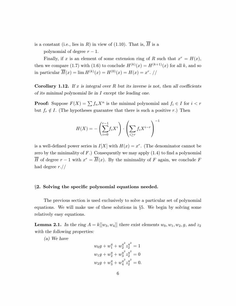
is a constant (i.e., lies in R) in view of (1.10). That is, H is a

polynomial of degree r − 1.

Finally, if x is an element of some extension ring of R such that xr = H(x),

then we compare (1.7) with (1.6) to conclude H(k)(x) = H(k+1)(x) for all k, and so

in particular H(x) = limH(k)(x) = H(0)(x) = H(x) = xr. //

Corollary 1.12. If x is integral over R but its inverse is not, then all coefficients

of its minimal polynomial lie in I except the leading one.

Proof: Suppose F (X) =∑fnX

n is the minimal polynomial and fi ∈ I for i < r

but fr /∈ I. (The hypotheses guarantee that there is such a positive r.) Then

H(X) = −(r−1∑i=0

fiXi

)·

∑i≥r

fiXi−r

−1

is a well-defined power series in I[X] with H(x) = xr. (The denominator cannot be

zero by the minimality of F .) Consequently we may apply (1.4) to find a polynomial

H of degree r − 1 with xr = H(x). By the minimality of F again, we conclude F

had degree r.//

§2. Solving the specific polynomial equations needed.

The previous section is used exclusively to solve a particular set of polynomial

equations. We will make use of these solutions in §5. We begin by solving some

relatively easy equations.

Lemma 2.1. In the ring A = k[[w3, w4]] there exist elements w0, w1, w2, g, and z2

with the following properties:

(a) We have

w0g +wq1 + wq2

2 zq2

2 = 1

w1g +wq2 + wq2

3 zq2

2 = 0

w2g +wq3 + wq2

4 zq2

2 = 0.

6

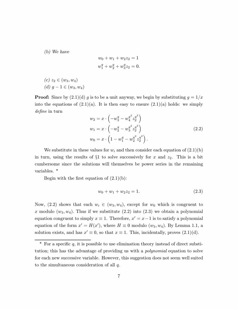
(b) We have

w0 +w1 + w2z2 = 1

wq1 +wq2 + wq3z2 = 0.

(c) z2 ∈ (w3, w4)

(d) g − 1 ∈ (w3, w4)

Proof: Since by (2.1)(d) g is to be a unit anyway, we begin by substituting g = 1/x

into the equations of (2.1)(a). It is then easy to ensure (2.1)(a) holds: we simply

define in turn

w2 = x ·(−wq3 − w

q2

4 zq2

2

)w1 = x ·

(−wq2 − w

q2

3 zq2

2

)w0 = x ·

(1−wq1 −w

q2

2 zq2

2

).

(2.2)

We substitute in these values for wi and then consider each equation of (2.1)(b)

in turn, using the results of §1 to solve successively for x and z2. This is a bit

cumbersome since the solutions will themselves be power series in the remaining

variables. *

Begin with the first equation of (2.1)(b):

w0 +w1 + w2z2 = 1. (2.3)

Now, (2.2) shows that each wi ∈ (w3, w4), except for w0 which is congruent to

x modulo (w3, w4). Thus if we substitute (2.2) into (2.3) we obtain a polynomial

equation congruent to simply x ≡ 1. Therefore, x′ = x−1 is to satisfy a polynomial

equation of the form x′ = H(x′), where H ≡ 0 modulo (w3, w4). By Lemma 1.1, a

solution exists, and has x′ ≡ 0, so that x ≡ 1. This, incidentally, proves (2.1)(d).

* For a specific q, it is possible to use elimination theory instead of direct substi-

tution; this has the advantage of providing us with a polynomial equation to solve

for each new successive variable. However, this suggestion does not seem well suited

to the simultaneous consideration of all q.

7

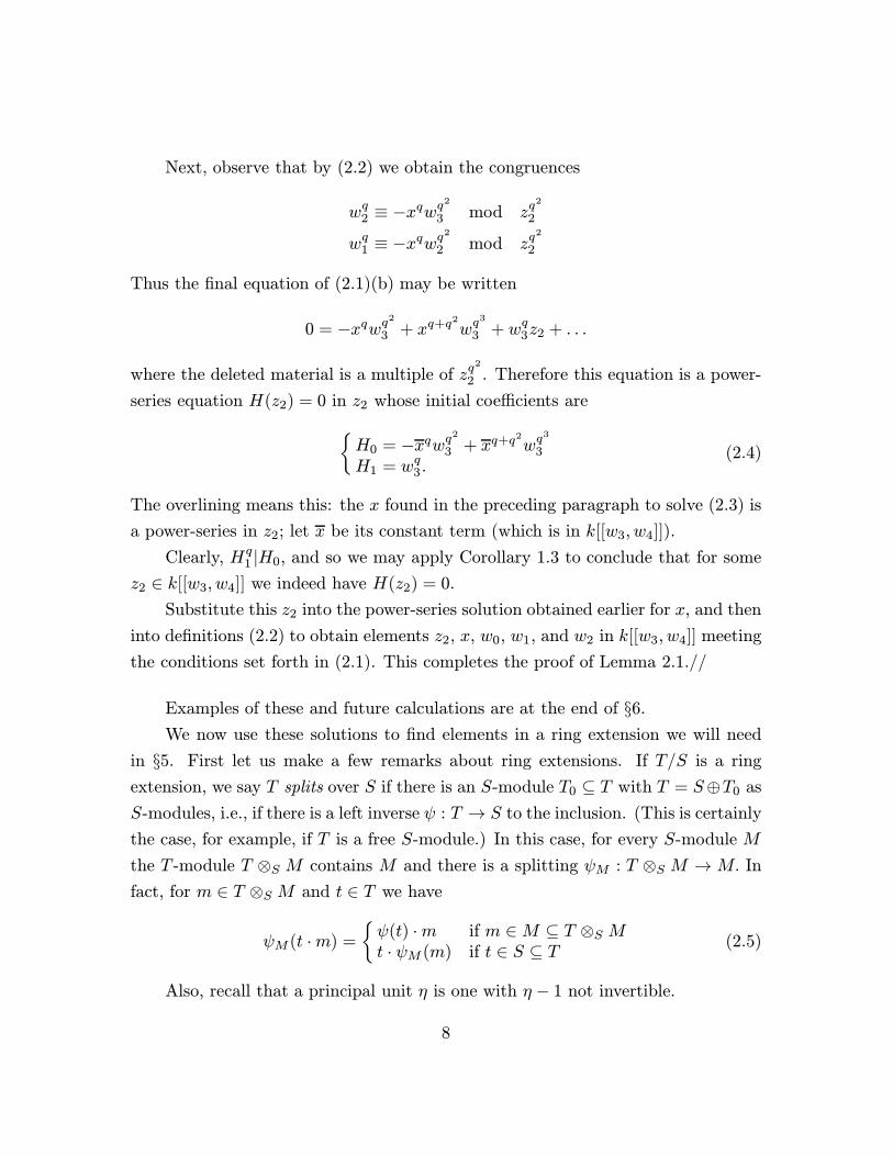
Next, observe that by (2.2) we obtain the congruences

wq2 ≡ −xqwq2

3 mod zq2

2

wq1 ≡ −xqwq2

2 mod zq2

2

Thus the final equation of (2.1)(b) may be written

0 = −xqwq2

3 + xq+q2

wq3

3 + wq3z2 + . . .

where the deleted material is a multiple of zq2

2 . Therefore this equation is a power-

series equation H(z2) = 0 in z2 whose initial coefficients are{H0 = −xqwq

2

3 + xq+q2

wq3

3

H1 = wq3.(2.4)

The overlining means this: the x found in the preceding paragraph to solve (2.3) is

a power-series in z2; let x be its constant term (which is in k[[w3, w4]]).

Clearly, Hq1 |H0, and so we may apply Corollary 1.3 to conclude that for some

z2 ∈ k[[w3, w4]] we indeed have H(z2) = 0.

Substitute this z2 into the power-series solution obtained earlier for x, and then

into definitions (2.2) to obtain elements z2, x, w0, w1, and w2 in k[[w3, w4]] meeting

the conditions set forth in (2.1). This completes the proof of Lemma 2.1.//

Examples of these and future calculations are at the end of §6.

We now use these solutions to find elements in a ring extension we will need

in §5. First let us make a few remarks about ring extensions. If T/S is a ring

extension, we say T splits over S if there is an S-module T0 ⊆ T with T = S⊕T0 as

S-modules, i.e., if there is a left inverse ψ : T → S to the inclusion. (This is certainly

the case, for example, if T is a free S-module.) In this case, for every S-module M

the T -module T ⊗S M contains M and there is a splitting ψM : T ⊗S M →M. In

fact, for m ∈ T ⊗S M and t ∈ T we have

ψM (t ·m) =

{ψ(t) ·m if m ∈M ⊆ T ⊗S Mt · ψM (m) if t ∈ S ⊆ T (2.5)

Also, recall that a principal unit η is one with η − 1 not invertible.

8

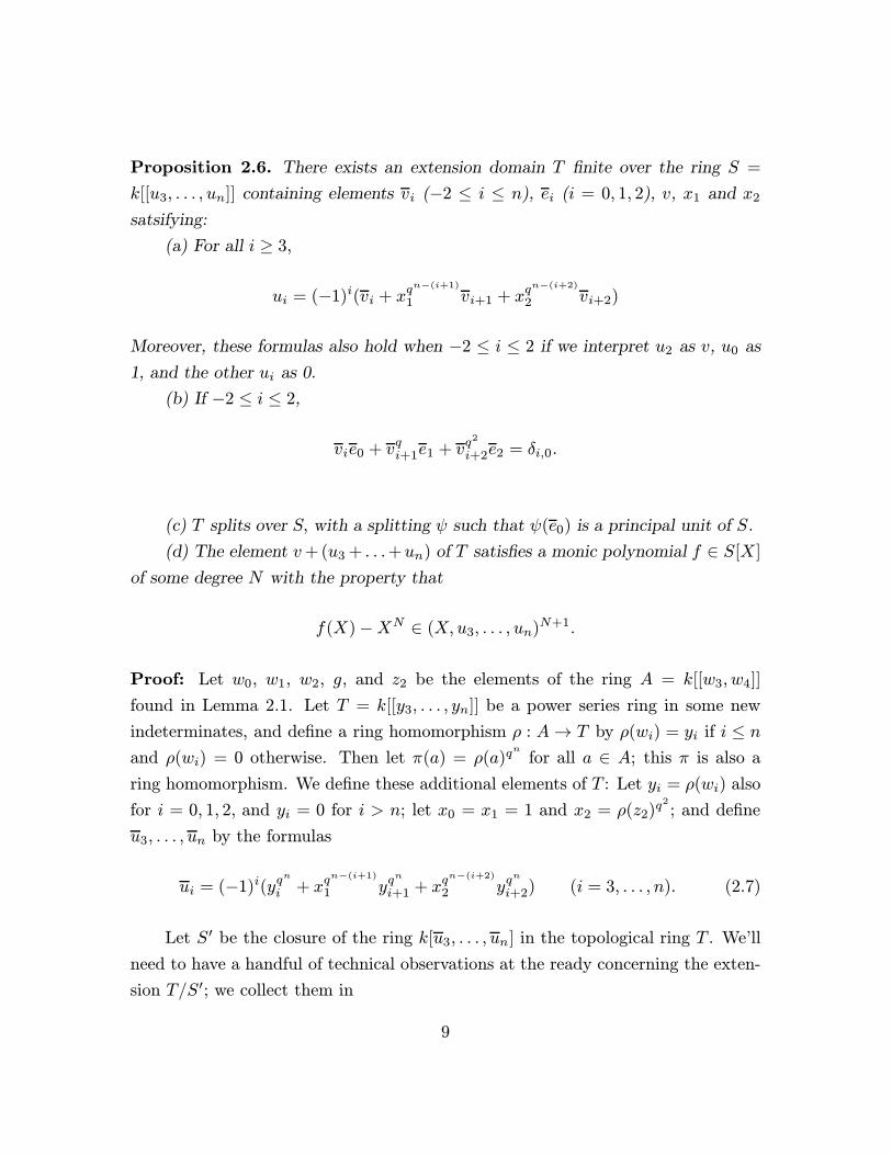
Proposition 2.6. There exists an extension domain T finite over the ring S =

k[[u3, . . . , un]] containing elements vi (−2 ≤ i ≤ n), ei (i = 0, 1, 2), v, x1 and x2

satsifying:

(a) For all i ≥ 3,

ui = (−1)i(vi + xqn−(i+1)

1 vi+1 + xqn−(i+2)

2 vi+2)

Moreover, these formulas also hold when −2 ≤ i ≤ 2 if we interpret u2 as v, u0 as

1, and the other ui as 0.

(b) If −2 ≤ i ≤ 2,

vie0 + vqi+1e1 + vq2

i+2e2 = δi,0.

(c) T splits over S, with a splitting ψ such that ψ(e0) is a principal unit of S.

(d) The element v+ (u3 + . . .+un) of T satisfies a monic polynomial f ∈ S[X]

of some degree N with the property that

f(X)−XN ∈ (X, u3, . . . , un)N+1.

Proof: Let w0, w1, w2, g, and z2 be the elements of the ring A = k[[w3, w4]]

found in Lemma 2.1. Let T = k[[y3, . . . , yn]] be a power series ring in some new

indeterminates, and define a ring homomorphism ρ : A→ T by ρ(wi) = yi if i ≤ nand ρ(wi) = 0 otherwise. Then let π(a) = ρ(a)q

n

for all a ∈ A; this π is also a

ring homomorphism. We define these additional elements of T : Let yi = ρ(wi) also

for i = 0, 1, 2, and yi = 0 for i > n; let x0 = x1 = 1 and x2 = ρ(z2)q2

; and define

u3, . . . , un by the formulas

ui = (−1)i(yqn

i + xqn−(i+1)

1 yqn

i+1 + xqn−(i+2)

2 yqn

i+2) (i = 3, . . . , n). (2.7)

Let S′ be the closure of the ring k[u3, . . . , un] in the topological ring T . We’ll

need to have a handful of technical observations at the ready concerning the exten-

sion T/S′; we collect them in

9

Lemma 2.8. S′ is isomorphic to the power-series ring S = k[[u3, . . . , un]]. T is an

integral domain, a finitely generated free S′-module, and an integral extension of

S′, in which the ideals (u3, . . . , un) and (yqn

3 , . . . , yqn

n ) coincide. There is a splitting

ψ : T → S′ carrying principal units of T to principal units of S′.

Proof: The obvious continuous homomorphism ui → ui from the polynomial ring

on a set of indeterminates ui to T extends to a surjection S → S′. To see that it is an

isomorphism, we need only ensure that the ui ∈ T are algebraically independent,

i.e., that S′ has the appropriate transcendence degree. This, in turn, will follow

from showing that T is a finite S′-module.

Clearly, T = k[[y3, . . . , yn]] is an integral domain, so that un ∈ T is not a

zero-divisor on T . I claim more strongly that un, . . . , u3 is a regular sequence on T .

Indeed, from equation (2.7), it follows by induction that T/(un, . . . , ui) is isomorphic

to the quotient k[[y3, . . . , yn]]/(yqn

n , . . . , yqn

i ); the image of ui−1 here is ±yqn

i−1, which

is clearly not a zero-divisor. Proceeding down to i = 3, we conclude that T

is a free S′-module. Indeed, a set of module generators is evidently the set of

products yI =∏ymii with each mi < qn. Thus T/S′ is finite, and in particular

integral.

Similarly, equation (2.7) shows each (ui, . . . , un) = (yqn

i , . . . , yqn

n ) by downward

induction on i.

An obvious splitting ψ : T → S′ takes an element ε =∑aIy

I to aO. Clearly

aO ≡ ε modulo (y1, . . . , yn); in particular if ε is a principal unit in T , then 1 ≡ ε ≡aO, so aO is itself a principal unit in S.//

We will identify the rings S and S′, so that we may view T as an extension of

S, in which the elements ui satisfy (2.7).

Now that we have an extension T of the ring S, we need to find elements in

it with the desired properties. Use (2.6)(a) as the definition of the vi for i ≥ −2.

Define e0 = π(g) and ek = xqn

k for k > 0, and define v by

v = yqn

2 + xqn−3

1 yqn

3 + xqn−4

2 yqn

4 (2.9)

Comparing (2.7) and (2.9) to the definition (2.6)(a) of the vi shows that vi = yqn

i

for i ≥ 2.

10

If we apply π to the equations of Lemma 2.1, we get relations among these

elements of T :

yqn

0 e0 + yqn+1

1 e1 + yqn+2

2 e2 = 1

yqn

1 e0 + yqn+1

2 e1 + yqn+2

3 e2 = 0

yqn

2 e0 + yqn+1

3 e1 + yqn+2

4 e2 = 0

(2.10)

yqn

0 + xqn−1

1 yqn

1 + xqn−2

2 yqn

2 = 1

yqn+1

1 + xqn−1

1 yqn+1

2 + xqn−2

2 yqn+1

3 = 0(2.11)

Comparing (2.11) to (2.6)(a) shows now that vi = yqn

i also for i ≥ 0. Then (2.10)

shows that (2.6)(b) holds for all i = 0, 1, 2.

However, I will show by induction that (2.6)(b) also holds for negative i. Indeed,

if for i0 = −1 or −2 we know (2.6)(b) to be true whenever i > i0, then for i = i0

we calculate

(vie0 + vqi+1e1 + vq

2

i+2e2

)=

j=2∑j=0

(vi+je0 + vqi+j+1e1 + vq

2

i+j+2e2

)xq

n−i−j

j − xqn

−i

=k=2∑k=0

ek

j=2∑j=0

vi+k+jxqn−(i+k+j)

j

qk

− xqn

−i

=k=2∑k=0

(ek)(δi+k,0)− xqn

−i = 0.

(The penultimate inequality comes from the definition (2.6)(a) of vi+k.) So indeed

(2.6)(b) holds for i < 0.

Next we prove Prop. 2.6(d). We first estimate v as follows. From (2.1)(c)

it follows x2 lies in the ideal I ′ = (y3, . . . , yn) (while x0 = x1 = 1). Of course,

each yqn

i lies in I = (yqn

3 , . . . , yqn

n ) = (u3, . . . un) so if we add all the equations

of (2.7) to (2.9) and reduce modulo II ′, we have only a telescoping sum giving

r := v + (u3 + . . . + un) ≡ yqn

2 = π(w2). Since g is a unit by (2.1)(d), the last

equation of (2.1)(a) shows w2 lies in (w3, w4)q, so that certainly π(w2) ≡ 0, and

hence r ∈ II ′.Now since T/S is finite, let f ∈ S[X] be a monic polynomial of minimal

11

degree N satisfied by r. Certainly the constant term is not invertible in S, as it

is a multiple of r ∈ II ′. But then it follows from Corollary 1.12 that no coefficient

other than that of XN is invertible. Then the ring of integers S in a splitting field

of f is again a local ring with maximal ideal I, say. Certainly I is preserved under

automorphisms of S, as is I = (u3, . . . , un); so since r ∈ II and each conjugate

of r also lies in II. Then f is the product of conjugates of (X − r), and hence

the coefficient of XN−i lies in (II)i ∩ S ⊆ IiI ∩ S = (I ∩ S)i+1, as required for

Prop. 2.6(d).

Finally, by (2.1)(d), g is a principal unit in A, so that e0 = π(g) is a principal

unit in T . By Lemma 2.8, ψ(e0) is also a principal unit. This completes the proof

of the proposition. //

§3. The Steenrod algebra A.

We will need in §§5–6 to have some nicely-behaved endomorphisms of M which

can play the role of those mentioned in the introduction operating on

k[X1, . . . , Xn]. In view of the intended applications, we draw them in part from

the Steenrod algebra.

We first need to construct an analogue (of a suitable subalgebra) over all finite

fields k. Suppose k has q = pr elements, with p an odd prime. (The assertions

of this section also hold when p = 2 if the customary modifications are made.)

Let B be the subalgebra of the ordinary mod-p Steenrod algebra generated by the

reduced-power operations Pi, and let B∗ = Hom(B,Fp) be its dual. Then B∗ has a

natural product structure under which it is a polynomial ring Fp[ξ1, ξ2, . . .] (see [M]

for details). It then has a basis consisting of the monomials ξI = ξi11 ξi22 . . .; write

αI for the corresponding element of the dual basis of B.

Definition 3.1. (a) Let I ⊆ B∗ ⊗ k = (B⊗ k)∗ be the ideal generated by all ξt⊗ 1

with r 6 | t.(b) Define the Steenrod algebra over k to be the subspace A ⊆ B⊗k orthogonal

to I.

(c) Let ψt = ξrt ⊗ 1 ∈ (B ⊗ k)∗. (But see Notation 3.4)

12

Thus, when k = Fp, A coincides with B. We now want to establish that the

following properties hold for all fields k; that they hold when k = Fp is shown in

[M]. We write ψI for a product ψi11 ψi22 . . .; clearly these products form a basis for

(B ⊗ k)∗/I, so that the duals ψI ∈ B ⊗ k form a basis of A.

Proposition 3.2. (a) A acts naturally on cohomology rings H∗(X, k) over k; the

Cartan formula

ψI(x · y) =∑

I=J+K

ψJ(x) · ψK(y) (3.3)

holds for all x and y in H∗(X, k).

(b) A acts on every polynomial ring k[X1, . . . , Xn] in such a way that for every

v linear in the Xi, we have

ψI(v) =

{vqt

if ψI = ψt0 otherwise

Moreover, the action of A commutes with that of GL(n, k).

Proof: (a) The action A on H∗(X, k) = H∗(X,Fp) ⊗ k is inherited from the

inclusion A ⊆ B⊗k. The action on products derives ¿from the coproduct on B⊗k,

and so from the coproduct on B, which is

∆(αI) =∑

αJ ⊗ αK ;

it is clear from Definition 3.1(b) that the span A of the ψI is then a sub-comodule

of B ⊗ k.

(b) The action follows from (a) above, since k[X1, . . . , Xn] ' H∗(BTn, k). If

{ej : 1 ≤ j ≤ r} is a basis of k over Fp, then the “linear” terms v are Fp-linear

combinations of the Xi ⊗ ej ∈ H∗(BTn,Fp)⊗ k. Since, from [M] we have

(αI ⊗ 1)(Xi ⊗ ej) =

{Xpt

i ⊗ ej if ξI = ξt0 otherwise,

we indeed have ψI(Xi ⊗ ej) = 0 except (since eq = e for every e ∈ k!)

ψt(Xi ⊗ ej) = (ξrt ⊗ 1)(Xi ⊗ ej) = Xprt

i ⊗ ej = (Xi ⊗ ej)qt

13

as desired.

If g ∈ GL(n, k), we have (g(v))qt

= g(vqt

), so the actions of A and GL(n, k)

commute on all linear classes. We then use the Cartan formula and linearity to see

that they commute everywhere. //

It follows from (3.2)(d) that A acts on the Dickson algebra D.

We will say that a D-module M admits an A-module structure (respecting

that of D) if the Cartan formula (3.3) holds for all x ∈ D and y ∈ M . This is the

setting in which the main theorem holds. (By Prop. 3.2(a) and (b), this is certainly

the case if M = H∗(X,Fp) and D is a subring of M , or if M = k[X1, . . . , Xn]G for

a subgroup G ⊆ GL(n, k), since then again D ⊆M ; therefore the Main Theorem is

applicable to the situations described in the introduction.)

Notation 3.4. To agree with the classical case, we will henceforth write ξI and αI

in lieu of ψI and ψI for the basis elements of A∗ and A respectively.

In the proof of the main theorem, we will need to have homomorphisms of D

and the D-module M of a very special type. We would like to form them using only

the homomorphisms of the Steenrod algebra and multiplication by elements of the

ring D. However, in order to make use of the “multiplicative” maps below, we need

to allow ourselves to make reference to some extension rings of D.

Definition 3.5. (a) Let D =∏m≥0D

m, where Dm is the set of polynomials in

D ⊆ k[X1, . . . , Xn] of degree m in the Xi. Similarly,

(b) Let M =∏m≥0M

m.

(c) If R is any commutative extension of D, let MR = R⊗D M .

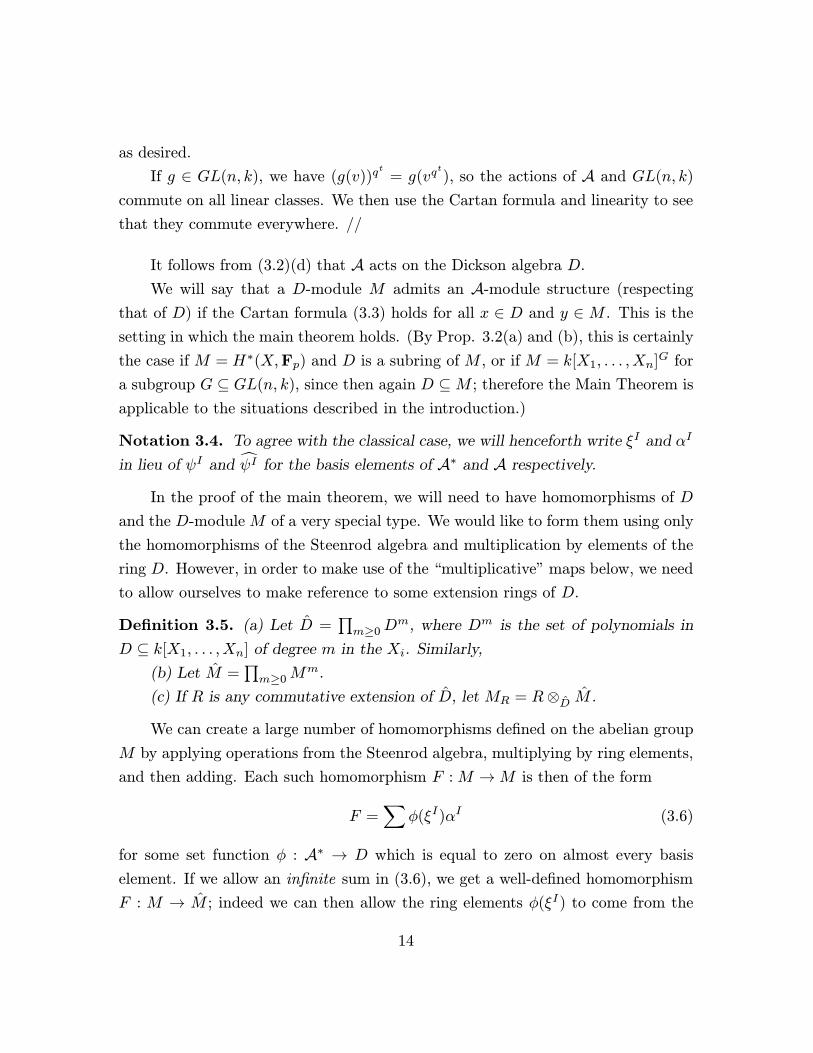
We can create a large number of homomorphisms defined on the abelian group

M by applying operations from the Steenrod algebra, multiplying by ring elements,

and then adding. Each such homomorphism F : M →M is then of the form

F =∑

φ(ξI)αI (3.6)

for some set function φ : A∗ → D which is equal to zero on almost every basis

element. If we allow an infinite sum in (3.6), we get a well-defined homomorphism

F : M → M ; indeed we can then allow the ring elements φ(ξI) to come from the

14

larger ring D, since A is a locally-finite graded algebra. If next we allow these

ring elements to be chosen from the yet-larger ring R, F becomes a well-defined

homomorphism F : M → MR. We do not need to assume that A acts on R since

we will only apply F to elements in M , not in MR.

Observe that if M is the D-module D, then M = D and MR = R. Note that

any F defined by formula (3.6) also defines homomorphisms defined on D. Now,

while the formula (3.6) gives well-defined maps when φ is any set function, we can

say more when φ preserves multiplication:

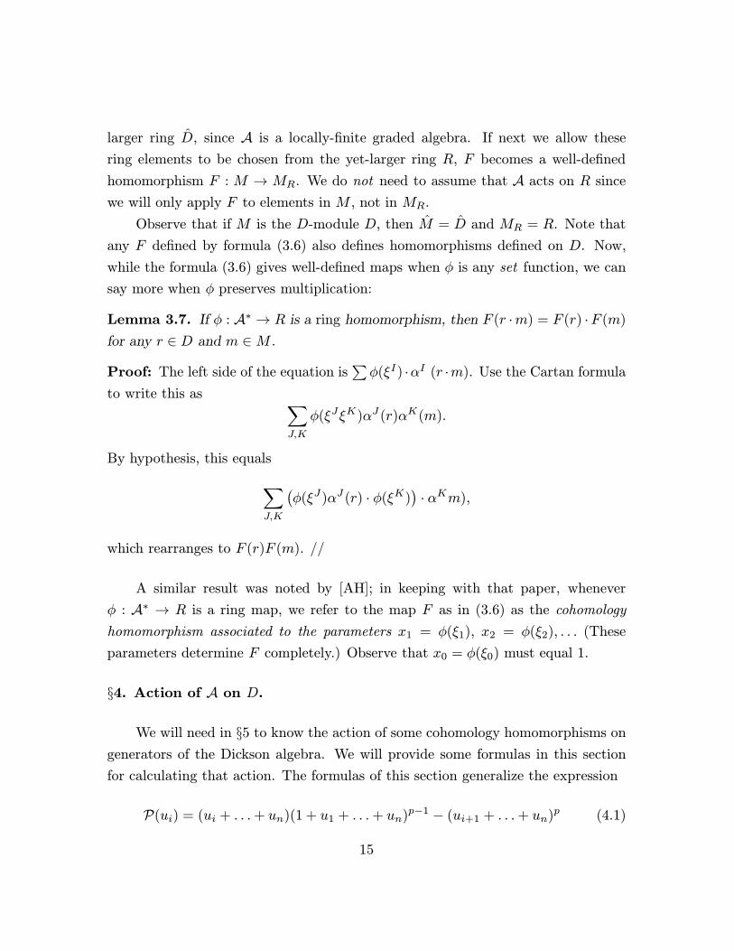
Lemma 3.7. If φ : A∗ → R is a ring homomorphism, then F (r ·m) = F (r) ·F (m)

for any r ∈ D and m ∈M .

Proof: The left side of the equation is∑φ(ξI) ·αI (r ·m). Use the Cartan formula

to write this as ∑J,K

φ(ξJξK)αJ (r)αK(m).

By hypothesis, this equals∑J,K

(φ(ξJ)αJ (r) · φ(ξK)

)· αKm),

which rearranges to F (r)F (m). //

A similar result was noted by [AH]; in keeping with that paper, whenever

φ : A∗ → R is a ring map, we refer to the map F as in (3.6) as the cohomology

homomorphism associated to the parameters x1 = φ(ξ1), x2 = φ(ξ2), . . . (These

parameters determine F completely.) Observe that x0 = φ(ξ0) must equal 1.

§4. Action of A on D.

We will need in §5 to know the action of some cohomology homomorphisms on

generators of the Dickson algebra. We will provide some formulas in this section

for calculating that action. The formulas of this section generalize the expression

P(ui) = (ui + . . .+ un)(1 + u1 + . . .+ un)p−1 − (ui+1 + . . .+ un)p (4.1)

15

of Landweber and Stong [LSD]. The basis of the argument is fairly standard (see

e.g. Wilkerson [W]).

We first recall that the Dickson invariants ui ∈ D may be defined using the

expansion of a certain polynomial E ∈ D[X] :

E(X) =∏v∈V

(X − v) =∑

0≤i≤n(−1)iuiX

qn−i (4.2)

where V is the Fq-linear span of X1, . . . , Xn. (This includes the definition u0 = 1.)

We also make the following easy observation.

Lemma 4.3. Suppose R is a ring containing Fq, and that the polynomial P ∈ R[Z]

is fixed. Then the following are equivalent:

(a) P (Z) =∑aiZ

qi for some set of ai ∈ R.(b) P : R→ R is Fq-linear.

(c) The roots of P form an Fq vector-space.

Proof: That (a) implies (b) is obvious, and that (b) implies (c) follows from

applying P to sums and scalar multiples of roots of P . To see that (c) implies (a),

let V be the vector space of roots, and let S(V ) ≡ k[X1, . . . , Xn] be the symmetric

algebra on V. Then any splitting field k of P containing R will also contain a

homomorphic image of S(V ). Then P ∈ k[Z] is the image of a scalar multiple of

H(Z) =∏v∈V (Z − v) ∈ S(V )[Z]. But equation (4.2) shows that all coefficients of

H (and thus of P ) vanish except those of Zqi

. //

Now we can determine the action of A on D:

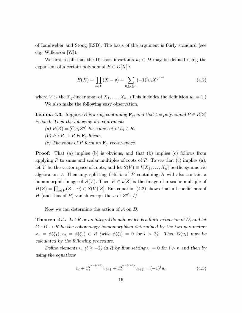
Theorem 4.4. Let R be an integral domain which is a finite extension of D, and let

G : D → R be the cohomology homomorphism determined by the two parameters

x1 = φ(ξ1), x2 = φ(ξ2) ∈ R (with φ(ξi) = 0 for i > 2). Then G(ui) may be

calculated by the following procedure.

Define elements vi (i ≥ −2) in R by first setting vi = 0 for i > n and then by

using the equations

vi + xqn−(i+1)

1 vi+1 + xqn−(i+2)

2 vi+2 = (−1)iui (4.5)

16

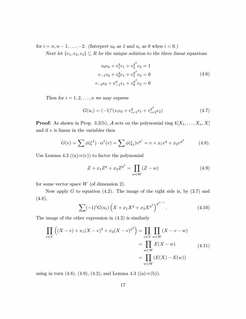
for i = n, n− 1, . . . ,−2. (Interpret u0 as 1 and ui as 0 when i < 0.)

Next let {e1, e2, e3} ⊆ R be the unique solution to the three linear equations

v0e0 + vq1e1 + vq2

2 e2 = 1

v−1e0 + vq0e1 + vq2

1 e2 = 0

v−2e0 + vq−1e1 + vq2

0 e2 = 0

(4.6)

Then for i = 1, 2, . . . , n we may express

G(ui) = (−1)i(vie0 + vqi+1e1 + vq2

i+2e2) (4.7)

Proof: As shown in Prop. 3.2(b), A acts on the polynomial ring k[X1, . . . , Xn, X]

and if v is linear in the variables then

G(v) =∑

φ(ξI) · αI(v) =∑

φ(ξj)vqj = v + x1v

q + x2vq2

(4.8).

Use Lemma 4.3 ((a)⇒(c)) to factor the polynomial

Z + x1Zq + x2Z

q2

=∏w∈W

(Z − w) (4.9)

for some vector space W (of dimension 2).

Now apply G to equation (4.2). The image of the right side is, by (3.7) and

(4.8), ∑(−1)iG(ui)

(X + x1X

q + x2Xq2)qn−i

. (4.10)

The image of the other expression in (4.2) is similarly∏v∈V

((X − v) + x1(X − v)2 + x2(X − v)q

2)

=∏v∈V

∏w∈W

(X − v −w)

=∏w∈W

E(X − w)

=∏w∈W

(E(X)−E(w))

(4.11)

using in turn (4.8), (4.9), (4.2), and Lemma 4.3 ((a)⇒(b)).

17

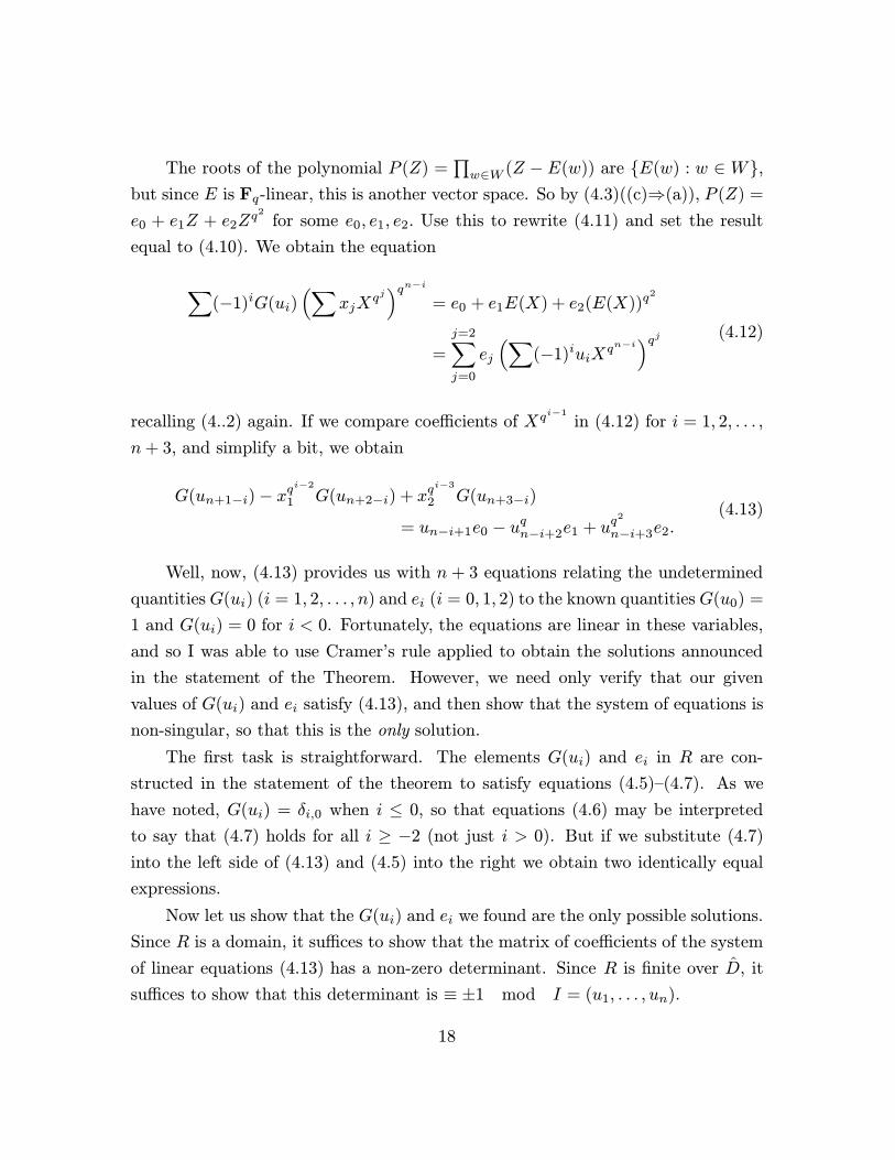
The roots of the polynomial P (Z) =∏w∈W (Z − E(w)) are {E(w) : w ∈ W},

but since E is Fq-linear, this is another vector space. So by (4.3)((c)⇒(a)), P (Z) =

e0 + e1Z + e2Zq2

for some e0, e1, e2. Use this to rewrite (4.11) and set the result

equal to (4.10). We obtain the equation

∑(−1)iG(ui)

(∑xjX

qj)qn−i

= e0 + e1E(X) + e2(E(X))q2

=

j=2∑j=0

ej

(∑(−1)iuiX

qn−i)qj (4.12)

recalling (4..2) again. If we compare coefficients of Xqi−1

in (4.12) for i = 1, 2, . . . ,

n+ 3, and simplify a bit, we obtain

G(un+1−i)− xqi−2

1 G(un+2−i) + xqi−3

2 G(un+3−i)

= un−i+1e0 − uqn−i+2e1 + uq2

n−i+3e2.(4.13)

Well, now, (4.13) provides us with n + 3 equations relating the undetermined

quantitiesG(ui) (i = 1, 2, . . . , n) and ei (i = 0, 1, 2) to the known quantitiesG(u0) =

1 and G(ui) = 0 for i < 0. Fortunately, the equations are linear in these variables,

and so I was able to use Cramer’s rule applied to obtain the solutions announced

in the statement of the Theorem. However, we need only verify that our given

values of G(ui) and ei satisfy (4.13), and then show that the system of equations is

non-singular, so that this is the only solution.

The first task is straightforward. The elements G(ui) and ei in R are con-

structed in the statement of the theorem to satisfy equations (4.5)–(4.7). As we

have noted, G(ui) = δi,0 when i ≤ 0, so that equations (4.6) may be interpreted

to say that (4.7) holds for all i ≥ −2 (not just i > 0). But if we substitute (4.7)

into the left side of (4.13) and (4.5) into the right we obtain two identically equal

expressions.

Now let us show that the G(ui) and ei we found are the only possible solutions.

Since R is a domain, it suffices to show that the matrix of coefficients of the system

of linear equations (4.13) has a non-zero determinant. Since R is finite over D, it

suffices to show that this determinant is ≡ ±1 mod I = (u1, . . . , un).

18

But indeed, this matrix of coefficients is nearly lower-triangular. When reduced

modulo I, the ith equation only involves the (i− 2)nd , (i− 1)st , and ith variables.

(Here I am ordering them as: G(un), G(un−1), . . . , G(u1); e0, e1, e2.) The determi-

nant is then the product of the diagonal entries, each of which is 1 or a power of

±u0 = ±1, so that the product is indeed ±1. claims.) //

An argument similar to the one concluding this proof establishes that there

really is a unique solution {ei} to the equations (4.6), as claimed in the statement

of the theorem.

The reader may wish to verify that (4.1) is indeed a special case of Theo-

rem 4.4. It is the case with x0 = x1 = 1 and x2 = 0 ∈ D. Here we have

vi = (−1)i(ui + . . .+ un), e0 = (1 + u1 + . . .+ un)q−1, e1 = 1, and e2 = 0.

§5. Existence of a suitable endomorphism of M .

In the proof of the Main Theorem, we will need to have an endomorphism of

the module with a few very special properties. In essence, we need it to make the

images of the Dickson classes u1 and u2 nearly vanish. We will use the solutions

from §2 to define our homomorphisms, and then observe from the formulas in §4that the vanishing is guaranteed.

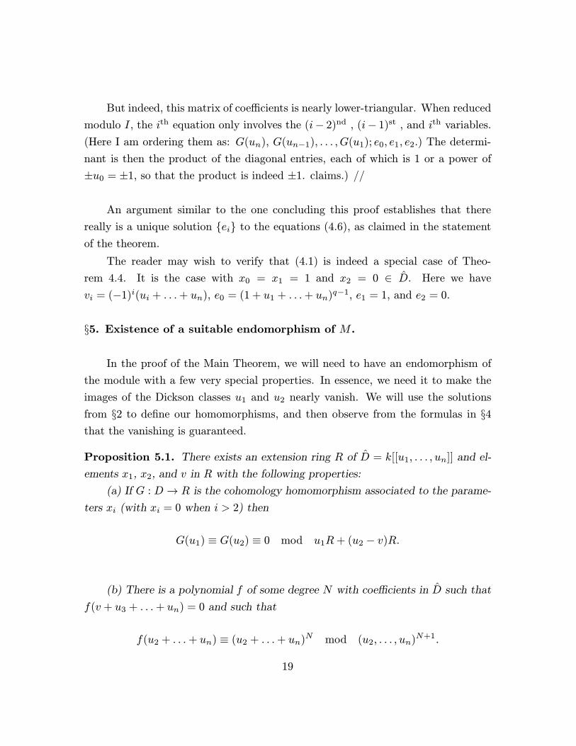
Proposition 5.1. There exists an extension ring R of D = k[[u1, . . . , un]] and el-

ements x1, x2, and v in R with the following properties:

(a) If G : D → R is the cohomology homomorphism associated to the parame-

ters xi (with xi = 0 when i > 2) then

G(u1) ≡ G(u2) ≡ 0 mod u1R+ (u2 − v)R.

(b) There is a polynomial f of some degree N with coefficients in D such that

f(v + u3 + . . .+ un) = 0 and such that

f(u2 + . . .+ un) ≡ (u2 + . . .+ un)N mod (u2, . . . , un)N+1.

19

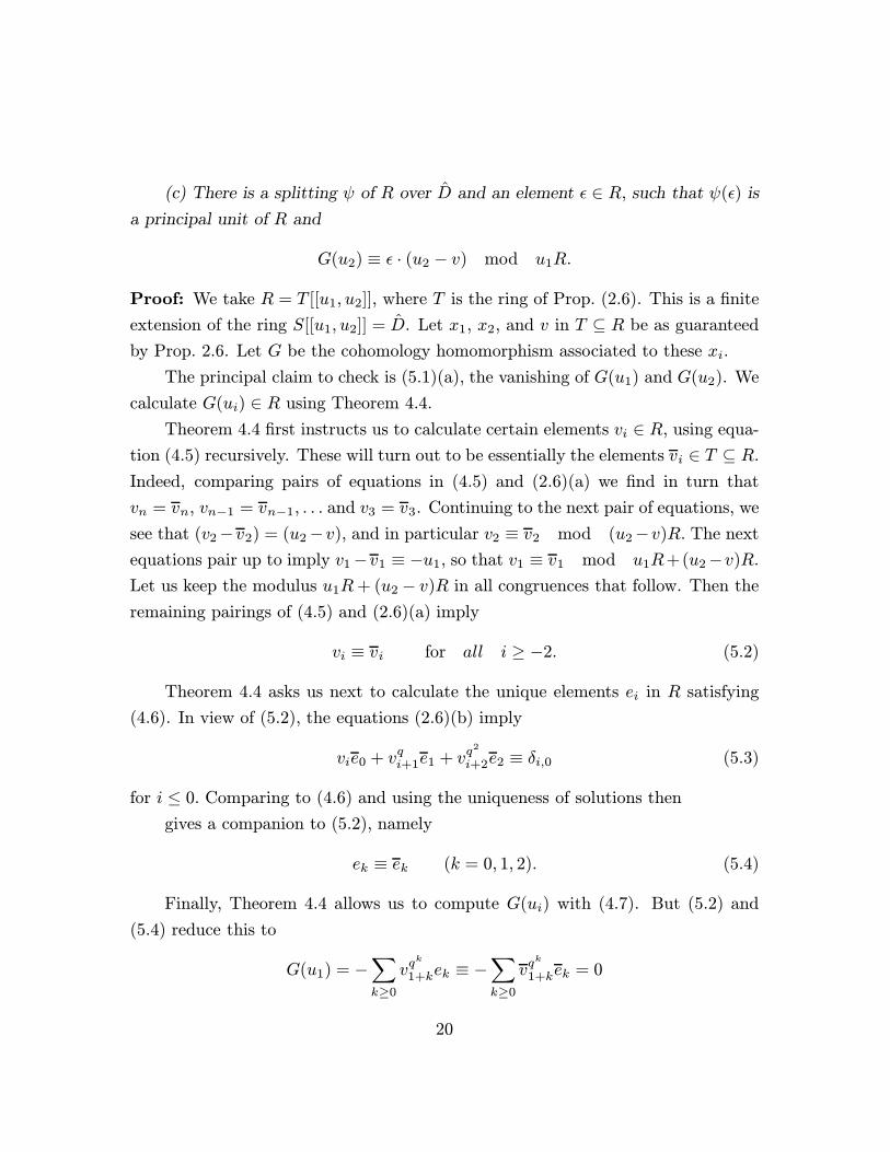
(c) There is a splitting ψ of R over D and an element ε ∈ R, such that ψ(ε) is

a principal unit of R and

G(u2) ≡ ε · (u2 − v) mod u1R.

Proof: We take R = T [[u1, u2]], where T is the ring of Prop. (2.6). This is a finite

extension of the ring S[[u1, u2]] = D. Let x1, x2, and v in T ⊆ R be as guaranteed

by Prop. 2.6. Let G be the cohomology homomorphism associated to these xi.

The principal claim to check is (5.1)(a), the vanishing of G(u1) and G(u2). We

calculate G(ui) ∈ R using Theorem 4.4.

Theorem 4.4 first instructs us to calculate certain elements vi ∈ R, using equa-

tion (4.5) recursively. These will turn out to be essentially the elements vi ∈ T ⊆ R.

Indeed, comparing pairs of equations in (4.5) and (2.6)(a) we find in turn that

vn = vn, vn−1 = vn−1, . . . and v3 = v3. Continuing to the next pair of equations, we

see that (v2−v2) = (u2−v), and in particular v2 ≡ v2 mod (u2−v)R. The next

equations pair up to imply v1−v1 ≡ −u1, so that v1 ≡ v1 mod u1R+(u2−v)R.

Let us keep the modulus u1R+ (u2 − v)R in all congruences that follow. Then the

remaining pairings of (4.5) and (2.6)(a) imply

vi ≡ vi for all i ≥ −2. (5.2)

Theorem 4.4 asks us next to calculate the unique elements ei in R satisfying

(4.6). In view of (5.2), the equations (2.6)(b) imply

vie0 + vqi+1e1 + vq2

i+2e2 ≡ δi,0 (5.3)

for i ≤ 0. Comparing to (4.6) and using the uniqueness of solutions then

gives a companion to (5.2), namely

ek ≡ ek (k = 0, 1, 2). (5.4)

Finally, Theorem 4.4 allows us to compute G(ui) with (4.7). But (5.2) and

(5.4) reduce this to

G(u1) = −∑k≥0

vqk

1+kek ≡ −∑k≥0

vqk

1+kek = 0

20

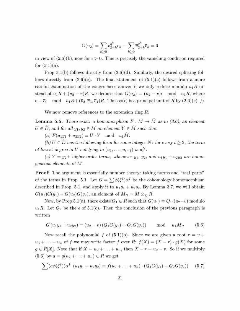
G(u2) =∑k≥0

vqk

2+kek ≡∑k≥0

vqk

2+kek = 0

in view of (2.6)(b), now for i > 0. This is precisely the vanishing condition required

for (5.1)(a).

Prop 5.1(b) follows directly from (2.6)(d). Similarly, the desired splitting fol-

lows directly from (2.6)(c). The final statement of (5.1)(c) follows from a more

careful examination of the congruences above: if we only reduce modulo u1R in-

stead of u1R + (u2 − v)R, we deduce that G(u2) ≡ (u2 − v)ε mod u1R, where

ε ≡ e0 mod u1R+(v2, v3, v4)R. Thus ψ(ε) is a principal unit of R by (2.6)(c). //

We now remove references to the extension ring R.

Lemma 5.5. There exist: a homomorphism F : M → M as in (3.6), an element

U ∈ D, and for all y1, y2 ∈M an element Y ∈ M such that

(a) F (u1y1 + u2y2) ≡ U · Y mod u1M.

(b) U ∈ D has the following form for some integer N : for every t ≥ 2, the term

of lowest degree in U not lying in (u1, . . . , ut−1) is uNt .

(c) Y = y2+ higher-order terms, whenever y1, y2, and u1y1 + u2y2 are homo-

geneous elements of M .

Proof: The argument is essentially number theory: taking norms and “real parts”

of the terms in Prop. 5.1. Let G =∑φ(ξI)αI be the cohomology homomorphism

described in Prop. 5.1, and apply it to u1y1 + u2y2. By Lemma 3.7, we will obtain

G(u1)G(y1) +G(u2)G(y2), an element of MR = M ⊗D R.

Now, by Prop 5.1(a), there existsQ1 ∈ R such thatG(u1) ≡ Q1·(u2−v) modulo

u1R. Let Q2 be the ε of 5.1(c). Then the conclusion of the previous paragraph is

written

G (u1y1 + u2y2) ≡ (u2 − v) (Q1G(y1) +Q2G(y2)) mod u1MR (5.6)

Now recall the polynomial f of (5.1)(b). Since we are given a root r = v +

u3 + . . .+ un of f we may write factor f over R: f(X) = (X − r) · g(X) for some

g ∈ R[X]. Note that if X = u2 + . . .+ un, then X − r = u2 − v. So if we multiply

(5.6) by a = g(u2 + . . .+ un) ∈ R we get∑(aφ(ξI))αI (u1y1 + u2y2) ≡ f(u2 + . . .+ un) · (Q1G(y1) +Q2G(y2)) (5.7)

21

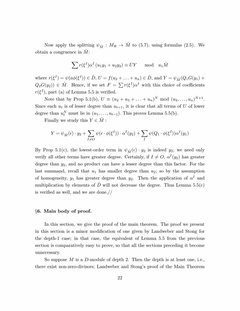
Now apply the splitting ψM : MR → M to (5.7), using formulas (2.5). We

obtain a congruence in M :∑r(ξI)αI (u1y1 + u2y2) ≡ UY mod u1M

where r(ξI) = ψ(aφ(ξI)) ∈ D, U = f(u2 + . . .+ un) ∈ D, and Y = ψM (Q1G(y1) +

Q2G(y2)) ∈ M . Hence, if we set F =∑r(ξI)αI with this choice of coefficients

r(ξI), part (a) of Lemma 5.5 is verified.

Note that by Prop 5.1(b), U ≡ (u2 + u3 + . . . + un)N mod (u2, . . . , un)N+1.

Since each ut is of lesser degree than ut+1, it is clear that all terms of U of lower

degree than uNt must lie in (u1, . . . , ut−1). This proves Lemma 5.5(b).

Finally we study this Y ∈ M :

Y = ψM (ε) · y2 +∑I 6=O

ψ(ε · φ(ξI)) · αI(y2) +∑I

ψ(Q1 · φ(ξI))αI(y1)

By Prop 5.1(c), the lowest-order term in ψM (ε) · y2 is indeed y2; we need only

verify all other terms have greater degree. Certainly, if I 6= O, αI(y2) has greater

degree than y2, and no product can have a lesser degree than this factor. For the

last summand, recall that u1 has smaller degree than u2; so by the assumption

of homogeneity, y1 has greater degree than y2. Then the application of αI and

multiplication by elements of D will not decrease the degree. Thus Lemma 5.5(c)

is verified as well, and we are done.//

§6. Main body of proof.

In this section, we give the proof of the main theorem. The proof we present

in this section is a minor modification of one given by Landweber and Stong for

the depth-1 case; in that case, the equivalent of Lemma 5.5 from the previous

section is comparatively easy to prove, so that all the sections preceding it become

unnecessary.

So suppose M is a D-module of depth 2. Then the depth is at least one, i.e.,

there exist non-zero-divisors; Landweber and Stong’s proof of the Main Theorem

22

in this case ensures u1 is not a zero-divisor. Since all maximal regular sequences

have the same length [Ma], we know there exists a non-zero-divisor on M/(u1M).

We want to show u2 is in fact not a zero-divisor there to prove the main theorem.

Thus the Main Theorem may be recast in this case as

Theorem 6.1. If M is a D-module with A-module structure, and u2 is a zero-

divisor on M/(u1M), then every element of (u1, . . . , un) is a zero-divisor as well.

Proof: We are assuming the presence of a homogeneous equation

0 = u1y1 + u2y2 (6.2)

with y1, y2 ∈M but y2 not in the submodule u1M .

We wish to obtain from (6.2) other equations that show other elements of I

are also zero-divisors on M/u1M . To do so we will apply the homomorphism F of

Lemma 5.5 to both sides of (6.2) and obtain a congruence

0 ≡ UY mod u1M. (6.3)

Let Jt = (u1, . . . , ut−1).

Lemma 6.4. For each t there is an integer k with Jkt · Y ≡ 0 modulo u1M .

Proof: The cases t ≤ 2 are trivial, as J1 = (0) and J2 = (u1); so we may proceed

by induction and assume Lemma 6.4 holds for some value t. Let us prove it holds

for t+ 1.

Multiply (6.3) by a power of U to obtain a congruence

0 ≡ UqrY mod u1M. (6.5)

We may assume qr > k, so that every summand of U ∈ D will only occur in (6.5)

raised to at least the kth power. Then by the inductive hypothesis, the summands

which lie in Jt annihilate Y (modulo u1M). Striking these terms from (6.5) leaves

a congruence

0 ≡ V qrY mod u1M (6.6)

in which (by Lemma 5.5(b)) the lowest-order term of V is uNt . Since the next

non-zero term of V qr

is then of substantially higher degree than uNqr

t , it follows

23

that the congruence (6.6) agrees with the congruence 0 ≡ uNqr

t · Y to many terms.

Certainly, then, the first qr terms of Y ∈ M are annihilated (modulo u1M) by this

large power of ut.

Taking increasingly large values of r in this argument, we conclude that every

homogeneous component of Y lies in⋃l≥0

{m ∈M : ultm ∈ u1M

}.

Since M is Noetherian, this increasing union of submodules must terminate, and so

for some single l, we must have ult · Y ≡ 0 (modulo u1M).

Combining this and the inductive hypothesis shows Jmt+1 · Y ≡ 0

modulo u1M for some m. This completes the inductive step. //

We may then in particular apply Lemma 6.4 when t = n + 1. Using also

Lemma 5.5(c), we then see that, for some k,

Jkn+1 · y2 ≡ 0 mod u1M.

Therefore, given any u ∈ Jn+1 = (u1, . . . , un), the sequence

y2, uy2, . . . , uky2

begins with a non-zero element of M/(u1M) but ends in zero. Thus, each such u is

a zero-divisor on M/(u1M), as was to be shown. //

This completes the proof of Theorem 6.1, and so of the Main Theorem.

The proof of the depth conjecture for s = 1 is essentially identical. For the

map F of Lemma 5.5, we may in this case take the total reduced power operation

P. The Cartan formula implies P(u1y1) = P(u1)P(y1) = UY, so the equivalent of

claim (a) is satisfied. Part (b) follows from the action of the Steenrod algebra on D

given in (4.1), so that (b) holds with N = 1. Part (c) is trivial, as P(y1) = y1 + . . ..

To give an example for the case (s = 2) at hand, suppose q = 2 and n = 4.

The solutions to the equations (2.1) found using the method of §1 are,

24

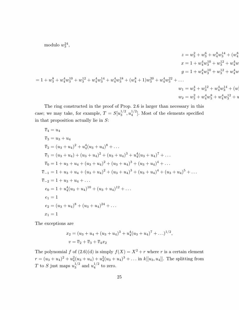
modulo w243 ,

z = w23 + w6

3 +w84w

143 + (w8

4

x = 1 + w44w

103 + w12

3 + w44w3

g = 1 + w44w

103 + w12

3 + w44w3

= 1 +w83 + w4

4w103 + w12

3 + w44w

143 + w4

4w183 + (w8

4 + 1)w203 + w4

4w223 + . . .

w1 = w43 + w12

3 + w44w

143 + (w8

4

w2 = w23 + w4

4w83 + w4

4w123 + w

The ring constructed in the proof of Prop. 2.6 is larger than necessary in this

case; we may take, for example, T = S[u1/23 , u

1/24 ]. Most of the elements specified

in that proposition actually lie in S:

v4 = u4

v3 = u3 + u4

v2 = (u3 + u4)2 + u44(u3 + u4)8 + . . .

v1 = (u3 + u4) + (u3 + u4)2 + (u3 + u4)3 + u44(u3 + u4)7 + . . .

v0 = 1 + u3 + u4 + (u3 + u4)2 + (u3 + u4)3 + (u3 + u4)4 + . . .

v−1 = 1 + u3 + u4 + (u3 + u4)2 + (u3 + u4)3 + (u3 + u4)4 + (u3 + u4)5 + . . .

v−2 = 1 + u3 + u4 + . . .

e0 = 1 + u44(u3 + u4)10 + (u3 + u4)12 + . . .

e1 = 1

e2 = (u3 + u4)8 + (u3 + u4)24 + . . .

x1 = 1

The exceptions are

x2 = (u3 + u4 + (u3 + u4)3 + u44(u3 + u4)7 + . . .)1/2,

v = v2 + v3 + v4x2

The polynomial f of (2.6)(d) is simply f(X) = X2 + r where r is a certain element

r = (u3 + u4)2 + u24(u3 + u4) + u2

4(u3 + u4)3 + . . . in k[[u3, u4]]. The splitting from

T to S just maps u1/23 and u

1/24 to zero.

25

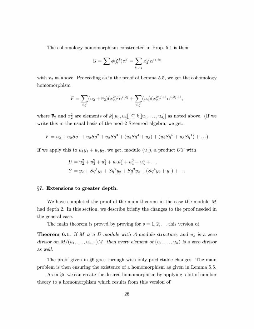
The cohomology homomorphism constructed in Prop. 5.1 is then

G =∑

φ(ξI)αI =∑i1,i2

xi22 αi1,i2

with x2 as above. Proceeding as in the proof of Lemma 5.5, we get the cohomology

homomorphism

F =∑i,j

(u2 + v2)(x22)jαi,2j +

∑i,j

(u4)(x22)j+1αi,2j+1,

where v2 and x22 are elements of k[[u3, u4]] ⊆ k[[u1, . . . , u4]] as noted above. (If we

write this in the usual basis of the mod-2 Steenrod algebra, we get:

F = u2 + u2Sq1 + u2Sq

2 + u2Sq3 + (u2Sq

4 + u3) + (u2Sq5 + u3Sq

1) + . . .)

If we apply this to u1y1 + u2y2, we get, modulo (u1), a product UY with

U = u22 + u2

3 + u24 + u3u

24 + u3

4 + u44 + . . .

Y = y2 + Sq1y2 + Sq2y2 + Sq3y2 + (Sq4y2 + y1) + . . .

§7. Extensions to greater depth.

We have completed the proof of the main theorem in the case the module M

had depth 2. In this section, we describe briefly the changes to the proof needed in

the general case.

The main theorem is proved by proving for s = 1, 2, . . . this version of

Theorem 6.1. If M is a D-module with A-module structure, and us is a zero

divisor on M/(u1, . . . , us−1)M , then every element of (u1, . . . , un) is a zero divisor

as well.

The proof given in §6 goes through with only predictable changes. The main

problem is then ensuring the existence of a homomorphism as given in Lemma 5.5.

As in §5, we can create the desired homomorphism by applying a bit of number

theory to a homomorphism which results from this version of

26

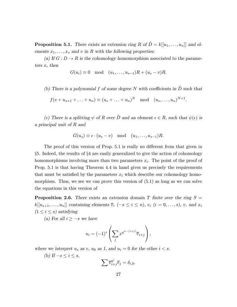
Proposition 5.1. There exists an extension ring R of D = k[[u1, . . . , un]] and el-

ements x1, . . . , xs and v in R with the following properties:

(a) If G : D → R is the cohomology homomorphism associated to the parame-

ters xi then

G(ui) ≡ 0 mod (u1, . . . , us−1)R+ (us − v)R.

(b) There is a polynomial f of some degree N with coefficients in D such that

f(v + us+1 + . . .+ un) ≡ (us + . . .+ un)N mod (us, . . . , un)N+1.

(c) There is a splitting ψ of R over D and an element ε ∈ R, such that ψ(ε) is

a principal unit of R and

G(us) ≡ ε · (us − v) mod (u1, . . . , us−1)R.

The proof of this version of Prop. 5.1 is really no different from that given in

§5. Indeed, the results of §4 are easily generalized to give the action of cohomology

homomorphisms involving more than two parameters xi. The point of the proof of

Prop. 5.1 is that having Theorem 4.4 in hand gives us precisely the requirements

that must be satisfied by the parameters xi which describe our cohomology homo-

morphism. Thus, we see we can prove this version of (5.1) as long as we can solve

the equations in this version of

Proposition 2.6. There exists an extension domain T finite over the ring S =

k[[us+1, . . . , un]] containing elements vi (−s ≤ i ≤ n), ei (i = 0, . . . , s), v, and xi

(1 ≤ i ≤ s) satisfying

(a) For all i ≥ −s we have

ui = (−1)i

∑j

xqn−(i+j)

vi+j

,

where we interpret us as v, u0 as 1, and ui = 0 for the other i < s.

(b) If −s ≤ i ≤ s, ∑vqj

i+jej = δi,0.

27

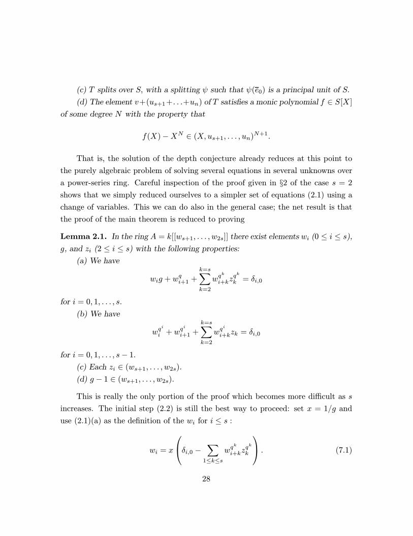
(c) T splits over S, with a splitting ψ such that ψ(e0) is a principal unit of S.

(d) The element v+(us+1+. . .+un) of T satisfies a monic polynomial f ∈ S[X]

of some degree N with the property that

f(X)−XN ∈ (X, us+1, . . . , un)N+1.

That is, the solution of the depth conjecture already reduces at this point to

the purely algebraic problem of solving several equations in several unknowns over

a power-series ring. Careful inspection of the proof given in §2 of the case s = 2

shows that we simply reduced ourselves to a simpler set of equations (2.1) using a

change of variables. This we can do also in the general case; the net result is that

the proof of the main theorem is reduced to proving

Lemma 2.1. In the ring A = k[[ws+1, . . . , w2s]] there exist elements wi (0 ≤ i ≤ s),g, and zi (2 ≤ i ≤ s) with the following properties:

(a) We have

wig + wqi+1 +k=s∑k=2

wqk

i+kzqk

k = δi,0

for i = 0, 1, . . . , s.

(b) We have

wqi

i + wqi

i+1 +k=s∑k=2

wqi

i+kzk = δi,0

for i = 0, 1, . . . , s− 1.

(c) Each zi ∈ (ws+1, . . . , w2s).

(d) g − 1 ∈ (ws+1, . . . , w2s).

This is really the only portion of the proof which becomes more difficult as s

increases. The initial step (2.2) is still the best way to proceed: set x = 1/g and

use (2.1)(a) as the definition of the wi for i ≤ s :

wi = x

δi,0 − ∑1≤k≤s

wqk

i+kzqk

k

. (7.1)

28

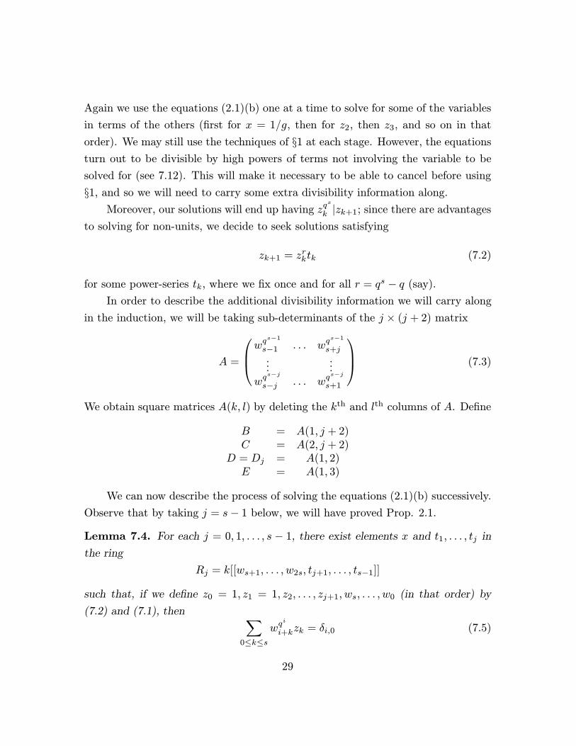
Again we use the equations (2.1)(b) one at a time to solve for some of the variables

in terms of the others (first for x = 1/g, then for z2, then z3, and so on in that

order). We may still use the techniques of §1 at each stage. However, the equations

turn out to be divisible by high powers of terms not involving the variable to be

solved for (see 7.12). This will make it necessary to be able to cancel before using

§1, and so we will need to carry some extra divisibility information along.

Moreover, our solutions will end up having zqs

k |zk+1; since there are advantages

to solving for non-units, we decide to seek solutions satisfying

zk+1 = zrktk (7.2)

for some power-series tk, where we fix once and for all r = qs − q (say).

In order to describe the additional divisibility information we will carry along

in the induction, we will be taking sub-determinants of the j × (j + 2) matrix

A =

wqs−1

s−1 . . . wqs−1

s+j

......

wqs−j

s−j . . . wqs−j

s+1

(7.3)

We obtain square matrices A(k, l) by deleting the kth and lth columns of A. Define

B = A(1, j + 2)C = A(2, j + 2)

D = Dj = A(1, 2)E = A(1, 3)

We can now describe the process of solving the equations (2.1)(b) successively.

Observe that by taking j = s− 1 below, we will have proved Prop. 2.1.

Lemma 7.4. For each j = 0, 1, . . . , s − 1, there exist elements x and t1, . . . , tj in

the ring

Rj = k[[ws+1, . . . , w2s, tj+1, . . . , ts−1]]

such that, if we define z0 = 1, z1 = 1, z2, . . . , zj+1, ws, . . . , w0 (in that order) by

(7.2) and (7.1), then ∑0≤k≤s

wqi

i+kzk = δi,0 (7.5)

29

holds for i = 0 and s− j ≤ i < s. Moreover, x′ = x−1 and t1 lie in (ws+1, . . . , w2s)

(as then do z2, z3, . . .). In addition

detDj |zj+1 (7.6)

Proof: We proceed by induction on j, and begin by proving this lemma when

j = 0. In this case, we seek only an x ∈ R0 making∑0≤k≤s

wkzk = 1 that is, (7.7)

w0 +w1 + w2t1 + w3(tr1t2) + . . .+ws(trs−2

1 · · · ts−1) = 1

Now, (7.1) shows that each wi ∈ (ws+1, . . . , w2s), except for w0 which is congruent

to x modulo (ws+1, . . . , w2s). Thus if we substitute (7.1) into (7.7) we obtain a

polynomial equation congruent to simply x ≡ 1. Therefore, x′ = x − 1 is to

satisfy a polynomial equation x′ = H(x′), where H ≡ 0 modulo (ws+1, . . . , w2s).

By Lemma 1.1, a solution exists, and has x′ ≡ 0, so that x ≡ 1. This proves the

lemma for j = 0 and so begins the induction.

Next we prove the inductive step, that is, we assume we have elements x and

t1, . . . , tj−1 in Rj−1 with detDj−1|zk so that (7.5) holds for i = 0 and i > s − j,and we find tj so that (7.5) also holds for i = s− j. This requires only that we can

find a tj ∈ Rj so that H = 0, where

F =∑

0≤k≤swq

s−j

s−j+kzk ∈ Rj−1 = Rj[[t]]. (7.8)

We need to examine the initial coefficients of tj in H and apply Lemma 1.3.

It is important to remember that we calculate H ∈ Rj−1 by substituting in the

assumed values of wi (i ≤ s), x, and ti (for i < j) in Rj−1; these values make the

appropriate equations (7.1) and (7.5) hold. All calculations that follow take place

in Rj−1 = Rj[[tj ]].

Lemma 7.9. (a) det(B) ≡ (−1)jxqs−jzqs

j det(D)q mod (zjtj)qs

(b) det(C) ≡ (−1)jxqs−jzqs

j det(E)q mod (zjtj)qs .

Proof: We prove (a); (b) is completely analogous.

30

For each k > 1, multiply the kth row from the bottom of B by (xzqk−1

k−1 )qs−j,

and add to the last row; naturally this doesn’t change the determinant but, in view

of (7.1), the lth entry of the bottom row has become

−x ∑j≤k≤s

zqk

k wqk

s+l−j+k

qs−j

≡ −xqs−jzqs

j wqs

s+l mod (zjtj)qs .

(The congruence follows from the definition (7.2).) Pull out the powers of x and zj

and move the bottom row to the top, and you obtain the matrix (D)q. The result

then follows. //

Lemma 7.10. det(B)+det(C) ≡ (−1)j(zj+1 detDj−H detDj−1) mod (zr2

j trj ).

Proof: B and C agree except in the first column, so detB + detC = detF, where

Fk,l = Rk,l for l > 1 and Fk,1 = Rk,1 +Ck,1. Multiply the lth column of F by zl (for

l > 1) and add to the first column. Since (7.5) holds for i > s− j, the kth entry of

the new first column is in most cases

−∑

j+1≤l≤szlw

qs−k

s+l−k. (7.11)

This is congruent to zj+1wqs−k

s+j+1−k modulo (zj+2, zj+3, . . .) ⊆ (zrj+1) ⊆ zr2

j trj (by

using (7.2)). However, when k = j, we cannot yet use (7.5); using (7.8) instead, we

see (7.11) must be increased by H in that single entry.

Now move the first column to the last and use the linearity of the determinant

in that column to get the desired result. //

We observe Dj−1 is non-singular. Indeed, it is clear from (7.3) that when re-

duced modulo (ws+2, . . . , w2s), D is lower-triangular, and indeed has a determinant

congruent to a power of ws+1 6≡ 0. Therefore, our goal of choosing a tj to make

H = 0 is equivalent to finding a tj to make H · detDj−1 = 0. In view of Lemmas

7.9 and 7.10 and definition (7.2), this is an equation of the form

xqs−jzqs

j (detD + detE)q − zrj tj detD + . . . = 0, (7.12)

31

where the deleted material lies in (zqs

j trj). In particular, (7.12) is divisible by zrj ;

dividing, we get an equation H ′ = 0, where H ′ ∈ Rj−1 = Rj [[tj]] is a power series

in tj whose initial coefficients are{H ′0 ≡ xq

s−jzqj(detD + detE)q

H ′1 ≡ detD(7.13)

modulo zqj . (The overlining here means this: view x, zj , detD, and detE also as

power series in tj and let x, etc., be the corresponding coefficients of t0j .)

Lemma 7.14. detD divides zjdetE.

Proof: The inductive hypothesis of Lemma (7.4) includes the statement that

detDj−1|zj in Rj−1; substitute tj = 0 in this and conclude detDj−1|zj . Thus,

we need only show (detE)(detDj−1) is a multiple of detDj .

Let (h1, . . . , hj−1) be the first row of the adjoint matrix of Dj−1. Thus,

(h1, . . . , hj−1) ·Dj−1 = (detDj−1, 0, . . . , 0). Consequently

(h1, . . . , hj−1, 0) ·A = (a, b, detDj=1, 0, . . . , 0, c) (7.15)

for some a, b, c ∈ Rj−1. Append the right-hand side of (7.15) as a top row of A and

delete the first column to get a (j + 1) × (j + 1) matrix we will call G. Observe

G is singular by construction, so if we expand detG along the first row, we get an

equation

0 = b · detDj−1 − (detDj−1) · E + (−1)jc · detB. (7.16)

In view of (7.9)(a), if we read (7.16) modulo tj , we conclude detDj divides

(detDj−1)(detE), as desired. //

Continuing then our discussion of (7.12), we see from equation (7.13) and

Lemma 7.14 that (7.12) is a power-series equation H ′(tj) = 0 with coefficients

H ′0, H′1, . . . such that (H ′1)q|H ′0. Therefore, we may apply Lemma 1.3 to conclude

that for some tj ∈ Rj−1 we indeed have H ′(tj) = 0; moreover,

tj ∼ zqj(detD)q−1(1 + (detE/detD)q) ∈ Rj . (7.17)

32

To complete the proof of the inductive step of Lemma 7.4, we must finally show

detDj |zj+1. Express detDj ∈ Rj−1 as a power series

detDj = detDj +∑k≥1

dktkj

with each dk ∈ Rj. Substituting in our newfound value of tj ∈ Rj, we conclude

from (7.17) that detDj ∼ detDj ∈ Rj , so that (again from (7.17)) detDj |tj . In

view of (7.2), this is sufficient.

In the special case j = 1, we are asked also to show t1 ∈ (ws+1, . . . , w2s). This

too is clear from (7.7), as D1 is the 1× 1 matrix (wqs−1

s+1 ).

So the inductive step is complete, and Lemma 7.4 is proven. //

Taking j = s − 1 in Lemma 7.4 completes the proof of Prop. 2.1. Then, as

indicated at the beginning of this section, we may modify the rest of the proof of

the main theorem given in §§1–6 so that it applies as well to all s as it does to s = 2.

33

References

[AH] M. F. Atiyah and F. Hirzebruch, Cohomologie-Operationen und Charak-

terische Klassen, Math. Zeit. 77 (1961) 149-187

[CA] H. Matsumura, Commutative Algebra, Benjamin/Cummings, Reading,

Mass. 1980

[D] L. E. Dickson, A Fundamental System of Invariants of the General Modular

Linear Group with a Solution of the Form Problem, Trans AMS 12 (1911) 75-98

[LS] P. Landweber and R. Stong, The Depth of Rings of Invariants over Finite

Fields, Proc. New York Number Theory Seminar, 1984, Springer Lect. Notes 1240

(1987)

[LSD] R. Stong, letter to P. Landweber, 5 May 1985, concluding several letters

on the Dickson algebra

[M] J. Milnor, The Steenrod Algebra and its Dual, Ann. Math. 94 (1971)

549-602

[R] D. Rector, Noetherian Cohomology Rings and Finite Loop Spaces with

Torsion, J. Pure Appl. Algebra, 32 (1984) 191-217

[W] C. Wilkerson, A Primer on the Dickson Invariants, Proc. Northwestern

Homotopy Theory Conference, Contemp. Math. 19, AMS (1983)

34