arX

iv:m

ath/

0202

288v

1 [

mat

h.A

G]

27

Feb

2002 On the Cohomology of Stable Map Spaces

K. Behrend and A. O’Halloran

February 26, 2002

Abstract

We describe an approach to calculating the cohomology rings of stablemap spaces M0,0(P

n, d).

Contents

1 Outline of the Method 71.1 Equivariant vector fields . . . . . . . . . . . . . . . . . . . . . . . 8

The Koszul complex . . . . . . . . . . . . . . . . . . . . . . . . . 91.2 Equivariant actions on vector bundles . . . . . . . . . . . . . . . 11

Actions of vector fields on vector bundles . . . . . . . . . . . . . 11The equivariant case . . . . . . . . . . . . . . . . . . . . . . . . . 14

1.3 Chern classes . . . . . . . . . . . . . . . . . . . . . . . . . . . . . 151.4 Localization to the big cell . . . . . . . . . . . . . . . . . . . . . . 18

2 Preliminaries on stable maps 202.1 Stable maps to vector bundles . . . . . . . . . . . . . . . . . . . . 202.2 Stable maps to P∞ . . . . . . . . . . . . . . . . . . . . . . . . . . 21

3 Parameterizing stable maps to Pn 233.1 For every i a degree 1 map to P1 . . . . . . . . . . . . . . . . . . 233.2 A degree d map to P

1 . . . . . . . . . . . . . . . . . . . . . . . . 283.3 The universal situation . . . . . . . . . . . . . . . . . . . . . . . . 32

The action of the multiplicative group . . . . . . . . . . . . . . . 363.4 Maps to Pn . . . . . . . . . . . . . . . . . . . . . . . . . . . . . . 373.5 The degree 2 case . . . . . . . . . . . . . . . . . . . . . . . . . . . 40

4 The vector field 414.1 Some deformation theory . . . . . . . . . . . . . . . . . . . . . . 414.2 The degree 3 case . . . . . . . . . . . . . . . . . . . . . . . . . . . 444.3 Chern classes . . . . . . . . . . . . . . . . . . . . . . . . . . . . . 494.4 The cohomology of M0,0(P∞, 3) . . . . . . . . . . . . . . . . . . . 524.5 A conjectural presentation for finite n . . . . . . . . . . . . . . . 554.6 The degree 2 case . . . . . . . . . . . . . . . . . . . . . . . . . . . 57

1

Introduction

Spaces of stable maps have enjoyed a lot of interest in recent years. They werefirst introduced by Kontsevich in 1994 (see [13]), and have since proven to bevery useful in many contexts, especially in Quantum Cohomology and MirrorSymmetry. Stable map spaces are natural completions of spaces of morphismsfrom algebraic curves to a fixed (non-singular complete) variety X . They ariseas natural generalizations of the moduli spaces of stable curves discovered byDeligne and Mumford [8].

Here we shall be mostly concerned with the spaces

M0,0(Pn, d) .

The generic member of M0,0(Pn, d) (at least if n ≥ 3) is a non-singular rationalcurve of degree d in projective n-space and, in fact, M0,0(Pn, d) is a compacti-fication of the space of all such curves, and thus has dimension dn+ d+ n− 3.The degenerations we allow at the boundary are pairs (C, f), where C is a nodalcurve of arithmetic genus 0 and f is a morphism f : C → Pn of degree d, suchthat every component of C which is contracted to a point by f has at least 3nodes. This also gives the correct picture for n = 1, 2. For example, M0,0(P1, d)compactifies the space of degree d ramified covers of genus zero of the projectiveline. We also remark that M0,0(Pn, 1) is simply the Grassmannian G(2, n+ 1)of lines in Pn.

The true beauty of the spaces M0,0(Pn, d) only becomes apparent if weconsider them as stacks. In fact, the algebraic stacks underlying the variousM0,0(Pn, d) are smooth and admit universal families. These are properties thatthe spaces M0,0(Pn, d) generally lack. We shall always work with these stacksand thus use the notation M0,0(Pn, d) for the stack of stable maps of degree dto Pn (of genus 0 without marked points).

Our goal is to compute the cohomology ring of M0,0(Pn, d), or at least, tooutline an approach by which this might be achieved. (The only previous resultin this direction is the computation of the Betti numbers of M0,ν(Pn, d) due toGetzler and Pandharipande [9].) Our method is inspired by the utility of C∗-actions for studying integrals over stable map spaces, but there is an additionalingredient: a vector field (which is compatible with the C∗-action).

This method is due to Akildiz and Carrell [1] and can be summarized asfollows. Let X be a non-singular projective variety over C with a C∗-actionand suppose that V is a vector field on X , satisfying λV = λV , for all λ ∈ C

∗

(we say that V is equivariant). If V has exactly one fixed point and Z is thescheme-theoretic fixed locus of V (so Z is a one-point non-reduced scheme),then we have

H∗(X,C) = Γ(Z,OZ) .

(See Examples 1.3 and 1.7, below, where this is worked out for the special caseof X = Pn. See also Remark 4.30, for the case of the Grassmannian of lines inPn.)

2

Our use of the method of Akildiz-Carrell is novel in two aspects: we applyit to stacks, but more significantly, the fixed locus Z of the vector field Vhas positive dimension. Thus we have to replace the ring of global sectionsΓ(Z,OZ) by the hypercohomology ring H0(X,K•

V ), where K•

V is the Koszulcomplex defined by the vector field V .

There is one important difference between Γ(Z,OZ) and H0(X,K•

V ). Thering Γ(Z,OZ) can be computed entirely on the fixed locus Z, whereasH0(X,K•

V ) depends on an open neighborhood of Z in X . Thus, in the caseof positive-dimensional fixed locus Z, the localizing power of the method ismuch weaker.

The method is saved by a somewhat surprising phenomenon. We discoveredthat we can restrict our attention entirely to a certain open subset U of X , eventhough U does not cover the fixed locus Z completely. This open subset U isthe ‘big cell’ associated by Bia lynicki-Birula [5] to the C∗-action on X .

In the cases we consider here, it turns out that the canonical map

H∗(X,C) = H0(X,K•

V ) −→ H0(U,K•

V ) = Γ(U,OZ)

is, though not injective, injective in all relevant degrees. This means injectivein all degrees that contain a generator or a relation.

One of our main results is an explicit description of the big Bia lynicki-Birulacell of M0,0(Pn, d) as a vector bundle over M0,d (modulo an action of the sym-metric group Sd). Here M0,d is the space of stable curves of genus zero with dmarked points, which is comparatively well understood.

The case d = 3 is particularly simple and we focus on it in the latter part ofthe paper. If d = 3 then M0,d is just a point and so the Bia lynicki-Birula cellis simply an affine space A4n modulo an action of S3. We succeed in writingdown the vector field V in canonical coordinates on A4n. This leads at least toa conjectural description of the cohomology ring of M0,0(Pn, 3). The truth ofthis conjecture depends only on a certain purely algebraic statement, which weverified using Macaulay 2 [10] for n ≤ 5.

More interesting than the case of finite n is the case of the limit as n ap-proaches ∞. The cohomology ring of M0,0(Pn, d) stabilizes as n increases, sowe can define a ring which we call the cohomology ring of M0,0(P∞, d), eventhough this latter stack does not make sense.

We succeed in describing the cohomology ring of M0,0(P∞, 3) completelyusing generators and relations (Theorem 4.15). This is the main result of thepaper. It says

H∗(M0,0(P∞, 3),C

)= C[b, σ1, ρ, σ2, τ, σ3]/

((τ2 − ρσ2), τσ3, ρσ3

).

The generators can be expressed in terms of Chern classes of certain canonicalvector bundles on M0,0(P∞, 3). The degrees of b and σ1 are 1, the degrees ofρ, σ2 and τ are 2 and the degree of σ3 is 3, using algebraic degrees (where thefirst Chern class has degree 1). Thus the degrees of the relations are 4, 5 and5, respectively.

3

Thus, as a ring, HDR

(M0,0(P∞, 3)

)is reduced, of pure dimension 4 and

has two irreducible components, C[b, σ1, σ2, σ3] and C[b, σ1, ρ, σ2, τ ]/(τ2 − ρσ2),intersecting transversally along C[b, σ1, σ2].

The case d = 2 is special, as M0,2 is not defined. It is much easier than thecase d = 3 and we have complete results.

We briefly outline the structure of the paper.In Section 1 we describe the theory of equivariant vector fields and their

relation to de Rham cohomology. We verify that the results of Akildiz andCarrell which we require hold for stacks. We improve on existing treatments ofChern classes by proving that the Carrell-Lieberman class [7] is homogeneous(see Section 1.3). Hence the Carrell-Lieberman characteristic classes (and notjust their leading terms) are equal to the corresponding Chern classes.

Section 2 assembles a few facts about stable map stacks which we requirelater. We observe that if E is a convex vector bundle on the variety X , then thestack of stable maps to E is a vector bundle over the stack of stable maps toX . We prove that the cohomology of M0,ν(Pn, d) stabilized as n increases andwe define the cohomology ring of M0,ν(P∞, d). Moreover,this cohomology ringmaps surjectively onto the cohomology ring of M0,ν(Pn, d), for every finite n.

In Section 3 we describe the big Bia lynicki-Birula cell of M0,0(Pn, d) as avector bundle over [M0,d/Sd]. The most significant case is n = 1. Here thebig Bia lynicki-Birula cell consists of all stable maps which are unramified over∞ ∈ P1. In the general case, it consists of all stable maps which avoid thecodimension 2 plane 〈0, 0, ∗, . . . , ∗〉 and intersect the hyperplane 〈0, ∗, . . . , ∗〉transversally d times.

By changing the C∗-action on Pn, we can cover all of M0,0(Pn, d) with vectorbundles over M0,d, and so our results lead, at least in principle, to an explicitdescription of the stable map stacks M0,0(Pn, d) in terms of stable curve spacesM0,d.

Section 4 starts with a recipe to calculate our vector field on M0,0(Pn, d).

The key result is that the derivative of the universal map f : C → Pn induces an

isomorphism Γ(C, TC) → Γ(C, f∗TPn). The remainder of the section containsthe calculations for the cases d = 2 and d = 3.

Notation and Conventions

Throughout the paper we will work over the ground field C of complex numbers.All of our algebraic stacks will be of Deligne-Mumford type. This means

that the diagonal X → X ×X is unramified. Deligne-Mumford stacks X admitetale presentations U → X , where U is a scheme. We denote the stack quotientassociated to a G-variety X by [X/G].

Whenever we consider sheaves on a Deligne-Mumford stack X , it is under-stood that these are sheaves on the small etale site of X . Objects of this etalesite are thus etale morphisms U → X , where U is a scheme. The topology onthis site is defined in the same way as for the etale site of a scheme. Any vectorbundle E → X defines a sheaf of local sections on the etale site of X , which weoften identify with E.

4

Any cohomology group of a sheaf on X is understood to be the cohomologyof the etale site with values in the given sheaf, unless mentioned otherwise.

Stable maps

For an algebraic variety X (not necessarily proper), we denote by H2(X)+ thesemigroup (with 0) of group homomorphisms Pic(X) → Z, which take non-negative values on ample line bundles. This semigroup is a convenient set oflabels for the class of a stable map. Given a stable map (C, x, f) to X , it isof class β ∈ H2(X)+ if deg(f∗L) = β(L), for all L ∈ Pic(X). If X = Pn, weidentify H2(X)+ with Z≥0.

We denote by Mg,n(X, β) the stack of stable maps of class β from n-markedgenus g curves to X .

Group actions

If an algebraic group G acts on a smooth scheme or a smooth algebraic stackX , we will denote this action on the right. Assume given a right action of G onX and a lift of this action to a vector bundle E over X . Then for any g ∈ Gand any local section e ∈ Γ(Ug,E), we denote by ge the section of E over Ugiven by the formula

(ge)(x) = e(xg)g−1 . (1)

In other words, ge ∈ Γ(U,E) is defined to make the diagram

Eg // E

Ug //

ge

OO

Ug

e

OO

commute. In particular, (1) defines a left representation of G on the C-vectorspace Γ(X,E) of global sections of E.

Any action of G on X lifts naturally to the vector bundles OX , TX andΩX , and so we get induced representations of G on functions, vector fields anddifferential forms on X . Explicitly, if f ∈ Γ(X,OX) is a regular function on X ,then gf = g∗f , or (gf)(x) = f(xg), for all x ∈ X . If V ∈ Γ(X, TX) is a vectorfield on X , then gV is characterized by the formula

Dg(x)((gV )(x)

)= V (xg)

or more briefly by(Dg)(gV ) = g∗V .

(Here Dg : TX → g∗TX is the derivative of g : X → X .) If ω ∈ Γ(X,Ω) is adifferential form on X , then gω is given by

gω = dg(g∗ω) ,

5

or(gω)(x) = dg(x)

(ω(xg)

),

where dg : g∗ΩX → ΩX denotes the natural pullback homomorphism. Notethat for all g ∈ G we have

g〈ω, V 〉 = 〈gω, gV 〉 . (2)

If F is another vector bundle over X to which the G-action has been lifted,then we get induced G-actions also on the vector bundles Hom(E,F ) and E⊗F ,given by the formulas (φg)(eg) = φ(e)g and (e ⊗ f)g = eg ⊗ fg. On globalsections, this gives rise to G-representations by the formulas

(gφ)(ge) = g(φ(e)

)

andg(e⊗ f) = ge⊗ gf .

Finally, given a C-linear sheaf homomorphism Φ : E → F , we define gΦ by

(gΦ)(ge) = g(Φ(e)

),

for any local section e of E. This generalizes the definitions above if Φ is OX -linear and gives rise to a G-representation on the space of all C-linear sheafhomomorphisms from E to F . For example, the universal derivation d : OX →ΩX satisfies gd = d, for all g ∈ G (this follows easily from (2)). Note that,because of this, g∇, for a connection ∇ on E, is again a connection on E.

Whenever any kind of object A satisfies an equation gA = A, for all g ∈ G,then we refer to A as G-invariant.

The case of Gm

In many cases our group G will be equal to the multiplicative group Gm. If weare given a right Gm-action on a vector bundle E, lifting a right action of Gm onX , then we refer to this action as the geometric action, to distinguish it fromthe action of Gm on E by scalar multiplication on the fibers, which we shall callthe linear action. Of course the geometric and the linear action commute witheach other.

In this case the (geometric) Gm-action gives rise to a C∗-representation onall the above mentioned vector spaces, i.e., it makes them into graded C-vectorspaces. The homogeneous elements A of degree i satisfy

λA = λiA ,

for all λ ∈ C∗. Of particular interest to us are elements of degree one; we shallcall them Gm-equivariant, or just equivariant, since there is rarely any fear ofconfusion. In particular, this gives rise to the notion of equivariant vector field.

6

1 Outline of the Method

Let X be a smooth and proper Deligne-Mumford stack. Assume that

Hp(X,Ωq) = 0, for all p 6= q,

where Ω = ΩX is the sheaf of Kahler differentials on X . (See Remark 1.8.)We will be interested in the graded ring

HDR(X) =⊕

p

Hp(X,Ωp) .

The notation HDR(X) is justified, because under our assumption

⊕

p

Hp(X,Ωp) = H(X, (Ω•, d)

),

where (Ω•, d) is the algebraic de Rham complex of X . We use the algebraicgrading, i.e., we consider Hp(X,Ωp) to have degree p.

Remark 1.1 Let Xan be the (small) analytic site of X . By a theorem ofGrothendieck (see [11]) we have

H(U, (Ω•, d)

)= H(Uan,C),

for every smooth variety U . Choosing an etale presentation U → X , where Uis a smooth variety, we obtain E2-spectral sequences

Hq(Up, (Ω

•, d))⇒ H

p+q(X, (Ω•, d)

)

andHq(Up

an,C)⇒ Hp+q(Xan,C) ,

where Up is the (p+ 1)-fold fibered product of U with itself over X .Thus we conclude that

H(X, (Ω•, d)

)= H(Xan,C) .

Letting X be the coarse moduli space of X , we have

H(Xan,C) = H(Xan,C) ,

essentially because group cohomology of any finite group with values in C van-ishes. Thus we have

HDR(X) = H(Xan,C) = H(Xan,C) ,

and so we can also interpret our ringHDR(X) as the usual (singular) cohomologyring of the topological space underlying the variety X over C.

Note that for H(Xan,C) we also use the algebraic grading, i.e., we considerH2p(Xan,C) to have degree p.

7

1.1 Equivariant vector fields

Now assume that we are given a (right) Gm-action on X . Recall that we defineda vector field V on X to be Gm-equivariant if λV = λV , for all λ ∈ C∗. Notethat V is equivariant if and only if the diagram

λ∗ΩXλ∗V //

λdλ

λ∗OX

=

ΩX

V // OX

commutes, for all λ ∈ C∗.

Remark 1.2 Let G be the semidirect product of the multiplicative group andthe additive group, where the action of Gm by conjugation on Ga is given byscalar multiplication: λa = λa. We can identify G with the group of 2 × 2invertible matrices of the form

(1 0a λ

)

.

Suppose we are given a right action of G on X . Then restricting to the mul-tiplicative subgroup of G gives us a (right) action of Gm on X . Taking thederivative of the Ga-action on X defines a vector field V on X . More precisely,let

φx : A1 −→ X

a 7−→ xa

denote the orbit map of x ∈ X for the action of Ga. Then V (x) = Dφx(0),where we identify the linear map

Dφx(0) : TA1(0) −→ TX(x)

with the image of the canonical generator 1 ∈ TA1(0).Taking the derivative at 0 of the commutative diagram

A1

λ

φxλ // X

A1φx // X

λ

OO

proves that Dφxλ(0) = Dλ(x)Dφx(0)λ, and hence that λV (x) = λV (x). ThusV is Gm-equivariant. This is the most common source of Gm-equivariant vectorfields.

8

Example 1.3 Let Dλ denote the diagonal (n+1)× (n+1)-matrix with entries(1, λ, . . . , λn) along the diagonal. Let N denote the nilpotent (n+ 1)× (n+ 1)-matrix with ones along the sub-diagonal and zeros elsewhere. Then

(1 0a λ

)7−→ eaNDλ

defines a group homomorphism G → GL(n + 1). Via this homomorphism, wedefine a right action of G on Pn, by acting in the natural way on homogeneouscoordinate vectors of Pn, which we consider to be row vectors of length n+ 1.

As in Remark 1.2, we get an induced Gm-action and an equivariant vectorfield W on Pn. In standard homogeneous coordinates on Pn this vector field isgiven by

W =n∑

i=1

xi∂

∂xi−1.

The zero locus of this vector field consists of one point, namely the originin the standard affine space An ⊂ Pn defined by x0 = 1. In affine coordinatessi = xi

x0this vector field is given by

W = −s1sn∂

∂sn+n−1∑

i=1

(si+1 − s1si)∂

∂si.

(Recall the relation∑n

i=0 xi∂∂xi

= 0.)

The Koszul complex

Let X be as above, endowed with a Gm-action. Let V : ΩX → OX be anequivariant vector field on X . We can associate to V the Koszul complex

ΩNXι(V )−→ . . .

ι(V )−→ Ω2

X

ι(V )−→ ΩX

V−→ OX ,

where N denotes the dimension of X , hence the rank of ΩX , and ι(V ) denotescontraction with V . (If we pull back this Koszul complex to an etale and affineX-scheme over which we can trivialize ΩX , then the vector field V is given by Nregular functions and the above complex is the usual Koszul complex associatedto this sequence of regular functions.)

We set Kp = Ω−pX , for p ∈ Z, and denote the above Koszul complex by

K•

V =(K•, ι(V )

).

Note that K•

V is a sheaf of differential graded commutative (with unit) OX -algebras on X .

We are interested in the hypercohomology H(X,K•

V ), and its relation toHDR(X).

9

Lemma 1.4 For every p 6= 0 we have Hp(X,K•

V ) = 0. Moreover, H0(X,K•

V )is a commutative filtered C-algebra, and for the associated graded algebra wehave

gr H0(X,K•

V ) = HDR(X) .

Proof. This follows immediately from the standard E1 spectral sequence ofhypercohomology and our assumption on the vanishing of off-diagonal Hodgegroups.

For λ ∈ C∗ we define a homomorphism ψλ : λ∗K•

V → K•

V by

. . . // λ∗ΩpXλ∗ι(V ) //

λpdλ

. . . // λ∗ΩXλ∗V //

λdλ

λ∗OX

=

. . . // ΩpX

ι(V ) // . . . // ΩXV // OX

(3)

Here dλ : λ∗ΩpX → ΩpX is the homomorphism induced on the exterior power bythe derivative dλ : λ∗ΩX → ΩX . Note that ψλ is a homomorphism of differentialgraded algebras.

We can use ψλ to define a representation of C∗ on the hypercohomologyH0(X,K•

V ). We simply associate to λ ∈ C∗ the automorphism

H0(X,K•

V )λ∗

−→ H0(X,λ∗K•

V )ψλ−→ H

0(X,K•

V ) .

Thus H0(X,K•

V ) becomes a graded C-algebra.

Proposition 1.5 (Akildiz-Carrell [1]) There is a canonical isomorphism ofgraded C-algebras

H0(X,K•

V ) = HDR(X) .

Proof. Note that the grading induced by the C∗-representation on H0(X,K•

V )is compatible with the filtration induced by the E1-spectral sequence. Thuswe get an induced C∗-representation on the associated graded algebra. Oneshows that via this induced representation, C∗ acts on Hp(X,Ωp) through thecharacter λ 7→ λp. Then the proof is finished, in view of the lemma from linearalgebra which we state below.

For the convenience of the reader, we recall the proof that C∗ acts on

Hp(X,Ωp) through λ 7→ λp. One simply factors ψλ as ψλ = φλ dλ, whereφλ is multiplication by λp on Ωp. Thus the action of λ ∈ C∗ on Hp(X,Ωp)factors as ψλ λ∗ = φλ (dλ λ∗). Now dλ λ∗ is the homomorphism on deRham cohomology induced by the morphism λ : X → X , which is the identity.On the other hand, φλ obviously induces multiplication by λp on Hp(X,Ωp).

10

Lemma 1.6 Let H be a commutative filtered C-algebra with a C∗-representation, respecting the filtered algebra structure. Denote the filtrationby

. . . ⊂ Fi−1 ⊂ Fi ⊂ . . .

Suppose that C∗ acts on Fi/Fi−1 through λ 7→ λi. Let H =⊕

j Hj be the gradinginduced by the C∗-representation, where Hj is the eigenspace of the characterλ 7→ λj . Then for all i we have Fi =

⊕j≤iHj, so that we have

H = grH ,

as graded algebras. Here the grading on H comes from the C∗-representation,and the grading on grH from the filtration on H.

Example 1.7 Consider the Gm-action and equivariant vector field W on Pn

of Example 1.3. Then, because the zero locus Z of V has dimension zero, theKoszul complex K•

W is a resolution of OZ , and so we have that

H0(Pn,K•

W ) = Γ(Z,OZ)

= C[s1, . . . , sn]/(−s1sn, s2 − s21, s3 − s1s2, . . . , sn − s1sn−1)

= C[s1]/(−sn+11 ) .

Note how the latter relations serve to recursively eliminate s2, . . . , sn, leavingonly the first generator s1 and the first relation −s1sn.

Remark 1.8 The assumption that Hp(X,Ωq) = 0, for all p 6= q, was madelargely for simplicity, and because it is satisfied in all cases considered in thispaper. It seems likely that the E1-spectral sequence abutting to H(X,K•

V )always degenerates. (See [6], where this is proved for the case of a compactKahler manifold X and a vector field V with non-empty zero set). If thisis the case, then H∗(X,K•

V ) is a doubly graded C-algebra and isomorphic toHDR(X) =

⊕p,qH

p(X,Ωq) as such.

1.2 Equivariant actions on vector bundles

To understand Chern classes in the context of Proposition 1.5, we need to studyactions of vector fields on vector bundles. First we recall this concept withoutthe presence of a Gm-action. Then we consider the Gm-equivariant case.

Actions of vector fields on vector bundles

Let X be a smooth Deligne-Mumford stack and E a vector bundle on X .

Definition 1.9 (Carrell-Lieberman [7]) Let V be a vector field on X . Anaction of V on E is a homomorphism of sheaves of C-vector spaces

V : E −→ E ,

11

satisfying the Leibniz rule

V (fe) = V (f)e+ fV (e) ,

for all local sections f of OX and e of E. Here we interpret V as a C-linearderivation V : OX → OX .

Note that any two actions of V on E differ by a homomorphism of vectorbundles E → E.

Remark 1.10 An action V of V on E is the same thing as a Gm-invariant vectorfield V on E lifting the vector field V on X . Here we mean Gm-invariant withrespect to the natural fiber-wise action of Gm on E by scalar multiplication.This means that in local (linear) coordinates on E, the coefficients of V arelinear in these ‘vertical’ coordinates.

The action V is given in terms of the invariant lift V by

V (e) = De(V )− e∗(V ) ,

for any local section e : X → E. This is an equality of sections of e∗TE . Thebundle e∗TE fits into the short exact sequence

0 −→ E −→ e∗TE −→ TX −→ 0 ,

which is canonically split by De : TX → e∗TE . We will often identify theinvariant lift V and the action V .

If the vector field V on X comes about by differentiating a Ga-action, andthe vector field V on E comes about by differentiating a compatible linear Ga-action on E, then V is Gm-invariant, and therefore gives rise to an action of Von E.

Examples 1.11 1. Let ∇ : E → ΩX ⊗ E be a connection on E. Then, via ∇,every vector field V acts on E. Just set V equal to the covariant derivative ∇V .

2. Given the vector field V on X , the vector bundles OX , TX and ΩX havenatural V -actions. For OX , we have V = V , for TX , we have that V is equal tothe Lie derivative with respect to V and for ΩX we have V = d V .

3. Given actions of V on the vector bundles E and F , there are naturalinduced actions on E⊗F and Hom(E,F ). These are given by the usual Leibnizformulas

V (e⊗ f) = V (e)⊗ f + e⊗ V (f)

V (φ)(e) = V(φ(e)

)− φ

(V (e)

).

4. Consider the vector field W on Pn from Example 1.3. It acts on O(1) bythe formula

W (xi) =

xi+1 if i < n

0 if i = n .

We get induced actions of W on O(m), for all m ∈ Z.

12

Remark 1.12 Recall how connections on E can be described in terms of split-tings of the short exact sequence of OX -modules (the Atiyah extension)

0 −→ ΩX ⊗ E −→ At(E) −→ E −→ 0 , (4)

where At(E) is the OX -module whose underlying sheaf of C-vector spaces isequal to E ⊕ (Ω⊗ E) and whose OX -module structure is defined by

f ∗ (e, ω ⊗ e′) = (fe, fω ⊗ e′ + df ⊗ e) .

If we denote by s0 the C-linear splitting of (4) given by e 7→ (e, 0), then everyOX -linear splitting s of (4) defines a connection on E by the formula s = s0 +∇,and conversely, every OX -linear splitting of (4) comes from a unique connectionon E in this way.

We can describe actions of V on E in a similar vein. We define a short exactsequence of OX -modules

0 −→ E −→ AtV (E) −→ E −→ 0 , (5)

where AtV (E) is the OX -module whose underlying sheaf of C-vector spaces isE ⊕ E and whose OX -modules structure is given by

f ∗ (e, e′) = (fe, fe′ + V (f)e) .

Moreover, the inclusion in (5) is given by e′ 7→ (0, e′) and the quotient map by(e, e′) 7→ e. Again, let us denote the C-linear splitting e 7→ (e, 0) of (5) by s0.Then actions of V on E and OX -linear splittings of (5) correspond bijectively

to each other via the formula s = s0 + V .Note that pushing out (4) via the OX -homomorphism V ⊗idE : ΩX⊗E → E

gives (5). In other words, we have a homomorphism of short exact sequences ofOX -modules

0 // ΩX ⊗ E

V⊗id

// At(E)

// E

id

// 0

0 // E // AtV (E) // E // 0 .

(6)

Thus every action V of V on E gives rise to an OX -linear map (the Carrell-Lieberman map)

CL(V ) : At(E) −→ E (7)

(e, ω ⊗ e′) 7−→ 〈ω, V 〉e′ − V (e) ,

making the diagram

ΩX ⊗ E

V⊗id

// At(E)

CL(V )yyssssssssss

E

commute.

13

The equivariant case

Now suppose that X is endowed with a Gm-action, which has been lifted to anaction of Gm on E by linear isomorphisms. Given a vector field V on X , and anaction V of V on E, then λV is an action of λV on E. So if V is equivariant, itis natural to consider equivariant lifts V , which satisfy λV = λV .

Remark Let V be an invariant vector field on E (with respect to the linear

action), lifting the vector field V on X . Let V be the associated action of V onE. Then V is equivariant as a vector field on E (with respect to the geometric

action) if and only if V is equivariant as a C-linear homomorphism from E toE.

Hence, if the Gm-action and the equivariant vector field V on X come froman action of the group G on X as in Remark 1.2, then any lift of the G-actionto a vector bundle E over X gives rise to an equivariant action of V on E.

If V and V ′ are two equivariant actions of V on E, then the differenceh = V − V ′ is an equivariant homomorphism.

Example 1.13 If ∇ is an invariant connection on E, and V an equivariantvector field on X , then the covariant derivative ∇V is an equivariant action ofV on E.

Example 1.14 Suppose that E is trivial and that there exists a trivializationof E by a basis of global sections (ei), which are homogeneous, i.e., we have

λei = λriei ,

for all i and certain integers ri, with respect to the geometric Gm-action. Thenthe connection on E induced by this trivialization via the formula ∇(ei) = 0is invariant, and hence the covariant derivative with respect to an equivariantvector field is equivariant.

Example 1.15 Consider the Gm-action on Pn from Example 1.3. It lifts natu-rally to O(1) by the formula

λxi = λixi .

The action W of W on O(1) given by W (xi) = xi+1 (xn+1 = 0) is equivariantwith respect to this Gm-action. The same is true for the induced actions onO(m), for all m ∈ Z.

Remark 1.16 Considering the natural induced action of Gm on the short exactsequence (4), we note that all maps in (4) are Gm-invariant, and that invariantsplittings correspond to invariant connections.

Denote by E(−1) the vector bundle E with the geometric Gm-action modifiedby the linear Gm-action in such a way that λ(e(−1)) = λλe, where we have

14

denoted by e(−1) the section e of E considered as a section of E(−1). Weintroduce the Gm-action on (5) indicated by

0 −→ E −→ E(−1) ⊕ E −→ E(−1) −→ 0 .

This choice of Gm-action is necessary to ensure that the formula

λ(f ∗ (e, e′)

)= (λf) ∗ λ(e, e′)

holds, for the OX -action on AtV (E).Now invariant splittings of (5) correspond to equivariant actions of V on E.

Moreover, the homomorphism of short exact sequences (6) is of degree one (or

equivariant, in our language). The homomorphism CL(V ) : At(E) → E given

by an equivariant action of V on E is equivariant: λ(CL(V )

)= λCL(V ).

For future reference, we need some facts about the functorial behavior ofequivariant actions on vector bundles.

Lemma 1.17 (pullbacks) Let f : X → Y be a morphism of smooth Deligne-Mumford stacks. Let E be a vector bundle over Y . Assume that Gm acts com-patibly on X, Y and E. Let V be an equivariant vector field on X and W anequivariant vector field on Y , such that Df(V ) = W . Let W be an equivariant

action of W on E. Then there is an induced equivariant action V of V on f∗E,such that

V(f∗(e)

)= f∗

(W (e)

),

for every local section e of E. If V , W and W come from compatible actions ofG on X, Y and E, then V comes from the induced G-action on f∗E.

Lemma 1.18 (pushforward) Let π : X → Y be a flat and proper morphismof smooth Deligne-Mumford stacks. Let E be a vector bundle on X, such thatπ∗E is a vector bundle on Y . Assume that Gm acts compatibly on X, Y and E.Let V be an equivariant vector field on X and W an equivariant vector field onY , such that Dπ(V ) = W . Let V be an equivariant action of V on E. Then

there is an induced equivariant action W of W on π∗E, such that

W (e) = V (e) ,

for every local section e of π∗E. If V , W and V come from compatible actionsof G on X, Y and E, then W comes from the induced G-action on π∗E.

1.3 Chern classes

Now suppose that X is a smooth Deligne-Mumford stack and E a vector bundleon X of rank r. Suppose given compatible Gm-actions on X and E. Finally, letV be an equivariant vector field on X .

15

We shall now tensor the Koszul complex K•

V over OX with the sheaf of OX -modules Hom(E,E). Thus K•

V ⊗ Hom(E,E) is a sheaf of differential gradedmodules over the sheaf of differential gradedOX -algebras K•

V . Hence the hyper-cohomology H0

(X,K•

V⊗Hom(E,E))

is a module over the C-algebra H0(X,K•

V ).

A C∗-representation on H0(X,K•

V ⊗Hom(E,E))

is given by the composition

H0(X,K•

V ⊗Hom(E,E)) λ∗

−→ H0(X,λ∗K•

V ⊗ λ∗Hom(E,E)

)

ψλ⊗ρ−→ H

0(X,K•

V ⊗Hom(E,E)),

where ψλ is the homomorphism given by (3) and ρ : λ∗Hom(E,E) →Hom(E,E) is the natural isomorphism induced by the isomorphism λ∗E ∼= Egiven by the (geometric) action of Gm on E.

Note that the C∗ action on H0(X,K•

V ⊗Hom(E,E))

is compatible with the

H0(X,K•

V )-action. Thus, via this C∗-representation, H0(X,K•

V ⊗Hom(E,E))

becomes a graded module over the graded C-algebra H0(X,K•

V ).

Now let V be an equivariant action of V on E. The Carrell-Liebermanhomomorphism CL(V ) of (7) gives rise to a homomorphism of complexes

. . . // 0

// ΩX ⊗ E

id

// At(E)

CL(V )

// 0

. . . // Ω2X ⊗ E

// Ω⊗ EV⊗id // E // 0

which we can view as a homomorphism in the derived category from E toK•

V ⊗ E, because [ΩX ⊗ E → At(E)] is a resolution of E. We denote thishomomorphism by

cV (E) ∈ HomD(OX)(E,K•

V ⊗ E) .

Via the canonical identification

HomD(OX)(E,K•

V ⊗ E) = H0(X,K•

V ⊗Hom(E,E)),

cV (E) gives rise to a hypercohomology class, which we shall also denote by

cV (E) ∈ H0(X,K•

V ⊗Hom(E,E))

and call the Carrell-Lieberman class.It follows directly from Remark 1.16 that the Carrell-Lieberman class cV (E)

is a degree one element of H0(X,K•

V ⊗Hom(E,E)).

Now assume given a regular function Q : M(r × r)→ A1 of degree p, whichis invariant under conjugation. This function gives rise to a morphism of X-schemes

QE : Hom(E,E) −→ OX ,

by associating to an endomorphism φ of E the number we get by applyingQ to any matrix representation of φ. The X-morphism QE corresponds to

16

a morphism of OX -algebras OX [t] → SymHom(E,E)∨, where t is a coordi-nate on A1. Evaluating at t, this morphism gives rise to a global section ofSympHom(E,E)∨, or equivalently, a symmetric p-linear homomorphism

Q′ : SympHom(E,E) −→ OX .

If φ is a local section of Hom(E,E), then the regular function QE φ on X isequal to Q′(φp).

Recall how characteristic classes are defined in terms of the Atiyah class. TheAtiyah class c(E) ∈ H1

(X,Ω⊗Hom(E,E)

)is the cohomology class correspond-

ing to the extension of OX -modules At(E) given by (4) under the identification

Ext1(E,ΩX ⊗ E) = H1(X,ΩX ⊗Hom(E,E)

).

It gives rise to an element

c(E)∪p ∈ Hp(X,Ω⊗p ⊗Hom(E,E)⊗p

),

by taking cup products. Then we apply the map induced on Hp by the compo-sition

Ω⊗p ⊗Hom(E,E)⊗p −→ Ωp ⊗ SympHom(E,E)id⊗Q′

−→ Ωp ⊗OX = Ωp

to c(E)∪p. We obtain cQ(E) ∈ Hp(X,Ωp), the characteristic class of E definedby Q:

cQ(E) = Hp(id⊗Q′)(c(E)∪p

).

For example, if Q is (−1)p times the degree r − p coefficient of the charac-teristic polynomial, then cQ(E) is the p-th Chern class of E.

Remark If X is a scheme, then under our identification of Hp(X,Ωp) withthe singular cohomology Hp(X,C), these Chern classes correspond to the usualChern classes.

Let us now apply a corresponding process to the Carrell-Lieberman classcV (E). We start by taking the cup product of this class with itself p times:

cV (E)∪p ∈ H0(X, (K•

V )⊗p ⊗Hom(E,E)⊗p).

Then we compose with the map induced on H0 by

(K•

V )⊗p ⊗Hom(E,E)⊗pµ⊗Q′

−→ K•

V ⊗OX = K•

V ,

where µ : (K•

V )⊗p → K•

V is the multiplication map induced from the algebrastructure on K•

V . Thus we get the associated characteristic class

cQV

(E) = H0(µ⊗Q′)

(cV (E)∪p

)∈ H

0(X,K•

V ) . (8)

17

Proposition 1.19 The class cQV

(E) ∈ H0(X,K•

V ) is homogeneous of degree

degree p. If X is proper and satisfies hij(X) = 0, for all i 6= j, then under theidentification of Proposition 1.5 we have

cQV

(E) = cQ(E) .

Proof. Let us denote by K>−1V the naıve cutoff of K•

V at minus one. So

K>−1V denotes the two term complex [ΩX → OX ] given by the vector field V .

There is a canonical injection of complexes K>−1V → K•

V , which also gives rise

to an injection K>−1V ⊗ E → K•

V ⊗ E. We also have a canonical projection

K>−1V → ΩX [1], giving rise to K>−1

V ⊗E → ΩX ⊗E[1]. In the derived category,we get an induced diagram

HomD(OX)(E,K>−1V ⊗ E)

// HomD(OX)(E,K•

V ⊗ E)

HomD(OX)(E,ΩX ⊗ E[1])

which we identify with the diagram

HomD(OX)(E,K>−1V ⊗ E)

// H0(X,K•

V ⊗Hom(E,E))

H1(X,ΩX ⊗Hom(E,E)

)

Directly from the construction, it follows that the Carrell-Lieberman class cV (E)

lifts to HomD(OX )(E,K>−1V ⊗ E), and this lift maps to the Atiyah class:

CL(V )_

// cV (E)

c(E)

The claim follows.

1.4 Localization to the big cell

Let X be, as above, a smooth Deligne-Mumford stack with a Gm-action, andlet E be a vector bundle to which the Gm-action has been lifted. Let V be anequivariant vector field on X and V an equivariant action of V on E. Finally,let us denote by Z ⊂ X the closed substack defined by the vanishing of V :the structure sheaf OZ of Z is defined to be the cokernel of the vector fieldV : ΩX → OX . Another way to think of OZ is as the zero-degree cohomologysheaf of K•

V .

18

There is a canonical morphism of sheaves of differential graded algebrasK•

V → OZ , inducing a canonical morphism of graded algebras

H0(X,K•

V ) −→ Γ(Z,OZ) .

Remark When we restrict to Z, the action V induces an OZ -linear homomor-phism VZ : EZ → EZ . Applying the invariant polynomial Q, we get a regularfunction

Q(VZ) ∈ Γ(Z,OZ) .

Under the canonical morphism H0(X,K•

V )→ Γ(Z,OZ) the characteristic class

cQV

(E) maps to Q(VZ).

If X is affine and E is trivial over X , trivialized by a homogeneous basis (ei)

as in Example 1.14, then we form the matrix M of V with respect to this basis.In other words, M = (mij) is a square matrix with entries mij ∈ Γ(X,OX),characterized by

V (ei) =∑

j

mjiej .

In this case we have

Γ(Z,OZ) = Γ(X,OX)/V(Γ(X,ΩX)

)

and we can compute Q(VZ) ∈ Γ(Z,OZ) simply as the congruence class ofQ(M) ∈ Γ(X,OX).

Note that if ei is homogeneous of degree di, then mij is homogeneous ofdegree di − dj + 1.

Example Returning to Example 1.7, using the equivariant action W of W onO(m) of Example 1.15, we see that a basis for O(m) over x0 = 1 ⊂ P

n is given

by xm0 . We have W (xm0 ) = mx1

x0xm0 = ms1x

m0 in the notation of Example 1.7.

Thus the matrix of W with respect to this basis is ms1 and so the first Chernclass c1

(O(m)

)∈ H0(Pn,K•

W ) is equal to ms1.

We shall apply these ideas in the following context. The stack X will beproper, smooth and satisfy our assumption on the vanishing of off-diagonalHodge numbers. The stack X will be endowed with a Gm-action and severalequivariant vector bundles Ei. Moreover, X will have an equivariant vector fieldV on it, with natural equivariant lifts Vi to the various Ei. We will constructan affine scheme T , with a lift of the Gm-action to T and an etale morphismT → X . Over T we trivialize all Ei using homogeneous bases. Finally, wechoose a collection of invariant polynomials Qi of various degrees, giving rise tocharacteristic classes ci = cQi

i (Ei) ∈ HDR(X).We consider the natural morphism

HDR(X) = H0(X,K•

V ) −→ H0(T,K•

V ) = Γ(T,OT )/V(Γ(T,ΩT )

), (9)

19

and note that we can compute the images of ci under (9) as Qi(Mi), where Mi is

the matrix representation of Vi with respect to our homogeneous basis of Ei|T .In the cases we consider, it will turn out that the map (9) is injective in

sufficiently low degrees and that HDR(X) is generated (as a C-algebra) by theclasses ci.

2 Preliminaries on stable maps

2.1 Stable maps to vector bundles

Let X be a smooth and proper algebraic variety and E a vector bundle over X ,with structure morphism p : E → X .

Note Pulling back via p induces an isomorphism of Picard groups p∗ :Pic(X) → Pic(E) which preserves the ample line bundles. Hence we have acanonical isomorphism H2(E)+ → H2(X)+ which we use to identify these twosemi-groups.

Note Let f : C → E be a morphism from a prestable marked curve (C, x)

to E. Then f is stable of class β if and only if p(f) = p f is stable of class

β. This is because p(f) cannot contract any component of C which f does notalready contract, because no component of C can map into a fiber of p , thesefibers being affine.

Let

C

π

f // X

Mg,n(X, β)

be the universal curve and universal stable map. We may view π∗f∗E as a

(relative) scheme over Mg,n(X, β). Then it represents the following functor:

π∗f∗E(T ) = Γ(CT , f

∗E) ,

for any Mg,n(X, β)-scheme T . Here CT abbreviates the pull-back of C to T . IfT →Mg,n(X, β) is given by (C, x, f), then

π∗f∗E(T ) = Γ(C, f∗E)

= f : C → E | p(f) = f .

Hence π∗f∗E as a stack in its own right (forgetting the Mg,n(Xβ)-structure)

associates to the C-scheme T the groupoid of triples (C, x, f ), where (C, x) is a

prestable marked curve and f : C → E is a morphism such that p(f) : C → X

20

is a stable map of class β. by the above notes, this is equivalent to saying thatf is a stable map of class β. Thus we conclude that

π∗f∗E = Mg,n(E, β) .

In particular, Mg,n(E, β) is an algebraic stack, representable over Mg,n(X, β),by an (abelian) cone (see [3] for this terminology). We note the following con-sequence:

Proposition 2.1 If E is convex over X, i.e., H1(P1, f∗E) = 0 for all mor-phisms f : P1 → X, then M0,n(E, β) is a vector bundle over M0,n(X, β),canonically identified π∗f

∗E. The rank of this vector bundle is 〈c1(E), β〉+rkE.

Example 2.2 For m ≥ 0, the vector bundle Em = π∗f∗OPn(m) over

M0,ν(Pn, d) has rank md+ 1 and represents M0,ν(OPn(m), d).

2.2 Stable maps to P∞

Let n < m be integers and consider Pn as a subvariety of Pm via Pn =〈x0, . . . , xn, 0, . . . , 0〉 ⊂ Pm. Let H = 〈0, . . . , 0, xn+1, . . . , xm〉 ∼= Pm−n−1.Let U = Pm −H and consider the projection with center H onto Pn, which isdefined on U and makes U a vector bundle over Pn of rank m− n, in fact thisvector bundle is isomorphic to a direct sum of m− n copies of OPn(1).

By applying M0,ν( · , d) to the diagram of varieties

U

// Pm

Pn

we get the diagram of stacks

M0,ν(U, d)

ρ

ι // M0,ν(Pm, d)

M0,ν(Pn, d) .

Here ρ is a vector bundle of rank (d + 1)(m− n). Let κ be the zero section ofthis vector bundle. The projection ρ is a homotopy equivalence implying that

κ∗ : Hp(M0,ν(U, d)an,C

) ∼−→ Hp

(M0,ν(Pn, d)an,C

)

is an isomorphism for all p.The complement of M0,ν(U, d) in M0,ν(Pm, d) consists of all stable maps to

Pm whose image intersects H . The locus of these stable maps has codimensionn in M0,ν(Pm, d). Thus

ι∗ : Hp(M0,ν(Pm, d)an,C

)−→ Hp

(M0,ν(U, d)an,C

)

21

is an isomorphism for all p ≤ 2n− 2, by cohomological purity.We conclude that

(ικ)∗ : Hp(M0,ν(Pm, d)an,C

)−→ Hp

(M0,ν(Pn, d)an,C

)(10)

is an isomorphism for p ≤ 2n− 2. This leads to the following definition:

Definition 2.3 For every p ≥ 0 we define

Hp(M0,ν(P∞, d)an,C

)= Hp

(M0,ν(Pn, d)an,C

),

for any n such that n ≥ 12 (p+ 2).

It follows from the above considerations that any two different choices of nlead to canonically isomorphic definitions of Hp

(M0,ν(P∞, d)an,C

), for fixed p.

Taking the direct sum over all p gives rise to the C-algebra

H∗(M0,ν(P∞, d)an,C

).

For any n we have the canonical restriction map

H∗(M0,ν(P∞, d)an,C

)−→ H∗

(M0,ν(Pn, d)an,C

)

which is a C-algebra morphism and an isomorphism in degrees less than n (recallour degree convention from Remark 1.1).

Remark 2.4 For every ν, d, n we have

H∗(M0,ν(Pn, d)an,C

)= HDR

(M0,ν(Pn, d)

)=⊕

p

Hp(M0,ν(Pn, d),Ωp

).

The first equality follows from Remark 1.1. The second equality is proved usingthe technique of virtual Hodge polynomials to reduce to the strata of a suitablestratification. Use the stratification by topological type. The details are workedout by Getzler and Pandharipande in [9]. This justifies writing also

H∗(M0,ν(P∞, d)an,C

)= HDR

(M0,ν(P∞, d)

)=⊕

p

Hp(M0,ν(P∞, d),Ωp

).

Remark 2.5 It is, in fact, true that

(ικ)∗ : Hp(M0,ν(Pm, d)an,C

)−→ Hp

(M0,ν(Pn, d)an,C

)

is surjective for all p. One way to prove this is as follows. Consider the Gm-actionon M0,ν(Pm, d) induced by the Gm-action on Pm given by

〈x0, . . . , xn, xn+1, . . . , xm〉 · λ = 〈x0, . . . , xn, λxn+1, . . . , λxm〉 .

22

The substack M0,ν(Pn, d) is a fixed locus for this action and M0,ν(U, d) is thebig Bia lynicki-Birula cell of this action. Using virtual Poincare polynomials as in[9] one proves that all Bia lynicki-Birula cells have only even cohomology, whichimplies the claim. (All fixed loci can be described explicitly, showing that theyare amenable to the techniques of [9]. See for example [12] or [2] for explicitdescriptions of fixed loci of Gm-actions on stable map stacks.)

This result implies that

H∗(M0,ν(P∞, d)an,C

)−→ H∗

(M0,ν(Pn, d)an,C

)

is an epimorphism of C-algebras for all n.As we do not have a reference for the Bia lynicki-Birula decomposition of a

Deligne-Mumford stack, we are careful to point out where we use this result.The only places are, in fact, Corollary 4.18, Proposition 4.21, Corollary 4.26and Proposition 4.27.

3 Parameterizing stable maps to Pn

Let d be an integer greater than or equal to 3. We will prove that there is anopen substack U of M0,0(Pn, d) which is a vector bundle over [M0,d/Sd]. Infact, U = [T/Sd], where T is a vector bundle over the scheme M0,d. The wholestack M0,0(Pn, d) can be covered by substacks isomorphic to U .

One way to describe U is as follows: introduce on Pn a suitable Gm-actionand consider the induced Gm-action on M0,0(Pn, d). Then consider to everyfixed component U0 of this Gm-action the associated substack U of all pointsthat move to U0 as λ→ 0, λ ∈ Gm. For a suitable component U0, we have thatU is open in M0,0(Pn, d) and that U0 is isomorphic to [M0,d/Sd].

The most important case is the case where n = 1. In this case U can simplybe described as the stack of all stable maps unramified over ∞ ∈ P1. The caseof general n is easily reduced to this special case.

We start by defining a vector bundle T over M0,d and constructing a stable

map (C, f) to P1, parametrized by T .

3.1 For every i a degree 1 map to P1

Let T be a scheme and (C, x) a prestable curve of genus zero over T , with dmarked points. We denote the structure map by π : C → T and x stands forthe d-tuple of sections xi : T → C, i = 1, . . . , d. Consider the canonical linebundles

ωi = x∗iΩC/T

on T and their duals Li = ω∨i . Let Di → C be the effective Cartier divisor

defined by the i-th section xi. By KC we denote the sheaf of total quotient ringsof C and by K∗

C its sheaf of units.Note that the sheaf π∗O(Di) is locally free of rank 2, because the genus of

C/T is 0.

23

We will now fix an index i and define a canonical homomorphism

hi : Li −→ π∗O(Di).

Note that hi may equivalently be defined by a global section

hi ∈ Γ(C, π∗ωi(Di)).

Assume for the moment that there exists a global section s ∈ Γ(C,K∗C),

which in a neighborhood of Di generates the ideal sheaf of Di, and which doesnot vanish anywhere else, except at Di. In other words, s is the reciprocalof a global section of π∗O(Di) which is nowhere contained in the submoduleπ∗O = O. Then we define hi by the formula

hi :=

1

s+

1

1− d

∑

j 6=i

1

s(xj)

ds(xi) . (11)

Note that this makes sense, even if s has a pole at any of the xj .

Lemma 3.1 Equation (11) defines hi independently of the choice of s.

Proof. Let t be another section of K∗C , satisfying the same conditions as s.

Then ts ∈ K

∗ is an element of O∗ in a neighborhood of Di and so we have

dt(xi) = (d tss)(xi)

= s(xi)dts(xi) + t

s (xi)ds(xi)

=t

s(xi)ds(xi) .

Note also that1

s−

1

t

t

s(xi)

is a regular function on C, since the only poles cancel out. Thus this regularfunction is constant on the fibers of π and so it is equal to its evaluation at anyof the sections xj . In other words,

1

s−

1

t

t

s(xi) =

1

s(xj)−

1

t(xj)

t

s(xi) ,

which, again, also makes sense if s or t has a pole at xj .We may now calculate as follows:1

t+

1

1− d

∑

j 6=i

1

t(xj)

dt(xi)

=

1

t+

1

1− d

∑

j 6=i

1

t(xj)

t

s(xi)ds(xi)

24

=

1

s−

(1

s−

1

t

t

s(xi)

)+

1

1− d

∑

j 6=i

1

t(xj)

t

s(xi)

ds(xi)

=

1

s+

1

1− d

∑

j 6=i

(1

s−

1

t

t

s(xi) +

1

t(xj)

t

s(xi)

) ds(xi)

=

1

s+

1

1− d

∑

j 6=i

(1

s(xj)−

1

t(xj)

t

s(xi) +

1

t(xj)

t

s(xi)

) ds(xi)

=

1

s+

1

1− d

∑

j 6=i

1

s(xj)

ds(xi) .

Thus, indeed, hi is well-defined.

Corollary 3.2 There exists a unique homomorphism

hi : Li −→ π∗O(Di) ,

such that the restriction of hi to any open subset of T which admits an s asabove is given by Formula (11). The inverse image under hi of the submoduleπ∗O ⊂ π∗O(Di) is 0.

Proof. Since Zariski-locally in T we can find an s as required, these locallydefined hi glue.

The basic properties of hi are summarized in the following

Proposition 3.3 Evaluating hi at xj, for j 6= i defines canonical sectionshi(xj) ∈ Γ(T, ωi). We have ∑

j 6=i

hi(xj) = 0 .

Evaluating hi at xi gives a canonical section of Γ(T, ωi ⊗ x∗iO(Di) =Γ(T,OT ). We have

hi(xi) = 1 ,

under this identification.Finally, hi is characterized completely by these two properties.

Proof. The two properties mentioned follow directly from the explicit def-inition of hi in terms of a local parameter given above. The fact that hi isdetermined by two properties follows from the fact that π∗O(Di) is of ranktwo.

25

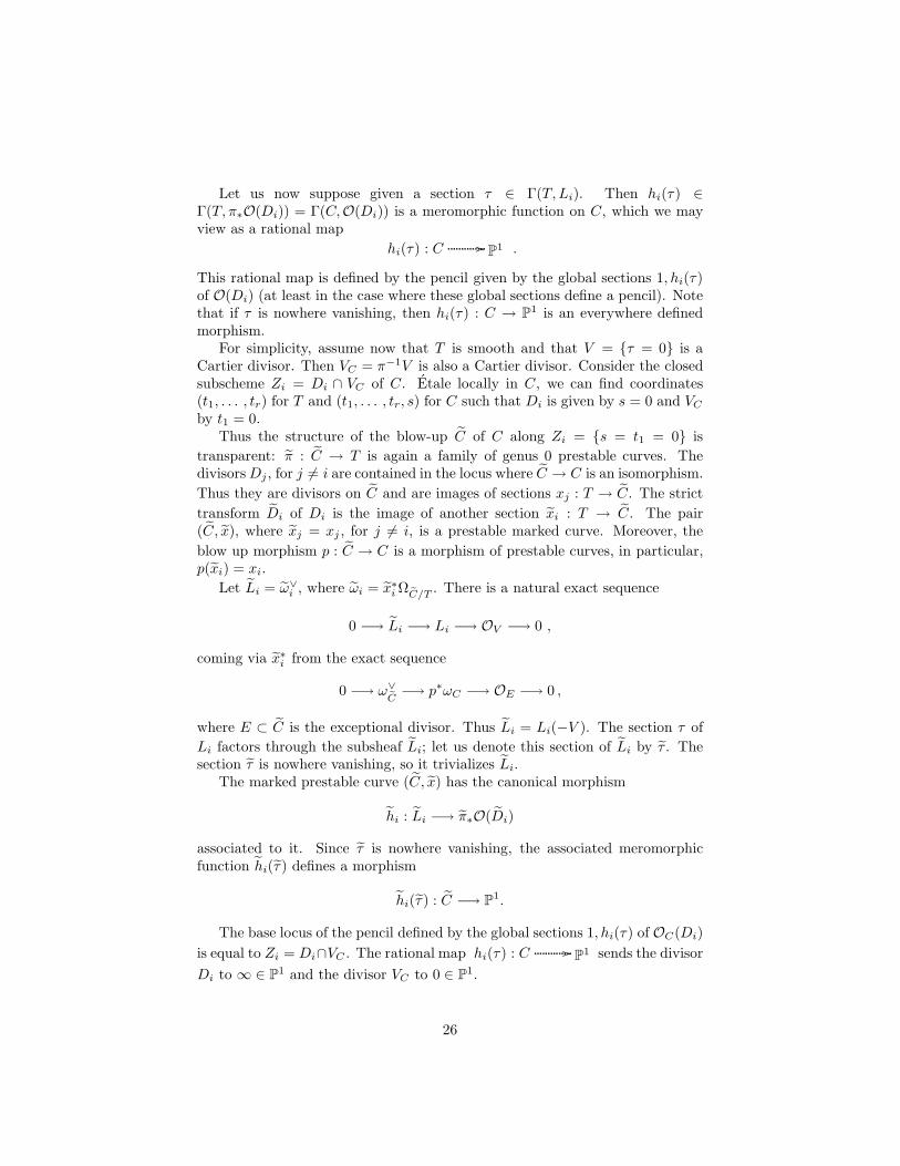
Let us now suppose given a section τ ∈ Γ(T, Li). Then hi(τ) ∈Γ(T, π∗O(Di)) = Γ(C,O(Di)) is a meromorphic function on C, which we mayview as a rational map

hi(τ) : C //P1 .

This rational map is defined by the pencil given by the global sections 1, hi(τ)of O(Di) (at least in the case where these global sections define a pencil). Notethat if τ is nowhere vanishing, then hi(τ) : C → P1 is an everywhere definedmorphism.

For simplicity, assume now that T is smooth and that V = τ = 0 is aCartier divisor. Then VC = π−1V is also a Cartier divisor. Consider the closedsubscheme Zi = Di ∩ VC of C. Etale locally in C, we can find coordinates(t1, . . . , tr) for T and (t1, . . . , tr, s) for C such that Di is given by s = 0 and VCby t1 = 0.

Thus the structure of the blow-up C of C along Zi = s = t1 = 0 is

transparent: π : C → T is again a family of genus 0 prestable curves. ThedivisorsDj , for j 6= i are contained in the locus where C → C is an isomorphism.

Thus they are divisors on C and are images of sections xj : T → C. The strict

transform Di of Di is the image of another section xi : T → C. The pair(C, x), where xj = xj , for j 6= i, is a prestable marked curve. Moreover, the

blow up morphism p : C → C is a morphism of prestable curves, in particular,p(xi) = xi.

Let Li = ω∨i , where ωi = x∗iΩC/T . There is a natural exact sequence

0 −→ Li −→ Li −→ OV −→ 0 ,

coming via x∗i from the exact sequence

0 −→ ω∨

C−→ p∗ωC −→ OE −→ 0 ,

where E ⊂ C is the exceptional divisor. Thus Li = Li(−V ). The section τ of

Li factors through the subsheaf Li; let us denote this section of Li by τ . Thesection τ is nowhere vanishing, so it trivializes Li.

The marked prestable curve (C, x) has the canonical morphism

hi : Li −→ π∗O(Di)

associated to it. Since τ is nowhere vanishing, the associated meromorphicfunction hi(τ ) defines a morphism

hi(τ ) : C −→ P1.

The base locus of the pencil defined by the global sections 1, hi(τ) of OC(Di)

is equal to Zi = Di∩VC . The rational map hi(τ) : C //P1 sends the divisor

Di to ∞ ∈ P1 and the divisor VC to 0 ∈ P1.

26

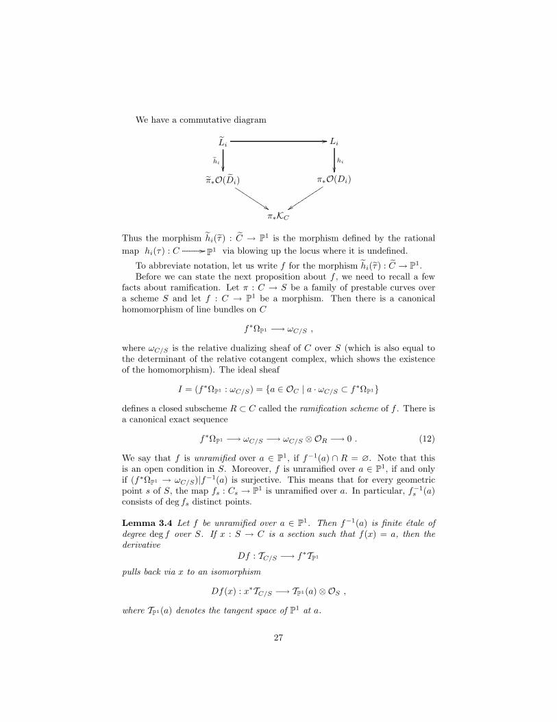
We have a commutative diagram

Li

hi

// Li

hi

π∗O(Di)

$$JJJJJJJJJπ∗O(Di)

zzttttt

ttttt

π∗KC

Thus the morphism hi(τ ) : C → P1 is the morphism defined by the rational

map hi(τ) : C //P1 via blowing up the locus where it is undefined.

To abbreviate notation, let us write f for the morphism hi(τ ) : C → P1.Before we can state the next proposition about f , we need to recall a few

facts about ramification. Let π : C → S be a family of prestable curves overa scheme S and let f : C → P1 be a morphism. Then there is a canonicalhomomorphism of line bundles on C

f∗ΩP1 −→ ωC/S ,

where ωC/S is the relative dualizing sheaf of C over S (which is also equal tothe determinant of the relative cotangent complex, which shows the existenceof the homomorphism). The ideal sheaf

I = (f∗ΩP1 : ωC/S) = a ∈ OC | a · ωC/S ⊂ f∗ΩP1

defines a closed subscheme R ⊂ C called the ramification scheme of f . There isa canonical exact sequence

f∗ΩP1 −→ ωC/S −→ ωC/S ⊗OR −→ 0 . (12)

We say that f is unramified over a ∈ P1, if f−1(a) ∩ R = ∅. Note that thisis an open condition in S. Moreover, f is unramified over a ∈ P1, if and onlyif (f∗ΩP1 → ωC/S)|f−1(a) is surjective. This means that for every geometricpoint s of S, the map fs : Cs → P1 is unramified over a. In particular, f−1

s (a)consists of deg fs distinct points.

Lemma 3.4 Let f be unramified over a ∈ P1. Then f−1(a) is finite etale ofdegree deg f over S. If x : S → C is a section such that f(x) = a, then thederivative

Df : TC/S −→ f∗TP1

pulls back via x to an isomorphism

Df(x) : x∗TC/S −→ TP1(a)⊗OS ,

where TP1(a) denotes the tangent space of P1 at a.

27

Proof. The structure sheaf Of−1(a) of the inverse image f−1(a) fits into theexact sequence

0 −→ OC −→ f∗O(1) −→ Of−1(a) −→ 0 ,

obtained from an identification O(1) = O(a). We get an induced exact sequence

0 −→ OS −→ π∗f∗O(1) −→ π∗Of−1(a) −→ 0 .

Since this sequence stays exact after arbitrary base change, it proves thatπ∗Of−1(a) is locally free of rank deg f (recall that π∗f

∗O(1) is locally free ofrank deg f + 1). By considering the fibers of C → S we see that f−1(a) isquasi-finite over S. Since it is also proper, it is finite, thus flat. Then etale isequivalent to unramified, which can be checked fiber-wise.

Now we come back to f : C → P1 over T , defined above.

Proposition 3.5 The morphism f : C → P1 is a family of degree 1 maps toP1, unramified over ∞ ∈ P1. We have

f−1(∞) = Di ,

and

Df(xi)(τ ) =∂

∂z(∞)⊗ 1 , (13)

where z is the canonical coordinate at ∞ ∈ P1 and ∂∂z (∞) is the evaluation of

∂∂z at z = 0.

Proof. This follows directly from the construction. Formula (13) is a directcalculation.

3.2 A degree d map to P1

Now let us suppose given a regular function b ∈ Γ(T,O) and for every i =1, . . . , d a section τi ∈ Γ(T, Li). Then for each i we have hi(τi) ∈ Γ(C,O(Di))and so for the sum we have

b+

d∑

i=1

hi(τi) ∈ Γ(C,O(

∑iDi)

),

which we may also view as a rational map

b+∑di=1 hi(τi) : C //

P1 . (14)

Note that this is an everywhere defined morphism, if all of the τi are nowherevanishing.

28

Let Vi = τi = 0 and, as above,

Zi = Di ∩ Vi,C .

Let also Z = Z1 ∪ . . . ∪ Zd be the union of these pairwise disjoint closed sub-schemes.

Let us assume, as above, that T is smooth and that the Vi are Cartierdivisors. Let C be the blow-up of C along Z. We get induced sections xi :T → C, making (C, x) a prestable marked curve. We also get induced nowhere

vanishing sections τi ∈ Γ(T, Li) and hence an everywhere defined morphism

f = b+d∑

i=1

hi(τi) : C −→ P1 .

We may also write

f = b+

d∑

i=1

fi , (15)

where fi is the morphism C → P1, defined by hi(τi), as above.Note that the base locus of the pencil defined by the sections 1 and b +∑i hi(τi) of OC(

∑iDi) is Z and so f : C → P1 is the morphism defined by

blowing up the locus of indeterminacy of the rational map (14).

Proposition 3.6 Assume that (C, x) is a stable marked curve. Then (C, f) is

a stable map of degree d. The canonical morphism p : C → C identifies (C, x)

as the stabilization of (C, x). The morphism f : C → P1 is unramified over∞ ∈ P1 and

f−1(∞) =

d∑

i=1

Di . (16)

Assume now that all τi are nowhere vanishing (which implies that C = C)and that all fibers of C are irreducible. Then we have

Df(xi)(τi) =∂

∂z(∞), for all i = 1, . . . , d (17)

and if we let R be the ramification scheme of f , then f |R avoids ∞, thus is aregular function and we have

b =1

2d− 2trR/T (f |R) . (18)

Finally, if g : C → P1 is another family of morphisms of degree d unramified

over ∞ with Properties (16), (17) and (18), then g = f .

29

Proof. The stability condition can be checked on fibers of π. The only po-tentially unstable components in such a fiber (over t) come from an exceptionaldivisor of the blow up. Such a component Ei,t is isomorphic to P1 and intersects

a unique Di at a unique point which gets mapped to ∞. The component Ei,talso intersects Vi,C , the strict transform of Vi,C , in a unique different point,which the map fi sends to 0. Thus fi is of degree 1, when restricted to Ei,t.Since all the other maps fj , for j 6= i, are constant on Ei,t, we see that f |Ei,t is

of degree 1, and hence that Ei,t is a stable component of the map (C, f).

Since p : (C, x) → (C, x) is a morphism of prestable marked curves, and(C, x) is stable, p has to be the stabilization morphism. This follows from theuniversal property of stabilization and the fact that every morphism of stablemarked curves is an isomorphism (see [4], page 27).

By Proposition 3.5 each of the fi is unramified over ∞ and maps Di to ∞.Moreover, τi gets mapped to the canonical tangent vector at ∞ ∈ P1. But fjfor j 6= i is holomorphic (i.e., nowhere equal to ∞) in a neighborhood of Di,

and so adding it to fi does not affect these properties of fi at Di. Hence f isunramified over∞ and f−1(∞) =

∑i Di. Moreover, the derivative of f has the

same behavior at xi as the derivative of fi, and so Formula (17) follows fromProposition 3.5.

Now we assume that all τi are nowhere vanishing. This assumption we makefor C → C to be an isomorphism. We also assume that all the fibers of C areirreducible. This has the nice consequence that, at least locally in T , we canfind an affine coordinate s for C, such that s(xi) has no poles, for any i . Moreprecisely, we can write C as a product T ×P1, such that the sections xi becomefunctions xi : T → P1, and we can arrange things in such a way that xi avoids∞ ∈ P1, for all i. Then we let s be the affine coordinate for P1 −∞. Now thes(xi) are regular functions on T , which we abbreviate by

ai = s(xi) .

We may now use s− ai as equation for Di, so that hi (see (11)) becomes

hi =

1

s− ai+

1

1− d

∑

j 6=i

1

aj − ai

ds(ai) .

We may also use ds(ai) to trivialize ωi and hence Li. We write

τi = qi∂

∂s(ai)

in this trivialization. Thus

hi(τi) = qi

1

s− ai+

1

1− d

∑

j 6=i

1

aj − ai

30

and hence

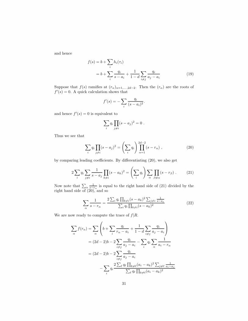
f(s) = b+∑

i

hi(τi)

= b+∑

i

qis− ai

+1

1− d

∑

i6=j

qiaj − ai

(19)

Suppose that f(s) ramifies at (rα)α=1,... ,2d−2. Then the (rα) are the roots off ′(s) = 0. A quick calculation shows that

f ′(s) = −∑

i

qi(s− ai)2

.

and hence f ′(s) = 0 is equivalent to

∑

i

qi∏

j 6=i

(s− aj)2 = 0 .

Thus we see that

∑

i

qi∏

j 6=i

(s− aj)2 =

(∑

i

qi

)2d−2∏

α=1

(s− rα) , (20)

by comparing leading coefficients. By differentiating (20), we also get

2∑

i

qi∑

j 6=i

1

s− aj

∏

k 6=i

(s− ak)2 =

(∑

i

qi

)∑

α

∏

β 6=α

(s− rβ) . (21)

Now note that∑α

1s−rα

is equal to the right hand side of (21) divided by theright hand side of (20), and so

∑

α

1

s− rα=

2∑i qi∏k 6=i(s− ak)2

∑j 6=i

1s−aj∑

i qi∏k 6=i(s− ak)2

(22)

We are now ready to compute the trace of f |R.

∑

α

f(rα) =∑

α

b+

∑

i

qirα − ai

+1

1− d

∑

i6=j

qiaj − ai

= (2d− 2)b− 2∑

i6=j

qiaj − ai

−∑

i

qi∑

α

1

ai − rα

= (2d− 2)b− 2∑

i6=j

qiaj − ai

−∑

i

qi2∑ℓ qℓ∏k 6=ℓ(ai − ak)2

∑j 6=ℓ

1ai−aj∑

ℓ qℓ∏k 6=ℓ(ai − ak)2

31

(by Equation (22))

= (2d− 2)b− 2∑

i6=j

qiaj − ai

−∑

i

qi2qi∏k 6=i(ai − ak)2

∑j 6=i

1ai−aj

qi∏k 6=i(ai − ak)2

(because for ℓ 6= i the product vanishes)

= (2d− 2)b− 2∑

i6=j

qiaj − ai

− 2∑

i

qi∑

j 6=i

1

ai − aj

= (2d− 2)b .

It remains to prove the uniqueness claim. But it is easy to see that

f(s) = c+

d∑

i=1

qis− ai

is the most general degree d morphism which maps ai to∞, for all i, and satisfies

d

ds

1

f(s)

∣∣∣∣s=ai

=1

qi,

for all i. Thus the uniqueness follows.

3.3 The universal situation

Consider M0,d, the scheme of stable curves of genus zero marked by d =1, . . . , d. Let π : C →M0,d be the universal curve and x1, . . . , xd the univer-sal sections. Let ωi and Li be line bundles over M0,d defined as above. Finally,define

T = A1 ×

d∏

i=1

Li ,

where the product is taken over M0,n. Thus T is a vector bundle of rank d+ 1overM0,d. In particular, T is a smooth scheme of dimension d−3+d+1 = 2d−2.When we pull back any of the M0,d-schemes Li or C to T , we endow them witha subscript T (which we also occasionally omit).

If S is a scheme, then we may think of S-valued points of T as 2d+ 2-tuples

(C, x, b, τ) = (C, x1, . . . , xd, b, τ1, . . . , τd) ,

where (C, x) ∈ M0,d(S) is a stable marked curve over S, b ∈ A1S is a regular

function on S and τi is a tangent vector of C at xi, or rather a section of Liover S. Similarly, S-valued points of CT are 2d+ 3-tuples

(C, x, b, τ,∆),

32

where (C, x, b, τ) is as above and ∆ ∈ C(S).

The various projections of A1×∏di=1 Li onto its components define a canon-

ical regular function b ∈ Γ(T,O) and canonical sections τi ∈ Γ(T, Li,T ). Theseare, of course, the universal b, τ . As in Section 3.2, we let Z = Z1∪. . .∪Zd ⊂ CT ,where Zi = Di ∩ τi = 0, and we blow up CT at Z to obtain π : C → T .

As in Section 3.1, we get for every i a meromorphic function fi = hi(τi) ∈

Γ(CT ,O(Di)

), which we can identify with the meromorphic function hi(τi) ∈

Γ(C,O(Di)

). Note that fi is an everywhere non-vanishing section of the line

bundle O(Di). We also get for every i 6= j a regular function

ηij = fi(xj) = hi(xj)(τi) = hi(τi)(xj) . (23)

The ηij will be very useful in Section 4.As in Section 3.2, we get a meromorphic function

b+

d∑

i=1

hi(τi) ∈ Γ(CT ,O(

∑iDi)

),

and an induced morphismf : C −→ P

1 .

By Proposition 3.6 (C, f) is a stable map of degree d over T , and so we get aninduced morphism

T −→M0,0(P1, d) . (24)

The symmetric group Sd acts on M0,d from the right by

(C, x1, . . . , xd) · σ = (C, xσ(1), . . . , xσ(d)) .

We have compatible actions on T given by

(C, x1, . . . , xd, b, τ1, . . . , τd) · σ = (C, xσ(1), . . . , xσ(d), b, τσ(1), . . . , τσ(d))

and on CT given by

(C, x1, . . . , xd, b, τ1, . . . , τd,∆) · σ = (C, xσ(1), . . . , xσ(d), b, τσ(1), . . . , τσ(d),∆) .

The vector bundle∏di=1 Li overM0,d descends to a vector bundle E = [

∏Li/Sd]

of rank d over [M0,d/Sd], which does not split anymore. But still, [T/Sd] →[M0,d/Sd] is a vector bundle of rank d+ 1.

For all σ ∈ Sd, the induced automorphism of CT identifies Zi with Zσ(i)

and so Z ⊂ CT is an invariant subscheme under the Sd-action. Thus we getan induced action of Sd on the blow-up C. This action is compatible with theprojection π : C → T and so we get an induced prestable curve [C/Sd]→ [T/Sd].

Note also that f : C → P1 is Sd-invariant. This follows from Formula (15) andthe fact that the action of σ exchanges fi and fσ(i). Thus we get an induced

morphism [f/Sd] : [C/Sd]→ P1, and so we see that (24) induces a morphism

[T/Sd] −→M0,0(P1, d) . (25)

33

Theorem 3.7 The morphism (25) is an isomorphism onto the open substackof M0,0(P1, d) consisting of stable maps which are unramified over ∞ ∈ P1.

Before proving the theorem, we prepare a little more. We already remarkedthat ‘unramified over ∞’ is an open condition on stable maps to P1. So thestable maps unramified over ∞ form an open substack U ⊂ M0,0(P1, d). Let zbe the canonical coordinate at ∞ on P

1. If (C, f) ∈ M0,0(P1, d)(S) is a stablemap parametrized by the scheme S, then f∗(z) defines the closed subschemef−1(∞) of C.

Assume that the stable map (C, f) is unramified over∞. Then f−1(∞)→ Sis finite etale of degree d. We call an isomorphism

φ : d× S −→ f−1(∞)

an indexing of f−1(∞). The local indexings form an S-scheme

P = IsomS(d× S, f−1(∞)) ,

which is a principal (right) Sd-bundle over S. In particular, P → S is finiteetale of degree d!.

Let U ′ be the stack of triples (C, f, φ), where (C, f) ∈M0,0(P1, d) is a stablemap unramified over ∞ and φ is an indexing of f−1(∞). Thus U ′ → U is aprincipal Sd-bundle, in fact, U ′ → U is the stack of indexings of the universalf−1(∞). It is not difficult to see that U ′ is a scheme.

Now consider the stable map (C, f) defined over T . By Proposition 3.6 wehave that

f−1(∞) =

d∑

i=1

Di .

Thus (C, f) comes with a canonical indexing of f−1(∞). Therefore, we get amorphism T → U ′. In other words, the morphism (24) lifts in a natural way toU ′ →M0,0(P1, d).

Theorem 3.7 now follows from the following proposition.

Proposition 3.8 The canonical morphism T → U ′ is an isomorphism ofschemes with Sd-action.

Proof. Let us define the inverse of T → U ′. Let (C, f, φ) be an S-valuedpoint of U ′. We need to associate to (C, f, φ) an S-valued point of T . Since U ′

is smooth, we may assume that S is smooth and that the structure morphismS → U ′ is etale.

Let S′ ⊂ S be the locus over which f does not contract any components ofC. Since a contracted component has at least 3 special points, the complementof S′ in S has codimension at least 3. Thus to define a regular function on S isequivalent to defining a regular function on S′ (codimension 2 would suffice forthis). Let C′ → S′ be the restriction of C → S to S′.

34

Let R be the ramification scheme of f . Over S′ the exact sequence (12) isexact on the left also

0 −→ f∗ΩP1 −→ ωC′/S′ −→ ωC′/S′ ⊗OR′ −→ 0

and commutes with base change to the fibers of C′ → S′. Hence we see thatover S′ the pullback R′ = S′ ×S R is finite and flat of degree 2d− 2 over S′.

By assumption, R′∩f−1(∞) = ∅ and so f |R′ factors through A1 = P1−∞,i.e., f |R′ is a regular function on R′. Then we can take the trace to get a regularfunction

trR′/S′(f |R′)

on S′, which extends uniquely to a regular function on S, which we denote bytrR/S(f |R), by abuse of notation. Define

b =1

2d− 2trR/S(f |R) .

Thus b is the average of the ramification points of the stable map f .The isomorphism φ : d×S → f−1(∞) defines d sections x1, . . . , xd : S → C.

Consider the derivativeDf : TC/S −→ f∗TP1

and pull it back via xi to get an isomorphism

Df(xi) : Li = x∗i TC/X −→ x∗i f∗TP1 = TP1(∞)⊗OS ,

where TP1(∞) is the tangent space of P1 at ∞ (see Lemma 3.4). Taking thepreimage of ∂

∂z (∞)⊗ 1 under Df(xi) yields a section τi ∈ Γ(S,Li).Stabilizing (C, x) defines a stable marked curve

(C, x) = (C, x)stab .

The stabilization morphism p : C → C induces a homomorphism

Li → Li = x∗i TC/S ,

which maps τi to a section τ i ∈ Γ(S,Li).Now we have defined an S-valued point

(C, x1, . . . , xd, b, τ1, . . . , τd)

of T , which we declare to by the image of (C, f, φ), thus defining a morphismU ′ → T .

Claim I. The composition T → U ′ → T is equal to the identity.To prove this claim, we start with an S-valued point (C, x, b, τ) of T . We

pass to (C, x, f), which defines a point of U ′. From Proposition 3.6 it follows

that (C, x) is the stabilization of (C, x), and so the marked curve associated to

(C, x, f) under U ′ → T is (C, x). It remains to prove that b = 12d−2 tr(f |R) and

35

τi = Df(xi)−1( ∂∂z (∞)). But these facts may be checked on a dense open subset

of S (or T ), and so they follow from Proposition 3.6, Equations (17) and (18).Claim II. The composition U ′ → T → U ′ is the identity.To prove this claim, we may pass to a dense open substack of U ′, because

the target U ′ is separated. We start with an S-valued point (C, f, φ) of U ′,which defines a prestable marked curve (C, x). If we assume that S is etale overU ′, then the locus S′ ⊂ S over which (C, x) is stable is dense in S. Over S′,neither stabilization nor blowing up changes (C, x) at all, so that, at least overS′, the curve (C, x) agrees with the one obtained by applying the compositionU ′ → T → U ′. To check that also the map f does not change after passingthrough U ′ → T → U ′, we may make S′ still smaller, and apply the uniquenesspart of Proposition 3.6.

Remark Denote by Ua the open substack of M0,0(P1, d) consisting of mapswhich are unramified over a ∈ P1. Obviously, Ua is isomorphic to U∞ andhence Ua ∼= T , for all a. Choosing any N distinct points a1, . . . , aN ∈ P1, whereN > 2d−2, let Ui = Uai

. Then U1, . . . , UN coverM0,0(P1, d). Thus it is possibleto obtain M0,0(P1, d) by gluing together N copies of [T/Sd]. Ultimately, thisleads to a complete description of the stable map stack M0,0(P1, d) in terms ofthe stable curve space M0,d.

In this way, many questions about M0,0(P1, d) can be reduced to questionsabout M0,d.

The action of the multiplicative group

We endow P1 with the right action of the group G (see Remark 1.2) given inExample 1.3. As usual, we get an induced (right) action of B on M0,0(P1, d)given by

(C, f)(a, λ) =(C, (a, λ) f

).

As in Remark 1.2, this means that we have a Gm-action and an equivariantvector field on M0,0(P1, d).

Since ∞ ∈ P1 is a fixed point for the Gm-action on P1, it is obvious thatthe stack of stable maps unramified over ∞ is invariant under the Gm-actionon M0,0(P1, d). In this section we will determine the induced Gm-action on T .Since the stack of maps unramified over ∞ is not invariant under all of B, wecannot describe an induced action of B on T , but, of course, we can pull backthe equivariant vector field to T . Since this is more involved, we shall postponeit to Section 4.

Proposition 3.9 Let Gm act on T through scalar multiplication on the vectorbundle T over M0,d. This Gm-action commutes with the Sd-action, hence in-duces a Gm-action on [T/Sd]. Then the open immersion (25) of Theorem 3.7 isGm-equivariant.

36

Proof. Let t ∈ T . We have to show that for λ ∈ C∗ we have

(Ct, λ ft) ∼= (Cλt, fλt)

as stable maps. But to check that two automorphisms of T agree, we may passto a dense open subscheme of T . So we may assume that Ct = Cλt = P

1 andthat ft : P1 → P1 is given by (19). Then the linearity of (19) in (b, q1, . . . , qd),which are coordinates on the fibers of T →M0,d, implies that λft = fλt, whichimplies the claim.

3.4 Maps to Pn

Let Y ⊂ Pn be the open subvariety defined by

Y = 〈x0, . . . , xn〉 ∈ Pn | x0 6= 0 or x1 6= 0 .

The map 〈x0, . . . , xn〉 7→ 〈x0, x1〉 defines a morphism p : Y → P1.

Y

p

// Pn

P1

Let us denote the fiber of p over∞ by Y∞. Thus Y∞ = 〈0, 1, y2, . . . , yn〉 ∈ Pn,and Y∞ is canonically identified with An−1.

We will describe the open substack U ⊂ M0,0(Pn, d) consisting of stablemaps (C, f) such that f(C) ⊂ Y and (C, pf) is unramified over∞ = 〈0, 1〉 ∈ P1.In fact, we will show that U is a vector bundle over M0,d modulo the action ofSd.

Let U1 ⊂M0,0(P1, d) be the open substack of stable maps unramified over∞.By definition, we have a cartesian diagram

U

// M0,0(Y, d)

//

M0,0(Pn, d)

U1

// M0,0(P1, d)

Let

T = A1 ×

(d∏

i=1

Li

)×(A

1 × Ad)n−1

, (26)

where the product is taken over M0,d. We will write an element of T (S), for ascheme S, as

(C, x, b, τ, r)

where (C, x) = (C, x1, . . . , xd) ∈ M0,d(S) is a stable marked curve over S,b = (b1, . . . , bn) is an n-tuple of regular functions on S, τ = (τ1, . . . , τd), where

37

τi is a section of Li over S and r = (rν,i) ν=2,... ,n

i=1,... ,dis a d(n − 1)-tuple of regular

functions on S. The order of the various coordinates in (26) is(b1, (τi), b2, (r2,i), . . . , bn, (rn,i)

).

The reason for this order will become clear below.For notational convenience, we assign the value 1 to r1,i, for all i = 1, . . . , d.For ν = 1, . . . , n consider

bν +

d∑

i=1

hi(rν,iτi) ∈ Γ(CT ,O(

∑iDi)

).

Let, as above, Z = Z1 ∪ . . . ∪ Zd, where Zi = Di ∩ τi = 0. After blowing upZ ⊂ CT we get a morphism

f = 〈1, ϕ1, . . . , ϕn〉 : C −→ Y ,

where

ϕν = bν +

d∑

i=1

hi(rν,i τi) = bν +

d∑

i=1

rν,ifi . (27)

This follows easily from the fact that already the sections 1 and ϕ1 = b1 +∑i hi(τi) = b1 +

∑i fi of O(

∑i Di) generate this invertible sheaf, so that any

values for ϕ2, . . . , ϕn define a morphism to Pn. But, for the same reason, thismorphism factors through Y .

Thus (C, f) is a stable map of degree d parametrized by T and hence we geta morphism

T −→ U ⊂M0,0(Pn, d) . (28)

We will show that (28) induces an isomorphism [T/Sd] ∼= U .Let us write ri = 〈0, 1, r2i, . . . , rni〉. Then we can say that r1, . . . , rd ∈ Y∞

are the points where our stable map intersects Y∞ and τi gives the ‘speed’ withwhich the map passes through the point ri. The coordinate bν gives the averageof the ramification points of the projection onto the ν-th coordinate axis.

The next proposition makes this more precise.

Proposition 3.10 For any i = 1, . . . , d the composition f xi defines a mor-phism

f xi : T −→ Y∞ ,

which is given by f xi = ri.Fix a value of ν = 2, . . . , n. Over the locus where (rν,1, . . . , rν,d) 6= 0 we can

compose f with the projection pν onto the coordinate axis 〈y0, 0, . . . , yν , . . . , 0〉to obtain a stable map fν = pν f unramified over ∞ = 〈0, . . . , 1, . . . , 0〉. Let

Rν ⊂ C be the ramification scheme of fν . Then we have

bν =1

2d− 2trRν/T (f |Rν) .

38

Proof. To check that the two morphism f xi and ri agree, we may restrictto the locus where none of the τi or rν,i vanish. Then we need to prove that

(ϕ2(s)

ϕ1(s), . . . ,

ϕn(s)

ϕ1(s)

)∣∣∣∣s=xi

= (r2,i, . . . , rn,i) .

This follows from (17), using l’Hopital’s rule. The second claim, giving themeaning of the bν , follows directly from (18).

Let T1 → M0,0(P1, d) be the scheme constructed in Section 3.3 and calledsimply T there. By forgetting the new coordinates we introduced here, we geta morphism T → T1, which makes T into a vector bundle over T1. Note that

T

// M0,0(Y, d)

T1

// M0,0(P1, d)

commutes. So letting U be the fibered product U = T1×U1U we get the diagram

T //

==

==

==

== U

// U

//

M0,0(Y, d)

// M0,0(Pn, d)

T1// U1

// M0,0(P1, d)

By Proposition 2.1 the scheme U is also a vector bundle over T1.

Proposition 3.11 The morphism T → U is an isomorphism of vector bundlesover T1. Hence, [T/Sd] ∼= U .

Proof. To check that T → U is a morphism of vector bundles is made easierby the fact that it suffices for this to prove compatibility with the (linear) Gm-actions. This is proved directly from the definitions of the two vector bundlestructures using Proposition 3.10.

Since both vector bundles have the same rank (d + 1)(n − 1), for the iso-morphism property it suffices to prove strict injectivity, i.e., injectivity overevery base change to a point of T1. Then the claim also follows easily fromProposition 3.10.

Proposition 3.12 Let Gm act on T by(C, x, b1, (τi), b2, (r2,i), . . . , bn, (rn,i)

)λ

=(C, x, b1λ, (τiλ), b2λ

2, (r2,iλ), . . . , bnλn, (rn,iλ

n−1)).

In other words, we let bν have weight ν, we let τi have weight 1 and we let rν,ihave weight ν − 1. Then T →M0,0(Pn, d) is Gm-equivariant.

Proof. This also follows from Proposition 3.10 using the definition of theGm-action on Pn from Example 1.3.

39

3.5 The degree 2 case

Since M0,2 does not exist, the above considerations to not apply directly to thedegree 2 case. We show how to treat this case here.

Let U ⊂ M0,0(Pn, 2) be, as above, the open substack of stable maps (C, f)such that

(i) f(C) ⊂ Y ,(ii) p f is unramified over ∞ ∈ P1 (or f intersects Y∞ transversally).

We will show how to write U as the stack quotient [A3n−1/S2], for a suitableS2-action on A3n−1.

Let T1 = A2, with coordinates b, q. Let C = T1×P1, with sections x1 : T1 →T1×P1; t 7→ (t, 0) and x2 : T1 → T1×P1; t 7→ (t,∞). Let s be the canonical affinecoordinate on P

1, z = 1s . Apply the program of Section 3.2 with b, τ1 = ∂

∂s(0)

and τ2 = q ∂∂z (∞) to obtain a stable map of degree 2 from C to P1, unramified

over ∞, where C is the blow up of C = T1 × P1 at Z = Z2 = D2 ∩ q = 0.

Note that even though (C, x1, x2) is not a stable curve, (C, x1, x2, f) is a stablemap. Over T1 − Z, the morphism f is given by

f(s) = b+1

s+ qs .

Let S2 act trivially on T1, and on T1 × P1 via the involution

σ : T1 × P1 −→ T1 × P

1

(b, q, s) 7−→ (b, q,1

qs) .

Note that σ extends uniquely to an automorphism σ of C, giving rise to anaction of S2 on C. Note also that f σ = f , and so we get a stable map

[C/S2]

f //P1

[T1/S2]

of degree 2. Thus we have a morphism [T1/S2]→M0,0(P1, 2).

Lemma 3.13 This morphism [T1/S2] → M0,0(P1, 2) is an isomorphism ontothe open substack U .

Now letT = T1 × (A1 × A

2)n−1 ,

with additional coordinates (b2, r21, r22), . . . , (bn, rn1, rn2). Let CT = C ×T1T

and define ϕ : CT → Pn by ϕ = 〈1, f, ϕ2, . . . , ϕn〉, where

φν(s) = bν + rν11

s+ rν2 qs ,

40

for ν = 2, . . . , n.Let S2 act on T by fixing T1 and all bν , and exchanging rν1 with rν2, for

ν = 2, . . . , n. Finally, let S2 act on CT diagonally, and denote the correspondinginvolution of CT by σT . Then ϕ σT = ϕ and so we get an induced stable mapϕ : [CT /S2] → P

n parametrized by [T/S2] and hence a morphism [T/S2] →M0,0(Pn, 2).

Theorem 3.14 The morphism [T/S2] → M0,0(Pn, 2) is an isomorphism ontothe open substack U . Moreover,

[T/S2]

// M0,0(Y, 2)

[T1/S2] // M0,0(P1, 2)

(29)

is a pullback diagram of vector bundles.

Moreover, (29) is Gm-equivariant if we let Gm act on T by

(b, q, . . . , (bν , rν1, rν2), . . .

)· λ =

(bλ, qλ2, . . . , (bνλ

ν , rν1λν−1, rν2λ

ν−1), . . .).

4 The vector field

4.1 Some deformation theory

Recall that the group G = Ga ⋊Gm acts on Pn, as described in Example 1.3. Weget induced actions on the stable map stacks M0,0(Pn, d) and M0,1(Pn, d) bythe usual formula (C, x, f) · g = (C, x, g f). The latter stack we may interpretas the universal curve C over M0,0(Pn, d), and so we have a diagram

C

π

f // Pn

M0,0(Pn, d)

of stacks with G-equivariant morphisms. If we differentiate the Ga-actions, weobtain Gm-equivariant vector fields W on Pn, V on M0,0, (P

n, d) and U on C. Ofcourse, U maps to V and W under Dπ and Df , respectively. We are concernedwith finding V .

In this section we will show that V and U are determined uniquely, simplyby the fact that Dπ(U) = V and Df(U) = W . The same is then true for theetale M0,0(Pn, d)-scheme T : we know that we have found V |T if we can find a

vector field U on C that simultaneously lifts V |T and W .

41

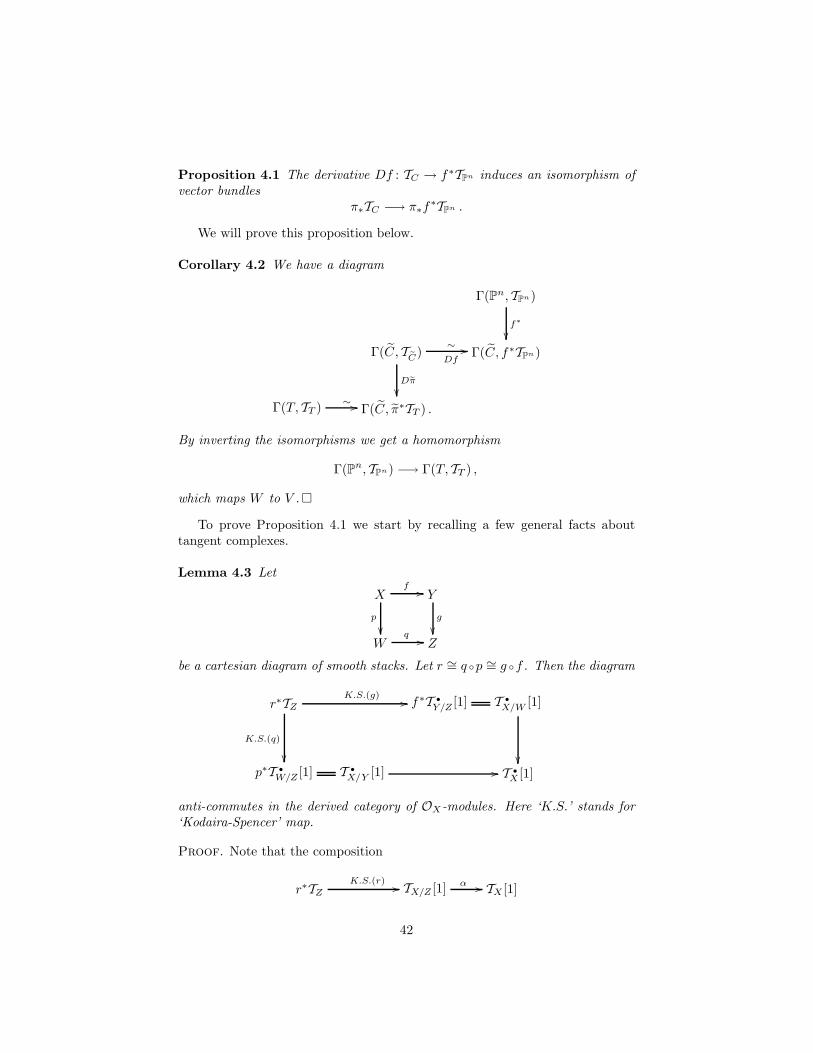
Proposition 4.1 The derivative Df : TC → f∗TPn induces an isomorphism ofvector bundles

π∗TC −→ π∗f∗TPn .

We will prove this proposition below.

Corollary 4.2 We have a diagram

Γ(Pn, TPn)

f∗

Γ(C, TC)

∼

Df//

Dπ

Γ(C, f∗TPn)

Γ(T, TT )∼ // Γ(C, π∗TT ) .

By inverting the isomorphisms we get a homomorphism

Γ(Pn, TPn) −→ Γ(T, TT ) ,

which maps W to V .

To prove Proposition 4.1 we start by recalling a few general facts abouttangent complexes.

Lemma 4.3 Let

X

p

f // Y

g

W

q // Z

be a cartesian diagram of smooth stacks. Let r ∼= q p ∼= g f . Then the diagram

r∗TZK.S.(g) //

K.S.(q)

f∗T •

Y/Z [1] T •

X/W [1]

p∗T •

W/Z [1] T •

X/Y [1] // T •

X [1]

anti-commutes in the derived category of OX-modules. Here ‘K.S.’ stands for‘Kodaira-Spencer’ map.

Proof. Note that the composition

r∗TZK.S.(r) // TX/Z [1]

α // TX [1]

42

is zero. On the other hand, we have

TX/Z [1] = TX/Y [1]⊕ TX/W [1]

and under this decomposition we have K.S.(r) = K.S.(q) ⊕K.S.(g). Applyingα, we get

0 = α K.S.(r) = α K.S.(q) + α K.S.(g) .

This is what we wanted to prove.

Lemma 4.4 Again, considering a cartesian diagram as in the previous lemma,there is a canonical homomorphism of distinguished triangles

f∗T •

Y/Z//

f∗T •

Y// f∗g∗T •

Z

K.S.(g)//

K.S.(q)

f∗T •

Y/Z [1]

T •

X

β // f∗T •

Y// T •

X/Y [1]−β[1] // T •

X [1] .

The upper triangle is the pullback under f of the distinguished triangle associatedwith g, the lower triangle is a shift of the distinguished triangle associated withf .

Proof. We have to show that the three squares commute. The last one isLemma 4.3.

In any cartesian diagram as the one under consideration, there is a homo-morphism from the distinguished triangle for p to the pullback under f of thedistinguished triangle for g. Similarly, for f and q. Picking out appropriate com-mutative squares from these homomorphisms of distinguished triangles provesthe commutativity of the other two squares.

Consider the morphism of stacks

h : M0,0(Pn, d) −→M0,0 .

Here M0,0 is the Artin stack of prestable curves of genus zero. The morphism his given by forgetting the map, retaining only the prestable curve (and not sta-bilizing). The fiber of h over a prestable curve C is equal to an open subschemeof Mor(C,Pn), the scheme of morphisms from C to Pn.

Deformation theory for morphisms shows that Mor(C,Pn) is smooth withtangent space H0(C, f∗TPn) at the point f : C → Pn of Mor(C,Pn). It followsthat h is smooth with relative tangent bundle

TM/M = π∗f∗TPn .

We shall now apply Lemma 4.4 to the cartesian square

C

π // M0,0(Pn, d)

h

C

π // M0,0

43

where C→M0,0 is the universal curve over M0,0. We obtain the homomorphismof distinguished triangles

π∗TM/M//

π∗TM //

π∗h∗T •

M//

π∗TM/M[1]

TC // π∗TM // T •

C/M[1] // TC [1]

and by adjointness, the homomorphism

TM/M//

φ

TM //

φ′

h∗T •

M//

φ′′

TM/M[1]

Rπ∗TC // Rπ∗π∗TM // Rπ∗T •

C/M[1] // Rπ∗TC [1] .

By the projection formula we have Rπ∗π∗TM = TM ⊗Rπ∗OC = TM . Therefore

φ′ is an isomorphism. We also have that Rπ∗T•

C/M[1] = h∗Rπ∗T

•

C/M[1]. Thus φ′′

may be viewed as the pullback under h of the Kodaira-Spencer homomorphismT •

M→ Rπ∗T

•

C/M[1], which is an isomorphism by the deformation theory ofprestable curves.

Since both φ′ and φ′′ are isomorphisms, so is φ : TM/M → Rπ∗TC .Finally, let us consider the composition of homomorphisms of vector bundles

on C

π∗TM/M = TC/C −→ TCDf−→ f∗TPn .

Again, by adjointness, we get an induced homomorphism in the derived categoryof M0,0(Pn, d)

TM/M

φ−→ Rπ∗TC

ψ−→ Rπ∗f

∗TPn .

We just saw that φ is an isomorphism, and the composition ψ φ is an isomor-phism by the deformation theory of morphisms. Therefore, ψ is an isomorphism.Since Rπ∗f

∗TPn = π∗f∗TPn , we deduce that Rπ∗TC = π∗TC , and that we have

an isomorphism of vector bundles

π∗TC −→ π∗f∗TPn

which is induced by the derivative Df : TC → f∗TPn . This finishes the proof ofProposition 4.1.

4.2 The degree 3 case

We will now use Corollary 4.2 to determine the vector field V on T in the caseof d = 3.

So let d = 3. Then M0,3 = Spec C. The universal curve C over M0,3 isisomorphic to P1, with 3 marked points x1, x2, x3 ∈ P1. The vector bundle Tover M0,3 = Spec C is just a vector space. We have canonically

T =(C⊕ L1 ⊕ L2 ⊕ L3

)⊕(C⊕ C

3)(n−1)

,

44

where Li = TP1(xi) is the tangent space of P1 at a marked point.Every vector space E has a canonical vector field on it, namely the vector

field that takes the value e ∈ E at the point e ∈ E. This makes sense, becauseevery tangent space of E is canonically identified with E. If we choose a basis(ei) for E, then this vector field is given by

∑i xi

∂∂xi

=∑

i xiei, where (xi) arethe coordinates on E induced by the basis (ei). We denote the canonical vectorfield on Li by τi, for i = 1, 2, 3. Because of the product decomposition of T , wecan also think of the τi as canonical vector fields on T .

Recall that the first coordinate of every quadruple of coordinates on T iscalled bν , where ν = 1, . . . , n. The latter three coordinates in the latter n − 1quadruples of coordinates are called (rν,i)ν=2,... ,n, i=1,2,3. Recall also that wewrite r1,i = 1, i = 1, 2, 3, for notational convenience. For further notationalconvenience we write rν,0 = bν , for ν = 1, . . . , n. This then defines rν,i forall ν = 1, . . . , n and all i = 0, 1, 2, 3. For every ν = 1, . . . , n we combinerν,0 . . . , rν,3 into the column vector rν . Thus

r1 =

b1111

and rν =

bνrν,1rν,2rν,3

for ν = 2, . . . , n

Because of the product decomposition of T , every vector field on T is in acanonical way a sum of 4n components. All but three are canonically identifiedwith regular functions on T . We combine groups of four components into oneas follows.

V1 = V1,0∂

∂b1+

3∑

i=1

V1,i ,

and for ν = 2, . . . , n

Vν = Vν,0∂

∂bν+

3∑

i=1

Vν,i∂

∂rν,i.

It will be convenient to introduce the following abbreviations:

η(2)i = −

∏

j 6=i

ηij

and for all µ ≥ 1

θ(µ)i =

∑

j 6=i

ηµ−1ij ηji ,

(so that the upper indices denote the degree). Here the ηij are the canonicalregular functions on T introduced in (23). Finally, let

ℓi = r2,i − 2b1 − 4θ(1)i ,

for i = 1, 2, 3.

45

Proposition 4.5 With this notation, the vector field V on T is given by

V1 = r2 − Er1 +

0ℓ1τ1ℓ2τ2ℓ3τ3

=

b2 − b21 +

∑i η

(2)i + 5

∑i θ

(2)i

ℓ1τ1ℓ2τ2ℓ3τ3

,

Vν = rν+1 − Erν , for ν = 2, . . . , n− 1 ,

Vn = −Ern .

Here E is the 4× 4 matrix

E =

b1 η(2)1 + 5θ

(2)1 η

(2)2 + 5θ

(2)2 η

(2)3 + 5θ

(2)3

1 ℓi + b1 + 3θ(1)1 η21 η31

1 η12 ℓ2 + b1 + 3θ(1)2 η32

1 η13 η23 ℓ3 + b1 + 3θ(1)3

.

In the case n = 1, the formula for V1 is used, not the formula for Vn. Moreover,b2 and r2,i are set equal to 0 in this case.

Proof. It suffices to check these formulas on a dense open subset of T . So weshall restrict to the subscheme of T where none of the τi vanish, so that we mayassume that C = CT = T × P1. Then all we have to do is exhibit a verticalvector field U for the projection T × P1 → T such that Df(V +U) = W . Then

the vector field U on C is given by U = V +U , over this open subscheme of C.The relative vector field U is very easy to describe. For every point t of T ,

we have given 3 tangent vectors on P1, namely the τi(t) ∈ TP1(xi). On P1 thereis a unique vector field U(t) taking this prescribed value τi(t) at the point xi,for i = 1, 2, 3. This defines U .

The details follow below.

Lemma 4.6 Let T be a scheme and τi ∈ Γ(T, Li), for i = 1, 2, 3 a section ofLi over T . Then the formula

U =

3∑

i=1

∏

j 6=i

(1−

sisi(xj)

) τidsi(xi)

∂

∂si,

defines a relative vector field U ∈ Γ(T×P1, TT×P1/T ) = Γ(T×P1, TP1), which has

the property that U(xi) = τi, for i = 1, 2, 3. Here si is a degree one meromorphicfunction on P1, which vanishes at xi (i.e., a parameter at xi).

Let fi = hi(τi), for i = 1, 2, 3 be the meromorphic function on T × P1

considered above (see Corollary 3.2). Then we have

U(fi) = 2θ(2)i + η

(2)i + 2θ

(1)i fi − f

2i ,

for every i = 1, 2, 3.

46

Proof. It is not difficult to see that the formula for U defines a vector fieldon P1, no matter the choice of the si, even if si(xj) = ∞, for some j 6= i. Theverification that U(xi) = τi is then easy.

The calculation of U(fi) is somewhat tedious. It can be done by choosing acoordinate s for P

1, which does not take the value ∞ at any of the xi. Thenwrite ai = s(xi) and si = s − ai. Finally, write qi = τidsi(xi). With thesechoices we have

U =3∑

i=1

qi

∏

j 6=i

s− ajai − aj

∂

∂s

and

fi = qi

1

s− ai−

1

2

∑

j 6=i

1

aj − ai

.

Thus

U(fi) = −

3∑

k=1

qk

∏

j 6=k

s− ajak − aj

qi

(s− ai)2

and this can be compared to the given formula for U(fi).

Lemma 4.7 With the same notation, we have for i 6= j

fifj = ηjifi + ηijfj + 3ηijηji .

In particular, summing over all i and j such that i 6= j,

∑

i6=j

fifj = 2∑

i6=j

ηjifi + 3∑

i6=j

ηijηji .

Proof. This can be proved similarly.

In view of the formula for W given in Example 1.3, the following corollarynow finishes the proof of Proposition 4.5.

Corollary 4.8 If we were to define a vector field V on T by the formulas ofProposition 4.5, then we would have

V (ϕν) + U(ϕν) = ϕν+1 − ϕ1ϕν ,

for ν < n and

V (ϕn) + U(ϕn) = −ϕ1ϕn .

Here the ϕν are the components of the morphism f : C → Pn given as in (27)

by ϕν = bν +∑3i=1 rν,ifi.

47

Proof. We note that τj(fi) = δijfi (Kronecker delta). Moreover, V (fi) = ℓifi.Therefore, we need to prove the following formulas. First

V1,0 +∑

i

ℓifi +∑

i

U(fi) = b2 +∑

i

r2,ifi −(b1 +

∑

i

fi)2,

then for every 1 < ν < n

Vν,0 +∑

i

rν,iℓifi +∑

i

Vν,ifi +∑

i

rν,iU(fi)

= bν+1 +∑

i

rν+1,ifi −(b1 +

∑

i

fi)(bν +

∑

i

rν,ifi),

and finally,

Vn,0 +∑

i

rn,iℓifi +∑

i

Vn,ifi +∑

i

rn,iU(fi)

= −(b1 +

∑

i

fi)(bn +

∑

i

rn,ifi).

All of these formulas follow easily from Lemmas 4.6 and 4.7.

To make the relationship between vector fields and regular functions on theLi explicit, we identify the universal curve C with P1, with affine coordinates. Then we choose for x1, x2 and x3, the points 0, 1 and ∞. We choose localparameters 1

2s at 0, s−12s at 1 and 1

2−2s at ∞. This trivializes L1, L2 and L3,and we write, as usual, the induced coordinates on Li as qi. With this notationthe universal map is given by

ϕν(s) = bν + rν,1 q12− s

s+ rν,2 q2

s+ 1

s− 1+ rν,3 q3(1− 2s) ,

for all ν = 1, . . . , n. Moreover, we have τi = qi and

η12 = q1 η13 = −q1

η21 = −q2 η23 = q2

η31 = q3 η32 = −q3 .

The matrix E then takes the following shape:

E =

b q1(q1 − 5(q2 + q3)

)q2(q2 − 5(q1 + q3)

)q3(q3 − 5(q1 + q2)

)

1 ℓ1 + b+ 3(q3 − q2) −q2 q31 q1 ℓ2 + b+ 3(q1 − q3) −q31 −q1 q2 ℓ3 + b+ 3(q2 − q1)

,

where we have dropped the index on b1.

48

Corollary 4.9 We have

H0(T,K•

V ) = C[b, q1, q2, q3, ℓ1, ℓ2, ℓ3]/(q1ℓ1, q2ℓ2, q3ℓ3, Rn+1)

where Rn+1 denotes the quadruple of relations given by the matrix equation

Rn+1 = Enr1 .

The degree of all generators b, qi, ℓi is one. The degrees of the components ofRn+1 are n+ 1, n, n and n, respectively. The group S3 acts as follows: σb = b,σqi = sign(σ)qσ(i), σℓi = ℓσ(i), for σ ∈ S3. Note that S3 acts by a similarpattern on the seven relations.

Proof. We have

H0(T,K•

V ) = C[b, (qi)i=1,2,3, (rν,i)ν≥2,i≥0]/(Vν,i) .

The first four relations, V1 = 0, give the relations (qiℓi)i=1,2,3 and r2 = Er1. Thelatter is only one relation and can be used to eliminate b2, but not the r2,i, fori = 1, 2, 3. Then the other relations Vν = 0, for 2 ≤ ν < n, recursively eliminateall rν,i, for ν ≥ 3. The last quadruple of relations can then be expressed asRn+1 = 0. Finally, we have replaced the generators r2,i by ℓi, for i = 1, 2, 3.

4.3 Chern classes

Recall the diagram

C

π

f // Pn

M0,0(Pn, d)

involving the universal curve and the universal map. For every m > 0 weconsider the vector bundle

Em = π∗f∗O(m)

on the stable map stack M0,0(Pn, d). Our goal in this section is to show how to

determine the characteristic classes cQV∈ H0(T,K•

V ) of Em (see Section 1.3).We restrict ourself to the case that d = 3. First, let us show that Em is

trivial over T .

Lemma 4.10 Let fi = hi(τi), i = 1, 2, 3, be the canonical sections

of OC(∑

i Di) constructed in Section 3. Via the canonical identification

f∗OPn(1) = OC(∑

i Di) (see the definition of f in Section 3.4) we con-sider the fi as global sections of π∗f

∗O(1)|T . Then the family (1, f1, f2, f3)trivializes this bundle. Moreover, the family (1, f1, f2, f3, . . . , f

m1 , f

m2 , f

m3 )

of global sections of OC(∑

imDi) trivializes the bundle En|T . Finally,(1, f1, f2, f3, . . . , f

m1 , f

m2 , f

m3 ) is a Gm-eigenbasis and we have λfνi = λνfi, for

all i = 0, . . . ,m.

49

Proof. We have to show that for every geometric point t of T the family(1, f1, f2, f3) induces a basis of the fiber

(π∗f

∗O(1))(t) = H0(Ct,O(

∑i xi).

But this is true, because fi(t) has a pole of order one at xi, by construction.The ‘moreover’ follows similarly.

Recall that the vector field W on Pn acts on O(m) (see Examples 1.11

and 1.15). Via Lemmas 1.17 and 1.18 we get an induced action V of V on

Em, for all m. Of course, all these actions V are Gm-equivariant. To find thecharacteristic class cQ

V(Em)|T (where Q is an invariant polynomial function on

(3m+ 1)× (3m+ 1)-matrices), we only need to compute the matrix of V withrespect to the basis of Em|T given by Lemma 4.10, and then evaluate Q onthis matrix. This matrix can be computed from the following lemma, usingLemmas 4.6 and 4.7.

Lemma 4.11 Let V be the action of V on Em. Then we have, for all µ =0, . . . ,m

V (fµi ) = (mb+ µℓi)fµi + µfµ−1

i U(fi) +mfµ+1i +m

∑

m 6=i

fµi fj .

Proof. It suffices to check this formula on a dense open subset of T . So wemay assume that C = C = T × P

1, and that the vector field U on C splits asU = V + U , where U is the relative vector field defined in Lemma 4.6. Denoteby U the action of U on f∗O(m). Then we have, by Lemmas 1.17 and 1.18

V (fµi ) = U(fµi )

= U(fµi 1)

= U(fµi )1 + fµi U(1)

= µfµ−1i U(fi) + fµi U(f∗xm0 )

= µfµ−1i V (fi) + µfµ−1

i U(fi) + fµi f∗(W (xm0 )

)

= µfµi ℓi + µfµ−1i U(fi) + fµi f

∗(mxm−1

0 W (x0))

because, as we noted in the proof of Corollary 4.8, we have V (fi) = ℓifi,

= µℓifµi + µfµ−1

i U(fi) + fµi f∗(mxm−1

0 x1)

= µℓifµi + µfµ−1

i U(fi) +mfµi f∗(x1)

= µℓifµi + µfµ−1

i U(fi) +mfµi(b+

∑

j

fj)

= µℓifµi + µfµ−1

i U(fi) +mbfµi +mfµ+1i +m

∑

j 6=i

fµi fj ,

which is what we wanted to prove.

50

Corollary 4.12 The matrix of V acting on Em, with respect to the basis(1, f1, f2, f3, . . . , f

m1 , f

m2 , f

m3 ) is determined by

V (1) = mb+m(f1 + f2 + f3) ,

V (fi) = (3m+ 2)θ(2)i + η

(2)i

+m∑

j 6=i

ηijfj +(ℓi +mb+ (m+ 2)θ

(1)i

)fi + (m− 1)f2

i ,

and for all µ ≥ 2,

V (fµi ) = 3mθ(µ+1)i +m

∑

j 6=i

ηµijfj + 4m

µ−2∑

α=1

θ(µ−α+1)i fαi

+((2µ+4m)θ

(2)i +µη

(2)i

)fµ−1i +

(µℓi+mb+(m+2µ)θ

(1)i

)fµi +(m−µ)fµ+1

i ,

Proof. We just need to plug in the formula for U given in Lemma 4.6 and theformula

fµi fj = ηjifµi + 4

µ−1∑

α=1

ηµ−αij fαi + ηµijfj + 3ηµijηji ,

which holds for i 6= j and µ ≥ 1, and is proved by induction from Lemma 4.7.

Remark Note that the matrix for V on E1 is the same as the matrix E,above, determining V itself. This is due to the following phenomenon. We mayinterpret the vector bundle E1 as an open substack of M0,0(Pn+1, d). That gives

us two vector fields on E1. One is the reinterpretation of the action V as a vectorfield on E1 (see Remark 1.10), the other is the vector field V on M0,0(Pn+1, d),restricted to E1. These two vector fields are almost, but not quite, equal.

Corollary 4.13 We have

c1(Em) = m(3m+ 1)b+1

2m(m+ 1)

∑ℓi

Proof. The first Chern class of Em is the trace of the matrix of V on Em.Also note that

∑i θ

(1)i = 0.

Corollary 4.14 Let Mm be the matrix of V described in Corollary 4.12. Thenwe have

c2(Em) =1

2

(c21(Em)− tr(M2

m))

and

tr(M2n) = m2(3m+ 1)b2 +m2(m+ 1)b

∑ℓi +

1

6m(m+ 1)(2m+ 1)

∑ℓ2i

+m(3m+ 1)(3m+ 2)(∑

η(2)i +

∑θ(2)i

)+

1

3m(m+ 1)(7m+ 2)

∑ℓiθ

(1)i .

51

Proof. We use the formula∑

i

(θ(1)i )2 = 2

∑

i

η(2)i +

∑

i

θ(2)i

throughout.

4.4 The cohomology of M0,0(P∞, 3)

Introduce coordinates (qi) as in the discussion leading up to Corollary 4.9.Let us denote by Tn the etale M0,0(Pn, 3)-scheme constructed in Section 3.

For 1 ≤ n < m we consider Pn as a subvariety of Pm as in Section 2.2. We getan induced commutative diagram

Tm // M0,0(Pm, 3)

Tn

OO

// M0,0(Pn, 3)

OO

(30)

The vector field V on M0,0(Pm, 3) restricts to the vector field V on M0,0(Pn, 3),so there is no ambiguity if we use the same later V to denote the vector field onthese two stacks.

The diagram (30) induces the commutative diagram of C-algebras

H0(Tm,K•

V )

H0(M0,0(Pm, 3),K•

V

)

oo

H0(Tn,K•

V ) H0(M0,0(Pn, 3),K•

V

)oo

(31)

In terms of the explicit description given in Corollary 4.9, the vertical arrow onthe left hand side of (31) is given by the canonical map

C[b, q1, q2, q3, ℓ1, ℓ2, ℓ3]/(q1ℓ1, q2ℓ2, q3ℓ3, Rm+1)

−→ C[b, q1, q2, q3, ℓ1, ℓ2, ℓ3]/(q1ℓ1, q2ℓ2, q3ℓ3, Rn+1)

and is therefore visibly surjective and moreover an isomorphism on the part ofdegree less than n. The vertical arrow on the right hand side of (31) is an iso-morphism in degrees less than n by the comparison with HDR

(M0,0(Pm, 3)

)→

HDR

(M0,0(Pn, 3)

), which enjoys these properties by the results of Section 2.2.

Just as in Section 2.2, we may therefore define limit algebras as follows:

H0(T∞,K

•

V ) =⊕

p

lim←−n

H0(Tn,K

•

V )p ,

andH

0(M0,0(P∞, 3),K•

V

)=⊕

p

lim←−n

H0(M0,0(Pn, 3),K•

V

)p,

52

where the subscript p denotes the homogeneous component of degree p. Asabove, the limits stabilize as soon as n > p. For every n we have a commutativediagram of C-algebras

H0(T∞,K•

V )

H0(M0,0(P∞, 3),K•

V

)

oo

H0(Tn,K•

V ) H0(M0,0(Pn, 3),K•

V

)oo

(32)

Theorem 4.15 The canonical morphism

HDR

(M0,0(P∞, 3)

)= H

0(M0,0(P∞, 3),K•

V

)

−→ H0(T∞,K

•

V ) = C[b, q1, q2, q3, ℓ1, ℓ2, ℓ3]/(q1ℓ1, q2ℓ2, q3ℓ3) , (33)

is injective. Moreover, we have

HDR

(M0,0(P∞, 3)

)= C[b, σ1, ρ, σ2, τ, σ3]/

((τ2 − ρσ2), τσ3, ρσ3

),

where, via (33), we have the following identifications:

σ1 = ℓ1 + ℓ2 + ℓ3 ,

ρ = q21 + q22 + q23 − 2(q1q2 + q1q3 + q2q3) ,

σ2 = ℓ21 + ℓ22 + ℓ23 − 2(ℓ1ℓ2 + ℓ1ℓ3 + ℓ2ℓ3) ,

τ = ℓ1(q3 − q2) + ℓ2(q1 − q3) + ℓ3(q2 − q1) ,

σ3 = ℓ1ℓ3ℓ3 .

Note that ρ =∑η(2)i +

∑θ(2)i and τ =

∑ℓiθ

(1)i are the functions that appeared

in Corollary 4.14.

Proof. Let A be the graded C-subalgebra of H0(M0,0(P∞, 3),K•

V

)generated

by the Chern classes c1(E1), c1(E2), c2(E1), c2(E2), c2(E3) and c3(E1). Let Bthe the image of A in H0(T∞,K

•

V ). Then using Corollaries 4.13 and 4.14 and adirect calculation of c3(E1) one shows that B is generated by

b, σ1, ρ, σ2, τ, σ3 ∈ C[b, q1, q2, q3, ℓ1, ℓ2, ℓ3]/(q1ℓ1, q2ℓ2, q3ℓ3) .

Now in [9] it is proved that the limit

limn→∞

dimHpDR

(M0,0(Pn, 3)

)

exists, and is equal to the coefficient of tp in (34). So from the purely algebraicLemma 4.16, we conclude that

dimHpDR

(M0,0(P∞, 3)

)≥ dimAp

≥ dimBp

= limn→∞

dimHpDR

(M0,0(Pn, 3)

).

Hence we must have equality throughout, which proves the theorem.

53

Lemma 4.16 The homomorphism of graded C-algebras

C[b, σ1, ρ, σ2, τ, σ3]/((τ2 − ρσ2), τσ3, ρσ3

)

−→ C[b, q1, q2, q3, ℓ1, ℓ2, ℓ3]/(q1ℓ1, q2ℓ2, q3ℓ3)

defined by the formulas of Theorem 4.15 is injective. Moreover, the Hilbertseries of C[b, σ1, ρ, σ2, τ, σ3]/

((τ2 − ρσ2), τσ3, ρσ3

)is given by

1 + t+ 2t2 + 2t3 + 2t4

(1− t)(1− t2)2(1− t3). (34)

Proof. Even a computer can prove this lemma, using Macaulay 2, for example.See [10].

Remark Using the results of Section 4.3 it is possible to express the character-istic classes of the bundles Em in terms of the generators given in Theorem 4.15.For the first two Chern classes we get

c1(Em) = m(3m+ 1) b+1

2m(m+ 1)σ1 ,

c2(Em) =

3

2m3(3m+ 1) b2 +

3

2m3(m+ 1) bσ1 +

1

24m(m+ 1)(3m2 +m− 1)σ2

1

−1

2m(3m+ 1)(3m+ 2) ρ−

1

24m(m+ 1)(2m+ 1)σ2−

1

6m(m+ 1)(7m+ 2) τ .

Corollary 4.17 For every finite value of n there exists a natural morphism ofC-algebras

C[b, σ1, ρ, σ2, τ, σ3]/((τ2 − ρσ2), τσ3, ρσ3

)−→ HDR

(M0,0(Pn, 3)

), (35)

which is an isomorphism in degrees less than n.

Corollary 4.18 For every n, the cohomology ring HDR

(M0,0(Pn, 3)

)is gen-

erated by the characteristic classes of the bundles Em, m ≥ 1 (In fact the firstthree Em and the first three Chern classes suffice).

Proof. Here we use Remark 2.5, from which we know that (35) is an algebraepimorphism.

54

4.5 A conjectural presentation for finite n

Let A be the 5× 5-matrix

A =

b+ σ1 0 9 ρ+ 14 (σ2 − σ1

2) + 3 τ 0 σ3

0 b+ 12 σ1 4 ρ+ 1

2 τ ρ − 12 σ1ρ

1 0 b 0 0

0 1 0 b 0

0 0 1 1 b

and G1 the column vector

G1 =

b σ1 + 18 ρ+ 12 (σ2 + σ2

1) + 6 τ9 ρ+ τ2 b+ σ1

b3

.

Conjecture 4.19 We conjecture that

HDR

(M0,0(Pn, 3)

)= C[b, σ1, ρ, σ2, τ, σ3]/

((τ2 − ρσ2), τσ3, ρσ3, Gn+1

),

where Gn+1 = AnG1. Note that the degrees of the moving relations given byGn+1 are n, n+ 1, n+ 1, n+ 2 and n+ 2.

Lemma 4.20 There exists a morphism of C-algebras

C[b, σ1, ρ, σ2, τ, σ3]/((τ2 − ρσ2), τσ3, ρσ3, Gn+1

)

−→ C[b, q1, q2, q3, ℓ1, ℓ2, ℓ3]/(q1ℓ1, q2ℓ2, q3ℓ3, Rn+1) (36)

defined by the formulas of Theorem 4.15.

Proof. Consider the 5× 4-matrix H given by

σ1 ρ+ ℓ21 − q1λ1 + 5ℓ1θ1 ρ+ ℓ22 − q2λ2 + 5ℓ1θ2 ρ+ ℓ23 − q3λ3 + 5ℓ1θ30 3ρ+ ℓ1θ1 3ρ+ ℓ2θ2 3ρ+ ℓ3θ12 ℓ1 + 2θ1 ℓ2 + 2θ2 ℓ3 + 2θ31 θ1 θ2 θ30 1 1 1

where λ1 = ℓ3 − ℓ2, λ2 = ℓ1 − ℓ3, λ3 = ℓ2 − ℓ1 and θ1 = q3 − q2, θ2 = q1 − q3,θ3 = q2 − q1. This matrix satisfies

AH ≡ HE mod (q1ℓ1, q2ℓ2, q3ℓ3)

HR1 ≡ G1 mod (q1ℓ1, q2ℓ2, q3ℓ3) .

55

By induction, this implies

Gn+1 ≡ HRn+1 mod (q1ℓ1, q2ℓ2, q3ℓ3) ,

which implies the lemma.

We have the following evidence for our conjecture:

Proposition 4.21 Conjecture 4.19 holds for n ≤ 5.

Proof. The following two (purely algebraic) conjectures imply Conjecture 4.19.Conjecture 1. The Hilbert series of the graded ring

Cn = C[b, σ1, ρ, σ2, τ, σ3]/((τ2 − ρσ2), τσ3, ρσ3, Gn+1

)

is given by

(1 − tn)(1− tn+1)

(1− t)(1 − t2)2(1− t3)

[t2n+3(2 + 2t+ 2t2 + t3 + t4) (37)

−tn+1(1 + 3t+ 4t2 + 4t3 + 3t4 + t5)

+(1 + t+ 2t2 + 2t3 + 2t4)

].

Conjecture 2. Let Bn be the image of the ring morhpism (36). Then for allp ≤ n + 2 the dimension of the graded piece of degree p of Bn is given by thecoefficient of tp in Formula (37).

Both conjectures can be verified algorithmically for any given value of n. Theauthors did this using Macaulay 2 (see [10]) for n ≤ 5. In fact, the calculationsindicate that p ≤ n+ 2 is not the best possible bound.

It is proved in [9], that (34) is the Poincare polynomial of M0,0(Pn, 3).Thus, using Conjecture 2, the morphism of C-algebras

HDR

(M0,0(Pn, 3)

)−→ Bn

is an isomorphism in degrees p ≤ n+ 2. Consider the epimorphism (36) Cn →Bn. By Conjecture 1, it is also an isomorphism in degrees p ≤ n+ 2.

Cn

ww HDR

(M0,0(Pn, 3)

)// Bn

Since all relations in Cn are of degrees p ≤ n + 2, we see that Cn → Bnlifts as indicated in the diagram. Now that we have an algebra morphismCn → HDR

(M0,0(Pn, 3)

), we note that it is surjective by Remark 2.5 and hence

an isomorphism, because both rings have the same Hilbert series.

56

4.6 The degree 2 case

Recall that the coordinates on T = A2 × (A1 × A2)n−1 are called(b, q, . . . , bν , rν1, rν2, . . . ). Accordingly, the vector field V has components

V = Vb∂

∂b+ Vq

∂

∂q+

n∑

ν=2

(∂∂bν

∂∂rν1

∂∂rν2

)· Vν ,

where Vb and Vq are regular functions on T , and Vν , for ν = 2, . . . , n is a columnvector thereof.

Proposition 4.22 With this notation, the vector field V on T is given by

Vb = b2 − b2 − 4q ,

Vq = q(r21 + r22 − 4b) ,

Vν = rν+1 − Erν , for ν = 2, . . . , n− 1

Vn = −Ern ,

where for ν = 2, . . . , n

rν =

bνrν1rν2

and

E =

b 2q 2q1 r21 − b 01 0 r22 − b

.

Proof. Let T ′ ⊂ T , be the locus over which we have not blown up, so thatthe universal curve over T ′ is equal to T ′ × P1. It suffices to exhibit a verticalvector field U ∈ Γ(T ′×P

1, TP1), such that, if we define V by the formulas of theproposition, then Df(V +U) = W , where W is the vector field on Pn describedin Example 1.3. This means that

V (ϕν) + U(ϕν) = ϕν+1 − ϕ1ϕν ,

for ν < n andV (ϕn) + U(ϕn) = −ϕ1ϕn .

Here ϕ1 = b+ 1s + qs and ϕν = bν + rν1

1s + rν2qs, for ν > 1. One checks that

U =∂

∂s+ (2b− r21)s

∂

∂s− qs2

∂

∂s

solves this problem.

Let us write R1 =

b11

.

57

Corollary 4.23 With this abbreviation, we have

H0(T,K•

V ) = C[b, q, r1, r2]/(q(r1 + r2 − 4b), Rn+1

),

where Rn+1 = EnR1 and we have dropped the first index of the r2i.The degrees of b, r1, r2 are 1, the degree of q is 2 and the degrees of the

three components of Rn+1 are n+ 1, n and n. The symmetric group S2 acts byswitching r1 and r2 and switching the last two components of Rn+1.

Now we determine the Chern classes of the vector bundles Em = π∗f∗O(m).

Proposition 4.24 We have

c1(Em) = −mb+1

2m(m+ 1)(r1 + r2) ,

and

c2(Em) =1

2

(c1(Em)2 − trM2

m

),

where

trM2m =

2

3m(m2 + 6m+ 2)b2 −

1

3m(m+ 1)(m+ 2)b(r1 + r2)

+1

6m(m+ 1)(2m+ 1)(8q + r21 + r22) .

Proof. We can trivialize Em over T with the basis (1, f1, f2, . . . , fm1 , f

m2 ),

where f1 ∈ Γ(CT ,O(x1)

)and f2 ∈ Γ

(CT ,O(x2)

)are the meromorphic functions

f1 = 1s , and f2 = qs. Then we have for the action of V on this basis:

V (1) = m(b+ f1 + f2) ,

V (fµ1 ) = (µ+m)qfµ−11 + ((m− 2µ)b+ µr1)fµ1 + (m− µ)fµ+1

1 ,

V (fµ2 ) = (µ+m)qfµ−12 + ((m− 2µ)b+ µr2)fµ2 + (m− µ)fµ+1

2 .

This leads directly to the formulas of the proposition.

We are now ready to compute cohomology rings. Let us begin with the casen =∞. Denote by H0(T∞,K

•

V ) the limit of H0(T,K•

V ) as n goes to ∞. Thus

H0(T∞,K

•

V ) = C[b, q, r1, r2]/(q(r1 + r2 − 4b)

).

Proposition 4.25 The canonical morphism

H0(M0,0(P∞, 2),K•

V

)−→ H

0(T∞,K•

V ) (38)

is injective. We have

HDR

(M0,0(P∞, 2)

)= C[b, t, k] ,

where, under (38), we have b 7→ b, t 7→ r1 +r2−2b and k 7→ 4q−(b−r1)(b−r2).

58

Proof. This is proved the same way as Theorem 4.15. One uses that the Bettinumbers of M0,0(Pn, 2) stabilize to the coefficients of

1

(1− t)2(1− t2)

(see [9]).

Corollary 4.26 For every finite n, the cohomology ring of M0,0(Pn, 2) is gen-erated by the Chern classes of the bundles Em. In fact, c1(E1), c1(E2) andc2(E1) will suffice.

Proof. It follows from Remark 2.5 that the cohomology ring of M0,0(Pn, 2)is generated by b, t and k, which translates easily into the claim about Chernclasses, by virtue of the formulas of Proposition 4.24.

Now we are ready to determine the cohomology ring of M0,0(Pn, 2) for finiten.

Proposition 4.27 We have

HDR

(M0,0(Pn, 2)

)= C[b, t, k]/(Gn+1) .

Here Gn+1 stands for three relations in degrees n, n + 1 and n + 2, definedrecursively by the matrix equation Gn+1 = AnG1, where

A =

b 0 01 0 k0 1 t

and

G1 =

b(2b− t)

2b− t2

.

Proof. The Poincare polynomial of M0,0(Pn, 2), which we glean from [9] is

(1 − tn)(1− tn+1)(1 − tn+2)

(t− 1)2(1 − t2). (39)

Now the proof proceeds in the same way as the proof of Proposition 4.21, exceptfor that we can prove the two requisite facts. They follows as lemmas.

In the following, we will abbreviate the three components of Gn+1 as un+1,vn+1 and wn+1. In particular, un+1 = bn+1(2b − t). Similarly, the three com-ponents of Rn+1 are xn+1, yn+1 and zn+1.

Lemma 4.28 The Hilbert series of the graded ring C[b, t, k]/(Gn+1) is givenby (39).

59

Proof. First note that the only common zero of the three components of Gn+1

is 0. One way to prove this follows. Assume that un+1 = 0, vn+1 = 0 andwn+1 = 0. By the explicit description bµ(2b − t) of uµ we see that we getuµ = 0, for all µ ≥ 1. Then we have vµ+1 = kwµ, for all µ, and the assumptionthat k 6= 0, forces wn = 0. The conjunction of wn+1 = 0 and wn = 0 forcesvn = 0. Proceeding inductively, we see that w1 = 0, which contradicts the factthat w1 = 2. Thus we can conclude that k = 0. Then all vν = 0 and we havewµ+1 = twµ, and so wµ = 2tµ−1. This implies that t = 0. Finally, un+1 = 0then implies that b = 0.

We conclude that dim C[b, t, k]/(Gn+1) = 0, which implies that Gn+1 is aregular sequence. Thus we can use the Koszul complex of Gn+1 to compute theHilbert series of this quotient ring. We get (39).

Lemma 4.29 The formulas of Proposition 4.25 define a C-algebra morphism

C[b, t, k]/(Gn+1) −→ C[b, q, r1, r2]/(q(r1 + r2 − 4b), Rn+1

).

This morphism is injective in degrees ≤ n+ 2.

Proof. The matrix

H =

4b− r1 − r2 0 02 b− r2 b− r10 1 1

satisfies HE ≡ AH mod q(r1 + r2 − 4b) and HR1 = G1. By induction, weconclude that HRn+1 ≡ Gn+1 mod q(r1 + r2 − 4b). This proves the existenceof the morphism. It is injective in degrees less than n, because C[b, t, k] →C[b, q, r1, r2]/q(r1+r2−4b) is injective. It remains to prove injectivity in degreesn, n+ 1 and n+ 2.

The invariant subring will be helpful. It is given by

(C[b, q, r1, r2]/

(q(r1 + r2 − 4b), Rn+1

))S2

= C[b, t, k, q]/(q(2b− t), xn+1, vn+1, wn+1 .

The proof that this is indeed the ring of invariants proceeds as follows. Fistnote that the invariant subring of C[b, q, r1, r2] is the polynomial ring C[b, t, k, q].Then, using the abbreviation B = C[b, q, r1, r2], we consider the exact sequence

B4 −→ B −→ B/q(r1 + r2 − 4b), xn+1, yn+1, zn+1 −→ 0

of B-modules. Taking invariants of this sequence, gives us an exact sequence ofBS2-modules. Since the invariants of B4 are generated by (1, 0, 0, 0), (0, 1, 0, 0),(0, 0, 1, 1) and (r1 − r2)(0, 0, 1,−1), we conclude that the invariant subring ofB/q(r1 + r2 − 4b), xn+1, yn+1, zn+1 is equal to C[b, t, k, q]/q(2b− t), xn+1, (r1 −r2)(yn+1 − zn+1), (yn+1 + zn+1). That this is equivalent to the above presenta-tion, follows from HRn+1 ≡ Gn+1.

60

So we are now reduced to proving that

C[b, t, k]/(bn+2(2b− t), vn+1, wn+1

)

−→ C[b, t, k, q]/(q(2b− t), xn+1, vn+1, wn+1

)

is injective in degrees n, n+1 and n+2. In the presentation C[b, t, k, q]/(q(2b−

t), xn+1, vn+1, wn+1

), we may replace xn+1 by bn+1 + qxn+1, where xn+1 ∈

C[b, t, k] and is recursively defined by x1 = 0, xn+1 = bxn + 2wn. Once we havedone this, the proof proceeds as follows.

Let a ∈ C[b, t, k] be an element mapping to zero in C[b, t, k, q]/(q(2b −

t), bn+1 + qxn+1, vn+1, wn+1. Thus

a = e(q)q(2b− t) + f(q)(bn+1 + qxn+1) + g(q)vn+1 + h(q)wn+1 . (40)

We may assume that every term in this equation is homogeneous. Let us expandin powers of q. The constant term gives us

a = f0bn+1 + g0vn+1 + h0wn+1 .

If deg a = n, then for degree reasons it follows that f0 = 0, g0 = 0 and h0 ∈ C.Thus a ∈ (wn+1), and we are done.

If deg a = n+ 1, then for degree reasons f0 ∈ C. Let us consider the linearterm of (40).

0 = e0(2b− t) + f0xn+1 .

Since (2b− t) does not divide xn+1 (see below), this implies that f0 = 0. Thusa ∈ (vn+1, wn+1), and we are done.

Finally, let deg a = n+2. Then deg f0 = 1. This time the linear term of (40)is

0 = e0(2b− t) + f0xn+1 + h1wn+1 ,

where h1 ∈ C. Since xn+1 does not divides wn+1 modulo 2b−t, this implies thath1 = 0. This, in turn, implies that (2b − t) divides f0. Hence a ∈ (bn+1(2b −t), vn+1, wn+1), and we are done.

It remains to check our two claims to the effect that if t = 2b, then xn+1 6= 0and does not divide wn+1. These can easily be proved by further setting k = 0,to solve the recursions.

Remark 4.30 It might be instructive to consider the case d = 1 in this context.Recall that M0,0(Pn, 1) is the Grassmannian of lines in Pn. We let T = A2n−2,with coordinates (b2, r2, . . . , bn, rn). The universal curve over T is T × P1. Lets be an affine coordinate on P1, then the universal map f : T ×P1 → Pn is givenby

s 7−→ 〈1, s, b2 + r2s, . . . , bn + rns〉 .

The auxiliary vertical vector field U is (b2 +r2s−s2) ∂∂s . This leads to the vector

field V on T in the following form:

Vν =

(bν+1

rν+1

)−

(0 b21 r2

)(bνrν

), for ν = 2, . . . , n− 1

61

Vn = −

(0 b21 r2

)(bnrn

).

Here Vν is the column vector of functions on T defined by

V =n∑

ν=2

(∂∂bν

∂∂rν

)Vν .

The only zero of the vector field V is the origin of T . Thus we have

H∗(M0,0(Pn, 1),C) = H0(M0,0(Pn, 1),K•

V

)

= Γ(T,O)/V Γ(T,Ω) = C[b2, r2]/Rn+1 ,

where

Rn+1 =

(0 b21 r2

)n(01

).

Note that the degree of b2 is 2 and the degree of r2 is 1. To find the geometricsignificance of r2 and b2, we calculate the action of V on the vector bundlesEm = pT ∗f

∗O(m) over T . A basis is provided by (1, s, . . . , sm) and V acts by

V (sµ) = µb2sµ−1 + µr2s

µ + (m− µ)sµ+1. This leads to

c1(Em) =1

2m(m+ 1)r2 .

Moreover, c1(E1) = r2 and c2(E1) = −b2.In this case, there is a nice interpretation of the relations Rn+1 in the coho-

mology ring. On M0,0(Pn, 1) there is an exact sequence of vector bundles

0 −→ K −→ On+1 −→ E1 −→ 0 ,

simply obtained by pushing forward and pulling back the tautological sequenceon P

n. The relations Rn+1 are equivalent to the equation

ct(K)ct(E1) = 1

among total Chern classes, which follows from the above short exact sequence.This short exact sequence does not generalize to the cases of higher degree, andwe know no such simple motivation of our relations.

References

[1] E. Akildiz and J.B. Carrell. Cohomology of projective varieties with reglularSL2 actions. Manuscripta Math., 58:473–486, 1987.

[2] K. Behrend. Localization and Gromov-Witten invariants. In QuantumCohomology (Cetraro, 1997), volume 1776 of Lecture Notes in Mathematics.Springer, 2002.

62

[3] K. Behrend and B. Fantechi. The intrinsic normal cone. Invent. Math.,128(1):45–88, 1997.

[4] K. Behrend and Yu. Manin. Stacks of stable maps and Gromov-Witteninvariants. Duke Math. J., 85(1):1–60, 1996.

[5] A. Bia lynicki-Birula. Some theorems on actions of algebraic groups. Ann.of Math. (2), 98:480–497, 1973.

[6] J.B. Carrell and D.I. Lieberman. Holomorphic vector fields and Kaehlermanifolds. Invent. Math., 21:303–309, 1973.

[7] J.B. Carrell and D.I. Lieberman. Vector fields and Chern numbers. Math.Ann., 225:263–273, 1977.

[8] P. Deligne and D. Mumford. The irreducibility of the space of curves ofgiven genus. Inst. Hautes Etudes Sci. Publ. Math., 36:75–109, 1969.

[9] E. Getzler and R. Pandharipande. The Poincare Polynomial of Kontsevich’sspace of stable maps M0,n(Pn, d). in preparation.

[10] D. Grayson and M. Stillman. Macaulay 2, a software system for research inalgebraic geometry. Available at http://www.math.uiuc.edu/Macaulay2.

[11] A. Grothendieck. On the de Rham cohomology of algebraic varieties. Inst.Hautes Etudes Sci. Publ. Math., 29:95–103, 1966.

[12] M. Kontsevich. Enumeration of rational curves via torus actions. In Themoduli space of curves (Texel Island, 1994), pages 335–368. BirkhauserBoston, Boston, MA, 1995.

[13] M. Kontsevich and Yu. Manin. Gromov-Witten classes, quantum cohomol-ogy, and enumerative geometry. Comm. Math. Phys., 164:525–562, 1994.

63