COHOMOLOGY OF CATEGORICAL SELF-DISTRIBUTIVITY

Journal of Homotopy and Related Structures, vol. 3(1), 2008, pp.13–63

COHOMOLOGY OF CATEGORICAL SELF-DISTRIBUTIVITY

J. SCOTT CARTER, ALISSA S. CRANS, MOHAMED ELHAMDADIand MASAHICO SAITO

(communicated by James Stasheff)

AbstractWe define self-distributive structures in the categories of

coalgebras and cocommutative coalgebras. We obtain exam-ples from vector spaces whose bases are the elements of finitequandles, the direct sum of a Lie algebra with its ground field,and Hopf algebras. The self-distributive operations of thesestructures provide solutions of the Yang–Baxter equation, and,conversely, solutions of the Yang–Baxter equation can be usedto construct self-distributive operations in certain categories.

Moreover, we present a cohomology theory that encom-passes both Lie algebra and quandle cohomologies, is analogousto Hochschild cohomology, and can be used to study deforma-tions of these self-distributive structures. All of the work hereis informed via diagrammatic computations.

1. Introduction

In the past several decades, operations satisfying self-distributivity:

(a / b) / c = (a / c) / (b / c)

have secured an important role in knot theory. Such operations not only providesolutions of the Yang–Baxter equation and satisfy a law that is an algebraic distilla-tion of the type (III) Reidemeister move, but they also capture one of the essentialproperties of group conjugation. Sets possessing such a binary operation are calledshelves. Adding an axiom corresponding to the type (II) Reidemeister move amountsto the property that the set acts on itself (on the right) bijectively and thus givesthe structure of a rack. Further introducing a condition corresponding to the type(I) Reidemeister move has the effect of making each element idempotent and givesthe structure of a quandle. Keis, or involutory quandles, satisfy an extra involutorycondition. Such structures were discussed as early as the 1940s [25].

Supported in part by NSF Grants DMS #0301089 and #0301095.Received March 01, 2007, revised December 03, 2007; published on March 15, 2008.2000 Mathematics Subject Classification: 16W30, 57T05, 57T10, 57M27.Key words and phrases: Categorical internalization, self-distributivity, quandle, Lie Algebra, HopfAlgebra, Hochschild Cohomology, coalgebra, Yang Baxter equation, trigonometric coalgebras, rack.c© 2008, J. Scott Carter, Alissa S. Crans, Mohamed Elhamdadi and Masahico Saito. Permissionto copy for private use granted.

http://jhrs.rmi.acnet.ge

Journal of Homotopy and Related Structures, vol. 3(1), 2008 14

The primordial example of a self-distributive operation comes from group conju-gation:

x / y = y−1xy.

This operation satisfies the additional quandle axioms which are stated in the sequel.Quandle cohomology has been studied extensively in connection with applicationsto knots and knotted surfaces [10, 11]. Analogues of self-distributivity in a varietyof categorical settings have been discussed as adjoint maps in Lie algebras [12] andquantum group theories (see for example [20, 19]). In particular, the adjoint mapof Hopf algebras

x⊗ y 7→ S(y(1))xy(2)

is a direct analogue of group conjugation. Thus, analogues of self-distributive oper-ations are found in a variety of algebraic structures where cohomology theories arealso defined.

In this paper, we study how quandles and racks and their cohomology theories arerelated to these other algebraic systems and their cohomology theories. Specifically,we treat self-distributive maps in a unified manner via a categorical technique calledinternalization [13]. Then we develop a cohomology theory and provide explicitrelations to rack and Lie algebra cohomology theories. Furthermore, this cohomologytheory can be seen as a theory of obstructions to deformations of self-distributivestructures.

The organization of this paper is as follows: Section 2 consists of a review of thefundamentals of quandle theory, internalization in a category, and the definition of acoalgebra. Section 3 contains a collection of examples that possess a self-distributivebinary operation. In particular, a motivating example built from a Lie algebra ispresented. In Section 4 we relate the ideas of self-distributivity to solutions of theYang-Baxter equation, and demonstrate connections of these ideas to Hopf alge-bras. Section 5 contains a review of Hochschild cohomology from the diagrammaticpoint of view and in relation to deformations of algebras. These ideas are imitatedin Section 6 where the most original and substantial ideas are presented. Hereina cohomology theory for shelves in the category of coalgebras is defined in lowdimensions. The theory is informed by the diagrammatic representation of the self-distributive operation, the comultiplication, their axioms, and their relationships.Section 7 contains the main results of the paper. Theorems 7.4 through 7.9 statethat the cohomology theory is non-trivial, and that non-trivial quandle cocycles andLie algebra cocycles give non-trivial shelf cocycles and non-trivial deformations indimension 2 and 3.

AcknowledgementsIn addition to the National Science Foundation who supported this research

financially, we also wish to thank our colleagues whom we engaged in a number ofcrucial discussions. The topology seminar at South Alabama listened to a series oftalks as the work was being developed. Joerg Feldvoss gave two of us a wonderfullecture on deformation theory of algebras and helped provide a key example. JohnBaez was extremely helpful with some fundamentals of categorical constructions.



We also thank N. Apostolakis, L.H. Kauffman, D. Radford, and J.D. Stasheff forvaluable conversations, as well as the referee for comments that helped improve theexposition.

2. Internalized Shelves

2.1. Review of QuandlesA quandle, X, is a set with a binary operation (a, b) 7→ a / b such that(I) For any a ∈ X, a / a = a.(II) For any a, b ∈ X, there is a unique c ∈ X such that a = c / b.(III) For any a, b, c ∈ X, we have (a / b) / c = (a / c) / (b / c).

A rack is a set with a binary operation that satisfies (II) and (III). Racks andquandles have been studied extensively in, for example, [6, 14, 16, 23].

The following are typical examples of quandles: A group G with conjugation asthe quandle operation: a / b = b−1ab, denoted by X = Conj(G), is a quandle. Anysubset of G that is closed under such conjugation is also a quandle. More generallyif G is a group, H is a subgroup, and s is an automorphism that fixes the elementsof H (i.e. s(h) = h ∀h ∈ H), then G/H is a quandle with / defined by Ha / Hb =Hs(ab−1)b. Any Λ(= Z[t, t−1])-module M is a quandle with a / b = ta + (1 − t)b,for a, b ∈ M , and is called an Alexander quandle. Let n be a positive integer, andfor elements i, j ∈ {0, 1, . . . , n− 1}, define i / j ≡ 2j − i (mod n). Then / definesa quandle structure called the dihedral quandle, Rn, that coincides with the set ofreflections in the dihedral group with composition given by conjugation.

The third quandle axiom (a / b) / c = (a / c) / (b / c), which corresponds tothe type (III) Reidemeister move, can be reformulated to make sense in a moregeneral setting. In fact, for our work here we do not need the full-fledged structureof a quandle; we simply need a structure having a binary operation satisfying theself-distributive law. We call a set together with a binary operation satisfying theself-distributive axiom (III) a shelf.

We reformulate the self-distributive operation of a shelf as follows: Let X be ashelf with the shelf operation denoted by a map q : X ×X → X. Define ∆ : X →X×X by ∆(x) = (x, x) for any x ∈ X, and τ : X×X → X×X by a transpositionτ(x, y) = (y, x) for x, y ∈ X. Then axiom (III) above can be written as:

q(q × 1) = q(q × q)(1× τ × 1)(1× 1×∆) : X3 → X.

It is natural and useful to formulate this axiom for morphisms in certain cate-gories. This approach was explored in [12] (see also [2]) and involves a techniqueknown as internalization.

2.2. InternalizationAll familiar mathematical concepts were defined in the category of sets, but most

of these can live in other categories as well. This idea, known as internalization, isactually very familiar. For example, the notion of a group can be enhanced bylooking at groups in categories other than Set, the category of sets and functionsbetween them. We have the notions of topological groups, which are groups in



the category of topological spaces, Lie groups, groups in the category of smoothmanifolds, and so on. Internalizing a concept consists of first expressing it completelyin terms of commutative diagrams and then interpreting those diagrams in somesufficiently nice ambient category, K. In this paper, we consider the notion of a shelfin the categories of coalgebras and cocommutative coalgebras. Thus, we define thenotion of an internalized shelf, or shelf in K. This concept is also known as a shelfobject in K or internal shelf.

Given two objects X and Y in an arbitrary category, we define their product to beany object X × Y equipped with morphisms π1 : X × Y → X and π2 : X × Y → Ycalled projections, such that the following universal property is satisfied: for anyobject Z and morphisms f : Z → X and g : Z → Y, there is a unique morphismh : Z → X × Y such that f = π1h and g = π2h. Note that this product does notnecessarily exist, nor is it unique. However, it is unique up to canonical isomorphism,which is why we refer to the product when it exists. We say a category has binaryproducts when every pair of objects has a product. Trinary products (X × Y ) × Zand X × (Y ×Z) are defined similarly, are canonically isomorphic, and denoted byX×Y ×Z if the isomorphism is the identity. Inductively, n-ary products are defined.We say a category has finite products if it has n-ary products for all n > 0. Notethat whenever X is an object in some category for which the product X×X exists,there is a unique morphism called the diagonal D : X → X×X such that π1D = 1X

and π2D = 1X . In the category of sets, this map is given by D(x) = (x, x) for allx ∈ X. In a category with finite products, we also have a transposition morphismgiven by τ : X ×X → X ×X by τ = (π2 × π1)DX×X .

Definition 2.1. Let X be an object in a category K with finite products. A mapq : X ×X → X is a self-distributive map if the following diagram commutes:

X ×X ×X

X ×X ×X ×X

X ×X ×X ×X

X ×X ×X X ×X

X

X ×X

q×1

**UUUUUUUUUUU1×1×∆

uujjjjjjjjj

1×τ×1

²²

1×1×q $$JJJJJJ

q×1//

q

::tttttt

q

²²

where ∆ : X → X ×X is the diagonal morphism in K and τ : X ×X → X ×X isthe transposition. We also say that a map q satisfies the self-distributive law.

Definition 2.2. Let K be a category with finite products. A shelf in K is a pair(X, q) such that X is an object in K and q : X ×X → X is a morphism in K thatsatisfies the self-distributive law of Definition 2.1.

Example 2.3. A quandle (X, q) is a shelf in the category of sets, with the cartesianproducts and the diagonal map D : X → X × X defined by D(x) = (x, x) for



X

XX

XX XX

XX XXX X

∆q τ

XX

X

X

Self−distributive

law

X

Figure 1: Internal Shelf Axioms

all x ∈ X. Thus the language of shelves and self-distributive maps in categoriesunifies all examples discussed in this paper, in particular those constructed fromLie algebras.

Remark 2.4. Throughout this paper, all of the categories considered have finiteproducts:

• Set, the category whose objects are sets and whose morphisms are functions

• Vect, the category whose objects are vector spaces over a field k and whosemorphisms are linear functions

• Coalg, the category whose objects are coalgebras with counit over a field k andwhose morphisms are coalgebra homomorphisms and compatible with counit

• CoComCoalg, the category whose objects are cocommutative coalgebras withcounit over a field k and whose morphisms are cocommutative coalgebra ho-momorphisms and compatible with counit

It is convenient for calculations to express the maps and axioms of a shelf in Kdiagrammatically as we do in the left and right of Fig. 1, respectively. Note thatthe self-distributive map q is not the multiplication map and therefore requires adifferent diagrammatic representation, which can be found on the far left in Fig. 1.The composition of the maps is read from right to left (gf)(x) = g(f(x)) in textand from bottom to top in the diagrams. In this way, when reading from left toright one can draw from top to bottom and when reading a diagram from top tobottom, one can display the maps from left to right. The argument of a function(or input object from a category) is found at the bottom of the diagram.

2.3. CoalgebrasA coalgebra is a vector space C over a field k together with a comultiplication

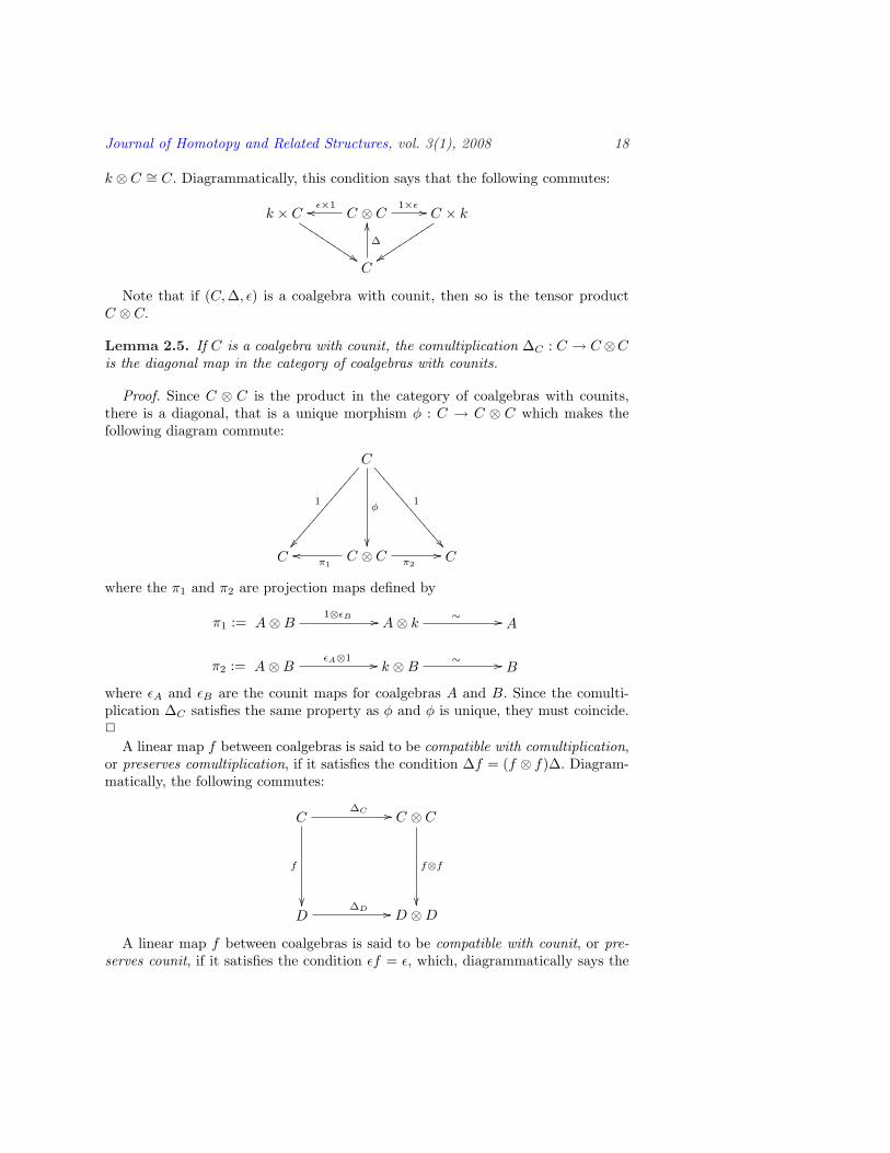
∆ : C → C ⊗C that is linear and coassociative: (∆⊗ 1)∆ = (1⊗∆)∆. A coalgebrais cocommutative if the comultiplication satisfies τ∆ = ∆, where τ : C⊗C → C⊗Cis the transposition τ(x ⊗ y) = y ⊗ x. A coalgebra with counit is a coalgebra witha linear map called the counit ε : C → k such that (ε ⊗ 1)∆ = 1 = (1 ⊗ ε)∆ via



k ⊗ C ∼= C. Diagrammatically, this condition says that the following commutes:

k × C

$$JJJJJJJJJJ C ⊗ Cε×1oo 1×ε // C × k

zztttttttttt

C

∆

OO

Note that if (C, ∆, ε) is a coalgebra with counit, then so is the tensor productC ⊗ C.

Lemma 2.5. If C is a coalgebra with counit, the comultiplication ∆C : C → C⊗Cis the diagonal map in the category of coalgebras with counits.

Proof. Since C ⊗ C is the product in the category of coalgebras with counits,there is a diagonal, that is a unique morphism φ : C → C ⊗ C which makes thefollowing diagram commute:

C

1

¢¢¤¤¤¤

¤¤¤¤

¤¤¤¤

¤¤¤

φ

²²

1

ÀÀ;;;

;;;;

;;;;

;;;;

C C ⊗ Cπ1oo

π2// C

where the π1 and π2 are projection maps defined by

π1 := A⊗B1⊗εB // A⊗ k

∼ // A

π2 := A⊗BεA⊗1 // k ⊗B

∼ // B

where εA and εB are the counit maps for coalgebras A and B. Since the comulti-plication ∆C satisfies the same property as φ and φ is unique, they must coincide.2

A linear map f between coalgebras is said to be compatible with comultiplication,or preserves comultiplication, if it satisfies the condition ∆f = (f ⊗ f)∆. Diagram-matically, the following commutes:

C∆C //

f

²²

C ⊗ C

f⊗f

²²D

∆D // D ⊗D

A linear map f between coalgebras is said to be compatible with counit, or pre-serves counit, if it satisfies the condition εf = ε, which, diagrammatically says the



following diagram commutes:

CεC //

f ÃÃ@@@

@@@@

k

D

εD

OO

In particular, if (C, ∆, ε) is a coalgebra with counit, a linear map q : C ⊗C → Cbetween coalgebras is compatible with comultiplication if and only if it satisfies∆q = (q ⊗ q)(1 ⊗ τ ⊗ 1)(∆ ⊗∆), and it is compatible with counit if and only if itsatisfies εq = q(ε⊗ ε).

A morphism f in the category of coalgebras with counit is a linear map thatpreserves comultiplication and counit. As suggested by the categories listed in Re-mark 2.4, we will focus our main attention on coalgebras with counits. Thus, we usethe word ‘coalgebra’ to refer to a coalgebra with counit and the phrase ‘coalgebramorphism’ to refer to a linear map that preserves comultiplication and counit. Onthe other hand, we wish to consider examples in which the self-distributive mapis not compatible with the counit (see the sequel). For categorical hygiene, we aredistinguishing a function that satisfies self-distributivity and is compatible withcomultiplication from a morphism in the category Coalg.

3. Self-Distributive Maps for Coalgebras

In this section we give concrete and broad examples of self-distributive mapsfor cocommutative coalgebras. Specifically, we discuss examples constructed fromquandles/racks used as bases, Lie algebras, and Hopf algebras.

3.1. Self-Distributive Maps for Coalgebras Constructed From RacksIn this section we note that quandles and racks can be used to construct self-

distributive maps in CoComCoalg simply by using their elements as basis.Let X be a rack. Let V = kX be the vector space over a field k with the

elements of X as basis. Then V is a cocommutative coalgebra with counit, withcomultiplication ∆ induced by the diagonal map ∆(x) = x ⊗ x, and the counitinduced by ε(x) = 1 for x ∈ X. This is a standard construction of a coalgebra withcounit from a set.

Set W = k ⊕ kX. We denote an element of W = k ⊕ kX by a +∑

x∈X axx ormore briefly by a+

∑x axx, and when context is understood by a+

∑axx. Extend

∆ and ε on V = kX to W by linearly extending ∆(1) = 1 ⊗ 1 and ε(1) = 1 for1 ∈ k. More explicitly,

∆(a +∑

axx) = a(1⊗ 1) +∑

ax(x⊗ x),

and ε(a +∑

axx) = a +∑

ax. With these definitions, one can check that (W,∆, ε)is an object in CoComCoalg.

Define q : W ⊗ W → W by linearly extending q(x ⊗ y) = x / y, q(1 ⊗ x) = 1,



q(x⊗ 1) = 0, and q(1⊗ 1) = 0. More explicitly,

q( (a +∑

axx)⊗ (b +∑

byy) ) =∑

y

aby +∑x,y

axby(x / y).

Proposition 3.1. The extended map q given above is a self-distributive linear mapcompatible with comultiplication.

Proof. The proof is by calculations. For example, the LHS of the self-distributivityis computed as

q(q ⊗ 1)( (a +∑

axx)⊗ (b +∑

byy)⊗ (c +∑

czz) )

= q( (∑

y

aby +∑x,y

axby(x / y))⊗ (c +∑

czz) )

=∑y,z

abycz +∑x,y,z

axbycz((x / y) / z),

which is compared with the RHS. Similarly, the compatibility is proved by verifying∆q = (q ⊗ q)(1⊗ τ ⊗ 1)(∆⊗∆). 2

The pair (W, q) falls short of being a shelf in CoComCoalg due to the following:

Proposition 3.2. The extended map q defined above is not compatible with thecounit, but satisfies εq = q(ε⊗ 1).

Proof. The counit ε has as its image k ⊂ W . Thus the image of ε⊗1 is in W ⊗W .We compute the following three quantities:

εq( (a +∑

axx)⊗ (b +∑

byy) ) = ε(∑

aby +∑x,y

axby(x / y))

= a∑

by +∑x,y

axby,

ε⊗ ε( (a +∑

axx)⊗ (b +∑

byy) ) = (a +∑

ax)(b +∑

by)

= ab + a∑

by + b∑

ax +∑

axby, and

q(ε⊗ 1)( (a +∑

axx)⊗ (b +∑

byy) ) = q( (a +∑

ax)⊗ (b +∑

byy) )

= (a +∑

ax)∑

by.

The first and third coincide. 2

3.2. Lie AlgebrasA Lie algebra g is a vector space over a field k of characteristic other than 2, with

an antisymmetric bilinear form [·, ·] : g × g → g that satisfies the Jacobi identity[[x, y], z] + [[y, z], x] + [[z, x], y] = 0 for any x, y, z ∈ g. Given a Lie algebra g overk we can construct a coalgebra N = k ⊕ g. We will denote elements of N as either(a, x) or a + x, depending on clarity, where a ∈ k and x ∈ g.

In fact, N is a cocommutative coalgebra with comultiplication and counit givenby ∆(x) = x⊗ 1 + 1⊗ x for x ∈ g and ∆(1) = 1⊗ 1, ε(1) = 1, ε(x) = 0 for x ∈ g.



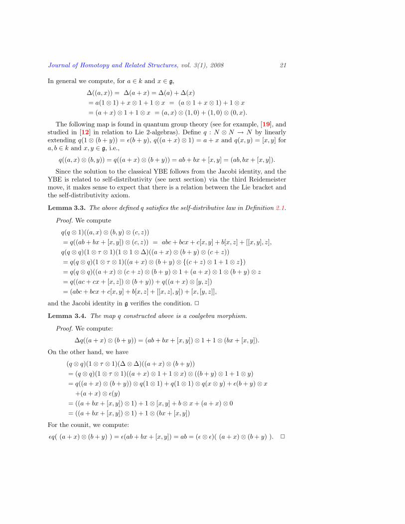
In general we compute, for a ∈ k and x ∈ g,

∆((a, x)) = ∆(a + x) = ∆(a) + ∆(x)= a(1⊗ 1) + x⊗ 1 + 1⊗ x = (a⊗ 1 + x⊗ 1) + 1⊗ x

= (a + x)⊗ 1 + 1⊗ x = (a, x)⊗ (1, 0) + (1, 0)⊗ (0, x).

The following map is found in quantum group theory (see for example, [19], andstudied in [12] in relation to Lie 2-algebras). Define q : N ⊗ N → N by linearlyextending q(1 ⊗ (b + y)) = ε(b + y), q((a + x) ⊗ 1) = a + x and q(x, y) = [x, y] fora, b ∈ k and x, y ∈ g, i.e.,

q((a, x)⊗ (b, y)) = q((a + x)⊗ (b + y)) = ab + bx + [x, y] = (ab, bx + [x, y]).

Since the solution to the classical YBE follows from the Jacobi identity, and theYBE is related to self-distributivity (see next section) via the third Reidemeistermove, it makes sense to expect that there is a relation between the Lie bracket andthe self-distributivity axiom.

Lemma 3.3. The above defined q satisfies the self-distributive law in Definition 2.1.

Proof. We compute

q(q ⊗ 1)((a, x)⊗ (b, y)⊗ (c, z))= q((ab + bx + [x, y])⊗ (c, z)) = abc + bcx + c[x, y] + b[x, z] + [[x, y], z],q(q ⊗ q)(1⊗ τ ⊗ 1)(1⊗ 1⊗∆)((a + x)⊗ (b + y)⊗ (c + z))= q(q ⊗ q)(1⊗ τ ⊗ 1)((a + x)⊗ (b + y)⊗ {(c + z)⊗ 1 + 1⊗ z})= q(q ⊗ q)((a + x)⊗ (c + z)⊗ (b + y)⊗ 1 + (a + x)⊗ 1⊗ (b + y)⊗ z

= q((ac + cx + [x, z])⊗ (b + y)) + q((a + x)⊗ [y, z])= (abc + bcx + c[x, y] + b[x, z] + [[x, z], y]) + [x, [y, z]],

and the Jacobi identity in g verifies the condition. 2

Lemma 3.4. The map q constructed above is a coalgebra morphism.

Proof. We compute:

∆q((a + x)⊗ (b + y)) = (ab + bx + [x, y])⊗ 1 + 1⊗ (bx + [x, y]).

On the other hand, we have

(q ⊗ q)(1⊗ τ ⊗ 1)(∆⊗∆)((a + x)⊗ (b + y))= (q ⊗ q)(1⊗ τ ⊗ 1)((a + x)⊗ 1 + 1⊗ x)⊗ ((b + y)⊗ 1 + 1⊗ y)= q((a + x)⊗ (b + y))⊗ q(1⊗ 1) + q(1⊗ 1)⊗ q(x⊗ y) + ε(b + y)⊗ x

+(a + x)⊗ ε(y)= ((a + bx + [x, y])⊗ 1) + 1⊗ [x, y] + b⊗ x + (a + x)⊗ 0= ((a + bx + [x, y])⊗ 1) + 1⊗ (bx + [x, y])

For the counit, we compute:

εq( (a + x)⊗ (b + y) ) = ε(ab + bx + [x, y]) = ab = (ε⊗ ε)( (a + x)⊗ (b + y) ). 2



Combining these two lemmas, we have:

Proposition 3.5. The coalgebra N together with map q given above defines a shelf(N, q) in CoComCoalg.

Groups have quandle structures given by conjugation, and their subcategory ofLie groups are related to Lie algebras through tangent spaces and exponential maps.In the above proposition we constructed shelves in CoComCoalg from Lie algebras,so we see this proposition as a step in completing the following square of relations.

Lie groups //

²²

Lie algebras

²²Quandles // ???

3.3. Hopf Algebras

A bialgebra is an algebra A over a field k together with a linear map called theunit η : k → A, satisfying η(a) = a1 where 1 ∈ A is the multiplicative identityand with an associative multiplication µ : A ⊗ A → A that is also a coalgebrasuch that the comultiplication ∆ is an algebra homomorphism. A Hopf algebrais a bialgebra C together with a map called the antipode S : C → C such thatµ(S ⊗ 1)∆ = ηε = µ(1⊗ S)∆, where ε is the counit.

The reader can construct commutative diagrams similar to those found in Section2.3 for the notions of bialgebra and Hopf algebra. Our diagrammatic conventions forthese maps are depicted in Fig. 2. Recall that the diagrams are read from bottomto top. These diagrams have been used (see for example [18, 27]) for proving factsabout Hopf algebras and related invariants.

We review the diagrammatic representation of Hopf algebra axioms. For conve-nience, assume that the underlying vector space of A is finite dimensional with or-dered basis (e1, e2, . . . , en). Then the multiplication µ and comultiplication ∆ are de-termined by the values, Λ`

ij , Yij` ∈ k, of the structure constants: µ(ei⊗ej) = Λ`

ij(e`),and ∆(e`) = Y ij

` ei ⊗ ej . Note that summation conventions are being applied, andso, for example, Λ`

ij(e`) =∑n

`=1 Λ`ij(e`). Similarly, the unit can be written as

η(1) =∑

i Aiei. The co-unit can be written as ε(ei) = Vi ∈ k, so that for a generalvector,

∑i αiei, we have ε(

∑αiei) = (

∑i Ai)ε(ei) =

∑i aiVi. Finally, the antipode

is a linear map so S(ei) = sjiej for constants sj

i ∈ k.

Thus the axioms of a (finite dimensional) Hopf algebra can be formulated in termsof the structure constants. The table below summarizes these formulations. Againsummation convention applies, and all super, and subscripted letters are constantsin the ground field.



associativity ΛqirΛ

rj` = Λq

p`Λpij

coassociativity Y ijp Y p`

q = Y j`r Y ir

q

unit Λ`ijA

j = AjΛ`ji = δ`

i

co-unit V iY ij` = Y ji

` Vi = δj`

Compatibility ΛptvΛ

quwY tu

i Y vwj = Y pq

r Λrij

Antipode Λirqs

rpY

pqj = Λi

rqsqpY

rpj = ViA

j

In the table above, δ`i denotes a Kronecker delta function. It is a small step

now to translate these. Specifically, the multiplication tensor Λ is diagrammaticallyrepresented by the leftmost trivalent vertex read from bottom to top. The letterchoices Λ, Y , A and V are meant to suggest the graphical depictions of theseoperators. A composition of maps corresponds to a contraction of the correspondingindices of tensors which, in turn, corresponds to connecting end points of diagramstogether vertically. Figures 2 and 3 represent such diagrammatic conventions ofmaps that appear in the definition of a Hopf algebra and their axioms. The gap inthe ‘Antipode condition’ diagram in Fig. 3 should be interpreted as follows: Thecounit results in a constant which is then reimbedded in the algebra via the unitmap.

xy

x

∆

x x(1) (2)

ε

ηµ

xS( )

x x y

τ

xy

ComultiplicationMultiplication Unit Counit Antipode Transposition

x y

S

Figure 2: Operations in Hopf algebras

Associativity

Unit Counit Counit is an algebra hom

CompatibilityCoassociativity

Antipode conditionUnit is a coalgebra hom

S S

Figure 3: Axioms of Hopf algebras

Let H be a Hopf algebra. Define q : H ⊗ H → H by q = µ(1 ⊗ µ)(S ⊗ 1 ⊗1)(τ ⊗ 1)(1 ⊗ ∆) where µ, ∆, and S denote the multiplication, comultiplication,



and antipode, respectively. If we adopt the common notation ∆(x) = x(1) ⊗ x(2)

and µ(x ⊗ y) = xy, then q is written as q(x ⊗ y) = S(y(1))xy(2). This appearsas an adjoint map in [26, 20], and its diagram is depicted in Fig. 4. Notice theanalogy with the group conjugation as a quandle: in a group ring, ∆(y) = y ⊗ yand S(y) = y−1, so that q(x⊗ y) = y−1xy, and therefore, is of a great interest frompoint of view of quandles.

S

Figure 4: Self-distributive map in Hopf algebras

Figure 5: Proof of self-distributivity in Hopf algebras

Proposition 3.6. The above defined linear map q : H ⊗ H → H satisfies theself-distributive law in Definition 2.1.

Proof. In Fig. 5, it is indicated that this follows from two properties of the adjointmap: q(q ⊗ 1) = q(1⊗ µ) (which is used in the first and the third equalities in thefigure), and µ = µ(1⊗ q)(τ ⊗ 1)(1⊗∆) (which is used in the second equality).

It is known that these properties are satisfied, and proofs are found in [26, 15].Here we include diagrammatic proofs for the reader’s convenience in Fig. 6 andFig. 7, respectively. The dotted loops in Fig. 6, and all those that follow, indicatewhere changes are made to the diagram. 2

Remark 3.7. The definition of q above contains an antipode, which is a coalgebraanti-homomorphism and not necessarily a coalgebra morphism. Thus, (H, q) is nota shelf in Coalg in general.

3.4. Other ExamplesIn this section we observe that there are plenty of examples of self-distributive lin-

ear maps for 2-dimensional cocommutative coalgebras and shelves in CoComCoalg.Let V be the two dimensional vector space over k with basis {x, y}. Define a

coalgebra structure on V using the diagonal map ∆(z) = z ⊗ z for z ∈ {x, y} andextending it linearly.



Anti−hom.

Associativity Assoc.

NaturalityCompatibility

Cancel

Assoc.

S

S

S S

S

S

S SS

S

Figure 6: q(q ⊗ 1) = q(1⊗ µ)

SS

Figure 7: µ = µ(1⊗ q)(τ ⊗ 1)(1⊗∆)

Lemma 3.8. A linear map q : V ⊗ V → V is self-distributive and compatible withcomultiplication if and only if q is one of the functions indicated via any columnin the table below. The values are determined on the basis elements x⊗ x, throughy ⊗ y as indicated.

q(x⊗ x) = 0 0 0 0 0 0 x x x x x x x x x y y y y y 0q(x⊗ y) = 0 0 0 0 x y 0 0 0 x x x x y y 0 x y y y 0q(y ⊗ x) = 0 0 x x 0 0 0 0 y x x y y x y 0 y 0 x y 0q(y ⊗ y) = x y 0 x y 0 0 y 0 x y x y y y 0 y 0 x y 0

Among these, (V, q) is a shelf in CoComCoalg if and only if q(a, b) 6= 0 for anya, b ∈ {x, y}.

Proof. Let q(x⊗x) = γ1x+γ2y for some constants γ1, γ2 ∈ k. The compatibilitycondition

∆q(x⊗ x) = (q ⊗ q)(1⊗ τ ⊗ 1)(∆⊗∆)(x⊗ x)

implies that γ1γ2 = 0 and γ21 = γ1, γ2

2 = γ2, i.e., q(x ⊗ x) = 0, x, or y. The sameholds for x⊗ y, y ⊗ x and y ⊗ y, so that the value of q for a pair of basis elementsis either a basis element (x or y), or 0.



A case by case analysis (facilitated by Mathematica and/or Maple) providesself-distributivity. When ε(x) = ε(y) = 1, the only cases for which εq = ε ⊗ ε arethose for which q(a, b) 6= 0 for all four choices of a, b. 2

Another famous example of a cocommutative coalgebra is the trigonometric coal-gebra, T , generated by a and b with comultiplication given by:

∆(a) = a⊗ a− b⊗ b

∆(b) = a⊗ b + b⊗ a

with counit ε(a) = 1, ε(b) = 0, in analogy with formulas for cos(x+y) and sin(x+y)and cos(0) = 1, sin(0) = 0.

Lemma 3.9. Let T denote the trigonometric coalgebra over C. Let q : T ⊗ T → Tbe a linear map defined by:

q(a⊗ a) = α1a + β1b,q(a⊗ b) = α2a + β2b,

q(b⊗ a) = α3a + β3b,q(b⊗ b) = α4a + β4b.

Then such a linear map q is self-distributive and compatible with comultiplication ifand only if the coefficients are found in Table 1, where i =

√−1.Among these, (V, q) is a shelf in CoComCoalg if and only if (α1, α2, α3, α4) =

(1, 0, 0, 0).

Proof. This result is a matter of verifying the conditions for self-distributivityand compatibility over all possible choices of inputs. We generated solutions byboth Maple and Mathematica. For the compatibility condition we established asystem of 12 quadratic equations in eight unknowns. Originally there were 16 suchequations, but 4 of these are duplicates. In the Mathematica program we used thecommand “Solve” to generate a set of necessary conditions. The self-distributivecondition gave a system of cubic equations in the unknowns. We checked thesesubject to the necessary conditions, and found the 21 solutions above.

Expressing ε as a (1×2) matrix and q as the 2×4 matrix(

α1 α2 α3 α4

β1 β2 β3 β4

).

We compute εq = (α1, α2, α3, α4) and ε⊗ ε = (1, 0, 0, 0). The result follows. 2

4. Yang–Baxter Equation and Self-Distributive Maps for Co-algebras

In this section, we discuss relationships between solutions to the Yang-Baxterequations and self-distributive maps.

4.1. A Brief Review of YBEThe Yang–Baxter equation makes sense in any monoidal category. Originally

mathematical physicists concentrated on solutions in the category of vector spaceswith the tensor product, obtaining solutions from quantum groups.

Let V be a vector space and R : V ⊗ V → V ⊗ V an invertible linear map. Wesay R is a Yang–Baxter operator if it satisfies the Yang–Baxter equation, (YBE),



α1 α2 α3 α4 β1 β2 β3 β4

1 0 0 0 0 0 −1 00 0 0 0 0 0 0 012 − i

2 0 0 0 0 12 − i

212

i2 0 0 0 0 1

2i2

1 0 0 0 0 0 1 012 0 0 − 1

2 0 12

12 0

1 0 0 0 0 1 0 014 − i

4 − i4 − 1

4 − i4 − 1

4 − 14

i4

14

i4 − i

414 − i

414 − 1

4 − i4

14

i4

i4 − 1

4 − i4

14

14

i4

14

i4

i4 − 1

4i4 − 1

4 − 14 − i

414 − i

4i4

14

i4

14 − 1

4i4

14 − i

4 − i4 − 1

4i4

14

14 − i

4

1 0 0 0 − i2 − 1

212

i2

12 0 − i

2 0 − i2 0 − 1

2 01 0 0 0 − i

212

12 − i

2

1 0 0 0 i2 − 1

212 − i

212 0 i

2 0 i2 0 − 1

2 01 0 0 0 i

212

12

i2

1 0 0 0 −i 0 0 01 0 0 0 i 0 0 0

Table 1: List of self-distributive maps in the trigonometric coalgebra

which says that: (R ⊗ 1)(1 ⊗ R)(R ⊗ 1) = (1 ⊗ R)(R ⊗ 1)(1 ⊗ R). In other words,the YBE says that the following diagram commutes:

V ⊗ V ⊗ V

V ⊗ V ⊗ V

V ⊗ V ⊗ V

V ⊗ V ⊗ V

V ⊗ V ⊗ V

V ⊗ V ⊗ V

R⊗1

**UUUUUUUUUU1⊗R

uujjjjjjjjj

R⊗1

²²

1⊗R ))TTTTTTTTT

R⊗1ttiiiiiiiiii

1⊗R

²²

A solution to the YBE is also called a braiding.

In general, a braiding operation provides a diagrammatic description of the pro-cess of switching the order of two things. This idea is formalized in the concept of



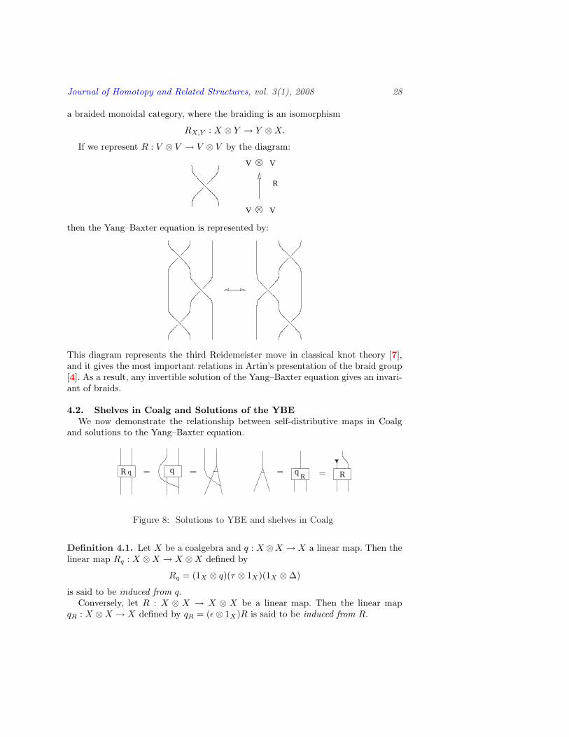
a braided monoidal category, where the braiding is an isomorphism

RX,Y : X ⊗ Y → Y ⊗X.

If we represent R : V ⊗ V → V ⊗ V by the diagram:

V V

V V

R

then the Yang–Baxter equation is represented by:

This diagram represents the third Reidemeister move in classical knot theory [7],and it gives the most important relations in Artin’s presentation of the braid group[4]. As a result, any invertible solution of the Yang–Baxter equation gives an invari-ant of braids.

4.2. Shelves in Coalg and Solutions of the YBEWe now demonstrate the relationship between self-distributive maps in Coalg

and solutions to the Yang–Baxter equation.

RqR q q R

Figure 8: Solutions to YBE and shelves in Coalg

Definition 4.1. Let X be a coalgebra and q : X ⊗X → X a linear map. Then thelinear map Rq : X ⊗X → X ⊗X defined by

Rq = (1X ⊗ q)(τ ⊗ 1X)(1X ⊗∆)

is said to be induced from q.Conversely, let R : X ⊗ X → X ⊗ X be a linear map. Then the linear map

qR : X ⊗X → X defined by qR = (ε⊗ 1X)R is said to be induced from R.



RRR

Figure 9: Hypotheses of Theorem 4.2

R

R R

R

R

R

R

R

R

R

R

Figure 10: Proof of Theorem 4.2

Diagrammatically, constructions of one of these maps from the other are depictedin Fig. 8. Our goal is to relate solutions of the YBE and self-distributive maps incertain categories via these induced maps.

Theorem 4.2. Let R : X ⊗X → X ⊗X be a solution to the YBE on a coalgebraX with counit. Suppose R satisfies (ε ⊗ ε)R = (ε ⊗ ε) and RqR

= R. Then (X, qR)is a shelf in Coalg.

Proof. The conditions in the assumption are presented in Fig. 9. A proof ispresented in Fig. 10. 2

Theorem 4.3. Let X be an object in CoComCoalg. Suppose a self-distributivelinear map q : X ⊗ X → X is compatible with comultiplication. Then Rq is asolution to the YBE.

Proof. The cocommutativity of ∆ is depicted in Fig. 11. A proof, then, is depictedin Fig. 12. Note here the condition that q is compatible with comultiplication is:

Co-commut.

Figure 11: Cocommutativity



Compati−bility

Self−distributivityCocommutativityNaturality

Naturality Cocommutativity CoassociativityNaturality

NaturalityAssoc. Naturality Naturality

Coassociativity

Figure 12: Proof of Theorem 4.3

∆(q(a⊗b)) = q(a(1)⊗b(1))⊗q(a(2)⊗b(2)) or, equivalently, ∆q = q(1⊗τ⊗1)(∆⊗∆).This is applied in Fig. 12 on the bottom row with the equal sign indicated to followfrom compatibility. 2

Propositions 3.1 and 3.5 and Theorem 4.3 imply the following:

Corollary 4.4. Let q be a map defined from a quandle/rack as in Proposition 3.1or from a Lie algebra as in Proposition 3.5. Then the induced map Rq is a solutionto the YBE.

In the Lie algebra case, the map is given as follows:

Rq((a, x)⊗ (b, y)) = (b, y)⊗ (a, x) + (1, 0)⊗ (0, [x, y]).

This appears, for example, in [12, 19].

Remark 4.5. Next we focus on the case of the adjoint map in Hopf algebras.Remark 3.7 states that the self-distributive map q(x ⊗ y) = S(y(1))xy(2) is notcompatible with comultiplication, and therefore, Theorem 4.3 cannot be applied.However, the induced map Rq does, indeed, satisfy the YBE. This is of course for



Figure 13: Conclusion of Prop. 4.6/ Hypothesis of Prop. 4.7

Def.

Counit

UnitDef.

antip.

compat.

Redraw

Counit

Unit

co-assoc.

assoc.assoc.

co-assoc.co-assoc.

antipode

compatiblity

assoc.

NaturalityCo-assoc.

S

S

S

S

S

S

SS

S

S S

S

S

S

S

S

S

Figure 14: Proof of Proposition 4.6, second equation

different reasons, and proved in [26], which was interpreted in [15] as a restriction ofa regular representation of the universal R-matrix of a quantum double. Since it isof a great interest why the same construction gives rise to solutions to the YBE fordifferent reasons, we include their proofs in diagrams for the reader’s convenience,and we specify two conditions from [26] in our point of view, to construct Rq fromq, and make a restatement of a theorem in [26] as follows:

Proposition 4.6. In a Hopf algebra, let q = µ(1 ⊗ µ)(S ⊗ 1 ⊗ 1)(τ ⊗ 1)(1 ⊗ ∆).Then q(q⊗ 1) = q(1⊗µ) and (q⊗µ)(1⊗ τ ⊗ 1)(∆⊗∆) = (1⊗µ)(τ ⊗ 1)(1⊗∆)(1⊗q)(τ ⊗ 1)(1⊗∆).

Proof. The proofs are indicated in Figs. 6 and 14, respectively. 2

Recall from Section 3.3 that in a Hopf algebra, the map q = µ(1 ⊗ µ)(S ⊗ 1 ⊗1)(τ ⊗ 1)(1⊗∆) satisfies self-distributivity.

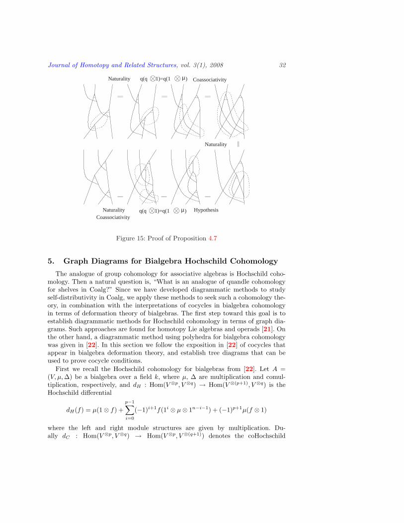
Proposition 4.7. Suppose X is a Hopf algebra and q is any linear map that satisfiesq(q ⊗ 1) = q(1 ⊗ µ) and (q ⊗ µ)(1 ⊗ τ ⊗ 1)(∆ ⊗ ∆) = (1 ⊗ µ)(τ ⊗ 1)(1 ⊗ ∆)(1 ⊗q)(τ ⊗ 1)(1⊗∆). Then Rq is a solution to the YBE.

Proof. The required conditions are depicted in Fig. 13. And the proof is given inFig. 15. 2

In particular, the above proposition applies when q(x⊗ y) = S(y(1))xy(2).



Naturality Coassociativity

Naturality

HypothesisNaturalityCoassociativity

µ

µq(q 1)=q(1 )

q(q 1)=q(1 )

Figure 15: Proof of Proposition 4.7

5. Graph Diagrams for Bialgebra Hochschild Cohomology

The analogue of group cohomology for associative algebras is Hochschild coho-mology. Then a natural question is, “What is an analogue of quandle cohomologyfor shelves in Coalg?” Since we have developed diagrammatic methods to studyself-distributivity in Coalg, we apply these methods to seek such a cohomology the-ory, in combination with the interpretations of cocycles in bialgebra cohomologyin terms of deformation theory of bialgebras. The first step toward this goal is toestablish diagrammatic methods for Hochschild cohomology in terms of graph dia-grams. Such approaches are found for homotopy Lie algebras and operads [21]. Onthe other hand, a diagrammatic method using polyhedra for bialgebra cohomologywas given in [22]. In this section we follow the exposition in [22] of cocycles thatappear in bialgebra deformation theory, and establish tree diagrams that can beused to prove cocycle conditions.

First we recall the Hochschild cohomology for bialgebras from [22]. Let A =(V, µ, ∆) be a bialgebra over a field k, where µ, ∆ are multiplication and comul-tiplication, respectively, and dH : Hom(V ⊗p, V ⊗q) → Hom(V ⊗(p+1), V ⊗q) is theHochschild differential

dH(f) = µ(1⊗ f) +p−1∑

i=0

(−1)i+1f(1i ⊗ µ⊗ 1n−i−1) + (−1)p+1µ(f ⊗ 1)

where the left and right module structures are given by multiplication. Du-ally dC : Hom(V ⊗p, V ⊗q) → Hom(V ⊗p, V ⊗(q+1)) denotes the coHochschild



differential. These define the total complex (C∗b (A;A), D), where Cnb (A; A) =

⊕ni=1Hom(V ⊗(n−i+1), V ⊗i). For example, for a 1-cochain f ∈ Hom(V, V ), dH(f)(x⊗

y) = xf(y) − f(xy) + f(x)y and dC(f)(x) = x(1) ⊗ f(x(2)) − f(x)(1) ⊗ f(x)(2) +f(x(1))⊗ x(2).

For the rest of this section, we establish graph diagrams for Hochschild cohomol-ogy and review their aspects in deformation theory of bialgebras.

5.1. Graph Diagrams for Hochschild DifferentialsA 1-cochain f ∈ Hom(V, V ) is represented by a circle on a vertical segment as

shown in Fig. 16, where the images of f under the first differentials dH(f) anddC(f), as computed above, are also depicted. In general, a (m + n − 1)-cochain inHom(V ⊗m, V ⊗n) is represented by a diagram in Fig. 17.

( ) =H + dC+

,( ) =d

Figure 16: Hochschild 1-differentials

n

m

Figure 17: Hochschild (m + n)-cochains

Let τ be the transposition. In general, τi indicates the transposition of the ithand (i + 1)st factors; the notation is used when type-setting gets complicated. For(φ1, φ2), where φ1 ∈ Hom(V ⊗2, V ) and φ2 ∈ Hom(V, V ⊗2), the differentials are

dH(φ1) = µ(1⊗ φ1)− φ1(µ⊗ 1) + φ1(1⊗ µ)− µ(φ1 ⊗ 1), (1)dC(φ1) = (µ⊗ φ1)τ2(∆⊗∆)−∆(φ1) + (φ1 ⊗ µ)τ2(∆⊗∆), (2)dH(φ2) = (µ⊗ µ)τ2(∆⊗ φ2)− φ2µ + (µ⊗ µ)τ2(φ2 ⊗∆), (3)dC(φ2) = (1⊗ φ2)∆− (∆⊗ 1)(φ2) + (1⊗∆)(φ2)− (φ2 ⊗ 1)∆. (4)

The 2-cocycle conditions are dH(φ1) = 0, dC(φ1) = dH(φ2), and dC(φ2) = 0. Thedifferential D of the total complex is D = dH−dC , D(φ1, φ2) = dH(φ1)+[dH(φ2)−dC(φ1)]− dC(φ2).

We demonstrate a proof that (φ1, φ2) = (dH(f), dC(f)) satisfies dC(φ1) = dH(φ2)using graph diagrams. First, we use encircled vertices as depicted in Fig. 17 to rep-resent an element of Hom(V ⊗m, V ⊗n). Then dC(φ1) and dH(φ2) are represented onthe top line of Fig. 18. Substituting (φ1, φ2) = (dH(f), dC(f)), that are represented



=

d ( ) =

=

Hd

C( ) =

Figure 18: Hochschild 2-differentials

diagrammatically as in Fig. 16, we perform diagrammatic computations as in therest of Fig. 18, and the equality follows because multiplication and comultiplicationare compatible. In particular each diagram in the left of the figure for which thevertex is external to the operations corresponds to a similar diagram on the right,but the correspondence is given after considering the compatible structures.

0

Figure 19: Hochschild 3-cocycle conditions

For 3-cochains ψi ∈ Hom(V ⊗3, V ), ψ2 ∈ Hom(V ⊗2, V ⊗2) and ψ3 ∈ Hom(V, V ⊗3),the 3-cocycle condition is explicitly written as dH(ψ1) = 0, dC(ψ1) = dH(ψ2),dC(ψ2) = dH(ψ3), and dC(ψ3) = 0, see [22]

dH(ψ1) = µ(1⊗ ψ1)− ψ1(µ⊗ 12) + ψ1(1⊗ µ⊗ 1)− ψ1(12 ⊗ µ) + µ(ψ1 ⊗ 1),dC(ψ1) = (µ(1⊗ µ)⊗ ψ1)τ(∆⊗∆⊗∆)−∆(ψ1) + (ψ1 ⊗ µ(µ⊗ 1))τ(∆⊗∆⊗∆),dH(ψ2) = (µ⊗ µ)τ2(∆⊗ ψ2)− ψ2(µ⊗ 1) + ψ2(1⊗ µ)− (µ⊗ µ)τ2(ψ2 ⊗∆),dC(ψ2) = (µ⊗ ψ2)τ2(∆⊗∆)− (∆⊗ 1)(ψ2) + (1⊗∆)(ψ2)− (ψ2 ⊗ µ)τ2(∆⊗∆),dH(ψ3) = (µ⊗ µ⊗ µ)τ ′((1⊗∆)∆⊗ ψ3)− ψ3(µ) + (µ⊗ µ⊗ µ)τ ′(ψ3 ⊗ (∆⊗ 1)∆),dC(ψ3) = (1⊗ ψ3)∆− (∆⊗ 12)(ψ3) + (1⊗∆⊗ 1)(ψ3)− (12 ⊗∆)(ψ3) + (ψ3 ⊗ 1)∆,



where τ = τ4τ3τ2 and τ ′ = τ5τ2τ3.The first two 3-cocycle conditions, dH(ψ1) = 0 and dC(ψ1) = dH(ψ2), are de-

picted in Fig. 19. Note that the first is the pentagon identity for associativity. Inparticular, ψ1 can be regarded as an obstruction to associativity. The morphismψ1 is assigned the difference between the two diagrams that represent the two ex-pressions (ab)c and a(bc). Thus ψ1 and its diagram are assigned to the change ofdiagrams corresponding to associativity, and can be seen to form an actual pen-tagon, as depicted in Fig. 20.

In Fig. 20 the usual pentagon relation is depicted and adorned. Consider, forexample, the graph at the top of the pentagon (which corresponds to the associ-ated string ((ab)c)d) and its descendent on the far left (which corresponds to theassociated string (a(bc))d). The top left arrow that represents the parentheticalregrouping is decorated by a graph (encircled by a dotted arc) with a Neptune’strident on the lower left. The solid circle at the trident’s junction represents a 3-cocycle. The trident, then, corresponds to the unassociated string abc. The dottedencircling of graphs with tridents is given to indicate that these correspond to thearrows of the pentagon relation. The 3-cocycle condition is written so that the sumof the three cochains on the left of the figure is equal to the sum of the two on theright.

In general, when graph transformations are given the arrows are denoted bygraphs encircled by dotted arcs and with distinguished (singular) vertices indicatedby solid colors or solid circles at the vertex.

Figure 20: Hochschild 3-cocycles as movies, part I

Similarly, the second condition dC(ψ1) = dH(ψ2) can be represented as a se-quence of applications of the associativity and compatibility conditions as depictedin Fig. 21. Furthermore, the relations dC(ψ2) = dH(ψ3) and dC(ψ3) = 0 can beobtained by turning the equations in Fig. 19 upside-down. Similarly, the “movie-moves” in Figs. 20 and 21 can be turned upside-down. Thus, dC(ψ3) = 0 when the



pentagon identity for coassociativity holds, and dC(ψ2) = dH(ψ3) when compati-bility and coassociativity are compared.

Figure 21: Hochschild 3-cocycles as movies, part Il

5.2. Review of Cocycles in Deformation TheoryNext we follow [22] for deformation of bialgebras. A deformation of A = (V, µ, ∆)

is a k[[t]]-bialgebra At = (Vt, µt,∆t), where Vt = V ⊗ k[[t]] and At/(tAt) ∼= A.Deformations of µ and ∆ are given by µt = µ+ tµ1 + · · ·+ tnµn + · · · : Vt⊗Vt → Vt

and ∆t = ∆ + t∆1 + · · · + tn∆n + · · · : Vt → Vt ⊗ Vt where µi : V ⊗ V → V ,∆i : V → V ⊗ V , i = 1, 2, · · ·, are sequences of maps. Suppose µ = µ + · · · + tnµn

and ∆ = ∆+· · ·+tn∆n satisfy the bialgebra conditions (associativity, compatibility,and coassociativity) mod tn+1, and suppose that there exist µn+1 : V ⊗ V → Vand ∆n+1 : V → V ⊗ V such that µ + tn+1µn+1 and ∆ + tn+1∆n+1 satisfy thebialgebra conditions mod tn+2. Define ψ1 ∈ Hom(V ⊗3, V ), ψ2 ∈ Hom(V ⊗2, V ⊗2),and ψ3 ∈ Hom(V, V ⊗3) by

µ(µ⊗ 1)− µ(1⊗ µ) = tn+1ψ1 mod tn+2, (5)∆µ− (µ⊗ µ)τ2(∆⊗ ∆) = tn+1ψ2 mod tn+2, (6)

(∆⊗ 1)∆− (1⊗ ∆)∆ = tn+1ψ3 mod tn+2. (7)

For the associativity of µ + tn+1µn+1 mod tn+2 we obtain:

(µ+tn+1µn+1)((µ+tn+1µn+1)⊗1)−(µ+tn+1µn+1)(1⊗(µ+tn+1µn+1)) = 0 mod tn+2



which is equivalent by degree calculations to:

dH(µn+1) = µ(1⊗ µn+1)− µn+1(µ⊗ 1) + µn+1(1⊗ µn+1)− µ(µn+1 ⊗ 1) = ψ1.

Similarly, we obtain: (ψ1, ψ2, ψ3) = D(µn+1,∆n+1). The cochains (ψ1, ψ2, ψ3), de-fined by deformations (5,6,7) then, satisfy the 3-cocycle condition D(ψ1, ψ2, ψ3) = 0.This concludes the review of deformation for the 2-cocycle conditions cited from[22].

6. Towards a Cohomology Theory for Shelves in Coalg

Let (X, q) be a coalgebra with a self-distributive linear map. In this sectionwe present low-dimensional cocycle conditions for q. We justify our cocycle condi-tions through the use of analogy with Hochschild bialgebra cohomology using dia-grammatics and the deformation theories reviewed in the preceding section. Bothanalogies are used interchangeably throughout this section, both in definitions andcomputations.

6.1. Chain GroupsFollowing the diagrammatics of the preceding section, we define shelf chain

groups, for positive integers n and i = 1, . . . , n by:

Cn,ish (X;X) = Hom(X⊗(n+1−i), X⊗i),

Cnsh(X;X) = ⊕n

i=1Cn,ish (X; X),

where the subscript ‘sh’ denotes shelf. Specifically, the chain groups in low dimen-sions of our concern are:

C1sh(X; X) = Hom(X, X),

C2sh(X; X) = Hom(X⊗2, X)⊕Hom(X,X⊗2),

C3sh(X; X) = Hom(X⊗3, X)⊕Hom(X⊗2, X⊗2)⊕Hom(X,X⊗3).

To help keep track of the chain groups and their indices, we include the diagramin Fig. 22 and the following explanation. The reader should be warned that this isnot the standard indexing of double complexes. Instead, the chain groups Cn,i arelocated at position (n + 2− i, i) in the positive quadrant of the integer lattice. Thechain groups Cj are the direct sum of the groups along lines of slope (−1). Unlikespectral sequences, the differential dn,i is defined on multiple factors (instead of asingle factor Cn,i) of Cn and has its image in the factor Cn+1,i. Hence dn,i raisesthe first subscript of the cochain groups by 1, and the second subscript indicatesthe image factor.

In the remaining sections we will define differentials that are homomorphismsbetween the chain groups:

dn,i : Cnsh(X;X) → Cn+1,i

sh (X; X)(= Hom(X⊗(n+2−i), X⊗i))

and will be defined individually for n = 1, 2, 3 and i = 1, . . . , n + 1, and

D1 = d1,1 − d1,2 : C1sh(X;X) → C2

sh(X; X),



i

C 1 C 2 C 3 C 4

1

2,11,1 3,1 4,1

2,2

3,3

3,2 4,2

4,3

1

2

3

2 3 4n+2−i

Figure 22: The lattice of chain groups and differentials

D2 = d2,1 + d2,2 + d2,3 : C2sh(X; X) → C3

sh(X; X),D3 = d3,1 + d3,2 + d3,3 + d3,4 : C3

sh(X; X) → C3sh(X; X).

6.2. First DifferentialsWe take

d1,2 : Hom(X; X)(= C1,1sh (X; X)) → Hom(X,X⊗2)(= C2,2

sh (X;X))

to be the coHochschild differential for the comultiplication d1,2(f) = (1 ⊗ f)∆ −∆f + (f ⊗ 1)∆. Again by analogy with the differential for multiplication, we take:

d1,1 : Hom(X, X)(= C1,1sh (X;X)) → Hom(X⊗2, X)(= C2,1

sh (X;X))

to be d1,1(f) = q(1⊗ f)− fq + q(f ⊗ 1). Then define D1 : C1sh(X; X) → C2

sh(X;X)by D1 = d1,1 − d1,2.

6.3. Second DifferentialsWe derive second differentials by analogy with deformation theory, and then show

that our definitions carry through in diagrammatics.Recall that the self-distributivity, compatibility, and coassociativity are written

as:

q(q ⊗ 1) = q(q ⊗ q)τ2(1⊗ 1⊗∆),∆q = (q ⊗ q)τ2(∆⊗∆),

(∆⊗ 1)∆ = (1⊗∆)∆.

where τ2 is the transposition acting on the second and third tensor factors. As beforelet Xt = X ⊗ k[[t]] and suppose we have partial deformations q = q + · · · + tnqn

and ∆ = ∆ + · · · + tn∆n satisfying the above three conditions mod tn+1, andsuppose there are qn+1 and ∆n+1 such that q+qn+1 and ∆+∆n+1 satisfy the threeconditions mod tn+2.

Setting

q(q ⊗ 1)− q(q ⊗ q)τ2(1⊗ 1⊗ ∆) = tn+1ξ1 mod tn+2,



∆q − (q ⊗ q)τ2(∆⊗ ∆) = tn+1ξ2 mod tn+2,

(∆⊗ 1)∆− (1⊗ ∆)∆ = tn+1ξ3 mod tn+2,

we obtain:

[q(qn+1 ⊗ 1) + qn+1(q ⊗ 1)]− [qn+1(q ⊗ q)τ2(1⊗ 1⊗∆)+q(qn+1 ⊗ q)τ2(1⊗ 1⊗∆) +

q(q ⊗ qn+1)τ2(1⊗ 1⊗∆) + q(q ⊗ q)τ2(1⊗ 1⊗∆n+1)] = ξ1,

[∆qn+1 + ∆n+1q]− [(qn+1 ⊗ q)τ2(∆⊗∆) + (q ⊗ qn+1)τ2(∆⊗∆)+(q ⊗ q)τ2(∆n+1 ⊗∆) + (q ⊗ q)τ2(∆⊗∆n+1)] = ξ2,

[(∆n+1 ⊗ 1)∆ + (∆⊗ 1)∆n+1]− [(1⊗∆n+1)∆ + (1⊗∆)∆n+1] = ξ3.

A natural requirement is D2(qn+1, ∆n+1) = (ξ1, ξ2, ξ3), so we will define D2 :C2

sh(X;X) → C3sh(X; X) by D2 = d2,1 + d2,2 + d2,3. Let η1 ∈ C2,1

sh (X;X)(=Hom(X⊗2, X)) and η2 ∈ C2,2

sh (X; X)(= Hom(X,X⊗2)) be cochains. Then,

d2,1(η1, η2) = [q(η1 ⊗ 1) + η1(q ⊗ 1)]− [η1(q ⊗ q)τ2(1⊗ 1⊗∆) + q(η1 ⊗ q)τ2(1⊗ 1⊗∆)

+q(q ⊗ η1)τ2(1⊗ 1⊗∆) + q(q ⊗ q)τ2(1⊗ 1⊗ η2)]d2,2(η1, η2) = [∆η1 + η2q]− [(η1 ⊗ q)τ2(∆⊗∆) + (q ⊗ η1)τ2(∆⊗∆)

+(q ⊗ q)τ2(η2 ⊗∆) + (q ⊗ q)τ2(∆⊗ η2)]d2,3(η1, η2) = [(η2 ⊗ 1)∆ + (∆⊗ 1)η2]− [(1⊗ η2)∆ + (1⊗∆)η2] .

In fact, d2,3 = dC , the same as the coHochschild 2-differential for the comultiplica-tion.

η1

η2

q ∆

Figure 23: Diagrams for 2-cochains

Figure 24: The first 2-differential d2,1

The diagrammatic conventions for q, a 2-cochain η1 ∈ Hom(X⊗2, X), and ∆, a2-cochain η2 ∈ Hom(X, X⊗2) are depicted from left to right, respectively, in Fig. 23.

The first and second differentials d2,1(η1, η2), d2,2(η1, η2) are depicted in Fig. 24and Fig. 25, respectively. Here we note that these diagrams agree with those for



Figure 25: The second 2-differential d2,2

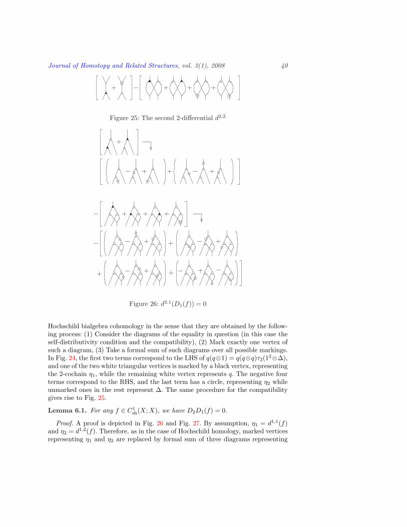
Figure 26: d2,1(D1(f)) = 0

Hochschild bialgebra cohomology in the sense that they are obtained by the follow-ing process: (1) Consider the diagrams of the equality in question (in this case theself-distributivity condition and the compatibility), (2) Mark exactly one vertex ofsuch a diagram, (3) Take a formal sum of such diagrams over all possible markings.In Fig. 24, the first two terms correspond to the LHS of q(q⊗1) = q(q⊗q)τ2(12⊗∆),and one of the two white triangular vertices is marked by a black vertex, representingthe 2-cochain η1, while the remaining white vertex represents q. The negative fourterms correspond to the RHS, and the last term has a circle, representing η2 whileunmarked ones in the rest represent ∆. The same procedure for the compatibilitygives rise to Fig. 25.

Lemma 6.1. For any f ∈ C1sh(X; X), we have D2D1(f) = 0.

Proof. A proof is depicted in Fig. 26 and Fig. 27. By assumption, η1 = d1,1(f)and η2 = d1,2(f). Therefore, as in the case of Hochschild homology, marked verticesrepresenting η1 and η2 are replaced by formal sum of three diagrams representing



Figure 27: d2,2(D1(f)) = 0

d1,1(f) and d1,2(f), see Fig. 16. The situation in which the first two terms arereplaced by three terms each is depicted in the top two lines of Fig. 26.

A white circle on an edge represents f . The bottom three lines show replacementsfor the remaining four negative terms. Then the terms represented by identicalgraphs cancel directly. If a white circle representing f appears near the boundary,then we use the self-distributive axiom to relate this to another term. For example,the first term on the top left cancels with the third term on the bottom row sincef is on the second tensor factor at the bottom of each.

To facilitate the reader’s understanding of the computation we present the fol-lowing sequences: 1,−2, 3, 4,−5, 2 and −6, 5,−7,−8, 7,−3,−9, 6,−1, 9,−4, 8. Labelthe diagrams below the arrows in Fig. 26 in order with these numbers. The mi-nus sign indicates the sign of the given term on the given side of the equation,and the number indicates which diagrams cancel which. A similar labelling can beaccomplished in Fig. 27. 2

We also note the following restricted version:

Lemma 6.2. Let f ∈ C1sh(X;X) = Hom(X; X). If d1,2(f) = 0 ∈ C2,2

sh (X; X) =Hom(X;X⊗2), then D2(d1,1(f), 0) = 0.

Proof. The conclusion is restated by the following condition: d2,i(d1,1(f), 0) =0 for i = 1, 2, since d1,1(f) is not in the domain of the differential d2,3. Thenone computes d2,i(η1, 0) for η1 = d1,1(f) either directly, or diagrammatically usingFigs. 26, and 27, without trivalent vertices that are encircled. 2



6.4. Third DifferentialsThroughout this section, we consider only self-distributive linear maps for co-

commutative coalgebras with counits. The map q needs not be compatible withthe counit (cf. Proposition 3.2), but there must be such a counit present becausesometimes the diagonal has to be defined in a categorical context. In any case,3-differentials

d3,i : C3sh(X;X)(= ⊕3

j=1Hom(X⊗(4−j), X⊗j)) →

C4,ish (X; X)(= Hom(X⊗(n+2−i), X⊗i))

are defined in Appendix AppendixA, for i = 1, 2, 3. For i = 4, it is defined bythe same map as the differential for ∆ for co-Hochschild cohomology (the pentagonidentity for the comultiplication). These differentials are defined by direct analogueswith Hochschild differentials in diagrammatics, and we will justify our definition intwo more ways: (1) 2-cochains vanish under these maps, (2) 3-cocycles of quandleand Lie algebra cohomology are realized in these formulas as discussed in the nextsection. The defining formulas and diagrammatic methods to derive them are de-ferred to Appendix AppendixA, and we proceed with statements of lemmas we needto continue with this cohomology theory.

Lemma 6.3. Let (η1, 0) ∈ Hom(X⊗2, X) ⊂ C2sh(X; X) (so that η2 = 0). Then

d3,iD2(η1, 0) = 0 for i = 1, 2, 3.

Proof and diagrams are included in Appendix AppendixB.

6.5. Cohomology GroupsNow we use these differentials to define cohomology groups for self-distributive

linear maps for objects in Coalg. Let (X, ∆) be an object in Coalg, and q : X⊗X →X be a self-distributive linear map. Then Lemmas 6.1 implies

Corollary 6.4. 0 → C1sh(X; X) D1→ C2

sh(X; X) D2→ C3sh(X;X) is a chain complex.

This enables us to define the following cohomology related groups:

Definition 6.5. The 1-cocycle and cohomology groups are defined by:

H1,ish (X;X) = Z1,i

sh (X;X) = {f ∈ C1,ish (X; X) | d1,i(f) = 0}

for i = 1, 2, andH1

sh(X; X) = Z1,1sh (X; X)⊕ Z1,2

sh (X; X).

For dimension 2, we define Z2sh(X; X) = Ker(D2), B2

sh(X;X) = Im(D1), andH2

sh(X;X) = Z2sh(X;X)/B2

sh(X; X).

Since the 2-cocycle conditions were formulated directly from a deformation theoryformulation, we have the following:

Proposition 6.6. Let Xt = X ⊗ k[[t]] and suppose we have partial deformationsq = q + · · · + tnqn and ∆ = ∆ + · · · + tn∆n satisfying the above three conditions



mod tn+1, so that they define a self-distributive map in Coalg mod tn+1. Then thereexist qn+1 : X ⊗ X → X and ∆n+1 : X → X ⊗ X such that q + tn+1qn+1 and∆ + tn+1∆n+1 satisfy the three conditions mod tn+2, so that they define a self-distributive linear map mod tn+2, if and only if (qn+1, ∆n+1) satisfy the 2-cocyclecondition: D2(qn+1,∆n+1) = 0.

To extend the chain complex to dimension 3, we need to make some restrictions.The reason the following restriction are made (on the chain groups Cn,1 and thedifferential maps) is that in the definition of the 3-differential, we assumed that thecomultiplication is cocommutative and is not deformed (η2 = 0). We do not knowif a general 3-differential is defined in the case of a deformed comultiplication.

Thus, for 3-cocycles, we assume that (X, ∆, q) consists of an object (X, ∆) inCoComCoalg, with a self-distributive linear map q. Let dn,i

1 = dn,i|(Cn,1sh (X; X))

be the restriction of dn,i to Cn,1sh (X;X) = Hom(X⊗n, X), and D′

1 = d1,1, D′n =∑n+1

i=1 dn,i1 for n = 2, 3 and i = 1, 2, 3. Then consider the sequence

C : 0 → Z1,2sh (X; X)

D′1→ C2,1

sh (X;X)D′2→ C3,1

sh (X; X)D′

3→ C4,1sh (X; X).

The prime in the following notation D′i is just a convention to indicate that they

are restricted maps.

Theorem 6.7. Let (X, ∆) be an object in CoComCoalg and q : X ⊗X → X be aself-distributive linear map. Then C is a chain complex.

Proof. The condition D′2D

′1 = 0 follows from Lemma 6.2, as the domain restric-

tion of D′1 to Z1,2

sh (X;X) is the same as the assumption of the lemma.Now we prove D′

3D′2 = 0. First note that the domain restriction of D′

2 meansthat D′

2(η10) = D2(η1, 0), when we set η2 = 0. Note also that the image of d2,1 doesnot land in the domain of d3,4. Hence it is sufficient to prove that d3,iD2(η1, 0) = 0for i = 1, 2, 3. This is Lemma 6.3. 2

This enables us to define:

Definition 6.8. The 1-cocycle and cohomology group are defined as:

H ′1,1sh (X; X) = Z ′1,1

sh (X; X) = {f ∈ Z1,2sh (X; X) | d1,1(f) = 0},

and the 2- and 3-coboundary, cocycle, and cohomology groups are defined as:

Bj,1(X;X) = Image(D′j−1),

Zj,1(X;X) = Ker(D′j),

Hj,1(X;X) = Zj,1(X; X)/Bj,1(X;X)

for j = 2, 3.

The cocycles in these theories are called shelf cocycles. The name is a bit of anotational compromise. They should be called “cocycles for self-distributive linearmaps for objects in the category of cocommutative coalgebras with counit,” whichwould inevitably get shortened to cocococo-cycles. There are two points here. First,the analogy “quandle is to rack as rack is to shelf” does not extend to the terminologyfor shelf-cohomology. More importantly, we do not require q to be compatible withcounit in defining cohomology theories, yet we call them shelf cocycles for short.



7. Relations to Other Cohomology Theories

In this section we examine relations of these cocycles to those in other cohomologytheories, specifically the original quandle cohomology theories [10] and Lie algebracohomology.

7.1. Quandle CohomologyIn this section we present procedures that produce shelf 2- and 3-cocycles from

quandle 2- and 3-cocycles, respectively, and show that non-triviality is inherited bythese processes.

First we briefly review the definition of quandle 2- and 3-cocycles. A quandle2-cocycle is a linear function φ defined on the free abelian group generated by pairsof elements (x, y) taken from a quandle X such that

φ(x, y)− φ(x, z) + φ(x / y, z)− φ(x / z, y / z) = 0, ∀x, y, z ∈ X

and φ(x, x) = 0 for all x ∈ X. The function φ takes values in some fixed abeliangroup A. Similarly a 3-cocycle is a function θ with the properties that

θ(x, y, z)+θ(x/z, y/z, w)+θ(x, z, w) = θ(x/y, z, w)+θ(x, y, w)+θ(x/w, y/w, z/w),

andθ(x, x, y) = θ(x, y, y) = 0

for all x, y, z, w ∈ X. Quandle cohomology groups HnQ(X; A) were defined based on

these conditions, see [10, 11] for details.These cocycles were used to develop invariants of classical knots and knotted

surfaces. We summarize the construction as follows. Given a quandle homomor-phism from the fundamental quandle of a codimension 2 embedding to the finitequandle X, and given a cocycle (φ or θ), we evaluate the cocycle at the incom-ing quandle elements near each 0-dimensional multiple point (crossing and triplepoint, respectively), in the projection of the knot or knotted surface. These valuesare added together in the abelian group A, and the collection of the results areformally collected together as a multiset over all homomorphisms. The cocycle in-variants are fairly powerful in determining properties of knots and knotted surfaces.Generalizations have been discovered [1, 8, 9].

Recall that W = k⊕kX (V = kX) is the direct sum of the field k and the vectorspace whose basis is comprised of the elements in X, and the self-distributive mapq defined on V was extended to W .

Theorem 7.1. For a quandle 2-cocycle φ with the coefficient group A = k, defineφ : W ⊗ W → W by linearly extending φ(x ⊗ y) = φ(x, y), φ(1 ⊗ x) = 1, andφ(x⊗ 1) = φ(1⊗ 1) = 0 for x, y ∈ X. Then φ satisfies d2,1(φ, 0) = 0.

Proof. We write expressions such as (a +∑

x axx) in the more compact form(a + Ax). Then

(a +∑

x

axx)⊗ (b +∑

y

ayy)⊗ (c +∑

z

azz)



= abc(1⊗ 1⊗ 1) + Abc(x⊗ 1⊗ 1) + aBc(1⊗ y ⊗ 1) + ABc(x⊗ y ⊗ 1)+ abC(1⊗ 1⊗ z) + AbC(x⊗ 1⊗ z) + aBC(1⊗ y ⊗ z) + ABC(x⊗ y ⊗ z)

In order to compute d2,1(φ, 0) on expressions such as the one above, we mustcompute it on the eight tensor products (1 ⊗ 1 ⊗ 1) through (x ⊗ y ⊗ z). Thesecalculations are summarized in the table below (juxtaposition or commas are usedin place of ⊗ for typesetting purposes).

0 0 0 0 0 0 1 φ(x, y)

0 ⊗ 1 0 ⊗ 1 1 ⊗ 1 φ(x, y) ⊗ 1 0 ⊗ z 0 ⊗ z 1 ⊗ z φ(x, y) ⊗ z

0 0 0 0 0 0 1 φ(x / y, z)

0 ⊗ 1 0 ⊗ 1 1 ⊗ 1 (x / y) ⊗ 1 0 ⊗ z 0 ⊗ z 1 ⊗ z (x / y) ⊗ z

0 0 0 0 0 0 1 φ(x, z)

0, 0 0, 0 0, 0 0, 0 1, 1 φ(x, z), 1 1, y / z φ(x, z), y / z

0 0 0 0 0 0 1 φ(x / z, y / z)

0, 0 0, 0 0, 0 0, 0 1, 1 x / z, 1 1, y / z x / z, y / z

0 0 0 0 0 0 0 0

0, 0 0, 0 0, 0 0, 0 1, 1 x / z, 1 1, φ(y, z) x / z, φ(y, z)

1111 x111 11y1 x1y1 1z1z xz1z 1zyz xzyz

1⊗1⊗1 x⊗1⊗1 1⊗y⊗ 1 x⊗y ⊗1 1⊗ 1⊗z x⊗1 ⊗z 1⊗y⊗z x⊗y⊗z

Thus the calculation becomes:

d2,1(φ, 0)

((a +

∑x

axx)⊗ (b +∑

y

ayy)⊗ (c +∑

z

azz)

)

= d2,1(φ, 0) (abc(1⊗ 1⊗ 1) + Abc(x⊗ 1⊗ 1) + aBc(1⊗ y ⊗ 1) + ABc(x⊗ y ⊗ 1)+ (abC(1⊗ 1⊗ z) + AbC(x⊗ 1⊗ z) + aBC(1⊗ y ⊗ z) + ABC(x⊗ y ⊗ z))

= [ 2aBC + ABC φ(x, y) + ABC φ(x / y, z) ]− [ 2aBC + ABCφ(x / z, y / z) + ABCφ(x, z) ] 2

Remark 7.2. On the other hand, without the factor k in W , the original 2-cocyclesdo not give rise to shelf cocycles. Consider V to have as its basis the trivial quandleX and let q : V ⊗ V → V be induced from / so that q(x⊗ y) = x for all x, y ∈ X.If η2 = 0 and η1 is any linear function, then d2,1(η1, 0)(x ⊗ y ⊗ z) = −x 6= 0 ∈ V .But in quandle cohomology any function is a cocycle.

Theorem 7.3. For the cocycles in Theorem 7.1, the following holds: If φ is nota coboundary, then φ is not a coboundary. In particular, if H2

Q(X; k) 6= 0, thenH2,1

sh (W ;W ) 6= 0.

Proof. A function φ is a coboundary if and only if there is a 1-cochain such thatδg = φ, which is written as φ(x, y) = g(x)− g(x / y) for any x, y ∈ X (see [10]).

Suppose φ is a coboundary, then there is a 1-cochain f such that D1(f) = φ.A 1-cochain f , in this case, is a map f : W → W (= k ⊕ kX), which is written as



f(a+∑

axx) = f0(a+∑

axx)+f1(a+∑

axx), where a ∈ k, x ∈ X, f0(a+∑

axx) ∈k, and f1(a +

∑axx) ∈ kX. The condition D1(f) = φ, then, is written as:

φ( (a +∑

axx)⊗ (b +∑

byy) ) = a∑

by +∑x,y

axby φ(x, y)

= D1(f)( (a +∑

axx)⊗ (b +∑

ayy) )

= {q(1⊗ f)− fq + q(f ⊗ 1)}( (a +∑

axx)⊗ (b +∑

ayy) )

In particular, for (a +∑

axx, b +∑

byy) = (x, y), we obtain:

φ(x, y) = (x / f1(y))− (f0(x / y) + f1(x / y)) + (f0(x) + f1(x) / y),

and by comparing the k and kX factors, this reduces to φ(x, y) = f0(x)− f0(x / y)and f1(x / y) = x / f1(y) + f1(x) / y. In particular, the first equation implies that φis a coboundary and causes a contradiction. 2

Next we consider 3-cocycles.

Theorem 7.4. For a quandle 3-cocycle θ with the coefficient group A = k, defineθ : W ⊗W ⊗W → W by linearly extending θ(x⊗y⊗z) = θ(x, y, z), θ(1⊗y⊗z) = 1,andθ(x⊗y⊗1) = θ(x⊗1⊗z) = θ(x⊗1⊗1) = θ(1⊗y⊗1) = θ(1⊗1⊗z) = θ(1⊗1⊗1) = 0for x, y, z ∈ X. Then θ is a shelf 3-cocycle: d3,1(θ, 0, 0) = 0.

The proof is found in Appendix AppendixD.

Theorem 7.5. For the cocycles in Theorem 7.4, the following holds: If θ is nota coboundary, then θ is not a coboundary. In particular, if H3

Q(X; k) 6= 0, thenH3,1

sh (W ;W ) 6= 0.

Proof. The proof is similar to that of Theorem 7.3. The cochain θ is a coboundaryif and only if there is a 2-cochain φ such that δφ = θ, which is written as θ(x, y, z) =φ(x, y) + φ(x / y, z)− φ(x, z)− φ(x / z, y / z) for any x, y, z ∈ X (see [10]).

Suppose θ is a coboundary. Then there is a 2-cochain f such that D2(f) = θ. A2-cochain f , in this case, is a map f : W ⊗W → W (= k ⊕ kX), that is written as:

f( (a +∑

axx)⊗ (b +∑

byy) ) = f0( (a +∑

axx)⊗ (b +∑

byy) )+

f1( (a +∑

axx)⊗ (b +∑

byy) ),

where a ∈ k, x, y ∈ X, f0(a+∑

axx) ∈ k, and f1(a+∑

axx) ∈ kX. We take specificvalues and compute θ = D2(f) evaluated at x⊗y⊗z. We have θ(x⊗y⊗z) = θ(x, y, z),and

D2(f)(x⊗ y ⊗ z) = [ f0(x⊗ y) + f1(x⊗ y) / z + f0((x / y)⊗ z) + f1((x / y)⊗ z) ]− [ f0((x / z)⊗ (y / z)) + f1((x / z)⊗ (y / z)) + f0(x⊗ z)

+f1(x⊗ z) / (y / z) + (x / z) / f1(y ⊗ z) ],



and comparing the elements on k, we obtain

θ(x, y, z) = f0(x⊗ y) + f0((x / y)⊗ z)− f0((x / z)⊗ (y / z))− f0(x⊗ z),

so that by defining φ(x, y) = f0(x⊗ y) for any x, y ∈ X, we obtain a contradictionθ = δφ. 2

7.2. Lie Algebra CohomologyLet q : N ⊗ N → N be the map defined in Lemma 3.2, where N = k ⊕ g for a

Lie algebra g over a ground field k. Let ψ : g × g → g be a Lie algebra 2-cocycle,with adjoint action. Then ψ is bilinear and satisfies

ψ(y, x) = −ψ(x, y),

[ψ(x, y), z] + [ψ(y, z), x] + [ψ(z, x), y] + ψ([x, y], z) + ψ([y, z], x) + ψ([z, x], y) = 0.

It defines a linear map ψ : g ⊗ g → g. The following result says that a Lie algebra2-cocycle gives rise to a shelf 2-cocycle, when the comultiplication is fixed andundeformed (η2 = 0).

Theorem 7.6. Let ψ : g × g → g be a Lie algebra 2-cocycle with adjoint action.Define ψ : N ⊗N → N by ψ((a+x)⊗ (b+ y)) = ψ(x⊗ y) for a, b, c ∈ k, x, y, z ∈ g.Then ψ is a shelf 2-cocycle: d2,1(ψ, 0) = d2,2(ψ, 0) = 0.

Proof. One computes:

d2,1(ψ, 0)( (a + x)⊗ (b + y)⊗ (c + z) )

= { q( ψ(x, y)⊗ (c + z) ) + ψ( (ab + bx + [x, y])⊗ (c + z) )}− { { ψ(q ⊗ q) + q(ψ ⊗ q) + q(q ⊗ ψ) }τ2( (a + x)⊗ (b + y)⊗( (c + z)⊗ 1 + 1⊗ z ) ) }

= { (cψ(x, y) + [ψ(x, y), z] ) + ( bψ(x, z) + ψ([x, y], z) ) }− { ( cψ(x, y) + ψ([x, z], y) + ψ(x, [y, z]) )

+( bψ(x, z) + [ψ(x, z), y] ) + ( [x, ψ(y, z)] ) } = 0.

The other equality d2,2(ψ, 0) = 0 is checked similarly. 2

Next we consider Lie algebra 2-cocycles ψ : g × g → k with the trivial rep-resentation on the ground field k. In this case the 2-cocycle condition is beingskew-symmetric and satisfying the Jacobi identity:

ψ(y, x) = −ψ(x, y),ψ([x, y], z) + ψ([y, z], x) + ψ([z, x], y) = 0.

Let g′ = kγ + g where γ ∈ g and [γ, z] = 0 for all z ∈ g. Then g′ is a Lie algebrawith Lie bracket given by [aγ + x, bγ + y]′ = [x, y] ∈ g ⊂ g′. For a given 2-cocycleψ : g× g → k, define ψ′ : g′ × g′ → g′ by ψ′(aγ + x, bγ + y) = ψ(x, y)γ ∈ g′. Thenwe claim that ψ′ satisfies the 2-cocycle condition with adjoint action. We compute:

[ψ′(aγ + x, bγ + y), cγ + z]′ = [ψ(x, y)γ, cγ + z]′ = [ψ(x, y)γ, z] = 0.



Therefore the first three terms involving the adjoint action, in fact, vanish by con-struction. The last three terms reduce to the 2-cocycle condition of ψ, since

ψ′([aγ + x, bγ + y]′, cγ + z) = ψ′([x, y], cγ + z) = ψ([x, y], z).

Hence this reduces to the previous case. We summarize this situation as:

Theorem 7.7. A Lie algebra 2-cocycle valued in the ground field with trivial rep-resentation gives rise to a shelf 2-cocycle.

Next we investigate relations for 3-cocycles. A Lie algebra 3-cocycle with adjointaction is a totally skew-symmetric trilinear map ζ : g× g× g → g for a Lie algebrag that satisfies

[ζ(x, y, z), w]− [ζ(x, y, w), z] + [ζ(x, z, w), y]− [ζ(y, z, w), x]− ζ([x, y], z, w) + ζ([x, z], y, w)− ζ([x,w], y, z)+ ζ([y, z], x, w)− ζ([y, w], x, z) + ζ([z, w], x, y) = 0.

This defines a linear map ζ : g⊗ g⊗ g → g. Recall that we defined N = k ⊕ g.

Theorem 7.8. Let ζ : g× g× g → g be a Lie algebra 3-cocycle with adjoint action.Define ζ : N ⊗N ⊗N → N by ζ((a + x)⊗ (b + y)⊗ (c + z)) = ζ(x⊗ y ⊗ z). Thenζ satisfies d3,1(ζ, 0, 0) = 0.

Proof. There are four positive (L1, L2, L3, L4) and three negative (R1, R2, R3)terms in d3,1(ζ, 0, 0) (the last negative term vanishes because ξ2 = 0 in (ξ1, ξ2, ξ3) =(ζ, 0, 0)). We evaluate each term for a general element

(a + x)⊗ (b + y)⊗ (c + z)⊗ (d + w)

as before. The first term L1 is

q( ζ(x, y, z)⊗ (d + w) ) = d ζ(x, y, z) + [ζ(x, y, z), w].

The second term L2 is

ζ(q ⊗ q ⊗ 1)( (a + x)⊗ {(c + z)⊗ (b + y)⊗ 1 + 1⊗ (b + y)⊗ z} ⊗ w )

= ζ( (ac + cx + [x, z])⊗ (b + y)⊗ w + (a + x)⊗ [y, z]⊗ w )= c ζ(x, y, w) + ζ([x, z], y, w) + ζ(x, [y, z], w)

By similar calculations the remaining terms give

L3 : b ζ(x, z, w) + [ζ(x, z, w), y]L4 : [x, ζ(y, z, w)]R1 : b ζ(x, z, w) + ζ([x, y], z, w)R2 : c ζ(x, y, w) + [ζ(x, y, w), z]R3 : d ζ(x, y, z) + ζ([x,w], y, z) + ζ(x, [y, w], z) + ζ(x, y, [z, w])

and the result (L1 + L2 + L3 + L4)− (R1 + R2 + R3) = 0 follows. 2



Theorem 7.9. For the cocycles in Theorem 7.7, the following holds: If ψ is nota coboundary, then ψ is not a coboundary. In particular, if the second cohomologygroup of the Lie algebra cohomology with adjoint action is non-trivial (H2

Lie(g; g) 6=0), then H2

sh(N ;N) 6= 0.

Proof. The proof is similar to that of Theorem 7.3. If ψ is a coboundary, thenthere is a 1-cochain g such that δg = ψ, which is written as ψ(x, y) = [x, g(y)] +[g(x), y]− g([x, y]) for any x, y ∈ g.

Suppose φ is a coboundary, then there is a 1-cochain f such that D1(f) = ψ. A1-cochain f , in this case, is a linear map f : N → N(= k ⊕ g), that is written asf(a+x) = f0(a+x)+f1(a+x), where a ∈ k, x ∈ g, f0(a+x) ∈ k, and f1(a+x) ∈ g.The condition D1(f) = φ, then, is written as

ψ( (a + x)⊗ (b + y) ) = ψ(x, y)= D1(f)( (a + x)⊗ (b + y) )= {q(1⊗ f)− fq + q(f ⊗ 1)}( (a + x)⊗ (b + y) )

In particular, for (a + x, b + y) = (x, y), we obtain

ψ(x, y) = q(x⊗ f1(y))− (f0(q(x⊗ y)) + f1(q(x⊗ y))) + (f0(x) + q(f1(x)⊗ y))= [x, f1(y)]− f0([x, y])− f1([x, y]) + f0(x) + [f1(x), y].

Comparing the elements in k and g in the image, we obtain

0 = −f0([x, y]) + f0(x),ψ(x, y) = [x, f1(y)]− f1([x, y]) + [f1(x), y],

and the second implies that ψ is a coboundary. 2

Let Wp be the Witt algebra, a Lie algebra over the field Fp with p elements fora prime p > 3. Specifically, Wp has basis ea, a ∈ Fp and has bracket defined by[ea, eb] = (b− a)ea+b. Then it is known [5] (we thank J. Feldvoss for informing us)that the Lie algebra cohomology with trivial action H2

Lie(Wp;Fp) is one-dimensionaland generated by the Virasoro cocycle c(ea, e−a) = a(a2 − 1) (otherwise zero). LetW ′

p = kγ ⊕ Wp, N(W ′p) = k ⊕ W ′

p be the object in CoComCoalg with a self-distributive linear map q constructed in Section 3.1. Then we have:

Corollary 7.10. H2sh(N(W ′

p); N(W ′p)) 6= 0.

8. A Compendium of Questions

What are more precise relationships among the Lie bracket, self-distributivity,solutions to the Yang-Baxter equations, Hopf algebras, and quantum groups? Canthe cocycles constructed herein be used to construct invariants of knots and knottedsurfaces? Can the coboundary maps be expressed skein theoretically? Is there aspectral sequence that is associated to a filtration of the chain groups? If so, what arethe differentials? What does it compute? Are there non-trivial cocycles among anyof the trigonometric shelves? The proofs of the main theorems come from grindingthrough computation. Are there more conceptual proofs? As the referee asked, are



there maps among homology groups, such as H2Q → H2

sh or H2Lie → H2

sh? Howcan the theory be extended to higher dimensions, such as to higher dimensionalLie algebras, or Lie 2-algebras? How, if at all, do the Zamolodchikov tetrahedronequation and the Jacobiator identity of a Lie 2-algebra, relate to shelf cohomology?Can it be shown to be a cohomology theory in the case when ξ2 and ξ3 are non-zero?Is there a spin-foam interpretation of the 3-cocycle conditions?

References

[1] Andruskiewitsch, N.; Grana, M., From racks to pointed Hopf algebras, Adv.in Math. 178 (2003), 177–243.

[2] Baez, J.C.; Crans, A.S., Higher-Dimensional Algebra VI: Lie 2-Algebras, The-ory and Applications of Categories 12 (2004), 492–538.

[3] Baez, J.C.; Langford, L., 2-tangles, Lett. Math. Phys. 43 (1998), 187–197.[4] Birman, J., Braids, Links, and Mapping Class Groups, Princeton U. Press,

Princeton, 1974.[5] Block, R. E., On the extensions of Lie algebras Canad. J. Math. 20 (1968),

1439-1450.[6] Brieskorn, E., Automorphic sets and singularities, Contemporary math. 78

(1988), 45–115.[7] G. Burde and H. Zieschang, Knots, Walter de Gruyter, New York, 1985.[8] Carter, J.S.; Elhamdadi, M.; Saito, M., Twisted Quandle homology theory and

cocycle knot invariants Algebraic and Geometric Topology (2002) 95–135.[9] Carter, J.S.; Elhamdadi, M.; Saito, M., Homology theory for the set-theoretic

Yang-Baxter equation and knot invariants from generalizations of quandles,Fund. Math. 184 (2004), 31-54.

[10] Carter, J.S.; Jelsovsky, D.; Kamada, S.; Langford, L.; Saito, M., Quandlecohomology and state-sum invariants of knotted curves and surfaces, Trans.Amer. Math. Soc. 355 (2003), no. 10, 3947–3989.

[11] Carter, J.S.; Kamada, S.; Saito, M., “Surfaces in 4-space.” Encyclopaedia ofMathematical Sciences, 142. Low-Dimensional Topology, III. Springer-Verlag,Berlin, 2004.

[12] Crans, A.S., Lie 2-algebras, Ph.D. Dissertation, 2004, UC Riverside, availableat arXive:math.QA/0409602.

[13] Ehresmann, C., Categories structurees, Ann. Ec. Normale Sup. 80 (1963).Ehresmann, C., Categories structurees III: Quintettes et applications covari-antes, Cahiers Top. et GD V (1963).Ehresmann, C., Introduction to the theory of structured categories, TechnicalReport Univ. of Kansas at Lawrence (1966).

[14] Fenn, R.; Rourke, C., Racks and links in codimension two, Journal of KnotTheory and Its Ramifications Vol. 1 No. 4 (1992), 343–406.

[15] Hennings, M.A., On solutions to the braid equation identified by Woronowicz,Lett. Math. Phys. 27 (1993), 13–17.



[16] Joyce, D., A classifying invariant of knots, the knot quandle, J. Pure Appl.Alg. 23, 37–65.

[17] Kauffman, L.H., Knots and Physics, World Scientific, Series on knots andeverything, vol. 1, 1991.

[18] Kuperberg, G. Involutory Hopf algebras and 3-manifold invariants. Internat.J. Math. 2 (1991), no. 1, 41–66.

[19] Majid, S. “A quantum groups primer.” London Mathematical Society LectureNote Series, 292. Cambridge University Press, Cambridge, 2002.

[20] Majid, S. “Foundations of quantum group theory.” Cambridge UniversityPress, Cambridge, 1995.

[21] Markl, M., Lie elements in pre-Lie algebras, trees and cohomology operations,Preprint, arXiv:math.AT/0509293.

[22] Markl, M.; Stasheff, J.D., Deformation theory via deviations, J. Algebra 170(1994), 122–155.

[23] Matveev, S., Distributive groupoids in knot theory, (Russian) Mat. Sb. (N.S.)119(161) (1982), no. 1, 78–88, 160.

[24] Mochizuki, T., Some calculations of cohomology groups of finite Alexanderquandles, J. Pure Appl. Algebra 179 (2003), 287–330.

[25] Takasaki, M., Abstraction of symmetric Transformations: Introduction to theTheory of kei, Tohoku Math. J. 49, (1943). 145–207 ( a recent translation bySeiichi Kamada is available from that author).

[26] Woronowicz, S.L., Solutions of the braid equation related to a Hopf algebra,Lett. Math. Phys. 23 (1991), 143–145.

[27] Yetter, D. N. “Functorial knot theory. Categories of tangles, coherence, cat-egorical deformations, and topological invariants.” Series on Knots and Ev-erything, 26. World Scientific Publishing Co., Inc., River Edge, NJ, 2001.

http://www.emis.de/ZMATH/http://www.ams.org/mathscinet


http://www.emis.de/ZMATH/

http://www.ams.org/mathscinet


AppendixA. Definition and diagrammatics of the third dif-ferentials

First we explain the diagrammatics. Recall that 3-cocycle conditions in Hochschildcohomology correspond to two different sequences of relations applied to graphsthat change one graph to another. At the top of Fig. 28, a graph representingq(q ⊗ 1)(q ⊗ 12) is depicted. There are two ways to apply sequences ofself-distributivity to this map to get the map represented by the bottom graphs.Let ξj ∈ Hom(X⊗(4−j), X⊗j) ⊂ C3

sh(X; X), j = 1, 2, 3. A 3-cochain ξ1 representedby a black triangular vertex with three bottom edges and a single top edge corre-sponds to applying the self-distributivity relation to change a graph to another, andcorresponds to where the self-distributivity relation was applied. The two differentsequences are shown at the left and right of the figure. These sequences give riseto the LHS and RHS of d3,1(ξ1, ξ2, ξ3). Similar graphs are obtained as shown inFigs. 29 and 30. The third differential is defined as D3 = d3,1 + d3,2 + d3,3 + d3,4.The differentials thus obtained are:

d3,1(ξ1, ξ2, ξ3) = [q(ξ1 ⊗ 1) + ξ1(q ⊗ q ⊗ 1)(1⊗ τ ⊗ 12)(12 ⊗∆⊗ 1)+ q(ξ1 ⊗ q)(12 ⊗ τ ⊗ 1)(13 ⊗∆)(12 ⊗ q ⊗ 1)(1⊗ τ ⊗ 12)(12 ⊗∆⊗ 1)+ q(q ⊗ ξ1)(q ⊗ q ⊗ 13)(1⊗ τ ⊗ 14)(12 ⊗∆⊗ 13)(12 ⊗ τ ⊗ 12)(1⊗ τ ⊗ τ ⊗ 1)(12 ⊗∆⊗∆)+ q(q ⊗ q)(q ⊗ q ⊗ q ⊗ q)(1⊗ τ ⊗ 12 ⊗ τ ⊗ 1)(12 ⊗∆⊗ 13)(12 ⊗ τ ⊗ 12)(1⊗ τ ⊗ τ ⊗ 12)(12 ⊗∆⊗ ξ3)]− [ξ1(q ⊗ 12) + q(ξ1 ⊗ q)(12 ⊗ τ ⊗ 1)(13 ⊗∆)+ ξ1(q ⊗ q ⊗ q)(1⊗ τ ⊗ 13)(12 ⊗∆⊗ 12)(12 ⊗ τ ⊗ 1)(13 ⊗∆)+ q(q ⊗ q)(1⊗ τ ⊗ 1)(q ⊗ q ⊗ 12)(12 ⊗∆⊗ 12)(13 ⊗ ξ2)(12 ⊗ τ ⊗ 1)(13 ⊗∆)+ q(q ⊗ q)(q ⊗ q ⊗ q ⊗ q)(1⊗ τ ⊗ τ ⊗ 13)(14 ⊗ τ ⊗ τ ⊗ 12)(1⊗ τ ⊗∆⊗ τ ⊗ 1)(12 ⊗∆⊗ ξ3)]

d3,2(ξ1, ξ2, ξ3) = [∆ξ1 + ξ2(q ⊗ q)(1⊗ τ ⊗ 1)(12 ⊗∆)+ (q ⊗ q)(1⊗ τ ⊗ 1)(ξ2 ⊗∆)(12 ⊗ q)(1⊗ τ ⊗ 1)(12 ⊗∆)+ (q ⊗ q)(1⊗ τ ⊗ 1)(∆⊗ 12))(q ⊗ ξ2)(1⊗ τ ⊗ 1)(12 ⊗∆)+ (q ⊗ q)(q ⊗ τ ⊗ q)(12 ⊗ q ⊗ q ⊗ 12)(1⊗ τ ⊗ τ ⊗ τ ⊗ 1)(∆⊗ 12 ⊗ τ ⊗∆)(1⊗ τ ⊗ 13)(1⊗∆⊗ ξ3)]

− [ξ2(q ⊗ 1) + (q ⊗ q)(1⊗ τ ⊗ 1)(ξ2 ⊗∆)+ (ξ1 ⊗ q)(13 ⊗ q ⊗ 1)(12 ⊗ τ ⊗ 12)(1⊗ τ ⊗ τ ⊗ 1)(∆⊗∆⊗∆)+ (q ⊗ ξ1)(q ⊗ 14)(12 ⊗ τ ⊗ 12)(1⊗ τ ⊗ τ ⊗ 1)(∆⊗∆⊗∆)+ (q ⊗ q)(q ⊗ q ⊗ q ⊗ q)(1⊗ τ ⊗ τ ⊗ τ ⊗ 1)(12 ⊗ τ ⊗ τ ⊗∆)(1⊗ τ ⊗ τ ⊗ 12)(∆⊗∆⊗ ξ3)]



d3,3(ξ1, ξ2, ξ3) = [(∆⊗ 1)ξ2 + (ξ2 ⊗ q)(1⊗ τ ⊗ 1)(∆⊗∆)+ (q ⊗ q ⊗ q)(1⊗ τ ⊗ 13)(12 ⊗∆⊗ 12)(12 ⊗ τ ⊗ 1)(ξ3 ⊗∆)]

− [ξ3q + (1⊗∆)ξ2 + (q ⊗ ξ2)(1⊗ τ ⊗ 1)(∆⊗∆)+ (q ⊗ q ⊗ q)(1⊗ τ ⊗ τ ⊗ 1)(12 ⊗ τ ⊗ 12)(1⊗∆⊗ 13)(∆⊗ ξ3)]

12

11 1 12((xw )(z w ))((yz )w )2 2((xw )(zw ) )((yw )(zw ) )11 2 1 12 2 2

((xw )(z w ))((yw )(z w ))11 1 12 21 2 22

((xw )(z w ))((yw )(z w ))11 211 12 2 22

((xy)z)w

((xz )(yz ))w1 2

1 1((xz )w )((yz )w )2 2

((xy)w )(zw )1 2

((xw )(yw ))(zw )211

Figure 28: First 3-differential, d3,1



Figure 29: Second 3-differential, d3,2

Figure 30: Third 3-differential, d3,3



AppendixB. Proving D′3D

′2 = 0

Proof of Lemma 6.3. This is proved by calculations that seem complicated with-out diagrammatics. We sketch our computational method. For ξ1 ∈ Hom(X⊗3, X) ⊂C3

sh(X;X), the first two terms of d3,1(ξ1) are q(ξ1 ⊗ 1) and ξ1(q ⊗ q ⊗ 1)(1 ⊗ τ ⊗12)(12 ⊗∆ ⊗ 1), that are diagrammatically represented by left of Fig. 31, (1) and(2), respectively. The black triangular four-valent vertex represents ξ1. On the otherhand, the first term q(ξ1⊗1) corresponds to the change of the diagrams representedin (A) and (B). Such a change of diagrams corresponds to d

(2)1 (η1) as depicted in

Fig. 24. Therefore the first terms of d3,1d2,1(η1, 0) are q(ξ1 ⊗ 1) = q(d2,1(η1, 0)⊗ 1)consisting of five terms represented by the diagrams on the right top two rowsin Fig. 31. The third row consists of the positive terms of the second term (2),d2,1(η1, 0)(q ⊗ q ⊗ 1)(1⊗ τ ⊗ 12)(12 ⊗∆⊗ 1). Thus to prove this lemma, we writeout all terms and check that they cancel. For example, the terms on the right ofFig. 31 labelled with (a) and (b) cancel.

(b)

(1)

(2)

(A)

(B)

(C)

(a)

Figure 31: A strategy for a proof

The essential steps in the proofs are found in Figs. 32 and 33 below. The first rowsof Fig. 32 coincide with those of Fig. 31. The remaining left columns indicate thedifferent diagrams that are obtained by replacing the four-valent black vertices bythe two sides of the self-distributive law. The right-hand entries are the expansionsof the terms in the next differential. The terms are numbered and those in Fig. 32and Fig. 33 cancel.

It is somewhat difficult to see the cancellation of the terms labelled 7, 10, 11, 12, 13,and 14. The terms labelled 15 coincide by applications of coassociativity and co-commutativity. The identity between these terms becomes obvious after one worksthrough the preceding terms. The proofs that the diagrams represent the same linearmaps are provided below in Appendix AppendixC. 2

The next illustrations represent the proof of Lemma 6.3.



15

1

3 4 5

2

3 6

87 9

84

1110 12

5 9

13 14

Figure 32: d3,1D2(η1, 0), LHS

15

1

6

16 17 18

2

17

19 11 14

19 16

18

7 10 13

12

Figure 33: d3,1D2(η1, 0), RHS



11

1 2

3 4 5

3

6 7

4 5

8 9 10

Figure 34: d3,2D2(η1, 0), LHS

11

2

12 13

1

14 15

14 12 15 13

6 8 10

7 9

Figure 35: d3,2D2(η1, 0), RHS



6

4 5

2

2 3

1 1

35

6

4

Figure 36: d3,3D2(η1, 0) = 0

AppendixC. Proving identities between terms in Fig. 32 and33

The next illustrations give the outlines of the proofs that the terms labelled 7,10, 11, 12, 13, and 14 represent the same functions in Figs. 32 and 33.

Self−distributive

Distantoperatorscommute

Self−distributive



LHS

RHS

Coassociative

CocommutativeCoassociative

Compatible

Figure 37: The term 7




Self-distributive Distant

operatorscommute



LHS

RHS

Coassociative

Cocommutative

Compatible Coassociative




Self−distributive


LHS RHS

Compatible

CoassociativeCocommutative



Self−distributive


LHS RHS

CoassociativeCoassociative





LHS RHS

Coassociative CompatibleCoassociative


Coassociative



Self−distributive

LHS RHS

Coassociative Cocommutative Compatible


AppendixD. Proof of Theorem 7.4

Proof of Theorem 7.4. In a manner similar to the proof of Theorem 7.1, we beginby expanding:

(a +∑

axx)⊗ (b +∑

byy)⊗ (c +∑

czz)⊗ (d +∑

dww)

= (a + Ax)⊗ (b + By)⊗ (c + Cz)⊗ (d + Dw)= abcd(1⊗ 1⊗ 1⊗ 1) + Abcd(x⊗ 1⊗ 1⊗ 1)+ aBcd(1⊗ y ⊗ 1⊗ 1) + ABcd(x⊗ y ⊗ 1⊗ 1)+ abCd(1⊗ 1⊗ z ⊗ 1) + AbCd(x⊗ 1⊗ z ⊗ 1)+ aBCd(1⊗ y ⊗ z ⊗ 1) + ABCd(x⊗ y ⊗ z ⊗ 1)+ abcD(1⊗ 1⊗ 1⊗ w) + AbcD(x⊗ 1⊗ 1⊗ w)+ aBcD(1⊗ y ⊗ 1⊗ w) + ABcD(x⊗ y ⊗ 1⊗ w)+ abCD(1⊗ 1⊗ z ⊗ w) + AbCD(x⊗ 1⊗ z ⊗ w)+ aBCD(1⊗ y ⊗ z ⊗ w) + ABCD(x⊗ y ⊗ z ⊗ w)



In a table similar to the one above, the values of the various operators q(θ ⊗ 1)and so forth can be evaluated on each of the sixteen tensors (1⊗ 1⊗ 1⊗ 1) through(x⊗ y ⊗ z ⊗ w). Most of these evaluations give 0 (a result we leave to the reader).The exceptions are the values on (1⊗ y ⊗ z ⊗ w) and (x⊗ y ⊗ z ⊗ w). We remindthe reader that ξ2 = 0 and ξ3 = 0, so those terms do not appear below.

We compute:q(θ ⊗ 1)(1⊗ y ⊗ z ⊗ w)

= θ(q ⊗ q)(1⊗ τ ⊗ 12)(12 ⊗∆⊗ 1)(1⊗ y ⊗ z ⊗ w)

= q(θ ⊗ q)(12 ⊗ τ ⊗ 1)(12 ⊗ q ⊗∆)(1⊗ τ ⊗ 12)(12 ⊗∆⊗ 1)(1⊗ y ⊗ z ⊗ w)

= (θ)(q ⊗ 12)(1⊗ y ⊗ z ⊗ w)

= q(θ ⊗ q)(12 ⊗ τ ⊗ 1)(13 ⊗∆)(1⊗ y ⊗ z ⊗ w)

= θ(q ⊗ q ⊗ 1)(1⊗ τ ⊗ 1⊗ q)(12 ⊗∆⊗ 12)(12 ⊗ τ ⊗ 1)(13 ⊗∆)(1⊗ y ⊗ z ⊗ w)

= 1,

and

q(q ⊗ θ)(q ⊗ q ⊗ 13)(1⊗ τ ⊗ 14)(12 ⊗∆⊗ 13)(12 ⊗ τ ⊗ 12)(1⊗ τ ⊗ τ ⊗ 1)

(12 ⊗∆⊗∆)(1⊗ y ⊗ z ⊗ w)

= q(q ⊗ q)(1⊗ τ ⊗ 1)(q ⊗ q ⊗ ξ2)(1⊗ τ ⊗ 13)(12 ⊗∆⊗ 12)(12 ⊗ τ ⊗ 1)

(13 ⊗∆)(1⊗ y ⊗ z ⊗ w) = 0.

The last equality follows trivially since ξ2 = 0. A scheme for making these compu-tations is illustrated in Fig 43. Meanwhile,

q(θ ⊗ 1)(x⊗ y ⊗ z ⊗ w) = θ(x, y, z)

θ(q ⊗ q)(1⊗ τ ⊗ 12)(12 ⊗∆⊗ 1)(x⊗ y ⊗ z ⊗ w) = θ(x / z, y / z, w)

q(θ⊗ q)(12 ⊗ τ ⊗ 1)(12 ⊗ q⊗∆)(1⊗ τ ⊗ 12)(12 ⊗∆⊗ 1)(x⊗ y⊗ z⊗w) = θ(x, z, w)

(θ)(q ⊗ 12)(x⊗ y ⊗ z ⊗ w) = θ(x / y, z, w)

q(θ ⊗ q)(12 ⊗ τ ⊗ 1)(13 ⊗∆)(x⊗ y ⊗ z ⊗ w) = θ(x, y, w)

θ(q ⊗ q ⊗ 1)(1⊗ τ ⊗ 1⊗ q)(12 ⊗∆⊗ 12)(12 ⊗ τ ⊗ 1)(13 ⊗∆)(x⊗ y ⊗ z ⊗ w) =

θ(x / w, y / w, z / w),

and

q(q ⊗ θ)(q ⊗ q ⊗ 13)(1⊗ τ ⊗ 14)(12 ⊗∆⊗ 13)(12 ⊗ τ ⊗ 12)(1⊗ τ ⊗ τ ⊗ 1)

(12 ⊗∆⊗∆)(x⊗ y ⊗ z ⊗ w)



= q(q ⊗ q)(1⊗ τ ⊗ 1)(q ⊗ q ⊗ ξ2)(1⊗ τ ⊗ 13)(12 ⊗∆⊗ 12)(12 ⊗ τ ⊗ 1)

(13 ⊗∆)(x⊗ y ⊗ z ⊗ w) = 0.

The result follows. 2

y z

y z z

w

w w

yz w z w

w y zz wwzz y

w w y wzz

zw w wzy

z w

1

1

1

1

1

1

1 θ (y, z,w)

θ (y, z,w)1

0

Figure 43: A sample computation with a 3-cocycle



This article may be accessed via WWW at http://jhrs.rmi.acnet.ge

J. Scott [email protected]

Department of Mathematics and StatisticsILB 325, University of South AlabamaMobile, AL 36688-0002

Alissa S. [email protected]

Department of MathematicsLoyola Marymount UniversityOne LMU Drive, Suite 2700Los Angeles, CA 90045

Mohamed [email protected]

Department of Mathematics and StatisticsUniversity of South Florida4202 East Fowler Ave., PHY114Tampa, FL 33620-5700

Masahico [email protected]

Department of Mathematics and StatisticsUniversity of South Florida4202 East Fowler Ave., PHY114Tampa, FL 33620-5700



mailto:[email protected]




COHOMOLOGY OF CATEGORICAL SELF-DISTRIBUTIVITY

Documents

Transcript of COHOMOLOGY OF CATEGORICAL SELF-DISTRIBUTIVITY