Disaggregated spatial modelling for areal unit categorical data

© 2010 Royal Statistical Society 0035–9254/10/59175

Appl. Statist. (2010)59, Part 1, pp. 175–190

Disaggregated spatial modelling for areal unitcategorical data

Eric C. Tassone, Marie Lynn Miranda and Alan E. Gelfand

Duke University, Durham, USA

[Received October 2008. Revised May 2009]

Summary. We consider joint spatial modelling of areal multivariate categorical data assum-ing a multiway contingency table for the variables, modelled by using a log-linear model, andconnected across units by using spatial random effects. With no distinction regarding whethervariables are response or explanatory, we do not limit inference to conditional probabilities, as incustomary spatial logistic regression.With joint probabilities we can calculate arbitrary marginaland conditional probabilities without having to refit models to investigate different hypotheses.Flexible aggregation allows us to investigate subgroups of interest; flexible conditioning enablesnot only the study of outcomes given risk factors but also retrospective study of risk factors givenoutcomes. A benefit of joint spatial modelling is the opportunity to reveal disparities in health ina richer fashion, e.g. across space for any particular group of cells, across groups of cells at aparticular location, and, hence, potential space–group interaction.We illustrate with an analysisof birth records for the state of North Carolina and compare with spatial logistic regression.

Keywords: Conditionally auto-regressive models; Disease mapping; Health disparities;Hierarchical models; Log-linear models; Multilevel models; Spatial random effects

1. Introduction

1.1. OverviewOur concern here is with spatial categorical data that are available at areal unit scale. A com-mon setting where counts that are associated with such units arise is disease mapping, and wehave witnessed the development of an extensive literature in this area in recent years. In theseapplications, patients’ data are assigned to areal units because of limitations of collection orto protect subjects’ confidentiality sufficiently. However, disease maps of raw, local mor-tality estimates in areal units have well-known deficiencies: geographically large but sparselypopulated areas often visually dominate the map but provide the least reliable estimates, espe-cially for rare diseases (Gelman and Price, 1999). Researchers have addressed these deficienciesby using methods that smooth, spatially or otherwise, raw estimates by ‘borrowing strength’across areas. Bayesian methods for spatial disease mapping formally combine information onobserved events in an area with information on nearby rates as well as overall rates of diseaseto estimate area-specific rates of disease. Such models were introduced by Clayton and Kaldor(1987) and placed in a fully Bayesian setting by Besag et al. (1991). They have been reviewed byMollié (1996) and Wakefield et al. (2001).

Spatial smoothing in such models is typically achieved by using a conditionally auto-regres-sive prior on areal unit level random effects (Besag et al., 1991), where a unit’s rate estimateis smoothed on the basis of its neighbours’ rates, and with ‘neighbours’ typically defined as

Address for correspondence: Eric C. Tassone, Children’s Environmental Health Initiative, Nicholas School ofthe Environment and Earth Sciences, Duke University, Box 90328, Durham, NC 27708-0328, USA.E-mail: [email protected]

176 E. C. Tassone, M. L. Miranda and A. E. Gelfand

the adjacent units. Such models are often used to analyse aggregated data (i.e. data that aresummed over individuals and groups to achieve areal unit totals). If interest lies in subgroups,covariates can be introduced to yield area-specific rates by group. However, since this approachconstrains all groups to share the same spatial random effects, it can be unsatisfying for sub-group analysis. An alternative is to fit separate models for each subgroup, but this may lead toan excessive number of parameters, sparse areal counts for some models and awkwardness if weseek to recombine groups. It would also fail to provide the type of integrated model that seemsnecessary to a comprehensive investigation of the aetiology of health disparities.

Instead, we begin with a joint association model. Some variables may be viewed as potentialresponses and others as explanatory (as, typically, in public health data), but the joint speci-fication makes no such distinction (as is common in economics and public opinion data). Inparticular, we work with joint distributions of the cells in a multiway contingency table and donot specify a response variable. Hence, we do not confine ourselves to explaining a particularoutcome given a particular set of risk factors (i.e. to conditional probabilities). Rather, oncewe have joint probabilities, we can calculate arbitrary marginal and conditional probabilities,i.e. we can aggregate or condition in any fashion, enabling a rich range of inference withouthaving to reconsider and refit models to investigate other potential hypotheses. Flexible aggre-gation allows investigation of groups of interest, whereas flexible conditioning enables studyof single as well as multiple outcomes given risk factors along with consideration of incidenceof risk factors given outcomes, perhaps in the presence of other risk factors or outcomes. Con-ditioning enables sensitivity, specificity and related inference that may be appropriate for ret-rospective data examination. Additionally, our approach avoids potential Simpson’s paradoxissues that can arise under collapsing of categories (for example, see Simpson (1951) and Agresti(2002)).

Our approach assumes that observations within areal units retain individual level characteris-tics but without precise locations. We further assume that the characteristics are categorical (orhave been made categorical) so that, for the areal unit, we can envision a contingency table andassociated model that describes the cell probabilities (or, equivalently, the joint distribution).These probabilities might be driven by features of the areal unit, and, additionally, we expectspatial dependence in the sense that these joint distributions will be similar for areal units thatare close to each other.

In implementing this approach, we specify spatially varying log-linear models: for each arealunit, we imagine Poisson-distributed cell counts driven by a local log-linear model. Some ofthe parameters in the log-linear model will be allowed to vary spatially, and they may alsobe explained by using areal unit level covariate information, i.e. contextual variables associ-ated with these units, such as household median family income, percentage home ownershipor crime rate. These contextual variables may be useful in explaining differences in cell prob-abilities across units. An attractive advantage of the log-linear model approach is that, with amultiway table, the number of cells in the table will typically be far greater than the numberof parameters in the log-linear model. With ordinal data classifications, we can draw on suit-able classes of ordinal categorical data models (Agresti, 2002) which, again, achieve dimensionreduction. Hence, through log-linear modelling, we can introduce cell level spatial dependenceacross areal units without requiring a distinct spatial random effect for every cell at every loca-tion.

A further benefit of such modelling is its utility in addressing the complex issue of how toassess disparities in health at a meaningful geographic scale while protecting patients’ confiden-tiality and accommodating both sparsely and densely populated areas. We can study disparitiesacross space for any grouping of cells, in addition to being able to study disparities across groups

Spatial Modelling for Categorical Data 177

of cells. In fact, our approach can tease out space by risk factor interactions. In the context ofdisparities in health, such general analysis has not been previously considered but is consis-tent with the US’s ‘Healthy people’ 2010 initiative, whose two goals include the eliminationof disparities in health, including those that occur by race, gender or geographic location (USDepartment of Health and Human Services, 2000).

1.2. Motivating data setWe developed our disaggregation model for application to North Carolina birth record data.These data include information on every documented live birth in the state since 1990, includ-ing maternal age, birth weight, clinical estimate of gestation, plurality, maternal complications,congenital anomalies, maternal tobacco and alcohol use, number of living children, number ofchildren born alive now dead and a variety of maternal and paternal demographic variables.We restricted our analysis to singleton (i.e. one fetus) live births with no congenital anomaliesborn to mothers aged 15–44 years who self-identified their race as either African American orwhite, for the period 1999–2003. These restrictions eliminate from the analysis adverse birthoutcomes that are driven by the physiology of pregnancy (more than one fetus, very youngmothers or advanced maternal age) or the pathophysiology of fetal conditions (congenitalanomalies).

A total of 462362 births were included in our analysis, including 52697 (11.4%) adversebirth outcomes (i.e. infants that were low birth weight (LBW) (7.0%) or preterm (9.3%) or both(4.9%)). More precisely, we take as areal units the 100 counties in North Carolina with the fol-lowing M =5 binary classification variables: X for maternal race, African American (1) or white(0); Y for birth weight outcome, LBW (1, less than 2500 g) or not LBW (0, 2500 g or heavier);Z for infant sex male (0) or female (1); W for maternal use of tobacco during pregnancy, yes(1) or no (0); V for preterm birth (1, less than 37 weeks of gestation) or not (0, 37 weeks ofgestation or longer). So we have L = 25 = 32 cells in the contingency table. Many hypothesescan be entertained involving these five variables. Any particular one would involve computingfunctions of cell probabilities and comparing these functions within a county or across counties.In presenting results, we focus on the putative outcome ‘term LBW’, which refers to women whocarry their pregnancies to term (i.e. gestation at least 37 weeks) and, nevertheless, have LBWinfants (i.e. under 2500 g). Most of these infants would be classified as ‘small for gestationalage’, which is a category of particular concern to both obstetricians and paediatricians. Lastly,we note that the methodology can be extended to a richer set of variables and that we couldwork at other areal scales, e.g. zip codes or census units.

1.3. FormatThe format of the paper is as follows. In Section 2, we provide formal details for our disag-gregation modelling approach and consider marginal and conditional probabilities from themodel. Assuming interest in a regression to explain outcomes, in Section 3 we compare ourapproach with customary logistic spatial regression models. We then illustrate our approachwith an analysis of data drawn from the North Carolina birth record data in Section 4. Finally,we provide a summary and discuss possible extensions in Section 5.

2. Modelling details and properties

In this section, we formalize the disaggregation model that we employ for the balance of thepaper. We also discuss marginalization and conditioning under this model.


2.1. The disaggregation modelConsider the subjects in areal unit s as cross-classified by M categorical variables with a totalof L classification cells. To connect with our motivating data set let n

.s/l denote the population

count of births in cell l in county s. The L×1 data vector for county s, n.s/, consists of entries{n

.s/l }. Let n

.s/· =ΣLl=1n

.s/l denote the total count for areal unit s. Also, define λ.s/ ={λ

.s/l } as the

vector of expected cell counts for county s.We assume that, at the first stage, the data {n

.s/l } are conditionally independent such that

n.s/l ∼Poisson.λ

.s/l /. We model the expected cell counts as linear on the log-scale, i.e.

log.λ.s/l /=XT

l βs =r∑

t=1Xltβst , .1/

with Xl denoting the design vector for the lth cell, βs denoting the coefficients in the log-lin-ear model for areal unit s and r � L. In practice, we do not use saturated models but rathermodels with fewer parameters than the number of cells, so r < L. Customarily, second-orderinteractions and perhaps a few three-way interactions are introduced, but rarely higher orderinteractions. With regard to these βs, we shall sometimes use notation such that μ denotes theoverall (or ‘grand’) mean term and γs denote the main effects and interaction terms. We alsoassume the usual constraints on the γs, i.e. that they sum to 0 over any index. For instance, inanalysing the illustrative data set, if we used a model with all two-way interactions, we wouldhave a 1+5+10=16-dimensional β-vector consisting of μ and γs. With the assumed constraintson the γs, each Xl-vector would have ±1 as entries.

Collecting to a vector, we may write the first level of our model as

log.λ.s//=XTβs, .2/

noting that the XT-matrix is L× r and does not depend on areal unit s, i.e. the design matrix isthe same for each areal unit. We make this assumption to ensure that the βs have the same inter-pretation across s, so that it is sensible to introduce spatial random effects into some componentsof βs.

We intentionally model the λ.s/l rather than the cell probabilities p

.s/l , to work with a product

Poisson likelihood rather than a multinomial. The cell probabilities are induced by the λs; toextract them for each county we need to normalize by ΣL

l=1λ.s/l . Hence, when fitting the hier-

archical model by using Markov chain Monte Carlo techniques, at each iteration, we calculatethe λ

.s/l and normalize to obtain posterior samples of the pl

.s/.We next add a second stage to our model, in the spirit of the multilevel models of Raudenbush

and Bryk (2002). We set

βst =ηTt ws + φ̃

.s/

t =q∑

u=1ηtuwsu + φ̃

.s/

t , .3/

where ηtu is the parameter that is associated with the areal unit covariate wsu. In our illustrativesetting, ws1 might be median family income, ws2 might be percentage home ownership, ws3 mightbe crime rate, etc. The random effects φ̃

.s/

t , t =1, 2, . . . , r, are assumed to be spatially structured.To do so, we introduce an overall intercept for each t, φ0

t , and write φ̃.s/

t =φ0t +φ

.s/t so that the

φ.s/t are centred at 0. (Implicitly, this means that ws does not include an intercept.) We address

below the question of whether or not to include a φ for each t as well as the modelling for theφs that we do include. However, for now, employing notation that includes all φs, we can writeβs as

βs =φ0 +ηws +φ.s/, .4/


where φ0 is the r ×1 vector of intercepts, η is an r ×q matrix of second-level model parameters,ws is a q×1 column vector of second-level covariates and φ.s/ is an r×1 vector of spatial randomeffects.

Inserting equation (4) into equation (2) and expanding provides

log.λ.s//=XTφ0 +XTηws +XTφ.s/: .5/

The interpretation of equation (5) is attractive. We explain the λs through the individual levelcharacteristics, through the local contextual variables (recall that the first entry in every X-vec-tor is a 1), through interactions between individual characteristics and local covariates, withspatial adjustment to the intercept (again, since the first entry in every X-vector is a 1), and alsospatial adjustment to the coefficients that are associated with individual characteristics. Thus,we achieve an extremely flexible explanatory model.

We note that we could develop an analogue of equation (5) without introducing a log-linearmodel. An advantage of the log-linear approach is that we must explain only r βs rather thanL λs where r will usually be much smaller than L. Hence, we must introduce only at most r setsof random effects.

The usual modelling intent using equation (5) is to incorporate spatial dependence betweencell probabilities and to effect spatial smoothing of these probabilities, so we model the φ

.s/t as

purely spatial effects. (Heterogeneous random effects can be envisioned also, as in many diseasemapping applications (for example, see Banerjee et al. (2004) and references therein). However,they are difficult to separate from the spatial random effects; the prior specifications essen-tially drive the inference.) Hence, as priors for the φ

.s/t we use customary independent intrinsic

conditionally auto-regressive models (Besag, 1974; Besag et al., 1991, Banerjee et al., 2004),though dependence in these random effects could be achieved with multivariate conditionallyauto-regressive priors, such as in Gelfand and Vounatsou (2003) or Jin et al. (2005). We donot use multivariate conditionally auto-regressive priors here, expecting that introducing suchdependence will not gain much with regard to inference about desired probabilities since theseprobabilities arise as complicated non-linear functions of these effects. Details of the modelimplementation are provided in Appendix A.

We also remark that a slightly more general form is possible: we need not require the sameset of covariates to explain each βst . This generalized form is given in Raudenbush and Bryk(2002). Thus, in equation (3), q would change to qt and we could change the above notationaccordingly. Of course, we can always work with the full set of covariates of interest and let thedata tell us which ηtus are significant.

Finally, we comment that ordinal classifications can be accommodated. Using typical mod-els for such classifications (see Agresti(2002)), the associated Xlts would introduce appropriatescores.

2.2. Marginal and conditional probabilitiesIt is straightforward to write down general forms for any marginal and conditional probabilitiesunder the above modelling. In general, the marginal probabilities that are associated with thecollection of cells L′ ⊂L are∑

l∈L′p

.s/l = ∑

l∈L′exp.XT

l βs/

/ ∑l∈L

exp.XTl βs/:

Conditional probabilities arise as

P.l∈L′′|l∈L′/= ∑l∈L′′

exp.XTl βs/

/ ∑l∈L′

exp.XTl βs/:


Relative risks and odds ratios can be computed similarly.For instance, in the illustrative example that was introduced in Section 1.2 and is described

in detail below in Section 4, the probability of an LBW infant born to an African Americanmother in areal unit s is ΣkΣmΣnp

.s/11kmn. The conditional probability in areal unit s of LBW

given an African American mother is∑k

∑m

∑n

p.s/11kmn

/∑j

∑k

∑m

∑n

p.s/1jkmn:

Aggregation and conditioning could occur over s as well, in addition to that over i, j, k, m and n.In considering marginal and conditional probabilities, we might ask under what spatial

random-effects specifications will they be spatially varying? As in the examples above, margin-alizations of interest will typically be over a set of the M categorical variables in the M-waytable. Conditional events of interest will also typically involve probabilities in both numeratorand denominator that marginalize over categories.

In this regard, we turn to the question of which φ.s/t s should be chosen to be spatially varying.

Suppose, for the moment, that we have no contextual variables so βst =φ0t +φt

.s/. It is clear that,if βs1 =μ.s/ is the grand mean term, for any probability, φ1

.s/ will cancel out in the ratio. If weintroduce spatial effects only on this overall ‘intercept’, we shall not achieve spatially varyingprobabilities. In other words, an intercept random effect for each areal unit will not work and,in fact, there is no reason to introduce them. However, if we introduce φt

.s/ for every other t,we ensure that any conditional probability will be spatially varying. However, r-dimensionalspatial random-effects vectors might be more than the data can explain and might introduceproblems of identifiability and unstable computation. Below, we illustrate, by specifying spatialeffects for the intercept, all main effects and all two-way interactions. (The reader can verifythat this guarantees spatially varying relative risks and odds ratios.)

3. Connection with customary logistic spatial regression

In many categorical settings interest focuses on modelling an outcome variable given a set ofexplanatory variables. In this regard, if we have a log-linear model with, say, m = 3 and weidentify the binary outcome variable X as the response with Y and Z as covariates, thenlog .p1jk=p0jk/ is the logistic regression that is associated with the conditional event that X=1given Y = j and Z = k. In fitting this model, we look at the counts n1jk as the number of suc-cesses in n:jk Bernoulli trials at level Y = j, Z = k, each with conditional probability p1|jk =p1jk=.p0jk +p1jk/. In situations where Z=1 denotes occurrence of disease, the p1|jk are usuallysmall and the n:jk large so a Poisson approximation for the distribution of n1jk is adopted withparameter λ̃jk = n:jkp1|jk, i.e. λ̃jk is the expected number of cases of disease given Y = j andZ=k. With the definition, λijk =n:jkpijk, we have λ̃jk =λ1jk=.λ0jk +λ1jk). The familiar diseasemapping setting indexes the λ̃ by location and produces spatial modelling for the resulting λ̃.s/.

3.1. The usual disease mapping modelArguably the most widely used model to explain areal unit counts arises in the setting of diseasemapping using the log-relative-risk in a Poisson regression with random effects, i.e.

O.s/|θ.s/ ind∼ Poisson.λ̃.s/ =E.s/ ×θ.s//, .6/

log.θ.s//=α+wTs ξ+Us: .7/


(See, for example, Besag et al. (1991), Banerjee et al. (2004) or Waller and Gotway (2004).) Inthe context of the example in Section 1.2, we would identify an outcome, such as LBW amongterm births (again, ‘term LBW’ birth), leading to O.s/ as the observed number of term LBWbirths in county s. Then, E.s/ is the expected number of term LBW births in county s, θ.s/ is therelative risk of a term LBW in county s and ws are county level covariates (analogous to ourearlier ws, and with corresponding coefficients ξ).

To model this conditional outcome with the usual disease mapping model, the analyst mustrestrict the data to only term births, i.e. the binary birth weight outcome would be conditionedon the set of term births; all preterm births would be discarded. By contrast, the joint approachuses all of the data to fit the model; hence all of the data bear on the conditional inference and,in fact, on any inference of interest. Continuing, the Us are county-specific random effects thatare spatially structured via a conditionally auto-regressive prior and result in spatial smoothingtowards a local mean rate. The O.s/ are regarded as random and conditionally independent giventhe θ.s/ and E.s/. The E.s/ are regarded as fixed and known. When possible the E.s/ are obtainedexternally to the data set but in many applications in the literature are calculated via internalstandardization (Fleiss et al., 2003). When this is so, the data are used on both the ‘left-handside’ and the ‘right-hand side’ of the model. By contrast, in our modelling, we work with λsrather than λ̃s and the full vector of counts n.s/, eliminating the need for standardization.

3.2. Modelling multiple groupsIn practice, overall rates as well as rates for specific subgroups are of interest. How would themodel in equations (6) and (7) be used to infer about rates for subgroups within areal units?There appear to be two approaches:

(a) introduce an analysis-of-variance style of model incorporating suitable main and inter-action effects in the model for the log.θ/s in equation (7) to capture the subgroups ofinterest; or

(b) fit a separate model for each subgroup.

The former would introduce one set of spatial effects as in equation (7), arguably too restrictivethough frequently used (e.g. in Waller et al. (1997)). The latter would introduce a set of spatialrandom effects for each subgroup.

Option (b) raises numerous questions and concerns, primarily due to modelling λ̃ ratherthan λ. For example, should the λ̃

.s/

l be independent across l? In this regard, our modelling,by introducing multiple spatial random effects for each cell count, as discussed in Section 2.2,automatically introduces dependence to the λ̃. Should we adopt a distinct ξ for each subgroupor a common ξ (to connect the groups)? How do we make comparisons across groups, e.g. ratesof risk or odds ratios? Further, to investigate aggregated rates across groups we would have tofit a new model for every aggregation. With a large number of cells, we would fit models to datasets having many cells with sparse counts, leading to potentially unstable fitting.

Whether we create the specification under (a) or (b), the models would provide conditionalprobabilities of outcome given subgroup. These are the only probabilities that can be studied.Retrospective analyses for risk factors given presence (or absence) of outcome are precluded.In addition, by converting log-linear models to (essentially) logistic regression models, someeffects will disappear; we cannot assess their explanatory contribution. Finally, one must spec-ify, a priori, which subgroups to study and which variable(s) or functions of variables to regardas an ‘outcome’ (as is the case in Section 3.1 with the outcome term LBW birth). These ques-tions and concerns seem to us either not to arise or to be more easily accommodated underthe disaggregated model proposed. Finally, in using all of the available categorical information,


the disaggregated model produces improved inference for the λ̃s relative to a model of the formgiven in equations (6) and (7), as we demonstrate in Section 4.

An additional benefit deserves comment. A primary reason for investigating many publichealth databases is to illuminate disparities. Within the disaggregation framework, we canstraightforwardly study disparities. Let L′ denote a particular subgroup of the L cells withprobabilities p

.s/L′ . Then we can directly study spatial disparities by examining this set across

the areal units. Next, suppose that we seek to compare subgroups. Let L′′ be a second sub-group with probabilities p

.s/L′′ . We can compare these with the p

.s/L′ locally (at each unit) and

make comparison across space (to detect group–space interaction). Such interactions wouldsuggest that the spatial random effects are serving as surrogates for an environmental variablewith spatial structure not included in our model (i.e. not in the ws) but interacting with someaspect that defines the subgroup. By averaging, in a suitable fashion, we can make partial spatialor non-spatial comparisons. Again, such detailed disparity analysis is precluded by customarymodelling approaches.

4. Analysis of the motivating data set

4.1. Applying the disaggregation approachAs a point of departure, we began our analysis by ignoring the role of county and fittinga non-spatial model for the entire state of North Carolina. For our resulting .M =/ 5-waytable, we first fit a saturated log-linear model with 32 parameters. With L= 32 cells, many cellprobabilities will be small (i.e. non-zero) and there is little reason for concern with more than460000 births. With smaller data sets, we might have to confine ourselves to fewer variables. Inany event, no cell will have 0 counts across all counties. If a particular outcome were that rare, wewould collapse over it. Moreover, in this regard, the benefit of Bayesian hierarchical modellingemerges: our model will borrow strength across counties to infer about cell probabilities forany particular county. In any case, we could reduce our model by eliminating non-significantparameters to .XYWV , XZV , YZV/, in which all 22 terms were either significant or compelled bythe hierarchy principle. With such a large data set, not surprisingly, this baseline model emergedfrom both classical and Bayesian fitting. The number of parameters was reduced by a third;more pronounced reduction would be expected with a larger M.

We used this baseline log-linear model .XYWV , XZV , YZV/ as the starting point for ourspatial analysis. In addition, we considered county level household median income data fromthe census for inclusion (as ws with an associated η). We constructed four variants from thismodel:

(a) a baseline model with neither spatial random effects nor county level covariates (model 0);(b) a model without spatial random effects but with county level covariates (model A);(c) a model with spatial random effects but without county level covariates (model B);(d) a model with both spatial random effects and county level covariates (model AB).

For spatial random effects, we placed spatial structure on terms up to two-way interactionterms (i.e. the three-way and four-way interaction terms did not receive spatial structure). Intotal, 15 of the 22 terms (γX.s/

i , γY.s/j , γZ.s/

k , γW.s/m , γV.s/

n , γXY.s/ij , γXZ.s/

ik , γXW.s/im , γXV.s/

in , γYZ.s/jk , γYW.s/

jm ,γ

YV.s/jn , γZW.s/

km , γZV.s/kn and γWV.s/

mn ) received spatial random effects in the form of independent con-ditionally auto-regressive prior distributions, whereas the grand mean terms (μ.s/) received inde-pendent vague, normal priors. We completed the model specification in accord with the detailsthat are provided in Appendix A, and we fitted all four models in WinBUGS (http://www.mrc-bsu.cam.ac.uk/bugs/welcome.shtml). (Run times are slow, between 2 and 7 days


for the spatial models, owing to the size of the data set and the very large number of spatialrandom effects. Much faster run times could be achieved by using C code.)

To inform model selection, we used four simple measures, with the only stipulationbeing that they operate in the space of the ps (since these are the objects of inferential con-cern). The measures that are presented are as follows: MSE is the mean over all LS = 3200cells of the squared errors, based on the observed probability p̂

.s/ijkmn and the modelled value

p.s/ijkmn; log.p/ is the sum over all cells of {log.p̂

.s/ijkmn/ − log.p

.s/ijkmn/}2; χ2 is the sum over all

cells of .O.s/ijkmn −E

.s/ijkmn/2=E

.s/ijkmn, where O denotes observed and E expected counts; and KL is

the sum over all cells of p̂.s/ijkmn log.p̂

.s/ijkmn=p

.s/ijkmn/, the Kullback–Leibler distance (Kullback and

Leibler, 1951) of fitted against observed, all with standard adjustment for observed 0 cell counts.Table 1 also provides median values and corresponding 95% credible intervals (CIs) based onsamples from the posterior. We found that models B and AB, the two with spatial structure,performed substantially better than the models without spatial structure (models 0 and A) byusing these measures and we would expect this to be so by using any other appropriate criterion.Even with penalization for model complexity, models 0 and A would not be competitive.

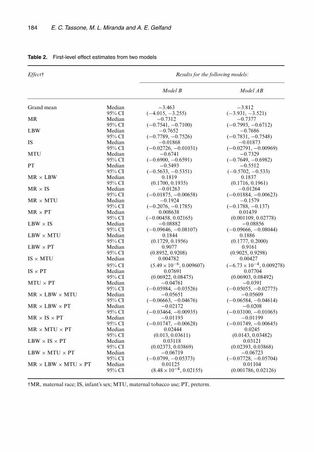
Table 2 provides main effect parameter estimates from the two spatial models (B and AB)and shows the substantial similarity of their results. We note that all main effect parametersobtain statistical significance, on the basis of 95% CIs, in the models. For illustration of ourmethodology, we employ the more parsimonious model B in what follows.

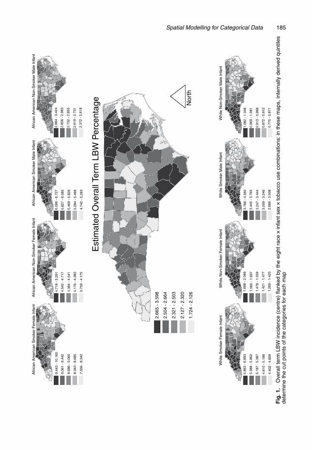
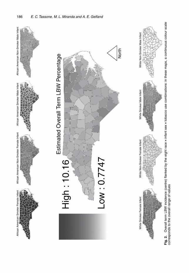
We next turn to other quantities of interest that can be built from the disaggregated proba-bilities. Fig. 1 shows estimated incidence of term LBW in its centre map, flanked by analogousmaps for the eight race× infant sex× tobacco use subgroups. In Fig. 1 internally derived quin-tiles determine the cut points of the categories for each map, so, despite being on very differentscales, the darkest shading denotes, in each map, the 20 counties with highest incidence, per-mitting us to make a particular type of relative comparison. Fig. 2 displays the same estimatesof term LBW incidence, but with ‘global’ quintiles based on the rates over all eight of therace× infant sex× tobacco use subgroups, permitting absolute comparison across maps. Figs 1and 2 together help to illuminate the story. Fig. 1 is most effective for seeing within-map vari-ation whereas Fig. 2 reveals across-map variation. Though the flanking maps in Fig. 2 do notindividually reveal much variation, a comparison between them is striking.

There are several striking features in Figs 1 and 2 that demonstrate the utility of our disag-gregation model. In Fig. 1, the large central map of overall term LBW incidence shows thatcounties in eastern North Carolina generally suffer higher overall incidence. However, the eight

Table 1. Model fit metrics for four models

Metric Results for the following models:

Model 0 Model A Model B Model AB

MSE Median×10−4 261.3 243.6 5.10 5.1495% CI×10−4 (260.9, 261.8) (243.0, 244.1) (4.49, 5.89) (4.52, 5.97)

log.p/ Median 8376 8665 2956 296495% CI (8326, 8429) (8593, 8741) (2867, 3053) (2877, 3062)

χ2 Median 71650 64310 3205 322695% CI (71300, 72010) (63960, 64670) (3092, 3331) (3113, 3351)

KL Median 14.92 14.38 1.098 1.10895% CI (14.89, 14.95) (14.36, 14.41) (1.062, 1.139) (1.072, 1.150)


Table 2. First-level effect estimates from two models

Effect† Results for the following models:

Model B Model AB

Grand mean Median −3.463 −3.81295% CI (−4.015, −3.255) (−3.931, −3.521)

MR Median −0.7312 −0.737795% CI (−0.7541, −0.7100) (−0.7993, −0.6712)

LBW Median −0.7652 −0.768695% CI (−0.7789, −0.7526) (−0.7831, −0.7548)

IS Median −0.01868 −0.0187395% CI (−0.02726, −0.01031) (−0.02791, −0.00969)

MTU Median −0.6741 −0.732995% CI (−0.6900, −0.6591) (−0.7649, −0.6982)

PT Median −0.5493 −0.551295% CI (−0.5633, −0.5351) (−0.5702, −0.533)

MR × LBW Median 0.1819 0.183795% CI (0.1700, 0.1935) (0.1716, 0.1961)

MR × IS Median −0.01263 −0.0126495% CI (−0.01875, −0.00658) (−0.01884, −0.00623)

MR × MTU Median −0.1924 −0.157995% CI (−0.2076, −0.1785) (−0.1788, −0.137)

MR × PT Median 0.008638 0.0143995% CI (−0.00458, 0.02165) (0.001109, 0.02778)

LBW × IS Median −0.08882 −0.0885695% CI (−0.09646, −0.08107) (−0.09666, −0.08044)

LBW × MTU Median 0.1844 0.188695% CI (0.1729, 0.1956) (0.1777, 0.2000)

LBW × PT Median 0.9077 0.916195% CI (0.8952, 0.9208) (0.9025, 0.9298)

IS × MTU Median 0.004782 0.0042795% CI (5:49×10−6, 0.009607) (−6:73×10−4, 0.009278)

IS × PT Median 0.07691 0.0770495% CI (0.06922, 0.08475) (0.06903, 0.08492)

MTU × PT Median −0.04761 −0.039195% CI (−0.05984, −0.03526) (−0.05055, −0.02775)

MR × LBW × MTU Median −0.05651 −0.0560995% CI (−0.06663, −0.04676) (−0.06584, −0.04614)

MR × LBW × PT Median −0.02172 −0.020895% CI (−0.03464, −0.00935) (−0.03100, −0.01065)

MR × IS × PT Median −0.01193 −0.0119995% CI (−0.01747, −0.00628) (−0.01749, −0.00645)

MR × MTU × PT Median 0.02444 0.024595% CI (0.013, 0.03611) (0.0143, 0.03482)

LBW × IS × PT Median 0.03118 0.0312195% CI (0.02373, 0.03869) (0.02393, 0.03868)

LBW × MTU × PT Median −0.06719 −0.0672395% CI (−0.0799, −0.05373) (−0.07728, −0.05704)

MR × LBW × MTU × PT Median 0.01125 0.0110495% CI (8:48×10−4, 0.02155) (0.001786, 0.02126)

†MR, maternal race; IS, infant’s sex; MTU, maternal tobacco use; PT, preterm.

Spatial Modelling for Categorical Data 185A

fric

an A

mer

ican

Sm

oker

Fem

ale

Infa

nt

Whi

te S

mok

er F

emal

e In

fant

Whi

te N

on-S

mok

er F

emal

e In

fant

Whi

te N

on-S

mok

er M

ale

Infa

ntW

hite

Sm

oker

Mal

e In

fant

Nor

th

9.44

3 -

10.1

60

9.06

1 -

9.44

2

8.68

6 -

9.06

0

8.34

3 -

8.68

5

7.55

6 -

8.34

23.

759

- 4.

175

5.86

3 -

6.89

3

5.38

8 -

5.86

2

5.18

7 -

5.38

7

4.81

0 -

5.18

6

4.40

2 -

4.80

91.

269

- 1.

420

2.66

6 -

3.00

8

3.00

9 -

3.24

6

3.24

7 -

3.44

4

3.44

5 -

3.76

5

3.76

6 -

4.56

01.

082

- 1.

346

0.96

9 -

1.08

1

0.91

3 -

0.96

8

0.87

2 -

0.91

2

0.77

5 -

0.87

1

1.42

1 -

1.47

7

1.47

8 -

1.55

9

1.56

0 -

1.69

7

1.69

8 -

2.06

9

2.66

5 -

3.59

8

2.50

4 -

2.66

4

2.32

1 -

2.50

3

2.12

7 -

2.32

0

1.72

4 -

2.12

64.17

6 -

4.38

3

4.38

4 -

4.54

1

4.54

2 -

4.71

7

4.71

8 -

5.29

16.

086

- 6.

727

5.82

7 -

6.08

5

5.46

9 -

5.82

6

5.28

4 -

5.46

8

4.74

2 -

5.28

32.

372

- 2.

618

2.61

9 -

2.73

1

2.73

2 -

2.85

5

2.85

6 -

2.98

3

2.98

4 -

3.42

4

Afr

ican

Am

eric

an N

on-S

mok

er F

emal

e In

fant

Afr

ican

Am

eric

an N

on-S

mok

er M

ale

Infa

ntA

fric

an A

mer

ican

Sm

oker

Mal

e In

fant

Est

imat

ed O

vera

ll Te

rm L

BW

Per

cent

age

Fig

.1.

Ove

rall

term

LBW

inci

denc

e(c

entr

e)fla

nked

byth

eei

ghtr

ace

�inf

ants

ex�t

obac

cous

eco

mbi

natio

ns:i

nth

ese

map

s,in

tern

ally

deriv

edqu

intil

esde

term

ine

the

cutp

oint

sof

the

cate

gorie

sfo

rea

chm

ap

186 E. C. Tassone, M. L. Miranda and A. E. GelfandA

fric

an A

mer

ican

Sm

oker

Fem

ale

Infa

nt

Whi

te S

mok

er F

emal

e In

fant

Whi

te N

on-S

mok

er F

emal

e In

fant

Whi

te N

on-S

mok

er M

ale

Infa

ntW

hite

Sm

oker

Mal

e In

fant

Afr

ican

Am

eric

an N

on-S

mok

er F

emal

e In

fant

Est

imat

ed O

vera

ll Te

rm L

BW

Per

cent

age Nor

th

Hig

h : 1

0.16

Low

: 0.

7747

Afr

ican

Am

eric

an N

on-S

mok

er M

ale

Infa

ntA

fric

an A

mer

ican

Sm

oker

Mal

e In

fant

Fig

.2.

Ove

rall

term

LBW

inci

denc

e(c

entr

e)fla

nked

byth

eei

ght

race

�inf

ants

ex�t

obac

cous

eco

mbi

natio

ns:i

nth

ese

map

s,a

cont

inuo

usco

lour

scal

eco

rres

pond

sto

the

over

allr

ange

ofva

lues


flanking maps of the race× infant sex× tobacco use subgroups tell a different story. Counties innorth-western North Carolina tend to have higher incidence rates for each subgroup. The overallincidence map is subject to confounding with respect to county level composition of the eightsubgroups, i.e., in the overall map, a county’s rate is a weighted average of the eight subgrouprates, but the precise weighting differs from county to county in North Carolina, leading to theSimpson’s paradox situation (Agresti, 2002) that emerges in the ensemble of maps.

The notable visual impression from Fig. 2 is the lack of overlap among the eight flankingsubgroup maps. For example, the counties in the upper leftmost map (for female infants bornto African American mothers who used tobacco during pregnancy) are entirely in the upperquintile, whereas nearly every county in the lower rightmost map (for male infants born to whitemothers who did not use tobacco during pregnancy) belongs to the lowest quintile. In this vein,the centre map in Fig. 2 shows that the variability in overall county term LBW birth incidence israther small compared with the variability across the eight subgroup maps, and that within-mapvariability is small compared with across-map variability.

In addition, Fig. 2 recapitulates the parameter estimates from Table 2, particularly for theinteraction of maternal race and LBW (MR×LBW). Table 2 shows that the magnitude of thiseffect (0.1819 in model B) is similar to the magnitude of the effect for the interaction of LBWand maternal tobacco use (LBW×MTU; 0.1844 in model B). Comparing the range of values in

(a) the leftmost map in the lower row with the map second from the left in the upper row and(b) the map second from the right in the lower row with the rightmost map in the upper row

demonstrates what these parameter estimates also show: the effect of maternal race on LBWincidence is about the same as the effect of maternal tobacco use. Such conclusions might bedifficult to obtain with other modelling approaches.

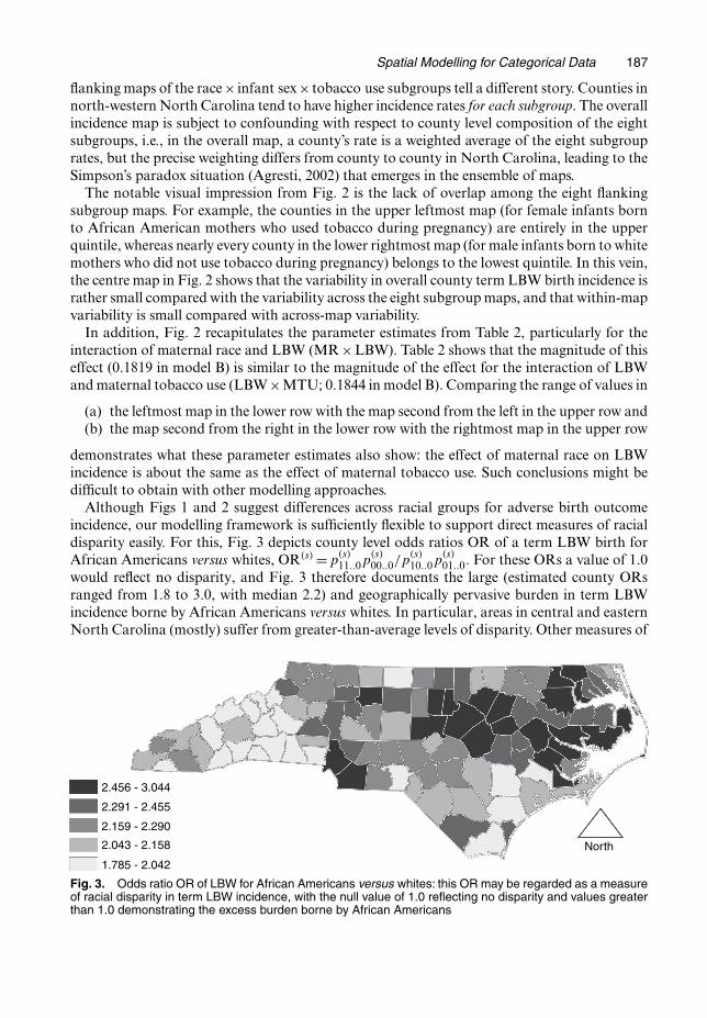
Although Figs 1 and 2 suggest differences across racial groups for adverse birth outcomeincidence, our modelling framework is sufficiently flexible to support direct measures of racialdisparity easily. For this, Fig. 3 depicts county level odds ratios OR of a term LBW birth forAfrican Americans versus whites, OR.s/ =p

.s/11::0p

.s/00::0=p

.s/10::0p

.s/01::0. For these ORs a value of 1.0

would reflect no disparity, and Fig. 3 therefore documents the large (estimated county ORsranged from 1.8 to 3.0, with median 2.2) and geographically pervasive burden in term LBWincidence borne by African Americans versus whites. In particular, areas in central and easternNorth Carolina (mostly) suffer from greater-than-average levels of disparity. Other measures of

2.456 - 3.044

2.291 - 2.455

2.159 - 2.290

2.043 - 2.158

1.785 - 2.042

North

Fig. 3. Odds ratio OR of LBW for African Americans versus whites: this OR may be regarded as a measureof racial disparity in term LBW incidence, with the null value of 1.0 reflecting no disparity and values greaterthan 1.0 demonstrating the excess burden borne by African Americans


disparity, such as those advocated by the Centers for Disease Control and Prevention (Keppelet al., 2005), may also be built from the model output.

By viewing Fig. 3 in conjunction with Fig. 1 and/or Fig. 2, we see that

(a) disparity can be high even where incidence of term LBW is relatively low for both AfricanAmerican and white mothers,

(b) disparity can be low even where term LBW incidence is relatively high for both AfricanAmerican and white mothers and

(c) disparity can (of course) be high where African American mothers have relatively highterm LBW incidence while white mothers have relatively low incidence.

For (a) and (b), policy makers might have competing interests and trade-offs to consider incrafting intervention strategies, whereas for (c) intervention strategies might be focused on asubset of the county population. Such intervention strategies based on Figs 1–3 could considerwhether to target the geographic areas with the worst overall outcomes, the subpopulationswith the worst outcomes, areas with the worst racial disparity or some combination of these.

4.2. Comparing the conditional and disaggregation approachesFinally, we compare our approach with the conditional model given in Section 3.1. We considertwo different outcomes for this comparison:

(a) term LBW, as in Section 4.1, and(b) LBW.

For fits to the North Carolina birth record data, the county level 95% CIs from the conditionalmodel are wider than the corresponding 95% CIs from the disaggregation model for both out-comes. For term LBW, the county level CIs are on average about 30% wider whereas for LBWthe CIs are on average about 25% wider, and in many cases more than 40% wider (for bothoutcomes). Further, for the four largest counties (each with over 20000 births), where we wouldexpect both models to perform well, the CIs are still about 15% wider for the usual model forterm LBW and over 25% wider for LBW. Finally, we recall that, for term LBW, fitting the con-ditional model excluded preterm births from the analysis, whereas the disaggregation approachallows us to use all the data. This may explain the even poorer performance of this model forthis outcome.

To support further the advantages of the disaggregation model, we investigated a simulateddata set. To place the simulation on more familiar terrain for the usual model, we did not includepreterm birth as an outcome, focusing only on the other four dichotomous variables (maternalrace, birth weight outcome, infant sex and maternal tobacco use). Simulated data were gen-erated from a known model similar to the 5 years of North Carolina data and with spatiallyvarying cell probabilities, i.e. cell counts for the 100×24 =1600 categories were generated. Thedisaggregation model was fitted to these cell counts whereas the usual model was fitted to totalsmarginalized over the demographic variables. Model performance was based on estimation ofthe 100 known county level probabilities of LBW. As expected, both models achieved roughly95% empirical coverage: 93/100 for the disaggregation model and 97/100 for the conditionalmodel. However, the CIs were roughly 50% wider for the usual model compared with the disag-gregation model. Also, the disaggregation model had an MSE that was less than half of the MSEfrom the usual model. In other words, the interval estimates for the usual model were too longand not well centred. Lastly, turning to the 100×16=1600 underlying cell probabilities whichthe disaggregation model estimates, satisfyingly, we found 1528 of 1600 CIs (95.5%) containedthe true cell probability.


5. Summary and extensions

We have argued that, in the case where we have observations assigned to areal units but whichretain individual characteristics, there are numerous advantages to modelling at the individuallevel through the use of log-linear models incorporating spatial random effects. In particular, wecan spatially investigate arbitrary marginal and conditional probabilities. In the context of pub-lic health databases, this enables us to illuminate disparities in a richer fashion than previouslyavailable.

In this analysis, we studied term LBW in North Carolina with such a model. We observedpatterns that might have been difficult or impossible to study with other techniques, such asthe higher overall rates in eastern North Carolina yet higher rates for each subgroup in westernNorth Carolina. This same model was used to provide a picture of racial disparity in termLBW, and to classify areas of high disparity into subcategories that might call for differentintervention strategies.

In future work, we shall apply this modelling approach to contingency tables of much higherdimension and to tables involving ordinal classifications. In addition, there will be interest in howselected probabilities and disparities change not only across space but also evolve in time, forinstance, under an annual model for the birth record data from Section 1.2. This will lead us todynamic versions of our approach, perhaps through space–time auto-regressive random-effectsspecifications.

Finally, there are data sets where we do have the geocoded locations that are associated withthe individuals. This would encourage us to work at the point level rather than the areal unitlevel. Conceptually, we would envision a spatial process of log-linear models. Practically, wewould have one multinomial trial at each of n =ΣS

s=1n.s/· locations rather than n multinomial

trials ignoring location or using only areal unit information. Structured spatial dependenceenables us to handle the former case, and investigation of this approach is currently work inprogress.

Acknowledgements

We thank Sharon Edwards for preparing the North Carolina birth record database for analysisand Joshua Tootoo for preparing the maps displaying output from the analysis. We also thankDr Geeta Swamy and Simone Gray for their contributions to the analysis. This publication wasmade possible by grant 5P20-RR-020782-03 from the National Center for Research Resources,a component of the National Institutes of Health, and by grant 5P30-ES-011961-04 from theNational Institute of Environmental Health Sciences, National Institutes of Health. Its contentsare solely the responsibility of the authors and do not necessarily represent the official views ofthe National Institutes of Health.

Appendix A: Model fitting

We build our fully Bayesian model as follows. For prior distributions, we use φ0t ∼ N.0, 1002/ for t =

1, . . . , r;ηtu ∼N.0, 1002/ for t = 1, . . . , r and u= 1, . . . , q, and {φ.1/t , φ.2/

t , . . . , φ.S/t }∼ CAR.τt / for certain t,

as given in Section 1.2. For the t without spatial structure, φ.1/t =φ.2/

t = . . . =φ.S/t = 0, with the exception

of the grand mean term. For the grand mean term, each parameter received an N.0, 1002/ prior. Thehyperpriors for the τts are τt ∼gamma.0:5, 0:005/, which is discussed in Wakefield et al. (2001). The jointposterior is

π.φ0, φ.s/, η, τ |n/∝∏

s

∏

l

π.n.s/l |φ0, φ.s/, η, τ /π.φ0/π.φ.s/|τ /π.τ /π.η/,


writing .φ0, φ.s/, η/ for λ. After simplification, the likelihood term is

∏

s

∏

l

exp{− exp.XTl φ0/ exp.XT

l ηws/ exp.XTl φ.s//}{exp.XT

l φ0/ exp.XTl ηws/ exp.XT

l φ.s//}n.s/l

n.s/l !

The resulting full conditional distributions are as follows:

(a) P.φ0t |·/∝∏

s

∏l exp{n

.s/l XT

l φ0 − exp.XTl φ0/ exp.XT

l ηws/ exp.XTl φ.s//− .φ0

t /2=.2×1002/};

(b) P.φ.s/t |·/∝∏

l exp{n.s/l XT

l φ.s/ −exp.XTl φ0/ exp.XT

l ηws/ exp.XTl φ.s//−τtωs:.φ

.s/t − φ̄

.s/

t /2=2}, where δs

is the set of neighbours of s, defined by adjacency so that ωsv = 1 if v ∈ δs (and otherwise ωsv = 0)with the convention that ωss =0, where ωs: =ΣS

v=1ωsv, and where φ̄.s/

t = .1=ωs:/ΣSv=1ωsvφ

.v/t ;

(c) P.ηtu|·/∝∏s

∏l exp{n

.s/l XT

l ηws − exp.XTl φ0/ exp.XT

l ηws/ exp.XTl φ.s//−η2

tu=.2×1002/};(d) P.τt |·/∼gamma{0:5+S=2, 0:0005+ 1

2 ΣSs=1Σv<sωsv.φ

.s/t −φ.v/

t /2}, based on Mollié (1996).

We implemented our fully Bayesian model by using Markov chain Monte Carlo methods (Gilks et al.,1996). We ran three overdispersed, random, parallel chains of 15000 Markov chain Monte Carlo simula-tions, discarding the first 5000 iterations from each chain as burn-in and retaining every 10th iteration afterburn-in (to reduce potential problems with auto-correlation), for a total of 3×10000=30000 samples forposterior inference. There were no problems with convergence on the basis of Gelman–Rubin statisticsand visual inspection of the mixing of the chains (Gelman and Rubin, 1992).

References

Agresti, A. (2002) Categorical Data Analysis. New York: Wiley.Banerjee, S., Carlin, B. P. and Gelfand, A. E. (2004) Hierarchical Modeling and Analysis for Spatial Data. Boca

Raton: Chapman and Hall–CRC.Besag, J. (1974) Spatial interaction and the statistical analysis of lattice systems (with discussion). J. R. Statist.

Soc. B, 36, 192–236.Besag, J., York, J. and Mollié, A. (1991) Bayesian image restoration, with two applications in spatial statistics.

Ann. Inst. Statist. Math., 43, 1–20.Clayton, D. and Kaldor, J. (1987) Empirical Bayes estimates of age-standardized relative risks for use in disease

mapping. Biometrics, 43, 671–681.Fleiss, J. L., Levin, B. and Paik, M. (2003) Statistical Methods for Rates and Proportions, 3rd edn. New York:

Wiley.Gelfand, A. E. and Vounatsou, P. (2003) Proper multivariate conditional autoregressive models for spatial data

analysis. Biostatistics, 4, 11–15.Gelman, A. and Price, P. N. (1999) All maps of parameter estimates are misleading. Statist. Med., 18, 3221–3234.Gelman, A. and Rubin, D. (1992) Inference from iterative simulation using multiple sequences. Statist. Sci., 7,

457–472.Gilks, W. R., Richardson, S. and Spiegelhalter, D. J. (eds) (1996) Markov Chain Monte Carlo in Practice. London:

Chapman and Hall.Jin, X., Carlin, B. P. and Banerjee, S. (2005) Generalized hierarchical multivariate CAR models for areal data.

Biometrics, 61, 950–961.Keppel, K., Pamuk, E., Lynch, J., Carter-Pokras, O., Kim, I., Mays, V., Pearcy, J., Schoenbach, V. and Weissman,

J. (2005) Methodological issues in measuring health disparities. Vitl Hlth Statist., ser. 2, no. 141.Kullback, S. and Leibler, R. A. (1951) On information and sufficiency. Ann. Math. Statist., 22, 79–86.Mollié, A. (1996) Bayesian mapping of disease. In Markov Chain Monte Carlo in Practice (eds W. R. Gilks, S.

Richardson and D. J. Spiegelhalter), pp. 359–379. London: Chapman and Hall.Raudenbush, S. W. and Bryk, A. S. (2002) Hierarchical Linear Models: Applications and Data Analysis Methods.

Thousand Oaks: Sage.Simpson, E. H. (1951) The interpretation of interaction in contingency tables. J. R. Statist. Soc. B, 13, 238–241.US Department of Health and Human Services (2000) Healthy People 2010: Understanding and Improving Health,

2nd edn. Washington DC: US Government Printing Office.Wakefield, J., Best, N. and Waller, L. (2001) Bayesian approaches to disease mapping. In Spatial Epidemiology:

Methods and Applications (eds P. Elliott, J. Wakefield, N. Best and D. Briggs), pp. 104–127. Oxford: OxfordUniversity Press.

Waller, L. A., Carlin, B. P., Xia, H. and Gelfand, A. E. (1997) Hierarchical spatio-temporal mapping of diseaserates. J. Am. Statist. Ass., 92, 607–617.

Waller, L. and Gotway, C. (2004) Applied Spatial Statistics for Public Health Data. New York: Wiley.

Disaggregated spatial modelling for areal unit categorical data

Documents

Transcript of Disaggregated spatial modelling for areal unit categorical data