DISC: Data-Intensive Similarity Measure for Categorical Data

DISC: Data-Intensive Similarity Measure forCategorical Data

Aditya Desai, Himanshu Singh and Vikram Pudi

International Institute of Information Technology-Hyderabad,Hyderabad, India

{aditya.desai,himanshu.singh}@research.iiit.ac.in,[email protected]

http://iiit.ac.in

Abstract. The concept of similarity is fundamentally important in al-most every scientific field. Clustering, distance-based outlier detection,classification, regression and search are major data mining techniqueswhich compute the similarities between instances and hence the choiceof a particular similarity measure can turn out to be a major cause ofsuccess or failure of the algorithm. The notion of similarity or distancefor categorical data is not as straightforward as for continuous data andhence, is a major challenge. This is due to the fact that different valuestaken by a categorical attribute are not inherently ordered and hence anotion of direct comparison between two categorical values is not pos-sible. In addition, the notion of similarity can differ depending on theparticular domain, dataset, or task at hand. In this paper we present anew similarity measure for categorical data DISC - Data-Intensive Simi-larity Measure for Categorical Data. DISC captures the semantics of thedata without any help from domain expert for defining the similarity. Inaddition to these, it is generic and simple to implement. These desirablefeatures make it a very attractive alternative to existing approaches. Ourexperimental study compares it with 14 other similarity measures on 24standard real datasets, out of which 12 are used for classification and 12for regression, and shows that it is more accurate than all its competitors.

Keywords: Categorical similarity measures, cosine similarity, knowl-edge discovery, classification, regression

1 IntroductionThe concept of similarity is fundamentally important in almost every scientificfield. Clustering, distance-based outlier detection, classification and regressionare major data mining techniques which compute the similarities between in-stances and hence choice of a particular similarity measure can turn out to be amajor cause of success or failure of the algorithm. For these tasks, the choice ofa similarity measure can be as important as the choice of data representation orfeature selection. Most algorithms typically treat the similarity computation asan orthogonal step and can make use of any measure. Similarity measures canbe broadly divided in two categories: similarity measures for continuous dataand categorical data.

The notion of similarity measure for continuous data is straightforward dueto inherent numerical ordering. Minkowski distance and its special case, the

2 Aditya Desai, Himanshu Singh, Vikram Pudi

Euclidean distance are the two most widely used distance measures for contin-uous data. However, the notion of similarity or distance for categorical data isnot as straightforward as for continuous data and hence is a major challenge.This is due to the fact that the different values that a categorical attribute takesare not inherently ordered and hence a notion of direct comparison between twocategorical values is not possible. In addition, the notion of similarity can differdepending on the particular domain, dataset, or task at hand.

Although there is no inherent ordering in categorical data, there are otherfactors like co-occurrence statistics that can be effectively used to define whatshould be considered more similar and vice-versa. This observation has motivatedresearchers to come up with data-driven similarity measures for categorical at-tributes. Such measures take into account the frequency distribution of differentattribute values in a given data set but most of these algorithms fail to captureany other feature in the dataset apart from frequency distribution of differentattribute values in a given data set. One solution to the problem is to build acommon repository of similarity measures for all commonly occurring concepts.As an example, let the similarity values for the concept “color” be determined.Now, consider 3 colors red, pink and black. Consider the two domains as follows:

– Domain I: The domain is say determining the response of cones of the eyeto the color, then it is obvious that the cones behave largely similarly to redand pink as compared to black. Hence similarity between red and pink mustbe high compared to the similarity between red and black or pink and black.

– Domain II: Consider another domain, for example the car sales data. Insuch a domain, it may be known that the pink cars are extremely rare ascompared to red and black cars and hence the similarity between red andblack must be larger than that between red and pink or black and pink inthis case.

Thus, the notion of similarity varies from one domain to another and hence theassignment of similarity must involve a thorough understanding of the domain.Ideally, the similarity notion is defined by a domain expert who understands thedomain concepts well. However, in many applications domain expertise is notavailable and the users don’t understand the interconnections between objectswell enough to formulate exact definitions of similarity or distance.

In the absence of domain expertise it is conceptually very hard to come upwith a domain independent solution for similarity. This makes it necessary todefine a similarity measure based on latent knowledge available from data insteadof a fit-to-all measure and is the major motivation for this paper.

In this paper we present a new similarity measure for categorical data, DISC– Data-Intensive Similarity Measure for Categorical Data. DISC captures thesemantics of the data without any help from domain experts for defining sim-ilarity. It achieves this by capturing the relationships that are inherent in thedata itself, thus making the similarity measure “data-intensive”. In addition, itis generic and simple to implement.

The remainder of the paper is organized as follows. In Section 2 we discussrelated work and problem formulation in Section 3. We present the DISC algo-

DISC: Data-Intensive Similarity Measure for Categorical Data 3

rithm in Section 4 followed by experimental evaluation and results in Section 5.Finally, in Section 6, we summarize the conclusions of our study and identifyfuture work.

1.1 Key Contributions

– Introducing a notion of similarity between two values of a categorical at-tribute based on co-occurrence statistics.

– Defining a valid similarity measure for capturing such a notion which can beused out-of-the-box for any generic domain.

– Experimentally validating that such a similarity measure provides a signifi-cant improvement in accuracy when applied to classification and regressionon a wide array of dataset domains. The experimental validation is especiallysignificant since it demonstrates a reasonably large improvement in accuracyby changing only the similarity measure while keeping the algorithm and itsparameters constant.

2 Related Work

Determining similarity measures for categorical data is a much studied field asthere is no explicit notion of ordering among categorical values. Sneath andSokal were among the first to put together and discuss many of the categoricalsimilarity measures and discuss this in detail in their book [2] on numericaltaxonomy.

The specific problem of clustering categorical data has been actively stud-ied. There are several books [3–5] on cluster analysis that discuss the problemof determining similarity between categorical attributes. The problem has alsobeen studied recently in [17, 18]. However, most of these approaches do not offersolutions to the problem discussed in this paper, and the usual recommenda-tion is to “binarize” the data and then use similarity measures designed forbinary attributes. Most work has been carried out on development of clusteringalgorithms and not similarity functions. Hence these works are only marginallyor peripherally related to our work. Wilson and Martinez [6] performed a de-tailed study of heterogeneous distance functions (for categorical and continuousattributes) for instance based learning. The measures in their study are basedupon a supervised approach where each data instance has class information inaddition to a set of categorical/continuous attributes.

There have been a number of new data mining techniques for categoricaldata that have been proposed recently. Some of them use notions of similaritywhich are neighborhood-based [7–9], or incorporate the similarity computationinto the learning algorithm[10, 11]. These measures are useful to compute theneighborhood of a point and neighborhood-based measures but not for calcu-lating similarity between a pair of data instances. In the area of informationretrieval, Jones et al. [12] and Noreault et. al [13] have studied several similaritymeasures. Another comparative empirical evaluation for determining similaritybetween fuzzy sets was performed by Zwick et al. [14], followed by several oth-ers [15, 16].


In our experiments we have compared our approach with the methods dis-cussed in [1]; which provides a recent exhaustive comparison of similarity mea-sure for categorical data.

3 Problem Formulation

In this section we discuss the necessary conditions for a valid similarity measure.Later, in Section 4.5 we describe how DISC satisfies these requirements andprove the validity of our algorithm. The following conditions need to hold for adistance metric “d” to be valid where d(x, y) is the distance between x and y.

1. d(x, y) ≥ 02. d(x, y) = 0 if and only if x=y3. d(x, y) = d(y, x)4. d(x, z) ≤ d(x, y) + d(y, z)

In order to come up with conditions for a valid similarity measure we use sim =1

1+dist , a distance-similarity mapping used in [1]. Based on this mapping we comeup with the following definitions for valid similarity measures:

1. 0 ≤ Sim(x, y) ≤ 12. Sim(x, y) = 1 if and only if x = y3. Sim(x, y) = Sim(y, x)4. 1

Sim(x,y) + 1Sim(y,z) ≥ 1 + 1

Sim(x,z)

Where, Sim(x, y) is the similarity between x and y:

4 DISC Algorithm

In this section we present the DISC algorithm. First in Section 4.1 we presentthe motivation for our algorithm followed by data-structure description in Sec-tion 4.2 and a brief overview of the algorithm in Section 4.3. We then describe thealgorithm for similarity matrix computation in Section 4.4. Finally in Section 4.5we validate our similarity measure.

4.1 Motivation and DesignAs can be seen from the related work, current similarity (distance) measuresfor categorical data only examine the number of distinct categories and theircounts without looking at co-occurrence statistics with other dimensions in thedata. Thus, there is a high possibility that, the latent information that comesalong is lost during the process of assigning similarities. Consider the examplein Table 1, let there be a 3-column dataset where the Brand of a car and Colorare independent variables and the Price of the car is a dependant variable. Nowthere are three brands a, b, c with average price 49.33, 32.33, 45.66. It can beintuitively said that based on the available information that similarity betweena and c is greater than that between the categories a and b. This is true inreal life where a, c, b may represent low, medium and high end cars and hencethe similarity between a low-end and a medium-end car will be more than thesimilarity between a low-end and a high-end car. Now the other independentvariable is Color. The average prices corresponding to the three colors namely


Brand Color Price

a red 50

a green 48

a blue 50

b red 32

b green 30

b blue 35

c red 47

c green 45

c blue 45

Table 1. Illustration

red, green and blue are 43, 41, 43.33. As can be seen, there is a small differencein their prices which is in line with the fact that the cost of the car is very looselyrelated to its color.

It is important to note that a notion of similarity for categorical variableshas a cognitive component to it and as such each one is debatable. However,the above explained notion of similarity is the one that best exploits the la-tent information for assigning similarity and will hence give predictors of highaccuracy. This claim is validated by the experimental results. Extracting theseunderlying semantics by studying co-occurrence data forms the motivation forthe algorithm presented in this section.

4.2 Data Structure Description

We first construct a data structure called the categorical information table (CI).The function of the CI table is to provide a quick-lookup for information relatedto the co-occurrence statistics. Thus, for the above example CI[Brand:a][Color:red]= 1, as for only a single instance, Brand:a co-occurs with Color:red. For acategorical-numeric pair, e.g. CI[Brand:a][Price] = 49.33 the value is the meanvalue of the attribute Price for instances whose value for Brand is a.

Now, for every value v of each categorical attribute Ak a representative pointτ(Ak : v) is defined. The representative point is a vector consisting of the meansof all attributes other than Ak for instances where attribute Ak takes value v:

τ(Ak : v) =< µ(Ak : v,A1), . . . , µ(Ak : v,Ad) > (1)

It may be noted that the term µ(Ak : v,Ak) is skipped in the above expression.As there is no standard notion of mean for categorical attributes we define it as

µ(Ak : v,Ai) =< CI[Ak : v][Ai : vi1], . . . , CI[Ak : v][Ai : vin] > (2)where domain(Ai) = {vi1, . . . , vin} It can thus be seen that, the mean itself is apoint in a n-dimensional space having dimensions as vi1,. . . ,vin with magnitudes:< CI[Ak : v][Ai : vi1], . . . , CI[Ak : v][Ai : vin] >.Initially all distinct values belonging to the same attribute are conceptuallyvectors perpendicular to each other and hence the similarity between them is 0.

For, the given example, the mean for dimension Color when Brand : a isdenoted as µ(Brand : a,Color). As defined above, the mean in a categorical


dimension is itself a point in a n-dimensional space and hence, the dimensionsof mean for the attribute Color are red, blue, green and henceµ(Brand : a,Color) = {CI[Brand : a][Color : red], CI[Brand : a][Color :blue], CI[Brand : a][Color : green]}Similarly, µ(Brand : a, Price) = {CI[Brand : a][Price]}

Thus the representative point for the value a of attribute Brand is given by,τ(Brand : a) =< µ(Brand : a,Color), µ(Brand : a, Price) >

4.3 Algorithm Overview

Initially we calculate the representative points for all values of all attributes. Wethen initialize similarity in a manner similar to the overlap similarity measurewhere matches are assigned similarity value 1 and the mismatches are assignedsimilarity value 0. Using the representative points calculated above, we assign anew similarity between each pair of values v, v′ belonging to the same attributeAk as equal to the average of cosine similarity between their means for eachdimension. Now the cosine similarity between v and v′ in dimension Ai is denotedby CS(v : v′, Ai) and is equal to the cosine similarity between vectors µ(Ak :v,Ai) and µ(Ak : v′, Ai). Thus, similarity between Ak : v and Ak : v′ is:∑d

l=0,l 6=i CS(v : v′, Al)

d− 1Thus, for the above example, the similarity between Brand:a and Brand:b is theaverage of cosine similarity between their respective means in dimensions Color

and Price. Thus Sim(a, b) is given as: CS(a:b,Color)+CS(a:b,Price)2

An iteration is said to have been completed, when similarity between allpairs of values belonging to the same attribute (for all attributes) are computedusing the above methodology. These, new values are used for cosine similaritycomputation in the next iteration.

4.4 DISC ComputationIn this section, we describe the DISC algorithm and hence the similarity ma-trix construction. The similarity matrix construction using DISC is described asfollows:

1. The similarity matrix is initialized in a manner similar to overlap similaritymeasure where ∀i,j,kSim(vij , vik) = 1, if vij = vik and Sim(vij , vik) = 0,if vij 6= vik

2. Consider a training dataset to be consisting of n tuples. The value of thefeature variable Aj corresponding to the ith tuple is given as Trainij . Weconstruct a data-structure “Categorical Information” which for any categor-ical value (vil) of attribute Ai returns number of co-occurrences of value vjktaken by feature variable Aj if Aj is categorical and returns the mean valueof feature variable Aj for the corresponding set of instances if it is numeric.Let this data-structure be denoted by CI. The value corresponding to thenumber of co-occurrences of categorical value vjk when feature variable Ai

takes value vil is given by CI[Ai, vil][Aj , vjk] when Aj is categorical. Also,when Aj is numeric, CI[Ai, vil][Aj ] corresponds to the mean of values takenby attribute Aj when Ai takes value vil.


3. The Sim(vij ,vik) (Similarity between categorical values vij and vik) is nowcalculated as the average of the per-attribute cosine similarity between theirmeans (Similaritym), where the means have a form as described above.The complicated nature of cosine product arises due to the fact that, thetransformed space after the first iteration has dimensions which are no longerorthogonal (i.e. Sim(vij , vik) is no longer 0).

Similaritym =

{1− |CI[Ai:vij ][Am]−CI[Ai:vik][Am]|

Max[Am]−Min[Am]; ifAm is Numeric

CS(µ(Ai : vij , Am), µ(Ai : vik, Am)); ifAm is Categorical

where CS(µ(Ai : vij , Am), µ(Ai : vik, Am)) is defined as follows :∑vml,vml̄εAm

CI[Ai : vij ][Am : vml] ∗ CI[Ai : vik][Am : Vml̄] ∗ Sim(vml̄, vml)

NormalV ector1 ∗NormalV ector2

NormalV ector1 = (∑vml,vml̄εAm

CI[Ai : vij ][Am : vml] ∗ CI[Ai : vij ][Am, vml̄] ∗ Sim(vml, vml̄))1/2

NormalV ector2 = (∑vml,vml̄εAm

CI[Ai : vik][Am : vml] ∗ CI[Ai : vik][Am, vml̄] ∗ Sim(vml, vml̄))1/2

Sim(vij , vik) = 1d−1

∑dm=1,m 6=i Similaritym

Table 2. Cosine Similarity computation between vij , vik

4. The matrix is populated using the above equation for all combinations∀i,j,kSim(vij , vik). To test the effectiveness of the similarity matrix, we plugthe similarity values in a classifier (the nearest neighbour classifier in ourcase) in case of classification and compute its accuracy on a validation set.If the problem domain is regression we plug in the similarity values into aregressor (the nearest neighbour regressor in our case) and compute the cor-responding root mean square error. Thus, such an execution of 3 followed by4 is termed an iteration.

5. The step 3 is iterated on again using the new similarity values until theaccuracy parameter stops increasing. The matrix obtained at this iterationis the final similarity matrix that is used for testing. (In case of regressionwe stop when the root mean square error increases.)

In addition, the authors have observed that, most of the improvement takesplace in the first iteration and hence in domains like clustering (unsuper-vised) or in domains with tight limits on training time the algorithm can behalted after the first iteration.

4.5 Validity of Similarity Measure

The similarity measure proposed in this paper is basically a mean of cosine simi-larities derived for individual dimensions in non-orthogonal spaces. The validityof the similarity measure can now be argued as follows:


1. As the similarity measure is a mean of cosine similarities which have a rangefrom 0-1, it is implied that the range of values output by the similaritymeasure will be between 0-1 thus satisfying the first constraint.

2. For the proposed similarity measure Sim(X,Y ) = 1, if and only if Simk(Xk, Yk) =1 for all feature variables Ak. Now, constraint 2 will be violated if X 6= Y andSim(X,Y ) = 1. This implies that there exists an Xk, Yk such that Xk 6= Ykand for which Sim(Xk, Yk) = 1. Now for Sim(Xk, Yk) = 1 implies cosineproduct of CI[Ak : Xk][Am] and CI[Ak : Yk][Am] is 1 for all Am whichimplies that CI[Ak : Xk][Am], CI[Ak : Yk][Am] are parallel and hence canbe considered to be equivalent with respect to the training data.

3. As cosine product is commutative, the third property holds implicitly.4. It may be noted that the resultant similarity is a mean of similarities com-

puted for each dimension. Also, the similarity for each dimension is in essencea cosine product and hence, the triangle inequality holds for each componentof the sum. Thus the fourth property is satisfied.

5 Experimental Study

In this section, we describe the pre-processing steps and the datasets used inSection 5.1 followed by experimental results in Section 5.2. Finally in Section 5.3we provide a discussion on the experimental results.

5.1 Pre-Processing and Experimental Settings

For our experiments we used 24 datasets out of which 12 were used for classi-fication and 12 for regression. We compare our approach with the approachesdiscussed in [1], which provides a recent exhaustive comparison of similaritymeasures for categorical data.

Eleven of the datasets used for classification were purely categorical and onewas numeric (Iris). Different methods can be used to handle numeric attributesin datasets like discretizing the numeric variables using the concept of minimumdescription length [20] or equi-width binning. Another possible way to handle amixture of attributes is to compute the similarity for continuous and categoricalattributes separately, and then do a weighted aggregation. For our experimentswe used MDL for discretizing numeric variables for classification datasets.

Nine of the datasets used for regression were purely numeric, two (Abaloneand Auto Mpg) were mixed while one (Servo) was purely categorical. It maybe noted that the datasets used for regression were discretized using equi-widthbinning using the following weka setting: “weka.filters.unsupervised.attribute.Discretize−B10−M − 1.0−Rfirst− last” The k-Nearest Neighbours (kNN)was implemented with number of neighbours 10. The weight associated witheach neighbour was the similarity between the neighbour and the input tuple.The class with the highest weighted votes was the output class for classificationwhile the output for regression was a weighted sum of the individual responses.

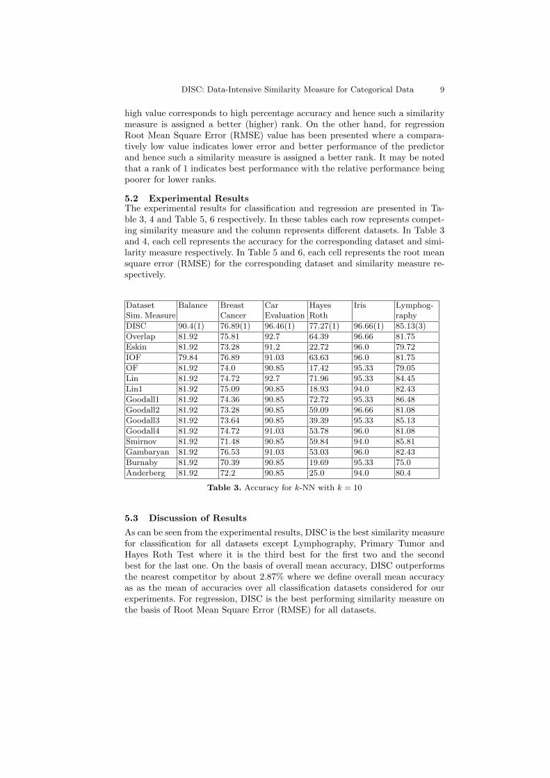
The results have been presented for 10-folds cross-validation. Also, for ourexperiments we used the entire train set as the validation set. The numbers inbrackets indicate the rank of DISC versus all other competing similarity mea-sures. For classification, the values indicate the accuracy of the classifier where a


high value corresponds to high percentage accuracy and hence such a similaritymeasure is assigned a better (higher) rank. On the other hand, for regressionRoot Mean Square Error (RMSE) value has been presented where a compara-tively low value indicates lower error and better performance of the predictorand hence such a similarity measure is assigned a better rank. It may be notedthat a rank of 1 indicates best performance with the relative performance beingpoorer for lower ranks.

5.2 Experimental ResultsThe experimental results for classification and regression are presented in Ta-ble 3, 4 and Table 5, 6 respectively. In these tables each row represents compet-ing similarity measure and the column represents different datasets. In Table 3and 4, each cell represents the accuracy for the corresponding dataset and simi-larity measure respectively. In Table 5 and 6, each cell represents the root meansquare error (RMSE) for the corresponding dataset and similarity measure re-spectively.

DatasetSim. Measure

Balance BreastCancer

CarEvaluation

HayesRoth

Iris Lymphog-raphy

DISC 90.4(1) 76.89(1) 96.46(1) 77.27(1) 96.66(1) 85.13(3)

Overlap 81.92 75.81 92.7 64.39 96.66 81.75

Eskin 81.92 73.28 91.2 22.72 96.0 79.72

IOF 79.84 76.89 91.03 63.63 96.0 81.75

OF 81.92 74.0 90.85 17.42 95.33 79.05

Lin 81.92 74.72 92.7 71.96 95.33 84.45

Lin1 81.92 75.09 90.85 18.93 94.0 82.43

Goodall1 81.92 74.36 90.85 72.72 95.33 86.48

Goodall2 81.92 73.28 90.85 59.09 96.66 81.08

Goodall3 81.92 73.64 90.85 39.39 95.33 85.13

Goodall4 81.92 74.72 91.03 53.78 96.0 81.08

Smirnov 81.92 71.48 90.85 59.84 94.0 85.81

Gambaryan 81.92 76.53 91.03 53.03 96.0 82.43

Burnaby 81.92 70.39 90.85 19.69 95.33 75.0

Anderberg 81.92 72.2 90.85 25.0 94.0 80.4

Table 3. Accuracy for k-NN with k = 10

5.3 Discussion of Results

As can be seen from the experimental results, DISC is the best similarity measurefor classification for all datasets except Lymphography, Primary Tumor andHayes Roth Test where it is the third best for the first two and the secondbest for the last one. On the basis of overall mean accuracy, DISC outperformsthe nearest competitor by about 2.87% where we define overall mean accuracyas as the mean of accuracies over all classification datasets considered for ourexperiments. For regression, DISC is the best performing similarity measure onthe basis of Root Mean Square Error (RMSE) for all datasets.


DatasetSim. Measure

PrimaryTumor

HayesRothTest

TicTacToe

Zoo TeachingAssist.

Nursery MeanAccuracy

DISC 41.66(3) 89.28(2) 100.0(1) 91.08(1) 58.94(1) 98.41(1) 83.51(1)

Overlap 41.66 82.14 92.48 91.08 50.33 94.75 78.81

Eskin 41.36 75.0 94.46 90.09 50.33 94.16 74.19

IOF 38.98 71.42 100.0 90.09 47.01 94.16 77.57

OF 40.17 60.71 84.96 89.1 43.7 95.74 71.08

Lin 41.66 67.85 95.82 90.09 56.95 96.04 79.13

Lin1 42.26 42.85 82.56 91.08 54.96 93.54 70.87

Goodall1 43.15 89.28 97.07 89.1 51.65 95.74 80.64

Goodall2 38.09 92.85 91.54 88.11 52.98 95.74 78.52

Goodall3 41.66 71.42 95.51 89.1 50.99 95.74 75.89

Goodall4 32.73 82.14 96.24 89.1 55.62 94.16 77.38

Smirnov 42.55 78.57 98.74 89.1 54.3 95.67 78.57

Gambaryan 39.58 89.28 98.74 90.09 50.33 94.16 78.59

Burnaby 3.86 60.71 83.29 71.28 40.39 90.85 65.30

Anderberg 37.79 53.57 89.14 90.09 50.33 95.74 71.75

Table 4. Accuracy for k-NN with k = 10

Dataset Comp.Strength

Flow Abalone Bodyfat Housing Whitewine

DISC 4.82(1) 13.2(1) 2.4(1) 0.6(1) 4.68(1) 0.74(1)

Overlap 6.3 15.16 2.44 0.65 5.4 0.74

Eskin 6.58 16.0 2.45 0.66 6.0 0.77

IOF 6.18 15.53 2.42 0.76 5.48 0.75

OF 6.62 14.93 2.41 0.66 5.27 0.75

Lin 6.03 16.12 2.4 0.63 5.3 0.74

Lin1 7.3 16.52 2.41 0.87 5.41 0.74

Goodall1 6.66 14.97 2.41 0.64 5.27 0.74

Goodall2 6.37 15.09 2.43 0.66 5.33 0.75

Goodall3 6.71 14.96 2.41 0.65 5.27 0.74

Goodall4 5.98 15.67 2.47 0.71 6.4 0.78

Smirnov 6.89 15.5 2.4 0.67 5.17 0.74

Gambaryan 6.01 15.46 2.46 0.67 5.73 0.76

Burnaby 6.63 15.23 2.41 0.65 5.32 0.74

Anderberg 7.15 15.16 2.42 0.67 5.84 0.75

Table 5. RMSE for k-NN with k = 10

For classification datasets like Iris, Primary Tumor and Zoo the algorithmhalted after the 1st iteration while for datasets like Balance, Lymphography,Tic-Tac-Toe, Breast Cancer the algorithm halted after the 2nd iteration. Also,for Car-Evaluation, Hayes Roth, Teaching Assistant and Nursery the algorithmhalted after the 3rd iteration while it halted after the 4th iteration for Hayes RothTest. For regression, the number of iterations was less than 5 for all datasets ex-cept Compressive Strength for which it was 9. Thus, it can be seen that thenumber of iterations for all datasets is small. Also, the authors observed thatthe major bulk of the accuracy improvement is achieved with the first iteration


Dataset Slump Servo Redwine Forest Fires Concrete Auto Mpg

DISC 6.79(1) 0.54(1) 0.65(1) 65.96(1) 10.29(1) 2.96(1)

Overlap 7.9 0.78 0.67 67.13 11.61 3.58

Eskin 8.12 0.77 0.68 67.49 11.15 3.98

IOF 8.11 0.77 0.68 67.95 11.36 3.71

OF 7.72 0.8 0.68 67.76 12.55 3.3

Lin 8.33 0.76 0.67 67.16 10.99 3.74

Lin1 8.42 1.1 0.68 67.96 12.16 3.89

Goodall1 7.76 0.77 0.66 67.97 11.45 3.5

Goodall2 7.82 0.81 0.67 68.64 12.21 3.39

Goodall3 7.75 0.78 0.67 68.48 11.52 3.39

Goodall4 7.87 0.95 0.71 70.28 12.96 3.92

Smirnov 8.22 0.78 0.69 67.07 11.59 3.39

Gambaryan 7.8 0.83 0.69 69.54 12.38 3.75

Burnaby 7.89 0.8 0.68 67.73 12.62 3.28

Anderberg 7.94 0.9 0.7 66.63 12.66 3.53

Table 6. RMSE for k-NN with k = 10

and hence for domains with time constraints in training the algorithm can behalted after the first iteration. The reason for the consistently good performancecan be attributed to the fact that a similarity computation is a major componentin nearest neighbour classification and regression techniques, and DISC capturessimilarity accurately and efficiently in a data driven manner.

The computational complexity for determining the similarity measure isequivalent to the computational complexity of computing cosine similarity foreach pair of values belonging to the same categorical attribute. Let the numberof pairs of values, the number of tuples, number of attributes and the averagenumber of values per attribute be V , n, d and v respectively. It can be seen that,construction of categorical collection is O(nd). Also, for all pairs of values V,we compute the similarity as the mean of cosine similarity of their representa-tive points for each dimension. This is essentially (v2d) for each pair and hencethe computationally complexity is O(V v2d) and hence the overall complexityis O(nd + V v2d). Once, the similarity values are computed, using them in anyclassification, regression or a clustering task is a simple table look up and ishence O(1).

6 Conclusion

In this paper we have presented and evaluated DISC, a similarity measure forcategorical data. DISC is data intensive, generic and simple to implement. Inaddition to these features, it doesn’t require any domain expert’s knowledge.Finally our algorithm was evaluated against 14 competing algorithms on 24standard real-life datasets, out of which 12 were used for classification and 12 forregression. It outperformed all competing algorithms on almost all datasets. Theexperimental results are especially significant since it demonstrates a reasonablylarge improvement in accuracy by changing only the similarity measure whilekeeping the algorithm and its parameters constant.


Apart from classification and regression, similarity computation is a pivotalstep in a number of application such as clustering, distance-based outliers detec-tion and search. Future work includes applying our algorithm for these techniquesalso. We also intend to develop a weighing measure for different dimensions forcalculating similarity which will make the algorithm more robust.

References1. Shyam Boriah, Varun Chandola and Vipin Kumar. Similarity Measures for Cate-

gorical Data: A Comparative Evaluation. Proceedings of SDM ’08, Atlanta,Georgia,USA. SIAM, 2008.

2. P. H. A. Sneath and R. R. Sokal. Numerical Taxonomy: The Principles and Practiceof Numerical Classification. W. H. Freeman and Company, San Francisco, 1973.

3. M. R. Anderberg. Cluster Analysis for Applications. Academic Press, 1973.4. A. K. Jain and R. C. Dubes. Algorithms for Clustering Data. Prentice-Hall, Engle-

wood Cliffs NJ, 1988.5. J. A. Hartigan. Clustering Algorithms. John Wiley & Sons, New York, NY, 1975.6. D. R. Wilson and T. R. Martinez. Improved heterogeneous distance functions. J.

Artif. Intell. Res. (JAIR), 6:1–34, 1997.7. Y. Biberman. A context similarity measure. In ECML ’94, pages 49–63.

Springer,1994.8. G. Das and H. Mannila. Context-based similarity measures for categorical databases.

In PKDD ’00, London, UK, 2000. Springer-Verlag.9. C. R. Palmer and C. Faloutsos. Electricity based external similarity of categorical

attributes. In PAKDD ’03 pages 486–500. Springer, 2003.10. Z. Huang. Extensions to the k-means algorithm for clustering large data sets with

categorical values. Data Mining and Knowledge Discovery, 2(3):283–304, 1998.11. V. Ganti, J. Gehrke, and R. Ramakrishnan. CACTUS–clustering categorical data

using summaries. In KDD ’99, New York, NY, USA, 1999. ACM Press12. W. P. Jones and G. W. Furnas. Pictures of relevance: a geometric analysis of

similarity measures. J. Am. Soc. Inf. Sci., 38(6):420–442, 1987.13. T. Noreault, M. McGill, and M. B. Koll. A performance evaluation of similarity

measures, document term weighting schemes and representations in a boolean envi-ronment. In SIGIR ’80: Proceedings of the 3rd annual ACM conference on Researchand development in information retrieval, pages 57–76, Kent, UK, 1981. Butter-worth & Co.

14. R. Zwick, E. Carlstein, and D. V. Budescu. Measures of similarity among fuzzyconcepts: A comparative analysis. International Journal of Approximate Reasoning,1(2):221–242, 1987.

15. C. P. Pappis and N. I. Karacapilidis. A comparative assessment of measures ofsimilarity of fuzzy values. Fuzzy Sets and Systems, 56(2):171–174, 1993.

16. X. Wang, B. De Baets, and E. Kerre. A comparative study of similarity measures.Fuzzy Sets and Systems, 73(2):259–268, 1995.

17. D. Gibson, J. M. Kleinberg, and P. Raghavan. Clustering categorical data: Anapproach based on dynamical systems. VLDB Journal, 8(34):222–236, 2000.

18. S. Guha, R. Rastogi, and K. Shim. ROCK–a robust clusering algorith for categori-cal attributes. In Proceedings of IEEE International Conference on Data Engineer-ing, 1999.

19. I. H. Witten and E. Frank. Data Mining: Practical machine learning tools andtechniques. Morgan Kaufmann, 2 edition, 2005.

20. U. M. Fayyad and K. B. Irani.On the handling of continuous-valued attributes indecision tree generation. Machine Learning, 8:87–102, 1992.

DISC: Data-Intensive Similarity Measure for Categorical Data

Documents

Transcript of DISC: Data-Intensive Similarity Measure for Categorical Data