A new GLM framework for analysing categorical data ...
151
D´ elivr´ e par l’Universit´ e Montpellier II Pr´ epar´ ee au sein de l’´ ecole doctorale I2S * Et des unit´ es de recherche UMR 5149, UMR AGAP Sp´ ecialit´ e: Biostatistique Pr´ esent´ ee par Jean PEYHARDI A new GLM framework for analysing categorical data. Application to plant structure and development. Composition du jury : M. Christophe Biernacki Universit´ e Lille 1 Rapporteur M. Gerhard Tutz Universit´ e Munich Rapporteur Mme H´ el` ene Jacqmin Gadda INSERM Bordeaux Examinatrice M. Christian Lavergne Universit´ e Montpellier 3 Pr´ esident M. Yann Gu´ edon CIRAD Montpellier Directeur de th` ese Mme Catherine Trottier Universit´ e Montpellier 3 Co-directrice de th` ese M. Pierre- ´ Eric Lauri INRA Montpellier Membre invit´ e * I2S: ´ Ecole doctorale Information Structures Syst` emes
-
Upload
khangminh22 -
Category
Documents
-
view
0 -
download
0
Transcript of A new GLM framework for analysing categorical data ...
Delivre par l’Universite Montpellier II
Preparee au sein de l’ecole doctorale I2S∗
Et des unites de recherche UMR 5149, UMR AGAP
Specialite: Biostatistique
Presentee par Jean PEYHARDI
A new GLM framework
for analysing categorical data.
Application to plant structure and development.
Composition du jury :
M. Christophe Biernacki Universite Lille 1 Rapporteur
M. Gerhard Tutz Universite Munich Rapporteur
Mme Helene Jacqmin Gadda INSERM Bordeaux Examinatrice
M. Christian Lavergne Universite Montpellier 3 President
M. Yann Guedon CIRAD Montpellier Directeur de these
Mme Catherine Trottier Universite Montpellier 3 Co-directrice de these
M. Pierre-Eric Lauri INRA Montpellier Membre invite
∗ I2S: Ecole doctorale Information Structures Systemes


A la memoire de Damien, un papillon si vite envole . . .


Acknowledgements
Au dela d’un travail de recherche de trois ans, cette these represente une periode de transition,cloturant mes annees d’etudes et m’ouvrant les portes du monde de la recherche . . . d’emploi !Je passe donc d’une adolescence prolongee a l’age adulte, accompagne durant ce periple pardes sages autant que de grands enfants; je tiens ici a les remercier.
Tout d’abord, je tiens a remercier mes directeurs Yann Guedon et Catherine Trottier, pourm’avoir encadre durant ces trois annees. Je vous remercie pour la confiance que vous m’avezaccordee, laissant de cote certaines attentes presentes dans le sujet initial de these : je devaispasser trois mois sur ces modeles pour donnees categorielles, j’y ai finalement passe trois ans !
Yann, tu as su lire entre les lignes de mon CV, qui reflete un parcours quelque peu tu-multueux, et me donner l’opportunite d’embrasser la carriere de chercheur. Merci aussi pourtous tes conseils avises, ta rigueur et ta disponibilite. Tu m’as dit un jour qu’une bonne rela-tion entre un doctorant et son directeur doit evoluer d’une situation eleve-professeur vers unesituation de collaborateurs ; je crois que nous y sommes parvenus.
Catherine, tu as su me mettre en confiance des le depart et tu n’es pas pour rien dansma decision d’entreprendre cette these. Je te remercie pour le temps et l’energie que tu m’asaccordes, et pour ta patience.
Quant a messieurs Biernacki et Tutz, ils ont accepte d’etre les rapporteurs de cette these,et je les en remercie. Je remercie Helene Jacqmin Gadda pour sa participation au jury de theseainsi qu’au jury des comites de suivi de these. Ma reconnaissance va egalement a ChristianLavergne, qui a accepte de presider le jury et a Pierre Eric Lauri pour sa participation au juryet son regard avise en tant que botaniste.
Je tiens ensuite a remercier les differents collegues et collaborateurs qui ont croise monchemin. Je remercie d’abord Christophe Godin pour m’avoir accueilli dans l’equipe VirtualPlants. Elle reunit a mes yeux toutes les qualites requises pour constituer une tres bonneequipe de recherche : le dynamisme, les differences au sein d’un meme groupe et la bonnehumeur. J’espere ne pas trop regretter cette equipe. Je remercie Christophe Pradal et FredBoudon pour l’assistance informatique qu’ils m’ont apportee, ainsi qu’Evelyne Costes et YvesCaraglio, pour les notions de botanique qu’ils m’ont transmises. Merci enfin aux collegues quim’ont accompagne autour de nombreux cafes, comme les Juliens, Jean-Philippe a la Galera etMickael, Angelina, Christophe, Julien et Jojo le teufeur a l’I3M.
Je voudrais maintenant souligner toutes les amities qui sont nees durant ces trois annees etqui ont rendu ce parcours plus sympathique. Je tiens d’abord a saluer Pierre pour toute l’aidequ’il a pu m’apporter au travail et son soutien moral tout au long des epreuves traversees.Merci a Leo qui est toujours a l’ecoute et avec qui on peut echanger de maniere constructive.Je remercie Vincent pour les nombreux chats tout aussi “constructifs” que nous avons echangesmais egalement pour son aide administrative. Je remercie aussi Yousri pour sa bonne humeuret son style qui ont bouge le batiment 9, Pierre le Grec pour son franc-parler ainsi que pourson aide pre-soutenance, et sa poupounette Val pour sa gentillesse et son aide. Je salue pourfinir toute la bande a Zaza pour les nombreuses soirees passees a refaire le monde, notammentchez Julien puis l’Indien qui nous ont accueillis et nourris si souvent, quel qu’ai ete notre etat.

Je terminerai par ceux qui me sont les plus chers. Je remercie d’abord tous mes proches,Cheucheu, le ptit Mat’, Nanou, les romanos Clement et Greg, Alex le gras, et la Truie, quirepondent present chaque annee a l’appel du 9 novembre. Je remercie en particulier Greg etAlex qui ont fait le deplacement depuis Bordeaux et Paris pour assister a ma soutenance.
Je remercie tres chaleureusement ma famille pour son soutient sans limite. Je remerciema mere, qui pense avoir mis au monde un deuxieme Einstein, et mon pere qui se demandesi je vais finir par trouver un boulot. Je remercie aussi ma grande sœur qui croit encore quej’etudie les abeilles ! Je vous embrasse de tout mon cœur et vous remercie encore de croire enmoi a chaque instant, sans vous poser de question.
Je terminerai en remerciant celle qui m’a suivi tout au long de cette aventure. C’est enelle que je puise ma force. Je te remercie pour toutes les concessions que tu as faites pour mesupporter ; notamment dans cette periode de fin de these avec comme bouquet final la datede soutenance qui n’est autre que celle du jour de ta naissance. Je ne voudrais pas te faire del’ombre, alors je te souhaite un joyeux anniversaire !
Summary in french
Depuis les annees 60, de nombreux modeles et methodes statistiques ont ete proposes pour anal-yser des donnees categorielles. On rencontre frequemment ce type de donnee dans differentsdomaines, comme l’econometrie, la psychologie, la medecine ou encore la botanique par ex-emple. Deux echelles sont generalement distinguees pour les categories : ordonnee et nonordonnee. Une variable avec une echelle categorielle ordonnee est dite ordinale. Comme ex-emple de variables ordinale et ses categories ordonnees on compte l’ideologie politique (avecles categories gauche, centre, droite), l’evolution de la douleur apres un traitement (avec lescategories pire, semblable, amelioration, retablissement) ou encore la qualification des unitesde croissance d’une plante (avec les categories court, moyen, long). Une variable avec uneechelle categorielle non ordonnee est dite nominale. Par exemple on s’interesse a la demandede transport urbain (avec les categories bus, car, metro, velo), le type de musique preferee (avecles categories rock, classique, jazz, autre) ou encore la production axillaire d’une plante (avecles categories bourgeon latent, branche epineuse, branche non epineuse, branche florifere).Mais beaucoup de variables categorielles ne sont ni ordinales ni nominales ; on parle alorsde variables partiellement ordonnees. Elles sont bien souvent le fruit du produit cartesien deplusieurs variables latentes, dont une au moins est ordinale. La classification de l’anxiete (avecles categories pas d’anxiete, anxiete moyenne, anxiete aigue, anxiete avec depression) est parexemple une variable partiellement ordonnee ou encore la qualification des unites de croissanced’une plante (avec les categories florifere, court, moyen, long).
Dans le contexte de la regression lineaire, la famille des modeles lineaires generalises (GLM)a ete introduite par Nelder and Wedderburn (1972) pour prendre en compte une variablereponse non gaussienne. Dans le cas d’une variable reponse nominale, le GLM le plus connu estle modele logit multinomial. Il a ete introduit par Luce (1959) comme un modele de choix maisil est egalement appele baseline logit model (Agresti, 2002). Il est aussi defini dans plusieursdomaines comme une extension du modele logistique simple pour variable reponse binaire.Dans la theorie des modeles de choix probabilistes, il peut etre vu comme une consequencede l’axiome de choix de Luce (Luce, 1959) ou bien obtenu en maximisant l’utilite aleatoire del’individu (Marschak, 1960; McFadden, 1973). On parle alors de modele RUM (RandomizeUtility Maximisation). D’autre modeles RUM ont ete introduits comme le modele logit condi-tionnel (McFadden, 1973) ou encore le modele logit emboite (McFadden et al., 1978). Lorsquela variable reponse est ordinale, le modele multinomial logit n’est plus approprie. En fait cemodele n’utilise pas l’information d’ordre sur les categories. Trois approches pour construiredes modeles pour variable reponse ordinale predominent : l’approche cumulative, sequentielleet adjacente (Tutz, 2012). Ces trois approches permettent de definir respectivement le modelelogit proportionnel (McCullagh, 1980), le modele logit sequentiel (Tutz, 1990), et le modelelogit adjacent (Masters, 1982; Agresti, 2002). Beaucoup d’extensions du modele logit pro-portionnel et du modele logit sequentiel ont ete considere; voir Fahrmeir and Tutz (2001);Tutz (2012) et Agresti (2010). Enfin le cas d’une variable reponse partiellement ordonnee aete formellement traite par Zhang and Ip (2012), qui ont introduit la theorie des ensemblespartiellement ordonnes dans le domaine des GLMs.
Dans le cadre de l’analyse de donnees categorielles, on remarque que le cas de donneesnominales et ordinales a ete traite en profondeur tandis que le cas de donnees partiellementordonnees a ete delaisse. Pourtant des donnees comprenant une structure hierarchique sontsouvent observees dans plusieurs domaines, en particulier celui de l’architecture des plantes. Le
developpement d’une plante est la somme d’evenements qui contribuent a la mise en place pro-gressive du corps d’un organisme (Steeves and Sussex, 1989). Le developpement d’une planteest defini comme une serie d’evenements identifiables resultant d’une modification qualita-tive (germination, floraison . . . ) ou quantitative (nombre de feuilles, nombre de fleurs . . . )de la structure de la plante (Gatsuk et al., 1980). La ramification est un processus cle dedeveloppement de la plante. Les donnees de ramification sont la plupart du temps collecteesretrospectivement et refletent potentiellement une succession de phases de developpement com-plexes et dependantes telles que :
• ramification immediate (c-a-d l’entite produite se developpe la meme annee que l’entiteparente),
• ramification differee (c-a-d ramification differee d’un an pour les especes temperees),
• transformation morphologique de l’entite produite comme la transformation de l’apexen epine ou en fleur interrompant la croissance,
• elongation ou non de l’entite produite.
La production axillaire (c-a-d entites produites et bourgeons latents) peut etre codee encategories bien definies et differentiees selon des criteres morphologiques. Comme des phasesde developpement potentiellement complexes se succedent, ces categories ne sont bien souventque partiellement ordonnees. Les approches hierarchiques, prenant en compte des structurescomplexes sur les categories, deviennent alors primordial pour l’analyse de la structure et dudeveloppement des plantes.
Dans le chapitre 1 un etat de l’art de l’architecture des plantes et des modeles statistiquesest propose. Le contexte biologique est presente, en introduisant quelques concepts basiquesd’architecture des plantes. Le jeu de donnees du poirier, qui illustrera presque tous les modelesdeveloppes dans cette these, est decrit. Brievement il contient un ensemble des sequencesbivariees (yt, xt) correspondant aux productions axillaires yt (bourgeon latent (l), branchecourte non epineuse (u), branche longue non epineuse (U), branche courte epineuse (s), branchelongue epineuse (S)) et aux longueurs d’entre-nœuds xt. La production axillaire du poirier estillustree dans la figure 1.4.
Puis nous revisitons l’ensemble des GLMs pour variable reponse categorielles, en com-mencant par les GLMs pour reponse univariee (avec des precisions dans le cas d’une reponsebinaire), et en elargissant ensuite le cadre au reponses multivariees. Le modele logit multi-nomial est ensuite presente comme un GLM pour variable reponse multivariee ainsi qu’unmodele de choix qualitatifs. Nous decrivons ensuite les approches cumulative, sequentielle etadjacente pour donnees ordinales, en donnant des interpretations a l’aide de variables latenteset aussi des details sur l’estimation par maximum de vraisemblance. D’autre part le modelestereotype de Anderson (1984) est presente comme une extension du modele logit multinomialadaptee a une variable reponse ordinale. Nous presentons enfin trois modeles de regressionpour donnees structurees hierarchiquement. Ils ont tous une structure de partitionnement etconditionnement, utile pour differents types de variable reponse: nominale, ordinale et par-tiellement ordonnee. Ce chapitre conclu avec quelques definitions, notations et algorithmesautour des combinaisons semi-markoviennes de modeles lineaires generalises (SMS-GLMs).Ces modeles integratifs sont ensuite utilises dans le chapitre 4 pour analyser conjointement les

motifs de ramification et la croissance de la pousse, a partir de jeu de donnees sur pommierset poiriers.
Le chapitre 2 est dedie a la maniere de specifier un GLM pour une variable reponsecategorielle. Depuis l’introduction des GLMs par Nelder and Wedderburn (1972), beaucoupde modeles de regression pour donnees categorielles ont ete developpe. Ces modeles ont ete in-troduit dans differents domaines tels que la medecine, l’econometrie, la psychologie et motivespar differents paradigmes. Cela implique un manque d’unification dans la maniere de specifiertous ces modeles. La plupart d’entre eux ont ete developpe pour traiter des donnees ordi-nales (Agresti, 2010), tandis qu’un seul a ete developpe pour traiter des donnees nominales: lemodele logit multinomial introduit par Luce (1959) (egalement appele le baseline-category logitmodel (Agresti, 2002)). Les trois modeles pour donnees ordinales les plus representatifs sont lemodele logit cumulatif (McCullagh, 1980), le modele logit sequentiel (Tutz, 1990) (egalementappele le continuation ratio logit model (Dobson, 2002)), et le modele logit adjacent (Masters,1982; Agresti, 2010). Chacun d’entre eux a ete etendu en remplacant la fonction de repartitionlogistique par d’autres fonctions de repartition (les fonctions de repartition de la loi normal oula loi de Gumbel entre autres; voir le modele de Cox par exemple, egalement appele modelede hasard), ou en modifiant la parametrisation du predicteur lineaire (c-a-d en changeant lamatrice de design Z). Cependant, aucune extension de ce type n’ayant ete proposee pour lemodele logit multinomial, un des buts du chapitre 2 est d’y remedier.
On remarque que les trois modeles pour donnees ordinales mentionnes precedemment etle modele logit multinomial sont defini a partir de la fonction de repartition logistique. Ils sedifferencient donc par une autre partie dans la fonction de lien. En fait, les quatre fonctionsde lien correspondantes peuvent etre decomposees en deux parties : la fonction de repartitionlogistique et un ratio de probabilites r. Pour le modele logit cumulatif de McCullagh (1980)par exemple, le ratio correspond aux probabilites cumulees P (Y ≤ j). Nous proposons alorsde decomposer la fonction de lien de n’importe quel GLM pour donnees categorielles en unefonction de repartition F et un ratio de probabilites r. En utilisant cette decomposition, onremarque que toutes les extensions des modeles classiques pour variable reponse ordinale ontete defini en fixant le ratio r et en changeant la fonction de repartition F et la matrice dedesign Z. Par exemple, tous les modeles cumulatifs ont ete obtenu en fixant les probabilitescumulees P (Y ≤ j) comme partie commune. De la meme maniere, les deux familles de modelessequentiels et adjacents ont ete defini a partir des ratios de probabilites P (Y = j| Y ≥ j) etP (Y = j| j ≤ Y ≤ j + 1). Nous proposons alors d’etendre de la meme maniere le modele logitmultinomial en fixant son ratio r et en modifiant sa fonction de repartition F et sa matrice dedesign Z.
La premiere contribution de ce chapitre (section 2.3) est d’unifier tous ces modeles, enintroduisant une nouvelle specification par le triplet (r, F, Z). Les differences et les pointscommuns entre les modeles sont ainsi mis en evidence, les rendant plus comparables (commeon peut le voir dans la table 3.1) . Dans ce nouveau cadre, le modele logit multinomial est alorsetendu en remplacant la fonction de repartition logistique par d’autres fonctions de repartition.Nous obtenons ainsi une nouvelle famille de modeles pour donnees nominales, comparable auxtrois autres familles de modeles pour donnees ordinales. On peut desormais comparer tous cesmodeles selon les trois composantes : le ratio de probabilites r pour la structure, la fonctionde repartition F pour l’ajustement, et la matrice de design Z pour la parametrisation.
Cette comparaison est etudiee en profondeur dans les sections 2.4 et 2.5, en s’interessantaux equivalences entre modeles. Dans un premier temps nous rappelons trois equivalences

entre modeles, demontrees par Laara and Matthews (1985), Tutz (1991) et Agresti (2010). Cesequivalences sont decrites a l’aide du triplet (r, F, Z), mettant en evidence des ratios differents.Nous proposons alors de generaliser deux equivalences a des egalites de familles de modeles.De plus nous demontrons certaines proprietes d’invariance et de stabilite sous permutationdes categories reponses. Comme l’a remarque McCullagh (1978), les modeles pour categoriesnominales devraient etre invariant sous n’importe quelle permutation ta,ndis que les modelespour donnees ordinales devraient etre invariant uniquement sous la permutation qui renversel’ordre.
En utilisant la famille etendue de modeles pour donnees nominales ainsi que leurs pro-prietes d’invariance, nous introduisons une famille de classificateurs supervises dans la section2.6. Dans la section finale 2.7, nous discutons la legitimite de certains modeles vis-a-vis del’hypothese d’ordre sue les categories. Nous proposons alors une classification (representee enfigure 2.10) des differents GLMs sur une echelle nominale/ordinale, justifiee par les proprietesd’invariance precedemment demontrees. Enfin nous temperons cette classification des modelesdans la pratique, en considerant certaines difficultes liees a l’interpretabilite ou l’inference deces modeles.
Le chapitre 3 est se concentre sur les GLMs adaptes a des donnees categorielles reposantsur une structure hierarchique des categories. Meme si cela semble naturel pour des donneesordonnees ou partiellement ordonnees, on peut egalement l’observer pour des donnees nom-inales. Plusieurs modeles de partitionnement conditionnels ont ete proposes dans differentdomaines comme l’econometrie, la medecine ou bien encore la psychologie afin de prendreen compte cette nature hierarchique des donnees. Le plus connu d’entre eux reste le modelelogit emboıte introduit par McFadden et al. (1978) en econometrie, pour des choix qualitatifs(c-a-d des categories nominales). Toujours en econometrie, Morawitz and Tutz (1990) ontintroduit le two-step model afin de prendre en compte la hierarchie presente sur des choixordonnes. Ce modele a aussi ete utilise en medecine lorsque les categories ordonnees peuventetre decomposees en une echelle grossiere et echelle plus fine (Tutz, 1989). Enfin le partitionedconditional model for partially-ordered set (POS-PCM) a ete introduit par Zhang and Ip (2012)pour traiter le cas de donnees partiellement ordonnees en medecine.
Contrairement aux modeles de regression simples pour donnees categorielles, tels que lemodele logit multinomial ou le modele logit adjacent par exemple, les modeles de partition-nement conditionnels captent plusieurs mecanismes latents. En effet, l’evenement Y = jest decompose en plusieurs etapes correspondant a la structure hierarchique latente, chaqueetape pouvant etre influencees par differentes variables explicatives. Cette approche permetd’obtenir des modeles plus flexible avec souvent un meilleur ajustement des donnees et unemeilleure interpretation des phenomenes. Pour formaliser la specification de ces modeles, nousintroduisons les arbres orientes qui resument bien la structure hierarchique des categories.
Jusqu’a present, les modeles de partitionnement conditionnels n’ont ete definis formelle-ment que pour deux ou trois niveaux dans la hierarchie. De plus, pour tous ces modeles lastructure hierarchique des categories est supposee connue a priori. La premiere contributionde ce chapitre est d’utiliser les arbres orientes pour specifier la structure hierarchique. Celapermet de definir les modeles de partitionnement conditionnels pour un nombre quelconquede niveaux. De plus, en s’appuyant sur la genericite de notre specification (r, F, Z), nousdeveloppons une classe plus vaste de modeles de partitionnement conditionnels pour donneesnominales, ordinales mais egalement pour donnees partiellement ordonnees. Enfin, au lieu deconsiderer que la structure hierarchique est connue a priori, nous proposons de la retrouver
dans le cas de donnees ordinales.
Dans la section 3.2, la specification (r, F, Z) d’un GLM pour donnees categorielles estbrievement rappelee et nous introduisons la definition d’un arbre de partition. A partir de cesdeux briques de base, nous definissons la classe des GLMs de partitionnement conditionnels(voir la figure 3.13 avec l’exemple du poirier) et nous decrivons leur estimation.
Dans les sections 3.3, 3.4 et 3.5 nous generalisons trois modeles hierarchiques de la litteratureen les revisitant a partir de notre specification. Nous nous interessons respectivement au modelelogit emboıte pour donnees nominales, puis au two-step model pour donnees ordinales et enfinau POS-PCM pour donnees partiellement ordonnees. Dans la section 3.4 nous decrivons aussiaussi une procedure de selection de modele pour donnees ordinales, derivee de la procedured’indistinguabilite de Anderson (1984), qui selectionne dans le meme temps l’arbre de partitionet les variables explicatives.
Cette procedure est illustree dans la section 3.6 en utilisant l’exemple back pain prognosis,analyse precedemment par Anderson (1984). Notre methodologie pour donnees partiellementordonnees est ensuite illustree en utilisant notre exemple du poirier.
Le chapitre 4 est dediee a l’utilisation des combinaisons semi-markoviennes de modeleslineaires generalises de partitionnement conditionnels (SMS-PCGLM) pour decrire les motifsde ramification chez le pommier et le poirier. Les motifs de ramification d’une plante prennentsouvent la forme d’une succession de zones de ramification homogenes bien differentiees. Lestypes de productions axillaires ne changent pas reellement a l’interieur de chaque zone maischangent significativement entre les zones. Ces motifs de ramification ont ete mis en evidencea l’aide de modeles de segmentation, en particulier en utilisant des modeles semi-markovienscaches (Guedon et al., 2001). La ramification est modulee par deux types de facteurs : ceuxqui ont un effet global sur les motifs et ceux qui varient le long de la pousse et ont des effetsdifferents sur les productions axillaires successives. L’influence de la position architecturald’une branche, qui peut etre vue comme un facteur ayant un effet global, a deja ete etudiechez le pommier (Renton et al., 2006).
Dans ce chapitre, on s’interesse en particulier aux facteurs qui varient le long du porteur etqui modulent sa ramification. Par exemple, il a ete montre que la croissance du porteur mod-ule les motifs de ramification, en particulier la ramification immediate (ou sylleptique); voirLauri and Terouanne (1998) pour une illustration dans le cas du pommier. Il est egalementpossible de prendre en compte l’effet de la courbure locale du porteur (Han et al., 2007).Suivant cette idee, nous introduisons une nouvelle famille de modeles statistiques integratifspour l’analyse conjointe des successions et longueurs de zones de ramification et la modula-tion de la production axillaire, dans chaque zone, par des facteurs variant le long du por-teur. Ces modeles generalisent les modeles semi-markoviens caches pour donnees categorielles(Guedon et al., 2001) en rajoutant des variables explicatives et sont appeles combinaisonssemi-markoviennes de modeles lineaires generalises de partitionnement conditionnels (SMS-PCGLMs). D’autres combinaisons semi-markoviennes de modeles de regression ont deja eteintroduites pour l’analyse de la croissance d’arbres forestiers. En effet des combinaisons semi-markoviennes de modeles lineaires mixtes ont permis d’identifier et de caracteriser les troisprincipales composantes de la croissance : la composante ontogenique, la composante environ-nementale et la composante individuelle (Chaubert-Pereira et al., 2009).
Le chapitre 5 decrit les travaux en cours et les perspectives autour de la specification(r, F, Z). Dans un premier temps nous etudions la convergence de l’algorithme des scores de

Fisher pour certains modeles cumulatifs et references. La non-invariance des modeles (ref-erence, F , Z) lorsque l’on transpose la categorie reference est ensuite etudiee pour certainesfonctions de repartition analytiques F . Puis nous proposons de specifier les ratios en utilisantdes graphes orientes et nous l’illustrons avec les ratios reference, adjacent et sequential. Nousterminons en proposant une extension du modele logit conditionnel (McFadden, 1974), dontl’estimation n’est pas encore totalement implementee.
Contents
Introduction 19
1 State of the art 23
1.1 Biological context . . . . . . . . . . . . . . . . . . . . . . . . . . . . . . . . . . . 24
1.2 Generalized Linear Models . . . . . . . . . . . . . . . . . . . . . . . . . . . . . . 27
1.2.1 Generalized linear models for univariate response variables . . . . . . . 27
1.2.2 Generalized linear models for multivariate response variable . . . . . . . 33
1.3 Logit model for nominal data . . . . . . . . . . . . . . . . . . . . . . . . . . . . 35
1.3.1 GLM for nominal response . . . . . . . . . . . . . . . . . . . . . . . . . 36
1.3.2 Baseline-category logit model . . . . . . . . . . . . . . . . . . . . . . . . 36
1.3.3 Qualitative choice model . . . . . . . . . . . . . . . . . . . . . . . . . . . 36
1.4 Generalized linear models for ordinal data . . . . . . . . . . . . . . . . . . . . . 39
1.4.1 Cumulative models . . . . . . . . . . . . . . . . . . . . . . . . . . . . . . 39
1.4.2 Sequential models . . . . . . . . . . . . . . . . . . . . . . . . . . . . . . 41
1.4.3 Adjacent models . . . . . . . . . . . . . . . . . . . . . . . . . . . . . . . 42
1.4.4 Stereotype models . . . . . . . . . . . . . . . . . . . . . . . . . . . . . . 44
1.5 Partitioned conditional generalized linear models . . . . . . . . . . . . . . . . . 45
1.5.1 Nested logit model . . . . . . . . . . . . . . . . . . . . . . . . . . . . . . 46
1.5.2 Two-step model . . . . . . . . . . . . . . . . . . . . . . . . . . . . . . . 47
1.5.3 Partitioned conditional model for partially-ordered set . . . . . . . . . . 49
1.6 Semi-Markov switching generalized linear models for categorical data . . . . . . 49
1.6.1 Hidden semi-Markov chains . . . . . . . . . . . . . . . . . . . . . . . . . 50
1.6.2 Semi-Markov switching generalized linear models . . . . . . . . . . . . . 53
2 A new specification of generalized linear models for categorical data 55
2.1 Introduction . . . . . . . . . . . . . . . . . . . . . . . . . . . . . . . . . . . . . . 56
2.2 Exponential form of the categorical distribution . . . . . . . . . . . . . . . . . . 57
2.3 Specification of generalized linear models for categorical data . . . . . . . . . . 58
2.3.1 Decomposition of the link function . . . . . . . . . . . . . . . . . . . . . 58
2.3.2 (r,F,Z) specification of GLMs for categorical data . . . . . . . . . . . . 59
2.3.3 Compatibility of the three components r, F and Z . . . . . . . . . . . . 63
2.3.4 Fisher’s scoring algorithm . . . . . . . . . . . . . . . . . . . . . . . . . . 64
2.4 Properties of GLMs for categorical data . . . . . . . . . . . . . . . . . . . . . . 65
2.4.1 Equivalence between GLMs for categorical data . . . . . . . . . . . . . . 65
2.4.2 Permutation invariance and stability . . . . . . . . . . . . . . . . . . . . 69
2.5 Investigation of invariance properties using benchmark datasets . . . . . . . . 73
2.6 Applications . . . . . . . . . . . . . . . . . . . . . . . . . . . . . . . . . . . . . . 75
2.6.1 Supervised classification . . . . . . . . . . . . . . . . . . . . . . . . . . . 75
2.6.2 Partially-known total ordering . . . . . . . . . . . . . . . . . . . . . . . 78
2.7 Discussion . . . . . . . . . . . . . . . . . . . . . . . . . . . . . . . . . . . . . . . 79
3 Partitioned conditional generalized linear models for categorical data 813.1 Introduction . . . . . . . . . . . . . . . . . . . . . . . . . . . . . . . . . . . . . . 823.2 Partitioned conditional GLMs . . . . . . . . . . . . . . . . . . . . . . . . . . . . 82
3.2.1 (r,F,Z) specification of GLM for categorical data . . . . . . . . . . . . . 833.2.2 Definition of partitioned conditional GLMs . . . . . . . . . . . . . . . . 853.2.3 Estimation of PCGLMs . . . . . . . . . . . . . . . . . . . . . . . . . . . 87
3.3 PCGLMs for nominal data . . . . . . . . . . . . . . . . . . . . . . . . . . . . . 883.3.1 PCGLM specification of the nested logit model . . . . . . . . . . . . . . 883.3.2 PCGLMs for qualitative choices . . . . . . . . . . . . . . . . . . . . . . . 90
3.4 PCGLMs for ordinal data . . . . . . . . . . . . . . . . . . . . . . . . . . . . . . 903.4.1 PCGLM specification of the two-step model . . . . . . . . . . . . . . . . 903.4.2 Indistinguishability of response categories . . . . . . . . . . . . . . . . . 92
3.5 PCGLMs for partially-ordered data . . . . . . . . . . . . . . . . . . . . . . . . . 953.5.1 PCGLM specification of the POS-PCM . . . . . . . . . . . . . . . . . . 953.5.2 Inference of PCGLMs for partially-ordered data . . . . . . . . . . . . . . 96
3.6 Applications . . . . . . . . . . . . . . . . . . . . . . . . . . . . . . . . . . . . . . 983.6.1 Totally ordered data: back pain prognosis example . . . . . . . . . . . . 983.6.2 Partially-ordered data: pear tree example . . . . . . . . . . . . . . . . . 100
3.7 Discussion . . . . . . . . . . . . . . . . . . . . . . . . . . . . . . . . . . . . . . . 102
4 Integrative models for analyzing shoot growth and branching patterns 1054.1 Introduction . . . . . . . . . . . . . . . . . . . . . . . . . . . . . . . . . . . . . . 1064.2 Materials and methods . . . . . . . . . . . . . . . . . . . . . . . . . . . . . . . . 106
4.2.1 Tree data sets . . . . . . . . . . . . . . . . . . . . . . . . . . . . . . . . . 1064.2.2 Models . . . . . . . . . . . . . . . . . . . . . . . . . . . . . . . . . . . . 107
4.3 Results . . . . . . . . . . . . . . . . . . . . . . . . . . . . . . . . . . . . . . . . . 1084.3.1 Apple tree . . . . . . . . . . . . . . . . . . . . . . . . . . . . . . . . . . . 1084.3.2 Pear tree . . . . . . . . . . . . . . . . . . . . . . . . . . . . . . . . . . . 111
4.4 Discussion . . . . . . . . . . . . . . . . . . . . . . . . . . . . . . . . . . . . . . . 116
5 Works in progress and perspectives 1195.1 Convergence of Fisher’s scoring algorithm . . . . . . . . . . . . . . . . . . . . . 120
5.1.1 Convergence for cumulative models . . . . . . . . . . . . . . . . . . . . . 1205.1.2 Convergence for reference models . . . . . . . . . . . . . . . . . . . . . . 120
5.2 Non-invariance of GLMs under permutations . . . . . . . . . . . . . . . . . . . 1235.3 Graph representation . . . . . . . . . . . . . . . . . . . . . . . . . . . . . . . . . 1255.4 Qualitative choice models . . . . . . . . . . . . . . . . . . . . . . . . . . . . . . 127
5.4.1 Classical approach . . . . . . . . . . . . . . . . . . . . . . . . . . . . . . 1275.4.2 (r,F,Z) approach . . . . . . . . . . . . . . . . . . . . . . . . . . . . . . . 128
Appendix A Proof of Property 4 131
Appendix B Details on Fisher’s scoring algorithm 133
Appendix C Details on SMS-PCGLM 137
Appendix D Details on IIA property 141
Bibliography 143

List of Figures
1.1 A metamer and scar cataphylls. . . . . . . . . . . . . . . . . . . . . . . . . . . . 24
1.2 (a) Internode I1 precedes internode I2. (b) Internode I3 bears internode I4. . . 25
1.3 Growth process of a branching system in Ficus carica. . . . . . . . . . . . . . . 26
1.4 Pear tree axillary production. . . . . . . . . . . . . . . . . . . . . . . . . . . . . 26
1.5 Two-scale back pain assessment. . . . . . . . . . . . . . . . . . . . . . . . . . . 48
1.6 Hasse diagram among five categories. . . . . . . . . . . . . . . . . . . . . . . . . 49
2.1 Linear predictors for different configurations of the continuous space X . . . . . 64
2.2 Ordered log-likelihood of (adjacent, Laplace, complete)σ and (cumulative, lo-gistic, proportional)σ models for all permutations σ. . . . . . . . . . . . . . . . 74
2.3 Ordered log-likelihood of (reference, normal, complete)σ and (reference, Stu-dent(1), proportional)σ models for all permutations σ. . . . . . . . . . . . . . . 74
2.4 Ordered log-likelihood of (sequential, logistic, complete)σ and (sequential, Stu-dent(4), complete)σ models for all permutations σ. . . . . . . . . . . . . . . . . 75
2.5 Error rates for the classifiers of C∗ and C on the thyroid dataset. . . . . . . . . 77
2.6 Error rates for the classifiers of C∗ and C on the vehicle dataset. . . . . . . . . . 77
2.7 Error rates for the classifiers of C∗ and C on the pages-blocks dataset. . . . . . 77
2.8 Hasse diagram of order relationships l < u < U and l < s < S. . . . . . . . . . 78
2.9 Log-likelihood of the (sequential, logistic, complete)σ models on the left and the(sequential, Gumbel max, complete)σ models on the right for the six permuta-tions σ that preserve the order relationships. . . . . . . . . . . . . . . . . . . . 79
2.10 Classification of GLMs along a nominal/ordinal scale based on their stabilityproperties under category permutations. . . . . . . . . . . . . . . . . . . . . . . 80
3.1 1-partition tree and (J − 1)-partition tree. . . . . . . . . . . . . . . . . . . . . . 86
3.2 PCGLM specification of the nested logit model. . . . . . . . . . . . . . . . . . . 89
3.3 PCGLM for qualitative choices. . . . . . . . . . . . . . . . . . . . . . . . . . . . 90
3.4 Two-scale back pain assessment. . . . . . . . . . . . . . . . . . . . . . . . . . . 91
3.5 PCGLM specification of cumulative and sequential two-step models for the backpain prognosis example. . . . . . . . . . . . . . . . . . . . . . . . . . . . . . . . 91
3.6 PCGLM specification of indistinguishability hypothesis H(3,r,s). . . . . . . . . . 94
3.7 Association between an Hasse diagram and a POS-PCM (specified in the PCGLMframework). . . . . . . . . . . . . . . . . . . . . . . . . . . . . . . . . . . . . . . 96
3.8 Hasse diagram of Cartesian product order and corresponding partition tree. . . 97
3.9 Hasse diagram of lexicographic order and corresponding partition tree. . . . . . 97
3.10 PCGLM for back pain prognosis. . . . . . . . . . . . . . . . . . . . . . . . . . . 100
3.11 Two Hasse diagrams D1 and D2 for the response categories of the pear treeexample. . . . . . . . . . . . . . . . . . . . . . . . . . . . . . . . . . . . . . . . . 101
3.12 Two partition trees T1 and T2 for the response categories of the pear tree example.101
3.13 PCGLM for pear tree data. . . . . . . . . . . . . . . . . . . . . . . . . . . . . . 102
4.1 Shoot occurrence versus internode length for the apple tree. . . . . . . . . . . . 109
4.2 Semi-Markov switching partitioned conditional generalized linear models for theapple tree. . . . . . . . . . . . . . . . . . . . . . . . . . . . . . . . . . . . . . . . 110
4.3 Shoot and long shoot fitted proportions for the apple tree. . . . . . . . . . . . . 111

4.4 Shoot occurrence versus internode length for the pear tree. . . . . . . . . . . . 1124.5 Non-observable semi-Markov chain for the pear tree. . . . . . . . . . . . . . . . 1134.6 Partitioned conditional generalized linear models for the pear tree. . . . . . . . 1144.7 Proportions of the different types of pear tree’s axillary productions. . . . . . . 1154.8 Shoot and short shoot fitted proportions for the pear tree. . . . . . . . . . . . . 115
5.1 Log-likelihood of observed reference category given (a) the (reference, Gumbelmin, Z) model and (b) the (reference, Gumbel max, Z) model. . . . . . . . . . 122
5.2 Log-likelihood of observed non-reference category given (a) the (reference, Gum-bel min, Z) model and (b) the (reference, Gumbel max, Z) model. . . . . . . . 123
5.3 Graph representation of reference ratio. . . . . . . . . . . . . . . . . . . . . . . 1255.4 Graph representation of adjacent ratio. . . . . . . . . . . . . . . . . . . . . . . . 1255.5 Graph representation of sequential ratio. . . . . . . . . . . . . . . . . . . . . . . 1255.6 Graphs G1 and G2 of reference and adjacent ratios. . . . . . . . . . . . . . . . . 126

List of Tables
2.1 Truncated multinomial distribution according to J and n values. . . . . . . . . 582.2 The four ratios, diffeomorphisms between open subsets of ]0, 1[J−1. . . . . . . . 612.3 (r, F, Z) specification of five classical GLMs for categorical data. . . . . . . . . 622.4 Degree of suffering from disturbed dreams of boys by age. . . . . . . . . . . . . 73
3.1 (r, F, Z) specification of four classical GLMs for categorical data. . . . . . . . . 84


Introduction
Many statistical models and methods have been developed over the last 50 years for the anal-ysis of categorical data. Such data is commonly encountered in fields, such as econometrics,psychology, medicine and botany. Two scales are usually distinguished for categories: orderedand unordered. A variable with an ordered categorical scale is called ordinal. Examples ofordinal variables and their ordered categorical scales include political ideology (with categoriesliberal, moderate, conservative), degree of suffering after a treatment (with categories worse,same, improvement, relief) or qualification of plant growth unit (with categories short, medium,long). A variable with an unordered categorical scale is called nominal. Examples of nominalvariables include urban travel choice (with categories bus, car, metro, bicycle), favourite typeof music (with categories rock, classic, jazz, other) and axillary production in plants (withcategories latent bud, spiny shoot, unspiny shoot, flowering shoot). But many variables areintermediate between nominal and ordinal and are referred to as partially-ordered variables.They often result from a Cartesian product between two non-observable categorical variables,at least one of which is ordinal. Examples of partially-ordered variables include anxiety classi-fication (with categories no anxiety, mild anxiety, anxiety with depression, and severe anxiety)and qualification of plant growth unit (with categories flowering, short, medium, long).
In a linear regression situation, the well-known family of generalized linear models (GLM)was introduced by Nelder and Wedderburn (1972) to take account of non-normally distributedresponse variables. The well-known GLM for nominal response variables is the multinomiallogit model introduced by Luce (1959), also referred to as the baseline logit model (Agresti,2002). It is defined in many fields as an extension of the simple logit model for binary responsevariables. In probability choice theory, it may be viewed as a consequence of Luce’s choiceaxiom (Luce, 1959) or obtained by maximising the random utility of a consumer (Marschak,1960; McFadden, 1973). Other models based on stochastic utility maximisation have also beenintroduced such as the conditional logit model (McFadden, 1973) and the nested logit model(McFadden et al., 1978). When the response variable is ordinal, the multinomial logit modelis no longer appropriate. In fact, the multinomial logit model does not utilize all informationbecause the ordering of categories is ignored. Three approaches prevail when constructingmodels for ordinal response variables: cumulative, sequential and adjacent approaches (Tutz,2012). These three approaches lead to the odds proportional logit model (McCullagh, 1980),the sequential logit model (Tutz, 1990) (also referred to as the continuation ratio logit model(Dobson, 2002)), and the adjacent logit model (Masters, 1982; Agresti, 2002), respectively.Many extensions of the odds proportional logit model and the sequential logit model havebeen considered; see Fahrmeir and Tutz (2001); Tutz (2012) and Agresti (2010). Finally, thecase of a partially-ordered response variable has been formally investigated by Zhang and Ip(2012), who introduced the partially-ordered set theory into the GLM framework.
In the context of categorical data analysis, the case of nominal and ordinal data has beeninvestigated in depth while that of partially ordered data has been comparatively neglected.But this type of hierarchically-structured data is often observed in many fields, especiallyin plant architecture. Development is the sum of events that contribute to the progressiveelaboration of the body of an organism (Steeves and Sussex, 1989). Plant development isdefined as a series of identifiable events resulting in a qualitative (germination, flowering . . . )or quantitative (number of leaves, number of flowers . . . ) modification of plant structure(Gatsuk et al., 1980). Branching is a key developmental process in plants. Branching data are
20 Introduction
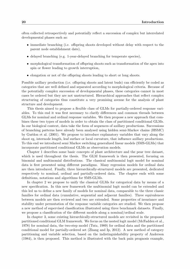
often collected retrospectively and potentially reflect a succession of complex but interrelateddevelopmental phases such as:
• immediate branching (i.e. offspring shoots developed without delay with respect to theparent node establishment date),
• delayed branching (e.g. 1-year-delayed branching for temperate species),
• morphological transformation of offspring shoots such as transformation of the apex intospin or flower leading to growth interruption,
• elongation or not of the offspring shoots leading to short or long shoots.
Possible axillary production (i.e. offspring shoots and latent buds) can efficiently be coded ascategories that are well defined and separated according to morphological criteria. Because ofthe potentially complex succession of developmental phases, these categories cannot in mostcases be ordered but they are not unstructured. Hierarchical approaches that reflect complexstructuring of categories thus constitute a very promising avenue for the analysis of plantstructure and development.
This thesis aimed to propose a flexible class of GLMs for partially-ordered response vari-ables. To this end it was first necessary to clarify differences and common threads betweenGLMs for nominal and ordinal response variables. We then propose a new approach that com-bines these two types of models in order to obtain the class of partitioned conditional GLMs.In our biological context, data take the form of sequences of axillary productions. Successionsof branching patterns have already been analysed using hidden semi-Markov chains (HSMC)by Guedon et al. (2001). We propose to introduce explanatory variables that vary along theshoot eg, internode length, leaf surface or local curvature, that influence axillary productions.To this end we introduced semi Markov switching generalized linear models (SMS-GLMs) thatincorporate partitioned conditional GLMs as observation models.
Chapter 1 describes some basic concepts of plant architecture and the pear tree dataset,which is used throughout the thesis. The GLM framework is then presented, focusing onbinomial and multinomial distributions. The classical multinomial logit model for nominaldata is first presented using different paradigms. Many regression models for ordinal dataare then introduced. Finally, three hierarchically-structured models are presented, dedicatedrespectively to nominal, ordinal and partially-ordered data. The chapter ends with somedefinitions, notations and algorithms for SMS-GLMs.
In chapter 2 we propose to unify the classical GLMs for categorical data by means of anew specification. In this new framework the multinomial logit model can be extended andthis led us to define a new family of models for nominal data, comparable to the three classicfamilies for ordinal data (cumulative, sequential and adjacent families). Three equivalencesbetween models are then reviewed and two are extended. Some properties of invariance andstability under permutation of the response variable categories are studied. We then proposea new method of supervised classification illustrated using three benchmark datasets. Finally,we propose a classification of the different models along a nominal/ordinal scale.
In chapter 3, some existing hierarchically-structured models are revisited in the proposedpartitioned conditional GLM framework. We focus on the nested logit model (McFadden et al.,1978) for nominal data, the two-step model (Tutz, 1989) for ordinal data and the partitionedconditional model for partially-ordered set (Zhang and Ip, 2012). A new method of categorypartitioning and variable selection, based on the indistinguishability property of Anderson(1984), is then proposed. This method is illustrated with the back pain prognosis example,
Introduction 21
previously analysed by Anderson (1984). Finally, our methodology for partially-ordered datais illustrated using a pear tree dataset.
Chapter 4 corresponds to the application of the statistical models investigated in thisthesis to plant architecture. The branching pattern of a shoot may be influenced by manyfactors that vary along the shoot eg, internode length, leaf surface or local curvature. Weintroduce a generalization of hidden semi-Markov chains for categorical response variablesthat incorporates explanatory variables which vary with the index parameter. Using thismodel, we demonstrate the influence of shoot growth pattern on its immediate branching.
Chapter 5 presents works in progress and perspectives. We first focus on the convergenceof Fisher’s scoring algorithm for some particular GLMs. A particular invariance propertypresented in chapter 2 is studied in depth. We then propose to represent the different GLMsfor categorical data using graph theory. Finally we propose an extension of the conditionallogit model (McFadden, 1973) which can be viewed as a family of qualitative choice models,whose implementation is not yet available.
Chapters 2, 3 and 4, corresponding to the original contribution of this thesis have beenwritten as pre-publications which has led to some redundancy between these chapters (mainlybetween chapters 2 and 3). All the statistical models developed in this thesis were implementedin C++ with a Python interface. They will be available soon as a Python module within theOpenAlea software platform: https://www.openalea.gforge.inria.fr

Chapter 1
State of the art
This chapter describes state of the art method for both plant architecture and statisticalmodelling. The biological context is presented, introducing some basic concepts of plantarchitecture. The pear tree dataset, which will illustrate almost all the models introduced inthis thesis, is described. The GLM framework for categorical response variable is then revisited,starting from GLM for univariate response with a focus on binary response variable, and is thengeneralizing to the multivariate case. The multinomial logit model is then presented as a GLMfor multivariate response and also as a qualitative choice model. The cumulative, sequentialand adjacent approaches for ordinal data are described, along with underlying motivationsand details on maximum likelihood estimation. The stereotype model is presented as anextension of the multinomial logit model for ordinal response variables. Finally, we presentthree regression models for hierarchically structured data. They share a partitioned conditionalstructure appropriate for different scales: nominal, ordinal and partially-ordered scales. Thischapter ends with some definitions, notations and algorithms about semi-Markov switchinggeneralized linear models (SMS-GLMs). These integrative models are used in chapter 4 toanalyse branching patterns and shoot growth, in apple and pear tree datasets.
Contents
1.1 Biological context . . . . . . . . . . . . . . . . . . . . . . . . . . . . . . . 24
1.2 Generalized Linear Models . . . . . . . . . . . . . . . . . . . . . . . . . . 27
1.2.1 Generalized linear models for univariate response variables . . . . . . . . 27
1.2.2 Generalized linear models for multivariate response variable . . . . . . . . 33
1.3 Logit model for nominal data . . . . . . . . . . . . . . . . . . . . . . . . 35
1.3.1 GLM for nominal response . . . . . . . . . . . . . . . . . . . . . . . . . . 36
1.3.2 Baseline-category logit model . . . . . . . . . . . . . . . . . . . . . . . . . 36
1.3.3 Qualitative choice model . . . . . . . . . . . . . . . . . . . . . . . . . . . . 36
1.4 Generalized linear models for ordinal data . . . . . . . . . . . . . . . . 39
1.4.1 Cumulative models . . . . . . . . . . . . . . . . . . . . . . . . . . . . . . . 39
1.4.2 Sequential models . . . . . . . . . . . . . . . . . . . . . . . . . . . . . . . 41
1.4.3 Adjacent models . . . . . . . . . . . . . . . . . . . . . . . . . . . . . . . . 42
1.4.4 Stereotype models . . . . . . . . . . . . . . . . . . . . . . . . . . . . . . . 44
1.5 Partitioned conditional generalized linear models . . . . . . . . . . . . 45
1.5.1 Nested logit model . . . . . . . . . . . . . . . . . . . . . . . . . . . . . . . 46
1.5.2 Two-step model . . . . . . . . . . . . . . . . . . . . . . . . . . . . . . . . 47
1.5.3 Partitioned conditional model for partially-ordered set . . . . . . . . . . . 49
1.6 Semi-Markov switching generalized linear models for categorical data 49
1.6.1 Hidden semi-Markov chains . . . . . . . . . . . . . . . . . . . . . . . . . . 50
1.6.2 Semi-Markov switching generalized linear models . . . . . . . . . . . . . . 53
24 1. State of the art
1.1 Biological context
This section is largely based on Godin and Caraglio (1998) andBarthelemy and Caraglio (2007).The notion of plant topological structure is based on the idea of decomposing a plant intoelementary constituents and describing their connections. To obtain natural decompositions,it is possible to take advantage of the fact that plants are modular organisms: plants can bedecomposed into sets of constituents of identical nature, such as internodes, axes, etc. Thetopological structure stemming from a modular decomposition consists of a description of theconnections between modules. The different modularities that can be observed in plants arethe outcome of the plant growth process.
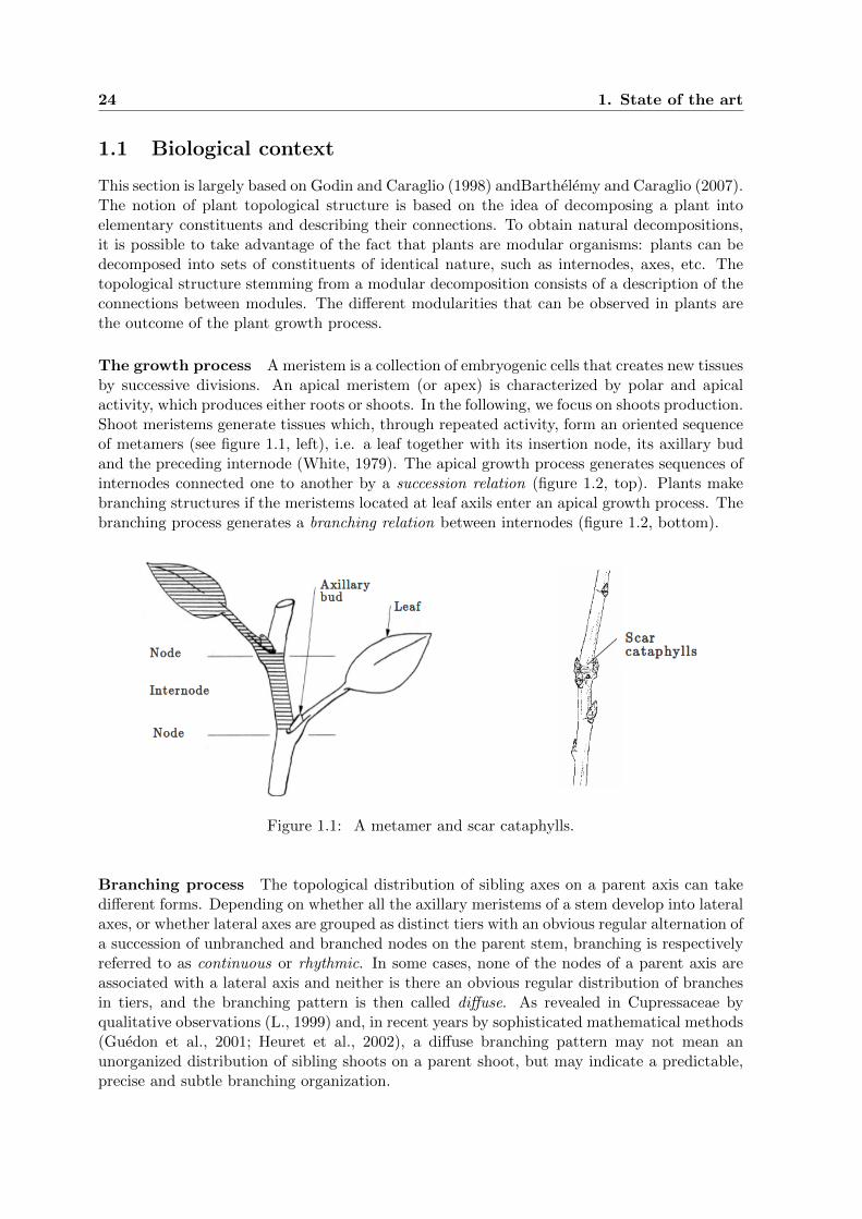
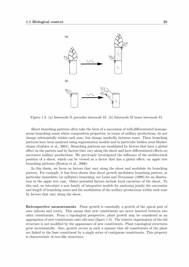
The growth process A meristem is a collection of embryogenic cells that creates new tissuesby successive divisions. An apical meristem (or apex) is characterized by polar and apicalactivity, which produces either roots or shoots. In the following, we focus on shoots production.Shoot meristems generate tissues which, through repeated activity, form an oriented sequenceof metamers (see figure 1.1, left), i.e. a leaf together with its insertion node, its axillary budand the preceding internode (White, 1979). The apical growth process generates sequences ofinternodes connected one to another by a succession relation (figure 1.2, top). Plants makebranching structures if the meristems located at leaf axils enter an apical growth process. Thebranching process generates a branching relation between internodes (figure 1.2, bottom).
Figure 1.1: A metamer and scar cataphylls.
Branching process The topological distribution of sibling axes on a parent axis can takedifferent forms. Depending on whether all the axillary meristems of a stem develop into lateralaxes, or whether lateral axes are grouped as distinct tiers with an obvious regular alternation ofa succession of unbranched and branched nodes on the parent stem, branching is respectivelyreferred to as continuous or rhythmic. In some cases, none of the nodes of a parent axis areassociated with a lateral axis and neither is there an obvious regular distribution of branchesin tiers, and the branching pattern is then called diffuse. As revealed in Cupressaceae byqualitative observations (L., 1999) and, in recent years by sophisticated mathematical methods(Guedon et al., 2001; Heuret et al., 2002), a diffuse branching pattern may not mean anunorganized distribution of sibling shoots on a parent shoot, but may indicate a predictable,precise and subtle branching organization.
1.1 Biological context 25
Figure 1.2: (a) Internode I1 precedes internode I2. (b) Internode I3 bears internode I4.
Shoot branching patterns often take the form of a succession of well-differentiated homoge-neous branching zones where composition properties, in terms of axillary productions, do notchange substantially within each zone, but change markedly between zones. These branchingpatterns have been analysed using segmentation models and in particular hidden semi-Markovchains (Guedon et al., 2001). Branching patterns are modulated by factors that have a globaleffect on the pattern and by factors that vary along the shoot and have differentiated effects onsuccessive axillary productions. We previously investigated the influence of the architecturalposition of a shoot, which can be viewed as a factor that has a global effect, on apple treebranching patterns (Renton et al., 2006).
In this thesis, we focus on factors that vary along the shoot and modulate its branchingpattern. For example, it has been shown that shoot growth modulates branching pattern, inparticular immediate (or sylleptic) branching; see Lauri and Terouanne (1998) for an illustra-tion in the apple tree case. Other potential factors include local curvature of the shoot. Tothis end, we introduce a new family of integrative models for analysing jointly the successionand length of branching zones and the modulation of the axillary productions within each zoneby factors that vary along the shoot.
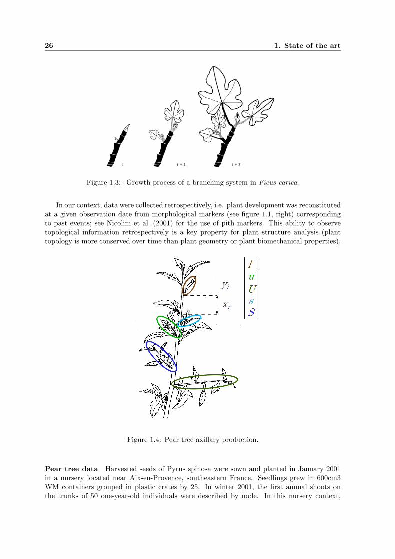
Retrospective measurements Plant growth is essentially a growth of the apical part ofaxes (shoots and roots). This means that new constituents are never inserted between twoolder constituents. From a topological perspective, plant growth may be considered as anaggregation of new constituents onto old ones (figure 1.3). The relative organization of the oldstructure is not modified by the appearance of new constituents. Plant topological structuresgrow incrementally. Also, growth occurs in such a manner that all constituents of the plantare linked to the base constituent by a single series of contiguous constituents. This propertyis characteristic of tree-like structures.
26 1. State of the art
Figure 1.3: Growth process of a branching system in Ficus carica.
In our context, data were collected retrospectively, i.e. plant development was reconstitutedat a given observation date from morphological markers (see figure 1.1, right) correspondingto past events; see Nicolini et al. (2001) for the use of pith markers. This ability to observetopological information retrospectively is a key property for plant structure analysis (planttopology is more conserved over time than plant geometry or plant biomechanical properties).
Figure 1.4: Pear tree axillary production.
Pear tree data Harvested seeds of Pyrus spinosa were sown and planted in January 2001in a nursery located near Aix-en-Provence, southeastern France. Seedlings grew in 600cm3WM containers grouped in plastic crates by 25. In winter 2001, the first annual shoots onthe trunks of 50 one-year-old individuals were described by node. In this nursery context,
1.2 Generalized Linear Models 27
individuals were able to grow twice a year, and the annual shoots were made up of one ortwo growth units (GU) - i.e. portion of the axis developed during an uninterrupted period ofgrowth - referred to as GU1 or GU2 in the following. Seven monocyclic annual shoots (GU1only) and 43 bicyclic annual shoots (GU1 and GU2) were observed.
The presence at each successive node of an immediate axillary shoot – i.e. developedwithout delay with respect to the parent node establishment date – was noted. Immediateshoots were classified in four categories according to length and transformation or not of theapex into spine (i.e. definite growth or not). The final dataset was thus made up of 50bivariate sequences of cumulative length 3285 combining a categorical variable Y (type ofaxillary production selected from among latent bud (l), unspiny short shoot (u), unspiny longshoot (U), spiny short shoot (s) and spiny long shoot (S)), with an interval-scaled variable X(internode length). Axillary production of the pear tree is shown in figure 1.4.
1.2 Generalized Linear Models
A categorical response variable needs to be considered as multivariate in the GLM framework.This section revisits the basis of GLMs for univariate and multivariate response using twoparametrizations of the exponential distribution family: the standard parametrization Nelderand Wedderburn (1972) and that described by Dobson (2002).
1.2.1 Generalized linear models for univariate response variables
The general parametrization of the linear predictor is first introduced in the context of thesimple linear model. This linear model is then generalized using the enlarged exponentialfamily of distributions and the link function is introduced. We chose to present the exponentialdistributions family with two parametrizations and give some hint concerning the link function.Fisher’s scoring algorithm is described and a property of canonical models reviewed. Finally,GLMs for binary and binomial response variable are detailed.
Let us consider the situation of regression analysis, with the univariate response variableY and the vector of Q explanatory variables X = (X1, . . . , XQ). We are interested in theconditional distribution of Y |X, observing values (yi, xi)i=1,...,n of the pair (Y,X). The vec-tor of explanatory variables may be deterministic (e.g. fixed by experimental conditions) orstochastic. All the response variables Yi are supposed to be conditionally independent of eachother, given Xi = xi. The dependence on xi is expressed through the linear predictor ηi.
The linear predictor When all the explanatory variables are quantitative (discrete orcontinuous) the linear predictor is
η = α+ xtδ,
where α ∈ R is the intercept and δ ∈ RQ is the vector of slopes.
When an explanatory variable is categorical, it has to be coded using dummy variables.A single categorical observed variable with M different possible categories is transformedinto an indicator vector x of dimension M − 1. This means that the mth component ofx = (x1, . . . , xM−1)t is defined by
xm =
1 if the category m is observed,0 else,
28 1. State of the art
and x is the null vector if category M is observed. The interaction between two explanatoryvariables xq and xh can be added using the product xqxh (Cartesian product if both arecategorical). The linear predictor η can be written as the scalar product of the design vectorzt = (1, xt) and the parameter vector βt = (α, δt)
η = ztβ,
where α ∈ R is the intercept and δ ∈ Rp is the vector of slopes.
Some equality constraints between the different slopes, called contrasts, can also be added.For example, considering the linear predictor η = α+ δ1x1 + δ2x2 with contrast δ1 = 3δ2, thereduced design vector z = (1, 3x1 +x2) can be used instead of the design vector zt = (1, x1, x2).A contrast can be interpreted as a transformation of explanatory variables. It should be notedthat in the case of Q explanatory variables, with all the categorical explanatory variables beingtransformed and possible interactions and contrasts being added, the dimension p of the vectorx is not necessarily equal to Q (in fact p ≥ Q).
Linear model For the classical linear model, the response variables Yi are normally dis-tributed given Xi = xi
Yi|Xi = xi ∼ N (µi, σ2),
where the mean parameter µi is a linear transformation of xi, through the design vector zi
µi = ztiβ,
where β ∈ R1+p and σ2 ∈ R+ are unknown parameters. Given a normal response variable Yand a vector of explanatory variable x, a linear model is fully specified by the design vector z.
The linear model assumes that the response distribution is continuous. Generalized linearmodels were introduced by Nelder and Wedderburn (1972) to relax this assumption and inparticular to take account of categorical and count response variables. In this framework, thedistribution of the response variable is assumed to belong to the exponential family, whichincludes the normal distribution.
1.2.1.1 Exponential family of distributions
The exponential family includes many well-known distributions such as the normal and gammadistributions for continuous variables, and the Poisson and binomial distributions for discretevariables. The density of a distribution, belonging to the exponential family, can be writtenin two different ways.
The first and most usual way (Nelder and Wedderburn, 1972) expresses the density functionf in terms of the natural parameter θ
f(y; θ) = exp
yθ − b(θ)
φω + c(y, φ)
, (1.1)
where
θ is the natural parameter,
b and c are specific functions corresponding to each distribution,
φ is the nuisance or dispersion parameter and ω is a known weight.
1.2 Generalized Linear Models 29
Property 1. Let Y be a random variable whose distribution belongs to the exponential family(1.1). The function b is assumed to be twice differentiable.
(i) E(Y) = b′(θ),
(ii) Cov(Y) =φ
ωb′′(θ).
For each distribution of the exponential family, θ is a particular reparametrization of itsmean µ. The second way (Dobson, 2002) expresses the density function f in terms of µ
f(y;µ) = exp a(y)θ(µ) + b(µ) + c(y) , (1.2)
where a, b, c and θ are known functions. If a is the identity function, the distribution is saidto be canonical, and θ(µ) is called the natural parameter. Three parts can be identified in thiswriting: the first depends on y and µ, the second on µ, and the third on y.
Property 2. Let Y be a random variable whose distribution belongs to the exponential family(1.2). The functions θ and b are assumed to be twice differentiable.
(i) E[a(Y)] = − b′(µ)
θ′(µ),
(ii) Cov[a(Y)] =θ′′(µ)b′(µ)− θ′(µ)b′′(µ)
[θ′(µ)]3.
Link function For a simple linear model the conditional expectation µ and the linear pre-dictor η = ztβ are directly related. For a generalized linear model, they have to be related bya particular function g, called the link function
g : M −→ R,µ 7−→ η,
because the space M is not necessarily R. In fact, the linear predictor η potentially liesbetween −∞ and +∞, while the mean parameter µ lies in a particular unidimensional spaceM depending on the response variable distribution. Thus the link function takes differentforms according to the constraints on spaceM. In the simple case of the normal distribution,there is no constraint on M (µ lies between −∞ and +∞) and therefore g is the identityfunction. For each distribution of the exponential family, the natural parameter θ can be seenas a particular function of µ; see parametrization (1.2). This function is called the canonicallink function. All GLMs defined with the canonical link are easy to estimate because thelikelihood is strictly concave (see next paragraph for details).
We have seen that the generalisation of the linear model, using the enlarged exponentialfamily of distributions, is used to define the link function. Finally, a GLM for univariateresponse variables is fully specified by
• the response variable distribution belonging to the exponential family,
• the design vector z,
• the link function g.
30 1. State of the art
Maximum likelihood estimation Parameter β is estimated by maximizing the log-likelihoodl. For the linear model, the equation ∂l/∂β = 0 has an analytic solution. For other GLMs,the equation ∂l/∂β = 0 is not linear with respect to β because of the link function. Thus,optimisation algorithms, such as the Newton-Raphson algorithm or Fisher’s scoring algorithm,are used to approximate β. Fisher’s scoring algorithm is given, at iteration m+ 1, by
β[m+1] = β[m] −
E
(∂2l
∂βt∂β
)β=β[m]
−1(∂l
∂β
)β=β[m]
.
For the sake of simplicity, the algorithm is detailed for only one observation (y, x) and thereforel = logP (Y = y|X = x;β). Using the chain rule, the score is given by
∂l
∂β=∂η
∂β
∂µ
∂η
∂θ
∂µ
∂l
∂θ.
Using Property 1 we obtain
∂l
∂β= z
(∂g
∂µ
)−1 1
V(Y |x)(y − µ),
and Fisher’s information matrix
Ey
(∂2l
∂βt∂β
)= −z
(∂g
∂µ
)−1 1
V(Y |x)
(∂g
∂µ
)−1
zt. (1.3)
It should be noted that the link function g must be invertible and inverse g−1 must be differ-entiable in order to obtain the score and Fisher’s information matrix. Moreover, g−1 must bestrictly monotone to easily interpret explanatory effect through estimated parameter β. Thelink function g :M→ R is thus generally assumed to be a diffeomorphism.
This algorithm ensures convergence towards the global maximum for any initial parameterβ[0], when the loglikelihood is strictly concave. For the canonical link function, the observedinformation matrix J (θ) = ∂2l/∂βt∂β and Fisher’s information matrix I(θ) = Ey[J (θ)] co-incide. Therefore, for the canonical link function, the observed information matrix J (θ) isnegative definite; see (1.3). Thus, the log-likelihood is strictly concave.
1.2.1.2 Bernoulli and binomial distributions
We focus here on GLMs for binary response variables.
Bernoulli distribution as a member of the exponential family Response variablesare measured on a binary scale and coded by 0 or 1. The axillary production of a plant, forinstance, may be qualified by the presence (y = 1) or absence (y = 0) of an axillary shoot.Success and failure are used as generic terms for the two categories. Let the binary randomvariable Y follow the Bernoulli distribution with parameter π ∈ [0, 1] with probability function
P (Y = y) = πy(1− π)1−y,
where y ∈ 0, 1. This is denoted by Y ∼ Ber(π). This probability function can be rewrittenas
P (Y = y) = exp
y log
(π
1− π
)+ log(1− π)
,
which is of the form (1.1) with b(θ) = log 1 + exp(θ) and of the form (1.2) with b(π) =log(1− π).
1.2 Generalized Linear Models 31
Binomial distribution as a member of the exponential family A binary variable isobserved repeatedly n times and focus is made on the number of successes, assuming indepen-dence between repetitions. For example, y is the number of axillary shoots along n successivenodes, and consequently, n−y is the number of latent buds. Let the discrete variable Y followthe binomial distribution with parameters n ∈ N∗ and π ∈ [0, 1] with probability function
P (Y = y) =
(n
y
)πy(1− π)n−y,
where y ∈ 0, . . . , n. This is denoted by Y ∼ B(n, π). This probability function can berewritten as
P (Y = y) = exp
y log
(π
1− π
)+ n log(1− π) + log
(n
y
),
which is of the form (1.1) with
θ = log
(π
1− π
),
ω = φ = 1,
b(θ) = n log 1 + exp(θ),
c(y, φ) = log
(n
y
),
and of the form (1.2) with
θ(π) = log
(π
1− π
),
a(y) = y,
b(π) = n log(1− π),
c(y) = log
(n
y
).
In the GLM framework, the mean is related to the linear predictor. For the binomialdistribution, even if the mean is nπ, the parameter of interest is just π. In fact, the parametern is involved in the function c of (1.1) and (1.2). However this function must be independentof the mean µ. The response variable has then to be slightly transformed. The binomialdistribution is expressed in terms of proportion y = y/n. The form of the distribution remainsthe same; only the support changes since for n trials y takes values in 0, . . . , n, whereas ytakes values in 0, 1/n, . . . , 1. The distribution of y is called scaled binomial distribution andis noted Y ∼ B(n, π)/n. The expectation of Y is now π. The scaled binomial distributionbelongs to the exponential family since for y ∈ 0, 1/n, . . . , 1 we have
P (Y = y) = exp
ny log
(π
1− π
)+ n log(1− π) + log
(n
ny
).
It should be noted that the number n = nx of observed data (y, x) changes according to thedifferent levels of explanatory variable x. Therefore the response variable y takes values indifferent sets 0, 1/nx, . . . , 1. Therefore, nx independent response variables with Bernoullidistributions Ber(π(x)) are more appropriate in the GLM framework than a single responsevariable with a scaled binomial distribution B(nx, π(x))/nx.
Link function for binary response For the Bernoulli distribution, π lies within the unitinterval [0, 1] and thus the identity link function is not suitable. The inverse of a cumulativedistribution function F is more appropriate. In fact, the link function g must be a diffeomorfismbetweenM and R. This holds for the Bernoulli case if the inverse link function g−1 is a strictlyincreasing and continuous cumulative distribution function F . Therefore M is the open unitinterval ]0, 1[.

32 1. State of the art
Canonical link function The canonical link is the logit function
g(π) = log
(π
1− π
)The inverse canonical link is the cumulative logistic distribution function
g−1(η) = F (η) =exp(η)
1 + exp(η)
Finally, the classical logit model has the following form
log
(π
1− π
)= ztβ,
or equivalently
π =exp(ztβ)
1 + exp(ztβ).
Alternative link functions Common choices of link function are presented here, alldefined by the inverse of classical cdfs. We consider models of the form
F−1(π) = ztβ,
or equivalently
π = F (ztβ).
A widely used model, particularly in econometrics, is the probit model based on the standardnormal distribution
φ(η) =1√2π
∫ η
−∞exp(−t2/2)dt.
In practice, the probit and logit models yield approximately the same results. Since φ is notanalytically defined, the logit model is often preferred, parameters having simple interpretationin terms of log-odds. Another conventional model is the complementary log-log model, definedwith the inverse cdf of the minimum extreme value distribution
F (η) = 1− exp − exp(η) ,
also referred to as the Gumbel min distribution. Unlike the logistic and normal distributions,the Gumbel min distribution is not symmetric. Another model can therefore be directlyobtained with the symmetric cdf F (η) = 1 − F (−η) corresponding to the maximum extremevalue distribution
F (η) = exp − exp(−η) ,
also referred to as the Gumbel max distribution. The corresponding model is called the log-logmodel. The Cauchy distribution characterized by its heavy tails can also be used
F (η) = tan−1(η)/π + 1/2,
where π ' 3.14159. Finally the exponential distribution can be used
F (η) = 1− exp(−η),
1.2 Generalized Linear Models 33
bearing in mind that the linear predictor η must be strictly positive in this case.
It should be noted for all these cdfs that if the location parameter u and the scale parameters are modified we have
Fu,s(η) = F
(η − us
)= F
(α− us
+ xtδ
s
),
and we obtain an equivalent model using the reparametrization α′ = (α− u)/s and δ′ = δ/s.
Finally, a GLM for a Bernoulli response variable is fully specified by:
• the design vector z,
• the cdf F .
Fisher’s scoring algorithm If f denotes the density function corresponding to cdf F , thescore is given by
∂l
∂β= f(η)
y − F (η)
F (η)[1− F (η)]z,
and Fisher’s information matrix is given by
E
[∂2l
∂βT∂β
]= − f2(η)
F (η)[1− F (η)]zzt.
The log-likelihood is strictly concave for the logit canonical link. This is not the case for otherlinks because the observed information matrix I(θ) depends on observation y. Wedderburn(1976) has shown that the log-likelihood for the normal and the Gumbel min distributions isstrictly concave. More generally, strict concavity of the log-likelihood holds if F and 1 − Fare strictly log-concave. It should be noted that concavity in β is equivalent to concavity in ηbecause
∂2l
∂βt∂β=∂2l
∂η2zzt.
Finally, distinguishing the two cases y = 1 and y = 0, the loglikelihood is either ln(F )or ln(1− F ). Using results from convex analysis, the strict log-concavity of F and 1− F canbe also shown for Gumbel max and Laplace distributions, but not for Student distributions(Bergstrom and Bagnoli, 2005).
1.2.2 Generalized linear models for multivariate response variable
The categorical distribution (with more than two categories), and the multinomial distributioncannot be written using the univariate exponential forms (1.1) and (1.2). The exponentialfamily has to be defined in the multivariate case. Let us consider a random vector Y ofRK whose distribution depends on a parameter θ ∈ RK . The distribution belongs to theexponential family if it can be written as (generalization of the form (1.1))
f(y; θ, φ) = exp
ytθ − b(θ)
φω + c(y, φ)
, (1.4)
where b, c are known functions, φ is the dispersion parameter, ω is a known weight and θ is thenatural parameter. It should be noted that the product between y and θ is a scalar product.

34 1. State of the art
Property 3. Let Y be a random vector whose distribution belongs to the exponential family(1.4). The function b is assumed to be twice differentiable with respect to θ.
(i) E(Y) = ∇b(θ),
(ii) Cov(Y) =φ
ωHb(θ).
where ∇b(θ) denotes the gradient and Hb(θ) the Hessian matrix of b with respect to θ.
As with Dobson, we propose to generalize the parametrization (1.2) for the multivariatecase
f(y; θ) = expa(y)tθ(µ) + b(µ) + c(y)
, (1.5)
where a, θ are known functions from RK to RK and b, c are known functions from RK to R.We also propose to generalize Property 2 in the multivariate case.
Property 4. Let Y be a random vector whose distribution belongs to the exponential family(1.5). The Jacobian matrix Jθ(µ) is assumed to be defined and invertible and the function bis assumed to be twice differentiable.
(i) E[a(Y)] = −J −1θ (µ)∇b(µ)
(ii) Cov[a(Y)] = J −1θ (µ)
( ∂2θ
∂µj∂µi
)tJ −1θ (µ)∇b(µ)
i,j
−Hb(µ)
J −tθ (µ)
See appendix A for the proof, which is a generalisation of Dobson’s proof (Dobson, 2002).
1.2.2.1 Multinomial distribution
Let J ≥ 2 denote the number of categories of the response variable and n ≥ 1 the number oftrials. Let π1, . . . , πJ denote the probabilities of each category, such that
∑Jj=1 πj = 1. The
discrete vector Y follows the multinomial distribution
Y ∼M(n, (π1, . . . , πJ)),
with∑J
j=1 yj = n. In the GLM framework, as only the probabilities πj are on interest, we focuson the case n = 1. Moreover, only J−1 probabilities πj are required to define the distribution(see chapter 2 for more details). Therefore, the truncated vector Y = (Y1, . . . , YJ−1)t and itsexpectation π = (π1, . . . , πJ−1)t are introduced. One observation y is an indicator vector ofthe observed category (the null vector corresponding to the last category). The distributionfunction is written in terms of y
f(y;π) =
J−1∏j=1
πyjj
1−J−1∑j=1
πj
1−∑J−1
j=1 yj
.
The natural parameter θ = (θ1, . . . , θJ−1)t is defined by
θ =
(log
(π1
1−∑J−1
j=1 πj
), . . . , log
(πJ−1
1−∑J−1
j=1 πj
))t,
and
b(θ) = log
1 +
J−1∑j=1
eθj
.
1.3 Logit model for nominal data 35
Thus, the density function is
f(y; θ) = expytθ − b(θ).
Using the weight ω = 1, the dispersion parameter φ = 1 and the null function c(y, λ) = 0,we see that this distribution function belongs to the exponential family of dimension K =dim(Y ) = dim(θ) = dim(π) = J − 1.
1.2.2.2 Canonical link function
The canonical link function for categorical GLMs is
g : M −→ RJ−1
π 7−→ η ,
such that
gj(π) = log
(πj
1−∑J−1
k=1 πk
),
for j = 1, . . . , J − 1, where M =π ∈]0, 1[J−1|
∑J−1j=1 πj < 1
. The linear predictor is now a
vector η = (η1, . . . , ηJ−1) and thus we must use a design matrix Z = Z(x) instead of a designvector z
η = Zβ.
Finally, a GLM for a categorical response variable is fully specified by
• the design matrix Z,
• the link function g = (g1, . . . , gJ−1).
1.2.2.3 Fisher’s scoring algorithm
For categorical GLMs, since the mean parameter π and the linear predictor are multivariate,the score is given by
∂l
∂β= Zt
∂π
∂ηCov(Y |x)−1 [y − π], (1.6)
where the Jacobian matrix ∂π/∂η depends on the link function. Therefore, in the following,we will simply detail the computation of this matrix for different link functions. It should benoted that the score, for the canonical link, is simplified as follows
∂l
∂β= Zt[y − π].
1.3 Logit model for nominal data
The multinomial logit model is the most commonly used regression model for nominal responsevariables. The probability of category j is given by
P (Y = j|x) =exp(αj + xtδj)∑Jk=1 exp(αk + xtδk)
,

36 1. State of the art
for j = 1, . . . , J . A reference category, for example the last one, must be arbitrarily chosen andcorresponding parameters αJ and δJ are assumed to be zero in order to avoid identifiabilityproblems. We thus obtain
P (Y = j|x) =exp(αj + xtδj)
1 +∑J−1
k=1 exp(αk + xtδk), (1.7)
for j = 1, . . . , J −1. This model has been introduced into biology, sociology and econometrics,with different definitions. It can be viewed as a GLM for multivariate responses, as J −1 logitmodels with the same reference category, or as a random utility model.
1.3.1 GLM for nominal response
We have seen that a GLM for categorical response variables is fully specified by the designmatrix Z and the link function g. The multinomial logit model is defined by the canonicallink function and the following design matrix
Z =
1 xt
. . .. . .
1 xt
,
with J − 1 rows and (J − 1)(1 + p) columns. See Fahrmeir and Tutz (2001) for more detailsabout this definition of the multinomial logit model.
1.3.2 Baseline-category logit model
In this framework, log odds for all(J2
)pairs of categories are described. Given a particular
subset of J − 1 log odds, the complementary subset is implicitly described. In fact, a base-line category must be chosen and the J − 1 other proportions πj are related to the baselineproportion. For example, using the last category J as baseline, we have
log
(πjπJ
)= αj + xtδj ,
for j = 1, . . . , J − 1. The effects change according to the response paired with the baseline.These J − 1 equations also determine parameters for logits with other pairs since
log
(πjπk
)= log
(πjπJ
)− log
(πkπJ
),
for j, k ∈ 1, . . . , J − 1. See Agresti (2002) for more details about this definition of themultinomial logit model.
1.3.3 Qualitative choice model
In qualitative choice models the statistical individual i is a consumer, the variable Y is thechoice of a consumer among J alternatives, and x is the vector of attributes. Two approacheslead to the multinomial logit model: Luce’s choice axiom and the principle of random utilitymaximisation.
1.3 Logit model for nominal data 37
Luce’s choice axiom
Luce (1959) defined an axiom for qualitative choice models. This axiom is based on twofundamental properties: choice is probabilistic and the probability of choosing an alternativefrom one set is related to the probability of choosing the same alternative from a different set.Let C denote a finite set of alternatives and PB(j) the conditional probability of choosing thealternative j given the subset of alternatives B ⊂ C. Luce’s choice axiom is defined by thetwo following partsPart 1: if Pj,k ∈]0, 1[ for all j, k ∈ C with j 6= k, then for A ⊂ B ⊂ C
PC(A) = PB(A)PC(B),
Part 2: if Pj,k = 0 for some j, k ∈ C with j 6= k, then for B ⊂ C
PC(B) = PC\j(B \ j).
The second part, which is useful when some alternatives are never chosen in pairwise choices,is often ignored. It should be noted that the first part is not formally a conditional probabilitybecause this axiom does not assume that C is a universal set. Using Luce’s choice axiom(part 1) for a subset of two alternatives A = j, k, we obtain the independence of irrelevantalternative (IIA) property
Pj,k(j)
Pj,k(k)=PB(j)
PB(k),
for all subsets B such that j, k ⊂ B.
Luce (1959) showed that his axiom implies the existence of strictly positive values vj foreach alternative j ∈ C such that for all B ⊂ C and all j ∈ B we have
PB(j) =vj∑k∈B vk
.
As the quantities vj are strictly positive, there exists real values ηj such that
PB(j) =exp(ηj)∑k∈B exp(ηk)
,
for all B ⊂ C and all j ∈ B.
Principle of random utility maximisation
In probabilistic choice theory, it is often assumed that for each consumer i, an unobservedutility Ui,j is associated with the jth alternative. In this framework, a rational consumer i willchoose the alternative j that provides the highest utility Ui,j
Yi = j ⇔ Ui,j = max1≤k≤J
Ui,k.
Although it is assumed that choices are made rationally, not every characteristic of the in-dividual or choice situation that affects choice behaviour can be measured. Therefore, therandom utility Ui,j has the following form
Ui,j = ηi,j + εi,j ,
38 1. State of the art
where ηi,j is the structural part and εi,j is the random part. The residuals εi,j are independentlyidentically distributed random variables with cdf H and density function h. If this choicebehaviour situation holds, Y is determined by the principle of random utility maximisationand we obtain a random utility model (RUM).
Marschak (1960) and McFadden (1973) showed that the multinomial logit model is a RUM.In fact, the probability of alternative j for one consumer is
P (Y = j) = P
⋂k 6=jUj ≥ Uk
= P
⋂k 6=jεk ≤ ηj − ηk + εj
P (Y = j) =
∫ +∞
−∞
∏k 6=j
H (ηj − ηk + e)
h(e)de.
The last equality holds because the residuals εj are independently and identically distributed.Finally, if we make the assumption of a Gumbel max distribution for residuals εj , we obtain
P (Y = j) =exp(ηj)∑Jk=1 exp(ηk)
,
for j = 1, . . . , J .
Different parametrizations of logit models
Depending on the form of the linear predictors ηj , we obtain different logit models:
• Multinomial logit model: ηj = αj + xtδj . Here the attributes are the same for allalternatives and the parameters depend on each alternative.
• Conditional logit model: ηj = α + xtjδ. Here the attributes are dependent on eachalternative and the parameters are the same for all alternatives.
• Universal logit model: ηj = αj + xtjδj . Here the attributes and the parameters aredependent on each alternative.
These three types of logit models respect the principle of random utility maximisation. Theyalso satisfy Luce’s choice axiom and consequently share the IIA property. The ratio of proba-bilities for alternatives j and k
P (Y = j)
P (Y = k)= exp(ηj − ηk)
does not depend on other alternatives. This property is sometimes too restrictive to modelindividual choice behaviour, as explained by Debreu (1960) with the well known example ofblue and red buses.
1.4 Generalized linear models for ordinal data 39
1.4 Generalized linear models for ordinal data
As noted by Agresti (2010), the results obtained with the multinomial logit model are invari-ant under permutations of the response variable categories. Therefore, the multinomial logitmodel does not utilize all information because the ordering of categories is ignored. Moreoveroften more parameters than are really needed are involved in the model. Models devoted toordinal data are expected to be more parsimonious and have simpler interpretations than themultinomial logit model.
This section describes the cumulative, sequential and adjacent approaches for ordinal data.For each approach we present the model in its original logit form and in general form. Wedescribe the latent regression model and give detail on the maximum likelihood estimation inthe general case (except for the adjacent approach). The stereotype logit model (Anderson,1984) is presented as an extension of the multinomial logit model which requires ordinalconstraints on parameters. The indistinguishability procedure introduced by Anderson (1984)for an ordinal response variable is also described.
1.4.1 Cumulative models
1.4.1.1 Cumulative logits
For J categories with associated probabilities π1, . . . , πJ , the cumulative logits are defined by
logit P (Y ≤ j) = log
P (Y ≤ j)P (Y > j)
= log
π1 + . . .+ πjπj+1 + . . .+ πJ
,
for j = 1, . . . , J − 1. The cumulative proportional logit model is then defined by relatingcumulative logits to proportional linear predictors
logit P (Y ≤ j|x) = αj + xtδ,
for j = 1, . . . , J − 1. It should be noted that the logit difference has the simple form
logit P (Y ≤ j|x1) − logit P (Y ≤ j|x2) = log
P (Y ≤ j|x1)/P (Y > j|x1)
P (Y ≤ j|x2)/P (Y > j|x2)
= δt(x1 − x2).
We can see that the log odds ratio does not depend on category j and is proportional to thedistance between x1 and x2. Because of this proportional odds property, the cumulative logitmodel is also called the proportional odds logit model (McCullagh, 1980).
1.4.1.2 Latent variable motivation
The proportional odds model can be defined using a latent variable to simplify its interpretation(McCullagh, 1980). Let Y be a latent continuous variable and a1, . . . , aJ−1 be strictly-orderedcut points. The response events can also be expressed in terms of the latent variable Y
Y = j ⇔ aj−1 < Y ≤ aj ,
for j = 1, . . . , J with a0 = −∞ and aJ = +∞ by convention. The order is more easily inter-pretable using the latent continuous variable, where the ordered categories are now considered
40 1. State of the art
as successive intervals ]aj−1, aj ]. A linear regression model can then be defined, considering Yas the response variable
Yi = a+ xtib+ εi, (1.8)
where the residuals εii=1,...,n are independent and identically distributed random variableswith cdf F . Finally, the cumulative probabilities for one individual are
P (Y ≤ j|x) = P (Y ≤ aj)= P
(ε ≤ aj − a− xtb
)P (Y ≤ j|x) = F (αj + xtδ) (1.9)
with αj = aj − a, and δ = −b. This latent variable motivation leads naturally to theparametrization ηj = αj − xtδ (used for example in the polr package in R). Using the lo-gistic cdf as residual distribution, we obtain the odds proportional logit model.
Grouped Cox model. Using the Gumbel min distribution for the residual εi of latentmodel (1.8), we obtain the grouped Cox model. In this case (1.9) becomes
P (Y ≤ j|x) = 1− exp− exp(αj + xtδ), (1.10)
for j = 1, . . . , J − 1. This is equivalent to
log [− logP (Y > j|x)] = αj + xtδ,
for j = 1, . . . , J − 1, with the complementary log-log link.
Cumulative models can also be defined without the proportionality assumption. We canuse any design matrix Z such that the corresponding linear predictors ηj(x) are strictly orderedfor any observed values x. Finally, a cumulative model is fully specified by
• the design matrix Z,
• the cdf F .
1.4.1.3 Fisher’s scoring algorithm
Only the Jacobian matrix ∂π/∂η depends on the link function in the score equation of multi-nomial GLM (1.6). For cumulative models (1.9), we have πj = F (ηj)− F (ηj−1), and thus thegeneral term of the Jacobian matrix is
∂πj∂ηi
=
f(ηj) if i = j,−f(ηj−1) if i = j − 1,0 otherwise,
for row i and column j, where f denotes the density function f = F ′.
It has been shown that concavity of the log-likelihood holds for cumulative proportionalmodels if F , 1−F and f are log-concave (Pratt, 1981; Burridge, 1981). Using results of convexanalysis, the strict log-concavity of F , 1−F and f can be shown for logistic, normal, Gumbelmin, Gumbel max and Laplace distributions, but not for Student distributions (Bergstromand Bagnoli, 2005).
1.4 Generalized linear models for ordinal data 41
1.4.2 Sequential models
1.4.2.1 Sequential logits
For J categories with associated probabilities π1, . . . , πJ , the sequential logits are defined by
logit P (Y = j|Y ≥ j) = log
P (Y = j)
P (Y > j)
= log
πj
πj+1 + . . .+ πJ
,
for j = 1, . . . , J − 1. The sequential proportional logit model is then defined by relatingsequential logits to proportional linear predictors
logit P (Y = j|Y ≥ j;x) = αj + xtδ,
for j = 1, . . . , J − 1.
1.4.2.2 Latent variables motivation
The sequential proportional model can also be motivated by latent random variables (Tutz,1991). Let (Yi,j)j=1,...,J−1 be a random sequential continuous process for each individual i suchthat for j = 1, . . . , J − 1
Yi,j = a+ xtib+ εi,j , (1.11)
where the residuals εi,jj=1,...,J−1i=1,...,n are independent and identically distributed random vari-
ables with cdf F and corresponding density function f . For one individual, (Yj)j=1,...,J−1 isa sequential binary mechanism. At each step j, if the continuous variable Yj exceeds cutpoint aj , then the process continues, otherwise the process is stopped. The event Y = joccurs if the latent process have been stopped at step j. Therefore, the event Y = j can bedecomposed into j latent events
Y = j ⇔j−1⋂t=1
Yt > at⋂Yj ≤ aj.
The conditional event Y = j|Y ≥ j may also be expressed as
Y = j|Y ≥ j ⇔ Yj ≤ aj,
leading to model
P (Y = j|Y ≥ j;x) = F (αj + xtδ), (1.12)
with αj = aj − a, and δ = −b. Using the logistic cdf as residual distribution, we obtain theodds proportional logit model.
Proportional hazard model. Using the Gumbel min distribution for the residual εi oflatent model (1.11), we obtain the proportional hazard model. In this case (1.12) becomes
P (Y = j|Y ≥ j;x) = 1− exp− exp(αj + xtδ), (1.13)
for j = 1, . . . , J − 1. This is equivalent to
log [− logP (Y > j|Y ≥ j;x)] = αj + xtδ,
for j = 1, . . . , J−1, with the complementary log-log link. This model is the categorical versionof the continuous hazard model (Cox, 1972). It is also called the grouped Cox model.
42 1. State of the art
Equivalence between sequential and cumulative models. Equivalence between thesequential form (1.13) and the cumulative form (1.10) of the grouped Cox model has beenshown by Laara and Matthews (1985), using the following parametrization α′j = log
j∑
k=1
exp(αj)
for j = 1, . . . , J − 1,
δ′ = δ.
Equivalence between the sequential and cumulative non-proportional models, with the ex-ponential cdf F (η) = 1 − exp(−η), has been shown by Tutz (1991), using the followingparametrization
α′1 = α1,δ′1 = δ1,
and
α′j = αj − αj−1,
δ′j = δj − δj−1,for j = 2, . . . , J − 1.
Caution should be exercised for this last model because it is defined only for positive valuesof the linear predictors ηj .
Sequential models can also be defined without the proportionality assumption. Any designmatrix Z may be used and there are no constraints on corresponding linear predictors. Finally,a sequential model is fully specified by:
• the design matrix Z,
• the cdf F .
1.4.2.3 Fisher’s scoring algorithm
Using the score equation of multinomial GLM (1.6), we see that only the Jacobian matrix∂π/∂η must be computed. For sequential models (1.12), we have πj = F (ηj)
∏j−1k=11−F (ηk),
and thus the general term of the Jacobian matrix is
∂πj∂ηi
=
f(ηj)
j−1∏k=1
1− F (ηk) if i = j,
−f(ηi)F (ηj)
j−1∏k=1,k 6=i
1− F (ηk) if i < j,
0 otherwise,
for row i and column j.
1.4.3 Adjacent models
1.4.3.1 Adjacent logits
For J categories with associated probabilities π1, . . . , πJ , the adjacent logits are defined by
logit P (Y = j|Y ∈ j, j + 1) = log
P (Y = j)
P (Y = j + 1)
= log
πjπj+1
,
1.4 Generalized linear models for ordinal data 43
for j = 1, . . . , J−1. The adjacent proportional logit model is then defined by relating adjacentlogits to proportional linear predictors
logit P (Y = j|Y ∈ j, j + 1;x) = αj + xtδ,
for j = 1, . . . , J − 1. The adjacent logit model is defined by relating adjacent logits to non-proportional linear predictors
logit P (Y = j|Y ∈ j, j + 1;x) = αj + xtδj ,
for j = 1, . . . , J − 1. Even if there is no latent variable motivation, it is possible to define anadjacent model for any cdf F
P (Y = j|Y ∈ j, j + 1;x) = F (ηj),
with different possible parametrization of ηj . The Newton-Raphson algorithm is detailed forthe adjacent logit models by Agresti (2010). In the same manner as for sequential models, theconditional form of adjacent models implies independence between all linear predictors ηj . Noconstraints are required on η to obtain non-negative probabilities. Finally, an adjacent modelis fully specified by
• the design matrix Z,
• the cdf F .
1.4.3.2 Equivalence with baseline-category logit model
The connection between the adjacent logit model and the baseline-category logit model wasdescribed by Agresti (2010). If we assume that the distribution of Y |X = x is defined by anadjacent logit model, then we have
log
(πjπJ
)= log
(πjπj+1
× . . .× πJ−1
πJ
)=
J−1∑k=j
ηk
=
J−1∑k=j
αk + xt
J−1∑k=j
δk
= α′j + xtδ′j ,
for j = 1, . . . , J − 1. Agresti (2010) noted also that if the adjacent logit has a proportionalform, then we obtain a baseline-category logit model with the parametrization
δ′j =
J−1∑k=j
δk =
J−1∑k=j
δ = (J − j)δ,
for j = 1, . . . , J − 1 .
44 1. State of the art
1.4.4 Stereotype models
Instead of defining new logit ratios of probabilities, Anderson (1984) conserved the baseline-category logit structure but proposed a new predictor parametrization. Thus he used themodel
log
(πjπJ
)= αj + xtδj , (1.14)
with additional constraints on δj , for j = 1, . . . , J − 1. Using different parametrizations ofpredictors ηj , Anderson proposed a flexible logistic regression model useful for d-dimensionalor ordered regression relationships. He defined a procedure to test the distinguishability ofsuccessive categories with respect to explanatory variables x.
1.4.4.1 Dimensional regression relation
The multinomial logit model is defined only with the complete parametrization ηj = αj +xtδj .For a given explanatory vector x of dimension p in the most general form, this is the maximalpossible parametrization with (J − 1)(1 + p) parameters. We could define the multinomiallogit model with the proportional parametrization ηj = αj + xtδ. Taking into account x,this is the minimal possible parametrization, with J − 1 + p parameters. With this in mind,Anderson proposed a large set of parametrizations to cover the range between minimal andmaximal parametrizations. Thus he used model (1.14) with a particular parametrization forthe J − 1 slopes δj . First, Anderson proposed to relax slightly the proportional assumption(δ1 = . . . = δJ−1 = δ) using the parametrization
δj = φjδ, (1.15)
for j = 1, . . . , J − 1, where φj are scalars. To avoid identifiability problems, the number ofparameters must be less than the number of parameters of the maximal model
(J − 1)2 + p ≤ (J − 1)(1 + p).
This is the case for J > 2 and p > 1. Otherwise, if J = 2 or p = 1, one scalar must be fixed(φ1 = 1 such as in Anderson (1984)). He referred to model (1.14) with parametrization (1.15)as the one-dimensional stereotype model. He then proposed the two-dimensional stereotypemodel using parametrization
δj = φjδ + ψjγ,
for j = 1, . . . , J−1. Finally, he defined the d-dimensional stereotype model using parametriza-tion
δj =d∑
k=1
φk,jγk,
for j = 1, . . . , J − 1, where φk,j ∈ R and γk ∈ Rp. The number of different slopes γk issuch that d ≤ J − 1 for identifiability issues. Therefore, the maximal number of identifiablescale parameters φk,j is J − 1 − d. Anderson proposed the maximal dimension d = min(J −1, p). Finally, using the flexibility of slope parametrization in two ways (scale parameters φk,jand slope parameters γk), Anderson proposed a multinomial logit model with any numberof parameters between the minimal and the maximal number of parameters (i.e. between(J − 1 + p) and (J − 1)(1 + p)).
1.5 Partitioned conditional generalized linear models 45
1.4.4.2 Ordered regression relation
Anderson proposed to order the parameters (φj)j=1,...,J of the one-dimensional stereotypemodel to obtain an ordered regression relation
1 = φ1 > φ2 > . . . > φJ = 0.
It should be noted that Anderson did not use this ordering as an a priori constraint. If theestimated parameters φj are ordered, then the order is considered as a consequence of theestimation. As noticed by Tutz (2012), the stereotype model cannot be considered to be anordinal model, even though it is used for ordinal response variables in applications.
1.4.4.3 Indistinguishability procedure
Anderson (1984) proposed a testing procedure - useful for ordinal data - to identify successivecategories that can be clearly distinguished by the explanatory variables x. These categoriesare said to be indistinguishable with respect to x when the explanatory variables x do not havesignificantly different effects on them. He proposed to aggregate the corresponding successiveslope parameters δj and use a deviance test. More precisely, he proposed an iterative proce-dure to find the best splitting point among categories 1, . . . , J with respect to x. The minimalnumber of splitting point is zero, corresponding to the simple model without explanatory vari-ables (null hypothesis H0), and the maximal number of splitting points is J−1, correspondingto the classical multinomial logit model with J − 1 different slopes.
The first step is to find the best split into two groups of categories. The hypothesis H(2;r)
is then introducedH(2;r) : δ1 = . . . = δr; δr+1 = . . . = δJ = 0,
for r = 1, . . . , J − 1. Comparing the corresponding log-likelihood values l(2;r) yields the bestsplitting point r∗ such that l2 = l(2;r∗) = maxr l(2;r). The hypothesis H(2;r∗) is then testedagainst H0, using the deviance statistic 2(l2 − l0) which follows a χ2
p distribution under H0.Finally, if the splitting point r∗ is accepted, the procedure must be restarted in parallel forthe two groups 1, . . . , r∗ and r∗ + 1, . . . , J in order to obtain the best partition into threegroups.
This is a dichotomous partitioning procedure with at most J(J−1)/2 different parametriza-tions to test. It should be noted that this procedure is simplified for the one-dimensionalstereotype model since the equality between slopes δ1 = . . . = δr becomes equality betweenscalar parameters φ1 = . . . = φr. In practice, only this particular case of the procedure isused.
1.5 Partitioned conditional generalized linear models
The main idea is to recursively partition the J categories then specify a conditional GLMat each step. This is why this type of models is called partitioned conditional GLMs. Suchmodels have already been proposed, e.g. the nested logit model (McFadden et al., 1978), thetwo-step model (Tutz, 1989) and the partitioned conditional model for partially-ordered sets(POS-PCM) (Zhang and Ip, 2012). In a first level, the entire set of categories is partitionedinto L groups (or “nests”) as follows
1, . . . , J =
L⋃l=1
Nl,
46 1. State of the art
and in a second level, the groups are partitioned into categories. Thus, a basic event isdecomposed as follows
Y = j ⇔ Y ∈ Nl ∩ Y = j|Y ∈ Nl.
Partitioning step The groups Nl are considered as categories and a categorical regressionmodel is used to describe the probabilities P (Y ∈ Nl|x) for l = 1, . . . , L.
Conditioning step For each group Nl, the response variable Y is conditioned on Nl and aGLM is used to describe the conditional probabilities P (Y = j|Y ∈ Nl;x) for j ∈ Nl.
More generally, this partitioning/conditioning process may be reiterated for Nl. However,these models have been formally defined and used with only two or three levels. The first aimof these models is to aggregate the categories that are influenced by the same explanatoryvariable.This is very similar to the principle of distinguishability defined by Anderson. Thenested logit model were introduced in this way. The categories are aggregated according tothe explanatory variable. On the other hand, the two-step model takes account of the orderassumption among the categories, aggregating only successive categories. A more recent aimwas to use the partial ordering among the categories to define an adapted partitioned condi-tional model. For any partially-ordered structure, Zhang and Ip (2012) proposed a particularrecursive partition which “conserves” the order relation.
1.5.1 Nested logit model
The most well known partitioned conditional model for nominal data is the nested logit modeldefined by McFadden et al. (1978) in the framework of individual choice behaviour. This modelwas introduced to avoid the inconsistency of the independence of irrelevant alternatives (IIA)property in some situations. Let us illustrate this inconsistency with the classical example ofblue and red buses (Debreu, 1960). Assume we are interested in urban travel demand, withthe simple situation of two alternatives: A = blue bus, car. Suppose that the consumer hasno preference between the two alternatives; this means that PA(blue bus) = PA(car) = 1/2.Suppose now that the travel company adds some red buses and the consumer again has nopreference between blue and red buses; this means that PB(blue bus) = PB(red bus) whereB = blue bus, red bus, car. Using the IIA property we obtain
1 =PA(blue bus)
PA(car)=PB(blue bus)
PB(car).
Finally, we obtain PB(blue bus) = PB(red bus) = PB(car) = 1/3, whereas we expected theprobabilities PB(blue bus) = PB(red bus) = 1/4 and PB(car) = 1/2.
In this example the IIA property is not appropriate because two alternatives are verysimilar and also share many characteristics. The nested logit model captures the similaritiesbetween close alternatives by partitioning the choice set into “nests” (groups). Thus, theconsumer chooses first between bus and car according to price, travel time, . . . and secondlybetween the two buses according to preferred color. More generally, suppose that alternativescan be aggregated according to their similarities; this means that all alternatives of the samenest Nl share attributes xl, whereas other alternatives do not. In the following, the nested logitmodel is presented with only two levels. Let L be the number of nests obtained by partitioning
1.5 Partitioned conditional generalized linear models 47
the set of J alternatives.
1, . . . , J =L⋃l=1
Nl.
If j denotes an alternative belonging to the nest Nl, then the probability of alternative j isdecomposed as follows
P (Y = j|x) = P (Y = j|Y ∈ Nl;xl)P (Y ∈ Nl|x0, IV ), (1.16)
where IV = (IV1, . . . , IVL) denotes the vector of inclusive values described thereafter, x0 arethe attributes which influence only the first choice level between nests and x = (x0, x1, . . . , xL).Each probability of the product (3.3) is determined by a multinomial logit model as follows
P (Y = j|Y ∈ Nl;xl) =
exp(ηlj)∑k∈Nl
exp(ηlk),
and
P (Y ∈ Nl|x0, IV ) =exp(η0
l + λlIVl)L∑k=1
exp(η0k + λkIVk)
,
where
IVl = ln
∑k∈Nl
exp(ηlk)
.
The deterministic utilities (predictors) ηlj are function of attributes xl and η0l are function of
attributes x0. In practice they are linear with respect to x. In some situations the attributevalues depend on the alternative. For example, the travel price xj depends on the J alternativesbus, car, metro, etc. In this case, the conditional logit model was introduced by McFadden(1974), using the linear predictors ηj = αj + xtjδ for j = 1, . . . , J .
Because of the inclusive values, the nested logit model must be estimated in two steps.In the first step, the L models of the second level can be estimated separately because theparameters βl are different in each nest. The inclusive values IVl of each nest can then becomputed and used, in a second step, to estimate the first level model.
1.5.2 Two-step model
The two-step model, or compound model, was defined by Tutz (1989) to decompose the la-tent mechanism of an ordinal response into two levels. Ordinal-scale response variables arecommonly used in medicine and psychology for instance to assess a patient’s condition. Thisordinal scale is often built from a coarse and a fine scales. For the back pain prognosis datasetdescribed by Doran and Newell (1975), the response variable y is the assessment of back painafter three weeks of treatment using the six ordered categories: worse (1), same (2), slightimprovement (3), moderate improvement (4), marked improvement (5), complete relief (6).Categories 3, 4 and 5 can be aggregated into a general category improvement. Thus, the coarsescale corresponds to the categories: worse, same, improvement, complete relief, and the finescale corresponds to the categories: slight improvement, moderate improvement and markedimprovement (see figure 3.4).

48 1. State of the art
Figure 1.5: Two-scale back pain assessment.
Then, the model must be decomposed into two levels, corresponding to the coarse scaleand the fine scale. More generally, let N1, . . . , NL be a partition of the J categories, whichconserves the order relationship. The sets also have the form Nl = ml−1 + 1, . . . ,ml with0 = m0 < m1 < . . . < mL = J . The probability of each category j ∈ Nl is decomposed asfollows
P (Y = j) = P (Y ∈ Nl)P (y = j|Y ∈ Nl).
An advantage of the model is that different parameters are involved in different steps:
P (Y = j|x, β) = P (Y ∈ Nl|x, β1)P (y = j|Y ∈ Nl;x, β2).
The ordinal scale of the response variable is used and must be assumed. Therefore, Tutz (1989)defined the cumulative compound model and the sequential compound model, appropriate forordinal response variable.
1.5.2.1 Cumulative compound model
Here, we have two cumulative latent mechanisms for the two levels
coarse scale: P (Y ∈l⋃
k=1
Nk|x) = F (αl + xtδ) for l = 1, . . . , L
fine scale: P (Y ≤ j|Y ∈ Nl;x) = F (αlj + xtδl) for j ∈ Nl and l = 1, . . . , L
1.5.2.2 Sequential compound model
Here, we have two sequential latent mechanisms for the two levels
coarse scale: P (Y ∈ Nl|Y ∈L⋃k=l
Nk;x) = F (αl + xtδ) for l = 1, . . . , L
fine scale: P (Y = j|Y ≥ j;Y ∈ Nl;x) = F (αlj + xtδl) for j ∈ Nl and l = 1, . . . , L
An advantage of the two-step model is its simple structure. After rearranging the data, theparameters of each step may be estimated in parallel using classic algorithm for generalizedlinear models. Thus, no two-step estimation procedure is necessary unlike, for example, forthe nested logit model.
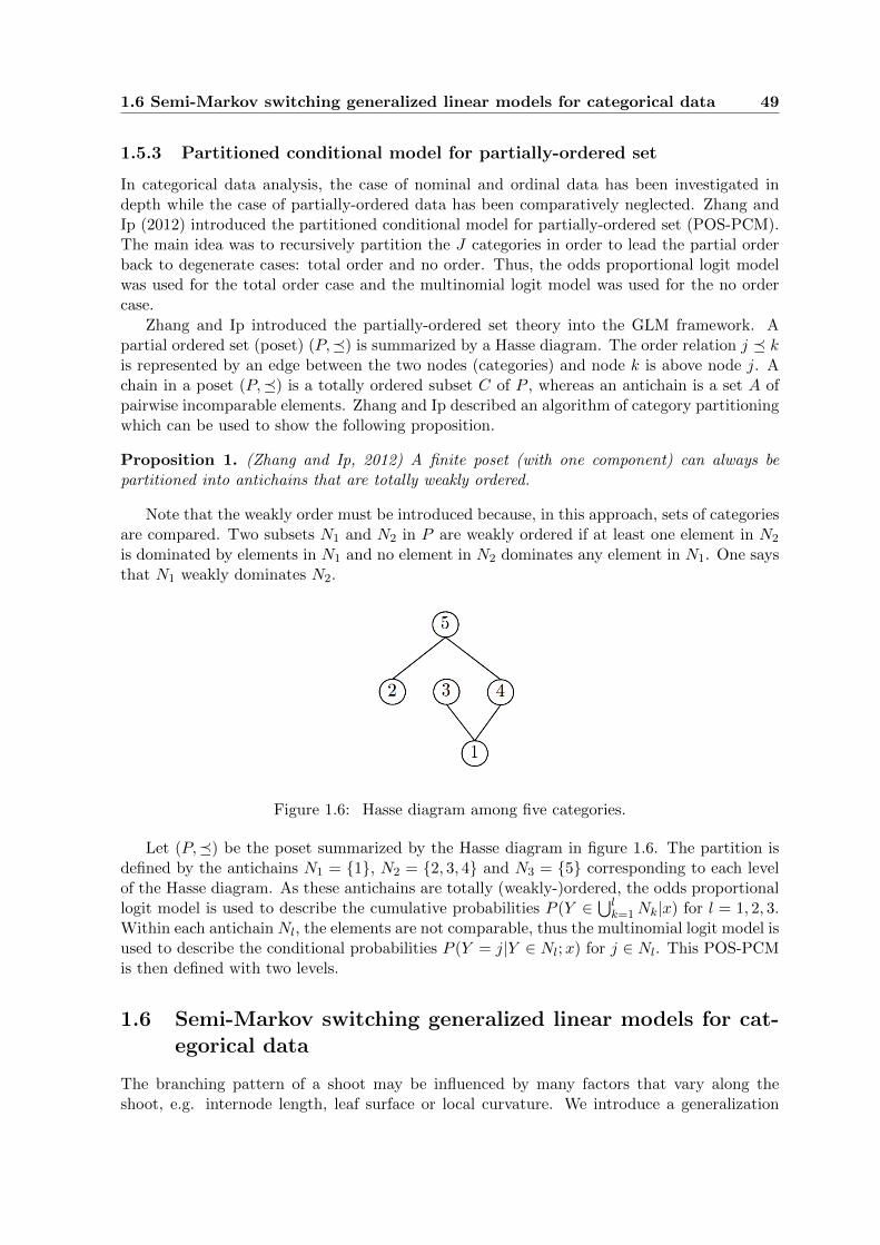
1.6 Semi-Markov switching generalized linear models for categorical data 49
1.5.3 Partitioned conditional model for partially-ordered set
In categorical data analysis, the case of nominal and ordinal data has been investigated indepth while the case of partially-ordered data has been comparatively neglected. Zhang andIp (2012) introduced the partitioned conditional model for partially-ordered set (POS-PCM).The main idea was to recursively partition the J categories in order to lead the partial orderback to degenerate cases: total order and no order. Thus, the odds proportional logit modelwas used for the total order case and the multinomial logit model was used for the no ordercase.
Zhang and Ip introduced the partially-ordered set theory into the GLM framework. Apartial ordered set (poset) (P,) is summarized by a Hasse diagram. The order relation j kis represented by an edge between the two nodes (categories) and node k is above node j. Achain in a poset (P,) is a totally ordered subset C of P , whereas an antichain is a set A ofpairwise incomparable elements. Zhang and Ip described an algorithm of category partitioningwhich can be used to show the following proposition.
Proposition 1. (Zhang and Ip, 2012) A finite poset (with one component) can always bepartitioned into antichains that are totally weakly ordered.
Note that the weakly order must be introduced because, in this approach, sets of categoriesare compared. Two subsets N1 and N2 in P are weakly ordered if at least one element in N2
is dominated by elements in N1 and no element in N2 dominates any element in N1. One saysthat N1 weakly dominates N2.
Figure 1.6: Hasse diagram among five categories.
Let (P,) be the poset summarized by the Hasse diagram in figure 1.6. The partition isdefined by the antichains N1 = 1, N2 = 2, 3, 4 and N3 = 5 corresponding to each levelof the Hasse diagram. As these antichains are totally (weakly-)ordered, the odds proportionallogit model is used to describe the cumulative probabilities P (Y ∈
⋃lk=1Nk|x) for l = 1, 2, 3.
Within each antichain Nl, the elements are not comparable, thus the multinomial logit model isused to describe the conditional probabilities P (Y = j|Y ∈ Nl;x) for j ∈ Nl. This POS-PCMis then defined with two levels.
1.6 Semi-Markov switching generalized linear models for cat-egorical data
The branching pattern of a shoot may be influenced by many factors that vary along theshoot, e.g. internode length, leaf surface or local curvature. We introduce a generalization
50 1. State of the art
of hidden semi-Markov chains for categorical response variables that incorporates explanatoryvariables that vary with the index parameter. Using this model, we demonstrate in chapter 4the influence of shoot growth pattern on its immediate branching.
We consider here a semi-Markov switching generalized linear model (SMS-GLM), which isa two-scale segmentation model. In this framework, the succession and length of branchingzones (coarse scale) are represented by a non-observable semi-Markov chain while the axillaryproductions within a branching zone, modulated by factors that vary along the shoot (finescale), are represented by generalized linear models attached to each state of the semi-Markovchain. A SMS-GLM combines three categories of variables: (i) “state” variable representingthe non-directly observable branching zones, (ii) plant response categorical variable (typesof axillary production), (iii) explanatory variables that vary with node rank (e.g., internodelength). In this section, we first review the hidden semi-Markov chains definition and esti-mation for the general case of any observation process. The estimation procedure is thendescribed in the case of a GLM as observation model.
1.6.1 Hidden semi-Markov chains
Let us first introduce semi-Markov chains by starting with simple Markov chains. The sequenceof state variables S0 = s0, . . . , St = st is denoted by St−1
0 = st−10 and the entire sequence
S0 = s0, . . . , ST−1 = sT−1 by S = s. A first-order Markov chain is a discrete-time discrete-state-space stochastic process characterized by the dependency relation
P (St = st|St−11 = st−1
1 ) = P (St = st|St−1 = st−1).
Definition 1. Let St be a first-order time-homogeneous Markov chain with finite statespace 0, . . . , A − 1 (simply referred to as Markov chain in the following). A Markov chainis defined by the following parameters:
• initial probabilities ϕa = P (S0 = a) with∑
a ϕa = 1,
• transition probabilities pa,b = P (St = b|St−1 = a) with∑
b pa,b = 1.
A major drawback of the Markov chain is the inflexibility in describing the time spentin given state, which is geometrically distributed. The implicit occupancy (or sojourn time)distribution of a nonabsorbing state j is the 1-shifted geometric distribution with parameter1− pa,a
da(u) = (1− pa,a)pu−1a,a (1.17)
This is the unique discrete memoryless distribution. A useful generalization of Markov chainslies in the class of semi-Markov chains in which the process moves out of a given state accordingto an embedded Markov chain with self-transition probability in non-absorbing states pa,a = 0and where the time spent in a given non-absorbing state is modelled by an explicit occupancydistribution. The possible parametric state occupancy distributions are binomial, negativebinomial and Poisson distributions with an additional shift parameter d ≥ 1 which defines theminimum sojourn time in a given state.
Definition 2. (Guedon, 2003) A semi-Markov chain is constructed from an embeddedfirst-order Markov chain. This A-state first-order Markov chain is defined by the followingparameters:
• initial probabilities ϕa = P (S0 = a) with∑
a ϕa = 1.
1.6 Semi-Markov switching generalized linear models for categorical data 51
• transition probabilities
– non absorbing state a: ∀b 6= a, pa,b = P (St = b|St 6= a, St−1 = a) with∑
b 6=a pa,b = 1and pa,a = 0,
– absorbing state a: pa,a = P (St = a|St−1 = a) = 1 and ∀b 6= a, pa,b = 0.
This embedded first-order Markov chain represents transitions between distinct states except inthe absorbing state case. An occupancy (or sojourn time) distribution is attached to each nonabsorbing state a of the embedded first-order Markov chain
da(u) = P (St+u+1 6= a, St+u−v = a, v = 0, . . . , u− 2|St+1 = a, St 6= a)
for u = 1, . . . , Ua, where Ua denotes the upper bound to the time spent in state a. Hence, weassume that the state occupancy distributions are concentrated on finite sets of time points.For the particular case of the last visited state, we need to introduce the survivor function ofthe sojourn time in state a, Da(u) =
∑v≥u da(u). The whole (first-order Markov chain +
state occupancy distributions) constitutes a semi-Markov chain.
Hidden Markov chains emerged in the 1970s in engineering and have since become a majortool for both pattern recognition applications, e.g. speech or handwriting recognition (see(Rabiner, 1989) for tutorial introductions), and biological sequence analysis (Churchill, 1989).
Hidden semi-Markov chains with non parametric state occupancy distributions were firstproposed in the field of speech recognition by Ferguson (1980). After this pioneering work, thestatistical inference problem related to hidden semi-Markov chains was further investigated bydifferent authors (Russell and Moore, 1985; Levinson, 1986; Guedon, 1992) and different para-metric hypotheses were put forward for the state occupancy distributions (Poisson, “discrete”gamma).
Definition 3. A hidden (semi-)Markov chain can be viewed as a pair of stochastic pro-cesses St, Yt where the output process Yt is related to the state process St, which is a(semi-)Markov chain, by a probabilistic function or mapping denoted by f (hence Yt = f(St)).Since the mapping f is such that a given output may be observed in different states, the stateprocess St is not observable directly but only indirectly through the output process Yt. Thisoutput process Yt is related to the (semi-)Markov chain St by the observation (or emis-sion) probabilities. The definition of observation probabilities expresses the assumption thatthe output process at time t depends only on the underlying Markov chain at time t. For eachstate a the observation distribution is denoted by ba
ba(y) = P (Yt = y|St = a) with∑y
ba(y) = 1.
It should be noted that an HMC can be interpreted as a finite mixture model with Marko-vian dependency. In the same way, an HSMC can be interpreted as a finite mixture modelwith semi-Markovian dependency.
Conditional independence and likelihood of HSMC
For an HMC, both relations of conditional independence hold
• St is independent of S0, Y0, . . . , St−2, Yt−2, Yt−1 given St−1, for all t > 0.
• Yt is independent of S0, Y0, . . . , St−1, Yt−1 given St, for all t ≥ 0.
52 1. State of the art
Thus, for an HMC, the likelihood of the joint process S,Y is
P (Y = y,S = s; θ) = P (Y = y|S = s)P (S = s)
= ϕs0
T−1∏t=1
pst−1,st
T−1∏t=0
bst(yt)
, (1.18)
where θ denotes the set of all HMC parameters (i.e. initial probabilities ϕa, transition proba-bilities pa,b and observed distributions ba for all a ∈ 0, . . . , A− 1).
By replacing a first-order Markov chain by a semi-Markov chain, the Markovian propertyis transferred to the level of the embedded first-order Markov chain. In the semi-Markov chaincase, the conditional independence between the past and the future is ensured only when theprocess moves from one state to another distinct state. This property holds at each time stepin the case of a Markov chain. For an HSMC, the likelihood of the joint process S,Y is
ϕs0ds0(u0)
R−1∏r=1
psr−1,srdsr(ur)
psR−1,sRDsR(uR)I
(R∑r=0
ur = T
)T−1∏t=0
bst(yt)
, (1.19)
where sr is the (r + 1)th visited state, ur is the time spent in state ur and I() denotes theindicator function; see for instance Russell and Moore (1985); Rabiner (1989).
Maximum likelihood estimation
In the following, the algorithm computation is described for only one observed sequence y.For an HMC, since the state sequence s is not observable, the likelihood is given by
L(y; θ) =∑s
P (Y = y,S = s; θ),
where∑
s means the sum on every possible state sequence of lenth T . This sum has exactly AT
elements and can be written as a matrices product (Altman, 2007). Therefore the likelihoodof an HMC can be directly maximized (Collings and Ryden, 1998; Turner, 2008).
The direct maximisation of the likelihood is more complex for an HSMC. In fact thelikelihood cannot be written as a matrix product
L(y; θ) =∑s
∑u
P (Y = y, ST−1+u0 = sT−1+u
0 ; θ),
where∑
u means the sum on every supplementary duration from time T spent in the stateoccupied at time T − 1. Since the state sequence s is not observable, a standard solution formaximum likelihood estimation is the EM algorithm.
EM algorithm for HSMC The EM algorithm was introduced by Dempster et al. (1977)to find maximum likelihood estimates of parameters when the model depends on unobservedlatent variables. Each iteration of the EM algorithm decomposes into two steps: the E step(Expectation) and the M step (Maximisation). In the following we describe these two steps atthe iteration k + 1 for an HSMC.
1.6 Semi-Markov switching generalized linear models for categorical data 53
E step The focus here is on the conditional expectation of the completed data log-likelihood given the observed data. Using equality (1.19), the conditional expectation can bewritten as a sum of four terms that depend on initial probabilities, transition probabilities,sojourn time distributions and observed distributions
Q(θ|θ[k]) = E
logP (yT1 , sT1 ; θ)Y = y; θ[k]
= Qϕ(ϕaA−1
a=0 |θ[k]) +
A−1∑a=0
Qp(pA−1a=0 |θ
[k])
+A−1∑a=0
Qd(da(u)|θ[k])I(pa,a = 0) +A−1∑a=0
Qb(ba(y)Y−1y=0 |θ
[k]) (1.20)
Guedon (2003) introduced a “forward-backward” algorithm for the E step, based on the fol-lowing decomposition
L1a(t) = P (St+1 6= a, St = a|Y = y)
=P (Y T
t+1 = yTt+1|St+1 6= a, St = a)
P (Y Tt+1 = yTt+1|Y t
1 = yt1)P (St+1 6= a, St = a|Y t
1 = yt1)
L1a(t) = Ba(t)Fa(t)
which expresses the conditional independence between the past and the future of the processat state change times (1.19). Guedon and Cocozza-Thivent (1990) showed that the quantitiesFa(t)
[k+1] (respectively L1a(t)[k+1]) can be computed by a forward (respectively backward)
pass through observed sequence y, using the previous values of parameters θ[k].
M step The reestimation formulas for the parameters of a HSMC are obtained by maxi-mizing the different terms of Q(θ|θ[k]) (see the decomposition (1.20)), each term depending ona given subset of θ. For each parameter subset, the reestimation formula is given in Guedon(2003). This formula is directly deduced from the maximization of the first three terms of(1.20). Therefore we obtain the next parameter values ϕ[k+1] and P [k+1] using the quanti-ties previously computed Fa(t)
[k+1] and L1a(t)[k+1]. The computation of quantities d[a+1],
corresponding to the sojourn time distribution in each state, is described by Guedon (2003).The update of observation model parameters (corresponding to quantities b[k+1] in the case ofsimple distribution) is detailed in the next subsection in the case of GLM for categorical data.
1.6.2 Semi-Markov switching generalized linear models
Here, the observation conditional Yt|Xt = xt is defined by several GLMs for categoricalresponse variables. In fact, one GLM is associated with each state a ∈ 0, . . . , A − 1 of theHSMC, corresponding to the observed distribution ba. These A distributions are characterizedby the parameters βa of the corresponding GLM. As we have seen previously, the estimationof these parameters is not related to the semi-Markov parameters estimation and thereforeonly the M step differs.
In the M step, the term of Q(θ|θ[k]) corresponding to an observation GLM is maximisedusing Fisher’s scoring algorithm. Therefore there are two levels of iterations: Fisher’s scoringiteration m being nested in EM iteration k. For the M step, we must maximise the conditionalexpectation Qb(ba(y)Y−1
y=0 |θ[k]) with respect to βa for each state a ∈ 0, . . . , A − 1. On the
54 1. State of the art
iteration m+ 1 we obtain for state a
β[m+1]a = β[m]
a −
E∂2Q(b| θ[k])
∂βa∂βta
βa=β
[m]a
−1∂Q(b|θ[k])
∂βa
βa=β
[m]a
For the EM algorithm, the conditional expectation Qb(ba(y)Y−1y=0 |θ[k]) has the following form
Qb(ba(y)Y−1y=0 |θ
[k]) =T−1∑t=0
L1[k]a (t) ba(yt|xt),
and thus we obtain∂Q(b|θ[k])
∂βa
βa=β
[m]a
=
T−1∑t=0
L1[k]a (t)
∂l(yt, xt)
∂βa
βa=β
[m]a
,
where Fisher’s score is computed as detailed by (1.6).
Chapter 2
A new specification of generalizedlinear models for categorical data
Abstract
Many regression models for categorical data have been introduced in a variety of applied fields,motivated by different paradigms but their specification are not homogeneous. Therefore, thesemodels are difficult to compare and their appropriateness with respect to category orderingassumptions is questionable. The first contribution of this chapter is to unify the classicalregression models for categorical response variables, whether nominal or ordinal. This uni-fication is based mainly on a decomposition of the link function into two parts: an inversecontinuous cdf and a ratio of probabilities. This allows us to define a new family of modelsfor nominal data, comparable to the cumulative, sequential and adjacent families of modelsused for ordinal data. We finally propose a classification of GLMs for categorical data alonga nominal/ordinal scale.
Keywords: link function, nominal variable, ordinal variable, model reparametrization, in-variance under permutation, stability under permutation.
Contents
2.1 Introduction . . . . . . . . . . . . . . . . . . . . . . . . . . . . . . . . . . 56
2.2 Exponential form of the categorical distribution . . . . . . . . . . . . . 57
2.3 Specification of generalized linear models for categorical data . . . . 58
2.3.1 Decomposition of the link function . . . . . . . . . . . . . . . . . . . . . . 58
2.3.2 (r,F,Z) specification of GLMs for categorical data . . . . . . . . . . . . . 59
2.3.3 Compatibility of the three components r, F and Z . . . . . . . . . . . . . 63
2.3.4 Fisher’s scoring algorithm . . . . . . . . . . . . . . . . . . . . . . . . . . . 64
2.4 Properties of GLMs for categorical data . . . . . . . . . . . . . . . . . 65
2.4.1 Equivalence between GLMs for categorical data . . . . . . . . . . . . . . . 65
2.4.2 Permutation invariance and stability . . . . . . . . . . . . . . . . . . . . . 69
2.5 Investigation of invariance properties using benchmark datasets . . 73
2.6 Applications . . . . . . . . . . . . . . . . . . . . . . . . . . . . . . . . . . 75
2.6.1 Supervised classification . . . . . . . . . . . . . . . . . . . . . . . . . . . . 75
2.6.2 Partially-known total ordering . . . . . . . . . . . . . . . . . . . . . . . . 78
2.7 Discussion . . . . . . . . . . . . . . . . . . . . . . . . . . . . . . . . . . . . 79

56 2. A new specification of generalized linear models for categorical data
2.1 Introduction
Since GLMs were first introduced by Nelder and Wedderburn (1972), many regression modelsfor categorical data have been developed and introduced into a variety of applied fields such asmedicine, econometrics and psychology. They have been motivated by different paradigms andtheir specifications are not homogeneous. Most have been defined for ordinal data (Agresti,2010), whereas only one has been defined for nominal data: the multinomial logit modelintroduced by Luce (1959) (also referred to as the baseline-category logit model (Agresti,2002)). The three classical models for ordinal data are the odds proportional logit model(McCullagh, 1980), the sequential logit model (Tutz, 1990) (also referred to as the continuationratio logit model (Dobson, 2002)), and the adjacent logit model (Masters, 1982; Agresti, 2010).They have been extended by either replacing the logistic cumulative distribution function (cdf)by other cdfs F (e.g. normal or Gumbel cdfs; see the grouped Cox model for instance, alsoreferred to as the proportional hazard model), or introducing different parametrizations ofthe linear predictor (i.e. changing the design matrix Z). No such developments have beenundertaken for the multinomial logit case, and one of our goals is to fill this gap.
It should be noted that the three previously mentioned models for ordinal data, and themultinomial logit model, all rely on the logistic cdf. The difference between them stems fromanother element in the link function. In fact, the four corresponding link functions can bedecomposed into the logistic cdf and a ratio of probabilities r. For the odds proportional logitmodel, the ratio corresponds to the cumulative probabilities P (Y ≤ j). Here, we proposeto decompose the link function of any GLM for categorical data into a cdf F and a ratio r.Using this decomposition it can be shown that all the models for ordinal data were definedby fixing the ratio r and changing the cdf F and the design matrix Z. For example, allthe cumulative models were obtained by fixing the cumulative probabilities P (Y ≤ j) as thecommon structure. In the same way, the two families of sequential and adjacent models weredefined with probability ratios P (Y = j|Y ≥ j) and P (Y = j|j ≤ Y ≤ j + 1). Now, we canextend the multinomial logit model by fixing only its ratio r and leaving F and Z unrestricted.
Our first contribution in this chapter (section 2.3) is to unify all these models by introducingthe new (r, F, Z)-triplet specification. Differences and commonalities between models are thushighlighted, making them easily comparable. In this framework, the multinomial logit modelis extended, replacing the logistic cdf by other cdfs. We thus obtain a new family of modelsfor nominal data, comparable to the three classical families of models used for ordinal data.We can now compare all the models according to the three components: ratio r for structure,cdf F for fit, and design matrix Z for parametrization.
Sections 2.4 & 2.5 investigate this comparison in depth by studying the equivalences be-tween models. We first revisit three equivalences between models with different ratios, shownby Laara and Matthews (1985), Tutz (1991) and Agresti (2010) then generalize two of them toobtain equalities between families of models. Some properties of invariance and stability un-der permutation of the response categories are then presented. “Models for nominal categoriesshould be invariant under arbitrary permutations [. . . ]. On the other hand, models for ordinaldata should be invariant only under the special reverse permutation” (McCullagh, 1978).
In section 2.6, using the extended family of models for nominal data, and their invarianceproperty, we introduce a family of supervised classifiers. In final section 2.7 we discuss the ap-propriateness of certain models with respect to category ordering assumptions. A classificationof the different models along a nominal/ordinal scale according to their invariance propertiesis then proposed. By also considering difficulties of interpretability and inference, we providesome advice concerning the practical choice of a model structure.
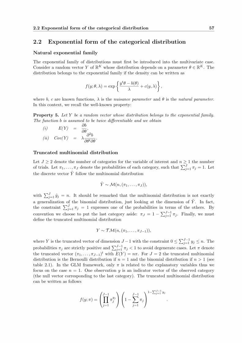
2.2 Exponential form of the categorical distribution 57
2.2 Exponential form of the categorical distribution
Natural exponential family
The exponential family of distributions must first be introduced into the multivariate case.Consider a random vector Y of RK whose distribution depends on a parameter θ ∈ RK . Thedistribution belongs to the exponential family if the density can be written as
f(y; θ, λ) = exp
ytθ − b(θ)
λ+ c(y, λ)
,
where b, c are known functions, λ is the nuisance parameter and θ is the natural parameter.In this context, we recall the well-known property:
Property 5. Let Y be a random vector whose distribution belongs to the exponential family.The function b is assumed to be twice differentiable and we obtain
(i) E(Y) =∂b
∂θ,
(ii) Cov(Y) = λ∂2b
∂θt∂θ.
Truncated multinomial distribution
Let J ≥ 2 denote the number of categories for the variable of interest and n ≥ 1 the numberof trials. Let π1, . . . , πJ denote the probabilities of each category, such that
∑Jj=1 πj = 1. Let
the discrete vector Y follow the multinomial distribution
Y ∼M(n, (π1, . . . , πJ)),
with∑J
j=1 yj = n. It should be remarked that the multinomial distribution is not exactly
a generalization of the binomial distribution, just looking at the dimension of Y . In fact,the constraint
∑Jj=1 πj = 1 expresses one of the probabilities in terms of the others. By
convention we choose to put the last category aside: πJ = 1 −∑J−1
j=1 πj . Finally, we mustdefine the truncated multinomial distribution
Y ∼ TM(n, (π1, . . . , πJ−1)),
where Y is the truncated vector of dimension J −1 with the constraint 0 ≤∑J−1
j=1 yj ≤ n. The
probabilities πj are strictly positive and∑J−1
j=1 πj < 1 to avoid degenerate cases. Let π denote
the truncated vector (π1, . . . , πJ−1)t with E(Y ) = nπ. For J = 2 the truncated multinomialdistribution is the Bernoulli distribution if n = 1 and the binomial distribution if n > 1 (seetable 2.1). In the GLM framework, only π is related to the explanatory variables thus wefocus on the case n = 1. One observation y is an indicator vector of the observed category(the null vector corresponding to the last category). The truncated multinomial distributioncan be written as follows
f(y;π) =
J−1∏j=1
πyjj
1−J−1∑j=1
πj
1−∑J−1
j=1 yj
.
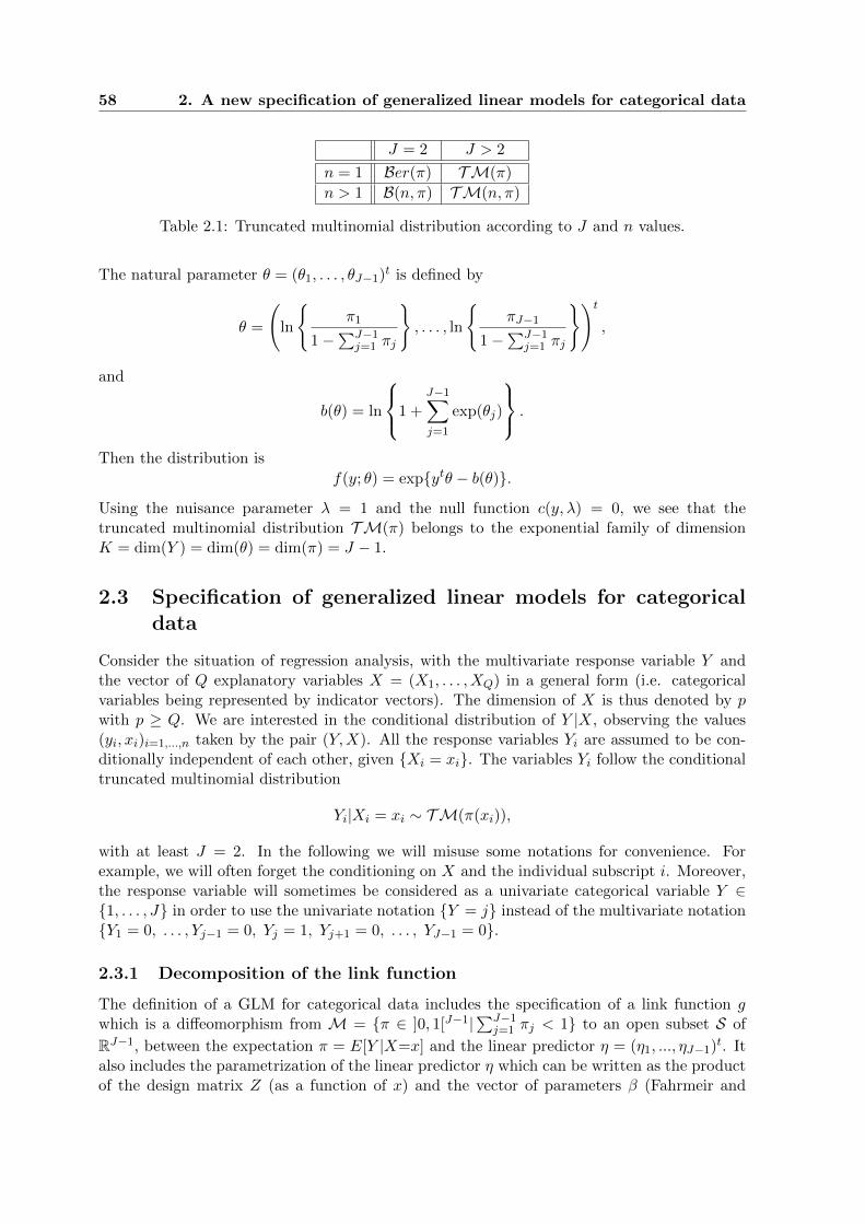
58 2. A new specification of generalized linear models for categorical data
J = 2 J > 2
n = 1 Ber(π) TM(π)
n > 1 B(n, π) TM(n, π)
Table 2.1: Truncated multinomial distribution according to J and n values.
The natural parameter θ = (θ1, . . . , θJ−1)t is defined by
θ =
(ln
π1
1−∑J−1
j=1 πj
, . . . , ln
πJ−1
1−∑J−1
j=1 πj
)t,
and
b(θ) = ln
1 +J−1∑j=1
exp(θj)
.
Then the distribution is
f(y; θ) = expytθ − b(θ).
Using the nuisance parameter λ = 1 and the null function c(y, λ) = 0, we see that thetruncated multinomial distribution TM(π) belongs to the exponential family of dimensionK = dim(Y ) = dim(θ) = dim(π) = J − 1.
2.3 Specification of generalized linear models for categoricaldata
Consider the situation of regression analysis, with the multivariate response variable Y andthe vector of Q explanatory variables X = (X1, . . . , XQ) in a general form (i.e. categoricalvariables being represented by indicator vectors). The dimension of X is thus denoted by pwith p ≥ Q. We are interested in the conditional distribution of Y |X, observing the values(yi, xi)i=1,...,n taken by the pair (Y,X). All the response variables Yi are assumed to be con-ditionally independent of each other, given Xi = xi. The variables Yi follow the conditionaltruncated multinomial distribution
Yi|Xi = xi ∼ TM(π(xi)),
with at least J = 2. In the following we will misuse some notations for convenience. Forexample, we will often forget the conditioning on X and the individual subscript i. Moreover,the response variable will sometimes be considered as a univariate categorical variable Y ∈1, . . . , J in order to use the univariate notation Y = j instead of the multivariate notationY1 = 0, . . . , Yj−1 = 0, Yj = 1, Yj+1 = 0, . . . , YJ−1 = 0.
2.3.1 Decomposition of the link function
The definition of a GLM for categorical data includes the specification of a link function gwhich is a diffeomorphism from M = π ∈ ]0, 1[J−1|
∑J−1j=1 πj < 1 to an open subset S of
RJ−1, between the expectation π = E[Y |X=x] and the linear predictor η = (η1, ..., ηJ−1)t. Italso includes the parametrization of the linear predictor η which can be written as the productof the design matrix Z (as a function of x) and the vector of parameters β (Fahrmeir and
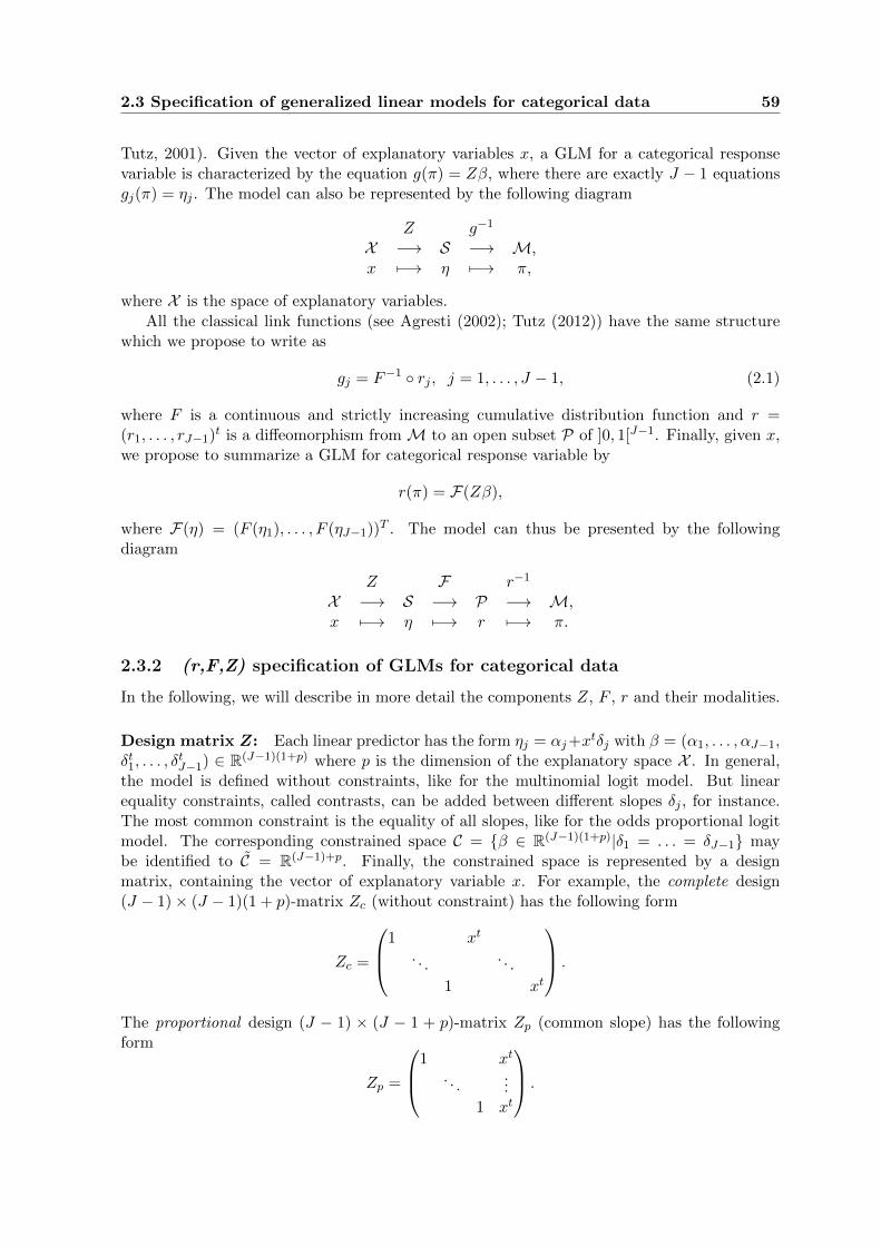
2.3 Specification of generalized linear models for categorical data 59
Tutz, 2001). Given the vector of explanatory variables x, a GLM for a categorical responsevariable is characterized by the equation g(π) = Zβ, where there are exactly J − 1 equationsgj(π) = ηj . The model can also be represented by the following diagram
Z g−1
X −→ S −→ M,x 7−→ η 7−→ π,
where X is the space of explanatory variables.
All the classical link functions (see Agresti (2002); Tutz (2012)) have the same structurewhich we propose to write as
gj = F−1 rj , j = 1, . . . , J − 1, (2.1)
where F is a continuous and strictly increasing cumulative distribution function and r =(r1, . . . , rJ−1)t is a diffeomorphism from M to an open subset P of ]0, 1[J−1. Finally, given x,we propose to summarize a GLM for categorical response variable by
r(π) = F(Zβ),
where F(η) = (F (η1), . . . , F (ηJ−1))T . The model can thus be presented by the followingdiagram
Z F r−1
X −→ S −→ P −→ M,x 7−→ η 7−→ r 7−→ π.
2.3.2 (r,F,Z) specification of GLMs for categorical data
In the following, we will describe in more detail the components Z, F , r and their modalities.
Design matrix Z: Each linear predictor has the form ηj = αj+xtδj with β = (α1, . . . , αJ−1,
δt1, . . . , δtJ−1) ∈ R(J−1)(1+p) where p is the dimension of the explanatory space X . In general,
the model is defined without constraints, like for the multinomial logit model. But linearequality constraints, called contrasts, can be added between different slopes δj , for instance.The most common constraint is the equality of all slopes, like for the odds proportional logitmodel. The corresponding constrained space C = β ∈ R(J−1)(1+p)|δ1 = . . . = δJ−1 maybe identified to C = R(J−1)+p. Finally, the constrained space is represented by a designmatrix, containing the vector of explanatory variable x. For example, the complete design(J − 1)× (J − 1)(1 + p)-matrix Zc (without constraint) has the following form
Zc =
1 xt
. . .. . .
1 xt
.
The proportional design (J − 1) × (J − 1 + p)-matrix Zp (common slope) has the followingform
Zp =
1 xt
. . ....
1 xt
.

60 2. A new specification of generalized linear models for categorical data
The model without slopes (δ1 = . . . = δJ−1 = 0), considered as the minimal response model,is defined with different intercepts αj (the design matrix is the identity matrix of dimensionJ − 1). In most cases, the design matrix contains the identity matrix as minimal block, suchas Zc and Zp. These two matrices are sufficient to define all the classical models. It shouldbe noted that for a given constrained space C, there are an infinity of corresponding designmatrices which will be considered as equivalent. For example
Z ′p =
1 −xt...
. . ....
1 . . . 1 −xt
is equivalent to Zp. In the following, the design matrices Zp and Zc are considered as therepresentative element of their equivalence class and the set of all possible design matrices Z,for a given vector of explanatory variables x, will be denoted by Z. This set Z contains alldesign matrices between Zp and Zc, with number of columns between J−1+p and (J−1)(1+p).
Cumulative distribution function F : The most commonly used symmetric distributionsare the logistic and normal distributions, but Laplace and Student distributions may also beuseful. The most commonly used asymmetric distribution is the Gumbel min distribution
F (η) = 1− exp − exp(η) .
Let F denote the symmetric of F (i.e. F (η) = 1−F (−η)). The symmetric of the Gumbel mindistribution is the Gumbel max distribution
F (η) = exp − exp(−η) .
All these cdfs, being diffeomorphisms from R to ]0, 1[, ease the interpretation of estimatedparameter β and computation of Fisher’s scoring algorithm. The exponential distribution,which is a diffeomorphism from R∗+ to ]0, 1[, is also used but the positivity constraint onpredictors may lead to divergence of estimates.
As noted by Tutz (1991), “distribution functions generate the same model if they areconnected by a linear transformation”. For instance, if the connexion is made through alocation parameter u and a scale parameter s such that Fu,s(w) = F(w − u)/s, we have forj = 1, . . . , J − 1
Fu,s(ηj(x)) = F
(ηj(x)− u
s
)= F
(αj − us
+ xtδjs
),
and obtain an equivalent model using the reparametrization α′j = (αj − u)/s and δ′j = δj/sfor j = 1, . . . , J − 1. This is the case for all distributions previously introduced. But Studentdistributions, with different degrees of freedom, are not connected by a linear transformation.Therefore they lead to different likelihood maxima. In applications, Student distributions willbe used with few degrees of freedom. Playing on the symmetrical or asymmetrical characterand the more or less heavy tails of distributions may markedly improve model fit. In thefollowing, the set of all continuous cdf F (respectively continuous and symmetric cdf F ) willbe denoted by F (respectively by F).
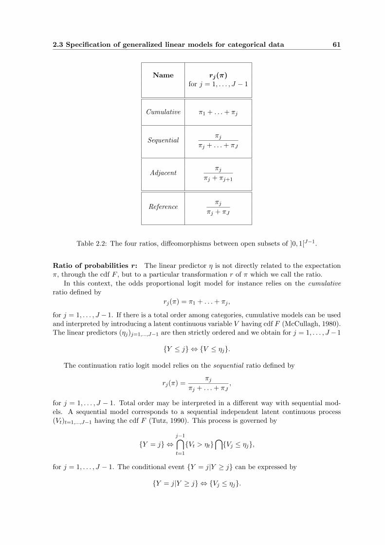
2.3 Specification of generalized linear models for categorical data 61
Name rj(π)for j = 1, . . . , J − 1
Cumulative π1 + . . .+ πj
Sequentialπj
πj + . . .+ πJ
Adjacentπj
πj + πj+1
Referenceπj
πj + πJ
Table 2.2: The four ratios, diffeomorphisms between open subsets of ]0, 1[J−1.
Ratio of probabilities r: The linear predictor η is not directly related to the expectationπ, through the cdf F , but to a particular transformation r of π which we call the ratio.
In this context, the odds proportional logit model for instance relies on the cumulativeratio defined by
rj(π) = π1 + . . .+ πj ,
for j = 1, . . . , J − 1. If there is a total order among categories, cumulative models can be usedand interpreted by introducing a latent continuous variable V having cdf F (McCullagh, 1980).The linear predictors (ηj)j=1,...,J−1 are then strictly ordered and we obtain for j = 1, . . . , J −1
Y ≤ j ⇔ V ≤ ηj.
The continuation ratio logit model relies on the sequential ratio defined by
rj(π) =πj
πj + . . .+ πJ,
for j = 1, . . . , J − 1. Total order may be interpreted in a different way with sequential mod-els. A sequential model corresponds to a sequential independent latent continuous process(Vt)t=1,...,J−1 having the cdf F (Tutz, 1990). This process is governed by
Y = j ⇔j−1⋂t=1
Vt > ηt⋂Vj ≤ ηj,
for j = 1, . . . , J − 1. The conditional event Y = j|Y ≥ j can be expressed by
Y = j|Y ≥ j ⇔ Vj ≤ ηj.

62 2. A new specification of generalized linear models for categorical data
The adjacent logit model is based on the adjacent ratio defined by
rj(π) =πj
πj + πj+1,
for j = 1, . . . , J − 1. Adjacent models are not directly interpretable using latent variables.
Unlike these models for ordinal data, we propose to define a ratio that is independent ofthe category ordering assumption. Using the structure of the multinomial logit model, wedefine the reference ratio for each category j = 1, . . . , J − 1 as
rj(π) =πj
πj + πJ.
Each category j is then related to a reference category (here J by convention) and thus nocategory ordering is assumed. Therefore, the reference ratio allows us to define new GLMs fornominal response variables.
Multinomial logit model
P (Y = j) =exp(αj + xT δj)
1 +∑J−1
k=1 exp(αk + xT δk)(reference, logistic, complete)
Odds proportional logit model
ln
P (Y ≤ j)
1− P (Y ≤ j)
= αj + xT δ (cumulative, logistic, proportional)
Proportional hazard model(Grouped Cox Model)
ln − lnP (Y > j|Y ≥ j) = αj + xT δ (sequential, Gumbel min, proportional)
Adjacent logit model
ln
P (Y = j)
P (Y = j + 1)
= αj + xT δj (adjacent, logistic, complete)
Continuation ratio logit model
ln
P (Y = j)
P (Y > j)
= αj + xT δj (sequential, logistic, complete)
Table 2.3: (r, F, Z) specification of five classical GLMs for categorical data.
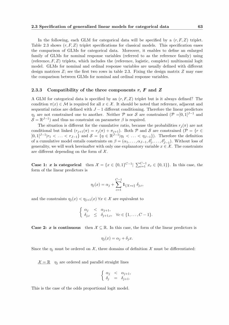
2.3 Specification of generalized linear models for categorical data 63
In the following, each GLM for categorical data will be specified by a (r, F, Z) triplet.Table 2.3 shows (r, F, Z) triplet specifications for classical models. This specification easesthe comparison of GLMs for categorical data. Moreover, it enables to define an enlargedfamily of GLMs for nominal response variables (referred to as the reference family) using(reference, F, Z) triplets, which includes the (reference, logistic, complete) multinomial logitmodel. GLMs for nominal and ordinal response variables are usually defined with differentdesign matrices Z; see the first two rows in table 2.3. Fixing the design matrix Z may easethe comparison between GLMs for nominal and ordinal response variables.
2.3.3 Compatibility of the three components r, F and Z
A GLM for categorical data is specified by an (r, F, Z) triplet but is it always defined? Thecondition π(x) ∈M is required for all x ∈ X . It should be noted that reference, adjacent andsequential ratios are defined with J − 1 different conditioning. Therefore the linear predictorsηj are not constrained one to another. Neither P nor S are constrained (P =]0, 1[J−1 andS = RJ−1) and thus no constraint on parameter β is required.
The situation is different for the cumulative ratio, because the probabilities rj(π) are notconditional but linked (rj+1(π) = rj(π) + πj+1). Both P and S are constrained (P = r ∈]0, 1[J−1|r1 < . . . < rJ−1 and S = η ∈ RJ−1|η1 < . . . < ηJ−1). Therefore the definitionof a cumulative model entails constraints on β = (α1, . . . , αJ−1, δ
t1, . . . , δ
tJ−1). Without loss of
generality, we will work hereinafter with only one explanatory variable x ∈ X . The constraintsare different depending on the form of X .
Case 1: x is categorical then X = x ∈ 0, 1C−1|∑C−1
c=1 xc ∈ 0, 1. In this case, theform of the linear predictors is
ηj(x) = αj +C−1∑c=1
1X=c δj,c,
and the constraints ηj(x) < ηj+1(x) ∀x ∈ X are equivalent toαj < αj+1,δj,c ≤ δj+1,c, ∀c ∈ 1, . . . , C − 1.
Case 2: x is continuous then X ⊆ R. In this case, the form of the linear predictors is
ηj(x) = αj + δjx.
Since the ηj must be ordered on X , three domains of definition X must be differentiated:
X = R ηj are ordered and parallel straight linesαj < αj+1,δj = δj+1.
This is the case of the odds proportional logit model.

64 2. A new specification of generalized linear models for categorical data
X = R+ ηj are ordered and non-intersected half-linesαj < αj+1,δj ≤ δj+1.
This is the case of a positive continuous variable X, such as a size or a dosage for instance.Moreover, if X is strictly positive, the intercepts αj can be common.
X = [a, b] ηj are ordered and non-intersected segments. The constraints cannot be simplyrewritten in terms of intercept and slope constraints.
Figure 2.1: Linear predictors for different configurations of the continuous space X .
For the last two cases a vector of probabilities π(x) for x out of X cannot always bepredicted (see figure 2.1).
2.3.4 Fisher’s scoring algorithm
For maximum likelihood estimation, the iteration of Fisher’s scoring algorithm is given by
β[t+1] = β[t] −
E
(∂2l
∂βT∂β
)β=β[t]
−1(∂l
∂β
)β=β[t]
.
For the sake of simplicity, the algorithm is detailed for only one observation (y, x) with l =lnP (Y = y|X = x;β). Using the chain rule we obtain the score
∂l
∂β=∂η
∂β
∂π
∂η
∂θ
∂π
∂l
∂θ.
Using Property 5, we obtain
∂l
∂β= Zt
∂π
∂ηCov(Y |x)−1 [y − π].
Then using decomposition (3.1) of the link function we obtain
∂l
∂β= Zt
∂F∂η
∂π
∂rCov(Y |x)−1 [y − π]. (2.2)
2.4 Properties of GLMs for categorical data 65
Again using Property 5 and decomposition (3.1) of the link function, we obtain Fisher’s infor-mation matrix
E
(∂2l
∂βt∂β
)= −∂π
∂βCov(Y |x)−1 ∂π
∂βt
= −Zt ∂π∂η
Cov(Y |x)−1 ∂π
∂ηtZ
E
(∂2l
∂βt∂β
)= −Zt ∂F
∂η
∂π
∂rCov(Y |x)−1 ∂π
∂rt∂F∂ηt
Z. (2.3)
We only need to evaluate the associated density function f(ηj)j=1,...,J−1 to compute thediagonal Jacobian matrix ∂F/∂η. For details on computation of the Jacobian matrix ∂π/∂raccording to each ratio, see appendix B.
2.4 Properties of GLMs for categorical data
This section focuses on equivalences between GLMs for categorical data. All the followingproperties strongly depend on the link function, especially the ratio. It should be noted thatfor the case J = 2, all four ratios (see table 2.2) are the same, leading to the Bernoulli case.Hence we focus only on the case J > 2.
The truncated multinomial distribution TM(π) is fully specified by parameter π of dimen-sion J − 1. Therefore, the distribution of Y |X = x is fully specified by the (r, F, Z) triplet fora fixed value of β ∈ C
π = r−1 FZ(x)β.
Equality and equivalence between two models are differentiated here, using the (r, F, Z) spec-ification.
Remark 1. In this thesis we employ model when the three component r, F and Z are de-termined, whereas we employ family of models when at least one of the three components isundetermined. For example (reference, logistic, complete) is a model, whereas (reference, F ,Z)| F ∈ F, Z ∈ Z is a family of models.
Definition 4. Two models (r, F, Z) and (r′, F ′, Z ′) are said to be equal if the correspondingdistributions of Y |X = x are equal for all x and all β
r−1 FZ(x)β = r′−1 F ′Z ′(x)β, ∀x ∈ X , ∀β ∈ C.
Definition 5. Two models (r, F, Z) and (r′, F ′, Z ′) are said to be equivalent if one is areparametrization of the other, and conversely. Hence, there exists a bijection h from C to C′such that
r−1 FZ(x)β = r′−1 F ′Z ′(x)h(β), ∀x ∈ X , ∀β ∈ C.
It should be noted that equality between two models necessarily means that they are alsoequivalent.
2.4.1 Equivalence between GLMs for categorical data
In this subsection we first compare sequential and cumulative ratios, both of which are usedfor ordinal data, then compare reference and adjacent ratios, used for nominal and ordinaldata, respectively.

66 2. A new specification of generalized linear models for categorical data
2.4.1.1 Comparison between sequential and cumulative models
We first remind two equivalences between models for ordinal response variables and extend thesecond one for other design matrices. Thus, we obtain equality between families of sequentialand cumulative models using a transformation between design matrices. Finally, we focus onparticular models for the complete and proportional design matrices.
Equivalences between models Laara and Matthews (1985) showed the equivalence be-tween (sequential, Gumbel min, proportional) and (cumulative, Gumbel min, proportional)models. Tutz (1991) noted that “equivalence holds only for the simple version of the modelswhere the thresholds are not determined by the explanatory variables”. In our framework,this means that (sequential, Gumbel min, Z) and (cumulative, Gumbel min, Z) models areequivalent only for the proportional design matrix Zp. Consider the bijection between the twopredictor spaces S = RJ−1 and S ′ = η ∈ RJ−1|η1 < . . . < ηJ−1 for j = 1, . . . , J − 1 definedby
η′j = ln
j∑
k=1
exp(ηk)
,
which is not linear with respect to η. The predictor η′ must be linear at least with respect tox. Rewriting η′j as
η′j = ln
j∑
k=1
exp(αk) exp(xtδk)
,
we see that linearity with respect to x holds if and only if δ1 = . . . = δJ−1. This corresponds tothe proportional design matrix. Finally the equivalence of Laara and Matthews (1985) holdswith the bijection h between C = RJ−1+p and C′ = β ∈ RJ−1+p|α1 < . . . < αJ−1 defined by α′j = ln
j∑
k=1
exp(αk)
, for j = 1, . . . , J − 1,
δ′ = δ.
The equivalence shown by Tutz (1991)
(cumulative, exponential, complete)⇔ (sequential, exponential, complete),
is quite different because the reparametrization is linear with respect to η. This result cantherefore be generalized for any design matrix.
Equality between families of models It should be noted that the exponential cdf isdefined only for strictly positive values. Therefore, the following property holds only forparameter values β such that η = Zβ ∈ R∗J−1
+ .
Property 6. The two families of models (cumulative, exponential, Z); Z ∈ Z and (sequential,exponential, Z); Z ∈ Z are equal.
Proof. The equality between the two families is shown using double inclusion method. Assumethat the distribution of Y |X = x is defined by the (cumulative, exponential, Z) model withan unknown design matrix Z ∈ Z. For j = 1, . . . , J − 1 we obtain
π1 + . . .+ πj = 1− exp(−ηj). (2.4)

2.4 Properties of GLMs for categorical data 67
The sequential ratio can be rewritten in terms of cumulative ratio
πjπj + . . .+ πJ
=(π1 + . . .+ πj)− (π1 + . . .+ πj−1)
1− (π1 + . . .+ πj−1),
for j = 2, . . . , J − 1. Using (2.4) it becomes
πjπj + . . .+ πJ
= 1− exp−(ηj − ηj−1),
for j = 2, . . . , J − 1. Therefore, we consider the reparametrizationη′1 = η1,η′j = ηj − ηj−1 for j = 2, . . . , J − 1,
between the two predictor spaces S = η ∈ RJ−1|0 ≤ η1 < . . . < ηJ−1 and S ′ = R∗J−1+ . As
this transformation is linear with respect to η, we introduce the following square matrix
A =
1−1 1
. . .. . .
−1 1
of dimension J − 1 and then
η′ = Aη,
η′ = AZβ.
Hence Y |X = x follows the (sequential, exponential, AZ) model with the same parameter β.This means that
(cumulative, exponential, Z) = (sequential, exponential, AZ),
and we thus obtain first inclusion. Finally, noting that A is invertible we obtain
(cumulative, exponential, A−1Z) = (sequential, exponential, Z),
and we thus obtain second inclusion.
Proportional and complete design matrices It should be remarked that A changes ingeneral the constraints on space C and thus the likelihood maximum. For example, the designmatrix Zp corresponds to the constrained space C = β ∈ R(J−1)(1+p)|δ1 = . . . = δJ−1,whereas the design matrix
AZp =
1 xt
−1 1 0. . .
. . ....
−1 1 0
corresponds to the constrained space C = β ∈ R(J−1)(1+p)|δ2 = . . . = δJ−1 = 0. Thedesign matrices Zp and AZp are not equivalent and thus the (cumulative, exponential, Zp) and(sequential, exponential, Zp) models are not equivalent, whereas the (cumulative, exponential,

68 2. A new specification of generalized linear models for categorical data
Zp) and (sequential, exponential, AZp) models are equal. In the same way, the (cumulative,exponential, A−1Zp) and (sequential, exponential, Zp) models are equal with
A−1Zp =
1 xt
1 1 2xt
.... . .
...1 1 . . . 1 (J − 1)xt
.
For the particular complete design there is no constraint on C, thus A cannot change it.We must simply check that A does not reduce the dimension of C. Since A has full rank,the matrices Zc and AZc are equivalent. Therefore the equality between the (cumulative,exponential, Zc) and (sequential, exponential, AZc) models becomes
(cumulative, exponential, Zc)⇔ (sequential, exponential, Zc),
and we recover the equivalence described by Tutz (1991).
Comparison between reference and adjacent models
Here we follow the same approach as previously with sequential and cumulative ratios, andthus provide fewer details. We start from the equivalence
(reference, logistic, complete)⇔ (adjacent, logistic, complete), (2.5)
shown by Agresti (2010) and then generalize this equivalence for any design matrix. Beforestarting, the family of canonical models must be introduced using the (r, F, Z) specification.In the GLM framework, a model is said to be canonical if the equality between the naturalparameter θ and the linear predictor η holds. This equality can be rewritten in terms of linkfunction g = F−1 r.
θ = η
⇔ ln
(πjπJ
)= ηj ∀j = 1, . . . , J − 1
⇔ πjπj + πJ
=exp(ηj)
1 + exp(ηj)∀j = 1, . . . , J − 1.
The reference ratio r can be recognized on the left hand side and the logistic cdf F on theright hand side. Therefore, the family of canonical models is (reference, logistic, Z); Z ∈ Z.The multinomial logit model is a particular canonical model with the complete design matrix.Finally, we generalize the equivalence, described by Agresti (2010), between two models to thefamily of canonical models.
Property 7. The family of canonical models (reference, logistic, Z); Z ∈ Z is equal to thefamily of models (adjacent, logistic, Z); Z ∈ Z.
Proof. Following the same approach as for Property 6 proof, we can see that (reference, logistic,Z) and (adjacent, logistic, AtZ) models are equal for every design matrix Z ∈ Z, where At
turns out to be the transpose of the matrix A previously defined. Noting that At is invertible((At)−1 = (A−1)t), we obtain the desired result.
As previously, At generally changes the constraints on space C. For example, the designmatrices Zp and AtZp are not equivalent. The particular equality
(reference, logistic, (A−1)tZp) = (adjacent, logistic, Zp),
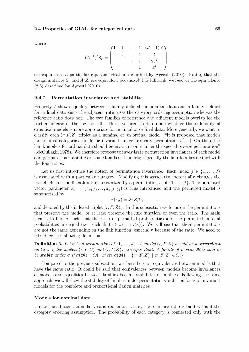
2.4 Properties of GLMs for categorical data 69
where
(A−1)tZp =
1 1 . . . 1 (J − 1)xt
. . ....
...1 1 2xt
1 xt
,
corresponds to a particular reparametrization described by Agresti (2010). Noting that thedesign matrices Zc and AtZc are equivalent because At has full rank, we recover the equivalence(2.5) described by Agresti (2010).
2.4.2 Permutation invariance and stability
Property 7 shows equality between a family defined for nominal data and a family definedfor ordinal data since the adjacent ratio uses the category ordering assumption whereas thereference ratio does not. The two families of reference and adjacent models overlap for theparticular case of the logistic cdf. Thus, we need to determine whether this subfamily ofcanonical models is more appropriate for nominal or ordinal data. More generally, we want toclassify each (r, F, Z) triplet as a nominal or an ordinal model. “It is proposed that modelsfor nominal categories should be invariant under arbitrary permutations [. . . ] On the otherhand, models for ordinal data should be invariant only under the special reverse permutation”(McCullagh, 1978). We therefore propose to investigate permutation invariances of each modeland permutation stabilities of some families of models; especially the four families defined withthe four ratios.
Let us first introduce the notion of permutation invariance. Each index j ∈ 1, . . . , Jis associated with a particular category. Modifying this association potentially changes themodel. Such a modification is characterized by a permutation σ of 1, . . . , J. The permutedvector parameter πσ = (πσ(1), . . . , πσ(J−1)) is thus introduced and the permuted model issummarized by
r(πσ) = F(Zβ),
and denoted by the indexed triplet (r, F, Z)σ. In this subsection we focus on the permutationsthat preserve the model, or at least preserve the link function, or even the ratio. The mainidea is to find σ such that the ratio of permuted probabilities and the permuted ratio ofprobabilities are equal (i.e. such that r(πσ) = rσ(π)). We will see that these permutationsare not the same depending on the link function, especially because of the ratio. We need tointroduce the following definition.
Definition 6. Let σ be a permutation of 1, . . . , J. A model (r, F, Z) is said to be invariantunder σ if the models (r, F, Z) and (r, F, Z)σ are equivalent. A family of models M is said tobe stable under σ if σ(M) = M, where σ(M) = (r, F, Z)σ| (r, F, Z) ∈M.
Compared to the previous subsection, we focus here on equivalences between models thathave the same ratio. It could be said that equivalences between models become invariancesof models and equalities between families become stabilities of families. Following the sameapproach, we will show the stability of families under permutations and then focus on invariantmodels for the complete and proportional design matrices.
Models for nominal data
Unlike the adjacent, cumulative and sequential ratios, the reference ratio is built without thecategory ordering assumption. The probability of each category is connected only with the
70 2. A new specification of generalized linear models for categorical data
probability of reference category J . Thus, changing the reference category could change thefit. Contrary to all the other permutations we have the following property.
Property 8. The family of models (reference, F , Z); F ∈ F, Z ∈ Z is stable under the(J − 1)! permutations that fix the reference category.
Proof. Let σ denote a permutation of 1, . . . , J such that σ(J) = J . For the reference ratioit can be shown that
rj(πσ) = rσ(j)(π),
for j ∈ 1, . . . , J − 1. Thus we need to permute the linear predictors ηj using the restrictedpermutation matrix of dimension J − 1, defined as follows
(Pσ)i,j =
1 if i = σ(j),0 otherwise,
for i, j ∈ 1, . . . , J − 1. Noting that η′ = Pση = PσZβ we obtain
(reference, F, Z)σ = (reference, F, PσZ),
for all F ∈ F and all Z ∈ Z. Noting that Pσ is invertible (P−1σ = Pσ−1) we obtain the desired
result.
Furthermore, the design matrices Zc and PσZc are equivalent because Pσ has full rank.Therefore, (reference, F , Zc)σ and (reference, F , Zc) models are equivalent, which means that(reference, F , Zc) model is invariant under σ. Moreover, the design matrices Zp and PσZp arealso equivalent. In fact, permutation σ does not change the contrast of common slope
δ1 = . . . = δJ−1 ⇔ δσ(1) = . . . = δσ(J−1).
Finally, noting that Zc and PσZc (respectively Zp and PσZp) are equivalent, we obtain thefollowing property of invariance.
Property 9. Let F ∈ F. The two (reference, F , complete) and (reference, F , proportional)models are invariant under the (J − 1)! permutations that fix the reference category.
But what happens if we transpose the reference category? The family of canonical modelshas the following property.
Property 10. The family of canonical models (reference, logistic, Z); Z ∈ Z is stable underall permutations.
Proof. Let τ denote a non identical transposition of the reference category J . Using Property8, we need to show stability under τ . Assume that the distribution of Y |X = x is defined bythe transposed canonical (reference, logistic, Z)τ model. Thus we obtain
πjπτ(J)
= exp(ηj) for j 6= J and j 6= τ(J),
πJπτ(J)
= exp(ητ(J)),
or equivalentlyπjπJ
=πjπτ(J)
πτ(J)
πJ= exp(ηj − ητ(J)) forj 6= J and j 6= τ(J),
πτ(J)
πJ= exp(−ητ(J)).
2.4 Properties of GLMs for categorical data 71
Hence Y |X = x follows the canonical (reference, logistic, BτZ) model, where Bτ is the (J−1)-identity matrix, whose τ(J)th column is replaced by a column of −1. Noting that Bτ isinvertible (B−1
τ = Bτ ) we obtain the desired result.
It should be remarked that the design matrices Zp and BτZp are not equivalent. In factthe contrast δ1 = . . . = δJ−1 becomes δj = 0 for all j 6= τ(J). Thus the (reference, logistic,proportional) model is not invariant under τ but preserves its link function. By contrast, thecanonical (reference, logistic, complete) model is invariant under all permutations because Pσand Bτ have full rank. This last result is just another way of saying that for the multinomiallogit model, the choice of the reference category has no impact on model’s fit. This holds onlyfor this model and its adjacent equivalent. Finally, the (adjacent, logistic, complete) model,which is invariant under all permutations, is inappropriate for ordinal data. More generally,the family of models (adjacent, logistic, Z); Z ∈ Z, which is stable under all permutations(properties 7 and 10), is inappropriate for ordinal data.
Models for ordinal data
Adjacent, cumulative and sequential ratios are defined with the category ordering assumptionand thus are naturally devoted to ordinal data. We therefore expect a permutation whichchanges the order to change also the corresponding models. But what happens if we simplyreverse the order? We would like the model to be invariant. McCullagh (1980) noted thatthe three models (cumulative, logistic, proportional), (cumulative, normal, proportional) and(cumulative, Cauchy, proportional) are invariant under the reverse permutation. More gener-ally, we demonstrate stability of the cumulative family of models under this permutation. Theadjacent ratio turns out to have the same property, unlike the sequential ratio.
Property 11. The two families of models (adjacent, F , Z); F ∈ F, Z ∈ Z and (cumulative,F , Z); F ∈ F, Z ∈ Z are stable under the reverse permutation.
Proof. Let σ denote the reverse permutation (i.e. σ(j) = J − j + 1, ∀j ∈ 1, . . . , J − 1). Foradjacent and cumulative ratios, it can be shown that
rj(πσ) = 1− rJ−j(π), (2.6)
for j ∈ 1, . . . , J − 1. Assume that the distribution Y |X = x is defined by the permuted(r, F, Z)σ model with r = adjacent or cumulative, i.e.
rj(πσ) = F (ηj),
for j ∈ 1, . . . , J − 1. Using equality (2.6), we obtain equivalently
rJ−j(π) = F (−ηj), (2.7)
for j ∈ 1, . . . , J − 1. Now we denote i = J − j and (2.7) becomes
ri(π) = F (−ηJ−i),
for i ∈ 1, . . . , J−1. Hence Y |X = x follows the (r, F ,−PZ) model, where P is the restrictedreverse permutation matrix of dimension J − 1
P =
1. .
.
1
.
72 2. A new specification of generalized linear models for categorical data
Finally we have(adjacent, F,Z) = (adjacent, F ,−PZ),
and(cumulative, F,Z) = (cumulative, F ,−PZ).
Noting that P is invertible (P−1 = P ) we obtain the desired result.
The design matrices Zp and −PZp are equivalent because
δ1 = . . . = δJ−1 ⇔ −δJ = . . . = −δ1.
The design matrices Zc and −PZc are also equivalent because P has full rank. Finally, weobtain the following property of invariance.
Property 12. Let F ∈ F. The four (adjacent, F , complete), (adjacent, F , proportional),(cumulative, F , complete) and (cumulative, F , proportional) models are invariant under thereverse permutation.
For example, the (cumulative, Laplace, proportional) model is invariant under the reversepermutation, whereas the (cumulative, Gumbel min, proportional) model is not. But the(cumulative, Gumbel min, proportional)σ and (cumulative, Gumbel max, proportional) modelsare equivalent.
The situation is quite different for sequential models because equality (2.6) is no longervalid. The reverse permutation changes the structure of a sequential model. Using the equiv-alence between sequential and cumulative models shown by Laara and Matthews (1985), andthe previous result, we obtain the following equivalence under the reverse permutation
(sequential, Gumbel min, proportional)σ ⇔ (cumulative, Gumbel max, proportional).
But for other sequential models, if we introduce the elementary transposition τ of the last twocategories, we obtain the following property.
Property 13. The family of models (sequential, F , Z); F ∈ F, Z ∈ Z is stable under thetransposition τ of the last two categories.
Proof. Assume that the distribution of Y |X = x is defined by the transposed (sequential, F ,Z)τ model with a symmetric cdf F . Thus we obtain
πτ(j)
πτ(j) + . . .+ πτ(J−1) + πτ(J)= F (ηj),
for j ∈ 1, . . . , J − 1. The last equation can be isolatedπj
πj + . . .+ πJ= F (ηj) ∀j ∈ 1, . . . , J − 2,
πJπJ + πJ−1
= F (ηJ−1).
This is equivalent to πj
πj + . . .+ πJ= F (ηj), ∀j ∈ 1, . . . , J − 2,
πJ−1
πJ−1 + πJ= F (−ηJ−1).
2.5 Investigation of invariance properties using benchmark datasets 73
Since F is symmetric (i.e. F = F ), then Y |X = x follows the (sequential, F , AτZ) model,where Aτ is the following squared matrix of dimension J − 1
Aτ =
1
. . .
1−1
.
Noting that Aτ is invertible (A−1τ = Aτ ) we obtain the desired result.
Furthermore, noting that AτZc and Zc are equivalent because Aτ has full rank, we obtainthe following property of invariance:
Property 14. Let F ∈ F. The (sequential, F , complete) model is invariant under the trans-position τ of the last two categories.
However the design matrices AτZ and Z are not equivalent in general. For example, theparticular design matrices AτZp and Zp are not equivalent. Therefore, the (sequential, F ,proportional) model is not invariant under τ , even if F is symmetric.
2.5 Investigation of invariance properties using benchmarkdatasets
Models for ordinal data should be invariant only under the reverse permutation (McCullagh,1980). According to Property 12, we still have to show that (cumulative, F , complete) and(cumulative, F , proportional) models, with F ∈ F, are not invariant under other permutations.But invariance under a permutation is easier to show than the contrary. Thus, we proposed toinvestigate the J ! permutations on a dataset. To highlight the possible equivalences betweenmodels, all the models were ordered according to their log-likelihood value. Each plateau oflog-likelihood therefore likely corresponds to an invariance under a particular permutation.For cumulative models, we thus expect to obtain exactly J !/2! plateaus. If cumulative modelsare invariant under other permutations, we expect some merging of plateaus.
We used the boy’s disturbed dreams benchmark dataset (given in table 2.4) drawn from astudy that cross-classified boys by their age x and the severity of their disturbed dreams y(Maxwell, 1961). The explanatory variable x was assigned mid-point values for each stratumand was used as a continuous variable.
x \ y 1 2 3 4
5-7 7 4 3 78-9 10 15 11 13
10-11 23 9 11 712-13 28 9 12 1014-15 32 5 4 3
Table 2.4: Degree of suffering from disturbed dreams of boys by age.
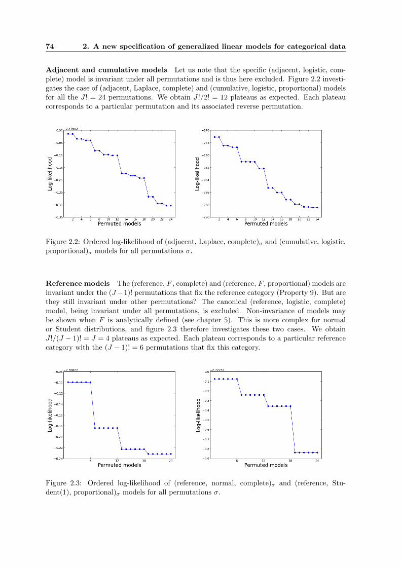
74 2. A new specification of generalized linear models for categorical data
Adjacent and cumulative models Let us note that the specific (adjacent, logistic, com-plete) model is invariant under all permutations and is thus here excluded. Figure 2.2 investi-gates the case of (adjacent, Laplace, complete) and (cumulative, logistic, proportional) modelsfor all the J ! = 24 permutations. We obtain J !/2! = 12 plateaus as expected. Each plateaucorresponds to a particular permutation and its associated reverse permutation.
Figure 2.2: Ordered log-likelihood of (adjacent, Laplace, complete)σ and (cumulative, logistic,proportional)σ models for all permutations σ.
Reference models The (reference, F , complete) and (reference, F , proportional) models areinvariant under the (J−1)! permutations that fix the reference category (Property 9). But arethey still invariant under other permutations? The canonical (reference, logistic, complete)model, being invariant under all permutations, is excluded. Non-invariance of models maybe shown when F is analytically defined (see chapter 5). This is more complex for normalor Student distributions, and figure 2.3 therefore investigates these two cases. We obtainJ !/(J − 1)! = J = 4 plateaus as expected. Each plateau corresponds to a particular referencecategory with the (J − 1)! = 6 permutations that fix this category.
Figure 2.3: Ordered log-likelihood of (reference, normal, complete)σ and (reference, Stu-dent(1), proportional)σ models for all permutations σ.

2.6 Applications 75
Sequential models The (sequential, F , complete) models are invariant under the trans-position of the last two categories when F is symmetric (Property 14). But are they stillinvariant under other permutations? Figure 2.4 investigates the case of (sequential, symmet-ric F , complete) models for all the J ! = 24 permutations, with the logistic and Student(4)cdfs. We obtain J !/2! = 12 plateaus as expected. Each plateau corresponds to a particularpermutation and its associated transposition of the last two categories.
Figure 2.4: Ordered log-likelihood of (sequential, logistic, complete)σ and (sequential, Stu-dent(4), complete)σ models for all permutations σ.
2.6 Applications
2.6.1 Supervised classification
Linear, quadratic and logistic discriminant analyses are three classical methods used for su-pervised classification. The logistic discriminant analysis often outperforms other classicalmethods (Lim et al., 2000). In our context, we prefer to consider the logistic regression ratherthan the logistic discriminant analysis, these two methods being very similar (Hastie et al.,2005). In this subsection, we propose a family of classifiers that includes the logistic regressionas a particular case. We then compare the classification error rates on two benchmark datasets(available on UCI), using 10-fold cross validation. The logistic regression is fully specified bythe (reference, logistic, complete) triplet. This model is more suitable for non-ordered classes,even though it can also be used for ordered classes.
We propose to use the entire set of reference models with a complete design, which haveall the same number of parameters. We can change the cdf F to obtain a better fit. For theapplication, we use ten different cdf F :
F0 = normal, Laplace, Gumbel min, Gumbel max, Student(1), . . . ,Student(6),
from which ten classifiers are built
C∗ = (reference, F, complete); F ∈ F0.
All these classifiers are compared with the logistic regression, using 10-fold cross validation.For each classifier, the mean error rate is computed on the ten sub-samples and compared with
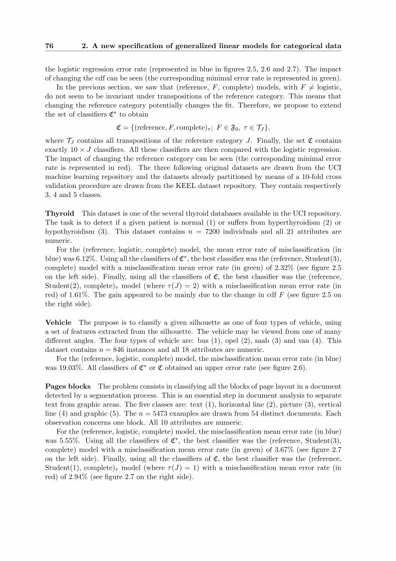
76 2. A new specification of generalized linear models for categorical data
the logistic regression error rate (represented in blue in figures 2.5, 2.6 and 2.7). The impactof changing the cdf can be seen (the corresponding minimal error rate is represented in green).
In the previous section, we saw that (reference, F , complete) models, with F 6= logistic,do not seem to be invariant under transpositions of the reference category. This means thatchanging the reference category potentially changes the fit. Therefore, we propose to extendthe set of classifiers C∗ to obtain
C = (reference, F, complete)τ ; F ∈ F0, τ ∈ TJ,
where TJ contains all transpositions of the reference category J . Finally, the set C containsexactly 10 × J classifiers. All these classifiers are then compared with the logistic regression.The impact of changing the reference category can be seen (the corresponding minimal errorrate is represented in red). The three following original datasets are drawn from the UCImachine learning repository and the datasets already partitioned by means of a 10-fold crossvalidation procedure are drawn from the KEEL dataset repository. They contain respectively3, 4 and 5 classes.
Thyroid This dataset is one of the several thyroid databases available in the UCI repository.The task is to detect if a given patient is normal (1) or suffers from hyperthyroidism (2) orhypothyroidism (3). This dataset contains n = 7200 individuals and all 21 attributes arenumeric.
For the (reference, logistic, complete) model, the mean error rate of misclassification (inblue) was 6.12%. Using all the classifiers of C∗, the best classifier was the (reference, Student(3),complete) model with a misclassification mean error rate (in green) of 2.32% (see figure 2.5on the left side). Finally, using all the classifiers of C, the best classifier was the (reference,Student(2), complete)τ model (where τ(J) = 2) with a misclassification mean error rate (inred) of 1.61%. The gain appeared to be mainly due to the change in cdf F (see figure 2.5 onthe right side).
Vehicle The purpose is to classify a given silhouette as one of four types of vehicle, usinga set of features extracted from the silhouette. The vehicle may be viewed from one of manydifferent angles. The four types of vehicle are: bus (1), opel (2), saab (3) and van (4). Thisdataset contains n = 846 instances and all 18 attributes are numeric.
For the (reference, logistic, complete) model, the misclassification mean error rate (in blue)was 19.03%. All classifiers of C∗ or C obtained an upper error rate (see figure 2.6).
Pages blocks The problem consists in classifying all the blocks of page layout in a documentdetected by a segmentation process. This is an essential step in document analysis to separatetext from graphic areas. The five classes are: text (1), horizontal line (2), picture (3), verticalline (4) and graphic (5). The n = 5473 examples are drawn from 54 distinct documents. Eachobservation concerns one block. All 10 attributes are numeric.
For the (reference, logistic, complete) model, the misclassification mean error rate (in blue)was 5.55%. Using all the classifiers of C∗, the best classifier was the (reference, Student(3),complete) model with a misclassification mean error rate (in green) of 3.67% (see figure 2.7on the left side). Finally, using all the classifiers of C, the best classifier was the (reference,Student(1), complete)τ model (where τ(J) = 1) with a misclassification mean error rate (inred) of 2.94% (see figure 2.7 on the right side).
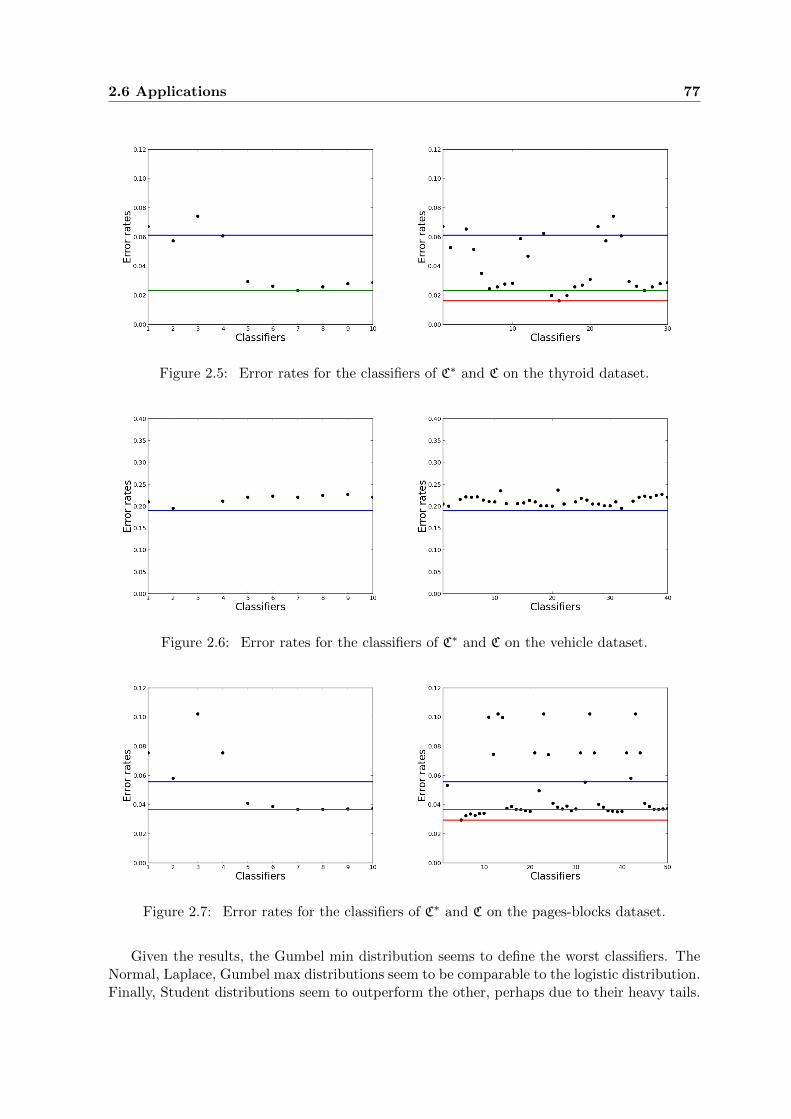
2.6 Applications 77
Figure 2.5: Error rates for the classifiers of C∗ and C on the thyroid dataset.
Figure 2.6: Error rates for the classifiers of C∗ and C on the vehicle dataset.
Figure 2.7: Error rates for the classifiers of C∗ and C on the pages-blocks dataset.
Given the results, the Gumbel min distribution seems to define the worst classifiers. TheNormal, Laplace, Gumbel max distributions seem to be comparable to the logistic distribution.Finally, Student distributions seem to outperform the other, perhaps due to their heavy tails.
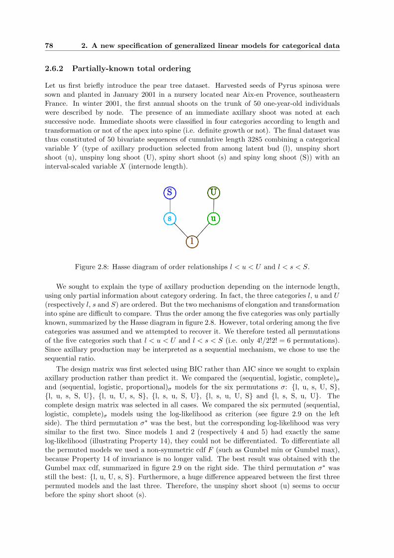
78 2. A new specification of generalized linear models for categorical data
2.6.2 Partially-known total ordering
Let us first briefly introduce the pear tree dataset. Harvested seeds of Pyrus spinosa weresown and planted in January 2001 in a nursery located near Aix-en Provence, southeasternFrance. In winter 2001, the first annual shoots on the trunk of 50 one-year-old individualswere described by node. The presence of an immediate axillary shoot was noted at eachsuccessive node. Immediate shoots were classified in four categories according to length andtransformation or not of the apex into spine (i.e. definite growth or not). The final dataset wasthus constituted of 50 bivariate sequences of cumulative length 3285 combining a categoricalvariable Y (type of axillary production selected from among latent bud (l), unspiny shortshoot (u), unspiny long shoot (U), spiny short shoot (s) and spiny long shoot (S)) with aninterval-scaled variable X (internode length).
Figure 2.8: Hasse diagram of order relationships l < u < U and l < s < S.
We sought to explain the type of axillary production depending on the internode length,using only partial information about category ordering. In fact, the three categories l, u and U(respectively l, s and S) are ordered. But the two mechanisms of elongation and transformationinto spine are difficult to compare. Thus the order among the five categories was only partiallyknown, summarized by the Hasse diagram in figure 2.8. However, total ordering among the fivecategories was assumed and we attempted to recover it. We therefore tested all permutationsof the five categories such that l < u < U and l < s < S (i.e. only 4!/2!2! = 6 permutations).Since axillary production may be interpreted as a sequential mechanism, we chose to use thesequential ratio.
The design matrix was first selected using BIC rather than AIC since we sought to explainaxillary production rather than predict it. We compared the (sequential, logistic, complete)σand (sequential, logistic, proportional)σ models for the six permutations σ: l, u, s, U, S,l, u, s, S, U, l, u, U, s, S, l, s, u, S, U, l, s, u, U, S and l, s, S, u, U. Thecomplete design matrix was selected in all cases. We compared the six permuted (sequential,logistic, complete)σ models using the log-likelihood as criterion (see figure 2.9 on the leftside). The third permutation σ∗ was the best, but the corresponding log-likelihood was verysimilar to the first two. Since models 1 and 2 (respectively 4 and 5) had exactly the samelog-likelihood (illustrating Property 14), they could not be differentiated. To differentiate allthe permuted models we used a non-symmetric cdf F (such as Gumbel min or Gumbel max),because Property 14 of invariance is no longer valid. The best result was obtained with theGumbel max cdf, summarized in figure 2.9 on the right side. The third permutation σ∗ wasstill the best: l, u, U, s, S. Furthermore, a huge difference appeared between the first threepermuted models and the last three. Therefore, the unspiny short shoot (u) seems to occurbefore the spiny short shoot (s).
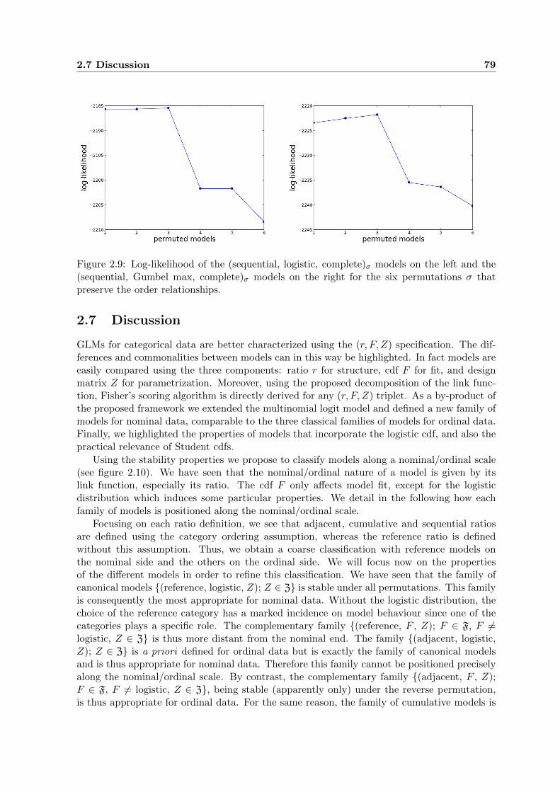
2.7 Discussion 79
Figure 2.9: Log-likelihood of the (sequential, logistic, complete)σ models on the left and the(sequential, Gumbel max, complete)σ models on the right for the six permutations σ thatpreserve the order relationships.
2.7 Discussion
GLMs for categorical data are better characterized using the (r, F, Z) specification. The dif-ferences and commonalities between models can in this way be highlighted. In fact models areeasily compared using the three components: ratio r for structure, cdf F for fit, and designmatrix Z for parametrization. Moreover, using the proposed decomposition of the link func-tion, Fisher’s scoring algorithm is directly derived for any (r, F, Z) triplet. As a by-product ofthe proposed framework we extended the multinomial logit model and defined a new family ofmodels for nominal data, comparable to the three classical families of models for ordinal data.Finally, we highlighted the properties of models that incorporate the logistic cdf, and also thepractical relevance of Student cdfs.
Using the stability properties we propose to classify models along a nominal/ordinal scale(see figure 2.10). We have seen that the nominal/ordinal nature of a model is given by itslink function, especially its ratio. The cdf F only affects model fit, except for the logisticdistribution which induces some particular properties. We detail in the following how eachfamily of models is positioned along the nominal/ordinal scale.
Focusing on each ratio definition, we see that adjacent, cumulative and sequential ratiosare defined using the category ordering assumption, whereas the reference ratio is definedwithout this assumption. Thus, we obtain a coarse classification with reference models onthe nominal side and the others on the ordinal side. We will focus now on the propertiesof the different models in order to refine this classification. We have seen that the family ofcanonical models (reference, logistic, Z); Z ∈ Z is stable under all permutations. This familyis consequently the most appropriate for nominal data. Without the logistic distribution, thechoice of the reference category has a marked incidence on model behaviour since one of thecategories plays a specific role. The complementary family (reference, F , Z); F ∈ F, F 6=logistic, Z ∈ Z is thus more distant from the nominal end. The family (adjacent, logistic,Z); Z ∈ Z is a priori defined for ordinal data but is exactly the family of canonical modelsand is thus appropriate for nominal data. Therefore this family cannot be positioned preciselyalong the nominal/ordinal scale. By contrast, the complementary family (adjacent, F , Z);F ∈ F, F 6= logistic, Z ∈ Z, being stable (apparently only) under the reverse permutation,is thus appropriate for ordinal data. For the same reason, the family of cumulative models is
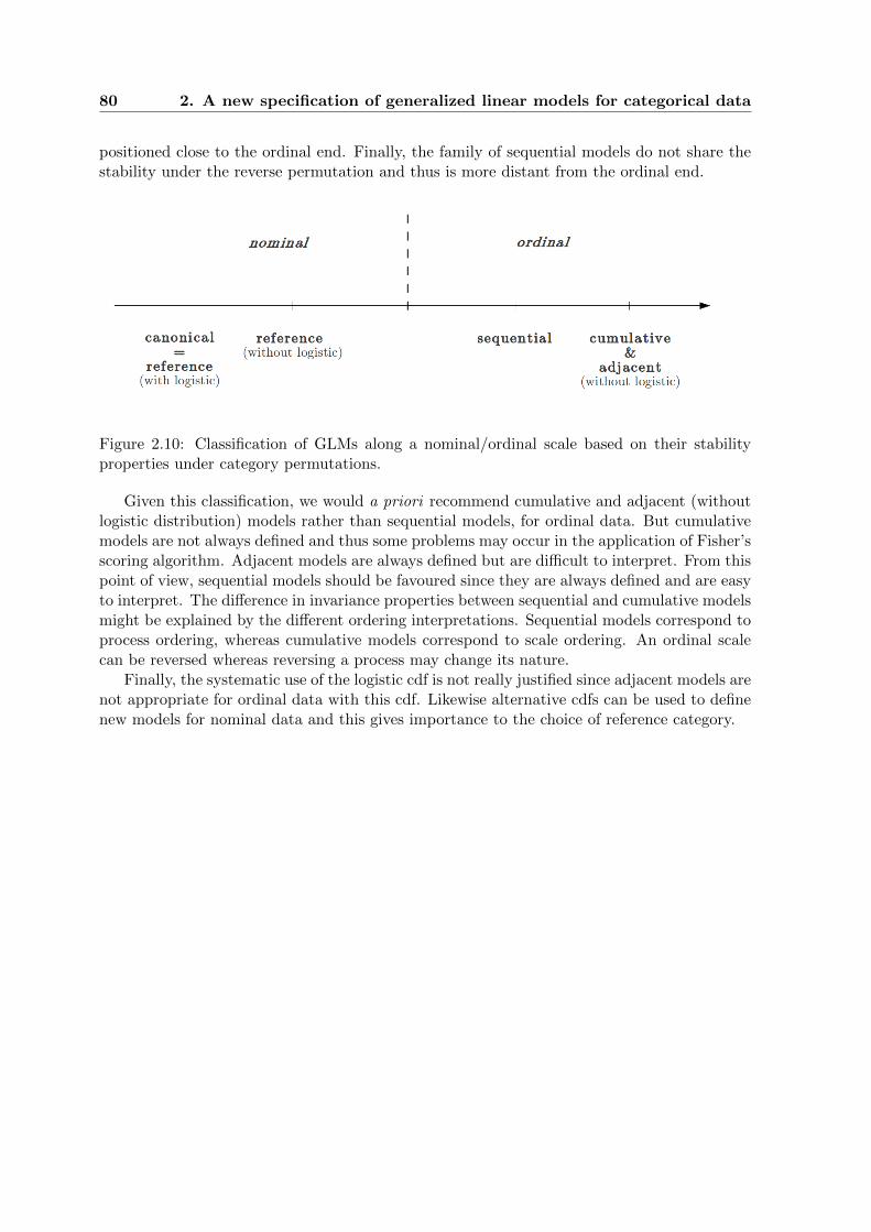
80 2. A new specification of generalized linear models for categorical data
positioned close to the ordinal end. Finally, the family of sequential models do not share thestability under the reverse permutation and thus is more distant from the ordinal end.
Figure 2.10: Classification of GLMs along a nominal/ordinal scale based on their stabilityproperties under category permutations.
Given this classification, we would a priori recommend cumulative and adjacent (withoutlogistic distribution) models rather than sequential models, for ordinal data. But cumulativemodels are not always defined and thus some problems may occur in the application of Fisher’sscoring algorithm. Adjacent models are always defined but are difficult to interpret. From thispoint of view, sequential models should be favoured since they are always defined and are easyto interpret. The difference in invariance properties between sequential and cumulative modelsmight be explained by the different ordering interpretations. Sequential models correspond toprocess ordering, whereas cumulative models correspond to scale ordering. An ordinal scalecan be reversed whereas reversing a process may change its nature.
Finally, the systematic use of the logistic cdf is not really justified since adjacent models arenot appropriate for ordinal data with this cdf. Likewise alternative cdfs can be used to definenew models for nominal data and this gives importance to the choice of reference category.
Chapter 3
Partitioned conditional generalizedlinear models for categorical data
Abstract
In categorical data analysis, several regression models have been proposed for hierarchically-structured response variables, e.g. the nested logit model (McFadden et al., 1978). But theyhave been formally defined for only two or three levels in the hierarchy. Here, we introduce theclass of partitioned conditional generalized linear models (PCGLMs) defined for any numbersof levels. The hierarchical structure of these models is fully specified by a partition tree ofcategories. Using the genericity of the (r, F, Z) specification, the PCGLM can handle nominal,ordinal but also partially-ordered response variables.
Keywords: hierarchically-structured categorical variable, partition tree, nominal variable,ordinal variable, partially-ordered variable, GLM specification.
Contents
3.1 Introduction . . . . . . . . . . . . . . . . . . . . . . . . . . . . . . . . . . 82
3.2 Partitioned conditional GLMs . . . . . . . . . . . . . . . . . . . . . . . . 82
3.2.1 (r,F,Z) specification of GLM for categorical data . . . . . . . . . . . . . . 83
3.2.2 Definition of partitioned conditional GLMs . . . . . . . . . . . . . . . . . 85
3.2.3 Estimation of PCGLMs . . . . . . . . . . . . . . . . . . . . . . . . . . . . 87
3.3 PCGLMs for nominal data . . . . . . . . . . . . . . . . . . . . . . . . . . 88
3.3.1 PCGLM specification of the nested logit model . . . . . . . . . . . . . . . 88
3.3.2 PCGLMs for qualitative choices . . . . . . . . . . . . . . . . . . . . . . . . 90
3.4 PCGLMs for ordinal data . . . . . . . . . . . . . . . . . . . . . . . . . . 90
3.4.1 PCGLM specification of the two-step model . . . . . . . . . . . . . . . . . 90
3.4.2 Indistinguishability of response categories . . . . . . . . . . . . . . . . . . 92
3.5 PCGLMs for partially-ordered data . . . . . . . . . . . . . . . . . . . . 95
3.5.1 PCGLM specification of the POS-PCM . . . . . . . . . . . . . . . . . . . 95
3.5.2 Inference of PCGLMs for partially-ordered data . . . . . . . . . . . . . . . 96
3.6 Applications . . . . . . . . . . . . . . . . . . . . . . . . . . . . . . . . . . 98
3.6.1 Totally ordered data: back pain prognosis example . . . . . . . . . . . . . 98
3.6.2 Partially-ordered data: pear tree example . . . . . . . . . . . . . . . . . . 100
3.7 Discussion . . . . . . . . . . . . . . . . . . . . . . . . . . . . . . . . . . . . 102
82 3. Partitioned conditional generalized linear models for categorical data
3.1 Introduction
Categorical data are often based on a hierarchical structure. Although this may seem natu-ral for partially-ordered or even ordinal data, it still makes sense for nominal data. Severalpartitioned conditional regression models have been proposed in different applied fields, includ-ing econometrics, medicine and psychology. The most well-known is the nested logit model,introduced by McFadden et al. (1978) in econometrics for qualitative choice (i.e. nominalcategories). In the same field, Morawitz and Tutz (1990) introduced the two-step model totake account of hierarchy among ordinal choices. This model is also used in medicine whenordered categories can be decomposed into coarse and fine scales (Tutz, 1989). The partitionedconditional model for partially-ordered set (POS-PCM) was introduced in medicine by Zhangand Ip (2012).
Compared to simple regression models for categorical data, e.g. the multinomial logitand the odds proportional logit models, partitioned conditional models capture several latentmechanisms. The event Y = j is decomposed into several steps corresponding to the latenthierarchical structure, with these steps being potentially influenced by different explanatoryvariables. This approach leads to more flexible models with often a better fit and an easierstep-by-step interpretation. In this chapter we introduce the directed trees as the main toolused to formalize the hierarchical structure among categories.
Until now, partitioned conditional models have been formally defined only for two or threelevels in the hierarchy. Furthermore, they all assume that the hierarchical structure amongthe categories is a priori known. Our first contribution is to use directed trees to specify thehierarchical structure. This enables us to define partitioned conditional models for an arbitrarynumber of levels. Moreover, using the genericity of the (r, F, Z) specification (see chapter 2),we develop an extended class of partitioned conditional models for nominal, ordinal but alsopartially-ordered data. Finally, in the case of ordinal data, instead of considering that thehierarchical structure is known a priori, we propose to recover it.
The (r, F, Z) specification of a GLM for categorical data is reviewed in section 3.2, andpartition trees are defined. We use these two main building blocks to define and estimate theclass of partitioned conditional GLMs.
Sections 3.3, 3.4 and 3.5 extend three existing hierarchically-structured models, revisitingthem with the proposed partitioned conditional GLM framework. These three sections focusrespectively on the nested logit model for nominal data, the two-step model for ordinal dataand the POS-PCM for partially-ordered data. Section 3.4 also describes a model selection pro-cedure for ordinal data, derived from the indistinguishability procedure described by Anderson(1984), which selects the partition tree and at the same time the explanatory variables.
This procedure is illustrated in section 3.6 using the back pain prognosis example previouslyanalysed by Anderson (1984). Our methodology for partially-ordered data is then illustratedusing the pear tree example.
3.2 Partitioned conditional GLMs
This section briefly outlines the (r, F, Z) specification of a GLM for categorical data and itsestimation. The partition tree is then defined in order to specify the hierarchical structureamong categories. Finally, we introduce the class of partitioned conditional GLMs and describethe estimation of such models.
3.2 Partitioned conditional GLMs 83
3.2.1 (r,F,Z) specification of GLM for categorical data
The definition of a GLM includes the specification of a link function g which is a diffeomorphismfrom M = π ∈ ]0, 1[J−1|
∑J−1j=1 πj < 1 to an open subset S of RJ−1. This function links the
expectation π = E[Y |X=x] and the linear predictor η = (η1, ..., ηJ−1)t. It also includes theparametrization of the linear predictor η, which can be written as the product of the designmatrix Z (as a function of x) and the vector of parameters β (Fahrmeir and Tutz, 2001). Allthe classical link functions g = (g1, . . . , gJ−1) described in the literature (Agresti, 2002; Tutz,2012), rely on the same structure which we propose to write as
gj = F−1 rj , j = 1, . . . , J − 1. (3.1)
where F is a continuous and strictly increasing cumulative distribution function (cdf) andr = (r1, . . . , rJ−1)t is a diffeomorphism from M to an open subset P of ]0, 1[J−1. Finally,given x, we propose to summarize a GLM for a categorical response variable by the J − 1equations
r(π) = F(Zβ),
where F(η) = (F (η1), . . . , F (ηJ−1))T . In the following, we describe in more detail the compo-nents r, F and Z.
Ratio r of probabilities: The linear predictor η is not directly related to the expectationπ but to a particular transformation r of the vector π which we call the ratio. In the followingwe will consider four particular diffeomorphisms. The adjacent, sequential and cumulativeratios are respectively defined by rj(π) = πj/(πj + πj+1), rj(π) = πj/(πj + . . . + πJ) andrj(π) = π1 + . . . + πj for j = 1, . . . , J − 1. They all include an order assumption amongcategories, corresponding to different motivations. On the other hand the reference ratio,defined by rj(π) = πj/(πj + πJ) for j = 1, . . . , J − 1, is devoted to nominal response variables.
Cumulative distribution function F : The logistic and normal cdfs are the symmetric cdfsmost commonly used, but Laplace and Student cdfs may also be useful. The Gumbel min andGumbel max cdfs are the asymmetric cdfs most commonly used. Playing on the symmetricalor asymmetrical character, and the more or less heavy tails, may markedly improve model fit.In applications, Student distributions are used with small degrees of freedom.
Design matrix Z: Each linear predictor has the form ηj = αj + xtδj and the vector ofparameters is β = (α1, . . . , αJ−1, δ
t1, . . . , δ
tJ−1) ∈ R(J−1)(1+p) where p is the dimension of the
explanatory space X . The model is generally defined without constraint, as this is the case forthe multinomial logit model. However some linear equality constraints, called contrasts, maybe added for instance between different slopes δj . The most common contrast is the equalityof all slopes, as in the odds proportional logit model. The corresponding constrained spaceC = β ∈ R(J−1)(1+p)|δ1 = . . . = δJ−1 may be identified to R(J−1)+p. Finally the contrastspace is represented by a design matrix. For example, the complete design matrix Zc (withoutconstraint) of dimension (J − 1)× (J − 1)(1 + p) has the following form
Zc =
1 xt
. . .. . .
1 xt
.

84 3. Partitioned conditional generalized linear models for categorical data
The proportional design matrix Zp (common slope) of dimension (J − 1)× (J − 1 + p) has thefollowing form:
Zp =
1 xt
. . ....
1 xt
.
Multinomial logit model
P (Y = j) =exp(αj + xT δj)
1 +∑J−1
k=1 exp(αk + xT δk)(reference, logistic, complete)
Odds proportional logit model
log
P (Y ≤ j)
1− P (Y ≤ j)
= αj + xT δ (cumulative, logistic, proportional)
Proportional hazard model(Grouped Cox Model)
− logP (Y > j|Y ≥ j) = exp(αj + xT δ) (sequential, Gumbel min, proportional)
Adjacent logit model
log
P (Y = j)
P (Y = j + 1)
= αj + xT δj (adjacent, logistic, complete)
Table 3.1: (r, F, Z) specification of four classical GLMs for categorical data.
The triplet (r, F, Z) will play a key role in the following since each GLM for categoricaldata will be specified by one of these triplets. Table 3.1 shows the specification of four classicalmodels. This specification eases the comparison of GLMs for categorical response variables.Moreover, it can be used to define an extended set of GLMs for nominal response variables by(reference, F , Z) triplets, which includes the multinomial logit model.
Finally, a single estimation procedure based on Fisher’s scoring algorithm can be appliedto all the GLMs specified by an (r, F, Z) triplet. The score function can be decomposed intotwo parts, where the first, unlike the second, depends on the (r, F, Z) triplet.
∂l
∂β= ZT
∂F∂η
∂π
∂r︸ ︷︷ ︸(r,F,Z) dependent part
Cov(Y |X = x)−1 [y − π]︸ ︷︷ ︸(r,F,Z) independent part
. (3.2)
3.2 Partitioned conditional GLMs 85
We only need to evaluate the associated density function values f(ηj)j=1,...,J−1 to computethe diagonal Jacobian matrix ∂F/∂η. For details on computation of the Jacobian matrix∂π/∂r for each ratio, see appendix B.
3.2.2 Definition of partitioned conditional GLMs
The main idea is to recursively partition the J categories then specify a conditional GLM ateach step. This type of model is therefore referred to as partitioned conditional GLM. Modelsof this class have already been proposed, e.g. the nested logit model (McFadden et al., 1978),the two-step model (Tutz, 1989) and the partitioned conditional model for partially-orderedset (POS-PCM) (Zhang and Ip, 2012). Our proposal can be seen as a generalization of thesethree models that benefits from the genericity of the (r, F, Z) specification. In particular,our objective is not only to propose GLMs for partially-ordered response variables but alsoto differentiate the role of explanatory variables for each partitioning step using differentdesign matrices and different explanatory variables. We are seeking also to formally definethe partitioned conditional GLMs for any number of levels in the hierarchy. Hence we need tointroduce definitions and notations for directed trees.
Definition 7. A directed tree T is said to be a partition tree of 1, . . . , J if
• 1, . . . , J is the root of T,
• sibling vertices constitute a non identical partition of their parent node,
• each singleton j belongs to T.
In the following, V∗ is the set of non-terminal vertices of T and for each v ∈ V∗, Ch(v) =Ωv
1, . . . ,ΩvJv is the set of indexed children of v. The children must be indexed because the
GLMs are not necessarily invariant under permutation of the response categories (see chapter2). Children Ωv
1, . . . ,ΩvJv
are presented from left to right and ΩvJv
is considered as the referencechild by convention. Also, for each vertex v (except the root), Pa(v) denotes the parent of vand An∗(v) denotes the ancestors set of v except the root.
Definition 8. Let J ≥ 2 and 1 ≤ k ≤ J − 1. A k-partitioned conditional GLM ofcategories 1, . . . , J (k-PCGLM) is specified by
• a partition tree T of 1, . . . , J with card(V∗) = k,
• a collection of models C = (rv, F v, Zv(xv)) | v ∈ V∗ for each conditional prob-ability vector πv = (πv1 , . . . , π
vJv−1), where πvj = P (Y ∈ Ωv
j |Y ∈ v;xv) and xv is asub-vector of x associated with vertex v.
With this definition, the probability of each category j is then obtained by
P (Y = j|x) = P (Y = j|Y ∈ Pa(j), xPa(j))∏
v∈An∗(j)
P (Y ∈ v|Y ∈ Pa(v), xPa(v)),
where P (Y ∈ v|Y ∈ Pa(v), xPa(v)) is described by the GLM of C associated with vertex Pa(v).The class of PCGLMs for categorical response variables is the set of k-PCGLMs for 1 ≤
k ≤ J − 1. The boundary cases are classical GLMs. For instance for k = 1 (see figure 3.1on the left), the root is the only non-terminal vertex of T , thus we have a classical GLM forcategories 1, . . . , J. For k = J − 1 (see figure 3.1 on the right), T is a binary tree and
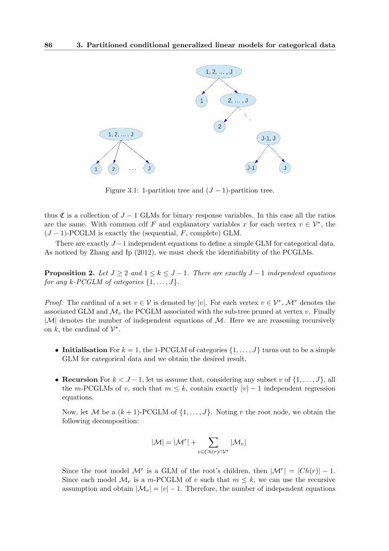
86 3. Partitioned conditional generalized linear models for categorical data
Figure 3.1: 1-partition tree and (J − 1)-partition tree.
thus C is a collection of J − 1 GLMs for binary response variables. In this case all the ratiosare the same. With common cdf F and explanatory variables x for each vertex v ∈ V∗, the(J − 1)-PCGLM is exactly the (sequential, F , complete) GLM.
There are exactly J−1 independent equations to define a simple GLM for categorical data.As noticed by Zhang and Ip (2012), we must check the identifiability of the PCGLMs.
Proposition 2. Let J ≥ 2 and 1 ≤ k ≤ J − 1. There are exactly J − 1 independent equationsfor any k-PCGLM of categories 1, . . . , J.
Proof. The cardinal of a set v ∈ V is denoted by |v|. For each vertex v ∈ V∗, Mv denotes theassociated GLM andMv the PCGLM associated with the sub-tree pruned at vertex v. Finally|M| denotes the number of independent equations of M. Here we are reasoning recursivelyon k, the cardinal of V∗.
• Initialisation For k = 1, the 1-PCGLM of categories 1, . . . , J turns out to be a simpleGLM for categorical data and we obtain the desired result.
• Recursion For k < J − 1, let us assume that, considering any subset v of 1, . . . , J, allthe m-PCGLMs of v, such that m ≤ k, contain exactly |v| − 1 independent regressionequations.
Now, let M be a (k + 1)-PCGLM of 1, . . . , J. Noting r the root node, we obtain thefollowing decomposition:
|M| = |Mr|+∑
v∈Ch(r)∩V∗|Mv|
Since the root model Mr is a GLM of the root’s children, then |Mr| = |Ch(r)| − 1.Since each model Mv is a m-PCGLM of v such that m ≤ k, we can use the recursiveassumption and obtain |Mv| = |v| − 1. Therefore, the number of independent equations
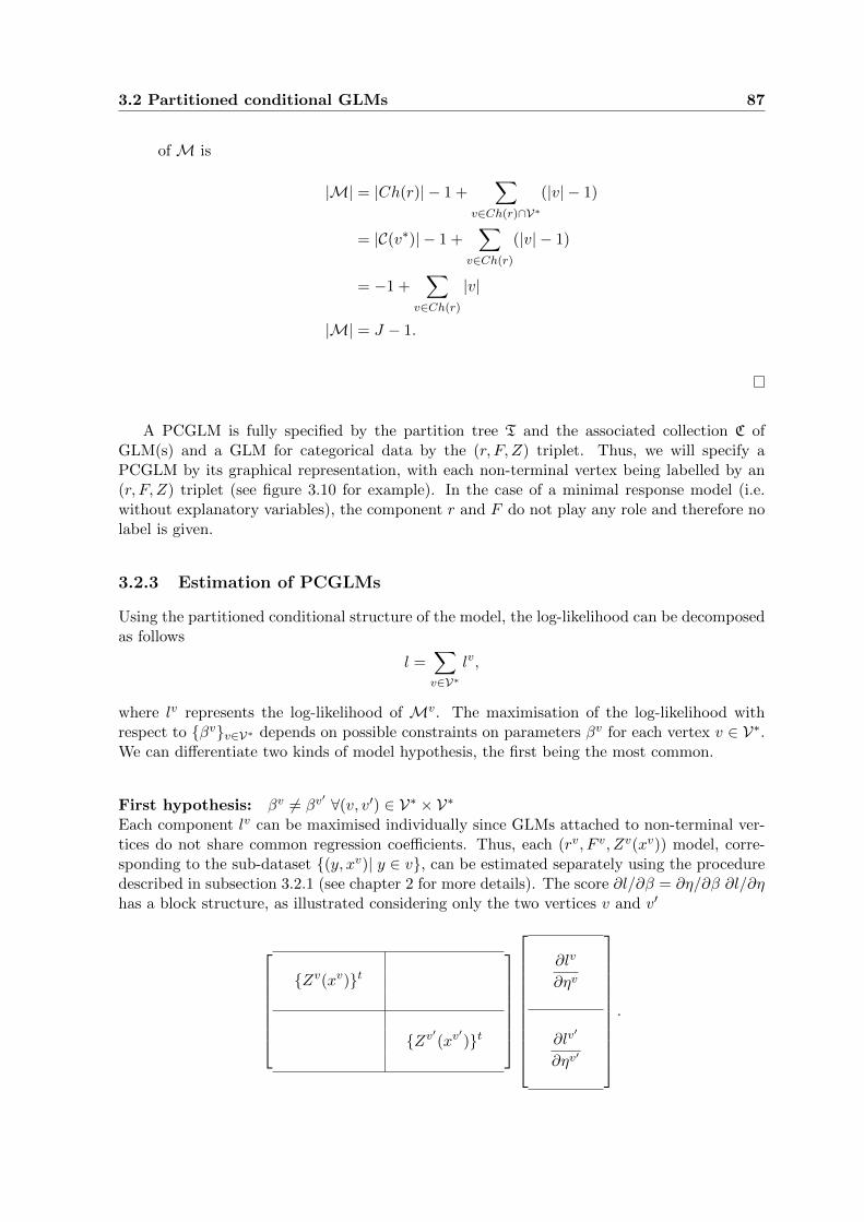
3.2 Partitioned conditional GLMs 87
of M is
|M| = |Ch(r)| − 1 +∑
v∈Ch(r)∩V∗(|v| − 1)
= |C(v∗)| − 1 +∑
v∈Ch(r)
(|v| − 1)
= −1 +∑
v∈Ch(r)
|v|
|M| = J − 1.
A PCGLM is fully specified by the partition tree T and the associated collection C ofGLM(s) and a GLM for categorical data by the (r, F, Z) triplet. Thus, we will specify aPCGLM by its graphical representation, with each non-terminal vertex being labelled by an(r, F, Z) triplet (see figure 3.10 for example). In the case of a minimal response model (i.e.without explanatory variables), the component r and F do not play any role and therefore nolabel is given.
3.2.3 Estimation of PCGLMs
Using the partitioned conditional structure of the model, the log-likelihood can be decomposedas follows
l =∑v∈V∗
lv,
where lv represents the log-likelihood of Mv. The maximisation of the log-likelihood withrespect to βvv∈V∗ depends on possible constraints on parameters βv for each vertex v ∈ V∗.We can differentiate two kinds of model hypothesis, the first being the most common.
First hypothesis: βv 6= βv′ ∀(v, v′) ∈ V∗ × V∗
Each component lv can be maximised individually since GLMs attached to non-terminal ver-tices do not share common regression coefficients. Thus, each (rv, F v, Zv(xv)) model, corre-sponding to the sub-dataset (y, xv)| y ∈ v, can be estimated separately using the proceduredescribed in subsection 3.2.1 (see chapter 2 for more details). The score ∂l/∂β = ∂η/∂β ∂l/∂ηhas a block structure, as illustrated considering only the two vertices v and v′
Zv(xv)t
Zv′(xv′)t
∂lv
∂ηv
∂lv′
∂ηv′
.
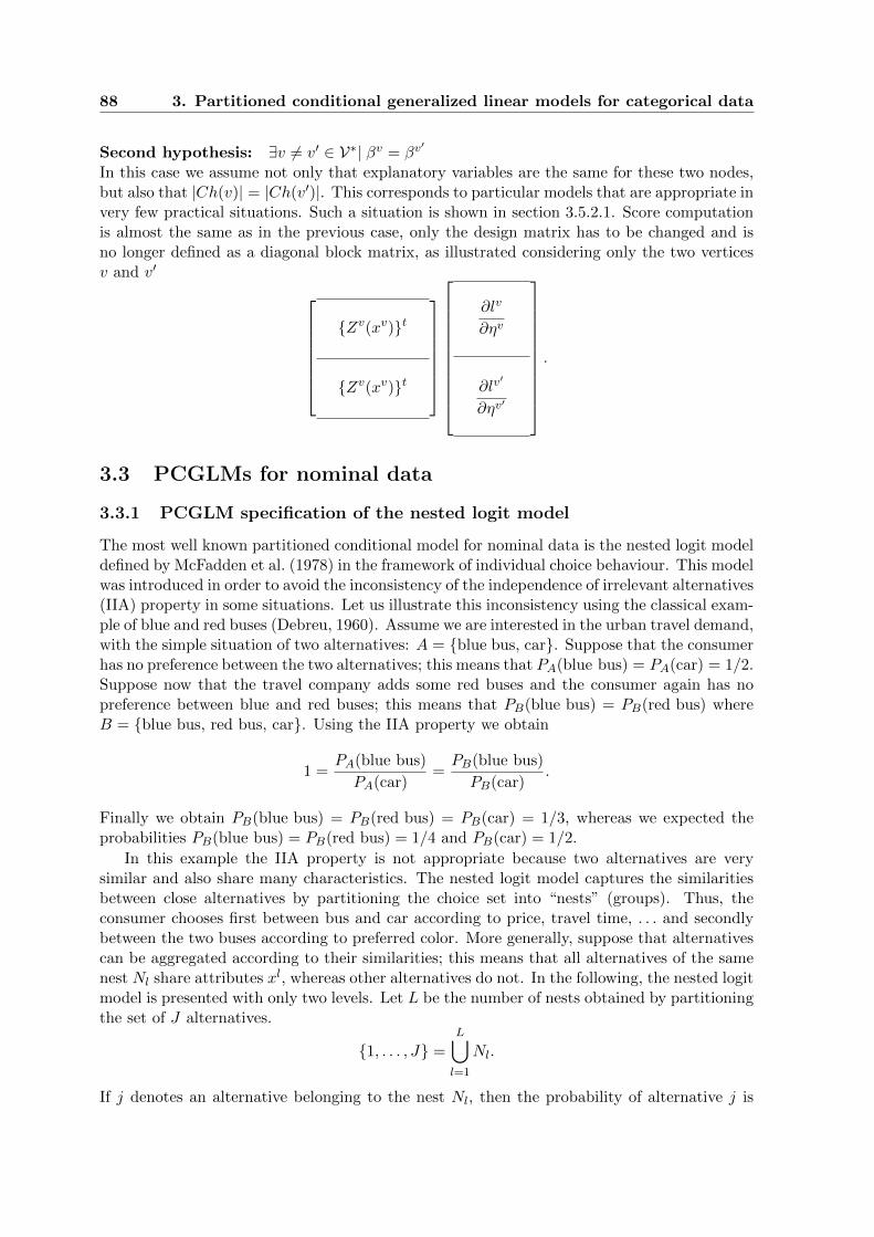
88 3. Partitioned conditional generalized linear models for categorical data
Second hypothesis: ∃v 6= v′ ∈ V∗| βv = βv′
In this case we assume not only that explanatory variables are the same for these two nodes,but also that |Ch(v)| = |Ch(v′)|. This corresponds to particular models that are appropriate invery few practical situations. Such a situation is shown in section 3.5.2.1. Score computationis almost the same as in the previous case, only the design matrix has to be changed and isno longer defined as a diagonal block matrix, as illustrated considering only the two verticesv and v′
Zv(xv)t
Zv(xv)t
∂lv
∂ηv
∂lv′
∂ηv′
.
3.3 PCGLMs for nominal data
3.3.1 PCGLM specification of the nested logit model
The most well known partitioned conditional model for nominal data is the nested logit modeldefined by McFadden et al. (1978) in the framework of individual choice behaviour. This modelwas introduced in order to avoid the inconsistency of the independence of irrelevant alternatives(IIA) property in some situations. Let us illustrate this inconsistency using the classical exam-ple of blue and red buses (Debreu, 1960). Assume we are interested in the urban travel demand,with the simple situation of two alternatives: A = blue bus, car. Suppose that the consumerhas no preference between the two alternatives; this means that PA(blue bus) = PA(car) = 1/2.Suppose now that the travel company adds some red buses and the consumer again has nopreference between blue and red buses; this means that PB(blue bus) = PB(red bus) whereB = blue bus, red bus, car. Using the IIA property we obtain
1 =PA(blue bus)
PA(car)=PB(blue bus)
PB(car).
Finally we obtain PB(blue bus) = PB(red bus) = PB(car) = 1/3, whereas we expected theprobabilities PB(blue bus) = PB(red bus) = 1/4 and PB(car) = 1/2.
In this example the IIA property is not appropriate because two alternatives are verysimilar and also share many characteristics. The nested logit model captures the similaritiesbetween close alternatives by partitioning the choice set into “nests” (groups). Thus, theconsumer chooses first between bus and car according to price, travel time, . . . and secondlybetween the two buses according to preferred color. More generally, suppose that alternativescan be aggregated according to their similarities; this means that all alternatives of the samenest Nl share attributes xl, whereas other alternatives do not. In the following, the nested logitmodel is presented with only two levels. Let L be the number of nests obtained by partitioningthe set of J alternatives.
1, . . . , J =L⋃l=1
Nl.
If j denotes an alternative belonging to the nest Nl, then the probability of alternative j is
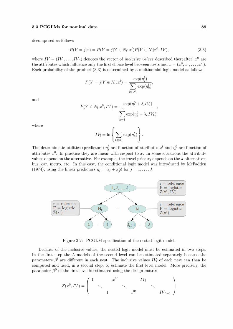
3.3 PCGLMs for nominal data 89
decomposed as follows
P (Y = j|x) = P (Y = j|Y ∈ Nl;xl)P (Y ∈ Nl|x0, IV ), (3.3)
where IV = (IV1, . . . , IVL) denotes the vector of inclusive values described thereafter, x0 arethe attributes which influence only the first choice level between nests and x = (x0, x1, . . . , xL).Each probability of the product (3.3) is determined by a multinomial logit model as follows
P (Y = j|Y ∈ Nl;xl) =
exp(ηlj)∑k∈Nl
exp(ηlk),
and
P (Y ∈ Nl|x0, IV ) =exp(η0
l + λlIVl)L∑k=1
exp(η0k + λkIVk)
,
where
IVl = ln
∑k∈Nl
exp(ηlk)
.
The deterministic utilities (predictors) ηlj are function of attributes xl and η0l are function of
attributes x0. In practice they are linear with respect to x. In some situations the attributevalues depend on the alternative. For example, the travel price xj depends on the J alternativesbus, car, metro, etc. In this case, the conditional logit model was introduced by McFadden(1974), using the linear predictors ηj = αj + xtjδ for j = 1, . . . , J .
Figure 3.2: PCGLM specification of the nested logit model.
Because of the inclusive values, the nested logit model must be estimated in two steps.In the first step the L models of the second level can be estimated separately because theparameters βl are different in each nest. The inclusive values IVl of each nest can then becomputed and used, in a second step, to estimate the first level model. More precisely, theparameter β0 of the first level is estimated using the design matrix
Z(x0, IV ) =
1 x0t IV1
. . .. . .
. . .
1 x0t IVL−1
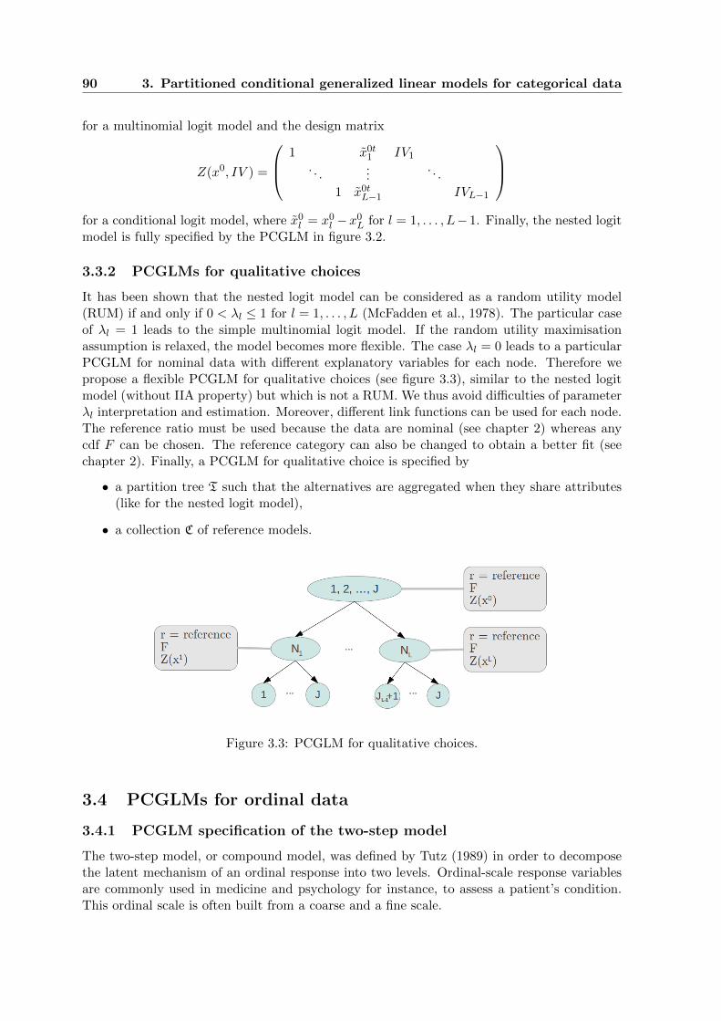
90 3. Partitioned conditional generalized linear models for categorical data
for a multinomial logit model and the design matrix
Z(x0, IV ) =
1 x0t1 IV1
. . ....
. . .
1 x0tL−1 IVL−1
for a conditional logit model, where x0
l = x0l −x0
L for l = 1, . . . , L− 1. Finally, the nested logitmodel is fully specified by the PCGLM in figure 3.2.
3.3.2 PCGLMs for qualitative choices
It has been shown that the nested logit model can be considered as a random utility model(RUM) if and only if 0 < λl ≤ 1 for l = 1, . . . , L (McFadden et al., 1978). The particular caseof λl = 1 leads to the simple multinomial logit model. If the random utility maximisationassumption is relaxed, the model becomes more flexible. The case λl = 0 leads to a particularPCGLM for nominal data with different explanatory variables for each node. Therefore wepropose a flexible PCGLM for qualitative choices (see figure 3.3), similar to the nested logitmodel (without IIA property) but which is not a RUM. We thus avoid difficulties of parameterλl interpretation and estimation. Moreover, different link functions can be used for each node.The reference ratio must be used because the data are nominal (see chapter 2) whereas anycdf F can be chosen. The reference category can also be changed to obtain a better fit (seechapter 2). Finally, a PCGLM for qualitative choice is specified by
• a partition tree T such that the alternatives are aggregated when they share attributes(like for the nested logit model),
• a collection C of reference models.
Figure 3.3: PCGLM for qualitative choices.
3.4 PCGLMs for ordinal data
3.4.1 PCGLM specification of the two-step model
The two-step model, or compound model, was defined by Tutz (1989) in order to decomposethe latent mechanism of an ordinal response into two levels. Ordinal-scale response variablesare commonly used in medicine and psychology for instance, to assess a patient’s condition.This ordinal scale is often built from a coarse and a fine scale.
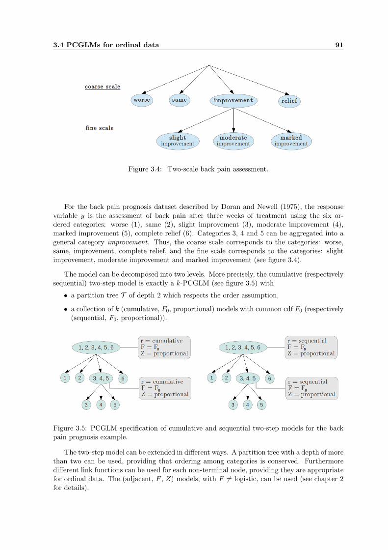
3.4 PCGLMs for ordinal data 91
Figure 3.4: Two-scale back pain assessment.
For the back pain prognosis dataset described by Doran and Newell (1975), the responsevariable y is the assessment of back pain after three weeks of treatment using the six or-dered categories: worse (1), same (2), slight improvement (3), moderate improvement (4),marked improvement (5), complete relief (6). Categories 3, 4 and 5 can be aggregated into ageneral category improvement. Thus, the coarse scale corresponds to the categories: worse,same, improvement, complete relief, and the fine scale corresponds to the categories: slightimprovement, moderate improvement and marked improvement (see figure 3.4).
The model can be decomposed into two levels. More precisely, the cumulative (respectivelysequential) two-step model is exactly a k-PCGLM (see figure 3.5) with
• a partition tree T of depth 2 which respects the order assumption,
• a collection of k (cumulative, F0, proportional) models with common cdf F0 (respectively(sequential, F0, proportional)).
Figure 3.5: PCGLM specification of cumulative and sequential two-step models for the backpain prognosis example.
The two-step model can be extended in different ways. A partition tree with a depth of morethan two can be used, providing that ordering among categories is conserved. Furthermoredifferent link functions can be used for each non-terminal node, providing they are appropriatefor ordinal data. The (adjacent, F , Z) models, with F 6= logistic, can be used (see chapter 2for details).
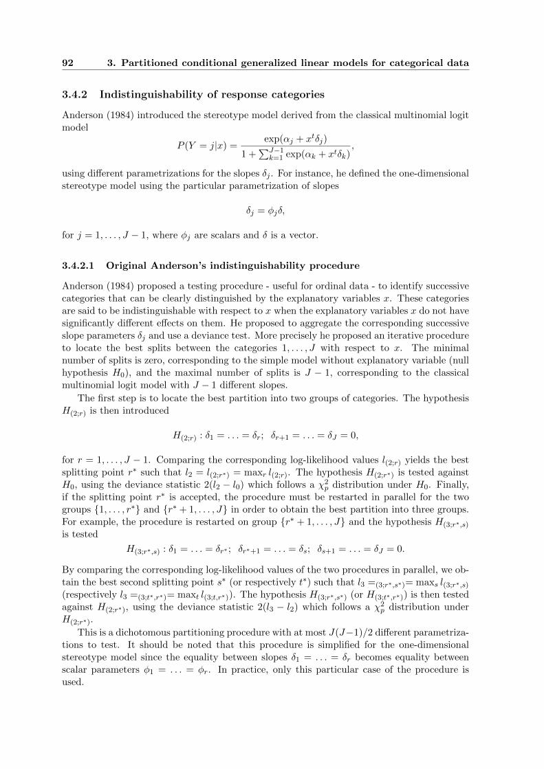
92 3. Partitioned conditional generalized linear models for categorical data
3.4.2 Indistinguishability of response categories
Anderson (1984) introduced the stereotype model derived from the classical multinomial logitmodel
P (Y = j|x) =exp(αj + xtδj)
1 +∑J−1
k=1 exp(αk + xtδk),
using different parametrizations for the slopes δj . For instance, he defined the one-dimensionalstereotype model using the particular parametrization of slopes
δj = φjδ,
for j = 1, . . . , J − 1, where φj are scalars and δ is a vector.
3.4.2.1 Original Anderson’s indistinguishability procedure
Anderson (1984) proposed a testing procedure - useful for ordinal data - to identify successivecategories that can be clearly distinguished by the explanatory variables x. These categoriesare said to be indistinguishable with respect to x when the explanatory variables x do not havesignificantly different effects on them. He proposed to aggregate the corresponding successiveslope parameters δj and use a deviance test. More precisely he proposed an iterative procedureto locate the best splits between the categories 1, . . . , J with respect to x. The minimalnumber of splits is zero, corresponding to the simple model without explanatory variable (nullhypothesis H0), and the maximal number of splits is J − 1, corresponding to the classicalmultinomial logit model with J − 1 different slopes.
The first step is to locate the best partition into two groups of categories. The hypothesisH(2;r) is then introduced
H(2;r) : δ1 = . . . = δr; δr+1 = . . . = δJ = 0,
for r = 1, . . . , J − 1. Comparing the corresponding log-likelihood values l(2;r) yields the bestsplitting point r∗ such that l2 = l(2;r∗) = maxr l(2;r). The hypothesis H(2;r∗) is tested againstH0, using the deviance statistic 2(l2 − l0) which follows a χ2
p distribution under H0. Finally,if the splitting point r∗ is accepted, the procedure must be restarted in parallel for the twogroups 1, . . . , r∗ and r∗ + 1, . . . , J in order to obtain the best partition into three groups.For example, the procedure is restarted on group r∗ + 1, . . . , J and the hypothesis H(3;r∗,s)
is tested
H(3;r∗,s) : δ1 = . . . = δr∗ ; δr∗+1 = . . . = δs; δs+1 = . . . = δJ = 0.
By comparing the corresponding log-likelihood values of the two procedures in parallel, we ob-tain the best second splitting point s∗ (or respectively t∗) such that l3 =(3;r∗,s∗)= maxs l(3;r∗,s)
(respectively l3 =(3;t∗,r∗)= maxt l(3;t,r∗)). The hypothesis H(3;r∗,s∗) (or H(3;t∗,r∗)) is then testedagainst H(2;r∗), using the deviance statistic 2(l3 − l2) which follows a χ2
p distribution underH(2;r∗).
This is a dichotomous partitioning procedure with at most J(J−1)/2 different parametriza-tions to test. It should be noted that this procedure is simplified for the one-dimensionalstereotype model since the equality between slopes δ1 = . . . = δr becomes equality betweenscalar parameters φ1 = . . . = φr. In practice, only this particular case of the procedure isused.

3.4 PCGLMs for ordinal data 93
3.4.2.2 Indistinguishability procedure with (r, F, Z) specification
Here we express the indistinguishability procedure in terms of canonical models by simplychanging the design matrix. In fact, the hypothesis H(2;r) corresponds to the canonical (refer-ence, logistic, Zr) model (see chapter 2) with
Zr =
1 xt
. . ....
. . . xt
. . .
1
,
the design matrix with r repetitions of xt, whereas the null hypothesis H0 corresponds to the(J − 1)-identity design matrix. If the first splitting point r∗ is accepted, the procedure isrestarted to test the hypothesis H(3;r∗,s) which corresponds to the (reference, logistic, Zr∗,s)model with
Zr∗,s =
1 xt
. . ....
. . . xt
. . . xt
. . ....
. . . xt
. . .
1
,
the design matrix with r∗ repetitions of xt for the first block and s − r∗ repetitions of xt forthe second block. The indistinguishability procedure, specified in terms of the (r, F, Z) triplet,can be seen as a design matrix selection procedure.
3.4.2.3 Indistinguishability procedure with PCGLM specification
Here we express the indistinguishability procedure in terms of PCGLM by simply changingthe partition tree. In fact any canonical (reference, logistic, Z) model with a block structureddesign matrix Z is equivalent to a PCGLM of depth 2 with the canonical (reference, logistic,complete) model for the root and minimal response models for other non-terminal nodes. Letus describe this result in detail using the block structured design matrix Zr,s.
Lemma 1. The canonical model (reference, logistic, Zr,s) is equivalent to the PCGLM specifiedin figure 3.6.
Proof. Assume that the distribution of Y |X = x is defined by the canonical (reference, logistic,Zr,s) model. We thus obtain
πjπJ
=
exp(αj + xtδ1), 1 ≤ j ≤ r,exp(αj + xtδ2), r < j ≤ s,exp(αj), s < j ≤ J − 1.
(3.4)
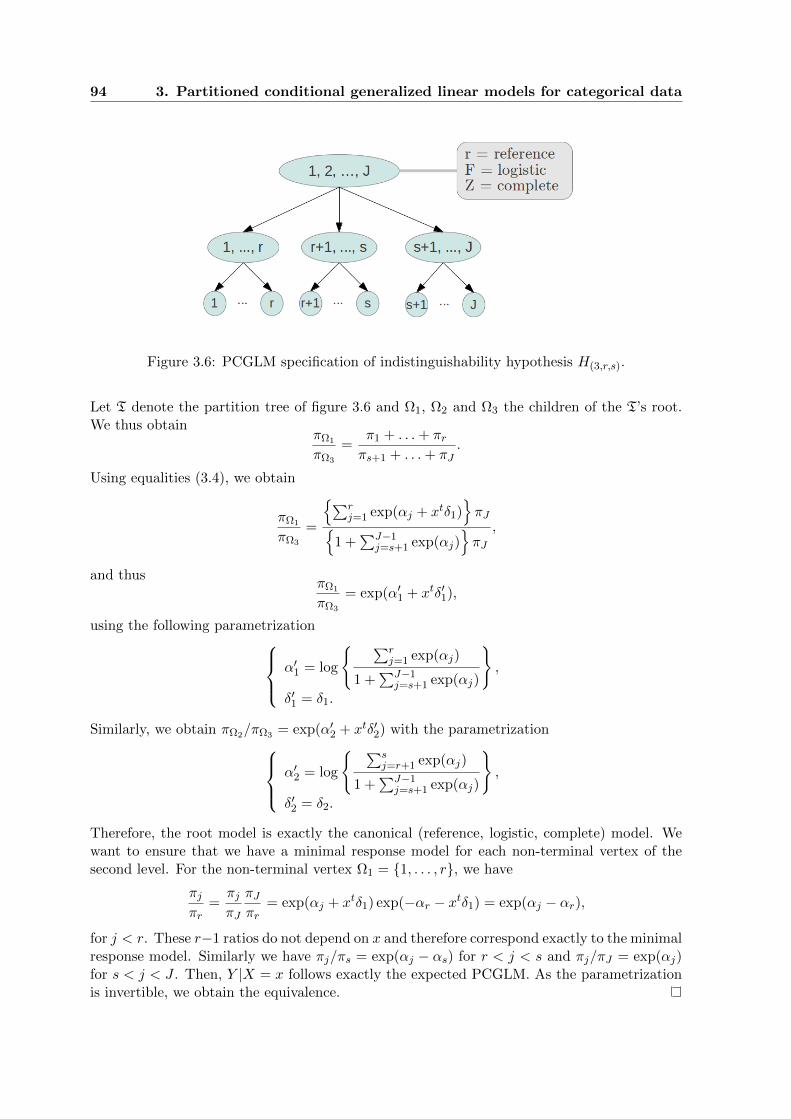
94 3. Partitioned conditional generalized linear models for categorical data
Figure 3.6: PCGLM specification of indistinguishability hypothesis H(3,r,s).
Let T denote the partition tree of figure 3.6 and Ω1, Ω2 and Ω3 the children of the T’s root.We thus obtain
πΩ1
πΩ3
=π1 + . . .+ πrπs+1 + . . .+ πJ
.
Using equalities (3.4), we obtain
πΩ1
πΩ3
=
∑rj=1 exp(αj + xtδ1)
πJ
1 +∑J−1
j=s+1 exp(αj)πJ
,
and thusπΩ1
πΩ3
= exp(α′1 + xtδ′1),
using the following parametrization α′1 = log
∑rj=1 exp(αj)
1 +∑J−1
j=s+1 exp(αj)
,
δ′1 = δ1.
Similarly, we obtain πΩ2/πΩ3 = exp(α′2 + xtδ′2) with the parametrization α′2 = log
∑sj=r+1 exp(αj)
1 +∑J−1
j=s+1 exp(αj)
,
δ′2 = δ2.
Therefore, the root model is exactly the canonical (reference, logistic, complete) model. Wewant to ensure that we have a minimal response model for each non-terminal vertex of thesecond level. For the non-terminal vertex Ω1 = 1, . . . , r, we have
πjπr
=πjπJ
πJπr
= exp(αj + xtδ1) exp(−αr − xtδ1) = exp(αj − αr),
for j < r. These r−1 ratios do not depend on x and therefore correspond exactly to the minimalresponse model. Similarly we have πj/πs = exp(αj − αs) for r < j < s and πj/πJ = exp(αj)for s < j < J . Then, Y |X = x follows exactly the expected PCGLM. As the parametrizationis invertible, we obtain the equivalence.
3.5 PCGLMs for partially-ordered data 95
Using this equivalence, the canonical (reference, logistic, Zr,s) model is easily estimated.In fact, we need to transform the data, aggregating the response categories according to thepartitioning sets Ω1 = 1, . . . , r, Ω2 = r+1, . . . , s and Ω3 = s+1, . . . , J. We then simplyneed to estimate the canonical (reference, logistic, complete) model using this new dataset(and also the three minimal response models of vertices Ω1, Ω2 and Ω3).
3.4.2.4 Extended indistinguishability procedure with PCGLM
The indistinguishability procedure specified with PCGLM can be viewed as a partitioningprocedure. With this form, we see that the procedure uses the ordering assumption to partitionthe categories (only successive categories are aggregated) but the root model does not usethe ordering assumption among the groups of categories. The canonical (reference, logistic,complete) model is appropriate for nominal categories (see chapter 2). Thus, we can definethe same procedure with an ordinal model for the root, such as an adjacent (without logisticcdf), a cumulative, or a sequential model (see chapter 2). Some convergence problems ofthe Fisher’s scoring algorithm may appear for cumulative models because the constraintsηj(x) < ηj+1(x) are more difficult to check with a complete design matrix. Thus, we proposeto use the indistinguishability procedure with the (cumulative, logistic, proportional) model toavoid these difficulties. Our procedure is more comparable to Anderson’s procedure since heused the stereotype logit model which is often more parsimonious than the multinomial logitmodel (between proportional and complete design matrices).
Assume that we apply this procedure and we determine the best root partition for thevector x of explanatory variables. We can say that categories of the same non-terminal vertexare indistinguishable with respect to x. But what about indistinguishability with respect to asubset of x? We therefore propose to select the best subset of x for each non-terminal node.If this subset is non-empty, the procedure is restarted, otherwise the procedure is stopped. Afinal refinement step is then used to select F in each non-terminal vertex to obtain a betterfit. We illustrate this procedure with the back pain prognosis example in section 3.6.1.
3.5 PCGLMs for partially-ordered data
3.5.1 PCGLM specification of the POS-PCM
In categorical data analysis, the case of nominal and ordinal data has already been investigatedin depth while the case of partially-ordered data has been comparatively neglected. Zhang andIp (2012) introduced the partitioned conditional model for partially-ordered set (POS-PCM).The main idea was to recursively partition the J categories in order to obtain either ordinalor nominal models at each step. Zhang and Ip (2012) then used the odds proportional logitmodel for the total order case and the multinomial logit model for the no order case.
Zhang and Ip introduced the partially-ordered set theory into the GLM framework. Apartially-ordered set (poset) (P,) is summarized by a Hasse diagram. The order relationj k is represented by an edge between the two vertices (categories) and vertex k is abovevertex j. A chain in a poset (P,) is a totally ordered subset C of P , whereas an antichain isa set A of pairwise incomparable elements. Zhang and Ip defined an algorithm for categoriespartitioning which gave the following result:
Property 15. (Zhang and Ip, 2012) A finite poset can always be partitioned into antichainsthat are totally weakly ordered.

96 3. Partitioned conditional generalized linear models for categorical data
For any poset (with one component), there exists a partition tree T of depth 2 such thatthe siblings of the first level are totally weakly ordered and the siblings of the second level arenot comparable. The categories are partitioned according to each level of the Hasse diagram(each level is an antichain). Since the antichains are totally (weakly) ordered between them,Zhang and Ip proposed using the odds proportional logit model. Within each antichain, thecategories are not comparable, thus they proposed using the multinomial logit model.
It should be noted that Property 15 holds only if the poset has one component. If thereare two or more components, they must first be partitioned. Since these components arenot comparable, they form an antichain. Thus, a previous level must be added to separateeach component, using the multinomial logit model, and Property 15 must be used for eachcomponent. The depth of the partition tree is exactly 2 if the poset has exactly one component,otherwise it is 3. Finally, for any poset, Zhang and Ip (2012) proposed to associate a particularpartitioned conditional model. This model is a particular PCGLM with
• A partition tree T built from the Hasse diagram.
• A collection C which alternates between the ordinal (cumulative, logistic, proportional)model and the nominal (reference, logistic, complete) model.
Figure 3.7 illustrates this association between a poset (equivalently an Hasse diagram) andthe POS-PCM.
Figure 3.7: Association between an Hasse diagram and a POS-PCM (specified in the PCGLMframework).
3.5.2 Inference of PCGLMs for partially-ordered data
3.5.2.1 Poset structure and partition tree
Zhang and Ip (2012) used poset structure information to define the POS-PCM. But how isthis poset obtained? It is usual to have a nominal or ordinal response variable, but what doesa partially-ordered variable mean? In fact, every partially-ordered variable Y can be expressedin terms of elementary ordinal or nominal variables Yi (with at least one ordinal variable). Forexample, let Y = (Y1, Y2) be a pair of ordinal variables. Let a, b, c be the ordered categoriesof Y1, and 1, 2, 3 be the ordered categories of Y2. The ordering relationship for Y depends onthe relation between Y1 and Y2.

3.5 PCGLMs for partially-ordered data 97
Y1 and Y2 are not comparable In this case the Cartesian product order is used. Let yand y′ be two observed responses. The Cartesian product order C is defined by
y C y′ if(y1 y′1 and y2 y′2
).
In this case we can use the Property 15 to obtain the partition tree from the Hasse diagramin figure 3.8.
Figure 3.8: Hasse diagram of Cartesian product order and corresponding partition tree.
Y1 and Y2 are ordered In this case the lexicographic order has to be used. Assume thatY1 Y2 and let y and y′ be two observed responses. The lexicographic order L is defined by
y L y′ if(y1 y′1
)or(y1 = y′1 and y2 y′2
).
In this case the order among the response categories is total. But a 2-partition tree seems tobe appropriated: with a first level for Y1 and a second level for Y2|Y1 (see figure 3.9). Theorder among latent variables (shown in red) seems to have priority over the order among cat-egories (shown in blue). A common slope δ can be considered (see section 3.2.3 for parameterestimation) because the same response variable Y2 is involved in all the non-terminal verticesof the second level.
Figure 3.9: Hasse diagram of lexicographic order and corresponding partition tree.

98 3. Partitioned conditional generalized linear models for categorical data
3.5.2.2 Collection of models C
Given a non-terminal vertex v of T, we choose an ordinal model if the children of v are totallyordered. Otherwise we choose a nominal model. In this way Zhang and Ip (2012) used the oddsproportional logit model in the ordinal case and the multinomial logit model in the nominalcase. More generally, we propose to use the families of cumulative, sequential and adjacent(without logistic distribution) models for ordinal data and the family of reference models fornominal data (see chapter 2).
3.6 Applications
3.6.1 Totally ordered data: back pain prognosis example
Doran and Newell (1975) described a back pain study involving 101 patients. The responsevariable y was the assessment of back pain after three weeks of treatment using the six orderedcategories: worse (1), same (2), slight improvement (3), moderate improvement (4), markedimprovement (5), complete relief (6). The three selected explanatory variables observed at thebeginning of the treatment period were x1 = length of previous attack (1=short, 2=long), x2 =pain change (1=getting better, 2=same, 3=worse) and x3 = lordosis (1=absent/decreasing,2=present/increasing).
Here, the response categories are defined by the experimentalist and this ordinal scale maythus not be the most efficient to describe the back pain prognosis of a patient. Firstly, we willuse the hierarchy among the categories shown in figure 3.4 and select the best regression modelfor it. Secondly, we will select the hierarchy and at the same time the explanatory variables,using our extended indistinguishability procedure. We will thus compare the two results andthe result obtained by Anderson (1984).
The case of known partition tree T
Here, the partition tree is a priori defined with worse, same, improvement, complete reliefat the first level, with improvement being partitioned into slight improvement, moderateimprovement, marked improvement at the second level; see figure 3.4. We must select thebest GLM for the root of T and the non-terminal vertex slight improvement, moderate im-provement, marked improvement. For these two vertices we have an ordinal scale, thus themost appropriate ratios are adjacent and cumulative. We chose the adjacent ratio in orderto avoid algorithm difficulties with the complete design matrix, and the symmetric normalcdf, appropriate for ordinal data (see chapter 2 for details). Since there were at most K = 3explanatory variables, we compared all 23 combinations. Complete and proportional designmatrices were tested for each combination. The variable x1 was the only one selected for thetwo vertices with the complete design matrix. Since this explanatory variable was categorical,the model was exactly the saturated model. Therefore all the link functions were equivalent.Finally, the maximised log-likelihood was l = −161.14 for 10 parameters. This partition treedoes not seem to be appropriate for the data as only x1 was selected for it, whereas x1, x2,x3 were selected for the canonical 1-partition tree. More precisely, the simple (cumulative, lo-gistic, proportional) model had a log-likelihood of −159.045 for 8 parameters, using the threeexplanatory variables.
3.6 Applications 99
The case of unknown partition tree T
We will use this dataset to illustrate the extended indinguishability procedure which corre-sponds to a partition tree and variable selection procedure. Since T must respect categoryordering, the space of possible partition trees is reduced. During the procedure, only the or-dinal (cumulative, logistic, proportional) model and the minimal response model (i.e. withoutexplanatory variable) will be used in the collection C.
First level Note that every PCGLM with only a root proportional model (and minimalresponse models for other non-terminal nodes) have exactly the same number of parameters:J − 1 + p = 8. Thus, we simply use the log-likelihood to compare these models. We begin theprocedure with the the simple model M0 = (cumulative, logistic, proportional) which can beseen to be a 1-PCGLM. The corresponding log-likelihood is l0 = −159.046.
Here we are looking for the best splitting point r ∈ 1, 2, 3, 4, 5 for explanatory variablesx1, x2 and x3. Note that model M0 corresponds exactly to the splitting point r = J − 1 = 5since all the J − 1 slopes are common in this case. The best model is obtained for r∗ = 4 withlog-likelihood lr∗ = −158.132. Since lr∗ > l0, the splitting point r∗ is selected. We now look forthe best splitting point s ∈ 1, 2, 3 ∪ 5 that gives three nodes. The best model is obtainedfor s∗ = 1 with log-likelihood ls∗,r∗ = −155.756. Since ls∗,r∗ > lr∗ , the second splitting points∗ is also selected. As every partitions in four groups are rejected, the best root partition is1 ∪ 2, 3, 4 ∪ 5, 6 for explanatory variables x1, x2,x3.
Second level We now focus on the non-terminal vertices v1 = 2, 3, 4 and v2 = 5, 6.We first select the subset of influential explanatory variables for these two nodes, using againthe simple (cumulative, logistic, proportional) model with the Bayesian Information Criteria(BIC). As previously seen, the different models of collection C can be estimated separatelybecause the parameter βv is different for each non-terminal vertex v. The explanatory variablex2 is selected for vertex v1 and no variable is selected for vertex v2. For vertex v2, the minimalresponse model has a log-likelihood lv2 = −28.841. Thus, we simply focus on vertex v1 andobtain a log-likelihood lv10 = −54.561 with the simple (cumulative, logistic, proportional)model, using only x2.
We now look for the best splitting point t ∈ 2, 3, 4 of vertex v1 for the explanatoryvariable x2. The best model is obtained for t∗ = 3 with a log-likelihood lv1t∗ = −54.31. Sincelv1t∗ > lv10 , the splitting point t∗ is selected. This is the last possible partition for the secondlevel of the partition tree.
Last level and refinement step There is only the vertex v3 = 2, 3 at the third level withonly the explanatory variable x2. Since we have to reduce the set of explanatory variables,the minimal response model is estimated for this vertex with log-likelihood lv3 = −21.93. Theselection procedure of the partition tree and the explanatory variables is then stopped. Thecorresponding log-likelihood is l = −153.418 for 9 parameters, with the logistic cdf for eachnode. We then execute a refinement step by selecting the best cdf F for each vertex anddetermine the modelM∗ (see figure 3.10) with log-likelihood l∗ = −152.727 for 9 parameters.
Looking at the results obtained in the first part, it can be seen that the categories do notappear to be appropriate for describing back pain. In fact, in the second part, our results aresimilar to those of Anderson for the first step of the model: i.e. the partition worse, same,little imp., moderate imp., slight imp., complete relief for the three explanatory variables.He obtained a log-likelihood of −154.39 for 9 parameters. Our methodology allows us to go a
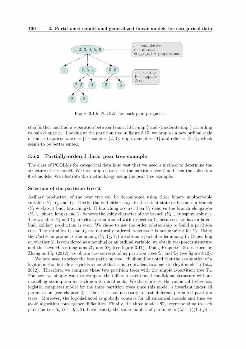
100 3. Partitioned conditional generalized linear models for categorical data
Figure 3.10: PCGLM for back pain prognosis.
step further and find a separation between same, little imp. and moderate imp. accordingto pain change x2. Looking at the partition tree in figure 3.10, we propose a new ordinal scaleof four categories: worse = 1, same = 2, 3, improvement = 4 and relief = 5, 6, whichseems to be better suited.
3.6.2 Partially-ordered data: pear tree example
The class of PCGLMs for categorical data is so vast that we need a method to determine thestructure of the model. We first propose to select the partition tree T and then the collectionC of models. We illustrate this methodology using the pear tree example.
Selection of the partition tree T
Axillary production of the pear tree can be decomposed using three binary unobservablevariables Y1, Y2 and Y3. Firstly, the bud either stays in the latent state or becomes a branch(Y1 ∈ latent bud, branching). If branching occurs, then Y2 denotes the branch elongation(Y2 ∈ short, long) and Y3 denotes the spiny character of the branch (Y3 ∈ unspiny, spiny).The variables Y2 and Y3 are clearly conditioned with respect to Y1 because if we have a latentbud, axillary production is over. We chose to use the order relationship to build a partitiontree. The variables Y1 and Y2 are naturally ordered, whereas it is not manifest for Y3. Usingthe Cartesian product order among (Y1, Y2, Y3) we obtain a partial order among Y . Dependingon whether Y3 is considered as a nominal or an ordinal variable, we obtain two posets structureand thus two Hasse diagrams D1 and D2 (see figure 3.11). Using Property 15 described byZhang and Ip (2012), we obtain two corresponding partition trees T1 and T2 (see figure 3.12).
We now need to select the best partition tree. “It should be noted that the assumption of alogit model on both levels yields a model that is not equivalent to a one-step logit model” (Tutz,2012). Therefore, we compare these two partition trees with the simple 1-partition tree T0.For now, we simply want to compare the different partitioned conditional structure withoutmodelling assumption for each non-terminal node. We therefore use the canonical (reference,logistic, complete) model for the three partition trees since this model is invariant under allpermutation (see chapter 2). Thus it is not necessary to test different permuted partitiontrees. Moreover, the log-likelihood is globally concave for all canonical models and thus weavoid algorithm convergence difficulties. Finally, the three models Mi, corresponding to eachpartition tree Ti (i = 0, 1, 2), have exactly the same number of parameters ((J − 1)(1 + p) =
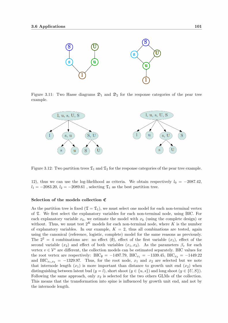
3.6 Applications 101
Figure 3.11: Two Hasse diagrams D1 and D2 for the response categories of the pear treeexample.
Figure 3.12: Two partition trees T1 and T2 for the response categories of the pear tree example.
12), thus we can use the log-likelihood as criteria. We obtain respectively l0 = −2087.42,l1 = −2083.20, l2 = −2089.61 , selecting T1 as the best partition tree.
Selection of the models collection C
As the partition tree is fixed (T = T1), we must select one model for each non-terminal vertexof T. We first select the explanatory variables for each non-terminal node, using BIC. Foreach explanatory variable xk, we estimate the model with xk (using the complete design) orwithout. Thus, we must test 2K models for each non-terminal node, where K is the numberof explanatory variables. In our example, K = 2, thus all combinations are tested, againusing the canonical (reference, logistic, complete) model for the same reasons as previously.The 22 = 4 combinations are: no effect (∅), effect of the first variable (x1), effect of thesecond variable (x2) and effect of both variables (x1, x2). As the parameters βv for eachvertex v ∈ V∗ are different, the collection models can be estimated separately. BIC values forthe root vertex are respectively: BIC∅ = −1497.79, BICx1 = −1339.45, BICx2 = −1449.22and BICx1,x2 = −1329.97. Thus, for the root node, x1 and x2 are selected but we notethat internode length (x1) is more important than distance to growth unit end (x2) whendistinguishing between latent bud (y = l), short shoot (y ∈ u, s) and long shoot (y ∈ U, S).Following the same approach, only x2 is selected for the two others GLMs of the collection.This means that the transformation into spine is influenced by growth unit end, and not bythe internode length.
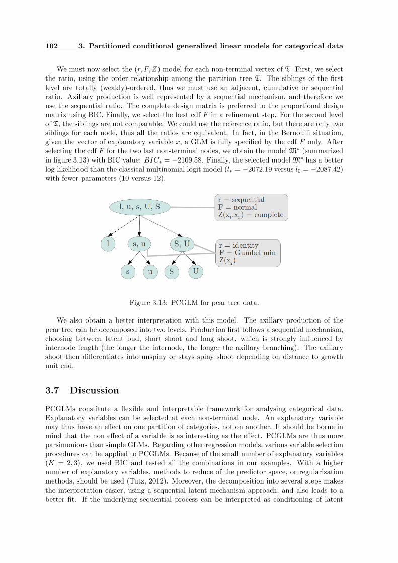
102 3. Partitioned conditional generalized linear models for categorical data
We must now select the (r, F, Z) model for each non-terminal vertex of T. First, we selectthe ratio, using the order relationship among the partition tree T. The siblings of the firstlevel are totally (weakly)-ordered, thus we must use an adjacent, cumulative or sequentialratio. Axillary production is well represented by a sequential mechanism, and therefore weuse the sequential ratio. The complete design matrix is preferred to the proportional designmatrix using BIC. Finally, we select the best cdf F in a refinement step. For the second levelof T, the siblings are not comparable. We could use the reference ratio, but there are only twosiblings for each node, thus all the ratios are equivalent. In fact, in the Bernoulli situation,given the vector of explanatory variable x, a GLM is fully specified by the cdf F only. Afterselecting the cdf F for the two last non-terminal nodes, we obtain the model M∗ (summarizedin figure 3.13) with BIC value: BIC∗ = −2109.58. Finally, the selected model M∗ has a betterlog-likelihood than the classical multinomial logit model (l∗ = −2072.19 versus l0 = −2087.42)with fewer parameters (10 versus 12).
Figure 3.13: PCGLM for pear tree data.
We also obtain a better interpretation with this model. The axillary production of thepear tree can be decomposed into two levels. Production first follows a sequential mechanism,choosing between latent bud, short shoot and long shoot, which is strongly influenced byinternode length (the longer the internode, the longer the axillary branching). The axillaryshoot then differentiates into unspiny or stays spiny shoot depending on distance to growthunit end.
3.7 Discussion
PCGLMs constitute a flexible and interpretable framework for analysing categorical data.Explanatory variables can be selected at each non-terminal node. An explanatory variablemay thus have an effect on one partition of categories, not on another. It should be borne inmind that the non effect of a variable is as interesting as the effect. PCGLMs are thus moreparsimonious than simple GLMs. Regarding other regression models, various variable selectionprocedures can be applied to PCGLMs. Because of the small number of explanatory variables(K = 2, 3), we used BIC and tested all the combinations in our examples. With a highernumber of explanatory variables, methods to reduce of the predictor space, or regularizationmethods, should be used (Tutz, 2012). Moreover, the decomposition into several steps makesthe interpretation easier, using a sequential latent mechanism approach, and also leads to abetter fit. If the underlying sequential process can be interpreted as conditioning of latent
3.7 Discussion 103
variables (Y2|Y1 ∈ v and Y2|Y1 ∈ v′), a common effect on two vertices (βv = βv′) can be
considered.Except in this last case, PCGLMs can be easily estimated. After rearranging the data by
partitioning and conditioning, classical algorithms can be applied for each data subset. Forthe simplest and most common case βv 6= βv
′, the different algorithms may be parallelized
and running time is thus reduced. Moreover, a canonical GLM with a block structured designmatrix can be written as a PCGLM with simple design matrices (see lemma 1) that is easierto estimate.
An important issue with PCGLMs is selecting the partition tree. The tree may be deter-mined a priori, as in classical approaches. The two-step model, for instance, relies on an apriori known hierarchy among ordered categories. The nested logit model aggregates cate-gories that are similar (i.e. influenced by the same variables). Finally, a POS-PCM associatesa partition tree to a Hasse diagram (poset). But defining this poset from the correspondinglatent process is not an easy task. In most applications the partition tree is not a prioriknown and should thus be selected. The proposed approach for selecting the partition treeand the variables could be used in the supervised classification context with ordered classes.The indistinguishability procedure selects the best splitting between categories, starting fromthe entire set 1, . . . , J. Alternatively, we may aggregate adjacent categories, starting fromsingletons j.
Finally, caution should be exercised to penalize log-likelihood. Let us consider the contextof BIC penalization. The total number of observations n should a priori be used. But if anexplanatory variable influences a non terminal vertex v associated with a small proportion ofthe observations (nv n), should we incorporate a term related to nv in the penalty?

Chapter 4
Integrative models for jointlyanalyzing shoot growth and
branching patterns
Abstract
Background and Aims: It has long been known that shoot growth has an effect on its branchingpatterns, but the characterization of the corresponding patterning mechanism is still an openissue.Methods: Dedicated statistical models, called semi-Markov switching partitioned conditionalgeneralized linear models, were applied to apple and pear tree data sets. In the semi-Markovswitching partitioned conditional generalized linear models estimated from these data sets, theunderlying semi-Markov chain represents both the succession and lengths of branching zones,while the partitioned conditional generalized linear models represent the influence of growthexplanatory variables on axillary productions within each branching zone.Key results: On the basis of these integrative statistical models, we show that smoothed anddelayed growth explanatory variables influence specific branching events.Conclusions: The partitioned conditional generalized linear model selected for each branchingzone can be used to identify which developmental event (e.g. shoot initiation, shoot elongationor apex transformation into spine) is affected by a given explanatory variable. The proposedintegrative statistical modelling approach could incorporate other explanatory variables suchas local curvature of the parent shoot or maximum growth rate of the internode or leaf.
Keywords: branching pattern, categorical data, generalized linear model, growth pattern,semi-Markov switching regression model.
Contents
4.1 Introduction . . . . . . . . . . . . . . . . . . . . . . . . . . . . . . . . . . 106
4.2 Materials and methods . . . . . . . . . . . . . . . . . . . . . . . . . . . . 106
4.2.1 Tree data sets . . . . . . . . . . . . . . . . . . . . . . . . . . . . . . . . . . 106
4.2.2 Models . . . . . . . . . . . . . . . . . . . . . . . . . . . . . . . . . . . . . 107
4.3 Results . . . . . . . . . . . . . . . . . . . . . . . . . . . . . . . . . . . . . . 108
4.3.1 Apple tree . . . . . . . . . . . . . . . . . . . . . . . . . . . . . . . . . . . . 108
4.3.2 Pear tree . . . . . . . . . . . . . . . . . . . . . . . . . . . . . . . . . . . . 111
4.4 Discussion . . . . . . . . . . . . . . . . . . . . . . . . . . . . . . . . . . . . 116
106 4. Integrative models for analyzing shoot growth and branching patterns
4.1 Introduction
Soot branching patterns often take the form of a succession of well-differentiated homogeneousbranching zones where composition properties, in terms of axillary productions, do not changesubstantially within each zone, but change markedly between zones. These branching patternshave been analysed using segmentation models and in particular hidden semi-Markov chains(Guedon et al., 2001). Branching patterns are modulated by factors that have an overall effecton the pattern, and by factors that vary along the shoot and have differentiated effects onsuccessive axillary productions. We previously investigated the influence of the architecturalposition of a shoot, which can be viewed as a factor that have an overall effect, on apple treebranching patterns (Renton et al., 2006).
Here, we focus on factors that vary along the shoot and modulate its branching pattern.For example, it has been shown that shoot growth modulates branching pattern, in particularimmediate (or sylleptic) branching; see Lauri and Terouanne (1998) for an illustration in theapple tree case. Other potential factors include local curvature of the shoot (Han et al., 2007).To this end, we introduced a new family of integrative statistical models for analysing jointlythe succession and length of branching zones and the modulation of the axillary productionswithin each zone by factors that vary along the shoot. These models generalize hidden semi-Markov chains for categorical data (Guedon et al., 2001) by incorporating explanatory vari-ables and are called semi-Markov switching partitioned conditional generalized linear models(SMS-PCGLMs). It should be noted that another family of semi-Markov switching regressionmodels has been previously introduced for analysing forest tree growth components. Moreprecisely, semi-Markov switching linear mixed models have been used to identify and charac-terize ontogenetic, environmental and individual growth components on the basis of tree mainstems described by annual shoot and climatic data (Chaubert-Pereira et al., 2009).
4.2 Materials and methods
4.2.1 Tree data sets
The proposed approach is illustrated by the analysis of immediate branching patterns in appleand pear trees.
4.2.1.1 Apple tree (Malus domestica Borkh)
Twenty two one-year-old apple trees, “Fuji” cultivar, grafted on M9 (Pajam 1) rootstockand planted at the DiaScope experimental at INRA Montpellier were analysed in this study.Distances between trees corresponded to 3 m between rows and 0.7 m between trees in thesame row. Agricultural practices - including irrigation with micro-sprinklers, fertilization andspraying against pests and diseases - were done according to standard practices in the area.
The one-year-old main axis developed from the graft was described by node. The presenceof an immediate axillary shoot - i.e. developed without delay with respect to the parent nodeestablishment date - was noted at each successive node,. Immediate shoots were classifiedinto two categories, short and long, according to length (≤ 5cm or > 5cm, respectively).Successive internode lengths along the main axis were measured with a tape ruler that wasprecise to within 0.5 cm. This dataset was thus constituted of 22 bivariate sequences ofcumulative length 1494 (length between 63 and 73 nodes) associating a categorical variable(type of axillary production selected from among latent bud, short or long immediate shoot)with an interval-scaled variable (internode length).
4.2 Materials and methods 107
4.2.1.2 Pear tree (Pyrus spinosa)
Harvested seeds of Pyrus spinosa were sown and planted in January 2001 in a nursery locatednear Aix-en-Provence, southeastern France. Seedlings grew in 600cm3 WM containers groupedin plastic crates by 25. In winter 2001, the first annual shoot on the main axis of 50 one-year-old individuals was described by node. In this nursery context, individuals were able to growtwice a year, and the annual shoots were made up of one or two growth units (GU) - i.e.portion of the axis built up during an uninterrupted period of growth - referred to as GU1or GU2 in the following. Seven monocyclic annual shoots (only GU1) and 43 bicyclic annualshoots (GU1 and GU2) were observed.
The presence at each successive node of an immediate axillary shoot was noted. Immediateshoots were classified in four categories according to length (≤ 1cm or > 1cm, with internodesnot distinguishable for short shoots), and to transformation or not of the apex into spine (i.e.definite growth or not). This dataset was thus made up of 50 bivariate sequences of cumulativelength 3285 associating a categorical variable (type of axillary production selected from amonglatent bud, unspiny short, unspiny long, spiny short and spiny long immediate shoot), withan interval-scaled variable (internode length).
4.2.2 Models
A semi-Markov switching partitioned conditional generalized linear model, which is a two-scale segmentation model, was built on the basis of each data set. In this framework, thesuccession and length of branching zones (coarse scale) are represented by a non-observablesemi-Markov chain while the types of axillary productions within each branching zone (finescale) modulated by explanatory variables that vary along the parent shoot are represented bypartitioned conditional generalized linear models attached to each state of the semi-Markovchain. Hence, each state of the semi-Markov chain represents a branching zone. In ourapplication context, the explanatory variables reflect the growth of the parent shoot, but thestatistical framework is general.
The overall model thus combines an A-state semi-Markov chain with A partitioned con-ditional generalized linear models and is referred to as a semi-Markov switching partitionedconditional generalized linear model (SMS-PCGLM). A SMS-PCGLM combines three cate-gories of variables: (i) “state” variable representing non-directly observable branching zones,(ii) plant response categorical variable (types of axillary production), (iii) explanatory variablesthat vary with node rank (e.g. internode length). This family of statistical models broadensthe family of Markov switching models; see Fruhwirth-Schnatter (2006) for an overview ofMarkov switching models.
An A-state semi-Markov chain is defined by three subsets of parameters:
• initial probabilities (ϕa; a = 0, . . . , A− 1) to model which is the first branching zone inthe parent shoot,
• transition probabilities (pa,b; a, b = 0, . . . , A − 1) to model the succession of branchingzones along a parent shoot,
• occupancy distributions attached to non-absorbing states (a state is said to be absorbingif, after entering this state, it is impossible to leave it) to model lengths of branchingzones in number of nodes. We used binomial distributions B(d, n, p), Poisson distribu-tions P(d, λ) and negative binomial distributions NB(d, r, p) as possible parametric state
108 4. Integrative models for analyzing shoot growth and branching patterns
occupancy distributions, with an additional shift parameter d ≥ 1; see Appendix C forformal definitions of these distributions.
In the context of regression models for categorical data analysis, the focus was mainlyon models for nominal response variables (unordered categories) or ordinal response variables(totally ordered categories). Here we adopt a more general framework where the categoriescan be represented as a tree of nested partitions of categories (e.g. latent but versus immediateshoots at the first level, immediate shoots partitioned into short and long at the second levelfor the apple tree example); see Peyhardi et al. (2013b). This framework means we can tacklethe case of partially-ordered response variables and also differentiate the role of explanatoryvariables at different levels of the partition tree (e.g. an explanatory variable influencing theoccurrence of immediate shoots but not their subsequent growth as short or long shoots).
In partitioned conditional generalized linear models, the partition tree of categories andthe explanatory variables relevant for each non-terminal vertex of the partition tree need to beselected. We thus adopted a two-stage approach for inference where in a first stage, a simplehidden semi-Markov chain (i.e. without explanatory variables) was estimated for a given dataset. This estimated hidden semi-Markov chain was used to segment the observed sequencesinto homogeneous branching zones and for each branching zone (except unbranched zoneswhere only latent buds were observed), a PCGLM was selected by identifying the partitiontree and the explanatory variables. In a second stage a SMS-PCGLM was estimated on thebasis of the observed sequences.
4.3 Results
4.3.1 Apple tree
Superimposition of the proportions of immediate shoots (short and long shoots are not dis-tinguished) and pointwise average internode lengths showed that an unbranched zone corre-sponding to short internodes spreading over the first few nodes was followed by a zone whereinternode length increased abruptly. Shoot occurrence also increased abruptly but with a shiftof a few nodes with respect to the increase in internode length (Figure 4.1). Internode lengththen decreased gradually along the parent shoot while the decrease in shoot occurrence wasmore irregular.
We first estimated a 3-state HSMC made up of two transient states (corresponding to anunbranched and a branching zone) followed by a final absorbing end state modelling growthcessation (Renton et al., 2006) on the basis of the observed bivariate sequences, including theinternode length variable. It should be noted that the segmented branching zones obtainedusing only the types of axillary production variable were very similar (98.5% match betweenthe segmentations obtained using the estimated univariate and bivariate HSMCs). We thenextracted the sub-sequences corresponding to the branching zone (state 1). The posteriorprobabilities of the optimal segmentations (i.e. weight of the optimal segmentation among allthe possible segmentations of a given observed sequence) were very high (always above 0.995for the 22 individuals).
As a second step, we selected the explanatory variable using canonical GLMs (multinomiallogit model for nominal data) and then identified the partition tree of categories using theselected explanatory variable on the basis of the data extracted from the branching zone. Wetested two types of transformation of the measured internode length variable to build potentialexplanatory variables:

4.3 Results 109
Figure 4.1: Proportions of immediate shoots (short and long shoots are not distinguished) andpointwise average lengths of internodes as a function of node rank represented on a commony scale whose maximum corresponds to the maximum proportion of immediate shoots and themaximum average length of internodes.
• shift of the variable, in particular backward shifts, since the internode elongation lastsabout 12 days in apple tree and temporally overlaps the initiation of immediate shootsa few nodes below the apex.
• smoothing of the variable to remove fluctuations and extract the local internode lengthtrend. This smoothing can be interpreted as an averaging over internodes that elongateat a given time t.
To this end, canonical GLMs were estimated for each possible explanatory variable. Thebest GLM according to the Bayesian information criterion (BIC) was obtained with no shiftand smoothing of the internode length was obtained using a symmetric smoothing filter cor-responding to the probability mass function of the binomial distribution of parameters 32 and0.5 (95% of the mass concentrated on the 11 central values). This smoothing width appearsto be consistent with the order of magnitude of the number of internodes that elongate at agiven time t. Having selected the explanatory variable, we then identified the partition treeof categories. We obtained a first partition into latent bud and immediate shoots, then asubsequent partition of immediate shoots into short and long shoot; see Figure 4.2.
Finally, a 3-state SMS-PCGLM was estimated using the partition tree and explanatoryvariable previously selected for the PCGLM associated with state 1 (branching zone); seeFigure 4.2. The deterministic succession of states resulted from the iterative estimation proce-dure. The unbranched zone corresponding to short internodes at the base of the shoot (state0) corresponds to the preformed part of the shoot. The fact that the highest probability ofbranching and the longest internodes, were found near the shoot base (around rank 10) likelyresulted from the propagation mode of the observed young plants derived from bud grafting on

110 4. Integrative models for analyzing shoot growth and branching patterns
Figure 4.2: Semi-Markov chain: each state is represented by a vertex which is numbered.Vertices representing transient states are edged by a single line while the vertex representingthe absorbing end state is edged by a double line. The possible transitions between statesare represented by arcs (the attached probabilities are always 1). The arc entering in state 0indicates that it is the only possible initial state. The occupancy distributions of the transientstates are shown above the corresponding vertices. Observation models: for state 0 (unbranchedzone), the observation model is degenerate since the only possible observation is latent bud. Forstate 1 (branched zone), the estimated branching probability p decreases with internode lengthalong the parent shoot. Locally smoothed internode length markedly influences immediate shootinitiation but only slightly influences the subsequent growth of these immediate shoots (and theinfluence of explanatory variable is only shown for the partition latent bud/immediate shoot).
one-year-old rootstock. The locally smoothed internode length markedly influences immediateshoot initiation (first level of the partition tree corresponding to latent bud versus immediateshoot) but only slightly influences the subsequent growth of these immediate shoots (secondlevel of the partition tree corresponding to short versus long shoot); see Figure 4.3.
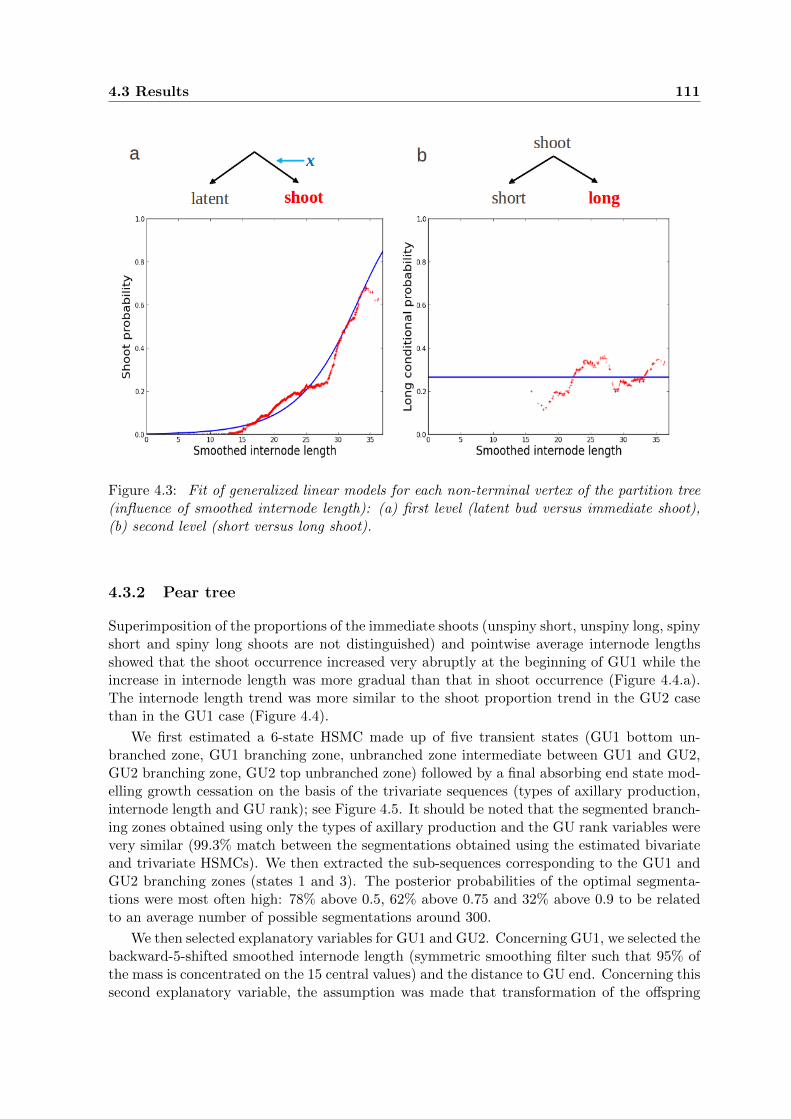
4.3 Results 111
Figure 4.3: Fit of generalized linear models for each non-terminal vertex of the partition tree(influence of smoothed internode length): (a) first level (latent bud versus immediate shoot),(b) second level (short versus long shoot).
4.3.2 Pear tree
Superimposition of the proportions of the immediate shoots (unspiny short, unspiny long, spinyshort and spiny long shoots are not distinguished) and pointwise average internode lengthsshowed that the shoot occurrence increased very abruptly at the beginning of GU1 while theincrease in internode length was more gradual than that in shoot occurrence (Figure 4.4.a).The internode length trend was more similar to the shoot proportion trend in the GU2 casethan in the GU1 case (Figure 4.4).
We first estimated a 6-state HSMC made up of five transient states (GU1 bottom un-branched zone, GU1 branching zone, unbranched zone intermediate between GU1 and GU2,GU2 branching zone, GU2 top unbranched zone) followed by a final absorbing end state mod-elling growth cessation on the basis of the trivariate sequences (types of axillary production,internode length and GU rank); see Figure 4.5. It should be noted that the segmented branch-ing zones obtained using only the types of axillary production and the GU rank variables werevery similar (99.3% match between the segmentations obtained using the estimated bivariateand trivariate HSMCs). We then extracted the sub-sequences corresponding to the GU1 andGU2 branching zones (states 1 and 3). The posterior probabilities of the optimal segmenta-tions were most often high: 78% above 0.5, 62% above 0.75 and 32% above 0.9 to be relatedto an average number of possible segmentations around 300.
We then selected explanatory variables for GU1 and GU2. Concerning GU1, we selected thebackward-5-shifted smoothed internode length (symmetric smoothing filter such that 95% ofthe mass is concentrated on the 15 central values) and the distance to GU end. Concerning thissecond explanatory variable, the assumption was made that transformation of the offspring

112 4. Integrative models for analyzing shoot growth and branching patterns
Figure 4.4: Proportions of immediate shoots (unspiny short, unspiny long, spiny short andspiny long shoots are not distinguished) and pointwise average lengths of the internodes as afunction of node rank represented on a common y scale whose maximum corresponds to themaximum proportion of immediate shoots and the maximum average length of internodes. (a)GU1, (b) GU2.
shoot apex into spine is related to the growth end of the parent shoot. Concerning treepartition, we investigated in particular the partition corresponding to successive developmental
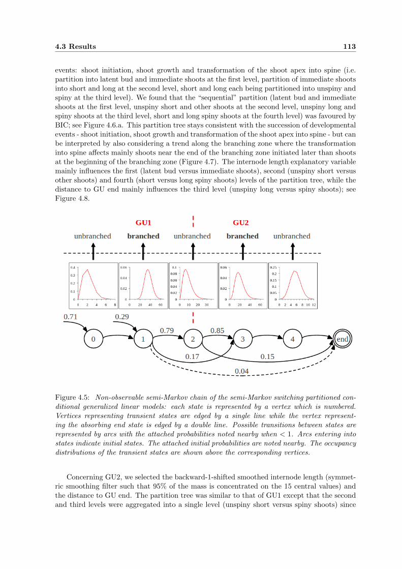
4.3 Results 113
events: shoot initiation, shoot growth and transformation of the shoot apex into spine (i.e.partition into latent bud and immediate shoots at the first level, partition of immediate shootsinto short and long at the second level, short and long each being partitioned into unspiny andspiny at the third level). We found that the “sequential” partition (latent bud and immediateshoots at the first level, unspiny short and other shoots at the second level, unspiny long andspiny shoots at the third level, short and long spiny shoots at the fourth level) was favoured byBIC; see Figure 4.6.a. This partition tree stays consistent with the succession of developmentalevents - shoot initiation, shoot growth and transformation of the shoot apex into spine - but canbe interpreted by also considering a trend along the branching zone where the transformationinto spine affects mainly shoots near the end of the branching zone initiated later than shootsat the beginning of the branching zone (Figure 4.7). The internode length explanatory variablemainly influences the first (latent bud versus immediate shoots), second (unspiny short versusother shoots) and fourth (short versus long spiny shoots) levels of the partition tree, while thedistance to GU end mainly influences the third level (unspiny long versus spiny shoots); seeFigure 4.8.
Figure 4.5: Non-observable semi-Markov chain of the semi-Markov switching partitioned con-ditional generalized linear models: each state is represented by a vertex which is numbered.Vertices representing transient states are edged by a single line while the vertex represent-ing the absorbing end state is edged by a double line. Possible transitions between states arerepresented by arcs with the attached probabilities noted nearby when < 1. Arcs entering intostates indicate initial states. The attached initial probabilities are noted nearby. The occupancydistributions of the transient states are shown above the corresponding vertices.
Concerning GU2, we selected the backward-1-shifted smoothed internode length (symmet-ric smoothing filter such that 95% of the mass is concentrated on the 15 central values) andthe distance to GU end. The partition tree was similar to that of GU1 except that the secondand third levels were aggregated into a single level (unspiny short versus spiny shoots) since

114 4. Integrative models for analyzing shoot growth and branching patterns
unspiny long shoots were very rare in GU2 (17 out of 794 immediate shoots) and were thusnot considered in the identification of the partition tree. The internode length explanatoryvariable influences all three levels (latent bud versus immediate shoots, unspiny short versusspiny shoots, short versus long spiny shoots) of the partition tree, while the distance to GUend mainly influences the last two levels; see Figure 4.6.b.
Figure 4.6: Partitioned conditional generalized linear models for (a) GU1 branching zone and(b) GU2 branching zone.
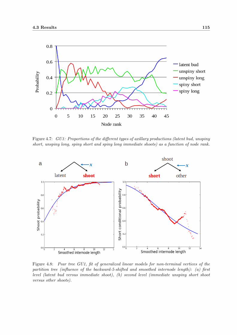
4.3 Results 115
Figure 4.7: GU1: Proportions of the different types of axillary productions (latent bud, unspinyshort, unspiny long, spiny short and spiny long immediate shoots) as a function of node rank.
Figure 4.8: Pear tree GU1, fit of generalized linear models for non-terminal vertices of thepartition tree (influence of the backward-5-shifted and smoothed internode length): (a) firstlevel (latent bud versus immediate shoot), (b) second level (immediate unspiny short shootversus other shoots).
116 4. Integrative models for analyzing shoot growth and branching patterns
4.4 Discussion
The examples given above illustrate how the definition of appropriate explanatory variables isa crucial step in retrospective measurements. We are currently investigating the extraction ofexplanatory variables based on growth data follow up (e.g. leaf expansion). In this context, theextraction of explanatory variables requires two steps, (i) extraction of growth parameters usingfor instance nonlinear regression models (e.g. the maximum absolute growth rate deduced fromthe fit of a sigmoidal function), (ii) the shifting and smoothing of growth parameters deducedfrom nonlinear regression models. This transformation of explanatory variables is an importantissue in the analysis of tree structure development based on retrospective measurements for atleast two main reasons:
• Trees are large organisms with potentially great inertia in their development. Modulationof the branching process by the growth process is therefore not instantaneous. In thesame way, tree responses to changes in climatic or local environment conditions are notinstantaneous; see illustrations in Chaubert-Pereira et al. (2009) and Taugourdeau et al.(2011).
• The temporal dimension of growth and immediate branching is only partially reflectedby the topological indexing using node ranks, and is better represented by the transfor-mation of explanatory variables.
Concerning observation regression models, a standard solution would have consisted ofassuming that the categorical response variable was ordinal in the apple tree case (with thefollowing category order: latent bud, immediate short shoot and immediate long shoot) andestimating a classic generalized linear model for ordinal data for the branching zones. We choseto develop the more general framework of partitioned conditional generalized linear modelsthat can be used to tackle not only the classical cases of nominal and ordinal categorical re-sponse variables, but also the case of partially-ordered categorical response variables (Peyhardiet al., 2013b). Using this hierarchical modelling, it was possible to show in the apple tree case- applying model selection criteria - that locally smoothed internode length markedly influ-ences immediate shoot initiation but far less the subsequent growth of these immediate shootswhich likely depend on environmental factors at this time. Combining the transformation ofexplanatory variables and recursive partitioning of the axillary productions using the proposedhierarchical modelling, it was possible to test many assumptions concerning the influence ofgrowth patterns on the immediate branching pattern in our examples.
Development is the sum of events that contribute to the progressive elaboration of thebody of an organism (Steeves and Sussex, 1989). Plant development is defined as a seriesof identifiable events resulting in a qualitative (germination, flowering . . . ) or quantitative(number of leaves, number of flowers . . . ) modification of plant structure (Gatsuk et al.,1980). Branching is a key developmental process in plants. Branching data are most of thetime collected retrospectively and potentially reflect a succession of complex but interrelateddevelopmental phases such as:
• immediate branching i.e. offspring shoots developed without delay with respect to theparent node establishment date,
• delayed branching (e.g. 1-year-delayed branching for temperate species),
• elongation or not of the offspring shoots leading to short or long shoots,
4.4 Discussion 117
• morphological transformation of offspring shoots such as transformation of the apex intospine or flower leading to growth interruption.
Possible axillary productions can efficiently be coded as categories that are well defined andseparated according to morphological criteria. Because of the potentially complex succes-sion of developmental phases, these categories cannot in most cases be ordered, but they arenot unstructured. Hierarchical approaches that reflect complex structuring of categories thusconstitute a very promising avenue for the analysis of plant structure and development.
This study together with that of Chaubert-Pereira et al. (2009) illustrate the versatility ofsemi-Markov switching regression models where a semi-Markov chain can represent homoge-neous branching zones at the node scale as well as growth phases at the annual shoot scale,and where all the panoply of regression models can be incorporated depending on the type ofplant response variable (categorical variable for type of axillary production and interval-scaledvariable for annual shoot length).
Acknowledgements The authors wish to thank Michael Renton for his participation inapple tree data collection.
This chapter extends the work presented in the abstract Peyhardi et al. (2013a).

Chapter 5
Works in progress and perspectives
In this thesis, we propose a new GLM framework for the analysis of categorical data. In chapter2 we introduced a unifying specification of GLMs for categorical data using the (r, F, Z) triplet.We then used this specification to define the family of reference models for nominal data.Some classical equivalences between models and invariance properties were extended. Andusing these properties we proposed a classification of different models along a nominal/ordinalscale. In chapter 3 we introduced the class of PCGLMs based on the (r, F, Z) specification.These models capture the hierarchical structure among categories for nominal, ordinal andpartially-ordered response variables. Using these models for the observation process of ahidden semi-Markov chain, we developed in chapter 4 a methodology for jointly analysingshoot growth and branching patterns of plants. This methodology was applied to two datasetsin this thesis and will be applied to others that possess a more complex hierarchical structure.
In this chapter, we describe works in progress and perspectives for the (r, F, Z) specification.We first focus on the convergence of Fisher’s scoring algorithm for a number of cumulative andreference models. The non-invariance of (reference, F , Z) models under transposition of thereference category is shown for some analytic cdfs F . We then propose to specify the ratio usingdirected graph and illustrate this with reference, adjacent and sequential ratios. Finally, wepropose an extension of the conditional logit model (McFadden, 1974), whose implementationis not available yet.
Contents
5.1 Convergence of Fisher’s scoring algorithm . . . . . . . . . . . . . . . . 120
5.1.1 Convergence for cumulative models . . . . . . . . . . . . . . . . . . . . . . 120
5.1.2 Convergence for reference models . . . . . . . . . . . . . . . . . . . . . . . 120
5.2 Non-invariance of GLMs under permutations . . . . . . . . . . . . . . 123
5.3 Graph representation . . . . . . . . . . . . . . . . . . . . . . . . . . . . . 125
5.4 Qualitative choice models . . . . . . . . . . . . . . . . . . . . . . . . . . 127
5.4.1 Classical approach . . . . . . . . . . . . . . . . . . . . . . . . . . . . . . . 127
5.4.2 (r,F,Z) approach . . . . . . . . . . . . . . . . . . . . . . . . . . . . . . . . 128
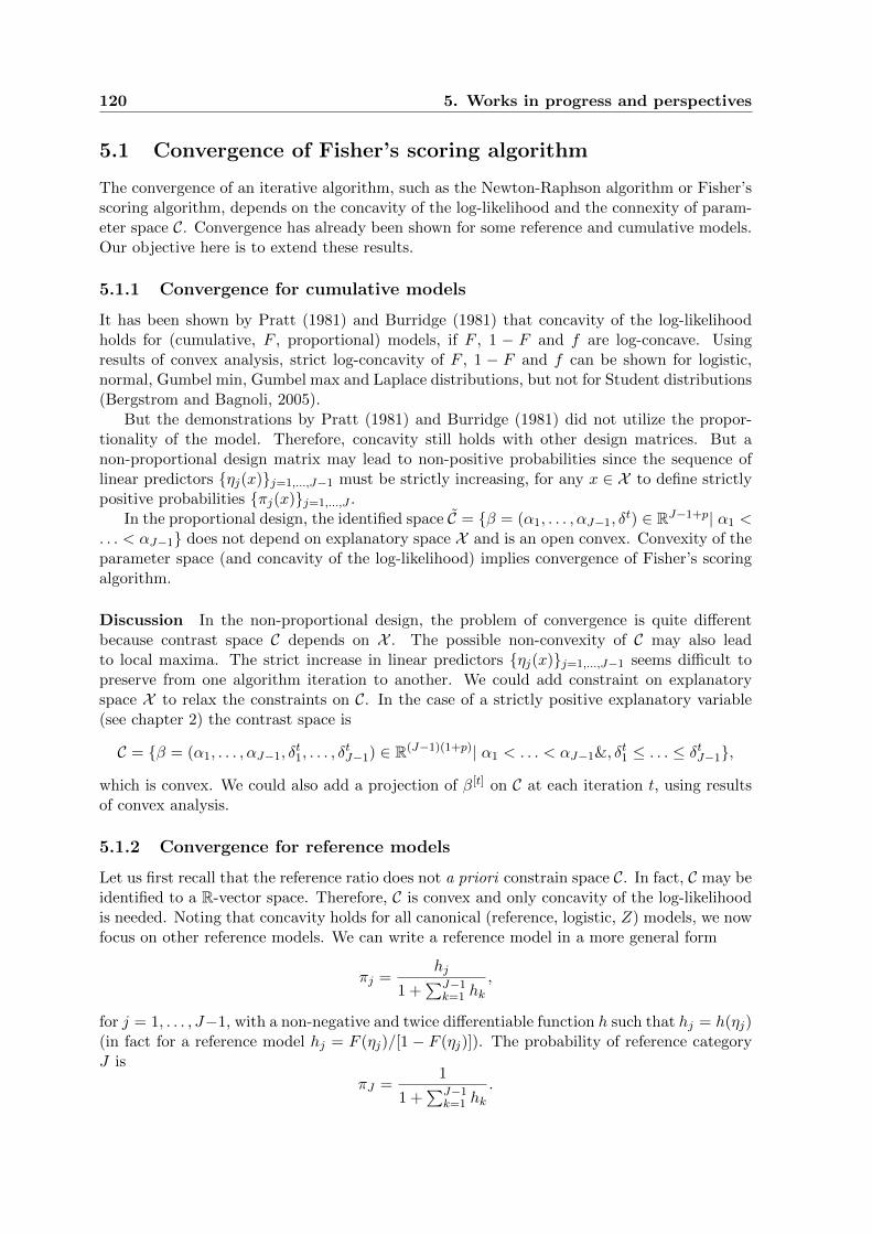
120 5. Works in progress and perspectives
5.1 Convergence of Fisher’s scoring algorithm
The convergence of an iterative algorithm, such as the Newton-Raphson algorithm or Fisher’sscoring algorithm, depends on the concavity of the log-likelihood and the connexity of param-eter space C. Convergence has already been shown for some reference and cumulative models.Our objective here is to extend these results.
5.1.1 Convergence for cumulative models
It has been shown by Pratt (1981) and Burridge (1981) that concavity of the log-likelihoodholds for (cumulative, F , proportional) models, if F , 1 − F and f are log-concave. Usingresults of convex analysis, strict log-concavity of F , 1 − F and f can be shown for logistic,normal, Gumbel min, Gumbel max and Laplace distributions, but not for Student distributions(Bergstrom and Bagnoli, 2005).
But the demonstrations by Pratt (1981) and Burridge (1981) did not utilize the propor-tionality of the model. Therefore, concavity still holds with other design matrices. But anon-proportional design matrix may lead to non-positive probabilities since the sequence oflinear predictors ηj(x)j=1,...,J−1 must be strictly increasing, for any x ∈ X to define strictlypositive probabilities πj(x)j=1,...,J .
In the proportional design, the identified space C = β = (α1, . . . , αJ−1, δt) ∈ RJ−1+p| α1 <
. . . < αJ−1 does not depend on explanatory space X and is an open convex. Convexity of theparameter space (and concavity of the log-likelihood) implies convergence of Fisher’s scoringalgorithm.
Discussion In the non-proportional design, the problem of convergence is quite differentbecause contrast space C depends on X . The possible non-convexity of C may also leadto local maxima. The strict increase in linear predictors ηj(x)j=1,...,J−1 seems difficult topreserve from one algorithm iteration to another. We could add constraint on explanatoryspace X to relax the constraints on C. In the case of a strictly positive explanatory variable(see chapter 2) the contrast space is
C = β = (α1, . . . , αJ−1, δt1, . . . , δ
tJ−1) ∈ R(J−1)(1+p)| α1 < . . . < αJ−1&, δt1 ≤ . . . ≤ δtJ−1,
which is convex. We could also add a projection of β[t] on C at each iteration t, using resultsof convex analysis.
5.1.2 Convergence for reference models
Let us first recall that the reference ratio does not a priori constrain space C. In fact, C may beidentified to a R-vector space. Therefore, C is convex and only concavity of the log-likelihoodis needed. Noting that concavity holds for all canonical (reference, logistic, Z) models, we nowfocus on other reference models. We can write a reference model in a more general form
πj =hj
1 +∑J−1
k=1 hk,
for j = 1, . . . , J−1, with a non-negative and twice differentiable function h such that hj = h(ηj)(in fact for a reference model hj = F (ηj)/[1 − F (ηj)]). The probability of reference categoryJ is
πJ =1
1 +∑J−1
k=1 hk.

5.1 Convergence of Fisher’s scoring algorithm 121
For one observation (y, x), the log-likelihood is
l =
J∑j=1
yj lnπj .
We must here recall that concavity of l with respect to β is equivalent to concavity of l withrespect to η since
∂2l
∂βt∂β= Zt
∂2l
∂ηt∂ηZ.
According to the J possible observations of y, there are only two cases: either the referencecategory is observed or not
l =
lnπJ if y = J,lnhj + lnπJ if y 6= J.
First case: y = J Here we are looking for conditions on h such that lnπJ is concave, orequivalently such that the Hessian H of − lnπJ is positive definite. The first derivative is
−∂ lnπJ∂ηj
= h′jπJ ,
for column j. The second derivative is
Hi,j = −∂2(lnπJ)
∂ηi∂ηj=∂h′j∂ηi
πJ − h′ih′jπ2J ,
for row i and column j. Differentiating the cases i = j and i 6= j we obtain
Hi,j =
h′′jπJ − h′2j π2
J , if i = j,
−h′ih′jπ2J , if i 6= j.
Again using the equality πJ = πj/hj we obtain
Hi,j =
h′′jhjπj −
h′2jh2j
π2j , if i = j,
−h′i
hi
h′jhjπiπj , if i 6= j.
Noting aj = h′′j /hj and bj = h′j/hj the Hessian matrix is
H = diagajπjj − (bibjπiπj)i,j .
whose form is similar to that of the covariance matrix
Cov(Y ) = diagπjj − (πiπj)i,j
which is positive definite. The objective is thus to find sufficient conditions on aj and bj topreserve a positive definite matrix H. Then we should rewrite these sufficient conditions interms of F (ηj), F
′(ηj) and F ′′(ηj) and obtain a differential inequality.

122 5. Works in progress and perspectives
Second case: y 6= J Assume that concavity is obtained for the first case. We simply mustshow that lnh is concave (because the sum of concave functions is concave) but this conditionis not necessary. The Hessian of lnhj is a diagonal matrix ∆ with the general term
∆j,j =h′′jhj − h′2j
h2j
.
We must show that the difference H−∆ remains positive definite, or equivalently that ∆ Hwhere denotes Loewner ordering. My intuition is that a sufficient and necessary conditionis ∆j,j < λ, where λ is the minimal eigenvalue of the matrix H.
Numerical investigation of concavity
We expect to obtain concavity of the log-likelihood for reference models if certain propertiesof cdf F are fulfilled. Meanwhile, we explored concavity numerically in the simple case J = 3(because a 3D representation can be used) using Gumbel min and max cdfs. As seen previously,we can split this into two cases.
First case: y = 3 The log-likelihood has the form
l(η1, η2) = − ln
1 +
F (η1)
1− F (η1)+
F (η2)
1− F (η2)
.
The log-likelihood shown in figure 5.1 seems to be globally concave for the two different linkfunctions.
Figure 5.1: Log-likelihood of observed reference category given (a) the (reference, Gumbelmin, Z) model and (b) the (reference, Gumbel max, Z) model.
Second case: y 6= 3 The log-likelihood has the same form for y = 1 and y = 2. Focusingonly on the case y = 1, the log-likelihood is
l(η1, η2) = ln
F (η1)
1− F (η1)
− ln
1 +
F (η1)
1− F (η1)+
F (η2)
1− F (η2)
.
The log-likelihood shown in figure 5.2 seems to be globally concave with the Gumbel max cdf,but not with the Gumbel min cdf.

5.2 Non-invariance of GLMs under permutations 123
Figure 5.2: Log-likelihood of observed non-reference category given (a) the (reference, Gumbelmin, Z) model and (b) the (reference, Gumbel max, Z) model.
Discussion Finally, the demonstration of Fisher’s scoring algorithm convergence for (cu-mulative, F , Z) models, with non proportional design matrix Z, is based on convex analysisresults whereas that of convergence for (reference, F , Z) models, with non logistic cdf F , isbased on linear algebra results.
5.2 Non-invariance of GLMs under permutations
In chapter 2 we showed the invariance of certain GLMs under particular permutations. Butare these models still invariant under other permutations?
This question is illustrated using the (reference, F , complete) and (reference, F , propor-tional) models. They are invariant under the (J − 1)! permutations that fix the referencecategory (Property 9). But are they still invariant under other permutations? Invarianceunder a permutation is easier to show than the contrary. The canonical (reference, logistic,complete) model is invariant under all permutations unlike other canonical models (reference,logistic, Z); Z ∈ Z\Zc. But a non identical transposition τ of J simply changes the designmatrix of a canonical model
(reference, logistic, Z)τ = (reference, logistic, BτZ).
Hence, the canonical link function (reference, logistic) is invariant under all permutations. Butwhat about other link functions (reference, F ) when F is not the logistic cdf? Non-invarianceof models may be shown when F is analytically defined.
Property 16. Let σ be a permutation of 1, . . . , J, F ∈ Gumbel min, Gumbel max, expo-nential and let Z be a design matrix depending on x. The (reference, F , Z) model is invariantunder σ if and only if σ(J) = J .
Proof. We have already shown that σ(J) = J is a sufficient condition for the invariance ofreference models under σ. Now we must show the necessity of this condition. Let τ be anon identical transposition of the reference category J and F ∈ Gumbel min, Gumbel max,exponential. Using a reductio ad absurdum, assume that the (reference, F , Z) model isinvariant under τ or equivalently that
(reference, F, Z)τ ⇔ (reference, F, Z).
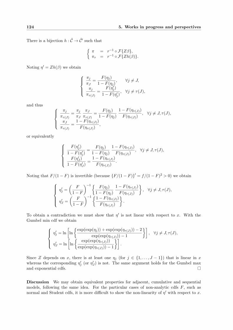
124 5. Works in progress and perspectives
There is a bijection h : C → C′ such thatπ = r−1 FZβ,πτ = r−1 FZh(β).
Noting η′ = Zh(β) we obtainπjπJ
=F (ηj)
1− F (ηj), ∀j 6= J,
πjπτ(J)
=F (η′j)
1− F (η′j), ∀j 6= τ(J),
and thus πjπτ(J)
=πjπJ
πJπτ(J)
=F (ηj)
1− F (ηj)
1− F (ητ(J))
F (ητ(J)), ∀j 6= J, τ(J),
πJπτ(J)
=1− F (ητ(J))
F (ητ(J)),
or equivalently F (η′j)
1− F (η′j)=
F (ηj)
1− F (ηj)
1− F (ητ(J))
F (ητ(J)), ∀j 6= J, τ(J),
F (η′J)
1− F (η′J)=
1− F (ητ(J))
F (ητ(J)).
Noting that F/(1− F ) is invertible (because F/(1− F )′ = f/(1− F )2 > 0) we obtainη′j =
(F
1− F
)−1 F (ηj)
1− F (ηj)
1− F (ητ(J))
F (ητ(J))
, ∀j 6= J, τ(J),
η′J =
(F
1− F
)−11− F (ητ(J))
F (ητ(J))
.
To obtain a contradiction we must show that η′ is not linear with respect to x. With theGumbel min cdf we obtain
η′j = ln
[ln
exp(exp(ηj)) + exp(exp(ητ(J)))− 2
exp(exp(ητ(J)))− 1
], ∀j 6= J, τ(J),
η′J = ln
[ln
exp(exp(ητ(J)))
exp(exp(ητ(J)))− 1
].
Since Z depends on x, there is at least one ηj (for j ∈ 1, . . . , J − 1) that is linear in xwhereas the corresponding η′j (or η′J) is not. The same argument holds for the Gumbel maxand exponential cdfs.
Discussion We may obtain equivalent properties for adjacent, cumulative and sequentialmodels, following the same idea. For the particular cases of non-analytic cdfs F , such asnormal and Student cdfs, it is more difficult to show the non-linearity of η′ with respect to x.
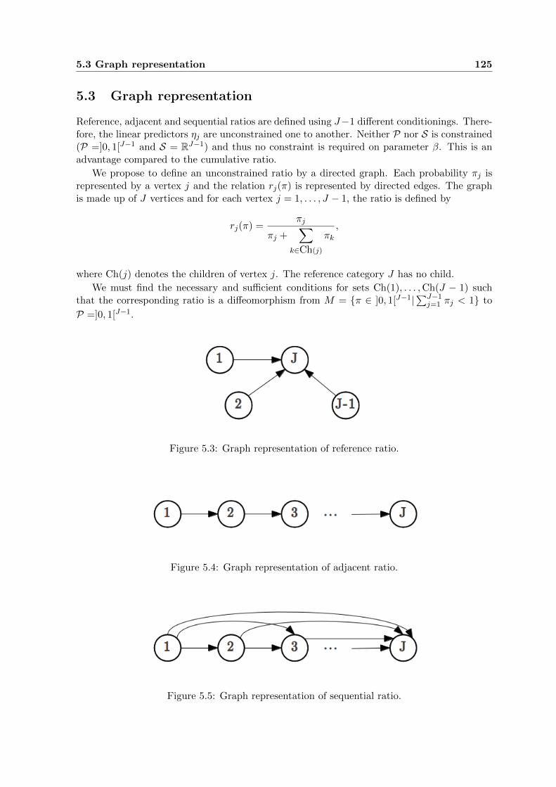
5.3 Graph representation 125
5.3 Graph representation
Reference, adjacent and sequential ratios are defined using J−1 different conditionings. There-fore, the linear predictors ηj are unconstrained one to another. Neither P nor S is constrained(P =]0, 1[J−1 and S = RJ−1) and thus no constraint is required on parameter β. This is anadvantage compared to the cumulative ratio.
We propose to define an unconstrained ratio by a directed graph. Each probability πj isrepresented by a vertex j and the relation rj(π) is represented by directed edges. The graphis made up of J vertices and for each vertex j = 1, . . . , J − 1, the ratio is defined by
rj(π) =πj
πj +∑
k∈Ch(j)
πk,
where Ch(j) denotes the children of vertex j. The reference category J has no child.
We must find the necessary and sufficient conditions for sets Ch(1), . . . ,Ch(J − 1) suchthat the corresponding ratio is a diffeomorphism from M = π ∈ ]0, 1[J−1|
∑J−1j=1 πj < 1 to
P =]0, 1[J−1.
Figure 5.3: Graph representation of reference ratio.
Figure 5.4: Graph representation of adjacent ratio.
Figure 5.5: Graph representation of sequential ratio.
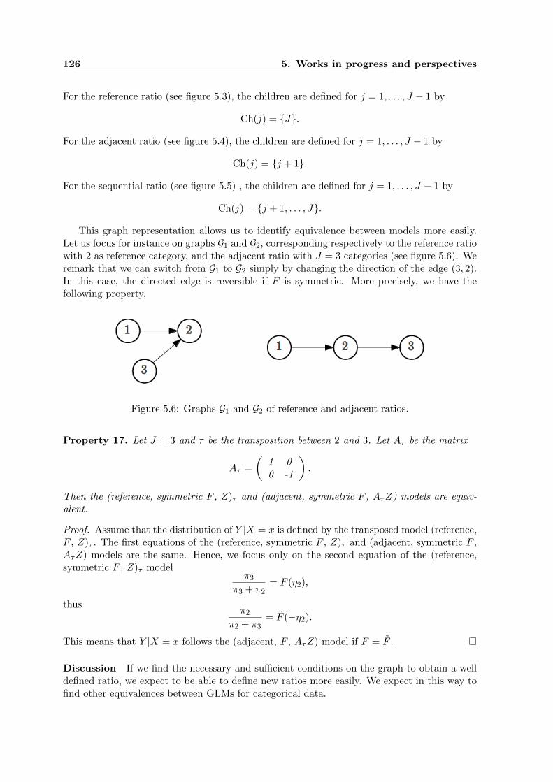
126 5. Works in progress and perspectives
For the reference ratio (see figure 5.3), the children are defined for j = 1, . . . , J − 1 by
Ch(j) = J.
For the adjacent ratio (see figure 5.4), the children are defined for j = 1, . . . , J − 1 by
Ch(j) = j + 1.
For the sequential ratio (see figure 5.5) , the children are defined for j = 1, . . . , J − 1 by
Ch(j) = j + 1, . . . , J.
This graph representation allows us to identify equivalence between models more easily.Let us focus for instance on graphs G1 and G2, corresponding respectively to the reference ratiowith 2 as reference category, and the adjacent ratio with J = 3 categories (see figure 5.6). Weremark that we can switch from G1 to G2 simply by changing the direction of the edge (3, 2).In this case, the directed edge is reversible if F is symmetric. More precisely, we have thefollowing property.
Figure 5.6: Graphs G1 and G2 of reference and adjacent ratios.
Property 17. Let J = 3 and τ be the transposition between 2 and 3. Let Aτ be the matrix
Aτ =
(1 00 -1
).
Then the (reference, symmetric F , Z)τ and (adjacent, symmetric F , AτZ) models are equiv-alent.
Proof. Assume that the distribution of Y |X = x is defined by the transposed model (reference,F , Z)τ . The first equations of the (reference, symmetric F , Z)τ and (adjacent, symmetric F ,AτZ) models are the same. Hence, we focus only on the second equation of the (reference,symmetric F , Z)τ model
π3
π3 + π2= F (η2),
thusπ2
π2 + π3= F (−η2).
This means that Y |X = x follows the (adjacent, F , AτZ) model if F = F .
Discussion If we find the necessary and sufficient conditions on the graph to obtain a welldefined ratio, we expect to be able to define new ratios more easily. We expect in this way tofind other equivalences between GLMs for categorical data.

5.4 Qualitative choice models 127
5.4 Qualitative choice models
In this framework, statistical unit i is a consumer, J categories are different alternatives andx are attributes influencing the consumer’s choice. In this section we first present a number ofqualitative choice models using a classical predictive approach, then propose to extend thesemodels using the (r, F, Z) specification.
5.4.1 Classical approach
5.4.1.1 Model specification
We saw in chapter 1 that Luce’s choice axiom Luce (1959) and the principle of random utilitymaximisation lead to the model
P (Y = j) =exp(ηj)
1 +∑J−1
k=1 exp(ηk)(5.1)
for j = 1, . . . , J − 1. Depending on the form of the linear predictors ηj , we obtain differentlogit models:
• Multinomial logit model: ηj = αj +xtδj . The attributes are common for all alternativesand the parameters depend on each alternative.
• Conditional logit model: ηj = α + xtjδ. The attributes depend on each alternative andthe parameters are common for all alternatives.
• Universal logit model: ηj = αj + xtjδj . The attributes and the parameters depend oneach alternative.
5.4.1.2 Independence of irrelevant alternatives
Since these three logit models satisfy Luce’s choice axiom, they share the IIA property. Theratio of probabilities for alternatives j and k
P (Y = j)
P (Y = k)= exp(ηj − ηk)
does not depend on other alternatives. As noted by McFadden (1986), “the IIA axiom is ablessing and a curse”. On the negative side, it is inconsistent with the heterogeneous patternsof similarities often encountered in economics and marketing problems. This is well illustratedby Marschak (1960) through the blue/red bus example. On the positive side, “it makesforecasting the demand for a new alternative an easy calculation” (McFadden, 1986).
5.4.1.3 Prediction for a new alternative
In the econometrics framework, qualitative choice regression models are often used in a predic-tive manner. With the multinomial logit model, the probability of each alternative P (Y = j|x)can be predicted for any value x which is not observed in the dataset. For the conditionallogit model (McFadden, 1974), the situation is quite different because linear predictors havea different form: ηj = α + xtjδ. Here, the attribute value xj is related to the alternative j,which is why the model is called the conditional logit model. The probability P (Y = 0|x0) ofa new alternative 0 can be predicted because the intercept α and the slope δ are common forall alternatives.
128 5. Works in progress and perspectives
Let us illustrate the predictive approach using the classical situation of urban travel de-mand. The consumer has J = 3 alternatives: car, bus or bicycle. He makes a decisionaccording to travel cost c and travel time t. It should be noted that these two attributes arequantitative and are related to the different alternatives: cj and tj are travel cost and traveltime of alternative j. The conditional logit model may be summarized by
P (Y = j) =exp(α+ xtjδ)
1 +∑J−1
k=1 exp(α+ xtkδ),
where xj = xj − xJ for j = 1, . . . , J − 1. For urban travel demand, we obtain
P (Y = j) =exp(α+ ctjδ1 + ttjδ2)
1 +∑2
k=1 exp(α+ ctkδ1 + ttkδ2),
where cj = cj − cJ , tj = tj − tJ , for j = 1, 2. The estimated parameter β = (α, δ) is obtainedby likelihood maximisation, using Fisher’s scoring algorithm.
Now, imagine that the construction of a tram system is planned. The probability of eachindividual using it can be predicted to assess the resident’s demand. Since the tram system(new alternative 0) does not exist, the attributes values c0 and t0 are not yet available. Theymust therefore be simulated or estimated using observed data in another city where a tramis already used. Let c0, t0 be the corresponding values and c0, t0 the translated values withrespect to the reference alternative c0 = c0 − c3, t0 = t0 − t3. The predicted probability ofchoosing the tramway is
P (Y = 0) =exp(α+ ct0δ1 + tt0δ2)
1 +∑2
k=0 exp(α+ ctkδ1 + ttkδ2).
More generally, the predicted probability of choosing the new alternative 0 is
P (Y = 0) =exp(α+ xt0δ)
1 +∑J−1
k=0 exp(α+ xtkδ).
It should be noted that adding the new alternative 0 does not change the ratio of proba-bilities πj/πk of other alternatives j, k because of the IIA property. For example, the numberof bus users is still three times the number of bicycle users after construction of the tramsystem. But the new alternative needs to be different from other alternatives (reminiscent ofthe blue/red bus paradox).
5.4.2 (r,F,Z) approach
5.4.2.1 Model specification
Qualitative choice models of form (5.1) are exactly canonical (reference, logistic, Z) models.The three previously mentioned logit models correspond to different forms of the design matrixZ:
• Multinomial logit model: Z = Zc with
Zc =
1 xt
. . .. . .
1 xt
.
This is the complete design matrix.
5.4 Qualitative choice models 129
• Conditional logit model: Z = Z with
Z =
1 xt1...
...1 xtJ−1
,
where xj = xj − xJ (translation with respect to reference category J).
• Universal logit model: Z = Zc with
Zc =
1 xt1. . .
. . .
1 xtJ−1
.
These three types of qualitative choice models can be easily extended using other cdfs F . Theyare useful for qualitative choices, especially because of the reference ratio. Also the referencecategory can be changed (with a transposition τ) to obtain a better fit (changing also thetranslated variables xj = xj − xτ(J) for j 6= τ(J)).
5.4.2.2 Independence of irrelevant alternatives
Property 18. All the reference models share the IIA property.
Proof. All the reference models have the form (reference, F , Z)τ , where τ is a transpositionof the reference category J . Without loss of generality, we simply consider the case of thereference category J (i.e. τ is the identical transposition). Assume that the distribution ofY |X = x is defined by a reference model
πjπj + πJ
= F (ηj), j = 1, ..., J − 1,
⇔ πj =F (ηj)
1− F (ηj)πJ , j = 1, ..., J − 1.
Thus, for two alternatives j, k ∈ 1, ..., J − 1
πjπk
=F (ηj)/[1− F (ηj)]
F (ηk)/[1− F (ηk)],
andπjπJ
= F (ηj)/[1− F (ηj)].
Finally, the ratio of probabilities of two alternatives πj/πk does not depend on other alterna-tives.
In fact, the IIA property is related to the ratio, not the logistic cdf of the multinomiallogit model. By contrast, the adjacent, cumulative and sequential models do not share theIIA property because they use the category ordering assumption (see Appendix D for details).It should be noted that the situation of new alternative is not easily interpretable for orderedalternatives.
130 5. Works in progress and perspectives
5.4.2.3 Prediction for a new alternative
We propose to extend the conditional logit model specified by the (reference, logistic, Z) tripletto (reference, F , Z) models
P (Y = j) =F (α+ xtjδ)/(1− F (α+ xtjδ))
1 +∑J−1
k=1 F (α+ xtkδ)/(1− F (α+ xtkδ)),
for j = 1, . . . , J − 1. The cdf F must first be selected using error of misclassification or log-likelihood criteria. The log-likelihood does not need to be penalized because all the proposedmodels have the same design matrix and thus the same number of parameters 1 + p. Aftera comparison with classical cdfs (logistic, normal, Laplace, Gumbel min, Gumbel max andStudent(d)), the best model is obtained with cdf F and parameters β = (α, δ). The predictedprobability of a new alternative 0 is
P (Y = 0) =F (α+ xt0δ)/(1− F (α+ xt0δ))
1 +∑J−1
k=0 F (α+ xtkδ)/(1− F (α+ xtkδ)).
Furthermore the reference alternative can be changed to obtain a better fit. The best modelis obtained with cdf F , reference alternative j and parameters β = (α, δ). In this case thepredicted probability of a new alternative 0 is
P (Y = 0) =F (α+ xt0δ)/(1− F (α+ xt0δ))
1 +∑J
k=0,k 6=j F (α+ xtkδ)/(1− F (α+ xtkδ)),
where xj = xj − xj for j 6= j.
Discussion The theoretical work conducted on this perspective has almost been completedbut remains questionable. On the one hand, the proposed qualitative choice models do notrespect the principle of random utility maximisation. On the other hand, does a better fit ora smallest error of misclassification mean better predictions?
With regard to applications, the proposed qualitative choice models could be estimatedusing benchmark datasets and could be compared with the conditional logit model. Ideally,we would like to obtain the real observed proportions of the new alternatives and comparepredicted and true values. For Fisher’s scoring algorithm, only the design matrix has to bemodified. But the explanatory variables x = xjj=1,...,J must be considered with dependencieson alternatives.
Appendix A
Proof of Property 4
The following proof is a generalisation of that described by Dobson (2002) for the multivariatecase (i.e. K > 1). From the definition of a probability density function, the area under thecurve is unity ∫
f(y, µ) dy = 1, (A.1)
where integration is over all possible values of y (if the random variable Y is discrete thenintegration is replaced by summation). If we differentiate both sides of (A.1) with respect toµ we obtain
∂
∂µ
∫f(y, µ)dy
=
∂
∂µ1 = 0K ,
where 0K is the null vector of dimension K. Assuming differentiability of functions θ and bwith respect to µ, we can apply the Leibniz integral rule and obtain∫
∂
∂µf(y, µ)dy = 0K . (A.2)
For distribution of the exponential family we have
∂
∂µf(y, µ) =
∂
∂µ
(a(y)tθ(µ) + b(µ) + c(y)
)· f(y, µ)
∂
∂µf(y, µ) = Jθ(µ)a(y) +∇b(µ) · f(y, µ) (A.3)
Therefore (A.2) becomes∫Jθ(µ) ∗ a(y) +∇b(µ) · f(y, θ)dy = 0K∫
Jθ(µ) ∗ a(y) · f(y, θ)dy = −∇b(µ) ·∫f(y, θ)dy
Jθ(µ) ∗ E[a(Y )] = −∇b(µ) (A.4)
and thus the desired result (i).
A similar method can be used to obtain Var[a(Y )].
∂2
∂µt∂µ
∫f(y, µ)dy
=
∂2
∂µt∂µ· 1 = 0K×K ,
where 0K×K is the null matrix of dimension K ×K. Thus∫∂2
∂µt∂µf(y, µ) dy = 0K×K (A.5)
132 A. Proof of Property 4
Using (A.3), we obtain
∂2
∂µt∂µf(y, µ) =
∂
∂µt[Jθ(µ) ∗ a(y) +∇b(µ) · f(y, µ)]
∂2
∂µt∂µf(y, µ) =
[∂
∂µtJθ(µ) ∗ a(y) +∇b(µ)
]· f(y, µ) + Jθ(µ) ∗ a(y) +∇b(µ) ∂
∂µtf(y, µ).
Using (A.3) again, we obtain
∂2
∂µt∂µf(y, µ) =
[∂
∂µtJθ(µ) ∗ a(y) +∇b(µ)
]· f(y, µ) (A.6)
+ Jθ(µ) ∗ a(y) +∇b(µ) Jθ(µ)a(y) +∇b(µ)t · f(y, µ). (A.7)
Computation of part (A.6)
∂
∂µtJθ(µ)a(y) +∇b(µ) =
∂
∂µtJθ(µ)a(y)+Hb(µ)
=
(∂2θ
∂µj∂µi
)ta(y)
i,j
+Hb(µ).
Computation of part (A.7)
Jθ(µ)a(y) +∇b(µ) = Jθ(µ) a(y)− E[a(Y )] + E[a(Y )]+∇b(µ)
= Jθ(µ) a(y)− E[a(Y )]+ Jθ(µ) ∗ E[a(Y )] +∇b(µ)︸ ︷︷ ︸=0K according to (A.2)
.
Finally (A.3) becomes
∂2
∂µt∂µf(y, µ) =
( ∂2θ
∂µj∂µi
)ta(y)
i,j
+Hb(µ)
· f(y, µ)
+ Jθ(µ) a(y)− E[a(Y )] a(y)− E[a(Y )]t J tθ (µ).
By integrating with respect to y and using (A.5), we obtain∫ ( ∂2θ
∂µj∂µi
)ta(y)
i,j
· f(y, µ)dy
+Hb(µ)
[∫f(y, µ)dy
]︸ ︷︷ ︸
=1
+Jθ(µ)
[∫a(y)− E[a(Y )] a(y)− E[a(Y )]t · f(y, θ)dy
]︸ ︷︷ ︸
=Cov[a(Y )]
J tθ (µ) = 0K×K ,
or equivalently∫ ( ∂2θ
∂µj∂µi
)ta(y)
i,j
· f(y, µ)dy
+Hb(µ) + Jθ(µ)Cov[a(Y )]J tθ (µ) = 0K×K .
The scalar product and expectation are linear functions and we thus obtain(∂2θ
∂µj∂µi
)tE[a(y)]
i,j
+Hb(µ) + Jθ(µ)Cov[a(Y )]J tθ (µ) = 0K×K .
Finally, using the first result (i), we obtain the second result (ii).
Appendix B
Details on Fisher’s scoringalgorithm
Below are details on computation of the Jacobian matrix ∂π∂r for four different ratios.
Reference For the reference ratio we have for j = 1, . . . , J − 1
πj =rj
1− rjπJ . (B.1)
Summing on j from 1 to J − 1 we obtain
πJ =1
1 +∑J−1
j=1rj
1−rj
.
The derivative of the product (B.1) with respect to ri is
∂πj∂ri
=∂
∂ri
(rj
1− rj
)πJ +
rj1− rj
∂πJ∂ri
. (B.2)
For the term of the sum part we obtain
∂
∂ri
(rj
1− rj
)=
1
(1− ri)2if i = j,
0 otherwise.
For the second term of the sum we obtain
∂πJ∂ri
= − 1
(1− ri)2π2J .
Then (B.2) becomes
∂πj∂ri
=
1
ri(1− ri)
[ri
1− riπJ −
(ri
1− riπJ
)2]
if i = j,
− 1
ri(1− ri)ri
1− rirj
1− rjπ2J otherwise.
Using (B.1) again we obtain
∂πj∂ri
=1
ri(1− ri)
πi(1− πi) if i = j,−πiπj otherwise.
Finally we have∂πj∂ri
=Cov(Yi, Yj)
F (ηi)[1− F (ηi)],
for row i and column j of the Jacobian matrix.
134 B. Details on Fisher’s scoring algorithm
Adjacent For the adjacent ratio we have for j = 1, . . . , J − 1
πj =rj
1− rjπj+1.
and thus
πj =
J−1∏k=j
rk1− rk
πJ . (B.3)
Summing on j from 1 to J − 1 we obtain
πJ =1
1 +∑J−1
j=1
∏J−1k=j
rk1−rk
.
The derivative of the product (B.3) with respect to ri is
∂πj∂ri
=∂
∂ri
J−1∏k=j
rk1− rk
πJ +
J−1∏k=j
rk1− rk
∂πJ∂ri
. (B.4)
For the first term of the sum we obtain
∂
∂ri
J−1∏k=j
rk1− rk
=
1
ri(1− ri)
J−1∏k=j
rk1− rk
if i ≥ j,
0 otherwise.
For the second term of the sum we obtain
∂πJ∂ri
= − 1
ri(1− ri)
i∑k=1
J−1∏k=j
rk1− rk
π2J .
Using (B.3) it becomes
∂πJ∂ri
= − πJri(1− ri)
i∑k=1
πk.
Then (B.4) becomes
∂πj∂ri
=
1
ri(1− ri)
(πj − πj
i∑k=1
πk
)if i ≥ j,
− 1
ri(1− ri)πj
i∑k=1
πk otherwise.
Finally we have∂πj∂ri
=1
F (ηi)[1− F (ηi)]
πj(1− γi) if i ≥ j,−πjγi otherwise,
for row i and column j of the Jacobian matrix, where γi = P (Y ≤ i) =∑i
k=1 πk.
135
Sequential For the sequential ratio we have for j = 1, . . . , J − 1
πj = rj
j−1∏k=1
(1− rk),
with the convention∏0k=1(1− rk) = 1. Hence we obtain directly
∂πj∂ri
=
j−1∏k=1
1− F (ηk) if i = j,
−F (ηj)
j−1∏k=1,k 6=i
1− F (ηk) if i < j,
0 otherwise,
for row i and column j of the Jacobian matrix.
Cumulative For the cumulative ratio we have for j = 1, . . . , J − 1
πj = rj − rj−1,
with the convention r0 = 0. Hence we obtain directly
∂π
∂r=
1 −1
1. . .. . . −1
1
.

136 B. Details on Fisher’s scoring algorithm
Appendix C
Details on SMS-PCGLM
Definition of hidden semi-Markov chains (HSMCs) and of semi-Markov switching partitioned conditional generalized linear mod-els (SMS-PCGLMs) and associated statistical methods
Semi-Markov chain
Let St be a semi-Markov chain with finite-state space 0, . . . , A − 1. This A-state semi-Markov chain St is defined by the following parameters:
• initial probabilities ϕa = P (S0 = a) with∑
a ϕa = 1.
• transition probabilities
– non absorbing state a: ∀b 6= a, pa,b = P (St = b|St 6= a, St−1 = a) with∑
b 6=a pa,b = 1and pa,a = 0,
– absorbing state a: pa,a = P (St = a|St−1 = a) = 1 and ∀b 6= a, pa,b = 0.
An explicit occupancy (or sojourn time) distribution is attached to each non absorbing statea:
da(u) = P (St+u+1 6= a, St+u−v = a, v = 0, . . . , u− 2|St+1 = a, St 6= a), u = 1, 2, . . .
Since t = 0 is assumed to correspond to a state entering, the following relation is verified
P (St 6= a, St−v = a, v = 1, . . . , t) = da(t)ϕa.
We define as possible parametric state occupancy distributions binomial distributions, Poissondistributions and negative binomial distributions with an additional shift parameter d (d ≥ 1)which defines the minimum sojourn time in a given state.
The binomial distribution with parameters d, n and p (q = 1 − p), B(d, n, p) where 0 ≤p ≤ 1, is defined by
da(u) =
(n− du− d
)pu−dqn−u, u = d, d+ 1, . . . , n,
with µ = d+ (n− d)p and σ2 = (n− d)pq.
The Poisson distribution with parameters d and λ, P(d, λ), where λ is a real number(λ > 0), is defined by
da(u) =exp(−λ)λu−d
(u− d)!, u = d, d+ 1, . . .
with µ = d+ λ and σ2 = λ.
138 C. Details on SMS-PCGLM
The negative binomial distribution with parameters d, r and p, NB(d, r, p), where r is areal number (r > 0) and 0 < p ≤ 1, is defined by
da(u) =
(u− d+ r − 1
r − 1
)prqu−d, u = d, d+ 1, . . .
with µ = d+ rq/p and σ2 = rq/p2.
Partitioned conditional generalized linear models for categorical responsevariables
A PCGLM is defined by a partition tree of categories 1, . . . , J and by a triplet specifyingthe GLM associated with each non-terminal node of the partition tree:
• Ratio of category probabilities i.e. reference ratio for non-ordered subset of categoriesdefined by πj/(πj + πJ) for the reference category J (πj is the probability of categoryj), adjacent, sequential and cumulative ratios for ordered subset of categories definedrespectively by πj/(πj + πj+1), πj/(πj + . . .+ πJ) and π1 + . . .+ πj .
• Cumulative distribution function of a continuous distribution (e.g. symmetric distribu-tions such as the logistic, Gaussian or Student distributions, or non-symmetric distribu-tions such as the Gumbel min or max distributions) whose inverse defined the mappingbetween the category probability ratios and the linear predictor.
• Design matrix for the parameterization of the linear predictor.
Hidden semi-Markov chains
A hidden semi-Markov chain can be viewed as a pair of stochastic processes St, Yt wherethe “output” process Yt is related to the “state” process St, which is a finite-state semi-Markov chain, by a probabilistic function or mapping denoted by f (hence Yt = f(St)). Sincethe mapping f is such that a given output may be observed in different states, the stateprocess St is not observable directly but only indirectly through the output process Yt.This output process Yt is related to the semi-Markov chain St by the observation (oremission) probabilities ba(y) = P (Yt = y|St = a). The definition of observation probabilitiesexpresses the assumption that the output process at time t depends only on the underlyingsemi-Markov chain at time t. In the case of a categorical observed variable such as thetypes of axillary productions, the observation probabilities are directly estimated (categoricalobservation distribution). In the case of a quantitative observed variable such as the internodelength, discrete parametric observation distributions are estimated (in this context, binomial,Poisson or negative binomial distributions may be unshifted). In the multivariate case, theelementary observed variables at time t are assumed to be conditionally independent given thestate St = st.
Semi-Markov switching partitioned conditional generalized linear models
Compared to a simple HSMC, the difference concerns the output process Yt which is nowmodulated by explanatory variables Xt that vary with the index parameter (in our casenode rank). Observation distributions are thus replaced by regression models, in our case byPCGLMs, but the conditional independence assumption between state and output processesis unchanged.

139
Statistical methods and algorithms for hidden semi-Markov chains and semi-Markov switching partitioned conditional generalized linear models
The maximum likelihood estimation of the parameters of a HSMC requires an iterative opti-mization technique, which is an application of the expectation-maximization (EM) algorithm.The maximum likelihood estimation of the parameters of a SMS-PCGLM requires a variant ofthe EM algorithm called the gradient EM algorithm. Compared to the estimation of hiddensemi-Markov chains using the simple EM algorithm, the main difference concerns the M-stepof the algorithm where the direct maximization of observation distributions is replaced by theiterative Fisher’s scoring algorithm.
Once a HSMC or a SMS-PCGLM has been estimated, the most probable state sequence s∗
with its associated posterior probability P (S = s∗|Y = y) can be computed for each observedsequence y using the so-called Viterbi algorithm. In our application context, the most probablestate sequence can be interpreted as the optimal segmentation of the corresponding observedsequence in successive branching zones; see Guedon (2003, 2005); Guedon et al. (2007) forstatistical methods for hidden semi-Markov chains (with exception of the iterative M-step forthe estimation, all the other statistical methods and algorithms for HSMCs directly apply toSMS-PCGLM).

140 C. Details on SMS-PCGLM
Appendix D
Details on IIA property
All the reference models share the IIA property. By contrast we show that adjacent, sequentialand cumulative models do not share this property because they are defined using the categoryordering assumption.
Adjacent For adjacent models we have
πjπj + πj+1
= F (ηj), ∀j ∈ 1, . . . , J − 1,
or equivalently
πj =F (ηj)
1− F (ηj)πj+1, ∀j ∈ 1, . . . , J − 1.
Thus for j, k ∈ 1, . . . , J with j < k we have
πjπk
=k−1∏m=j
F (ηm)
1− F (ηm).
Finally the ratio of probabilities of two alternatives πj/πk depends on intermediate alternatives.
Sequential For sequential models we haveπj
πj + . . .+ πJ= F (ηj), ∀j ∈ 1, . . . , J − 1,
or equivalently
πj = F (ηj)
j−1∏k=1
[1− F (ηk)], ∀j ∈ 1, . . . , J − 1.
Then for j, k ∈ 1, . . . , J with j > k we have
πjπk
=F (ηj)
F (ηk)
j−1∏m=k
[1− F (ηm)],
with the convention ηJ = ∞. Finally, the ratio of probabilities of two alternatives πj/πkdepends on intermediate alternatives.
Cumulative For cumulative models we have
π1 + . . .+ πj = F (ηj), ∀j ∈ 1, . . . , J − 1,
or equivalentlyπj = F (ηj)− F (ηj−1), ∀j ∈ 1, . . . , J,
using the convention η0 = −∞ and ηJ =∞. Then for j, k ∈ 1, . . . , J with j 6= k we have
πjπk
=F (ηj)− F (ηj−1)
F (ηk)− F (ηj−k).


Bibliography
A. Agresti. Categorical data analysis, volume 359. John Wiley and Sons, 2002. 7, 9, 19, 36,56, 59, 83
A. Agresti. Analysis of ordinal categorical data, volume 656. Wiley, 2010. 7, 9, 10, 19, 39, 43,56, 68, 69
R. M. K. Altman. Mixed hidden markov models. Journal of the American Statistical Associ-ation, 102(477):201–210, 2007. 52
J. A. Anderson. Regression and ordered categorical variables. Journal of the Royal StatisticalSociety. Series B (Methodological), pages 1–30, 1984. 8, 11, 20, 21, 39, 44, 45, 82, 92, 98
D. Barthelemy and Y. Caraglio. Plant architecture: a dynamic, multilevel and comprehensiveapproach to plant form, structure and ontogeny. Annals of Botany, 99(3):375–407, 2007. 24
T. Bergstrom and M. Bagnoli. Log-concave probability and its applications. Economic theory,26:445–469, 2005. 33, 40, 120
J. Burridge. A note on maximum likelihood estimation for regression models using groupeddata. Journal of the Royal Statistical Society. Series B (Methodological), pages 41–45, 1981.40, 120
F. Chaubert-Pereira, Y. Caraglio, C. Lavergne, and Y. Guedon. Identifying ontogenetic,environmental and individual components of forest tree growth. Annals of botany, 104(5):883–896, 2009. 11, 106, 116, 117
G. A. Churchill. Stochastic models for heterogeneous dna sequences. Bulletin of mathematicalbiology, 51(1):79–94, 1989. 51
I. B. Collings and T. Ryden. A new maximum likelihood gradient algorithm for on-line hiddenmarkov model identification. In Acoustics, Speech and Signal Processing, 1998. Proceedingsof the 1998 IEEE International Conference on, volume 4, pages 2261–2264. IEEE, 1998. 52
D. R. Cox. Regression models and life-tables. Journal of the Royal Statistical Society. SeriesB (Methodological), pages 187–220, 1972. 41
G. Debreu. Review of rd luce, individual choice behavior: A theoretical analysis. AmericanEconomic Review, 50(1):186–188, 1960. 38, 46, 88
A. P. Dempster, N. M. Laird, and D. B. Rubin. Maximum likelihood from incomplete datavia the em algorithm. Journal of the Royal Statistical Society. Series B (Methodological),pages 1–38, 1977. 52
A. J. Dobson. An introduction to generalized linear models. CRC Pr I Llc, 2002. 9, 19, 27, 29,34, 56, 131
D. M. Doran and D. J. Newell. Manipulation in treatment of low back pain: a multicentrestudy. British Medical Journal, 2(5964):161, 1975. 47, 91, 98
144 Bibliography
L. Fahrmeir and G. Tutz. Multivariate statistical modelling based on generalized linear models.Springer Verlag, 2001. 7, 19, 36, 58, 83
J. D. Ferguson. Variable duration models for speech. In Proc. Symposium on the applicationof hidden Markov models to text and speech, pages 143–179, 1980. 51
S. Fruhwirth-Schnatter. Finite mixture and Markov switching models. 2006. 107
L. E. Gatsuk, O. V. Smirnova, L. I. Vorontzova, L. B. Zaugolnova, and L. A. Zhukova. Agestates of plants of various growth forms: a review. The Journal of Ecology, pages 675–696,1980. 8, 19, 116
C. Godin and Y. Caraglio. A multiscale model of plant topological structures. Journal oftheoretical biology, 191(1):1–46, 1998. 24
Y. Guedon. Review of several stochastic speech unit models. Computer Speech & Language,6(4):377–402, 1992. 51
Y. Guedon. Estimating hidden semi-markov chains from discrete sequences. Journal of Com-putational and Graphical Statistics, 12(3):604–639, 2003. 50, 53, 139
Y. Guedon. Hidden hybrid markov/semi-markov chains. Computational statistics & Dataanalysis, 49(3):663–688, 2005. 139
Y. Guedon and C. Cocozza-Thivent. Explicit state occupancy modelling by hidden semi-markov models: application of derin’s scheme. Computer Speech & Language, 4(2):167–192,1990. 53
Y. Guedon, D. Barthelemy, Y. Caraglio, and E. Costes. Pattern analysis in branching andaxillary flowering sequences. Journal of theoretical biology, 212(4):481–520, 2001. 11, 20, 24,25, 106
Y. Guedon, Y. Caraglio, P. Heuret, E. Lebarbier, and C. Meredieu. Analysing growth compo-nents in trees. Journal of Theorical Biology, pages 418–447, 2007. 139
H-H. Han, C. Coutand, H. Cochard, C. Trottier, and P-E. Lauri. Effects of shoot bendingon lateral fate and hydraulics: invariant and changing traits across five apple genotypes.Journal of experimental botany, 58(13):3537–3547, 2007. 11, 106
T. Hastie, R. Tibshirani, J. Friedman, and J. Franklin. The elements of statistical learning:data mining, inference and prediction. The Mathematical Intelligencer, 27(2):83–85, 2005.75
P. Heuret, D. Barthelemy, Y. Guedon, X. Coulmier, and J. Tancre. Synchronization of growth,branching and flowering processes in the south american tropical tree cecropia obtusa (ce-cropiaceae). American Journal of Botany, 89(7):1180–1187, 2002. 24
Baillaud L. Structures repetitives spatiales et spatio-temporelles des plantes. Phytomorphology,49:377–404, 1999. 24
E. Laara and J. N. S. Matthews. The equivalence of two models for ordinal data. Biometrika,72(1):206–207, 1985. 10, 42, 56, 66, 72
Bibliography 145
P-E. Lauri and E. Terouanne. The influence of shoot growth on the pattern of axillary de-velopment on the long shoots of young apple trees (malus domestica borkh.). Internationaljournal of plant sciences, pages 283–296, 1998. 11, 25, 106
S. E. Levinson. Continuously variable duration hidden markov models for automatic speechrecognition. Computer Speech & Language, 1(1):29–45, 1986. 51
T-S. Lim, W-Y. Loh, and Y-S. Shih. A comparison of prediction accuracy, complexity, andtraining time of thirty-three old and new classification algorithms. Machine learning, 40(3):203–228, 2000. 75
R. D. Luce. Individual choice behavior. 1959. 7, 9, 19, 37, 56, 127
J. Marschak. Binary-choice constraints and random utility indicators. In Proceedings of aSymposium on Mathematical Methods in the Social Sciences, 1960. 7, 19, 38, 127
G. N. Masters. A rasch model for partial credit scoring. Psychometrika, 47(2):149–174, 1982.7, 9, 19, 56
A. E. Maxwell. Analysing qualitative data. Methuen London, 1961. 73
P. McCullagh. A class of parametric models for the analysis of square contingency tables withordered categories. Biometrika, 65(2):413–418, 1978. 10, 56, 69
P. McCullagh. Regression models for ordinal data. Journal of the Royal Statistical Society.Series B (Methodological), pages 109–142, 1980. 7, 9, 19, 39, 56, 61, 71, 73
D. McFadden. Conditional logit analysis of qualitative choice behavior. 1973. 7, 19, 21, 38
D. McFadden. Conditional logit analysis of qualitative choice analysis. Frontiers in Econo-metrics, pages 105–142, 1974. 12, 47, 89, 119, 127
D. McFadden. The choice theory approach to market research. Marketing science, 5(4):275–297, 1986. 127
D. McFadden et al. Modelling the choice of residential location. Institute of TransportationStudies, University of California, 1978. 7, 10, 19, 20, 45, 46, 81, 82, 85, 88, 90
B. Morawitz and G. Tutz. Alternative parameterizations in business tendency surveys. Math-ematical Methods of Operations Research, 34(2):143–156, 1990. 10, 82
J. A. Nelder and R. W. M. Wedderburn. Generalized linear models. Journal of the RoyalStatistical Society. Series A (General), pages 370–384, 1972. 7, 9, 19, 27, 28, 56
E. Nicolini, B. Chanson, and F. Bonne. Stem growth and epicormic branch formation inunderstorey beech trees (fagus sylvatica l.). Annals of Botany, 87(6):737–750, 2001. 26
J. Peyhardi, E. Costes, Y. Caraglio, P-E. Lauri, C. Trottier, and Y. Guedon. Integrativemodels for analyzing jointly shoot growth and branching patterns. In 7th InternationalWorkshop on Functional Structural Plant Models, 2013a. 117
J. Peyhardi, C. Trottier, and Y. Guedon. A unifying framework for specifying generalizedlinear models for categorical data. In 28th International Workshop on Statistical Modeling,2013b. 108, 116
146 Bibliography
J. W. Pratt. Concavity of the log likelihood. Journal of the American Statistical Association,76(373):103–106, 1981. 40, 120
L. R. Rabiner. A tutorial on hidden markov models and selected applications in speechrecognition. Proceedings of the IEEE, 77(2):257–286, 1989. 51, 52
M. Renton, Guedon Y., C. Godin, and E. Costes. Similarities and gradients in growth unitbranching patterns during ontogeny in ‘fuji’apple trees: a stochastic approach. Journal ofExperimental Botany, 57(12):3131–3143, 2006. 11, 25, 106, 108
M. Russell and R. Moore. Explicit modelling of state occupancy in hidden markov mod-els for automatic speech recognition. In Acoustics, Speech, and Signal Processing, IEEEInternational Conference on ICASSP’85., volume 10, pages 5–8. IEEE, 1985. 51, 52
T. A. Steeves and I. M. Sussex. Patterns in plant development. Cambridge University Press,1989. 8, 19
O. Taugourdeau, F. Chaubert-Pereira, S. Sabatier, and Y. Guedon. Deciphering the devel-opmental plasticity of walnut saplings in relation to climatic factors and light environment.Journal of experimental botany, 62(15):5283–5296, 2011. 116
R. Turner. Direct maximization of the likelihood of a hidden markov model. ComputationalStatistics & Data Analysis, 52(9):4147–4160, 2008. 52
G. Tutz. Compound regression models for ordered categorical data. Biometrical Journal, 31(3):259–272, 1989. 10, 20, 45, 47, 48, 82, 85, 90
G. Tutz. Sequential item response models with an ordered response. British Journal ofMathematical and Statistical Psychology, 43(1):39–55, 1990. 7, 9, 19, 56, 61
G. Tutz. Sequential models in categorical regression. Computational Statistics & Data Anal-ysis, 11(3):275–295, 1991. 10, 41, 42, 56, 60, 66, 68
G. Tutz. Regression for categorical data, volume 34. Cambridge University Press, 2012. 7, 19,45, 59, 83, 100, 102
R. W. M. Wedderburn. On the existence and uniqueness of the maximum likelihood estimatesfor certain generalized linear models. Biometrika, 63(1):27–32, 1976. 33
J. White. The plant as a metapopulation. Annual Review of Ecology and Systematics, 10:109–145, 1979. 24
Q. Zhang and E. H. Ip. Generalized linear model for partially ordered data. Statistics inMedicine, 2012. 7, 10, 19, 20, 45, 46, 49, 82, 85, 86, 95, 96, 98, 100


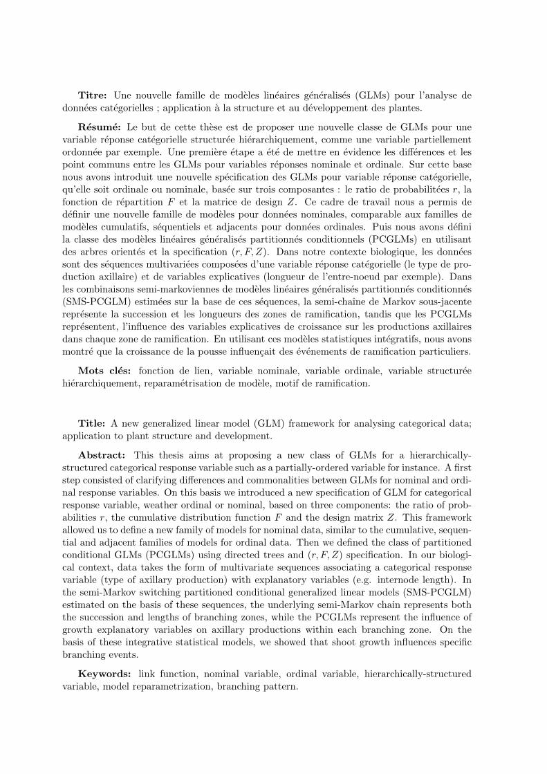
Titre: Une nouvelle famille de modeles lineaires generalises (GLMs) pour l’analyse dedonnees categorielles ; application a la structure et au developpement des plantes.
Resume: Le but de cette these est de proposer une nouvelle classe de GLMs pour unevariable reponse categorielle structuree hierarchiquement, comme une variable partiellementordonnee par exemple. Une premiere etape a ete de mettre en evidence les differences et lespoint communs entre les GLMs pour variables reponses nominale et ordinale. Sur cette basenous avons introduit une nouvelle specification des GLMs pour variable reponse categorielle,qu’elle soit ordinale ou nominale, basee sur trois composantes : le ratio de probabilitees r, lafonction de repartition F et la matrice de design Z. Ce cadre de travail nous a permis dedefinir une nouvelle famille de modeles pour donnees nominales, comparable aux familles demodeles cumulatifs, sequentiels et adjacents pour donnees ordinales. Puis nous avons definila classe des modeles lineaires generalises partitionnes conditionnels (PCGLMs) en utilisantdes arbres orientes et la specification (r, F, Z). Dans notre contexte biologique, les donneessont des sequences multivariees composees d’une variable reponse categorielle (le type de pro-duction axillaire) et de variables explicatives (longueur de l’entre-noeud par exemple). Dansles combinaisons semi-markoviennes de modeles lineaires generalises partitionnes conditionnes(SMS-PCGLM) estimees sur la base de ces sequences, la semi-chaıne de Markov sous-jacenterepresente la succession et les longueurs des zones de ramification, tandis que les PCGLMsrepresentent, l’influence des variables explicatives de croissance sur les productions axillairesdans chaque zone de ramification. En utilisant ces modeles statistiques integratifs, nous avonsmontre que la croissance de la pousse influencait des evenements de ramification particuliers.
Mots cles: fonction de lien, variable nominale, variable ordinale, variable structureehierarchiquement, reparametrisation de modele, motif de ramification.
Title: A new generalized linear model (GLM) framework for analysing categorical data;application to plant structure and development.
Abstract: This thesis aims at proposing a new class of GLMs for a hierarchically-structured categorical response variable such as a partially-ordered variable for instance. A firststep consisted of clarifying differences and commonalities between GLMs for nominal and ordi-nal response variables. On this basis we introduced a new specification of GLM for categoricalresponse variable, weather ordinal or nominal, based on three components: the ratio of prob-abilities r, the cumulative distribution function F and the design matrix Z. This frameworkallowed us to define a new family of models for nominal data, similar to the cumulative, sequen-tial and adjacent families of models for ordinal data. Then we defined the class of partitionedconditional GLMs (PCGLMs) using directed trees and (r, F, Z) specification. In our biologi-cal context, data takes the form of multivariate sequences associating a categorical responsevariable (type of axillary production) with explanatory variables (e.g. internode length). Inthe semi-Markov switching partitioned conditional generalized linear models (SMS-PCGLM)estimated on the basis of these sequences, the underlying semi-Markov chain represents boththe succession and lengths of branching zones, while the PCGLMs represent the influence ofgrowth explanatory variables on axillary productions within each branching zone. On thebasis of these integrative statistical models, we showed that shoot growth influences specificbranching events.
Keywords: link function, nominal variable, ordinal variable, hierarchically-structuredvariable, model reparametrization, branching pattern.