Yue Zhou-Kangas

MODELING AND ANALYSING THE PERFORMANCE OF A WIRELSS MESH NETWORK

UNIVERSITY OF JYVÄSKYLÄ

DEPARTMENT OF MATHEMATICAL INFORMATION TECHNOLOGY

2014

i

ABSTRACT

Zhou-Kangas, Yue Modeling of a wireless mesh network Jyväskylä: University of Jyväskylä, 2014, 60 p. Mathematical Information Technology, Master’s Thesis Supervisors: Professor Hämäläinen, Timo Dr. Petrov, Dmitry

As an emerging technology for the future internet, the wireless mesh networks can provide fast-configure low-cost and scalable wireless networks to large are-as. The wireless community networks are based on the wireless mesh network technology as a new solution for internet access, game, internet radio and VoIP services for the users. This thesis presents the wireless mesh network technology in details including the related routing protocols and standards. The topology data (in CNML) of Guifi.net, an open access community network deployed in Spain, was also ana-lyzed. Based on the topology information parsed from the CNML file, a small zone of Guifi.net was modeled. The performance of the modeled zone was studied via the simulations with the 802.11s mesh module in NS-3. By analyzing the simulation results, the network efficiency and the instantanei-ty of the modeled zone were shown as decreasing with the increasing of the network load. The simulation results also indicated that the efficiency of the links in the modeled zone was not dependent on the hop count distance. From the analysis of the simulation results for peer links, the key factors that affect the performance of the links were identified: the antenna transmission gain of the radio and the distance between the nodes. At the end of the thesis, the idea of the topology generation scheme for Guifi.net is demonstrated. The results from this thesis can provide reference bases for the further steps of the research of the topology generation scheme.

Keywords: Wireless Mesh Network, Wireless Community Network, Topology, Performance, Guifi.net, 802.11s, NS-3.

ii

ACKNOWLEDGEMENTS

First I would like to thank my supervisors Professor Timo Hämäläinen and Dr. Dmitry Petrov for all their support. Dr. Petrov’s brilliant idea of the study on Guifi.net has given the solid base for this study. His guidance and comments repeatedly helped me to carry out the study on this topic. I am grateful for the comments and criticism that Professor Timo Hämäläinen has made for the im-provements of this work.

I extend my thanks to Dr. Margaret Tuomi for reviewing this thesis from

the language and style point of view. Last but not least, I would like to thank my family for their understanding

and assistance.

iii

LIST OF FIGURES

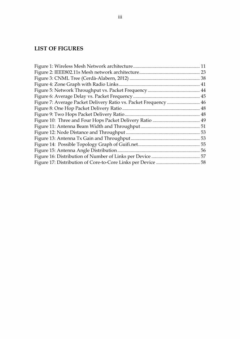
Figure 1: Wireless Mesh Network architecture ....................................................... 11

Figure 2: IEEE802.11s Mesh network architecture .................................................. 23

Figure 3: CNML Tree (Cerdà-Alabern, 2012) .......................................................... 38

Figure 4: Zone Graph with Radio Links ................................................................... 41

Figure 5: Network Throughput vs. Packet Frequency ........................................... 44

Figure 6: Average Delay vs. Packet Frequency ....................................................... 45

Figure 7: Average Packet Delivery Ratio vs. Packet Frequency ........................... 46

Figure 8: One Hop Packet Delivery Ratio ................................................................ 48

Figure 9: Two Hops Packet Delivery Ratio .............................................................. 48

Figure 10: Three and Four Hops Packet Delivery Ratio ....................................... 49

Figure 11: Antenna Beam Width and Throughput ................................................. 51

Figure 12: Node Distance and Throughput ............................................................. 53

Figure 13: Antenna Tx Gain and Throughput ......................................................... 53

Figure 14: Possible Topology Graph of Guifi.net ................................................... 55

Figure 15: Antenna Angle Distribution .................................................................... 56

Figure 16: Distribution of Number of Links per Device ........................................ 57

Figure 17: Distribution of Core-to-Core Links per Device .................................... 58

iv

LIST OF TABLES

Table 1: CNML Elements and Attributes (Cerdà-Alabern, 2012) ......................... 38

Table 2: Parsed Information of the Selected Zone from CNML ........................... 40

Table 3: Distance, Radio Parameters and Throughput .......................................... 50

Table 4: Rearranged Peer Link Throughput ............................................................ 54

v

LIST OF ABBREVIATIONS

ALM Air Link Metric AODV Ad-hoc On-Demand Vector BSS Basic Service Set CNML Community Network Markup Language DO Destination Only DS Distributed System DSDV Destination-Sequence Distance Vector DSN Destination Sequence Number DSR Dynamic Source Routing ESS Extended Service Set ETX Expected Transmission Count FSR Fisheye State Routing HWMP Hybrid Wireless Mesh Protocol IBSS Independent Basic Service Set IETF Internet Engineering Task Force IP Internet Protocol LAN Local Area Network LQ Link Quality MAC Medium Access Control MANET Mobile Ad hoc Network MAP Mesh Access Point MBSS Mesh Basic Service Set MP Mesh Point MPP Mesh Portal MPR Multi Point Relay NS-3 Network Simulator 3 OLSR Optimized Link State Routing Protocol PAN Personal Area Network PREQ Path Request PREP Path Reply PERR Path Error QoS Quality of Service RANN Root Announcement RF Reply-and-Forward RREQ Route Request RREP Route Reply RERR Route Error SFHT Scale Free by Hidden Terminal STA Station

vi

TC Topology Control TTL Time-To-Live VoIP Voice over Internet Protocol WCN Wireless Community Network WMN Wireless Mesh Network WRP Wireless Routing Protocol

vii

LIST OF ATTACHEMENTS

Attachment 1: Python Script for Parsing the CNML File Used in Studying the Small Zone .................................................................................................................... 69

Attachment 2: Simulation Script for Packets Sending from Random Source Node to the Root Node at Data Rate 4096kbps (at Frequency 1 packet /s) ....... 73

viii

TABLE OF CONTENT

ABSTRACT ...................................................................................................................... I

ACKNOWLEDGEMENTS ........................................................................................... II

LIST OF FIGURES ........................................................................................................ III

LIST OF TABLES ......................................................................................................... IV

LIST OF ABBREVIATIONS .......................................................................................... V

LIST OF ATTACHEMENTS ...................................................................................... VII

TABLE OF CONTENT .............................................................................................. VIII

1 INTRODUCTION ................................................................................................. 1

1.1 The Wireless Mesh Networks and The Community Networks ............ 1

1.2 Guifi.net ......................................................................................................... 2

1.3 Means to Study the Modern Wireless Networks .................................... 3

1.4 The Research Framework ........................................................................... 5

1.4.1 Aims of the Thesis and the Research Questions ............................ 5

1.4.2 The Constructive Research Approach ............................................. 6

1.4.3 The Constructive Research Approach Applied in This Thesis .... 7

2 THE WIRELESS MESH NETWORKS .............................................................. 10

2.1 The Wireless Mesh Networks .................................................................. 10

2.2 The Wireless Mesh Network Topology .................................................. 13

3 THE WIRELESS MESH NETWORKS RELATED ROUTING PROTOCOLS15

3.1 The Table Driven Routing Protocols ....................................................... 15

3.1.1 The Fisheye State Routing Protocol (FSR) and the Wireless Routing Protocol (WRP) .................................................................. 16

3.1.2 The Destination-Sequence Distance Vector Routing Protocol (DSDV) ............................................................................................... 16

3.1.3 The Optimized Link State Routing Protocol (OLSR) .................. 17

3.2 The Source Routing Protocols .................................................................. 18

3.2.1 The Ad-Hoc On-Demand Vector Routing Protocol (AODV) .... 18

3.2.2 The Dynamic Source Routing Protocol (DSR) ............................. 19

4 THE WIRELESS MESH NETWORK RELATED STANDARDS ................... 21

4.1 The IEEE 802.15.5 Bluetooth and The IEEE 802.15.4 Zigbee ............... 21

4.2 The IEEE 802.11s Wi-Fi Mesh ................................................................... 22

4.2.1 The Network Structure .................................................................... 23

4.2.2 The Peering Management Protocol ............................................... 24

ix

4.2.3 The Airtime Link Metric .................................................................. 24

4.2.4 The Hybrid Wireless Mesh Protocol ............................................. 25

4.2.5 The MAC Frame and Other Functionalities ................................. 26

5 THE RELATED RESEARCHES ......................................................................... 29

5.1 The Performance Studies on Wireless Mesh Networks ....................... 29

5.2 The Researches of Guifi.net ...................................................................... 32

6 THE NS-3 SIMULATOR AND 802.11S MODULES ....................................... 34

6.1 The Network Simulator 3 ......................................................................... 34

6.2 The 802.11s Mesh Network Implementation in NS-3 ........................... 35

7 THE STUDY ON GUIFI.NET ............................................................................ 37

7.1 The Topology Data of Guifi.net ............................................................... 37

7.2 The Modeling of the Small Zone of Guifi.net ........................................ 39

7.2.1 Use of the CNML Data .................................................................... 39

7.2.2 The Simulation Scenario .................................................................. 42

7.2.3 The Simulation Results .................................................................... 43

7.3 Other Analysis of the Topology Data ..................................................... 54

8 CONCLUSION .................................................................................................... 59

REFERENCES ................................................................................................................ 62

ATTACHMENT S ......................................................................................................... 69

1

1 INTRODUCTION

Nowadays, internet is involved in individuals' life significantly. People use both portable and non-portable devices such as smartphones, laptops, pads, desk-tops and digital TVs etc. to access different applications on the internet. Users are not only with needs such as emails, web-browsing but also other things such as gaming, video-browsing and so on. To meet the rapid growth of users' needs, service providers are trying to offer multiple-featured high speed ser-vices. Traditional networking technology cannot satisfy the demands of these services because of the limitation from bandwidth and construction costs. High speed Internet access can be obtained via the cable broadband such as DSL and Wi-Fi. However, service providers may not deploy such kind of networks in scarcely populated area because of low profitability. Conversely, people who live in such areas also share the equal rights to have high speed internet ser-vices. In addition, there are some situations that the networking cannot be di-rectly or fully supported by traditional wireless technologies. Therefore, Wire-less Mesh Networks (WMNs) become ideal candidates in developing cost-effective high-bandwidth broadband networks.

1.1 The Wireless Mesh Networks and The Community Networks

The WMNs provide flexible, fast-configure, inexpensive networks via the multi-hop connections among nodes. The nodes can freely join and leave such networks (Akyildiz and Wang, 2005). They can be used for a wide range of ap-plications such as broadband internet access, online gaming, video streams etc. They can also serve in various locations such as conferences, hotels, airports, neighborhoods and so on (Natkaniec, 2009). In addition, the WMNs can play an important role in disasters when the communication infrastructure is damaged. They also receive notable attentions from military forces.

2

Wireless Community Networks (WCNs) are implemented based on WMN technologies. They are particularly useful in under-developed countries and isolated areas which do not have the traditional network infrastructure. The inexpensive laptops and mobile devices which have abilities to connect to Wi-Fi have driven the initiatives to create WCNs. The WCNs can also provide low-cost and participatory connectivity for citizens for internet access, online infor-mation and application sharing and so on. There are realizations of the WCN world wide such as Guifi.net, Athens Wireless Metropolitan Network, Funk-Feuer, Seattle Wireless and Consume. Establishing a WCN can bring the neigh-borhood many advantages. For example, the internet is shared among neigh-bors in a cost-effective way. Gateways are deployed in a distributed fashion in the neighborhood instead of installing gateways for each individual user. Neighbors also share an online neighborhood network which can include busi-ness information, school information and so on. Furthermore, the remarkable feature of WCNs is that it can be established by the users themselves without involving the service providers and they can grow as needed after initial instal-lation. However, the installation by the users themselves results in the organic growth of the network topology in a decentralized fashion. To maintain the scalability, stability and openness of the WCNs, it is worthy of detailed study on the topology of WCNs. The analysis on the topology information of WCNs can contribute significantly to resolving the main issues faced by the WCNs such as the network performance evaluation, user experiences on the services provided by the network and so on (Vega et al, 2012; Cerdà-Alabern et al. 2012).

1.2 Guifi.net

Guifi.net is a neutral, independent Wi-Fi community mesh network. It is mainly deployed in Catalonia, Spain, with more than 21,807 operational nodes and more than 40,000 km of links still with an exponential growth (Guifi.net).

Guifi.net consists of a set of nodes interconnected through mostly wireless equipment. The equipment are installed and maintained by the users them-selves like individuals, companies, administrations or universities on their building rooftops. The majority of Guifi.net consists of static bidirectional wire-less links setup using Linux powered Wi-Fi devices. In Guifi.net, there is no a-priory overall growth planning instead the growth is driven by users' needs. This kind of growth resulted in a network structure relevant to the geographical distribution. The nodes in Guifi.net, except pure end-user client nodes, act as a Wi-Fi routing device. These nodes provide at least data link and IP forwarding services to connect to all other users and nodes. Proxy nodes act as gateways to provide the internet connectivity, such as the web or VPN proxies, to some members of the community. Most of the links in Guifi.net are point-to-point links between two distant locations using the 2 or 5GHz ISM unlicensed radio

3

bands. Shorter range links use sectorial antennas because sectorial antennas allow one node to reach more nodes rather than only one connected node. This allows running mesh routing protocols like optimized link status routing proto-col to dynamically select which links to use for routing among the available ones. Finally there are many nodes that act as leaf nodes connecting just one end-user with a multipoint access point. Such kind of leaf nodes are referred as terminal nodes Guifi.net while other nodes having more than one link are called core nodes (Cerdà-Alabern, 2012, Vega et al. 2012).

1.3 Means to Study the Modern Wireless Networks

The WMNs have gained much attention as a promising technology (i.e. Efstanthiou, Frangoudis and Polyzos, 2006; Szabó, Horávth and Farkas, 2007; Valle et al, 2008; Calcada, Cortez and Ricardo, 2012). Researches concerning WMNs are done in similar ways as other modern wireless networks.

Modern wireless networks can be studied by mathematical analysis on the

measurements taken from the real network devices. However, this is not realis-tic in development studies and experiments. Common ways to study the wire-less networks in development and experiments are testbeds and computer sim-ulations of the wireless networks.

Testbed is a platform for experimenting. It is built up with real network

devices. Computer simulation is used as a tool to evaluate the performance of a network, existing or proposed, under different configurations and over long periods of time. A Simulation of a wireless network is based on the operation of the model of the network. The measurements are taken from the model opera-tion. The simulation scenario can be reconfigured and experimented with dif-ferent parameters (Maria, 1997). Tan et al. (2011) summarized that the testbed experiments and the computer simulations have both advantages and disad-vantages. The main advantage of testbed experiments is the practicality, be-cause the equipment and software used in the testbed environment can be ac-cessed. The main disadvantage of testbed experiments is the cost, since build-ing a wireless network testbed requires hardware and labor source. In addition, the results of testbed experiments can be heavily influenced by the testing envi-ronment, because the environment criteria like temperature and humidity are usually highly random and uncontrollable. As for computer simulations, the main advantage is the flexibility: the network scenarios can be constructed and modified with relevantly much lower costs, and the results can be achieved in shorter time period. This advantage allows the easier analysis on the networks with different assumptions. The biggest disadvantage of the computer simula-

4

tions is the possible less trustworthy results from the inadequate modeling of the simulated network.

Computer simulations are used to study various issues in wireless net-

works including signal processing in the physical layer, medium access in the link layer, routing at the network layer, protocol issues in the transport layer and design considerations in the application layer. The Computer simulations consist of three main components: a model of the simulated networks, the simu-lation of the network activities and the analysis of the results. Maria (1997) in-troduced an eleven-step simulation process:

Step 1. Identify the problem: Identify the problems in an existing system and produce requirements for a proposed system.

Step 2. Formulate the problem: Define the objectives of the study; the way to evaluate the simulation results; the time frame of the study and form up hypothesis.

Step 3. Collect and process real system data: collect data of the system specifications and design the input parameters for variables.

Step 4. Formulate and develop a model: study the flow of the entities in the system and translate the entities into the form that the simulation software accepts and verify that it executes as designed.

Step 5. Validate the model: compare the measurements under known conditions taken from the simulation with the measurements of the real system.

Step 6. Document the model for future use: document the objectives, as-sumptions and input variables in detail.

Step 7. Select the appropriate experimental design: select the way of re-sult analysis and the variables that are likely to affect them and docu-ment the design.

Step 8. Establish the experimental conditions for runs

Step 9. Perform the simulation runs

Step 10. Interpret and present the results: compute the numerical esti-mates of the desired performance measures for each configuration of the simulation and test the hypothesis.

Step 11. Recommend the further course of action

5

The author also pointed out that the eleven-step is a logical ordering of the

steps in a simulation study, but the actual steps and activities in the study may vary in different cases.

1.4 The Research Framework

1.4.1 Aims of the Thesis and the Research Questions

This thesis aims at achieving three aspects:

1. To gain a deep understanding of the wireless mesh networks including the topologies, the related routing protocols and the standards of the wireless mesh networks especially the IEEE 802.11s standard.

2. To understand the CNML data and familiarize with the Network Simulator 3 (details on CNML can be found in section 7.1 and details on network simulator 3 can be found in section 6)

3. To model a small part of Guifi.net using the CNML data and study the performance of the modeled part with the computer simulations using NS-3.

Based on the goal of the thesis, the following research questions are raised to help to achieve the goals:

1. What are wireless mesh networks?

In order to answer this question, several issues must be addressed: 1) What is the structure of the WMNs?

2) What are the characteristics of the WMNs?

3) What routing protocols are used in the WMNs?

4) What are the existing standards for the WMNs?

5) What does the IEEE 802.11s mesh network standard define?

6) How is the IEEE 802.11s mesh network implemented in NS-3?

2. What are the critical the elements and attributes in CNML data concerning the study of the Guifi.net?

3. How does the modeled zone of Guif.net perform?

6

1.4.2 The Constructive Research Approach

The constructive approach is a research procedure for producing innova-tive constructions to solve real world problems. The innovative constructions contribute to the field of study where it is applied (Piirainen and Gonzalez, 2013). Piirainen and Gonzalez (2013) also pointed out: “Construction” means deliberate design of a thing, as opposed to emergent socially constructed phe-nomena and artifacts. The research result should demonstrate how the problem can be understood, explained, modeled and solved. When solutions to the problems have already been presented, the research result should approve itself as a newer or better solution as well. As to the research itself, it should have practical relevance and practical functioning that are connected to theory and it should be able to contribute to theory (Kasanen, Lukka and Siitonen, 1993). Lindholm(2008) described the constructive method as “ a solution-oriented normative method where target-oriented and innovative step-by-step devel-opment of a solution are combined, and which empirical testing of the solution is done and utility areas are analyzed”. The constructive research approach is chosen for this thesis because of the need for gaining an integrated deep under-standing of the wireless mesh networks in theory and the performance analysis of the practically existing wireless mesh network, Guifi.net. In addition, this thesis is included in the research of the topology generator for Gufi.net to con-tribute further to the wireless mesh network topology in theory. The construc-tive approach is reported to suit well for these purposes (Lukka, 2002).

The constructive research approach originally appeared in the field of management accounting in 1980s and it has been developed in business admin-istration domain (i.e. Kasanen, Lukka and Siitonen, 1993; Singer et al., 2007). It also receives some attention in other fields such as information systems and technical sciences (i.e. Gregor, 2006).

Lindholm (2008) summarized the seven steps of the constructive research ap-proach according to the presentation of Kasanen et al (1993), Lukka (2000), Labro and Tuomela (2003) :

Step 1: Find a practical relevant problem which also has research poten-

tials. Step2: Examine the potential for long-term research co-operation with the

target organization. Step 3: Obtain a general but comprehensive understanding on the research

problem. Step 4: Innovate and construct a theoretically grounded solution idea.

7

Step 5: Implement the solution and test whether it works in practice. Step 6: Examine the scope of the solution’s applicability Step 7: Demonstrate the theoretical connections and the research contribu-

tion of the solution. Lindholm (2008) also pointed out that most steps in the constructive re-

search approach overlap with the previous steps and the following steps. The step of obtaining comprehensive understanding of the research problem con-tinues throughout the whole process.

1.4.3 The Constructive Research Approach Applied in This Thesis

The processes of constructive research approach applied in this thesis are described as follow:

1. Find the research subject.

The research result should produce practical contribution to the

problem. At the same time, the results should have potential for fur-ther research. The wireless mesh network is an emerging technology for future internet. The WCNs is based on wireless mesh network and they are organized and deployed by the cooperation of their own us-ers. The network topology of WCN grows organically without a strict-ly planned deployment or any consideration other than connecting from new participating nodes to the existing ones. Guifi.net is de-ployed in this way. The participants freely collaborate in creating new links by installing and configuring the new hardware devices. The new links expand the network and increases its coverage. The new devices and links are not in guarantee of contributing to or improving the overall capacity of the network but satisfying individual needs.

The network topology impacts on the performance of the net-

work. It is important to gain a clear understanding on the performance of the network that is grown on such model as Guifi.net. The wireless mesh network topology has been explored to details by researchers and WCN also gained some attention. However, researches on the to-pology and the performance relation of WCN were incomplete. The details on the related researches are presented in Section 5.

2. The data used for analysis comes from Guifi.net. Guifi.net provides an

open access to the CNML file and it is periodically updated. In

8

addition, this thesis is guided and supported by a local organization which expertise in wireless technologies. The idea itself comes from the organization. The author of the thesis receives detailed guidance from the organization personnel in addition to the university supervisor.

3. As Lindholm (2008) pointed out, the adequate knowledge of the topic is obtained throughout the whole process. The author studies the literature related to the wireless mesh networks and gains knowledge during the process. The gained knowledge eventually answers the research questions 1 and 2.

4. Based on the detailed knowledge on wireless mesh networks, the author is able to obtain the critical information from the CNML file needed in the performance study of the selected small zone of Guifi.net. The information obtained for the performance study is used as the input parameters in the computer simulations. The computer simulations provide results as the performance metrics, thus the author can analyze the performance of the small zone of Guifi.net.

5. After the analysis, the author can present the evaluation and identify the key factors that are affecting the performance of the small zone of Guifi.net. In this thesis, it is clear that the performance evaluation and the key factors that are affecting the performance of the network are only valid for the selected small zone within the scope of the thesis. In addition, the idea of topology generator for Guifi.net is presented.

6. Further validation of the performance evaluation and key factors that are affecting the network performance are needed. This need points out the potential for further researches on the results. The further researches can be done by studies for more small zones as well as bigger zones. The development on the topology generator will continue as the future work right after the performance study and eventually become a validated topology generator for WCN like Guifi.net.

7. As stated before, studying the topology of Guifi.net can contribute to resolving the issues faced by WCNs such as Guifi.net. Within the scope of this thesis, the author can understand the performance of the selected zone and identify the key factors affecting the network performance. This can already indicate the situation other zones with similar characteristics, and suggest to the network users on the aspects that they need to consider. With the further studies after this thesis, suggestions can be made in more general level.

The reminder of the thesis is organized as follow: Chapter 2, 3 and 4 pre-

sent the detailed study on the wireless mesh networks from literature including

9

the detailed general description, the topology of wireless mesh networks, and the wireless mesh network related routing protocols and the wireless mesh network standards. Chapter 5 presents the related research. Chapter 6 introduc-es the Network Simulator 3, the simulation tool used in this thesis study. Chap-ter 7 describes the study of Guifi.net including the CNML data of Guif.net and Guifi.net itself, the analysis of CNML data, the modeling of a small zone of Guifi.net and the idea of the topology generator for Guifi.net. And finally, Chapter 8 concludes this thesis and presents the possible directions of future work.

10

2 THE WIRELESS MESH NETWORKS

This section includes more detailed description on the wireless mesh networks, the different categories of wireless mesh networks, the characteristics of wire-less mesh networks and the wireless mesh networks topology.

2.1 The Wireless Mesh Networks

WMNs are dynamically self-organized and self-configured. The architecture is composed of two types of mesh nodes: mesh routers and mesh clients (Akyildiz and Wang, 2005). Mesh routers have routing functions for supporting mesh network in addition to same functions of the conventional routers. They are also used as network coverage extenders. One of the main functions of mesh routers is to relay data to other mesh routers. Some mesh routers serve as gateways with a link to the backbone network. Some mesh routers are also used as access points (APs) to provide connections to mesh clients. Mesh clients connect to the WMN via APs with either wireless or wired links with a wide variety of devices like smartphones, PDAs, laptops and desktops and so on (Afanasyev et al. 2010).

The meshing among the mesh routers creates a wireless backhaul communication system. The network provides clients a low-cost, high-bandwidth and seamless multihop interconnection service (Yu, Xu and Wu, 2010). The traffic originated in the client devices traverses the wireless backhaul. The mesh routers relay the data with wireless radio links and the mesh routers with gateway function connect to the backbone network. The backbone network can be almost any type of network such as LAN, DSL or 3G/4G networks. Figure 1 adapted from literature illustrates the mesh network architecture (Bruno, Conti and Gregori, 2005).

11

Figure 1: Wireless Mesh Network Architecture

According to Rabbi (2006), there are three types of Mesh networks:

Client WMNs: they are similar to mobile ad-hoc networks (MANETs). They provide peer-to-peer communication among client devices. Mesh routers are not needed in client WMNs. Mesh clients form up the actual network and perform routing and configuration functions in addition to providing applications to end-users. What makes client WMNs different from MANETs is the mobility of mesh nodes. In client WMNs, the mesh nodes have low mobility while in MANETs the mesh nodes are mobile. One laptop per child project (one laptop per child) is an example of client WMN.

Infrastructure/backbone WMNs: the mesh routers with gateway functionality are connected to the backbone networks for example the internet. Other mesh routers which do not have the gateway functionality send data to and receive data from the backbone network via the connection to the gateway nodes. The mesh routers relay and route traffic from mesh nodes toward the final destination. The final destination can be within the mesh or to other networks which the

Backbone Network

Figure 1: Wireless Mesh Network architecture

Mesh Gateways

Mesh Routers

Mesh Client

Gateway Connection

Wireless Connection

12

gateway nodes are connected to. The MIT RoofNet (RoofNet-Introduction) is an example of infrastructure WMN.

Hybrid WMNs: they are combination of infrastructure and client WMNs. In hybrid WMN, the mesh clients are also interconnected as well as the mesh routers. The transportation of data can be from users to other users or the mesh routers. Both infrastructure WMNs and hybrid WMNs are adaptable to other networks such as the internet, WiMAX, cellular networks and sensor networks.

The key characteristics of the WMNs can be studied from the aspects of the

mesh topology creation, routing, security, quality of service and power efficiency (Faccin et al. 2006). Akyildiz and Wang (2005) outlined the characteristics of hybrid WMNs:

The WMNs are multi-hop wireless networks: the aim is to achieve higher throughput at the same time as guaranteeing the network coverage, lower interference between nodes and the efficient frequency re-use.

The network architecture of WMNs is flexible: WMNs support ad-hoc networking, and they are capable of self-forming, self-healing and self-organization. The deployment and configuration are relevantly easy with low initial costs. The network can grow gradually according to needs.

Different types of mesh nodes have different levels of mobility: Mesh routers have minimal mobility while mesh clients can be either stationary or mobile.

The WMNs support multiple types of network access: the WMNs provide access to the backbone network which the gateway nodes are connected to. They also support peer to peer communication.

Different types of mesh nodes have different dependency on power-consumption constraints: the low mobility mesh routers usually do not have strict constraints on power consumption. The mesh clients and some stand-alone mesh nodes like the repeaters in distant area need power efficient protocols.

The WMNs are capable of inter-operating with different wireless networks like IEEE 802.11 networks, WiMAX networks and cellular networks.

The characteristics also distinguish the WMNs from MANETs. The mesh routers perform dedicated routing and configuration functions, which significantly decreases the load of mesh clients and other end nodes. Mobility of the end nodes is supported easily through the wireless infrastructure. Mesh routers are integrated to heterogeneous networks, both wired and wireless.

13

Thus, multiple types of network access exist in WMNs. Power consumption constraints are different for different kinds of mesh routers depending on the location and the mobility of the nodes. A WMN is not stand-alone and it should be compatible and interoperable with other wireless networks.

2.2 The Wireless Mesh Network Topology

Held (2005) described the term “node” as a communication device that can transport data from one of its interfaces to another device. The author also considered the ability of each node to communicate with other nodes in the network as the representation of a mesh network topology.

The nodes in the WMNs automatically establish and maintain the mesh connectivity among them. They operate as routers in addition to hosting and forwarding packets on behalf of other nodes that may not be within direct wireless transmission range of the destinations (Akildiz and Wang, 2010). When a new node is added to the network, it can automatically configure itself and determine the best multi-hop transmission paths. When there are changes of the nodes, the network can discover the topology change automatically and adjust accordingly (Yu, Xu and Wu. 2010).

The formation of the WMN topology is influenced by many factors like link quality, the mobility of the nodes, the availability of the nodes and network deployment and so on. These factors influence the design and performance of the routing protocol(s) used in the network. Akildiz and Wang (2010) suggested that the distributed topology discovery scheme is a better choice for WMNs, because of the distributed nature of the WMNs. The topology discovery process provides the network topology and other related information to the routing protocol. The purpose of the topology discovery process is to obtain the up-to-date topology information. An efficient information exchange scheme is needed to distribute and collect topology information. The improvement of the efficien-cy of the topology information exchange can be achieved from the considera-tion of the frequency of information exchange, the contents of the signaling messages and so on.

The creation of mesh network topology is a three phase process including

the discovery phase, the associating and forming phase and the updating phase. When a node is activated, it starts to discover mesh networks that are present for associating. If no network is detected, the node initiates a new one. There are two approaches of network discovery: a passive approach (also referred as on-demand or reactive approach) and an active approach. The passive approach means that when a node receives the beacon messages from other nodes, it discovers the existing mesh networks. The active approach means that

14

the nodes send probing messages in order to discover existing mesh networks. After discovering the basic connectivity in the network, the nodes will associate with the one hop neighbor nodes. After identifying and associating with all the nodes, the connected group of nodes with too large size may be divided into smaller mesh networks operating on different channels. The smaller clusters of wireless mesh networks are interconnected by the gateway nodes. Same beacon messages used for network discovery are transmitted periodically for the topology maintenance. They carry the information of the current state of the network to the nodes, so that the nodes can refresh their connectivity association and update if necessary (Faccin et al. 2006). Liu and Bai (2012) pointed out that recently WMN has involved operating on multi-radio multi-channel architecture to overcome high latency and improve the throughput. Details of the routing protocols used in WMNs are discussed in Section 3.

15

3 THE WIRELESS MESH NETWORKS RELATED ROUTING PROTOCOLS

A routing protocol is to find an efficient outing path to send data packets from the source node to the destination node. The major goals for a routing protocol are: selecting alternative reliable routes fast and efficiently if the node connec-tivity fails; selecting an efficient path with least cost and providing the best re-sponse time, short delay and high throughput.

A MANET is a network without a fixed infrastructure, in which the nodes

belonging to a MANET can either be end-points of a data interchange or can act as routers when the source and destination nodes are not directly within their radio range. Ad hoc routing protocols must operate in a distributed fashion al-lowing each node to enter and leave the network on its own. The routing proto-cols should avoid data looping in the network. The nodes operate in either the proactive or reactive mode. Similar to the wired networks, the proactive proto-cols are table-driven and usually the routes to other nodes in the entire network are maintained within each node. The nodes must be in continuous communi-cation about the changes of the network topology. This type of routing proto-cols is suitable for real-time applications and the QoS guarantees due to the low-latency. For very dynamic topologies, the proactive protocols can introduce large overheads in bandwidth and energy consumption in the network. The reactive protocols trade off the overheads with the increased delay. A route to a destination is established when it is needed based on an initial discovery be-tween the source and the destination nodes (CIER Deliverable).

3.1 The Table Driven Routing Protocols

Table-driven (proactive) routing protocols attempt to maintain the con-sistent, up-to-date routing information from each node to every other node in the network. These protocols require each node to maintain one or more rout-

16

ing tables to store the routing information. A consistent network view is main-tained in response of the network topology change by propagating the updates throughout the network. The routing information is exchanged in the back-ground regardless of the communication requests. The difference among differ-ent proactive routing protocols is the number of necessary routing-related ta-bles the nodes have to maintain and the broadcasting methods by which the changes in network structure are broadcasted. The Destination-Sequenced Dis-tance-Vector (DSDV) routing protocol, the Fisheye State Routing (FSR) protocol, the Optimized Linked State Routing protocol (OLSR) and Wireless Routing Pro-tocol (WRP) are examples of table driven routing protocols. This section dis-cusses FSR and WRP in brief followed by a more detailed description of DSDV and OLSR.

3.1.1 The Fisheye State Routing Protocol (FSR) and the Wireless Routing Pro-tocol (WRP)

FSR is based on link state routing algorithm. The link state status is ex-changed periodically in FSR, and each node keeps a full topology map of the network. The key improvement in FSR is that different update periods are used for different entries in the routing table so that the overheads caused by main-taining the network topology information are effectively reduced. For the nodes within a smaller scope, the link state updates are propagated in a higher fre-quency. The accurate distance and path quality of the route to the immediate neighboring nodes is maintained. Such information is progressively reduced in details with the increases of the distance (Gerla, Chen and Pei, 2002).

In WRP, each node maintains three tables and a list: the distance table, the

routing table, the link-cost table and the message retransmission list. Based on the tables and list, route information can be obtained for example the cost of the link connecting to the neighbor and the number of timeouts when an error-free message was received from that neighbor. A node validates its neighbors after detecting any link change to eliminate the loops and speed up convergence. Based on the above mentioned feature of WRP, it is ensured that the update messages are exchanged reliably and route loops are reduced (Kumar and Ku-mar, 2012).

3.1.2 The Destination-Sequence Distance Vector Routing Protocol (DSDV)

The DSDV routing protocol is one of the first protocols proposed for wire-less Ad Hoc Networks. Each node maintains a table that contains information of a set of the current neighbors: the minimum distance and the first node on the shortest path to every destination node in the network. Messages directed to the destination are routed through the next hop neighbor along the route (Boukerche, 2004). The increasing sequence number tags are used in the up-

17

dates of the routing tables in order to prevent loops, to deal with count-to-infinity problem, and for faster convergence. The routes to all the destinations are available at every node at all the time. The route update is done by periodi-cally broadcasting but it can also be triggered by any changes of the network topology. The nodes in the network are required to periodically advertise their routing tables to their neighbors. The routing tables are exchanged at regular intervals of time so that an up-to-date view of the network topology is main-tained. The tables are also forwarded if a node observes a significant change in local topology. The table updates can either be incremental or full dumps. In-cremental updates are done when the node does not observe significant chang-es in the local topology. The table updates are initiated by the destinations with a new sequence number which is always greater than the previous one. Upon receiving the table, a node may either update its routing table or wait for anoth-er table from its next neighbor. Based on the sequence number of the table up-date, the node may forward or reject the table. One of the drawbacks of this routing protocol is that updates due to broken links lead to high control over-head with high nodes mobility. Another drawback is the stale routes: in order to obtain information about a particular destination node, a node has to wait for a table update message initiated by the specific destination node (CIER deliver-able).

3.1.3 The Optimized Link State Routing Protocol (OLSR)

The OLSR routing protocol is an optimization over the classical link state protocol, tailored for mobile ad hoc networks. Three mechanisms are used in routing. First, periodic “HELLO” messages are used for neighbor sensing. The nodes use “HELLO” messages to find its one-hop neighbors (if and only if it can be reached via bi-directional link) and its two-hop neighbors by the re-sponses of the neighbors. After the neighbor lists are filled, topology infor-mation is exchanged by means of Topology Control (TC) packets. Second, Only Multi Point Relays (MPRs), which are selected nodes, are used to retransmit TC messages in order to minimize the overhead of flooding of the control traffic. MPRs provide an efficient mechanism for flooding control traffic by reducing the number of transmissions required. Third, optimal path is selected using shortest path first mechanism (Gupta and Gupta, 2013).

OLSR is one of the most popular link state routing protocols in the open

source world. It performs on IP layer and is optimized for mobile and wireless ad-hoc networks. OLSR is a proactive routing protocol, which builds up a route for data transmission by maintaining a routing table inside every node in the network. The routing table is computed upon the knowledge of the topology information. The sender node selects its MPR based on the one-hop neighbor nodes, which offer the best routes to the two hop nodes. Each node has also an MPR selector set which enumerates the nodes that have selected it as the MPR node. OLSR uses TC messages along with MPR forwarding to disseminate

18

neighbor information throughout the network. OLSR checks the symmetry of neighbor nodes by means of a 4-way handshake based on the “HELLO” mes-sages. The handshake is inherently used to compute the packet loss probability over a certain link. It is necessary to mention that the original definition of OLSR does not include any provisions for sensing the link quality. It simply assumes that a link is up if a number of “HELLO” packets have been received recently. The implementations such as the open source OLSR (commonly used on Linux-based mesh routers) have been extended with link quality sensing. The Link Quality (LQ) extensions to OLSR introduce the new kind of “HELLO” messages, which are called “LQ HELLO” messages. For each link listed in such a message, the originator of the messages also tells the link quality. So, each neighbor puts the LQ values that it has determined in the message. This gives necessary information to calculate the Expected Transmission Count (ETX) for each link between a node and one of its neighbors (CIER Deliverable).

3.2 The Source Routing Protocols

A different approach from table-driven routing is source-initiated on-demand (reactive) routing. This type of routing creates routes only when they are desired by the source node. When a node requires a route to a destination, it initiates a route discovery process within the network. This process is complet-ed once a route is found or all possible route permutations have been examined. When a route has been established, it is maintained by a route maintenance procedure until either the destination becomes inaccessible or until the route is no longer desired. The Ad-Hoc On-Demand vector Routing (AODV) protocol, the Dynamic Source Routing (DSR) protocol, the Temporally Ordered Routing Algorithm (TORA) routing protocol and the Associativity-Based Routing (ABR) protocol are examples of on-demand routing protocols. In this section, AODV and DSR are discussed.

3.2.1 The Ad-Hoc On-Demand Vector Routing Protocol (AODV)

The AODV routing protocol is an on-demand reactive protocol that uses the distance vector routing algorithm. It only maintains the routing information of the active paths. The routing information is maintained in next-hop routing tables at nodes. The next-hop routing table contains the current known routes to destinations of a node. The routing table entry expires if it has not been used or reactivated for the pre-specified expiration time. The ADOV routing protocol adopts the destination sequence number technique used by DSDV in an on-demand way (IETF, 2003). The AODV routing protocol has also been designed to reduce the dissemination of control traffic and to eliminate overhead on data

19

traffic to improve scalability and performance. This protocol uses the messages RREQ (Route Request), RREP (Route Replies) and RERR (Route Errors). In the AODV routing protocol, nodes discover routes in the request-response cycles. The major difference between the AODV routing protocol and other on-demand routing protocols is that it uses the Destination Sequence Number (DSN) to determine an up-to-date path to the destination. A node updates its path information only if the DSN of the current received packet is greater than the last DSN stored at the node. When an intermediate node receives a RREQ, it either forwards it or prepares a RREP if it has a valid route to the destination. All nodes that are active in the network transmit periodically “HELLO” mes-sages (considered as special RREP messages). If one node does not receive a “HELLO” from the neighbors it means that the connection has been lost and the node modifies the routing table by deleting that path. The node also sends a RRER to other neighbor nodes that used that path.

One of the disadvantages of this protocol is that intermediate nodes can

lead to in-consistent routes if the source sequence number is very old and if the intermediate nodes have a higher but not the latest destination sequence num-ber, thereby having the stale entries. Also multiple RREP packets in response to a single RREQ packet can lead to heavy control overheads. Another disad-vantage of AODV is that the periodic beaconing leads to unnecessary band-width consumption (CIER Deliverables).

3.2.2 The Dynamic Source Routing Protocol (DSR)

The DSR routing protocol is a reactive routing protocol, which uses source routing to deliver data packets. The network is completely self-organized and self-configured requiring no existing network infrastructure or administration. The route discovery mechanism and the route maintenance mechanism work together in DSR. The route discovery mechanism is used only when a node at-tempts to send a packet to a destination without a known route. The route maintenance mechanism is used when a route is discovered and the actual packets transmissions are in process. When the network topology is changed, the route maintenance mechanism may indicate broken source routes. Then the node can attempt to send packets by other route it happens to know or start new route discovery (Kumar and Kumar, 2012).

Headers of data packets carry the sequence of nodes through which the

packet must pass by. This means that intermediate nodes only need to keep track of their immediate neighbors in order to forward data packets. The source, on the other hand, needs to know the complete hop sequence to the des-tination. As in AODV, the route acquisition procedure in DSR requests a route by flooding a RREQ packet. A node receiving the RREQ packet searches its route cache, where all its known routes are stored, for a route to the requested destination. If no route is found, it forwards the RREQ packet further on after

20

having added its own address to the hop sequence stored in the RREQ packet. The Route Request packet is propagated through the network until it reaches either the destination or a node with a route to the destination. If a route is found, a RREP packet containing the proper hop sequence for reaching the des-tination is unicasted back to the source node. DSR does not rely on bi-directional links since the RREP packet is sent to the source node either accord-ing to a route already stored in the route cache of the replying node, or by being piggybacked on a RREQ packet for the source node.

The DSR protocol has the advantage of being able to learn routes from the

source routes in the received packets. To avoid unnecessarily flooding the net-work with RREQ messages, the route acquisition procedure first queries the neighboring nodes to see if a route is available in the immediate neighborhood. This is done by sending a first RREQ message with the hop limit set to zero, thus it will not be forwarded by the neighbors. If no response is obtained by this initial request, a new RREQ message is flooded over the entire network.

The disadvantage of this protocol is that the route maintenance mecha-

nism does not locally repair a broken link. Stale route cache information could also result in inconsistencies during the route reconstruction phase. The connec-tion setup delay is higher than in table-driven routing protocols. Even though the protocol performs well in static and low-mobility environments, the per-formance degrades rapidly with increased mobility. Also, considerable routing overhead is involved due to the source-routing mechanism employed in DSR. This routing overhead is directly proportional to the path length (CIER Deliver-able).

The routing protocol in wireless mesh networks is a popular topic in re-

search field. There are some proposed routing protocols which involve some optimization goals, such as energy efficiency (i.e. Yang and Ma, 2007) and net-work resource management (i.e. Shah, Fransesco and Kumar, 2013). Most of the proposed routing protocols are based on some of the traditional ad-hoc network routing protocols introduced above.

21

4 THE WIRELESS MESH NETWORK RELATED STANDARDS

In addition to attracting attentions from academia, the WMNs also received attentions from the industry. There are researches on the WMNs related equipment and technologies carried out by many companies such as Cisco Sytems, Motorola, Nortel Networks and so on. IEEE has also developed different mesh network related standards. Some of the mesh network related IEEE standards are summarized in this section.

The IEEE 802 family of standards is dedicated to the construction of Local Area Networks (LANs) and Metropolitan Area Networks (MANs). IEEE 802.11 Standard specifies the physical, MAC and link layer operations for wireless LANs (Heirtz, 2010).

4.1 The IEEE 802.15.5 Bluetooth and The IEEE 802.15.4 Zigbee

15th working group of IEEE 802 organized a task group, group 5, to deal with issues related to Wireless Personal Area Networks (PANs). This group determined the necessary mechanisms that must be provided in the physical and MAC layer to enable mesh networking in Wireless PANs. Bluetooth is the commercial name for the developed standard. This standard introduced two possible mesh topologies for Wireless PANs: full mesh topology and partial mesh topology. In full mesh topology, all the mesh nodes are fully intercon-nected. In partial mesh topology, some nodes are connected to all the other nodes while some are only connected to the data relaying nodes (IEEE 802.15.5 Bluetooth).

22

Originally proposed by Motorola, IEEE 802.15.4 Zigbee supports mesh to-pology in Wireless PANs in multi-hop fashion by defining a coordinator which is responsible for configuring the network topology (IEEE 802.15.4 Zigbee).

4.2 The IEEE 802.11s Wi-Fi Mesh

The Wireless Mesh Networks provide reduced infrastructure costs for ac-cess networks spanning up to hundreds of square kilometers by reducing the use of costly wired entry points that supply access to the Internet (Bruno, Conti and Gregori, 2005). City-wide two-tier (backhaul tier –mesh node to mesh node and an access tier –mesh node to client) mesh networks are becoming more and more attractive for metropolitan areas. Many cities have already deployed mesh networks to assist public services and safety personnel such as the New Orleans in USA, the FunkFeuer network in Austria and the San Mateo in Spain and so on. Moreover in the Internet Engineering Task Force (IETF), the MANET work group has standardized many multihop routing protocols such as the Ad Hoc On-Demand Distant Vector (AODV) routing protocol, the Dynamic Source Routing (DSR) protocol, and the Optimized Link State Routing (OLSR) protocol and so on (see section 3 for details on these routing protocols).

In September 2003, IEEE started a study group to investigate adding wire-less mesh network as an amendment for its IEEE 802.11 standards. One year later, the study group became the task group “S”, which issued the first draft later in March 2006. This amendment describes protocols for IEEE 802.11 sta-tions to form self-configured multi-hop networks that support both broad-cast/multicast and unicast data delivery. The amendment defines the mesh network structure, the node category, the mesh network creation and manage-ment mechanism, the characteristics of a 802.11s mesh network, the path selec-tion mechanism and the coordination function for MAC in different categories of mesh node. The amendment also addresses the security and congestion con-trol issues (IEEE Standard for Information Technology, 2011).

The first multihop wireless networks used layer three (IP) mechanisms to relay packets from the source to the destination. Since wireless links are less reliable than wired links, a multihop routing protocol operating in wireless en-vironment must account for the nature of the wireless links. Thus IETF’s MA-NET protocols are forced to rely on indirect measurements to observe the radio environment. However, the MAC layer has adequate knowledge of its meas-urements less outdated and more precise. To realize the benefits a MAC-based WMN promises, an integrated mesh networking solution was developed in IEEE 802.11 Task Group S (Carrano et al. 2007). Since MAC-based multihop so-lutions inherently support layer 2 traffic, they operate transparently to any higher-layer protocol. Each mesh station participation in the 802.11s wireless mesh network operates as link layer router.

23

To provide efficiently bandwidth over large coverage areas, IEEE 802.11s standard deals with the following main challenges (Camp and Knightly, 2008):

The efficient use of limited resources (capacity and time) since in-termediate mesh nodes are used both to source and forward data over the mesh.

The protection and conservation of resources: securing data and conserving power for long-term operation of mobile wireless devic-es.

Providing fairness via mesh congestion control: nodes closer to gateway should not achieve higher throughput than mesh nodes of greater hop count.

4.2.1 The Network Structure

The most elementary 802.11 network is called the Basic Service Set (BSS). The BSSs can form up Extended Service Set (ESS). The BSS can consist, for ex-ample, of wireless Access Point (AP) and stations (STAs) associated with it. Distribution System (DS) provides the services that are necessary to communi-cate with devices outside of its own BSS, so the individual clients can have ac-cess to the internet. Independent Basic Service Set (IBSS) has only one BSS with-out an integrated wired LAN connection. Thus, IBSS cannot meet the needs of clients to access the internet. However, the IBSS does have the advantages of self-configuration and ad-hoc networking. The present 802.11s solution com-bines the advantages from ESS and IBSS (Wang and Lim, 2007).

The 802.11s wireless mesh network is formed via ESS: the BSSs are not

connected via wired LANs but wirelessly. The 802.11 wireless LAN and 802.11 Wired LAN are interconnected by portals. The 802.11s standard also introduces a new type of BSS-the mesh BSS (MBSS). The devices that form the mesh are called mesh stations (mesh STAs) or Mesh Points (MPs). A Mesh Portal (MPP) is an MP that interconnects the 802.11wireless LAN and other networks to the internet. If MP additionally supports access to client STAs or non-mesh nodes then it is called a Mesh Access Point (MAP). An example of IEEE 802.11s net-work architecture is demonstrated in the Figure 2. The figure is similar to Fig-ure 1 which illustrates the mesh architecture in a general context. This figure shows specifically the 802.11s standard mesh architecture.

Basic features of 802.11s mesh networks are (Heirtz et al, 2010, Carrano et

al, 2007, Camp and Knightly, 2008, Faccin et al. 2006, Adnfreev and Boiko, 2009):

24

Peering: neighbor mesh STA (peer) discovery and management.

Routing: multihop path discovery and maintenance.

Addressing and forwarding.

Figure 2: IEEE 802.11s Mesh Network Architecture

4.2.2 The Peering Management Protocol

The Peering Management Protocol is used to open, maintain and close links (or peering) with neighboring mesh stations. The neighbor discovery mechanism can be either probe frame transmission or observation of beacon frames. Mesh stations are not allowed to transmit data frames until a corre-sponding peer link has been established. To be visible to its neighbors every mesh station periodically sends small one-hop management frames beacons. The beacons contain information of the mesh profile: mesh ID, path selection protocol and path selection metric. Mesh Peering Management Protocol is de-fined to avoid collisions among the beacons. The peer link can be established only when both stations have sent peering open request and received peering confirm response. The mesh peer link is identified by the MAC addresses of both STAs and a pair of link identifiers to minimize reuse in short time inter-vals. If the physical link breaks, STAs may reconnect quickly using the kept peer link status.

4.2.3 The Airtime Link Metric

In the IEEE 802.11s standard, the mandatory link selection metric is the Airtime Link Metric (ALM). The ALM accounts for the amount of time con-

Other Networks

MPP

MAP

MAP STA

MAP

MAP

STA

STA

STA

25

sumed to transmit a test frame and its value takes into account the bit rate at which the frame can be transmitted, the overhead posed by the physical layer implementation in use and also the probability of retransmission, which relates to the link error rate:

ca = [O + Bt/r]*1/(1-ef) (1)

Where:

O is a constant overhead latency

Bt is the test frame size (1024 bytes)

r is the data rate in Mb/s which Mesh STA would transmit a test frame

ef is the measured test frame error rate

During the path discovery every node in the path contributes to the metric calculation by the using management frames for exchanging routing infor-mation. The best path is chosen according to this metric.

4.2.4 The Hybrid Wireless Mesh Protocol

The IEEE 802.11s standard proposes a mandatory path selection protocol: a hybrid (proactive/reactive) protocol named as the Hybrid Wireless Mesh Pro-tocol (HWMP). The HMPW can be configured to operate in two modes: on-demand reactive mode (appropriate to establish a path between Mesh STAs in a peer-to-peer basis) and tree-based proactive mode (appropriate in a tree based topology when there is Mesh STAs with the root functionality). The two modes can be used simultaneously. The on-demand routing protocol is inspired by AODV routing protocol. There are four information elements specified for the HWMP, including Root announcement (RANN), Path request (PREQ), Path reply (PREP) and Path Error (PERR). Destination sequence number (DSN), time-to-live (TTL) and path selection metric are the important field in the RANN, the PREQ and the PREP. The path selection metric can be ALM, but the protocol also supports other kind of metrics such as power consumption and QoS and so on. The path selection metric is for finding a better route while DSN and TTL are to prevent the counting to infinity problem.

In the on-demand routing mode, source Mesh STA broadcast a PREQ to

set up a path to the destination Mesh STA. When an intermediate Mesh STA receives the PREQ, it creates or updates a path to the source if the sequence number of the PREQ is greater than the previous one or the sequence number is the same but the path selection metric is better. If the intermediate Mesh STA does not know a route to the destination, it forwards the PREQ further. The be-havior of the intermediate Mesh STA is dependent on destination-only (DO) flag and reply-and-forward (RF) flag. The value of DO flag is 1 in default. It

26

means that the intermediate Mesh STA only forwards the PREQ till the destina-tion Mesh STA. When the destination Mesh STA gets the PREQ, it sends a unicast PREP back to the source. Then all the intermediate Mesh STAs know the route to the destination Mesh STA when receiving the PREP. When the source Mesh STA has no valid route to the destination Mesh STA, the value of DO flag is set to 0 and RF is set to 1. The intermediate Mesh STA unicasts the PREQ to the source mesh STA. Then the intermediate Mesh STA changes the DO flag value to 1 and forward the PREQ to the destination. When DO flag and RF flag values are both 0, in case of the intermediate Mesh STA has a valid route to the destination, it unicasts PREP to the source Mesh STA. In proactive PREQ, the root node periodically broadcasts a PREQ. When a Mesh STA receives PREQ, it creates or updates the route to the root STA. The receiving Mesh STA also rec-ords the metric and hop count information and updates the PREQ and forward the PREQ.

In the proactive tree-based routing mode, two mechanisms are involved:

the proactive RANN and the proactive PREQ. In the proactive RANN, the root node periodically floods a RANN into the network. When a Mesh STA receives the RANN, it unicasts a PREQ to the root. When the root Mesh STA receives the PREQ, it replies to the Mesh STA using a PREP. In this way, the unicast PREQ creates the route from the root to the originating Mesh STA reversely. The unicast PREP creates the forward route from the Mesh STA to the root.

4.2.5 The MAC Frame and Other Functionalities

In order to allow multihop functions at the MAC layer, the IEEE 802.11s extends the original 802.11 frame format and syntax. The new data frame for-mat supports four or six MAC addresses (necessary to forward data from one STA to another though the MBSS). Additionally mesh header in the body of regular 802.11 frame is introduced which contains mesh specific parameters and information necessary for frame forwarding through the mesh. The new frames use From DS and ToDS flags. They are set in frames transmitted inside a mesh. The extended IEEE 802.11 frame defines the fields:

Mesh flags: the mesh flags carry the information on the number of MAC address in the Mesh address extension field.

Mesh Time To Live (TTL): Mesh TTL decreases by each transmit-ting node. TTL limits the number of hops a frame can be transmit-ted. Thus, the indefinite retransmission in case of forward hop is avoided.

27

Mesh sequence number: Each frame is identified by mesh sequence number. The mesh sequence number allows duplicate detection and prevents unnecessary retransmission in the mesh network.

Mesh address extension: The mesh network might need up to six addresses, the mesh address extension carries the extra MAC ad-dresses. IEEE 802.11 supports four addresses in wireless distribut-ed systems:

- Source Address: the address of the node that gener-

ated the frame. - Destination Address: the address of the final desti-

nation node of the frame. - Transmitter Address: the address of the node that

transmitted the frame. It can be the source node or the intermediate node.

- Receiver address: the next-hop address which re-ceives the frame.

The reason that the mesh network might need up to six addresses is that in IEEE 802.11s mesh network, non-mesh nodes can also partic-ipate in the mesh network through a mesh STA with AP capabili-ties. The supporting MAP proxies the communication between the supported non-mesh node and the mesh network. And this is an example when the extra two addresses are needed. The two extra addresses are:

- Mesh Source Address: when the source address is a node that is a non-mesh node, mesh source address is the address of the mesh node that introduces the frame to the mesh network: the supporting MAP’s address.

- Mesh Destination Address: the address of the last mesh STA received the frame. It can be the final destination or the mesh STA proxies the frame to non-mesh node.

Apart from the basic features, the 802.11s standard includes a number of

advance features such as (Heirtz et al, 2010, Carrano et al, 2007, Camp and Knightly, 2008, Faccin et al. 2006, Adnfreev and Boiko, 2009):

Medium access method called Mesh Coordinated Channel Access (MCAA).The main idea is the introduction of periods of time; called MCCAOPs (MCCA Opportunities), during which MACC-capable

28

nodes have the opportunity to access the medium with less conten-tion.

Congestion control concept uses a management frame to indicate the expected duration of the congestion and to request a neighbor-ing mesh station to slow down.

Power saving. The main idea is that some capable nodes, named Power Save Supporting Mesh STAs, will buffer frames to other nodes, called Power Saving mesh STAs, and transmit them only at negotiated times.

The IEEE 802.11s standard also describes mechanisms to provide both authentication and privacy. Security is based on Mesh Security Association (MSA) service that provides link security between two MPs and may operate even if there is no central authentication (dis-tributed authentication).

The IEEE 802.11s standard already has several real implementations:

OLPC (One Laptop for Child) project (XO laptops) (Carrano et al. 2011) and open80211svendor-neutral software for Linux (CIER Deliverables).

As the most widely accepted mesh network standard, the IEEE 802.11s in-

troduced a wide variety of features. In this thesis study, understanding this standard is one of the goals and the IEEE 802.11s mesh network is implemented in ns-3 (see section 6.2). Thus, this standard is highly involved in this thesis study.

29

5 THE RELATED RESEARCHES

As a natural evolution of new solution for internet access, wireless mesh networks are receiving increasing amount of attention from the researchers. This section presents some researches that are related to this thesis. Despite considerate amount of researches that are done concerning the wireless mesh network performance (i.e. Yan, Cai and Seo, 2008; Mole and Voge, 2008; Fu, 2013), researches are done in a more specific field, concerning the performance of the metropolitan wireless mesh networks (i.e. Aguayo et al., 2004; Bicket et al., 2005; Brik et al., 2008; LaCurt. and Balakrishnan, 2010; Sieris, Tragos and Petroulakis, 2013).

5.1 The Performance Studies on Wireless Mesh Networks

Yan, Cai and Seo (2008) analyzed the performance of the IEEE 802.11 Wireless Mesh Networks. The authors presented the result of the analytically study based on the traceable stochastic and queuing theory to characterize the average delay and throughput performance in wireless mesh networks. By giv-ing the number of mesh gateway nodes and the intermediate mesh routers, the model presents is able to estimate the average delay and throughput. The ana-lytical model takes into account the mesh router density, the random packet arrival process, the degree of locality of traffic and the collision avoidance mechanism of the IEEE 802.11 DCP random access MAC. The authors also compared the analytical result with the simulation result. The simulations are done first via a line topology then to a more general grid topology. The simula-tion results approved the similar tendency of the performance as the results ob-tained from the analytical model. Thus the authors summarized that such ana-lytical results can provide insights in system performance and effective guide-line for the scalable design and optimization in the wireless mesh networks.

30

Molle and Voge (2010) studied the capacity of wireless mesh networks as the network performance measure. The study was focused on the acknowl-edgement traffic done under two different interference model, one was the usu-al IEEE 802.11 MAC layer with acknowledgements at each hop (symmetric model), the other was block acknowledgments reported at the transport layer (asymmetric model) that can included in the IEEE 802.16 standard. A linear program model of the cross layer characteristics of the wireless mesh network is derived. The capacity gain by moving the MAC layer acknowledgements into the transport layer was also quantified. From the results presented, the gain for grid topologies with different node density was more than 20%, and can be close to 50% depending on the gateway distribution and network size. In addi-tion, the authors also presented that acknowledgement in the transport layer gave also better load distribution in the network.

Fu (2013) studied the performance of wireless mesh network based on

NSTUns. The study analyzed the network transmission performance with var-ious network topologies and detection techniques. The author used transmis-sion delay, jitter, packet loss rate and throughput as the metrics to study the performance of the network. NSTUns was the network simulation tool used in the study. The results showed that the node distance, network protocol and the node mobility have impact on the performance of the network.

Researches about Roofnet (an experimental mesh network which allows for a town-wide wireless network) are carried out since year 2004. The below presented one is one of the researches about Roofnet.

Brik et al (2008) studied the performance of Roofnet. The architecture of

Roofnet is an unplanned topology using omni-directional antennas and multi-hop routing. The study included 37 nodes covering 4 km2 in urban area. The study presented that the hop-count has large impact on throughput of the net-work by comparing the actual network throughput with the theoretical throughput. The authors proofed that multi-hop routes suffer from inter-hop collisions and have lower performance than predicted. From the influence of distance to link quality point of view, most of the available links range from 500 to 1300 meters with about 500kb per second while a small number of links with short distance can achieve 2 megabits per second. The route selection in the studied area of Roofnet favors the short links of a few hundred meters and ig-nores many links that could carry packets a kilometer or more in one hop. The throughput of a link is dependent on the best transmit bit rate and the delivery probability at that bit rate. The effect of the node density was also studied; the authors found that 5 nodes per square kilometer is necessary in the studied en-vironment to maintain certain level of service quality. Increasing the node den-sity resulted in higher throughput because of more alternative routes were available. The authors also pointed out that in Roofnet, each node sends packets to most of its neighbor so Roofnet is a true mesh.

31

LaCurt and Balakrishnan (2010) studied the performance of commercially

deployed Meraki wireless mesh networks via analyzing the data collected from more than 1400 access point in 110 different sub networks. The objective in this research was to study the accuracy Signal-to-noise-ratio-based bit rate adaption, the impact of opportunistic routing, and the prevalence of hidden terminals. The authors found that to determine the optimal bit rate within the same net-work, signal-to-noise-ratio is not sufficient but it can be a good indicator on a given link with static nodes. An ideal opportunistic routing protocol does not reduce the number of the transmissions on the majority of paths as compared to traditional unicast routing. The amount of hidden terminals increases propor-tionally to the bit rate.

Sieris, Tragos and Petroulakis (2012) studied the design, performance and application from the experience of a multiradio metropolitan wireless mesh network covering approximately 60km2 in the city of Heraklion, Greece. The studied wireless mesh network consists of 16 nodes, 6 of which are core nodes with up to four 802.11a wireless interfaces and an additional wireless interface for management and monitoring functionalities. Each of the radio interfaces are assigned with a static IP address, OLSR routing protocol is used in routing the traffics in the network. One of the objectives of the study is to investigate the performance of the multiradio wireless mesh network, built from commodity components and containing 1 to 5 km links with directional antennas. The au-thors carried out three experiments in measuring throughput of two flows (links): receiver and transmitter is in the same mesh node and antennas on the same mast at distance, receiver and transmitter is in the same mesh node but on different mast at distance and two receivers are in the same mesh node and an-tennas on same mast at distance. In the experiments, the authors varied the channel assignment: same channel, different but near channels and further channels. The experiments results showed that the performance of the metro-politan wireless mesh network links can be significantly different depending on the distance between the antennas. The difference is obvious even when the transmitting and receiving ends of the two links are located in the same node, and when the two links are assigned differently but adjacent 802.11a channels. The interference can be avoided by separating the channels or by placing the antennas at some distance. The authors also approved that it is sufficient to fix the transmission rate, power and channel for metropolitan links to achieve high performance under the normal operation. For this purpose, the authors moni-tored the important performance metrics for all the links between core nodes: signal-to-noise ratio, transmission rate, MAC and physical layer errors, two-way delay and throughput. The result showed that the approximately selected fixed transmission rate, power and channel can achieve higher performance than small time-scaled network adaption.

32

The earlier performance studies about the metropolitan wireless mesh networks present good examples and guidance for this thesis. However, Guifi.net has its own characteristics to be distinguished from the above intro-duced studies: the topology is not planned in advance; Guifi.net is not com-mercial; Guifi.net uses directional antenna. And the characteristics also give opportunities to this thesis to have new contributions in the field of perfor-mance study and modeling of the metropolitan wireless mesh networks.

5.2 The Researches of Guifi.net

Cerdà-Alabern et al (2012) and Vega et al. (2012) introduced Guifi.net in details and studied the topology of Guifi.net. Cerdà-Alabern et al. (2012) analyzed the characteristics of the network topology and the usage of Guifi.Net using the Community Network Markup Language (CNML) data and information collected using simple network management protocol requests and script reaching nodes via secure shell. Details about CNML can be found in section 7.1. The authors identified some characteristics of Guifi.net:

Guifi.net shows some typical patterns from urban networks combined with an unusual deployment. It neither matches with organically grown networks nor with planned networks.

It has similar structure to similar networks, but it has a significantly larger number of nodes and links. The analyzed zones are discovered to have scale-free properties while large numbers of critical nodes that are responsible for interconnecting different clusters of cities are identified.

The highly meshed network topology results in the large routing table. This is more complicated in such a case that Guifi.net uses different routing protocols in different zones.

There are paths from leaf nodes with large number of hops to the proxy nodes. And the organic growth of network topology does have impact on the user experiences.

The same authors did further research on the topology patterns of

Guifi.net using data of two zones from the CNML data of Guifi.net. They did power-law analysis to correlate the topology patterns of Guifi.net to the proper-ties found for the Internet. Two different types of patterns of zones are identi-fied.

33

One type fits better with the scale-free properties obtained by previous lit-erature for the internet. The other type of zone is so called Scale-Free by Hidden Terminals (SFHT). SFHT means that the network is scale free if the terminal nodes are removed (recall that, terminal nodes have only one link to other nodes). In addition, the authors proposed a topology graph generator based on their analysis results for synthesizing SFHT-like graphs. In the analysis, the authors found dependency on the number of core-to-core-node links and num-ber of core-to-terminal links. And they also discovered that the distribution of number of hidden terminals of a core node fits the gamma distribution. The in-put parameters for the topology graph generator include: the number of core node; the desired shape alpha and the rate beta to generate the distribution of hidden terminals; number of core-to-core-node links (N). First, take the floor values from gamma distribution with the shape alpha and rate beta parameters to generate N numbers of random samples as number of the terminal nodes. The core graph containing number N nodes can be created, and then associate one random sample with each of the core nodes. Second, add an edge (the link) for each node. The end point is chosen using the associated number of terminals as weight. Then create other connections for core nodes using defined connec-tion probability function. Third, attach the generated number of terminal nodes from step one to each of the core node. The authors also demonstrated the goodness of the proposed topology graph generator by comparing the topology graph generated by the proposed topology graph generator with an actual part of Guifi.net which has the same number of core node, and desired shape.

The previous researches give excellent bases to this thesis to study

Guifi.net. They presented the characteristics of Guifi.net. They also provide general guidelines on using the CNML data and proposed the topology graph generator. However, in these researches, the actual performance studies of Guifi.net were not under consideration. This thesis contributes to understand-ing the performance of Guifi.net as a part of the more advanced study which aims at developing a generation scheme for Guifi.net-alike wireless mesh net-works.

34

6 The NS-3 SIMULATOR AND 802.11S MODULES

This section introduces the Network Simulator 3 and the implementation of IEEE 802.11s mesh network in the simulator.

6.1 The Network Simulator 3

Network Simulator 3 (NS-3) is a discrete-event network simulator for

internet systems, targeted primarily for research and educational use. NS-3 is free software, licensed under the GNU GPLv2 license, and it is publicly available for research, development and use.

NS-3 is used as a real time network emulator for the encouragements from its infrastructure to develop the sufficiently realistic simulation models. The simulation models can be interconnected with the real world. NS-3 also allows many existing real-world protocol implementations to be reused within it. Simulation models in NS-3 are developed, documented, validated, and maintained by its community of users and developers. Examples of wireless/IP models implemented in NS-3 are models for Wi-Fi, WiMAX, LTE, Mesh and so on. Examples of routing protocol models are OLSR, AODV and so on. The simulation core in NS-3 supports research on both IP and non-IP based networks. NS-3 also supports a real-time scheduler that facilitates a number of "simulation-in-the-loop" use cases for interacting with real systems. For instance, users can emit and receive NS-3-generated packets on real network devices, and NS-3 can serve as an interconnection framework to add link effects between virtual machines (NS-3).

NS-3 uses some specific terms concerning the simulation scenario. Some

terms are involved in this thesis. A short description of the terms is included here(NS-3 tutorial, version 3.18):

35

Node: an abstraction of computing device that can connect to a network.

Channel: the basic communication sub network abstraction which the nodes are connected to.

NetDevice: an abstraction that enable the node to communicate with oth-er nodes in simulation via channels. NetDevices are installed on nodes. A node may be connected to more than one channel via multiple NetDe-vices.

Applications: the basic abstraction for a user program that generates some activities to be simulated.

6.2 The 802.11s Mesh Network Implementation in NS-3

The 802.11s mesh network model used in NS-3 (referred as mesh module

in the following section) is developed by the Wireless Software R&D Group of IITP RAS (Andreev and Boyko, 2009). It has been included in NS-3 since the release 3.6.

Even though the mesh module is an implementation based on IEEE

802.11s standard, not all the features of the standard is supported in this im-plementation. The mesh module implemented the peering management proto-col, the HWMP and the ALM. The peering management protocol includes link close heuristics and beacon collision avoidance. The implementation supports tree-based proactive and on-demand routing modes, unicast and broadcast propagation of the management traffic and the multi-radio functionality. The Mesh Coordinated Channel Access is not supported in the implementation and neither the internetworking using mesh access point, mesh portal, security nor the power awareness. It is worthy of mentioning that even multi-radio is sup-ported in the implementation; there is no method to assign channel.

The detailed description and low-level code of the implementation of

802.11s mesh module in NS-3 can be found in NS-3 documentation under Dox-ygen. In this thesis, the description of the implementation is rather high leveled to serve the purpose of studying what modules and classes are needed access-ing when implementing a mesh network simulation scenario.

As presented in section 4.2, the 802.11s mesh network uses MAC-layer

routing. In NS-3, this is done by MeshPointDevice class. MeshPointDevice is a specific type of network device which provides the routing functionality hidden

36

from upper-layer protocols together with the class MeshL2RoutingProtocol. MeshPointDevice is responsible for sending, receiving and forwarding the frames. MeshL2RoutingProtocol is responsible for resolve the routes and keep the frames waiting for route resolution. Multiple network devices (interfaces) are installed on MeshPointDevice. The MeshPointDevice aggregates and coor-dinates the interfaces. The routing functionality provided by MeshPointDevice and MeshL2RoutingProtocol is not dependent on the network devices which are installed on the MeshPointDevice. The HWMP routing protocol with the peer management protocol is implemented in this module also (Mesh Device, ns3).

The MeshHelper class (MeshHelper Class Reference, NS-3) helps to create

IEEE 802.11s mesh networks. The functions defined in this class help to set the multi-channel policy, set number of interfaces (number of net devices needed to install on the mesh node) and the mesh stack used in the simulations.

37

7 THE STUDY ON GUIFI.NET

This section describes the topology data stored in CNML of Guifi.net, the usage of the topology data for the study in this thesis, the performance study on the small zone of Guifi.net using parameters parsed from the topology data and introduces the topology generation scheme.

7.1 The Topology Data of Guifi.net

The topology information of Guifi.net is open. The topology information of Guifi.net is documented in XML using the Community Networks Markup Language (CNML). Inside CNML, the information is arranged using the geo-graphical zones in which the network is organized. In this thesis, the topology data used is downloaded from Guifi.net (CNML). The topology data is a repre-sentation of the network. When a node is added to Guifi.net, its description is stored in the CNML format. As presented in previous studies of Guifi.net re-garding its topology, Figure 3 shows the XML elements of the CNML tree and Table 1 their attributes. In table 1, the attributes used in the analysis are pre-sented in bold.

The topology information extracted is rather accurate, however it must be noticed that the accuracy of the CNML information might be limited in some cases. Most information in CNML is introduced manually. Some information might be outdated, for example, if a link is down, or changed but such infor-mation is not update in CNML. Some radios are in ad-hoc mode, the links are established dynamically using mesh routing protocols. These links are not re-ported in the CNML. Nodes having radios in a-hoc mode might be in working status but having no static links, for example a node with only AP functionality, thus not a part of the mesh topology(Cerdà-Alabern, 2012).

38

Element Attributes

cnml generated, server_id, server_url, version

class mapping, network_description

network ap, client, devices, links, nodes, services

zone access_points, box, clients, created, devices, dns_servers, graph_server, id, links, ntp_servers, parent_id, services, time_zone, title, updated, zone_nodes

node access_points, antenna_elevation, clients, created, devices, graph_server, id, lat, links, lon, services, status, title, updated

device created, firmware, graph_server, id, name, snmp_index, status, title, type, updated

radio antenna_angle, antenna_azimuth, antenna_gain, channel, device_id, id, mode, protocol, snmp_index, snmp_name, ssid

service created, id, status, title, type, updated

interface created, id, status, title, type, updated

link id, link_status, link_type, linked_device_id, linked_interface_id, linked_node_id

Table 1: CNML Elements and Attributes (Cerdà-Alabern, 2012)

Figure 3: CNML Tree (Cerdà-Alabern, 2012)

CNML

Link

Service Radio Interface

Device

Node

Zone

Class Network

39

7.2 The Modeling of the Small Zone of Guifi.net

The selected zone is Hospitalet de Llobregat, L’(Hospitalet de Llobregat, L', Guif.net) located in urban area near Barcelona. The services provided to the users include VoIP, FTP/shared, generic games, video conference, TV broad-cast, radio broadcast and internet access through a proxy and so on. There are 13 working nodes in the zone, of which two are connected to nodes in other zones.

7.2.1 Use of the CNML Data

The topology data is used to parse the information stored for the selected zone. The performance of the network is studied based on the simulation in NS-3. The 11 nodes which have inner zone connections are considered. The topology information of the zone is parsed from the CNML using Python script (the script used can be found in Attachment 1). In the CNML file, the latitude and longitude represent the location of a node. This format does not match with coordinate’s format (x, y, z) in NS-3. For the simplicity of the study, the locations of nodes are set to be relative: the first working node parsed is set to be at location (0,0,0), as node 0 in figure 4 and the location of other nodes are set as (x,y,0) relatively to this node. The longitude and latitude of the node on location (0,0,0) is referred as Blongitude and Blatitude. The values x and y of node n are calculated in the following way:

X(n)= (Latitude(n)-Blatitude) * 111 (2)

Where 111 is approximately the distance of one degree of latitude in kilometers.

and Y(n)=(Longitude(n)-Blongitude) * 85 (3)

Where 85 represents approximately the distance of one degree of longitude on the location where the zone is. Other considerations of CNML file are mainly related to the radio links: anten-na orientation, antenna beam width, the channel frequency and the antenna gain. In the CNML file, the attribute for radio element, antenna_azimuth, stores the antenna orientation used in the wireless connection. For most of the wireless links in the selected zone, there is no antenna_azimuth attribute. However, it is necessary to set the antenna orientation in the simulation. The antenna orienta-tions are set logically according to the location of the connected node in the link. In the topology data, the attribute antenna angle attribute for radio element

40

stores the information for antenna beam width. The used information parsed from CNML can be found in Table 2. The topology graph of the zone with the radio link settings is shown in Figure 4.

Node Position Wi-Fi De-vices (interface)

Antenna Orientation (Degree)

Antenna Beam width (Degree)

Antenna TxGain (dB)

Channel Number

0 (0.0,0.0) 1 300 6 22 112

1 (1.265844, -0.734825)

1 315 120 14 132

2 150 30 23 112

2 (0.898545, -1.2257)

1 280 30 12 8

3 (0.954933, -1.52779)

1 100 360 14 8

2 60 30 14 128

4 (1.018314, -2.391135)

1 45 30 18 140

5 (1.070262, -2.21357)

1 330 30 18 108

2 30 30 24 124

3 90 30 18 100

4 250 30 18 140

6 (1.110222, -1.18762)

1 260 30 18 100

2 250 30 14 128

7 (1.877232, -1.01643)

1 45 360 14 4

2 240 30 24 124

3 0 120 14 60

4 150 30 19 132

8 (2.259738, -0.901765)

1 200 30 14 60

9 (2.021754, -0.812855)

1 240 30 14 4

10 (1.363191, -2.467975)

1 135 30 18 108

Table 2: Parsed Information of the Selected Zone from CNML

41

Figure 4: Zone Graph with Radio Links

42

7.2.2 The Simulation Scenario

The topology used in the simulation is from the selected zone of Guifi.net, shown in Figure 4. Based on the topology, the mesh module in NS-3 is used. The nodes locations and their radio links are set as in Table 2. The routing pro-tocol is the implementation of HWMP which is proposed by the 802.11s stand-ard. The traffic flows in the simulation are constant bit rate flows over UDP. At first different numbers of links with different data rate are simulated. The fol-lowing section provides the detailed description of the simulation scenario.

For the radio links, parabolic antenna model is used. The parabolic anten-

na objects are aggregated to each of the Wi-Fi net device installed on the inter-faces of the mesh point device. Antenna orientation and beam width are set ac-cording to Table 2.

OnOff Applications (OnOffApplication, ns-3) are installed on the nodes.

The traffic for the OnOff Application is UDP traffic. The applications have two states, On and Off. The applications generate traffic to a single destination ac-cording to the On Off pattern. The duration of each state is determined with the onTime and the offTime random variables. The traffic is only generated during the On state. The traffic is characterized by the variables “data rate” and “pack-et size”. When the application is started, the first packet transmission occurs after a delay equal to packet size/data rate and the subsequent transmissions at packet size/data rate intervals in seconds. In the simulation scenario, the pack-et size used is 512 bytes and the application data rate varies from 4096kbps to 20480kbps to generate different frequencies of the packet transmission. When the application data rate is 4092kbps, the node send one packet every 1 second (512*8/4096=1) after the application is started. Expressing this in frequency point of view, the application sends one packet per second. Calculating in the same principle, the application sends 2 packets/s at the application data rate 8192kbps; 3 packets/s at application data rate 12288kbps; 4 packets/s at appli-cation data rate 16384kbps and 5 packets/sat application rate 20480kbps. Ac-cording to the description on the services provided in the selected zone in Guifi.net, node 7 (see Figure 4) is described as a 100% working proxy for inter-net access (Hospitalet de Llobregat, L', Guif.net). In the simulation scenario, node 7 is set to be the root node (see Section 4.2.4 for description of the root node in HWMP) and the destination. The nodes, from which the packets are sent, are generated randomly.

The 802.11a standard is used since it the Wi-Fi devices used in Guifi.net is mostly 5MHz devices. The selected small zone is located in an urban near Bar-celona, so buildings and intensive population are expected. Log-distance path loss model (Log Distance Path Loss Model, NS-3) as a radio propagation model predicts the path loss of signal encounters inside a building or densely populat-

43

ed areas over distance. The log-distance propagation loss model calculates the reception power with the model:

L=L0+10nlog10(d/d0) (4)

Where:

n : the path loss distance exponent d0: reference distance (m) L0: path loss at reference distance (dB) d: distance (m) L: path loss (dB)

When the path loss is requested at a distance smaller than the reference dis-tance, the Tx power is returned.

7.2.3 The Simulation Results

From the simulation, the performance measurements are taken as follow:

Throughput: The cumulated throughput for each link in the network. The throughput for each link is calculated as: the total bytes received *8 divided by the difference in seconds between the time last packet re-ceived and the time first packet received.

Average end-to-end delay: The total transmission delays of all received packets divided by the number of packets received.

Packet delivery ratio: the number of received packets divided by the number of transmitted packets times 100%.

Figure 5 presents the simulation results of the total network throughput vs.

the packet sending frequency comparing to the ideal network throughput with different numbers of connections: 6 connections, 12 connections and 18 connec-tions in the network. Theoretically, the throughput for each link equals to the data rate. The theoretical network throughput is the data rate times the number of links. Thus the network throughput should increase with the number of links. From this point of view, the network throughput increased proportionally to the number of links at the frequency of 1 packet per second. At the frequency of two packets per second, the increase of the throughput and number of links are still proportionally dependent. With higher frequencies of packets sending, this characteristic weakened. For 6 links in the network the throughput is near to the ideal throughput at frequency of 1, 2 and 3 packets per second. Generally, as the number of links increased, the gap between the theoretical throughput and ac-tual throughput enlarged: as shown in the figure, the gap for 6 links is the smallest while the gap for 18 links is biggest. With higher number of links in

44

the network, the theoretical and actual throughput gap enlarged more rapidly. So, the network efficiency decreased.

Figure 5: Network Throughput vs. Packet Frequency

In Figure 6, the simulation results on delay vs. packet sending frequency are presented. The general tendency is: the delay increases with the packet fre-quency and the number of links in the network. However, for 6 and 18 links in the network, the variation of the measured average delays at 2 packets per sec-ond and 3 packets per second are not obvious. For 12 links in the network, the delay from 2 packets per second to 3 packets per second decreased. For all the different numbers of links in the network, the delay increased dramatically from 3 packets per second to 4 packets per second. When the number of links in the network is 12 and 18, the measured delay also increased considerately from 1 packet per second to 2 packets per second. Based on the description of IEEE 802.11s (Section 4.2) and of which the implementation in NS-3 (Section 6.2), This phenomena can be explained: the HWMP routing protocol avoid busy links because of the airtime link metric, so the route used may not be optimal and the end-to-end delay increased considerately. When there are 6 links in the network, the change of the measured delay was not obvious till 3 packets per second. From 4 packets, the measured delay for all the number of links in the network either decreased or not obviously changed. The reason should be no-ticed. It is because of the method of measuring the delay: the delay is only measured for the received packets. As the packets are lost (see Figure 7 as ref-erence), the end-to-end delay cannot be measured.

45

Figure 6: Average Delay vs. Packet Frequency

Figure 7 illustrates the packet delivery ratio vs. the packet frequency for different number of links in the network. The overall result is that the packet delivery ratio reduced with the increase of the packet frequency. The fewer links in the network resulted in a higher packet delivery ratio. For 6 links in the network, the packet delivery ratio is more than 99% when the frequency is 1, 2 and 3 packets per second. After 3 packets per second, the packet delivery ratio started to drop dramatically. At the frequency of 1 packet per second, the pack-et delivery ratio for 12 links is also more than 99%. When there are 18 links in the network, the packet delivery ratio is lower than 6 and 12 links in all packet frequency. And with bigger number of links in the network, the packet delivery ratio dropped more rapidly than the lower numbers of links with the increase of the packet sending frequency. This is because the links use the same band-width and intermediate nodes.

46

Figure 7: Average Packet Delivery Ratio vs. Packet Frequency

To conclude the simulation results from the three metrics point of view:

The network throughput increased with the higher application data rate till 12288kbps (3 packets per second as the frequency). The network throughput with higher application rate (more frequent packets sending) did not increase obviously.

The actual network throughput decreased with the increased num-ber of connections and the gap between the ideal network through-put and actual network throughput enlarged with the increased number of connections. The efficiency of the network decreased with the increase of number of links and packets sending frequency.

The average delay of the network increased with the packets send-ing frequency and number of connections. So, the real time services such as video conference and VoIP services might be in low quality.

The packet delivery ratio decreased with the number of connections and the packets sending frequency. When the packets were sent more frequently or the number of links in the network increased, more packets are dropped in the congested root node. The network

47

throughput did not increase with the same tendency as in ideal sit-uation.

With ideal but reasonable assumption, the performance of the links is af-

fected by the number of hops the packets travel through. In the performance study of the selected small zone of Guifi.net, the relationship between packet delivery ratio and hop count was analyzed via similar above mentioned simula-tion scenario: node 7 as the internet proxy node is the destination of all data traffics; all the other nodes send packets in frequency of 1 to 5 packets per sec-ond to the destination. However, the simulation results suggested that the as-sumption on the dependency of link performance and the hop count was irrele-vant in the studied zone.

Figure 8 is plotted with the packet delivery ratio for the one hop links in

different packet sending frequencies. For all the links, the packet delivery ratio decreased as the packets are sent more frequently. However, the ratio of de-crease is different from link to link. The packet delivery ratio for the data traffic from node 5 to node 7 increased when the packets sending increased from 1 to 2 packets. After that, the packet delivery ratio decreased rapidly when the pack-ets sending increased from 3 to 5 packets per second. The packet delivery ratio for data traffic from node 8 to node 7 also decreased rapidly when the packets sending frequency increased from 3 to 4 packets per second. For the data traffic from node 9 to node 7, the decrease of packet delivery ratio started with a step when the packets sending frequency increased from 1 to 2 packets per second followed by a similar step from 2 to 3 packets per second and after that the packet delivery ratio decreased gradually. For data traffic from node 1 to 7, the packet delivery ratio did not decrease obviously till the frequency at 3 packets per second, after that it decreased but still remained rather high compared to others.

Figure 9 presents the packet delivery ratio for two hop links in different packet sending frequencies. At frequency of 1 packet per second, the packet delivery ratio for all the links are high, almost all packets are delivered. For data traffic from node 0 to 7, the packet delivery ratio almost remained till the frequency of 3 packets per second, and after that, the decrease started. The packet delivery ratio for data traffic from node 4 to node 7 followed the same pattern as traffic from node 0 to node 7. The packet delivery ratio for data traf-fic from node 10 to node 7 decreased as the packet sending frequency increased with a rapid drop from frequency 2 to 3 packets per second. For the data traffic from node 6 to node 7, the packet delivery ratio also decreased as the packet sending frequency increased. However, it rebounded at frequency of 4 packets per second then dropped again.

48

Figure 8: One Hop Packet Delivery Ratio

Figure 9: Two Hops Packet Delivery Ratio

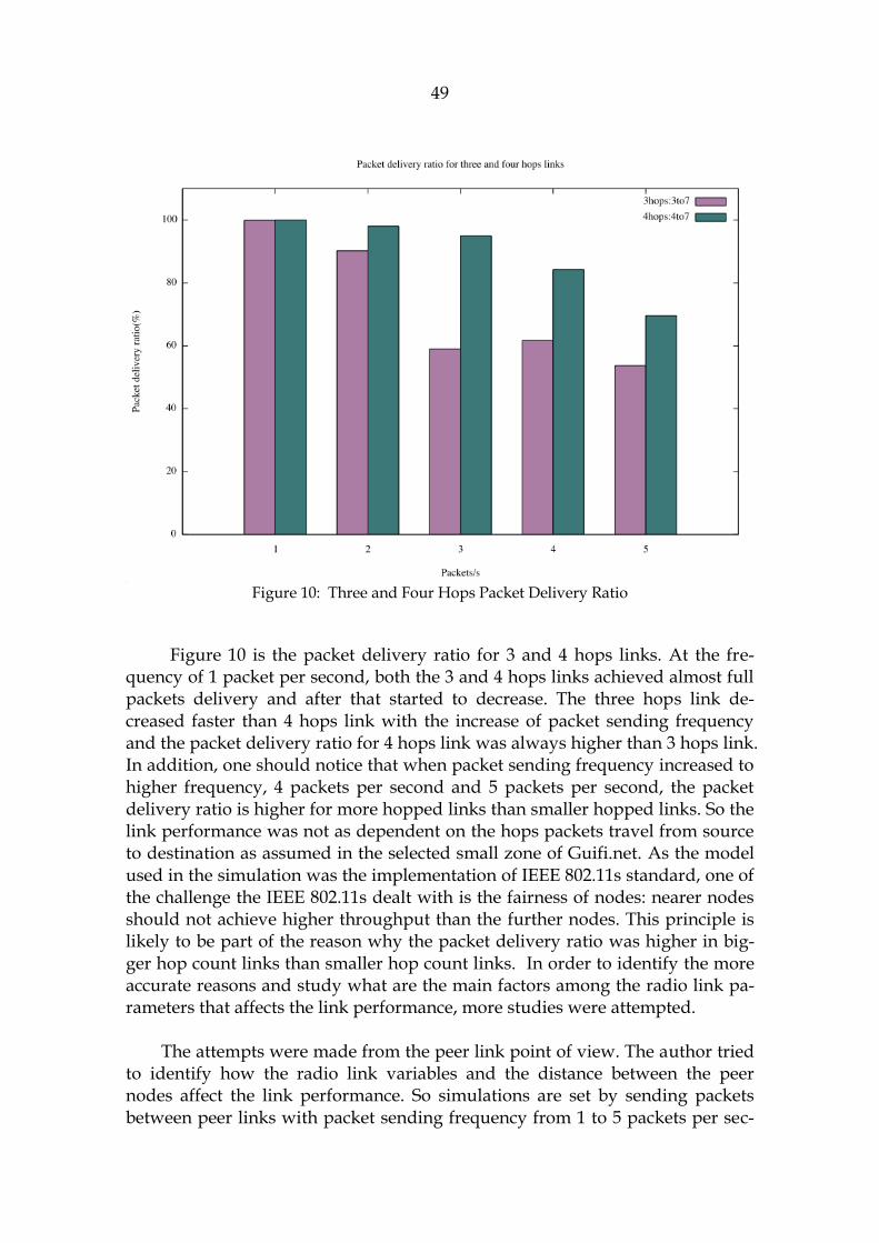
49

Figure 10: Three and Four Hops Packet Delivery Ratio

Figure 10 is the packet delivery ratio for 3 and 4 hops links. At the fre-quency of 1 packet per second, both the 3 and 4 hops links achieved almost full packets delivery and after that started to decrease. The three hops link de-creased faster than 4 hops link with the increase of packet sending frequency and the packet delivery ratio for 4 hops link was always higher than 3 hops link. In addition, one should notice that when packet sending frequency increased to higher frequency, 4 packets per second and 5 packets per second, the packet delivery ratio is higher for more hopped links than smaller hopped links. So the link performance was not as dependent on the hops packets travel from source to destination as assumed in the selected small zone of Guifi.net. As the model used in the simulation was the implementation of IEEE 802.11s standard, one of the challenge the IEEE 802.11s dealt with is the fairness of nodes: nearer nodes should not achieve higher throughput than the further nodes. This principle is likely to be part of the reason why the packet delivery ratio was higher in big-ger hop count links than smaller hop count links. In order to identify the more accurate reasons and study what are the main factors among the radio link pa-rameters that affects the link performance, more studies were attempted. The attempts were made from the peer link point of view. The author tried to identify how the radio link variables and the distance between the peer nodes affect the link performance. So simulations are set by sending packets between peer links with packet sending frequency from 1 to 5 packets per sec-

50

ond. Table 3 presents the simulation results (throughput in kbps of each link) with peer node distance, the antenna beam width and antenna transmission gain of the source node.

Peer link

Dis-tance (kilo -meter)

An-tenna beam width (de-gree)

An-tenna Tx Gain

1 p/s 2ps/s 3ps/s 4ps/s 5ps/s

5-4 0.185 30 18 4004.91 8004.68 12004.4 14337.1 14336.7

7-9 0.2497 360 14 4001.82 8002.94 12003.4 14369.2 14371.1

3-2 0.3073 360 14 4002.42 8002.88 12003.6 14362.6 14362.7

6-3 0.3739 30 14 4002.86 8003.35 12003.6 14320.8 14320.5

5-10 0.388 30 18 4003.94 8003.73 12003.5 14343.5 14343.3

7-8 0.3993 20 14 4000.34 8000.5 12000.7 14347.5 14347.8

1-7 0.6731 120 14 4000.81 8000.79 12000.8 14348.7 14349.5

5-6 1.0267 30 18 4001.91 8002.34 12002.8 14366.2 14366.7

7-5 1.4437 30 24 4009.2 8010.9 12012.6 14341.4 14341.7

0-1 1.4637 6 22 4002.99 8002.84 12002.7 14344.4 14344.4

Table 3: Distance, Radio Parameters and Throughput

According to the table, the throughput of each link with same packets sending frequency is very similar to each other, but still there are differences. When the packet sending frequencies are 1, 2 and 3 packets per second, the peer link throughput had minor decreases with the frequency increased. When the frequency increased from 4 to 5 packets per second, the throughput of the peer links did not increase. This might be an indication that with the radio settings in the selected zone of Guifi.net, the peer link cannot achieve higher application data rate, but this needs more approvals in the future studies. As the peer link throughput has similar patterns, where the throughput is slightly higher in the lower packet sending frequency, the throughput of same link is also higher in the higher packet sending frequency; the author took the throughput with 3 packets per second frequency for analysis. By calculating the correlations of peer link throughput and node distance, antenna beam width and antenna Tx gain, the author gained the results as fol-low:

Peer link throughput and antenna beam width: -0.10030378. Figure 11 shows the peer link throughput with different antenna beam width to-gether with the linear fitting curve y(x). As can be seen in the figure and the calculated correlation, the dependency of peer link throughput and the beam width of the transmission antenna are very low. With the as-

51

sumption that when the nodes are located more distantly, the antenna beam width should be in smaller degree in order to transmit to longer distance. The correlation of nodes distance and transmission antenna beam width is calculated and resulted in -0.32287. The result suggests that in the selected small zone of Guifi.net, the dependence of antenna beam width and the distance between the nodes is not high. However, the negative correlation partly approved the assumption of antenna beam width decreases as distance between nodes increases.

Figure 11: Antenna Beam Width and Throughput

Peer link throughput and node distance: -0.42061. Figure 12 presents the peer link throughput with different distance between the peer nodes and the linear fitting curve y(x). The figure and the calculated correlation suggest that the distance between the peer nodes increased, the through-put decreased. There are two exceptions: the two peer link with distance around 1.4 kilometers can achieve high throughput as the shorter dis-tance links.

Peer link throughput and antenna transmission gain: 0.692626. Figure 13 is the transmission gain of the transmitting antenna and the throughput of the peer link. The figure and calculated correlation suggest a positive correlation: with higher transmission gain of the antenna, the link can achieve higher throughput. However, the figure also suggests that even

52

with same antenna transmission gain, the peer link throughput can be different.

Referring back to Table 3 with careful investigation, the highest peer link throughput was achieved by link from node 7 to node 5 with the distance be-tween the nodes 1.4437 kilometers. The highlighting for this achievement is the transmission gain of the transmitting antenna at 24dBm. The peer links from node 5 to node 4, node 10 and node 6 resulted in different throughput. The in-fluencing factor is the distance between the nodes: nodes with longer distance resulted in smaller throughputs. The other peer links with the transmission gain at 14 dBm of the transmitting antenna, the throughput is affected by both the distance between the nodes and the antenna beam width.

Table 3 is rearranged with the analysis of the results of peer link study, as

Table 4. Referring to Table 4, the study on peer links indicates that the main in-fluencing factor on the peer link performance is the transmission gain of the transmitting antenna. The distance between the peer nodes has also considera-ble influence on the peer link performance. When other radio parameters are similar, antenna beam width can have some influence. In Table 4, the lowest throughput is from peer link node 7 to node 8. This link does not follow the de-scription above. The reason is the antenna orientation for this link is stored in the topology data, CNML file (the only link has antenna_azimuth attribute). The parsed antenna orientation is 0 degree which is not directed to node 8. The peer link from node 0 to node 1 did not achieve the proportionally higher throughput to the antenna transmission gain. The reason is the relatively far distance between the two nodes.

53

Figure 12: Node Distance and Throughput

Figure 13: Antenna Tx Gain and Throughput

54

Peer link

Tx Gain (dBm)

Dis-tance (km)

An-tenna beam width

Throughput(kbps) for different packet send-ing frequencies:

1 p/s 2 p/s 3 p/s 4 p/s 5 p/s

7-5 24 1.4437 30 4009.2 8010.9 12012.6 14341.4 14341.7

0-1 22 1.4637 6 4002.99 8002.84 12002.7 14344.4 14344.4

5-4 18 0.185 30 4004.91 8004.68 12004.4 14337.1 14336.7

5-10 18 0.388 30 4003.94 8003.73 12003.5 14343.5 14343.3

5-6 18 1.0267 30 4001.91 8002.34 12002.8 14366.2 14366.7

6-3 14 0.3739 30 4002.86 8003.35 12003.6 14320.8 14320.5

3-2 14 0.3073 360 4002.42 8002.88 12003.6 14362.6 14362.7

7-9 14 0.2497 360 4001.82 8002.94 12003.4 14369.2 14371.1

1-7 14 0.6731 120 4000.81 8000.79 12000.8 14348.7 14349.5

7-8 14 0.3993 20 4000.34 8000.5 12000.7 14347.5 14347.8

Table 4: Rearranged Peer Link Throughput

7.3 Other Analysis of the Topology Data

As presented in section 5.2, the CNML file is used in analysis in develop-ing the topology graph generator for Guifi.net. The CNML file contains the in-formation of the whole network, including the number of connections of the nodes and information on the radio links such as antenna beam width and so on. Such information can be used to develop abstract models of Guif.net. Petrov (2013) developed the topology generation scheme for Guifi.net. The developed topology generation algorithm can develop an abstract model of Guifi.net. Fig-ure 14 presents a possible topology graph of Gui.net model using the proposed algorithm introduced in Section 5.2 with desired 9 core nodes.

Based on the output graph, as Figure 14, of the topology graph generation

algorithm introduced in section 5.2, the numbers of core-to-core links and core-to-terminal links are known. Questions left are:

How many radio devices should be installed on each node?

Which antenna orientation and transmission gain should be assigned to the radio device?

How the nodes should be placed: the distance between the nodes?

55

Further statistics are done on the topology data including the antenna an-

gle (recall that the antenna angle attribute in the topology data stores the infor-mation for antenna beam width) distribution for the core nodes, the number of connection for devices with different numbers of antenna angles and the num-ber of core-to-core node connections for devices with different antenna angles.

Figure 14: Possible Topology Graph of Guifi.net

Figure 15 is the results of antenna angles distribution. From the figure, the antenna angles used for core nodes in Guifi.net is known: 6 degrees at about 23%, 30 degrees at about 36%, 60 degrees at about 2%, 90 degrees at about 5%, 120 degrees at about 32% and 360 degrees at about 4%.

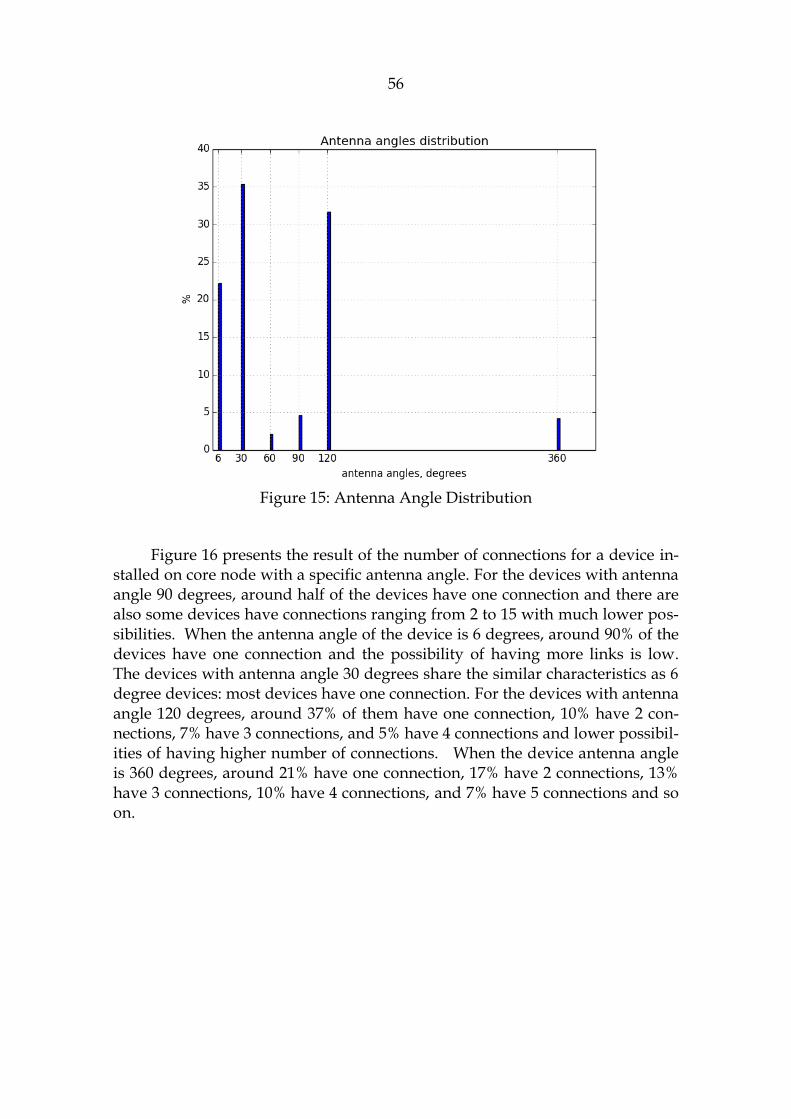
56

Figure 15: Antenna Angle Distribution

Figure 16 presents the result of the number of connections for a device in-stalled on core node with a specific antenna angle. For the devices with antenna angle 90 degrees, around half of the devices have one connection and there are also some devices have connections ranging from 2 to 15 with much lower pos-sibilities. When the antenna angle of the device is 6 degrees, around 90% of the devices have one connection and the possibility of having more links is low. The devices with antenna angle 30 degrees share the similar characteristics as 6 degree devices: most devices have one connection. For the devices with antenna angle 120 degrees, around 37% of them have one connection, 10% have 2 con-nections, 7% have 3 connections, and 5% have 4 connections and lower possibil-ities of having higher number of connections. When the device antenna angle is 360 degrees, around 21% have one connection, 17% have 2 connections, 13% have 3 connections, 10% have 4 connections, and 7% have 5 connections and so on.

57

Figure 16: Distribution of Number of Links per Device

Figure 17 shows the results of the number core-to-core node connections for a device with a specific antenna angle. When the device antenna angle is 90 degrees, 65% devices do not have core-to-core connection, around 28% have one core-to-core connection and much lower percentage have more core-to-core connections. For the devices with antenna angle 6 degrees, 55% devices do not have core-to-core links and 43% have one core-to-core link. The devices with antenna angle 30 degrees share similar characteristics as 6 degrees devices. When the antenna angle is 120 degress, around 80% do not have core-to-core link and 18% have one core-to-core link. Devices with antenna angle 360 de-grees share the similar pattern as 120 degree devices.

58

Figure 17: Distribution of Core-to-Core Links per Device

After having the statistical result, the topology generation can proceed forward. Among the known number of core nodes, which is the input parame-ter for the topology graph generation, one core node is taken under considera-tion first. For the core node under consideration, one net device is installed at first. And for the installed net device, the antenna angle is defined according to the probability distribution (with Figure 15). With the assigned antenna angle, referring to Figure 16 the probable total number of connections can be found including both core-to-core connections and core-to-terminal connections. Re-ferring to the results shown in Figure 17, the number of core-to-core connec-tions can be defined. And after this process, the first core-to-core link for the core node under consideration is set up. In case of links are left, more net de-vices are added to the node till all the links are build up. After all the links are considered, the connected nodes should be placed inside the antenna angle. The extract positions of the connected nodes are set according to the node dis-tance distribution. Then the antenna gains for the radio links are defined. The net devices should operate in different frequency bands to avoid collisions. When the links for one core node is set up, next core node is taken into consid-eration. This process continues till all the core nodes are considered. The ter-minal nodes which have only one net device are attached to the core node and placed inside the antenna angle.

59

8 CONCLUSION

In this thesis, the author studied the wireless mesh networks. A detailed under-standing of wireless mesh networks is gained, including the topology, the relat-ed routing protocols and the related standards. As a part of the early stage re-search on the topology generator for Guif.net, the author also studied the topol-ogy data of Guifi.net stored in CNML and used the data to model a small zone of Guifi.net. The critical data stored in CNML for modelling Guifi.net includes the node position and some radio link related data such as antenna beam width, antenna azimuth, the channel frequency and the antenna transmission gain. Performance study on the modeled small zone was done by the simulations using NS-3 as a tool. The author gained a deep understanding of the selected zone. First, with higher application data rate (more frequent packets sending) the network efficiency decreased which is shown on the lowered packet deliv-ery ratio and not increased network throughput. Second, with high application data rate, the end-to-end delays of the packets are considerately enlarged. This indicates that the network do not have good performance in providing high data rate services such as VoIP, video and so on. Third, the packet delivery ratio and the hop count are not dependent on each other in the specific simulation scenario. Fourth, the key influence factors for the peer links in the modeled small zone of Guif.net are the antenna transmission gain and the distance be-tween the nodes. Antenna beam width affects the peer link performance when other radio link parameters are similar. The topology generation scheme for Guifi.net is also studied carefully and presented at the end of the thesis.

In the future, the modeling of Guifi.net using the existing topology data

should be carried out in larger scales since the study in this thesis used only very limited amount of data stored in CNML. Thus, the performance study re-sults are only valid in the selected small zone. Whether the results of the per-formance study is also valid for other zones (either similar sized or larger ones) should be approved via more studies. From the further studies, some questions should be answered: do zones in Guifi.net share the same performance charac-teristics and same influencing factors on peer links? Or the zones share different

60

patterns but can be grouped and so on. In this thesis study, the IEEE 802.11s implementation in NS-3 was used. The further studies should also include studies that use IP layer routing protocols such as OLSR, since OLSR is used in some part of Guifi.net. One other future work approach is continuing develop-ing the topology generation scheme for Guifi.net: first continuing from the ana-lytical studies, for example the node distance distributions, and eventually complete the topology generation scheme. Simulations can be used as a validat-ing tool. The understanding of more accurate performance patterns of Guifi.net can provide good bases for the simulation studies for the topology generation scheme. These further studies on Guifi.net should be able to contribute back to Guifi.net by identifying the topology impact on the network performance, iden-tifying the critical variables in the radio link settings and suggesting the selec-tion of proxy nodes, radio service provider nodes, gaming service provider nodes, and VoIP service provider nodes and so on. As for the wireless mesh networks in general, the future networks are moving toward energy efficient, self-organized intelligent networks. Further researches could be done in the development of wireless mesh networks that are self-managed intelligently in a distributed fashion.

61

62

REFERENCES

Afanasyev, M., Chen, T., Voelker, G. and Snoeren, A. (2010) Usage Patterns in an Urban WiFi Network. IEEE/ACM Transaction on Networking (TON), 18(5), 1359-1372

Aguayo, D. et al. (2004) Link-level Measurements from an 802.11b Mesh Network. ACM SIGCOMM Computer Communication Review, 34(4), 121-132

Akildiz, I. and Wang, X. 2009. Wireless Mesh Networks. Hoboken, NJ:J.Wiley and Sons.

Akyildiz, I. and Wang, X (2005) A Survey on Wireless Mesh Networks. IEEE Communication Magazine, 43(9), 23-30

Bicket, J. et al. (2005) Architecture and Evaluation of an Unplanned 802.11b mesh network. 11th Annual International Conference On Mobile Computing And Networking, ACM, 31-42

Boukerche, A. (2004) Performance Evaluation of Routing Protocols for ad hoc Wireless Networks. Mobile Networks And Applications 9(4), 333

Brik, V. et al. ( 2008) A Measurement Study of a Commercial-grade Urban WIFI Mesh. 8th ACM SIGCOMM Conference On Mobile Computing And Netowrking, 74-85

Bruno, R., Conti, M. and Gregori, E. (2005) Mesh Networks: Commodity Multihop Ad Hoc Networks. IEEE Communication Magazine, 123-131

Calcada, T., Cortez, P. and Ricardo, M. (2012) Using Data Mining to Study the Impact of Topology Characteristics on the Performance of Wireless Mesh Networks. Wireless Communications and Networking Conference (WCNC), 2012 IEEE. 1725-1730

63

Camp, J., Knightly,E. (2008) “The IEEE 802.11s Extended Service Set Mesh Networking Standard”, IEEE Communication Magazine, 46(8), 120-125

Carrano, R.C., Magalhaes, L.C.S, Muchalau Saade, D.C., and Albuquerque, C.V.N. (2011) IEEE 802.11s Multihop MAC: A Tutorial”. IEEE Communications Survey & Tutorials, 13(1), 52-67

Cerdà-Alabern, L. (2012) On The Topology Characterization Of Guifi.Net. International Conference on Wireless and Mobile Computing, Networking an Communications, 389-396

CIER Deliverables. Based on personal communications with the supervisors

Efstathiou, E., Frangoudis, P. and Polyzos, G. (2006) Stimulating Participation In Wieless Community Networks. IEEE INFOCOM, 6

Faccin, S., Wijting, C., Kneckt, J. and Damle, A. (2006) Mesh WLAN Network: Concept and System Design. IEEE Wireless Communications, 10-17

Fu, Y. (2013) Research of Wireless Mesh Network Performance Based on NSTUns. 2013 Fifth International Conference on Computational and Information Sciences (ICCIS). 1339-1342

Gerla, M., Chen, T. and Pei, G. (2000) Fisheye State Routing : A Routing Scheme For Ad Hoc Networks. IEEE International Conference on Communications,1, 70-74

Gregor, S. (2006) The Nature of Theory in Information Systems. MIS Quaterly 30(3), 611-642

64

Gupta, P. and Gupta, S. (2013) Performance Evaluation of Mobility Models on MANET Routing Protocols. Third International Conference on Advanced Computing and Communication Technologies (ACCT).248-253

Heirtz,G.R. et al. (2010) IEEE 802.11s: The WLAN Standard. IEEE Wireless Communications, 104-111

Held, G. (2005) Wireless Mesh Networks. Auerbach Publications.

IEEE Standard For Information Technology, Telecommunications And Information Exchange Between Systems, Local And Metropolitan Area Networks, Specific Requirements, Part 11: Wireless LAN Medium Access Control (MAC) And Physical Layer (PHY) Specifications, Amendment 10: Mesh Networking, IEEE Computer Society, IEEE STD 802.11s (2011), New York

Kasanen, E., Lukka, K. and Siitonen A. (1993) The Constructive Approach in Management Accouting Research. Journal of Management Accounting Research, 5, 243-263

Kumar, S. and Kumar, J. (2012) Comparative Analysis Of Proactive And Reactive Routing Protocols In Mobile Ad-Hoc Networks (MANET). Journal Of Information And Operations Management 3(1) 92-95

LaCurt, K. and Balakrishnan, H. (2010) Measurement And Analysis Of Real-World 802.11 Mesh Networks. 10th Annual Conference On Internet Measurement, ACM, 187-198

Lindholm, A-L. (2008) A Constructive Study on Creating Core Business Relevant CREM Strategy and Performance Measures. Facilities 26(7/8), 343

Liu, F. and Bai, Y. (2012) An Overview Of Topology Control Mechanisms In Multi-Radio Multi-Channel Wireless Mesh Networks. EURASIP Journal on Wireless Communications and Networking

65

Ma, C. and Yang,Y.(2007) A Battery Aware Scheme for Energy Efficient Coverage and Routing in Wireless Mesh Networks. IEEE, Global Telecommunication Conference, GLOBECOM’07

Molle, C. and Voge, M-E. (2010) A Quantitative Analysis Of The Capacity Of Wireless Mesh Networks. IEEE Communication Letters, 14(5), 438-440

Natkaniec, M. (2009) Ad Hoc Mobile Wireless Networks: Principles, Protocols and Applications (Sarkar, S. K. et al, 2008) [Book Review]. IEEE Communication Magazine 20090101 47(5), 12

Petrov, D. (2013) Topology Generation Scheme. Based on personal communication.

Piirainen, K.A. and Gonzalez R.A. (2013) Seeking Constructive Synergy: Design Science and he Constructive Research Approach. Design Science at the Intersection of Physical and Virtual Design, 59-72

Rabbi, M.F. (2006) An Efficient Wireless Mesh Network: A New Architecture. International Conference on Communication Technology, 1-5

Shah, K., Fransesco, M.D. and Kumar, M. (2013) Distributed Resource Management in Wireless Sensor Networks Using Reinforcement Learning. Wireless Networks, 19(5), 705-724.

Singer, B.P. et al ( 2007) Corporate Real Estate and Competitive Strategy. Journal of Corporate Real Estate 9(1), 25

Siris, V.A., Tragos, E.Z. and Petroulakis, N.E. (2012) Experiences With A Metropolitan Multiradio Wireless Mesh Network: Design, Performance, And Application. IEEE Communication Magazine, 50(7), 128-136

66

Szabó, C., Horváth, Z. and Farkas, K. (2007) Wireless Community Networks: Motivations, Design And Business Models. 3rd international conference on wireless internet. ICST(Institute for Computer Sciences, Social-Infomatics and Telecommunications Engineering). 23

Tan, K., Wu, D., Chan, A. and Mohapatra, P. (2011) Comparing Simulation Tools And Experimental Testbeds For Wireless Mesh Networks. Pervasive and Mobile Computing, 7(4), 434-443

Valle, De T. et al. (2008) Mesh Topology Viewer (MTV): An SVG-based Interactive Mesh Network Topology Visualization Tool. IEEE Symposium on Comuters and Communications, 292-297

Vega, D., Cerdà-Alabern, L., Navarro, L. and Meseguer, R. (2012) Topology Patterns Of A Community Network: Guifi.net. International Conference on Wireless and Mobile Computing, Networking and Communications, 612-619

Wang, X. and Lim, A.O. (2007) IEEE802.11s Wireless Mesh Networks: Framework And Challenges. Ad Hoc Networks

Yu, Z., Xu, X. and Wu, X. (2010) Application Of Wireless Mesh Network In Campus Network. Second International Conference On Communication Systems Networks And Applications IEEE, 245-247.

Andreev,K. and Boiko,P. (2009) IEEE 802.11s Mesh Networking NS-3 Model retrieved from: http://www.nsnam.org/workshops/wns3-2010/dot11s.pdf

CNML, Guifi.Net Retrieved on 23.6.2013 from http://en.wiki.guifi.net/wiki/CNML

Guifi.net, “Open, Free and Neutral Network Internet for everybody”, http://guifi.net/en

67

One Laptop per Child, About the Project. Retrieved from http://one.laptop.org/about/mission on 16.2.2014

FunkFeuer. Retrieved on 19.9.2013 from http://www.funkfeuer.at/Home.42.0.html?&L=1

Hospitalet de Llobregat, L’, Guifi.Net Retrieved on 31.01.2014 from http://guifi.net/en/node/3988/view/services

IEEE802.15.5 Bluetooth. Retrieve on 13.11.2013 from http://standards.ieee.org/getieee802/download/802.15.5-2009.pdf

IEEE802.15.4 Zigbee. Retrieved on 13.11.2013 from

http://staff.ustc.edu.cn/~ustcsse/papers/SR10.ZigBee.pdf

LogDistancePathLossModel, ns-3. Retrieve on 9.1.2014 from http://www.nsnam.org/doxygen-release/classns3_1_1_log_distance_propagation_loss_model.html#details

Lukka, K.(2002). Konstruktiivinen Tutkimusote. Retrieved 26.08.2013, from http://www.metodix.com/en/sisallys/04_virtuaalikirjasto/dokumentit/aineistot/konstruktiivinentutkimusote

Mesh Device, ns-3 Retrieve on 7.1.2014 from http://www.nsnam.org/doxygen/group__mesh.html

MeshHelper Class Reference Retrieved on 13.01.2013 from https://www.nsnam.org/doxygen-release/classns3_1_1_mesh_helper.html

New Orleans Wi-Fi Network. Retrieved on 19.9.2013 from http://www.computerworld.com/s/article/109662/New_Orleans_Wi_Fi_network_now_a_lifeline

68

NS-3, “what is ns-3” Retrieved 13.08.2013 from: http://www.nsnam.org/overview/what-is-ns-3/

NS-3 Tutorial. Retrieved 20.11.2013 from: http://www.nsnam.org/docs/release/3.18/tutorial/singlehtml/index.html#document-conceptual-overview

OnOff Application, NS-3. Retrieve on 28.11.2013 from http://www.nsnam.org/docs/release/3.16/doxygen/classns3_1_1_on_off_application.html

Perkins, C., Belding-Royer, E. and Das, S. (2003) Ad hoc On-DemandDistance Vector (AODV) Routing. Request for Comments (Experimental) 3561, July 2003, Retrieved from: http://www.ietf.org/rfc/rfc3561.txt.

RoofNet-Introduction. Retrived on 16.2.2014 from http://www.comclub.org/roofnet/

San Mateo Police Department Adopts Wi-Fi. Retrieved on 19.9.2013 from http://www.govtech.com/security/San-Mateo-Police-Department-Adopts-Wi-Fi.html

69

ATTACHMENT S

Attachment 1: Python Script for Parsing the CNML File Used in Studying the Small Zone

__version__ = 1.0 __author__ = "Dmitry Petrov <dmit-

ry.petrov@magister.fi>" __license__ = "GNU GPLv3+" import xml.dom.minidom as MD import sys import ast from math import cos, sin, tan, atan def completeArbol(cnmlFile): try: tree = MD.parse(cnmlFile) except IOError: print( "CNML file \"%s\" couldn't be

ed" %cnmlFile) return zones = tree.getElementsByTagName("zone") zone = findZone("3988", zones) coreNodesStat(zone) #n_subzones = len(z.getElementsByTagName("zone")) #print("NUmber of subzones ", n_subzones) #nodes = z.getElementsByTagName("node") #n_nodes = simpleNodescount(nodes) #if n_subzones > 0: # parent.append(n_nodes) def coreNodesStat(zone): f1 = open('out\\guifi3988az.dat', 'w+') f1.write("nodeID\tlinked\tAntenna\tGain\tChannel\n

") nodes = zone.getElementsByTagName("node")

70

for n in nodes: st = n.getAttribute("status") if st == "Working": id=n.getAttribute("id") device=n.getElementsByTagName("device") for d in device: radios=d.getElementsByTagName("radio") for radio in radios: azi-

muth=radio.getAttribute("antenna_azimuth") if azimuth != " ": angles=azimuth elif azimuth == " ": angles=1 gain=radio.getAttribute("antenna_gain") channel=radio.getAttribute("channel") inter-

face=radio.getElementsByTagName("interface") for i in interface: links=i.getElementsByTagName("link") for link in links: linked

=link.getAttribute("linked_node_id") stat=id stat+="\t" stat+= "angle"+angles stat+="\t" stat+= "gain"+gain stat+="\t" stat+= "channel"+channel stat+="\t" stat+="|"+linked+"|" stat+="\n" f1.write(stat)

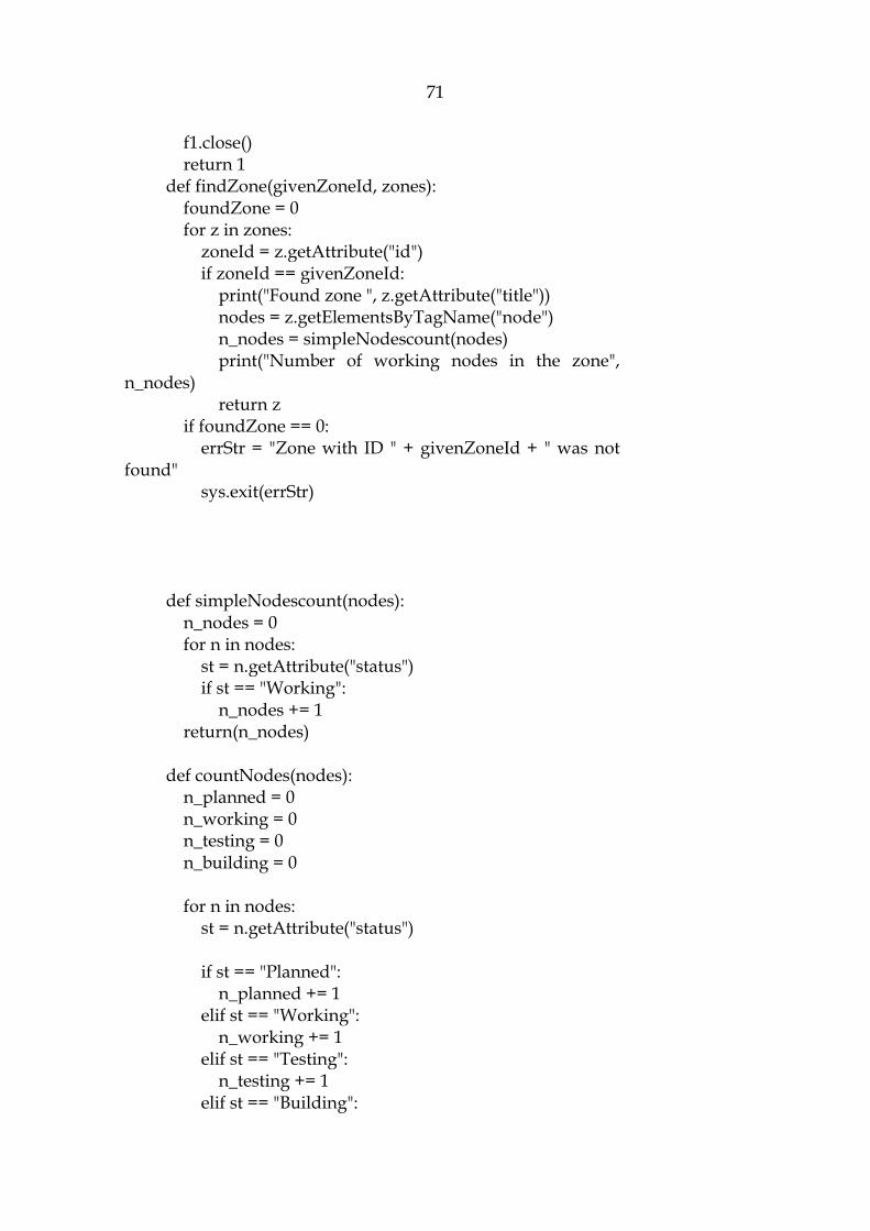
71

f1.close() return 1 def findZone(givenZoneId, zones): foundZone = 0 for z in zones: zoneId = z.getAttribute("id") if zoneId == givenZoneId: print("Found zone ", z.getAttribute("title")) nodes = z.getElementsByTagName("node") n_nodes = simpleNodescount(nodes) print("Number of working nodes in the zone",

n_nodes) return z if foundZone == 0: errStr = "Zone with ID " + givenZoneId + " was not

found" sys.exit(errStr) def simpleNodescount(nodes): n_nodes = 0 for n in nodes: st = n.getAttribute("status") if st == "Working": n_nodes += 1 return(n_nodes) def countNodes(nodes): n_planned = 0 n_working = 0 n_testing = 0 n_building = 0 for n in nodes: st = n.getAttribute("status") if st == "Planned": n_planned += 1 elif st == "Working": n_working += 1 elif st == "Testing": n_testing += 1 elif st == "Building":

72

n_building += 1 else: print("Unknown node status: ", st) # Working, Building, Testing, Planned. return (n_working, n_building, n_testing, n_planned) def TestFun(): print('Hui') def main(): TestFun() cnmlFile = 'guifi.cnml' completeArbol(cnmlFile) # Standard boilerplate to call the main() function to begin # the program. if __name__ == '__main__': main() #f = open('test.dat', 'w+') #f.write('This is a test\n') #from elementtree import ElementTree as et #f2 = open('guifi.cnml', 'r+') #tree = et.fromstring(f2) #nodeI = 0 # iterate over the dict elements #for node_el in tree.iterfind('node'): # nodeI = nodeI+1 #f.write ('asdfsadfasd\n') #f.write (str(nodeI)) #f.close ()

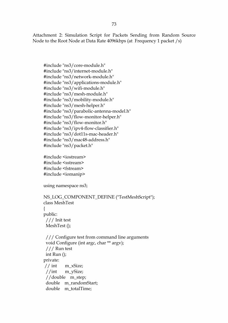
73

Attachment 2: Simulation Script for Packets Sending from Random Source Node to the Root Node at Data Rate 4096kbps (at Frequency 1 packet /s)

#include "ns3/core-module.h" #include "ns3/internet-module.h" #include "ns3/network-module.h" #include "ns3/applications-module.h" #include "ns3/wifi-module.h" #include "ns3/mesh-module.h" #include "ns3/mobility-module.h" #include "ns3/mesh-helper.h" #include "ns3/parabolic-antenna-model.h" #include "ns3/flow-monitor-helper.h" #include "ns3/flow-monitor.h" #include "ns3/ipv4-flow-classifier.h" #include "ns3/dot11s-mac-header.h" #include "ns3/mac48-address.h" #include "ns3/packet.h" #include <iostream> #include <sstream> #include <fstream> #include <iomanip> using namespace ns3; NS_LOG_COMPONENT_DEFINE ("TestMeshScript"); class MeshTest { public: /// Init test MeshTest (); /// Configure test from command line arguments void Configure (int argc, char ** argv); /// Run test int Run (); private: // int m_xSize; //int m_ySize; //double m_step; double m_randomStart; double m_totalTime;

74

double m_packetInterval; uint16_t m_packetSize; //uint32_t m_nIfaces; bool m_chan; bool m_pcap; std::string m_stack; std::string m_root; /// List of network nodes NodeContainer nodes; /// List of all mesh point devices NetDeviceContainer meshDevices; //Addresses of interfaces: Ipv4InterfaceContainer interfaces; // MeshHelper. Report is not static methods MeshHelper mesh; private: /// Create nodes and setup their mobility void CreateNodes (); /// Install internet m_stack on nodes void InstallInternetStack (); void AddAntennas(); /// Install applications void InstallApplication (); /// Print mesh devices diagnostics void Report (); Ptr<Socket> SetupPacketReceive(Ipv4Address addr, Ptr<Node> node); void ReceivePacket(Ptr<Socket> socket); uint32_t port; uint32_t packetsReceived; uint32_t bytesTotal; }; MeshTest::MeshTest () : m_randomStart (0.1), m_totalTime (100.0), m_packetInterval (0.1), m_packetSize (512), //m_nIfaces (2), m_chan (true), m_pcap (false), m_stack ("ns3::Dot11sStack"), port(9), packetsReceived(0), bytesTotal(0) { }

75

std::string PrintReceivedPacket (Ptr<Socket> socket, Ptr<Packet> packet) { SocketAddressTag tag; bool found; found = packet->PeekPacketTag (tag); std::ostringstream oss; oss << Simulator::Now ().GetSeconds () << " " << socket->GetNode ()-

>GetId (); if (found) { InetSocketAddress addr = InetSocketAddress::ConvertFrom

(tag.GetAddress ()); oss << " received one packet from " << addr.GetIpv4 (); } else { oss << " received one packet!"; } return oss.str (); } void MeshTest::ReceivePacket (Ptr<Socket> socket) { Ptr<Packet> packet; while ((packet = socket->Recv ())) { bytesTotal += packet->GetSize (); packetsReceived += 1; //NS_LOG_UNCOND (PrintReceivedPacket (socket, packet)); } } Ptr<Socket> MeshTest::SetupPacketReceive (Ipv4Address addr, Ptr<Node> node) { TypeId tid = TypeId::LookupByName ("ns3::UdpSocketFactory"); Ptr<Socket> sink = Socket::CreateSocket (node, tid); InetSocketAddress local = InetSocketAddress (addr, port); sink->Bind (local); sink->SetRecvCallback (MakeCallback (&MeshTest::ReceivePacket,

76

this)); return sink; } void MeshTest::Configure (int argc, char *argv[]) { CommandLine cmd; /* * As soon as starting node means that it sends a beacon, * simultaneous start is not good. */ cmd.AddValue ("start", "Maximum random start delay, seconds. [0.1 s]",

m_randomStart); cmd.AddValue ("time", "Simulation time, seconds [100 s]", m_totalTime); cmd.AddValue ("packet-interval", "Interval between packets in UDP

ping, seconds [0.001 s]", m_packetInterval); cmd.AddValue ("packet-size", "Size of packets in UDP ping",

m_packetSize); cmd.AddValue ("channels", "Use different frequency channels for dif-

ferent interfaces. [0]", m_chan); cmd.AddValue ("pcap", "Enable PCAP traces on interfaces. [0]",

m_pcap); cmd.AddValue ("stack", "Type of protocol stack. ns3::Dot11sStack by de-

fault", m_stack); //cmd.AddValue ("root", "Mac address of root mesh point in HWMP",

m_root); cmd.Parse (argc, argv); NS_LOG_DEBUG ("Simulation time: " << m_totalTime << " s"); } void MeshTest::CreateNodes () { nodes.Create (11); // Configure YansWifiChannel YansWifiPhyHelper wifiPhy = YansWifiPhyHelper::Default (); YansWifiChannelHelper wifiChannel ; //setpropagationdelay and loss wifiChannel.SetPropagationDelay

("ns3::ConstantSpeedPropagationDelayModel");

77

wifiChannel.AddPropagationLoss ("ns3::LogDistancePropagationLossModel","Exponent",

StringValue ("2.7")); wifiPhy.SetChannel (wifiChannel.Create ()); //can configure the parameters of peer management protocol //and HWMP parameters also /* * Create mesh helper and set stack installer to it * Stack installer creates all needed protocols and install them to * mesh point device */ mesh = MeshHelper::Default (); mesh.SetStandard(WIFI_PHY_STANDARD_80211a); mesh.SetRemoteStationManager("ns3::ConstantRateWifiManager",

"DataMode",StringValue("OfdmRate54Mbps"));//threshold can be set here also //proactive mode, set root node to 6149 m_root = "00:00:00:00:00:12";//mac address of interface 5 of node 7 mesh.SetStackInstaller(m_stack, "Root",

Mac48AddressValue(Mac48Address(m_root.c_str()))); if (m_chan) { mesh.SetSpreadInterfaceChannels (MeshHelp-

er::SPREAD_CHANNELS); } else { mesh.SetSpreadInterfaceChannels (MeshHelper::ZERO_CHANNEL); } mesh.SetMacType ("RandomStart", TimeValue (Seconds

(m_randomStart))); // Set number of interfaces - default is single-interface mesh point //36118 mesh.SetNumberOfInterfaces (1); // Install protocols and return container if MeshPointDevices meshDevices = mesh.Install (wifiPhy, nodes.Get(0)); //29243 mesh.SetNumberOfInterfaces (2); // Install protocols and return container if MeshPointDevices meshDevices.Add(mesh.Install (wifiPhy, nodes.Get(1)));

78

//34529 mesh.SetNumberOfInterfaces (1); // Install protocols and return container if MeshPointDevices meshDevices.Add(mesh.Install (wifiPhy, nodes.Get(2))); //5975 mesh.SetNumberOfInterfaces (2); // Install protocols and return container if MeshPointDevices meshDevices.Add(mesh.Install (wifiPhy, nodes.Get(3))); //5737 mesh.SetNumberOfInterfaces (1); // Install protocols and return container if MeshPointDevices meshDevices.Add(mesh.Install (wifiPhy, nodes.Get(4))); //5738 mesh.SetNumberOfInterfaces (4); // Install protocols and return container if MeshPointDevices meshDevices.Add(mesh.Install (wifiPhy, nodes.Get(5))); //15247 mesh.SetNumberOfInterfaces (2); // Install protocols and return container if MeshPointDevices meshDevices.Add(mesh.Install (wifiPhy, nodes.Get(6))); //6149 mesh.SetNumberOfInterfaces (5);//one interface is the proxy // Install protocols and return container if MeshPointDevices meshDevices.Add(mesh.Install (wifiPhy, nodes.Get(7))); //32520 mesh.SetNumberOfInterfaces (1); // Install protocols and return container if MeshPointDevices meshDevices.Add(mesh.Install (wifiPhy, nodes.Get(8))); //14733 mesh.SetNumberOfInterfaces (1); // Install protocols and return container if MeshPointDevices meshDevices.Add(mesh.Install (wifiPhy, nodes.Get(9))); //7996 mesh.SetNumberOfInterfaces (1); // Install protocols and return container if MeshPointDevices meshDevices.Add(mesh.Install (wifiPhy, nodes.Get(10))); // Setup mobility - static grid topology //locate nodes Ptr<ns3::ListPositionAllocator>PosAlloc=CreateObject<ns3::ListPosition

Allocator>(); MobilityHelper mobility; //36118 0 PosAlloc->Add(Vector(0.0,0.0,0.0));

79

//29243 1 PosAlloc->Add(Vector(1.265844,-0.734825,0.0)); //34529 2 PosAlloc->Add(Vector(0.898545,-1.2257, 0.0)); //5975 3 PosAlloc->Add(Vector(0.954933,-1.52779, 0.0)); //5737 4 PosAlloc->Add(Vector(1.018314,-2.391135, 0.0)); //5738 5 PosAlloc->Add(Vector(1.070262,-2.21357, 0.0)); //15274 6 PosAlloc->Add(Vector(1.110222,-1.18762, 0.0)); //6149 7 PosAlloc->Add(Vector(1.877232,-1.01643, 0.0)); //32520 8 PosAlloc->Add(Vector(2.259738,-0.901765, 0.0)); //14733 9 PosAlloc->Add(Vector(2.021754,-0.812855, 0.0)); //7996 10 PosAlloc->Add(Vector(1.363191,-2.467975, 0.0)); mobility.SetPositionAllocator(PosAlloc); mobility.SetMobilityModel("ns3::ConstantPositionMobilityModel"); mobility.Install (nodes); if (m_pcap) wifiPhy.EnablePcapAll (std::string ("mp-")); } void MeshTest::InstallInternetStack () { InternetStackHelper internetStack; internetStack.Install (nodes); Ipv4AddressHelper address; address.SetBase ("10.1.1.0", "255.255.255.0"); interfaces = address.Assign (meshDevices); } void MeshTest::AddAntennas() { for(NetDeviceContainer::Iterator

i=meshDevices.Begin();i<meshDevices.End();i++) { uint32_t intN=(*i)->GetObject<MeshPointDevice>()-

80

>GetNInterfaces(); for(uint32_t n=0;n<intN;n++) { Ptr<ParabolicAntennaModel> anten-

na=CreateObject<ParabolicAntennaModel>(); (*i)->GetObject<MeshPointDevice>()->GetInterfaces()[n]-

>GetObject<WifiNetDevice>()->AggregateObject(antenna); } } //look the graph and set a suitable antenna orientation meshDevices.Get(0)->GetObject<MeshPointDevice>()->GetInterface(1)-

>GetObject<WifiNetDevice>()->GetObject<ParabolicAntennaModel>()->SetBeamwidth(6.0);

meshDevices.Get(0)->GetObject<MeshPointDevice>()->GetInterface(1)->GetObject<WifiNetDevice>()->GetObject<ParabolicAntennaModel>()->SetOrientation(300.0);

meshDevices.Get(0)->GetObject<MeshPointDevice>()->GetInterface(1)->GetObject<WifiNetDevice>()->GetPhy()->GetObject<YansWifiPhy>()->SetTxGain(22.0);

meshDevices.Get(0)->GetObject<MeshPointDevice>()->GetInterface(1)->GetObject<WifiNetDevice>()->GetPhy()->SetChannelNumber(112);

meshDevices.Get(1)->GetObject<MeshPointDevice>()->GetInterface(1)-

>GetObject<WifiNetDevice>()->GetObject<ParabolicAntennaModel>()-> Set-Beamwidth(120.0);

meshDevices.Get(1)->GetObject<MeshPointDevice>()->GetInterface(1)->GetObject<WifiNetDevice>()->GetObject<ParabolicAntennaModel>()-> SetOrientation(315.0);

meshDevices.Get(1)->GetObject<MeshPointDevice>()->GetInterface(1)->GetObject<WifiNetDevice>()->GetPhy()->GetObject<YansWifiPhy>()->SetTxGain(14.0);

meshDevices.Get(1)->GetObject<MeshPointDevice>()->GetInterface(1)->GetObject<WifiNetDevice>()->GetPhy()->SetChannelNumber(132);

meshDevices.Get(1)->GetObject<MeshPointDevice>()->GetInterface(2)-

>GetObject<WifiNetDevice>()->GetObject<ParabolicAntennaModel>()->SetBeamwidth(30.0);

meshDevices.Get(1)->GetObject<MeshPointDevice>()->GetInterface(2)->GetObject<WifiNetDevice>()->GetObject<ParabolicAntennaModel>()->SetOrientation(150.0);

meshDevices.Get(1)->GetObject<MeshPointDevice>()->GetInterface(2)->GetObject<WifiNetDevice>()->GetPhy()->GetObject<YansWifiPhy>()->SetTxGain(23.0);

meshDevices.Get(1)->GetObject<MeshPointDevice>()->GetInterface(2)->GetObject<WifiNetDevice>()->GetPhy()->SetChannelNumber(112);

81

meshDevices.Get(2)->GetObject<MeshPointDevice>()->GetInterface(1)-

>GetObject<WifiNetDevice>()->GetObject<ParabolicAntennaModel>()->SetBeamwidth(30.0);

meshDevices.Get(2)->GetObject<MeshPointDevice>()->GetInterface(1)->GetObject<WifiNetDevice>()->GetObject<ParabolicAntennaModel>()->SetOrientation(280.0);

meshDevices.Get(2)->GetObject<MeshPointDevice>()->GetInterface(1)->GetObject<WifiNetDevice>()->GetPhy()->GetObject<YansWifiPhy>()->SetTxGain(12.0);

meshDevices.Get(2)->GetObject<MeshPointDevice>()->GetInterface(1)->GetObject<WifiNetDevice>()->GetPhy()->SetChannelNumber(8);

meshDevices.Get(3)->GetObject<MeshPointDevice>()->GetInterface(1)-

>GetObject<WifiNetDevice>()->GetObject<ParabolicAntennaModel>()->SetBeamwidth(360.0);

meshDevices.Get(3)->GetObject<MeshPointDevice>()->GetInterface(1)->GetObject<WifiNetDevice>()->GetObject<ParabolicAntennaModel>()->SetOrientation(100.0);

meshDevices.Get(3)->GetObject<MeshPointDevice>()->GetInterface(1)->GetObject<WifiNetDevice>()->GetPhy()->GetObject<YansWifiPhy>()->SetTxGain(14.0);

meshDevices.Get(3)->GetObject<MeshPointDevice>()->GetInterface(1)->GetObject<WifiNetDevice>()->GetPhy()->SetChannelNumber(8);

meshDevices.Get(3)->GetObject<MeshPointDevice>()->GetInterface(2)-

>GetObject<WifiNetDevice>()->GetObject<ParabolicAntennaModel>()->SetBeamwidth(30.0);

meshDevices.Get(3)->GetObject<MeshPointDevice>()->GetInterface(2)->GetObject<WifiNetDevice>()->GetObject<ParabolicAntennaModel>()->SetOrientation(60.0);

meshDevices.Get(3)->GetObject<MeshPointDevice>()->GetInterface(2)->GetObject<WifiNetDevice>()->GetPhy()->GetObject<YansWifiPhy>()->SetTxGain(14.0);

meshDevices.Get(3)->GetObject<MeshPointDevice>()->GetInterface(2)->GetObject<WifiNetDevice>()->GetPhy()->SetChannelNumber(128);

meshDevices.Get(4)->GetObject<MeshPointDevice>()->GetInterface(1)-

>GetObject<WifiNetDevice>()->GetObject<ParabolicAntennaModel>()->SetBeamwidth(30.0);

meshDevices.Get(4)->GetObject<MeshPointDevice>()->GetInterface(1)->GetObject<WifiNetDevice>()->GetObject<ParabolicAntennaModel>()->SetOrientation(45.0);

meshDevices.Get(4)->GetObject<MeshPointDevice>()->GetInterface(1)->GetObject<WifiNetDevice>()->GetPhy()->GetObject<YansWifiPhy>()-

82

>SetTxGain(18.0); meshDevices.Get(4)->GetObject<MeshPointDevice>()->GetInterface(1)-

>GetObject<WifiNetDevice>()->GetPhy()->SetChannelNumber(140); meshDevices.Get(5)->GetObject<MeshPointDevice>()->GetInterface(1)-

>GetObject<WifiNetDevice>()->GetObject<ParabolicAntennaModel>()->SetBeamwidth(30.0);

meshDevices.Get(5)->GetObject<MeshPointDevice>()->GetInterface(1)->GetObject<WifiNetDevice>()->GetObject<ParabolicAntennaModel>()->SetOrientation(330.0);

meshDevices.Get(5)->GetObject<MeshPointDevice>()->GetInterface(1)->GetObject<WifiNetDevice>()->GetPhy()->GetObject<YansWifiPhy>()->SetTxGain(18.0);

meshDevices.Get(5)->GetObject<MeshPointDevice>()->GetInterface(1)->GetObject<WifiNetDevice>()->GetPhy()->SetChannelNumber(108);

meshDevices.Get(5)->GetObject<MeshPointDevice>()->GetInterface(2)-

>GetObject<WifiNetDevice>()->GetObject<ParabolicAntennaModel>()->SetBeamwidth(30.0);

meshDevices.Get(5)->GetObject<MeshPointDevice>()->GetInterface(2)->GetObject<WifiNetDevice>()->GetObject<ParabolicAntennaModel>()->SetOrientation(30.0);

meshDevices.Get(5)->GetObject<MeshPointDevice>()->GetInterface(2)->GetObject<WifiNetDevice>()->GetPhy()->GetObject<YansWifiPhy>()->SetTxGain(24.0);

meshDevices.Get(5)->GetObject<MeshPointDevice>()->GetInterface(2)->GetObject<WifiNetDevice>()->GetPhy()->SetChannelNumber(124);

meshDevices.Get(5)->GetObject<MeshPointDevice>()->GetInterface(3)-

>GetObject<WifiNetDevice>()->GetObject<ParabolicAntennaModel>()->SetBeamwidth(30.0);

meshDevices.Get(5)->GetObject<MeshPointDevice>()->GetInterface(3)->GetObject<WifiNetDevice>()->GetObject<ParabolicAntennaModel>()->SetOrientation(90.0);

meshDevices.Get(5)->GetObject<MeshPointDevice>()->GetInterface(3)->GetObject<WifiNetDevice>()->GetPhy()->GetObject<YansWifiPhy>()->SetTxGain(18.0);

meshDevices.Get(5)->GetObject<MeshPointDevice>()->GetInterface(3)->GetObject<WifiNetDevice>()->GetPhy()->SetChannelNumber(100);

meshDevices.Get(5)->GetObject<MeshPointDevice>()->GetInterface(4)-

>GetObject<WifiNetDevice>()->GetObject<ParabolicAntennaModel>()->SetBeamwidth(30.0);

meshDevices.Get(5)->GetObject<MeshPointDevice>()->GetInterface(4)->GetObject<WifiNetDevice>()->GetObject<ParabolicAntennaModel>()-

83

>SetOrientation(250.0); meshDevices.Get(5)->GetObject<MeshPointDevice>()->GetInterface(4)-

>GetObject<WifiNetDevice>()->GetPhy()->GetObject<YansWifiPhy>()->SetTxGain(18.0);

meshDevices.Get(5)->GetObject<MeshPointDevice>()->GetInterface(4)->GetObject<WifiNetDevice>()->GetPhy()->SetChannelNumber(140);

meshDevices.Get(6)->GetObject<MeshPointDevice>()->GetInterface(1)-

>GetObject<WifiNetDevice>()->GetObject<ParabolicAntennaModel>()->SetBeamwidth(30.0);

meshDevices.Get(6)->GetObject<MeshPointDevice>()->GetInterface(1)->GetObject<WifiNetDevice>()->GetObject<ParabolicAntennaModel>()->SetOrientation(260.0);

meshDevices.Get(6)->GetObject<MeshPointDevice>()->GetInterface(1)->GetObject<WifiNetDevice>()->GetPhy()->GetObject<YansWifiPhy>()->SetTxGain(18.0);

meshDevices.Get(6)->GetObject<MeshPointDevice>()->GetInterface(1)->GetObject<WifiNetDevice>()->GetPhy()->SetChannelNumber(100);

meshDevices.Get(6)->GetObject<MeshPointDevice>()->GetInterface(2)-

>GetObject<WifiNetDevice>()->GetObject<ParabolicAntennaModel>()->SetBeamwidth(30.0);

meshDevices.Get(6)->GetObject<MeshPointDevice>()->GetInterface(2)->GetObject<WifiNetDevice>()->GetObject<ParabolicAntennaModel>()->SetOrientation(250.0);

meshDevices.Get(6)->GetObject<MeshPointDevice>()->GetInterface(2)->GetObject<WifiNetDevice>()->GetPhy()->GetObject<YansWifiPhy>()->SetTxGain(14.0);

meshDevices.Get(6)->GetObject<MeshPointDevice>()->GetInterface(2)->GetObject<WifiNetDevice>()->GetPhy()->SetChannelNumber(128);

meshDevices.Get(7)->GetObject<MeshPointDevice>()->GetInterface(1)-

>GetObject<WifiNetDevice>()->GetObject<ParabolicAntennaModel>()->SetBeamwidth(360.0);

meshDevices.Get(7)->GetObject<MeshPointDevice>()->GetInterface(1)->GetObject<WifiNetDevice>()->GetObject<ParabolicAntennaModel>()->SetOrientation(45.0);

meshDevices.Get(7)->GetObject<MeshPointDevice>()->GetInterface(1)->GetObject<WifiNetDevice>()->GetPhy()->GetObject<YansWifiPhy>()->SetTxGain(14.0);

meshDevices.Get(7)->GetObject<MeshPointDevice>()->GetInterface(1)->GetObject<WifiNetDevice>()->GetPhy()->SetChannelNumber(4);

meshDevices.Get(7)->GetObject<MeshPointDevice>()->GetInterface(2)-

>GetObject<WifiNetDevice>()->GetObject<ParabolicAntennaModel>()-

84

>SetBeamwidth(30.0); meshDevices.Get(7)->GetObject<MeshPointDevice>()->GetInterface(2)-

>GetObject<WifiNetDevice>()->GetObject<ParabolicAntennaModel>()->SetOrientation(240.0);

meshDevices.Get(7)->GetObject<MeshPointDevice>()->GetInterface(2)->GetObject<WifiNetDevice>()->GetPhy()->GetObject<YansWifiPhy>()->SetTxGain(24.0);

meshDevices.Get(7)->GetObject<MeshPointDevice>()->GetInterface(2)->GetObject<WifiNetDevice>()->GetPhy()->SetChannelNumber(124);

meshDevices.Get(7)->GetObject<MeshPointDevice>()->GetInterface(3)-

>GetObject<WifiNetDevice>()->GetObject<ParabolicAntennaModel>()->SetBeamwidth(120.0);

// meshDevices.Get(7)->GetObject<MeshPointDevice>()->GetInterface(3)->GetObject<WifiNetDevice>()->GetObject<ParabolicAntennaModel>()->SetOrientation(20.0);

meshDevices.Get(7)->GetObject<MeshPointDevice>()->GetInterface(3)->GetObject<WifiNetDevice>()->GetPhy()->GetObject<YansWifiPhy>()->SetTxGain(14.0);

meshDevices.Get(7)->GetObject<MeshPointDevice>()->GetInterface(3)->GetObject<WifiNetDevice>()->GetObject<ParabolicAntennaModel>()->SetOrientation(0.0);

meshDevices.Get(7)->GetObject<MeshPointDevice>()->GetInterface(3)->GetObject<WifiNetDevice>()->GetPhy()->SetChannelNumber(60);

meshDevices.Get(7)->GetObject<MeshPointDevice>()->GetInterface(4)-

>GetObject<WifiNetDevice>()->GetObject<ParabolicAntennaModel>()->SetBeamwidth(30.0);

meshDevices.Get(7)->GetObject<MeshPointDevice>()->GetInterface(4)->GetObject<WifiNetDevice>()->GetObject<ParabolicAntennaModel>()->SetOrientation(150.0);

meshDevices.Get(7)->GetObject<MeshPointDevice>()->GetInterface(4)->GetObject<WifiNetDevice>()->GetPhy()->GetObject<YansWifiPhy>()->SetTxGain(19.0);

meshDevices.Get(7)->GetObject<MeshPointDevice>()->GetInterface(4)->GetObject<WifiNetDevice>()->GetPhy()->SetChannelNumber(132);

//interface 5 is the proxy meshDevices.Get(8)->GetObject<MeshPointDevice>()->GetInterface(1)-

>GetObject<WifiNetDevice>()->GetObject<ParabolicAntennaModel>()->SetBeamwidth(30.0);

meshDevices.Get(8)->GetObject<MeshPointDevice>()->GetInterface(1)->GetObject<WifiNetDevice>()->GetObject<ParabolicAntennaModel>()->SetOrientation(200.0);

meshDevices.Get(8)->GetObject<MeshPointDevice>()->GetInterface(1)->GetObject<WifiNetDevice>()->GetPhy()->GetObject<YansWifiPhy>()-

85

>SetTxGain(14.0); meshDevices.Get(8)->GetObject<MeshPointDevice>()->GetInterface(1)-

>GetObject<WifiNetDevice>()->GetPhy()->SetChannelNumber(60);//got from the linked node

meshDevices.Get(9)->GetObject<MeshPointDevice>()->GetInterface(1)-

>GetObject<WifiNetDevice>()->GetObject<ParabolicAntennaModel>()->SetBeamwidth(30.0);

meshDevices.Get(9)->GetObject<MeshPointDevice>()->GetInterface(1)->GetObject<WifiNetDevice>()->GetObject<ParabolicAntennaModel>()->SetOrientation(240.0);

meshDevices.Get(9)->GetObject<MeshPointDevice>()->GetInterface(1)->GetObject<WifiNetDevice>()->GetPhy()->GetObject<YansWifiPhy>()->SetTxGain(14.0);

meshDevices.Get(9)->GetObject<MeshPointDevice>()->GetInterface(1)->GetObject<WifiNetDevice>()->GetPhy()->SetChannelNumber(4);

meshDevices.Get(10)->GetObject<MeshPointDevice>()-

>GetInterface(1)->GetObject<WifiNetDevice>()->GetObject<ParabolicAntennaModel>()->SetBeamwidth(30.0);

meshDevices.Get(10)->GetObject<MeshPointDevice>()->GetInterface(1)->GetObject<WifiNetDevice>()->GetObject<ParabolicAntennaModel>()->SetOrientation(135.0);

meshDevices.Get(10)->GetObject<MeshPointDevice>()->GetInterface(1)->GetObject<WifiNetDevice>()->GetPhy()->GetObject<YansWifiPhy>()->SetTxGain(18.0);

meshDevices.Get(10)->GetObject<MeshPointDevice>()->GetInterface(1)->GetObject<WifiNetDevice>()->GetPhy()->SetChannelNumber(108);

} void MeshTest::InstallApplication() { //send packets from random source to random destination //11 nodes 11 connections int m_nconn = 6; int i=0; int m_source, m_dest; char num [2]; char onoff [7]; char sink [3];

86

double start_time, stop_time, duration; // Set the parameters of the onoff application Config::SetDefault ("ns3::OnOffApplication::PacketSize", UintegerValue (m_packetSize)); Config::SetDefault ("ns3::OnOffApplication::DataRate", StringValue

("4096kbps")); ApplicationContainer apps [m_nconn]; //11 nodes, the node index is till 10 UniformVariable rand_nodes (0,10); // 50 seconds for transitory are left at the beginning. UniformVariable a(50,m_totalTime-15); for (i = 0; i < m_nconn; i++) { start_time = a.GetValue(); ExponentialVariable b(10); duration = b.GetValue()+1; // If the exponential variable gives us a value that added to the start

time // is greater than the maximum permitted, this is changed for the

maximum // 10 seconds are left at the end to calculate well the statistics of each

flow if ( (start_time + duration) > (m_totalTime - 10)) { stop_time = m_totalTime-10; } else { stop_time = start_time + duration; } // Create different names for the connections strcpy(onoff,"onoff"); strcpy(sink,"sink"); sprintf(num,"%d",i); strcat(onoff,num); strcat(sink,num); // Set random variables of the destination (server) and destination

port. //m_dest = rand_nodes.GetInteger (0,10); m_dest=7;

87

// Set random variables of the source (client) m_source = rand_nodes.GetInteger (0,10); // Client and server can not be the same node. while (m_source == m_dest){ m_source = rand_nodes.GetInteger (0,10); } // print the connection values std::cout << "\n\t Node "<< m_source << " to " << m_dest; std::cout << "\n Start_time: " << start_time << "s"; std::cout << "\n Stop_time: " << stop_time << "s\n"; // Define UDP traffic for the onoff application OnOffHelper onoff ("ns3::UdpSocketFactory", Address (InetSocket-

Address (interfaces.GetAddress (m_dest),

port))); onoff.SetAttribute ("OnTime",

StringValue("ns3::ConstantRandomVariable[Constant=1.0]")); onoff.SetAttribute ("OffTime",

StringValue("ns3::ConstantRandomVariable[Constant=0.0]")); apps[i] = onoff.Install (nodes.Get(m_source)); apps[i].Start (Seconds (start_time)); apps[i].Stop (Seconds (stop_time)); // Create a packet sink to receive the packets PacketSinkHelper sink ("ns3::UdpSocketFactory",InetSocketAddress (interfaces.GetAddress (m_dest), port)); apps[i] = sink.Install (nodes.Get (m_dest)); apps[i].Start (Seconds (1.0)); //Config::ConnectWithoutContext

("/NodeList/*/ApplicationList/*/$ns3::PacketSink/RX", Make-Callback(&SinkRx));

} } int MeshTest::Run () { CreateNodes (); InstallInternetStack ();

88

AddAntennas(); InstallApplication (); //Simulator::Stop (Seconds (m_totalTime)); Report(); Simulator::Destroy (); return 0; } void MeshTest::Report () { Ptr<FlowMonitor> flowMoni; FlowMonitorHelper flowMonHelper; flowMoni = flowMonHelper.InstallAll(); Simulator::Stop (Seconds (m_totalTime)); Simulator::Run (); //what do we want to calculte collect data accordingly /*Average throughput: (total bytes received *8)/(time last packet received-time first packet re-

ceived) time is in seconds */ /*Average end to end delay (total of transmission delays of all received packets)/(number of pack-

ets received) transmission delay of a packet: time packet received-time packet

transmitted)*/ /*Average packet deliver ratio number of packets received divided by the number of packets transmit-

ted*/ //int k=0; int TxPacketTotal=0; int RxPakcetTotal=0; double TxbytesTotal=0; double RxbytesTotal=0; double DelayTotal=0; double RxBiteRateTotal=0; double PDratio, Delay,Rxbitrate,Jitter,Txbitrate; double PDratioAverage, RxBitRateAverage, DelayAverage; double Id; flowMoni -> CheckForLostPackets(); Ptr<Ipv4FlowClassifier> classifier = DynamicCast<Ipv4FlowClassifier> (flowMonHelper.GetClassifier ()); std::map<FlowId, FlowMonitor::FlowStats> stats = flowMoni -> Get-

FlowStats();

89

for (std::map<FlowId, FlowMonitor::FlowStats>::const_iterator i=stats.begin();i !=stats.end();

++i) { Ipv4FlowClassifier::FiveTuple t = classifier->FindFlow (i->first); //packet delivery ratio PDratio=(double)i->second.rxPackets/(double)i-

>second.txPackets*100; Id=(double)i->first; Txbitrate=(double)i->second.txBytes*8/1024/(i-

>second.timeLastTxPacket.GetSeconds()-i->second.timeFirstTxPacket.GetSeconds());

if(i->second.rxPackets != 0){ Rxbitrate=(double)i->second.rxPackets*m_packetSize*8/1024/(i-

>second.timeLastRxPacket.GetSeconds()-i->second.timeFirstRxPacket.GetSeconds());

Delay=(double)i->second.delaySum.GetSeconds()/(double)i->second.rxPackets;

Jitter=(double)i->second.jitterSum.GetSeconds()/((double)i->second.rxPackets-1);

} else{ Delay=0; Rxbitrate=0; Jitter=0; } if((!t.destinationAddress.IsSubnetDirectedBroadcast("255.255.255.0"))) { std::cout << "Flow" << t.sourceAddress<<

"to"<<t.destinationAddress<< std::endl; std::cout << "packet delivery ratio " << PDratio<< "%" <<std::endl; std::cout<<"Average delay"<<Delay<<"s"<<std::endl; std::cout<<"Rx biterate"<<Rxbitrate<<"kbps"<<std::endl; //std::cout<<"Tx bitrate" <<Txbitrate<<"kbps" <<std::endl; //store to file for plotting /* std::ostringstream os; os<<"Packet_delivery_ratio1_1.txt"; std::ofstream of(os.str().c_str(), std::ios::out |std::ios::app); of<<Id<< std::setw(10)<<PDratio<<"\n"; of.close(); std::ostringstream os1; os1<<"Delay1_1.txt"; std::ofstream of1(os1.str().c_str(), std::ios::out |std::ios::app);

90

of1<<Id<< std::setw(10)<<Delay<<"\n"; of1.close(); std::ostringstream os2; os2<<"Throughput1_1.txt"; std::ofstream of2(os2.str().c_str(), std::ios::out |std::ios::app); of2<<Id<<std::setw(10)<<Rxbitrate<<"\n"; of2.close(); std::ostringstream os3; os3<<"Jitter2_.txt"; std::ofstream of3(os3.str().c_str(), std::ios::out |std::ios::app); of3<<Id<<std::setw(10)<<Jitter<<"\n"; of3.close();*/ //store for average TxPacketTotal+=i->second.txPackets; TxbytesTotal+=i->second.txBytes; RxPakcetTotal+=i->second.rxPackets; DelayTotal+=i->second.delaySum.GetSeconds(); RxBiteRateTotal += Rxbitrate; RxbytesTotal+=i->second.rxBytes; //std::ostringstream os3; //ns3::dot11s::MeshHeader::Print(os3); } NS_LOG_UNCOND("packet delivery ratio = " << PDratio); NS_LOG_UNCOND("Throughput " <<Rxbitrate); NS_LOG_UNCOND("Delay " <<Delay); } if(TxPacketTotal!= 0){ PDratioAverage=(double)RxPakcetTotal/(double)TxPacketTotal *100; } else { PDratioAverage=0; } if(RxPakcetTotal!=0){ RxBitRateAverage=RxBiteRateTotal; DelayAverage=(double)DelayTotal/(double)RxPakcetTotal; } else{ RxBitRateAverage=0; DelayAverage=0;

91

} std::cout<<"Average packet delivery ratio" << PDratioAver-

age<<std::endl; std::cout<<"Average Rx bit rate" << RxBitRateAverage<<"kbps"

<<std::endl; std::cout<<"Average delay" << DelayAverage<<"s"<<std::endl; //save results std::ostringstream os4; os4<<"Packet_delivery_ratioAver1_1.txt"; std::ofstream of4(os4.str().c_str(), std::ios::out |std::ios::app); of4<<PDratioAverage<<"\n"; of4.close(); std::ostringstream os5; os5<<"DelayAver1_1.txt"; std::ofstream of5(os5.str().c_str(), std::ios::out |std::ios::app); of5<<DelayAverage<<"\n"; of5.close(); std::ostringstream os6; os6<<"ThroughputAver1_1.txt"; std::ofstream of6(os6.str().c_str(), std::ios::out |std::ios::app); of6<<RxBitRateAverage<<"\n"; of6.close(); flowMoni-> SerializeToXmlFile("meshMonitorProxy.xml", true, true); unsigned n (0); for (NetDeviceContainer::Iterator i = meshDevices.Begin (); i != meshDe-

vices.End (); ++i, ++n) { std::ostringstream os; os << "mp-report-" << n << ".xml"; std::cerr << "Printing mesh point device #" << n << " diagnostics to "

<< os.str () << "\n"; std::ofstream of; of.open (os.str ().c_str ()); if (!of.is_open ()) { std::cerr << "Error: Can't open file " << os.str () << "\n"; return;

92

} mesh.Report (*i, of); of.close (); } } int main (int argc, char *argv[]) { MeshTest t; t.Configure (argc, argv); return t.Run (); }