Operations Research Perspectives 2 (2015) 24–35

Contents lists available at ScienceDirect

Operations Research Perspectives

journal homepage: www.elsevier.com/locate/orp

Modeling bidding competitiveness and position performance in multi-attributeconstruction auctionsPablo Ballesteros-Pérez a,∗, Maria Luisa del Campo-Hitschfeld b,1, Daniel Mora-Melià a,2,David Domínguez a,3

a Dpto. de Ingeniería y Gestión de la Construcción, Facultad de Ingeniería. Universidad de Talca, Camino los Niches, km 1. Curicó, Chileb Centro de Sistemas de Ingeniería KIPUS, Facultad de Ingeniería. Universidad de Talca, Camino los Niches, km 1. Curicó, Chile

a r t i c l e i n f o

Article history:Received 17 October 2014Received in revised form17 December 2014Accepted 11 February 2015Available online 25 February 2015

Keywords:BiddingTenderAuctionCompetitivenessPerformanceKumaraswamy

a b s t r a c t

Currently, multi-attribute auctions are becoming widespread awarding mechanisms for contracts in con-struction, and in these auctions, criteria other than price are taken into account for ranking bidder propos-als. Therefore, being the lowest-price bidder is no longer a guarantee of being awarded, thus increasingthe importance of measuring any bidder’s performance when not only the first position (lowest price)matters.

Modeling position performance allows a tender manager to calculate the probability curves related tothe more likely positions to be occupied by any bidder who enters a competitive auction irrespective ofthe actual number of future participating bidders.

This paper details a practical methodology based on simple statistical calculations for modeling theperformance of a single bidder or a group of bidders, constituting a useful resource for analyzing one’sown success while benchmarking potential bidding competitors.

© 2015 The Authors. Published by Elsevier Ltd.This is an open access article under the CC BY license

(http://creativecommons.org/licenses/by/4.0/).

1. Introduction

The procurement process in the construction context is charac-terized by contractors that usually bid short-termproject contractsrather than longer-term supply chain contracts [1]. In addition, theunique project delivery system constitutes another founding stoneof this industry [2]; therefore, the supply chain in construction isdisaggregated and distinguished by a collection of large and smallfirms, related bulkmaterial suppliers, andmany other support pro-fessionals [3]. In this context, the supply chain for a constructionproject generally encompasses architects and engineers, prime andspecialty subcontractors, and material suppliers characterized byadversarial short-term relationships and driven by the competitivebidding process inwhich the ‘‘lowbidwins’’ has been the dominantpricing model for many years [3].

∗ Corresponding author. Tel.: +56 75 2201734; fax: +56 75 325958.E-mail addresses: pballesteros@utalca.cl, pabbalpe@hotmail.com

(P. Ballesteros-Pérez), mdelcampo@utalca.cl, mdelcampo@kipus.cl(M.L. del Campo-Hitschfeld), damora@utalca.cl (D. Mora-Melià),ddominguez@utalca.cl (D. Domínguez).1 Tel.: +56 75 2201767; fax: +56 75 325958.2 Tel.: +56 75 2201786; fax: +56 75 325958.3 Tel.: +56 75 2201797; fax: +56 75 325958.

http://dx.doi.org/10.1016/j.orp.2015.02.0012214-7160/© 2015 The Authors. Published by Elsevier Ltd. This is an open access artic

In this sense, in 1974, Pim implied that any bidder who faces anauction against otherN−1 competitors should expect a 1/N prob-ability value of being the lowest bidder [4]. For obvious reasons,Pim’s model was named the ‘‘equal probability model’’ [5]; how-ever, this model did not take into consideration two major issues.First, there are usually bidders who outperform others, i.e., not allbidders can be equally successful when competing simultaneouslyunder the same tender; otherwise, there would not be a winner(Pim’s model therefore produces results that are only valid on av-erage). Second, the number of biddersN is not generally known be-fore the tender reaches its deadline, so the probability value 1/N ,despite being extremely simple, cannot be calculated either.

Of course, other bid tender forecasting models appeared(e.g., Carr (1982); Friedman (1956); Gates (1967); Skitmore (1991);and Wade and Harris (1976) [6–10] to cite some of the mostrepresentative) that solved, at least partially, these two major dis-advantages of Pim’s model at the expense of adding additional hy-potheses and requiring more elaborated calculations. In fact, sincethen, Pim’smodel has always been used as amere ‘‘controlmodel’’.

Nevertheless, it remains unclear howwell any company or bid-der performs concerning its economic bids [11] and, in particular,how effective it is when compared to its competitors, especiallyin multi-attribute auctions in which other awarding criteria apartfrom the price are considered [12,13]. Hence, economic positions

le under the CC BY license (http://creativecommons.org/licenses/by/4.0/).

P. Ballesteros-Pérez et al. / Operations Research Perspectives 2 (2015) 24–35 25

other than the first (lowest bid) can eventually win when takinginto account the technical score. In this connection,multi-attributeauctions, due to their non-price criteria, have been proven to in-crease project success considering the whole project cycle [14,15],a fact that will undoubtedly encourage their use.

Initially, an alert reader might think that trying to model anybidder’s performance would be as simple as calculating a relativefrequency curve thatwould describe how often this bidder ends upbeing the first (lowest), second (second lowest), third. . . and so on,but in real-life situations, there are usually an insufficient numberof previous encounters among bidders for these probability valuesto be calculated with any representativeness and/or accuracy [16].Therefore, this straightforward approach is not generally feasible,and an alternative is required.

Concerning the importance of describing a bidder’s positionperformance, it is worth highlighting that the term ‘‘performance’’is far more complex than a Win/No Win ratio [17]. Instead, theconcept of performance is directly related to how often any bidderreaches high positions. For example, a bidder that was repeatedlysecondwhen competing against 30 bidderswouldmost likely havehigher chances of being first in future tenders if it competes againstonly five bidders. However, assuming similarity between tenders,would it be able to beat another bidder that repeatedly occupiedthe first position competing against five bidders? These andother insights can be discovered by using a position performanceapproach without the need of complicated statistical procedures.

The importance of using themethod suggested above lies in thefact that any bidder who needs to know how effective he or sheis when competing against others will always need a frameworkwith which to compare performances with those of rivals [18], andthis can only be effectively achieved by using a quantitative andobjective approach that, to the best of our knowledge, has not beenproposed within the bidding literature to date.

This paper is organized as follows: Section 2 reviews the shortliterature on bidding performance, and then it presents the ac-tual construction tender dataset that will be used as an example.Finally, it devotes the third subsection to outlining the method-ology proposed for calculating a bidder’s position performance.Section 3 develops calculations by means of a real case study, tak-ing advantage of the tender dataset introduced in Section 2.2. Sec-tion 4 presents the major results including a validation subsection,and Sections 5 and 6 present the discussion addressing the math-ematical limitations of the methodology and the conclusions, re-spectively.

2. Materials and methods

2.1. Literature review

Bidding performance concerns the relationship between bidssubmitted by different bidders in a competition [19]. Currently, asa likely consequence of the near global economic slowdown andconstruction demand shrinkage, the internationalization of con-struction companies has become of significant interest [20], andthis jump into the international market forces firms to take part inforeign countries’ bidding processes, multilateral funds and over-seas tenders [21]. As a consequence, to beat other local and foreigncompetitors, a culture that enhances a company’s competitivenessand performance becomes vital for success [22].

Similarly, predictive information concerning the competitive-ness of contractors is a potentially valuable asset formany decisionmakers involved in the construction procurement process [23].For instance, it is frequently stated that ‘‘the resulting fierce com-petition for jobs forces construction companies to look for more

sophisticated analytical tools to analyze and improve their bid-ding strategies’’ [17]; this leads to the conclusion that ‘‘[construc-tion] managers need statistical estimation techniques for effec-tivelymining data generated by auctions to predict future behaviorand to dynamically improve operational decisions’’ [24].

One approach to acquiring competitiveness information is bymonitoring past bidding behavior [23], but this seems to be donerather subjectively in the construction setting [25], in contrast toother industries in which there seems to be a more structuredmonitoring [26], in particular in terms of innovative approaches toprocurement (e.g., online auctions, dynamic bidding models, com-binatorial auctions, sequential markets, e-marketplaces).

In a more general construction context, scattered efforts havebeen made to develop conceptual frameworks for assessing andcomparing construction company’s performance [27].

Obviously, this research gap also encompasses the lack offrameworks for bidding performance [28–30], for which only spo-radic studies have appeared, most of them related to bidding ac-curacy, namely, cost estimating accuracy [31,32]. The scarce num-ber of measurements for bidding competitiveness in the literatureproposes indices that describe how close each bidder i’s bid (bi)was to the lowest bidder’s bid (bmin) in a particular auction, for in-stance [19]:

C =bi − bmin

bmin(1)

where C is the measure of competitiveness and ranges from 0(maximum competitiveness, when bi = bmin) to +∞ (ideally,when bi = ∞ or is infinitely expensive).

However, concerning competitiveness in bidding, paradoxi-cally, a significant amount of research has been published linkingthe size of the bidder and the size of the contracts, i.e., proving thatthere are usually some affinities between them [19,33].

On the other hand, Data Envelopment Analysis (DEA), a non-parametric method for the estimation of production frontiers, hasbegun to be used to gain insight into bidders’ comparative perfor-mances. This approach was first used in 2005 to develop a con-tractor prequalification system aiming to assist auctioneers in ten-ders to select the best contractors, as well as to inform contrac-tors concerning their performance providing guidance for futureimprovement [34]. Five years later, another study stated that thebest bids/candidates in the selection process are usually located onthe DEA frontier, an outcome that has immediate applications re-garding bid/no-bid decisions [35].

Particularly, the present work differs from these two studies onDEA in terms of how the concept ‘‘performance’’ is applied and towhat end within a construction contract. Namely, ‘‘performance’’in theseworks is conceived as how effectively the bidders carry outa contract when awarded, a measurement that can be used laterby the auctioneer to rate future bidding proposals and to comparethem, which definitively has nothing to do with analyzing howlikely it is that each potential bidder will occupy a given positionwhen competing against others, themain goal of the present study.

On the other hand, quite recently, Wang et al. [36] developeda Revenue/Cost Analysis Model for competitive bidding strategyplanning. This approach used Price/Performance analysis models(P/PAM), marginal utility functions, and profit function to forma new method for planning the bidding strategy of maximumexpected profitwhile trying to take into account that the auctioneditem generally varies with the price.

Our study can be considered complementary to the onedeveloped by Wang et al. [36], as the latter developed a tool forobtaining the maximum profit when bidding mid-term, but themethod itself requires highly processed information that cannotalways be derived solely from the application of marginal utilityand profit functions, unlike the tool proposed here that can be

26 P. Ballesteros-Pérez et al. / Operations Research Perspectives 2 (2015) 24–35

applied when a short and recent tender dataset involving previousauctions from the same owner is available.

Finally, Ballesteros-Pérez et al. [18] devised a methodologyfor measuring bidding performance applicable for capped tenders(tenders with a maximum price threshold set by the auctioneer).This attempt is the most similar to the model proposed here, but itincludes several improvements. First, the current method is validfor virtually any type of auction (capped and uncapped); second,it provides more robust statistical measures concerning the bid-ding performance and a series of newprobability distributions thatimprove the fitness with construction tendering data; and third, itproposes closed mathematical expressions to calculate the posi-tion probability curves of any bidder. Nevertheless, it goes withoutsaying that the first work by Ballesteros-Pérez et al. [18] actuallypaved the path for this study and even proposed a first expressionto calculate group bidding performance, which will also be usedhere later.

Therefore, although recognitionworthy,many of these previouspublications did not take into account the way each bidder’sperformance can be easily described by means of its positionprobability curve, a calculation that is relatively simple, though notobvious.

In summary, due to the current competitive environment ofthe construction industry, ‘‘companies need to be aware of theirperformance status as well as their competitors’ efficiency lev-els’’ [37]. There are multiple recent studies that indicate that pastperformance conditions not only predict future owner–contractorrelationships [38] but also allow bidders who use reinforcementlearning bidding strategies to consistently outperform those whodo not [39]. This eventually means that bidders are still urged toimplement systematicmethods of performance assessment far be-yond the common Bid/No bid decisions [40] to avoid subjectivejudgments based on past experience. This paper provides a freshstart when addressing this recurrent problem.

2.2. Tender dataset

The methodology presented later will take advantage of a bidtender dataset already published in 1994 (see Table 1 in Ref. [41]).This dataset contains 51 contracts and was originally donated bya construction company operating in the London area (UnitedKingdom) fromApril 1980 to June 1982. The number of bidders (N)for each tender ranges from 3 to 10 participants, and the identitiesof the actual 93 companies were replaced by a non-correlativerandom numerical code to preserve confidentiality.

Specifically, this bid tender dataset was chosen for several rea-sons. First, it is already published, so it does not need to be repeatedhere. Second, anyone can replicate the results without suspicion ofauthors’ manipulation. Third, the size of the tender dataset is suffi-ciently large to allow representative performance calculations butnot so large that these calculations occupy too much space.

The next logical step was to select the bidder performances tofocus on. For illustrative purposes, three out of the 93 bidders werechosen, namely, 55, 152 and 24. They were selected because theyreflect very different performance levels: The first exhibited poorperformance; the secondwas an average bidder; and the third wasa highly effective bidder. In addition, they also took part in a differ-ent set of contracts (each of the 51 contracts boasted a participationof one, two, three or none of these three bidders) and a differentnumber of times (bidder 55 entered 20 contracts, 152 participatedin 9 contracts, and 24 took part in 7 contracts).

2.3. Methodology outline

The methodology proposed is valid for nearly any type ofbidding process that are currently used in the construction set-ting, that is, simultaneous and sequential bidding, first- andsecond-price auctions, sealed and open formats, etc., because thebasic assumptions of the model are rather simple and sharedamong auction formats. Unfortunately, the model also has somedrawbacks because to keep it as simple as possible, it was neces-sary to ignore othermore complex (although likely) scenarios suchas the existence of cover pricing and non-economic rational bid-ding. Finally, an additional limitation is the assumption that bid-ders will behave as they behaved in the past, an issue that canbe partially minimized by using only a recent and short timespanwhen choosing historical bidding data.

Concerning implementation of the methodology, four stepsmust be sequentially followed:

1. Choose an adequate parameter for measuring bidders’ posi-tions. This parameter, which will be named Pik, describes on ascale from 0 to 1 how close bidder iwas to the first (lowest) andlast (highest) bidders when taking part in auction k.

2. Adjust probability distributions for modeling both the bidderpositions (by means of the parameter in step 1) and the num-ber of bidders (Nk) who took part in previous encounters. Thatis, when modeling a number of auctions, we will have a seriesof Pik values for each bidder and a series ofNk total participatingbidders for all the auctions analyzed.Wewill fit a different Betaor Kumaraswamy distribution to the Pik values of each bidder,whereas a single Poisson, Normal or Laplace distribution willconstitute the best fit for the series of Nk values.

3. Obtain the joint probability distribution from the distributionscalculated in step 2 to obtain the unique bidder’s position per-formanceprobability curve. Thepositionperformanceprobabil-ity curve for bidder i describes the probabilities that this bidderi will occupy the first, second, third and so on positions in a fu-ture tender assuming that this bidder will perform as it did inthe past but without the need of knowing how many bidderswill participate in that future tender. In other words, we willcross the probabilities obtained by the distribution that repre-sent the number of biddersNk (Poisson, Normal or Laplace)withthe probabilities of the distribution that models each bidder i’sposition performance parameter Pik (Beta or Kumaraswamy).

4. Optionally, the three previous steps can be repeated or calcu-lated simultaneously for several bidders, and then the curvesare combined into a single group performance curve. This curvewill allow knowing how likely it is that at least one of the bid-ders analyzed as a groupoccupies the first, second, and so onpo-sitions, a very useful result when trying to beat a specific groupof key competitors.

These four stepswill be progressively explained in detail in Sec-tions 3 and 4.

3. Calculations

This section presents the necessary calculations for themethod-ology summarized in Section 2.3 to be implemented along with acase study taking advantage of the tender dataset introduced inSection 2.2.

3.1. Position performance parameter selection

A position performance parameter for bidder i in a tender k (Pik)is defined as the coefficient calculated as a function of the position

P. Ballesteros-Pérez et al. / Operations Research Perspectives 2 (2015) 24–35 27

Table 1Position performance coefficient comparisons.

Position performance coefficient Mathematical expression jik =

1 2 3 4 5Lowest price (example Nk = 5) Highest price

Pik (chosen) (Nk − jik + 0.5)/Nk 0.90 0.70 0.50 0.30 0.10P ′

ik (Nk − jik)/(Nk − 1) 1.00 0.75 0.50 0.25 0.00P ′′

ik (Nk − jik + 1)/Nk 1.00 0.80 0.60 0.40 0.20P ′′′

ik (Nk − jik + 1)/(Nk + 1) 0.83 0.67 0.50 0.33 0.17

Position performancecoefficient

Distances between bidders jand j + 1

Central bidder j = (Nk + 1)/2 atthe midrange (0.5)

Bidder jik = 1’s distancewith upper bound (1)

Bidder jik = Nk ’s distancewith lower bound (0)

Pik (chosen) 1/Nk Yes 1/2Nk 1/2NkP ′

ik 1/(Nk − 1) Yes 0 0P ′′

ik 1/Nk No 0 1/Nk

P ′′′

ik 1/(Nk + 1) Yes 1/(Nk+1) 1/(Nk+1)

that was achieved by the bidder i in tender k (jik) and the numberof total participating bidders in that same tender k (Nk).

In the literature, very few examples of performance parameterscan be found, examples being the following four displayed at thetop of Table 1, and nearly the only exceptions: Pik [30], P ′

ik [18],P ′′

ik [42] and P ′′′

ik [43]. In addition, in the upper table, a numericalexample for Nk = 5 bidders is given to illustrate how each of theseposition performance coefficients calculates the values for a rangeof different positions jik from 1 to 5.

The four coefficients share one common feature: They alwaysrange from 0 to 1, and the closer this value is to 1, the higherthe performance of bidder i was in tender k, i.e., the bidderoccupied the first positions. However, they also exhibit importantdifferences highlighted at the bottom of Table 1 (the lower table).

For example, Pik and P ′′

ik keep the value 1/Nk as the constantdistance that separates bidder j from j − 1 and j + 1. This isimportant because themagnitude 1/Nk also reflects the equivalentcumulative probability increment between bids in a tenderwithNkbidders.

Second, not all of these position performance coefficients dis-tribute the values symmetrically, i.e., assign a Pik = 0.5 value tothe bidder who occupied the central position (when Nk is an oddnumber) or to the average of the couple of bidders who were rightbelow and above the ideal intermediate position (when Nk is aneven number). Again, this is also important because distributingcoefficient values unevenly on the whole coefficient range causesproblems when later fitting a probability distribution. In addition,an equivalency between bidders that occupied the same relativepositionswhen competing against differentNk−1 bidders can alsobe established. For example, it is logical to attribute the samemeritto a bidder that ended up being third when competing against fivebidders than to a bidder that was second when competing againstthree. This works for any position jik, in addition to the central po-sition when values are distributed symmetrically. Only Pik, P ′

ik andP ′′′

ik grant this condition.Finally, it is recommended that the position performance co-

efficient avoids assigning the extreme values, that is, 1 and 0, tothe best (jik = 1) and worst (jik = Nk) bidders, respectively. Thislast condition, which is only fulfilled by coefficients Pik and P ′′′

ik , isbased upon the fact that any subset of a bidder’s coefficient valuesthat are exactly located at the extremes will noticeably worsen thep-value of the statistical distribution because that curve will nec-essarily have to work within the finite limits 0 and 1 in the X-axis,which are related to the probability values 0 and 1 in the Y -axis,respectively, as well, a fact that is not true when there are severalcoefficient values located at either X = Pik = 0 or X = Pik = 1.

Therefore, only one out of the four coefficients proposedmeets the four conditions, the coefficient Pik, and will henceforthrepresent any bidder’s position performance irrespective of thenumber of bidders Nk.

Finally, it might be worth mentioning that working with theactual positions (jik) instead of with a from-0-to-1 coefficient isnot generally possible because although it would be an optionto use another probability distribution that fitted these positionsdirectly from 0 to +∞ (the Weibull distribution, for example),therewouldnot be a sufficient number of previous encounters to fitthat PDF accurately. In otherwords, converting the actual positionsoccupied into a coefficient as proposed here allows working witha substantially lower amount of data.

3.2. Position performance and number of bidders distribution selec-tion

By using the tender dataset introduced in Section 2.2 withtenders k = 1, . . . , 51 for bidders 55 (i = 1), 152 (i = 2) and 24(i = 3), whose respective positions (j1k, j2k, j3k) in those 51 tendersare known, their respective position performance coefficients(P1k, P2k, P3k) can be calculated according to the expression chosenin Table 1 for which the variables were already presented as well:

Pik =Nk − jik + 0.5

Nk. (2)

If this expression is applied to the 20, 9 and 7 tender biddersthat 55, 152 and 24 participated in (Ti values for i = 1, 2, 3),respectively, the results can be observed in Table 2.

Furthermore, other calculations are performed at the bottom ofTable 2. Namely, right below the Nk values, the total number oftenders (T ) as well as their average (µ), standard deviation (σ ),median (m) and Laplace’s scale parameter (b, see Eq. (6)) valuesare calculated. These values will be useful for defining the bestprobability distribution for Nk later.

In addition, at the bottom, taking into account that the numberof times each bidder entered a tender was known (Ti) and thatthe total number of tenders equals 51 (T ), the three bidders’Participation Ratios (Ri) can also be calculated by dividing Ti by T .

Finally, the four rows at the bottom of Table 2 calculate theMaximumLikelihoodEstimates (MLE) of the two shapeparametersfor both the Beta distribution (ai and bi) and the Kumaraswamydistribution (αi and βi) required to fit the series of the Pik valuesfor the three chosen bidders (i = 1, 2 and 3).

Concerning the best distribution to fit these series of Pik values,it is known that the options in terms of the continuous statisticaldistributions that are supported on a bounded interval ([0, 1] inthis case) are very short, the Beta distribution being the premieroption [44]. However, the Kumaraswamy distribution is nearly asversatile as the Beta distribution and will also be considered.

The following are quotes from statistical researchers concern-ing these two options: ‘‘The Beta distribution is fairly tractable, butin someways not fabulously so; in particular, its distribution func-tion is an incomplete beta function ratio and its quantile function

28 P. Ballesteros-Pérez et al. / Operations Research Perspectives 2 (2015) 24–35

Table 2Bidders i = 1, 2 and 3’s coefficients (Pik) and participation ratios (Ri).

Tenders analyzed Bidder ID I 55 152 24k Nk |Nk − m| j1k P1k j2k P2k j3k P3k

1 6 0.0 6 0.0832 4 2.03 7 1.04 6 0.05 6 0.0 3 0.5836 9 3.07 7 1.0 6 0.2148 4 2.09 6 0.0

10 4 2.011 6 0.012 6 0.0 4 0.41713 4 2.0 3 0.37514 6 0.015 6 0.0 6 0.08316 3 3.017 10 4.0 4 0.65018 6 0.0 1 0.91719 9 3.0 9 0.05620 8 2.0 4 0.563 5 0.43821 7 1.0 5 0.35722 6 0.023 5 1.0 5 0.10024 8 2.0 6 0.31325 6 0.0 4 0.417 6 0.08326 7 1.0 4 0.500 1 0.92927 4 2.0 2 0.62528 7 1.029 6 0.0 2 0.75030 6 0.0 5 0.250 2 0.75031 6 0.032 6 0.0 6 0.083 1 0.91733 6 0.0 4 0.41734 7 1.0 1 0.92935 6 0.036 6 0.0 2 0.75037 9 3.038 5 1.039 7 1.040 8 2.041 6 0.0 2 0.75042 8 2.0 6 0.31343 6 0.044 5 1.0 2 0.700 2 0.70045 4 2.0 2 0.62546 7 1.047 8 2.0 6 0.313 2 0.81348 7 1.0 7 0.071 2 0.78649 5 1.050 5 1.051 6 0.0

Total # tenders (T ) 51 H

|Nk − m|H Bidder (i) 1 2 3Average (µ) 6.235 52.000 Ti 20 9 7Std. deviation (σ ) 1.464 Ri = Ti/T 0.392 0.176 0.137Median (m) 6.0 Beta distr. param. (ai) (MLE) 0.970 0.849 3.847Laplace scale param. (b) 1.020 Beta distr. param. (bi) (MLE) 1.775 0.780 1.295

Kumaraswamy’s distribution parameter (αi) (MLE) 0.859 0.840 3.701Kumaraswamy’s distribution parameter (βi) (MLE) 1.411 0.781 1.351

the inverse thereof’’ [44]. On the other hand: ‘‘The Kumaraswamy’sdistribution is a much simpler option to use especially in simula-tion studies due to the simple closed form of both its probabilitydensity function and cumulative distribution function’’ [45].

However, despite its use in the hydrological literature, in whichit dates back to 1980 [45], ‘‘this distribution does not seem to bevery familiar to statisticians’’, and it had not been investigated sys-tematically until 2009, ‘‘nor had its relative interchangeabilitywiththe Beta distribution been widely appreciated’’ [44].

Particularly, in the case of this analysis, both the PDF and CDFof the distribution, which better fits the Pik values, will have to beused, so, for the sake of mathematical simplicity, in this instance,

theKumaraswamydistributionwill be the last standing option. Ad-ditionally, it is worth highlighting that this is possibly the first timethat this distribution is applied in a constructionmanagement con-text.

Therefore, Kumaraswamy’s distribution, which will henceforthbe shortened to ‘‘Kum distribution’’, has the following density(PDF), cumulative (CDF) and quantile functions:f (x) = f (x, α, β) = αβxα−1 (1 − xα)

β−1 (3)

F (x) = F (x, α, β) = 1 − (1 − xα)β (4)

Q (y) = F−1 (y) =1 − (1 − y)1/β

1/α(5)

where 0 ≤ x = Pik ≤ 1 and 0 ≤ y = Probability ≤ 1.

P. Ballesteros-Pérez et al. / Operations Research Perspectives 2 (2015) 24–35 29

Fig. 1. Representation of the bidders i = 1, 2 and 3’s Pik curves goodness of fit forthe Beta and Kumaraswamy distributions.

If the goodness of fit is obtained for both the Beta and Kumdistributions (see Table 3), it can be verified that both provide verygood results (p-values ≪ 0.05 in all cases).

It must also be noted that the degrees of freedom (d.f.) forbidders i = 1 and i = 3 do not coincide with Ti − 1, that is, with19 and 7, but with 15 and 5 instead, because bidder i = 1 had4 repeated P1k values, whereas bidder i = 3 had 2 repeated P3kvalues, which account for that difference.

Finally, the fit of these two distributions is also displayed inFig. 1, which shows that the adjustment is very similar for the threebidders’ Pik series of data.

Once the more suitable option for describing the three bidders’position performance coefficients (Pik) is calculated, the studycan be carried out on the distribution that best fits the variable‘‘number of participating bidders’’ (Nk), for which statistics(µ, σ ,m and b) were already calculated in Table 2.

Regarding this particular variable, there still seems to be no con-sensus among researchers concerning what probability distribu-tion best fits Nk. One early study [6] suggested that the Poissondistribution might be a logical option; however, many researchersdiscredited this alternative someyears later [46]. Other researchershave implemented the Normal distribution [18] despite the factthat this is indeed a continuous distribution, not a discrete one.The third option and the one chosen here will be the Laplace dis-tribution, another continuous and non-parametric distribution notcommonly used in construction management but paradoxicallythe only one that has the most adequate shape when the numberof bidders decrease exponentially around the average Nk value m(this distribution has a ‘‘peak’’ exactly located at the medianm andtwo concave tails at both sides) as displayed in Fig. 2.

The goodness of fit of these three distributions is shown inTable 4, taking into account that both the Normal and Laplacedistributions have been converted into discrete distributions bycalculating every x value as F (Nk + 0.5) − F (Nk − 0.5).

It is also observed that to seek the best fit possible, Poisson’sdistribution parameter equaled µ; the Normal distribution useddirectly µ and σ ; whereas the Laplace distribution parameterswere the median m (location) and b (scale), all of which arecalculated in Table 2. Particularly, the MLE of b equals:

b =1T

Tk=1

|Nk − m| (6)

whereas the Laplace Cumulative Distribution Function is:

F (x) =12

+12sgn (x − m)

1 − exp

−

|x − m|

b

(7)

where x = Nk and sgn (·) is the sign function.

Fig. 2. Representation of the total number of participating bidders’ Nk curves forthe Normal, Poisson and Laplace distributions.

In all cases, the three distributions fulfilled the conditionthat their p-values were below 0.05, but the Laplace distributionconstituted the best alternative in this occasion.

Finally, it must also be noted that both the Normal and Laplacedistributions were discretized before calculating their p-values.As an example, the Discrete Laplace PDF used in Table 4 wascalculated as follows:

Discrete Laplace PDF (x,m, b) =

= F (x = Nk + 0.5) − F (x = Nk − 0.5) =

=12sgn (Nk + 0.5 − m)

1 − exp

−

|Nk + 0.5 − m|

b

−

12sgn (Nk − 0.5 − m)

1 − exp

−

|Nk − 0.5 − m|

b

(8)

3.3. Position performance joint probability curve

The next step consists of calculating the position probabilitycurve by taking into account simultaneously the probabilitiesof the best position performance coefficient and the numberof participating bidders, i.e., the Kumaraswamy and Laplacedistributions.

To obtain this particular curve, the outcome depends on thenumber of participating bidders Nk and on how competitive thosebidders are. Specifically, if Nk = 1 (a situation that happens with a0.004 probability, see Table 4), that bidder would have had a 100%probability of winning because there would not be another com-petitor. However, if Nk = 2 (a situation that happens with a 0.010probability), the probability of occupying the first position wouldbe equivalent to the probability that the position performance co-efficient for this bidder i, that is, Pik, was approximately locatedwithin the interval [0.5, 1] or, in a more general form, between,Nk−jikNk

=2−12 = 0.5, Nk−jik+1

Nk=

2−1+12 = 1

, which is indeed the

range whose limits coincide with a distance 0.5Nk

above and below

Pik =Nk−jik+0.5

Nk. This last probability would be calculated using Ku-

maraswamy’s CDF (see Eq. (4)) and for the range above, as follows:

Discrete Kumaraswamy PDF (x = ji, αi, βi) =

= Fx =

Nk − ji + 1Nk

, αi, βi

− F

x =

Nk − jiNk

, αi, βi

=

=

1 −

Nk − jiNk

αiβi

−

1 −

Nk − ji + 1

Nk

αiβi

(9)

30 P. Ballesteros-Pérez et al. / Operations Research Perspectives 2 (2015) 24–35

Table 3Bidders i = 1, 2 and 3’s Pik curves goodness of fit for the Beta and Kumaraswamy’s distributions.

Bidder i = 1 Cumulative probability Beta CDF (expected) Beta Chi2 (residuals) Kum. CDF (expected) Kum Chi2 (residuals)P1k values (observed) f (P1k; a1; b1) (Obs. − Exp.)2/Exp. f (P1k; α1; β1) (Obs. − Exp.)2/Exp.

0.056 0.025 0.104 0.060 0.116 0.0710.071 0.075 0.132 0.024 0.143 0.0320.083 0.125 0.152 0.005 0.163 0.0090.100 0.275 0.181 0.049 0.189 0.0390.214 0.325 0.361 0.004 0.354 0.0020.250 0.375 0.412 0.003 0.400 0.0020.313 0.425 0.498 0.011 0.477 0.0060.357 0.525 0.555 0.002 0.528 0.0000.375 0.575 0.577 0.000 0.548 0.0010.417 0.625 0.626 0.000 0.593 0.0020.500 0.725 0.717 0.000 0.677 0.0030.563 0.775 0.777 0.000 0.735 0.0020.583 0.825 0.795 0.001 0.754 0.0070.625 0.875 0.830 0.002 0.789 0.0090.750 0.925 0.918 0.000 0.883 0.0020.917 0.975 0.988 0.000 0.976 0.000

0.162 Chi2(sum) 0.18715 d.f. 154.26E−13 p-value 1.26E−12

Bidder i = 2 Cumulative probability Beta CDF (expected) Beta Chi2 (residuals) Kum. CDF (expected) Kum Chi2 (residuals)P2k values (observed) f (P2k; a2; b2) (Obs. − Exp.)2/Exp. f (P2k; α2; β2) (Obs. − Exp.)2/Exp.

0.083 0.056 0.098 0.018 0.098 0.0190.100 0.167 0.114 0.024 0.115 0.0230.313 0.278 0.309 0.003 0.308 0.0030.438 0.389 0.418 0.002 0.417 0.0020.625 0.500 0.584 0.012 0.583 0.0120.650 0.611 0.606 0.000 0.606 0.0000.750 0.722 0.700 0.001 0.699 0.0010.813 0.833 0.761 0.007 0.761 0.0070.929 0.944 0.888 0.004 0.888 0.004

0.070 Chi2(sum) 0.0708 d.f. 86.19E−08 p-value 6.11E−08

Bidder i = 3 Cumulative probability Beta CDF (expected) Beta Chi2 (residuals) Kum. CDF (expected) Kum Chi2 (residuals)P3k values (observed) f (P3k; a3; b3) (Obs. − Exp.)2/Exp. f (P3k; α3; β3) (Obs. − Exp.)2/Exp.

0.417 0.071 0.053 0.006 0.053 0.0070.700 0.214 0.344 0.049 0.343 0.0480.750 0.357 0.436 0.014 0.435 0.0140.786 0.643 0.509 0.035 0.509 0.0350.917 0.786 0.820 0.001 0.825 0.0020.929 0.929 0.850 0.007 0.855 0.006

0.114 Chi2(sum) 0.1125 d.f. 52.23E−04 p-value 2.16E−04

Table 4Total number of participating bidders’ Nk probability curves and goodness of fit for the Normal, Poisson and Laplace distributions.

Number ofbidders

Number oftenders

Relative freq.(observed)

Normal PDFa(expected)

Normal Chi2 Poisson PDF(expected)

Poisson Chi2 Laplace PDFa(expected)

LaplaceChi2

(Nk) (TN ) (FqN) f (Nk; µ; σ) (residuals) f (Nk; µ) (residuals) f (Nk;m; b) (residuals)

0 0 0.000 0.000 0.000 0.002 0.002 0.002 0.0021 0 0.000 0.001 0.001 0.012 0.012 0.004 0.0042 0 0.000 0.005 0.005 0.038 0.038 0.010 0.0103 1 0.020 0.025 0.001 0.079 0.045 0.027 0.0024 6 0.118 0.087 0.011 0.123 0.000 0.072 0.0295 5 0.098 0.190 0.044 0.154 0.020 0.191 0.0466 21 0.412 0.264 0.083 0.160 0.397 0.388 0.0027 9 0.176 0.234 0.014 0.142 0.008 0.191 0.0018 5 0.098 0.133 0.009 0.111 0.002 0.072 0.0109 3 0.059 0.048 0.002 0.077 0.004 0.027 0.03810 1 0.020 0.011 0.007 0.048 0.017 0.010 0.00911 and so on 0 0.000 0.002 0.002 0.027 0.027 0.004 0.004

N (categ.) T =

TN

FqN Chi2 (sum) 0.179 Chi2 (sum) 0.572 Chi2 (sum) 0.15612 51 1.000 d.f. =

N − 1 11 d.f. =

N − 1 11 d.f. =

N − 1 11

p-value 5.46E−09 p-value 2.80E−06 p-value 2.61E−09a Since both the Normal and Laplace distributions are continuous, not discrete, the PDF for each x = Nk value was calculated as the difference between their respective

CDF evaluated at x = Nk + 0.5 and x = Nk − 0.5. Residuals are calculated as (Observed − Expected)2/Expected.

P. Ballesteros-Pérez et al. / Operations Research Perspectives 2 (2015) 24–35 31

Therefore, the probability that a bidder i in any tender k wasfirst when Nk = 2 is:

Discrete Kum PDF (x = ji = 1, αi, βi |Nk = 2 )

=

1 −

2 − 12

αiβi

−

1 −

2 − 1 + 1

2

αiβi

.

It is important to deduce that the probability of being first (ji =

1) for a bidder i corresponds to the sum of probabilities from allpossible scenarios that are calculated as the product of two prob-abilities, given by Eq. (8) (which allows calculating the probabil-ities that there were Nk = 1, 2, . . . + ∞ bidders) multiplied byEq. (9) (which calculates the probability that bidder i, accordingto its position performance curve defined by means of αi and βi,obtained a position performance coefficient located right withinNk−jiNk

,Nk−ji+1

Nk

).

Logically, this result would only be valid for position ji = 1;however, it is trivial to reach the general expression for the positionperformance joint probability curve for bidder i (Ji), which is:

Ji PDF (x = ji, αi, βi,m, b) =

=

Nk=+∞Nk=ji

{Discrete Kum PDF (x, αi, βi) · Discrete Laplace PDF (x,m, b)} =

=12

Nk=+∞Nk=ji

1 −

Nk − jiNk

αiβi

−

1 −

Nk − ji + 1

Nk

αiβi

·

sgn (Nk + 0.5 − m)

1 − exp

−

|Nk + 0.5 − m|

b

− sgn (Nk − 0.5 − m)

×

1 − exp

−

|Nk − 0.5 − m|

b

.

(10)

Despite its disproportionate length, this equation is easy tohandle.

It must also be noted that this expression has resulted in theequation above because two specific statistical distributions werechosen for Pik (Kumaraswamy) and Nk (Laplace); however, thefinal result would have also been easy to obtain in case thesedistributions had been different.

4. Results

4.1. Single bidder’s position performance joint probability curve

If Eq. (10) is applied to the data gathered so far for biddersi = 1, 2 and 3, Table 5 and Fig. 3 could be directly calculated whereseveral considerations must be taken into account: Ji CDF curveswere obtained directly bymeans of adding up the results displayedon the Ji PDF columns; and a correction is implemented over theDiscrete Laplace PDF expression. Namely, instead of using Eq. (8)directly in Eq. (10), Eq. (8) was divided by the following correctionfactor Cf = 1 − Discrete Laplace PDF (x = Nk = 0.5,m, b), whichallows not considering the probability that no bidder participatedin a tender, subsequently enabling that the probabilities whenNk = 1, 2, . . . + ∞ can be corrected (slightly increased) to equal 1when added up. This correction factor Cf is a constant, so it can beleft outside the sum

Nk=+∞

Nk=ji{·}, keeping the original and relative

simplicity of Eq. (10).Despite these minor details, the curves depicted in Fig. 3 con-

stitute a valuable tool with a two-fold purpose. First, they identifythe probabilities that any bidder, whose past performancewas reg-istered, ends up being the lowest, second lowest, etc., irrespectiveof the number of bidders. Second, these curves can be comparedto each other, enabling an objective bidders’ performance compar-ison, an issue that had not been solved in detail in the literature

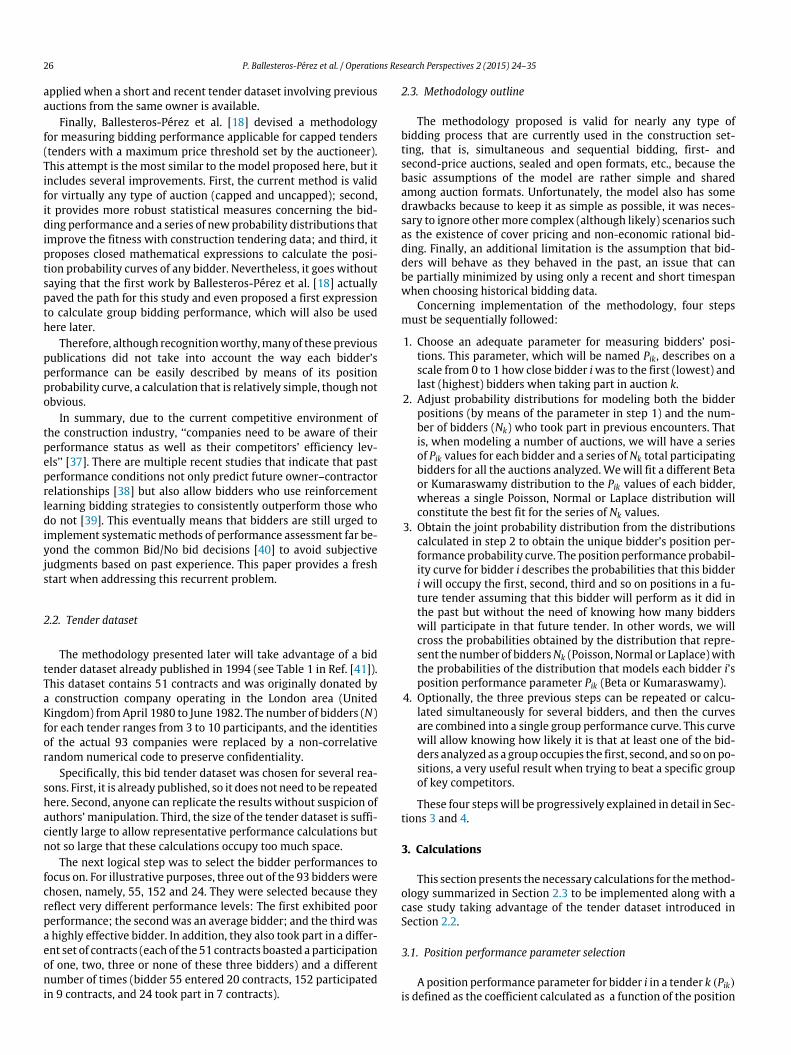
Table 5Position performance joint probability curves for bidders i = 1, 2 and 3.

ji J1 PDF J1 CDF J2 PDF J2 CDF J3 PDF J3 CDF

1 0.077 0.077 0.230 0.230 0.402 0.4022 0.127 0.204 0.169 0.399 0.316 0.7183 0.159 0.362 0.154 0.552 0.171 0.8894 0.181 0.544 0.145 0.697 0.075 0.9645 0.191 0.735 0.134 0.831 0.026 0.9906 0.164 0.899 0.106 0.936 0.007 0.9987 0.067 0.966 0.042 0.978 0.002 0.9998 0.023 0.988 0.014 0.993 0.000 1.0009 0.008 0.996 0.005 0.997 0.000 1.000

10 0.003 0.999 0.002 0.999 0.000 1.00011 0.001 0.999 0.001 1.000 0.000 1.000

Fig. 3. Position performance joint probability curves for bidders i = 1, 2 and 3.

so far. For instance, as displayed in Fig. 3, Bidder 3 is the toughercompetitor because it has higher chances of occupying the first po-sitions compared to Bidders 2 and 3. At the same time, Bidder 2 sta-tistically outperforms Bidder 1 in the first three positions (ji = 1, 2and 3). Hence, if a tendermanager had to focus on beating a specificcompetitor, it would be Bidder 3.

Furthermore, a third use can be made of this methodologybecause it allows aggregating several bidders’ probability curvesas a group to calculate the probability that one of them occupieda given position. This is a remarkable feature for a tender managerwhose concern is to beat several competitors at the same time andwill be implemented below.

4.2. Group of bidders’ position performance joint probability curve

A previous study, [18] proposed a way of calculating groupperformance curves for capped tenders based on the probabilitythat several independent random events took place. This approachis equally valid here with hardly any changes:

⌢J i PDF (x = ji) = 1 −

i=ni=1

(1 − Ri · Ji PDF) (11)

where:⌢J i PDF (·) is a discrete probability density function that denotesthe probability that one of the bidders (i = 1, . . . , n) occupiesthe position x = ji.Ri are the bidders’ participation ratios calculated at the bottomof Table 2, which represent how frequently each bidder partic-ipates in the set of tenders analyzed; therefore, 0 ≤ Ri ≤ 1.

Finally, Ji PDF are the bidder i’s position performance jointprobability density function for i = 1, . . . , n calculated accordingto Eq. (10).

32 P. Ballesteros-Pérez et al. / Operations Research Perspectives 2 (2015) 24–35

Table 6Group (bidders i = 1 + 2 + 3) position performance probability curve calculations.

Bidders’ participation ratios

i = 1 2 3Ri = 0.392 0.176 0.137

ji R1 ∗ J1 PDF R2 ∗ J2 PDF R3 ∗ J3 PDF PDF CDF1 − Π(1 − Ri ∗ Ji) 1 − Π(1 − Ri ∗ Ji)

1 0.030 0.041 0.055 0.121 0.1212 0.050 0.030 0.043 0.118 0.2393 0.062 0.027 0.023 0.109 0.3484 0.071 0.026 0.010 0.104 0.4525 0.075 0.024 0.004 0.100 0.5526 0.064 0.019 0.001 0.083 0.6357 0.026 0.007 0.000 0.034 0.6688 0.009 0.002 0.000 0.011 0.6809 0.003 0.001 0.000 0.004 0.684

10 0.001 0.000 0.000 0.001 0.68511 0.000 0.000 0.000 0.000 0.685

Fig. 4. Group (bidders i = 1 + 2 + 3) position performance probability curve.

Therefore, if Eq. (11) is applied to bidders i = 1, 2 and 3’sposition performance curves, Table 6 and Fig. 4 are easily obtained.

It is easy to note that the gray curve with thick line (obtainedby applying Eq. (11)) will only reach the 100% probability valuein the case that all the bidders from the tender dataset analyzedwere incorporated into the calculations (93 bidders for the tenderdataset presented in Section 2.2). Indeed, this is the reason forwhich these curves become flat when compared to Fig. 3.

Indeed, from Fig. 4, it is easy to determine that the probabilitiesthat one bidder out of bidders i = 1, 2 and 3 occupies thefirst position (when no one knows how many or which bidderswill participate) are approximately 12% and remain slightlydecreasingly at approximately the 10% probability value up to thesixth position. Of course, none of these probability values seem tobe too high to worry other competitors; however, this is due tothe fact that these three bidders do not have high participationratios, as shown at the top of Table 6. If any bidder knew for certainthat one or several of these bidders is going to enter a bid in aforthcoming tender, these curves could be recalculated assigninga 100% participation ratio value to those specific competitors, aswas considered in Fig. 3, and the group curve would raise theirprobabilities significantly, thus making the group of bidders 1, 2and 3muchmore competitive (for instance, bidder 1 alone reached40% probability values of occupying the first position when itsparticipation ratio was 100%, as Fig. 3 indicates).

With these last observations and calculations, every possibleapproach to study any bidder’s position performance has beencompleted, and therefore, the case study is also complete.

Fig. 5. Bidders i = 1’s actual and model position performance probability curvescomparison.

4.3. Validation

As stated in the Introduction, the main reason to calculate theposition performance curves by means of the method explainedso far instead of directly calculating the relative frequency curves,which would describe how often a bidder ends up being thefirst, second, and so on, was that in real-life situations, there isnot usually a sufficient number of previous encounters amongconstruction bidders for these probability values to be calculatedwith accuracy.

Particularly, in the tender database used in this analysis, the firstbidder (i = 1) was nearly the only onewith sufficient participation(in addition to the bidder who gathered the complete database,which has not been displayed) to draw up its probability curves.To be exact, the first bidder participated 20 times out of the total51, so if we represented its actual position performance densityand cumulative curves, the result compared to the ones obtainedin the model is depicted in Fig. 5.

Both couple of curves evidence quite similar trajectories,especially taking into account that the amount of data only allowedfor 5%-probability steps, i.e., 1/20. This fact qualitatively validatesthat the results were quite close to the reality, although a deeperanalysis might have been made if this bidder had participated inmanymore occasions. Nevertheless, froma 51-tender dataset, onlytwo bidders out of 93 companies had sufficient data to barelyrepresent their curves (the next most frequent bidder took partin 12 auctions), which means that in general, even with far biggerdatasets, a significant percentage of the participating bidders couldnot be analyzed directly but for the method proposed here.

P. Ballesteros-Pérez et al. / Operations Research Perspectives 2 (2015) 24–35 33

This is indeed the real advantage of the model and the evi-dence of the applicability in the construction industry: The pro-posed model allows for the analysis of the number of total partic-ipating bidders and the position performance of every bidder ona scale from 0 to 1, even when resorting to far shorter databases.Later, these results are aggregated into the single or group posi-tion probability curves, which are not expected to deviate muchfrom the actual (but unknown, due to data scarcity) position per-formance curves.

Unfortunately, short tender databases along with the unique-project nature are common features of the construction context.Therefore, the method proposed, although not free of limitations,constitutes an approximate but useful tool.

5. Discussion

Early bid tender models (e.g., [6–10]) took into account thebid/cost ratio, the probability of winning and a few other variablesunder the condition that the product quality does not vary withthe price [36]. This last condition does not usually hold in real-life situations [47], so the lowest bidder stops being identifiedwith the most advantageous tenderer [11]. With this in mind,the methodology proposed above allows anyone analyzing a setof tender processes to calculate the position probability curvesbased on those bidders potentially involved in future tendersassuming that they will perform in accordance with their previousperformance.

Specifically, by means of a four-step procedure, the bestposition performance parameter expression has been chosen forbidders, and subsequently, by gathering a series of these parametervalues for different bidders, the Kumaraswamy distribution hasbeen found to be a good candidate for modeling a single bidder’sposition performance when the number of participating bidders isknown.

However, through modeling the number of bidders in parallelby means of the Laplace distribution, the position performancecurve can be easily expressed irrespective of the number ofbidders, a convenient feature because, generally, the number ofparticipating bidders in future tenders is not knownbefore a tenderreaches its deadline in the Construction context.

Finally, the single bidder’s position performance curves can beanalyzed either independently or as a group, enhancing the appli-cability of the methodology because it is also quite common thatone company who enters a bidding process is forced somehow toeconomically outperform several key competitors simultaneously.Nonetheless, the methodology also has two mathematical minorlimitations. First, the Kumaraswamy distribution can be nearly (asa function of its two shape parameters αi and βi) but not totallysymmetrical, which means that in case a bidder i’s half number ofparameters equaled Pik and the other half equaled 1− Pik, the Betadistribution would always have a slightly lower p-value becausethe Beta distribution can actually be totally symmetrical as long asai = bi.

The second limitation is that both the Kumaraswamy and theBeta distribution require at least two previous non-equal Pik valuesto be fitted, that is, when a tender dataset comprises bidderswho only participated in one tender or when a bidder repeatsthe same position against the same number of competing bidders,it is advisable to resort to a simpler expression for which thesupports are [0, 1] in both axes (as in the Beta and Kumaraswamydistributions) instead of using Eq. (4), which is:

F (x) = F (x, γi) = xγi (12)

with γi = LN 0.5/LN Pik and Pik being the unique (repeated or not)value position performance coefficient obtained by bidder i in theone or several tenders k (Pik calculated according to Eq. (2)).

Furthermore, if a tender manager wanted to model a bidderfrom whom no previous encounters were available, it would bebetter to define its position performance curve parameters (eitherBeta’s or Kumaraswamy’s) as totally random, i.e., ai = bi = αi =

βi = 1.Finally, an additional pending issue that justified the selection

of the Kumaraswamy’s over the Beta distribution was that thelatter has less friendly cumulative and quantile distributionfunctions because they involve an Incomplete Beta function. Themajor finding of this paper, Eq. (10), made use of Kumaraswamy’sCDF, but it is obvious that the quantile function can also be usefulwhen, given a particular probability value y, it is recommendedto calculate how many participating bidders Nk with which aparticular bidder would be capable of ending first, second or inany specific position ji (Eq. (13)); or, on the contrary, with a givennumber of bidders Nk, the best position that bidder i could achieve(Eq. (14)).

Both questions stem from the same expression, which takesadvantage of Eq. (5):1 − (1 − y)1/β

1/α=

Nk − jiNk

.

The expression above leads to Eqs. (13) and (14) when eithervariable’s bidder i’s position (ji) or number of bidders (Nk) areworked out, respectively:

Nk = ji/1 −

1 − (1 − y)1/β

1/α(13)

ji = Nk

1 −

1 − (1 − y)1/β

1/α. (14)

6. Conclusions

The ‘‘lowest bidmethod’’ has beendominant in the constructionindustry for many years and that is why the majority of bid tenderforecasting models focused initially on the lowest bidder’s bids.However, multi-attribute auctions give out a score to each bid,which is eventually added up to the technical score, allowingthe auctioneer to determine the bidder that deserves to be theawardee. This paper focuses on analyzing the economic biddingperformance by means of studying the bid order in a series ofhomogeneous auctions in which the awarding criterion mightinclude more aspects in addition to the price. Obviously, if theonly awarding criterion is the price, bidders’ positions are notimportant except for the lowest bidder (first position); conversely,when other technical criteria are included to obtain the finalbidders’ ranking (such as inmulti-attribute auctions), knowing theprobabilities of occupying a given position as a consequence of theeconomic bid becomes more important.

The methodology proposed in this paper addresses theproblem of quantitatively defining what level of bidding positionperformance should be expected when a bidder takes part ina future auction, that is, determining the more likely positionsthat the bidder will occupy when competing against a known orunknown number of bidders in a construction auction. In addition,the auction format was stated as not relevant when applying themethodology discussed above because all construction auctionformats share the same variables the methodology makes use of,i.e., bidders’ identities and positions as well as total number ofparticipating bidders.

Additionally, the bidders’ position performance can be treatedindividually or as a group, allowing a tender manager to enrichthe analysis by calculating the probabilities that at least one bidderamong several reaches any position in a competitive tender.

On the other hand, the methodology proposed involves theuse of Kumaraswamy’s distribution, possibly for the first time,

34 P. Ballesteros-Pérez et al. / Operations Research Perspectives 2 (2015) 24–35

in construction management, as well as the Laplace distributionfor modeling the number of participating bidders. However, thislast distribution might not be the best alternative for other tenderdatabases in which the PDF describing the number of bidders wereconvex, being the other available non-parametric alternatives alsoanalyzed here (the Poisson or the Normal distribution).

This paper has proposed an entirely different way of measuringbidding competitiveness in construction tenders, the applicationsof which, although not entirely flawless, as stated in theDiscussions section, might go beyond the ones anticipated herewhen analyzing a single or a group of bidders’ performance.

In particular, the main limitations of this research are inherentto the model hypotheses because it necessarily assumes thatbidders will behave as they behaved in the past, whereas coverpricing and non-economic rational bidding are ignored. Thesethree assumptions limit the practical use of the model developedwhile actually opening a future topic of research: achieving amoreuseful practical tool for modeling bidding position performancethat is not dependent on these three previous assumptions.

Furthermore, there are other obvious shortcomings in the cur-rent experiment with regard to the case study database; theauthors have made use of an old database that did not use elec-tronic auctioning processes and from which multi-parameter bid-ding datawere certainly not available, thereby limiting the analysisto the study of the economic bid positions. Therefore, the authors’acknowledge that there is certainly a room for improvement, forinstance, in order to free future models from the limitations andhypotheses stated above, therefore, further research needs to bedone in this area.

Acknowledgment

This research study was funded in Chile by CONICYT under thePrograms Initiation into research 2013 (project number 11130666)and 2014 (project number 11140128).

References

[1] EC-Harris-LLP, BIS Research Paper No. 145. Supply Chain Analysis into theConstruction Industry. A Report for the Construction Industrial Strategy, 2013,p. 35–8.https://www.gov.uk/government/uploads/system/uploads/attachment_data/file/252026/bis-13-1168-supply-chain-analysis-into-the-construction-industry-report-for-the-construction-industrial-strategy.pdf.

[2] Ballesteros-Pérez P, González-Cruz MC, Pastor-Ferrando JP. Analysis ofconstruction projects by means of value curves. Int J Proj Manage 2010;28:719–31. http://dx.doi.org/10.1016/j.ijproman.2009.11.003.

[3] Benton WC, McHenry LF. Construction purchasing and supply chain manage-ment. McGraw-Hill; 2010. http://psbm.org/Ebooks/ConstructionSupply.pdf.

[4] Pim JC. Competitive tendering andbidding strategy. Natl Build 1974;55:541–5.[5] Skitmore M. Predicting the probability of winning sealed bid auctions: the

effect of outliers on bidding models. Constr Manag Econ 2004;22:101–9.[6] Friedman L. A competitive bidding strategy. Oper Res 1956;1:104–12.[7] Gates M. Bidding strategies and probabilities. J Constr Div Proc Am Soc Civ Eng

1967;93:75–107.[8] Wade RL, Harris RB. LOMARK: A bidding strategy. J Constr Div 1976;102:

197–211. http://cedb.asce.org/cgi/WWWdisplay.cgi?6528 [accessed August12, 2014].

[9] Carr RI. General bidding model. J Constr Div Proc Am Soc Civ Eng 1982;108:639–50.

[10] Skitmore M. The contract bidder homogeneity assumption: an empiricalanalysis. Constr Manag Econ 1991;9:403–29.

[11] Perng Y-H, Juan Y-K, Chien S-F. Exploring the bidding situa-tion for economically most advantageous tender projects us-ing a bidding game. J Constr Eng Manage 2006;132:1037–42.http://dx.doi.org/10.1061/(ASCE)0733-9364(2006)132:10(1037).

[12] Bergman MA, Lundberg S. Tender evaluation and supplier selectionmethods in public procurement. J Purch Supply Manag 2013;19:73–83.http://dx.doi.org/10.1016/j.pursup.2013.02.003.

[13] Yu W, Wang K-W, Wang M-T. Pricing strategy for bestvalue tender. J Constr Eng Manage 2013;139:675–84.http://dx.doi.org/10.1061/(ASCE)CO.1943-7862.0000635.

[14] Lo W, Yan MR. A system review of competitive bidding and qualification-based selection systems. In: C. 2007 conf.—constr. manag. econ. ’past, presentfutur., 2007. p. 131–41. http://www.scopus.com/inward/record.url?eid=2-s2.0-84877591303&partnerID=tZOtx3y1.

[15] Fuentes-Bargues JL, González-Cruz MC, González-Gaya C. La contrataciónpública de obras: situación actual y puntos de mejora. Inf Constr 2014; [inSpanish] in press. http://dx.doi.org/10.3989/ic.12.130.

[16] Ballesteros-Pérez P, González-Cruz MC, Cañavate-Grimal A. Mathematicalrelationships between scoring parameters in capped tendering. Int J ProjManage 2012;30:850–62. http://dx.doi.org/10.1016/j.ijproman.2012.01.008.

[17] Mahdavi A, Hastak M. Quantitative analysis of bidding strategies: A hybridagent based-system dynamics approach. In: Constr. res. congr. 2014 constr. aglob. netw.—proc. 2014 constr. res. congr. American Society of Civil Engineers(ASCE); 2014. p. 1129–38. http://dx.doi.org/10.1061/9780784413517.0116.

[18] Ballesteros-Pérez P, González-Cruz MC, Fernández-Diego M, Pellicer E. Esti-mating future bidding performance of competitor bidders in capped tenders. JCiv EngManag 2014;1–12. http://dx.doi.org/10.3846/13923730.2014.914096.

[19] Drew DS, Skitmore RM. Competitiveness in bidding: a con-sultant’s perspective. Constr Manag Econ 1992;10:227–47.http://dx.doi.org/10.1080/01446199200000020.

[20] Jin Z, Deng F, Li H, SkitmoreM. Practical framework formeasuring performanceof international construction firms. J Constr Eng Manage 2013;139:1154–67.http://dx.doi.org/10.1061/(ASCE)CO.1943-7862.0000718.

[21] Pellicer TM, Pellicer E, Eaton D. A macroeconomic regression analysis of theEuropean construction industry. Eng Constr Archit Manag 2009;16:573–97.http://dx.doi.org/10.1108/09699980911002584.

[22] Sohn T-H, Kim H-R, Jang H-S. An MDB business competency assessmentof Korean construction companies. KSCE J Civ Eng 2013;18:1314–21.http://dx.doi.org/10.1007/s12205-013-0478-7.

[23] Drew D.S., Skitmore M.. Analysing bidding performance; measuring theinfluence of contract size and type. In: CIB W-55/65. 1990. p. 129–39.

[24] Jap SD, Naik Pa. BidAnalyzer: a method for estimation and se-lection of dynamic bidding models. Mark Sci 2008;27:949–60.http://dx.doi.org/10.1287/mksc.1080.0363.

[25] Flanagan R, Norman G. An examination of the tendering pattern of individualbuilding contractors. Build Technol Manag 1982;25–8. April.

[26] Pastor-Ferrando JP, Aragonés-Beltrán P, Hospitaler-Pérez A, García-Melón M.An ANP- and AHP-based approach for weighting criteria in public works bid-ding. J Oper Res Soc 2010;61:905–16. http://dx.doi.org/10.1057/jors.2010.13.

[27] Yu I, Kim K, Jung Y, Chin S. Comparable performance measurementsystem for construction companies. J Manage Eng 2007;23:131–9.http://dx.doi.org/10.1061/(ASCE)0742-597X(2007)23:3(131).

[28] Ballesteros-Pérez P, Skitmore M, Das R, del Campo-Hitschfeld ML. Quickabnormal-bid-detection method for construction contract auctions. J ConstrEng Manage 2015; http://dx.doi.org/10.1061/(ASCE)CO.1943-7862.0000978.In press.

[29] Fuentes-Bargues JL, González-Gaya C. Determination of dispropor-tionate tenders in public procurement. J Invest Manag 2013;2:1–9.http://dx.doi.org/10.11648/j.jim.20130201.11.

[30] Ballesteros-Pérez P, González-Cruz MC, Cañavate-Grimal A, Pellicer E.Detecting abnormal and collusive bids in capped tendering. Autom Constr2013;31:215–29. http://dx.doi.org/10.1016/j.autcon.2012.11.036.

[31] Harper CM, Molenaar KR, Anderson S, Schexnayder C. Synthesis of per-formance measures for highway cost estimating. J Manage Eng 2014;30:04014005. http://dx.doi.org/10.1061/(ASCE)ME.1943-5479.0000244.

[32] Carr PG. Investigation of bid price competition measuredthrough prebid project estimates, actual bid prices, and num-ber of bidders. J Constr Eng Manage 2005;131:1165–72.http://dx.doi.org/10.1061/(ASCE)0733-9364(2005)131:11(1165).

[33] Schiereck D, Vogt J. Long-run M & A success of strategic bidders in theconstruction industry. Probl Perspect Manag 2013;11:46–67.

[34] McCabe B, Tran V, Ramani J. Construction prequalification using data envel-opment analysis. Can J Civ Eng 2005;32:183–93. http://www.ingentaconnect.com/content/nrc/cjce/2005/00000032/00000001/art00017 [accessed August13, 2014].

[35] El-Mashaleh MS. Decision to bid or not to bid: a data envelopment analysisapproach. Can J Civ Eng 2010;37:37–44. http://dx.doi.org/10.1139/L09-119.

[36] Wang KW, Der Yu W, Wang MT. Revenue/cost Analysis Model for bid-der’s competitive bidding strategy planning. J Chin Inst Civ HydraulEng 2014;26:81–94. http://www.scopus.com/inward/record.url?eid=2-s2.0-84904458977&partnerID=tZOtx3y1.

[37] Horta IM, Camanho AS. Competitive positioning and performance assess-ment in the construction industry. Expert Syst Appl 2014;41:974–83.http://dx.doi.org/10.1016/j.eswa.2013.06.064.

[38] Abdallah AAN, Darayseh M, Waples E. Incomplete contract, agency theoryand ethical performance: A synthesis of the factors affecting owners’ andcontractors’ performance in the bidding construction process. J Gen Manag2013;38:39–56. http://www.scopus.com/inward/record.url?eid=2-s2.0-84888404741&partnerID=tZOtx3y1.

[39] Kozan B, Zlatar I, Paravan D, Gubina AF. The advanced bidding strategy forpower generators based on reinforcement learning. Energy Sources Part B2014;9:79–86. http://dx.doi.org/10.1080/15567241003792358.

[40] Polat G, Bingol BN, Uysalol E. Modeling Bid/No bid decision usingadaptive neuro fuzzy inference system (ANFIS): a case study. In: Con-str. res. congr. 2014 constr. a glob. netw.—proc. 2014 constr. res.congr. American Society of Civil Engineers (ASCE); 2014. p. 1083–92.http://dx.doi.org/10.1061/9780784413517.0111.

[41] Skitmore M, Pemberton J. A multivariate approach to construction contractbidding mark-up strategies. J Oper Res Soc 1994;45:1263–72.

P. Ballesteros-Pérez et al. / Operations Research Perspectives 2 (2015) 24–35 35

[42] Ballesteros-Pérez P, González-Cruz MC, Cañavate-Grimal A. On competitivebidding: scoring and position probability graphs. Int J Proj Manage 2013;31:434–48. http://dx.doi.org/10.1016/j.ijproman.2012.09.012.

[43] Ballesteros-Pérez P, González-Cruz MC, Pastor-Ferrando JP, Fernández-DiegoM. The iso-score curve graph. A new tool for competitive bidding. AutomConstr 2012;22:481–90. http://dx.doi.org/10.1016/j.autcon.2011.11.007.

[44] Jones MC. Kumaraswamy’s distribution: A beta-type distributionwith some tractability advantages. Stat Methodol 2009;6:70–81.http://dx.doi.org/10.1016/j.stamet.2008.04.001.

[45] Kumaraswamy P. A generalized probability density function fordouble-bounded random processes. J Hydrol 1980;46:79–88.http://dx.doi.org/10.1016/0022-1694(80)90036-0.

[46] Engelbrecht-Wiggans R. A model for the distribution of the number of biddersin an auction. In: Cowles Found. discuss. pap. 495. 1978. pp. 1–13.

[47] Laryea S, Hughes W. Risk and price in the bidding process of contractors. JConstr EngManage 2011;137:248–58. http://cedb.asce.org/cgi/WWWdisplay.cgi?278030 [accessed September 01, 2014].