EXPERIMENT-1 Aim-Introduction to MATLAB Theory- Introduction to MATLAB
Upload
khangminh22Category
view
2download
0
glmlabUsing MATLAB for analysinggeneralised linear models
Peter K. Dunn

i

ii
glmlabUsing MATLAB for analysinggeneralised linear models
Current version: 2.5
Peter K. DunnDepartment of Mathematics and ComputingUniversity of Southern QueenslandToowoomba, Australia
Printed: April 26, 2000
This manual has been produced using LATEXand MATLAB, converted to HTML using hyperlatex, andis c
�1997–2000 Peter K. Dunn.

iii
Table of Contents
Acknowledgements . . . . . . . . . . . . . . . . . . . . . . . . . . . . . . . . . . . . . . viiiA Note on What You Read . . . . . . . . . . . . . . . . . . . . . . . . . . . . . . . . . . viiiContact Information . . . . . . . . . . . . . . . . . . . . . . . . . . . . . . . . . . . . . . viii
1 Introduction 11.1 Why glmlab? . . . . . . . . . . . . . . . . . . . . . . . . . . . . . . . . . . . . . 11.2 What can glmlab do? . . . . . . . . . . . . . . . . . . . . . . . . . . . . . . . . . 11.3 Installing glmlab . . . . . . . . . . . . . . . . . . . . . . . . . . . . . . . . . . . 2
1.3.1 The PC Version of MATLAB . . . . . . . . . . . . . . . . . . . . . . . . . . 21.3.2 The UNIX and LINUX Versions of MATLAB . . . . . . . . . . . . . . . . . . 3
1.4 Directory Structure . . . . . . . . . . . . . . . . . . . . . . . . . . . . . . . . . . . 3
2 Starting with MATLAB 42.1 Basic Use of MATLAB . . . . . . . . . . . . . . . . . . . . . . . . . . . . . . . . . . 42.2 Obtaining Help from MATLAB . . . . . . . . . . . . . . . . . . . . . . . . . . . . . 62.3 Using Data Files . . . . . . . . . . . . . . . . . . . . . . . . . . . . . . . . . . . . 72.4 Using MATLAB for Plotting . . . . . . . . . . . . . . . . . . . . . . . . . . . . . . . 92.5 Other Miscellaneous MATLAB Commands . . . . . . . . . . . . . . . . . . . . . . . 10
Some Examples . . . . . . . . . . . . . . . . . . . . . . . . . . . . . . . . . . . . . 11
3 glmlab Reference 123.1 The Main Window Items . . . . . . . . . . . . . . . . . . . . . . . . . . . . . . . . 12
3.1.1 The File Menu . . . . . . . . . . . . . . . . . . . . . . . . . . . . . . . . . 123.1.2 The Distributions Menu . . . . . . . . . . . . . . . . . . . . . . . . . . . . 143.1.3 The Link Menu . . . . . . . . . . . . . . . . . . . . . . . . . . . . . . . . . 143.1.4 The Scale Parameter Menu . . . . . . . . . . . . . . . . . . . . . . . . . . . 143.1.5 The Residuals Type Menu . . . . . . . . . . . . . . . . . . . . . . . . . . . 143.1.6 The Options Menu . . . . . . . . . . . . . . . . . . . . . . . . . . . . . . . 143.1.7 The Plots Menu . . . . . . . . . . . . . . . . . . . . . . . . . . . . . . . . . 153.1.8 The Help Menu . . . . . . . . . . . . . . . . . . . . . . . . . . . . . . . . . 16
3.2 The Main Window Edit Areas . . . . . . . . . . . . . . . . . . . . . . . . . . . . . 173.2.1 The Response Area . . . . . . . . . . . . . . . . . . . . . . . . . . . . . . . 173.2.2 The Covariates Area . . . . . . . . . . . . . . . . . . . . . . . . . . . . . . 183.2.3 The Prior Weights Area . . . . . . . . . . . . . . . . . . . . . . . . . . . . 183.2.4 The Offset Area . . . . . . . . . . . . . . . . . . . . . . . . . . . . . . . . . 18
3.3 The Main Window Buttons . . . . . . . . . . . . . . . . . . . . . . . . . . . . . . . 183.3.1 QUIT . . . . . . . . . . . . . . . . . . . . . . . . . . . . . . . . . . . . . . 18
iv
TABLE OF CONTENTS v
3.3.2 FIT SPECIFIED MODEL . . . . . . . . . . . . . . . . . . . . . . . . . . . 183.3.3 NEW MODEL . . . . . . . . . . . . . . . . . . . . . . . . . . . . . . . . . 19
3.4 Extra Commands . . . . . . . . . . . . . . . . . . . . . . . . . . . . . . . . . . . . 193.4.1 fac . . . . . . . . . . . . . . . . . . . . . . . . . . . . . . . . . . . . . . . 193.4.2 makefac . . . . . . . . . . . . . . . . . . . . . . . . . . . . . . . . . . . . 193.4.3 The @ Character . . . . . . . . . . . . . . . . . . . . . . . . . . . . . . . . 19
3.5 Returned Variables . . . . . . . . . . . . . . . . . . . . . . . . . . . . . . . . . . . 19
4 Examples Using glmlab 214.1 Example: Multiple Regression . . . . . . . . . . . . . . . . . . . . . . . . . . . . . 214.2 Example: Log-Linear Models . . . . . . . . . . . . . . . . . . . . . . . . . . . . . . 26
5 Advanced Topics and Examples 305.1 Offsets . . . . . . . . . . . . . . . . . . . . . . . . . . . . . . . . . . . . . . . . . . 305.2 Default Settings for Distributions . . . . . . . . . . . . . . . . . . . . . . . . . . . . 305.3 Changing the Scale Parameter . . . . . . . . . . . . . . . . . . . . . . . . . . . . . 305.4 Example: A Generalised Linear Model . . . . . . . . . . . . . . . . . . . . . . . . . 325.5 Example: Binomial Distributions . . . . . . . . . . . . . . . . . . . . . . . . . . . . 345.6 User Defined Links and Distributions . . . . . . . . . . . . . . . . . . . . . . . . . 355.7 Example: User Defined Distributions . . . . . . . . . . . . . . . . . . . . . . . . . . 355.8 The Default Data Directory . . . . . . . . . . . . . . . . . . . . . . . . . . . . . . . 365.9 npplot . . . . . . . . . . . . . . . . . . . . . . . . . . . . . . . . . . . . . . . . . 375.10 Changing the Fitting Parameters . . . . . . . . . . . . . . . . . . . . . . . . . . . . 37
References 38
Index 38

List of Figures
1.1 The MATLAB Windows Path . . . . . . . . . . . . . . . . . . . . . . . . . . . . . . 21.2 The MATLAB UNIX Path in tc shell . . . . . . . . . . . . . . . . . . . . . . . . 31.3 The Structure of glmlab . . . . . . . . . . . . . . . . . . . . . . . . . . . . . . . . 3
2.1 Graph of y � exp���
x2 � . . . . . . . . . . . . . . . . . . . . . . . . . . . . . . . . . . 11
3.1 A Quick Tour of the glmlab Screen . . . . . . . . . . . . . . . . . . . . . . . . . . 133.2 A Quick Tour of the Drop-Down Menus . . . . . . . . . . . . . . . . . . . . . . . . 13
4.1 The Initial glmlab Screen . . . . . . . . . . . . . . . . . . . . . . . . . . . . . . . 224.2 Variables Being Entered for Chemical Data . . . . . . . . . . . . . . . . . . . . . . 244.3 Entering Data Using the fac Command . . . . . . . . . . . . . . . . . . . . . . . . 244.4 Selecting the Poisson Distribution . . . . . . . . . . . . . . . . . . . . . . . . . . . 274.5 Response and Prior Weights Only Entered . . . . . . . . . . . . . . . . . . . . . . . 274.6 Including an Interaction Term . . . . . . . . . . . . . . . . . . . . . . . . . . . . . 29
5.1 Entering a Fixed Value for the Scale Parameter . . . . . . . . . . . . . . . . . . . . 335.2 Variables Entered for Example 5.4 . . . . . . . . . . . . . . . . . . . . . . . . . . . 335.3 Variables Entered for the Beetle Mortality Example . . . . . . . . . . . . . . . . . . 355.4 The Fitting Parameters Window . . . . . . . . . . . . . . . . . . . . . . . . . . . . 37
vi
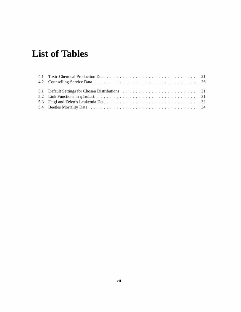
List of Tables
4.1 Toxic Chemical Production Data . . . . . . . . . . . . . . . . . . . . . . . . . . . . 214.2 Counselling Service Data . . . . . . . . . . . . . . . . . . . . . . . . . . . . . . . . 26
5.1 Default Settings for Chosen Distributions . . . . . . . . . . . . . . . . . . . . . . . 315.2 Link Functions in glmlab . . . . . . . . . . . . . . . . . . . . . . . . . . . . . . . 315.3 Feigl and Zelen’s Leukemia Data . . . . . . . . . . . . . . . . . . . . . . . . . . . . 325.4 Beetles Mortality Data . . . . . . . . . . . . . . . . . . . . . . . . . . . . . . . . . 34
vii

LIST OF TABLES viii
Acknowledgements
The author wishes to thank Mr Henry Eastment and Mr Michael Simpson for their help and advicewith glmlab, and for enduring the many frustrating errors of the earlier versions. Thanks also toJim Albert and especially G. Janacek for their encouragement in trying early versions of glmlab.Thanks also to Jean-Marc Fromentin for help with later problems.
A Note on What You Read
Some small differences may exist between the figures that appear in this document and the figures thatappear on your computer screen. Most of the figures that appear in this document are the figures asthey appear in the UNIX or LINUX versions. Windows and Macintosh versions will produce figuresthat are similar, but different.
glmlab is often updated in small ways. Some of the most recent changes may not appear in thefigures and output that is shown in this document (especially where dates are given).
This document was produced using LATEX and TEX, with the pictures produced (obviously) usingMATLAB.
Contact Information
There is no charge for using glmlab. However, if you find it useful, it would be greatly appreciatedif you could contact the author and let him know how you are using glmlab, by emailing him [email protected], or (preferred) writing to:
Peter DunnFaculty of SciencesUSQToowoomba Q 4350AUSTRALIA
You may also find it useful to visit the glmlab Home Page on the web at http://www.sci.usq.edu.au/staff/dunn/glmlab/glmlab.html.

Chapter 1
Introduction
1.1 Why glmlab?
glmlab was first written in 1995 to emulate some of the features of GLIM (Aitken et al. [1], Franciset al. [6]), industry standard software for analysing generalised linear models. However, GLIM isan expensive program to purchase (even student editions). Since MATLAB is inexpensive in studenteditions (especially considering its capabilities) and is a widely used numerical computation package,MATLAB was considered an ideal platform in which to perform the analyses performed in GLIM.glmlab does not attempt to replace packages such as GLIM and S-PLUS (Statistical Sciences [9]),but rather to bring the world of generalised linear models to the MATLAB environment.
glmlab uses a graphical user interface, which means very few additional commands need to belearnt to use glmlab. This manual discusses some of the basic skills needed to use glmlab. Whileit assumes some knowledge of MATLAB, there is a introduction to MATLAB in Chapter 2
1.2 What can glmlab do?
MATLAB is a powerful computational tool that can be programmed to perform practically any numeri-cal task. MATLAB has some basic statistical procedures built-in (for example, hist, mean, medianand std). More statistical procedures are available—at extra cost—in the Statistics Toolbox. glm-lab extends MATLAB’s statistical capabilities without needing the Statistics Toolbox, allowing theuser to perform tasks such as:
� simple linear regression;� multiple regression;� weighted regression;� log-linear models;� logistic regression;� other generalised linear modelling techniques; and� residual plotting.
glmlab also allows the user to save models between sessions, and returns a number of variablesto the workspace for further analysis (see Section 3.5).
1

CHAPTER 1. INTRODUCTION 2
matlabpath([...’C:
�MATLAB
�toolbox
�local’,...
’;C:�MATLAB
�toolbox
�matlab
�datafun’,...
’;C:�MATLAB
�toolbox
�matlab
�elfun’,...
......
...’;C:
�MATLAB
�toolbox
�local’,...
’;C:�glmlab’,... ��� A new line to be included
’;C:�glmlab
�fit’,... ��� A new line to be included
’;C:�glmlab
�fit
�link’,... ��� A new line to be included
’;C:�glmlab
�fit
�dist’,... ��� A new line to be included
’;C:�glmlab
�misc’,... ��� A new line to be included
’;C:�glmlab
�plotting’,... ��� A new line to be included
’;C:�glmlab
�data’,... ��� A new line to be included
’;C:�glmlab
�glmhelp’,... ��� A new line to be included
’;C:�glmlab
�glmlog’,... ��� A new line to be included
]);
Figure 1.1: The MATLAB Windows Path
1.3 Installing glmlab
glmlab is available from the MathWorks user contributed site at http://wwww.mathworks.com/statsv5.html as glmlab.zip (best for Windows or Macintosh users) or glmlab.tar(best for UNIX users).
When installing glmlab, you will need to have write access to the glmlab/glmlog direc-tory/folder so that it can create a file of the fitting parameters and to place the log file. For this reason,it is suggested that glmlab be installed in your own directories. (This will make more sense afterreading the rest of this section.)
Please consult your MATLAB documentation to help with setting the appropriate MATLAB path.The steps outlined below can change and are sometimes platform dependent.
1.3.1 The PC Version of MATLAB
If you have the file glmlab.zip, you will need to “unzip” the file using a program such as PKunZipor WinZip.
After loading glmlab onto the computer’s hard disk, MATLAB must be told where to find theglmlab files. There are two ways to do this: one is to use the PathTool that comes with MATLAB,by typing pathtool at the MATLAB prompt. The second method is to edit the file matlabrc.m(generally found in the matlab directory). Load this file using a text editor (such as notepad oredit, or even a word processor) and find the section that begins with
matlabpath([...This section must be edited to include the glmlab directories. Use the editor to include some extralines so that it ends up looking similar to Figure 1.1 (many lines have been omitted).
Type help glmlab at the MATLAB prompt next time MATLAB is started. If the messageglmlab.m not found appears on the screen, then the installation did not work and will needto be repeated.
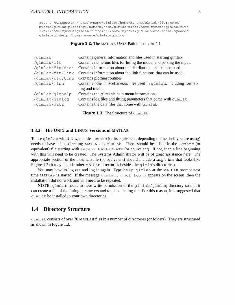
CHAPTER 1. INTRODUCTION 3
setenv MATLABPATH /home/myname/glmlab:/home/myname/glmlab/fit:/home/myname/glmlab/plotting:/home/myname/glmlab/misc:/home/myname/glmlab/fit/link:/home/myname/glmlab/fit/dist:/home/myname/glmlab/data:/home/myname/glmlab/glmhelp:/home/myname/glmlab/glmlog
Figure 1.2: The MATLAB UNIX Path in tc shell
/glmlab Contains general information and files used in starting glmlab./glmlab/fit Contains numerous files for fitting the model and parsing the input./glmlab/fit/dist Contains information about the distributions that can be used./glmlab/fit/link Contains information about the link functions that can be used./glmlab/plotting Contains plotting routines./glmlab/misc Contains other miscellaneous files used in glmlab, including format-
ting and tricks./glmlab/glmhelp Contains the glmlab help menu information./glmlab/glmlog Contains log files and fitting parameters that come with glmlab./glmlab/data Contains the data files that come with glmlab.
Figure 1.3: The Structure of glmlab
1.3.2 The UNIX and LINUX Versions of MATLAB
To use glmlabwith UNIX, the file .cshrc (or its equivalent, depending on the shell you are using)needs to have a line directing MATLAB to glmlab. There should be a line in the .cshrc (orequivalent) file starting with setenv MATLABPATH (or equivalent). If not, then a line beginningwith this will need to be created. The Systems Administrator will be of great assistance here. Theappropriate section of the .cshrc file (or equivalent) should include a single line that looks likeFigure 1.2 (it may include other MATLAB directories besides the glmlab directories).
You may have to log out and log in again. Type help glmlab at the MATLAB prompt nexttime MATLAB is started. If the message glmlab.m not found appears on the screen, then theinstallation did not work and will need to be repeated.
NOTE: glmlab needs to have write permission to the glmlab/glmlog directory so that itcan create a file of the fitting parameters and to place the log file. For this reason, it is suggested thatglmlab be installed in your own directories.
1.4 Directory Structure
glmlab consists of over 70 MATLAB files in a number of directories (or folders). They are structuredas shown in Figure 1.3.

Chapter 2
Starting with MATLAB
This section discusses, very briefly, how to start using MATLAB. Only details important for usingglmlab are discussed. A more thorough introduction is given in http://www.math.utah.edu/lab/ms/matlab/matlab.html. The MATLAB manual will also prove useful.
2.1 Basic Use of MATLAB
MATLAB is designed to work easily with matrices and vectors, and a number of methods exist todeclare matrices and vectors. For example, an entire matrix can be entered on one line with rowsseparated by semicolons (;):
>> A = [ 1 3 2 ; -1 0 9 ]A =
1 3 2-1 0 9
The matrix can also be typed in row by row:
>> A = [ 1 3 2-1 0 9]
A =1 3 2
-1 0 9
Notice that the spacing used has no effect. The transpose of a matrix can be found using the quotesymbol (’):
>> B = [0 3 ;3 4;6 6];>> B’ans =
0 3 63 4 6
The semicolon (;) at the end of a line stops MATLAB from displaying the answer on the screen. Basicmatrix operations can be performed:
>> A + B??? Error using ==> +Matrix dimensions must agree.
4

CHAPTER 2. STARTING WITH MATLAB 5
>> A + B’ans =
1 6 82 4 15
>> A - B’ans =
1 0 -4-4 -4 3
>> A * Bans =
21 2754 51
>> inv( A * B )ans =
-0.1318 0.06980.1395 -0.0543
There are other operations in MATLAB apart from the standard operations. Preceding an operationwith a period (.) causes the operation to be applied on an element by element basis. For example,consider the following commands:
>> C = [0 -3 4; 5 -4 3]C =
0 -3 45 -4 3
>> D = [1 1 9; -3 0 1]D =
1 1 9-3 0 1
>> C * D??? Error using ==> *Inner matrix dimensions must agree.
>> C .* Dans =
0 -3 36-15 0 3
Here’s another example of MATLAB’s element by element procedure:
>> E = [1:4]E =
1 2 3 4
>> E * E??? Error using ==> *Inner matrix dimensions must agree.
>> E ˆ2 %Eˆ2 is the same as E*E??? Error using ==> ˆMatrix must be square.
>> E .ˆ 2ans =
1 4 9 16
CHAPTER 2. STARTING WITH MATLAB 6
As demonstrated above, comments can be included in MATLAB with the % character. MATLAB
ignores any characters after this symbol. It is good practice in any programming to include commentsto explain details that are not immediately obvious.
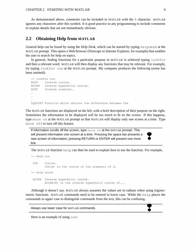
2.2 Obtaining Help from MATLAB
General help can be found by using the Help Desk, which can be started by typing helpdesk at theMATLAB prompt. This opens a Web browser (Netscape or Internet Explorer, for example) that enablesthe user to search for help on topics.
In general, finding functions for a particular purpose in MATLAB is achieved typing lookforand then a relevant word. MATLAB will then display any functions that may be relevant. For example,try typing lookfor cos at the MATLAB prompt. My computer produces the following (some hasbeen omitted):
>> lookfor cosACOS Inverse cosine.ACOSH Inverse hyperbolic cosine.ACSC Inverse cosecant....LQGCOST Function which returns the difference between the
The MATLAB functions are displayed on the left, with a brief description of their purpose on the right.Sometimes the information to be displayed will be too much to fit on the screen. If this happens,type more on at the MATLAB prompt so that MATLAB will display only one screen at a time. Typemore off to turn off this feature.
If information scrolls off the screen, type more on at the MATLAB prompt. Thiswill present information one screen at a time. Pressing the space bar presents anew screen of information; pressing RETURN or ENTER will present one moreline.
❢
The MATLAB function help can then be used to explain how to use the function. For example,
>> help cos
COS Cosine.COS(X) is the cosine of the elements of X.
>> help acosh
ACOSH Inverse hyperbolic cosine.ACOSH(X) is the inverse hyperbolic cosine of...
Although it doesn’t say, MATLAB always assumes the values are in radians when using trigono-metric functions. MATLAB commands need to be entered in lower case. While the help places thecommands in upper case to distinguish commands from the text, this can be confusing.
Always use lower case for MATLAB commands. ❢Here is an example of using cos:
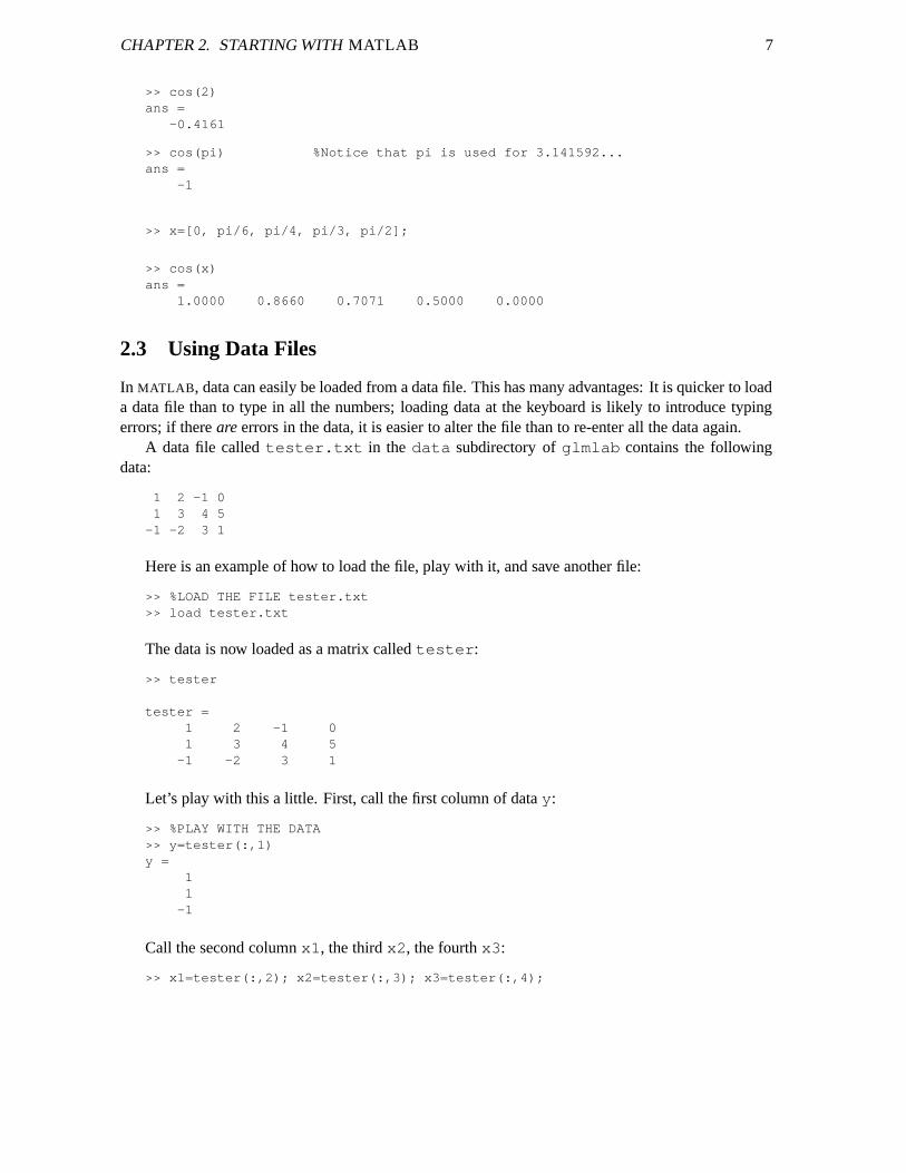
CHAPTER 2. STARTING WITH MATLAB 7
>> cos(2)ans =
-0.4161
>> cos(pi) %Notice that pi is used for 3.141592...ans =
-1
>> x=[0, pi/6, pi/4, pi/3, pi/2];
>> cos(x)ans =
1.0000 0.8660 0.7071 0.5000 0.0000
2.3 Using Data Files
In MATLAB, data can easily be loaded from a data file. This has many advantages: It is quicker to loada data file than to type in all the numbers; loading data at the keyboard is likely to introduce typingerrors; if there are errors in the data, it is easier to alter the file than to re-enter all the data again.
A data file called tester.txt in the data subdirectory of glmlab contains the followingdata:
1 2 -1 01 3 4 5
-1 -2 3 1
Here is an example of how to load the file, play with it, and save another file:
>> %LOAD THE FILE tester.txt>> load tester.txt
The data is now loaded as a matrix called tester:
>> tester
tester =1 2 -1 01 3 4 5
-1 -2 3 1
Let’s play with this a little. First, call the first column of data y:
>> %PLAY WITH THE DATA>> y=tester(:,1)y =
11
-1
Call the second column x1, the third x2, the fourth x3:
>> x1=tester(:,2); x2=tester(:,3); x3=tester(:,4);
CHAPTER 2. STARTING WITH MATLAB 8
Many commands can be placed on one line, separated by a semicolon or a comma. Notice, also,how to access particular columns of a matrix using a colon. Rows can be accessed in a similar way;r=tester(1,:)would place the first row of tester into row vector r.
In MATLAB, it is standard to define variables as column vectors. This standard isadopted by glmlab. ❢We can now manipulate the vectors:
>> x = x1 + x2 - 3 * x3x =
1-8-2
To save y and x in the file prac.txt, proceed as follows:
>> save prac.txt y x -ascii
That is,
save <filename>.<extension> <variables> -ascii
where the -ascii is so that humans can read it. However, the best way to save the file is to usesave <filename> <variables>:
>> save prac2 y x
This creates a file called prac2.mat which MATLAB can use, but humans can’t understand.To the load the file prac2.mat, simply type load prac2. This will automatically create twovariables (called x and y) without you having to declare them explicitly.
A file called loadme.mat should be in the glmlab data folder. First, clear all the currentvariables (using clear), and then load this file:
>> clear all>> load loadme
By typing who at the MATLAB prompt, the variables that have been loaded can be seen (try typingwhos also):
>> who
Your variables are:
x y z
Have a look at the variables (especially the variable called x) by typing variable names at the MATLAB
prompt.
When saving data, the best method is to use the syntax:save <filename> <variables> ❢
CHAPTER 2. STARTING WITH MATLAB 9
2.4 Using MATLAB for Plotting
MATLAB has many features to produce high quality plots. This section in no way explains all theplotting capabilities of MATLAB, or discusses all the ways in which things can be changed. Hopefullyit will supply you with enough information to be able to create plots that are near enough to what youwant.
The basic plotting command is plot. If you have defined two vectors (of the same length) namedx and y, then plot(x,y) will generate a plot of y versus x. A word of warning: By default,MATLAB joins the points with straight lines in the order in which they are given. To plot the points inother ways, use the following commands:
� plot(x,y,’+’)will use only plus signs at the points;� plot(x,y,’x’)will use only crosses at the points;� plot(x,y,’.’)will use only dots at the points;
For both lines and points, try these:
� plot(x,y,’+-’)will indicate the points with a plus sign, and join the points with straightunbroken lines.
� plot(x,y,’o--’)will indicate the points with a circle sign, and join the points with dashedlines.
A full list of the available type of points and lines is available by typing help plot first at theMATLAB prompt. (You may need to type more on at the prompt to see all the information.)
The plots should be annotated with labels on the x-axis, the y-axis and with a title. To place alabel on the x-axis, use xlabel; to place a label on the y-axis, use ylabel; and to place a title, usetitle.
Remember to always give pictures meaningful titles and axis labels. ❢Let’s have a look at using some of this information. First, define some vectors to manipulate:
>> x=[1:10]’; %The numbers 1, 2, ... 10>> y=randn(10,1); %10 by 1 vector of normally>> plot(x,y);
This gives a plot joining the points with lines, but crosses would be better:
>> plot(x,y,’x’);
The plot and the axes should be labelled:
>> xlabel(’x-values’);>> ylabel(’y-values’);>> title(’A plot of y versus x’);

CHAPTER 2. STARTING WITH MATLAB 10
The following functions may be useful also:
� axis: For example, axis([0 10 0 5]) sets the axes such that the x-axis ranges from 0 to10, and the y-axis ranges from 0 to 5.
� propedit: The property editor allows the user to make many changes to plots. Type propeditat the MATLAB prompt, and then click on the Figure to be edited. Change some of the settingsto see what happens.
To print the plots that are produced on the screen, the print command can be used, and usuallythe Print option from the File menu of the Figure works also. In some cases, it may be best to save thepicture to a file, and then print the file. The print command in still used in this case, but in a differentform. See the help for print for more information. (You may need to use more on.) Accordingto the help for print, the command print -depsonwill print the current picture on an Epson orEpson compatible 9- or 24-pin printer. Also, print -depson lookatme.prt should producea file called lookatme.prt that can be sent to an Epson printer. Type help print to see whatother types of printers that MATLAB supports (like LaserJets, BubbleJets and colour printers).
2.5 Other Miscellaneous MATLAB Commands
In this section, some other useful MATLAB commands are discussed. For a full description, see theMATLAB help for the function.
� sort: As the name suggests, sort sorts the data in ascending order. -sort(-x) sorts thedata in x in descending order.
� diary: Typing diary mine.txt at the MATLAB prompt creates a file called mine.txtcontaining all the information printed in the MATLAB command window from the time thecommand is entered. To turn off this feature, type diary off. (This can be useful whensubmitting assignments to show what was happened at the computer.)
� ones and zeros: These commands create vectors of ones and zeros of given size.� eye: This command create an identity matrix of a given size, usually called I.� size: This command returns the number of rows and the number of columns of a given matrix.� ans: Issuing this command at the MATLAB prompt recalls the last answer that wasn’t assigned
to another variable name.� ...: If the command line won’t fit on one line, end the line with three dots. This tells MATLAB
that the line that follows is a continuation of the previous line. For example, a large vector canbe defined like this:
>> HPrices=[150000, 200000, 125000, 350000, 89000, 110000, ...110000, 150000, 120000, 100900, 93500, 97000, ...88000, 118500, 123300, 165000, 95000]’;
When defining a long vector, it can be very useful to use the line continuationfacility by ending the lines with the characters .... ❢
CHAPTER 2. STARTING WITH MATLAB 11
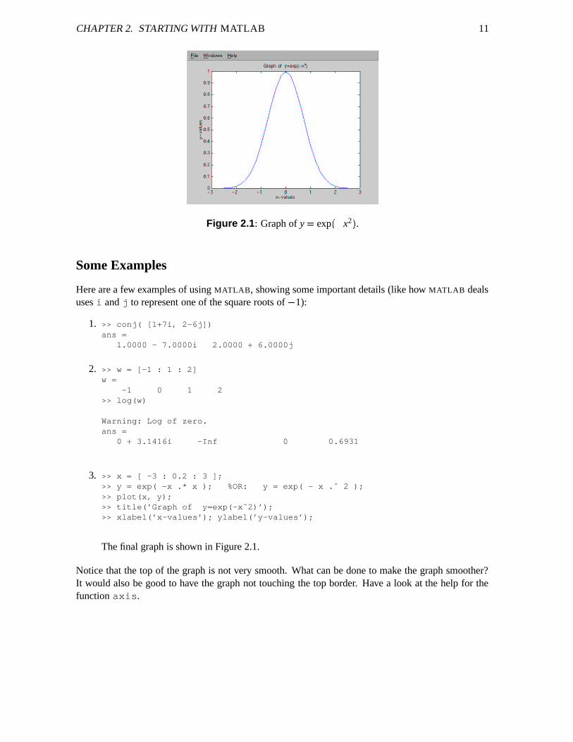
Figure 2.1: Graph of y � exp���
x2 � .
Some Examples
Here are a few examples of using MATLAB, showing some important details (like how MATLAB dealsuses i and j to represent one of the square roots of
�1):
1. >> conj( [1+7i, 2-6j])ans =
1.0000 - 7.0000i 2.0000 + 6.0000j
2. >> w = [-1 : 1 : 2]w =
-1 0 1 2>> log(w)
Warning: Log of zero.ans =
0 + 3.1416i -Inf 0 0.6931
3. >> x = [ -3 : 0.2 : 3 ];>> y = exp( -x .* x ); %OR: y = exp( - x .ˆ 2 );>> plot(x, y);>> title(’Graph of y=exp(-xˆ2)’);>> xlabel(’x-values’); ylabel(’y-values’);
The final graph is shown in Figure 2.1.
Notice that the top of the graph is not very smooth. What can be done to make the graph smoother?It would also be good to have the graph not touching the top border. Have a look at the help for thefunction axis.

Chapter 3
glmlab Reference
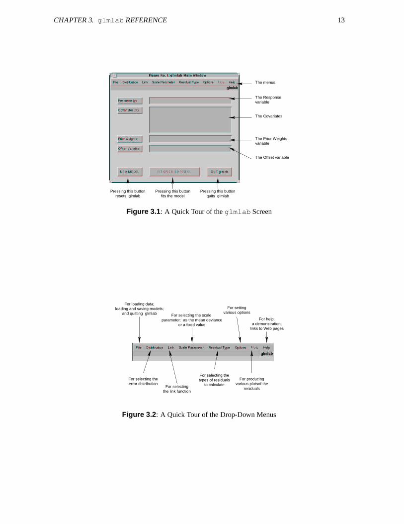
This section explains briefly most of the details of glmlab, including all of the main menu items.Figure 3.1 shows the main glmlab window.
3.1 The Main Window Items
There are eight drop-down menus on the main glmlab screen. For a quick explanation, see Fig-ure 3.2.
3.1.1 The File Menu
3.1.1.1 LOAD Data File
Allows the user to load a data file for use in glmlab, using a graphical interface. A dialog box isissued confirming that the file has loaded correctly.
The dialog box initially defaults to the glmlab data directory, but the default directory can bealtered by moving the dummydta.mfile to the required default folder/directory. See also Section 5.8.
3.1.1.2 Load glmlab Model
Loads a previously saved glmlabmodel, restoring details such as the error distribution, link function,scale parameter, residual type and variables entered.
3.1.1.3 Save glmlab Model
Saves a glmlab model, saving details such as the error distribution, link function, scale parameter,residual type and variables entered. A dialog box defaults to saving in the glmlog folder/directory,but this can be changed by moving the file dummylog.m to the desired directory.
3.1.1.4 QUIT glmlab
Quits glmlab and loses all information. The DETAILS.mfile will retain its information until glmlabis started again. This option is the same as pressing the QUIT button.
12
CHAPTER 3. glmlab REFERENCE 13
The menus
variable
The Covariates
The Prior Weightsvariable
The Offset variable
Pressing this buttonquits glmlab
Pressing this buttonfits the model
Pressing this buttonresets glmlab
The Response
Figure 3.1: A Quick Tour of the glmlab Screen
For selecting theerror distribution
For producingvarious plotsof the
residualsthe link function
For selecting
links to Web pagesa demonstration;
For help;
various optionsFor setting
For selecting thetypes of residuals
to calculate
or a fixed valueparameter: as the mean deviance
For selecting the scale
For loading data;loading and saving models;
and quitting glmlab
Figure 3.2: A Quick Tour of the Drop-Down Menus

CHAPTER 3. glmlab REFERENCE 14
3.1.1.5 EXIT matlab
Exits MATLAB and hence glmlab. The DETAILS.m file will retain its information until glmlab isstarted again.
3.1.2 The Distributions Menu
Alters the error distribution. The five choices are: normal, gamma, inverse Gaussian, binomial andPoisson. User defined distributions are also possible; see Section 5.6. Each distribution has its ownset of default link functions and scale parameters as detailed in Table 5.1. User-defined distributionsare also possible; see Section 5.6.
The binomial distribution requires two columns in the Response area; one for the observed countsand the other for the sample size. If only one column is given, it is assumed to be probabilities if allits elements are between 0 and 1, otherwise glmlab issues a warning.
3.1.3 The Link Menu
Alters the link function. The choices are: identity, logarithm, reciprocal, square root, power, logit,probit, complementary log-log. The last three are only available when the binomial distribution isselected. User-defined link functions are also possible; see Section 5.6.
An edit box is presented for altering the power link function. If the power is given as 0,�
1,0 � 5, the link function is automatically altered to identity, reciprocal or square root respectively. Eachdistribution has its own default link function (the distribution’s canonical link) as shown in Table 5.1.
3.1.4 The Scale Parameter Menu
The user can chose to use the mean deviance as the scale parameter, or to use a fixed value. Whenchoosing a fixed value, a input dialog box is presented that only allows positive values. Each distribu-tion has its own default scale parameter as shown in Table 5.1.
3.1.5 The Residuals Type Menu
Sets the type of residual that is calculated. The user can choose from Pearson residual (the default),deviance residuals, quantile residuals (see Dunn and Smyth [4]), or the raw residuals (that is, y
�µ).
Quantile residuals are only available for the distributions that come with glmlab and not for user-defined distributions.
3.1.6 The Options Menu
There are several options that can be chosen as detailed below.
3.1.6.1 Declare New Model
After fitting models, this option should be selected to restore all options and reset glmlab. Afterselecting this option, the DETAILS.m file will be overwritten. This is the same as pressing the NEW
MODEL button.
CHAPTER 3. glmlab REFERENCE 15
3.1.6.2 Restore Default Settings
This option restores all the default settings. It can be selected if the user has become lost in setting theoptions elsewhere.
3.1.6.3 Warning Message Status
MATLAB often issues warnings. These warnings can be disabled or enabled in this menu. For moredetails, type help warning.
3.1.6.4 Change Fitting Parameters
There are three parameters that the user can change:
� The number of iterations. This determines the maximum number of iterations used in the fittingalgorithm. The default of 20 iterations will be sufficient for almost all cases.
� Parameter Tolerance. This parameter determines the accuracy of the parameter estimates.� Ill-conditioning Tolerance. In general, this parameter determines the sensitivity of glmlab to
the singularity of the X T X matrix (where X is the covariate matrix). If X T X is singular (or closeto singular), the parameter estimates can be inaccurate.
The parameter values are stored in the PARVALS.mat file in the same directory as the DETAILS.mfile (usually the glmlog directory).
3.1.6.5 Include Constant Term
This options toggles the inclusion of the constant term in the fitting of the model. By default, theconstant term is included in the fitting.
3.1.6.6 Output Display Information
The glmlab output usually contains the parameter estimates and their standard errors; and the de-viance, degrees of freedom and changes in them both. The user can decide not to display the pa-rameter estimates and standard errors by disabling Display Parameter Values. The user canalso display more information—such as the number of iterations to convergence—by selecting theDisplay Fitting Information.
3.1.6.7 Recycle Fitted Values
At the start of each fit, glmlab usually uses an initial estimate such that µ � y. In some cases,adjustments are made in case the response is zero. However, by selecting this option, glmlab willuse the previous fitted values for the initial estimate in the iterations.
3.1.7 The Plots Menu
Produces residual plots from the current fit. This menu item is unavailable until a model has beenfitted, after changes have been made to the model structure (altering the distribution, link function, orscale parameter), and after changing the type of residual that is to be calculated.

CHAPTER 3. glmlab REFERENCE 16
These plots are plotted when the appropriate button is pressed. The type of residual used dependson the type of residual chosen in the Residuals Type menu, and some plots are unavailable for certaindistributions and residuals types. glmlab labels the plots as best as it is able. Apart from theplots listed below, glmlab also has available the facility to plot histograms using MATLAB’s histcommand. The six options are:
� Residuals vs Response (y): This option plots the residuals against the response variable, y.� Residuals vs Covariates: If there is more than one covariate, a window is displayed where
the user can select the covariates against which to plot. The constant term is not an option. Atpresent, only the first 40 covariates can be chosen, but this limit should be sufficient for almostall cases. If only a constant term is fitted, this option is disabled.
� Normal Probability Plot of Residuals: This option plots a normal probability plot of theresiduals is given. It does not use the MATLAB function normplot.
� Residuals vs Fitted Values: This option plots the residuals against the fitted values.� Residuals vs Transformed Fitted Values: This option plots the residuals versus the trans-
formed fitted values as defined by the constant information criterion discussed by McCullaghand Nelder [7, page 398]. For the normal distribution, the transformation is simply an identityrelationship and so this option is disabled in that case.
� Fitted Values vs Quantile Equivalents: The fitted values are plotted against the quantile equiv-alents of the residuals. For quantile residuals, this option is disabled.
3.1.8 The Help Menu
The help menu is far from thorough, but should be sufficient when used in conjunction with thismanual and the on-line manual.
3.1.8.1 On-line Manual
Provided a Web Browser is running, this option takes you to the on-line version of the manual. Thisallows easy navigation around the manual.
3.1.8.2 Help with Main Window Items
This presents a screen of basic help concerning the items in the main area of the main glmlabwindow.
3.1.8.3 Help with Menu Items
This presents a screen of basic help concerning the drop-down menu items.
3.1.8.4 Help with Interactions
glmlab uses the @ symbol to specify that two (or more) variables interact. This help screen givesbrief instructions on how to specify interactions.
CHAPTER 3. glmlab REFERENCE 17
3.1.8.5 Help with OUTPUT VARIABLES
A brief explanation is provided of all variables returned into the workspace by glmlab. The variablesreturned are explained in Section 3.5.
3.1.8.6 Help with Residuals Items
This presents a screen of basic help for the Residuals window.
3.1.8.7 Run glmlab Demo
This begins a small introductory demonstration of glmlab. While the demonstration is running, theuser is unable to fit models.
3.1.8.8 Where to get glmlab
Places where glmlab can be found are listed here.
3.1.8.9 Contact the Author
This option allows the user to email the author of glmlab. The author encourages you to email himif you are using the program to let him know what you think, or to give suggestions for improvements,or how you are using glmlab.
3.1.8.10 Initial Splash Screen
This option redisplays the splash screen that is displayed when glmlab is first started.
3.1.8.11 Last Revision
This is only for information. The date of the latest change—even if a minor one—is given here.
3.2 The Main Window Edit Areas
3.2.1 The Response Area
The user types the name of the response variable (usually designated as y) in this area. Most le-gal MATLAB commands can be used (like [1 2 3]’ or randn(100,1)) though glmlab couldcomplain if the commands become too complicated.
The binomial distribution requires two columns in the Response area; one for the observed countsand the other for the sample size. If only one column is given, it is assumed to be probabilities if allits elements are between 0 and 1, otherwise glmlab issues a warning. See Section 5.5. No model isable to be fitted until a valid string is entered into the Response area.
CHAPTER 3. glmlab REFERENCE 18
3.2.2 The Covariates Area
The user types the name of the covariates (usually designated as X ) in this area. It is possible to usemost legal MATLAB commands (like [1 2 3]’ [3 0 1]’ or randn(100,4)) though glmlabcould complain if they become too complicated. In particular, glmlab will become confused if amatrix is entered, or if some covariates are listed by variable name and others using legal MATLAB
commands. glmlab requires that each column of input into the Covariates window has its ownMATLAB variable name (or command). For example, valid strings are:
[1 2 3]’,[32 92 21]’Wt, Ln
where Wt and Ln are valid MATLAB variables with one column each. Invalid entries are:
[1 2 3;3 4 5]magic(8)Msrments(:,1)Msrments
where Msrments is a matrix.
It is best to define vector variables in the MATLAB workspace and enter thevariable names in the glmlab window. It is best not to use matrices. ❢Strings of variables can be separated by commas or spaces. glmlab tries to sort out the string if it
contains other characters, or double commas and so on, but it is certainly not foolproof. The constantterm is included in fitting models by default, but can be controlled through the Options menu.
3.2.3 The Prior Weights Area
If prior weights are to be used, the variable name is entered here. Prior weights are used, for example,in weighted regression, log-linear models where there are structural zeroes, or when using the bino-mial distribution (see Section 5.5). If the variable consists of all zeroes, an error message is given.Valid MATLAB vectors are allowed.
3.2.4 The Offset Area
An offset is a variable with a known coefficient. The offset variable name is entered here. ValidMATLAB vectors are allowed.
3.3 The Main Window Buttons
3.3.1 QUIT
Quits glmlab and loses all information. The DETAILS.mfile will retain its information until glmlabis started again. See Section 5.8. The option is the same as choosing Quit from the File menu.
3.3.2 FIT SPECIFIED MODEL
Pressing this button fits the model currently specified in the edit areas and in the pull-down menus. Ifthere is no response variable defined, or there are no covariates defined (including a constant term),the button is dimmed since a model cannot be fitted.
CHAPTER 3. glmlab REFERENCE 19
3.3.3 NEW MODEL
This button prepares glmlab for fitting a new model. It performs such tasks as restoring the defaultoptions and clearing the DETAILS.m file. It is the same as choosing the Options menu, and selectingDeclare New Model.
3.4 Extra Commands
3.4.1 fac
The fac command indicates that the variable is a factor. Factors are also called qualitative variablesor categorical variables. To fit a model using the factor Gender, use fac(Gender).
3.4.2 makefac
makefac is used to generate a factor that has some regularity. (It is similar to the GLIM command%gl.) The general syntax of the makefac command is
makefac(length, number_of_levels, size_of_the_blocks)
For example, if the variable Gender in a data set was recorded as M, M, M, M, F, F, F, F thenmakefac could be used to generate the numeric equivalent. The vector would need to be of length 8;there are two levels (M and F), and they are repeated in block of size 4. The variable can be generatedusing makefac(8,2,4). If Gender was recorded as M, M, F, F, M, M, F, F, then the variablewould be generated using makefac(8,2,2).
3.4.3 The @ Character
The @ character is used to specify interactions, and is usually obtained by holding down the SHIFT
key while pressing 2. For example, to interact two variables called Height and Gender (which isa factor), use Height@fac(Gender).
3.5 Returned Variables
glmlab returns ten variables to the workspace for further manipulation. The variables are:
� BETA: The parameter estimates.� SERRORS: The standard errors of the parameter estimates.� FITS: The fitted values.� RESIDS: The residuals calculated. The type of residual calculated is determined by the Resid-
ual Type menu item; see Section 3.1.5.� COVB: The covariance matrix for the parameter estimates.� COVD: The covariance matrix for the differences between the parameter estimates.� DEVLIST: The deviance at each iteration of the fitting algorithm.� LINPRED: the linear predictor, η � Xβ.

CHAPTER 3. glmlab REFERENCE 20
� XMATRIX: The X matrix used in the fitting.� XVARNAMES: The names of the X variables as recorded in the glmlab output.
Chapter 4
Examples Using glmlab
This section gives some examples of how to use glmlab for some basic tasks. glmlab can do morethan is demonstrated here (see Chapter 5 for example).
4.1 Example: Multiple Regression
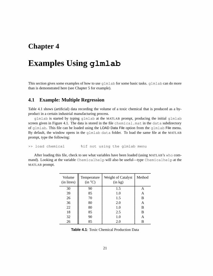
Table 4.1 shows (artificial) data recording the volume of a toxic chemical that is produced as a by-product in a certain industrial manufacturing process.
glmlab is started by typing glmlab at the MATLAB prompt, producing the initial glmlabscreen given in Figure 4.1. The data is stored in the file chemical.mat in the data subdirectoryof glmlab. This file can be loaded using the LOAD Data File option from the glmlab File menu.By default, the window opens in the glmlab data folder. To load the same file at the MATLAB
prompt, type the following:
>> load chemical %if not using the glmlab menu
After loading this file, check to see what variables have been loaded (using MATLAB’s who com-mand). Looking at the variable Chemicalhelp will also be useful—type Chemicalhelp at theMATLAB prompt.
Volume Temperature Weight of Catalyst Method(in litres) (in
�
C) (in kg)
30 90 1.5 A39 85 1.0 A26 70 1.5 B36 80 2.0 A22 80 1.0 B18 85 2.5 B32 90 1.0 A26 85 2.0 B
Table 4.1: Toxic Chemical Production Data
21

CHAPTER 4. EXAMPLES USING glmlab 22
Figure 4.1: The Initial glmlab Screen
>> ChemicalhelpChemicalhelp =The file chemical contains these variables:Cat: The weight of catalyst (in kg)Method: The method used to produce the chemical (qualitative)Temp: The temperature of the manufacturing processVol: The volume of toxic by-product produced.
Notice that variable names have been used with the first letter capitalised. This is a precaution againstusing names reserved by MATLAB or glmlab. (For example, length is a reserved word in MATLAB
used for defining the length of a vector. If length was used as a variable name, any MATLAB codethat used the function length would not work).
When defining variables, use names with capitalised first letters since mostMATLAB commands contain all lower case letters. ❢Remember that Method is a qualitative (or categorical) variable. To represent Method, a ‘1’
has been used for Method A and a ‘2’ for Method B.To begin fitting, start glmlab; the initial screen (Figure 4.1) should again appear. If glmlab is
already running, glmlab needs to be told that a new model is to be fitted. To do this, choose DeclareNew Model from the Options menu.
If glmlab is running and a new model is to be fitted or new data is to be loaded,choose Declare New Model from the Options menu. This clears all the internalsettings and resets the default options.
❢For demonstration purposes only, one variable at a time will be included in the model. The vari-
ables are then typed into their place: The response variable is Vol and the first covariate is Temp.When these are typed into the appropriate places in the glmlabWindow, and the FIT MODEL buttonis pressed, the following parameter estimates appears on the screen:
CHAPTER 4. EXAMPLES USING glmlab 23
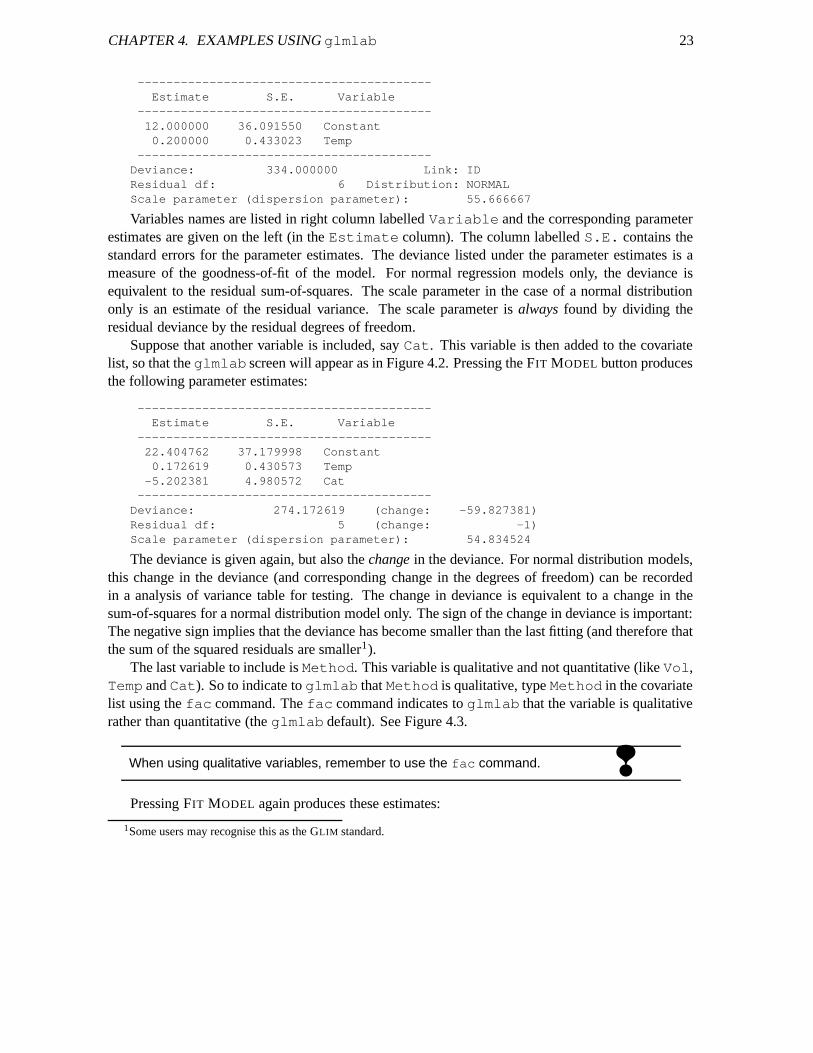
-----------------------------------------Estimate S.E. Variable
-----------------------------------------12.000000 36.091550 Constant0.200000 0.433023 Temp
-----------------------------------------Deviance: 334.000000 Link: IDResidual df: 6 Distribution: NORMALScale parameter (dispersion parameter): 55.666667
Variables names are listed in right column labelled Variable and the corresponding parameterestimates are given on the left (in the Estimate column). The column labelled S.E. contains thestandard errors for the parameter estimates. The deviance listed under the parameter estimates is ameasure of the goodness-of-fit of the model. For normal regression models only, the deviance isequivalent to the residual sum-of-squares. The scale parameter in the case of a normal distributiononly is an estimate of the residual variance. The scale parameter is always found by dividing theresidual deviance by the residual degrees of freedom.
Suppose that another variable is included, say Cat. This variable is then added to the covariatelist, so that the glmlab screen will appear as in Figure 4.2. Pressing the FIT MODEL button producesthe following parameter estimates:
-----------------------------------------Estimate S.E. Variable
-----------------------------------------22.404762 37.179998 Constant0.172619 0.430573 Temp
-5.202381 4.980572 Cat-----------------------------------------
Deviance: 274.172619 (change: -59.827381)Residual df: 5 (change: -1)Scale parameter (dispersion parameter): 54.834524
The deviance is given again, but also the change in the deviance. For normal distribution models,this change in the deviance (and corresponding change in the degrees of freedom) can be recordedin a analysis of variance table for testing. The change in deviance is equivalent to a change in thesum-of-squares for a normal distribution model only. The sign of the change in deviance is important:The negative sign implies that the deviance has become smaller than the last fitting (and therefore thatthe sum of the squared residuals are smaller1).
The last variable to include is Method. This variable is qualitative and not quantitative (like Vol,Temp and Cat). So to indicate to glmlab that Method is qualitative, type Method in the covariatelist using the fac command. The fac command indicates to glmlab that the variable is qualitativerather than quantitative (the glmlab default). See Figure 4.3.
When using qualitative variables, remember to use the fac command. ❢Pressing FIT MODEL again produces these estimates:
1Some users may recognise this as the GLIM standard.

CHAPTER 4. EXAMPLES USING glmlab 24
Figure 4.2: Variables Being Entered for Chemical Data
Figure 4.3: Entering Data Using the fac Command
CHAPTER 4. EXAMPLES USING glmlab 25
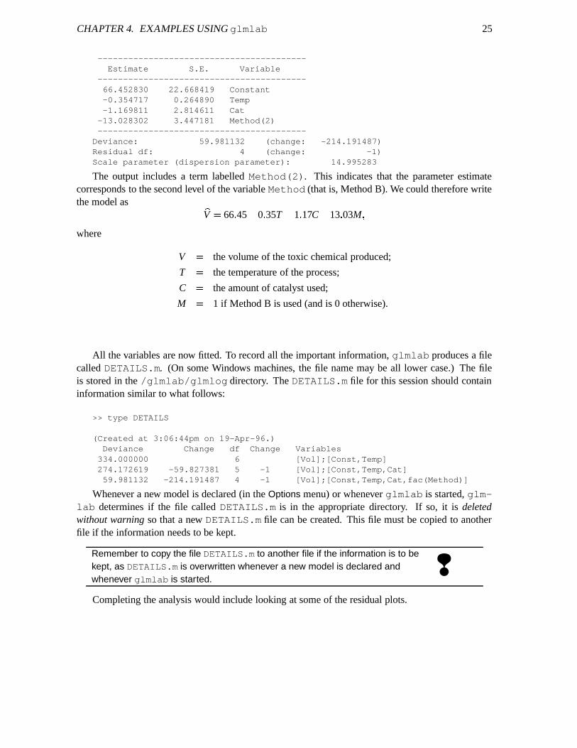
-----------------------------------------Estimate S.E. Variable
-----------------------------------------66.452830 22.668419 Constant-0.354717 0.264890 Temp-1.169811 2.814611 Cat
-13.028302 3.447181 Method(2)-----------------------------------------
Deviance: 59.981132 (change: -214.191487)Residual df: 4 (change: -1)Scale parameter (dispersion parameter): 14.995283
The output includes a term labelled Method(2). This indicates that the parameter estimatecorresponds to the second level of the variable Method (that is, Method B). We could therefore writethe model as �
V � 66 � 45�
0 � 35T�
1 � 17C�
13 � 03M �
where
V � the volume of the toxic chemical produced;
T � the temperature of the process;
C � the amount of catalyst used;
M � 1 if Method B is used (and is 0 otherwise).
All the variables are now fitted. To record all the important information, glmlab produces a filecalled DETAILS.m. (On some Windows machines, the file name may be all lower case.) The fileis stored in the /glmlab/glmlog directory. The DETAILS.m file for this session should containinformation similar to what follows:
>> type DETAILS
(Created at 3:06:44pm on 19-Apr-96.)Deviance Change df Change Variables
334.000000 6 [Vol];[Const,Temp]274.172619 -59.827381 5 -1 [Vol];[Const,Temp,Cat]59.981132 -214.191487 4 -1 [Vol];[Const,Temp,Cat,fac(Method)]
Whenever a new model is declared (in the Options menu) or whenever glmlab is started, glm-lab determines if the file called DETAILS.m is in the appropriate directory. If so, it is deletedwithout warning so that a new DETAILS.m file can be created. This file must be copied to anotherfile if the information needs to be kept.
Remember to copy the file DETAILS.m to another file if the information is to bekept, as DETAILS.m is overwritten whenever a new model is declared andwhenever glmlab is started.
❢Completing the analysis would include looking at some of the residual plots.
CHAPTER 4. EXAMPLES USING glmlab 26
Type of CounsellingStress Post Relationship Loss of Other
Abortion Breakdown Loved One TypesTrauma
Male 65 n/a 21 20 39Female 31 26 49 52 29Total 96 26 70 72 68
Table 4.2: Counselling Service Data
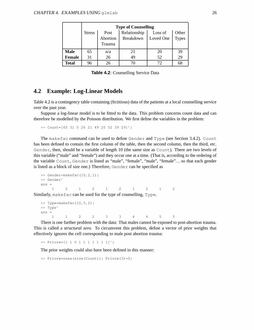
4.2 Example: Log-Linear Models
Table 4.2 is a contingency table containing (fictitious) data of the patients at a local counselling serviceover the past year.
Suppose a log-linear model is to be fitted to the data. This problem concerns count data and cantherefore be modelled by the Poisson distribution. We first define the variables in the problem:
>> Count=[65 31 0 26 21 49 20 52 39 29]’;
The makefac command can be used to define Gender and Type (see Section 3.4.2). Counthas been defined to contain the first column of the table, then the second column, then the third, etc.Gender, then, should be a variable of length 10 (the same size as Count). There are two levels ofthis variable (“male” and “female”) and they occur one at a time. (That is, according to the ordering ofthe variable Count, Gender is listed as “male”, “female”, “male”, “female”. . . so that each genderis listed as a block of size one.) Therefore, Gender can be specified as
>> Gender=makefac(10,2,1);>> Gender’ans =
1 2 1 2 1 2 1 2 1 2
Similarly, makefac can be used for the type of counselling, Type.
>> Type=makefac(10,5,2);>> Type’ans =
1 1 2 2 3 3 4 4 5 5
There is one further problem with the data: That males cannot be exposed to post-abortion trauma.This is called a structural zero. To circumvent this problem, define a vector of prior weights thateffectively ignores the cell corresponding to male post abortion trauma:
>> Priorw=[1 1 0 1 1 1 1 1 1 1]’;
The prior weights could also have been defined in this manner:
>> Priorw=ones(size(Count)); Priorw(3)=0;
CHAPTER 4. EXAMPLES USING glmlab 27
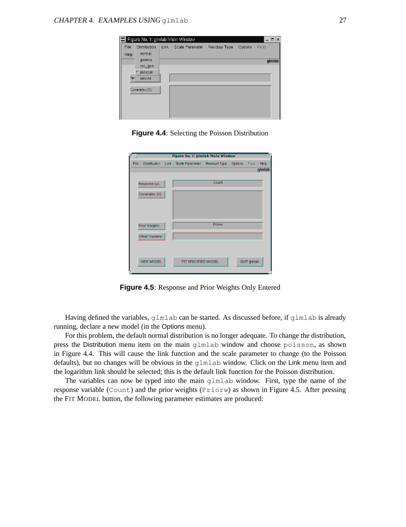
Figure 4.4: Selecting the Poisson Distribution
Figure 4.5: Response and Prior Weights Only Entered
Having defined the variables, glmlab can be started. As discussed before, if glmlab is alreadyrunning, declare a new model (in the Options menu).
For this problem, the default normal distribution is no longer adequate. To change the distribution,press the Distribution menu item on the main glmlab window and choose poisson, as shownin Figure 4.4. This will cause the link function and the scale parameter to change (to the Poissondefaults), but no changes will be obvious in the glmlab window. Click on the Link menu item andthe logarithm link should be selected; this is the default link function for the Poisson distribution.
The variables can now be typed into the main glmlab window. First, type the name of theresponse variable (Count) and the prior weights (Priorw) as shown in Figure 4.5. After pressingthe FIT MODEL button, the following parameter estimates are produced:

CHAPTER 4. EXAMPLES USING glmlab 28
-----------------------------------------Estimate S.E. Variable
-----------------------------------------3.607910 0.054882 Constant
-----------------------------------------Scaled deviance: 50.434008 Link: LOGResidual df: 8 Distribution: POISSONScale parameter (dispersion parameter): 1.000000
To add Gender to the covariate list, remember to use the fac command (as Gender is qualita-tive). Add fac(Gender) to the covariate list and press FIT MODEL again to produce new estimates:
-----------------------------------------Estimate S.E. Variable
-----------------------------------------3.590439 0.083044 Constant0.031231 0.110653 Gender(2)
-----------------------------------------Scaled Deviance: 50.354244 (change: -0.079764)Residual df: 7 (change: -1)Scale parameter (dispersion parameter): 1.000000
Now add the last variable, Type, to the covariate list so the list of variables in the Covariatearea includes fac(Gender) and fac(Type). Remember to use the fac command again becauseType is qualitative. Press the FIT MODEL button to produces new estimates.
-----------------------------------------Estimate S.E. Variable
-----------------------------------------3.817497 0.118512 Constant0.104671 0.114489 Gender(2)
-0.664071 0.227643 Type(2)-0.315853 0.157170 Type(3)-0.287682 0.155902 Type(4)-0.344840 0.158501 Type(5)
-----------------------------------------Scaled Deviance: 39.197423 (change: -11.156820)Residual df: 3 (change: -4)Scale parameter (dispersion parameter): 1.000000
The variable Type appears four times to indicate that there are five levels of this qualitativevariable (only four variables are needed for a five level factor to maintain full rank). These fourvariables correspond to levels two, three, four and five of the Type variable.
It is common to want to fit interaction terms during modelling. To fit interaction terms, glmlabuses the character @ (usually SHIFT-2 on the keyboard). See Section 3.4.3. In this problem, theinteraction between the two qualitative variables Gender and Type could be included. This canbe done in glmlab by entering the following string in the covariate section of the main glmlabwindow:
fac(Gender), fac(Type), fac(Gender)@fac(Type)
Notice that the fac command has been used again. Thus, interactions between variables can bespecified by separating the variables with the character @.
To define the interaction between variables in glmlab, use the @ characterbetween the interacting variables. Remember to still use fac for qualitativevariables.
❢
CHAPTER 4. EXAMPLES USING glmlab 29
Figure 4.6: Including an Interaction Term
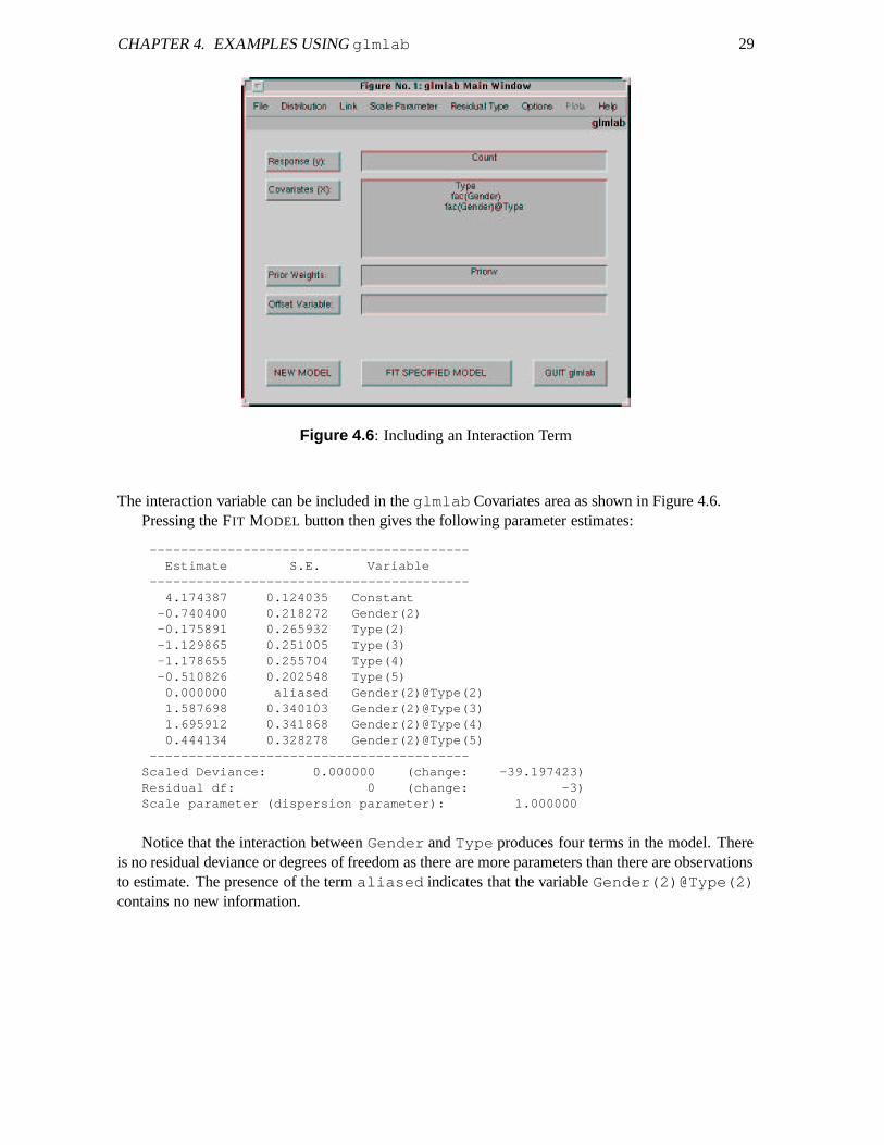
The interaction variable can be included in the glmlab Covariates area as shown in Figure 4.6.Pressing the FIT MODEL button then gives the following parameter estimates:
-----------------------------------------Estimate S.E. Variable
-----------------------------------------4.174387 0.124035 Constant
-0.740400 0.218272 Gender(2)-0.175891 0.265932 Type(2)-1.129865 0.251005 Type(3)-1.178655 0.255704 Type(4)-0.510826 0.202548 Type(5)0.000000 aliased Gender(2)@Type(2)1.587698 0.340103 Gender(2)@Type(3)1.695912 0.341868 Gender(2)@Type(4)0.444134 0.328278 Gender(2)@Type(5)
-----------------------------------------Scaled Deviance: 0.000000 (change: -39.197423)Residual df: 0 (change: -3)Scale parameter (dispersion parameter): 1.000000
Notice that the interaction between Gender and Type produces four terms in the model. Thereis no residual deviance or degrees of freedom as there are more parameters than there are observationsto estimate. The presence of the term aliased indicates that the variable Gender(2)@Type(2)contains no new information.
Chapter 5
Advanced Topics and Examples
This section contains some topics more complicated than those previously discussed. Further exam-ples are also given.
5.1 Offsets
Offsets are variables with known parameters. The name of the offset variable is listed in the Mainglmlabwindow in the appropriate area. The output on the screen and in the output file DETAILS.mindicates the name of the offset variable used.
5.2 Default Settings for Distributions
The error distribution type can be altered in glmlab via the Distributions menu item (see Section 4.2).The distributions available are: normal; inverse Gaussian; Poisson; binomial and gamma. Likewise,the type of link function used can be changed in the Link menu. The link functions available aresummarised in the Table 5.2. Each distribution has a default link function and scale parameter, assummarised in Table 5.1.
Only when the binomial distribution is chosen are the logit, probit and complementary log-loglinks available; at all other times, they appear are unavailable and dimmed in the Link menu.
5.3 Changing the Scale Parameter
Two types of scale parameter can be chosen: The mean deviance and a (positive) fixed value. Thedefaults are given in Table 5.1. When the scale parameter is estimated by the mean deviance, glmlabuses D
� �n
�r � where D is the deviance, n is the number of data points, and r is the number of
estimated parameters (n�
r is the number of degrees of freedom). The scale parameter can be fixedto any (positive) value; when the Fixed Value option is selected, the user is prompted for the value(whose default is 1).
Although the scale parameter is set to 1 by default for the binomial and Poisson distributions, itis not uncommon to use the mean deviance. This commonly occurs if under- or over-dispersion ispresent.
30

CHAPTER 5. ADVANCED TOPICS AND EXAMPLES 31
Error Default Link Default ScaleDistribution Function Parameter
Normal Identity Mean Devianceη � µ
Inverse Gaussian Inverse Quadratic Mean Devianceη � 1
�µ2
Poisson Logarithm Fixed (at 1)η � log µ
Binomial Logit Fixed (at 1)η � log � π � �
1�
π ���Gamma Reciprocal Mean Deviance
η � 1�µ
Table 5.1: Default Settings for Chosen Distributionsη is the linear predictor and µ is the mean (π in the binomial case).
Link Function Form
Identity η � µLogarithm η � logµReciprocal η � 1
�µ
Square Root η ��� µPower η � µp �
p non-zero)Logit η � log
�π
� �1�
π � �Complementary log-log η � log � � log
�1�
π ���Probit η � Φ � 1 � π �
Table 5.2: Link Functions in glmlabη is the linear predictor and µ is the mean. (π in the binomial case).
CHAPTER 5. ADVANCED TOPICS AND EXAMPLES 32
AG Positive AG NegativeWhite Blood Survival Time White Blood Survival Time
Count (WBC) (in weeks) Count (WBC) (in weeks)
2300 65 4400 56750 156 3000 65
4300 100 4000 172600 134 1500 76000 16 9000 16
10500 108 5300 2210000 121 10000 317000 4 19000 4
5400 39 27000 27000 143 28000 39400 56 31000 8
32000 26 26000 435000 22 21000 3
100000 1 79000 30100000 1 100000 452000 5 100000 43
100000 65
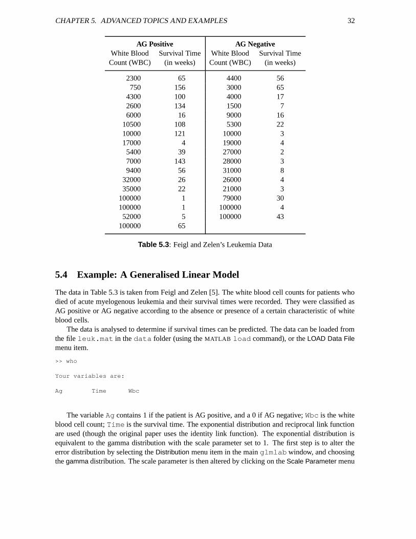
Table 5.3: Feigl and Zelen’s Leukemia Data
5.4 Example: A Generalised Linear Model
The data in Table 5.3 is taken from Feigl and Zelen [5]. The white blood cell counts for patients whodied of acute myelogenous leukemia and their survival times were recorded. They were classified asAG positive or AG negative according to the absence or presence of a certain characteristic of whiteblood cells.
The data is analysed to determine if survival times can be predicted. The data can be loaded fromthe file leuk.mat in the data folder (using the MATLAB load command), or the LOAD Data Filemenu item.
>> who
Your variables are:
Ag Time Wbc
The variable Ag contains 1 if the patient is AG positive, and a 0 if AG negative; Wbc is the whiteblood cell count; Time is the survival time. The exponential distribution and reciprocal link functionare used (though the original paper uses the identity link function). The exponential distribution isequivalent to the gamma distribution with the scale parameter set to 1. The first step is to alter theerror distribution by selecting the Distribution menu item in the main glmlab window, and choosingthe gamma distribution. The scale parameter is then altered by clicking on the Scale Parameter menu

CHAPTER 5. ADVANCED TOPICS AND EXAMPLES 33
Figure 5.1: Entering a Fixed Value for the Scale Parameter
Figure 5.2: Variables Entered for Example 5.4
item in the main glmlab window, and selecting Fixed Value. A new window appears; enter in thefixed value of the scale parameter (in this case, 1); see Figure 5.1. This has effectively selected theexponential distribution.
The original paper analyses the logarithm of the white blood cell counts, with the survival time,the AG factor, plus their interaction as covariates. The complete model can be fitted by typing in thevariables in the main glmlab window as shown in Figure 5.2. Note the use of the fac command(because Ag is qualitative) and the @ symbol.
Pressing the FIT MODEL button produces the following estimates:
------------------------------------------------------------Estimate S.E. Variable
------------------------------------------------------------8.478205 1.655453 Constant
-0.481829 0.173635 log(Wbc)-4.137813 2.570290 Ag(2)0.328110 0.266888 log(Wbc)@Ag(2)
------------------------------------------------------------Scaled Deviance: 38.554607 (change: +0.000000)Residual df: 29 (change: +0)Scale parameter (dispersion parameter): 1.000000
CHAPTER 5. ADVANCED TOPICS AND EXAMPLES 34
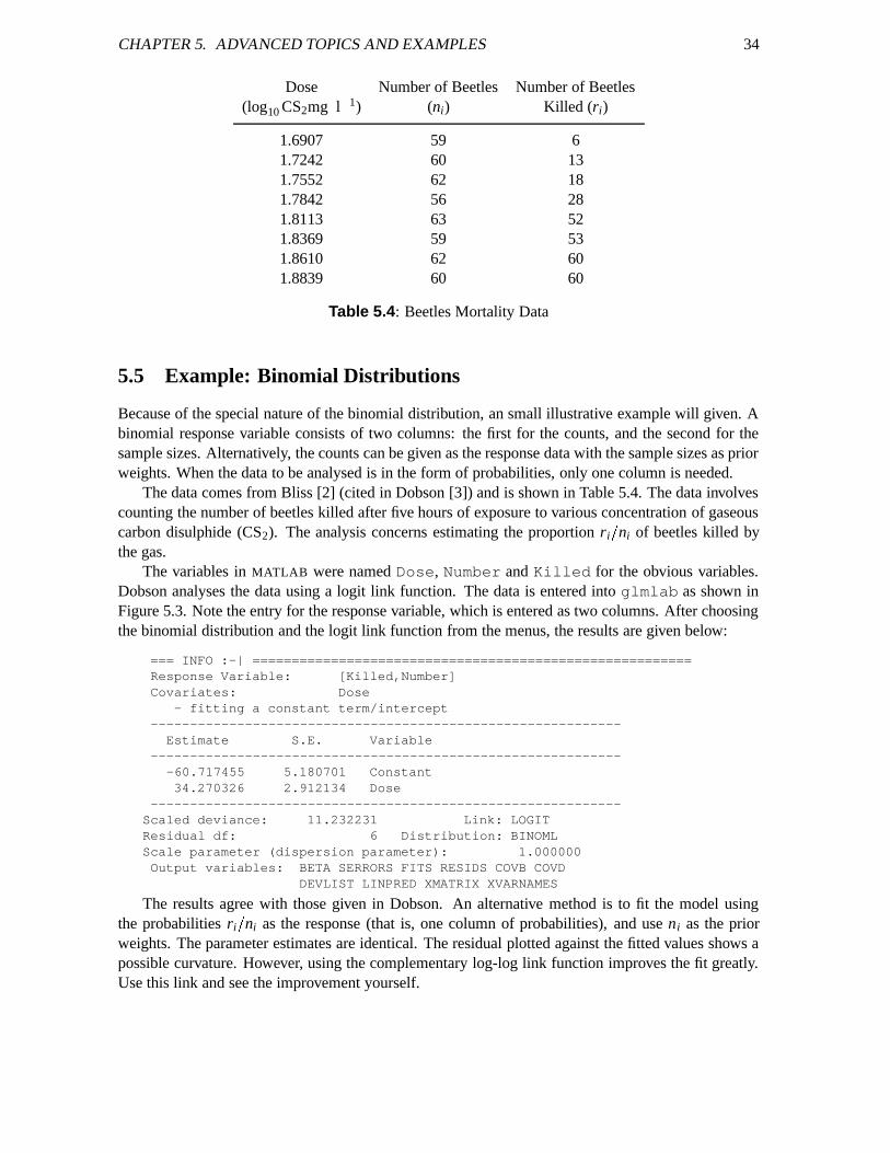
Dose Number of Beetles Number of Beetles(log10 CS2mg l � 1) (ni) Killed (ri)
1.6907 59 61.7242 60 131.7552 62 181.7842 56 281.8113 63 521.8369 59 531.8610 62 601.8839 60 60
Table 5.4: Beetles Mortality Data
5.5 Example: Binomial Distributions
Because of the special nature of the binomial distribution, an small illustrative example will given. Abinomial response variable consists of two columns: the first for the counts, and the second for thesample sizes. Alternatively, the counts can be given as the response data with the sample sizes as priorweights. When the data to be analysed is in the form of probabilities, only one column is needed.
The data comes from Bliss [2] (cited in Dobson [3]) and is shown in Table 5.4. The data involvescounting the number of beetles killed after five hours of exposure to various concentration of gaseouscarbon disulphide (CS2). The analysis concerns estimating the proportion ri
�ni of beetles killed by
the gas.The variables in MATLAB were named Dose, Number and Killed for the obvious variables.
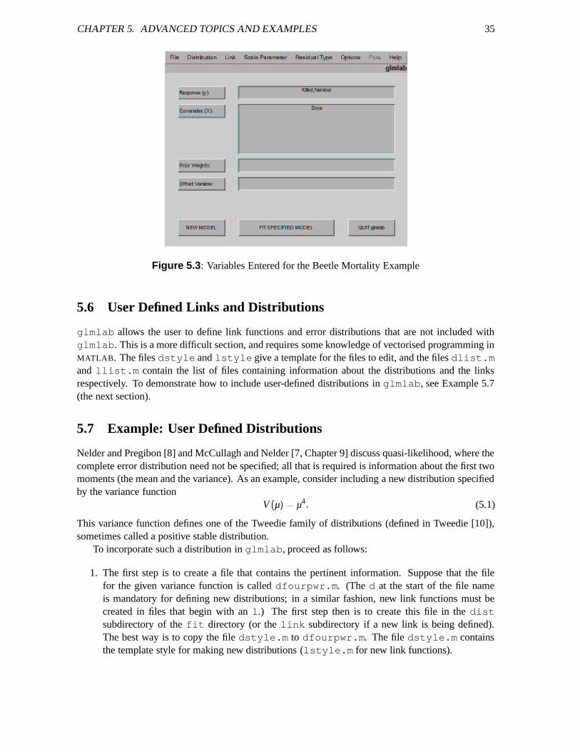
Dobson analyses the data using a logit link function. The data is entered into glmlab as shown inFigure 5.3. Note the entry for the response variable, which is entered as two columns. After choosingthe binomial distribution and the logit link function from the menus, the results are given below:
=== INFO :-| ========================================================Response Variable: [Killed,Number]Covariates: Dose
- fitting a constant term/intercept------------------------------------------------------------
Estimate S.E. Variable------------------------------------------------------------
-60.717455 5.180701 Constant34.270326 2.912134 Dose
------------------------------------------------------------Scaled deviance: 11.232231 Link: LOGITResidual df: 6 Distribution: BINOMLScale parameter (dispersion parameter): 1.000000Output variables: BETA SERRORS FITS RESIDS COVB COVD
DEVLIST LINPRED XMATRIX XVARNAMES
The results agree with those given in Dobson. An alternative method is to fit the model usingthe probabilities ri
�ni as the response (that is, one column of probabilities), and use ni as the prior
weights. The parameter estimates are identical. The residual plotted against the fitted values shows apossible curvature. However, using the complementary log-log link function improves the fit greatly.Use this link and see the improvement yourself.
CHAPTER 5. ADVANCED TOPICS AND EXAMPLES 35
Figure 5.3: Variables Entered for the Beetle Mortality Example
5.6 User Defined Links and Distributions
glmlab allows the user to define link functions and error distributions that are not included withglmlab. This is a more difficult section, and requires some knowledge of vectorised programming inMATLAB. The files dstyle and lstyle give a template for the files to edit, and the files dlist.mand llist.m contain the list of files containing information about the distributions and the linksrespectively. To demonstrate how to include user-defined distributions in glmlab, see Example 5.7(the next section).
5.7 Example: User Defined Distributions
Nelder and Pregibon [8] and McCullagh and Nelder [7, Chapter 9] discuss quasi-likelihood, where thecomplete error distribution need not be specified; all that is required is information about the first twomoments (the mean and the variance). As an example, consider including a new distribution specifiedby the variance function
V�µ � � µ4
� (5.1)
This variance function defines one of the Tweedie family of distributions (defined in Tweedie [10]),sometimes called a positive stable distribution.
To incorporate such a distribution in glmlab, proceed as follows:
1. The first step is to create a file that contains the pertinent information. Suppose that the filefor the given variance function is called dfourpwr.m. (The d at the start of the file nameis mandatory for defining new distributions; in a similar fashion, new link functions must becreated in files that begin with an l.) The first step then is to create this file in the distsubdirectory of the fit directory (or the link subdirectory if a new link is being defined).The best way is to copy the file dstyle.m to dfourpwr.m. The file dstyle.m containsthe template style for making new distributions (lstyle.m for new link functions).

CHAPTER 5. ADVANCED TOPICS AND EXAMPLES 36
2. The second step is to edit the file named dfourpwr.m using any text editor. Near the end ofthe file is a section with the following information:
%Calculateif strcmp(what,’varfn’),
%%%In here, you need lines to find the variance function%%%from mu and y.%%%The section should return the variance function as answ
elseif strcmp(what,’scdev’);%%%In here, you need lines to find the scaled deviance%%%from mu and y.%%%The section should return the scaled deviance as answ
end;
It should be clear that there are two sections to alter: One section requires information aboutthe variance function, and the other about the deviance. For the variance function given inEquation (5.1), the MATLAB equivalent code is
answ = mu .ˆ 4;This line should be entered into the section requiring information about the variance function.The deviance can be found from the integral
D�y � µ � � �
2 � µ
y
y�
uV
�u � du �
which, for the given variance function, is
D � 16y2 � y
3µ3
� 12µ2 �
The equivalent MATLAB code isansw=1/(6*yˆ2) + ( y./(3*mu.ˆ3) ) - ( 1/(2*mu.ˆ2) );
This line of code is placed in the section requiring the deviance. Now glmlab has the infor-mation that it requires; it now needs to know to use the file dfourpwr.m.
3. In the dist directory, there is a file called dlist.m which lists all the files that containinformation about distributions. (There is a corresponding file llist.m for the link functions.)Add a new line to the end of this file that says only
dfourpwr.m
4. All the required tasks have been completed. Next time glmlab is started, there should be adistribution named fourpwr at the bottom of list of distributions.
A similar procedure is used for defining new link functions, but the corresponding files in thelink subdirectory of the fit directory are used. Adding new distribution or link functions is notrecommended unless the user knows the use of the distribution or link function, as odd results mayeventuate otherwise.
5.8 The Default Data Directory
As discussed in sections 4.1 and 5.4, data can be loaded with the graphical interface by selectingLOAD Data File under the file menu. The default data directory is initially glmlab/data. This can,
CHAPTER 5. ADVANCED TOPICS AND EXAMPLES 37
Figure 5.4: The Fitting Parameters Window
however, be easily changed. In the glmlab/data directory, there is a file named dummydta.mwhich contains basically nothing; the sole purpose of the file is to define the default data directory.To have a different default directory, simply move this file into the appropriate directory. Next timethe graphical load data window appears, the default directory will be the directory where this file islocated.
5.9 npplot
This function can be used to produce a normal probability plot (which is useful for checking thenormality of the data). It is called by the glmlab plotting window, but can also be used outside ofglmlab. The general form of the command is
npplot(y,s);where y is the data and s is 0 to include a dotted line corresponding to the standard normal distribution,and is 1 too include a dotted line corresponding to a normal distribution with the same mean andvariance as the given data, y.
The Statistics Toolbox of MATLAB has its own function for plotting a normal probability plot.
5.10 Changing the Fitting Parameters
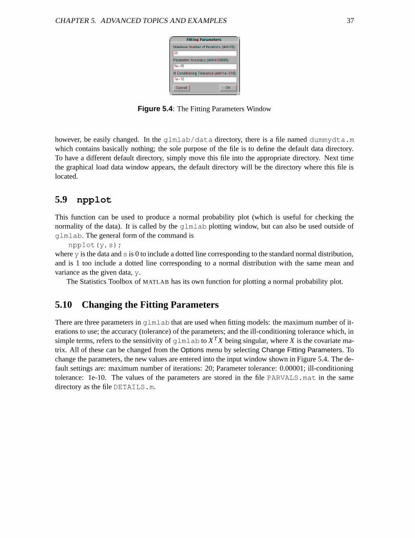
There are three parameters in glmlab that are used when fitting models: the maximum number of it-erations to use; the accuracy (tolerance) of the parameters; and the ill-conditioning tolerance which, insimple terms, refers to the sensitivity of glmlab to X T X being singular, where X is the covariate ma-trix. All of these can be changed from the Options menu by selecting Change Fitting Parameters. Tochange the parameters, the new values are entered into the input window shown in Figure 5.4. The de-fault settings are: maximum number of iterations: 20; Parameter tolerance: 0.00001; ill-conditioningtolerance: 1e-10. The values of the parameters are stored in the file PARVALS.mat in the samedirectory as the file DETAILS.m.

References
[1] Murray Aitken, Dorothy Anderson, Brian Francis, and John Hinde. Statistical Modelling inGLIM. Number 4 in Oxford Statistical Sciences Series. Oxford University Press, 1990.
[2] C. I. Bliss. The calculation of the dosage-mortality curve. The Annals of Applied Biology,22:134–167, 1935.
[3] Annette J. Dobson. An Introduction to Statistical Modelling. Chapman and Hall, 1983.
[4] Peter K. Dunn and Gordon K. Smyth. Randomized quantile residuals. The Journal of Compu-tational and Graphical Statistics, 5:1–10, September 1996.
[5] Polly Feigl and Marvin Zelen. Estimation of exponential survival probabilities with concomitantinformation. Biometrics, 21:826–838, December 1965.
[6] Brian Francis, Mick Green, and Clive Payne. The GLIM System: generalised linear interactivemodelling. Release 4 Manual. Clarendon Press, 1993.
[7] P. McCullagh and J. A. Nelder. Generalized Linear Models. Number 37 in Monographs onStatistics and Applied Probability. Chapman and Hall, second edition, 1994.
[8] J. A. Nelder and D. Pregibon. An extended quasi-likelihood function. Biometrika, 74(2):221–232, 1987.
[9] Statistical Sciences, Inc. S-PLUS User’s Manual, Version 3.3 for Windows, 1995.
[10] M. C. K. Tweedie. An index which distinguishes between some important exponential families.In Proceedings of the Indian Statistical Institute Golden Jubilee International Conference onStatistics: Applications and New Directions, pages 579–604, December 1981.
38
Index
Entries in typewriter font refer to MATLAB or glm-lab commands.
Symbols@ . . . . . . . . . . . . . . . . . . . . . . . . . . . . . . . . . . . . see interaction’ . . . . . . . . . . . . . . . . . . . . . . . . . . . . . . . . . . . . . .see transpose... . . . . . . . . . . . . . . . . . . . . . . . . . . . . see line continuation. . . . . . . . . . . . . . . . . . . . . . . . . . . . . . . . . . . . . . . . . see period: . . . . . . . . . . . . . . . . . . . . . . . . . . . . . . . . . . . . . . . . . see colon; . . . . . . . . . . . . . . . . . . . . . . . . . . . . . . . . . . . . . see semicolonˆ . . . . . . . . . . . . . . . . . . . . . . . . . . . . . . . . . . . . . . . . . . see caret
� . . . . . . . . . . . . . . . . . . . . . . . . . . . . . . . . . . . . . . . see asterisk% . . . . . . . . . . . . . . . . . . . . . . . . . . . . . . . . . . . . . see comments
Aaliased . . . . . . . . . . . . . . . . . . . . . . . . . . . . . . . . . . . . . . . . . . 29analysis of variance . . . . . . . . . . . . . . . . . . . . . . . . . . . . . . . 23ans . . . . . . . . . . . . . . . . . . . . . . . . . . . . . . . . . . . . . . . . . . . . .10asterisk . . . . . . . . . . . . . . . . . . . . . . . . . . . . . . . . . . . . . 5, 8, 11axis . . . . . . . . . . . . . . . . . . . . . . . . . . . . . . . . . . . . . . . . 10, 11
Ccaret . . . . . . . . . . . . . . . . . . . . . . . . . . . . . . . . . . . . . . . . . 11, 36categorical . . . . . . . . . . . . . . . . . . . . . . . . . . . . see qualitativeclear . . . . . . . . . . . . . . . . . . . . . . . . . . . . . . . . . . . . . . . . . . . 8colon . . . . . . . . . . . . . . . . . . . . . . . . . . . . . . . . . . . . . . . 7–9, 11comments . . . . . . . . . . . . . . . . . . . . . . . . . . . . . . . . . . . . . 9, 36complementary log-log . . . . . . . . . . . . . . . . . . . . . . . see linkcontingency table . . . . . . . . . . . . . . . . . . . . . . . . . . . . . . . . . 26cos . . . . . . . . . . . . . . . . . . . . . . . . . . . . . . . . . . . . . . . . . . . . . . 6covariates . . . . . . . . . . . . . . . . . . . . . . . . . . . . . 22, 23, 28, 29.cshrc . . . . . . . . . . . . . . . . . . . . . . . . . . . . . . . . . . . . . . . . . . 3
Ddata files . . . . . . . . . . . . . . . . . . . . . . . . . . . . . . . . . . . . . . . 7–8
loading . . . . . . . . . . . . . . . . . . . . . . . . . . . . . . . 7, 32, 36saving . . . . . . . . . . . . . . . . . . . . . . . . . . . . . . . . . . . . . . . 8
defaultdata directory . . . . . . . . . . . . . . . . . . . . . . . . . . . . 12, 36deviance . . . . . . . . . . . . . . . . . . . . . . . . . . . . . . . . . . . .31distribution . . . . . . . . . . . . . . . . . . . . . . . . . . . . . . . . . 31link . . . . . . . . . . . . . . . . . . . . . . . . . . . . . . . . . . . . . . . . 31parameters . . . . . . . . . . . . . . . . . . . . . . . . . . . . . . . . . . 37
degrees of freedom . . . . . . . . . . . . . . . . . . . . . . . . 23, 29, 30
DETAILS.m . . . . . . . . . . . . . . . . . . . . . . . . . . . . . . . . . 25, 30deviance . . . . . . . . . . . . . . . . . . . . . . . . . . . . . . 23, 29–31, 36diary . . . . . . . . . . . . . . . . . . . . . . . . . . . . . . . . . . . . . . . . . . 10distributions . . . . . . . . . . . . . . . . . . . . . . . . . . . . . . .30, 31, 35
binomial . . . . . . . . . . . . . . . . . . . . . . . . . . . . . 14, 30, 34changing . . . . . . . . . . . . . . . . . . . . . . . . . . . . . . . . . . . 30exponential . . . . . . . . . . . . . . . . . . . . . . . . . . . . . . 32–33gamma . . . . . . . . . . . . . . . . . . . . . . . . . . . 14, 30, 32–33inverse Gaussian . . . . . . . . . . . . . . . . . . . . . . . . . 14, 30menu . . . . . . . . . . . . . . . . . . . . . . . . . 14, 27, 30, 32, 36normal . . . . . . . . . . . . . . . . . . . . . . . .14, 21–25, 30, 37Poisson . . . . . . . . . . . . . . . . . . . . . . . . . . . . . . 14, 25–30user-defined . . . . . . . . . . . . . . . . . . . . . . . . . . . . . 35–36
dlist.m . . . . . . . . . . . . . . . . . . . . . . . . . . . . . . . . . . . . . . . 36dstyle . . . . . . . . . . . . . . . . . . . . . . . . . . . . . . . . . . . . . . . . .35
Eexp . . . . . . . . . . . . . . . . . . . . . . . . . . . . . . . . . . . . . . . . . . . . .11exponential distribution . . . . . . . . . . . . . . . see distributionseye . . . . . . . . . . . . . . . . . . . . . . . . . . . . . . . . . . . . . . . . . . . . .10
Ffac . . . . . . . . . . . . . . . . . . . . . . . . . . . . . . . . . . . . . . 23, 28, 33file
menu . . . . . . . . . . . . . . . . . . . . . . . . . . . . . . . . . . . . . . .32files . . . . . . . . . . . . . . . . . . . . . . . . . . . . . . . . . . . .see data files
Ggamma distribution . . . . . . . . . . . . . . . . . . see distributionsgeneralised linear model . . . . . . . . . . . . . . . . . . . . . 1, 32–34GLIM . . . . . . . . . . . . . . . . . . . . . . . . . . . . . . . . . . . . . . . . . 1, 19glmlab
changing options . . . . . . . . . . . . . . . . . . . . . . . . . 14, 27Home Page . . . . . . . . . . . . . . . . . . . . . . . . . . . . . . . . viiiinstalling . . . . . . . . . . . . . . . . . . . . . . . . . . . . . . . . . . 1–3Main Window . . . . . . . . . . . . . . . . . . . . . . . . 13, 22, 30output explained . . . . . . . . . . . . . . . . . . . . . . 23, 25, 29
Hhelp . . . . . . . . . . . . . . . . . . . . . . . . . . . . . . . . . . . . . . . . . . 6, 9help menus . . . . . . . . . . . . . . . . . . . . . . . . . . . . . . . . . . . . . . 16helpdesk . . . . . . . . . . . . . . . . . . . . . . . . . . . . . . . . . . . . . . . 6hist . . . . . . . . . . . . . . . . . . . . . . . . . . . . . . . . . . . . . . . . . . . . 1histograms . . . . . . . . . . . . . . . . . . . . . . . . . . . . . 16, see hist
39
INDEX 40
Home Page (World Wide Web) . . . . . . . . . . . . . . . . . . . . viii
Ii (
�� 1) . . . . . . . . . . . . . . . . . . . . . . . . . . . . . . . . . . . . . . . . 11
identity link . . . . . . . . . . . . . . . . . . . . . . . . . . . . . . . . . see linkInf (∞) . . . . . . . . . . . . . . . . . . . . . . . . . . . . . . . . . . . . . . . . . 11installing glmlab . . . . . . . . . . . . see glmlab, installinginteraction . . . . . . . . . . . . . . . . . . . . . . . . . . . . . . . . 28–29, 33inv . . . . . . . . . . . . . . . . . . . . . . . . . . . . . . . . . . . . . . . . . . . . . . 5inverse Gaussian distribution . . . . . . . . . . see distributionsisstr . . . . . . . . . . . . . . . . . . . . . . . . . . . . . . . . . . . . . . . . . . 36iterations
default number . . . . . . . . . . . . . . . . . . . . . . . . . . . . . . 15displaying . . . . . . . . . . . . . . . . . . . . . . . . . . . . . . . . . . 15maximum number . . . . . . . . . . . . . . . . . . . . . . . . . . . 37
Llabels . . . . . . . . . . . . . . . . . . . . . see xlabel and ylabelline continuation . . . . . . . . . . . . . . . . . . . . . . . . . . . . . . . 2, 10linear predictor . . . . . . . . . . . . . . . . . . . . . . . . . . . . . . . . . . . 31link . . . . . . . . . . . . . . . . . . . . . . . . . . . . . . . . . . . 27, 30, 31, 35
changing . . . . . . . . . . . . . . . . . . . . . . . . . . . . . . . . . . . 31complementary log-log . . . . . . . . . . . . . . . .14, 31, 34default . . . . . . . . . . . . . . . . . . . . . . . . . . . . . . . . . . . . . 31identity . . . . . . . . . . . . . . . . . . . . . . . . . . 14, 21–25, 31logarithm. . . . . . . . . . . . . . . . . . . . . . . . .14, 25–29, 31logit . . . . . . . . . . . . . . . . . . . . . . . . . . . . . . . . . 14, 31, 34menu . . . . . . . . . . . . . . . . . . . . . . . . . . . . 14, 27, 30, 31power . . . . . . . . . . . . . . . . . . . . . . . . . . . . . . . . . . .14, 31probit . . . . . . . . . . . . . . . . . . . . . . . . . . . . . . . . . . . 14, 31reciprocal . . . . . . . . . . . . . . . . . . . . . . . . . . . . 14, 31–33square root . . . . . . . . . . . . . . . . . . . . . . . . . . . . . . 14, 31user-defined . . . . . . . . . . . . . . . . . . . . . . . . . . . . . 35–36
llist.m . . . . . . . . . . . . . . . . . . . . . . . . . . . . . . . . . . . . . . . 36load . . . . . . . . . . . . . . . . . . . . . . . . . . . . . . . . . . . . . . . . . . . . 7log-linear models . . . . . . . . . . . . . . . . . . . . . . . . . . . . . 25–29logarithm . . . . . . . . . . . . . . . . . . . . . . . . . . . . . . . . . . . . . . . . 33
of negative numbers . . . . . . . . . . . . . . . . . . . . . . . . . 11logarithm link . . . . . . . . . . . . . . . . . . . . . . . . . . . . . . . see linklogistic link . . . . . . . . . . . . . . . . . . . . . . . . . . . . see link, logitlogit link . . . . . . . . . . . . . . . . . . . . . . . . . . . . . . . . . . . . see linklookfor . . . . . . . . . . . . . . . . . . . . . . . . . . . . . . . . . . . . . . . . 6lstyle . . . . . . . . . . . . . . . . . . . . . . . . . . . . . . . . . . . . . . . . .35
Mmakefac . . . . . . . . . . . . . . . . . . . . . . . . . . . . . . . . . . . . . . . 26MATLAB . . . . . . . . . . . . . . . . . . . . . . . . . . . . . . . . . . . 4–11, 35matlabrc.m . . . . . . . . . . . . . . . . . . . . . . . . . . . . . . . . . . . . 2mean . . . . . . . . . . . . . . . . . . . . . . . . . . . . . . . . . . . . . . . . . . . . 1median . . . . . . . . . . . . . . . . . . . . . . . . . . . . . . . . . . . . . . . . . . 1menus
distribution . . . . . . . . . . . . . . . . . . . .14, 27, 30, 32, 36file . . . . . . . . . . . . . . . . . . . . . . . . . . . . . . . . . . 12, 21, 32help . . . . . . . . . . . . . . . . . . . . . . . . . . . . . . . . . . . . . . . . 16link . . . . . . . . . . . . . . . . . . . . . . . . . . . . . . . . . 14, 27, 30
options . . . . . . . . . . . . . . . . . . . . . . . . . . . . . . . . . .14, 22residual . . . . . . . . . . . . . . . . . . . . . . . . . . . . . . . . . . . . 14scale parameter . . . . . . . . . . . . . . . . . . . . . . . 14, 30, 32
more . . . . . . . . . . . . . . . . . . . . . . . . . . . . . . . . . . . . . . . . . . . . 6
Nnew model . . . . . . . . . . . . . . . . . . . . . . . . . . . . . . . . . . . . . . . 22normal distribution . . . . . . . . . . . . . . . . . . . see distributionsnormal probability plot . . . . . . . . . . . . . . . . . . . . . . . . . . . .37npplot . . . . . . . . . . . . . . . . . . . . . . . . . . . . . . . . . . . . . . . . .37
Ooffset . . . . . . . . . . . . . . . . . . . . . . . . . . . . . . . . . . . . . . . . . . . .30ones . . . . . . . . . . . . . . . . . . . . . . . . . . . . . . . . . . . . . . . . 10, 26options menu . . . . . . . . . . . . . . . . . . . . . . . . . . . . . . . . . 14, 22output from glmlab explained . . . see glmlab, output
explainedover-dispersion . . . . . . . . . . . . . . . . . . . . . . . . . . . . . . . . . . . 30
Pparameter estimates . . . . . . . . . . . . . . . . . . . . . . . . 23, 25, 29
known. . . . . . . . . . . . . . . . . . . . . . . . . . . . . . . . . . . . . .30parvals.mat . . . . . . . . . . . . . . . . . . . . . . . . . . . . . . . . . . 37period . . . . . . . . . . . . . . . . . . . . . . . . . . . . . . . . . . . . . 5, 11, 36pi (π) . . . . . . . . . . . . . . . . . . . . . . . . . . . . . . . . . . . . . . . . . . . . 7plot . . . . . . . . . . . . . . . . . . . . . . . . . . . . . . . . . . . . . . . . . 8–10plots . . . . . . . . . . . . . . . . . . . . . . . . . . . . . . . . . . . . . . . . . . . . 27Poisson distribution . . . . . . . . . . . . . . . . . . see distributionspower link . . . . . . . . . . . . . . . . . . . . . . . . . . . . . . . . . . see linkprint . . . . . . . . . . . . . . . . . . . . . . . . . . . . . . . . . . . . . . . . . . . . 10print . . . . . . . . . . . . . . . . . . . . . . . . . . . . . . . . . . . . . . . . . . 10printers . . . . . . . . . . . . . . . . . . . . . . . . . . . . . . . . . . . . . . . . . . 10prior weights . . . . . . . . . . . . . . . . . . . . . . . . . . . . . . 26–27, 34probit link . . . . . . . . . . . . . . . . . . . . . . . . . . . . . . . . . . see linkpropedit . . . . . . . . . . . . . . . . . . . . . . . . . . . . . . . . . . . . . . 10
Qqualitative . . . . . . . . . . . . . . . . . . . . . . . . . . . . . 22, 23, 28, 33quantitative . . . . . . . . . . . . . . . . . . . . . . . . . . . . . . . . . . . . . . 23quasi-likelihoods . . . . . . . . . . . . . . . . . . . . . . . . . . . . . . . . . 35
Rradians . . . . . . . . . . . . . . . . . . . . . . . . . . . . . . . . . . . . . . . . . . . 6randn . . . . . . . . . . . . . . . . . . . . . . . . . . . . . . . . . . . . . . . . . . . 9reciprocal link . . . . . . . . . . . . . . . . . . . . . . . . . . . . . . . see linkregression
multiple . . . . . . . . . . . . . . . . . . . . . . . . . . . . . . . . . 21–25residual sum-of-squares . . . . . . . . . . . . . . . . . . . . . . . . . . . 23residuals . . . . . . . . . . . . . . . . . . . . . . . . . . . . . . . . . . . . . 23, 25
menu . . . . . . . . . . . . . . . . . . . . . . . . . . . . . . . . . . . . . . .14response variable. . . . . . . . . . . . . . . . . . . . . . . . . . . . . .22, 27
INDEX 41
Ssave . . . . . . . . . . . . . . . . . . . . . . . . . . . . . . . . . . . . . . . . . . . . 8scale parameter . . . . . . . . . . . . . . . . . . . . . . . . 23, 27, 30–32
menu . . . . . . . . . . . . . . . . . . . . . . . . . . . . . . . . 14, 30, 32semicolon . . . . . . . . . . . . . . . . . . . . . . . . . . . . . . . . . . . . . . 4, 9settings . . . . . . . . . . . . . . . . . . . . . . . . . . . . . . . . . . see options
changing . . . . . . . . . . . . . . . . . . . . . . . . . . . . . . . . . . . 37defaults . . . . . . . . . . . . . . . . . . . . . . . . . . . . . . . . . . . . 37
size . . . . . . . . . . . . . . . . . . . . . . . . . . . . . . . . . . . . . . . . 10, 26sort . . . . . . . . . . . . . . . . . . . . . . . . . . . . . . . . . . . . . . . . . . . 10square root link . . . . . . . . . . . . . . . . . . . . . . . . . . . . . . see linkstandard errors . . . . . . . . . . . . . . . . . . . . . . . . . . . . . . . . . . . 23Statistics Toolbox. . . . . . . . . . . . . . . . . . . . . . . . . . . . . . . . . .1std . . . . . . . . . . . . . . . . . . . . . . . . . . . . . . . . . . . . . . . . . . . . . . 1strcmp . . . . . . . . . . . . . . . . . . . . . . . . . . . . . . . . . . . . . . . . .36
Ttitle . . . . . . . . . . . . . . . . . . . . . . . . . . . . . . . . . . . . . see titletitle . . . . . . . . . . . . . . . . . . . . . . . . . . . . . . . . . . . . . . . . 9, 11Toolbox, Statistics . . . . . . . . . . . . . . . . . . . . . . . . . . . . . . . . . 1transpose . . . . . . . . . . . . . . . . . . . . . . . . . . . . . . . . . . . .4, 5, 26type . . . . . . . . . . . . . . . . . . . . . . . . . . . . . . . . . . . . . . . . . . . 25
Uunder-dispersion . . . . . . . . . . . . . . . . . . . . . . . . . . . . . . . . . 30
Vvariance function. . . . . . . . . . . . . . . . . . . . . . . . . . . . . .35, 36vector . . . . . . . . . . . . . . . . . . . . . . . . . . . . . . . . . . . . . . . . . . 8, 9
Wwho . . . . . . . . . . . . . . . . . . . . . . . . . . . . . . . . . . . . . . . . . . 8, 21whos . . . . . . . . . . . . . . . . . . . . . . . . . . . . . . . . . . . . . . . . . . . . 8
Xxlabel . . . . . . . . . . . . . . . . . . . . . . . . . . . . . . . . . . . . . . 9, 11
Yylabel . . . . . . . . . . . . . . . . . . . . . . . . . . . . . . . . . . . . . . 9, 11
Zzeros . . . . . . . . . . . . . . . . . . . . . . . . . . . . . . . . . . . . . . . . . . 10
Copyright © 2022 FDOKUMEN