Generalised Dynamic Ordinals – universal measures

for implicit computational complexity

Arnold Beckmann∗

University of Wales Swansea

Singleton Park

Swansea SA2 8PP, UK

A.Beckmann@swansea.ac.uk

June 29, 2005

Abstract

We extend the definition of dynamic ordinals to generalised dy-namic ordinals. We compute generalised dynamic ordinals of all frag-ments of relativised bounded arithmetic by utilising methods fromBoolean complexity theory, similar to Krajıcek in [14]. We indicate therole of generalised dynamic ordinals as universal measures for implicitcomputational complexity. I.e., we describe the connections betweengeneralised dynamic ordinals and witness oracle Turing machines forbounded arithmetic theories. In particular, through the determinationof generalised dynamic ordinals we re-obtain well-known independenceresults for relativised bounded arithmetic theories.

Keywords: Bounded arithmetic; dynamic ordinals; universal mea-sures; witness oracle Turing machines; implicit computational com-plexity; independence results; Hastad’s Switching Lemmas; cut-reduction by switching.

MSC: 03F20; 03F30, 68Q15, 68R99.

1 Introduction

Implicit computational complexity denotes the collection of approaches tocomputational complexity which define and classify the complexity of com-putations without direct reference to an underlying machine model. Theseapproaches are formal systems which cover a wide range, including applica-tive functional programming languages, linear logic, bounded arithmeticand finite model theory (cf. [17]). In this paper, we contribute to the idea

∗This work has been supported by a Marie Curie Individual Fellowship #HPMF-CT-2000-00803 from the European Commission.

1

of characterising the computational complexity of such formal systems byuniversal measures, such that the formal systems describe exactly the samecomplexity class, if and only if they agree in their universal measures. Ingeneral, we aim at connections which can be represented as follows:

complexity class oo // formal systems

universal measure²²

OOjjUUUUUUUUUUUUUUUUUUUUUUUU

Many formal systems admit such kind of universal measures. For exam-ple, in case of “strong” implicit computational complexity, e.g. for number-theoretic functions which are computable by primitive recursive functionalsin finite types, so-called proof-theoretic ordinals have proven useful as uni-versal measures of proof and computation (and also consistency) strength(cf. [19]). With respect to our general picture this situation can be repre-sented as follows:

PA

primitive recursive in all finite typesrr

22dddddddddddddddddddddddddddddddddddoo //

kk

++VVVVVVVV

VVVVVVVV

VVACA0

Godel’s T

proof-theoretic ordinal ε0¼¼

YY222222222222222 ²²

OO

­­

JJ¸¸¸¸¸¸¸¸¸¸¸¸¸¸¸¸¸¸¸¸¸¸¸¸¸¸¸¸

eeKKKKKKKKKKKKKKKKKKKKKKKKKKKKKKKKKKKKKK

In this paper, we will focus on weak, also called low-level, complex-ity classes, i.e. complexity classes below EXPTIME. We will approach thegeneral idea of finding universal measures by doing a case study for a partic-ular framework of weak implicit computational complexity called boundedarithmetic. We already argued in [3] that so-called dynamic ordinals can beviewed as universal measures for some fragments of bounded arithmetic andcorresponding bounded witness oracle Turing machine classes. In this paper,we will extend this project by defining and computing generalised dynamicordinals and indicating their role as universal measures for all boundedarithmetic theories.

Bounded arithmetic theories are logical theories of arithmetic given asrestrictions of Peano arithmetic. Quantification and induction are restricted(“bounded”) in such a manner that complexity-theoretic classes can be

2

closely tied to provability in these theories. A hierarchy of bounded for-mulas, Σb

i , and of theories S12 ⊆ T1

2 ⊆ S22 ⊆ T2

2 ⊆ S32 . . . has been defined by

Buss [6]. The class of predicates definable by Σbi (or Πb

i) formulas is preciselythe class of predicates in the ith level Σp

i (respectively Πpi ) of the polynomial

time hierarchy. The Σbi -definable functions of Si

2 are precisely the functionswhich are polynomial time computable with an oracle from Σp

i−1 (cf. [6]).

Krajıcek [13] has characterised the Σbi+1-definable multivalued functions of

Si2 as FPΣb

i (wit, O(logn)). Here, FPΣbi (wit, O(logn)) denotes the class of

multivalued functions computable by a polytime Σbi -witness oracle Turing

machine with the number of queries bounded by O(logn), see Section 3 fora precise definition. These results are extended and generalised by Pollett[20] to all bounded arithmetic theories.

It is an open problem of bounded arithmetic whether the hierarchy oftheories collapses. This problem is connected with the open problem incomplexity theory whether the polynomial time hierarchy PH collapses –the P=?NP problem is a sub-problem of this – in the following way: Thehierarchy of bounded arithmetic theories collapses, if and only if the polyno-mial time hierarchy collapses provably in bounded arithmetic (cf. [16, 8, 23]).The case of relativised complexity classes and theories is completely differ-ent. The existence of an oracle A is proven in [1, 22, 10], such that thepolynomial time hierarchy in this oracle PHA does not collapse, hence in par-ticular PA 6= NPA holds. Building on this one can show Ti

2(α) 6= Si+12 (α)

[16]. Here, the relativised theories Si2(α) and Ti

2(α) result from Si2, and

Ti2 respectively, by adding a free set variable α and the relation symbol ∈.

Similarly also, Si2(α) 6= Ti

2(α) is proven in [13], and separation results forfurther relativised theories (dubbed Σb

n(α)-LmIND) are proven in [20]. In-dependently of these, and with completely different methods (see below), wehave shown separation results for theories of relativised bounded arithmeticin [2, 4]. Despite all answers in the relativised case, all separation questionscontinue to be open for theories without set parameters.

The above mentioned alternative approach to the study of relativisedbounded arithmetic theories is called dynamic ordinal analysis [2, 4]. In-spired from proof-theoretic ordinal analysis, which has its origin in Gentzen’sconsistency proof for PA, the proof theoretic strengths of bounded arith-metic theories are characterised by so-called dynamic ordinals. The dy-namic ordinals DO(T (α)) for some relativised bounded arithmetic theoriesT (α) have been defined and computed in [2, 4]. DO(T (α)) is a set of unarynumber-theoretic functions, which characterises the amount of Πb

1(α)-order-induction provable in T (α). In [3], we have described how this fits intoour general program on finding universal measure by connecting dynamicordinals with witness oracle computations. The above mentioned charac-terisation of definable multivalued functions of higher bounded arithmetictheories suggests the following definition of generalised dynamic ordinals

3

(for more details on this motivation see the discussion in [3]): The i-thgeneralised dynamic ordinal DOi(T (α)) of a relativised theory of boundedarithmetic T (α) characterises the amount of Πb

i(α)-order-induction provablein T (α) (thus, the usual dynamic ordinal is just the first generalised dynamicordinal).

In this paper, we will define and compute generalised dynamic ordi-nals for all bounded arithmetic theories. This computation utilises methodsfrom Boolean complexity like Hastad’s Switching Lemmas [10, 11] to obtaina special cut-elimination technique, which we denote by “cut-reduction byswitching”. Krajıcek has been the first utilising such methods from Booleancomplexity to reduce the complexity of propositional proofs [14], and Bussand Krajıcek successfully adapted these methods to reduce the oracle com-plexity of witnessing arguments [9]. Cut-reduction by switching will beformulated as a cut-elimination method. Usual cut-elimination procedures(like Gentzen or Tait style cut-elimination) eliminate outermost connectivesof cut-formulas first. In general, the cost of applying such cut-eliminationtechniques is an exponential blow-up of certain parameters of derivationslike their height. This blow up would destroy the computation of gener-alised dynamic ordinals. But still, the computation needs a reduction ofthe complexity of cut-formulas. Cut-reduction by switching will reduce cuts“inside-out”, but will leave the proof-skeleton unchanged, e.g. the heightof the derivation will remain the same. The price will be that not only thecut-formulas are reduced, but also the formula which is derived. This can beaddressed by well-known utilisations of so-called Sipser functions ([14, 9]),again originating from Boolean complexity [10, 11].

Our results will be, that for all i > 0, the generalised dynamic ordinalsare computed to

DOi(Ti2(α)) = λn.2|n|c : c a number

DOi(Si2(α)) = λn.|n|c : c a number

DOi(sRi+12 (α)) = λn.2||n||c : c a number ,

and more generally for m > 0

DOi(Σbi+m−1(α)-LmIND) = λn.2m(c · (|n|m+1)) : c a number .

In particular we re-obtain the above mentioned separations of bounded arith-metic theories by dynamic ordinal analysis. We have displayed this situationin Fig. 1. The method of proving separations by dynamic ordinal analysisheavily differs from the above mentioned separation results, as no character-isations of definable functions and no oracle constructions are involved. Inthe figure, we mean with S <i T that the theories S and T are separated bya ∀Σb

i -sentence and that S is included in the consequences of T ; with S *i Tthat S is separated from T by a ∀Σb

i -sentence, but not necessarily included;

4

T i−12 (α)

¹i

FFFF

FFFF

<i

ÂÂÂÂ

ÂÂÂÂ *

i

----

--

-------

T i2(α)

¹i+1

FFFF

FFFF

<i+

1

ÂÂÂ

ÂÂÂÂ *

i+1

---

--

-------

Si−12 (α)

<ixxxx

xxxx

<i

FFFF

FFFF

Si2(α)

<i+1xxxx

xxxx

<i+1

FFFF

FFFF

*i

ÂÂÂÂ

ÂÂÂÂ

Si+12 (α)

*i+

1

ÂÂÂ

ÂÂÂ

sRi2(α)

<ixxx

xxxxxx

<i

FFFF

FFFF

sRi+12 (α)

<i+1

xxxxxx

<i+1

FFFF

FFFF

sΣbi+1(α)-L3IND

<ixxxx

xxxx

sΣbi+2(α)-L3IND

Figure 1: Independence results obtained by dynamic ordinal analysis

and with S ¹i T that T is ∀Σbi -conservative over S. The conservation results

displayed in the figure have been proven by Buss [7].Furthermore, we obtain the following connections between the i-th dy-

namic ordinal of relativised bounded arithmetic theories and the Σbi+1-

definable multivalued functions of their unrelativised companions. For i > 0and for T from the following infinite list of theories

Ti2, Si+1

2 , Si2, sRi+1

2 , and Σbi+m−1-L

mIND for all m > 0,

we obtain:

A multivalued function f is Σbi+1-definable in T , if and only if f is

computable by some polytime Σbi -witness oracle Turing machine

with the number of queries bounded by log(DOi(T (α))).

This indicates that dynamic ordinals do in fact also characterise the com-putational complexity of bounded arithmetic theories. What is still missingis an intrinsic insight into this connection; this is work in progress.

The paper is organised as follows. In the following section we review thedefinition of bounded arithmetic theories. In Section 3 we define witness or-acle Turing machines and review results characterising definable multivaluedfunctions of bounded arithmetic theories by witness oracle Turing machines.The fourth section summarises definition of and results on dynamic ordinals,and gives the definition as well as lower bounds of the i-th generalised dy-namic ordinal. In Section 5 we introduce a version of Gentzen’s propositional

5

proof system LK and prove basic properties like usual cut-elimination, andreview translations from bounded arithmetic to LK. Section 6 introducescut-reduction by switching and sketches of proof of this, which will be usedin Section 7 to prove lower bounds to the height of derivations of the orderinduction principle. The results from Sections 5 to 7 have meanwhile beensubject of a technical report [5]. In Section 8 we utilise the lower bound onderivation heights proved in Section 7 to compute the missing upper boundson dynamic ordinals, which in turn will be used to obtain the connectionsbetween generalised dynamic ordinals and witness oracle Turing machines.

2 Bounded arithmetic

Let N denote the set of non-negative integers 0, 1, 2, . . . .Bounded arithmetic can be formulated as the fragment I∆0 + Ω1 of

Peano arithmetic in which induction is restricted to bounded formulas andΩ1 expresses a growth rate strictly smaller than exponentiation, namely that2|x|

2exists for all x. Here, |x| denotes the length of the binary representation

of x, i.e. an integer valued logarithm of x. The same fragment is obtained byextending the language of Peano arithmetic, and we will follow this approachfirst given by Buss, cf. [6]. Let us recall some definitions.

The language of bounded arithmetic1 LBA consists of function symbols0 (zero), S (successor), + (addition), · (multiplication), |x| (binary length),b12xc (binary shift right), x# y (smash, x#y := 2|x|·|y|), x ·− y (arithmeticalsubtraction), MSP(x, i) (Most Significant Part) and LSP(x, i) (Less Signif-icant Part), and relation symbols = (equality) and ≤ (less than or equal).The meaning of MSP and LSP as number-theoretic functions is uniquelydetermined by stipulating that

x = MSP(x, i) · 2i + LSP(x, i) and LSP(x, i) < 2i

holds for all x and i. Restricted exponentiation 2min(x,|y|) can be defined bythe term

2min(x,|y|) = MSP(y# 1, |y| ·− x) ,hence we can assume that restricted exponentiation is also part of our lan-guage LBA. We often write 2t and mean 2min(t,|x|) if t ≤ |x| is clear fromthe context. Relativised bounded arithmetic is formulated in the languageLBA(α) which is LBA extended by one set variable α and the element relationsymbol ∈.

1For the sake of completeness we will fix a language for bounded arithmetic. In prin-ciple, our results can be obtained for any sufficient formulation, because they are stableunder extending the language by arbitrary functions which have polynomial growth rate.See [4] for a discussion.

6

BASIC is a finite set of open axioms (cf. [6, 21, 12]) which axiomatisesthe non-logical symbols. When dealing with LBA(α) we assume that BASICalso contains the equality axioms for α.

Bounded quantifiers play an important role in bounded arithmetic. Weabbreviate

(∀x ≤ t)A := (∀x)(x ≤ t→ A) (∃x ≤ t)A := (∃x)(x ≤ t ∧A)

(∀x < t)A := (∀x ≤ t)(t £ x→ A) (∃x < t)A := (∃x ≤ t)(t £ x ∧A)

The quantifiers (Qx ≤ t), (Qx < t), Q ∈ ∀, ∃, are called bounded quanti-fiers. A bounded quantifier of the form (Qx ≤ |t|), Q ∈ ∀, ∃, is called asharply bounded quantifier. A formula in which all quantifiers are (sharply)bounded is called a (sharply) bounded formula. Bounded formulas are strat-ified into levels:

i) ∆b0 = Σb

0 = Πb0 is the set of all sharply bounded formulas.

ii) Σbn-formulas are those which have a block of n alternating bounded

quantifiers, starting with an existential one, in front of a sharplybounded kernel.

iii) Πbn is defined dually, i.e. the block of alternating quantifiers starts with

a universal one.

In the relativised case ∆b0(α), Σb

n(α), Πbn(α) are defined analogously.

Attention: In our definition, the class Σbn consists only of prenex, also

called strict, formulas. In other places in the literature like [6, 15], thedefinition of Σb

n is more liberal, and the class defined here is then denotedsΣb

n, where the “s” indicates “strict”.

Induction is also stratified. Let |x|m denote the m-fold iteration of thebinary length function, which can recursively be defined by |x|0 := x and|x|m+1 := |(|x|m)|.

For Ψ is a set of LBA-formulas and m is a natural number, letΨ-LmIND denote the schema

ϕ(0) ∧ (∀x < |t|m)(ϕ(x)→ ϕ(Sx))→ ϕ(|t|m)

for all ϕ ∈ Ψ and LBA-terms t.

For m = 0 this is the usual successor induction schema and will be denotedby Ψ-IND. In case m = 1 we often write Ψ-LIND.

The bounded arithmetic theories under consideration are given by

BASIC + Σbn-LmIND .

7

T32

????

?

S42

T22

????

?

S32

ÄÄÄÄÄ

????

?

sR42

ÄÄÄÄÄ

T12

????

?

n //

m

ÄÄÄÄÄÄÄÄÄÄÄÄÄÄÄÄ

S22

ÄÄÄÄÄ

????

?

sR32

ÄÄÄÄÄ

????

?

Σb4-L

3IND

ÄÄÄÄ

S12

ÄÄÄÄÄ

????

?

sR22

ÄÄÄÄÄ

????

?

Σb3-L

3IND

ÄÄÄÄ

sR12

ÄÄÄÄÄ

????

?

Σb2-L

3IND

ÄÄÄÄ

Figure 2: The theories Σbn-LmIND. Following any line rightwards takes one

to super-theories. For example, sR12 ⊆ T2

2 following e.g. the path sR12, S1

2,T1

2, S22, T2

2

Usually we do not mention BASIC and simply call this theory Σbn-LmIND.

Some of the theories have special names:

Ti2 := Σb

i -IND ,

Si2 := Σb

i -LIND ,

sRi2 := Σb

i -L2IND .

For theories S, T let S ⊆ T denote that all axioms in S are consequencesof T . From the definition of the theories, the following two inclusions im-mediately follow:

Σbn-Lm+1IND ⊆ Σb

n-LmIND ,

Σbn-LmIND ⊆ Σb

n+1-LmIND .

A little bit more insight is needed to obtain

Σbn-LmIND ⊆ Σb

n+1-Lm+1IND ,

see [6] for a proof. Fig. 2 reflects the just obtained relations – going fromleft to right in the diagram means that the theory on the lefthand side ofan edge is included in the theory on the righthand side.

Similar definitions and results can be stated for relativised boundedarithmetic theories.

8

3 Witness oracle query complexity

In this section we repeat the definition of witness oracle Turing machinesand summarise how definable multivalued functions in bounded arithmetictheories are connected to witness oracle Turing machines.

A Turing machine with a witness oracle Q(x) = (∃y)R(x, y) is a Turingmachine with a query tape for queries to Q that answers a query a as follows:

i) if Q(a) holds, then it returns YES and some b such that R(a, b) holds;

ii) if ¬Q(a) holds, then it returns NO.

In general this type of Turing machines, called witness oracle Turing ma-chines (WOTM), compute only multivalued functions rather than functions,as there may be multiple witnesses to affirmative oracle answers. A multi-valued function is a relation f ⊆ N× N such that for all x ∈ N there existssome y ∈ N with (x, y) ∈ f . We express (x, y) ∈ f as f(x) = y. A naturalstratification of WOTMs, called bounded WOTMs, is obtained by boundingthe number of oracle queries.

For Φ is a set of formulas, a multivalued function f is called Φ-definablein some theory T if there is a formula ϕ(x, y) in Φ such that ϕ describes thegraph of f and T proves the totality of f via ϕ, i.e.

T ` (∀x)(∃y)ϕ(x, y)

N ² (∀x)(∀y)[f(x) = y ↔ ϕ(x, y)]

Krajıcek [13] has characterised the Σbi+1-definable multivalued functions

of Ti2 and Si

2 as FPΣbi (wit, poly), and FPΣb

i (wit, O(logn)) respectively.

FPΣbi (wit, poly) and FPΣb

i (wit, O(logn)) are the classes of multivalued func-tions computable by a polynomial time WOTM which on inputs of lengthn uses fewer than respectively nO(1) and O(logn) witness queries to a Σb

i -oracle.

Pollett [20] obtains further relationships of definable multivalued func-tions and bounded polynomial time WOTM classes. The following versionof bounded polynomial time WOTM classes goes back to [20].

Definition 1. Let τ be a set of unary functions represented by terms in LBA.FPΣb

i (wit, τ) is the class of multivalued functions computable by a polyno-mial time WOTM which on input x uses fewer than l(t(x)) witness queriesto a Σb

i -oracle for some l ∈ τ and LBA-term t.

With id we denote the identity function, id(n) = n. The classes

FPΣbi (wit, poly) and FPΣb

i (wit, O(logn)) considered by Krajıcek can be ex-

pressed as respectively FPΣbi (wit, | id |) and FPΣb

i (wit, O(| id |2)) using theprevious definition. The following characterisations of definable multivalued

9

functions by bounded polynomial time WOTMs can be read of the resultsby Pollett [20], see [20] or [3] for more details. Let us remind that 2m(x) and|x|m denote them-fold iterations of the exponentiation function, respectivelybinary length function.

Theorem 2 (Pollett [20]). Let i ≥ 0 and m ≥ 1.A multivalued function f is Σb

i+2-definable in Σbm+i-L

mIND, if and only

if f ∈ FPΣbi+1(wit, 2m−1(O(| id |m+1))) .

4 Generalised dynamic ordinals

We start this section by repeating definitions of and results on dynamicordinals for some fragments of bounded arithmetic from [4] and [3]. The un-derlying language will always be the language LBA(α) of relativised boundedarithmetic.

For A(a) is a formula, let SInd(t, A) and OInd(t, A) be defined by

SInd(t, A) := A(0) ∧ (∀x < t)(A(x)→ A(Sx))→ A(t)

OInd(t, A) := (∀x < t)((∀y < x)A(y)→ A(x))→ (∀x < t)A(x)

Order induction, denoted by OInd, applied to a formula A is logically equiv-alent to minimisation applied to the negation of A. It is well-known thatover the base theory BASIC the schema Σb

i -IND is equivalent to minimisa-tion for Σb

i -formulas which is equivalent (by coding one existential quantifier)to minimisation for Πb

i−1-formulas [6, 15].For Φ is a set of formulas, let OInd(t,Φ) denote the schema of all in-

stances OInd(t, A) for A ∈ Φ and LBA-terms t. Similarly for SInd. Whensaying “let T be a theory” we always mean that T contains some weak basetheory, say S0

2 ⊆ T .In [4] we have defined the dynamic ordinal DO(T ) of a theory T by

DO(T ) := λx.t : T ` (∀x) OInd(t,Πb1(α)) .

In this definition, it is understood that t ranges over LBA-terms in which atmost x occurs as a variable. Dynamic ordinals are sets of number theoreticfunctions, i.e. subsets of NN. Subsets of NN can be arranged by eventualmajorisability:

f E g :⇔ g eventually majorises f ⇔ (∃m)(∀n ≥ m)f(n) ≤ g(n) .

For subsets of number theoretic functions D,E ⊆ NN we define

D E E :⇔ (∀f ∈ D)(∃g ∈ E)f E g

D ≡ E :⇔ D E E & E E D

D C E :⇔ D E E & E 6E D

10

E is a partial, transitive, reflexive ordering, C is a partial, transitive, ir-reflexive, not well-founded ordering, and ≡ is an equivalence relation.

Using the big-O notation we will denote sets of unary number-theoreticfunctions in the following way:

f(O(g(id))) := λn.f(c · g(n)) : c ∈ N

for unary number-theoretic functions f and g.The dynamic ordinals for certain bounded arithmetic theories are well

established (cf. [4]):

DO(T12(α)) ≡ 22(O(| id |2)) ≡ DO(S2

2(α))

DO(S12(α)) ≡ 21(O(| id |2))

DO(sR22(α)) ≡ 22(O(| id |3))

and more generally for m > 0

DO(Σbm(α)-LmInd) ≡ 2m(O(| id |m+1)) .

In [3] we have described the following connections between the dynamicordinal of some relativised bounded arithmetic theories and the Σb

2-definablemultivalued functions of their unrelativised companions. For T from thefollowing infinite list of theories

T12, S2

2, S12, sR2

2, and Σbm-LmIND for all m > 0,

we obtain:

A multivalued function f is Σb2-definable in T , if and only if f is

computable by some polytime Σb1-witness oracle Turing machine

with the number of queries bounded by log(DO(T (α))).

Hence, the characterisation of definable multivalued functions of boundedarithmetic theories from the previous section suggests the following defini-tion of generalised dynamic ordinals (see discussion in [3] for more details):

Definition 3. The i-th generalised dynamic ordinal of an LBA(α)-theory Tis defined by

DOi(T ) := λx.t : T ` (∀x) OInd(t,Πbi(α)) .

In this definition and in the next theorem, it is understood that t rangesover LBA-terms in which at most x occurs as a variable. Observe that theprevious definition of the dynamic ordinal of a theory T , DO(T ), is the sameas the first generalised dynamic ordinal of T , DO1(T ).

11

As generalised dynamic ordinals consist of terms in the language LBA, acrude upper bound on generalised dynamic ordinals is always given by thegrowth rates of the functions representable by LBA-terms:

DOi(T ) E 2| id |O(1)= 22(O(| id |2)) .

Generalised dynamic ordinals can also be characterised in terms of SInd.In [4] we have shown that for sets of bounded formulas Φ which are closedunder bounded universal quantification, we have T ` OInd(t,Φ) if and onlyif T ` SInd(t,Φ). Hence we have the following alternative characterisationof generalised dynamic ordinals:

Corollary 4. DOi(T ) = λx.t : T ` (∀x) SInd(t,Πbi(α)) .

In [4] we have shown that different dynamic ordinals imply a separationof the underlying theories. A similar property holds for generalised dynamicordinals.

Lemma 5. Let S, T be two theories in the language of bounded arith-metic and assume DOi(S) 6= DOi(T ). Then S is separated from T by some∀Σb

i+1(α)-sentence.

Proof. Assume f ∈ DOi(T ) \ DOi(S). By the definition of generaliseddynamic ordinals there is a term t(x) and a Πb

i(α)-formula A such thatf(n) = t(n) and T ` (∀x)OInd(t(x), A). But f /∈ DOi(S) impliesS 0 (∀x)OInd(t(x), A). Obviously, OInd(t(x), A) ∈ Σb

i+1(α) .

The language LBA includes the successor function, + and ·, which enablesus to speed-up induction polynomially. This has been carried out in [4]showing

Theorem 6 ([4, Theorem 9]). Σbn-LmIND ` OInd(p(|x|m),Πb

n) for poly-nomials p, if m > 0 or n > 0.

Order induction for higher formula complexity is connected to order in-duction on larger orderings by speed-up techniques. The reader unfamilierwith such speedup techniques may consult [19, Chaper 15] for the trans-finite case of speeding up induction in Peano arithmetic, or [2, Chaper 9]respectively [4, Section 3] for the adapted case to bounded arithmetic. Themain ingredient which formalises this is the following jump set Jp(t, x, α):

y ≤ t : t ≤ |x| ∧ (∀z ≤ 2t)[z ⊆ α ∧ z + 2y ≤ 2t + 1→ z + 2y ⊆ α]

.

Iterations of Jp are defined by

Jp0(t, x, α) = α ,

Jpi+1(t, x, α) = Jp(t, |x|i, Jpi(t, x, α)) .

12

Let us remind that | · |i denotes the i-fold iteration of | · |, and that 2m

denotes the m-fold iteration of exponentiation. Using the iterated jump setwe obtain the following connections:

Theorem 7 ([4, Corollary 15]).

BASIC ` t ≤ |x|m → [OInd(2m(t), A)↔ OInd(t, Jpm(t, x, A))] .

Proof idea. The direction from left to right follows directly. For the otherdirection we would have to prove the following statement, see [4, Section 3]for a definition of OProg and a proof of this:

BASIC ` t ≤ |x| ∧ OProg(2t, A)→ OProg(t, Jp(t, x, A)) .

Concerning the complexity of the iterated jump we observe that

Jpn(t, x,Πbi) ⊂ Πb

n+i

hence Theorem 6 and Theorem 7 together show the following Corollary,which has been formulated for the base case i = 1 in [4, Theorem 16].

Corollary 8. Let 0 ≤ n < m or n = m = 1, let i > 0 and letc be some natural number, then Σb

n+i-LmIND ` OInd(2n(|x|cm),Πb

i) andΣb

n+i-LmIND ` OInd(2n+1(c · |x|m+1),Π

bi).

This establishes lower bounds on general dynamic ordinals. E.g., weobtain for m > 0:

DOi+1(Σbm+i(α)-LmInd) D 2m(O(| id |m+1)) .

For upper bounds we will utilise translations to propositional proof systems,which then will be studied proof-theoretically. But first we have to specifyour favourite propositional proof system.

5 The Proof System Σqpi -LK

In the following we give a natural modification of the definition of languageand formulas of Gentzen’s propositional proof system LK. In the way wewill describe it here, it is sometimes attributed as “Tait-style”. LK consistsof constants 0, 1, propositional variables p0, p1, p2 . . . (also called atoms; wemay use x, y, . . . as meta-symbols for variables), the connectives negation ¬,conjunction

∧

and disjunction∨

(conjunction and disjunction are both ofunbounded finite arity), and auxiliary symbols like parentheses. Formulasare defined inductively: constants, atoms and negated atoms are formulas(they are called literals), and if Φ is a finite set of formulas, then

∧

Φ and∨

Φare formulas, too. In general, negation is defined as an operation accordingto the de Morgan laws, i.e., ¬ϕ denotes the formula obtained from ϕ by

13

interchanging∧

and∨

, 0 and 1, and atoms and their negations. The logicaldepth, or just depth, dp(ϕ) of a formula ϕ, is the maximal nesting of

∧

and∨

in it. In particular, constants and atoms have depth 0, the depths of ϕand ¬ϕ are equal, and dp(

∨

Φ) equals 1 + max dp(ϕ) : ϕ ∈ Φ .In our setting, cedents Γ,∆, . . . are finite sets of formulas, not sequences

as in [14], and the meaning of a cedent Γ is∨

Γ. We often abuse notationby writing Γ, ϕ or Γ∨ϕ instead of Γ∪ϕ , or by writing ϕ1, . . . , ϕk insteadof ϕ1, . . . , ϕk .

Our version of LK does not have structural rules as special inferences,they will be obtained as derivable rules. LK consists of four inference rules:initial cedent rule, introduction rules for

∧

and∨

, and cut-rule. We aregoing to define C-LK where C denotes the set of permissable cut formulas.

Definition 9. We inductively define that Γ is C-LK provable with height η,in symbols

η

C Γ, for Γ a cedent, C a set of formulas and η ∈ N.η

C Γ holds ifand only if one of the following four conditions is fulfilled:

(Init) Γ is an initial cedent, i.e. 1 ∈ Γ, or x,¬x ∈ Γ for some variable x.

(∧

) There is some∧

Φ ∈ Γ and η′ < η such thatη′

C Γ, ϕ for all ϕ ∈ Φ.

(∨

) There is some∨

Φ ∈ Γ and ϕ ∈ Φ and η′ < η such thatη′

C Γ, ϕ .

(Cut) There is some ϕ ∈ C and η′ < η such thatη′

C Γ, ϕ andη′

C Γ,¬ϕ .

The formula ϕ in the application of the cut-rule is called the cut-formulaof this inference.

In order to make our definition of Σqpi -LK precise we have to define a

fine structure on constant depth formulas.

Definition 10. Let S, t, i be in N. We inductively define ϕ ∈ ΣS,ti by the

following clauses:

i) ϕ ∈ ΣS,t0 if and only if ϕ is a

∧

or∨

of at most t many literals.

ii) ϕ ∈ ΣS,ti+1 if and only if ϕ is in ΣS,t

i ∪ΠS,ti , or it has the form of a

∨

of

at most S many formulas from ΣS,ti ∪ΠS,t

i .

iii) A formula is in ΠS,ti , if and only if its negation is in ΣS,t

i .

Now we are prepared to say what we mean by Σqpi -LK. Here and in the

following, the superscript “qp” stands for “quasi-polynomial”.

Definition 11. Let i ∈ N, let f, η : N→ N be functions, and let (Γn)n be asequence of tautological cedents.

We say that (Γn)n is (i, f)-LK (or (Σi, f)-LK) provable with height η, if

and only if there is a sequence of subsets Cn ⊆ Σf(n),log(f(n))i of cardinality

bounded by f(n) such that Γn is Cn-LK provable of height η(n).

14

Then Σqpi -LK denotes (Σi, 2

(log n)O(1))-LK, i.e. (Γn)n is Σqp

i -LK provablewith height η iff there is a c ∈ N such that (Γn)n is (i, 2(log n)c

)-LK provablewith height η.

We will often abuse notation and write Γn is Σqpi -LK provable with height

η(n), instead of (Γn)n is Σqpi -LK provable with height η.

In the previous definition, we included a strange looking condition thatthe number of distinct cut-formulas is bounded, too. The reason is technical:during the computation of dynamic ordinals we will encounter LK deriva-tions whose heights grow stronger than poly-logarithmically. For deriva-tions with poly-logarithmic height we would not need such a condition as itwould be fulfilled implicitly: a derivation, in which all cut-formulas are in

Σ2(log n)c ,(log n)c

i , has the property that the fan-in to each node in the deriva-tion tree is bounded by 2(log n)c

. Hence, if the height of such a derivationtree is bounded by (log n)c, then the number of nodes in the tree is boundedby 2(log n)2c

, and thus the number of different cut-formulas in the deriva-tion has the same bound. This argument obviously fails if the heights ofthe derivation trees grow stronger than poly-logarithmically. Now, havinga quasi-polynomial upper bound on the number of different cut-formulasis essential for the cut-reduction by switching method needed to computethe generalised dynamic ordinals. It should be said at this point, that thiscondition will be fulfilled by translations of bounded arithmetic derivations,hence we obtain a stronger result this way.

Structural rules are not included in the definition of LK. They can beobtained as derivable rules which is stated in the next proposition. It isreadily proven by induction on η.

Proposition 12 (Structural Rule). Assume η ≤ η′ , C ⊆ C′ and Γ ⊆ Γ′ ,

thenη

C Γ impliesη′

C′ Γ′.

The following propositions on∧

-Inversion and∨

-Exportation are readilyproven by induction on η.

Proposition 13 (∧

-Inversion). Assumeη

C Γ,∧

Φ, thenη

C Γ, ϕ holds forall ϕ ∈ Φ.

Proposition 14 (∨

-Exportation). Supposeη

C Γ,∨

Φ holds, thenη

C Γ,Φ .

The proof of the next Lemma and Proposition follows the same patternas the standard one which can be found e.g. in [2, 4].

Lemma 15 (Cut-Elimination Lemma). Let ϕ ∈ ΣS,ti+1 and C ⊆ ΣS,t

i such

that C includes all ΣS,ti -sub-formulas and all negations of ΠS,t

i -sub-formulas

of ϕ. Ifη0

C Γ, ϕ andη1

C ∆,¬ϕ , thenη0+η1

C Γ,∆ .

15

Proposition 16 (Cut-Elimination Theorem). Let C ⊆ ΣS,ti+1 be closed

under sub-formulas and let C ′ := C ∩ (ΣS,ti ∪ΠS,t

i ). Thenη

C Γ implies 2η

C′ Γ .

We repeat the translation (also called embedding) of provability in Si2(α),

Ti2(α), and more general of Σb

i(α)-Lm+1IND , to LK from [2, 4]. Let log(k)(n)be the k-times iterated logarithm applied to n, and 2k(n) the k-times iteratedexponentiation applied to n.

There exists a canonical translation due to Paris and Wilkie [18] fromthe language of bounded arithmetic to the language of LK (see [15, 9.1.1],or [2, 4]). Let ϕ be a formula in the language of bounded arithmetic inwhich no individual (i.e. first order) variable occurs free – we call such aformula (first order) closed. Then [[ϕ]] denotes the translation of ϕ to thelanguage of LK, which for example maps the atom α(t), for t a closed termof value mt ∈ N , to the propositional variable pmt , and bounded quantifiersto connectives

∧

, respectively∨

, e.g. [[(∀x ≤ t)ϕ(x)]] =∧

j≤mt[[ϕ(j)]] . It

follows that a formula ϕ(x) from Σbi(α) (with x being the only variable

occurring free in ϕ) translates to(

[[ϕ(n)]])

nin Σqp

i , i.e. there is some c ∈ Nsuch that [[ϕ(n)]] ∈ Σ

2(log n)c ,(log n)c

i for all n ∈ N.

Remark 17. The last statement is not totally correct in the way it isstated, because, ∆b

0 formulas may have unbounded depth. If we want tobe really precise we could proceed as follows: First we define a more re-stricted version of Σb

i and Πbi . E.g., we define Σb

1 formulas to be of the form:one bounded existential quantifier followed by disjunctions of one sharplybounded universal quantifier followed by conjunctions of atomic formulas.It can be shown in weak theories of Bounded Arithmetic that Σb

1 formulasare equivalent to Σb

1 formulas. Hence we obtain an equivalent definition of

our theories using the more restricted classes. Second, we let ΣS,ti be the

stratification of propositional formulas corresponding to the restrictions Σbi .

E.g., ΣS,t0 are the formulas having at most two levels of fan-in t disjunctions.

Then we obviously have that Σbi formulas translate into Σqp

i -formulas. Nowthe translation of proofs in bounded arithmetic which we are going to de-scribe will produce Σqp

i -LK-derivations, which finally can be transformedinto Σqp

i -LK-derivations by merging two levels of connectives of the sametype using

hC Γ,

∨

i<n (∨

Φi) ⇒ hC Γ,

∨(⋃

i<nΦi

)

andhC Γ,

∧

i<n (∧

Φi) ⇒ hC Γ,

∧(⋃

i<nΦi

)

.

For notational simplicity we will assume in this Section that ∆b0 formula

have the form one sharply bounded quantifier followed by an atomic formula.Assuming this, the above statement is correct.

The same proofs as in [2, 4] also show the following Theorem, which ishere formulated using Σqp

i -LK.

16

Theorem 18. Let ϕ(x) be a formula in the language of bounded arithmetic,in which at most the variable x occurs free.

i) If Si2(α) ` ϕ(x), then [[ϕ(n)]] has some Σqp

i -LK derivation of height

O(

log(2) n)

.

ii) If Ti2(α) ` ϕ(x), then [[ϕ(n)]] has some Σqp

i -LK derivation of height(log n)O(1) .

iii) If Σbi(α)-LmIND ` ϕ(x), then [[ϕ(n)]] has some Σqp

i -LK derivation of

height O(

log(m+1) n)

.

Combining this Theorem with the Cut-Elimination Theorem we obtain

Corollary 19. Let ϕ(x) be a formula in the language of bounded arithmetic,in which at most the variable x occurs free.

i) If Ti2(α) ` ϕ(x) or Si+1

2 (α) ` ϕ(x), then [[ϕ(n)]] is Σqpi -LK prov-

able with height (log n)O(1) . In this case we say that [[ϕ(n)]] is poly-logarithmic-height restricted Σqp

i -LK provable.

ii) If Σbm+i+1(α)-Lm+1IND ` ϕ(x), then [[ϕ(n)]] is Σqp

i -LK provable with

height 2m

(

(log(m+1) n)O(1))

. In this case we say that [[ϕ(n)]] is

2m

(

(log(m+1) n)O(1))

-height restricted Σqpi -LK provable.

Height restricted proof systems have been subject of a technical report[5], which in particular covers the content of the next two sections. It isthe second part of the previous Corollary where the technical conditiondiscussed after Definition 11 comes into play. For example, if m = 1 thenthe resulting heights are of size 2(log log n)c

which grow stronger than poly-logarithmically in general. Hence, having the additional restriction on thenumber of cut-formulas is a proper assertion, which is fulfilled as we areconsidering translations of bounded arithmetic derivations.

6 Cut-reduction by switching

Usual cut-elimination procedures (like Gentzen or Tait style cut-elimination)eliminate outermost connectives of cut-formulas first. In general, the costof applying such cut-elimination techniques is an exponential blow-up ofcertain parameters of derivations like their heights, as seen in the previoussection. Later we want to show that the translations of the order inductionprinciples need certain heights of LK-proofs. Our lower bounds techniquewill only work if the heights of the proofs grow sub-linear. Thus, in orderto reduce the degree of cut formulas in the derivations in Corollary 19 we

17

cannot apply the Cut-Elimination Theorem any further, as this would resultin upper bounds on heights which grow too fast.

At this point, the elimination of cuts, which is necessary in our proofof lower bounds, needs a different cut-elimination technique which we callcut-reduction by switching. It relies on methods from boolean complexity,i.e. Hastad’s Switching Lemmas [10, 11]. In [14] such boolean complexitytechniques are successfully applied to reduce the complexity of Σqp

i -LK refu-tations. We will follow [9] where the same approach is used to reduce thecomplexity of oracle computations related to definable functions in boundedarithmetic. Cut-reduction by switching will reduce cuts “inside-out”, butwill leave the proof-skeleton unchanged, e.g. the heights will remain thesame. The price will be that not only the cut-formulas are reduced, butalso the formula which is derived. The idea is to find a so-called restriction(i.e. a partial substitution of propositional variables by truth values) for agiven derivation of a formula ϕ such that after applying that restriction tothe proof, cut-formulas are sufficiently reduced but the restriction of ϕ issufficiently meaningful.

In order to formulate cut-reduction by switching, we need some notation.Our logarithms are always base 2.

(1) Fix m ≥ 1, i ≥ 0. Let [m] denote the set 0, . . . ,m − 1. Forx, y1, . . . , yi ∈ N let px,y1,...,yi

be a Boolean variable, and let

Bi(m) = px,y1,...,yi: x, y1, . . . , yi < m .

The cardinality of Bi(m) is mi+1. We shall henceforth use ~y as an abbrevi-ation of y1, . . . , yi or y1, . . . , yi−1, depending on the context it occurs. Notethat B0(m) is the set of variables px with x < m.

(2) A propositional formula is Σt1, if and only if it is a disjunction of con-

junctions of at most t literals, i.e. if it is in ΣS,t1 for some S. A propositional

formula is Πt1 if and only if its negation is Σt

1, and it is ∆t1 if and only if it is

equivalent to both Σt1 and Πt

1. A formula ϕ is hereditarily ∆t1, denoted by

ϕ ∈ .∆t1, if and only if every sub-formula of ϕ is ∆t

1. We inductively definefor i ≥ 0:

ϕ ∈ .ΠS,ti ⇔ ¬ϕ ∈ .ΣS,t

i

ϕ ∈ .ΣS,t0 ⇔ ϕ ∈ .∆t

1

ϕ ∈ .ΣS,t1 ⇔ ϕ ≡ ∨

j<wϕj and ϕj ∈ .∆t1 for all j < w

ϕ ∈ .ΣS,ti+2 ⇔ ϕ ≡ ∨

j<wϕj and w ≤ S and ϕj ∈ .ΠS,ti+1 for all j < w

Observe that for the definition of .ΣS,t1 , we do not assume w ≤ S!

(3) We define for x < m some general Σm,1i -formulas Di,m(x) in mi

variables from Bi(m). They compute so-called Sipser functions [11] and are

18

defined by

Di,m(x) =∧ ∨

. . . Qi−1 Qi px,~yy1<m y2<m yi−1<m yi<m

where either Qi−1 or Qi is∧

, depending on whether i is even or odd, re-spectively, and the other is

∨

.

(4) We are now ready to formulate cut-reduction by switching. Thenotation B[px ← ϕx : x ∈M ] denotes the result of simultaneously replacingvariable px by formula ϕx for all x ∈M .

Theorem 20 (Cut-Reduction by Switching). Let i ∈ N and ε ∈ R withi ≥ 1 and 0 < ε < 1

2 . Let M ⊆ N be some infinite set. For m ∈ M , let

ηm ∈ N, t = t(m) = m12−ε, S = S(m) = 2t, Bm a formula with variables in

B0(m), and Cm ⊂ ΣS,ti with |Cm| ≤ S. Furthermore, assume that Bm

[

px ←Di,m(x) : x < m

]

is Cm-LK provable with height ηm.Then, for all m ∈M which are sufficiently large, there is some Q ⊂ [m]

such that

i) |[m] \Q| ≥ √m · logm ;

ii) Bm

[

px ← 0: x ∈ Q]

is .∆t1-LK provable with height ηm.

We now sketch the proof of this Theorem. We go on introducing nota-tion.

(5) Let i,m ≥ 1. We have already defined sets Bi(m) of propositionalvariables. They are partitioned into blocks via

(Bi(m))(x,y1,...,yi−1) := px,y1,...,yi−1,z : z < mfor (x, y1, . . . , yi−1) ∈ [m]i.

(6) A restriction ρ on Bi(m) is a map going from Bi(m) to 0, 1, ∗:ρ : Bi(m) → 0, 1, ∗ .

We should think of ρ(p) = 0 or ρ(p) = 1 as p is replaced by 0 or 1 respectively,and of ρ(p) = ∗ as p is left unchanged. Alternatively, we can think of ρ as apartial map going from Bi(m) to 0, 1.

(7) The probability space R+k,i,m(q) of restrictions ρ for 0 < q < 1 is given

as follows. Let x < m, ~y ∈ [m]i−1 and yi < m.

1

ρ ∈ R+k,i,m(q) : p = px,~y,yi

+1−q

55kkkkkkkkkkkk¶

q ))SSSSSSS

SSS 0

sx,~y(ρ)+

1−q55kkkkkkkkkkk

¶q ))SSS

SSSSSSSS

∗

19

Meaning: first choose sx,~y such that sx,~y = ∗ with probability q and sx,~y = 0with probability 1−q; then choose ρ(p) such that ρ(p) = sx,~y with probabilityq and ρ(p) = 1 with probability 1− q.

Define R−k,i,m(q) by interchanging 0 and 1:

0

ρ ∈ R−k,i,m(q) : p = px,~y,yi

+1−q

55kkkkkkkkkkkk¶

q ))SSSSSSS

SSS 1

sx,~y(ρ)+

1−q55kkkkkkkkkkk

¶q ))SSS

SSSSSSSS

∗

(8) Let ρ ∈ R+k,i,m(q). We define a transformation ¹gρ which maps for-

mulas with variables in Bi(m) to formulas with variables in Bi−1(m):

i) Apply ρ.

ii) Assign 1 to every px,~y,z with ρ(px,~y,z) = ∗ such that there is somez < z′ < m with ρ(px,~y,z′) = ∗. I.e., all but one variable in a block aretouched.

iii) Rename each px,~y,z by px,~y.

For ρ ∈ R−k,i,m(q) replace 1 by 0.

(9) The following lemma is Hastad’s second switching lemma, see [11].

Lemma 21 (Hastad [11]). Let i ≥ 1 and ν ∈ +,−. Let ϕ be a .ΣS,ti+1-

formula with variables from Bi(m) and 0 < q < 1. Then

Prρ∈Rvk,i,m

(q)

[

ϕ¹gρ /∈ .ΣS,ti

]

≤ Si · (6qt)t .

I.e., the probability of a randomly chosen ρ from Rvk,i,m(q) that the formula

ϕ¹gρ is not equivalent to some .ΣS,ti -formula is at most Si · (6qt)t.

(10) For the following inductive proof, the previously defined Sipser func-tions Di,m(x) have to be modified. We define Di,m(x) for every x < m withvariables from Bi(m). They compute modified Sipser functions (cf. [11, 9])and are defined by

Di,m(x) =∧ ∨

. . . Qi−1 Qi px,~yy1<m y2<m yi−1<m yi<

q

12

(i+1) m log m

where either Qi−1 or Qi is∧

, depending on whether i is even or odd, respec-tively, and the other is

∨

. Note that for distinct x, the formulas Di,m(x)contain distinct propositional variables.

20

(11) The next lemma is also due to Hastad [11]. We repeat essentiallythe version stated by Buss and Krajıcek [9].

We say that a formula ϕ contains formula ψ, written as ψ ⊆ ϕ, if byrenaming and/or erasing some variables, we can transform ϕ into ψ.

Lemma 22. Let m be big (i.e. m ≥ 1030), i ≥ 1, m :=√

12(i+ 1)m logm,

q :=

√

2 (i+1) log mm

and assume q ≤ 15 . Then the following holds:

i) Assume i ≥ 2 and let v(i) = + or v(i) = − if i is odd or evenrespectively. For all x < m:

Prρ∈R

v(i)k,i,m

(q)

[

Di−1,m(x) * Di,m(x)¹gρ

]

≤ 1

3m−2 .

I.e., the probability of a randomly chosen ρ from Rv(i)k,i,m(q) that the

formula Di,m(x)¹gρ does not contain Di−1,m(x) is at most 13m

−2.

ii) For i = 1 we have for all x < m:

Prρ∈R+1,m(q)

[

D1,m(x)¹gρ = 1]

≤ 1

6m−2 .

I.e., the probability of a randomly chosen ρ from R+1,m(q) that the for-

mula D1,m(x) is transformed to 1 by ¹gρ is at most 16m

−2.For R ⊆ [m] with |R| ≥ m we have

Prρ∈R+1,m(q)

[

|x ∈ R : sx(ρ) = ∗| ≥ 1

2q · |R|

]

≥ 1− 1

6m−2 .

I.e., the probability of a randomly chosen ρ from R+1,m(q) that for at

least an 12q-fraction of R the corresponding variables px are left un-

changed by ρ (i.e. are assigned ∗) is at least 1− 16m

−2.

(12) Utilising this we obtain the following lemmas which immediatelyproof our Cut-Reduction by Switching Theorem 20. For the rest of thissection fix ε ∈ R with 0 < ε < 1

2 . Fix some infinite set M ⊆ N. For m ∈M ,

let t = t(m) = m12−ε, S = S(m) = 2t, and Bm a formula with variables in

B0(m).

Lemma 23. Let i ≥ 1, let f : N→ N be some function, and let Cm ⊂ .ΣS,ti+1

be given such that |Cm| ≤ S and Bm

[

px ← Di+1,m(x) : x < m]

is Cm-LKprovable with height f(m) for all m ∈M .

Then, for m ∈ M sufficiently large, there is some C ′m ⊂ .ΣS,ti such that

|C′m| ≤ S and Bm

[

px ← Di,m(x) : x < m]

is C′m-LK provable with heightf(m).

21

Lemma 24. Let f : N → N be some function, and let Cm ⊂ .ΣS,t1 be given

such that |Cm| ≤ S and Bm

[

px ← D1,m(x) : x < m]

is Cm-LK provable withheight f(m) for all m ∈M .

Then, for m ∈ M sufficiently large, there is some Q = Qm ⊆ [m] suchthat

i) |[m] \Q| ≥ √m · logm ;

ii) Bm

[

px ← 0: x ∈ Q]

is .∆t1-LK provable with height f(m).

7 Lower bounds on heights of Σqpi -LK-proofs of or-

der induction

In this section we will prove lower bounds on heights of Σqpi -LK proofs of

the order induction principle for some particular Σqpi -property (given by

the Sipser functions Di,m(x)). This will be obtained by applying the Cut-Reduction by Switching Theorem from the previous Section and the lowerbound theorem for .∆t

1-resolution proofs of the order induction principle tobe proven next. This lower bound is also called “Boundedness Theorem” inthe setting of ordinal analysis.

The order induction principle OInd(m) is given by the formula

OInd(m) :=∧

x<m

((

∧

y<xpy

)

→ px

)

→ ∧

x<mpx

(of course A → B is an abbreviation of∨¬A,B). The meaning is eas-

ily understood if we consider its contraposition which expresses minimisa-tion: if some variables among p0, . . . , pm−1 are false then there is one withminimal index. It is the translation of our previously defined LBA-formulaOInd(m,α) to LK.

Theorem 25 (Boundedness).η.∆t

1OInd(n) ⇒ n ≤ η · t .

We will give a detailed proof of this Theorem in the next subsection.But before we do this we utilise the Boundedness Theorem. The complex-ity of the order induction principle is extended by replacing variables px bythe Sipser function Di,m(x) from the previous section. The next theoremstates the lower bound for Σqp

i -LK derivations of the extended order induc-tion principle. With rng(f) we will denote the range of a number-theoreticfunction f .

Theorem 26. Let i ∈ N with i ≥ 1. Let f, η : N → N be somenumber-theoretic functions such that η(n) = (log n)Ω(1). Assume thatOInd(f(n))

[

px ← ¬Di,f(n)(x) : x < f(n)]

is Σqpi -LK provable with height

η(n). Then, η(n) = f(n)Ω(1), or, equivalently, f(n) = η(n)O(1).

22

Proof. Assume for the sake of contradiction that the assumptions of theTheorem are satisfied, but f(n) 6= η(n)O(1). In particular, rng(f) must beunbounded.

By assumption, we have that OInd(f(n))[

px ← ¬Di,f(n)(x) : x < f(n)]

is Σqpi -LK provable with height η(n). This means that there is some c ∈ N

such that for all n ∈ N we can fix a set of formulas Cn with the following

properties: let t = t(n) = (log n)c and S = S(n) = 2t, then Cn ⊆ ΣS,ti ,

|Cn| ≤ S and OInd(f(n))[

px ← ¬Di,f(n)(x) : x < f(n)]

is Cn-LK provable

with height η(n). By assumption log n = η(n)O(1), hence there is some dand N0 ∈ N such that logn ≤ η(n)d for n ≥ N0. W.l.o.g., we can choosec · d > 1.

We will construct some infinite subset M of rng(f) which can be used toapply the Cut-Elimination by Switching Theorem. Let m0 be any number.We will construct some m1 > m0 which we will put into the set M . Fixsome n0 ≥ N0 with (log n0)

4c ≥ m0. As f(n) 6= η(n)O(1) there must besome n1 > n0 satisfying f(n1) > η(n1)

d·4·c. Let m1 := f(n1), then m1 >

η(n1)d·4·c ≥ (log n1)

4c ≥ m0. Thus (log n1)c ≤ m

141 and m0 < m1. Hence

Cn1 ⊆ ΣS,ti and |Cn1 | ≤ S for t := m

141 and S := 2t. Put m1 into the set M

and define Cm1 := Cn1 and ηm1 := η(n1). Go on defining m2,m3, . . . in thesame fashion.

Then, the prerequisites of the Cut-Reduction by Switching Theorem aresatisfied, and we obtain some large m ∈ M , some set Q ⊂ [m] not too big(i.e. |[m]\Q| ≥ √m · logm ≥ √m) and a .∆t

1-LK derivation ofOInd(m)[px ←1: x ∈ Q

]

of height ηm. By pruning and renaming of variables this can betransformed into a .∆t

1-LK derivation of OInd(m− |Q|) of height ηm, hence

the Boundedness Theorem yields m−|Q| ≤ ηm · t = ηm ·m14 , which together

with the largeness condition on Q rewrites to ηm ≥ m14 . By construction

of M there is some n such that η(n) = ηm and m = f(n) > η(n)d·4·c,contradicting the previously obtained m ≤ η(n)4, as c · d > 1.

7.1 The proof of the Boundedness Theorem

For this subsection we fix t ∈ N, t ≥ 1. Byη• ϕ we denote that ϕ is .∆t

1-LKprovable with height η. A formula ϕ will always be one in the languageof LK. We want to prove the Boundedness Theorem, i.e.

η• OInd(n) ⇒ n ≤ η · t .

Before we can do this we first have to fix some suitable notation.Let ϕ be an LK-formula. For a set M ⊆ N we define ϕ[M ] to be the

result of replacing pi by 1 if i ∈ M , and by 0 if i /∈ M . Then let M ² ϕ ifand only if ϕ[M ] is true.

23

For two sets M+,M− ⊆ N we define [M+,M−] to be the set of allsubsets M of N that contain M+ but are disjoint from M−:

[M+,M−] := M : M+ ⊆M ⊆ N \M− .

Definition 27. For a formula ϕ and a truth value ν ∈ 0, 1 we define that(M+,M−) fixes ϕ to ν, if and only if M+ and M− are disjoint subsets ofN (this implies [M+,M−] 6= ∅) and the truth of ϕ is fixed on [M+,M−] toν, i.e. ϕ[M ] = ν for all M ∈ [M+,M−]. We say that (M+,M−) fixes ϕ, ifand only if (M+,M−) fixes ϕ to some truth value ν ∈ 0, 1.

A true .∆t1-formula ϕ can always be fixed to 1 by a pair M+,M− which is

small, i.e. the cardinality of M+ and M− together is bounded by t, denotedby |M+| + |M−| ≤ t. In addition, M+,M− can be chosen to respect anygiven satisfying assignment of ϕ:

Lemma 28. Let ϕ ∈ .∆t1 and M0 ⊆ N such that M0 ² ϕ. Then there are

M+ ⊆ M0 and M− ⊆ N satisfying |M+| + |M−| ≤ t, M0 ∩M− = ∅ and(M+,M−) fixes ϕ to 1.

Proof. The assumption ϕ ∈ .∆t1 particularly implies ϕ ∈ ∆t

1. Hence, ϕ isequivalent to some

∨

x<S

∧

y<t θxy for some S and some literals θxy. Fromthe assumption M0 ² ϕ it follows that there is some x0 < S such thatM0 ²

∧

y<t θx0y . Fix such an x0 < S. Let

M+ := i : θx0y = pi for some y < tM− := i : θx0y = ¬pi for some y < t .

Then the assertion follows.

The following Lemma is the main technical part for proving the Bound-edness Theorem 25. Let

OProg(m) :=∧

x<m

((

∧

y<xpy

)

→ px

)

hence OInd(m) has the form ¬OProg(m) ∨∧x<m px.

Lemma 29.η• ¬OProg(n), pm ⇒ m < η · t .

Proof of the Boundedness Theorem 25. Assumeη• OInd(n). By apply-

ing first∨

-Exportation and then∧

-Inversion from Section 5 we obtainη• ¬OProg(n), pn−1. Hence, the above Lemma shows n − 1 < η · t and

the assertion follows.

Proof of the above lemma. Assume for the sake of contradiction that

η• ¬OProg(n), pm and η · t ≤ m .

24

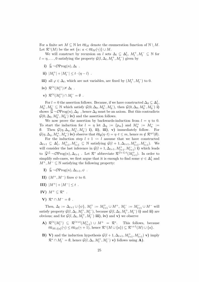
For a finite set M ⊆ N let enM denote the enumeration function of N \M .Let Rγ(M) be the set a : a < enM (γ) ∪M .

We will construct by recursion on l sets ∆l ⊆ .∆t1, M

+l ,M

−l ⊆ N for

l = η, . . . , 0 satisfying the property G(l,∆l,M+l ,M

−l ) given by

i) l• ¬OProg(n),∆l .

ii) |M+l |+ |M−

l | ≤ t · (η − l) .

iii) all ϕ ∈ ∆l, which are not variables, are fixed by (M+l ,M

−l ) to 0.

iv) Rl·t(M+l ) 2 ∆l .

v) Rl·t(M+l ) ∩M−

l = ∅ .

For l = 0 the assertion follows. Because, if we have constructed ∆0 ⊆ .∆t1,

M+0 ,M

−0 ⊆ N which satisfy G(0,∆0,M

+0 ,M

−0 ), then G(0,∆0,M

+0 ,M

−0 ) i)

shows 0• ¬OProg(n),∆0 , hence ∆0 must be an axiom. But this contradicts

G(0,∆0,M+0 ,M

−0 ) iv) and the assertion follows.

We now prove the assertion by backwards-induction from l = η to 0.To start the induction for l = η let ∆η := pm and M+

η := M−η :=

∅. Then G(η,∆η,M+η ,M

−η ) i), ii), iii), v) immediately follow. For

G(η,∆η,M+η ,M

−η ) iv) observe that en∅(η · t) = η · t ≤ m, hence m /∈ Rη·t(∅).

For the induction step l + 1 Ã l assume that we have constructed∆l+1 ⊆ .∆t

1, M+l+1,M

−l+1 ⊆ N satisfying G(l + 1,∆l+1,M

+l+1,M

−l+1). We

will consider the last inference in G(l + 1,∆l+1,M+l+1,M

−l+1) i) which leads

to l+1• ¬OProg(n),∆l+1 . Let R∗ abbreviate R(l+1)·t(M+

l+1). In order to

simplify sub-cases, we first argue that it is enough to find some ψ ∈ .∆t1 and

M+,M− ⊆ N satisfying the following property:

I) l• ¬OProg(n),∆l+1, ψ .

II) (M+,M−) fixes ψ to 0.

III) |M+|+ |M−| ≤ t .

IV) M+ ⊆ R∗ .

V) R∗ ∩M− = ∅ .

Then, ∆l := ∆l+1 ∪ ψ, M+l := M+

l+1 ∪M+, M−l := M−

l+1 ∪M− will

satisfy property G(l,∆l,M+l ,M

−l ), because G(l,∆l,M

+l ,M

−l ) i) and ii) are

obvious; and for G(l,∆l,M+l ,M

−l ) iii), iv) and v) we observe

A) Rl·t(M+l ) ⊆ Rl·t+t(M+

l+1) ∪ M+ = R∗. This follows, becauseenM∪a(γ) ≤ enM (γ + 1), hence Rγ(M ∪ a) ⊆ Rγ+1(M) ∪ a.

B) V) and the induction hypothesis G(l + 1,∆l+1,M+l+1,M

−l+1) v) imply

R∗ ∩M−l = ∅, hence G(l,∆l,M

+l ,M

−l ) v) follows using A).

25

C) A) and B) show ∅ 6= [M+l ,M

−l ]. By construction [M+

l ,M−l ] ⊆

[M+l+1,M

−l+1], hence (M+

l ,M−l ) fixes all ϕ ∈ ∆l+1 which are not vari-

ables, to 0.

Furthermore, [M+l ,M

−l ] ⊆ [M+,M−], hence II) implies that ψ is fixed

to 0 by (M+l ,M

−l ). Thus, G(l,∆l,M

+l ,M

−l ) iii) follows.

D) Utilising B) and A) we obtain Rl·t(M+l ),R∗ ∈ [M+

l ,M−l ] hence

G(l + 1,∆l+1,M+l+1,M

−l+1) iv) shows that (M+

l ,M−l ) fixes every for-

mula in ∆l+1 to 0. In particular, Rl·t(M+l ) 2 ∆l+1, which shows

G(l,∆l,M+l ,M

−l ) iv).

Now we distinguish sub-cases according to the last inference which leadsto l+1

• ¬OProg(n),∆l+1 . In the sub-cases, we either construct ψ, M+,M− satisfying I) to V), or we directly construct ∆l, M

+l , M−

l satisfyingG(l,∆l,M

+l ,M

−l ), depending which is easier.

(∧

) There is some ϕ =∧

j<J ϕj ∈ ∆l+1 such that l• ¬OProg(n),∆l+1, ϕj

for all j < J . By induction hypothesis G(l + 1,∆l+1,M+l+1,M

−l+1) iv)

we have that R∗ 2 ϕ. Thus, there is some j0 < J such that R∗ 2 ϕj0 .

Let ψ := ϕj0 , then ψ ∈ .∆t1 [⇒ I)]. By Lemma 28 there are some

M+ ⊆ R∗ [⇒ IV)] and M− ⊆ N such that R∗ ∩M− = ∅ [⇒ V)],|M+|+ |M−| ≤ t [⇒ III)] and (M+,M−) fixes ψ to 0 [⇒ II)].

(∨

) The first sub case is that ¬OInd(n) is not the main formula of theinference. Then, there is some ϕ =

∨

j<J ϕJ ∈ ∆l+1 such thatl• ¬OProg(n),∆l+1, ϕj0 for some j0 < J . By induction hypothesisG(l+1,∆l+1,M

+l+1,M

−l+1) iv) we have thatR∗ 2 ϕ, thus alsoR∗ 2 ϕj0 .

Now the same argumentation as in the∧

-case can be applied.

Now assume that the main formula is ¬OInd(n). Then, there is somex < n such that

l• ¬OProg(n),∆l+1,

(

∧

y<xpy

)

∧ ¬px .

A) Assume, there is some y < x such that y /∈ Rl·t(M+l+1).

By∧

-Inversion we obtain l• ¬OProg(n),∆l+1, py. Let ∆l :=

∆l+1, py [⇒ G(l,∆l,M+l ,M

−l ) i)], M+

l := M+l+1 and M−

l :=

M−l+1 [⇒ G(l,∆l,M

+l ,M

−l ) ii), iii)]. Now Rl·t(M+

l ) ⊆ R∗

[⇒ G(l,∆l,M+l ,M

−l ) v)], hence, using the assumption y /∈

Rl·t(M+l ), we obtain Rl·t(M+

l ) 2 ∆l [⇒ G(l,∆l,M+l ,M

−l ) iv)].

B) Now assume that A) does not hold, hence y ∈ Rl·t(M+l+1) for all

y < x. This implies x ∈ Rl·t+1(M+l+1) ⊆ R∗. Because, enM (γ) /∈

Rγ(M), hence y ∈ Rγ(M) for all y < x implies enM (γ) ≥ x,hence enM (γ + 1) > x and in sequel x ∈ Rγ+1(M).

26

By∧

-Inversion we obtain l• ¬OProg(n),∆l+1,¬px. Let ψ :=

¬px [⇒ I)], M+ := x and M− := ∅ [⇒ II), III), IV), V)].

(Cut) There is some ϕ ∈ .∆t1 such that l

• ¬OProg(n),∆l+1, ϕ andl• ¬OProg(n),∆l+1,¬ϕ. W.l.o.g. we may assume R∗ 2 ϕ. The same

argumentation as in the∧

-case yields the assertion.

8 Generalised dynamic ordinals revisited

We have now collected all tools which are needed to compute the missingupper bounds on generalised dynamic ordinals. Our strategy will be totranslate a Σb

m+i(α)-LmIND-proof of OInd(t(x),Πbi) to Σqp

i -LK, and thenuse the result on lower bounds of the order induction principle, Theorem 26,to obtain tight upper bounds on generalised dynamic ordinals.

For the following considerations fix some i,m ∈ N with m > 0 and some

f ∈ DOi+1(Σbm+i(α)-LmIND) .

First, we define some general Πbi(α)-formula Aα,i(a, x), which is trans-

lated by the Paris-Wilkie translation to the Sipser function Di,a as definedbefore. Aα,i(a, x) is given by the formula

(∀y1 < a) (∃y2 < a) . . . (Qi−1yi−1 < a) (Qiyi < a) α(〈x, y1, . . . , yi〉)

where either Qi−1 or Qi is ∀, depending on whether i is even or odd, respec-tively, and the other is ∃. Here, 〈z1, . . . , zj〉 denotes some sequence codingfunction expressible in the language of bounded arithmetic. Then, the def-inition of DOi+1 yields that there is some term t such that f = λx.t(x)and

Σbm+i(α)-LmIND ` (∀x)OInd(t,¬Aα,i(t, .)) .

Utilising Theorem 19 shows that there is some c ≥ 1 such that eventually

[[OInd(t(n),¬Aα,i(t(n), .))]]

is Σqpi -LK provable with height 2m−1

(

(log(m) n)c)

. By identifying p〈x,~y〉

with px,~y, we see that these derivations transform to Σqpi -LK proofs of

OInd(t(n))[

px ← ¬Di,t(n)(x) : x < t(n)]

of height 2m−1

(

(log(m) n)c)

.

27

Now we are in the situation that we can apply the Lower Bound Theo-

rem 26, because 2m−1

(

(log(m) n)c)

= (log n)Ω(1). Hence, we obtain that

f(n) = t(n) = 2m−1

(

(log(m) n)c)O(1)

= 2m(O(log(m+1) n)) .

Together with Corollary 8, this shows:

Theorem 30. Let m > 0. The i + 1 generalised dynamic ordinal of thetheory Σb

m+i(α)-LmIND can be described as:

DOi+1(Σbm+i(α)-LmInd) ≡ 2m(O(| id |m+1)) .

Hence we have for i > 0:

DOi(Ti2(α)) ≡ 22(O(| id |2)) ≡ DOi(S

i+12 (α))

DOi(Si2(α)) ≡ 21(O(| id |2))

DOi(sRi+12 (α)) ≡ 22(O(| id |3))

We also compare definable multivalued functions of unrelativised theorieswith the generalised dynamic ordinals of their relativised companions.

Theorem 31. Let i ≥ 0. For any theory T from the infinite list

Ti+12 , Si+2

2 , Si+12 , sRi+2

2 (= Σbi+2-L

2IND), Σbi+3-L

3IND, . . .

we have:

A multivalued function f is Σbi+2-definable in T , if and only if

f ∈ FPΣbi+1(wit, log(DOi+1(T (α)))).

This indicates that generalised dynamic ordinals do in fact also charac-terise the computational complexity of bounded arithmetic theories.

References

[1] Theodore Baker, John Gill, and Robert Solovay. Relativizations of theP =?NP question. SIAM J. Comput., 4(4):431–442, 1975.

[2] Arnold Beckmann. Seperating fragments of bounded predicative arith-metic. PhD thesis, Westfalische Wilhelms-Universitat, Munster, 1996.

[3] Arnold Beckmann. A note on universal measures for weak implicitcomputational complexity. In Matthias Baaz and Andrei Voronkov,editors, Proccedings of the 9th International Conference, LPAR 2002(Tbilisi), Lecture Notes in Computer Science, pages 53–67, Berlin, 2002.Springer-Verlag.

28

[4] Arnold Beckmann. Dynamic ordinal analysis. Arch. Math. Logic,42:303–334, 2003.

[5] Arnold Beckmann. Height restricted constant depth LK. Research NoteReport TR03-034, Electronic Colloquium on Computational Complex-ity, 2003. http://www.eccc.uni-trier.de/eccc-reports/2003/TR03-034/.

[6] Samuel R. Buss. Bounded arithmetic, volume 3 of Stud. Proof Theory,Lect. Notes. Bibliopolis, Naples, 1986.

[7] Samuel R. Buss. Axiomatizations and conservation results for fragmentsof bounded arithmetic. In Wilfried Sieg, editor, Proceedings of theworkshop held at Carnegie Mellon University, Pittsburgh, Pennsylvania,June 30–July 2, 1987, volume 106 of Contemporary Mathematics, pages57–84, Providence, RI, 1990. American Mathematical Society.

[8] Samuel R. Buss. Relating the bounded arithmetic and the polynomialtime hierarchies. Ann. Pure Appl. Logic, 75:67–77, 1995.

[9] Samuel R. Buss and Jan Krajıcek. An application of boolean complexityto separation problems in bounded arithmetic. Proc. London Math.Soc., 69:1–21, 1994.

[10] Johan Hastad. Computational Limitations of Small Depth Circuits.MIT Press, Cambridge, MA, 1987.

[11] Johan Hastad. Almost optimal lower bounds for small depth circuits.Randomness and Computation, 5:143–70, 1989.

[12] Jan Johannsen. A note on sharply bounded arithmetic. Arch. Math.Logik Grundlag., 33:159–165, 1994.

[13] Jan Krajıcek. Fragments of bounded arithmetic and bounded queryclasses. Trans. Amer. Math. Soc., 338:587–98, 1993.

[14] Jan Krajıcek. Lower bounds to the size of constant-depth propositionalproofs. J. Symbolic Logic, 59:73–86, 1994.

[15] Jan Krajıcek. Bounded Arithmetic, Propositional Logic, and Complex-ity Theory. Cambridge University Press, Heidelberg/New York, 1995.

[16] Jan Krajıcek, Pavel Pudlak, and Gaisi Takeuti. Bounded arithmetic andthe polynomial hierarchy. Ann. Pure Appl. Logic, 52:143–153, 1991.

[17] Daniel Leivant. Substructural termination proofs and feasibility certifi-cation. In Proceedings of the 3rd Workshop on Implicit ComputationalComplexity (Aarhus), pages 75–91, 2001.

29

[18] Jeff B. Paris and Alex J. Wilkie. Counting problems in bounded arith-metic. In Carlos Augusto di Prisco, editor, Methods in Mathemati-cal Logic, number 1130 in Lect. Notes Math., pages 317–340, Heidel-berg/New York, August 1985. Springer.

[19] Wolfram Pohlers. Proof theory, volume 1407 of Lecture Notes in Math-ematics. Springer-Verlag, Berlin, 1989. An introduction.

[20] Chris Pollett. Structure and definability in general bounded arithmetictheories. Ann. Pure Appl. Logic, 100(1-3):189–245, 1999.

[21] Gaisi Takeuti. RSUV isomorphism. In Peter Clote and Jan Krajıcek,editors, Arithmetic, proof theory, and computational complexity, OxfordLogic Guides, pages 364–86. Oxford University Press, New York, 1993.

[22] Andrew C. Yao. Separating the polynomial-time hierarchy by oracles.Proc. 26th Ann. IEEE Symp. on Foundations of Computer Science,pages 1–10, 1985.

[23] Domenico Zambella. Notes on polynomially bounded arithmetic. J.Symbolic Logic, 61:942–966, 1996.

30