
Generalised interval-valued fuzzy soft set
19
Hindawi Publishing Corporation Journal of Applied Mathematics Volume 2012, Article ID 870504, 18 pages doi:10.1155/2012/870504 Research Article Generalised Interval-Valued Fuzzy Soft Set Shawkat Alkhazaleh and Abdul Razak Salleh School of Mathematical Sciences, Faculty of Science and Technology, Universiti Kebangsaan Malaysia, 43600 UKM Bangi, Selangor, Malaysia Correspondence should be addressed to Shawkat Alkhazaleh, [email protected] Received 6 August 2011; Revised 21 January 2012; Accepted 22 February 2012 Academic Editor: Ch. Tsitouras Copyright q 2012 S. Alkhazaleh and A. R. Salleh. This is an open access article distributed under the Creative Commons Attribution License, which permits unrestricted use, distribution, and reproduction in any medium, provided the original work is properly cited. We introduce the concept of generalised interval-valued fuzzy soft set and its operations and study some of their properties. We give applications of this theory in solving a decision making problem. We also introduce a similarity measure of two generalised interval-valued fuzzy soft sets and discuss its application in a medical diagnosis problem: fuzzy set; soft set; fuzzy soft set; generalised fuzzy soft set; generalised interval-valued fuzzy soft set; interval-valued fuzzy set; interval-valued fuzzy soft set. 1. Introduction Molodtsov 1 initiated the theory of soft set as a new mathematical tool for dealing with uncertainties which traditional mathematical tools cannot handle. He has shown several applications of this theory in solving many practical problems in economics, engineering, social science, medical science, and so forth. Presently, work on the soft set theory is progress- ing rapidly. Maji et al. 2, 3, Roy and Maji 4 have further studied the theory of soft set and used this theory to solve some decision making problems. Maji et al. 5 have also introduced the concept of fuzzy soft set, a more general concept, which is a combination of fuzzy set and soft set and studied its properties. Zou and Xiao 6 introduced soft set and fuzzy soft set into the incomplete environment, respectively. Alkhazaleh et al. 7 introduced the concept of soft multiset as a generalisation of soft set. They also defined the concepts of fuzzy parameterized interval-valued fuzzy soft set 8 and possibility fuzzy soft set 9 and gave their applications in decision making and medical diagnosis. Alkhazaleh and Salleh 10 introduced the concept of a soft expert set, where the user can know the opinion of all experts in one model without any operations. Even after any operation, the user can know the opinion of all experts. In 2011, Salleh 11 gave a brief survey from soft set to intuitionistic fuzzy soft set. Majumdar and Samanta 12 introduced and studied generalised fuzzy soft set where the degree is
Transcript of Generalised interval-valued fuzzy soft set

Hindawi Publishing CorporationJournal of Applied MathematicsVolume 2012, Article ID 870504, 18 pagesdoi:10.1155/2012/870504
Research ArticleGeneralised Interval-Valued Fuzzy Soft Set
Shawkat Alkhazaleh and Abdul Razak Salleh
School of Mathematical Sciences, Faculty of Science and Technology, Universiti Kebangsaan Malaysia,43600 UKM Bangi, Selangor, Malaysia
Correspondence should be addressed to Shawkat Alkhazaleh, [email protected]
Received 6 August 2011; Revised 21 January 2012; Accepted 22 February 2012
Academic Editor: Ch. Tsitouras
Copyright q 2012 S. Alkhazaleh and A. R. Salleh. This is an open access article distributed underthe Creative Commons Attribution License, which permits unrestricted use, distribution, andreproduction in any medium, provided the original work is properly cited.
We introduce the concept of generalised interval-valued fuzzy soft set and its operations and studysome of their properties. We give applications of this theory in solving a decision making problem.We also introduce a similarity measure of two generalised interval-valued fuzzy soft sets anddiscuss its application in amedical diagnosis problem: fuzzy set; soft set; fuzzy soft set; generalisedfuzzy soft set; generalised interval-valued fuzzy soft set; interval-valued fuzzy set; interval-valuedfuzzy soft set.
1. Introduction
Molodtsov [1] initiated the theory of soft set as a new mathematical tool for dealing withuncertainties which traditional mathematical tools cannot handle. He has shown severalapplications of this theory in solving many practical problems in economics, engineering,social science, medical science, and so forth. Presently, work on the soft set theory is progress-ing rapidly. Maji et al. [2, 3], Roy and Maji [4] have further studied the theory of soft set andused this theory to solve some decision making problems. Maji et al. [5] have also introducedthe concept of fuzzy soft set, a more general concept, which is a combination of fuzzy set andsoft set and studied its properties. Zou and Xiao [6] introduced soft set and fuzzy soft set intothe incomplete environment, respectively. Alkhazaleh et al. [7] introduced the concept of softmultiset as a generalisation of soft set. They also defined the concepts of fuzzy parameterizedinterval-valued fuzzy soft set [8] and possibility fuzzy soft set [9] and gave their applicationsin decisionmaking andmedical diagnosis. Alkhazaleh and Salleh [10] introduced the conceptof a soft expert set, where the user can know the opinion of all experts in one model withoutany operations. Even after any operation, the user can know the opinion of all experts. In2011, Salleh [11] gave a brief survey from soft set to intuitionistic fuzzy soft set. Majumdarand Samanta [12] introduced and studied generalised fuzzy soft set where the degree is

2 Journal of Applied Mathematics
attached with the parameterization of fuzzy sets while defining a fuzzy soft set. Yang et al.[13] presented the concept of interval-valued fuzzy soft set by combining the interval-valuedfuzzy set [14, 15] and soft set models. In this paper, we generalise the concept of fuzzysoft set as introduced by Maji et al. [5] to generalised interval-valued fuzzy soft set. In ourgeneralisation of fuzzy soft set, a degree is attached with the parameterization of fuzzysets while defining an interval-valued fuzzy soft set. Also, we give some applications ofgeneralised interval-valued fuzzy soft set in decisionmaking problem andmedical diagnosis.
2. Preliminary
In this section, we recall some definitions and properties regarding fuzzy soft set andgeneralised fuzzy soft set required in this paper.
Definition 2.1 (see [15]). An interval-valued fuzzy set ˜X on a universe U is a mapping suchthat
˜X : U −→ Int([0, 1]), (2.1)
where Int([0, 1]) stands for the set of all closed subintervals of [0, 1], the set of all interval-valued fuzzy sets on U is denoted by ˜P(U).
Suppose that ˜X ∈ ˜P(U), for all x ∈ U, μx(x) = [μ−x(x), μ
+x(x)] is called the degree of
membership of an element x to X. μ−x(x) and μ+
x(x) are referred to as the lower and upperdegrees of membership of x to X where 0 � μ−
x(x) � μ+x(x) � 1.
Definition 2.2 (see [14]). The subset, complement, intersection, and union of the interval-valued fuzzy sets are defined as follows. Let ˜X, ˜Y ∈ ˜P(U), then
(a) the complement of ˜X is denoted by ˜Xc where
μ˜Xc(x) = 1 − μ
˜X(x) =[
1 − μ+˜X(x), 1 − μ−
˜X(x)
]
, (2.2)
(b) the intersection of ˜X and ˜Y is denoted by ˜X ∩ ˜Y where
μ˜X∩ ˜Y (x) = inf
[
μ˜X(x), μ ˜Y (x)
]
=[
inf(
μ−˜X(x), μ−
˜Y(x)
)
, inf(
μ+˜X(x), μ+
˜Y(x)
)]
,(2.3)
(c) the union of ˜X and ˜Y is denoted by ˜X ∪ ˜Y where
μ˜X∪ ˜Y (x) = sup
[
μ˜X(x), μ ˜Y (x)
]
=[
sup(
μ−˜X(x), μ−
˜Y(x)
)
, sup(
μ+˜X(x), μ+
˜Y(x)
)]
;(2.4)
(d) X is a subset of Ydenoted by X ⊆ Y if μ−X(x) ≤ μ−
Y (x) and μ+X(x) ≤ μ+
Y (x).

Journal of Applied Mathematics 3
Definition 2.3 (see [14]). The compatibility measure ϕ(A,B) of an interval-valued fuzzy setAwith an interval-valued fuzzy set B (A is a reference set) is given by
ϕ(A,B) =[
ϕ−(A,B), ϕ+(A,B)]
, (2.5)
such that
ϕ−(A,B) = min[
ϕ1(A,B), ϕ2(A,B)]
,
ϕ+(A,B) = max[
ϕ1(A,B), ϕ2(A,B)]
,(2.6)
where
ϕ1(A,B) =maxx∈X
{
min[
μ−A(x), μ
−B(x)
]}
maxx∈X[
μ−A(x)
] ,
ϕ2(A,B) =maxx∈X
{
min[
μ+A(x), μ
+B(x)
]}
maxx∈X[
μ+A(x)
] .
(2.7)
Theorem 2.4 (see [14]). Consider arbitrary, nonempty interval-valued fuzzy sets A, B, and C fromthe family of ivf(X) and a compatibility measure in the sense of Definition 2.3. Then,
(a) A ϕ(A,A) = [1, 1] = {1},
(b) ϕ(A,B) = [0, 0] = {0} ⇔ A ∩ B = ∅,
(c) in general ϕ(A,B)/= ϕ(B,A).
LetU be a universal set and E a set of parameters. Let P(U) denote the power set ofUand A ⊆ E. Molodtsov [1] defined soft set as follows.
Definition 2.5. A pair (F, E) is called a soft set overU, where F is a mapping given by F : E →P(U). In other words, a soft set over U is a parameterized family of subsets of the universeU.
Definition 2.6 (see [5]). LetU be a universal set, and let E be a set of parameters. Let IU denotethe power set of all fuzzy subsets of U. Let A ⊆ E. A pair (F, E) is called a fuzzy soft set overU where F is a mapping given by
F : A −→ IU. (2.8)
Definition 2.7 (see [12]). Let U = {x1, x2, . . . , xn} be the universal set of elements and E ={e1, e2, . . . , em} be the universal set of parameters. The pair (U,E)will be called a soft universe.

4 Journal of Applied Mathematics
Let F : E → IU, where IU is the collection of all fuzzy subsets ofU, and let μ be a fuzzy subsetof E. Let Fμ : E → IU × I be a function defined as follows:
Fμ(e) =(
F(e), μ(e))
. (2.9)
Then, Fμ is called a generalised fuzzy soft set (GFSS in short) over the soft set (U,E). Here,for each parameter ei, Fμ(ei) = (F(ei), μ(ei)) indicates not only the degree of belongingnessof the elements of U in F(ei) but also the degree of possibility of such belongingness whichis represented by μ(ei). So we can write Fμ(ei) as follows:
Fμ(ei) =({
x1
F(ei)(x1),
x2
F(ei)(x2), . . . ,
xn
F(ei)(xn)
}
, μ(ei))
, (2.10)
where F(ei)(x1), F(ei)(x2), . . . , F(ei)(xn) are the degree of belongingness and μ(ei) is thedegree of possibility of such belongingness.
Definition 2.8 (see [13]). LetU be an initial universe and E a set of parameters. ˜P(U) denotesthe set of all interval-valued fuzzy sets of U. Let A ⊆ E. A pair ( ˜F,A) is an interval-valuedfuzzy soft set over U, where ˜F is a mapping given by ˜F : A → ˜P(U).
3. Generalised Interval-Valued Fuzzy Soft Set
In this section, we generalise the concept of interval-valued fuzzy soft sets as introduced in[13]. In our generalisation of interval-valued fuzzy soft set, a degree is attached with theparameterization of fuzzy sets while defining an interval-valued fuzzy soft set.
Definition 3.1. LetU = {x1, x2, . . . , xn} be the universal set of elements and E = {e1, e2, . . . , em}the universal set of parameters. The pair (U,E) will be called a soft universe. Let ˜F : E →˜P(U) and μ be a fuzzy set of E, that is, μ : E → I = [0, 1], where ˜P(U) is the set of allinterval-valued fuzzy subsets onU. Let ˜Fμ : E → ˜P(U) × I be a function defined as follows:
˜Fμ(e) =(
˜F(e), μ(e))
. (3.1)
Then, ˜Fμ is called a generalised interval-valued fuzzy soft set (GIVFSS in short) over thesoft universe (U,E). For each parameter ei, ˜Fμ(ei) = ( ˜F(ei)(x), μ(ei)) indicates not only thedegree of belongingness of the elements of U in ˜F(ei) but also the degree of possibility ofsuch belongingness which is represented by μ(ei). So we can write ˜Fμ(ei) as follows:
˜Fμ(ei) =
({
x1
˜F(ei)(x1),
x2
˜F(ei)(x2), . . . ,
xn
˜F(ei)(xn)
}
, μ(ei)
)
. (3.2)

Journal of Applied Mathematics 5
Example 3.2. Let U = {x1, x2, x3} be a set of universe, E = {e1, e2, e3} a set of parameters, andlet μ : E → I. Define a function ˜Fμ : E → ˜P(U) × I as follows:
˜Fμ(e1) =({
x1
[0.3, 0.6],
x2
[0.7, 0.8],
x3
[0.5, 0.8]
}
, 0.6)
,
˜Fμ(e2) =({
x1
[0.1, 0.4],
x2
[0, 0.3],
x3
[0.1, 0.5]
}
, 0.5)
,
˜Fμ(e3) =({
x1
[0.7, 0.8],
x2
[0.1, 0.2],
x3
[0, 0.4]
}
, 0.3)
.
(3.3)
Then, ˜Fμ is a GIVFSS over (U,E).In matrix notation, we write
˜Fμ =
⎛
⎝
[0.3, 0.6] [0.7, 0.8] [0.5, 0.8] 0.6[0.1, 0.4] [0, 0.3] [0.1, 0.5] 0.5[0.7, 0.8] [0.1, 0.2] [0, 0.4] 0.3
⎞
⎠. (3.4)
Definition 3.3. Let ˜Fμ and ˜Gδ be two GIVFSSs over (U,E). ˜Fμ is called a generalised interval-valued fuzzy soft subset of ˜Gδ, and we write ˜Fμ ⊆ ˜Gδ if
(a) μ(e) is a fuzzy subset of δ(e) for all e ∈ E,
(b) ˜F(e) is an interval-valued fuzzy subset of ˜G(e) for all e ∈ E.
Example 3.4. Let U = {x1, x2, x3} be a set of three cars, and let E = {e1, e2, e3} be a set ofparameters where e1 = cheap, e2 = expensive, e3 = red. Let ˜Fμ be a GIVFSS over (U,E) definedas follows:
˜Fμ(e1) =({
x1
[0.1, 0.3],
x2
[0.5, 0.7],
x3
[0.3, 0.5]
}
, 0.4)
,
˜Fμ(e2) =({
x1
[0, 0.3],
x2
[0, 0.2],
x3
[0.1, 0.3]
}
, 0.4)
,
˜Fμ(e3) =({
x1
[0.5, 0.6],
x2
[0.1, 0.1],
x3
[0.1, 0.3]
}
, 0.1)
.
(3.5)
Let ˜Gδ be another GIVFSS over (U,E) defined as follows:
˜Gδ(e1) =({
x1
[0.3, 0.6],
x2
[0.7, 0.8],
x3
[0.5, 0.8]
}
, 0.6)
,
˜Gδ(e2) =({
x1
[0.2, 0.4],
x2
[0.2, 0.3],
x3
[0.3, 0.5]
}
, 0.5)
,
˜Gδ(e3) =({
x1
[0.7, 0.8],
x2
[0.2, 0.4],
x3
[0.2, 0.5]
}
, 0.3)
.
(3.6)
It is clear that ˜Fμ is a GIVFS subset of ˜Gδ.

6 Journal of Applied Mathematics
Definition 3.5. Two GIVFSSs ˜Fμ and ˜Gδ over (U,E) are said to be equal, and we write ˜Fμ = ˜Gδ
if ˜Fμ is a GIVFS subset of ˜Gδ and ˜Gδ is a GIVFS subset of ˜Fμ. In other words, ˜Fμ = ˜Gδ if thefollowing conditions are satisfied:
(a) μ(e) is equal to δ(e) for all e ∈ E,
(b) ˜F(e) is equal to ˜G(e) for all e ∈ E.
Definition 3.6. A GIVFSS is called a generalised null interval-valued fuzzy soft set, denotedby ˜∅μ if ˜∅μ : E → ˜P(U) × I such that
˜∅μ(e) =(
˜F(e)(x), μ(e))
, (3.7)
where ˜F(e) = [0, 0] = [0] and μ(e) = 0 for all e ∈ E.
Definition 3.7. A GIVFSS is called a generalised absolute interval-valued fuzzy soft set,denoted by ˜Aμ if ˜Aμ : E → ˜P(U) × I such that
˜Aμ(e) =(
˜F(e)(x), μ(e))
, (3.8)
where ˜F(e) = [1, 1] = [1], and μ(e) = 1 for all e ∈ E.
4. Basic Operations on GIVFSS
In this section, we introduce some basic operations on GIVFSS, namely, complement, unionand intersection and we give some properties related to these operations.
Definition 4.1. Let ˜Fμ be a GIVFSS over (U,E). Then, the complement of ˜Fμ, denoted by ˜Fcμ
and is defined by ˜Fcμ = ˜Gδ, such that δ(e) = c(μ(e)) and ˜G(e) = c̃( ˜F(e)) for all e ∈ E, where c
is a fuzzy complement and c̃ is an interval-valued fuzzy complement.
Example 4.2. Consider a GIVFSS ˜Fμ over (U,E) as in Example 3.2:
˜Fμ =
⎛
⎝
[0.3, 0.6] [0.7, 0.8] [0.5, 0.8] 0.6[0.1, 0.4] [0, 0.3] [0.1, 0.5] 0.5[0.7, 0.8] [0.1, 0.2] [0, 0.4] 0.3
⎞
⎠. (4.1)
By using the basic fuzzy complement for μ(e) and interval-valued fuzzy complement for˜F(e), we have ˜Fc
μ = Gδ where
Gδ =
⎛
⎝
[0.4, 0.7] [0.2, 0.3] [0.2, 0.5] 0.4[0.6, 0.9] [0.7, 1] [0.5, 0.9] 0.5[0.2, 0.3] [0.8, 0.9] [0.6, 1] 0.7
⎞
⎠. (4.2)

Journal of Applied Mathematics 7
Proposition 4.3. Let ˜Fμ be a GIVFSS over (U,E). Then, the following holds:
(
˜Fcμ
)c= ˜Fμ. (4.3)
Proof. Since ˜Fcμ = ˜Gδ, then
(
˜Fcμ
)c= ˜Gc
δ (4.4)
but, from Definition 4.1, ˜Gδ = (c̃( ˜F(e)), c(μ(e))), then
˜Gcδ =
(
c̃(
c̃(
˜F(e)))
, c(
c(
μ(e)))
)
=(
˜F(e), μ(e))
= ˜Fμ.
(4.5)
Definition 4.4. Union of two GIVFSSs ( ˜Fμ,A) and ( ˜Gδ, B), denoted by ˜Fμ ∪ ˜Gδ, is a GIVFSS(˜Hν,C)where C = A ∪ B and ˜Hν : E → ˜P(U) × I is defined by
˜Hν(e) =(
˜H(e), ν(e))
(4.6)
such that ˜H(e) = ˜F(e) ∪ ˜G(e) and ν(e) = s(μ(e), δ(e)), where s is an s-norm and ˜H(e) =[sup(μ−
˜F(e), μ−
˜G(e)), sup(μ+
˜F(e), μ+
˜G(e))].
Example 4.5. Consider GIVFSS ˜Fμ and ˜Gδ as in Example 3.4. By using the interval-valuedfuzzy union and basic fuzzy union, we have ˜Fμ ∪ ˜Gδ = ˜Hv, where
˜Hv(e1) =
({
x1[
sup(0.1, 0.3), sup(0.3, 0.6)] ,
x2[
sup(0.5, 0.7), sup(0.7, 0.8)] ,
x3[
sup(0.3, 0.5), sup(0.5, 0.8)]
}
,max(0.4, 0.6)
)
=({
x1
[0.3, 0.6],
x2
[0.7, 0.8],
x3
[0.5, 0.8]
}
, 0.6)
.
(4.7)
Similarly, we get
˜Hv(e2) =({
x1
[0.2, 0.4],
x2
[0.2, 0.3],
x3
[0.3, 0.5]
}
, 0.5)
,
˜Hv(e3) =({
x1
[0.7, 0.8],
x2
[0.2, 0.4],
x3
[0.2, 0.5]
}
, 0.3)
.
(4.8)
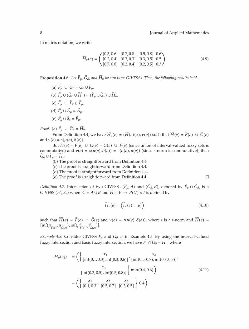
8 Journal of Applied Mathematics
In matrix notation, we write
˜Hv(e) =
⎛
⎝
[0.3, 0.6] [0.7, 0.8] [0.5, 0.8] 0.6[0.2, 0.4] [0.2, 0.3] [0.3, 0.5] 0.5[0.7, 0.8] [0.2, 0.4] [0.2, 0.5] 0.3
⎞
⎠. (4.9)
Proposition 4.6. Let ˜Fμ, ˜Gδ, and ˜Hv be any three GIVFSSs. Then, the following results hold.
(a) ˜Fμ ∪ ˜Gδ = ˜Gδ ∪ ˜Fμ.
(b) ˜Fμ ∪ ( ˜Gδ ∪ ˜Hv) = ( ˜Fμ ∪ ˜Gδ) ∪ ˜Hv.
(c) ˜Fμ ∪ ˜Fμ ⊆ ˜Fμ.
(d) ˜Fμ ∪ ˜Aμ = ˜Aμ.
(e) ˜Fμ ∪ ˜∅μ = ˜Fμ.
Proof. (a) ˜Fμ ∪ ˜Gδ = ˜Hν.From Definition 4.4, we have ˜Hν(e) = (˜H(e)(x), ν(e)) such that ˜H(e) = ˜F(e) ∪ ˜G(e)
and ν(e) = s(μ(e), δ(e)).But ˜H(e) = ˜F(e) ∪ ˜G(e) = ˜G(e) ∪ ˜F(e) (since union of interval-valued fuzzy sets is
commutative) and ν(e) = s(μ(e), δ(e)) = s(δ(e), μ(e)) (since s-norm is commutative), then˜Gδ ∪ ˜Fμ = ˜Hν.
(b) The proof is straightforward from Definition 4.4.(c) The proof is straightforward from Definition 4.4.(d) The proof is straightforward from Definition 4.4.(e) The proof is straightforward from Definition 4.4.
Definition 4.7. Intersection of two GIVFSSs ( ˜Fμ,A) and ( ˜Gδ, B), denoted by ˜Fμ ∩ ˜Gδ, is aGIVFSS (˜Hν,C) where C = A ∪ B and ˜Hν : E → ˜P(U) × I is defined by
˜Hν(e) =(
˜H(e), ν(e))
(4.10)
such that ˜H(e) = ˜F(e) ∩ ˜G(e) and ν(e) = t(μ(e), δ(e)), where t is a t-norm and ˜H(e) =[inf(μ−
˜F(e), μ−
˜G(e)), inf(μ+
˜F(e), μ+
˜G(e))].
Example 4.8. Consider GIVFSS ˜Fμ and ˜Gδ as in Example 4.5. By using the interval-valuedfuzzy intersection and basic fuzzy intersection, we have ˜Fμ ∩ ˜Gδ = ˜Hv, where
˜Hv(e1) =({
x1
[inf(0.1, 0.3), inf(0.3, 0.6)],
x2
[inf(0.5, 0.7), inf(0.7, 0.8)],
x3
[inf(0.3, 0.5), inf(0.5, 0.8)]
}
min(0.4, 0.6))
=({
x1
[0.1, 0.3],
x2
[0.5, 0.7],
x3
[0.3, 0.5]
}
, 0.4)
.
(4.11)

Journal of Applied Mathematics 9
Similarly, we get
˜Hv(e2) =({
x1
[0, 0.3],
x2
[0, 0.2],
x3
[0.1, 0.3]
}
, 0.4)
,
˜Hv(e3) =({
x1
[0.5, 0.6],
x2
[0.1, 0.1],
x3
[0.1, 0.3]
}
, 0.1)
.
(4.12)
In matrix notation, we write
˜Hv(e) =
⎛
⎝
[0.1, 0.3] [0.5, 0.7] [0.3, 0.5] 0.4[0, 0.3] [0, 0.2] [0.1, 0.3] 0.4[0.5, 0.6] [0.1, 0.1] [0.1, 0.3] 0.1
⎞
⎠. (4.13)
Proposition 4.9. Let ˜Fμ, ˜Gδ, and ˜Hv be any three GIVFSSs. Then, the following results hold.
(a) ˜Fμ ∩ ˜Gδ = ˜Gδ ∩ ˜Fμ.
(b) ˜Fμ ∩ ( ˜Gδ ∩ ˜Hv) = ( ˜Fμ ∩ ˜Gδ) ∩ ˜Hv.
(c) ˜Fμ ∩ ˜Fμ ⊆ ˜Fμ.
(d) ˜Fμ ∩ ˜Aμ = ˜Fμ.
(e) ˜Fμ ∩ ˜∅μ = ˜∅μ.
Proof. (a) ˜Fμ ∩ ˜Gδ = ˜Hν.From Definition 4.7, we have ˜Hν(e) = (˜H(e)(x), ν(e)) such that ˜H(e) = ˜F(e) ∩ ˜G(e)
and ν(e) = t(μ(e), δ(e)).But ˜H(e) = ˜F(e) ∩ ˜G(e) = ˜G(e) ∩ ˜F(e) (since intersection of interval-valued fuzzy
sets is commutative) and ν(e) = t(μ(e), δ(e)) = t(δ(e), μ(e)) (since t-norm is commutative),then ˜Gδ ∩ ˜Fμ = ˜Hν.
(b) The proof is straightforward from Definition 4.7.(c) The proof is straightforward from Definition 4.7.(d) The proof is straightforward from Definition 4.7.(e) The proof is straightforward from Definition 4.7.
Proposition 4.10. Let ˜Fμ and ˜Gδ be any two GIVFSSs. Then the DeMorgan’s Laws hold:
(a) ( ˜Fμ ∪ ˜Gδ)c= ˜Gc
δ ∩ ˜Fcμ.
(b) ( ˜Fμ ∩ ˜Gδ)c= ˜Gc
δ∪ ˜Fc
μ.
Proof. (a) Consider
˜Fcμ ∩ ˜Gc
δ =((
c̃(F(e)), c(
μ(e))) ∩ (c̃(G(e)), c(δ(e)))
)
=(
(c̃(F(e)) ∩ c̃(G(e))),(
c(
μ(e)) ∩ c(δ(e))
))
=(
((F(e)) ∪ (G(e)))c̃,(
μ(e) ∪ δ(e))c)
=(
˜Fμ ∪ ˜Gδ
)c.
(4.14)
(b) The proof is similar to the above.
10 Journal of Applied Mathematics
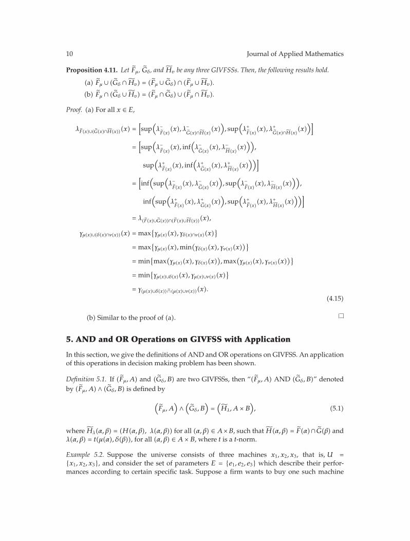
Proposition 4.11. Let ˜Fμ, ˜Gδ, and ˜Hv be any three GIVFSSs. Then, the following results hold.
(a) ˜Fμ ∪ ( ˜Gδ ∩ ˜Hv) = ( ˜Fμ ∪ ˜Gδ) ∩ ( ˜Fμ ∪ ˜Hv).
(b) ˜Fμ ∩ ( ˜Gδ ∪ ˜Hv) = ( ˜Fμ ∩ ˜Gδ) ∪ ( ˜Fμ ∩ ˜Hv).
Proof. (a) For all x ∈ E,
λ˜F(x)∪( ˜G(x)∩˜H(x))(x) =
[
sup(
λ−˜F(x)
(x), λ−˜G(x)∩˜H(x)
(x))
, sup(
λ+˜F(x)
(x), λ+˜G(x)∩˜H(x)
(x))]
=[
sup(
λ−˜F(x)
(x), inf(
λ−˜G(x)
(x), λ−˜H(x)
(x)))
,
sup(
λ+˜F(x)
(x), inf(
λ+˜G(x)
(x), λ+˜H(x)
(x)))]
=[
inf(
sup(
λ−˜F(x)
(x), λ−˜G(x)
(x))
, sup(
λ−˜F(x)
(x), λ−˜H(x)
(x)))
,
inf(
sup(
λ+˜F(x)
(x), λ+˜G(x)
(x))
, sup(
λ+˜F(x)
(x), λ+˜H(x)
(x)))]
= λ( ˜F(x)∪ ˜G(x))∩( ˜F(x)∪˜H(x))(x),
γμ(x)∪(δ(x)∩ν(x))(x) = max{
γμ(x)(x), γδ(x)∩ν(x)(x)}
= max{
γμ(x)(x),min(
γδ(x)(x), γν(x)(x))}
= min{
max(
γμ(x)(x), γδ(x)(x))
,max(
γμ(x)(x), γν(x)(x))}
= min{
γμ(x)∪δ(x)(x), γμ(x)∪ν(x)(x)}
= γ(μ(x)∪δ(x)) ˜∩ (μ(x)∪ν(x))(x).(4.15)
(b) Similar to the proof of (a).
5. AND and OR Operations on GIVFSS with Application
In this section, we give the definitions of AND and OR operations on GIVFSS. An applicationof this operations in decision making problem has been shown.
Definition 5.1. If ( ˜Fμ,A) and ( ˜Gδ, B) are two GIVFSSs, then “( ˜Fμ,A) AND ( ˜Gδ, B)” denotedby ( ˜Fμ,A) ∧ ( ˜Gδ, B) is defined by
(
˜Fμ,A)
∧(
˜Gδ, B)
=(
˜Hλ,A × B)
, (5.1)
where ˜Hλ(α, β) = (H(α, β), λ(α, β)) for all (α, β) ∈ A×B, such that ˜H(α, β) = ˜F(α)∩ ˜G(β) andλ(α, β) = t(μ(α), δ(β)), for all (α, β) ∈ A × B, where t is a t-norm.
Example 5.2. Suppose the universe consists of three machines x1, x2, x3, that is, U ={x1, x2, x3}, and consider the set of parameters E = {e1, e2, e3} which describe their perfor-mances according to certain specific task. Suppose a firm wants to buy one such machine

Journal of Applied Mathematics 11
depending on any two of the parameters only. Let there be two observations ˜Fμ and ˜Gδ bytwo experts A and B, respectively, defined as follows:
˜Fμ(e1) =({
x1
[0.1, 0.3],
x2
[0.5, 0.7],
x3
[0.3, 0.5]
}
, 0.4)
,
˜Fμ(e2) =({
x1
[0, 0.3],
x2
[0, 0.2],
x3
[0.1, 0.3]
}
, 0.4)
,
˜Fμ(e3) =({
x1
[0.5, 0.6],
x2
[0.1, 0.1],
x3
[0.1, 0.3]
}
, 0.1)
,
˜Gμ(e1) =({
x1
[0.3, 0.5],
x2
[0.2, 0.6],
x3
[0.4, 0.5]
}
, 0.3)
,
˜Gμ(e2) =({
x1
[0.3, 0.5],
x2
[0.4, 0.6],
x3
[0, 0.3]
}
, 0.1)
,
˜Gμ(e3) =({
x1
[0.1, 0.6],
x2
[0.4, 0.7],
x3
[0.2, 0.3]
}
, 0.2)
.
(5.2)
To find the AND between the two GIVFSSs, we have ( ˜Fμ,A) AND ( ˜Gδ, B) = (˜Hλ,A × B),where
˜Hλ(e1, e1) =({
x1
[0.1, 0.3],
x2
[0.2, 0.6],
x3
[0.3, 0.5]
}
, 0.3)
,
˜Hλ(e1, e2) =({
x1
[0.1, 0.3],
x2
[0.4, 0.6],
x3
[0, 0.3]
}
, 0.1)
,
˜Hλ(e1, e3) =({
x1
[0.1, 0.3],
x2
[0.4, 0.7],
x3
[0.2, 0.3]
}
, 0.2)
,
˜Hλ(e2, e1) =({
x1
[0, 0.3],
x2
[0, 0.2],
x3
[0.1, 0.3]
}
, 0.3)
,
˜Hλ(e2, e2) =({
x1
[0, 0.3],
x2
[0, 0.2],
x3
[0, 0.3]
}
, 0.1)
,
˜Hλ(e2, e3) =({
x1
[0, 0.3],
x2
[0, 0.2],
x3
[0.1, 0.3]
}
, 0.2)
,
˜Hλ(e3, e1) =({
x1
[0.3, 0.5],
x2
[0.1, 0.1],
x3
[0.1, 0.3]
}
, 0.1)
,
˜Hλ(e3, e2) =({
x1
[0.3, 0.5],
x2
[0.1, 0.1],
x3
[0, 0.3]
}
, 0.1)
,
˜Hλ(e3, e3) =({
x1
[0.1, 0.6],
x2
[0.1, 0.1],
x3
[0.1, 0.3]
}
, 0.1)
.
(5.3)

12 Journal of Applied Mathematics
Table 1: (˜Hλ,A × B).
x1 x2 x3 μ
(e1, e1) [0.1, 0.3] [0.2, 0.6] [0.3, 0.5] 0.3
(e1, e2) [0.1, 0.3] [0.4, 0.6] [0, 0.3] 0.1
(e1, e3) [0.1, 0.3] [0.4, 0.7] [0.2, 0.3] 0.2
(e2, e1) [0, 0.3] [0, 0.2] [0.1, 0.3] 0.3
(e2, e2) [0, 0.3] [0, 0.2] [0, 0.3] 0.1
(e2, e3) [0, 0.3] [0, 0.2] [0.1, 0.3] 0.2
(e3, e1) [0.3, 0.5] [0.1, 0.1] [0.1, 0.3] 0.1
(e3, e2) [0.3, 0.5] [0.1, 0.1] [0, 0.3] 0.1
(e3, e3) [0.1, 0.6] [0.1, 0.1] [0.1, 0.3] 0.1
Table 2: Numerical grade rp∈P (xi).
p1 p2 p3 p4 p5 p6 p7 p8 p9
x1 −0.8 −0.5 −0.8 0 0 0 (1) (1.1) (0.8)
x2 (0.4) (1.3) (1.3) −0.3 −0.2 −0.3 −0.8 −0.7 −0.7x3 (0.4) −0.8 −0.5 (0.3) (0.1) (0.3) −0.2 −0.4 −0.1μ 0.3 0.1 0.2 0.3 0.1 0.2 0.1 0.1 0.1
Now, to determine the best machine, we first compute the numerical grade rp∈P (xi) for eachp ∈ P such that
rp∈P (xi) =∑
x∈U
((
c−i − μ−H(pi)(x)
)
+(
c+i − μ+H(pi)(x)
))
. (5.4)
The result is shown in Tables 1 and 2.Let P = {p1 = (e1, e1), p2 = (e1, e2), . . . , p9 = (e3, e3)}.Now, we mark the highest numerical grade (indicated in parenthesis) in each row
excluding the last row which is the grade of such belongingness of a machine against eachpair of parameters (see Table 3). Now, the score of each such machine is calculated by takingthe sum of the products of these numerical grades with the corresponding value of μ. Themachine with the highest score is the desired machine. We do not consider the numericalgrades of the machine against the pairs (ei, ei), i = 1, 2, 3, as both the parameters are the same:
Score (x1) = (1 ∗ 0.1) + (1.1 ∗ 0.1) = 0.21,
Score (x2) = (1.3 ∗ 0.1) + (1.3 ∗ 0.2) = 0.39,
Score (x3) = (0.3 ∗ 0.3) + (0.3 ∗ 0.2) = 0.15.
The firm will select the machine with the highest score. Hence, they will buy machine x2.

Journal of Applied Mathematics 13
Table 3: Grade table.
p1 p2 p3 p4 p5 p6 p7 p8 p9
xi x2, x3 x2 x2 x3 x3 x3 x1 x1 x1
Highest grade — 1.3 1.3 0.3 — 0.3 1 1.1 —
μ 0.3 0.1 0.2 0.3 0.1 0.2 0.1 0.1 0.1
Definition 5.3. If ( ˜Fμ,A) and ( ˜Gδ, B) are two GIVFSSs, then “( ˜Fμ,A) OR ( ˜Gδ, B)” denoted by( ˜Fμ,A) ∨ ( ˜Gδ, B) is defined by
(
˜Fμ,A)
∨(
˜Gδ, B)
=(
˜Hλ,A × B)
, (5.5)
where ˜Hλ(α, β) = (H(α, β), λ(α, β)) for all (α, β) ∈ A × B, such that ˜H(α, β) = ˜F(α) ∩ ˜G(β) andλ(α, β) = s(μ(α), δ(β)), for all (α, β) ∈ A × B, where s is an s-norm.
Example 5.4. Consider Example 5.2. To find the OR between the twoGIVFSSs, we have ( ˜Fμ,A)OR ( ˜Gδ, B) = (˜Hλ,A × B), where
˜Hλ(e1, e1) =({
x1
[0.3, 0.5],
x2
[0.5, 0.7],
x3
[0.4, 0.5]
}
, 0.4)
,
˜Hλ(e1, e2) =({
x1
[0.3, 0.5],
x2
[0.5, 0.7],
x3
[0.4, 0.5]
}
, 0.4)
,
˜Hλ(e1, e3) =({
x1
[0.1, 0.6],
x2
[0.5, 0.7],
x3
[0.3, 0.5]
}
, 0.4)
,
˜Hλ(e2, e1) =({
x1
[0.3, 0.5],
x2
[0., 0.6],
x3
[0.4, 0.5]
}
, 0.4)
,
˜Hλ(e2, e2) =({
x1
[0.3, 0.5],
x2
[0.4, 0.6],
x3
[0.1, 0.3]
}
, 0.4)
,
˜Hλ(e2, e3) =({
x1
[0.1, 0.6],
x2
[0.4, 0.7],
x3
[0.2, 0.3]
}
, 0.4)
,
˜Hλ(e3, e1) =({
x1
[0.5, 0.6],
x2
[0.2, 0.6],
x3
[0.4, 0.5]
}
, 0.3)
,
˜Hλ(e3, e2) =({
x1
[0.5, 0.6],
x2
[0.4, 0.6],
x3
[0.1, 0.3]
}
, 0.1)
,
˜Hλ(e3, e3) =({
x1
[0.5, 0.6],
x2
[0.4, 0.7],
x3
[0.2, 0.3]
}
, 0.2)
.
(5.6)
Remark 5.5. We use the same method in Example 5.2 for the OR operation if the firm wants tobuy one such machine depending on any one of the parameters only.
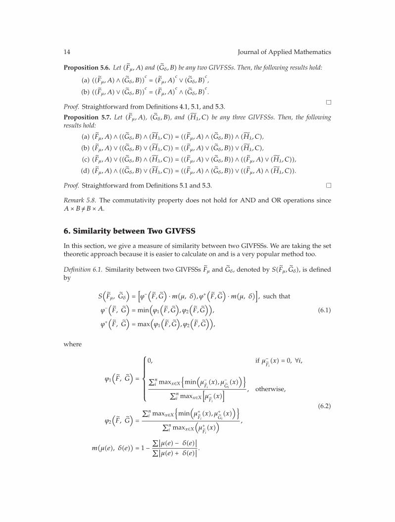
14 Journal of Applied Mathematics
Proposition 5.6. Let ( ˜Fμ,A) and ( ˜Gδ, B) be any two GIVFSSs. Then, the following results hold:
(a) (( ˜Fμ,A) ∧ ( ˜Gδ, B))c= ( ˜Fμ,A)
c ∨ ( ˜Gδ, B)c,
(b) (( ˜Fμ,A) ∨ ( ˜Gδ, B))c= ( ˜Fμ,A)
c ∧ ( ˜Gδ, B)c.
Proof. Straightforward from Definitions 4.1, 5.1, and 5.3.
Proposition 5.7. Let ( ˜Fμ,A), ( ˜Gδ, B), and (˜Hλ,C) be any three GIVFSSs. Then, the followingresults hold:
(a) ( ˜Fμ,A) ∧ (( ˜Gδ, B) ∧ (˜Hλ,C)) = (( ˜Fμ,A) ∧ ( ˜Gδ, B)) ∧ (˜Hλ,C),
(b) ( ˜Fμ,A) ∨ (( ˜Gδ, B) ∨ (˜Hλ,C)) = (( ˜Fμ,A) ∨ ( ˜Gδ, B)) ∨ (˜Hλ,C),
(c) ( ˜Fμ,A) ∨ (( ˜Gδ, B) ∧ (˜Hλ,C)) = (( ˜Fμ,A) ∨ ( ˜Gδ, B)) ∧ (( ˜Fμ,A) ∨ (˜Hλ,C)),
(d) ( ˜Fμ,A) ∧ (( ˜Gδ, B) ∨ (˜Hλ,C)) = (( ˜Fμ,A) ∧ ( ˜Gδ, B)) ∨ (( ˜Fμ,A) ∧ (˜Hλ,C)).
Proof. Straightforward from Definitions 5.1 and 5.3.
Remark 5.8. The commutativity property does not hold for AND and OR operations sinceA × B /=B ×A.
6. Similarity between Two GIVFSS
In this section, we give a measure of similarity between two GIVFSSs. We are taking the settheoretic approach because it is easier to calculate on and is a very popular method too.
Definition 6.1. Similarity between two GIVFSSs ˜Fμ and ˜Gδ, denoted by S( ˜Fμ, ˜Gδ), is definedby
S(
˜Fμ, ˜Gδ
)
=[
ϕ−(
˜F, ˜G)
·m(μ, δ), ϕ+(
˜F, ˜G)
·m(μ, δ)]
, such that
ϕ−(
˜F, ˜G)
= min(
ϕ1
(
˜F, ˜G)
, ϕ2
(
˜F, ˜G))
,
ϕ+(
˜F, ˜G)
= max(
ϕ1
(
˜F, ˜G)
, ϕ2
(
˜F, ˜G))
,
(6.1)
where
ϕ1
(
˜F, ˜G)
=
⎧
⎪
⎪
⎪
⎪
⎪
⎪
⎨
⎪
⎪
⎪
⎪
⎪
⎪
⎩
0, if μ−˜Fi(x) = 0, ∀i,
∑ni maxx∈X
{
min(
μ−˜Fi(x), μ−
˜Gi(x)
)}
∑ni maxx∈X
[
μ−˜Fi(x)
] , otherwise,
ϕ2
(
˜F, ˜G)
=
∑ni maxx∈X
{
min(
μ+˜Fi(x), μ+
˜Gi(x)
)}
∑ni maxx∈X
(
μ+˜Fi(x)
) ,
m(
μ(e), δ(e))
= 1 −∑∣
∣μ(e) − δ(e)∣
∣
∑∣
∣μ(e) + δ(e)∣
∣
.
(6.2)

Journal of Applied Mathematics 15
Definition 6.2. Let ˜Fμ and ˜Gδ be two GIVFSSs over the same universe (U,E). We say that twoGIVFSS are significantly similar if ϕ−( ˜F, ˜G) ·m(μ, δ) � 1/2.
Theorem 6.3. Let ˜Fμ, ˜Gδ, and ˜Hλ be any three GIVFSSs over (U,E). Then, the following hold:
(a) in general S( ˜Fμ, ˜Gδ)/=S( ˜Gδ, ˜Fμ),
(b) ϕ−( ˜F, ˜G) ≥ 0 and ϕ+( ˜F, ˜G) ≤ 1,
(c) ˜Fμ = ˜Gδ ⇒ S( ˜Fμ, ˜Gδ) = 1,
(d) ˜Fμ ⊆ ˜Gδ ⊆ ˜Hλ ⇒ S( ˜Fμ,˜Hλ) � S( ˜Gδ,˜Hλ),
(e) ˜Fμ˜∩ ˜Gδ = ∅ ⇔ S( ˜Fμ, ˜Gδ) = 0.
Proof. (a) The proof is straightforward and follows from Definition 6.1.(b) From Definition 6.1, we have
ϕ1
(
˜F, ˜G)
=
⎧
⎪
⎪
⎪
⎪
⎪
⎨
⎪
⎪
⎪
⎪
⎪
⎩
0, if μ−˜Fi(x) = 0, ∀i,
∑ni maxx∈X
{
min(
μ−˜Fi(x), μ−
˜Gi(x)
)}
∑ni maxx∈X
(
μ−˜Fi(x)
) , otherwise.(6.3)
If μ−˜Fi(x) = 0, for all i, then ϕ−( ˜F, ˜G) = 0, and, if μ−
˜Fi(x)/= 0, for some i, then it is clear
that ϕ−( ˜F, ˜G) ≥ 0.Also since ϕ+( ˜F, ˜G) = max(ϕ1( ˜F, ˜G), ϕ2( ˜F, ˜G)), suppose that ϕ1( ˜F, ˜G) = 1 and
ϕ2( ˜F, ˜G) = 1, then ϕ+( ˜F, ˜G) = 1, that means, if ϕ1( ˜F, ˜G) < 1 and ϕ2( ˜F, ˜G) < 1, thenϕ+( ˜F, ˜G) ≤ 1.
(c) The proof is straightforward and follows from Definition 6.1.(d) The proof is straightforward and follows from Definition 6.1.(e) The proof is straightforward and follows from Definition 6.1.
Example 6.4. Let ˜Fμ be GIVFSS over (U,E) defined as follows:
˜Fμ(e1) =({
x1
[0.3, 0.7],
x2
[0.4, 0.8],
x3
[0.1, 0.3]
}
, 0.4)
,
˜Fμ(e2) =({
x1
[0.5, 0.6],
x2
[0.1, 0.3],
x3
[0, 0.4]
}
, 0.6)
,
˜Fμ(e3) =({
x1
[0.7, 0.9],
x2
[0.1, 0.5],
x3
[0.8, 1]
}
, 0.8)
.
(6.4)

16 Journal of Applied Mathematics
Let ˜Gδ be another GIVFSS over (U,E) defined as follows:
˜Gδ(e1) =({
x1
[0.1, 0.4],
x2
[0.5, 0.7],
x3
[0.2, 0.3]
}
, 0.3)
,
˜Gδ(e2) =({
x1
[0.6, 0.8],
x2
[0.5, 0.6],
x3
[0.4, 0.8]
}
, 0.7)
,
˜Gδ(e3) =({
x1
[0.4, 0.7],
x2
[0.3, 0.5],
x3
[0.5, 0.7]
}
, 0.6)
.
(6.5)
Here,
m(
μ(e), δ(e))
= 1 −∑∣
∣μ(e) − δ(e)∣
∣
∑∣
∣μ(e) + δ(e)∣
∣
= 1 − |(0.4 − 0.3)| + |(0.6 − 0.7)| + |(0.8 − 0.6)||(0.4 + 0.3)| + |(0.6 + 0.7)| + |(0.80 + 0.6)|
∼= 0.8824,
ϕ1
(
˜F, ˜G)
=(max{min(0.3, 0.1),min(0.4, 0.5),min(0.1, 0.2)}
max(0.3, 0.4, 0.1) +max(0.5, 0.1, 0) +max(0.7, 0.1, 0.8)
+max{min(0.5, 0.6),min(0.1, 0.5),min(0, 0.4)}
max(0.3, 0.4, 0.1) +max(0.5, 0.1, 0) +max(0.7, 0.1, 0.8)
+max{min(0.7, 0.4),min(0.1, 0.3),min(0.8, 0.5)})
max(0.3, 0.4, 0.1) +max(0.5, 0.1, 0) +max(0.7, 0.1, 0.8)
=max{0.1, 0.4, 0.1} +max{0.5, 0.1, 0} +max{0.4, 0.1, 0.5}max(0.3, 0.4, 0.1) +max(0.5, 0.1, 0) +max(0.7, 0.1, 0.8)
=0.4 + 0.5 + 0.50.4 + 0.5 + 0.8
= 0.824,
ϕ2
(
˜F, ˜G)
=(max{min(0.7, 0.4),min(0.8, 0.7),min(0.3, 0.3)}
max(0.7, 0.8, 0.3) +max(0.6, 0.3, 0.4) +max(0.9, 0.5, 1)
+max{min(0.6, 0.8),min(0.3, 0.6),min(0.4, 0.8)}
max(0.7, 0.8, 0.3) +max(0.6, 0.3, 0.4) +max(0.9, 0.5, 1)
+max{min(0.9, 0.7),min(0.5, 0.5),min(1, 0.7)})
max(0.7, 0.8, 0.3) +max(0.6, 0.3, 0.4) +max(0.9, 0.5, 1)
=max{0.4, 0.7, 0.3} +max{0.6, 0.3, 0.4} +max{0.7, 0.5, 0.7}max(0.7, 0.8, 0.3) +max(0.6, 0.3, 0.4) +max(0.9, 0.5, 1)
=0.7 + 0.6 + 0.70.8 + 0.6 + 1
= 0.833.
(6.6)

Journal of Applied Mathematics 17
Then,
ϕ−(
˜F, ˜G)
= min(
ϕ1
(
˜F, ˜G)
, ϕ2
(
˜F, ˜G))
= min(0.824, 0.833) = 0.824,
ϕ+(
˜F, ˜G)
= max(
ϕ1
(
˜F, ˜G)
, ϕ2
(
˜F, ˜G))
= max(0.824, 0.833) = 0.833.(6.7)
Hence, the similarity between the two GIVFSSs ˜Fμ and ˜Gδ will be
S(
˜Fμ, ˜Gδ
)
=[
ϕ−(
˜F, ˜G)
·m(μ, δ), ϕ+(
˜F, ˜G)
·m(μ, δ)]
= [(0.824) · (0.8824), (0.833) · (0.8824)]
= [0.727, 0.735].
(6.8)
Therefore, ˜Fμ and ˜Gδ are significantly similar.
7. Application of Similarity Measure in Medical Diagnosis
In this section, we will try to estimate the possibility that a sick person having certain visiblesymptoms is suffering from dengue fever. For this, we first construct a GIVFSS model fordengue fever and the GIVFSS of symptoms for the sick person. Next, we find the similaritymeasure of these two sets. If they are significantly similar, then we conclude that the personis possibly suffering from dengue fever. Let our universal set contain only two elements“yes” and “no,” that is, U = {y, n}. Here, the set of parameters E is the set of certainvisible symptoms. Let E = {e1, e2, e3, e4, e5, e6, e7}, where e1 = body temperature, e2 = coughwith chest congestion, e3 = loose motion, e4 = chills, e5 = headache, e6 = low heart rate(bradycardia), and e7 = pain upon moving the eyes. Our model GIVFSS for dengue feverMμ is given in Table 4, and this can be prepared with the help of a physician.
Now, after talking to the sick person, we can construct his GIVFSS Gδ as in Table 5.Now, we find the similarity measure of these two sets by using the same method as
in Example 6.4, where, after the calculation, we get ϕ−(˜M, ˜G)m(μ, δ) ∼= 0.22 < 1/2. Hencethe two GIVFSSs are not significantly similar. Therefore, we conclude that the person is notsuffering from dengue fever.
8. Conclusion
In this paper, we have introduced the concept of generalised interval-valued fuzzy soft setand studied some of its properties. The complement, union, intersection, “AND,” and “OR”operations have been defined on the interval-valued fuzzy soft sets. An application of thistheory is given in solving a decision making problem. Similarity measure of two generalisedinterval-valued fuzzy soft sets is discussed, and its application to medical diagnosis has beenshown.
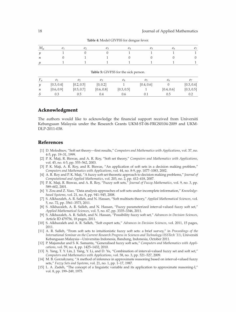
18 Journal of Applied Mathematics
Table 4: Model GIVFSS for dengue fever.
Mμ e1 e2 e3 e4 e5 e6 e7
y 1 0 0 1 1 1 1n 0 1 1 0 0 0 0μ 1 1 1 1 1 1 1
Table 5: GIVFSS for the sick person.
Fα e1 e2 e3 e4 e5 e6 e7
y [0.3, 0.4] [0.2, 0.5] [0, 0.2] 1 [0.4, 0.6] 0 [0.3, 0.4]n [0.6, 0.9] [0.5, 0.7] [0.6, 0.8] [0.3, 0.5] 1 [0.4, 0.6] [0.3, 0.5]δ 0.3 0.5 0.4 0.6 0.1 0.5 0.2
Acknowledgment
The authors would like to acknowledge the financial support received from UniversitiKebangsaan Malaysia under the Research Grants UKM-ST-06-FRGS0104-2009 and UKM-DLP-2011-038.
References
[1] D. Molodtsov, “Soft set theory—first results,” Computers and Mathematics with Applications, vol. 37, no.4-5, pp. 19–31, 1999.
[2] P. K. Maji, R. Biswas, and A. R. Roy, “Soft set theory,” Computers and Mathematics with Applications,vol. 45, no. 4-5, pp. 555–562, 2003.
[3] P. K. Maji, A. R. Roy, and R. Biswas, “An application of soft sets in a decision making problem,”Computers and Mathematics with Applications, vol. 44, no. 8-9, pp. 1077–1083, 2002.
[4] A. R. Roy and P. K. Maji, “A fuzzy soft set theoretic approach to decision making problems,” Journal ofComputational and Applied Mathematics, vol. 203, no. 2, pp. 412–418, 2007.
[5] P. K. Maji, R. Biswas, and A. R. Roy, “Fuzzy soft sets,” Journal of Fuzzy Mathematics, vol. 9, no. 3, pp.589–602, 2001.
[6] Y. Zou and Z. Xiao, “Data analysis approaches of soft sets under incomplete information,” Knowledge-based Systems, vol. 21, no. 8, pp. 941–945, 2008.
[7] S. Alkhazaleh, A. R. Salleh, and N. Hassan, “Soft multisets theory,” Applied Mathematical Sciences, vol.5, no. 72, pp. 3561–3573, 2011.
[8] S. Alkhazaleh, A. R. Salleh, and N. Hassan, “Fuzzy parameterized interval-valued fuzzy soft set,”Applied Mathematical Sciences, vol. 5, no. 67, pp. 3335–3346, 2011.
[9] S. Alkhazaleh, A. R. Salleh, and N. Hassan, “Possibility fuzzy soft set,” Advances in Decision Sciences,Article ID 479756, 18 pages, 2011.
[10] S. Alkhazaleh and A. R. Salleh, “Soft expert sets,” Advances in Decision Sciences, vol. 2011, 15 pages,2011.
[11] A. R. Salleh, “From soft sets to intuitionistic fuzzy soft sets: a brief survey,” in Proceedings of theInternational Seminar on the Current Research Progress in Sciences and Technology (ISSTech ’11), UniversitiKebangsaan Malaysia—Universitas Indonesia, Bandung, Indonesia, October 2011.
[12] P. Majumdar and S. K. Samanta, “Generalised fuzzy soft sets,” Computers and Mathematics with Appli-cations, vol. 59, no. 4, pp. 1425–1432, 2010.
[13] X. Yang, T. Y. Lin, J. Yang, Y. Li, and D. Yu, “Combination of interval-valued fuzzy set and soft set,”Computers and Mathematics with Applications, vol. 58, no. 3, pp. 521–527, 2009.
[14] M. B. Gorzałczany, “A method of inference in approximate reasoning based on interval-valued fuzzysets,” Fuzzy Sets and Systems, vol. 21, no. 1, pp. 1–17, 1987.
[15] L. A. Zadeh, “The concept of a linguistic variable and its application to approximate reasoning-I,”vol. 8, pp. 199–249, 1975.

Submit your manuscripts athttp://www.hindawi.com
Hindawi Publishing Corporationhttp://www.hindawi.com Volume 2014
MathematicsJournal of
Hindawi Publishing Corporationhttp://www.hindawi.com Volume 2014
Mathematical Problems in Engineering
Hindawi Publishing Corporationhttp://www.hindawi.com
Differential EquationsInternational Journal of
Volume 2014
Applied MathematicsJournal of
Hindawi Publishing Corporationhttp://www.hindawi.com Volume 2014
Probability and StatisticsHindawi Publishing Corporationhttp://www.hindawi.com Volume 2014
Journal of
Hindawi Publishing Corporationhttp://www.hindawi.com Volume 2014
Mathematical PhysicsAdvances in
Complex AnalysisJournal of
Hindawi Publishing Corporationhttp://www.hindawi.com Volume 2014
OptimizationJournal of
Hindawi Publishing Corporationhttp://www.hindawi.com Volume 2014
CombinatoricsHindawi Publishing Corporationhttp://www.hindawi.com Volume 2014
International Journal of
Hindawi Publishing Corporationhttp://www.hindawi.com Volume 2014
Operations ResearchAdvances in
Journal of
Hindawi Publishing Corporationhttp://www.hindawi.com Volume 2014
Function Spaces
Abstract and Applied AnalysisHindawi Publishing Corporationhttp://www.hindawi.com Volume 2014
International Journal of Mathematics and Mathematical Sciences
Hindawi Publishing Corporationhttp://www.hindawi.com Volume 2014
The Scientific World JournalHindawi Publishing Corporation http://www.hindawi.com Volume 2014
Hindawi Publishing Corporationhttp://www.hindawi.com Volume 2014
Algebra
Discrete Dynamics in Nature and Society
Hindawi Publishing Corporationhttp://www.hindawi.com Volume 2014
Hindawi Publishing Corporationhttp://www.hindawi.com Volume 2014
Decision SciencesAdvances in
Discrete MathematicsJournal of
Hindawi Publishing Corporationhttp://www.hindawi.com
Volume 2014 Hindawi Publishing Corporationhttp://www.hindawi.com Volume 2014
Stochastic AnalysisInternational Journal of