Thermal Decomposition in 1D Shear Flow of Generalised ...

Thermal Decomposition in 1D Shear Flow of Generalised Newtonian

Fluids

Adeleke Olusegun Bankole ([email protected])African Institute for Mathematical Sciences (AIMS)

Supervised by: Doctor Tirivanhu Chinyoka

University of Cape Town, South Africa.

22 May 2009

Submitted in partial fulfillment of a postgraduate diploma at AIMS

Abstract

The effect of variable viscosity in a thermally decomposable generalised Newtonian fluids (GNF) sub-jected to unsteady 1D shear flow is investigated by direct numerical simulations. A numerical algorithmbased on the semi-implicit finite-difference scheme is implemented in time and space using the temper-ature corrected Carreau model equation as the model for variable viscosity. The chemical kinetics isassumed to follow the Arrhenius rate equation; this reaction is assumed to be exothermic. Approximate(Numerical) and graphical results are presented for some parameters in the problem, thermal criticalityconditions are also discussed. It is observed that increasing the non-Newtonian nature of the fluid helpsto delay the onset of thermal runaway when compared to Newtonian nature of the fluid.

Keywords: Thermally decomposable; Unsteady flow; Variable viscosity; Arrhenius chemical kinetics;Semi-implicit finite-difference scheme; Direct numerical simulations; Carreau model; Thermal runaway;Generalised Newtonian fluids(GNF)

Declaration

I, the undersigned, hereby declare that the work contained in this essay is my original work, and thatany work done by others or by myself previously has been acknowledged and referenced accordingly.

Adeleke Olusegun Bankole, 22 May 2009

i

Contents

Abstract i

1 Introduction 1

1.1 Motivation for Study . . . . . . . . . . . . . . . . . . . . . . . . . . . . . . . . . . . . 1

1.2 Newtonian Fluids . . . . . . . . . . . . . . . . . . . . . . . . . . . . . . . . . . . . . . 2

1.3 Generalised Newtonian Fluids . . . . . . . . . . . . . . . . . . . . . . . . . . . . . . . . 3

1.3.1 Shear Thinning and Shear Thickening . . . . . . . . . . . . . . . . . . . . . . . 3

2 Governing Equations 5

2.1 Continuity Equation . . . . . . . . . . . . . . . . . . . . . . . . . . . . . . . . . . . . . 5

2.2 Momentum Equation . . . . . . . . . . . . . . . . . . . . . . . . . . . . . . . . . . . . 6

2.3 Energy Equation . . . . . . . . . . . . . . . . . . . . . . . . . . . . . . . . . . . . . . . 7

2.4 Dimensionless Equations . . . . . . . . . . . . . . . . . . . . . . . . . . . . . . . . . . 7

3 Numerical Solution and Discussion 10

3.1 Finite-Difference Scheme . . . . . . . . . . . . . . . . . . . . . . . . . . . . . . . . . . 10

3.2 Finite-Difference Approximation to Derivatives . . . . . . . . . . . . . . . . . . . . . . . 11

3.2.1 Difference Formulas . . . . . . . . . . . . . . . . . . . . . . . . . . . . . . . . . 11

3.3 Power Law . . . . . . . . . . . . . . . . . . . . . . . . . . . . . . . . . . . . . . . . . . 14

3.4 Carreau Model . . . . . . . . . . . . . . . . . . . . . . . . . . . . . . . . . . . . . . . . 15

3.5 Code Validation . . . . . . . . . . . . . . . . . . . . . . . . . . . . . . . . . . . . . . . 15

3.6 Sensitivity in Parameters . . . . . . . . . . . . . . . . . . . . . . . . . . . . . . . . . . 17

3.6.1 Effects of Reynolds Number in Convergence . . . . . . . . . . . . . . . . . . . . 17

3.6.2 Effects of Peclet Number in Convergence . . . . . . . . . . . . . . . . . . . . . 17

3.6.3 Effects of Brinkman Number in Convergence . . . . . . . . . . . . . . . . . . . 17

3.6.4 Reaction Parameter . . . . . . . . . . . . . . . . . . . . . . . . . . . . . . . . . 19

3.6.5 Variation in Time Constant . . . . . . . . . . . . . . . . . . . . . . . . . . . . . 20

3.6.6 Effects of Behaviour Index . . . . . . . . . . . . . . . . . . . . . . . . . . . . . 20

3.6.7 Blow up of Solutions/Thermal Runaway . . . . . . . . . . . . . . . . . . . . . . 22

4 Conclusion 25

ii

A Numerical Codes Written in PYTHON 26

A.1 Code for Power Law Plot . . . . . . . . . . . . . . . . . . . . . . . . . . . . . . . . . . 26

A.2 Code for Carreau Plot . . . . . . . . . . . . . . . . . . . . . . . . . . . . . . . . . . . . 26

A.3 Code for Constant and Variable Viscosity . . . . . . . . . . . . . . . . . . . . . . . . . . 27

A.4 Code for Variation of Parameters . . . . . . . . . . . . . . . . . . . . . . . . . . . . . . 29

A.5 Code for Thermal Runaway . . . . . . . . . . . . . . . . . . . . . . . . . . . . . . . . . 32

References 37

iii

1. Introduction

1.1 Motivation for Study

The study of thermal decomposition of a viscous reactive fluid through parallel media is paramount inunderstanding the hydrodynamics of engineering processes [11]. Most generalised Newtonian fluids usedin engineering and industrial processes become reactive during flow (i.e. when fluid is subjected to shearsome of the work done is dissipated as heat) this makes them thermally decomposable e.g hydrocarbonsand esters. Heat is generated internally within the fluid causing an increase in temperature within thefluid, the chemical reactions within the fluid follows mainly from the Arrhenius kinetics. Fluid propertiessuch as viscosity is dependent on the temperature variation from time to time. Fluids in which theviscosity additionally depends on applied shear rates are called generalised Newtonian fluids . In thisproject we model this physical phenomena through a plane Couette flow, that is, flow between twoparallel plates with the upper plate moving and the lower plate kept stationary. The fluid flow in thechannel is thus driven only by the motion of the upper plate. A constant pressure is maintained withinthe channel. A lot of work has been done in the study of steady state flows problems e.g. [11, 12],where by steady flow we mean a fully developed flow in which the velocity, temperature etc. no longerdepend on time. Currently, due mainly to well developed computational solution methods, attentionhas largely shifted to the study of unsteady flow problems.

Unsteady flows are gradually becoming the main focus of attention in computational rheology studies.The fast development of polymeric materials and associated polymer processing operations in the pastdecades has evoked significant research endeavors on the study of non-Newtonian fluid mechanics [10,13]. The flow and motion of viscous reactive fluid between two plates occurs mostly in engineeringand science applications. This process occurs practically in diverse areas e.g. in thermal applications— heat exchangers, cooling and drying technology, heating and air-conditioning techniques, in medicalapplications — subdomains of biomedicine and medical engineering, in chemical reactions — polymermelts, polmerisation reactor, catalyzers and in geological applications — extraction of oil and gas ingeological fields [3].

The objectives of this project are to:

• Document the effects of variable viscosity in the thermal decomposition of relevant liquids sub-jected to unsteady one-dimensional shear flow and chemical reactions.

• Determine whether the particular constitutive modelling of viscosity (e.g via the Power Law,Carreau Model) play any significant role in such thermal decomposition.

The appropriate governing equations for the fluid flow will be solved via semi-implicit finite-differenceschemes. A similar investigation was recently carried out on constant viscosity elastic fluids, see Chinyoka[2] it was demonstrated that fluid elasticity progressively delayed the onset of thermal decomposition.Possible future work thus arises via the extension to variable viscosity elastic liquids. We start off witha brief discussion of the characterisation of fluids as either Newtonian or non-Newtonian.

1

Section 1.2. Newtonian Fluids Page 2

1.2 Newtonian Fluids

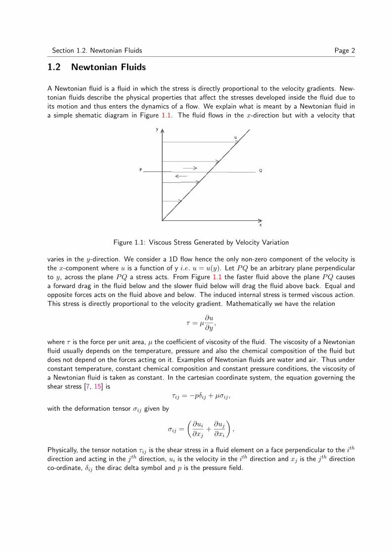
A Newtonian fluid is a fluid in which the stress is directly proportional to the velocity gradients. New-tonian fluids describe the physical properties that affect the stresses developed inside the fluid due toits motion and thus enters the dynamics of a flow. We explain what is meant by a Newtonian fluid ina simple shematic diagram in Figure 1.1. The fluid flows in the x-direction but with a velocity that

Figure 1.1: Viscous Stress Generated by Velocity Variation

varies in the y-direction. We consider a 1D flow hence the only non-zero component of the velocity isthe x-component where u is a function of y i.e. u = u(y). Let PQ be an arbitrary plane perpendicularto y, across the plane PQ a stress acts. From Figure 1.1 the faster fluid above the plane PQ causesa forward drag in the fluid below and the slower fluid below will drag the fluid above back. Equal andopposite forces acts on the fluid above and below. The induced internal stress is termed viscous action.This stress is directly proportional to the velocity gradient. Mathematically we have the relation

τ = µ∂u

∂y,

where τ is the force per unit area, µ the coefficient of viscosity of the fluid. The viscosity of a Newtonianfluid usually depends on the temperature, pressure and also the chemical composition of the fluid butdoes not depend on the forces acting on it. Examples of Newtonian fluids are water and air. Thus underconstant temperature, constant chemical composition and constant pressure conditions, the viscosity ofa Newtonian fluid is taken as constant. In the cartesian coordinate system, the equation governing theshear stress [7, 15] is

τij = −pδij + µσij ,

with the deformation tensor σij given by

σij =(∂ui∂xj

+∂uj∂xi

),

Physically, the tensor notation τij is the shear stress in a fluid element on a face perpendicular to the ith

direction and acting in the jth direction, ui is the velocity in the ith direction and xj is the jth directionco-ordinate, δij the dirac delta symbol and p is the pressure field.

Section 1.3. Generalised Newtonian Fluids Page 3

1.3 Generalised Newtonian Fluids

Any fluid that deviates from the above description is called a non-Newtonian fluid. These fluids havestructural features which are influenced by the flow; this behaviour can arise in liquids with long molecules(polymers) and in liquids where the molecules tends to gather in more organised structures than usual. Adistinguishing characteristic of various non-Newtonian fluid is the dependence of the apparent viscosityon the rate of strain. The dependence of the apparent viscosity on the rate of strain is a major concern inmany applications and it can be modelled using fairly a straightforward modifications of the constitutiveequation for a Newtonian fluid, the resulting equations describe the generalized Newtonian fluids. Ageneralized Newtonian fluid differs from a Newtonian fluid only in that the viscosity exhibits shear ratedependence while in Newtonian fluids viscosity is constant. We should however remark that the viscosityof any fluid additionally depends on the temperature, pressure and chemical composition.

1.3.1 Shear Thinning and Shear Thickening

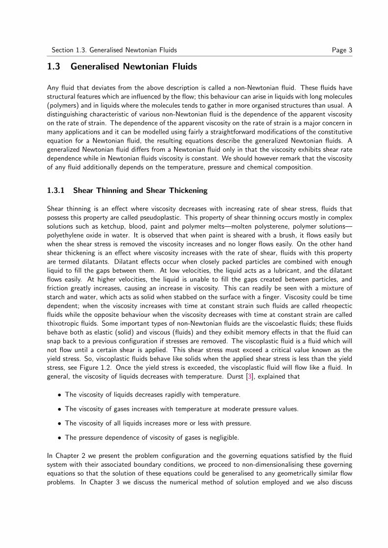
Shear thinning is an effect where viscosity decreases with increasing rate of shear stress, fluids thatpossess this property are called pseudoplastic. This property of shear thinning occurs mostly in complexsolutions such as ketchup, blood, paint and polymer melts—molten polysterene, polymer solutions—polyethylene oxide in water. It is observed that when paint is sheared with a brush, it flows easily butwhen the shear stress is removed the viscosity increases and no longer flows easily. On the other handshear thickening is an effect where viscosity increases with the rate of shear, fluids with this propertyare termed dilatants. Dilatant effects occur when closely packed particles are combined with enoughliquid to fill the gaps between them. At low velocities, the liquid acts as a lubricant, and the dilatantflows easily. At higher velocities, the liquid is unable to fill the gaps created between particles, andfriction greatly increases, causing an increase in viscosity. This can readily be seen with a mixture ofstarch and water, which acts as solid when stabbed on the surface with a finger. Viscosity could be timedependent; when the viscosity increases with time at constant strain such fluids are called rheopecticfluids while the opposite behaviour when the viscosity decreases with time at constant strain are calledthixotropic fluids. Some important types of non-Newtonian fluids are the viscoelastic fluids; these fluidsbehave both as elastic (solid) and viscous (fluids) and they exhibit memory effects in that the fluid cansnap back to a previous configuration if stresses are removed. The viscoplastic fluid is a fluid which willnot flow until a certain shear is applied. This shear stress must exceed a critical value known as theyield stress. So, viscoplastic fluids behave like solids when the applied shear stress is less than the yieldstress, see Figure 1.2. Once the yield stress is exceeded, the viscoplastic fluid will flow like a fluid. Ingeneral, the viscosity of liquids decreases with temperature. Durst [3], explained that

• The viscosity of liquids decreases rapidly with temperature.

• The viscosity of gases increases with temperature at moderate pressure values.

• The viscosity of all liquids increases more or less with pressure.

• The pressure dependence of viscosity of gases is negligible.

In Chapter 2 we present the problem configuration and the governing equations satisfied by the fluidsystem with their associated boundary conditions, we proceed to non-dimensionalising these governingequations so that the solution of these equations could be generalised to any geometrically similar flowproblems. In Chapter 3 we discuss the numerical method of solution employed and we also discuss

Section 1.3. Generalised Newtonian Fluids Page 4

Figure 1.2: Properties of Newtonian and non-Newtonian Fluids [3].

the non-Newtonian models (Power Law and the Carreau model). We present and summarise the mainresults in Chapter 4.

2. Governing Equations

In this chapter we discuss the problem configuration, the governing equations together with the associ-ated boundary conditions. We then proceed to non-dimensionalise the equations.

We consider the plane Couette flow in Figure 2.1 below

Figure 2.1: Problem Configuration

The geometry of the problem is such that the fluid is confined between two plates. The upper platemoves with velocity u = U and the lower plate is stationary, u = 0. The boundary conditions arethus that the walls at y = 0, y = L move with velocities 0 and U respectively and are maintained atthe same temperature T0. A viscous reactive fluid is enclosed between the plates and the velocity ofthe fluid is driven by the motion of the upper plate “a condition known as the no-slip boundary”, theresulting velocity profile in a plane Couette flow, which predicts a linear velocity profile. As this fluidis sheared some of the workdone is dissipated as heat hence causing an increase in temperature withinthe fluid so we therefore assume that the heat is purely an internally generated heat, there exist noexternal heat through the plates (i.e. no suction or injection). We model this flow as 1D with velocitycomponent (u(t, y), 0, 0). In this model the ratio of the channel width to the channel length is 1giving a small aspect ratio that is ε = L/L0 1 (see Figure 2.1) where L0 is the typical length scaleof the channel and L is the typical width scale. The thermal conductivity, specific heat capacity anddensity of the liquid is represented by k, cp and ρ respectively but will be treated as constant whilethe viscosity µ(T, γ) of the fluid is temperature and shear rate dependent. Table 2 shows some usefultypical parameter notation [5].

2.1 Continuity Equation

The equation describing the conservation of scalar quantities such as mass M is obtained from theconcept of a control volume. A control volume is any closed region in space. It is a region in whichthe rate of accumulation of mass is equal to the net rate at which the mass enters it by crossingthe boundaries. The size and shape of a control volume may vary with time, and the control volumeboundaries need not correspond to physical interfaces. Consider a fluid of density ρ, velocity u in anarbitrary control volume Ω, conservation of mass requires that∫

Ω

(∂

∂tρ+∇·uρ

)dV. = 0

5

Section 2.2. Momentum Equation Page 6

Table 2.1: Typical Parameter and Notations

Symbol Name Unit

ρ Fluid density kgm−3

µ0 Typical dynamic viscosity kgm−1s−1

µ Dynamic viscosity kgm−1s−1

ε Aspect ratio of the flow DimensionlessU Velocity scale ms−1

T Temperature K∆T Temperature drop Kt Time sL Channel height mL0 Channel length mk Thermal conductivity Wm−1K−1

cp Heat capacity Jkg−1K−1

Re = ρUL/µ Reynolds number DimensionlessPe = ρcpLU/k Peclet number DimensionlessPr = µcp/k Prandtl number DimensionlessBr = µU2/k∆T Brinkman number Dimensionless

This holds for any arbitrary control volume Ω, Hence,

∂

∂tρ+∇· ρu = 0.

For incompressible fluid ρ = constant and continuity equation reduces to

∇·u = 0. (2.1)

2.2 Momentum Equation

The momentum equations are obtained from Newtons second law relating the total forces acting on afluid element to the mass and acceleration of the fluid element. Neglecting body forces, the generalisedmomentum equations in cartesian coordinates are given by x, y and z momentum components [3].

x-momentum component is

ρDu

Dt= −∂P

∂x+

∂

∂x

2µ∂u

∂x− 2

3µ(∇·u)

+

∂

∂y

µ

(∂u

∂y+∂v

∂x

)+

∂

∂z

µ

(∂w

∂x+∂u

∂z

),

y-momentum component is

ρDv

Dt= −∂P

∂y+

∂

∂y

2µ∂v

∂y− 2

3µ(∇·u)

+

∂

∂z

µ

(∂v

∂z+∂w

∂y

)+

∂

∂x

µ

(∂u

∂y+∂v

∂x

),

z-momentum component is

ρDw

Dt= −∂P

∂z+

∂

∂z

2µ∂w

∂z− 2

3µ(∇·u)

+

∂

∂x

µ

(∂w

∂x+∂u

∂z

)+

∂

∂y

µ

(∂v

∂z+∂w

∂y

),

Section 2.3. Energy Equation Page 7

where µ is the coefficient of viscosity and P the pressure. In our case, flow is 1D that is u = (u(t, y), 0, 0),and P is constant. The x-momentum equation reduces to

ρDu

Dt=

∂

∂y

(µ(T, γ)

∂u

∂y

),

whereD

Dt=

∂

∂t+u· ∇ is the material derivative however u· ∇ vanishes. Hence the momentum equation

reduces to

ρ∂u

∂t=

∂

∂y

(µ(T, γ)

∂u

∂y

). (2.2)

with the corresponding boundary conditions u(0) = 0, u(L) = U .

2.3 Energy Equation

In the energy equation we include source terms based on the Arrhenius kinetics

ρCpDT

Dt= k

∂2T

∂y2+QC0Ae

− ERT + µ(T, γ)

(∂u

∂y

)2

,

Making use of the definition of material derivative, we obtain the energy equation

ρCp∂T

∂t= k

∂2T

∂y2+QC0Ae

− ERT + µ(T, γ)

(∂u

∂y

)2

, (2.3)

with the boundary conditions T (0) = T0 and T (L) = T0.

where R the gas constant known as Boltzman gas constant, T the temperature in degree Kelvin, Athe Arrhenius constant described as the pre-exponential factor (total number of collision leading toa reaction per second), E the activation energy which the colliding molecules must attain before achemical reaction must take place, Cp is the heat capacity, k is the thermal conductivity, Q is the Heatflux and C0 is the residual concentration of reactants. This reaction within the fluid is exothermic.

2.4 Dimensionless Equations

Equations (2.1), (2.2) and (2.3) are dimensional equations of motion governing the incompressiblefluid in the narrow channel. They form a set of coupled, nonlinear, partial differential equations. Theformidable problems encountered in solving this full set of non-linear equations is not made any easierby the number of parameters included in the problem. The number of parameters can be reduced byintroducing dimensionless groups. We introduce the following dimensionless variables into equations(2.1), (2.2) and (2.3) to get the non-dimensional equations of motion [11]

x′ =x

L, y′ =

y

L, u′ =

u

U, t′ =

tU

L, µ(Θ)′ =

µ(Θ)µ0

The superscript ′ represents dimensionless quantities.

Θ′ =E(T − T0)

RT 20

, λ =QEAL2C0e

− ERT0

RT 20 k

, β =µ0U

2eERT0

QAL2C0, ε =

RT0

E

Section 2.4. Dimensionless Equations Page 8

where λ, β, ε represent the Frank-Kamenetskii parameter, viscous heating parameter and the activationenergy parameter respectively. The Frank-Kamenetskii parameter measures how reactive reactants are.The non-dimensional equations are obtained as follows:

• Continuity equation

∂u′

∂x′= 0

• Momentun equation

Uρ∂(u′U)∂(t′L)

=∂

∂(y′L)

(µ(Θ, γ)

∂(u′U)∂(y′L)

)∂u′

∂t′=

µ0

ρUL

∂

∂y′

(µ(Θ, γ)′

∂u′

∂y′

)Hence the dimensionless equation for momentum is given as

∂u′

∂t′=

1Re

∂

∂y′

(µ(Θ, γ)′

∂u′

∂y′

)(2.4)

• Energy Equation

Non-dimensionalising the LHS in equation (2.3) we obtain

∂T

∂t=RT 2

0U

EL

∂Θ′

∂t′

Non-dimensionalising the first term of RHS in equation (2.3) we obtain

∂T 2

∂y2=RT 2

0U

EL2

∂2Θ′

∂y′2

For the coupled velocity term in equation (2.3) we obtain(∂u

∂y

)2

=U2

L2

(∂u′

∂y′

)2

.

For the reaction term in (2.3) we obtain

QC0Ae− ERT =

λεT0k

L2e

Θ′1+εΘ′ .

Substituting into the energy equation (2.3) we have

ρCpU∂Θ′

∂t′=k

L

∂2Θ′

∂y′2+λk

Le

Θ′1+εΘ′ + µ(Θ, γ)

λβk

L

(∂u′

∂y′

)2

.

Isolating∂Θ′

∂t′we obtain

∂Θ′

∂t′=

k

ρCpUL

∂2Θ′

∂y′2+

λk

ρCpULe

Θ′1+εΘ′ + µ(Θ, γ)

λβk

ρCpUL

(∂u′

∂y′

)2

,

Section 2.4. Dimensionless Equations Page 9

Pe∂Θ′

∂t′=∂2Θ′

∂y′2+ λe

Θ′1+εΘ′ + µ(Θ, γ)Br

(∂u′

∂y′

)2

, (2.5)

where Pe = RePr = (ρUL/µ) (Cpµ/k) = ρCpUL/k is the Peclet number, Re is the Reynoldsnumber, Pr is the Prandtl number and Br is the Brinkman number

For convenience, we drop the ′ superscript notation in (2.4) and (2.5).

∂u

∂x= 0, (2.6)

Re∂u

∂t=

∂

∂y

(µ(Θ, γ)

∂u

∂y

), (2.7)

Pe∂Θ∂t

=∂2Θ∂y2

+ λeΘ

1+εΘ + µ(Θ, γ)Br(∂u

∂y

)2

, (2.8)

µ(Θ, γ) is the dimensionless temperature and shear rate dependent viscosity.

Therefore equations (2.6), (2.7) and (2.8) corresponds to the dimensionless governing equations for thevelocity u and temperature T with boundary conditions.

u(0) = 0, u(1) = 1, (2.9)

Θ(0) = Θ(1) = 0. (2.10)

The following chapter introduces the numerical method of solution used in solving these coupled dimen-sionless equations, (2.6− 2.8) subject to boundary conditions (2.9− 2.10) and discusses the sensitivityof some parameters in the solution.

3. Numerical Solution and Discussion

In this chapter we discuss the finite-difference scheme used for the numerical integration of the coupleddifferential equations. We proceed to treat the the non-Newtonian models; the Power Law and theCarreau Model of viscosity and we explain the results obtained.

3.1 Finite-Difference Scheme

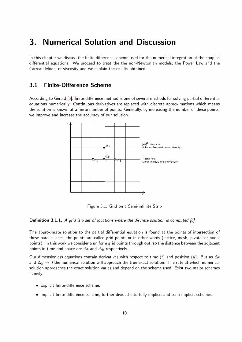
According to Gerald [6], finite-difference method is one of several methods for solving partial differentialequations numerically. Continuous derivatives are replaced with discrete approximations which meansthe solution is known at a finite number of points. Generally, by increasing the number of these points,we improve and increase the accuracy of our solution.

Figure 3.1: Grid on a Semi-infinite Strip

Definition 3.1.1. A grid is a set of locations where the discrete solution is computed [6]

The approximate solution to the partial differential equation is found at the points of intersection ofthese parallel lines, the points are called grid points or in other words (lattice, mesh, pivotal or nodalpoints). In this work we consider a uniform grid points through out, so the distance between the adjacentpoints in time and space are ∆t and ∆y respectively.

Our dimensionless equations contain derivatives with respect to time (t) and position (y). But as ∆tand ∆y → 0 the numerical solution will approach the true exact solution. The rate at which numericalsolution approaches the exact solution varies and depend on the scheme used. Exist two major schemesnamely:

• Explicit finite-difference scheme;

• Implicit finite-difference scheme, further divided into fully implicit and semi-implicit schemes.

10

Section 3.2. Finite-Difference Approximation to Derivatives Page 11

In this work we consider the semi-implicit scheme because it allows flexibility in values for r = ∆t/(∆y)2

(called the Courant number) and improves numerical stability.

3.2 Finite-Difference Approximation to Derivatives

We will consider the forward in time—center in space (FTCS) approximation to our derivatives.

3.2.1 Difference Formulas

First Order Forward Difference

By Taylor series expansion of u(y) about the point yi

u(yi + δy) = u(yi) + δy∂u

∂y

∣∣∣∣yi

+δy2

2!∂2u

∂y2

∣∣∣∣yi

+δy3

3!∂3u

∂y3

∣∣∣∣yi

+ . . .

u(yi − δy) = u(yi)− δy∂u

∂y

∣∣∣∣yi

+δy2

2!∂2u

∂y2

∣∣∣∣yi

− δy3

3!∂3u

∂y3

∣∣∣∣yi

+ . . .

where δy = ∆y, we obtain

u(yi + ∆y) = u(yi) + ∆y∂u

∂y

∣∣∣∣yi

+∆y2

2!∂2u

∂y2

∣∣∣∣yi

+∆y3

3!∂3u

∂y3

∣∣∣∣yi

+ . . .

u(yi + ∆y) = u(yi)−∆y∂u

∂y

∣∣∣∣yi

+∆y2

2!∂2u

∂y2

∣∣∣∣yi

− ∆y3

3!∂3u

∂y3

∣∣∣∣yi

+ . . .

Solving for∂u

∂y

∣∣∣∣yi

we obtain

∂u

∂y

∣∣∣∣yi

=u(yi + ∆y)− u(yi)

∆y− ∆y2

2!∂2u

∂y2

∣∣∣∣yi

− ∆y3

3!∂3u

∂y3

∣∣∣∣yi

+ . . .

If we substitute the approximate solution, that is ui ≈ u(yi) and ui+1 ≈ u(yi+1) we obtain

∂u

∂y

∣∣∣∣yi

≈ ui+1 − ui∆y

− ∆y2

2!∂2u

∂y2

∣∣∣∣yi

− ∆y3

3!∂3u

∂y3

∣∣∣∣yi

+ . . .

So we have,

∂u

∂y

∣∣∣∣yi

=ui+1 − ui

∆y+O(y) (3.1)

Equation (3.1) is the forward difference formula for (∂u/∂y)yi because it involves nodes yi and yi+1


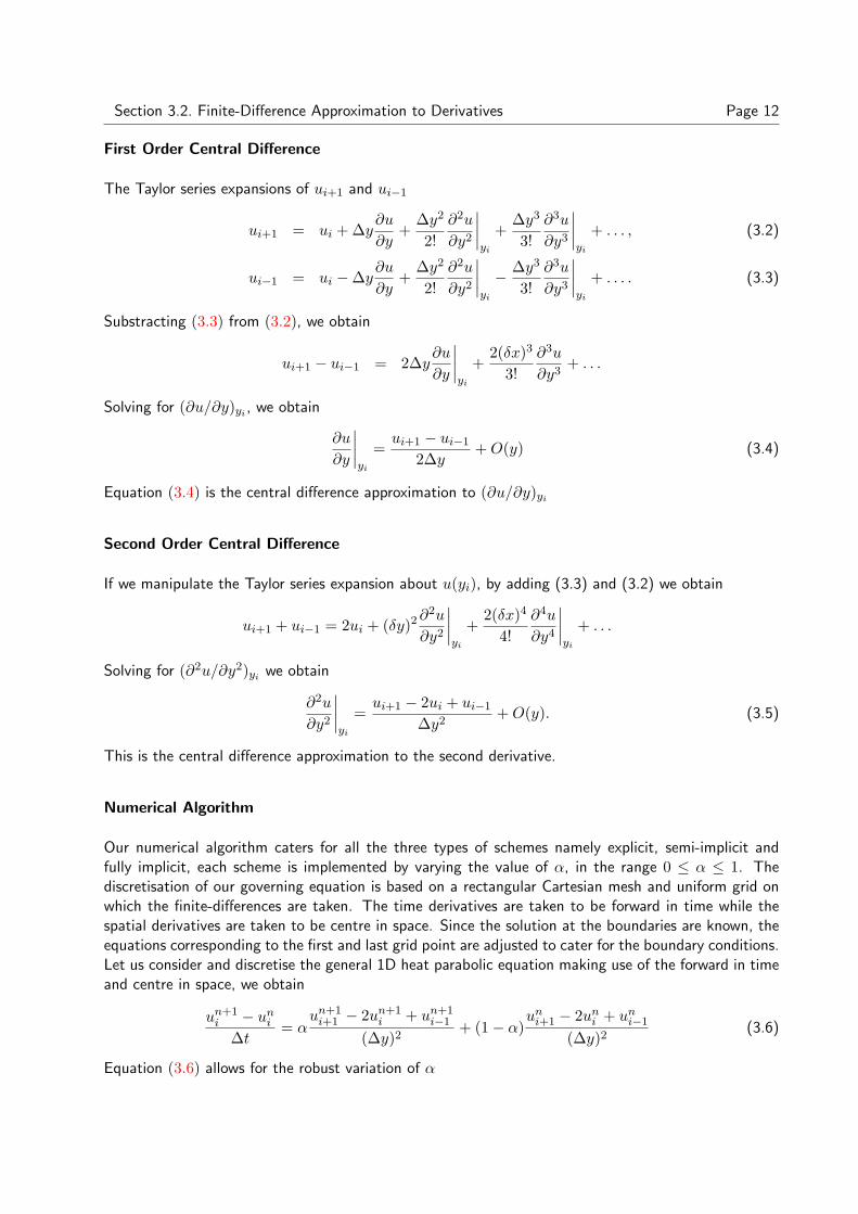
First Order Central Difference

The Taylor series expansions of ui+1 and ui−1

ui+1 = ui + ∆y∂u

∂y+

∆y2

2!∂2u

∂y2

∣∣∣∣yi

+∆y3

3!∂3u

∂y3

∣∣∣∣yi

+ . . . , (3.2)

ui−1 = ui −∆y∂u

∂y+

∆y2

2!∂2u

∂y2

∣∣∣∣yi

− ∆y3

3!∂3u

∂y3

∣∣∣∣yi

+ . . . . (3.3)

Substracting (3.3) from (3.2), we obtain

ui+1 − ui−1 = 2∆y∂u

∂y

∣∣∣∣yi

+2(δx)3

3!∂3u

∂y3+ . . .

Solving for (∂u/∂y)yi , we obtain

∂u

∂y

∣∣∣∣yi

=ui+1 − ui−1

2∆y+O(y) (3.4)

Equation (3.4) is the central difference approximation to (∂u/∂y)yi

Second Order Central Difference

If we manipulate the Taylor series expansion about u(yi), by adding (3.3) and (3.2) we obtain

ui+1 + ui−1 = 2ui + (δy)2∂2u

∂y2

∣∣∣∣yi

+2(δx)4

4!∂4u

∂y4

∣∣∣∣yi

+ . . .

Solving for (∂2u/∂y2)yi we obtain

∂2u

∂y2

∣∣∣∣yi

=ui+1 − 2ui + ui−1

∆y2+O(y). (3.5)

This is the central difference approximation to the second derivative.

Numerical Algorithm

Our numerical algorithm caters for all the three types of schemes namely explicit, semi-implicit andfully implicit, each scheme is implemented by varying the value of α, in the range 0 ≤ α ≤ 1. Thediscretisation of our governing equation is based on a rectangular Cartesian mesh and uniform grid onwhich the finite-differences are taken. The time derivatives are taken to be forward in time while thespatial derivatives are taken to be centre in space. Since the solution at the boundaries are known, theequations corresponding to the first and last grid point are adjusted to cater for the boundary conditions.Let us consider and discretise the general 1D heat parabolic equation making use of the forward in timeand centre in space, we obtain

un+1i − uni

∆t= α

un+1i+1 − 2un+1

i + un+1i−1

(∆y)2+ (1− α)

uni+1 − 2uni + uni−1

(∆y)2(3.6)

Equation (3.6) allows for the robust variation of α


• When α = 0 the scheme reduces to the fully explicit scheme

• When α =12

the scheme reduces to the Crank Nicolson scheme

• When α = 1 the scheme reduces to the fully-implicit scheme

Where (n+12

) is obtained by taking the average of (n+ 1) and (n)

Rearranging (3.6) and collecting the explicit terms to the right hand side to obtain the unknown termswe have

− αrun+1i+1 + (1 + 2αr)un+1

i − αrun+1i−1 = (1− α)runi+1 + (1− 2(1− α)r)uni + (1− α)runi−1 (3.7)

where r = ∆t/(∆y)2. If we apply this scheme to (2.7) and (2.8) for both velocity and energy (temper-ature) equation we obtain

−αrµ(n)un+1i+1 + (Re+ 2αrµ(n))un+1

i − αrµ(n)un+1i−1 = (1− α)rµ(n)uni+1+

(Re− 2(1− α)rµ(n))uni + (1− α)rµ(n)uni−1+r

4(uni+1 − uni−1

) (µ

(n)i+1 − µ

(n)i−1

) (3.8)

−αrΘn+1i+1 + (Pe+ 2αr)Θn+1

i − αrΘn+1i−1 = (1− α)rΘn

i+1+

(Pe− 2(1− α)r)Θni + (1− α)rΘn

i−1 + ∆tλ exp(

Θni

1 + εΘni

)+ ∆tµ(n)Br

(uni+1 − uni−1

2∆y

)2 (3.9)

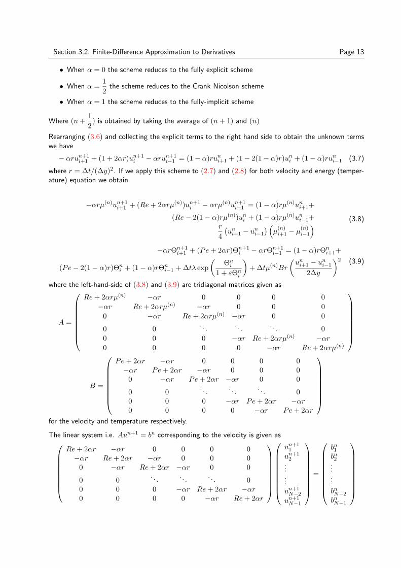
where the left-hand-side of (3.8) and (3.9) are tridiagonal matrices given as

A =

Re+ 2αrµ(n) −αr 0 0 0 0−αr Re+ 2αrµ(n) −αr 0 0 0

0 −αr Re+ 2αrµ(n) −αr 0 0

0 0. . .

. . .. . . 0

0 0 0 −αr Re+ 2αrµ(n) −αr0 0 0 0 −αr Re+ 2αrµ(n)

B =

Pe+ 2αr −αr 0 0 0 0−αr Pe+ 2αr −αr 0 0 0

0 −αr Pe+ 2αr −αr 0 0

0 0. . .

. . .. . . 0

0 0 0 −αr Pe+ 2αr −αr0 0 0 0 −αr Pe+ 2αr

for the velocity and temperature respectively.

The linear system i.e. Aun+1 = bn corresponding to the velocity is given as

Re+ 2αr −αr 0 0 0 0−αr Re+ 2αr −αr 0 0 0

0 −αr Re+ 2αr −αr 0 0

0 0. . .

. . .. . . 0

0 0 0 −αr Re+ 2αr −αr0 0 0 0 −αr Re+ 2αr

un+11

un+12

...

...

un+1N−2

un+1N−1

=

bn1bn2......bnN−2

bnN−1

Section 3.3. Power Law Page 14

The linear system BΘn+1 = gn corresponding to the temperature is given as

Pe+ 2αr −αr 0 0 0 0−αr Pe+ 2αr −αr 0 0 0

0 −αr Pe+ 2αr −αr 0 0

0 0. . .

. . .. . . 0

0 0 0 −αr Pe+ 2αr −αr0 0 0 0 −αr Pe+ 2αr

Θn+11

Θn+12

...

...

Θn+1N−2

Θn+1N−1

=

gn1gn2......gnN−2

gnN−1

where bn and gn are the explicit terms of the velocity and temperature respectively. Equations (3.8)and (3.9) are solved by inversion of the tridiagonal matrices to obtain the solutions un+1 and Θn+1.

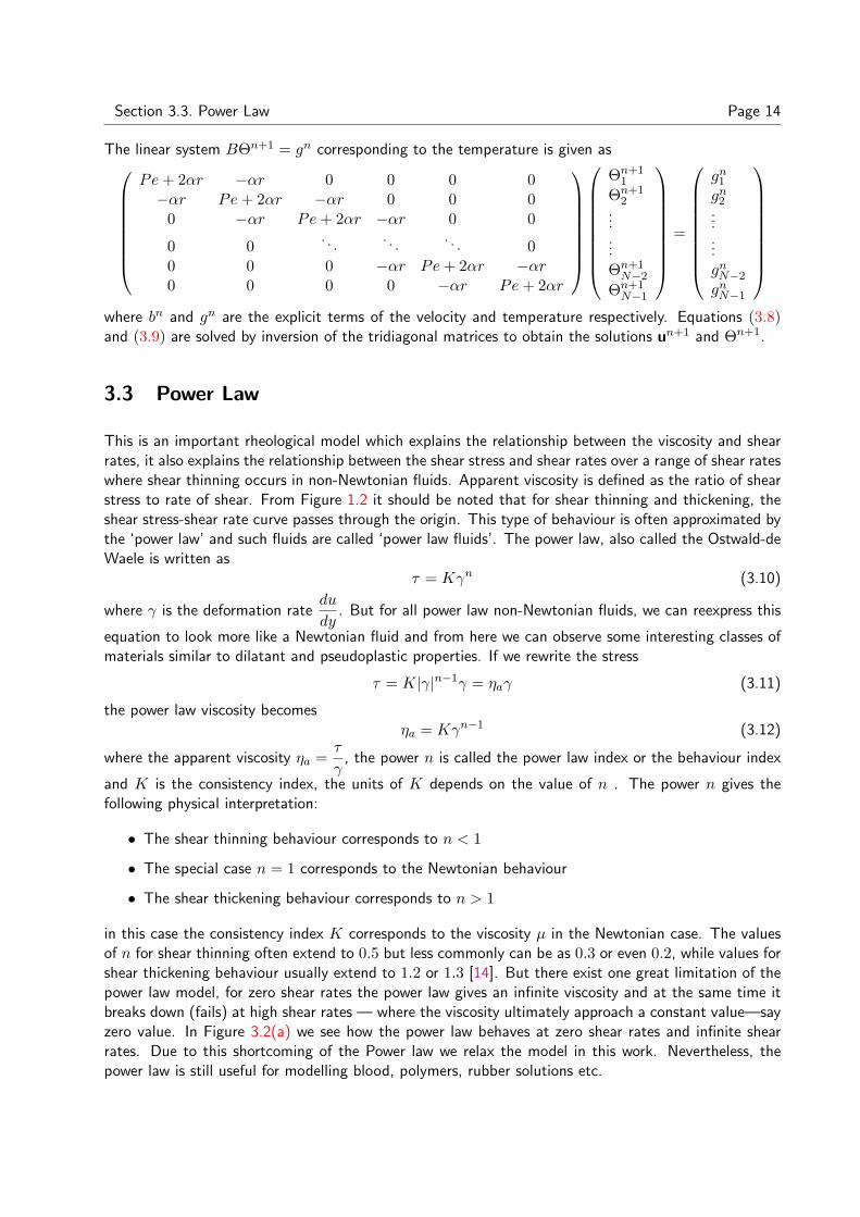
3.3 Power Law

This is an important rheological model which explains the relationship between the viscosity and shearrates, it also explains the relationship between the shear stress and shear rates over a range of shear rateswhere shear thinning occurs in non-Newtonian fluids. Apparent viscosity is defined as the ratio of shearstress to rate of shear. From Figure 1.2 it should be noted that for shear thinning and thickening, theshear stress-shear rate curve passes through the origin. This type of behaviour is often approximated bythe ‘power law’ and such fluids are called ‘power law fluids’. The power law, also called the Ostwald-deWaele is written as

τ = Kγn (3.10)

where γ is the deformation ratedu

dy. But for all power law non-Newtonian fluids, we can reexpress this

equation to look more like a Newtonian fluid and from here we can observe some interesting classes ofmaterials similar to dilatant and pseudoplastic properties. If we rewrite the stress

τ = K|γ|n−1γ = ηaγ (3.11)

the power law viscosity becomesηa = Kγn−1 (3.12)

where the apparent viscosity ηa =τ

γ, the power n is called the power law index or the behaviour index

and K is the consistency index, the units of K depends on the value of n . The power n gives thefollowing physical interpretation:

• The shear thinning behaviour corresponds to n < 1

• The special case n = 1 corresponds to the Newtonian behaviour

• The shear thickening behaviour corresponds to n > 1

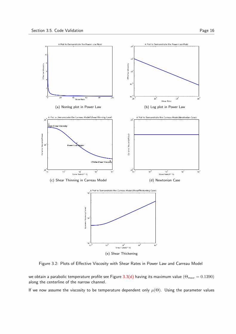
in this case the consistency index K corresponds to the viscosity µ in the Newtonian case. The valuesof n for shear thinning often extend to 0.5 but less commonly can be as 0.3 or even 0.2, while values forshear thickening behaviour usually extend to 1.2 or 1.3 [14]. But there exist one great limitation of thepower law model, for zero shear rates the power law gives an infinite viscosity and at the same time itbreaks down (fails) at high shear rates — where the viscosity ultimately approach a constant value—sayzero value. In Figure 3.2(a) we see how the power law behaves at zero shear rates and infinite shearrates. Due to this shortcoming of the Power law we relax the model in this work. Nevertheless, thepower law is still useful for modelling blood, polymers, rubber solutions etc.

Section 3.4. Carreau Model Page 15

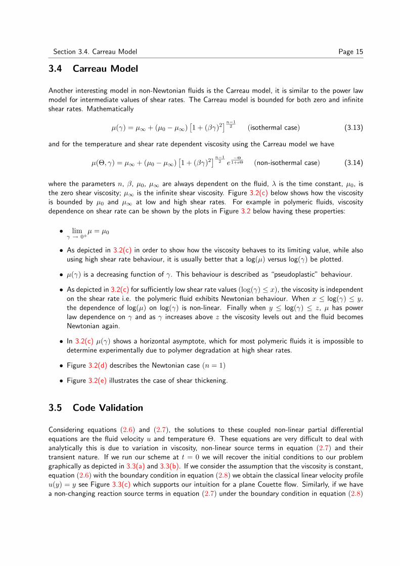
3.4 Carreau Model

Another interesting model in non-Newtonian fluids is the Carreau model, it is similar to the power lawmodel for intermediate values of shear rates. The Carreau model is bounded for both zero and infiniteshear rates. Mathematically

µ(γ) = µ∞ + (µ0 − µ∞)[1 + (βγ)2

]n−12 (isothermal case) (3.13)

and for the temperature and shear rate dependent viscosity using the Carreau model we have

µ(Θ, γ) = µ∞ + (µ0 − µ∞)[1 + (βγ)2

]n−12 e

−Θ1+εΘ (non-isothermal case) (3.14)

where the parameters n, β, µ0, µ∞ are always dependent on the fluid, λ is the time constant, µ0, isthe zero shear viscosity; µ∞ is the infinite shear viscosity. Figure 3.2(c) below shows how the viscosityis bounded by µ0 and µ∞ at low and high shear rates. For example in polymeric fluids, viscositydependence on shear rate can be shown by the plots in Figure 3.2 below having these properties:

• limγ → 0+

µ = µ0

• As depicted in 3.2(c) in order to show how the viscosity behaves to its limiting value, while alsousing high shear rate behaviour, it is usually better that a log(µ) versus log(γ) be plotted.

• µ(γ) is a decreasing function of γ. This behaviour is described as “pseudoplastic” behaviour.

• As depicted in 3.2(c) for sufficiently low shear rate values (log(γ) ≤ x), the viscosity is independenton the shear rate i.e. the polymeric fluid exhibits Newtonian behaviour. When x ≤ log(γ) ≤ y,the dependence of log(µ) on log(γ) is non-linear. Finally when y ≤ log(γ) ≤ z, µ has powerlaw dependence on γ and as γ increases above z the viscosity levels out and the fluid becomesNewtonian again.

• In 3.2(c) µ(γ) shows a horizontal asymptote, which for most polymeric fluids it is impossible todetermine experimentally due to polymer degradation at high shear rates.

• Figure 3.2(d) describes the Newtonian case (n = 1)

• Figure 3.2(e) illustrates the case of shear thickening.

3.5 Code Validation

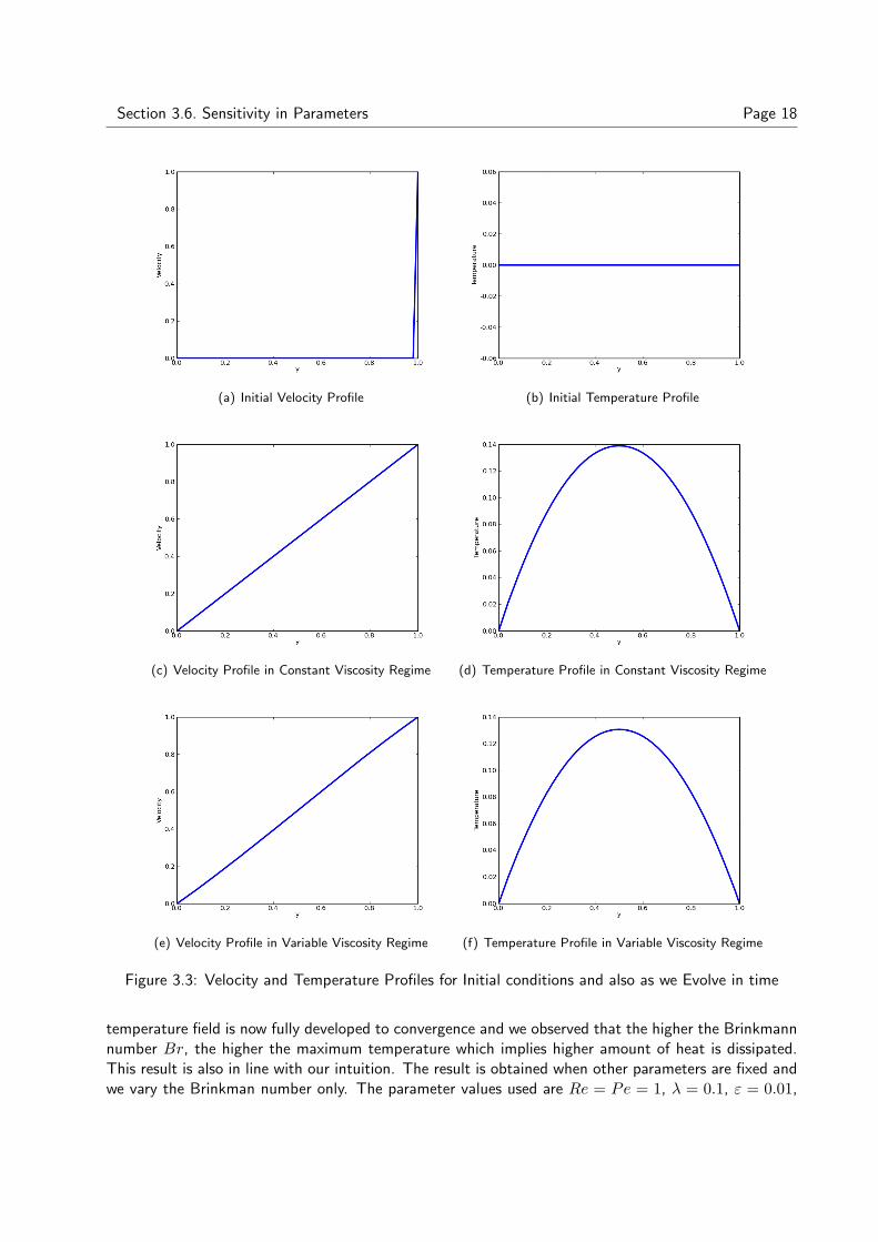
Considering equations (2.6) and (2.7), the solutions to these coupled non-linear partial differentialequations are the fluid velocity u and temperature Θ. These equations are very difficult to deal withanalytically this is due to variation in viscosity, non-linear source terms in equation (2.7) and theirtransient nature. If we run our scheme at t = 0 we will recover the initial conditions to our problemgraphically as depicted in 3.3(a) and 3.3(b). If we consider the assumption that the viscosity is constant,equation (2.6) with the boundary condition in equation (2.8) we obtain the classical linear velocity profileu(y) = y see Figure 3.3(c) which supports our intuition for a plane Couette flow. Similarly, if we havea non-changing reaction source terms in equation (2.7) under the boundary condition in equation (2.8)

Section 3.5. Code Validation Page 16

(a) Nonlog plot in Power Law (b) Log plot in Power Law

(c) Shear Thinning in Carreau Model (d) Newtonian Case

(e) Shear Thickening

Figure 3.2: Plots of Effective Viscosity with Shear Rates in Power Law and Carreau Model

we obtain a parabolic temperature profile see Figure 3.3(d) having its maximum value (Θmax = 0.1390)along the centerline of the narrow channel.

If we now assume the viscosity to be temperature dependent only µ(Θ). Using the parameter values

Section 3.6. Sensitivity in Parameters Page 17

Re = Pe = Br = 1, λ = 0.1, ε = 0.01, ∆y = 0.02 and ∆t = 0.001 we still obtain the linear velocityprofile and the parabolic temperature profile. We observe that at these parameter values the constantviscosity gave the maximum temperature Θmax = 0.1390 and for the variable viscosity we observe thatthe maximum temperature decreases slightly to Θmax = 0.1308. Infact, the maximum temperature,Θmax converges to 0.1308 for any value of t ≥ 0.6 for the variable viscosity (temperature only). Thecomputational speed is of order of few seconds as we refine the meshes on a standard computer.

3.6 Sensitivity in Parameters

3.6.1 Effects of Reynolds Number in Convergence

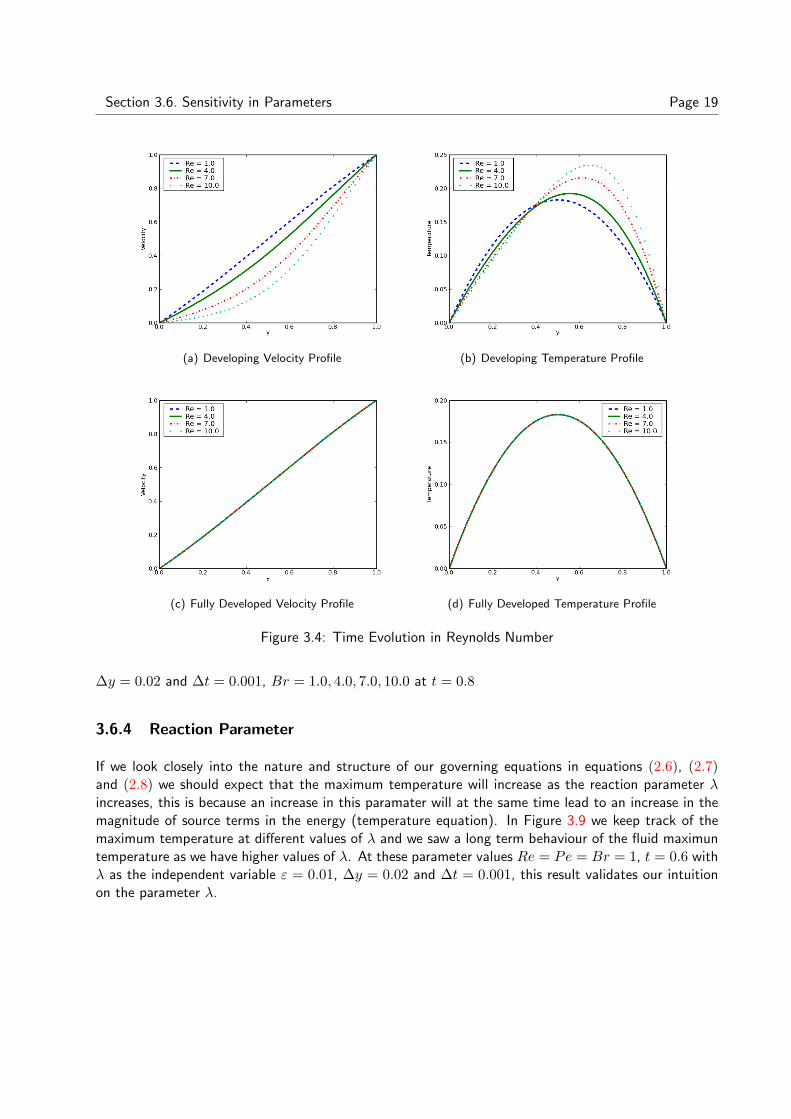
Reynolds number is a measure of of the relative importance of inertial and viscous effects in steadyflows. Alternatively, it is a measure of the relative importance of the convective and diffusive transportof momentum [8]. Inertial (or convective) effects tends to be prominent when Re 1 and nearlyabsent when Re 1. In Figures 3.4(a) and 3.4(b) we obtain the developing velocity and temperatureprofiles at t = 0.8, but as we evolve in time all the profiles at different typical Reynolds numberRe = 1.0, 4.0, 7.0, 10.0 converges to the same maximum teperature at t = 20 in Figures 3.4(c) and3.4(d). The parameter values for these profiles are Pe = Br = 1, λ = 0.1, ε = 0.01, ∆y = 0.02and ∆t = 0.001. Hence we say, the Reynolds number does not play a significant role in the thermaldecomposition in our problem configuration and this is true if we consider the governing equations inthe velocity equation (2.7), the Reynolds number is only a scalar multiplication of the time dependentvelocity scale.

3.6.2 Effects of Peclet Number in Convergence

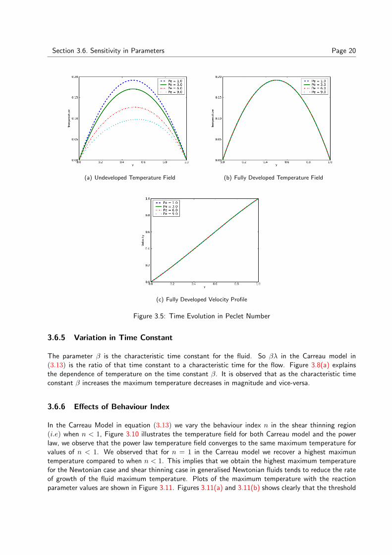
The Peclet number indicates the importance of convection relative to conduction or diffussion [8].Alternatively, because Peclet number is the coefficient of the convective terms, it evidently shows theimportance of convection relative to the molecular transport processes. If the Peclet number Pe is > 1this implies the convective term is dominant and vice-versa. In Figure 3.5 we observed that the higherthe Peclet number Pe the lesser the maximum temperature attained but we also observed that as weevolve in time to convergence the conduction terms balances the convective terms and the temperaturefield converges for all values of Pe to the same maximum temperature. The parameter values used areRe = Br = 1, λ = 0.1, ε = 0.01, ∆y = 0.02 and ∆t = 0.001 at t = 0.8 for the developing profile,we run it to convergence (steady state solution) at t = 20 for Pe = 1.0, 3.0, 6.0, 9.0. Similarly as theReynolds number, in this range of values, the parameter does not play a significant role in the thermaldecomposition.

3.6.3 Effects of Brinkman Number in Convergence

The Brinkman number Br expressses the relative importance of viscous dissipation and heat conduction.This occurs only in the energy equation, so higher values of the Brinkman parameter are expected tolead to an increase in the amount of heat generated within the fluid. Since this effect is caused byviscous dissipation (internal friction) the heat generated will be in form of mechanical heat as the fluidis sheared. This is shown in Figure 3.6. Figure 3.6(a) shows when the flow is not fully developed, we sawsome variations in the velocity profile and the temperature field and Figure 3.6(b) shows when the fluid


(a) Initial Velocity Profile (b) Initial Temperature Profile

(c) Velocity Profile in Constant Viscosity Regime (d) Temperature Profile in Constant Viscosity Regime

(e) Velocity Profile in Variable Viscosity Regime (f) Temperature Profile in Variable Viscosity Regime

Figure 3.3: Velocity and Temperature Profiles for Initial conditions and also as we Evolve in time

temperature field is now fully developed to convergence and we observed that the higher the Brinkmannnumber Br, the higher the maximum temperature which implies higher amount of heat is dissipated.This result is also in line with our intuition. The result is obtained when other parameters are fixed andwe vary the Brinkman number only. The parameter values used are Re = Pe = 1, λ = 0.1, ε = 0.01,


(a) Developing Velocity Profile (b) Developing Temperature Profile

(c) Fully Developed Velocity Profile (d) Fully Developed Temperature Profile

Figure 3.4: Time Evolution in Reynolds Number

∆y = 0.02 and ∆t = 0.001, Br = 1.0, 4.0, 7.0, 10.0 at t = 0.8

3.6.4 Reaction Parameter

If we look closely into the nature and structure of our governing equations in equations (2.6), (2.7)and (2.8) we should expect that the maximum temperature will increase as the reaction parameter λincreases, this is because an increase in this paramater will at the same time lead to an increase in themagnitude of source terms in the energy (temperature equation). In Figure 3.9 we keep track of themaximum temperature at different values of λ and we saw a long term behaviour of the fluid maximuntemperature as we have higher values of λ. At these parameter values Re = Pe = Br = 1, t = 0.6 withλ as the independent variable ε = 0.01, ∆y = 0.02 and ∆t = 0.001, this result validates our intuitionon the parameter λ.


(a) Undeveloped Temperature Field (b) Fully Developed Temperature Field

(c) Fully Developed Velocity Profile

Figure 3.5: Time Evolution in Peclet Number

3.6.5 Variation in Time Constant

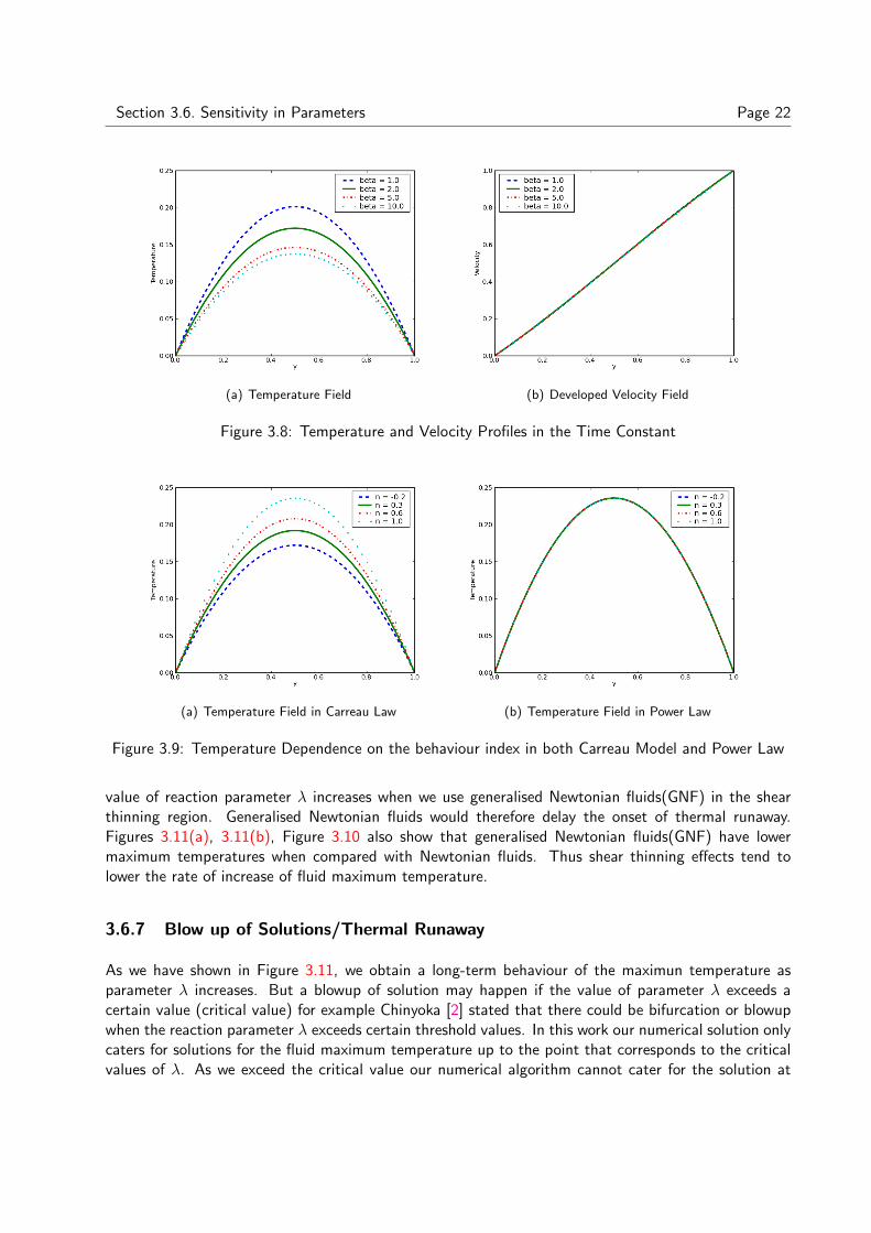
The parameter β is the characteristic time constant for the fluid. So βλ in the Carreau model in(3.13) is the ratio of that time constant to a characteristic time for the flow. Figure 3.8(a) explainsthe dependence of temperature on the time constant β. It is observed that as the characteristic timeconstant β increases the maximum temperature decreases in magnitude and vice-versa.

3.6.6 Effects of Behaviour Index

In the Carreau Model in equation (3.13) we vary the behaviour index n in the shear thinning region(i.e) when n < 1, Figure 3.10 illustrates the temperature field for both Carreau model and the powerlaw, we observe that the power law temperature field converges to the same maximum temperature forvalues of n < 1. We observed that for n = 1 in the Carreau model we recover a highest maximuntemperature compared to when n < 1. This implies that we obtain the highest maximum temperaturefor the Newtonian case and shear thinning case in generalised Newtonian fluids tends to reduce the rateof growth of the fluid maximum temperature. Plots of the maximum temperature with the reactionparameter values are shown in Figure 3.11. Figures 3.11(a) and 3.11(b) shows clearly that the threshold


(a) Developing Velocity Profile (b) Developing Temperature Profile

(c) Fully Developed Velocity Profile (d) Fully Developed Temperature Profile

Figure 3.6: Time Evolution in Brinkman Number

(a) (b)

Figure 3.7: (a) Velocity Profile in Reaction Parameter Variation, (b) Temperature Profile in ReactionParameter Variation


(a) Temperature Field (b) Developed Velocity Field

Figure 3.8: Temperature and Velocity Profiles in the Time Constant

(a) Temperature Field in Carreau Law (b) Temperature Field in Power Law

Figure 3.9: Temperature Dependence on the behaviour index in both Carreau Model and Power Law

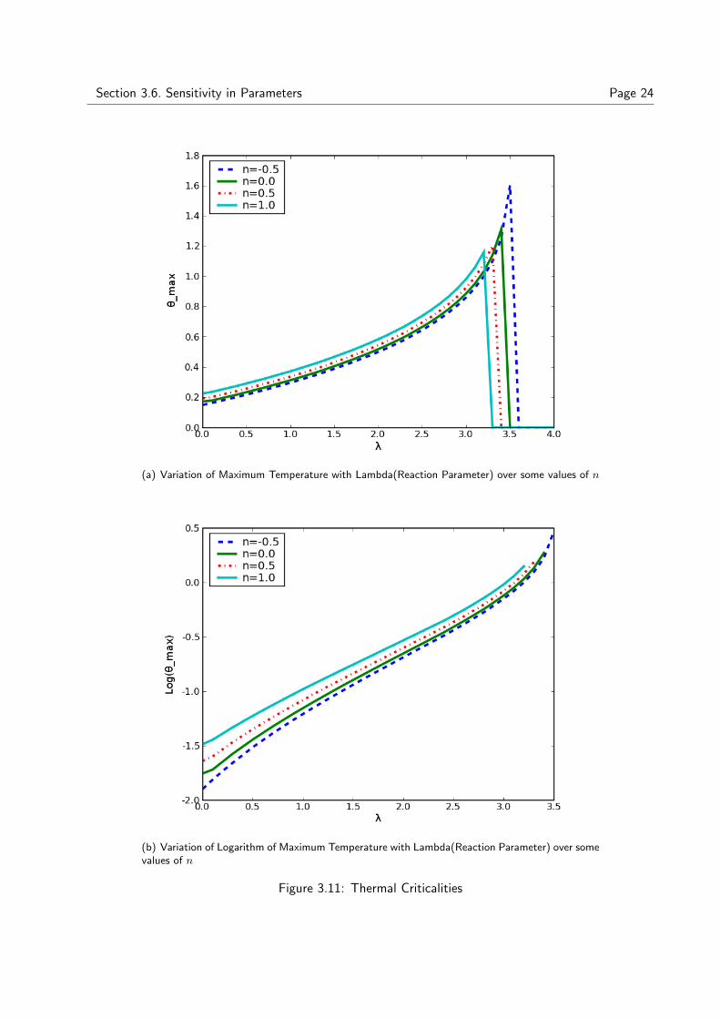
value of reaction parameter λ increases when we use generalised Newtonian fluids(GNF) in the shearthinning region. Generalised Newtonian fluids would therefore delay the onset of thermal runaway.Figures 3.11(a), 3.11(b), Figure 3.10 also show that generalised Newtonian fluids(GNF) have lowermaximum temperatures when compared with Newtonian fluids. Thus shear thinning effects tend tolower the rate of increase of fluid maximum temperature.

3.6.7 Blow up of Solutions/Thermal Runaway

As we have shown in Figure 3.11, we obtain a long-term behaviour of the maximun temperature asparameter λ increases. But a blowup of solution may happen if the value of parameter λ exceeds acertain value (critical value) for example Chinyoka [2] stated that there could be bifurcation or blowupwhen the reaction parameter λ exceeds certain threshold values. In this work our numerical solution onlycaters for solutions for the fluid maximum temperature up to the point that corresponds to the criticalvalues of λ. As we exceed the critical value our numerical algorithm cannot cater for the solution at


(a) Variation of Maximum Temperature with Lambda (b) Variation of Logarithm of Maximum Temperaturewith Lambda

Figure 3.10: Variation of Maximum Temperature with respect to Reaction Parameter λ

that point hence we have a breakdown in our solutions as demonstrated in Figure 3.11. Figures 3.11(a)and 3.11(b) were obtained at the parameter values Re = Pe = Br = 1, ε = 0.01, ∆y = 0.02 and∆t = 0.001, when t = 0.5. We vary values of n as n = −0.5 (dashed line), n = 0.0 (solid line), n = 0.5(dash dot), n = 1.0 (light line).

The abrupt explosion of the physical temperature in finite time is termed Thermal Runaway. Thermalrunaway is a situation where an increase in temperature causes a further increase in temperature, itcould also be termed as a process by which an exothermic reaction goes out of control, often causingan explosion. Let us explain this process and its effects on equipments say gear lubricant. In the AisoilTechnical Service Bullettin [1] it was explained that extreme temperatures generated by vehicles increasestress on gear lubricants and can lead to a serious condition known as Thermal Runaway. As temperatureincreases the gear lubricants lose viscosity and load carrying capacity. When extreme loads breaks thelubricant film, there will be metal-to-metal contact, increasing friction and heat, in turn resulting infurther viscosity loss, which further increases friction and heat. As heat continues to increase, viscositydecreases. Thermal Runaway is a cycle that leads to irreparable equipment damage from extreme wear.But in this work Thermal Runaway is exlusively ascribed to large increase in reaction parameter λ.


(a) Variation of Maximum Temperature with Lambda(Reaction Parameter) over some values of n

(b) Variation of Logarithm of Maximum Temperature with Lambda(Reaction Parameter) over somevalues of n

Figure 3.11: Thermal Criticalities

4. Conclusion

In this work we looked at the effects of variable viscosity in the thermal decomposition of fluids subjectedto unsteady one-dimensional shear flow under Arrhenius kinetics. We employed the two constitutivemodelling of viscosity: the power law and the Carreau model. We employed a zero initial condition andwe fix the boundary conditions at the surfaces. The appropriate governing equation for the fluid arecoupled, non-linear partial differential equations and because of their transient property we solved theequation via the semi-implicit finite-difference scheme. The power law model of viscosity is a deficientmodel because it produces an infinite viscosity at zero shear rate and a zero viscosity at high shear rate.Due to this shortcoming we dropped the power law in this work, we thus employed the Carreau modelwhich allows for all values of shear rates: this model is bounded for both zero and infinite shear rates.

We performed a code validation for our scheme and we established some classical results of the planeCouette flow, we observed that the maximum attainable temperature for variable viscosity decreasesslightly to 0.1308 when compared with the attainable temperature for the constant viscosity value of0.1390 after running the code to convergence at say t ≥ 0.6. We recovered the expected linear velocityprofile and parabolic temperature profile with the maximum temperature along the center line. Weconsidered the effects of some dimensionless parameter values in the thermal decomposition process.For the Reynolds number, we considered low Reynolds number in the range of values 1.0, 4.0, 7.0, 10.0.As we evolve in time to convergence each distinct temperature profiles for different Re values convergesto the same profile, hence low Reynolds numbers do not play a crucial role in the decomposition process.We obtained similar results for the Peclet number Pe, but before convergence, a lower Peclet numbergives a higher attainable temperature and vice-versa. We saw a significant thermal effect throughvarying the Brinkman number, we observed that even at steady state (fully developed) solution, highervalues of Brinkman number gave a higher maximum attainable temperature, this results supports ourintuition because the Brinkman number constitutes the source terms part in the heat generated internallywithin the fluid. For the reaction parameter λ, we demonstrated that this parameter plays a key rolein the decomposition process, we saw that increase in it gave an increasingly long term behaviour intemperature. When λ exceeds a critical value λc our numerical algorithm fails to capture the solution.For values of λ greater than this critical value, we have thermal runaway. We obtained the criticalvalue of 3.6 which is higher than the steady state value for a Newtonian problem, given by 2.6767, seeMakinde [11]. We established that when the behaviour index n < 1 which implies the shear thinningregion we have an increase in the critical values which eventually delay the onset of thermal runawaywhile in the Newtonian case (n = 1) thermal runaway sets in earlier. In summary, in the shear thinningregion of generalised Newtonian fluids we obtained,

• Decrease in attainable temperature in non-Newtonian nature of the fluid,

• Delay in thermal runaway which implies an increase in the critical value of the reaction parameterλ.

Conclusively, we demonstrated the superiority of non-Newtonian fluids typified by the Carreau modelover Newtonian fluids in thermal decomposition, this result will be most useful in lubrication processesthat involves thermally reactive fluids.

25

Appendix A. Numerical Codes Written inPYTHON

A.1 Code for Power Law Plot

"""This function plots the Power Law Fluid:Dynamic viscosity against the Shear Rate"""import pylab as Pfrom scipy import logfrom scipy import log10from scipy import zeros#ConstantsK = 2.0 #Consistency Indexn = 0.3 #Shear Thinning Behaviour#n = 1.0 #Newtonian Behaviour#n = 1.5 #Shear Thickening Behaviour# main =============================================================if __name__ == "__main__":

#Array of Values of Shear Ratesr = P.arange(.1,100.0,.1)sr1 = sr**(n-1)#Viscosity to be Plottedmu = K*sr1#Plot FunctionP.title("A Plot to Demonstrate the Power-Law Fluid")P.loglog((sr),(mu),linewidth = 3)#P.plot((sr),(mu),linewidth = 3)P.xlabel("Shear Rate")P.ylabel("Effective Viscosity")P.show()

A.2 Code for Carreau Plot

"""This function plots the Carreau Model:Dynamic viscosity against the Shear Rate"""import pylab as Pfrom scipy import logfrom scipy import log10from scipy import zeros#Constants

26

Section A.3. Code for Constant and Variable Viscosity Page 27

mu_inf = 2.5mu_0 = 50.0lbd = 2.0 #Time Constantn = 0.3 #Shear Thinning Behaviour#n = 1.0 #Newtonian Behaviour#n = 1.5 #Shear Thickening Behaviour# main =============================================================if __name__ == "__main__":

#Array of Values of Shear Ratesr = P.arange(.1,1000.0,.1)#Viscosity to be Plottedmu = mu_inf + (mu_0 - mu_inf)*(1 + (lbd*sr)**2)**((n-1)/2)#Plot FunctionP.title("A Plot to Demonstrate the Carreau Model(Non-Log Plot Case)")#P.loglog((sr),(mu),linewidth = 3)P.plot((sr),(mu),linewidth = 3)P.xlabel("Shear Rate(S^-1)")P.ylabel("Dynamic Viscosity(Poise)")P.show()

A.3 Code for Constant and Variable Viscosity

"""This program simulates the Coupled Velocity and Energyequations for Constant and Variable Viscosity"""###Imports###from Numeric import *import Gnuplotfrom math import *import matplotlibfrom pylab import *from scipy import *from scipy.sparse import csc_matrixfrom scipy.linsolve import spdiags, spsolve, use_solver###Constants###Re = 1.0Pe = 1.0Br = 1.0lbd = 0.1epsilon = 0.01delta_t = 0.001delta_y = 0.02N = int(1/delta_y)r = delta_t/(delta_y**2)

Section A.3. Code for Constant and Variable Viscosity Page 28

y = arange(0, 1.0+delta_y, delta_y)##Initial Condition##u = zeros(N+1)T = zeros(N+1)##Boundary Condition##u[0] = 0u[-1] = 1T[0] = 0T[-1] = 0uold = uTold = T##Constants for the Carreau Model##m = 2.0n = 0.3 ##Behaviour Index##beta = 2.0 ##Time Constant##sr = 1 ##Shear rate##alpha = 0.5 ##Controls the kind of scheme used##K = 2.0 ##Consistency Index for Power law####Constants###muold = ones(N+1)##Temperature only###muold = exp(-(Told/(1 + (epsilon*Told))))#muold = (K/sr**(1-n))*exp(-(Told/(1 + (epsilon*Told))))#Power Law##Carreau Model only###muold = (1 + (m-1)*((1 + (beta*sr)**2)**((n-1)/2)))*ones(N+1)##Viscosity dependence on Temperature and Shear rate##muold = exp(-(Told/(1 + (epsilon*Told)))) * (1 + (m-1)*((1 + (beta*sr)**2)**((n-1)/2)))urhs = zeros(N+1)Trhs = zeros(N+1)##Matrix for Temperature##vt = concatenate( ([Pe + 2*alpha*r,-alpha*r], zeros(N - 3) ), axis =0)Mt = sparse.csc_matrix(linalg.toeplitz(vt,vt))for i in range(20000): ##Controls the number of time steps##

##This loop solves the inner values##for i in range(1,N):

urhs[i] = (Re- 2*(1-alpha)*r*muold[i])*uold[i] \+ (1-alpha)*r*muold[i] * (uold[i+1] + uold[i-1]) \+ (r/4) * (uold[i+1]-uold[i-1])*(muold[i+1]-muold[i-1])Trhs[i] = (Pe- 2*(1-alpha)*r) * Told[i] \+ (1-alpha)*r *(Told[i+1] + Told[i-1]) \+ delta_t*lbd*exp(Told[i]/(1 + epsilon*Told[i])) \+ muold[i] * delta_t*Br*((uold[i+1]-uold[i-1])**2)/(4*delta_y**2)

##This expression caters for boundary conditions for velocityurhs[1] = urhs[1] + alpha * r * muold[1] * u[0]urhs[N-1] = urhs[N-1] + alpha * r * muold[N-1] * u[N]##This expression caters for boundary conditions for temperatureTrhs[1] = Trhs[1] + alpha * r * T[0]Trhs[N-1] = Trhs[N-1] + alpha * r * T[N]

Section A.4. Code for Variation of Parameters Page 29

uurhs = urhs[1:N]##Matrix for Velocity##vu = concatenate(([Re+2*alpha*r*muold[i],-alpha*r*muold[i]],zeros(N-3)),axis =0)Mu = sparse.csc_matrix(linalg.toeplitz(vu,vu))unew = linsolve.spsolve(Mu, uurhs)##Solves the Linear System##u[1:N] = unewuold = u##Prepares for the next iteration##TTrhs = Trhs[1:N]Tnew = linsolve.spsolve(Mt, TTrhs)##Solves the Linear System##T[1:N] = TnewTold = T ##Prepares for the next iteration####Constants###muold = ones(N+1)##Temperature only###muold = exp(-(Told/(1 + (epsilon*Told))))##Carreau Model only###muold = (1 + (m-1)*((1 + (beta*sr)**2)**((n-1)/2)))*ones(N+1)#muold = (K/sr**(1-n))*exp(-(Told/(1 + (epsilon*Told))))#Power Law##Viscosity dependence on Temperature and Shear rate##muold = exp(-(Told/(1+(epsilon*Told))))*(1 + (m-1)*((1 + (beta*sr)**2)**((n-1)/2)))

print "The maximum Temperature is:=", max(T)print "The values of u are =", uprint "The values of tmp are =", T##Plotting Commands##figure(1)plot(y,T,linewidth = 3)xlabel("y")ylabel("Temperature")figure(2)plot(y,u,linewidth = 3)xlabel("y")ylabel("Velocity")show()

A.4 Code for Variation of Parameters

"""This program simulates the Coupled Velocity and Energy equationsin a plane Couette flow by varying some parameter values."""###Imports###from Numeric import *import Gnuplotfrom math import *import matplotlib


from pylab import *from scipy import *from scipy.sparse import csc_matrixfrom scipy.linsolve import spdiags, spsolve, use_solver

delta_t = 0.001delta_y = 0.02y = arange(0, 1.0+delta_y, delta_y)def create_T(Pe, Re, Br, lbd, epsilon, n):

"""constants"""delta_t = 0.001delta_y = 0.02N = int(1/delta_y)r = delta_t/(delta_y**2)y = arange(0, 1.0+delta_y, delta_y)##Initial Condition##u = zeros(N+1)T = zeros(N+1)##Boundary Condition##u[0] = 0u[-1] = 1T[0] = 0T[-1] = 0uold = uTold = T##Constants for the Carreau Model##m = 2.0beta = 2.0sr = 1K= 2.0#muold = (K/sr**(1-n))*exp(-(Told/(1 + (epsilon*Told))))##Power#muold = exp(-(Told/(1 + (epsilon*Told))))muold = exp(-(Told/(1 + (epsilon*Told)))) \*(1 + (m-1)*((1+(beta*sr)**2)**((n-1)/2))) ##Carreau Model##alpha = 0.5 ##Controls the scheme used##

urhs = zeros(N+1)Trhs = zeros(N+1)##Sparse Matrix for Temperature##vt = concatenate( ([Pe + 2*alpha*r,-alpha*r], zeros(N - 3) ), axis =0)Mt = sparse.csc_matrix(linalg.toeplitz(vt,vt))

""" end of constants"""

for i in range(20000):#Number of time stepsfor i in range(1,N):

urhs[i] = (Re- 2*(1-alpha)*r*muold[i])*uold[i] \


+ (1-alpha)*r*muold[i] * (uold[i+1] + uold[i-1]) \+ (r/4) * (uold[i+1]-uold[i-1])*(muold[i+1]-muold[i-1])Trhs[i] = (Pe- 2*(1-alpha)*r) * Told[i] \+ (1-alpha)*r *(Told[i+1] + Told[i-1]) \+ delta_t*lbd*exp(Told[i]/(1 + epsilon*Told[i])) \+ muold[i] * delta_t*Br*((uold[i+1]-uold[i-1])**2)/(4*delta_y**2)

##This expression caters for boundary conditions for velocityurhs[1] = urhs[1] + alpha * r * muold[1] * u[0]urhs[N-1] = urhs[N-1] + alpha * r * muold[N-1] * u[N]##This expression caters for boundary conditions for temperatureTrhs[1] = Trhs[1] + alpha * r * T[0]Trhs[N-1] = Trhs[N-1] + alpha * r * T[N]uurhs = urhs[1:N]##Sparse Matrix for Velocity##vu=concatenate(([Re+2*alpha*r*muold[i],-alpha*r*muold[i]],zeros(N-3)))Mu = sparse.csc_matrix(linalg.toeplitz(vu,vu))unew = linsolve.spsolve(Mu, uurhs)u[1:N] = unewuold = uTTrhs = Trhs[1:N]Tnew = linsolve.spsolve(Mt, TTrhs)T[1:N] = TnewTold = T##Constants###muold = ones(N+1)##Temperature only###muold = exp(-(Told/(1 + (epsilon*Told))))##Carreau Model only###muold = (1 + (m-1)*((1 + (beta*sr)**2)**((n-1)/2)))*ones(N+1)#muold = (K/sr**(1-n))*exp(-(Told/(1 + (epsilon*Told))))#Power##Viscosity dependence on Temperature and Shear rate##muold = exp(-(Told/(1 + (epsilon*Told)))) \* (1 + (m-1)*((1 + (beta*sr)**2)**((n-1)/2)))##Carreau Model##

print "The maximum Temperature is:=", max(T)print "The values of u are =", uprint "The values of tmp are =", Treturn (T, u)

Re = 1.0Pe = 1.0Br = 1.0lbd = 0.1epsilon = 0.01n = -0.5(T, u) = create_T(Pe, Re, Br, lbd, epsilon, n)n = 0.0(T1, u1) = create_T(Pe, Re, Br, lbd, epsilon, n)n = 0.5

Section A.5. Code for Thermal Runaway Page 32

(T2, u2) = create_T(Pe, Re, Br, lbd, epsilon, n)n = 1.0(T3, u3) = create_T(Pe, Re, Br, lbd, epsilon, n)figure(1)plot(y,T,’--’, label=’n =-0.5 ’,linewidth = 3)plot(y, T1,’-’, label=’n = 0.0 ’,linewidth = 3)plot(y, T2,’-.’, label=’n = 0.5 ’,linewidth = 3)plot(y, T3,’.’, label=’n = 1.0’,linewidth = 3)legend(loc=’best’)xlabel("y")ylabel("Temperature")figure(2)plot(y,u,’--’, label=’n = -0.5’,linewidth = 3)plot(y,u1,’-’, label=’n = 0.0’,linewidth = 3)plot(y,u2,’-.’, label=’n = 0.5’,linewidth = 3)plot(y,u3,’.’, label=’n = 1.0’,linewidth = 3)legend(loc=’best’)xlabel("y")ylabel("Velocity")show()

A.5 Code for Thermal Runaway

"""This program simulates the coupled velocity and energy equations and \outputs the thermal runaway phenomenom"""###Imports###from Numeric import *import Gnuplotfrom math import *import matplotlibfrom pylab import *from scipy import *from scipy.sparse import csc_matrixfrom scipy.linsolve import spdiags, spsolve, use_solver###Constants###Re = 1.0Pe = 1.0Br = 1.0#lbd = 3.0epsilon = 0.01delta_t = 0.001delta_y = 0.02N = int(1/delta_y)r = delta_t/(delta_y**2)


y = arange(0, 1.0+delta_y, delta_y)##Initial Condition##u = zeros(N+1)T = zeros(N+1)##Boundary Condition##u[0] = 0u[-1] = 1T[0] = 0T[-1] = 0uold = uTold = T##Constants for the Carreau Model##m = 2.0#n = 0.3beta = 2.0sr = 1 ##Shear ratealpha = 0.5##Constants###muold = ones(N+1)##Temperature only###muold = exp(-(Told/(1 + (epsilon*Told))))##Carreau Model only###muold = (1 + (m-1)*((1 + (beta*sr)**2)**((n-1)/2)))*ones(N+1)##Viscosity dependence on Temperature and Shear rate###muold = exp(-(Told/(1 + (epsilon*Told)))) * (1 + (m-1)*((1 + (beta*sr)**2)**((n-1)/2)))#lbdlist = arange(0,3.5,0.1)#maxiTlist = zeros(len(lbdlist))def Tmax(lbd,n):

uold = uTold = T#muold = exp(-(Told/(1 + (epsilon*Told))))muold = exp(-(Told/(1 + (epsilon*Told)))) \* (1 + (m-1)*((1 + (beta*sr)**2)**((n-1)/2)))urhs = zeros(N+1)Trhs = zeros(N+1)##Sparse Matrix for Temperature##vt = concatenate(([Pe + 2*alpha*r,-alpha*r], zeros(N - 3)))Mt = sparse.csc_matrix(linalg.toeplitz(vt,vt))##Iteration###count = 0#while count < N:#count = count + 1for i in range(500):

for i in range(1,N):urhs[i] = (Re- 2*(1-alpha)*r*muold[i])*uold[i] \+ (1-alpha)*r*muold[i] * (uold[i+1] + uold[i-1]) \+ (r/4) * (uold[i+1]-uold[i-1])*(muold[i+1]-muold[i-1])


Trhs[i] = (Pe- 2*(1-alpha)*r) * Told[i] \+ (1-alpha)*r *(Told[i+1] + Told[i-1]) \+ delta_t*lbd*exp(Told[i]/(1 + epsilon*Told[i]))+ muold[i] * delta_t*Br*((uold[i+1]-uold[i-1])**2)/(4*delta_y**2)

##This expression caters for boundary conditions for velocityurhs[1] = urhs[1] + alpha * r * muold[1] * u[0]urhs[N-1] = urhs[N-1] + alpha * r * muold[N-1] * u[N]##This expression caters for boundary conditions for temperatureTrhs[1] = Trhs[1] + alpha * r * T[0]Trhs[N-1] = Trhs[N-1] + alpha * r * T[N]uurhs = urhs[1:N]##Sparse Matrix for Velocity##vu = concatenate(([Re+2*alpha*r*muold[i],-alpha*r*muold[i]],zeros(N-3) ))Mu = sparse.csc_matrix(linalg.toeplitz(vu,vu))unew = linsolve.spsolve(Mu, uurhs)u[1:N] = unewuold = uTTrhs = Trhs[1:N]Tnew = linsolve.spsolve(Mt, TTrhs)T[1:N] = TnewTold = T##Constants###muold = ones(N+1)##Temperature only###muold = exp(-(Told/(1 + (epsilon*Told))))##Carreau Model only###muold = (1 + (m-1)*((1 + (beta*sr)**2)**((n-1)/2)))*ones(N+1)##Viscosity dependence on Temperature and Shear rate##muold = exp(-(Told/(1 + (epsilon*Told)))) \* (1 + (m-1)*((1 + (beta*sr)**2)**((n-1)/2)))

return max(T)#print Tmax(3.)def data_plot(n,lbdlist):

maxiTlist = zeros(len(lbdlist))for ilbd in range(len(lbdlist)):

maxiTlist[ilbd] = Tmax(lbdlist[ilbd],n)return (lbdlist,maxiTlist)

Re = 1.0Pe = 1.0Br = 1.0lbd = 0.1epsilon = 0.01lbdlist1 = arange(0,3.6,0.1)lbdlist2 = arange(0,3.5,0.1)lbdlist3 = arange(0,3.4,0.1)lbdlist4 = arange(0,3.3,0.1)tt = arange(0, 4.1, 0.1)


n1 = -0.5data1 = data_plot(n1,lbdlist1)d1 = zeros(len(tt))for i in range(len(data1[1])):

d1[i] = data1[1][i]plot(tt, d1, ’--’, label = ’n=-0.5’,linewidth = 3)n2 = 0.0data2 = data_plot(n2,lbdlist2)d2 = zeros(len(tt))for i in range(len(data2[1])):

d2[i] = data2[1][i]plot(tt, d2, ’-’, label = ’n=0.0’,linewidth = 3)n3 = 0.5data3 = data_plot(n3,lbdlist3)d3 = zeros(len(tt))for i in range(len(data3[1])):

d3[i] = data3[1][i]plot(tt, d3,’-.’,label = ’n=0.5’,linewidth = 3)n4 = 1.0data4 = data_plot(n4,lbdlist4)d4 = zeros(len(tt))for i in range(len(data4[1])):

d4[i] = data4[1][i]plot(tt, d4,’-+’, label = ’n=1.0’,linewidth = 3)legend(loc=’best’)xlabel("lambda")ylabel("Theta_max")show()

Acknowledgements

I am most grateful to God who has been my source of hope, strength, care, provision, protection and hisunfailing love throughout my programme at AIMS. I really thank him and praise be to his holy name.

I cannot but heartily appreciate my supervisor Dr. Tirivanhu Chinyoka, I appreciate your corrections,advice and recommendations which enabled me to perfectly complete this essay. I doff my cap to youSir.

Thanks goes to the visioneer of this wonderful programme Prof. Neil Turok, the director Prof FritzHahne and the Logistics and facilities manager Mr Igsaan Kamalie, all the tutors, David Richards,Mihaja and especially Dr Gift Muchatibaya for his fatherly advice may God bless you Sir.

I appreciate all my Nigerian colleagues here at AIMS; a great set of people going somewhere to explodefor the glory of God, Word of Salvation Ministries for their ceaseless prayers. I am undoubtedly gratefulto my sunshine Awopejo Oluwakemisola, you are appreciated.

Lastly, a river that forgets its source will eventually run dry, this thanks goes to two of the finest peoplewho ever graced this world my parents; Pastor and Mrs E.A Bankole, without them I would not havebeen this far, my siblings for their constant prayers and encouragement. I am saying thank you, I loveyou all.

36

References

[1] Aisoil Techical Service Bulletin. http://www.lubedealer.com/syntheticluberiz/. Thermal Runaway.

[2] T. Chinyoka. Computational Dynamics of a Thermally Decomposable Viscoelastic Lubricant UnderShear. ASME J. Fluids Engineering, 130:121201–7, 2008.

[3] F. Durst. Fluid Mechanics: An Introduction to the Theory Fluid Flows. Springer Books, 2008.

[4] Churchhouse R. F and Tayler A., editors. Numerical Solution of Partial Differential Equations:Finite Difference Methods. Number 0-19-859650-2 in Oxford Applied Mathematics and ComputingScience Series. Oxford University Press, Brunel University, 1985.

[5] Myers T. G., Charpin J. P. F., and Tshehla M. S. The Flow of a Variable Viscosity Fluid betweenParallel Plates with Shear Heating. Applied Mathematical Modelling, 30:799–815, 2006.

[6] Recktenwald W. Gerald. Finite Difference Approximation to the Heat Equation. Available fromhttp://web.cecs.pdx.edu/ gerry/class/ME448/codes/FDheat.pdf , 2004.

[7] Batchelor G.K. An Introduction to Fluid Dynamics. Cambridge University Press, 1967.

[8] Keith E. Gubbins, editor. Analysis of Transport Phenomena. Number 0195084942 in Topics inChemical Engineering. Oxford University Press, Massachusetts Institute of Technology, 1998.

[9] O. K Koriko and A. J Omowaye. Numerical Solution for Frank-Kamenetskii and Activation Energyparameters in Reactive-diffussive- Equation with Variable One-exponential Factor. J. of Mathe-matics and Statistics(3), 4:233–236, 2007.

[10] Eric Lee, June-Kuo Ming, and Jyh-Ping Hsu. Purely Viscous Flow of a Shear-thinning Fluid betweentwo Rotating Spheres. Chemical Engineering Science, 59:417–424, 2004.

[11] O. D. Makinde. Thermal Criticality in Viscous Reactive Flows through Channels with a SlidingWall: An Exploitation of the Hermite-Pade Approximation Method. Mathematical and ComputerModelling, 47:312–317, 2008.

[12] T. M Eldabe Nabil, M. F El-Sabbagh, and M. A. S El-Sayed (Hajjaj). The Stability of Plane CouetteFlow of a Power-Law Fluid with Viscous Heating. J. of Physics of fluids: American Institute ofPhysics, 19:094107–1, 2007.

[13] Duarte A. S. R., Miranda A. I. P., and Oliveira P. J. Numerical and Analytical Modelling ofUnsteady Viscoelastic Flows: The Start-up and Pulsating test case Problems. J. Non-NewtonianFluid Mech, 154:153–169, 2008.

[14] Izmir Institute Of Technology. Viscosity of Newtonian and non-Newtonian Fluids. Available fromIzmir Institute of Technology,Chemical Engineering Department CHE 310 Chemical EngineeringLaboratory I, 2009.

[15] D. J Tritton. Physical Fluid Dynamics. Van Nostrand Reinhold Company Limited, 1977.

37

Thermal Decomposition in 1D Shear Flow of Generalised ...

Documents

Transcript of Thermal Decomposition in 1D Shear Flow of Generalised ...