Curtains in Cylindrical Algebraic

Decompositionsubmitted by

Akshar S. Nairfor the degree of Doctor of Philosophy

of the

University of BathDepartment of Computer Science

May 2021

COPYRIGHT

Attention is drawn to the fact that copyright of this thesis rests with the author.A copy of this thesis has been supplied on condition that anyone who consults it isunderstood to recognise that its copyright rests with the author and that they mustnot copy it or use material from it except as permitted by law or with the consentof the author.

Signature of Author . . . . . . . . . . . . . . . . . . . . . . . . . . . . . . . . . . . . . . . . . . . . . . . . . . . . . . . . . . . . . . .

Akshar S. Nair

Dedicated to my mother

Dr. Poornima Nair

and

to my late father

Mr. Sajive Nair

SummaryCylindrical Algebraic Decomposition was first introduced by Collins in 1975, to helpunderstand and analyse the real algebraic geometry of a system of polynomials.There are various applications of CAD, specifically quantifier elimination problemsin fields ranging from motion planning to analysing financial markets.

CAD algorithms are extremely useful for solving a system of polynomials, but thecomplexity of CAD algorithms is doubly exponential in the number of variables.This makes it difficult to use for large examples. McCallum attempted to tackle thisproblem first by switching from sign invariant CADs to order invariant CADs andthen by exploiting equational constraints in the input formulae.

However, with the switch to order invariance, if the input formulae contain polyno-mial constraints that nullify over a region, the CAD algorithms produce an error.Lazard formulated a theory using the lex-least valuation, which removed the nullifi-cation problem for general CADs.

In this thesis we carry forward Lazard’s theory to exploit equational constraints andtackle the doubly exponential complexity of CAD algorithms. To do this we studythe geometry of loci where nullification occurs, which we call curtains. Further tothis we adapt our modifications to the most recent algorithm proposed by Brown-McCallum in 2020. We end with a comparison of the theoretical complexity of allthe modifications presented in this thesis.

2

AcknowledgementsFirst and foremost, I would like to thank my late father, Mr. Sajive Nair, becausenone of this would be possible without him. He sacrificed a great deal by constantlyworking hard, that kept him away from his family most days, so that I could havemy education done in the finest schools of Mumbai. It was his lifelong dream for meto study abroad, and due to his hard work, this dream was possible. I owe all of thisto you.

I would like to thank my supervisors Prof. James Davenport and Prof. GregorySankaran, for their constant guidance and support during my time at Bath. Duringmy PhD, they provided the best pastoral care when I was dealing with a few personalmatters. I have been extremely fortunate to have them as my supervisors. They havegiven me immense knowledge and support to become a good researcher.

I would also like to thank Dr. Scott McCallum, Dr. Matthew England, Dr. RussellBradford and Zak Tonks for their many discussions and collaborations and for makingmy research with the CAD community truly enjoyable. I would also like to thankDr. Benjamin Pring for his constant guidance at Oxford and Bath, especially helpingme to settle into early stages of research at Bath. During my time at Bath, I wouldalso like to thank Prof. Guy McCusker and Dr. James Laird for their constant supportto help to set up various events in the department and liaise student problems toupper management. Thank you to Susan Paddock, Claudia Emery, Lisa Newberryand Alison Humphries for helping through all of the admin processes at the university.

A special thank you to Dr. Russell Bradford and Dr. Christopher W. Brown for theinvaluable discussion and feedback during my PhD examination.

I would like to thank Prof. Oleg Chalykh from the University of Leeds, who is oneof the main reasons why I chose to pursue research in a field related to pure mathe-matics. Throughout my academic career he has always been there for guidance andsupport and I am grateful to him for it. I would also like to thank Prof. Marc Lack-enby for supervising my dissertation at Oxford and for backing my PhD applicationto Bath. I would like to thank Mr. George Washington and Dr. S N Venkataranganfor introducing me to the world of programming and the fields of number theory atthe year age of 9. Thank you to Mr. Naveen Mandala and Mr. Vijay Singh for theirconstant help and support in my education. I would like to thank Mr. Kersi Gazdarfor his wonderful piano lessons. I would also like to thank Mrs. Annie Thomas forall her help. Finally, I would like to thank Dr. Ghoshal (fondly called Goshal Sir)for all his support and encouragement for me to study in the UK.

3

I would like to thank my aunt, Dr. Parimala Shenoy, my late grandmother and mylate grandfather for all their support and guidance throughout my life. I would liketo thank uncle Amin Thakkar for his constant help throughout the time I have beenin the UK. I would like to thank uncle Niko Issac and my late aunt Vinay Mai, fortheir constant support and encouragement for my move to the UK to pursue myundergraduate at Leeds.

I am very lucky to be surrounded by a great group of supportive and special friends.First of all I would like to thank Crescent Jicol for his constant banter, support,and for the random “Bro-nights” filled with doing overnight research, gaming andbinge watching classic movies. I am incredibly grateful to Alexandra Gkolia andAnisia Jicol, who have played an integral role in my personal and professional devel-opments. I would like to thank Fahid Mohammed and YuQing Che for their supportand guidance in setting up side projects during my PhD research. I would like tothank Catherine Taylor and Holly Wilson for making my time at the office fun andenjoyable. I would like to thank Calla Tschanz and Tristram Broady for the frequentdouble dinner dates on their lawn, which provided as a great stress buster whilstwriting up my thesis. I would like to thank Joshua Languade and Thomas Sykesfor making my time at Leeds the best I could have had and helping me excel at mystudies. Thank you Eswara Velan for having faith in me and encouraging me to fillout my application to Oxford; even though it resulted in a very fancy dinner forour flatmates at my expense. I would like to thank all the above mentioned friendsagain, I have been lucky to call you all my friends and thanks to the all of you thelast few years have been extremely enjoyable.

I would also like to thank Karolina Pakenaite for her constant support and caringthroughout the final stages of my PhD. Thank you for making these last few stressfulmonths exciting and enjoyable.

I would also like to thank the cutest guide dog in the world, Bosley; and a superspecial thanks to Gappu, Noddy, Tira and Nibble for making my childhood incrediblyeventful, couldn’t have asked for any better doggos.

Finally, I would like to end the acknowledgements by thanking the person that I oweall my success till now and yet to come, none of which would have been possiblewithout her, my mother, Dr. Poornima Nair. Throughout my life she has alwaysbeen the rock behind my back that I could rely on. It was through her nurturing andguidance I have been able to achieve all of my academic accolades. Even after thepassing away of my father, she has been there for me, through thick and thin, makingsure that I received the best possible education I could. Thank you for everything

4

and thank you for providing me the best life possible for the past 25 years, I owe itall to you.

5

Contents

1 Introduction 101.1 CAD Algorithms . . . . . . . . . . . . . . . . . . . . . . . . . . . . . 101.2 Outline of results . . . . . . . . . . . . . . . . . . . . . . . . . . . . . 11

1.2.1 CAD, Procedural Steps . . . . . . . . . . . . . . . . . . . . . . 121.3 Author’s Contribution and Collaborators . . . . . . . . . . . . . . . . 13

1.3.1 Funding . . . . . . . . . . . . . . . . . . . . . . . . . . . . . . 14

2 Preliminaries 152.1 Polynomial Notations and Properties . . . . . . . . . . . . . . . . . . 152.2 Semi-Algebraic sets and Polynomial Ideals . . . . . . . . . . . . . . . 18

2.2.1 Squarefree and Irreducible Bases . . . . . . . . . . . . . . . . 202.3 Resultants and Discriminants . . . . . . . . . . . . . . . . . . . . . . 212.4 Quantified Formulae and Quantifier Elimination . . . . . . . . . . . . 232.5 Cylindrical Algebraic Decomposition . . . . . . . . . . . . . . . . . . 242.6 The first CAD algorithm . . . . . . . . . . . . . . . . . . . . . . . . . 272.7 McCallum’s developments of CAD . . . . . . . . . . . . . . . . . . . . 28

2.7.1 Single Hypersurface Decomposition . . . . . . . . . . . . . . . 312.7.2 Multiple Hypersurface Decomposition . . . . . . . . . . . . . . 322.7.3 Limitations . . . . . . . . . . . . . . . . . . . . . . . . . . . . 33

2.8 Application of CAD . . . . . . . . . . . . . . . . . . . . . . . . . . . . 33

3 A different valuation: Lex-Least 373.1 Lex-Least Valuation . . . . . . . . . . . . . . . . . . . . . . . . . . . 37

3.1.1 Lazard Delineability . . . . . . . . . . . . . . . . . . . . . . . 393.1.2 New Terminology . . . . . . . . . . . . . . . . . . . . . . . . . 40

3.2 Properties of Lex-least Valuation . . . . . . . . . . . . . . . . . . . . 413.3 Lifting Algorithm . . . . . . . . . . . . . . . . . . . . . . . . . . . . . 43

6

4 Lex-Least Invariance on a Single Hypersurface 464.1 Main Theorem . . . . . . . . . . . . . . . . . . . . . . . . . . . . . . 47

4.1.1 Modified Projection Operator . . . . . . . . . . . . . . . . . . 474.1.2 Lex-least to Sign Lifting Theorem . . . . . . . . . . . . . . . . 484.1.3 Modified Lifting Algorithm . . . . . . . . . . . . . . . . . . . . 51

4.2 Working Example . . . . . . . . . . . . . . . . . . . . . . . . . . . . . 52

5 Curtains 555.1 Definitions and Examples . . . . . . . . . . . . . . . . . . . . . . . . 555.2 CAD and Curtains . . . . . . . . . . . . . . . . . . . . . . . . . . . . 575.3 Curtains and Single Equational Constraints . . . . . . . . . . . . . . 585.4 Summary . . . . . . . . . . . . . . . . . . . . . . . . . . . . . . . . . 60

6 Further Developments of Equational Constraints and Curtains 636.1 Curtains on Single Hypersurfaces . . . . . . . . . . . . . . . . . . . . 64

6.1.1 Point Curtains . . . . . . . . . . . . . . . . . . . . . . . . . . 646.1.2 Decomposing Curtain Base Set . . . . . . . . . . . . . . . . . 65

6.2 Multiple Hypersurfaces . . . . . . . . . . . . . . . . . . . . . . . . . . 716.3 Summary . . . . . . . . . . . . . . . . . . . . . . . . . . . . . . . . . 75

7 Brown-McCallum Projection 767.1 Brown-McCallum Modification . . . . . . . . . . . . . . . . . . . . . . 767.2 Brown-McCallum Projection with Equational Constraints . . . . . . . 79

7.2.1 Single Equational Constraint . . . . . . . . . . . . . . . . . . . 797.2.2 Multiple Equational Constraints . . . . . . . . . . . . . . . . . 80

7.3 Summary . . . . . . . . . . . . . . . . . . . . . . . . . . . . . . . . . 82

8 Complexity Analysis 848.1 Analysis of McCallum’s Projection Operators . . . . . . . . . . . . . 86

8.1.1 Single Equational Constraint McCallum . . . . . . . . . . . . 898.1.2 Multiple Equational Constraint McCallum . . . . . . . . . . . 90

8.2 Analysis of Lazard’s Projection Operators . . . . . . . . . . . . . . . 928.2.1 Single Equational Constraint Lazard . . . . . . . . . . . . . . 938.2.2 Multiple Equational Constraint Lazard . . . . . . . . . . . . . 95

8.3 Analysis of Brown-McCallum Projection Operators . . . . . . . . . . 968.3.1 Single Equational Constraint Brown-McCallum . . . . . . . . 978.3.2 Multiple Equational Constraint Brown-McCallum . . . . . . . 99

8.4 Summary . . . . . . . . . . . . . . . . . . . . . . . . . . . . . . . . . 101

7

9 Further Work 1029.1 Valuations . . . . . . . . . . . . . . . . . . . . . . . . . . . . . . . . . 1029.2 Curtain Detection . . . . . . . . . . . . . . . . . . . . . . . . . . . . . 1039.3 Implementations . . . . . . . . . . . . . . . . . . . . . . . . . . . . . 103

8

List of Figures

2-1 Batman is semi-algebraic! . . . . . . . . . . . . . . . . . . . . . . . . 202-2 Algebraic decomposition of R2 . . . . . . . . . . . . . . . . . . . . . . 252-3 A Cylindrical Algebraic Decomposition of R2 . . . . . . . . . . . . . . 262-4 Piano mover’s problem . . . . . . . . . . . . . . . . . . . . . . . . . . 34

4-1 Equational constraint implementation . . . . . . . . . . . . . . . . . . 484-2 Curtain component . . . . . . . . . . . . . . . . . . . . . . . . . . . . 54

5-1 Different types of curtains . . . . . . . . . . . . . . . . . . . . . . . . 565-2 Euclidean neighbourhood . . . . . . . . . . . . . . . . . . . . . . . . . 595-3 Different types of curtains . . . . . . . . . . . . . . . . . . . . . . . . 605-4 Failure at non-point curtains (Example 12) . . . . . . . . . . . . . . . 605-5 Success at point curtains (Example 12) . . . . . . . . . . . . . . . . . 61

6-1 Flow chart describing our approach to decompose the variety describedby a single equational constraint . . . . . . . . . . . . . . . . . . . . . 66

6-2 Set of sample points before Algorithm 7 . . . . . . . . . . . . . . . . 676-3 Set of sample points after Algorithm 7 . . . . . . . . . . . . . . . . . 67

9

Chapter 1

Introduction

Herein we introduce the core subject matter of this thesis, Cylindrical AlgebraicDecomposition, mostly referred to as ‘CAD’ within the Computer Algebra researchcommunity. First, we describe various pre-existing methods/algorithms used to com-pute CADs. We then illustrate the various drawbacks associated with these methods.After that, we provide the stages of improvements of the CAD algorithm we haveestablished, leading to our final result of using the Brown-McCallum projection op-erator for multiple equational constraints. After discussing the various algorithmicmodifications in this thesis, we provide an in-depth complexity analysis, further jus-tifying our findings by a thorough comparison of the pre-existing methods.

1.1 CAD Algorithms

In 1975, Collins [Col75] introduced the mathematical structure Cylindrical AlgebraicDecomposition (CAD) to gain a better understanding of the real algebraic geometryfor a system of polynomials using an algorithmic approach. A CAD is a decomposi-tion of a semi-algebraic set X ⊆ Rn (for any n) into semi-algebraic sets (also knownas cells) homeomorphic to Rm, where 1 ≤ m ≤ n, such that the projection of anytwo cells onto the first k coordinates is either the same or disjoint.

Various real-world problems can be reduced to a system of polynomial equalitiesand inequalities. Often these problems are in the form of a Quantifier Eliminationproblem. An example of this is the Piano Mover’s problem [WDEB13], which isdiscussed later in this thesis. There are several specialised algorithms in this area, butCAD is considered one of the most effective algorithms for Quantifier Elimination.

10

There are two main problems with CAD algorithms: the first is the inherent com-plexity; the second is their inability to handle polynomials that nullify over someregion. A polynomial is said to nullify if the hypersurface described by the polyno-mial contains the fibres. The fastest CAD algorithm has doubly exponential com-plexity in the number of variables of the input polynomials. McCallum has severalimprovements, such as [McC99] and [McC01], which improve the doubly exponentialcomplexity of CAD algorithms. However, they fail in the case of nullification. Mc-Callum in [McC19] verified the first algorithm (originally given by Lazard [Laz94])that dealt with the nullification problem but did not consider the modifications madein [McC99] and [McC01].

We aim to improve the efficiency of Lazard’s algorithm by adapting [McC99], and[McC01]. We also take a different view on nullification and provide algorithms todeal with it.

1.2 Outline of results

In this thesis we present our development of Lazard’s theory to improve the effi-ciency of CAD algorithms. We also address the nullification problem by introducinggeometric objects called ‘curtains’ and establishing the theory around computationalalgebraic geometry.

Concepts in topology and algebraic geometry play a pivotal role in the algorithmicmodifications provided in this thesis. For this reason, a thorough survey of theseconcepts is provided in Chapter 2. Also in Chapter 2, we provide a comprehensiveliterature review around the concepts of CAD followed by a literature review ofMcCallum’s modifications of Collins’ CAD algorithm. These modifications exploitpolynomial constraints in the input, known as equational constraints.

We summarise the topics and results in the thesis:

• In Chapter 3, we discuss the procedure defined by Lazard in [Laz94] and verifiedby McCallum and colleagues in [MPP19]. It consists of a new valuation, anew projection operator and a new algorithm that deals with the nullificationproblem.

• In Chapter 4, we present our first modifications to Lazard’s projection operatorand algorithm based on the method in [McC99].

• In Chapter 5 we introduce a more geometric point of view of nullification,concentrating on the algebraic varieties of which this happens, which we call

11

curtains.

• In Chapter 6, we discuss how to deal with the curtain problem arising inChapter 4 and provide a modified algorithm that solves it. We discuss variousmodifications of Lazard’s projection operator and algorithm to obtain a resultanalogous to McCallum’s in [McC01].

• In Chapter 7, we describe the recent results of Brown and McCallum in [BM20]and adapt our results from Chapters 4 and 6 to this context.

• Chapter 8 carries out the complexity analysis of the various modified CADalgorithms. It gives a comprehensive understanding of the improvements inthe complexity of CAD algorithms. In order to handle the case of equationalconstraints appropriately, we introduce an enhancement to the existing methodused to compute the complexity. This gives us an improvement to the existingresults in [BDE+16, EBD19] as well as results for our own algorithms.

• Chapter 9 concludes by discussing the potential extensions and future work.

1.2.1 CAD, Procedural Steps

We first describe the steps involved in producing a CAD of Rn. The CAD procedureinput is a set of polynomial constraints in R[x1, . . . , xn].

• Variable Ordering: When computing a CAD we need a fixed variable order-ing. This determines the order in which variables are eliminated. In quantifierelimination problems we are restricted to the given ordering, but in general forwe assume the variable ordering to be x1 < . . . < xn.

• Projection Phase: This phase uses a function, known as the projection op-erator, that reduces the number of variables of the polynomial constraints byone. The projection operator is used recursively until it obtains polynomialsin R[x1].

• Base Phase: R1 is decomposed to the specifications of the required CAD andassigning sample points to the cells.

• Lifting Phase: This phase consists of lifting the decomposition of R1 to Rn

and the projected polynomials obtained in the projection phase.

Most of the work presented in this thesis is based on proposing different modificationsto Lazard’s projection operator. We also provide the appropriate lifting algorithms

12

Collins sign-invariant CAD 1975 Lazard 1998/MPP 2019

Brown-McCallum 2020McCallum1984

McCallum 1999/2001

Akshar 2017-21 PhD

to complement the modified projection operators. We end this work by a thoroughcomplexity analysis of these algorithms to justify our modifications.

1.3 Author’s Contribution and Collaborators

The work presented in this thesis is theoretical and developed by the author (su-pervised by Prof. James H. Davenport and Prof. Gregory Sankaran). This researchwas part of a larger project on improving the complexity of Cylindrical AlgebraicDecomposition formed by Prof. James Davenport, Prof. Gregory Sankaran, Dr. Rus-sell Bradford, Zak Tonks and the author. There were several discussions held withexternal collaborator Prof. Scott McCallum (Macquaire University, Australia). Theresults obtained from these discussions are published as part of conference proceed-ings for SYNASC (Symposium on Symbolic and Numeric Algorithms for ScientificComputing, Romania) and a poster presentation at ISSAC (International Sympo-sium on Symbolic and Algebraic Computation, China).

The algorithms developed by the author and mentioned in this work have beenimplemented in Maple by Zak Tonks (supervised by Prof. James Davenport andDr. Russell Bradford) as part of his PhD [Ton21]. There were several discussionshosted by Dr. Matthew England and Prof. James Davenport (as part of the projectPushing Back the Doubly-Exponential Wall of Cylindrical Algebraic Decomposition),where potential extensions of the research presented in this thesis were discussed.

13

1.3.1 Funding

The research conducted for this PhD was fully funded thanks to the University ofBath and EPSRC grant: EP/N509589/1.

14

Chapter 2

Preliminaries

Cylindrical Algebraic Decomposition (CAD) was first introduced by Collins [Col75].Over the past 45 years, there have been several enhancements to Collins’ original al-gorithm. Our research extends the variants proposed by McCallum [McC84] [McC99][McC01] and Lazard [Laz94].

This chapter introduces the various mathematical preliminaries required for the va-lidity proofs later. We also establish the standard terminologies in CAD to keep thispiece of work self-contained.

2.1 Polynomial Notations and Properties

Here we standardise our notation and review the material from real algebraic geom-etry that we shall need. We work throughout over the field of real numbers R.

We use the notation R[x1, . . . , xn] for the ring of polynomials in variables x1, . . . , xn.We also follow the convention that 0 is in N.

Definition 1. For f ∈ R[x1, . . . , xn], we denote by degxi(f) the highest power of xipresent in f .

We often think of a polynomial f ∈ R[x1, . . . , xn] as a univariate polynomial in xnwith coefficients in R[x1, . . . , xn−1].

Definition 2. For a polynomial f in R[x1, . . . , xn] we define

• deg(f), the degree of the polynomial f , where deg(f) = degxn(f).

15

• ldcf(f), the leading coefficient of f , i.e. the coefficient of xdn where d = degxi(f).

• trcf(f), the trailing coefficient of f , i.e. the coefficient of the least exponentwith non-zero coefficient of xn.

• ldt(f), the non-zero term with the greatest exponent of xn.

• trt(f), the non-zero term with the least exponent of xn.

• ldm(f), the leading monomial of f , where ldm(f) = ldt(f)/ ldcf(f).

Definition 3. Let f ∈ R[x1, . . . , xn] with main variable xn. Then f is a monicpolynomial if the ldcf(f) = 1 with respect to the main variable xn. We say that f isa primitive polynomial if the gcd of all the coefficients (with respect to main variablexn) is 1.

Definition 4. Let f be a polynomial in R[x1, . . . , xn]. We define red(f), the reduc-tum of f as follows

red(f) = f − ldt(f).

By convention red(0) = 0. We define the kth reductum recursively:

red0(f) = f.

redk(f) = redk−1(f)− ldt(redk−1(f)).

We define RED(f) as the reducta set of f as follows

RED(f) = {redk(f) | 0 ≤ k ≤ deg(f), redk(f) 6= 0} (2.1)

We are mainly concerned with ldcf(f) and trcf(f), but have included this terminologyto keep the work self-contained.

Let α = (α1, . . . , αn) ∈ Rn . A formal power series about α over R is an expressionof the form

∞∑i1,...,in=0

ai1,...,in(x1 − α1)i1 . . . (xn − αn)in . (2.2)

Let U be an open subset of Rn and let f : U → R be a function. Then f is said tobe analytic in U if each point α in U has a neighbourhood W ⊆ U such that f hasa power series about α over R

f(x1, . . . , xn) =∞∑

i1,...,in=0

ai1,...,in(x1 − α1)i1 . . . (xn − αn)in , (2.3)

which is absolutely convergent for every point x in W .

16

Theorem 1. [McC85, Theorem 2.1.3] Let U be a connected open subset in Rn andlet f, g ∈ R[x1, . . . , xn] be analytic in U . Then

• The functions f + g and fg (defined pointwise) are analytic in U .

• If f(x) 6= 0 for all x ∈ U , then 1/f is analytic in U .

• If f(x) = 0 for all points x in a nonempty open subset D of U , then f = 0everywhere in U .

The following result states that even if a polynomial cannot be factored over the ringof polynomials, it is possible to factor it locally over R[[x1, . . . xn]], the ring of formalpower series. We use this result in our validity proof that Lazard’s theory can bemodified to exploit the single equational constraint case.

Theorem 2. (Hensel’s Lemma)[Abh90, Page 90, Lecture 12] Let F (x1, . . . , xm, y) ∈R[[x1, . . . , xm]][y] be a monic polynomial of degree n > 0 in y with coefficientsa1, . . . , an ∈ R[[x1, . . . , xm]] i.e.

F (x1, . . . , xm, y) = yn+a1(x1, . . . , xm)yn−1 + . . .+an(x1, . . . , xm) ∈ R[[x1, . . . , xm]][y]

Assume that F (0m, y) = G(y)H(y) where

G(y) = yr + b1yr−1 + . . .+ br ∈ R[y]

and H(y) = ys + c1ys−1 + . . .+ cs ∈ R[y]

are monic polynomials in y with real coefficients of degrees r > 0 and s > 0 respec-tively such that gcd(G(y), H(y)) = 1. Then there exist unique monic polynomialsover R[[x1, . . . , xm]]

G(x1, . . . , xm, y) = yr + b1(x1, . . . , xm)yr−1 + . . .+ br(x1, . . . , xm)

H(x1, . . . , xm, y) = ys + c1(x1, . . . , xm)ys−1 + . . .+ cs(x1, . . . , xm)

such that

• G(0m, y) = G(y), H(0m, y) = H(y)

• F (x1, . . . , xm, y) = G(x1, . . . , xm, y)H(x1, . . . , xm, y).

Definition 5. A valuation is any map ν : R[x1, . . . , xn]→ X (where X is a set witha suitable total ordering) that satisfies the following properties:

• ν(a) =∞ if and only if a = 0

• ν(ab) = ν(a) + ν(b)

17

• ν(a+ b) ≥ min(ν(a), ν(b)), with equality if ν(a) 6= ν(b)

We say that a set of polynomials A is valuation invariant in a set S, if the valuationof every polynomial in A is constant throughout S.

2.2 Semi-Algebraic sets and Polynomial Ideals

Definition 6. Let f : Rn → Rn−1 be the standard projection map. Then the fibre ofb ∈ Rn−1 is the set f−1(b) = {a ∈ Rn | f(a) = b}.

Definition 7. Let f be a polynomial in R[x1, . . . , xn]. We define Vf , the zero-set off , by

Vf = {α | α ∈ R, f(α) = 0}.

We also call Vf the hypersurface described by f .

Definition 8. Let F be a finite set of polynomials in R[x1, . . . , xn]. We define

VF = {α | α ∈ R,∀f ∈ F f(α) = 0}

Definition 9. Let Z be a subset of Rn. We say that Z is an algebraic set if thereexists a set of polynomials F in R[x1, . . . , xn] such that Z = V (F ).

In view of Hilbert’s basis theorem, we can take the set F in Definition 9 to be finite.

Definition 10. Let Z be a subset of Rn. We define I(Z) as the ideal of polynomialsvanishing on Z as

I(Z) := {f ∈ R[x1, . . . , xn] | ∀x ∈ Z f(x) = 0}

It is easy to see that I(Z) is an ideal of the polynomial ring R[x1, . . . , xn]. So far wehave not used any special properties of R, but the next proposition is not valid overmost other fields.

Proposition 1. Let Z be an algebraic set in Rn. Then there exists a polynomial fin R[x1, . . . , xn] such that Z = Vf .

Proof. Let {f1, . . . , fk} be generators of I(Z) (by Hilbert’s Basis theorem we mayassume k is finite). Set f = f 2

1 +. . .+f 2k and let α ∈ Z. Hence f1(α) = 0, . . . , fk(α) =

0. This implies that f(α) = 0, thus by Definition 7 α ∈ V (f). Hence Z ⊆ V (f).Since Z is an algebraic set, by Definition 9 there exist polynomials g1, . . . , gm in

18

R[x1, . . . , xn] such that Z = V (g1, . . . , gm). This implies that {g1, . . . , gm} ⊆ I(Z).Since f1, . . . , fk are the generators of I(Z), if α is a root of f1, . . . , fk then α is alsoa root of g1, . . . , gm, implying that α ∈ Z. Therefore V (f) ⊆ Z.

Definition 11. [BCR98] A subset S of Rn is called a semi-algebraic subset if it canbe written as a union of the sets of the form

{x ∈ Rn | f1(x) = . . . = fl(x), g1(x) > 0, . . . , gm(x) > 0}

where f1, . . . , fl, g1, . . . , gm are in R[x1, . . . , xn]. It can also be written in the followingform ⋃

i

(⋂j

fi,j ∼i,j 0

)

where ∼i,j is either > or =.

Example 1. Figure 2-1 is a semi algebraic set and can be defined as follows.[(y < 3)

⋂(x2 +

(y − 9

2

)2

>25

4

)⋂((x+ 6

3

)2

+

(y − 1

2

)2

> 1

)⋂((

x+ 3

3

)2

+ y2 > 1

)⋂((x− 6

3

)2

+

(y − 1

2

)2

> 1

)⋂((

x− 3

3

)2

+ y2 > 1

)]⋃[(

x2 +

(y − 9

2

)2

≤ 25

4

)⋂(y ≤ 3)

⋂(x ≤ 1

2

)⋂(y − 2 <

7

5x

)]⋃[(

x2 +

(y − 9

2

)2

≤ 25

4

)⋂(x ≥ −1

2

)⋂(y ≤ 3)

⋂(y − 2 <

7

5x

)]⋃[(

y ≤ 12

5

)⋂(y − 2 ≥ −7

5x

)⋂(y − 2 ≥ 7

5x

)]

Theorem 3. [BCR98] Let S be a semi-algebraic subset of Rn and π : Rn → Rn−1

the projection on the first n− 1 coordinates. Then π(S) is a semi-algebraic set.

19

Figure 2-1: Batman is semi-algebraic!

2.2.1 Squarefree and Irreducible Bases

Both squarefree and irreducible bases are used in the implementations of CAD. Tounderstand the difference between then, we have a detailed look at them here.

Definition 12. Let f ∈ R[x1, . . . , xn] with positive degree. If there exist polynomialsg and h in R[x1, . . . , xn] with positive degrees such that f = g ·h, then f is a reduciblepolynomial. If f cannot be expressed as such a product, then f is an irreduciblepolynomial.

Definition 13. [Wil14, Definition 2.3] Let f be a polynomial in R[x1, . . . , xn]. Thesquarefree decomposition of f is the decomposition

f =k∏i=1

f ii

such that fi ∈ R[x1, . . . , xn] and f1, . . . , fk are relatively prime and have no repeatedfactors.

We say that f ∈ R[x1, . . . , xn] is squarefree if k = 1 in its squarefree decomposition.

Definition 14. [Col75, Page 145] Let A ⊆ R[x1, . . . , xn] be a set of primitive poly-nomials of positive degrees. A basis for A is a set B of primitive polynomials ofpositive degree in R[x1, . . . , xn] such that

• If b1, b2 ∈ B, then gcd(b1, b2) = 1.

• If b ∈ B, then b | a for some a ∈ A.

• If a ∈ A, there exists b1, . . . , bn ∈ B and positive integers e1, . . . , en such that

a =n∏i=1

beii

with n = 0 if a = 1.

20

Definition 15. Let A be a set of primitive polynomials in R[x1, . . . , xn] of positivedegrees and B be a basis of A. If all the elements of B are squarefree then B is asquarefree basis of A. If all the elements of B are irreducible then B is an irreduciblebasis of A.

2.3 Resultants and Discriminants

This section summarises the properties of resultants and discriminants of polyno-mials. These results will be useful throughout this thesis but mainly in Chapter 8,when computing the complexity of various CAD algorithms. We have chosen to omitthe proofs for these results as they are standard results and can be found in varioussources such as [Col71], [Dav21], [GKZ94],[McC84], [Abh90] etc.

Definition 16. [Col71] Let f =∑d

i=0 aixin and g =

∑ej=0 bjx

jn with d, e ≥ 0 and

coefficients ai, bi ∈ R[x1, . . . , xn−1]. Then the Sylvester matrix Sylxn(f, g) is definedas follows:

Sylxn(f, g) =

ad · · · · · · a0. . . . . .

ad · · · · · · a0be · · · · · · b0

. . . . . .

be · · · · · · b0︸ ︷︷ ︸d+e

e d

Definition 17. [Col71] Let f =∑d

i=0 aixin and g =

∑ej=0 bjx

jn with d, e ≥ 0 and

coefficients ai, bi ∈ R[x1, . . . , xn−1]. Then resxn(f, g), the resultant of f and g withrespect to the variable xn, is defined as

resxn(f, g) = det(Sylxn(f, g))

We have used Sylxn instead of just Syl, since our polynomials are multivariate andwe want to emphasise the main variable.

Let F,G ⊆ R[x1, . . . , xn]. We define resxn(F,G) = {resxn(f, g) | f ∈ F, g ∈ G}.

Theorem 4. [Col71, Theorem 2] Let f =∑d

i=0 aixin and g =

∑ej=0 bjx

jn with d, e ≥ 0

and coefficients ai, bi ∈ R[x1, . . . , xn−1]. Then resxn(f, g) = 0 if and only if f and ghave a common divisor of positive degree.

21

Theorem 5. [Col71, Theorem 3] Let f =∑d

i=0 aixin and g =

∑ej=0 bjx

jn with

d, e ≥ 0 and coefficients ai, bi ∈ R[x1, . . . , xn−1]. Then there exist polynomialsS, T ∈ R[x1, . . . , xn] such that Sf+Tg = resxn(f, g), degxn(T ) < d and degxn(S) < e.

Theorem 6. [Col71, Theorem 5] Let f =∑d

i=0 aixin and g =

∑ej=0 bjx

jn with

d, e ≥ 0 and coefficients ai, bi ∈ R[x1, . . . , xn−1]. Let resxn(f, g) = h(x1, . . . , xn−1).If (α1, . . . , αn) ∈ Rn is a common root for f and g then h(α1, . . . , αn−1) = 0. Con-versely, if h(α1, . . . , αn−1) = 0 then at least one of the following holds:

• ad(α1, . . . , αn−1) = . . . = a0(α1, . . . , αn−1) = 0,

• be(α1, . . . , αn−1) = . . . = b0(α1, . . . , αn−1) = 0,

• ad(α1, . . . , αn−1) = be(α1, . . . , αn−1) = 0,

• For some αn ∈ R, (α1, . . . , αn) is a common root for f and g.

Corollary 1. Let f, g be two polynomials in R[x1, . . . , xn] with positive degree andleading coefficients that do not vanish simultaneously over a set S ⊆ Rn−1. Then fand g intersect over the set given by {resxn(f, g) = 0} ∩ S.

Theorem 4 and Corollary 1 help establish the geometric relationship between thehypersurfaces described by two polynomials. Notably all projection operators forCAD algorithms use the resultants to obtain information about the intersection oftwo constraints.

Definition 18. [Dav21, Section A.1.2] Let f ∈ R[x1, . . . , xn] with positive degree din xn and let f ′ be the partial derivative of f with respect to xn. Then discxn(f), thediscriminant of f with respect to the variable xn, is defined as

discxn(f) = (−1)d(d−1)

2 resxn(f, f ′). (2.4)

Theorem 7. [Dav21, Corollary 23] Let f =∑d

i=0 aixin and g =

∑ej=0 bjx

jn with

degree d, e ≥ 1. Then

discxn(fg) = discxn(f) discxn(g)(resxn(f, g))2. (2.5)

Theorem 8. [Dav21, Corollary 22] Let f, g, h ∈ R[x1, . . . , xn] with positive degreesin xn. Then

resxn(fg, h) = resxn(f, h) resxn(g, h). (2.6)

22

Theorem 9. [Dav21, Lemma 19] Let f, g ∈ R[x1, . . . , xn] with positive degrees d, e inthe variable xn respectively. Then resxn(f, g) has a max degree of de in the variablexn−1.

Let Syli,j(f, g) be defined like the Sylvester matrix of f and g but removing the last jrows of the coefficients of f and g, and the last 2j−1 columns except the m+n−2jcolumn, where m and n are the degrees of f and g respectively.

Definition 19. We define the jth principal subresultant coefficient of f and g aspscj(f, g) = det(Sylj,j(f, g)).

Definition 18, Theorem 7, Theorem 8 and Theorem 9 are used extensively in Chap-ter 8 to find an upper bound for the number of cells produced by CAD algorithms.For an in-depth understanding on resultants and discriminants look at [Dav21].

2.4 Quantified Formulae and Quantifier Elimina-

tion

In this section we present a few standard definitions in logic.

A standard atomic formula is of the form

f(x1, . . . , xn) ∼ 0

where ∼ is one of {=, <,>, 6=,≥,≤} and f is some polynomial in R[x1, . . . , xn].

Definition 20. A standard formula is any formula which can be constructed usingstandard atomic formulae using propositional connectives (¬,∧,∨,→,↔) and quan-tifiers on variables (∃xi, ∀xi).

A quantifier free formula (QFF) is a standard formula that does not contain anyquantifiers on variables.

A Tarski formula or standard prenex formula is a standard formula of the followingform

Φ = (Qkxk)(Qk+1xk+1) . . . (Qnxn)φ(x1, . . . , xn)

where 0 ≤ k ≤ n, the Qi are quantifiers and φ is a quantifier free formula.

The problem of quantifier elimination is the following.

Given a Tarski formula

Φ = (Qkxk)(Qk+1xk+1) . . . (Qnxn)φ(x1, . . . , xn)

23

where 0 ≤ k ≤ n and φ is a quantifier free formula, does there exist a quantifier freeformula in the free variables, Ψ(x1, . . . , xk−1), which is equivalent to Φ?

(∀x1)(∀x2) . . . (∀xk−1)[Φ = Ψ]

2.5 Cylindrical Algebraic Decomposition

We define a i-cell (for 0 ≤ i ≤ n) as a subset of Rn that is homeomorphic to Ri. Forany subset X ⊆ Rn, a partition of X is a set of non empty sets {X1, . . . , Xk} suchthat ∪iXi = X and Xi ∩Xj = ∅ for all i 6= j.

Let f be a real valued continuous function on S ∈ Rn−1. The f -section of S × R isthe set of points

{(α, f(α)) | α ∈ S}

and any set of this form is called a section.

Let f and g be two real valued continuous functions on S ⊆ Rn−1 (allowing theconstant function f = −∞ and g = ∞) such that f(α) < g(α) for all α ∈ S. Wedefine the (f, g)-sector of S × R as the set of points

{(α, b) | f(α) < b < g(α) and b ∈ R}

and any set of this form is called a sector.

Definition 21. Let f be a polynomial in R[x1, . . . , xn] and S ⊆ Rn−1. Then f isdelineable on S if Vf ∩ (S × R) consists of k disjoint sections of S × R with k ≥ 0.These sections are often refered to as the f -sections of S × R.

Let θ1 < θ2 < . . . < θk be a collection of continuous real valued functions definedover S ⊆ Rn−1. The set S × R has a natural decomposition:

• the θi-sections of S × R for 1 ≤ i ≤ k, together with

• the (θi, θi+1)-sectors of S × R for 0 ≤ i ≤ k, where θ0 = −∞ and θk+1 = +∞.

We now define the basic terminologies of CADs. These are versions that have beenadapted over the years from the orginal definitions found in [Col75].

Definition 22. A decomposition of X ⊆ Rn is called algebraic if every set of thepartition describing the decomposition is semi-algebraic.

24

(0, 0)

S1

S2

S3

Figure 2-2: Algebraic decomposition of R2

Let us consider the following decomposition of R2 with respect to the polynomialx2 + y2 − 1. In Figure 2-2, R2 is partitioned into the following three sets:

S1 : x2 + y2 − 1 > 0,

S2 : x2 + y2 − 1 = 0,

S3 : x2 + y2 − 1 < 0.

Note, all of these three regions are semi-algebraic sets. Hence this decomposition ofR2 in Figure 2-2 with respect to the polynomial x2 + y2 − 1 is algebraic.

Definition 23. Let D be a decomposition of Rn. D is said to be cylindrical if theprojection of any two cells onto the first k variables (with 1 ≤ k < n) is either thesame or disjoint.

Definition 24. A decomposition of Rn is a Cylindrical Algebraic Decomposition(CAD) if it is both cylindrical and algebraic.

The decomposition of R2 in Figure 2-2 is not cylindrical. The projection of S1 ontothe x1 variable is the set (−∞,∞) and the projection of S2 is [−1, 1]. The intersectionof these two projections is a non-empty intersection. However this is not the casein the decomposition of R2 in Figure 2-3. In Figure 2-3, R2 is decomposed into the

25

(0, 0)

S1,1 S5,1

S2,1

S2,2

S2,3

S3,1

S3,2

S3,3

S3,4

S3,5

S4,1

S4,2

S4,3

Figure 2-3: A Cylindrical Algebraic Decomposition of R2

following sets:

S1,1 = {x < −1}, S5,1 = {x > 1},S2,1 = {x = −1, y < 0}, S2,2 = {x = −1, y = 0}, S2,3 = {x = −1, y > 0},S3,1 = {x2 + y2 − 1 > 0 ∧ 1 > x > −1 ∧ y < 0},S3,2 = {x2 + y2 − 1 = 0 ∧ 1 > x > −1 ∧ y < 0},S3,3 = {x2 + y2 − 1 < 0 ∧ 1 > x > −1},S3,4 = {x2 + y2 − 1 = 0 ∧ 1 > x > −1 ∧ y > 0},S3,5 = {x2 + y2 − 1 > 0 ∧ 1 > x > −1 ∧ y > 0},S4,1 = {x = 1, y < 0}, S4,2 = {x = 1, y = 0}, S4,3 = {x = 1, y > 0}.

Definition 25. Let f be a polynomial in R[x1, . . . , xn]. We say f is sign invariantin a set S ⊂ Rn if one of the following is true

• f(x) > 0 for all x ∈ S.

• f(x) = 0 for all x ∈ S.

• f(x) < 0 for all x ∈ S.

Definition 26. Let D be a CAD of Rn and let F ⊂ R[x1, . . . , xn]. We say D is asign invariant CAD (or F -invariant) if every polynomial in F is sign invariant inevery cell of D.

26

2.6 The first CAD algorithm

Collins was the first to propose an algorithm for computation of a CAD. Most algo-rithms for CAD computation are directly or indirectly based on Collins’ work. Anysuch method for CAD computation consists of the following three items:

Projection Operator: This is a function P : R[x1, . . . , xk]→ R[x1, . . . , xk−1] wherek ≥ 2.

Lifting Theorem: This theorem validates the use of the projection operator Precursively: i.e. for a given A ⊆ R[x1, . . . , xk], if P (A) is valuation invariant overS ⊂ Rk−1, then A is valuation invariant in every section and sector of A over S.

CAD algorithm: CAD algorithms mainly consist of three phases :

• Projection phase: This phase consists of reducing the number of variables ofthe polynomial constraints (using a function known as the projection operator)until it has reached polynomials in one variable (R[x1]). The variable orderingis important (generally x1 > x2 > . . . > xn) i.e. the first variable eliminatedis xn.

• Base phase: Decompose R1 according to specifications of the required CAD.Each cell is given a sample point, which is used for tracking cells in the liftingphase.

• Lifting phase: This phase consists of constructing a decomposition of R[x1, . . . , xk]from R[x1, . . . , xk−1], until we obtain a decomposition of S.

Collins’ method produces a sign invariant CAD of Rn. The following describeshis projection operator.

Definition 27. [Col75, Page 142] Let A be a set of polynomials in R[x1, . . . , xn] andlet B = {redk(f) | f ∈ A and deg(redk(f)) > 0}. Then Collins’ projection operator,CP(A) consists of the following polynomials:

• All leading coefficients of B.

• The set {psck(f, f′) | f ∈ B and 0 < k < deg(f)}.

• The set {psck(f, g) | f, g ∈ B and 0 < k < min(deg(f), deg(g))}.

Theorem 10 (Collins lifting theorem). Let A be a set of non-zero polynomials inR[x1, . . . , xn] with n ≥ 2 and let S be a connected subset of Rn−1. If every element

27

of CP(A) is sign invariant in S, then the following hold:

• Every element of A is either delineable or identically zero on S.

• The product of all the elements of A that are not identically zero on S isdelineable on S.

Algorithm 1 Collins’ Algorithm

(F, S)← CAD(r, A, k)Input: A is a set of integral polynomials in n variables. k satisfies 0 ≤ k ≤ n.Output: S is a list of sample points for an A-invariant CAD of Rn. If k ≥ 1, F isa list of defining formulas for the induced CAD of Rk, and if k = 0, F is the empty list.

1: Set B ← the squarefree basis for prim(A). Set S ← () and F ← ().2: If n > 1 then go to step 3. Isolate the real roots of B. Construct the sample

points for the cells of CAD and add them to S. If k = 1, then construct thedefining formulas for the cells of CAD and add them to F . Exit.

3: If k < r then set P ← CP(A) and k′ ← k; otherwise set P ← cont(A) ∪ CP(A)and k′ ← k − 1. Call CAD recursively with inputs n− 1, P, and k′ to obtain S ′

and F ′ which specify a P -invariant CAD of Rn−1.4: for each cell c do5: Let α denote the sample point for c.6: B ← the set of all Bj(α, xn) such that Bj ∈ B and Bj(α, xn) 6= 0.7: isolate the real roots of B; use α and isolate the intervals for the roots of B

to construct sample points for the B-sections and B-sectors over c, addingthem to S; if k = n, then, from the defining formula for c, construct definingformulas for the B-sections and B-sectors over c, adding them to F , and ifk < r, set F ← F ′. Exit.

8: end for

2.7 McCallum’s developments of CAD

McCallum’s algorithm was the first adaptation of Collins’ theory. The key differencein McCallum’s work was that he used the order of polynomials instead of the sign ofpolynomials.

Definition 28. Let f be a polynomial in R[x1, . . . , xn] and let α ∈ Rn. The order off at α denoted ordα(f), is the least k ∈ N such that some partial derivative of f oforder k does not vanish at α.

28

Definition 29. [McC85, Page 44] Let f be a polynomial in R[x1, . . . , xn] and W ⊂Rn. We say that f is order invariant on W if either:

• f(α) 6= 0 for all α ∈ W .

• f(α) = 0 and ordα(f) is the same for all α ∈ W .

Let A ⊂ R[x1, . . . , xn]. Then W is A-order invariant if every polynomial in A isorder invariant on W . A decomposition of Rn is A-order invariant if every cell ofthe decomposition is A-order invariant.

As seen in Definition 30, McCallum’s projection operator is a subset of Collins’ pro-jection operator. McCallum’s approach does however have some limitations, whichare discussed further in this section.

Definition 30. Let A be a finite squarefree basis in R[x1, . . . , xn] with r ≥ 2. ThenMcCallum’s projection operator, P(A) consists the following polynomials:

• The set of coefficients of all elements of A.

• The set of discriminants of all elements of A.

• The set of all cross resultants of the elements of A (avoiding the trivial resul-tants res(f, f)).

Definition 31. [McC85] Let A be a set of polynomials in R[x1, . . . , xn]. We define Ato be well-oriented if no element of a basis for A vanishes identically on any connectedset of positive dimension, and the same condition holds recursively for P(A).

The idea of well-orientedness is that none of the polynomials nullify during therecursive parts of a CAD algorithm. This is required because if at any stage of therecursion a polynomial constraint nullifies, the algorithm produces an error.

Theorem 11. [McC85, Theorem 3.2.3] Let A be a finite square free basis in R[x1, . . . , xn]with r ≥ 2 and let S be a connected subset of Rn−1. Suppose that each element ofA is not identically zero on S, and each element of P(A) is order invariant on S.Then each element of A is degree invariant and delineable on S, and the sections ofA over S are pairwise disjoint and every element of A is order invariant in everysection of A over S.

In informal conversations, McCallum suggested that he would prefer computing theirreducible basis of the input polynomials over a squarefree basis. An irreduciblebasis is finer than a squarefree basis and hence takes a longer time to compute.

29

Algorithm 2 McCallum’s Algorithm

(S)← MCAD(A, r)Input: A set of well-oriented polynomials in n variables with r ≥ 1.Output: S is a list of sample points for an A-order invariant CAD of Rn.

1: Set B ← the finest squarefree basis for prim(A). Set S ← ().2: If n > 1 then go to step 3. Isolate the roots of B. Construct sample points for

the cells of the decomposition of R and add them to S. Return S.3: Set P ← cont(A) ∪ P(B).4: S ′ ← MCAD(P, n− 1) (where S ′ is a list of sample points for a smooth, P -order

invariant CAD D′ of Rn−1).5: for each cell c in D′ do6: α← the sample point of c.7: B ← the delineating set for B over c.8: B∗ ← {Bj(α, xn) | Bj ∈ B}9: Isolate the real roots of B∗. Use α and the isolating intervals for the real roots

of B∗ to construct sample points for the sections and sectors of B over c, addthem to S.

10: end for11: Return S.

30

However, McCallum argued that once an irreducible basis is computed it is mucheasier to work with when computing CADs.

2.7.1 Single Hypersurface Decomposition

In 1999, McCallum proposed a restricted projection operator that took advantage ofequational constraints in the input QFF.

Definition 32. [EBD19] An Equational Constraint (EC) is a polynomial equationlogically implied by a QFF. If it is an atom of the formula, it is said to be explicit; ifnot, then it is implicit. If the constraint is visibly an equality one from the formula,i.e. the formula Φ is f = 0 ∧ Φ′, we say the constraint is syntactically explicit.

Although implicit and explicit ECs have the same logical status, in practice onlythe syntactically explicit ECs will be known to us and therefore be available to beexploited.

Example 2. [EBD19] Let f and g be two real polynomials.

1. The formula f = 0 ∧ g > 0 has an explicit EC, f = 0.

2. The formula f = 0 ∨ g = 0 has no explicit EC, but the equation fg = 0 is animplicit EC.

3. The formula f 2 + g2 ≤ 0 also has no explicit EC, but it has two implicit ECs:f = 0 and g = 0.

4. The formula f = 0 ∨ f 2+g2 ≤ 0 logically implies f = 0, and the equation is anatom of the formula which makes it an explicit EC according to the definition.However, since this deduction is semantic rather than syntactic, it is more likean implicit EC rather than an explicit EC.

The main idea behind exploiting equational constraints is that if the input formulais of the form f = 0 ∧ φ, then to find solutions of the formula it is sufficient todecompose Vf rather than the whole of Rn.

Definition 33. [McC99] Let A be a set of pairwise relatively prime polynomials inR[x1, . . . , xn] with n ≥ 2 and let E ⊂ A. McCallum’s restricted projection operatorPE(A) is defined as follows:

PE(A) = P(E) ∪ {resxn(f, g) | f ∈ E, g ∈ A \ E}. (2.7)

31

Theorem 12. [McC99, Theorem 2.2] Let n ≥ 2, and let f, g be two polynomi-als in R[x1, . . . , xn] of positive degrees in the main variable xn and suppose thatresxn(f, g) 6= 0. Let S be a connected subset of Rn−1 on which f is delineable andin which resxn(f, g) is order invariant. Then g is sign invariant in each section of fover S.

Theorem 13. [McC99, Theorem 2.3] Let A be a set of pairwise relatively primepolynomials in R[x1, . . . , xn], with n ≥ 2. Let E be a subset of A and let S be aconnected subset of Rn−1. Suppose that each element of PE(A) is order invariant inS. Then the following hold:

• Each element of E either vanishes identically on S or is delineable.

• The sections over S of the elements of E that do not vanish identically on S arepairwise disjoint. Each element of E is order invariant in every such section.Each element of A \ E is sign invariant in every such section.

2.7.2 Multiple Hypersurface Decomposition

In 2001, McCallum modified his projection operator further so that it can be recursedover multiple equational constraints. Let us assume that the input QFF is of theform

(f1 = 0) ∧ (f2 = 0) ∧ . . . ∧ (fk = 0) ∧ φ. (2.8)

Here the equational constraints are f1, . . . , fk. When using this method, we firstchoose an equational constraint, say f1. For the next level, the equational constraintsare the resultants of f1 and fi for all i 6= 1.

Definition 34. [McC01] Let A be a set of pairwise relatively prime polynomials inR[x1, . . . , xn] with n ≥ 2 and let E ⊂ A. McCallum’s semi-restricted projectionoperator P∗E(A) is defined as follows:

P∗E(A) = P(A) \ res(A \ E,A \ E). (2.9)

Theorem 14. [McC01, Theorem 2.1] Let n ≥ 2, and let f, g be two polynomials inR[x1, . . . , xn] of positive degrees in main variable xn and suppose that resxn(f, g) 6= 0and discxn(g) 6= 0. Let S be a connected subset of Rn−1 on which f is delineable andg does not vanish identically, and in which both resxn(f, g) and discxn(g) are orderinvariant. Then g is order invariant in each section of f over S.

Theorem 15. [McC01, Theorem 2.2] Let A be a set of pairwise relatively primepolynomials in R[x1, . . . , xn], with n ≥ 2. Let E be a subset of A and let S be a

32

connected subset of Rn−1. Suppose that each element of P∗E(A) is order invariant inS. Then the following hold:

• Each element of E either vanishes identically on S or is delineable.

• The sections over S of the elements of A that do not vanish identically on Sare pairwise disjoint, and each element of A is order invariant in every suchsection.

2.7.3 Limitations

Since McCallum’s work is based on the order of a polynomial it has some inherentlimitations. Because the order of a polynomial is not defined when a polynomialnullifies over a set, McCallum’s approach is unable to decompose such regions of apolynomial (we call these regions curtains: see Definition 43). McCallum’s furtherwork in [McC99] and [McC01] face the same limitations. In Chapter 5 and Chapter 6we explore the problems caused by curtains when exploiting equational constraints.

2.8 Application of CAD

In this section we look at the applications of CAD to a motion planning problem,showing how equational constraints can arise. All of the work described in the sectionis taken from [WDEB13].

Piano mover’s problem: Given a body B and a region bounded by a collection of walls,either find a continuous motion connecting two given positions and orientations of Bduring which B avoids collisions with the walls, or else establish that no such motionexists.

For simplicity, let us look at the case of moving a ladder along a right-angled corridorof width 1. Figure 2-4a describes the valid regions where the ladder can be placed andFigure 2-4b describes the configurations the ladder cannot be placed in. In order tofind a Tarski formula for the valid region, we first describe the invalid regions using aTarski formula and then take the negation of it. The invalid region can be describedas follows:

• x < −1 ∧ y > 1 or w < −1 ∧ z > 1: This describes the ladder being on theoutside and any collisions with the inside walls.

• x > 0 or w > 0: This describes the ladder being outside the rightmost wallsand any collisions it may have with that wall.

33

(x, y) (z, w)(x, y) (z, w)

(-1,1)

(0,0)

(a) Valid region

A

C

DB

(-1,1)

(0,0)

(b) Invalid configurations

Figure 2-4: Piano mover’s problem

• y < 0 or z < 0: This describes the ladder being below the corridor and anycollisions with the bottom-most wall.

• (∃t)[0 < t ∧ t < 1 ∧ x + t(w − x) < −1 ∧ y + t(z − y) > 1]: This describes aninner point of a ladder being outside the corridor when the ends are not.

The invalid regions can be described by the following formula.

[x < −1 ∧ y > 1] ∨ [w < −1 ∧ z > 1] ∨ [x > 0] ∨ [w > 0]

∨ [y < 0] ∨ [z < 0] ∨ [(∃t)[0 < t ∧ t < 1 ∧ x+ t(w − x) < −1

∧ y + t(z − y) > 1]]

(2.10)

Since there is a quantifier in the formula, before taking the negation we eliminatethe quantifier by using QEPCAD, B [Bro03]. QEPCAD, B is the software createdby Brown to eliminate quantifiers to obtain QFF using CAD implementations. Oncethis is done and we take the negation, we get the following formula describing the

34

valid regions.

[w ≤ 0] ∧ [x ≤ 0] ∧ [y ≥ 0] ∧ [z ≥ 0] ∧ [x ≥ −1 ∨ y ≤ 1]

∧ [w ≥ −1 ∨ z ≤ 1]

∧ [wy − w + x+ y < 0 ∨ w + 1 ≥ 0 ∨ xz + z − yw + w − y − x ≤ 0]

∧ [yw − w + y + x ≥ 0 ∨ [[z − 1 ≤ 0 ∨ xz + z − yw + w − y − x ≥ 0]

∧ y − 1 ≤ 0]]

(2.11)

Suppose now we are asked the following problem.

Is it possible to move a ladder of length 3 along a right angled corner of width 1?

The problem can be re-formulated for CAD as follows.

[(x− w)2 + (y − z2) = 9] ∧ (2.11) (2.12)

We note that the length of the ladder becomes an equational constraint in this formu-lation. A more complicated configuration would lead to more equational constraints.

The authors of [WDEB13] used QEPCAD, B on 2.12 to obtain a solution space ofthe configuration space (R4). QEPCAD, B produced a CAD of R4 with 285,419 cellsand gave the following formula as output. Note this is equivalent to 2.12.

x ≤ 0 ∧ y ≥ 0 ∧ z ≥ 0 ∧ (y − z)2 + (x− w)2 = 9

∧ [[x+ 1 ≥ 0 ∧ w + 1 ≥ 0] ∨ [y − 1 ≤ 0 ∧ w + 1 ≥ 0

∧ y2w2 − 2yw2 + xw2 + 2w2 − 2xy2w

+ 4xyw − 2x3w − 4x2w − 4xw + x2y2 − 2x2y

x4 + 2x3 − 7x2 − 18x− 9 ≥ 0]

∨ [x+ 1 ≥ 0 ∧ yw − w + y + x ≥ 0

∧ w2 − 2xw + y2 − 2y + x2 − 8 > 0 ∧ x− 1 ≤ 0]

[x+ 1 ≥ 0 ∧ yw − w + y + x ≥ 0 ∧ y2w2 − 2yw2

+ x2w2 + 2xw2 + 2w2 − 2xy2w + 4xyw − 2x3w

− 4x2w − 4xw + x2y2 − 2x2y + x4 + 2x3 − 7x2 − 18x− 9 ≤ 0 ∧ z − 1 ≤ 0]

∨ [y − 1 ≤ 0 ∧ z − 1 ≤ 0]]

(2.13)

The first line in the formula gives the conditions of the problem which are in con-junction with any valid position for the ladder. The remaining lines are a disjunctionof clauses that describe the various valid configurations.

35

The CAD produced by 2.12 is a decomposition of the configuration space, which pro-vides us information on the existence of a solution, and then the ability to constructa path. To discuss the adjacency of cells in 4-dimensions is not an easy task. How-ever, there have been several attempts to understand the adjacency of cells in higherdimensions such as [BGV13]. Wilson et al. further proceed to compute heuristicsfor different formulations of 2.12 and various values for lengths to understand theeffects of formulation on CAD problems of the same type. Given that all of thesemethods are based on the computation of a CAD, an improvement in the algorithmfor producing a CAD reduces the time it takes to solve the path finding problem.

36

Chapter 3

A different valuation: Lex-Least

In [Laz94], Lazard established a new method for computing CADs based on a val-uation determined by the lexicographic order, which we call lex-least valuation. InSection 3.1.2 we discuss our reasons for preferring this to the term “Lazard valuation”used in [MPP19].

Lazard’s algorithm deals with curtains present in the hypersurfaces described by theconstraints. This is because it lifts the projected polynomials by removing factorsthat form the curtain, discussed further in Section 3.3. Lazard’s algorithm alsoprovides some complexity gain compared with its predecessors.

Unfortunately, in [Col98], Collins observed that Lazard’s proof had some gaps. Thisfinding was disappointing as Lazard’s method provided significant improvements overthe existing CAD construction algorithms at the time. However, in 2019 McCallumet al. [MPP19] provided a validity proof for Lazard’s approach to CAD construction.We have modified this method to use it for equational constraints in Chapter 4 andChapter 6. In this chapter, we focus on Lazard’s original method, as it underlies thecontents of Chapters 4 – 8.

3.1 Lex-Least Valuation

We start this chapter by looking at the lexicographic ordering ≥lex as it sits at thecore of the lex-least valuation.

Definition 35. Let v, w ∈ Zn. We say that v = (v1, . . . , vn) ≥lex (w1, . . . , wn) = wif and only if either v = w or there exists an i ≤ n such that vi > wi and vk = wk

37

for all k in the range 1 ≤ k < i.

Definition 36. [MPP19, Definition 2.4] Let n ≥ 1 and suppose that f ∈ R[x1, . . . , xn]is non-zero and α = (α1, . . . , αn) ∈ Rn. The lex-least valuation να(f) at α is theleast (with respect to ≥lex) element v = (v1, . . . , vn) ∈ Nn such that f expanded aboutα has the term

c(x1 − α1)v1 · · · (xn − αn)vn ,

where c 6= 0.

Note that να(f) = (0, . . . , 0) if and only if f(α) 6= 0. Lex-least valuation is referredto as the Lazard valuation in [MPP19]. We discuss the change in terminology below,in Section 3.1.2.

Example 3. If n = 1 and f(x1) = x31 − 2x21 + x1, then ν0(f) = 1 and ν1(f) = 2.If n = 2 and f(x1, x2) = x1(x2 − 1)2, then ν(0,0)(f) = (1, 0), ν(2,1)(f) = (0, 2) andν(0,1)(f) = (1, 2).

The lex-least valuation is of course strongly dependent on the order of the variables,as the following example illustrates.

Example 4. Let f(x, y, z, w) = x2 + y2z − 2yz2 + zw, α1 = (0, 1, 0, 1) and α2 =(0, 0, 1, 0). With respect to the ordering x > y > z > w we get να1(f) = (0, 0, 1, 0)and να2(f) = (0, 0, 0, 1). With respect to the ordering x > z > y > w we getνα1(f) = (0, 1, 0, 0) and να2(f) = (0, 0, 0, 1). Note that in the case of α2, the orderingof variables does not change the valuation unlike the case for α1. Ordering of variablesis essential and must be fixed when comparing valuations of points.

Proposition 2. να is a valuation: that is, if f and g are non-zero elements ofR[x1, . . . , xn] and α ∈ Rn, then

να(fg) = να(f) + να(g) and να(f + g) ≥lex min{να(f), να(g)}.

Also να(f) =∞ if and only if f = 0.

The proof of this is quite straightforward and is left for the reader to fill in.

Definition 37. [MPP19] Let n ≥ 2, and suppose that f ∈ R[x1, . . . , xn] is non-zeroand that β ∈ Rn−1. The Lazard residue fβ ∈ R[xn] of f at β, and the lex-leastsemi-valuation ν ′β(f) = (ν1, . . . , νn−1) of f above β, are defined to be the result ofAlgorithm 3 (See below).

The lex-least semi-valuation of f at β ∈ Rn−1 must not be confused with the lex-leastvaluation at α ∈ Rn, defined in Definition 36. Notice that if b = (β, bn) ∈ Rn then

38

Algorithm 3 Lazard residue

Input: f ∈ R[x1, . . . , xn] and β ∈ Rn−1.Output: Lazard residue fβ and lex-least semi-valuation of f above β.

1: fβ ← f2: for i← 1 to n− 1 do3: νi ← greatest integer ν such that (xi − βi)ν |fβ.4: fβ ← fβ/(xi − βi)νi .5: fβ ← fβ(βi, xi+1, . . . , xn)6: end for7: return fβ, (ν1, . . . , νn−1)

νb(f) = (ν ′β(f), νn) for some integer νn: in other words, ν ′β(f) consists of the firstn− 1 coordinates of the valuation of f at any point above β.

Note that our terminology differs from the used in [MPP19]. The reason for makingthese changes is explained further in Section 3.1.2.

Remark 1. We can use Algorithm 3 to compute the lex-least valuation of f atα ∈ Rn. After the final loop is finished, we proceed to the first step of the loop andperform it for i = n and the n-tuple (ν1, . . . , νn) is the required valuation.

Lex-least semi-valuation and Lazard residue are also dependent on variable orderingas demonstrated by the following example.

Example 5. Let f(x, y, z, w) = x2 + y2z− 2yz2 + zw and β = (0, 1, 0) with orderingx > y > z > w then ν ′β(f) = (0, 0, 1) and fβ = 1 + w. If we change the ordering tox > y > w > z then ν ′β(f) = (0, 0, 0) and fβ = z − 2z2.

3.1.1 Lazard Delineability

Lazard delineability is a property that helps define Lazard sections of polynomials.The reason why Lazard’s algorithm works is because it is decomposing Lazard sec-tions rather than sections of the polynomial constraint (as defined by McCallum in[McC84]).

Definition 38. [MPP19, Definition 2.10] Let S be a connected subset of Rn−1 andf ∈ R[x1, . . . , xn]. We say that f is Lazard delineable on S if:

i) The lex-least semi-valuation of f at β is the same for each point β ∈ S.

ii) There exist finitely many continuous functions θi : S → R, such that θ1(β) <

39

. . . < θk(β) with k ≥ 0, and for all β ∈ S, the set of real roots of fβ is{θ1(β), . . . , θk(β)}.

iii) If k ≥ 1, then there exist positive integers m1, . . . ,mk such that, for all β ∈ Sand for all 1 ≤ i ≤ k, mi is the multiplicity of θi(β) as a root of fβ.

With the definition of delineability, we are able to define Lazard sections and sectorsfor polynomials.

Definition 39. [MPP19, Definition 2.10] Let f be Lazard delineable on S ⊆ Rn−1.

i) The graphs θi are called Lazard sections and mi is the associated multiplicityof these sections.

ii) The regions between consecutive Lazard sections1 are called Lazard sectors.

Lazard delineability differs from delineability as in [Col75] and [McC99], both becausewe require lex-least invariance rather than sign or order invariance, and because werequire it on the sections of fβ rather than f . However, if a polynomial f is Lazarddelineable on S and the semi-valuation of f for every point in S is the zero vector,in which case Lazard invariance is the same as sign invariance. This means thatthe Lazard sections of f are the same as the sections of f defined as in [Col75] and[McC99].

For later use, we propose some geometric terminology to describe the conditionsunder which a polynomial is nullified in the terminology of [McC99].

Let f be a polynomial in R[x1, . . . , xn] and let S ∈ Rn−1. If f nullifies over S then fhas a curtain over S. The formal definition for curtains can be found in Chapter 5.

Remark 2. Note that Lazard delineability is defined for polynomials with curtains,as compared to the delineability in [Col75] and [McC99], which is not.

3.1.2 New Terminology

In this subsection we explain our preferred notations for lex-least semi-valuation andLazard residue. We have not changed the definitions themselves, just the terminol-ogy. The original terminology is as follows

Definition. [MPP19] Let f ∈ R[x1, . . . , xn], α ∈ Rn and β ∈ Rn−1. Then

• The Lazard valuation of f at α is να(f) ∈ Nn.

1Including θ0 = −∞ and θk+1 = +∞.

40

• The Lazard valuation of f on/above at β is νβ(f) ∈ Nn−1.

• The Lazard evaluation of f at β is fβ ∈ R[xn].

Note that here ν is being used for two functions. When ν is used as a valuationat, it is treated as a function from Rn × R[x1, . . . , xn] → Nn. When ν is used as avaluation on/above, it is treated as a function from Rn−1 × R[x1, . . . , xn] → Nn−1.We felt that it is necessary to keep these two functions separate. The older notationalso has the potential to cause confusion when reading να(f). The reader needs tocheck whether α ∈ Rn or α ∈ Rn−1, or whether να(f) ∈ Nn or να(f) ∈ Nn−1.

This is demonstrated with the following two examples, with Example 6 using theoriginal notation and Example 7 using our proposed terminology.

Example 6. Let f = x2 + y2z − 2yz2, α = (0, 1, 0) ∈ R3 and β = (0, 1) ∈ R2. TheLazard valuation of f at α is να(f) = (0, 0, 1) and the Lazard valuation of f above βis νβ(f) = (0, 0).

Example 7. Let f = x2 + y2z − 2yz2, α = (0, 1, 0) ∈ R3 and β = (0, 1) ∈ R2. Thevaluation of f at α is να(f) = (0, 0, 1). The lex-least semi-valuation of f at β isν ′β(f) = (0, 0).

We also prefer the term ‘lex-least valuation’ over ‘Lazard valuation’ because it carriesits own definition in the name, and because the originality of Lazard’s work lies notin the definition of the valuation but in the use made of it.

3.2 Properties of Lex-least Valuation

The following are the important properties of the lex-least valuation, taken from[MPP19, Section 3]. These properties help establish the relationship between thevaluation of polynomials and the geometric aspects of the hypersurfaces.

Lemma 1. [MPP19] Let f(x, y) ∈ R[x, y] be primitive with respect to y and square-free. Then for all but a finite number of points (α, β) ∈ R2 on the curve f(x, y) = 0we have ν(α,β)(f) = (0, 1).

Proof. Let R(x) = resx(f,∂f∂y

). Since f is assumed to be square-free, R(x) is not

identically zero. Suppose that (α, β) ∈ R2 where f(α, β) = 0 and ν(α,β)(f) 6= (0, 1)then R(α) = 0 since f(α, β) = 0. But R(x) has finitely many roots, so there are

41

only finitely many possible values for α. Since f is assumed to be primitive the setof roots of f(α, y) = 0 is also a finite set.

An important property of the lex-least valuation is upper semicontinuity. We believethat this might be an important property that a general valuation must have so thatit can be used to obtain CADs. We discuss this further in Chapter 9.

Proposition 3. (Upper semicontinuity) Let f ∈ R[x1, . . . , xn] be non-zero andlet a ∈ Rn. Then there exists an open neighbourhood U ⊂ Rn of a, such thatνb(f) ≤lex νa(f) for all b ∈ U .

Proof. The expansion of f about y = (y1, . . . , yn) ∈ Rn can be written as

f =∑ω∈Nn

fω(y)(x1 − y1)ω1 . . . (xn − yn)ωn ,

where each fω(y) for fixed ω is a polynomial in y1, . . . , yn. Namely,

fω(y) =∂ω1+...+ωn

f

∂xω11 . . . ∂xωn

n

∣∣∣∣x=y

.

For any ν0 ∈ N we define

Z(ν0) = {b ∈ Rn | νb(f) >lex ν0}.

We haveZ(ν0) =

⋂ω≤lexν0

{y | fω(y) = 0},

which is closed because {ω ∈ Nn | ω ≤lex ν0} is finite.

Proposition 4. Let f and g be non-zero elements of R[x1, . . . , xn] and let X ⊂ Rn

be connected. Then fg is lex-least invariant in X if and only if f and g are lex-leastinvariant in X.

Proof. Suppose that fg is lex-least invariant, say νb(fg) = v for all b ∈ X, so νb(g) =ν − νb(f). If a ∈ X, then by Proposition 3 the set X+ = {b ∈ X | νb(f) ≤lex νa(f)}is open. But

X− = {b ∈ X | νb(f) ≥lex νa(f)} = {b ∈ X | ν − νb(g) ≥ ν − νa(g)}= {b ∈ X | νb(g) ≤lex νa(g)}

42

is also open. Hence X+∩X− = {b ∈ X | νb(f) = νa(f)} is open, for any a ∈ X, so thefunction b 7→ νb(f) is a continuous function from X to Zn. As X is connected, thisfunction is constant, i.e. f is lex-least invariant. The other implication is trivial.

Proposition 5. [MPP19, Proposition 2.11] Let f ∈ R[x1, . . . , xn] be of positivedegree in xn and let S be a connected subset of Rn−1. Suppose that f is Lazarddelineable on S. Then f is lex-least invariant in each Lazard section and sector of fover S.

Proof. We know that ν ′β(f) is the same for all β ∈ S. This means that for α ∈ Rn

in the Lazard sections of f over S, the first n − 1 coordinates of να(f) agree withν ′β(f). Consider a Lazard section given by θ with associated multiplicity m, andα = (β, θ(β)) the point of this Lazard section above β. Then the last coordinate ofνα(f) is m, and hence f is lex-least invariant in every Lazard section of f over S.The same is true for every Lazard sector of f over S.

3.3 Lifting Algorithm

Lazard introduced a valuation and a reduced projection operator (see Definition 40).This improves the complexity significantly, as the middle coefficients of the polyno-mial constraints are not needed. His lifting algorithm also uses the lex-least valuationto remove the factors that describe curtains. Thus Lazard’s method does not faileven if the polynomial constraints contain curtains. The following defines Lazard’sprojection operator.

Definition 40. [MPP19, definition 2.1] Let A be a finite set of irreducible polynomi-als in R[x1, . . . , xn] with n ≥ 2. The Lazard projection operator PL(A) is the subsetof R[x1, . . . , xn−1] composed of the following polynomials.

• All leading coefficients of the elements of A.

• All trailing coefficients of the elements of A.

• All discriminants of the elements of A.

• All resultants of pairs of distinct elements of A.

The use of this projection operator is shown in Algorithm 4. Steps 8 – 12 describeLazard’s approach in using the lex-least valuation. Lazard calculates the Lazardresidue of the polynomials (step 9) over the sample points in contrast to McCal-lum’s approach of substituting the sample points before calculating the roots of the

43

polynomials. In doing so, his method removes the factors of the polynomials thatpotentially could nullify them. Hence we are able to compute roots on curtains ofthe polynomial constraints.

Theorem 16. [MPP19, Theorem 5.1] Let f(x1, . . . , xn) ∈ R[x1, . . . , xn] have posi-tive degree d in xn and suppose discxn(f), ldcfxn(f) and trcfxn(f) are non-zero (aselements of R[x1, . . . , xn−1]). Let S be a connected subset of Rn−1 in which discxn(f),ldcfxn(f) and trcfxn(f) are all lex-least invariant. Then f is Lazard delineable on Sand hence f is lex-least invariant in every Lazard section and sector over S. More-over, the same conclusion holds for the polynomial f ∗(x1, . . . , xn) = xnf(x1, . . . , xn).

Algorithm 4 Lazard’s algorithm for lex-least invariant CAD

(I, S)← LCAD(A)Input = Set of polynomials A in n variables.Output = I and S are lists of indices and sample points, respectively, of the cellsof a lex-least invariant CAD of A.

1: If n ≥ 2 then go to step 3.2: Isolate the real roots of the irreducible factors of the non-zero elements of A.

Construct cell indices I and sample points S from the real roots. Exit.3: B ← the square free basis of the primitive parts of all elements of A.4: P ← cont(A) ∪ PL(B).5: (I ′, S ′)← LCAD(P ).6: (I, S)← (empty list, empty list).7: for each α ∈ S ′ do8: Let i be the index of the cell containing α.9: f ∗ ← {fα | f ∈ B}.

10: Isolate the real roots of all the polynomials in f ∗.11: Construct cell indices and sample points for Lazard sections and sectors of

elements of B from i, α and the real roots of f ∗.12: Add the sample points to I and S.13: end for14: return (I, S)

Corollary 2. Let f(x, xn) ∈ R[x, xn] satisfying the assumptions of Theorem 16. LetS be a connected subset of Rn−1 in which discxn(f), ldcfxn(f) and trcfxn(f) are alllex-least invariant. Then f is Lazard delineable on S and is lex-least invariant inevery section and sector of f over S.

44

Theorem 17. Let A = {f1, . . . , fm} be a set of pairwise relatively prime irreduciblepolynomials in n variables x1, ..., xn of positive degrees in xn, where n ≥ 2. Let S be asubset of Rn−1 obtained via Algorithm 4 such that each element of PL(A) is lex-leastinvariant in S. Then every element of A is lex-least invariant in the Lazard sectionsand sectors of every other element.

Proof. If either xn ∈ A or −xn ∈ A then set f = f1 . . . fm/xn; otherwise set f =f1 . . . fm.

Let us first assume xn 6∈ A. Hence f is the product of all elements of A whosetrailing coefficients are non-zero. Then the trailing and leading coefficient of f arenon-zero and hence by Proposition 4 lex-least invariant in S. We know discxn(f) canbe expanded as follows:

discxn(f1 . . . fm) = (m∏i=1

discxn(fi))(∏

1≤i<j≤m

resxn(fi, fj)). (3.1)

If everything in the RHS of 3.1 is lex-least invariant in S, then discxn(f) is lex-leastinvariant by Proposition 4. Hence by the first part of Theorem 16, f is Lazarddelineable over S. Since resxn(fi, fj) for all 1 ≤ i < j ≤ m are lex-least invariant inS, the Lazard sections of any two fi and fj (i 6= j) are either disjoint or the same.Hence every element of A is lex-least invariant in the Lazard sections of every otherelement.

If xn ∈ A, then we use the second conclusion of Theorem 16 on f ∗ = xnf and theresult follows.

45

Chapter 4

Lex-Least Invariance on a SingleHypersurface

In this chapter, we look at exploiting a hypersurface described by a single equationalconstraint; that is we decompose the hypersurface rather than the whole space of Rn.When considering the projection set, all our information about the non-equationalconstraints comes from the resultants. However, this does not give us any informationon the lex-least valuation of the non-equational constraints.

This chapter closely follows McCallum’s work from [McC99]. The main idea stemsfrom obtaining a solution space for a QFF of the shape

(f = 0) ∧ (. . .) (4.1)

using CAD algorithms. Since the QFF contains an equational constraint f = 0, anycell (in any CAD of Rn) that is a solution to the QFF would also be contained inthe hypersurface Vf described by f = 0. Hence it is sufficient to decompose thehypersurface Vf rather than the whole of Rn.

McCallum’s work on equational constraints focused on lifting order invariance to signinvariance [McC99]. In doing so, he assumed that there were no curtains present inthe equational constraint. However, the only reason for making this assumption wasthat he used his work [McC84], which could not handle polynomials with curtains.In this chapter we use Lazard’s projection operator to exploit equational constraints.Unfortunately, this approach still fails when it encounters curtains in the equationalconstraint, but by building on Lazard’s work, it can handle curtains present in other

46

constraints of the QFF. We demonstrate this through an example at the end of thechapter. The problem caused by curtains in our case is not the same as McCallum’s,which is discussed further in Chapter 5 and 6.

4.1 Main Theorem

This section contains three significant modifications of Lazard’s method and its ver-ification by McCallum et al. in [MPP19]. The three developments are as follows:

• Modified projection operator: Like McCallum in [McC99] we modify the exist-ing Lazard projection operator to exploit the single hypersurface described byan equational constraint.

• Lifting theorem: This theorem validates the use of the modified projectionoperator to lift a lex-least decomposition to a sign invariant decomposition.

• Modified lifting algorithm: This algorithm sets out the procedural steps re-quired to obtain a sign invariant CAD of the hypersurface described by anequational constraint.

4.1.1 Modified Projection Operator

We start by defining the modified projection operator. As in [McC99], we omit thecross resultants, discriminants and the coefficients of the non-equational constraints.

Definition 41. Let A be a finite set of irreducible polynomials in R[x1, . . . , xn] withn ≥ 2 and let E be a subset of A. The modified Lazard projection operator PLE(A)is the subset of R[x1, . . . , xn−1] consisting of the following polynomials:

• All leading coefficients of the elements of E.

• All trailing coefficients of the elements of E.

• All discriminants of the elements of E.

• All resultants of pairs of distinct elements of E.

• All resultants resxn(f, g) where f ∈ E and g ∈ A \ E.

We can also define it as follows:

PLE(A) = PL(E) ∪ {resxn(f, g) | f ∈ E, g ∈ A \ E}.

47

A : a set of polynomialconstraints in n variables

Identify Equational

Constraint EC

E : elements from Bthat correspond to EC

B : square

free basis of A

PLE(B) : the projection ofthe polynomial constraints A

Figure 4-1: Equational constraint implementation

In practice we choose E to consist of the irreducible factors of the chosen equa-tional constraint i.e. the equational constraint is defined by

∏f∈E f = 0. Figure 4-1

describes how we project a set of polynomial constraints.

Note that, unlike PE(A), the modified Lazard projection operator PLE(A) does notcontain the middle coefficients of the elements of E. This is because PLE(A) is basedon Lazard’s work, which omits the middle coefficients of the polynomials constraints.

4.1.2 Lex-least to Sign Lifting Theorem

In this section we state and prove the lifting theorem that validates the use of themodified projection operator PLE(A). In summary, this lifting theorem states thata CAD of S ⊂ Rn−1 lifts to a sign invariant CAD of A on the hypersurface describedby the equational constraint.

The following theorem describes the relationship between the resultant of two poly-nomials and their sign. This theorem is the first step of two to show that PLE(A)can lift lex-least invariance to sign invariance.

Theorem 18. Let n ≥ 2 and let f, g ∈ R[x1, . . . , xn] be of positive degrees in themain variable xn, that are relatively prime (with respect to variable xn). Let S bea connected subset of Rn−1. Suppose that f is Lazard delineable on S and thatresxn(f, g) is lex-least invariant on S, and that Vf does not have a curtain on S.Then g is sign invariant in each Lazard section of f over S.

Proof. Since g is a continuous function, it is sufficient to show that g is sign invariantin an arbitrary neighbourhood of a point on some Lazard section of f over S. Defineσ to be a Lazard section of f over S, given by the map θ : S → R. Let α be anarbitrary point on σ. Without loss of generality, we can assume α to be the origin.

48

We can also assume g(α) = 0 since otherwise g is sign invariant in a neighbourhoodof α in Rn, in particular in a neighbourhood in σ.

By the definition of θ, we have θ(0n−1) = 0 and also f(0n) = 0. Suppose thatxn = 0 has multiplicity m 6= 0 as a root of f(0n−1, xn) = 0. This implies thatf(0n−1, xn) = q(xn) · xmn where q(0) 6= 0. Therefore by Theorem 2 (page 16) thereexists a Euclidean neighbourhood N1 of the origin in Rn and formal power seriesq(x1, . . . , xn) and h(x1, . . . , xn) such that f(x1, . . . , xn) = q(x1, . . . , xn) ·h(x1, . . . , xn)for (x1, . . . , xn) ∈ N1, where q(0n−1, xn) = q(xn) and h(0n−1, xn) = xmn .

Since q(0n) 6= 0, there exist ε > 0 and an open neighbourhood N2 of the origin inRn−1 such that q(γ1, . . . , γn) 6= 0 for all (γ1, . . . , γn) ∈ N2 × (−ε, ε). Note, N1 is aneighbourhood where q and h converge, and N2× (−ε, ε) is a subset of N1. Since θ iscontinuous we can shrink N2 to get θ(γ1, . . . , γn−1) ∈ (−ε, ε) for all (γ1, . . . , γn−1) ∈N2. In essence the subsection of σ (of f over N2) lies in N2 × (−ε, ε). If α′ ∈ S ∩N2

and f is Lazard delineable then ν(α′,θ(α′))(f) = να(f).

On the other hand, να(h) = (0n−1,m). Since f = q · h and f is Lazard delineable inS ∩N2, this implies that ν(α′,θ(α′))(h) = (0n−1,m).

Let P be the resultant of h and g with respect to xn. Clearly we have deg(f) ≥ m.If deg(f) > m, we can take Q to be the resultant of q and g. In the case deg(f) = mtake Q = a0(x1, . . . , xm)deg(g).

We also have P = 0 at α, and h and g both vanish at α, so να(P ) is non-zero.By assumption resxn(f, g) is lex-least invariant in the region N2, so P is lex-leastinvariant in N2 (by Proposition 4).

Since h = 0 in σ∩ (N2× (−ε, ε)) and P is lex-least invariant in N2, we see that g = 0in σ ∩ (N2 × (−ε, ε)) which is a Euclidean neighbourhood of α in σ. Thus g is signinvariant in σ, which implies that it is sign invariant in S.

Theorem 18 establishes that PLE(A) can lift from Lazard invariance to sign invari-ance. The natural question to ask next is whther it is possible to lift to Lazardinvariance for small values of n. The following example demonstrates that it is notpossible to do so.

Example 8. Let f = z−x be the equational constraint and let g = z2− y2−x2. LetR = resz(f, g) = −y2 and set S to be the x-axis. f is clearly lex-least delineable overS and R is lex-least invariant in S. But ν(0,0,0)(g) = (0, 0, 2) and νa,0,a(g) = (0, 0, 1).This shows that g is not lex-least invariant in the section of f over S.

49

Theorem 19. Let A be a set of pairwise relatively prime irreducible polynomials in nvariables x1, ..., xn of positive degrees in xn, where n ≥ 2. Let E be a subset of A. LetS be a connected subset of Rn−1. Suppose that each element of PLE(A) is lex-leastinvariant in S. Then each element of E is Lazard delineable on S and exactly oneof the following must be true.

1. The hypersurface defined by the product of the elements of E has a curtainover S.

2. The Lazard sections over S of the elements of E are pairwise disjoint. Eachelement of E is lex-least invariant in every such Lazard section. Each elementof A \ E is sign invariant in every such Lazard section.

Proof. Because PL(E) ⊆ PLE(A), by Theorem 16 (page 43) either each element ofE is Lazard delineable on S or VE has a curtain on S and the Lazard sections ofthe elements of E that do not contain curtains are pairwise disjoint. Now let f ∈ E(such that f does not have a curtain over S), let σ be a section of f over S and letg ∈ A. If g ∈ E, then by Theorem 16, g is lex-least invariant in every section andsector of f . If g /∈ E then, R = res(f, g) ∈ PLE(A) and by the assumption R islex-least invariant in S. Then by Theorem 18, g is sign invariant in σ.

The reason for sign invariance and not lex-least invariance is that, we only get in-formation of non-equational constraints is through the resultants. We later see inChapter 6 that in order to get lex-least invariance we would need the coefficients anddiscriminants of the non-equational constraints.

Remark 3. Theorems 18 and 19 first appeared in [NDS19], where they are expressedin terms of nullification (i.e. algebraically) rather than in terms of curtains (i.e.geometrically) as the curtain point of view had not yet been developed.

This modification provides two significant benefits.

• Since the modified projection operator is based on PL(A), encountering cur-tains on levels n− 1 to 1 will not cause the algorithm to error out.

• CAD algorithms are recursive, so using the modified projection operator PLE(A)just once, for the projection from Rn to Rn−1 yields an improvement in theoverall complexity. We expand more on this in Chapter 8.

50

4.1.3 Modified Lifting Algorithm

Traditional CAD algorithms (that do not exploit equational constraints) use a singleprojection operator recursively. Our method uses the modified projection operator,PLE(A) for the n-level polynomials, and then reverts to Lazard’s projection operatorPL(A) for the remaining recursions. This is described in steps 6 and 7 of Algorithm5. Steps 10 to 15 lift a CAD of Rn−1 to a CAD of the hypersurface described by theequational constraint, which is validated by Theorem 19.

Algorithm 5 Modified Lazard algorithm for sign invariant CAD

(I, S)← MLCAD(A, f, n)Input = Set of polynomials A in n variables, f is the polynomial describing theequational constraint f = 0.Output = I and S are lists of indices and sample points, respectively, of the cellsof a sign invariant CAD of the hypersurface Vf .

1: If n ≥ 2, then go to step 3:2: Isolate the real roots of the irreducible factors of the non-zero elements of A.

Construct cell indices I and sample points S from the real roots. Exit.3: B ← the squarefree basis of the primitive parts of all elements of A.4: E ← all irreducible factors of f .5: P ← cont(A) ∪ PLE(B).6: (I ′, S ′)← LCAD(P, n− 1).7: (I, S)← (empty list,empty list).8: for each α ∈ S ′ do9: If f has a non-point curtain over α, return Fail

10: Let i be the index of the cell containing α.11: f ∗ ← {fα | f ∈ B}.12: Isolate the real roots of all the polynomials in f ∗.13: Construct cell indices and sample points for Lazard sections and sectors of

elements of B from i, α and the real roots of f ∗.14: Add the sample points to I and S.15: end for16: return (I, S)

Remark 4. In Step 6, the algorithm LCAD is called and not MLCAD, as the pro-jection operator PLE cannot be used recursively, since it lifts Lazard invariance tosign invariance.

51

This improvement does have a limitation of its own. It fails if the equational con-straint has a curtain on S and S is not a singleton. This is further discussed inChapter 6.

4.2 Working Example

Although we made significant improvements with this approach to CAD algorithmsto improve the complexity (described in Chapter 8), we encountered problems withcurtains. However, these problems are not the same as McCallum’s problems statedat the beginning of this chapter. In this section, we address the issues caused bycurtains in detail through a working example.

Let us consider a QFF having the following polynomial constraints

f1 := (x− 1)2 + (y − 1)2 − 1

f2 := x2 + y2 + z2 − 1

f3 := z − xf4 := z − y

(4.2)

and let f1 and f2 be equational constraints.

The hypersurface described by f1 = 0 is the cylinder shown in Figure 4-2. Ouralgorithm decomposes a single equational constraint, so let us first look at the casewhere we decompose f1 = 0. In this case, we will calculate the following resultants:

R1 := resz(f1, f2) = (x2 + y2 − 2x− 2y + 1)2

R2 := resz(f1, f3) = x2 + y2 − 2x− 2y + 1

R3 := resz(f1, f4) = x2 + y2 − 2x− 2y + 1.

(4.3)

Because R1 = R22 = R2

3, the resultants do not give us any information on how f2, f3and f4 interact on the hypersurface Vf1 . This is the sole reason why curtains causea problem in our method. Curtains occurring at any level from n − 1 to 1 pose noproblem since our work builds on Lazard’s method which which works on curtains.This is discussed later (in Chapter 5).

Let us now look at the case where the chosen equational constraint is f2 = 0. In thiscase, the resultants computed are

52

R′1 := resz(f2, f1) = (x2 + y2 − 2x− 2y + 1)2

R′2 := resz(f2, f3) = 2x2 + y2 − 1

R′3 := resz(f3, f4) = x2 + 2y2 − 1.

(4.4)

If we proceed to calculate the resultants of these resultants, we obtain the following:

R′1,2 := resy(R1, R2) = (x4 + 4x3 + 8x2 − 8x)2

R′2,3 := resy(R2, R3) = (3x2 − 1)2

R′3,1 := resy(R3, R1) = (x4 − 8x3 + 30x2 − 24x+ 1)2.

(4.5)

This gives us the required information on how f1, f3 and f4 interact on Vf2 . Thisprovides further evidence that the curtain/nullification problem is a problem linkedto CAD computation rather than the valuation property used.

To fully understand the problems caused by curtains, we choose to define themformally and reformulate the nullification problem in terms of curtains. In the nextchapter, we examine the various types of curtains, their properties and their effectson the computation of CADs.

53

Figure 4-2: Curtain component

54

Chapter 5

Curtains

This chapter looks into details about curtains, which we mentioned in Chapter 1and 4. Throughout the developments made in the theory and algorithms of CAD,there have always been difficulties when input polynomial constraints nullify.

Definition 42. Let f be a polynomial in R[x1, . . . , xn] and S be a subset of Rm withm < n. We say that f is nullified over S, or vanishes over S, if f(α, β) = 0 for allα ∈ S and for all β ∈ Rn−m.

Because ord(α,β)(f) is independent of β if f vanishes over α. In principle it is possibleto use the information coming from order alone to construct a cylindrical algebraicdecomposition, but in practice it is not. Order invariance sits at the core of McCal-lum’s work in [McC84], [McC99] and [McC01]; hence his approach has an inherentproblem with nullification.

To fully understand the problems associated with curtains, this chapter looks intothe classification of curtains based on different properties, how to detect them andtheir relation to input polynomial constraints for CAD problems.

5.1 Definitions and Examples

Definition 43. A variety C ⊆ Rn is called a curtain if, whenever (x, xn) ∈ C, then(x, y) ∈ C for all y ∈ R.

In other words, C is a curtain if it is a union of fibres of Rn → Rn−1.

55

Definition 44. Suppose f ∈ R[x1, . . . , xn] and S ⊆ Rn−1. We say that Vf (orf) has a curtain at S if for all (α1, . . . , αn−1) ∈ S and for all y ∈ R we havef(α1, . . . , αn−1, y) = 0. We call S the base of the curtain.

Definition 45. Let f ∈ R[x1, . . . , xn]. Suppose that f factorises as f = gh, whereg ∈ R[x1, . . . , xn−1] and g(α1, . . . , αn−1) = 0, then f is said to contain an explicitcurtain whose base is the zero set of g.

Example 9. For a hypersurface there are two types of curtains.

• Explicit Curtain: f(x, y, z) = xy2 − y2 − xz + z = (x − 1)(y2 − z), curtain at(1, 0). The curtain can be seen in Figure 5-1a as the sheet given by x = 1.

• Implicit Curtain: f(x, y, z, k) = x2 + yz, curtain at (0, y, 0). This can be seenin Figure 5-1b, where the blue line represents the curtain.

(a) Surface with an Explicit Curtain (b) Surface with an Implicit Curtain

Figure 5-1: Different types of curtains

The terminology of explicit curtains becomes slightly complicated when we look athigher codimensions. The notion of explicit curtain could be extended to highercodimension but there is more than one way to do that and at present it is notclear which of them, if any, may prove useful. For example one could distinguishirreducible components that are curtains, but they may not be explicitly specifiedby the original equations.

56

5.2 CAD and Curtains

In this section, we discuss the interactions between curtains and the work doneby McCallum and Collins. Most of McCallum’s work on CAD is linked to orderinvariance, so let us recall the definitions related to order of polynomials.

The problem with curtains occurred in the lifting algorithm, as it would try tocompute the roots of nullified polynomials, resulting in no roots being found. Thiscauses McCallum’s algorithm to produce an error whenever it encounters a non-pointcurtain in the projection, so that the curtains of the polynomial constraints are notdecomposed. There is no way of classifying curtains into delineable sections andsectors on the basis of the order of polynomials.

Lazard deals with these problems by using the lex-least valuation and Lazard de-lineability. Before we look at Lazard delineability, let us look at the close relationbetween lex-least valuations and curtains.

Lemma 2. Let f ∈ R[x1, . . . , xn] and α ∈ Rn−1. Then ν ′α(f) 6= 0 if and only if thereis a curtain at α.

Proof. Let α = (α1, . . . , αn−1) and ν ′α(f) = (ν1, . . . , νn−1). Let νi be the first non-zero coordinate in the valuation. Then f(α1, . . . , αi−1, xi, . . . , xn) has a factor of(xi−αi), hence f(α1, . . . , αi, xi+1, . . . , xn) = 0 independent of xn. This implies thereis a curtain at α.

Let us now assume that f has a curtain at α. Run Algorithm 2. Assume all νi arezero in the output. This implies that fα has to be trivially zero (i.e. independentof xn), but this is only possible if f is trivially zero by Definition 37. This is acontradiction to the fact that f has a curtain at α. Hence there exists an i withνi 6= 0.

The major difference between the definition of delineablity stated by McCallum andLazard is that McCallum considers the polynomial f whereas Lazard considers theresidue fα. In doing so, Lazard, in a way, is removing the curtain and only looking atthe roots of the residue. Off curtains, sections and sectors defined by both McCallumand Lazard are the same. Since Lazard defines delineability of the residue of thepolynomial, this results in the formation of the sections and sectors of the curtainsof the polynomial.

Unfortunately, the nice relation between lex-least valuation and curtains does not

57

hold when exploiting equational constraints using Lazard’s theory. This isn’t a lim-itations of Lazard’s theory, but rather a limitation of equational constraints.

5.3 Curtains and Single Equational Constraints

McCallum, in [McC99] and [McC01], lifts order invariance to sign invariance andorder invariance respectively, but only if the input polynomials did not have anycurtains.

Firstly, not all types of curtains cause a problem when taking advantage of equationalconstraints at a single level. Let us classify curtains further.

Definition 46. Let f ∈ R[x1, . . . , xn] and α ∈ Rn−1. We say that f has a pointcurtain at α

• if f(α, y) = 0 for all y ∈ R, and

• there exists a Euclidean open neighbourhood U ⊂ R of α such there exists noβ ∈ U\{α} such that f(β, y) = 0 for all y ∈ R.

Note that one can view this as a single fibre of a point on the hypersurface. It alsoimplies the fibres of a small neighbourhood around the point in question are not partof the hypersurface. In Definition 46, we need to specify Euclidean neighbourhoodand not Zariski neighbourhood. The following example illustrates this.

Example 10. Let f = y2 − x2(x − 1) in R3. There is a point curtain at (0, 0).However, no open Zariski neighbourhood of {(0, 0)} satisfies Definition 46. In Figure5-2, any polynomial that vanishes on the left hand component also vanishes on thepoint curtain.

Example 11. We illustrate this distinction as follows.

• Point Curtain: f(x, y, z) = x2+zy2−z has point curtains at (0, 1) and (0,−1).These are represented by the blue lines in Figure 5-3a.

• Non-Point Curtain: Consider f(x, y, z) = −x3y3z−xy4z+xy3z2 +x4 +2x3z+x2y − x2z + 2xyz − 2xz2. It has a non-point curtain on (0, y) for all y ∈ R.

The example for non-point curtains in Example 11 is of the form x·(quintic) so it isan explicit curtain. In R3, all non-point curtains are explicit curtains.

Now let us explain how curtains cause a problem when we try to exploit the hyper-surfaces defined by an equational constraint.

58

Figure 5-2: Euclidean neighbourhood

Example 12. Let f = x2+y2−1 (which we assume to be an EC), g1 = z−x−1 andg2 = z − y − 1 (which we assume are not ECs: See Figure 5-4). Then resz(f, g1) =x2 + y2− 1 = resz(f, g2), and this gives us no information about resz(g1, g2). In suchcases, when the EC has a non-point curtain, it becomes impossible to use PLE todetect the intersections of the other constraints on that curtain.

Example 13. Let f = x − yz (which we assume to be an EC), g1 = z − x andg2 = z−y (which we assume are not ECs). Then resz(f, g1) = yx−x and resz(f, g2) =y2 − x and resy(resz(f, g1), resz(f, g2)) = x2(1− x). This gives us information aboutthe interaction of g1 and g2. In such cases, when the EC has a point curtain, thealgorithm decomposes everything above correctly.

In Chapter 6 we further examine this phenomenon and show how it can be used tocircumvent the curtain problem for point curtains. In order to make use of this, weneed to be able to distinguish point and non-point curtains as done in Algorithm 6.

59

(a) Point Curtain (b) Non-point Curtain

Figure 5-3: Different types of curtains

Figure 5-4: Failure at non-point curtains (Example 12)

5.4 Summary

Defining, classifying and understanding curtains has been one of our main focuses.Curtains have not been fully studied and we apply our understanding of curtains

60

Figure 5-5: Success at point curtains (Example 12)

to equational constraints to reduce the complexity of CAD algorithms. The nextchapter explores how one can use Algorithm 6 to circumvent the problem when asingle equational constraint has curtains.

61

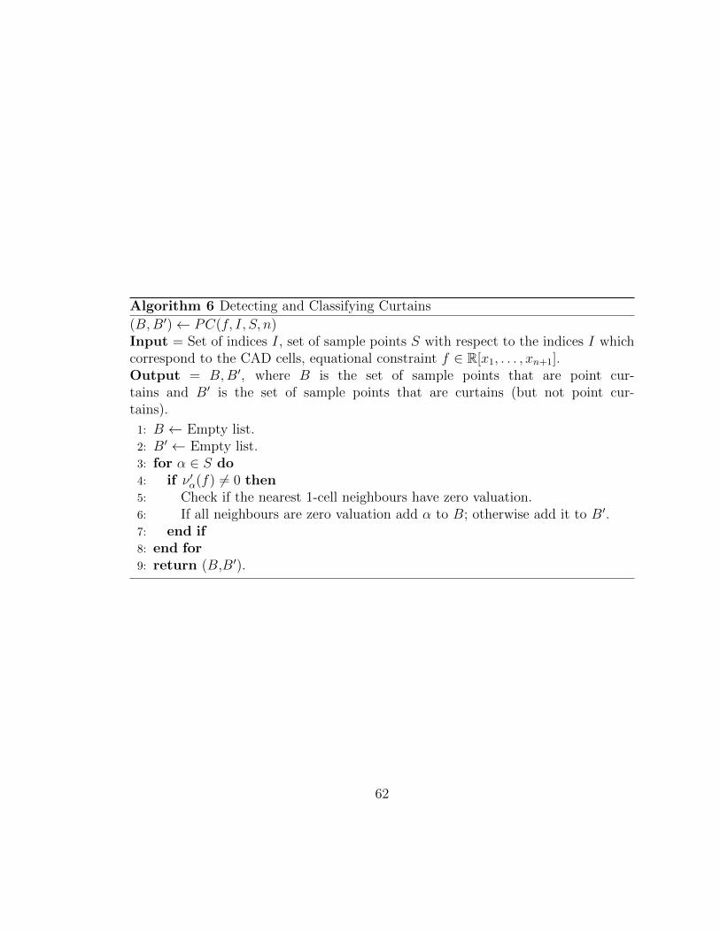
Algorithm 6 Detecting and Classifying Curtains

(B,B′)← PC(f, I, S, n)Input = Set of indices I, set of sample points S with respect to the indices I whichcorrespond to the CAD cells, equational constraint f ∈ R[x1, . . . , xn+1].Output = B,B′, where B is the set of sample points that are point cur-tains and B′ is the set of sample points that are curtains (but not point cur-tains).

1: B ← Empty list.2: B′ ← Empty list.3: for α ∈ S do4: if ν ′α(f) 6= 0 then5: Check if the nearest 1-cell neighbours have zero valuation.6: If all neighbours are zero valuation add α to B; otherwise add it to B′.7: end if8: end for9: return (B,B′).

62

Chapter 6

Further Developments ofEquational Constraints andCurtains

This chapter addresses the problem of curtains encountered in Chapter 4. Ourwork on single equational constraints in Chapter 4 and [NDS19] reduces the Lazardprojection by decomposing the hypersurface described by the equational constraint.In doing so, we only obtain information about the non-equational constraints fromtheir resultants with the equational constraint. As mentioned in Chapter 4, theseresultants give us no information on how the non-equational constraints interactwith each other on curtains of the equational constraint. In this chapter, we discusswhy point curtains do not cause Algorithm 5, which exploits a single hypersurface, tofail. We extend this by providing a subroutine that decomposes curtains of equationalconstraints.

The second half of this chapter looks at exploiting multiple hypersurfaces describedby equational constraints. The main idea is based on obtaining a solution space fora QFF of the shape

(f1 = 0) ∧ . . . ∧ (fk = 0) ∧ (. . .) (6.1)

using CAD algorithms. Since the QFF contains equational constraints f1, . . . , fk, anycell (in any CAD of Rn) that is a solution to the QFF would also be contained in thethe intersections of of Vf1 , . . . , Vfk . Hence we restrict our algorithm to decomposition

63

of the intersections of the equational constraints rather than the whole of Rn. The keydifference between this result and our result from Chapter 4 is that here we lift lex-least invariance to lex-least invariance rather than sign invariance. This enables us touse our projection operator recursively and takes advantage of multiple equationalconstraints. The specification of this is described in Section 6.2. Although thisresearch mimics [McC01], it builds on [MPP19], and hence we do not encounter thesame difficulties with curtains that arise in [McC01].

However, this algorithm, like the one from Chapter 4, fails when our equationalconstraints contain non-point curtains. To solve this problem, we could apply themethod from Section 6.1, but this would significantly increase the computationalcomplexity. This is further described in Chapter 9 along with the potential avenuesto deal with this problem.

6.1 Curtains on Single Hypersurfaces

This section introduces a subroutine that is executed when an equational constraintcontains a curtain. Our method is based on the fact that we can detect curtainsduring the lifting process of Algorithm 5 in Chapter 4. The subroutine is called ifand only if there are curtains detected.

Theorem 19 lifts lex-least invariance to sign invariance when the equational constraintdoes not contain a curtain. So far little work has been done on how the structureof CAD algorithms affect the decomposition of curtains. In the following section wedescribe how our work from Chapter 4 does decompose curtains of a certain type.

6.1.1 Point Curtains

The following theorems describe how point curtains do not pose a problem to Algo-rithm 5, because of the way cells are lifted.

Proposition 6. Let f, g ∈ R[x1, . . . , xn] and α ∈ Rn−1 and suppose that the varietyVf defined by f contains a curtain at α. Then Vg contains a curtain at α or intersectsVf at finitely many points over α.

This is the triviality that the intersection of Vf and Vg over α is either finite orinfinite, rewritten in terms of curtains.

The modified projection operator PLE(A) only projects information about the equa-tional constraint and the resultants between the equational and non-equational con-

64

straints.

Theorem 20. Let f, g ∈ R[x1, . . . , xn] and suppose that α ∈ Rn−1 is a point cellobtained from Algorithm 5. Suppose that f is an equational constraint and that Vfhas a point curtain at α. Then g is sign invariant in the sections and sectors of fαgα.

Proof. By assumption Vf has a point curtain at α. This implies that there existsa neighbourhood B of α in Rn−1 such that ν ′β(f) = 0n−1 for β ∈ B \ {α} andν ′α(f) 6= 0n−1. Because we are using the projection operator PLE, where E is the setof irreducible factors of f , the polynomial f is lex-least invariant with respect to theCAD produced by the projection operator PLE. Since the polynomial f is lex-leastinvariant with respect to the CAD and Vf has a curtain at α, the CAD consists ofcells of the form α× (a, b) or point cells α× {c}, where a, b, c ∈ R.

We know that res(f, g)(α) = 0. Then by Proposition 6, Vg has a point curtain atα or intersects Vf at finitely many points. If Vg has a curtain at α then g is signinvariant in all cells over α. Suppose Vf only intersects Vg at finitely many pointsand let A = {β1, . . . , βk} (arranged in increasing order) be the roots of fαgα. Thenthe cells above α will be of the form α×(a, b) or point cells α×{c}, where a, b, c ∈ A.Note that βi has to be either a root of fα or gα for each i. Since g = 0 intersectsf = 0 at only finitely many points and all roots of gα are in A, g is non-zero inα × (βi, βi+1). Otherwise g is zero on the point cells (α, βi) where βi is a root of g,and non-zero otherwise.

Curtains do not cause the algorithm in [Laz94] to halt. Hence in [Laz94] there was noneed for a result analogous to Theorem 20. However, as described in Chapter 4 andChapter 5, curtains pose a different problem when exploiting equational constraints,hence the need for Theorem 20.

6.1.2 Decomposing Curtain Base Set

Since we will be constantly referring to an arbitrary coordinate of a given point inthe following sections, we define the following function.

Definition 47. Let α = (α1, . . . , αn) ∈ Rn. We define CPROJk(α) to be the kth

coordinate of α, which is αk.

To understand our approach, we will first demonstrate it through a rough diagram ofthe main algorithm and an example. We further discuss this subroutine by providinga theorem that validates its use, followed by a standard algorithm.

65

Input Polynomial Constraints

Project to n− 1 using PLE

Project to first variable using PL recursively

Lift cells to n− 1-level ?

Check for curtains

Project NEC to 1 variable, using PL recursively

Yes

Lift to n− 1 level, only restricted to the curtains of EC

Add these sample points obtained in ?

Lift all cells to n-level

No

Sign-invariant CAD of single EC wrto the input polynomials

Figure 6-1: Flow chart describing our approach to decompose the variety describedby a single equational constraint

66

CAD

S1 S2 S3

S3,1 S3,2 S3,3 S3,4 S3,5

S4 S5 x1

x2

Figure 6-2: Set of sample points before Algorithm 7

CAD

S2 S2.1 S2.2 S2.3 S3

S3,2 S3,2.1 S3,2.2 S3,3 S3,3.1 S3,3.2 S3,4

S3.1 S3.2 S3.3 S4 x1

x2

Figure 6-3: Set of sample points after Algorithm 7

Consider a QFF having a set of polynomial constraints A in R[x1, x2, x3] with a singleequational constraint f . We start by projecting to x2 using the modified operatorPLE and then to x1 using the standard Lazard operator PL. We then lift to cells inR2. Figure 6-2 describes the tree structure of the cells obtained.

We have omitted some of the branches from the diagram to make it clearer. In Fig-ure 6-2 we have S1 < . . . < S5 and CPROJ2(S3,1) < . . . < CPROJ2(S3,5). Similarlywe have assumed the same ordering for Figure 6-3.

We proceed by checking if the sample points at the x2-level describe cells that arepart of the base of a non-point curtain in the equational constraint. This is firstdone by computing the roots in the range of neighbours of the curtain, and then bycomputing the sample points in the range of neighbours of the curtain. In our case,we assume that there is a non-point curtain at sample point S3,3. This sample ishighlighted in blue. We now project all the non-equational constraints to x1 usingonly the original Lazard operator PL. When lifting, we limit the sample points tothe curtain cells, as seen in Figure 6-3.

The final step combines the sample points from Figure 6-2 and the new sample points

67

showing in Figure 6-3 and lifts the cells to R3.

To decompose a curtain of an equational constraint is the same as decomposing a setS × R where S ⊂ Rn−1. When working in a curtain, the equational constraint doesnot give us any information on how the rest of the polynomial constraints interact.The following theorem validates our method of decomposing curtains separately.

Theorem 21. Let A = {f, g1, . . . gm} be a set of polynomial constraints where f isthe equational constraint. Let D be the CAD obtained using Algorithm 8. Then theconstraints g1, . . . , gm are sign invariant in the cells of D.

Proof. Let S be a connected subset of Rn−1 such that f is Lazard delineable overS and the set {res(f, gj)|1 ≤ j ≤ m} is lex-least invariant over S. If Vf does notcontain a non-point curtain on S, then by Theorem 19 and Theorem 20 we are done.Let us assume the contrary. Since Vf contains a non-point curtain on S, Algorithm 7splits up S into connected, non-intersecting subsets, where f is Lazard delineable andPL(g1, . . . , gm) is lex-least invariant. Hence by Theorem 17, g1, . . . , gm are lex-leastinvariant in the cells of the curtains of Vf , hence also sign invariant.

In Algorithm 7, the main parts are steps 3–7 and 14–18. For each recursion welook at the adjacent neighbours of the sample point describing the curtain. Wecompute the sample points within the neighbours of the curtains. In summary, weare restricting the computation of roots by using the neighbours of sample pointsdescribing curtains as boundaries.

68

Algorithm 7 Decomposing Curtain Base Set

(IC , SC)← DCBS(A, I, S, C,m)Input = A a set of polynomials in m variables. Set of sample points S and theirrespective indices I. The set of sample points describing the curtain base C ⊂ S.Output = SC is a set of sample points that decompose the base of curtainsdescribed by C and their respective indices IC .

1: If m ≥ 2 then go to step 9.2: for each c ∈ C do3: Let i = (i1, . . . , in) ∈ I be the index of c.4: Set (c1, c2)← Sample of indices (i1 − 1, 1 . . . , 1) and (i1 + 1, 1 . . . , 1).5: Isolate the real roots of all the irreducible factors of the elements of A between

the neighbours of CPROJ1(c1) and CPROJ1(c2).6: Construct cell indices and sample points for Lazard sections and sectors of

elements of A from i, α and the isolated real roots obtained from the previousstep.

7: Add the sample points to IC and SC .8: end for Exit.9: B ← the square free basis of the primitive parts of all elements of A.

10: P ← cont(A) ∪ PL(B).11: (I ′′, S ′′)← DCBS(P, I, S, C,m− 1).12: If m = n, set (IC , SC)← (I ′′, S ′′); return (IC , SC).13: (I ′, S ′)← (empty list,empty list).14: for each α ∈ S ′′ do15: f ∗ ← {fα | f ∈ B}.16: for each c ∈ C do17: Let i = (i1, . . . , in) ∈ I be the index of c.18: Set (c1, c2) ← Sample points given by indices (i1, . . . , im − 1, 1 . . . , 1) and

(i1, . . . , im + 1, 1 . . . , 1)19: Isolate the real roots of all the polynomials in f ∗ between the neighbours of

CPROJm(c1) and CPROJm(c2).20: Construct cell indices and sample points for Lazard sections and sectors

of elements of B from i, α and the isolated real roots obtained from theprevious step.

21: Add the sample points to IC and SC .22: end for23: end for24: return (IC , SC)

69

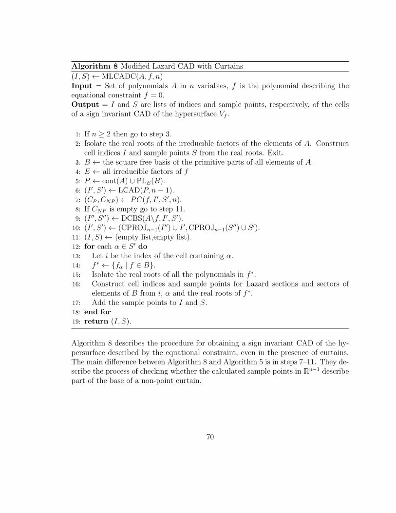
Algorithm 8 Modified Lazard CAD with Curtains

(I, S)← MLCADC(A, f, n)Input = Set of polynomials A in n variables, f is the polynomial describing theequational constraint f = 0.Output = I and S are lists of indices and sample points, respectively, of the cellsof a sign invariant CAD of the hypersurface Vf .

1: If n ≥ 2 then go to step 3.2: Isolate the real roots of the irreducible factors of the elements of A. Construct

cell indices I and sample points S from the real roots. Exit.3: B ← the square free basis of the primitive parts of all elements of A.4: E ← all irreducible factors of f5: P ← cont(A) ∪ PLE(B).6: (I ′, S ′)← LCAD(P, n− 1).7: (CP , CNP )← PC(f, I ′, S ′, n).8: If CNP is empty go to step 11.9: (I ′′, S ′′)← DCBS(A\f, I ′, S ′).

10: (I ′, S ′)← (CPROJn−1(I′′) ∪ I ′,CPROJn−1(S

′′) ∪ S ′).11: (I, S)← (empty list,empty list).12: for each α ∈ S ′ do13: Let i be the index of the cell containing α.14: f ∗ ← {fα | f ∈ B}.15: Isolate the real roots of all the polynomials in f ∗.16: Construct cell indices and sample points for Lazard sections and sectors of

elements of B from i, α and the real roots of f ∗.17: Add the sample points to I and S.18: end for19: return (I, S).

Algorithm 8 describes the procedure for obtaining a sign invariant CAD of the hy-persurface described by the equational constraint, even in the presence of curtains.The main difference between Algorithm 8 and Algorithm 5 is in steps 7–11. They de-scribe the process of checking whether the calculated sample points in Rn−1 describepart of the base of a non-point curtain.

70

One of the main questions in choosing a CAD algorithm that exploits equationalconstraints is the trade-off of time vs the quality of the decomposition. Lazard[Laz94] produces a lex-least invariant CAD of Rn: by contrast, our result produces asign invariant CAD of the hypersurface described by the equational constraint. If weonly wanted a sign invariant decomposition of the solution space, our approach wouldbe more efficient. On the other hand, if a full decomposition of Rn were needed, ourmethod would fall short. The algorithm described in this section decomposes curtainsof the equational constraint, hence improving the quality of the CAD as comparedto the approach of Chapter 4. However, it is computationally more expensive. Thiscomparison is further discussed in Chapter 8.

6.2 Multiple Hypersurfaces

The content of this section is analogous to what we did in Chapter 4. We modifyLazard’s projection operator and method to take advantage of multiple equationalconstraints in the input QFF. Let us recall what we mean by multiple equationalconstraints in a QFF:

(f1 = 0) ∧ . . . ∧ (fk = 0) ∧ (. . .).

In this QFF, the equational constraints are given by the polynomials f1, . . . , fk.Since a solution cell to the QFF must satisfy the equational constraints, we focusour attention on the intersection of equational constraints. First, let us define theprojection operator.

Definition 48. Let A be a finite set of irreducible polynomials in R[x1, . . . , xn] withn ≥ 2 and let E be a subset of A. The modified Lazard projection operator formultiple equational constraints PL∗E(A) is the subset of R[x1, . . . , xn−1] consisting ofthe following polynomials.

• All leading coefficients of the elements of A.

• All trailing coefficients of the elements of A.

• All discriminants of the elements of A.

• All resultants resxn(f, g), where f ∈ E and g ∈ A and f 6= g.

The way we take advantage of multiple equational constraints is by using this op-erator recursively. The resultants between the chosen equational constraint and the

71

A : a set of polynomialconstraints in n variables

EC : set of equational

constraints for A

f : select an equational

constraint from EC

EC ′ : set of equational

constraints for projection,

{resxn(f, f ′) | f ′ ∈ EC \ f}

B : square

free basis of A

E : elements from Bthat correspond to f

PL∗E(B) : the projection ofthe polynomial constraints A

remaining equational constraints are equational constraints of the projected poly-nomials. Hence we take the equational constraints one at a time, so if we have kequational constraints we will use PL∗E(A) for the first k projections. The followingtheorems validate the use of PL∗E(A) recursively.

Theorem 22. Suppose f, g ∈ R[x1, . . . , xn] both have positive degree in xn, and thatf, g are not identically zero. Let S ⊂ Rn−1 be a connected subset such that f doesnot have a curtain over S. If discxn(g), ldcfxn(g), trcfxn(g) and resxn(f, g) are alllex-least invariant over S, then g is lex-least invariant on every section and sector off over S.

Proof. From Theorem 18 we know that g is sign invariant in the sections of f . Sincediscxn(g), ldcfxn(g) and trcfxn(g) are lex-least invariant over S, g is Lazard delineableover S from Theorem 16. Hence g is lex-least invariant in the sections and sectorsof f .

Theorem 23. Let A be a set of pairwise relatively prime irreducible polynomials inn variables x1, . . . , xn of positive degrees in xn, where n ≥ 2, and let E be a subsetof A. Let S be a connected subset of Rn−1. Suppose that each element of PL∗E(A)is lex-least invariant in S. Then each element of E is Lazard delineable over S andexactly one of the following is true.

1. The hypersurface defined by the product of the elements of E has a curtain

72

over S. Each element of A \ E is lex-least invariant in the intersection withthe curtain.

2. The Lazard sections of the elements of E are pairwise disjoint over S. Eachelement of A is lex-least invariant in such Lazard sections.

Proof. The resultants are only needed to split cells that are contained in the sectorsof f ∈ E or the curtains of f ∈ E. From Theorem 22 we know that each elementof A \ E is lex-least invariant on every section of f ∈ E independently. Since eachelement of resxn(E,A \E) is invariant on S, it follows that each element of A \E islex-least invariant on all sections of f ∈ E simultaneously.

The difference between the projection operators PLE(A) and PL∗E(A) is that PLE(A)does not consider the leading coefficients, trailing coefficients and the discriminantsof the non-equational constraints. The method using a single equational constraintis significantly more efficient than Lazard’s original method with respect to timeand space complexity (see Section 8.2). However, that need not be the case whencomparing the multiple equational constraint approach to the single equational con-straint approach. That is because it is dependent on the number of constraints inQFF, the number of irreducible factors, the number of variables etc. This is furtherdiscussed in Chapter 8.

The usage of the projection operator PL∗E(A) has been described in Algorithm 9.Steps 4–7 describe choosing an equational constraint and using the operator PL∗E(A).Step 9 is only called if there are equational constraints left to exploit.

Theorem 20 can be extended to show that the non-equational constraints are lex-leastinvariant on a point curtain of an equational constraint.

Corollary 3. Let f, g ∈ R[x1, . . . , xn] and α ∈ Rn−1. Suppose that f is an equationalconstraint and Vf has a point curtain at α. Then g is lex-least invariant in thesections and sectors of fg over α.

Proof. The proof follows directly from above, with minor changes when g has acurtain at α. Since α is a point in Rn−1, g is Lazard delineable over α. Thus everyLazard section of fg over α is contained within a Lazard section of g. Furthermore,every Lazard sector of fg over α is either a Lazard sector of f or a Lazard sector ofg. Hence g is lex-least invariant in every Lazard section and sector of fg over α.

73

Algorithm 9 Modified Lazard CAD Multiple Equational Constraints

(I, S)← MLCADME(A,E, n)Input = Set of polynomials A in n variables and a set of polynomials describing theequational constraints E.Output = I and S are lists of indices and sample points, respectively, of the cellscomprising a lex-least invariant CAD of the intersections of the hypersurfaces de-scribed by the elements of E.

1: If n ≥ 2 then go to step 3.2: Isolate the real roots of the irreducible factors of the non-zero elements of A.

Construct cell indices I and sample points S from the real roots. Exit.3: B ← the square free basis of the primitive parts of all elements of A.4: f ← Select an equational constraint from E.5: E ← all irreducible factors of f .6: E ′ ← {resxn(f, f ′) | f ′ ∈ E\{f}}.7: P ← cont(A) ∪ PL∗E(B).8: If E ′ is empty go to step 11 else go to step 9.9: (I ′, S ′)← MLCADME(P,E ′, n− 1).

10: Go to step 12.11: (I ′, S ′)← LCAD(P, n− 1).12: (I, S)← (empty list,empty list).13: for each α ∈ S ′ do14: Let i be the index of the cell containing α.15: f ∗ ← {fα | f ∈ B}.16: Isolate the real roots of all the polynomials in f ∗.17: Construct cell indices and sample points for Lazard sections and sectors of

elements of B from i, α and the real roots of f ∗.18: Add the sample points to I and S.19: end for20: return (I, S).

74

Corollary 4. Let f, g1, . . . , gm ∈ R[x1, . . . , xn] and α ∈ Rn−1. Suppose that f is anequational constraint and Vf has a point curtain at α. Then g1, . . . , gm are lex-leastinvariant in the sections and sectors of fg1 . . . gm over α.

Proof. Let us consider the case m = 2. From Corollary 3 we know that f and g1 arelex-least invariant on sections of fg1. Applying the same Corollary to fg1 and g2,we get that fg1 and g2 are lex-least invariant on every section and sector of fg1g2.Hence, f , g1 and g2 are lex-least invariant in every Lazard section and sector of fg1g2over α. The result follows by trivial induction.

Corollary 5. Let A ⊂ R[x1, . . . , xn] be a set of irreducible polynomials and let E ⊂A. Let S be a connected subset of Rn−1 such that every element of PL∗E(A) is lex-leastinvariant in S. Then each element of E either vanishes identically on S or is Lazarddelineable on S. If S is a point, then all elements of A \E are lex-least invariant inthe Lazard sections and Lazard sectors of f . If S is not a point, then the sectionsof any f ∈ E that does not vanish identically over S are pairwise disjoint, and eachelement of A \ E is lex-least invariant in every such section.

Proof. This is a direct consequence of Corollary 4 and Theorem 23.

6.3 Summary

Rewriting the problem of nullification using curtains has given us a better under-standing of why our modifications to Lazard’s work fails in the presence of curtains.We have used this knowledge to provide a subroutine that circumvents the problemscaused by curtains. In doing so, we established that point curtains do not causeproblems in our modifications of Lazard’s algorithm. We have also described analgorithm that can take advantage of multiple equational constraints in a QFF.

In the next chapter, we adapt our algorithms from Chapters 4–6 to the recent devel-opments made by Brown and McCallum in [BM20].

75

Chapter 7

Brown-McCallum Projection

Towards the end of 2020, Brown and McCallum defined a modified version of Lazard’sprojection operator that allows one to omit the trailing coefficients of the polynomialconstraints under certain circumstances. In summary, they propose that if a poly-nomial constraint has only finitely many point curtains, one can omit the trailingcoefficient in the projection set.

They do still use the notion of nullification, which we have translated to the termi-nology of curtains. The notations of [BM20] match those of [MPP19] but here wehave used the same notation and terminology that is used elsewhere in this thesis.Most of the results presented in this chapter are a direct consequence of the theoremsstated in Chapter 4 and Chapter 6.

7.1 Brown-McCallum Modification

In Chapter 6 we handle curtains in equational constraints and we detect the curtainswhen lifting. However, Brown and McCallum’s improvement [BM20] is to omit thetrailing coefficients of a polynomial constraint if we know that it has no curtains orfinitely many point curtains. This obliges them to detect curtains in the projectionphase instead. Hence our work on detecting curtains is not appropriate for their use.

We define a procedure T that takes as input a polynomial constraint f ∈ R[x1, . . . , xn]and outputs either a set S ⊂ Rn−1 or FAIL. The requirement for T is that if it returnsa set S, then S must be finite and must contain all the points at which f has a curtain.

There are various ways one could approach this. A simple way would be to show

76

that the system of equations defined by the coefficients of f (in variables x1, . . . , xn)is unsatisfiable over the reals. This can be achieved using several methods: an easyway would be to use linear substitution. If such a test fails, then we resort to anysuitable finite zero-test over C. If the tests mentioned above fail, T returns FAIL.If one of the tests discussed above succeeds, then T computes a suitable finite setS ⊂ Rn−1.

The following defines the Brown-McCallum projection operator, which uses the pro-cedure T to determine which polynomials’ trailing coefficients can be omitted. TheBrown-McCallum operator also depends on a set of points Γ, which is a list of pointsthat track the bases of point curtains through the projection phase. When Algo-rithm 10 is first called, Γ is initialised to the empty set.

Definition 49. [BM20, Definition 4] Let A ⊂ R[x1, . . . , xn] be a finite irreduciblebasis, with n ≥ 2. Let Γ be a finite set of points in Rn. The Brown-McCallumoperator BM(A,Γ) is a finite subset of R[x1, . . . , xn−1] consisting of the followingpolynomials:

• All leading coefficients of the elements of A

• All discriminants of the elements of A

• All resultants of distinct pairs of elements of A

• All trailing coefficients (i.e. coefficients independent of xn) of the elements ofA for which T returns FAIL.

together with the set of points

{(γ1, . . . , γn−1) | (γ1, . . . , γn) ∈ Γ)} ∪⋃f∈A

T (f),

where A = {f | f ∈ A ∧ T (f) 6= FAIL}

The following theorem justifies the use of the projection operator BM(A,Γ).

Theorem 24. [BM20, Theorem 3] Let f be a polynomial in R[x1, . . . , xn] with posi-tive degree in xn and let S be a connected subset of Rn−1. Suppose that the discrim-inant and leading coefficient of f are lex-least invariant in S and f has no curtainover S. Then f is Lazard delineable over S, hence lex-least invariant in every Lazardsection and sector.

Theorem 24 states that we are allowed to use the projection operator BM if f doesnot contain a curtain. However, the method used by Brown and McCallum in [BM20]

77

is similar to ours in Theorem 20. The idea stems from the structure of lifting and thefact that it is easy to identify point curtains. In summary, the base of point curtainsof an input polynomial at n-level will be a point cell in the (n− 1)-level.

Algorithm 10 Brown-McCallum algorithm for lex-least invariant CAD

(I, S)← BMCADL(A)Input = Set of polynomials A in n variables and Γ a set of points in Rn.Output = I and S are lists of indices and sample points, respectively, of the of alex-least invariant CAD of A.

1: If n ≥ 2 then go to step 3.2: Isolate the real roots of the irreducible factors of the non-zero elements of A.

Construct cell indices I and sample points S from the real roots and the pointsin Γ. Exit.

3: B ← the squarefree basis of the primitive parts of all elements of A.4: (P,Γ′)← BM(B, ∅).5: (I ′, S ′)← BMCADL(cont(A) ∪ P,Γ′).6: (I, S)← (empty list,empty list).7: for each α ∈ S ′ do8: Let i be the index of the cell containing α.9: f ∗ ← {fα | f ∈ B}.

10: Let D be the isolated real roots of f ∗.11: Set E ← {γn | (α1, . . . , αn−1, γn) ∈ Γ}.12: Construct cell indices and sample points for Lazard sections and sectors of

elements of B from i, α and D ∪ E.13: Add the sample points to I and S.14: end for15: return (I, S)

Theorem 25. Let A = {f1, . . . , fm} be a set of pairwise relatively prime irreduciblepolynomials in n variables x1, ..., xn of positive degrees in xn, where n ≥ 2. Let Γbe a finite set of points in Rn. Let S be a subset of Rn−1 obtained via Algorithm 4and suppose that each element of BM(A,Γ) is lex-least invariant in S. Then everyelement of A is lex-least invariant in the Lazard sections and sectors of every otherelement.

Proof. The proof is similar to the proof of Theorem 17 and is a direct consequenceof Thorem 24.

78

7.2 Brown-McCallum Projection with Equational

Constraints

In [BM20], the authors state that their projection operator should be compatiblewith the single and multiple equational constraint versions of the Lazard projectionoperator. In this section we provide the modified versions of the Brown-McCallumprojection operator, such that it can be used for single and multiple equationalconstraint cases.

7.2.1 Single Equational Constraint

The modified version for Brown-McCallum projection operator is not readily trans-latable from Lazard’s version. This is because the Brown-McCallum projection op-erator needs as input a set Γ of points that describe point curtains in a polynomialconstraint.

Definition 50. Let A be a finite irreducible basis in R[x1, . . . , xn], with n ≥ 2.Let Γ be a finite set of points in Rn and E ⊂ A. The modified Brown-McCallumprojection operator BME(A,Γ) is a finite subset of R[x1, . . . , xn−1] containing thefollowing polynomials:

• All leading coefficients of the elements of E;

• All discriminants of the elements of E;

• All resultants resxn(f, g) for all f ∈ E, g ∈ A and f 6= g;

• All trailing coefficients of the elements of E for which T returns FAIL;

together with the points

{(γ1, . . . , γn−1) | (γ1, . . . , γn) ∈ Γ} ∪⋃f∈E

T (f)

where E = {f | f ∈ E ∧ T (f) 6= FAIL}.

Theorem 26. Let A be a set of pairwise relatively prime irreducible polynomials inn variables x1, ..., xn of positive degrees in xn, where n ≥ 2. Let E be a subset of Aand let Γ be a finite set of points in Rn. Let S be a connected subset of Rn−1. Supposethat each element of BME(A,Γ) is lex-least invariant in S. Then each element of Eis Lazard delineable on S and exactly one of the following must be true.

79

1. The hypersurface defined by the product of the elements of E has a curtainover S.

2. The Lazard sections over S of the elements of E are pairwise disjoint. Eachelement of E is lex-least invariant in every such Lazard section. Each elementof A \ E is sign invariant in every such Lazard section.

Proof. In Theorem 18, we require f to be Lazard delineable over a connected subsetS without specifying how S is obtained. We can use the projection operator BM todo so. Similarly the only other requirement is that resxn(f, g) is lex-least invariantover S. Therefore we can use BME. Hence from Theorem 19 and Theorem 25 theresult follows.

In Theorem 18, we are not concerned with the projection operator used, rather weare concerned with which polynomials are lex-least invariant. Hence the Brown-McCallum projection operator can be used to obtain the lex-least invariance statedin the assumptions of the theorem. This shows that modifying a projection operatorto use it for single equational constraints is possible irrespective of the projectionoperator being used. This is further discussed in Chapter 9.

7.2.2 Multiple Equational Constraints

In this section we present the modified version of the Brown-McCallum projectionoperator for the multiple equational constraint case. This is a direct consequence ofthe results in Section 6.2.

Definition 51. Let A be a finite irreducible basis in R[x1, . . . , xn], with n ≥ 2. LetΓ be a finite set of points in Rn and let E ⊂ A. The modified Brown-McCallumprojection operator BM∗E(A,Γ) is a finite subset of R[x1, . . . , xn−1] containing thefollowing polynomials:

• All leading coefficients of the elements of A;

• All discriminants of the elements of A;

• All resultants resxn(f, g) for all f ∈ E, g ∈ A and f 6= g;

• All trailing coefficients of the elements of A for which T returns FAIL;

80

Algorithm 11 Brown-McCallum modified algorithm for sign invariant CAD

(I, S)← BMCADS(A, f,Γ, n)Input = Set of polynomials A in n variables, Γ a set of points in Rn and f thepolynomial describing the equational constraint f = 0.Output = I and S are lists of indices and sample points, respectively, of the cellsof a sign invariant CAD of the hypersurface Vf .

1: If n ≥ 2, then go to step 3:2: Isolate the real roots of the irreducible factors of the non-zero elements of A.

Construct cell indices I and sample points S from the real roots and the pointsin Γ. Exit.

3: B ← the squarefree basis of the primitive parts of all elements of A.4: E ← all irreducible factors of f from B5: (P,Γ′)← BME(B,Γ).6: (I ′, S ′)← BMCADL(P, n− 1).7: (I, S)← (empty list,empty list).8: for each α ∈ S ′ do9: Let i be the index of the cell containing α.

10: f ∗ ← {fα | f ∈ B}.11: Let D be the isolated real roots of f ∗.12: Set E ← {γn | (α1, . . . , αn−1, γn) ∈ Γ}.13: Construct cell indices and sample points for Lazard sections and sectors of

elements of B from i, α and D ∪ E.14: Add the sample points to I and S.15: end for16: return (I, S)

together with the points

{(γ1, . . . , γn−1) | (γ1, . . . , γn) ∈ Γ}⋃f∈A

T (f)

where A = {f | f ∈ A ∧ T (f) 6= FAIL}.

Theorem 27. Let A be a set of pairwise relatively prime irreducible polynomials inn variables x1, . . . , xn of positive degrees in xn, where n ≥ 2. Let E be a subset of Aand let Γ be a finite set of points in Rn. Let S be a connected subset of Rn−1. Supposethat each element of BM∗E(A,Γ) is lex-least invariant in S. Then each element of Eis Lazard delineable over S and exactly one of the following is true.

81

1. The hypersurface defined by the product of the elements of E has a curtainover S. Each element of A \ E is lex-least invariant in the intersection withthe curtain.

2. The Lazard sections of the elements of E are pairwise disjoint over S. Eachelement of A is lex-least invariant in such Lazard sections.

Proof. This proof follows a similar argument to the proof of Theorem 26. The resultfollows from Theorem 25 and Theorem 23.

7.3 Summary

We present our modified verisons of the Brown-McCallum operator for the single andmultiple equational constraint case. Throughout Chapter 4 to Chapter 7, we focuson the algorithms used to produce a CAD rather than the valuation used, in ourcase the lex-least valuation. We discuss this further in the conclusion of this thesis,as a potential avenue to continue the research presented here.

82

Algorithm 12 Modified Brown-McCallum CAD for Multiple Equational Con-straints(I, S)← BMCME(A,Γ, E, n)Input = Set of polynomials A in n variables, Γ a set of points in Rn,E a set of polynomials describing the equational constraints.Output = I and S are lists of indices and sample points, respectively, of the cellsof a lex-least invariant CAD of the intersections of the hypersurface described bythe elements of E.

1: If n ≥ 2 then go to step 3.2: Isolate the real roots of the irreducible factors of the non-zero elements of A.

Construct cell indices I and sample points S from the real roots and the pointsin Γ. Exit.

3: B ← the squarefree basis of the primitive parts of all elements of A.4: f ← Select an equational constraint from E.5: F ← all irreducible factors of f .6: E ′ ← {resxn(f, f ′) | f ′ ∈ E\{f}}.7: (P,Γ′)← BM∗F (B,Γ).8: If E ′ is empty go to step 11 else go to step 9.9: (I ′, S ′)← BMCME(P,Γ′, E ′, n− 1).

10: Go to step 12.11: (I ′, S ′)← BMCADL(P,Γ′, n− 1).12: (I, S)← (empty list,empty list).13: for each α ∈ S ′ do14: Let i be the index of the cell containing α.15: f ∗ ← {fα | f ∈ B}.16: Let D be the isolated real roots of f ∗.17: Set E ← {γn | (α1, . . . , αn−1, γn) ∈ Γ}.18: Construct cell indices and sample points for Lazard sections and sectors of

elements of B from i, α and D ∪ E.19: Add the sample points to I and S.20: end for21: return (I, S).

83

Chapter 8

Complexity Analysis

In this thesis we have provided various improvements to the original algorithmsproposed by Lazard [Laz94] and Brown-McCallum [BM20], influenced by [McC99]and [McC01]. This chapter provides a comprehensive complexity analysis of themethods presented in this thesis. Our measure of calculating the complexity ofalgorithms is the number of cells that a CAD algorithm produces, rather than its timecomplexity. A variety of previously conducted experiments show a strong correlationbetween the number of cells computed by a CAD algorithm and computation time[BDE+16]. For each algorithm we compute the dominant term in the cell countbound.

We focus on three parameters when conducting the complexity analysis: the numberof variables n, the number of polynomials m and the maximum degree d (in any onevariable). We first recall terminology used in this chapter.

Definition 52. Let {fi} be a finite set of polynomials. The combined maximumdegree of {fi} is the maximum element of the set⋃

j

{degxj(∏i

fi)}.

For example, the set {x3 + y, x4 + y2} has combined degree 7 (in x), whereas the set{x3 + y6, x4 + y2} has combined degree 8 (in y). Note that the chosen main variableis irrelevant and we are only interested in the maximum possible degree.

Definition 53. [McC85, Section 6.1] A set of polynomials has the (m, d)-propertyif it can be partitioned into m sets, such that the combined maximum degree of each

84

set is less than or equal to d.

Example 14. The set of polynomials {x3 +y, x5 +y2, x5y+x3, x3 +y} has combinedmaximum degree 16 and thus the (1,16) - property. If we partition this set into foursets of one polynomial each, it also has the (4,5)-property. We can also split this setinto two sets, which would give us the (2,8), (2,10), (2,11) and (2,13)-properties.

In fact, it is not necessary to require a partition in Definition 53. Equivalently, a setA has the (m, d)-property if it can be decomposed as the union A = S1 ∪ . . . ∪ Smof possibly overlapping sets, such that the combined maximum degree of each set isless than or equal to d.

Proposition 7. [BDE+16, Proposition 8] If A is a set of polynomials with the (m, d)-property, then a squarefree basis of A will also have the (m, d)-property.

This can be easily seen, as a squarefree basis of A would only increase the numberof polynomials but will not increase the degree of their product.

Proposition 8. [BDE+16, Proposition 9] If A is a set of polynomials with the (m, d)-property, then A has the (dm

le, ld)-property.

This can also be seen easily, by grouping the subsets together, l at a time.

Referring back to Example 14, we see that the set of polynomials has the (2,8)-property and therefore also has the (1,16)-property, in which case l = 2. Let us focuson the (4,5)-property instead. If we take l = 3, from Proposition 8 we get that it hasthe (2, 15)-property, which we can see that it does. Indeed, it has the (2,13)-propertywhich according to Definition 54 is stronger.

The main idea behind the analysis is to find an upper bound on the number of rootsand then recursively compute the total number of cells being produced in the worstcase scenario. We start by analysing the complexity of the projection set.

When projecting with equational constraints we need to use an enhanced version ofthe (m, d)-property, so that any statement made about projection operators usingequational constraints can be used recursively.

Definition 54. Let A be a set of polynomial factors of a family of polynomial con-straints. We say that A has the (m, d)k-property if A can be written as the union ofm sets each of max combined degree ≤ d and each of the first k sets consist of thefactors of a single equational constraint.

This chapter is split into three sections, dedicated to the advancements made on Mc-Callum’s algorithm, Lazard’s algorithm and the Brown-McCallum algorithm. Within

85

each section we go through the complexity analysis of the original algorithm, fol-lowed by the single equational constraint variant and then the multiple equationalconstraint variant.

If it were the case that the combined maximum degree of all our polynomial con-straints were 1, then the system of equations describe a set of polytopes, which canbe solved more efficiently using algorithms other than CAD, see for instance [Kar84].Hence in all our results we make the assumption that the combined max degree d isgreater than 1.

8.1 Analysis of McCallum’s Projection Operators

Most of the results in this section have been taken from [BDE+16]. We use theanalysis presented here as a base for the analysis provided in the remainder of thechapter.

Proposition 9. [BDE+16, Lemma 11] If A is a set of polynomials with the (m, d)-property, then P(A) has the (M, 2d2)-property with

M =

⌊(m+ 1)2

2

⌋. (8.1)

Proof. Let A = S1∪ . . .∪Sm according to the (m, d)-property. Let B be a squarefreebasis of prim(A). Let T1 ⊆ B be the factors of S1 and let Ti ⊆ B be the factors ofSi that are not in Tj with j < i. Split P(A) as follows

P(A) = CA⋃{⋃

i

CAi

}⋃{⋃i<j

CAi,j

}

1. CA: All non-leading coefficients of B.

2. CAi: cont(Si) ∪ ldcf(Ti) ∪ disc(Ti) ∪ res(Ti).

3. CAi,j: res(Ti, Tj) with i 6= j.

By Lemma 3, the set of non-leading coefficients of Ti has the (1, d2)-property. SinceCA is the union of the set of non-leading coefficients for all possible Ti, CA has the(m, d2)-property. Using Proposition 8 we get that CA has the (dm/2e, 2d2)-property.

By Lemma 4, each CAi has the (1, 2d2)-property. There are m possible values for i,so ∪i CAi has the (m, 2d2)-property.

86

Fix i, j and consider res(∏

f∈Ti f,∏

g∈Tj g), which contains the product of all resul-

tants in res(Ti, Tj) by Equation 2.6. This is a resultant of two polynomials with atmost degree d, hence the resultant will have at most degree 2d2. Applying this to allpossible values for i, j, we get that ∪i<j CAi,j has the (1

2m(m− 1), 2d2)-property.

Combining all three we get P(A) has the (M, 2d2)-property where

m+m(m− 1)

2+⌈m

2

⌉≤ m(m+ 1)

2+

⌊m+ 1

2

⌋≤⌊

(m+ 1)2

2

⌋= M (8.2)

Lemma 3. Let Ti be as defined in Proposition 9. The set of all non-leading coeffi-cients of Ti has the (1, d)-property.

Proof. The product of all elements in Ti has at most degree d. This implies thatthe polynomials in Ti have at most d non-leading coefficients, each of whose degreeis at most d. This implies that the set of non-leading coefficients of Ti has the(1, d2)-property.

Lemma 4. The set CAi as defined in Proposition 9 has the (1, 2d2)-property.

Proof. Define c as the product of all elements in cont(Si). Suppose Ti = {F1, . . . , Ft}for some t and put F = cF1 . . . Ft. Thus, F divides the product of all elements in Siand has degree at most d (since A has the (m, d) property). Let F ′ be the derivativeof F with respect to xn. Since F has at most degree d, res(F, F ′) has degree at most2d2, since it is the determinant of a (2d− 1× 2d− 1) matrix. From Equation 2.4 weget that res(F, F ′) = c′ disc(F ) where c′ is a power of c. Applying Equation 2.5 oncegives us

disc(F ) = disc(Ft) disc(F1 . . . Ft−1) res(F1 . . . Ft−1, Ft)2. (8.3)

Applying Equation 2.6 to Equation 8.3 repeatedly gives

disc(F ) = disc(F1 . . . Ft−1) disc(Ft)t−1∏j=1

(res(Fj, Ft)2). (8.4)

Applying both Equation 2.6 and Equation 2.5 recursively we get that res(F, F ′) isthe product of a power of c and

(t∏

j=1

ldcf(Fj) disc(Fj))(∏

1≤i<j≤t

(res(Fi, Fj))2). (8.5)

87

Since this includes all elements of CAi we are done.

In order to get the complexity of the whole process of CAD we must apply thisrecursively. To make calculations easier we weaken the bound as follows.

Corollary 6. [McC85] If A is a set of polynomials with the (m, d)-property wherem > 1 then P (A) has the (m2, 2d2)-property.

When computing the upper bound on the number of cells we use the result fromProposition 9 for the first recursion and use Corollary 6 for the subsequent recursions.Table 8.1 describes the growth of the projected polynomials using P(A). Note thatcolumns in Table 8.1 do not refer to the number of polynomials and their degree,but to the number of sets and the max combined degree given by Definition 53. The

Table 8.1: Growth of polynomials in CAD

Variables Number mi Degree di Product midi

n m d mdn− 1 M 2d2 2Md2

n− 2 M2 8d4 23M2d4

n− 3 M4 128d8 27M4d8

......

......

n− r M2r−122r−1d2

r22r−1M2r−1

d2r

......

......

1 M2n−222n−1−1d2

n−122n−1−1M2n−2

d2n−1

Product M2n−1−1m 22n−1−nd2n−1 22n−1−nM2n−1−1md2

n−1

number of real roots of the projected polynomials determines the size of the CAD.We can bound the number of real roots of the univariate polynomials by the productof the elements in columns 2 and 3 of Table 8.1. The number of cells produced inR1 is twice this product plus 1. Hence the total number of cells in the CAD can begiven by the product of 2K + 1 where K varies through all the products betweencolumn 2 and 3 of Table 8.1, which is given by

(2md+ 1)n−1∏i=1

(2(22i−1M2i−1

d2i

) + 1). (8.6)

88

Since we are interested in the complexity, we can omit the ‘+1’ term in the productto give us the dominant term of the expression:

2mdn−1∏i=1

(2(22i−1M2i−1

d2i

)) = 22n−1M2n−1−1md2n−1. (8.7)

Substituting the value for M from Equation 8.2 we get the upper bound

22n−1(

(m+ 1)2

2

)2n−1−1

md2n−1 = 22n−1

(m+ 1)2n−2md2

n−1. (8.8)

This bound is doubly exponential with respect to n. Hence even a small jump fromn = 4 to n = 5 has a drastic effect on the time and space complexity of the algorithm.

8.1.1 Single Equational Constraint McCallum

Let us now consider McCallum’s modified projection operator PE(A) for the singleequational constraint case. Assuming there is an equational constraint, it is clearthat PE(A) ⊆ P(A) from their definitions. Since PE(A) is used only at the first levelwhen computing a CAD (i.e. when projecting from n to n− 1), we can use Table 8.1for our complexity calculations with a different value for M .

Theorem 28. Let A be a set of polynomial factors of a family of polynomial con-straints. Suppose that A has the (m, d)k-property with d ≥ 2 and k ≥ 1. Let E be thefirst set of the (m, d)k decomposition and let F be the squarefree basis of E. ThenPF (A) has the (M, 2d2)k′-property (with respect to the family of projected polynomialconstraints) where

M =

⌊5m+ 4

4

⌋(8.9)

and k′ < k.

Proof. Let A = S1 ∪ ... ∪ Sm according to the (m, d)k-property, so that E = S1 andS2, ..., Sk are associated with equational constraints. Since E has the (1, d)-property,its squarefree basis F has the (1, d)-property.

• From the proof of Proposition 9 we see that the set of leading coefficients,discriminants, resultants and contents of F form a set R1 which has the (1, 2d2)-property.

89

• By Lemma 3 the remaining coefficients of F form a set R2 which has the (1, d2)-property. Set R3 = cont(A) \ cont(E). Clearly R3 ⊆ cont(A \ E) and A \ Edecomposes into (m−1) sets each of max combined degree d. Hence the set R3

has the (m− 1, d)-property, thus the (⌈m−12

⌉, d2)-property. Then R2 ∪ R3 has

the (⌈m−12

⌉+ 1, d2)-property; hence by Proposition 8 the (

⌈dm−1

2 e+1,

2

⌉, 2d2)-

property. Hence we get that R2 ∪R3 has the (⌊m+3d−2

2d

⌋, 2d2)-property.

• From the proof of Proposition 9, res(Si, F ) has the (1, 2d2)-property for i > 1.Hence R4 =

⋃i>1 res(Si, F ) has the (m− 1, 2d2)-property.

Hence the set PF (A) = R1 ∪R2 ∪R3 ∪R4 has the (M, 2d2)-property where

1 +

⌊m+ 3d− 2

2d

⌋+ (m− 1) ≤

⌊5m+ 4

4

⌋= M. (8.10)

Moreover, the decomposition of R4 according to the (m−1, 2d2)-property is as givenabove, and the sets in the decomposition of PF (A) associated with a projected equa-tional constraint are precisely the nonzero res(Si, F ) for 1 < i ≤ k, so PF (A) has the(M, 2d2)′k-property for some k′ < k.

To obtain the dominant term on the cell bound we substitute the value from Theo-rem 28 in Equation 8.7 and get

22n−1(

5m+ 4

4

)2n−1−1

md2n−1 = 22n−1

(5m+ 4

2

)2n−1−1

md2n−1. (8.11)

Comparing the dominant terms given by Equation 8.8 and Equation 8.11, we seethat

(m+ 1)2 ≥ 5m+ 4

2(with m > 1), (8.12)

which implies that the complexity is reduced when using PE(A) instead of P(A).

8.1.2 Multiple Equational Constraint McCallum

In this section we analyse McCallum’s final modification for order invariant CADs,P∗E(A) for multiple equational constraints. In the process we also fill a gap in a proofin [EBD19].

90

Theorem 29. Let A be a set of polynomial factors of a family of polynomial con-straints. Suppose that A has the (m, d)k-property with d ≥ 2 and k ≥ 1. Let E be thefirst set of the (m, d)k decomposition and let F be the squarefree basis of E. ThenPF (A) has the (3m, 2d2)k′-property (with respect to the family of projected polynomialconstraints) where k′ < k.

Proof. From Theorem 28 we know that PF (A) decomposes into⌊5m+4

4

⌋sets, each

of maximum combined degree 2d2. Each set in the decomposition of A \ E has amax combined degree of d, hence will generate a discriminant of degree 2d(d − 1)and (d+ 1) coefficients of degree d. Taking the discriminant and leading coefficientstogether and all the non-leading coefficients together, we get two sets that have the(1, 2d2)-property and the (1, d2)-property respectively.

Since there are (m− 1) sets in the decomposition of A \ E, the set of discriminantsand leading coefficients has the (m − 1, 2d2)-property and the set of non-leadingcoefficients has the (m − 1, d2)-property, and by Proposition 8 the (dm−1

2e, 2d2)-

property. Hence the projection P∗F (A) has the (M, 2d2)-property where⌊5m+ 4

4

⌋+ (m− 1) +

⌈m− 1

2

⌉≤⌊

11m

4

⌋≤ 3m = M. (8.13)

There are k equational constraints, so Theorem 28 implies that P∗F (A) has the(M, 2d2)k′-property (with respect to the family of projected polynomial constraints)where k′ < k.

If there are l equational constraints, we can apply this result in the first l rows inTable 8.2. For the remaining rows we use Corollary 6.

The total number of cells in the CAD is given by the product of 2K + 1 where Kvaries through all the products between column 2 and 3 of the Table 8.2, and we get

n∏i=1

(2midi + 1) =

n−(l+1)∏i=1

(2midi + 1)×n∏

s=n−l

(2msds + 1). (8.14)

Since we are only concerned with the dominant term, we omit the ‘+1’ and get

n−(l+1)∏i=1

(2midi) =

n−(l+1)∏i=1

(32rlm2r22l+r−1d2l+r

) = 3lsn−1−2lm2n−l−2(2d)2

n−2l+1

(8.15)

n∏s=n−l

(2msds) =n∏

s=n−1

3sm22s−1d2s

= 3l(l+1)/2ml+1(2d)2l+1−1. (8.16)

91

Table 8.2: Growth of polynomials in CAD

Variables Number mi Degree di Product midi

n m d mdn− 1 3m 2d2 2 · 3md2

......

......

n− l 3lm 22l−1d2l

3lm22l−1d2l

n− (l + 1) 32lm2 22l+1−1d2l+1

32lm222l+1−1d2l+1

......

......

n− (l + r) 32rlm2r 22l+r−1d2l+r

32rlm2r22l+r−1d2l+r

......

......

1 32n−l−1lm2n−l−122n−1−1d2

n−132n−l−1lm2n−l−1

22n−1−1d2n−1

Combining these two we get

3l2n−l+l(l−3)/2m2n−l+l−1(2d)2

n−1. (8.17)

8.2 Analysis of Lazard’s Projection Operators

All the results in this section are similar to the results in Section 8.1. We start withLazard’s original projection operator PL(A). The key difference between PL(A) andP(A) is that PL(A) does not use the middle coefficients of the elements of A.

Theorem 30. Let A be a set of polynomials with the (m, d)-property with d ≥ 2.Then PL(A) has the (M, 2d2)-property with

M =

⌊(m+ 1)2

2

⌋Proof. Let A = S1∪ . . .∪Sm according to the (m, d)-property. Let B be a squarefreebasis of prim(A). Let T1 ⊆ B be the factors of S1 and let Ti ⊆ B be the factors of Sithat are not in Tj with j < i. Split PL(A) as follows

PL(A) = CA⋃{⋃

i

CAi

}⋃{⋃i<j

CAi,j

}

1. CA: All trailing coefficients of B.

92

2. CAi: cont(Si) ∪ ldcf(Ti) ∪ disc(Ti) ∪ res(Ti).

3. CAi,j: res(Ti, Tj) with i 6= j.

The product of all elements of Ti has at most degree d, hence the set of of trailingcoefficients of Ti has the (1, d)-property. Therefore CA has the (m, d)-property andby Proposition 8 it has the (

⌈m2d

⌉, 2d2)-property.

By Lemma 4, each CAi has the (1, 2d2)-property. There are m possible values for i,so ∪i CAi has the (m, 2d2)-property.

Fix i, j and consider res(∏

f∈Ti f,∏

g∈Tj g), which contains the product of all resul-

tants in res(Ti, Tj) by Equation 2.6. This is a resultant of two polynomials with atmost degree d, hence the resultant will have at most degree 2d2. Applying this to allpossible values for i, j, we get that ∪i<j CAi,j has the (1

2m(m− 1), 2d2)-property.

Combining all three we get PL(A) has the (M, 2d2)-property where

m+m(m− 1)

2+⌈m

2d

⌉≤⌊m2d+md+m+ 2d− 1

2

⌋≤⌊

(m+ 1)2

2

⌋= M.

Corollary 7. If A is a set of polynomials with the (m, d)-property where m > 1 thenPL(A) has the (m2, 2d2)-property.

Substituting the value for M from Theorem 30 into Equation 8.7 we get the followingupper bound:

22n−1m

((m+ 1)2

2

)2n−1−1

d2n−1 = 22n−1

m((m+ 1)2)2n−1−1d2

n−1. (8.18)

8.2.1 Single Equational Constraint Lazard

Let us now consider our modification of Lazard’s projection operator PLE(A) for thesingle equational constraint case. Since PLE(A) is used only at the first level whencomputing a CAD (i.e. when projecting from n to n − 1), we can use Table 8.1 forour complexity calculations with a different value for M .

Theorem 31. Let A be a set of polynomial factors of a family of polynomial con-straints. Suppose that A has the (m, d)k-property with d ≥ 2 and k ≥ 1. Let Ebe the first set of the (m, d)k decomposition and let F be the squarefree basis of E.

93

Then PLF (A) has the (M, 2d2)k′-property (with respect to the family of projectedpolynomial constraints) where

M =

⌊5m+ 3

4

⌋.

Proof. Let A = S1 ∪ ... ∪ Sm according to the (m, d)k-property, so that E = S1 andS2, ..., Sk are associated with equational constraints. Since E consists of a singlepolynomial (by assumption), its squarefree basis F has the (1, d)-property.

• From the proof of Proposition 9 we see that the set of leading coefficients,discriminants, resultants and contents of F form a set R1 which has the (1, 2d2)-property.

• The trailing coefficients of F form a set R2 which has the (1, d)-property. SetR3 = cont(A) \ cont(E). Clearly R3 ⊆ cont(A \E) and A \E decomposes into(m− 1) sets each of max combined degree d. Hence set R3 has the (m− 1, d)-property. Then R2 ∪ R3 has the (m, d)-property; hence by Proposition 8 the(dm

2de, 2d2)-property.

• From the proof of Proposition 9, res(Si, F ) has the (1, 2d2)-property for i > 1.Hence R4 =

⋃i>1 res(Si, F ) has the (m− 1, 2d2)-property.

Hence the set PLF (A) = R1 ∪R2 ∪R3 ∪R4 has the (M, 2d2)-property where

1 +⌈m

2d

⌉+ (m− 1) ≤

⌊2md+m+ 2d− 1

2d

⌋≤⌊

5m+ 3

4

⌋= M. (8.19)

Moreover, the decomposition of R4 according to the (m−1, 2d2)-property is as givenabove, and the sets in the decomposition of PLF (A) associated with a projectedequational constraint are precisely the nonzero res(Si, F ) for 1 < i ≤ k, so PLF (A)has the (M, 2d2)′k-property for some k′ < k.

Substituting the value for M from Theorem 31 into Equation 8.7 we get the followingupper bound:

22n−1m

(5m+ 3

4

)2n−1−1

d2n−1 = 22n−1

m

(5m+ 3

2

)2n−1−1

d2n−1. (8.20)

94

8.2.2 Multiple Equational Constraint Lazard

In this section we analyse our modification to Lazard’s projection operator for themultiple equational constraint case. To show the difference in the complexity betweenP∗E(A) and PL∗E(A) we use Table 8.3.

Theorem 32. Let A be a set of polynomial factors of a family of polynomial con-straints. Suppose that A has the (m, d)k-property and k ≥ 1. Let E be the first setof the (m, d)k decomposition and let F be the squarefree basis of E. Then PL∗F (A)has the (9m/4, 2d2)k′-property (with respect to the family of projected polynomialconstraints) where k′ < k.

Proof. From Theorem 31 we know that PLF (A) decomposes into⌊5m+3

4

⌋sets, each of

maximum combined degree 2d2. Each set in the decomposition of A\E will generatea discriminant of degree 2d(d− 1) and 2 coefficients of degree d (leading and trailingcoefficients). Hence each polynomial gives a set with the (1, 2d2)-property.

Since there are (m− 1) sets in the decomposition of A \E, the set of discriminants,leading coefficients and trailing coefficients has the (m− 1, 2d2)-property and the setof non-leading coefficients has the (m− 1, d2)-property. Hence the projection P∗F (A)has the (M, 2d2)-property where⌊

5m+ 3

4

⌋+ (m− 1) =

⌊9m− 1

4

⌋≤(

9m

4

). (8.21)

There are k equational constraints, so Theorem 31 implies that PL∗F (A) has the(M, 2d2)k′-property (with respect to the family of projected polynomial constraints)where k′ < k.

The number of real roots of the univariate polynomials is given by the product ofthe elements in columns 2 and 3 of Table 8.3. The number of cells produced in R1 istwice this product plus 1. Hence the total number of cells in the CAD is the productof 2K + 1 where K varies through all the products between column 2 and 3 of Table8.3, which is given by

(2md+ 1)n∏i=1

(2midi + 1) = (2md+ 1)n−l∏i=n

(2midi + 1)×1∏

s=n−l−1

(2msds + 1). (8.22)

Since we are only concerned with the dominant term, we remove all the ‘+1’ inequation 8.22.

95

Table 8.3: Growth of polynomials in CAD

Variables Number mi Degree di Product midi

n m d mdn− 1 9

4m 2d2 2 · 9

4md2

......

......

n− l (94)lm 22l−1d2

l(94)lm22l−1d2

l

n− (l + 1) (94)2lm2 22l+1−1d2

l+1(94)2lm222l+1−1d2

l+1

......

......

n− (l + r) (94)2

rlm2r 22l+r−1d2l+r

(94)2

rlm2r22l+r−1d2l+r

......

......

1 (94)2

n−l−1lm2n−l−122n−1−1d2

n−1(94)2

n−l−1lm2n−l−122n−1−1d2

n−1

n−(l+1)∏i=1

(2midi) =

n−(l+1)∏i=1

(

(9

4

)2rl

m2r22l+r−1d2l+r

)

=

(9

4

)lsn−1−2l

m2n−l−2(2d)2n−2l+1

(8.23)

n∏s=n−l

(2msds) =n∏

s=n−1

(9

4

)sm22s−1d2

s

=

(9

4

)l(l+1)/2

ml+1(2d)2l+1−1. (8.24)

Combining these two we get(9

4

)l2n−l+l(l−3)/2

m2n−l+l−1(2d)2n−1. (8.25)

8.3 Analysis of Brown-McCallum Projection Op-

erators

We start this section by presenting the complexity analysis of the Brown-Mccallumprojection operator found in [BM20]. Further to this, we present the complexity anal-ysis for our modifications of the Brown-McCallum projection operator. In Chapter 7these projection operators are called BM(A,Γ), BME(A,Γ) and BM∗E(A,Γ). SinceΓ does not play a role in computing the complexity, we have suppressed it from thenotation for simplicity.

96

Theorem 33. Let A be a set of polynomials with the (m, d)-property. Then BM(A)has the (M, 2d2)-property where

M =m(m+ 1)

2.

Proof. Let A = S1∪ . . .∪Sm according to the (m, d)-property. Let B be a squarefreebasis of prim(A). Let T1 ⊆ B be the factors of S1 and let Ti ⊆ B be the factors ofSi that are not in Tj with j < i. Split BM(A) as follows

BM(A) =

{⋃i

CAi

}⋃{⋃i<j

CAi,j

}1. CAi: cont(Si) ∪ ldcf(Ti) ∪ disc(Ti) ∪ res(Ti).

2. CAi,j: res(Ti, Tj) with i 6= j.

By Lemma 4, each CAi has the (1, 2d2)-property. There are m possible values for i,so ∪i CAi has the (m, 2d2)-property.

Fix i, j and consider res(∏

f∈Ti f,∏

g∈Tj g), which contains the product of all resul-

tants in res(Ti, Tj) by Equation 2.6. This is a resultant of two polynomials with atmost degree d, hence the resultant will have at most degree 2d2. Applying this to allpossible values for i, j, we get that ∪i<j CAi,j has the (1

2m(m− 1), 2d2)-property.

Combining both sets we get BM(A) has the (M, 2d2) property where M = m(m+1)2

.

Corollary 8. Let A be a set of polynomials with the (m, d)-property where m > 1,then BM(A) has the (m2, 2d2)-property.

Substituting the value for M from Theorem 33 into Equation 8.7 we get the followingupper bound:

22n−1m

(m(m+ 1)

2

)2n−1−1

d2n−1 = 22n−1

m(m(m+ 1))2n−1−1d2

n−1. (8.26)

8.3.1 Single Equational Constraint Brown-McCallum

Let us now consider our modification of the Brown-McCallum projection operatorBME(A) for the single equational constraint case. Since BME(A) is used only at thefirst level when computing a CAD (i.e. when projecting from n to n− 1), we can useTable 8.1 for our complexity calculations with a different value for M .

97

Theorem 34. Let A be a set of polynomial factors of a family of polynomial con-straints. Suppose that A has the (m, d)k-property with d ≥ 2 and k ≥ 1. Let Ebe the first set of the (m, d)k decomposition and let F be the squarefree basis of E.Then BMF (A) has the (M, 2d2)k′-property (with respect to the family of projectedpolynomial constraints) where

M =

⌊5m+ 2

4

⌋.

Proof. Let A = S1 ∪ ... ∪ Sm according to the (m, d)k-property, so that E = S1 andS2, ..., Sk are associated with equational constraints. Since E consists of a singlepolynomial, its squarefree basis F has the (1, d)-property.

• From the proof of Proposition 9 we see that the set of leading coefficients,discriminants and contents of F form a set R1 which has the (1, 2d2)-property.

• Set R2 = cont(A) \ cont(E). Clearly R2 ⊆ cont(A \ E) and A \ E decomposesinto (m− 1) sets each of max combined degree d. Hence R2 has the (m− 1, d)-property and by Proposition 8 the (dm−1

2de, 2d2)-property.

• From the proof of Proposition 9, res(Si, F ) has the (1, 2d2)-property for i > 1.Hence R3 =

⋃i>1 res(Si, F ) has the (m− 1, 2d2)-property.

Hence the set BME(A) = R1 ∪R2 ∪R3 has the (M, 2d2)-property where

1 +

⌈m− 1

2d

⌉+ (m− 1) ≤

⌊2md+m+ 2d− 2

2d

⌋≤⌊

5m+ 2

4

⌋= M (8.27)

Moreover, the decomposition of R3 according to the (m−1, 2d2)-property is as givenabove, and the sets in the decomposition of BMF (A) associated with a projectedequational constraint are precisely the nonzero res(Si, F ) for 1 < i ≤ k, so BMF (A)has the (M, 2d2)′k-property for some k′ < k.

Substituting the value for M from Theorem 34 into equation 8.7 we get the followingupper bound:

22n−1m

(5m+ 2

4

)2n−1−1

d2n−1 = 22n−1

m

(5m+ 2

2

)2n−1−1

d2n−1. (8.28)

98

8.3.2 Multiple Equational Constraint Brown-McCallum

To compute the complexity of our modified projection operator BM∗E(A) we useTable 8.4 as we find a different weaker bound for P∗E(A) and PL∗E(A).

Theorem 35. Let A be a set of polynomial factors of a family of polynomial con-straints. Suppose that A has the (m, d)k-property with d ≥ 2 and k ≥ 1. Let Ebe the first set of the (m, d)k decomposition and let F be the squarefree basis of E.Then BM∗F (A) has the (9m/4, 2d2)k′-property (with respect to the family of projectedpolynomial constraints) where k′ < k.

Proof. From Theorem 34 we know that BMF (A) decomposes into⌊5m+2

4

⌋sets, each

of maximum combined degree 2d2. Each polynomial in A\E will generate a discrimi-nant of degree 2d(d−1) and 1 coefficient of degree d (leading coefficient). Hence eachpolynomial gives a set with the (1, 2d2−d)-property, so trivially the (1, 2d2)-property.

Since there are (m − 1) partitions in A \ E, the set of discriminants and leadingcoefficients has the (m − 1, 2d2)-property. Hence the projection BM∗F (A) has the(M, 2d2)-property where⌊

5m+ 2

4

⌋+ (m− 1) =

⌊9m− 2

4

⌋≤ 9m

4= M. (8.29)

There are k equational constraints, so Theorem 34 implies that BM∗F (A) has the(M, 2d2)k′-property (with respect to the family of projected polynomial constraints)where k′ < k.

The number of real roots of the projected polynomials determines the size of theCAD. We can bound the number of real roots of the univariate polynomials bythe product of the elements in columns 2 and 3 of Table 8.4. The number of cellsproduced in R1 is twice this product plus 1. Hence the total number of cells in theCAD is given by the product of 2K + 1 where K varies through all the productsbetween column 2 and 3 of Table 8.4, which is given by

(2md+ 1)n∏i=1

(2midi + 1) = (2md+ 1)n−l∏i=n

(2midi + 1)×1∏

s=n−l−1

(2msds + 1). (8.30)

99

Table 8.4: Growth of polynomials in CAD

Variables Number mi Degree di Product midi

n m d mdn− 1 9

4m 2d2 2 · 9

4md2

......

......

n− l (94)lm 22l−1d2

l(94)lm22l−1d2

l

n− (l + 1) (94)2lm2 22l+1−1d2

l+1(94)2lm222l+1−1d2

l+1

......

......

n− (l + r) (94)2

rlm2r 22l+r−1d2l+r

(94)2

rlm2r22l+r−1d2l+r

......

......

1 (94)2

n−l−1lm2n−l−122n−1−1d2

n−1(94)2

n−l−1lm2n−l−122n−1−1d2

n−1

Since we are only concerned with the dominant term, we omit all the ‘+1’ in Equa-tion 8.22.

n−(l+1)∏i=1

(2midi) =

n−(l+1)∏i=1

(

(9

4

)2rl

m2r22l+r−1d2l+r

)

=

(9

4

)lsn−1−2l

m2n−l−2(2d)2n−2l+1

(8.31)

n∏s=n−l

(2msds) =n∏

s=n−1

(9

4

)sm22s−1d2

s

=

(9

4

)l(l+1)/2

ml+1(2d)2l+1−1. (8.32)

Combining these two we get(9

4

)l2n−l+l(l−3)/2

m2n−l+l−1(2d)2n−1. (8.33)

100

8.4 Summary

The outcome of the complexity analysis carried out in this chapter is summarisedin Table 8.5. If the set of inputs has the (m, d)-property then the set of projectedpolynomials after projection has the (M, 2d2)-property, with M as in Table 8.5.

Table 8.5: Growth of polynomials in CAD

Theory by Original Single EC Multiple EC

McCallum⌊(m+1)2

2

⌋ ⌊5m+4

4

⌋ ⌊11m4

⌋Lazard

⌊(m+1)2

2

⌋ ⌊5m+3

4

⌋ ⌊9m−1

4

⌋Brown-McCallum m(m+1)

2

⌊5m+2

4

⌋ ⌊9m−2

4

⌋This shows that, if we have only one equational constraint, the “Single EC” methodsare better. However, if we have multiple equational constraints, the “Multiple EC”methods are better: for projections with two (or more) equational constraints, thenumber of polynomials is bounded by O(m4) for the original methods, O(m2) for the“Single EC” methods and O(m) for the “multiple EC” methods.

101

Chapter 9

Further Work

There have been various improvements done to the implementations of CAD al-gorithms to improve the time and space complexity. In this thesis we providedenhancements to Lazard’s projection operator and the Brown-McCallum projectionoperator, both of which are based on lex-least invariance. These enhancements arebased on the exploitations of equational constraints present in the input formula.These enhancements resonate with the work done in [McC99] and [McC01], whichare based on order invariance.

In Chapter 5 we discuss how to detect curtains during the lifting process of producinga CAD. This information is vital when taking advantage of equational constraints.If a curtain is detected, rather than producing an error we can run a subroutinethat decomposes the curtain of the equational constraint. Below we describe somepotential extensions of the work presented in this thesis.

9.1 Valuations

One usually constructs CADs that are required to be invariant for some property,meaning that there is some “valuation” function ν on R[x1, . . . , xn] × X (where Xis a set with suitable total ordering) and if f is a constraint of the initial problemand σ is a CAD cell then ν(f, α) should be constant for α ∈ σ. For Lazard, ν isthe lex-least valuation: other choices used include sign [Col75] and order [McC84].Observe that the lex-least valuation takes account of the variable ordering but, signand order do not.

102

One could ask what properties such a ν needs to have, and whether there are otherpossible choices of ν that might be useful. For example, one could consider replacinglexicographic by some other monomial order, or taking ν(f, α) to be the Newtonpolygon of f near α. In any case ν would have to be able to detect when f vanishes,and it would need to satisfy some kind of semi-continuity. The property of upper-semicontinuity guarantees that if two polynomials are valuation invariant in a set,then their product is valuation invariant in the same set and vice-versa, which helpsus take advantage of equational constraints.

9.2 Curtain Detection

In Definition 43, we have defined curtains as subvarieties of Rn whose base is asubset of Rn−1. In practice, curtain behaviour could be detected earlier in the liftingprocess, if we have some α ∈ Ri with i < n − 1 and f(α, xi+1, . . . , xn) = 0. Then fhas a curtain on the set {(α, β) | β ∈ Rn−i−1}. Trivially this would be a non-pointcurtain of f . But it remains to combine this with CAD algorithms and implementsomething similar to Algorithm 8.

9.3 Implementations

As mentioned in section 1.3, some implementation of the Lazard-based algorithms hasbeen done in [Ton21]. However, an implementation of the modified Brown-McCallumalgorithms for equational constraints is yet to be done. Such an implementationwould work with curtains.

Benchmarking these to the implementations of McCallum’s work to see the reallife improvements and verifying the decrease in complexity of the algorithms, ascomputed in Chapter 8, has also to be done.

One could seek a better approach to detecting curtains than the probabilistic ap-proach proposed in [BM20]. This would allow one to select equational constraintswith atmost point curtains so as to avoid any problems in the liftng phase.

We have yet to investigate the problems caused by curtains in the case of multipleequational constraints, or to devise a subroutine that can be called when a curtainis detected without affecting the time complexity significantly.

103

Bibliography

[Abh90] S.S. Abhyankar. Algebraic Geometry for Scientists and Engineers. Math-ematical Surveys and Monographs, 1990.

[BCR98] J. Bochnak, M. Coste, and M.-F. Roy. Real algebraic geometry. Springer,1998. URL: https://www.springer.com/us/book/9783540646631.

[BDE+16] R.J. Bradford, J.H. Davenport, M. England, S. McCallum, and D.J.Wilson. Truth table invariant cylindrical algebraic decomposition. J.Symbolic Computation, 76:1–35, 2016.

[BGV13] S. Basu, A. Gabrielov, and N. Vorobjov. Semi-monotone sets. J. Eur.Math. Soc., 15:635–657, 2013.

[BM20] Christopher W. Brown and Scott McCallum. Enhancements to Lazard’sMethod for Cylindrical Algebraic Decomposition. In Francois Boulier,Matthew England, Timur M. Sadykov, and Evgenii V. Vorozhtsov, edi-tors, Computer Algebra in Scientific Computing, pages 129–149, Cham,2020. Springer International Publishing.

[Bro03] C.W. Brown. QEPCAD B: a program for computing with semi-algebraicsets using CADs. ACM SIGSAM Bulletin 4, 37:97–108, 2003.

[Col71] G.E. Collins. The Calculation of Multivariate Polynomial Resultants. J.ACM, 18:515–532, 1971.

[Col75] G.E. Collins. Quantifier Elimination for Real Closed Fields by Cylin-drical Algebraic Decomposition. In Proceedings 2nd. GI Conference Au-tomata Theory & Formal Languages, pages 134–183, 1975.

[Col98] G.E. Collins. Quantifier elimination by cylindrical algebraic decompo-sition — twenty years of progess. In B.F. Caviness and J.R. Johnson,

104

editors, Quantifier Elimination and Cylindrical Algebraic Decomposition,pages 8–23. Springer Verlag, Wien, 1998.

[Dav21] J.H. Davenport. Computer Algebra. In preparation: http://staff.

bath.ac.uk/masjhd/JHD-CA.pdf, 2021.

[EBD19] Matthew England, Russell Bradford, and James Davenport. Cylindricalalgebraic decomposition with equational constraints. Journal of SymbolicComputation, 07 2019. doi:10.1016/j.jsc.2019.07.019.

[GKZ94] I.M. Gel’fand, M.M. Kapranov, and A.V. Zelevinsky. Discriminants,resultants and multidimensional determinants. Birkhauser, 1994.

[Kar84] N.K. Karmarkar. A New Polynomial-Time Algorithm for Linear Pro-gramming. Combinatorica, 4:373–395, 1984.

[Laz94] D. Lazard. An Improved Projection Operator for Cylindrical AlgebraicDecomposition. In C.L. Bajaj, editor, Proceedings Algebraic Geome-try and its Applications: Collections of Papers from Shreeram S. Ab-hyankar’s 60th Birthday Conference, pages 467–476, 1994.

[McC84] S. McCallum. An Improved Projection Operation for Cylindrical Al-gebraic Decomposition. PhD thesis, University of Wisconsin-MadisonComputer Science, 1984.

[McC85] S. McCallum. An Improved Projection Operation for Cylindrical Alge-braic Decomposition. Technical Report 548 Computer Science UniversityWisconsin at Madison, 1985.

[McC99] S. McCallum. On Projection in CAD-Based Quantifier Elimination withEquational Constraints. In S. Dooley, editor, Proceedings ISSAC ’99,pages 145–149, 1999.

[McC01] S. McCallum. On Propagation of Equational Constraints in CAD-BasedQuantifier Elimination. In B. Mourrain, editor, Proceedings ISSAC 2001,pages 223–230, 2001.

[McC19] S. McCallum. Error in [McC01]. E-mail 2019 January 5th, 2019.

[MPP19] S. McCallum, A. Parusinski, and L. Paunescu. Validity proof of Lazard’smethod for CAD construction. J. Symbolic Comp., 92:52–69, 2019.

105

[NDS19] A.S. Nair, J.H Davenport, and G.K. Sankaran. On Benefits of Equal-ity Constraints in Lex-Least Invariant CAD (Extended Abstract). InProceedings SC2 2019, 9 2019.

[Ton21] Zak Tonks. Poly-algorithmic Techniques in Real Quantifier Elimination.PhD thesis, University of Bath, 2021.

[WDEB13] D. Wilson, J. H. Davenport, M. England, and R. Bradford. A “pianomovers” problem reformulated. In 2013 15th International Symposiumon Symbolic and Numeric Algorithms for Scientific Computing, pages53–60, 2013. doi:10.1109/SYNASC.2013.14.

[Wil14] D.J. Wilson. Advances in Cylindrical Algebraic Decomposition. PhDthesis, University of Bath, 2014.

106