SEISMIC RESPONSE OF GROUND CYLINDRICAL AND ...

SEISMIC RESPONSE OF GROUND CYLINDRICAL AND ELEVATED CONICAL REINFORCED CONCRETE TANKS

by

Mehdi Moslemi Master of Applied Science,

Science & Research Institute, Tehran, Iran, 2005

A dissertation

presented to Ryerson University

in partial fulfillment of the

requirements for the degree of

Doctor of Philosophy

in the Program of

Civil Engineering

Toronto, Ontario, Canada, 2011

© Mehdi Moslemi 2011

978-0-494-93384-8

Your file Votre référence

Library and ArchivesCanada

Bibliothèque etArchives Canada

Published HeritageBranch

395 Wellington StreetOttawa ON K1A 0N4Canada

Direction duPatrimoine de l'édition

395, rue WellingtonOttawa ON K1A 0N4Canada

NOTICE:

ISBN:

Our file Notre référence

978-0-494-93384-8ISBN:

The author has granted a non-exclusive license allowing Library andArchives Canada to reproduce,publish, archive, preserve, conserve,communicate to the public bytelecommunication or on the Internet,loan, distrbute and sell thesesworldwide, for commercial or non-commercial purposes, in microform,paper, electronic and/or any otherformats.

The author retains copyrightownership and moral rights in thisthesis. Neither the thesis norsubstantial extracts from it may beprinted or otherwise reproducedwithout the author's permission.

In compliance with the CanadianPrivacy Act some supporting formsmay have been removed from thisthesis.

While these forms may be included in the document page count, theirremoval does not represent any lossof content from the thesis.

AVIS:

L'auteur a accordé une licence non exclusivepermettant à la Bibliothèque et Archives Canada de reproduire, publier, archiver,sauvegarder, conserver, transmettre au public par télécommunication ou par l'Internet, prêter,distribuer et vendre des thèses partout dans lemonde, à des fins commerciales ou autres, sursupport microforme, papier, électronique et/ouautres formats.

L'auteur conserve la propriété du droit d'auteur et des droits moraux qui protege cette thèse. Nila thèse ni des extraits substantiels de celle-ci ne doivent être imprimés ou autrement reproduits sans son autorisation.

Conformément à la loi canadienne sur laprotection de la vie privée, quelques formulaires secondaires ont été enlevés decette thèse.

Bien que ces formulaires aient inclus dansla pagination, il n'y aura aucun contenu manquant.

ii

AUTHOR’S DECLARATION

I hereby declare that I am the sole author of this thesis.

I authorize Ryerson University to lend this thesis to other institution or individuals for the

purpose of scholarly research.

Mehdi Moslemi

I further authorize Ryerson University to reproduce this thesis by photocopying or by other

means, in total or in part, at the request of other institution or individuals for the purpose of

scholarly research.

Mehdi Moslemi

iii

SEISMIC RESPONSE OF GROUND CYLINDRICAL AND

ELEVATED CONICAL REINFORCED CONCRETE TANKS

Doctor of Philosophy, 2011

Mehdi Moslemi

Department of Civil Engineering

Ryerson University

ABSTRACT

In this study, the seismic performance of concrete ground-supported cylindrical as well as

liquid-filled elevated water tanks supported on concrete shaft is evaluated using the finite

element method. The effects of a wide spectrum of parameters such as liquid sloshing, tank wall

flexibility, vertical ground acceleration, tank aspect ratio, base fixity, and earthquake frequency

content on dynamic behaviour of such structures are examined. Furthermore, the adequacy of

current practice in seismic analysis and design of liquid containing structures is investigated. A

comprehensive parametric study covering a wide range of tank capacities and aspect ratios found

in practice today is also carried out on elevated tanks. Two different innovative strategies to

reduce the seismic response of elevated tanks are examined, in the first strategy the inclined cone

angle of the lower portion of the vessel is increased while in the second strategy the supporting

shaft structure is isolated either from the ground or the vessel mounted on top.

The results of this study show the capability of the proposed finite element technique. Using

this method, the major aspects in fluid-structure interaction problems including wall flexibility,

iv

sloshing motion, damping properties of fluid domain, and the individual effects of impulsive and

convective terms can be considered. The effects of tank wall flexibility, vertical ground

acceleration, base fixity, and earthquake frequency content are found to be significant on the

dynamic behaviour of liquid tanks. The parametric study indicates that the results can be utilized

with high level of accuracy in seismic design applications for conical elevated tanks. This study

further shows that increasing the cone angle of the vessel can result in a significant reduction in

seismically induced forces of the tank, leading to an economical design of the shaft structure and

the foundation system. It is also concluded that the application of passive control devices to

conical elevated tanks offers a substantial benefit for the earthquake-resistant design of such

structures.

v

ACKNOWLEDGEMENTS

I would like to express my sincerest gratitude to a number of individuals without their help

and guidance this thesis would not have been possible.

First and foremost, my utmost gratitude to my supervisor, Dr. Reza Kianoush who guided

me throughout my thesis with his patience and knowledge. Above all and the most needed, he

provided me encouragement and support in various ways. I am indebted to him for all the

kindness and constant support he showed me.

In my daily work I have been blessed with a friendly group of colleagues in the Civil

Engineering Department at Ryerson University. I offer my regards to all of them for supporting

me in any respect during the completion of the project.

The financial support from Ryerson University in the form of a scholarship is greatly

appreciated.

Last but not the least, my deepest gratitude goes to my parents and the one above all of us,

the omnipresent God, for giving me unconditional love and support throughout my life. This

thesis is dedicated to my parents, Simin and Ali, for their care and effort to provide the best

possible environment for me to grow up.

vi

TABLE OF CONTENTS

AUTHOR’S DECLARATION ii

ABSTRACT iii

ACKNOWLEDGEMENTS v

TABLE OF CONTENTS vi

LIST OF TABLES xi

LIST OF FIGURES xii

LIST OF APPENDICES xxi

LIST OF SYMBOLS xxii

1 INTRODUCTION 1

1.1 Background 1

1.2 Objectives and scope 7

1.3 Research significance 10

1.4 Thesis layout 14

2 LITERATURE REVIEW 17

2.1 Introduction 17

2.2 Earthquake damage to liquid storage tanks 17

2.3 Previous research 22

2.3.1 Response of ground-supported tanks 22

2.3.2 Response of elevated tanks 29

2.4 Other related studies 34

2.4.1 Application of seismic isolation to liquid storage tanks 34

2.4.2 Codes and standards 38

3 THEORETICAL ANALYSIS 42

3.1 Introduction 42

vii

3.2 Theories for dynamic analysis of liquid containers 42

3.2.1 Theory of velocity potential 43

3.2.1.1 Dynamic response under horizontal random excitation 44

3.2.1.2 Equivalent mechanical model 51

3.3 ACI guidelines for LCS 57

3.4 Summary 62

4 FINITE ELEMENT MODELING 64

4.1 Introduction 64

4.2 Derivation of structural equations of motion 65

4.3 Fluid-structure coupling 67

4.4 Derivation of fluid finite element formulations 69

4.5 Damping within the fluid domain 75

4.6 Finite element models 77

4.7 D-Fluid finite element formulation 82

4.8 Summary 84

5 DYNAMIC RESPONSE OF CYLINDRICAL GROUND-SUPPORTED

TANKS

85

5.1 Introduction 85

5.2 Tank models properties 86

5.3 Free vibration analysis 87

5.4 Verification of numerical model 93

5.5 Effect of tank wall flexibility and vertical earthquake component 95

5.5.1 Dynamic behaviour of rigid tanks 96

5.5.2 Dynamic behaviour of flexible tanks 102

5.6 Effect of base fixity 115

5.7 Summary 118

6 DYNAMIC RESPONSE OF LIQUID-FILLED ELEVATED TANKS 123

viii

6.1 Introduction 123

6.2 General dynamic behaviour of conical elevated tanks 125

6.2.1 Validity study of current practice 125

6.2.1.1 Seismic design forces based on current practice 125

6.2.1.2 Finite element analysis 126

6.2.2 Numerical model verification 128

6.2.3 Elevated tank model 132

6.2.4 Results of analysis 136

6.2.4.1 Free vibration analysis 136

6.2.4.2 Time history analysis 143

6.2.5 Comparison of FE results with current practice 146

6.2.6 Comparison of FE results with “equivalent lateral force procedure”

of ACI 371R-08

150

6.2.7 Comparison of FE results with “combined Code/FE” method 155

6.3 Effect of earthquake frequency content on the dynamic behaviour of

liquid-filled elevated tanks

156

6.3.1 Comparison of FE results with current practice 166

6.4 Summary 169

7 PARAMETRIC STUDY AND DESIGN APPLICATION 173


7.2 Effect of inclusion of roof on dynamic response of elevated tanks 174

7.3 Pressure distribution patterns 178

7.4 Parametric study methodology 181

7.5 Sensitivity studies 184

7.5.1 Effect of floor thickness variation 184

7.5.2 Effect of plate thickness variation 186

7.6 Verification study 189

ix

7.6.1 Elevated tank model A 189

7.6.2 Elevated tank model B 195

7.7 Summary 198

8 APPLICATION OF PERIOD ADJUSTMENT AND SEISMIC ISOLATION

TECHNIQUES TO CONICAL ELEVATED TANKS

200


8.2 Natural period adjustment method 201

8.2.1 Tank models 202

8.2.2 Time history-modal analysis 204

8.2.3 Effect of tank geometry 213

8.2.4 Comparison with current practice 216

8.3 Seismic isolation method 217

8.3.1 Passive control bearings 217

8.3.2 Nonlinear modeling of rubber material 218

8.3.3 Verification study 223

8.3.3.1 FE modeling of lead-rubber and elastomeric bearings 223

8.3.3.2 Comparison of results with experimental data 225

8.3.4 Simplified simulation of bearings 229

8.3.5 Application to liquid-filled conical elevated tanks 232

8.3.5.1 General considerations 232

8.3.5.2 Effect of lateral and vertical isolation on dynamic response 234

8.3.5.3 Effect of isolation location on response 243

8.3.5.4 Effect of stiffness of the shaft structure (natural period of the

shaft structure)

248

8.3.5.5 Effect of tank aspect ratio 250

8.3.5.6 Effect of yield strength of isolators 256

8.3.5.7 Free vibration analysis of isolated elevated tanks 257

x

8.4 Summary 260

9 SUMMARY, CONCLUSIONS AND RECOMMENDATIONS 267

9.1 Summary 267

9.2 Conclusions 269

9.3 Recommendations for future studies 276

APPENDIX A: LAMINA FLUID THEORY 278

A.1 Housner’s method 278

A.1.1 Impulsive pressure 278

A.1.2 Convective pressure 283

A.1.3 Impulsive and convective pressures in cylindrical tanks 288

APPENDIX B: TEXT COMMAND FILES OF THE TANK’S

PARAMETRIC MODEL AND THE POST-PROCESSOR ALGORITHMS

293

B.1 Input file for the tank’s parametric model 293

B.2 Text command file of the post-processor “POST-CYL” 303

B.3 Text command file of the post-processor “POST-CON” 303

B.4 Text command file of the post-processor “POST-FLOOR” 304

APPENDIX C: RESULTS OF THE PARAMETRIC STUDY ON LIQUID-

FILLED CONICAL ELEVATED TANKS

305

C.1 Hydrodynamic pressure distribution graphs 305

REFERENCES 332

xi

LIST OF TABLES

Table 3.1 Importance factor I (ACI 350.3-06) 59

Table 3.2 Response modification factors R (ACI 350.3-06) 59

Table 5.1. Free vibration analysis results for ground-supported rigid tank models 88

Table 5.2 Summary of peak time history analysis results 99

Table 6.1 Free vibration analysis results for the conical tank model 129

Table 6.2 Free vibration analysis results for the elevated tank model 137

Table 6.3 Maximum absolute time history response values for the elevated tank model 145

Table 6.4 Comparison of FE time history with current practice 150

Table 6.5 Ground motions properties 160

Table 6.6 Mapped spectral accelerations ( SS and 1S ) for the considered earthquakes 167

Table 7.1 Peak base shear and base moment response values for the elevated tank model

A

192

Table 7.2 Peak base shear and base moment response values for the elevated tank model

B

196

Table 8.1 Free vibration analysis results for elevated tank models 206

Table 8.2 Maximum absolute time history response values 213

Table 8.3 Optimal values of rubber constants using three test data simultaneously (N=3) 223

Table 8.4 Summary of peak time history response values 240

Table 8.5 Peak time history response values considering different locations for isolators 246

Table 8.6 Peak time history response values for stiff and flexible tank models 249

Table 8.7 Peak time history response values for broad and slender tank models 253

Table 8.8 Comparison of free-vibration analysis results between fixed-base and base-

isolated elevated tank models

259

xii

LIST OF FIGURES

Figure 1.1 Configuration of elevated composite tanks used in this study 2

Figure 2.1 Common damage modes: (a) Elephant-foot buckling, (b) Inelastic stretching

of an anchor bolt at the tank base (c) Sloshing damage to the upper shell of

the tank (adapted from Malhotra et al. (2000) and Malhotra (2000))

21

Figure 3.1 Cylindrical tank model and assigned boundary conditions 45

Figure 3.2 Mass-spring-dashpot equivalent mechanical model 53

Figure 3.3 Mechanical model equivalent masses in a circular cylindrical tank 57

Figure 3.4 Dynamic force distribution in tank walls; (a) Vertical distribution,

(b) Horizontal distribution

60

Figure 3.5 Design response spectrum (adapted from ACI 350.3-06) 62

Figure 4.1 (a) Classic MDOF system; (b) Free-body diagrams 65

Figure 4.2 Rayleigh damping 76

Figure 4.3 Ground-supported tank models; (a) "Shallow" tank, (b) "Tall" tank 78

Figure 4.4 Inaccuracy of FE solution as a function of the number of fluid elements;

(a) Shallow tank, (b) Tall tank

79

Figure 4.5 Typical elevated tank model 80

Figure 4.6 Finite elements geometries; (a) Shell element, (b) P-Fluid, (c) D-Fluid 81

Figure 5.1 Coefficient wC for ground-supported cylindrical tanks (adapted from ACI

350.3-06)

90

Figure 5.2 Mode shapes of "Tall" model (horizontal motion); (a) First three convective

modes (FE), (b) First three convective modes (adapted from Veletsos (1984)),

(c) First three impulsive modes (FE)

92

Figure 5.3. Impulsive pressure distribution over the height of the rigid “Shallow” tank 94

Figure 5.4. Time history of impulsive pressure at ( ,Rr ,0 0z ) 95

xiii

Figure 5.5 Scaled 1940 El-Centro earthquake; (a) Horizontal component, (b) Vertical

component

96

Figure 5.6 Time history response of the rigid “Shallow” tank due to horizontal

excitation; (a) Hoop force, (b) Moment, (c) Base shear

97

Figure 5.7 Sloshing height time history for rigid “Shallow” tank due to horizontal

excitation

99

Figure 5.8 Time history response of the rigid “Tall” tank due to horizontal excitation;

(a) Hoop force, (b) Moment, (c) Base shear

101

Figure 5.9 Sloshing height time history for rigid “Tall” tank due to horizontal excitation 102

Figure 5.10 Time history response of the flexible “Shallow” tank due to horizontal


103

Figure 5.11 Time history response of the flexible “Shallow” tank due to combined

horizontal and vertical excitation; (a) Hoop force, (b) Moment, (c) Base

shear

104

Figure 5.12 Sloshing height time history for flexible “Shallow” tank 105

Figure 5.13 Hydrodynamic pressure distribution over the height of “Shallow” tank under

horizontal excitation

106

Figure 5.14 Horizontal hydrodynamic pressure distribution on “Shallow” tank at the

water depth of 4.4 m ( mz 1.1 ); (a) Total pressure due to pure vertical

excitation, (b) Impulsive pressure due to pure horizontal excitation

108

Figure 5.15 Time history response of the flexible “Tall” tank due to horizontal


109

Figure 5.16 Time history response of the flexible “Tall” tank due to combined horizontal

and vertical excitation; (a) Hoop force, (b) Moment, (c) Base shear

110

Figure 5.17 Sloshing height time history for flexible “Tall” tank 112

Figure 5.18 Hydrodynamic pressure distribution over the height of “Tall” tank under


113

Figure 5.19 Impulsive pressure distribution along the height of the flexible “Tall” tank 114

xiv

Figure 5.20 Envelope diagrams for flexible “Shallow” tank model due to horizontal

excitation; (a) Hoop force, (b) Moment, (c) Shear force

116

Figure 5.21 Hydrodynamic pressure distribution over the height of flexible “Shallow”

tank under horizontal excitation

117

Figure 5.22 Hydrodynamic pressure distribution over the height of flexible “Tall” tank

under horizontal excitation

117

Figure 6.1 Geometry of the conical tank model; (a) Side view, adapted from El Damatty

et al. (2005), (b) Finite Element model used in current study

129

Figure 6.2 Conical tank mode shapes 131

Figure 6.3 Meridional variation of the first two liquid-shell modes 132

Figure 6.4 Elevated tank geometry 134

Figure 6.5 FE idealization for the elevated tank model 136

Figure 6.6. Elevated tank mode shapes (convective modes) 141

Figure 6.7. Elevated tank mode shapes (impulsive modes) 142

Figure 6.8 1940 El-Centro ground motion, horizontal component (PGA=0.32g) 144

Figure 6.9 Time history results for the elevated tank model 144

Figure 6.10 Derivation of the total equivalent impulsive mass ( IM ) 148

Figure 6.11 Elevated tank model and its equivalent dynamic system; (a) Actual model,

(b) Equivalent cylindrical model, (c) Equivalent two DOF model

149

Figure 6.12 Lateral seismic forces obtained from “equivalent lateral force procedure” 153

Figure 6.13 Scaled earthquake records (horizontal component); (a) El-Centro, (b)

Northridge, (c) San-Fernando, (d) San-Francisco

159

Figure 6.14 Arias Intensity versus time (Husid plot) of the earthquake records 160

Figure 6.15 Response spectra for horizontal earthquake components (5% damping);

(a)Northridge, (b) San-Francisco

161

Figure 6.16 Time history of base shear response for the elevated tank model under

horizontal excitation (impulsive component); (a) El-Centro, (b) Northridge,

(c) San-Fernando, (d) San-Francisco

163

xv

Figure 6.17 Time history of base moment response for the elevated tank model under



164

Figures 6.18 FE structural responses of the elevated tank model; (a) normalized peak

base shear, (b) normalized peak base moment

165

Figures 6.19 Structural responses of the elevated tank model based on “current practice”;

(a) normalized base shear, (b) normalized base moment

168

Figure 7.1 FE idealization for the roofed elevated tank model; (a) 3D view, (b) side view 175

Figure 7.2 Fundamental impulsive mode shape (with roof) 176

Figure 7.3 Hydrodynamic pressure distribution; (a) Convective pressure over the tank

wall, (b) Impulsive pressure over the tank wall, (c) Convective pressure over

the tank floor, (d) Impulsive pressure over the tank floor

177

Figure 7.4 Pressure distribution corresponding to the fundamental convective mode

(obtained from FE modal analysis, pressure scale: 1/1); (a) Tank elevation,

(b) Section B-B, (c) Section C-C

179

Figure 7.5 Pressure distribution corresponding to the fundamental impulsive mode

(obtained from FE modal analysis, pressure scale: 1/100); (a) Tank

elevation, (b) Section B-B, (c) Section C-C

180

Figure 7.6 Parameters defined for the parametric study 182

Figure 7.7 Pressure distribution over the tank wall (Effect of floor thickness variation);

(a) Convective pressure, (b) Impulsive pressure

185

Figure 7.8 Pressure distribution over the tank wall (Effect of plate thickness variation);


187

Figure 7.9 Pressure distribution over the tank wall for Ks= 4.5E9 N/m and hc/h3=0.4; (a)

Convective, (b) Impulsive

188

Figure 7.10 Elevated tank model A; (a) Tank geometry, (b) 3D FE model 190

Figure 7.11 Impulsive time history results for the elevated tank model A; (a) Base shear,

(b) Base moment

191

xvi

Figure 7.12 Pressure distribution over the tank wall (elevated tank model A); (a)

Convective pressure, (b) Impulsive pressure

194

Figure 7.13 Pressure distribution over the tank wall (elevated tank model B); (a)

Convective pressure, (b) Impulsive pressure

197

Figure 8.1 Simplified geometry of the elevated tank model 203

Figure 8.2 FE idealizations of the models; (a) Model A, (b) Model C 204

Figure 8.3 Scaled 1940 El-Centro ground motion, horizontal component (PGA=0.4g) 204

Figure 8.4 Fundamental mode shapes of elevated tanks; (a) Convective mode of Model

A (side view), (b) Impulsive mode (Translational) of Model A, (c) Convective

mode of Model C (3D view), (d) Impulsive mode (Rocking) of Model C

210

Figure 8.5 Time history results for base shear; a) Model A, b) Model B, c) Model C,

d) Model D, e) Model E

211

Figure 8.6 Time history results for base moment; a) Model A, b) Model B, c) Model C,


212

Figure 8.7 Normalized base shear and base moment ratios 215

Figure 8.8 Stress-strain results for rubber material using three types of test data (N=3),

(a) uniaxial tension, (b) equibiaxial tension, (c) pure shear

222

Figure 8.9 Bilinear kinematic hardening plasticity algorithm; (a) stress-strain behaviour,

(b) yield surfaces, (c) kinematic hardening rule

224

Figure 8.10 “356×356×140” mm lead-rubber bearing; (a) simplified geometry, (b) 3D

finite element model

226

Figure 8.11 Force-displacement diagram for “356×356×140” mm lead-rubber bearing 227

Figure 8.12 Deformed shape of the “356×356×140” mm lead-rubber bearing at (a) point

A, (b) point B, (c) point C

227

Figure 8.13 Geometry of the 650 (Diameter) × 197 mm lead-rubber bearing 228

Figure 8.14 Force-displacement diagram for 650 (Diameter) × 197 mm lead-rubber

bearing

229

Figure 8.15 Simplified hysteretic loop for lead-rubber bearings 230

xvii

Figure 8.16 Hysteretic loop for 650 (Diameter) × 197 mm lead-rubber bearing

(Simplified model)

231

Figure 8.17 Simplified geometry of the non-isolated tank model 235

Figure 8.18 Proposed lateral isolation scheme; (a) side view of the tank, (b) isolation

detail

236

Figure 8.19 Proposed vertical isolation scheme; (a) side view of the tank, (b) isolation

detail І, (c) isolation detail ІІ

237

Figure 8.20 Time-history response of the elevated tank model under El-Centro

earthquake (PGA=0.5g); (a) base shear, (b) base moment, (c) tower drift,

(d) lateral displacement at tank floor level (at top of the isolators in

isolated models)

238

Figure 8.21 Normalized peak time history response values; (a) base shear, (b) base

moment, (c) tower drift, (d) displacement at tank floor level

241

Figure 8.22 Time history of sloshing height at water free surface 241

Figure 8.23 Hydrodynamic pressure distribution over the tank wall 242

Figure 8.24 Schematic geometries of the isolated tank models; (a) Isolation type A,

(b) Isolation type B

244

Figure 8.25 Time-history response of the elevated tank models considering different

locations for isolators; (a) base shear, (b) base moment, (c) tower drift, (d)

lateral displacement at tank floor level, (e) bearing displacement

245

Figure 8.26 Normalized peak time history response values considering different locations

for seismic isolators; (a) base shear, (b) base moment, (c) tower drift, (d)

displacement at tank floor level

246

Figure 8.27 Force-displacement diagram for seismic isolation types A and B 248

Figure 8.28 Comparison of results between stiff and flexible tank models 250

Figure 8.29 Broad and slender tank models; (a) simplified geometries, (b) FE models 252

Figure 8.30 Time history of sloshing height at water free surface (slender tank) 254

Figure 8.31 Force-displacement diagram for broad and slender tank models 255

xviii

Figure 8.32 Effect of the yield strength of isolators on the dynamic response of

elevated tank model

257

Figure 8.33 Normalized modal participation factors (β) for the base-isolated tank model 260

Figure A.1 Generalized symmetrical tank model (for cylindrical tanks Rl ); (a) x-y

view, (b) Slender tank special case with lHl 5.1

279

Figure A.2 Fluid element under consideration 280

Figure A.3 Differential fluid element 281

Figure A.4 Generalized symmetrical tank model (for cylindrical tanks Rl ); (a) tank

plan, (b) tank section

284

Figure A.5 Fluid element free body diagram; (a) Plan, (b) Section A-A 285

Figure A.6 Typical cylindrical tank; (a) tank plan, (b) tank section 289

Figure A.7 Original tank and its equivalent mechanical model (Housner’s model) 291

Figure B.1 Parameters defined for the tank’s parametric model 294

Figure C.1 Pressure distribution over the tank wall for Ks= 4.5E9 N/m and hc/h3=0.475;

(a) Convective, (b) Impulsive

306



307



308



309



310

Figure C.6 Pressure distribution over the tank wall for Ks= 4.5E9 N/m and hc/h3= 0.85 ;


311



312



313

xix



314

Figure C.10 Pressure distribution over the tank wall for Ks= 1.3E8 N/m and hc/h3=

0.475; (a) Convective, (b) Impulsive

315



316



317



318



319



320



321



322



323



324



325

Figure C.21 Pressure distribution over the tank wall for Ks= 1.4E10 N/m and

hc/h3=0.625; (a) Convective, (b) Impulsive

326



327



328

xx



329



330



331

xxi

LIST OF APPENDICES

APPENDIX A: LAMINA FLUID THEORY 278

APPENDIX B: TEXT COMMAND FILES OF THE TANK’S PARAMETRIC MODEL

AND THE POST-PROCESSOR ALGORITHMS

293

APPENDIX C: RESULTS OF THE PARAMETRIC STUDY ON LIQUID-FILLED

CONICAL ELEVATED TANKS

305

xxii

LIST OF SYMBOLS

cA Cross-sectional area of concrete pedestal

fA Area of the face of the element

AI Arias intensity

na Acceleration component on the boundary along the direction outward normal n

b Half of the width of liquid tank

C Damping matrix

cC Seismic response coefficient for convective term

peC Fluid damping matrix

iC Seismic response coefficient for impulsive term

IC Coefficient for determining the fundamental frequency of the tank-liquid system

nC Equivalent damping of dashpots in simplified mechanical model

vxC Seismic distribution factor

wC Coefficient for determining the fundamental frequency of the tank-liquid system

d Vertical displacement of the liquid free surface

D Tank diameter in cylindrical containers

kd Rubber material constants

wd Mean diameter of concrete pedestal

1d Material incompressibility parameter

E Modulus of elasticity

)(DE Total energy input during time D

f Natural frequency of vibration

F Net horizontal force acting on the tank in simplified mechanical model

aF Short-period site coefficient (at 0.2 second period)

aF Applied load vector

DF Damping force vector

DjF Damping forces in a typical MDOF system

preF Fluid pressure load vector at fluid-structure interface

IF Inertia force vector

xxiii

IjF Inertia forces in a typical MDOF system

jF External forces in a typical MDOF system

pf Predominant frequency of earthquake record

SF Stiffness force vector

SjF Stiffness forces in a typical MDOF system

vF Long-period site coefficient (at 1.0 second period)

Fx Base horizontal reaction

Fz Base vertical reaction

g Acceleration due to gravity

ch Equivalent height of convective mass

ih Equivalent height of impulsive mass

iH Equivalent height of the equivalent single degree of freedom oscillator

lH Liquid height in tank model

nh Equivalent height of convective mass in simplified mechanical model

rh Pedestal wall thickness

hshaft Height of the supporting shaft

htop Freeboard (distance between the water free surface and the roof)

wH Height of the tank wall

0h Equivalent height of impulsive mass in simplified mechanical model

h3 Height of water in the cylindrical portion of the elevated tank

I Importance factor

)(1 yI Modified Bessel function of the first kind of order one with the argument y

)(1 yI Derivative of )(1 yI with respect to y

J Ratio of the deformed elastic volume over the undeformed volume of material

)(1 yJ Bessel function of the first kind of order one with the argument y

)(1 yJ Derivative of )(1 yJ with respect to y

K Bulk modulus

K Stiffness matrix

ck Elevated tank lateral stiffness

xxiv

Ke Elastic horizontal stiffness of bearing

peK Fluid stiffness matrix

nK Equivalent stiffness of spring in simplified mechanical model

Kp Plastic horizontal stiffness of bearing

Ks Stiffness of concrete shaft

Kv Vertical stiffness of bearing

l Half of the length of liquid tank

gL Distance from base to centroid of the stored water in elevated tanks

M Total mass of fluid

M Mass matrix

cM Equivalent mass of convective fluid

drM Mass of the tank’s floor

peM Fluid mass matrix

im Equivalent mass of the equivalent single degree of freedom oscillator

iM Equivalent mass of impulsive fluid

nm Equivalent mass of each sloshing mode in simplified mechanical model

sM Mass of the shaft and interior platforms

twM Impulsive mass of water and the walls of the vessel

yM Base moment reaction

0m Equivalent fluid mass rigidly attached to the tank in simplified mechanical model

n Number of degrees of freedom in a typical MDOF system

n Unit normal to the fluid interface

N Order of the Ogden Potential function

N Shape function for fluid pressure

N Shape functions used to discretize the structural displacement components

p Hydrodynamic pressure

P Impulsive force

aP Power index

cP Hydrodynamic convective force

xxv

ep Nodal pressure vector

iP Hydrodynamic impulsive force

rP Inertia force exerted on the roof

wP Inertia force exerted on the wall

1p Impulsive pressure

2p Convective pressure

3p Liquid pressure due to the wall deformation relative to the base

Qy Yield strength of bearing

R Tank radius in cylindrical containers

cR Response modification factor corresponding to convective term

eR Coupling matrix

iR Response modification factor corresponding to impulsive term

Rroot Radius of the supporting shaft structure

rt Radius of the cylindrical steel shell in elevated tanks

r - - z Cylindrical coordinate system

Sac Spectral acceleration corresponding to the convective mode

Sai Spectral acceleration corresponding to the impulsive mode

DSS Design spectral response acceleration at short periods

1DS Design spectral response acceleration at 1-second period

SS Mapped MCE (Maximum Considered Earthquake) spectral response acceleration at short periods

1S Mapped MCE spectral response acceleration at 1-second period

t Time

T Natural period of vibration

cT Natural period of convective mode

tcon Average thickness of the conical portion of the elevated tank

tcyl Average thickness of the cylindrical portion of the elevated tank

teta Cone angle in elevated tanks

fT Fundamental period of the tank/pedestal system

tfloor Thickness of the elevated tank’s floor

xxvi

iT Natural period of impulsive mode

)( ji CT Engineering stress values

EiT Experimental stress values

rt Total duration of the ground motion

tshaft Thickness of the concrete shaft wall

wt Thickness of the tank wall

0t Time at the beginning of the strong shaking phase

u Displacement vector

u Velocity vector

u Acceleration vector

eu Nodal displacement component vector

tiu Total acceleration of the equivalent simple oscillator

0u Ground velocity

0u Ground acceleration

u , v , w Fluid velocity components in x, y, and z directions

u , v , w Fluid acceleration components in x, y, and z directions

V Seismic base shear

rV Wall velocity relative to the ground

W Strain energy potential

cW Effective weight of the stored liquid corresponding to convective component

eW Total effective weight of the system

iW Effective weight of the stored liquid corresponding to impulsive component

WL Weight of the contained liquid

rW Weight of the tank roof

wW Weight of the tank wall

x Displacement of the container in simplified mechanical model

nx Displacement of the equivalent masses relative to the tank wall in simplified mechanical model

0X Excitation amplitude for the case of harmonic pure lateral excitation of the tank

xxvii

x-y-z Cartesian coordinate system

Rayleigh damping constant

i Rubber material constants

Rayleigh damping constant

Shear strain

Effective mass coefficient

bulk Bulk strain

i Principal value of the engineering strain tensor in the ith direction

Viscosity

Angle of oscillation in fluid domain

H Angle of oscillation at liquid free surface

Hm Maximum angular amplitude of fluid motion at the free surface

i Principal stretch ratio

i Modified principal stretch ratio

Initial shear modulus of the material

i Rubber material constants

Damping ratio

l Liquid density

Stress

Shear stress

Circumferential coordinate in cylindrical tanks

~ Velocity potential function

1 Potential function due to ground acceleration only

2 Potential function due to the sloshing only

3 Potential function due to the relative wall velocity

Excitation frequency for the case of harmonic pure lateral excitation of the tank

Natural circular frequency

1

CHAPTER 1

INTRODUCTION

1.1 Background

There are a large number of storage tanks around the world most of which are used as water

and oil storage facilities. Different configurations of liquid storage tanks have been constructed.

However, ground supported, circular cylindrical tanks are more numerous than any other type

because of their simplicity in design and construction, and also their efficiency in resisting

hydrostatic and hydrodynamic applied loads. These structures play an important role in

municipal water supply and fire fighting systems. Cylindrical tanks may be made of either

concrete or steel. They can be easily constructed in different sizes to fulfill the capacity

requirements.

Many storage tanks are considered as essential facilities and are expected to be functional

after severe earthquakes. This is partly due to the need for water to extinguish fires that usually

occur during such earthquakes. Furthermore, damaged tanks containing petroleum or other

hazardous chemicals could cause irreparable environmental pollution. In such situations, fire and

fluid spillover are of main concerns.

In order to provide the head of water required for water supply process, cylindrical tanks are

usually installed on a supporting tower, thereby instead of requiring heavy pumping facilities, the

necessary pressure can be obtained by gravity. The supporting structure could be an

axisymmetrical concrete shaft or a framed assembly (both steel braced frame and reinforced

concrete). Elevated tanks normally consist of a thin-walled steel vessel welded at its base to a

circular steel plate which in turn is anchored to the underlying concrete slab. The steel vessel is

2

normally constructed from curved panels, but welded together along circumferential and

longitudinal edges. In practice, there are three common configurations for elevated composite

steel-concrete tanks: dome floor, slab floor, and suspended steel floor. The elevated composite

tanks with dome floor system which are investigated in this study are generally preferred to other

types (see Figure 1.1).

Figure 1.1 Configuration of elevated composite tanks used in this study

The structural design criteria of liquid containing structures against earthquake are different

from those of general building structures. Reinforced concrete tanks require serviceability limit

states such as leakage, deflection, and durability limit, due to the nature of their use.

Only few guidelines are presently available in North America for earthquake-resistant

design of liquid storage tanks. In addition, parts of these guidelines are not in full consistency

with the rest. Currently, ACI 350.3-06 (2006) standard in conjunction with ASCE 7-05 (2006)

and ACI 371R-08 (2008) are used for seismic design of elevated tanks. Most of the current codes

3

and standards have adapted Housner’s method (Housner 1957; 1963) for seismic analysis and

design of LCS. There are some debates that the corresponding available guidelines are inaccurate

in terms of the seismic induced loads on the tank wall which can consequently affect the required

section properties of the earthquake-resistant structural system.

Most of the current codes including ACI 350.3-06 assume rigid wall boundary condition in

estimating the hydrodynamic forces acting on the tank wall. However, tank wall flexibility could

increase the hydrodynamic pressure significantly as compared to the rigid wall assumption. As a

result, more investigation regarding the effect of wall flexibility on seismic behavior of

cylindrical liquid-filled tanks seems essential.

The poor seismic performance of both steel and concrete ground-supported water tanks

under earthquake ground motions has been observed in major past earthquakes. In regions with

high seismic intensity many tanks have been severely damaged and some have collapsed with

disastrous outcomes. For example, severe damages suffered during the 1933 Long Beach, 1952

Kern County, 1964 Alaska, 1964 Niigata, 1966 Parkfield, 1971 San Fernando,1978 Miyagi

prefecture, 1979 Imperial County, 1983 Coalinga, 1994 Northridge and 1999 Kocaeli

earthquakes which revealed a complex behavior of ground-supported liquid storage tanks during

seismic motions (Rinne (1967), Shibata (1974), Kono (1980), and Sezen and Whittaker (2006)).

This weakness in seismic performance was also observed among elevated water tanks. As for

example, one can refer to the poor performance of some elevated water tanks having reinforced

concrete shaft-type supports during the 2001 Bhuj (Rai (2002)) and the 1997 Jabalpur (Rai et al.

(1997)) earthquakes in India. In the Bhuj earthquake, three elevated water tanks collapsed

completely, and many more were damaged severely. Similar damage was also observed in the

4

Jabalpur earthquake. Reviewing the available literature, one can say that little effort has been

done to better identify the dynamic behavior of elevated tanks.

The reported damage due to previous seismic events could have happened due to the

following three reasons:

1) Coupled motion of the tank shell and stored liquid due to the short-period

component of the seismic wave. This behavior is referred to as bulging. Under such

vibration, a large part of the stored liquid acts as inertial mass with a period much shorter

than the sloshing natural period. Tank walls are expected to be subjected to considerable

inertial force and dynamic fluid pressure as a result of this type of vibration.

2) Liquid sloshing due to the long-period component of the seismic wave. Sloshing

response in tanks may have long natural period of several seconds to a few tens of

seconds. This phenomenon may result in highly localized pressure on the body of the

tank, substantial uplifting pressure at the tank roof or may cause spillover of stored liquid

in open top tanks. Sloshing response in tanks particularly depends on the tank

geometry/dimensions and dynamic characteristics of the ground motion.

3) Loss of soil bearing capacity as a result of liquefaction which in turn could result

in nonuniform settlement of the tank foundation.

The conventional method for earthquake-resistant design of elevated water tanks is to

increase the strength of the structure so that it can tolerate the design earthquake safely. As a

result of this strengthening, higher seismic forces will be applied to the structure. Contrarily, the

effect of seismic input can be significantly reduced using menshin (earthquake reduction) method

(Kumieda (1976), MITI (1980), and Aoyagi and Shiomi (1985)). Menshin method is a technique

for reducing the amplitude of seismic vibrations being exerted on the structure. Considering the

5

large number and size of liquid storage tanks, any safe reduction in structural material results in

economical benefit. In menshin technique, safety of the structure is ensured through adjusting the

dynamic properties of the structure properly. This could be implemented by either one or

combination of following methods:

1) “Natural period adjustment method” in which the seismic response of the structure is

reduced by increasing its natural period far beyond the predominant periods of the input

earthquake. This may be accomplished by either mounting the structure on certain flexible

mounts such as elastomeric bearings or by making alterations in structural

configuration/geometry leading to a more flexible structural design.

2) “Energy dissipation method” in which the input seismic energy is absorbed by means of

energy absorbing devices attached to the structure. Devices such as lead-rubber bearings, viscous

dampers, or friction dampers may be used for this purpose.

3) “Isolation method” in which the structure is decoupled from the ground by means of

isolators. The structure may be free to slide easily if mounted on low friction pads. Isolation

could be implemented using fluids (floating type), sliding plates, or different types of bearings.

In this study, the base isolation of elevated water tanks using lead-rubber and elastomeric

bearings is discussed in detail. Further details on the above-mentioned methods will be provided

in Chapter 8.

In menshin technique application, appropriate evaluation of the dynamic characteristics of

ground motion, menshin device, and structure is essential. It is also necessary to employ a highly

accurate method of dynamic analysis. In this study a rigorous finite element model (FEM) to

simulate the precise three-dimensional behavior of the isolated elevated tanks involving

nonlinear behavior of isolation devices is used. Using this FEM, one can therefore estimate the

6

seismic response of isolated elevated tanks taking into account the properties of isolation devices

in detail.

The main challenge in predicting the seismic behavior of liquid-filled structures is the

identification of the vibration response of the tank taking into account the fluid-structure

interaction (FSI). A dynamic study of such tanks must allow for the motion of the water relative

to the tank as well as the motion of the tank relative to the ground. In this study, different

numerical techniques are employed for dynamic analysis of fluid domain.

For tanks which are closed and fully filled with water or are completely empty, the behavior

of the tank may be well estimated as a one-mass system. However, usually the tanks are partially

filled with water. In this case, the tank has a free water surface and thus, there will be the

sloshing of the water free surface during a seismic motion, which makes the behavior of the

tank-liquid system a complicated coupled problem. In this case, the dynamic behavior of the tank

may be quite different. For certain proportions of the tank-liquid system, the response of the

system is dominated by the sloshing of the water, on the other hand, there are other proportions

that the sloshing may have minor contributions in response. Therefore, an understanding of the

seismic behavior of liquid-filled tanks requires an understanding of the hydrodynamic pressures

and forces associated with the oscillating water. These pressures and forces depend on the

characteristics of the ground motion, the properties of the contained liquid, and the geometrical

and physical properties of the tank itself.

In this study, the finite element (FE) technique is used to investigate the seismic response of

ground-supported as well as elevated water tanks. The results of this research will provide some

useful information regarding the actual behavior of LCS under seismic motions. This study will

7

also lead to some recommendations for more accurate seismic analysis and design of elevated

water tanks.

1.2 Objectives and scope

The main focus of the current study is to evaluate the performance of ground-supported

cylindrical as well as liquid-filled elevated water tanks supported on concrete shaft under seismic

loading. Different types of analysis including modal, spectral and time history analysis (using

both modal superposition and direct integration methods) are performed using the general-

purpose finite element analysis program ANSYS®. Using the proposed FE technique, impulsive

and convective response components are obtained separately. Furthermore, the effects of wide

range of parameters including tank wall flexibility, sloshing of the water free surface, vertical

component of earthquake, base fixity, and higher impulsive and convective modes on dynamic

response of these tanks are addressed.

In order to investigate the effect of earthquake frequency content on dynamic behavior of

such structures, four different ground motions having different frequency contents ranging from

low to high are used.

In addition, to investigate the accuracy of code provisions in seismic analysis and design of

liquid containing structures, a comparison between the calculated FE results and those proposed

by current practice is made.

Through this research, a detailed parametric study is also carried out on elevated water

tanks. The tank geometry parameters used for the study covers a broad range of tank capacities

and aspect ratios found in practice today. Based on the results of parametric study, graphs

8

corresponding to both impulsive and convective hydrodynamic pressure distribution are

produced which can be easily employed in design applications for elevated water tanks.

Furthermore, two different techniques to reduce the seismic response of elevated water tanks

are investigated; the first is to increase the inclined cone angle of the lower portion of the

combined vessel, and the second is to isolate the tank using different types of isolation devices

such as elastomeric and lead-rubber bearings.

In summary, the main objectives of this research are as follows:

1) Perform a comprehensive study on the dynamic behavior of cylindrical ground-

supported and elevated water tanks and determine the deciding factors based on the

obtained results.

2) Understand the effect of a broad range of parameters on dynamic behavior of

liquid containing structures such as: tank aspect ratio, vertical component of earthquake,

sloshing of the liquid free surface, wall flexibility, damping characteristics of the liquid

components, rocking motion of the vessel in elevated tanks, base fixity, and higher

impulsive and convective modes.

3) Investigate the effect of ground motion frequency content on dynamic response of

elevated water tanks.

4) Simulate fluid-structure interaction problems in tanks with complex geometries

such as conical tanks.

5) Verify the proposed FE models by comparing the calculated results with those

obtained through exact analytical solution and/or other experimental studies reported in

the literature.

9

6) Investigate the validity of the current practice in estimating the seismic response

of cylindrical ground-supported and elevated water tanks.

7) Develop a parametric model capable of creating any FE model of a 3D liquid-

filled tank either elevated or ground-supported with varying parameters such as shaft

radius, shell thickness, tank radius, shaft height, tank height, and liquid depth.

8) Carry out an extensive parametric study on the dynamic response of elevated

water tanks and provide hydrodynamic pressure distribution graphs to be used in seismic

design of elevated water tanks.

9) Examine two innovative techniques for seismic response reduction in elevated

water tanks. The proposed techniques are: a) increase the inclined cone angle of the

vessel, and b) isolate the supporting shaft structure.

The scope of this study is summarized as follows:

1) The tanks are assumed to be rigidly anchored to the rigid ground such that no

sliding or uplift may occur. As a result, the effect of soil-structure interaction is not

considered.

2) The tank walls are considered to be of constant thickness.

3) Only open top cylindrical ground-supported and conical elevated tanks supported

on concrete shaft are considered through this study. However, one can use the proposed

FE technique with some modifications to estimate the dynamic response of tanks having

other configurations.

4) In dynamic analysis of elevated water tanks, only the effect of horizontal ground

motion is considered. However, in seismic analysis of ground-supported tanks effect of

vertical vibration is also taken into account.

10

5) The fluid is assumed incompressible and inviscid.

6) Study of the convective response of the contained liquid is based on the linear

theory of sloshing.

7) In FE modeling of the tanks, all structural materials except for the isolators’

materials are assumed to behave as linear elastic.

1.3 Research significance

The FE method used in this study has several advantages over previous studies carried out

on liquid containing structures. One of the main advantages of the current method is in assigning

desired damping amounts to different liquid components (impulsive or convective) as well as

different structural segments. Using this technique, the response of both components can be

obtained separately.

In this research, study of liquid sloshing effects in tanks with complex geometries such as

conical shaped tanks is made possible. The results of this study show that the proposed finite

element technique is capable of accounting for the fluid-structure interaction in liquid containing

structures. The suggested FE model is verified by comparing the obtained results with well-

proved analytical and experimental results available in the literature.

One of the important factors regarding the dynamic behavior of circular containers, not

taken into consideration precisely in previous investigations, is the effect of vertical ground

acceleration. This effect was generally neglected in the dynamic analysis. However, studying the

near-field earthquake records and the associated damages observed, revealed the importance of

considering such effects in the seismic design of such structures. In most of the current codes, the

vertical excitation effect is accounted for by assuming the two thirds of the horizontal response

11

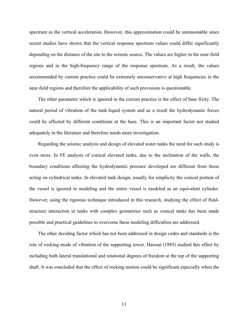
spectrum as the vertical acceleration. However, this approximation could be unreasonable since

recent studies have shown that the vertical response spectrum values could differ significantly

depending on the distance of the site to the seismic source. The values are higher in the near-field

regions and in the high-frequency range of the response spectrum. As a result, the values

recommended by current practice could be extremely unconservative at high frequencies in the

near-field regions and therefore the applicability of such provisions is questionable.

The other parameter which is ignored in the current practice is the effect of base fixity. The

natural period of vibration of the tank-liquid system and as a result the hydrodynamic forces

could be affected by different conditions at the base. This is an important factor not studied

adequately in the literature and therefore needs more investigation.

Regarding the seismic analysis and design of elevated water tanks the need for such study is

even more. In FE analysis of conical elevated tanks, due to the inclination of the walls, the

boundary conditions affecting the hydrodynamic pressure developed are different from those

acting on cylindrical tanks. In elevated tank design, usually for simplicity the conical portion of

the vessel is ignored in modeling and the entire vessel is modeled as an equivalent cylinder.

However, using the rigorous technique introduced in this research, studying the effect of fluid-

structure interaction in tanks with complex geometries such as conical tanks has been made

possible and practical guidelines to overcome these modeling difficulties are addressed.

The other deciding factor which has not been addressed in design codes and standards is the

role of rocking mode of vibration of the supporting tower. Haroun (1985) studied this effect by

including both lateral translational and rotational degrees of freedom at the top of the supporting

shaft. It was concluded that the effect of rocking motion could be significant especially when the

12

coupling between wall flexibility and tank rotation is considered. However, some important

effects were not included in Haroun’s study such as;

1) the liquid was not modeled as a continuous medium and its effect was only

accounted for by an equivalent mechanical model consisting of lumped masses located at

a specific height from the tank floor.

2) liquid sloshing component was neglected in the model proposed for flexible

elevated tanks.

3) emphasis was placed only on the seismic behavior of the supporting structure, no

effort was made to study the dynamic behavior of the vessel.

4) the vessel was assumed to be rigidly connected to the supporting tower that is no

relative rotation could occur between the vessel base and the tip of the tower.

5) vessels in elevated water tanks usually consist of a conical lower section having

inclined side walls. This inclination could have a significant effect on dynamic behavior

of the vessel as well as the supporting shaft. The method proposed in Haroun's study is

not capable of considering this effect.

6) only horizontal excitation can be investigated using Haroun's model.

Considering above-mentioned deficiencies, evaluating the accuracy of current practice by

comparing the code results with those obtained from a rigorous analysis seems necessary.

Throughout this research, effort has been made to address this important objective. The results of

this research provide some useful insights in terms of the dynamic behavior of these types of

structures.

Concerning the dynamic response of ground-supported and elevated water tanks there are

areas in the literature that need to be further investigated. Kianoush and Chen (2006) studied the

13

combined effect of horizontal and vertical ground accelerations in rectangular liquid storage

tanks, however no study has been carried out to consider such effect for cylindrical ones.

The effect of earthquake frequency contents on the dynamic behavior of liquid-filled tanks

need to be investigated by selecting input ground motions having low, intermediate and high

frequency contents and performing a series of rigorous time-history analyses.

In addition, very few studies can be found in the literature regarding the seismic behavior of

liquid-filled conical elevated tanks. The need for proposing a thorough method capable of

considering all deciding parameters and assessing the relative importance of such effects on the

overall seismic response of elevated tanks seems essential. This can be achieved through

performing an extensive parametric analysis encompassing the range of conical elevated tanks

typically found in use today.

Recent investigations show that seismic isolation is an effective alternative for reducing the

vibration amplitude of the structures under seismic waves. However, there are very few studies

in the literature regarding the application of this technique to elevated water tanks. In all of these

studies, the entire system including the isolation system, shaft structure, and contained fluid is

modeled as a discrete three or four-degree-of-freedom model. During this study, effort has been

made to develop a detailed three-dimensional FE model in order to eliminate the inaccuracies

associated with such simplifications in dynamic analysis of isolated elevated tanks. The proposed

model is also capable of accounting for the nonlinear hysteretic behavior of the isolators.

14

1.4 Thesis layout

The outline of this thesis involves nine chapters defined according to the objectives and

scope of the research. The first chapter includes the introduction, the scope, objectives and

significance of the research and the outline of the thesis.

The second chapter presents a summary of the previous research studies carried out on

dynamic response of liquid containing structures, both ground-supported and elevated tanks. An

overview on existing codes, standards, and guides used in design of liquid storage tanks is also

provided in this chapter.

Chapter 3 addresses analytical formulations regarding the calculation of fluid dynamic

response in cylindrical liquid containers. Lamina fluid theory and velocity potential theory

commonly used for obtaining the hydrodynamic pressures and sloshing response of the tanks

under seismic excitations are explained in this chapter.

Chapter 4 deals with the finite element formulation of three-dimensional liquid containing

structures. A discussion on how to consider the fluid-structure coupling effect in finite element

modeling of liquid containing structures is made. In addition, the corresponding equations of

motion of liquid domain accounting for both the impulsive and sloshing components of response

are addressed.

The dynamic behavior of cylindrical ground-supported water tanks is discussed in Chapter

5. Effects of important parameters including sloshing of liquid free surface, tank wall flexibility,

vertical ground acceleration, tank aspect ratio, and base fixity are addressed in this chapter. The

validity of current practice in seismic analysis of liquid-filled cylindrical containers is also

investigated.

15

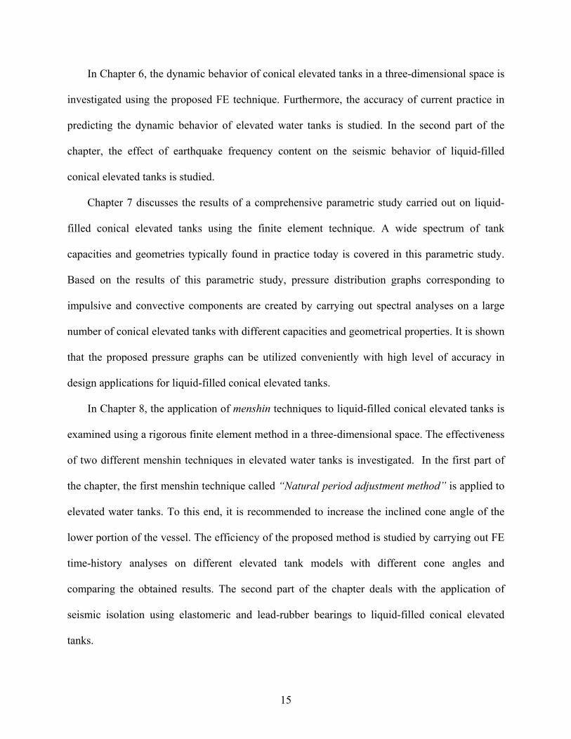
In Chapter 6, the dynamic behavior of conical elevated tanks in a three-dimensional space is

investigated using the proposed FE technique. Furthermore, the accuracy of current practice in

predicting the dynamic behavior of elevated water tanks is studied. In the second part of the

chapter, the effect of earthquake frequency content on the seismic behavior of liquid-filled

conical elevated tanks is studied.

Chapter 7 discusses the results of a comprehensive parametric study carried out on liquid-

filled conical elevated tanks using the finite element technique. A wide spectrum of tank

capacities and geometries typically found in practice today is covered in this parametric study.

Based on the results of this parametric study, pressure distribution graphs corresponding to

impulsive and convective components are created by carrying out spectral analyses on a large

number of conical elevated tanks with different capacities and geometrical properties. It is shown

that the proposed pressure graphs can be utilized conveniently with high level of accuracy in

design applications for liquid-filled conical elevated tanks.

In Chapter 8, the application of menshin techniques to liquid-filled conical elevated tanks is

examined using a rigorous finite element method in a three-dimensional space. The effectiveness

of two different menshin techniques in elevated water tanks is investigated. In the first part of

the chapter, the first menshin technique called “Natural period adjustment method” is applied to

elevated water tanks. To this end, it is recommended to increase the inclined cone angle of the

lower portion of the vessel. The efficiency of the proposed method is studied by carrying out FE

time-history analyses on different elevated tank models with different cone angles and

comparing the obtained results. The second part of the chapter deals with the application of

seismic isolation using elastomeric and lead-rubber bearings to liquid-filled conical elevated

tanks.

16

In Chapter 9, conclusions and some suggestions for future work are presented. The thesis

ends with a list of references and three appendices. In the first appendix, details of the lamina

fluid theory discussed in Chapter 3 are presented. The second appendix provides the input text

command files for the tank’s parametric model and the post-processors used in Chapter 7. The

pressure distribution graphs obtained through the parametric study explained in Chapter 7 are

given in the third appendix.

17

CHAPTER 2

LITERATURE REVIEW

2.1 Introduction

In this chapter an extensive literature review on dynamic response of liquid containing

structures is presented. In Section 2.2 seismic performance of liquid storage tanks and associated

damage types suffered during actual seismic events is discussed. Section 2.3 reviews and

summarizes the available literature on seismic response of liquid storage tanks. Both ground-

supported and elevated tanks are addressed. The significant contributions made by previous

researchers are also explained. An overview on existing codes, standards, and guides used in

design of liquid storage tanks along with a literature review on application of seismic isolation to

liquid storage tanks are provided in Section 2.4.

2.2 Earthquake damage to liquid storage tanks

There are frequent reports regarding the damage to liquid storage tanks due to previous

earthquakes in the literature. For instance, there were heavy damages to both concrete and steel

storage tanks during the strong seismic events such as 1933 Long Beach, 1952 Kern County,

1964 Alaska, 1964 Niigata, 1966 Parkfield, 1971 San Fernando, 1978 Miyagi prefecture, 1979

Imperial County, 1983 Coalinga, 1994 Northridge, and 1999 Kocaeli earthquakes (Rinne (1967),

Shibata (1974), Kono (1980), Manos and Clough (1985), and Sezen and Whittaker (2006)).

Severe damage levels were also observed in elevated water tanks during the 1960 Chilean as

well as the 1997 Jabalpur (Rai et al. (1997)) and 2001 Bhuj (Rai (2002) and Dutta et al. (2009))

earthquakes in India. During the Bhuj earthquake many elevated tanks suffered severe damages

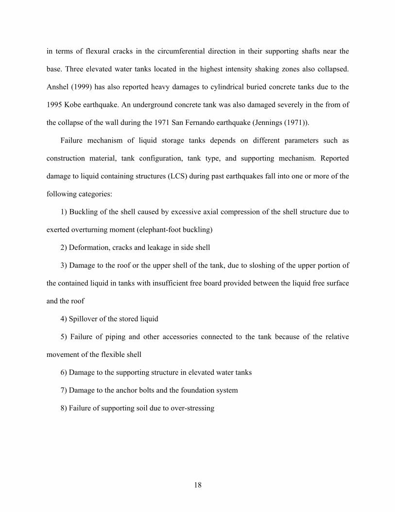
18

in terms of flexural cracks in the circumferential direction in their supporting shafts near the

base. Three elevated water tanks located in the highest intensity shaking zones also collapsed.

Anshel (1999) has also reported heavy damages to cylindrical buried concrete tanks due to the

1995 Kobe earthquake. An underground concrete tank was also damaged severely in the from of

the collapse of the wall during the 1971 San Fernando earthquake (Jennings (1971)).

Failure mechanism of liquid storage tanks depends on different parameters such as

construction material, tank configuration, tank type, and supporting mechanism. Reported

damage to liquid containing structures (LCS) during past earthquakes fall into one or more of the

following categories:

1) Buckling of the shell caused by excessive axial compression of the shell structure due to

exerted overturning moment (elephant-foot buckling)

2) Deformation, cracks and leakage in side shell

3) Damage to the roof or the upper shell of the tank, due to sloshing of the upper portion of

the contained liquid in tanks with insufficient free board provided between the liquid free surface

and the roof

4) Spillover of the stored liquid

5) Failure of piping and other accessories connected to the tank because of the relative

movement of the flexible shell

6) Damage to the supporting structure in elevated water tanks

7) Damage to the anchor bolts and the foundation system

8) Failure of supporting soil due to over-stressing

19

In the 1964 Niigata earthquake, several damage modes including damage modes 3 and 4 due

to excessive sloshing, mode 8 due to liquefaction of the supporting soil as well as damage modes

7 and 5 became prominent.

In the 1964 Alaska and 1971 San Fernando earthquakes, the lower part of the side shell

bulged all along the perimeter as a result of mode 1 (elephant-foot buckling). This buckling type

damage generally happens due to the excessive overturning moment generated during the

seismic event.

In cases where the tank contains hazardous materials, liquid spillover (damage mode 4) and

fire subsequent to a major earthquake may result in even more severe damage than the

earthquake itself. The extensive uncontrolled fire eruption during the Niigata earthquake at

Showa Petroleum blazed for about 15 days, resulting in main destruction of the plant and

residential apartments (Niigata Nippo Co. (1964)). The Niigata and Alaska earthquakes of 1964

resulted in considerable loss in the petroleum storage tanks. This significant loss attracted many

practicing engineers and researchers to further investigate the seismic behavior of liquid storage

tanks especially when the stored liquid is a hazardous material such as petroleum.

As an example of damage mode 4, one can mention oil spillover into the harbor that

happened in the Sendai Refinery of Tohoku Petroleum Company during the 1978 Miyagi

earthquake (Hazardous Material Technology Standards Committee: Fire Defense Agency

(1979)).

During the Northridge earthquake main lifeline facilities of the Los Angeles area

experienced severe damage. Five steel tanks were also damaged in the San Fernando Valley area.

Buckling was the prominent form of damage in all of the damaged tanks. Several other tanks

also suffered roof collapse due to the excessive sloshing of the stored liquid (Lund (1996)).

20

It is important to note that the damage mode in concrete tanks is different from that of steel

tanks. Elephant-foot buckling, anchorage system failure, and sloshing damage to the roof and

upper shell of the tank are the most common damages in steel tanks (see Figure 2.1).

In tanks found in practice, full base anchorage is not always a possible or economical

alternative. Therefore, many tanks are either unanchored or partially anchored at their base. If

the tank is not rigidly anchored to the ground, the generated overturning moment due to

earthquake may be large enough to result in lift-off of the tank base. As the tank base falls back

down after lift-off, high compressive stresses are generated in the wall near the base leading to

elephant-foot wall buckling. This mode of damage is more common in steel tanks since they are

generally more flexible than concrete tanks.

Some studies show that base lift-off in tanks having flexible soil foundations does not cause

high axial compressive stresses in the tank wall. As a result, unanchored tanks flexibly supported

at their base are less susceptible to elephant-foot buckling mode, but are more susceptible to

uneven settlement of the foundation (Malhotra (1995) and Malhotra (1997A)).

On the other hand, damage mode 2 is the most common type of damage in concrete tanks.

Stresses caused by large hydrodynamic pressures together with the additional stresses resulted

from the large inertial mass of concrete could cause cracking, leakage and ultimately failure of

the tank. That is why the design criteria for concrete tanks are based on crack control.

It is worth noting that elevated water tanks are very susceptible to seismic excitations

because of the concentrated large mass located at top of the shaft structure. As a result, strong

lateral seismic motions may result in large tensile stresses on one side of the concrete shaft

section which may eventually lead to severe cracking or even collapse of the concrete pedestal.

21

As mentioned before, many elevated tanks collapsed during the 1960 Chilean, 1997 Jabalpur and

2001 Bhuj earthquakes since insufficient reinforcement was provided in the shaft section.

(a)

(b)

(c)

Figure 2.1 Common damage modes: (a) Elephant-foot buckling, (b) Inelastic stretching of

an anchor bolt at the tank base (c) Sloshing damage to the upper shell of the tank

(adapted from Malhotra et al. (2000) and Malhotra (2000))

22

The significance of preventing such damages has led to a great deal of research to be carried

out on dynamic behavior of such structures. These research studies could result in a better

comprehension of the complicated behavior of liquid containing structures under seismic

excitations.

2.3 Previous research

2.3.1 Response of ground-supported tanks

A comprehensive research work on dynamic behavior of liquid-filled tanks has been carried

out both theoretically and experimentally. Initial studies involved analytical investigation of

dynamic response of liquid containing structures having rigid wall and supported on rigid

foundations. Extensive study on the dynamic behavior of liquid containing structures started in

the late 1940’s. Jacobsen (1949) and Jacobsen and Ayre (1951) studied the dynamic response of

cylindrical tanks subjected to horizontal ground motions. They estimated the effective

hydrodynamic masses and mass moments for the accelerated contained liquid.

In the early 1960s, Housner (1963) proposed a useful idealization for obtaining liquid

response of rigid rectangular and cylindrical water tanks fully anchored to the rigid foundation

and subjected to horizontal ground motion. Liquid was assumed to be incompressible and

inviscid. This method is probably one of the most well-known procedures available in the

literature. However, attention should be drawn to the effect of tank wall flexibility which is not

considered in this simplified technique. Housner separated the tank hydrodynamic response into

"impulsive" motion, in which the liquid is assumed to be rigidly attached to the tank and moves

in unison with the tank shell, and "convective" motion, which is characterized by long-period

oscillations and involves vertical displacement of the fluid free surface. Under seismic motions,

23

impulsive water undergoes the same acceleration as the ground. This component is believed to

have a significant contribution to the base shear and base moment. In this study, Housner

developed simple equations to approximate the hydrodynamic pressures in the tanks using

lumped mass approach.

Many current standards and guides such as ACI 350.3-06 and ACI 371R-08 have adapted

Housner's method with some modifications which were the results of subsequent studies by other

researchers for seismic design of liquid storage tanks. As mentioned before Housner's method is

not capable of accounting for the effect of tank wall flexibility. Therefore, as an approximate

method ACI 350.3-06 accounts for wall flexibility by determining the oscillating water mass

components from the rigid tank solution and only using the amplified pseudoacceleration

corresponding to the fundamental natural frequency of the system instead of the ground

acceleration. This approximation may be unduly inaccurate for values of H/R (liquid depth/tank

radius) greater than 1 (Veletsos (1984)).

Edwards (1969) for the first time suggested a finite element method to be employed for

estimating the seismic response of deformable liquid storage tanks. A cylindrical liquid storage

tank with the height to diameter ratio of less than one was analyzed using the finite element

technique. The proposed FEM was capable of accounting for the coupled interaction between the

stored liquid and the elastic tank shell.

Using Housner’s model, Epstein (1976) produced design curves for calculating the

overturning moment due to hydrodynamic pressures in both rectangular and cylindrical storage

tanks.

Veletsos (1974) and Yang (1976) showed that the flexibility of the tank shell could have a

significant effect on dynamic forces induced by horizontal ground motion in liquid-filled

24

cylindrical containers. It was concluded that the flexibility of the walls of such tanks has a

substantial effect on the impulsive component of the response. Veletsos and Yang (1977)

modified this method by using Flugge's shell theory (Flugge, 1960) in combination with the

Rayleigh-Ritz procedure to calculate the natural frequencies of the liquid-shell system. Both

shell analysis and the simpler beam-type analysis were carried out.

The dynamic behavior of horizontally accelerated liquid storage tanks containing inviscid

liquid was further investigated by Hunt and Priestley (1978). Both rectangular and cylindrical

configurations were examined. The results of the study led to derivation of mathematical

equations regarding the contained fluid motion under dynamic excitations. The displacement of

liquid free-surface was measured experimentally for a cylindrical water tank tested on a shaking

table and subjected to both sinusoidal and seismic excitations. The predicted theoretical results

were in close agreement with those obtained through experiment.

Clough and Clough (1977) and Clough et al. (1979) for the first time performed a series of

experimental tests on large-scale thin-walled liquid storage tanks. The obtained hydrodynamic

pressures were much larger than those proposed by Housner’s analytical method. The difference

in pressures was believed to be due to the tank wall flexibility effect. Several other numerical

and analytical studies taking into account the interaction between flexible shell and the

containing liquid were conducted among which significant contributions were made by Haroun

(1980) and Barton and Parker (1987).

Haroun and Housner (1981A) studied the behavior of deformable liquid storage tanks using

modal superposition analysis. In this study, the tank shell was modeled by finite elements and the

fluid domain was treated mathematically using boundary solution technique.

25

Haroun and Housner (1981B) developed a mechanical model capable of including the effect

of wall deformability. The proposed three-degree-of-freedom (DOF) mechanical model involved

three equivalent lumped masses corresponding to the convective component contributed by the

sloshing of the liquid, the impulsive component which varies in unison with the horizontal

ground acceleration, and the short period component contributed by the deformable wall

vibrations. The latter component is only present in flexible liquid containers. In a tank with rigid

wall boundary condition, only the first two components need to be considered. The study also

showed that the tank wall deformability may result in the hydrodynamic pressures several times

larger than those experienced in rigid wall tanks. Based on this study, design charts for

estimating the equivalent lumped masses of the proposed mechanical model were derived. It was

assumed that the liquid contained in the tank was incompressible and had irrotational flow.

Balendra et al. (1982) presented a finite element analysis of an annular cylindrical tank with

an axisymmetric elastic dome, using a FE code. The fluid inside the tank was considered as

inviscid and incompressible. However, sloshing of the fluid was neglected.

Minowa (1980 and 1984) further studied the tank wall flexibility effect and the

corresponding hydrodynamic pressure exerted on the tank shell. He also performed experimental

studies on the dynamic behavior of rectangular liquid-filled tanks.

Haroun (1983) also performed a series of experimental investigations including forced and

ambient vibration tests on flexible ground-supported cylindrical tanks. In order to determine the

mode shapes of vibrations and corresponding natural frequencies, three full scale water storage

tanks were tested. This study led to a better understanding of dynamic behavior of liquid storage

tanks.

26

Haroun (1984) evaluated the dynamic response of rectangular concrete liquid storage tanks

using the classical potential flow approach assuming a rigid wall boundary condition. The fluid

was assumed to be homogeneous, incompressible and inviscid. The tank was assumed to be

subjected to the simultaneous action of horizontal and vertical components of earthquake.

Bending moments developed in the walls of rectangular liquid-filled tanks due to seismic

excitation at their base were calculated. As a result of this study, theoretical equations to evaluate

the internal moments in the tank wall were derived and numerical values of moment coefficients

to be used in seismic design of rectangular tanks were tabulated.

Veletsos and Kumar (1984) developed a simplified approach for estimating the effect of

vertical ground motion on cylindrical liquid storage tanks.

Haroun and Tayel (1985) employed the finite element technique for investigating the

dynamic behavior of cylindrical liquid storage tanks having elastic wall and subjected to vertical

seismic excitations. The proposed method was based on the superposition analysis technique

using the axisymmetrical free vibration modes of the tank-liquid system. The axial and radial

components of the wall displacement together with the resulting stresses were calculated. In

obtaining the dynamic response of the tanks, effect of liquid sloshing was ignored.

Veletsos and Tang (1990) studied the dynamic behavior of liquid containing tanks resting on

flexible foundations through rigid base mats. The results of the study indicated that the

translational and rocking vibrations of the tank base resulted in extended impulsive period and

also larger effective damping. They had previously concluded that soil-structure interaction

reduces the hydrodynamic effects in tanks subjected to vertical excitations (Veletsos and Tang

(1986)).

27

Park et al. (1992) used a coupled boundary element-finite element method (BEM-FEM) to

study the dynamic behavior of concrete rectangular tanks. The dynamic response of the tanks

was obtained using the time-history analysis method. Both impulsive and convective components

were included.

Coupled free vibration dynamics of cylindrical liquid storage tanks was studied by Gupta

(1995). The vibration study of the container was made possible using Flugge’s exact equations of

motion. The hydrodynamic pressure associated with the contained liquid was obtained using the

velocity potential approach. The obtained results compared well with those calculated by Haroun

and Housner method.

Kim et al. (1996) used Rayleigh-Ritz method to study the dynamic response of a flexible

rectangular liquid storage tank. In this study, the effect of sloshing component of the contained

liquid was neglected.

The dynamic response characteristics of rectangular fluid containers was further studied by

Dogangun et al. (1997 and 2004). He used analytical methods as well as finite element method

using the modified structural analysis program SAPIV to evaluate the dynamic response. The

fluid domain was modeled by displacement-based fluid elements. Effect of tank wall flexibility

on dynamic behavior of tanks was also investigated. The proposed model was capable of

including the effects of fluid compressibility and free-surface sloshing motion. The obtained FE

results were compared with those obtained through boundary-finite element method (BEM-

FEM) and requirements of Eurocode-8.

Koh et al. (1998) proposed a coupled BEM-FEM technique including free-surface sloshing

vibration, to investigate the dynamic behavior of three dimensional rectangular water storage

tanks under horizontal ground motions. In their study, finite element method was employed to

28

model the solid wall while the indirect boundary element method was used to model the fluid

domain.

In a study by Chen and Kianoush (2005) a new procedure called sequential method for

estimating the hydrodynamic pressures in rectangular tanks was introduced. In this method,

fluid and structure domains are coupled through applying the results from the first analysis as

loads or boundary conditions for the second analysis. The study was performed in a two-

dimensional space and the effect of tank wall flexibility was also included. However, the effect

of fluid sloshing was not taken into account.

Virella (2006) investigated the natural periods, mode shapes, and dynamic response to

horizontal ground excitations of cylindrical tanks partially filled with a liquid. The finite element

package ABAQUS was used to perform the computations. The contained fluid was modeled

using two different techniques: the added mass formulation and acoustic fluid elements based on

linear wave theory. The considered tanks had the height to diameter ratios from 0.40 to 0.95. No

sloshing waves were considered in the study. It was concluded that the response of a tank-liquid

system under horizontal excitation can be precisely estimated by considering just the

fundamental mode. Furthermore, it was verified that the tanks with height to diameter ratios

larger than 0.63 have the fundamental modes similar to the first mode of a cantilever beam. For

the shortest tank considered in the study (H/D = 0.4), the fundamental mode was a bending

mode.

The dynamic behavior of rectangular containers under vertical seismic excitations was also

investigated in a later study by Kianoush and Chen (2006) in a two-dimensional space. It was

concluded that the vertical ground excitation could cause significant seismic response in

rectangular concrete tanks and therefore such effect should be considered in design.

29

A new approach for seismic analysis of rectangular liquid storage tanks in time domain

taking into account the effects of both impulsive and convective components was introduced by

Kianoush et al. (2006). The method was able to solve the coupled liquid-filled tank problem in

three-dimensional space.

Ghaemmaghami et al. (2010) investigated the seismic behavior of both concrete rectangular

and cylindrical liquid storage tanks in three-dimensional space. The containers were assumed to

be fixed to the rigid ground. Both impulsive and sloshing components of response were

considered. The tank models were analyzed in time domain under the horizontal and vertical

components of a real earthquake record. Fluid-structure interaction effects were taken into

account incorporating wall flexibility. The study indicated that the effect of vertical excitation on

the seismic response of the liquid tanks could be significant when considered individually,

however it was of less significance when the horizontal and vertical earthquake components

were applied together. This was valid for both rectangular and cylindrical tanks.

As opposed to ground-supported liquid storage tanks, limited number of literature is

available regarding the dynamic response characteristics of elevated water tanks. Several

attempts have been made over the past few decades to investigate the fluid-structure interaction

effects in elevated water tanks.

2.3.2 Response of elevated tanks

The well-known Housner method enabled practicing engineers to carry out the seismic

response analysis of elevated tanks using a two-mass idealization (Housner 1963). This

simplified model allowed for the motion of water relative to the tank as well as the motion of the

tank relative to the ground. Further application of such simple model in seismic analysis of

30

elevated tanks was reported by Sonobe (1969). In this study, both free vibration and stationary

vibration tests were performed on two scale models of elevated water tanks. The first model was

a cylindrical tank model supported by a frame which had several levels of rigidity. The ratio of

the model to the prototype was 1/10 – 1/20. The second model was a spherical tank of the same

size. Furthermore, a forced vibration test under the input of pseudo El-Centro NS 1940 record

was carried out on the cylindrical elevated tank model. From the test, the dynamic response of

the tank including maximum displacement and acceleration of the frame and maximum sloshing

height of the stored water was measured. Experimental results were in good agreement with

those obtained from the analytical solution using a simplified two-DOF system. In creating this

equivalent model, the weight of the frame plus dead water was assumed to be rigidly fastened to

the tank, while the weight of free water was assumed to be attached to the tank by means of

springs.

Some researchers such as Chandrasekaran and Krishna (1965) and Tamiah and Gupta

(1966) proposed that a satisfactory estimation of dynamic response of elevated water tanks may

be obtained using a single-DOF model.

Shepherd (1972) also used a two-mass idealization model to represent the dynamic behavior

of elevated water tanks. The validity of the model was verified by comparing the analytical

values with those of a simple dynamic test conducted on a prestressed concrete elevated water

tank. The examined tank was a prestressed concrete tubular tower supporting a cylindrical

reinforced concrete tank. The equivalent water masses, the moment arms, and the effective

spring stiffness were calculated using Housner’s formulation. The predicted natural frequencies

of the two modes of vibration obtained through analytical solution were compared with those

measured through a simple pull-back test. The sloshing frequency of the water inside the tank

31

was determined by hand shaking tests. The percentage equivalent viscous critical damping was

determined from the decay of the free vibration test results as 1.3%. The results of the study

indicated that the use of a two mass equivalent model will provide satisfactory estimations of the

natural frequencies of the elevated water tanks.

Ifrim and Bratu (1969) and Garcia (1969) also used a two-DOF representation to investigate

the seismic response of elevated tanks.

Haroun and Ellaithy (1985) presented an equivalent mechanical model for evaluating the

dynamic response of elevated water tanks. A cross braced frame as well as a concrete pedestal

tower were analyzed. The effect of tank wall flexibility and both rocking and translational

motions of vessel were included in the study. Analyses indicated that the rocking component of

vessel could have a significant effect on maximum shear and moment exerted at the top of the

tower. However, in their study the vessel was assumed to be rigidly connected to the supporting

tower that is no relative rotation could occur between the vessel base and the tip of the tower.

Following the collapse of a conical tank in Belgium during the 1970s, an experimental

research work was carried out on the stability of conical tanks under hydrostatic loading by

Vandepitte et al. (1982). A similar problem was further addressed by El Damatty et al. (1997A)

using an extensive numerical study. In this study, a finite element model capable of including

both geometric and material non-linearities for stability analysis of liquid-filled conical tanks

under hydrostatic loading was proposed. The effect of geometric imperfections on the stability of

such structures was examined. The effect of such imperfections was modeled by introducing

initial strains into the finite element model of the tank before applying the loads.

Joshi (2000) presented an equivalent mechanical model for seismic analysis of rigid intze

type tanks under horizontal acceleration. Model parameters were evaluated for a wide spectrum

32

of tank shapes and compared with those of the equivalent cylindrical tanks. Fluid pressure was

calculated using linearized potential flow theory. The fluid was assumed inviscid and

incompressible and the sloshing height was assumed to be small. Furthermore, in developing the

mechanical model only first sloshing mode was taken into account. It was concluded that the

associated errors due to the use of equivalent cylindrical tank model instead of the original intze

tanks were negligible. As a result, for design applications, the intze tank models may be replaced

by the equivalent cylindrical models without loss of accuracy.

Seismic behavior of elevated conical steel tanks was studied by El Damatty et al. (1997B;

1997C). In the study, a numerical model was developed in which the tank wall was modeled by

shell elements and the fluid effect was considered using the coupled boundary-shell element

technique. Only the impulsive component of the hydrodynamic pressure was considered. Several

tank models classified as tall or broad according to their aspect ratio (the ratio of the tank radius

to its height) were taken into consideration. The supporting structure was accounted for by

adding linear springs to the vessel base and the vessel was also prevented from rocking. The

effects of both material and geometric nonlinearities were included in the model. Both free

vibration and non-linear time history analyses were carried out. It was concluded that elevated

conical tanks, especially the tall tanks, are very sensitive to seismic excitations and their design

must be based on large static load factors in order to be safe during strong seismic events. It was

also indicated that the vertical ground motion contributes significantly to the dynamic instability

of conical elevated tanks and as a result its effect must be included properly in seismic analysis

of such structures.

Later, El Damatty et al. (2000) proposed an analytical model for estimating the free surface

sloshing response of conical tanks under dynamic motions. The model was applicable to both

33

purely conical and combined conical-cylindrical vessels. It was assumed that the sloshing

response could be estimated while considering the rigid wall boundary condition. The shell

vibration was determined assuming zero hydrodynamic pressure at the liquid free-surface. The

validity of this analytical model was verified in a later experimental study carried out by

Sweedan and El Damatty (2002) on a small-scale purely conical tank.

The dynamic characteristics of liquid-filled combined vessels in which vessels consisted of a

conical steel section with superimposed top cylindrical shell were identified experimentally in

later studies by El Damatty (2005). This study was the first experimental study carried out on a

small-scale liquid-filled conical vessel. The fundamental frequencies as well as the frequencies

of cos(θ)-modes of vibration were determined using shake table test. The experimental values

were compared with those obtained from the analytical and numerical methods and in general an

excellent agreement was observed. It was found that the cos(θ)-modes which lead to base shear

and overturning moment in tanks subjected to seismic motions, show themselves as higher

modes of vibration.

Sweedan and El Damatty (2005) investigated the dynamic response of purely conical tanks

under vertical acceleration. It was shown that vertical excitation of such tanks could cause

significant increase in the compressive meridional stresses generated in the tank walls.

To further simplify the seismic analysis of elevated tanks, Sweedan (2009) proposed an

equivalent mechanical model to duplicate forces induced in combined elevated tanks subjected to

vertical ground acceleration. The proposed model was able to consider the flexibility of the tank

wall. The stored liquid was modeled as flexible and rigid components. The flexible component

was associated with the vibration of the tank walls, while the rigid component vibrated in

synchronism with the base excitation. Parametric analyses were performed to evaluate the

34

natural frequencies of the axisymmetrical modes of vibration. The contribution of the stored

liquid mass to the impulsive response was also determined by performing modal analyses.

Moslemi et al. (2011) evaluated the performance of conical elevated tanks under seismic

motions. The FE technique was employed to estimate the seismic response. Both time history

and free vibration analyses were carried out. The effects of liquid sloshing and tank wall

flexibility were considered in the proposed FEM. The obtained results were also compared with

those recommended by current practice (ACI 350.3-06 in conjunction with ASCE 7-05). In this

study, the difficulties associated with modeling of the tanks having complex geometries such as

conical shaped vessels were addressed. The accuracy of the method was verified by comparing

the obtained results with experimental and numerical values available in the literature. Modal FE

analyses resulted in natural frequencies and effective water mass ratios very close to those

obtained from Housner's formulations. The results of the study also showed that the current

practice could predict the dynamic response of elevated water tanks with reasonable accuracy.

Further details on this study will be presented in this thesis.

2.4 Other related studies

2.4.1 Application of seismic isolation to liquid storage tanks

The application of base isolation technique to buildings and bridges has been extensively

developed in the past. However, a few studies regarding such application to liquid storage tanks

can be found in literature. Base isolators both deflect and absorb the seismic input energy

transmitted to the structure. Seismic isolation is normally suggested for the rehabilitation of

structures expecting to have unsatisfactory performance under seismic events. There are

examples of such application to liquid storage tanks in practice. For instance, in Seattle several

35

elevated water tanks were proposed to be rehabilitated using this technique (Bleiman and Kim

(1993)). The tanks under consideration were very large capacity storage tanks. After performing

detailed analyses on seismic isolation and other conventional rehabilitation alternatives, the

project engineers came to the conclusion that seismic isolation technique was the most effective

and cost-efficient rehabilitation option.

As a result, seismic isolation may be considered as an easy and economical technique for

such structures, especially in moderate to high seismic intensity zones in which the design of the

structure is governed by seismic loads.

Chalhoub and Kelly (1990) carried out shake table tests on fixed base as well as base

isolated ground-supported tanks. A substantial reduction in total hydrodynamic pressure and base

reaction values was reported. However, a slight increase in the free-surface sloshing height of the

isolated tank relative to the fixed base tank was observed.

Bo and Jia-xiang (1994) modeled an isolated ground-supported tank using FE method. Only

a single earthquake record was considered. The results showed reduction in hydrodynamic

pressures, shell amplitudes, and liquid sloshing height as a result of isolation.

Kim and Lee (1995) conducted an experimental study on isolated liquid containers. They

performed a series of pseudodynamic tests incorporating a substructuring technique on the

isolated liquid storage tanks subjected to uni-directional acceleration. Two types of tanks namely

tall and broad were tested to predict the hydrodynamic forces. In the testing algorithm, the base

isolators were tested as the tested part, while the tank was simulated in a computer with a proper

modeling technique as the computed part. The liquid storage tank was modeled as a discrete

mechanical model. The effect of stored liquid was accounted for using three equivalent lumped

masses. The tanks were isolated by laminated rubber bearings. Free vibration tests as well as

36

seismic tests using real earthquake records were carried out. The seismic isolation was found to

be quite effective in reducing the dynamic response.

The seismic performance of ground-supported tanks having various isolation and energy

dissipation mechanisms was further investigated by Malhotra (1997B, 1997C, and 1998).

Several rehabilitation solutions including vertical isolation, lateral isolation, and passive

energy dissipation devices as hold-down anchors were investigated. In all cases, significant

improvement in the seismic behavior of the tanks under consideration was reported. However, a

slight increase in the free surface sloshing height in the laterally isolated tank was observed. In

these studies, a new method for seismic isolation of ground-supported cylindrical tanks was

proposed. In this method, the tank wall was disconnected from the base plate and was supported

on a ring of isolation bearings. The base plate was resting directly on the ground. A flexible

membrane was used between the wall and the base plate in order to prevent the liquid leakage

from the tank and also to allow the free movement of the wall. It was shown that this isolation

scheme could reduce substantially the dynamic base shears, overturning moments, and axial

compressive stresses in the wall of the tank. However, since the weight applied on the bearings

was small compared to the total weight of the stored fluid, a net tensile force was observed in the

bearings of the tall tanks subjected to strong seismic excitations.

Shenton III and Hampton (1999) studied the seismic response of isolated elevated water

tanks using a discrete three-DOF model. The natural frequencies and mode shapes of the isolated

structure were determined and response spectral analyses were carried out. Only a linear elastic

isolation system was considered. Furthermore, the tank walls were assumed to be rigid and the

effect of rocking of the tower on dynamic response was ignored. Isolation bearings were

assumed to be effectively rigid in the vertical direction. Results of the isolated tank models were

37

compared with those of the corresponding non-isolated tank models and it was concluded that

the base isolation was effective in reducing the seismic response of the liquid-filled elevated

tanks. It was also shown that isolation was most effective for the smallest capacity tank.

Shirmali and Jangid (2003) investigated the seismic behavior of isolated elevated tanks

under real earthquake excitations using a four-DOF model. The isolation system considered was

lead-rubber bearings. The fluid domain was modeled as lumped masses. Isolators were assumed

to be effectively rigid in the vertical direction. As a result, the effects of uplift and rocking were

not considered. It was observed that the seismic response of the isolated tanks was reduced

significantly. In addition, a simplified decoupled analysis was proposed in which the motion of

tower structure was assumed to be rigid under seismic excitation. This assumption led to a two-

DOF model and two single-DOF models. It was concluded that this simplified method could

accurately estimate the peak seismic response of the isolated elevated tanks with less

computational efforts.

Later, Jadhav and Jangid (2004) investigated the dynamic behavior of liquid storage tanks

isolated by elastomeric bearings and sliding mechanism under real earthquake records. The fluid

domain was modeled as sloshing, impulsive, and rigid lumped masses. The same model was

employed to study the seismic behavior of liquid storage tanks subjected to near-fault ground

excitations (Jadhav and Jangid (2006)).

Shekari et al. (2009) further investigated the seismic behavior of isolated cylindrical liquid

storage tanks under horizontal ground motions in a three-dimensional space. The structure was

modeled by finite shell elements while the fluid domain was simulated using the internal

boundary elements. The base isolation system was modeled by bilinear hysteretic elements. It

was indicated that the dynamic response of isolated tanks could be dramatically reduced

38

compared to the fixed base tanks. However, it was observed that the liquid free surface

displacement was increased due to base isolation. It was also concluded that the base-isolation

system was more effective when the stiffness of base isolators was smaller. However, the

isolators should be stiff enough to assure the tank stability.

2.4.2 Codes and standards

In this section a brief review on various codes and standards available for seismic design of

liquid containing structures is presented. The main focus is on the codes and standards used in

North America. International Building Code, IBC (2011) is one of the most comprehensive and

preferred codes currently used in the United States. In the last revision of this code, the ASCE 7-

10 (2010) standard is referred to for seismic design of common liquid storage tanks. In ASCE 7-

10, the input ground motion is defined as a response spectrum corresponding to the Maximum

Considered Earthquake (MCE) which represents an earthquake with a 2% probability of

exceedance in a 50-year period (equivalent to a recurrence interval of approximately 2500 years).

Currently, there are no direct guidelines for structural design of environmental structures in

Canadian design standards. However, useful guidelines may be found in a variety of other codes

and standards such as ACI 350.3-06 (2006), New Zealand Standard NZS 3106 (2010), European

Eurocode-8 (2006), and British Standard BS 8007 (1987), among which ACI 350.3-06 is the

most comprehensive and widely adopted one.

ACI 350.3-06 standard reported by the American Concrete Institute, Committee 350 is

presently used as an obligatory document for seismic design of reinforced concrete liquid storage

tanks in North America. Supplementary guidelines regarding the analysis and design of elevated

concrete and composite steel-concrete water storage tanks may be found in ACI 371R-08 (2008).

39

The Committee 350 was formed by the American Concrete Institute (ACI) in 1964 as a

technical board responsible for providing guidelines for the design of environmental engineering

structures. In 2001, ACI published the first standard for design of environmental engineering

concrete structures in North America (ACI 350-01 and ACI 350.3-350.3R-01). In that standard,

two different methods of design (working stress method and modified ultimate strength method)

were proposed. The design methods were calibrated in such a way to provide comparable but not

necessarily identical designs.

Current revision of the Code (ACI 350.3-06) is based on the ultimate strength design

method. In this standard, an equivalent mechanical model based on the Housner’s method

(Housner (1963)) has been incorporated by which the resultant seismic forces acting on the walls

of rigid containers can be estimated.

Two different standards intended for the design of prestressed concrete liquid storage tanks

were published by the American Water Work Association (AWWA); AWWA D110 (1995), and

AWWA D115 (1995). The guidelines regarding the design of welded steel liquid storage

containers were provided in AWWA D100 (2005).

The American Petroleum Institute (API) published two standards; API 650 (1998), and API

620 (1998) for the design of tanks used in the petroleum industry.

American Society of Civil Engineers (ASCE) provided two publications including useful

guidelines regarding the seismic design of storage tanks used in the nuclear industry; ASCE 4-98

(1998), and ASCE 58 (1980). Tanks used in the nuclear industry should meet more stringent

design requirements compared to those used in other industries because of the potential hazard of

radioactive materials to public safety.

40

Most of the standards including ACI 350.3-06, AWWA D100, AWWA D110, and API 650

have employed the Housner’s mechanical model (Housner (1963)) with some modifications for

determining the seismic forces associated with the accelerated contained liquid. In NZS 3106

(2010), the mechanical model proposed by Veletsos and Yang (1977) is used for seismic analysis

of rigid tanks while the model developed by Haroun and Housner (1981B) is used for

deformable liquid storage tanks.

In Eurocode-8 (2006) the dynamic analysis of rigid circular tanks is performed using

Veletsos and Yang’s model (1977). Models developed by Veletsos (1984) and Haroun and

Housner (1981B) together with the approach proposed by Malhotra et al. (2000) are used for

dynamic analysis of flexible circular tanks. Housner’s method (1963) is recommended for

seismic evaluation of rigid rectangular tanks, while no practical approach is assigned for flexible

rectangular containers.

In seismic design, the seismic response values corresponding to the impulsive and

convective parts are combined using an appropriate combination method. All codes and

standards except the Eurocode-8, recommend SRSS (Square Root of Sum of Squares) rule to be

used for combining the impulsive and convective seismic effects. Eurocode-8 suggests absolute

summation combination rule.

Different standards specify different damping values to be considered for impulsive

component. However, all codes and standards agree on the damping ratio of 0.5% to be used for

convective component. ACI 350.3-06, ASCE 7-05, AWWA D100, AWWA D110, AWWA

D115, and API 650 recommend a damping ratio of 5% for impulsive component for all tank

types. In Eurocode-8, a damping ratio of 5% is proposed for the impulsive component of

concrete tanks while 2% damping is specified for steel tanks. As a result of different damping

41

ratios associated with impulsive and convective liquid components, different response spectra

corresponding to these components are provided in LCS design codes and standards.

In NZS 3106 (2010), the appropriate damping ratio for the impulsive component is

determined based on the tank geometry, tank aspect ratio, tank material, and shear wave velocity

in foundation soil.

42

CHAPTER 3

THEORETICAL ANALYSIS

3.1 Introduction

Fluid dynamic response using analytical formulations is addressed in this chapter. Two

important theories namely lamina fluid theory and velocity potential theory capable of predicting

the hydrodynamic pressure applied by the fluid on the tank wall and maximum sloshing heights

due to seismic motions are described. For design purposes, the resulting hydrodynamic forces

can be obtained by integrating the hydrodynamic pressures over the wetted area. All derived

formulations are based on the basic theory of linear sloshing.

This chapter deals with the fluid response to pure lateral excitations for typical upright

cylindrical containers. Also, the development of equivalent models as approximate mechanical

systems used in dynamic analysis of partially filled liquid containers is briefly discussed. These

equivalent mechanical models are realistic representatives of the fluid dynamics inside closed

containers and are extensively used in current design codes and standards. By developing such

mechanical models, the problem of dynamic system behavior can be formulated more easily.

Finally, a brief discussion on current design guidelines such as ACI 350.3-06 (2006) is

presented. Discussion on how to estimate different dynamic effects in cylindrical liquid tanks,

including inertia effects and impulsive and convective hydrodynamic effects is given.

3.2 Theories for dynamic analysis of liquid containers

Generally, there are two different theories for analysis of the dynamic behavior of liquid

storage tanks:

43

1- Lamina fluid theory (Housner’s method)

2- Theory of velocity potential

Vibration analysis of liquid-filled tanks using lamina fluid theory having rigid body was

initiated by Housner (1957; 1963). Housner’s method models the vibration of contained fluid in

terms of an equivalent lumped mass mechanical system having two degrees of freedom. This

method is simple to use but neglects the effect of higher order sloshing modes and further can

not be readily used for coupled vibration analysis of elastic containers.

In the theory of velocity potential it is assumed that stored fluid can be regarded as potential

flow. In this theory, the fluid motion is represented in terms of continuity conditions of contained

fluid and boundary conditions of the contact interface between fluid and tank body as well as

free surface of the fluid. Various methods are available for dynamic analysis of tanks using this

theory. However, the most common method is based on the derivation of equation of motion for

vibration of the tank, the fluid, and their interaction using the velocity potential theory for stored

liquid and the shell theory for the tank body. Then a variety of numerical analysis methods such

as finite element method, boundary element method or boundary integral equation may be

employed for solving the obtained equations. Lamina fluid theory is explained in detail in

Appendix A. The application of velocity potential theory in cylindrical containers is presented

here.

3.2.1 Theory of velocity potential

The calculation of hydrodynamic pressures and sloshing wave height can also be achieved

using velocity potential method. In this section the basic analytical formula of liquid behavior

under horizontal excitation are presented. All equations are derived based on the theory of linear

44

sloshing. The generalized linear theory is discussed in details by Fox and Kuttler (1983).

Furthermore, the fluid is assumed to be incompressible, irrotational and inviscid.

3.2.1.1 Dynamic response under horizontal random excitation

Figure 3.1 shows a typical upright cylindrical tank in a cylindrical coordinate system

( r , , z ). The tank is assumed to have a flexible wall and is subjected to the base

acceleration )(tuo . Therefore, the coupling effect between the sloshing response of fluid and the

deformations of the flexible wall is included in deriving the equations. The analytical approach

presented in this section can be employed to study explicitly the effect of wall deformations on

the hydrodynamic pressures as well as the free surface sloshing height of the contained liquid. As

suggested in numerous research studies, the fluid pressure can be split into three parts:

“Impulsive pressure” ( 1p ), which is the liquid pressure due to the ground acceleration,

considering the tank wall to be rigid.

“Convective pressure” ( 2p ), which is the liquid pressure due to liquid free surface sloshing.

3p , which is the liquid pressure due to the wall deformation relative to the base in

deformable containers.

As obvious, in regimes 1p and 3p a distribution of the fluid surface displacement will also

be produced, resulting in a coupling between the pressure components 1p , 3p and the pressure

component 2p . This coupling effect is considered in the theoretical procedure given in this

section. It is important to note that here not only the wall deformation due to sloshing, but also

that due to the impulsive motion of the tank is considered.

45

Figure 3.1 Cylindrical tank model and assigned boundary conditions

A series expansion can be used in solving the pressure wave equation for different sets of

boundary conditions. To be able to obtain a closed form analytical solution, various types of the

relative wall deformation pattern can be assumed based on the practical observations and

numerical investigations. Generally tall tanks with aspect ratio 1R

H l deform in a more or less

linear pattern over the tank’s height. Broad tanks having aspect ratio 1R

H l normally show

concave or convex wall deformation patterns which can be approximately defined as a “ sin ” or

“ cos)1( ” functions, respectively.

The radial displacement of the tank relative to the ground is assumed to be defined as

cos)()( ztq , where )(tq is a time ( t ) history function, which is the same for all points located

along one generator. Function )(z defines the “type” of the wall deformation which is

46

considered as input information. Function cos represents a cosine deformation pattern for the

tank around the circumference. This assumption means that under horizontal base excitation,

only basic radial modes with wave number 1 are assumed to be activated.

The hydrodynamic pressure distribution assuming an ideal fluid (incompressible and

irrotational) can be described using the classical potential fluid theory:

0~

~

~1

~1

~~

2

2

2

2

22

22

zrrr

r

(3-1)

In which, ~ is the velocity potential. The fluid velocity components are computed from the

spatial derivative of the potential as

)~

,~

1,

~(

zrrV T

(3-2)

Considering linearized Bernoulli equation for pressure, we have:

tp l

~ (3-3)

where l is the liquid mass density. For the irrotational flow, the velocity potential function,

),,,(~

tzr can be expressed as

cos),,(),,,(~

tzrtzr (3-4)

As can be observed from this equation, only the first mode of the Fourier expansion of ~

and p with respect to the circumferential coordinate is considered. This is because of the fact

that only this component will cause a resultant external force or moment. For the typical tank

shown in Figure 3.1, the following boundary conditions may be considered:

at 0r , 0t

(3-5)

since the pressure distribution is antisymmetric.

47

at Rr , ),()(0 tzVtur r

(3-6)

since the fluid velocity must be equal to the wall velocity, which is the sum of the ground

velocity )(0 tu and the wall velocity relative to the ground ),( tzVr .

at 0z , 0z

(3-7)

since the fluid velocity along z-direction is 0 at the base 0z .

at lHz , 02

2

z

g

t

(3-8)

since the sloshing of liquid free surface yields the condition that ),,(),,( tHrgdtHrp lll ,

where g is the acceleration due to gravity and d is the vertical displacement of the liquid free

surface.

The following kinematic condition relates the liquid free surface displacement d to the

vertical component of the liquid velocity at the free surface. In a linearized form, the condition is

as follows:

at lHz , zt

dd

~

(3-9)

As explained before, the function can be split into three parts:

321 (3-10)

where,

1 is the potential function due to ground acceleration )(tuo only (impulsive component).

2 is the potential function due to the sloshing only (convective component).

3 is the potential function due to the relative wall velocity ),( tzVr .

Following sets of boundary conditions are available for potential functions 1 , 2 , and 3 :

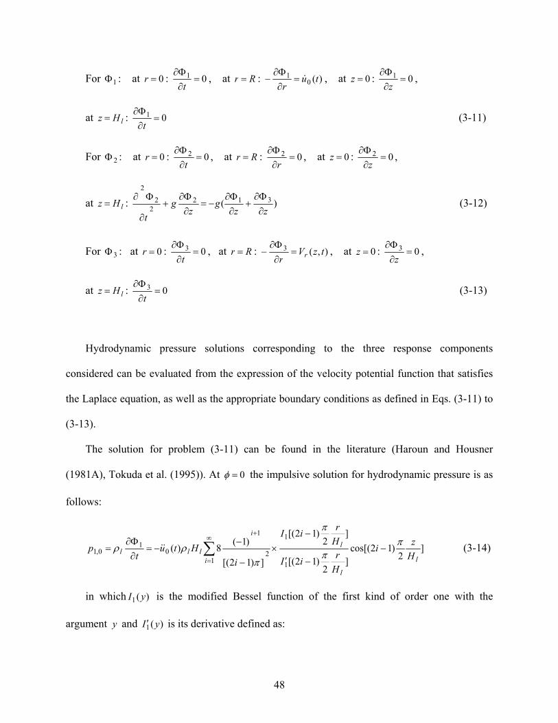
48

For 1 : at 0r : 01 t

, at Rr : )(01 tu

r

, at 0z : 01 z

,

at lHz : 01 t

(3-11)

For 2 : at 0r : 02

t, at Rr : 02

r

, at 0z : 02 z

,

at lHz : )( 3122

2

2

zzg

zg

t

(3-12)

For 3 : at 0r : 03

t, at Rr : ),(3 tzV

r r

, at 0z : 03 z

,

at lHz : 03

t (3-13)

Hydrodynamic pressure solutions corresponding to the three response components

considered can be evaluated from the expression of the velocity potential function that satisfies

the Laplace equation, as well as the appropriate boundary conditions as defined in Eqs. (3-11) to

(3-13).

The solution for problem (3-11) can be found in the literature (Haroun and Housner

(1981A), Tokuda et al. (1995)). At 0 the impulsive solution for hydrodynamic pressure is as

follows:

]2

)12cos[(]

2)12[(

]2

)12[(

])12[(

)1(8)(

11

1

2

1

01

0,1li

l

l

i

lll H

zi

H

riI

H

riI

i

Htut

p

(3-14)

in which )(1 yI is the modified Bessel function of the first kind of order one with the

argument y and )(1 yI is its derivative defined as:

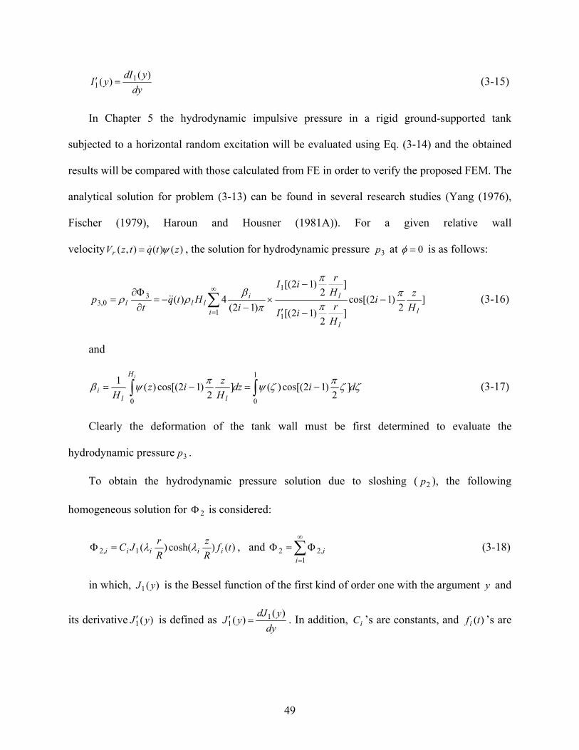
49

dy

ydIyI

)()( 1

1 (3-15)

In Chapter 5 the hydrodynamic impulsive pressure in a rigid ground-supported tank

subjected to a horizontal random excitation will be evaluated using Eq. (3-14) and the obtained

results will be compared with those calculated from FE in order to verify the proposed FEM. The

analytical solution for problem (3-13) can be found in several research studies (Yang (1976),

Fischer (1979), Haroun and Housner (1981A)). For a given relative wall

velocity )()(),( ztqtzVr , the solution for hydrodynamic pressure 3p at 0 is as follows:

]2

)12cos[(]

2)12[(

]2

)12[(

)12(4)(

11

13

0,3li

l

lilll H

zi

H

riI

H

riI

iHtq

tp

(3-16)

and

didzH

ziz

H

lH

lli

1

00

]2

)12cos[()(]2

)12cos[()(1

(3-17)

Clearly the deformation of the tank wall must be first determined to evaluate the

hydrodynamic pressure 3p .

To obtain the hydrodynamic pressure solution due to sloshing ( 2p ), the following

homogeneous solution for 2 is considered:

)()cosh()(1,2 tfR

z

R

rJC iiiii , and

1

,22i

i (3-18)

in which, )(1 yJ is the Bessel function of the first kind of order one with the argument y and

its derivative )(1 yJ is defined as dy

ydJyJ

)()( 1

1 . In addition, iC ’s are constants, and )(tf i ’s are

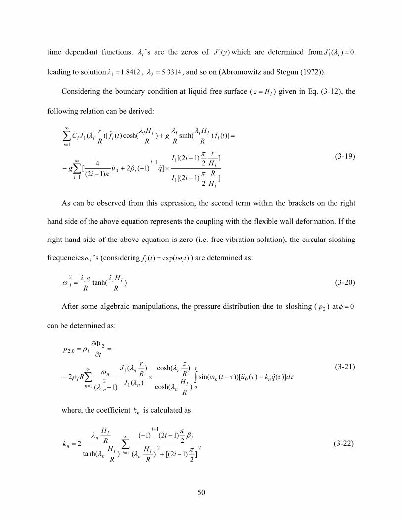
50

time dependant functions. i ’s are the zeros of )(1 yJ which are determined from 0)(1 iJ

leading to solution 8412.11 , 3314.52 , and so on (Abromowitz and Stegun (1972)).

Considering the boundary condition at liquid free surface ( lHz ) given in Eq. (3-12), the

following relation can be derived:

]2

)12[(

]2

)12[(

])1(2)12(

4[

)]()sinh()cosh()()[(

1

11

10

11

l

li

ii

iliili

iii

i

H

RiI

H

riI

qui

g

tfR

H

Rg

R

Htf

R

rJC

(3-19)

As can be observed from this expression, the second term within the brackets on the right

hand side of the above equation represents the coupling with the flexible wall deformation. If the

right hand side of the above equation is zero (i.e. free vibration solution), the circular sloshing

frequencies i ’s (considering )exp()( titf ii ) are determined as:

)tanh(2

R

H

R

g liii

(3-20)

After some algebraic manipulations, the pressure distribution due to sloshing ( 2p ) at 0

can be determined as:

t

o

nnl

n

n

n

n

nn

nl

l

dqkut

R

HR

z

JR

rJ

R

tp

)]()())[(sin()cosh(

)cosh(

)(

)(

)1(

2 01

1

12

20,2

(3-21)

where, the coefficient nk is calculated as

122

1

]2

)12[()(

2)12()1(

)tanh(2

i ln

i

i

ln

ln

n

iR

H

i

R

HR

H

k

(3-22)

51

nk can be computed numerically for the integer variable n and different wall deformation

patterns )( . It can be observed from Eq. (3-21) that the obtained expression for hydrodynamic

pressure due to sloshing ( 2p ) can take into account the effect of the flexible wall displacement

by the term )(qkn . For simplicity, one can define a parameter i as:

]2

)12[(

]2

)12[(

2)12(

1

1

1

l

l

l

i

H

RiI

H

RiI

H

Ri

(3-23)

Finally, using Eqs. (3-14), (3-16), and (3-21), the total hydrodynamic pressure on the tank

wall ( Rr ) at 0 can be evaluated as:

dqkut

R

HR

z

H

zitq

H

zi

itu

R

ppptzp

i

t

ii l

i

i

ii

i

lii

li

i

i

l

Rr

)]()()[(sin

)cosh(

)cosh(

1

]2

)12cos[()(

]2

)12cos[()12(

)1(2)(

2

),(

0

01 12

1

1

0

0,30,20,10

(3-24)

3.2.1.2 Equivalent mechanical model

As mentioned before, generally the fluid hydrodynamic pressure in rigid tanks can be

divided into two distinct parts. One is directly proportional to the ground acceleration and is

caused as a result of fluid motion in unison with the tank. The second is convective pressure

which is due to sloshing at the liquid free surface. As a result, the liquid dynamic behavior inside

closed tanks can be approximated by an equivalent model capable of taking into account the

effects of both liquid components. This equivalence criterion is met by equating the resulting

52

forcers and moments acting on the tank wall between the actual model and its mechanically

equivalent model.

Assuming linear planar liquid motion, an equivalent mechanical model in the form of a

series of mass-spring systems is presented in this section. To develop an equivalent mechanical

model under lateral excitations, the following conditions should be met:

1. The equivalent masses must be maintained.

2. In the case of small oscillations, the center of gravity must remain the same.

3. Models must have the same oscillation modes and must produce the same

damping forces.

4. The resulting forces and moments must be equivalent to those developed in the

actual model.

Figure 3.2 illustrates a schematic diagram of the considered equivalent model. The model

consists of a mass 0m rigidly attached to the tank and moving in unison with the walls, and a

series of masses nm representing the equivalent mass of each sloshing mode. Each mass nm is

fastened to the tank wall by means of a spring nK and a dashpot nC . In the derivation of

equations, for the sake of simplicity, damping is neglected and also only pure translational

excitation is considered here. Furthermore, the tank wall is assumed to be rigid.

As mentioned before, the equivalent model should satisfy the equivalent mass condition as

follows:

1

0n

nmmM (3-25)

where, M is the total mass of fluid.

53

Figure 3.2 Mass-spring-dashpot equivalent mechanical model

In addition, the center of mass must be preserved, therefore:

01

00

n

nnhmhm (3-26)

The spring constants nK for each sloshing mass can be obtained from the equation of

circular sloshing frequencies n ’s. From Eq. (3-20) we have:

)tanh(2

R

H

R

g

m

K lnn

n

nn

(3-27)

Let the displacement of the equivalent masses relative to the tank wall be denoted by nx , and

x be the displacement of the container. The net force acting on the container in the horizontal

direction is determined by adding the reversed inertia forces of the accelerated masses as:

54

Fxxmxm nn

n

)(1

0 (3-28)

Likewise, the slosh equation of the n th mode corresponding to the n th equivalent sloshing

mass can be found as:

02)( nnnnnnnn xmxKxxm (3-29)

where, the term nnnn xm 2 represents the damping force. n is the damping factor of the

equivalent dashpot. The net moment acting on the tank can be determined as:

ynn

nnn

nn Mxxhmxmgxhm

)(11

00 (3-30)

As an example, the special case of harmonic pure lateral excitation of the tank defined as

tXtx sin)( 0 is considered here and the corresponding equations are extracted. 0X and are

the excitation amplitude and frequency. It is assumed no damping is present in the system. As a

result, the slosh equation, Eq. (3-29) takes the form:

tXmxKxm nnnnn sin2

0 (3-31)

The steady state solution for this equation is as follows:

tXx

n

n

sin022

2

(3-32)

The force equation, Eq. (3-28) becomes:

122

22

0

122

2

0

2

01

0

)(1sin

1sin)(

nn

n

nn

nnn

n

M

mtMX

mmtXxxmxmF

(3-33)

The moment equation, Eq. (3-30) becomes:

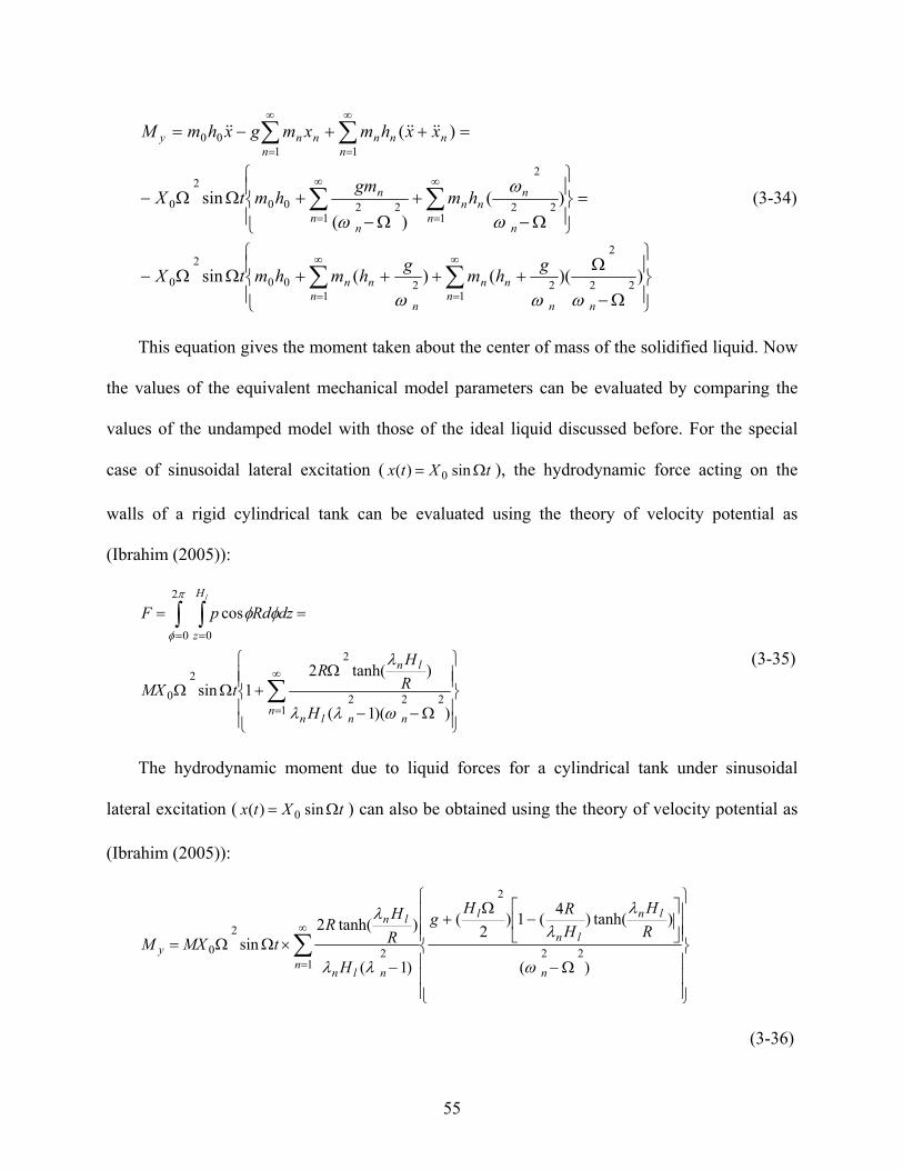
55

1 122

2

2200

2

0

1 122

2

2200

2

0

1100

))(()(sin

)()(

sin

)(

n nnn

nn

n

nn

n nn

nnn

n

n

nn

nnn

nny

ghm

ghmhmtX

hmgm

hmtX

xxhmxmgxhmM

(3-34)

This equation gives the moment taken about the center of mass of the solidified liquid. Now

the values of the equivalent mechanical model parameters can be evaluated by comparing the

values of the undamped model with those of the ideal liquid discussed before. For the special

case of sinusoidal lateral excitation ( tXtx sin)( 0 ), the hydrodynamic force acting on the

walls of a rigid cylindrical tank can be evaluated using the theory of velocity potential as

(Ibrahim (2005)):

1222

2

2

0

0

2

0

))(1(

)tanh(21sin

cos

nnnln

ln

H

z

H

R

HR

tMX

dzRdpFl

(3-35)

The hydrodynamic moment due to liquid forces for a cylindrical tank under sinusoidal

lateral excitation ( tXtx sin)( 0 ) can also be obtained using the theory of velocity potential as

(Ibrahim (2005)):

)(

)tanh()4

(1)2

(

)1(

)tanh(2sin

22

2

12

2

0

n

ln

ln

l

nnln

ln

y

R

H

H

RHg

H

R

HR

tMXM

(3-36)

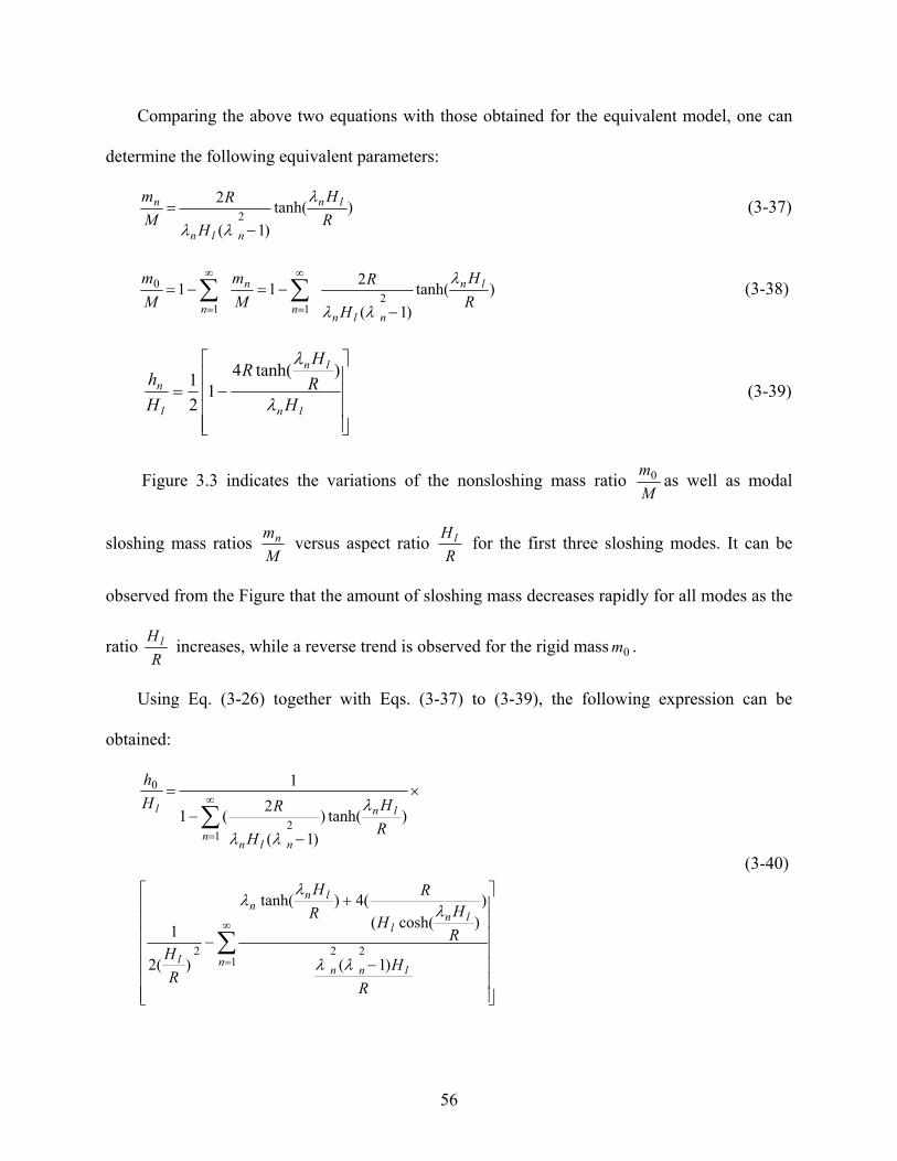
56

Comparing the above two equations with those obtained for the equivalent model, one can

determine the following equivalent parameters:

)tanh(

)1(

22 R

H

H

R

M

m ln

nln

n

(3-37)

)tanh(

)1(

211

211

0

R

H

H

R

M

m

M

m ln

nlnn

n

n

(3-38)

ln

ln

l

n

HR

HR

H

h

)tanh(4

12

1 (3-39)

Figure 3.3 indicates the variations of the nonsloshing mass ratio M

m0 as well as modal

sloshing mass ratios M

mn versus aspect ratio R

Hl for the first three sloshing modes. It can be

observed from the Figure that the amount of sloshing mass decreases rapidly for all modes as the

ratio R

H l increases, while a reverse trend is observed for the rigid mass 0m .

Using Eq. (3-26) together with Eqs. (3-37) to (3-39), the following expression can be

obtained:

1222

12

0

)1(

))cosh((

(4)tanh(

)(2

1

)tanh()

)1(

2(1

1

nlnn

lnl

lnn

l

n

ln

nln

l

R

H

R

HH

R

R

H

R

H

R

H

H

RH

h

(3-40)

57

Figure 3.3 Mechanical model equivalent masses in a circular cylindrical tank

3.3 ACI guidelines for LCS

Based on ACI 350.3-06 (2006), the walls of LCS should be designed for static as well as

dynamic forces. The following dynamic effects should be considered in the design of such

structures:

1. Inertia forces exerted on the wall ( wP ) and the roof ( rP ).

2. Hydrodynamic impulsive force ( iP ) due to accelerated contained liquid.

3. Hydrodynamic convective force ( cP ) due to accelerated contained liquid.

4. Dynamic earth pressure from the supporting soil acting against the buried portion

of the wall.

5. Vertical excitation effects.

R

Hl

M

m0

M

m1

M

m0

M

mn

&

58

These dynamic forces are calculated using the following equations:

i

wiw R

WICP

(3-41)

i

rir R

WICP (3-42)

i

iii R

WICP (3-43)

c

ccc R

WICP (3-44)

where, iC and cC are the period-dependant seismic response coefficients for impulsive and

convective terms, respectively; I is the importance factor as listed in Table 3.1; is effective

mass coefficient defined as the ratio of equivalent dynamic mass of the tank wall to its actual

total mass; wW and rW are the weights of the tank wall and tank roof, respectively; iW and cW

are the effective weights of the stored liquid corresponding to impulsive and convective

components, respectively which are adapted from Housner’s method (Housner (1957; 1963)); iR

and cR are the response modification factors corresponding to impulsive and convective terms,

respectively (see Table 3.2). Since the impulsive and convective terms of response are not in

phase with each other, their effects can be combined using the square-root sum-of-the-squares

(SRSS) method as per ACI 350.3-06.

After hydrodynamic forces iP and cP are determined, they are vertically distributed over the

wall height of the tank in a linear pattern using approximate distribution functions. These

hydrodynamic pressures are distributed horizontally across the tank diameter in a cosine pattern.

One-half the hydrodynamic forces iP and cP are applied symmetrically about 0 acting

outward on one-half of the tank’s circumference. The other half is applied symmetrically about

59

180 acting inward on the opposite half of the tank’s circumference. The wall’s inertia force

should be distributed uniformly around the entire tank’s circumference. Other dynamic effects if

present should be superimposed on these lateral forces in a proper manner.

Table 3.1 Importance factor I (ACI 350.3-06)

Tank use Factor I

III Tanks containing hazardous materials 1.5

II

Tanks that are intended to remain usable for

emergency purposes after an earthquake, or tanks

that are part of lifeline systems

1.25

I Tanks not listed in Categories II or III 1.0

Table 3.2 Response modification factors R (ACI 350.3-06)

Type of structure

iR

cR On or

above

grade

Buried

Anchored, flexible-base tanks 3.25 3.25 1.0

Fixed or hinged-base tanks 2.0 3.0 1.0

Unanchored, contained, or

uncontained tanks 1.5 2.0 1.0

Pedestal-mounted tanks 2.0 ----- 1.0

The schematic vertical and horizontal distribution of these dynamic forces acting on the

walls of a cylindrical tank is shown in Figure 3.4. The impulsive and convective equivalent

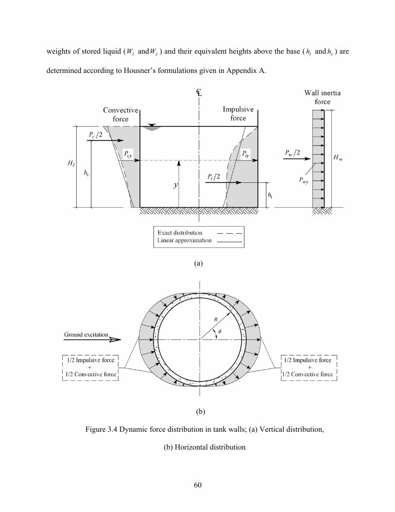
60

weights of stored liquid ( iW and cW ) and their equivalent heights above the base ( ih and ch ) are

determined according to Housner’s formulations given in Appendix A.

(a)

(b)

Figure 3.4 Dynamic force distribution in tank walls; (a) Vertical distribution,

(b) Horizontal distribution

61

The impulsive seismic response coefficient iC is determined as follows:

For sTiT , DSSiC (3-45)

For sTiT , DSSiT

DSiC 1 (3-46)

The convective seismic response coefficient cC is determined as follows as per ACI 350.3-

06:

For sTcT 6.1 , DSS

cTDS

cC 5.115.1 (3-47)

For sTcT 6.1 ,

2

4.2

2

4.06

cT

DSS

cT

DSScC (3-48)

where,

sSaFDSS3

2 = Design spectral response acceleration at short periods

13

21 SvFDS = Design spectral response acceleration at 1-second period

DSSDS

sT 1

iT , cT = Natural period of impulsive mode and convective mode, respectively

SS = Mapped MCE (Maximum Considered Earthquake) spectral response acceleration at

short periods

1S = Mapped MCE spectral response acceleration at 1-second period

aF = Short-period site coefficient (at 0.2 second period)

vF = Long-period site coefficient (at 1.0 second period)

62

The coefficients SS , 1S , aF , and vF are determined in accordance with ASCE 7-05. Figure

3.5 which is adapted from ACI 350.3-06 shows the design response spectrum used in

determining the impulsive seismic response coefficient iC .

Figure 3.5 Design response spectrum (adapted from ACI 350.3-06)

Regarding the dynamic analysis of elevated tanks, additional guidelines are provided in ACI

371R-08. This guide suggests that only the impulsive seismic response coefficient needs to be

considered in determining the seismic induced forces. Therefore, no provisions regarding the

convective component of response are specified in this guide. The design response spectrum is

the same as that provided by ACI 350.3.

3.4 Summary

This chapter addresses the dynamic response of cylindrical liquid storage tanks. It introduces

two different theories commonly used for studying fluid dynamics in liquid containers. It also

explains how velocity potential and as a result hydrodynamic pressures can be determined for a

63

deformable cylindrical tank under a random ground excitation. Using this theory, the analytical

distribution of hydrodynamic pressure on the walls of a cylindrical tank can be computed under

an actual seismic record. This analytical solution will be used later in this thesis to verify the FE

method proposed in this study.

The velocity potential method introduced here enables one to obtain the fluid dynamic

response components due to impulsive action, free surface liquid sloshing, and flexible wall

deformation, separately. The total dynamic effect can therefore be determined by adding up these

three components.

This chapter also summarizes a general procedure for developing the equivalent mechanical

models used in dynamic analysis of liquid tanks. It is worth noting that the mechanical models

introduced here are only applicable to rigid containers supported on rigid foundations. Using

these models, various dynamic responses such as sloshing modes natural frequencies, sloshing

displacement, resultant dynamic shear and overturning moment due to both impulsive and

convective liquid components can be calculated much more simply. These equivalent models

are the basis for most of the current codes and standards dealing with the seismic design of LCS

including ACI 350.3-06. The ACI provisions given in this chapter will be used later in this thesis

to verify the validity of current practice in estimating the seismic response of cylindrical liquid

tanks.

64

CHAPTER 4

FINITE ELEMENT MODELING

4.1 Introduction

In this chapter the fluid-structure interaction problem is formulated using the finite element

(FE) technique. In the previous chapter, basic equations of motion in fluid dynamics were

formulated. The remaining task to be addressed in this chapter is to solve these equations using

an appropriate method capable of accurately simulating the actual behavior of liquid containers

under dynamic loadings. Here, first the general equations of motion are derived for MDOF

structures discretized as systems with a finite number of degrees of freedom. Then, an overview

of how the fluid-structure coupling effect is accounted for in the proposed FE technique along

with the corresponding equations of motion of fluid domain is presented.

In order to obtain the seismic response history of liquid tanks, the discretized structural

equations and the fluid domain equations of motion have to be considered simultaneously as

coupled sets of equations. The main objective of this chapter is to address this issue using FE

method.

This chapter also provides a brief discussion on the problems associated with fluid damping,

and boundary conditions at fluid/structure interface and free surface of the fluid. Moreover, the

element types and meshing patterns used for FE modeling of the tank models are explained. The

general purpose FE analysis software ANSYS® is used for dynamic analysis of liquid tank

models.

65

4.2 Derivation of structural equations of motion

In this section a general formulation is derived for a typical MDOF system subjected to

external forces )(tF j , 1j to n . Consider a classic MDOF system with n degrees of freedom as

shown in Figure 4.1. This classic idealization is very convenient for indicating how the equations

of motion are developed for a typical MDOF system. The forces acting on each accelerated mass

is shown in Figure 4.1 (b). These include the external force )(tF j , the stiffness force SjF , the

damping force DjF , and the inertia force IjF ( 1j to n ).

(a)

(b)

Figure 4.1 (a) Classic MDOF system; (b) Free-body diagrams

66

As shown in the figure, the stiffness and damping forces act in the opposite direction of the

external forces because they are internal forces that resist the exerted motion. Inertial force is

equal to the product of the mass times its acceleration which acts in the opposite direction of

acceleration. From the free-body diagrams and based on the condition of dynamic equilibrium,

for each mass we have:

)(tFFFF jSjDjIj (4-1)

The above equation contains n equations for 1j to n and therefore can be written in

matrix form as:

aSDI FFFF (4-2)

where, aF denotes the applied load vector.

The inertia force vector IF and the acceleration vector u are related through the mass

matrix M as:

uMFI or (4-3)

nnnnjnn

nj

nj

In

I

I

u

u

u

MMMM

MMMM

MMMM

F

F

F

.

.

.

......

....

....

....

......

......

.

.

.2

1

21

222221

111211

2

1

In general, for a lumped mass idealization, the mass matrix is diagonal:

0ijM for ji and jjj MM or 0 (4-4)

The damping force vector DF and the velocity vector u are related through the damping

matrix C as:

67

uCFD or (4-5)

nnnnjnn

nj

nj

Dn

D

D

u

u

u

CCCC

CCCC

CCCC

F

F

F

.

.

.

......

....

....

....

......

......

.

.

.2

1

21

222221

111211

2

1

The stiffness force vector SF and the displacement vector u are related through the

stiffness matrix K as:

uKFS or (4-6)

nnnnjnn

nj

nj

Sn

S

S

u

u

u

KKKK

KKKK

KKKK

F

F

F

.

.

.

......

....

....

....

......

......

.

.

.2

1

21

222221

111211

2

1

We can now write the equations of motion for a MDOF system subjected to external

dynamic forces )(tF j ( 1j to n ) by substituting Eqs. (4-3) to (4-6) into Eq. (4-2):

uM + uC + uK = aF (4-7)

This matrix equation represents n differential equations governing the motion of a MDOF

system subjected to external dynamic forces. The equations are coupled and must be solved

simultaneously.

4.3 Fluid-structure coupling

A fluid-structure interaction problem involves modeling the fluid domain and the

surrounding structure. The interaction of the contained fluid and the structure at an interface

68

causes the hydrodynamic pressure to apply a force exerted on the structure and the structural

motions produce an effective fluid load.

In order to derive the fluid-structure coupling formulations, aF in Eq. (4-7) is separated

into the fluid pressure load acting at the interface preF and resultant of all other forces eF .

Thus, the elemental structural equation can be rewritten as:

ee uM + ee uC + ee uK = pree FF (4-8)

The fluid pressure load vector preF at fluid-structure interface S can be determined by

integrating the pressure over the interface surface area as:

)(SdnpNFS

pre (4-9)

in which,

N is the shape functions used to discretize the structural displacement components

(obtained from the structural element).

p is the fluid pressure.

n is the normal at the fluid boundary.

Using the finite element approximating shape functions for the spatial variation of the fluid

pressure, one can write:

eT pNp (4-10)

where,

N is the shape function for fluid pressure.

ep is the nodal pressure vector.

Substituting Eq. (4-10) into Eq. (4-9) gives:

69

eT

S

pre pSdnNNF )( (4-11)

By definition, the coupling matrix eR relates the pressure of the fluid and the forces on the

fluid-structure interface. Therefore one can write:

eepr

e pRF (4-12)

By comparing the Eqs. (4-11) and (4-12), the coupling matrix is found to be:

)(SdnNNR T

S

Te (4-13)

Finally, the dynamic elemental equation of the structure is obtained by substituting Eq. (4-

12) into Eq. (4-8) as:

ee uM + ee uC + ee uK ee pR = eF (4-14)

4.4 Derivation of fluid finite element formulations

The hydrodynamic pressure distribution throughout the fluid domain is governed by the

pressure wave equation explained in the previous chapter. The following assumptions are made

in deriving the equations:

(1) The fluid is incompressible (density does not change due to pressure variations)

(2) The fluid is inviscid

(3) There is no mean flow of the fluid

(4) The fluid undergoes small-amplitude irrotational motion

Therefore, the wave equation of the fluid system can be written in general three-

dimensional space ),,( zyx as:

0),,,(2

tzyxp (4-15)

70

in which, ),,,( tzyxpp is the hydrodynamic pressure. Since the fluid viscosity is

neglected, the above equation is referred to as the lossless wave equation. In order to accurately

simulate the fluid-structure interaction problem, the discretized structural equation, Eq. (4-7) and

the wave equation, Eq. (4-15) have to be considered simultaneously in finite element

implementation. To discretize the wave equation within fluid domain, first the following matrix

operators (gradient and divergence) are introduced:

zyx

L T. (4-16)

L (4-17)

Therefore, Eq. (4-15) can be rewritten as:

0. p (4-18)

or in matrix notation as:

0)( pLL T (4-19)

The hydrodynamic pressure p in this equation could be due to horizontal and vertical

dynamic excitations of the tank walls and floor. Dynamic motions at these boundaries are related

to the hydrodynamic pressure in fluid domain by defining appropriate boundary conditions along

fluid-structure interfaces as follows:

),,,(),,,(

tzyxan

tzyxpnl

(4-20)

or in matrix notation as:

2

2

..t

unpn l

or (4-21)

71

u

tnpLn T

lT

2

2

)( (4-22)

where,

l is the liquid density.

na is the acceleration component on the boundary along the direction outward normal n .

n is the unit normal to the interface S .

u is the displacement vector of the structure at the interface.

t is time.

In deformable containers na is the sum of the ground acceleration and the wall acceleration

relative to the ground. While, in rigid containers it is obviously equal to the ground acceleration.

Based on the small-amplitude wave assumption on the fluid free surface, one can write the

following boundary condition accounting for the sloshing effects:

01

2

2

z

p

t

p

g (4-23)

where, g is the acceleration due to gravity and z represents the vertical direction. This

equation is the same as Eq. (3-8) but it is written in terms of fluid pressure rather than velocity

potential function. By applying this boundary condition, one can obtain the convective pressure

distribution within the fluid domain.

If only the impulsive component of the fluid response is to be considered, the above-

mentioned boundary condition at fluid free surface should be replaced with the following

boundary condition which imposes zero impulsive pressure at the free surface:

at lHz , 0),,,( tzyxp (4-24)

72

in which, lH is the height of the stored liquid.

Employing the finite element shape functions for the spatial variation of the fluid pressure

p and displacement components u , the following equations can be written:

eT pNp and

eT uNu (4-25)

where,

eu is the nodal displacement component vectors.

N , ep , and N are as defined previously in section 4.3.

Here for simplicity in deriving the equations, the following notation is introduced:

TNLB (4-26)

Finally, using finite element discretization and imposing the previously mentioned boundary

conditions, the discretized wave equation in matrix notation can be found to be:

0 eT

elep

eep

e uRpKpM (4-27)

where,

dANNg

M T

Ae

pe

1 = fluid mass matrix

)(VoldBBKT

Vol

pe = fluid stiffness matrix

)(SdNnNR TT

Se = coupling matrix

In these equations, Ae and Vol represent free surface and volume of the fluid element,

respectively. As mentioned before, S denotes fluid-structure interface.

73

Dissipation of energy due to fluid damping can be accounted for by adding a dissipation

term to the above equation to get:

0 eT

elep

eep

eep

e uRpKpCpM (4-28)

where, peC is the matrix representing the damping in fluid which depends on several

factors such as fluid viscosity, and pressure wave absorption in fluid domain as well as at the

boundaries. This will be further discussed later in this chapter.

Eq. (4-28) together with Eq. (4-14) describe the complete finite element discretized

equations for the fluid-structure interaction problem. These equations can be rewritten in

assembled form as:

00

0

00

e

e

ep

e

fse

e

ep

e

e

e

ep

efse

F

p

u

K

KK

p

u

C

C

p

u

MM

M

(4-29)

in which:

Telfs RM

efs RK

It can be observed from Eq. (4-29) that the coupling matrix eR transfers the structural

acceleration to the fluid domain as well as the fluid pressure to the structure.

In a fluid-structure interaction problem all the submatrices with superscript p in addition to

the coupling submatrices ( fsM and fsK ) are generated by the fluid elements. While all other

submatrices without a superscript are generated by the compatible structural elements used in the

finite element model.

74

The direct integration as well as the modal superposition methods are used to determine the

time history response of the fluid-tank system. Using the direct integration scheme, the

displacement and hydrodynamic pressure values at time increment 1i can be calculated given

the displacement and hydrodynamic pressure at time increment i . In this technique, the step by

step integration is used directly to obtain the solution for the original equations of motion of the

system. During each time step, the structural characteristics are assumed to be constant.

However, these structural properties could differ from one step to another in nonlinear systems

or remain the same during all steps in systems having linear behavior. The modal superposition

method uses the natural frequencies and mode shapes of a linear structure to determine the

response to transient forcing functions.

The accuracy of the time history dynamic solution depends on the integration time step

defined for the solution algorithm. It should be noted that a time step that is too large may cause

errors in the overall response of the system. On the other hand, a time step that is too small

results in time and computer resource wastes. In this study, an integration time step of 0.005

second is used to be small enough to characterize the fluid-structure response in systems with

linear elastic behavior. This was also suggested in various research studies conducted on liquid

containers (Barton and Parker (1987), Mirzabozorg et al. (2003), and Kianoush et al. (2006)). It

is worth noting that the time step of 0.005 second considered for time history dynamic analyses

is smaller than those of recorded ground accelerations used in this study. Moreover, the results of

dynamic analysis using a smaller time step shows that using 0.005 sec as an integration time step

is adequate to provide accurate results.

In the case of nonlinear and/or inelastic systems (seismic isolators in Chapter 8), automatic

time stepping option of ANSYS® program is employed. This option which is also known as time

75

step optimization, automatically adjusts the integration time step during solution according to the

response frequency and the nonlinearity effects. As a result, the program decides when to

increase or decrease the time step during the solution. For systems having nonlinear and/or

inelastic behavior, this feature gives the added advantage of incrementing the loads appropriately

and retreating to the previous converged solution if convergence is not obtained.

4.5 Damping within the fluid domain

Damping is present in most systems including liquid containers and therefore should be

accounted for properly in a dynamic analysis. In fact, damping in liquid tanks depends on several

factors and as a result an accurate evaluation of damping properties of a liquid filled tank is a

difficult task which needs more considerations. However, an appropriate estimation of damping

in such systems can be attained using the classical damping scheme known as Rayleigh damping

(Alpha and Beta damping). Alpha damping and Beta damping are used to define Rayleigh

damping constants and . The damping matrix within the fluid domain peC includes two

components which are due to impulsive and convective parts of the stored fluid:

pe

pe

pe KMC (4-30)

where, peM and p

eK are the mass and stiffness matrices of the fluid element, respectively.

is determined based on the natural frequency of the fundamental sloshing mode and accounts

for the damping due to sloshing on the liquid free surface. is determined based on the

fundamental frequency of the tank and simulates the damping due to the impulsive component.

Eq. (4-30) can be rewritten in the following form:

22i

ii

(4-31)

76

where,

i is the ratio of actual damping to critical damping for a particular mode of vibration, i .

i is the natural circular frequency of mode i .

The natural frequencies corresponding to the fundamental convective and impulsive modes

are obtained through finite element analysis and are used to determine the damping constants

and .

Figure 4.2 shows the schematic variation of Rayleigh damping with respect to damping ratio

and natural circular frequency .

Figure 4.2 Rayleigh damping

As suggested by ACI 350.3-06, the damping ratios of 0.5 and 5 percent are assigned for the

convective and impulsive components, respectively. Furthermore, the stiffness proportional

damping equivalent to 5 and 2 percent of critical damping is assumed as structural damping for

concrete and steel parts of the tank model, respectively.

Damping Ratio ( )

Natural Circular Frequency ( )

Total

Damping

Damping

77

4.6 Finite element models

In this study, two cylindrical ground-supported tanks having different aspect ratios, namely

“Shallow” and “Tall” are modeled using the proposed finite element technique. The tanks are

assumed to be rigidly anchored to the rigid ground. As a result, no sliding or uplift may occur.

The diameters of the tanks are adjusted such that the volume of contained water in both tanks

remains the same. The dimensions and other properties of the tanks are fully explained in the

corresponding chapter of this thesis. The finite element idealizations along with the simplified

geometries of the tanks are shown in Figure 4.3.

The "Shallow" tank is modeled using 2940 fluid elements and 336 shell elements whereas,

4752 fluid elements along with 576 shell elements are employed in FE modeling of the "Tall"

tank. In general, as the mesh size is reduced, that is, as the number of elements is increased, the

accuracy of the solution increases. However, the goal here is to refine the mesh to achieve the

required accuracy by using only as many degrees of freedom as necessary. To illustrate this

point, a study on the FE solution convergence is conducted for rigid “Shallow” and “Tall” tank

models and the resulting FE error is estimated considering different numbers of fluid elements.

The discretization error can be defined as:

100)(

)()((%)

EX

FEEX

p

ppE

(4-32)

Here, the exact analytical solution ( EXp ) based on the Eq. (3-14) explained in Chapter 3 is

used as a baseline solution for error estimation and to provide guidance for mesh revision. The

mesh refinement is continued until the difference between the results obtained from one mesh

and the previously refined mesh becomes negligible.

78

(a)

(b)

Figure 4.3 Ground-supported tank models; (a) "Shallow" tank, (b) "Tall" tank

79

Figure 4.4 is a plot of the resulting error in the impulsive pressure at the bottom of both rigid

“Shallow” and “Tall” tank models versus the number of fluid elements. As obvious from the

Figure, error percentages of around 1.63% and 1.9% are found for “Shallow” and “Tall” models,

respectively assuming the number of elements mentioned above. The time history variation of

impulsive pressure is obtained for the considered tank models under the horizontal component of

1940 El-Centro record scaled to the peak ground acceleration of 0.4g. The obtained

discretization errors are within the acceptable range typically observed in numerical simulations.

Further details on the comparison of analytical and FE results will be provided later in Chapter 5.

-60

-50

-40

-30

-20

-10

0

0 1500 3000 4500 6000

Number of fluid elements

Pe

rce

nt

err

or

in p

res

su

re a

t th

e b

ott

om

of t

he

tan

k

Exact solution

-60

-50

-40

-30

-20

-10

0

0 1500 3000 4500 6000 7500

Number of fluid elements P

erc

en

t e

rro

r in

pre

ss

ure

at

the

bo

tto

m o

f th

e t

an

k

Exact solution

(a) (b)

Figure 4.4 Inaccuracy of FE solution as a function of the number of fluid elements;

(a) Shallow tank, (b) Tall tank

A typical finite element idealization of an elevated tank model investigated in this study is

indicated in Figure 4.5. Shown in the figure is also the simplified geometry of the tank. The total

number of elements used for finite element modeling of the tank varies depending on the tank

geometric properties. Full details regarding the finite element modeling of each specific elevated

tank under consideration is provided in the corresponding sections of the thesis.

80

Figure 4.5 Typical elevated tank model

In finite element modeling, tank walls as well as all other structural parts including the

supporting shaft in elevated tanks are modeled using four-node quadrilateral shell elements. The

element has six degrees of freedom (translations in the nodal x, y, and z directions and rotations

about the nodal x, y, and z axes) at each node and both bending and membrane behaviors are

permitted. The geometry, node locations, and the coordinate system for this element are shown

in Figure 4.6. As shown in the figure, a triangular-shaped geometry is also available for this

element. Both normal and in-plane loads are allowed. Pressures may be applied as surface loads

on the faces of the element as indicated by the circled numbers in Figure 4.6 (a). Shear deflection

is not included in this thin-shell element. In this study, fluid domain is modeled using eight-node

isoparametric brick fluid elements in a three dimensional space. Two different types of fluid

elements; displacement-based (D-Fluid), and pressure-based (P-Fluid) elements are used for

finite element modeling of the fluid through out this research.

81

(b) (c)

Figure 4.6 Finite elements geometries; (a) Shell element, (b) P-Fluid, (c) D-Fluid

The finite element formulation of P-Fluid elements is described previously in section 4.4. P-

Fluid elements used in this study have eight corner nodes with four degrees of freedom per node:

translations in the nodal x, y, z directions and pressure. The translational degrees of freedom are

only needed for nodes located on the interface. Figure 4.6 shows the geometry, node locations,

and the coordinate system for this element. As shown in the figure, prism-shaped and

tetrahedron-shaped geometries are also available for this element. Fluid-structure interfaces (FSI)

can be flagged by surface loads at the element faces as indicated by the circled numbers in

(a)

82

Figure 4.6. By defining the FSI on desired element faces, the structural motion and fluid pressure

at the interface will be coupled.

D-Fluid elements used in this study have eight corner nodes with three degrees of freedom

per node: translations in the nodal x, y, z directions. The element is capable of accounting for

fluid-structure interactions. Acceleration effects, such as in sloshing problems may be considered

using this element. Fluid elements at a boundary should be coupled with the structural elements

in the direction normal to the interface. The geometry, node locations, and the coordinate system

for this element are shown in Figure 4.6. The finite element formulation of D-Fluid elements is

described in the following section.

4.7 D-Fluid finite element formulation

D-Fluid elements use displacements as the variables in the fluid domain. These elements are

considered as an extension of structural solid elements in which the element shear modulus is set

to zero and the fluid bulk modulus K is used to establish the elastic stress-strain relations. D-

Fluid elements are particularly useful in modeling fluids contained within vessels having no net

flow rate and can be employed for transient as well as free vibration analyses. The stress-strain

relationship of the element is established using the stiffness matrix as follows:

z

y

x

xz

yz

xy

z

y

x

xz

yz

xy

bulk

M

M

M

P

B

B

B

S

S

S

K

R

R

R

/1000000

0/100000

00/10000

000/1000

0000/100

00000/10

000000/1

(4-33)

where, z

w

y

v

x

ubulk

= bulk strain

83

K = fluid elastic (bulk) modulus

P = pressure

= shear strain

S = K x 10-9 (arbitrarily small number to give element some shear stability)

= shear stress

iR = rotation about axis i

B = K x 10-9 (arbitrarily small number to give element some rotational stability)

iM = twisting force about axis i

Damping matrix of the element that relates the strain rates (strain differentiation with respect

to time) to the stresses can also be defined as:

z

y

x

xz

yz

xy

z

y

x

xz

yz

xy

bulk

M

M

M

P

C

C

C

R

R

R

/1000000

0/100000

00/10000

000/1000

0000/100

00000/10

0000000

(4-34)

where, = viscosity, and C = .00001

The element does not generate a consistent mass matrix and only the lumped mass matrix is

available. The sloshing effects and associated mode characteristics can be studied using this

element. To hold the free surface in place, springs having the equivalent stiffness sK are added to

each node of the element. sK is determined as follows:

)( zCzgyCygxCxgfAsK l (4-35)

84

where, l = liquid density, fA = area of the face of the element, ig = acceleration in the i

direction, and iC = ith component of the normal to the face of the element. Added springs have

positive constants at the nodes on top of the element and have negative constants for those

located on bottom surface. Hence, at the interior nodes within the liquid domain, these effects

cancel out and they only operate at the fluid free surface.

4.8 Summary

The equation of motion for a typical structural MDOF system subjected to external dynamic

forces was derived. The procedure for coupling the fluid and structural domains in finite element

modeling of the liquid tanks was discussed. The coupling matrix transferring the structural

motion and the hydrodynamic pressure between the structure and the fluid was developed.

The finite element formulation for the coupled system of liquid tanks in the time domain

was described. In deriving these formulations, appropriate boundary conditions available in

typical liquid tanks were applied. In addition, problems associated with damping characteristics

of the fluid domain were discussed. Using the proposed finite element technique, the effects of

both impulsive and convective parts and their corresponding damping effects can be taken into

account. The proposed technique is general and can be employed for any tank configurations, or

any direction of seismic excitation. This method can account for all aspects of structural and

fluid components in the time domain.

Some important properties of the elements used in this study for finite element modeling of

both ground-supported and elevated tank models were described in this chapter.

85

CHAPTER 5

DYNAMIC RESPONSE OF CYLINDRICAL GROUND-SUPPORTED

TANKS

5.1 Introduction

This chapter deals with the dynamic behavior of cylindrical open top ground-supported

water tanks. The main focus of this chapter is to identify the factors having significant effects on

the dynamic response of such structures and to address the interaction between these parameters.

Examined parameters are sloshing of liquid free surface, tank wall flexibility, vertical ground

acceleration, tank aspect ratio, and base fixity. To accurately investigate the dynamic behavior of

the tanks, the hydrodynamic response is divided into impulsive and convective components.

In addition, the dynamic results obtained from the rigorous finite element method are

compared with those recommended by current practice and thereby the adequacy of current code

provisions in estimating the dynamic response of liquid-filled cylindrical containers is

investigated. The validity of the proposed finite element method is verified by comparing the

results with those calculated from well-proved analytical methods available in the literature.

In the first part of this Chapter, two rigid cylindrical tanks having different aspect ratios are

modeled in three-dimensional space and their free vibration results are compared with those

obtained through analytical approaches.

Time history response of both rigid and flexible tanks having different conditions at the

base; fixed and hinged under both horizontal and vertical components of earthquake is obtained

using the direct integration method. Based on the computed results, important conclusions

86

regarding the seismic behavior of cylindrical ground-supported tanks are drawn and some

suggestions to be considered in seismic design of liquid containers are made.

5.2 Tank models properties

Two cylindrical concrete tank models with different aspect ratios, representative of two

classes of tanks namely "Shallow" and "Tall" are considered for finite element analysis

throughout this chapter. Some information regarding the finite element modeling and geometric

properties of the tanks is provided in section 4.6. Dimensions of the tanks are shown in Figure

4.3 and are selected such that the volume of stored water remains unchanged for both tank

models. The tanks are assumed to be rigidly anchored to the rigid ground. As a result, the effect

of soil-structure interaction is not included. Since only anchored tanks are considered, the tank

floor is not included in the FE model. The tank walls are considered to be of constant thickness

and connected to the base such that no sliding or uplift may occur.

The tank structure is modeled using elastic shell elements and the fluid domain is modeled

using 3D brick-shaped fluid elements. Properties of the concrete and water materials are as

follows:

Concrete Water

Density = 2400 kg/m3

Young’s modulus = 24.86 GPa

Poisson’s ratio = 0.16


Considered tanks have the aspect ratios of 115.0D

Hl (Shallow tank), and 324.0D

Hl

(Tall tank), where lH and D are as indicated in Figure 4.3. The finite element idealizations of

the tanks are also shown in Figure 4.3.

87

Fluid and shell domains should be meshed in such a way that the location of each node of

the fluid domain on the interface coincide exactly with that of the corresponding shell element.

Then, these coincident nodes must be coupled in order to get equal displacements in radial

direction for both fluid and shell nodes located on the interface. However, tangential relative

displacements should be possible to happen. Fluid nodes should be coupled at all interfaces with

containing structure; as a result all fluid nodes located at the interface with the tank floor must be

restrained in vertical direction.

5.3 Free vibration analysis

Prior to performing time history analysis, free vibration analysis is carried out on the tank

models assuming rigid wall boundary condition. The tanks are assumed to have the fixed

boundary condition at the base. The natural frequencies and modal responses are obtained using

both FE and analytical methods for impulsive and convective modes with the highest

participation factors among all modes of vibration.

For each model, the fundamental mode is identified as that with the largest participation

factor (β) in the horizontal X direction. Table 5.1 shows computed results determined through FE

analysis along with those obtained from analytical methods.

The method introduced by Housner (1963) is used here as an analytical approach for

calculating the natural frequency of the fundamental sloshing mode as well as the impulsive and

convective mass ratios. Since Housner's method is only applicable to tanks with rigid wall

boundary condition, tank models considered in this section are assumed to be rigid as well. A

detailed description on Housner’s method along with all relevant formulations are given in

Appendix A.

88

Table 5.1. Free vibration analysis results for ground-supported rigid tank models

"Shallow" Model

Mode Frequency (Hz) Effective mass

(FE) (kN.s2/m)

Ri (%) β

(normalized) Number type FE Analytical FE Analytical

*1 C

onve

ctiv

e 0.087 0.087 7790.1 78.8 79.8 1.00

2 0.216 NA 457.6 4.6 NA 0.25

*1

Impu

lsiv

e 39.410 38.00 1290.7 13.1 13.3 0.40

2 79.670 NA 20.0 0.2 NA 0.05

"Tall" Model

Mode Frequency (Hz) Effective mass

(FE) (kN.s2/m)

Ri (%) β

(normalized) Number type FE Analytical FE Analytical

*1

Con

vect

ive 0.149 0.149 5779.0 58.0 59.0 1.00

2 0.277 NA

197.9 2.0 NA

0.18

3 0.350 39.3 0.4 0.08

*1

Impu

lsiv

e 30.530 36.00 3537.2 35.5 37.0 0.78

2 61.780 NA

111.4 1.1 NA

0.14

3 74.060 43.9 0.4 0.09

* Fundamental mode.

The analytical method proposed by Veletsos and Shivakumar (1997) is used to determine

the fundamental impulsive frequency of the tank-liquid system as:

cc

lIi

gE

HC

3

101

(5-1)

R

tCC w

wI 10 (5-2)

iii f

T12

(5-3)

where:

89

IC and wC : coefficients for determining the fundamental frequency of the tank-liquid

system

lH : depth of stored liquid (m)

cE : modulus of elasticity of concrete (MPa)

g : acceleration due to gravity (9.807 m/s2)

c : density of concrete (kN/m3)

wt : average wall thickness (mm)

R : inside radius of the tank (m)

i : circular frequency of the fundamental impulsive mode of vibration (radian/s)

if : natural frequency of the fundamental impulsive mode of vibration (Hz)

For :667.0lH

D (5-4)

52

4322

)(10186.3

)(1267.0)(1253.0)(1034.0)(2039.010375.9

D

HD

H

D

H

D

H

D

HC

l

llllw

or, alternatively wC can be determined from Figure 5.1. These two analytical methods

(Housner (1963) and Veletsos and Shivakumar (1997)) are also adapted by ACI 350.3-06 for

determining the dynamic characteristics of ground-supported concrete cylindrical tanks.

The ratio (Ri) of the effective modal mass in X direction to the total mass of the system for

each mode under consideration is also included in Table 5.1. Since the tank wall is modeled as

massless shell elements, the obtained modal masses are only contributed by the contained fluid.

Therefore, the results obtained from FE analysis are readily comparable with those computed

from Housner's method.

90

Figure 5.1 Coefficient wC for ground-supported cylindrical tanks

(adapted from ACI 350.3-06)

The modal participation factors (β) normalized with respect to their largest values for each

model are also given in the table. The participation factor corresponding to a specific mode

denoted as fundamental mode is much greater than those of other modes. This implies that the

response of the system is dominated by these modes when excited horizontally in X direction.

For instance, Ri for the first convective mode of the "Tall" model is 96% of the total Ri

obtained by adding those of the three convective modes considered. Regarding the impulsive

response of the "Tall" tank, this ratio is again around 96%. The same trend is observed for the

"Shallow" tank. Therefore, for practical purposes, only the fundamental impulsive and

convective modes (mode numbers 1 in the table) need to be taken into account in order to

estimate the dynamic response of such tanks under horizontal excitations.

91

It is worth noting that all impulsive modes contributing the most to the response to

horizontal excitation are cantilever beam type modes with circumferential wave number (n)

equal to 1 in which shell cross section remains circular while vibrating.

Results of free vibration analyses show that the participation factors and effective masses

associated with the cos(nθ) type modes (n > 1) are very small and therefore can be neglected in

determining the response to horizontal excitations. This has also been stated by Barton and

Parker (1987) for cylindrical tanks having height/diameter ratio larger than 0.5 and also by El

Damatty et al. (2005) for conical tanks.

It is important to note that in FE analysis, the tanks can not be modeled as infinitely rigid.

This will cause singularity in the solution process. Therefore, the tanks are made relatively rigid

by introducing a very large modulus of elasticity for shell material. A Young's modulus of ten

times greater than that of a normal concrete is assigned to the shell elements to account for the

effect of tank wall rigidity. As a result, as can be observed from Table 5.1, very large impulsive

natural frequencies implying the relative rigidity of the tank walls are obtained for FE models.

Considering the wall thicknesses of 300 and 500mm for "Shallow" and "Tall" tanks,

respectively, one can use Eqs. (5-1) to (5-4) to compute the natural frequencies of the

fundamental impulsive modes. As a result, the fundamental impulsive frequencies of 38 and 36

Hz are calculated for "Shallow" and "Tall" tanks, respectively, which are in close agreement with

those obtained from FE.

The mode shapes of "Tall" model listed in Table 5.1 are displayed in Figure 5.2. The

sloshing profiles for the first three convective modes of cylindrical containers given by Veletsos

(1984) are also shown in the figure. Comparing these two sets of sloshing mode shapes, it is

92

obvious that they are quite similar in terms of the radial distribution of vertical displacements at

liquid free surface.

(a)

(b)

(c)

Figure 5.2 Mode shapes of "Tall" model (horizontal motion); (a) First three convective modes

(FE), (b) First three convective modes (adapted from Veletsos (1984)), (c) First three impulsive

modes (FE)

Comparing the FE and analytical results given in Table 5.1, it can be observed that the finite

element results are in excellent agreement with those calculated through analytical approaches

verifying that the proposed FE model can be employed with high accuracy to study the fluid-

93

structure interaction problems of liquid containing structures. A relatively better agreement

between results is found for the convective term as compared to the impulsive term especially in

terms of the fundamental natural frequencies. The reason could be due to the fact that in both FE

and Housner’s formulations, the linearized wave equation is employed.

5.4 Verification of numerical model

To further verify the proposed FE technique, the hydrodynamic response of the “Shallow”

tank under random seismic excitation is obtained using the FE technique and the results are

compared with the analytical solution proposed by Haroun and Housner (1981A). The

considered tank is assumed to have fixed condition at the base. Tank walls are assumed to be

rigid, and the tank floor is fully anchored to the rigid ground. For comparison purposes, zero

damping is assumed for the system.

The horizontal component of 1940 El-Centro earthquake scaled to the peak ground

acceleration of 0.4g is used as an excitation and the time history response of the tank-liquid

system is obtained. Based on Haroun’s study, the analytical impulsive pressure for a rigid

cylindrical tank can be obtained using Eq. (3-14) described in detail in Chapter 3. For

convenience the equation is rewritten here in the following form:

1 1

21

10

1 )cos()cos()(

)()1()(2),,,(

ii

ii

ii

l

l zRI

RI

H

tutzRp

(5-5)

where:

i are constants given by l

i H

i

2

)12( (5-6)

and z are circumferential and axial coordinates, respectively with the center of the base

being the origin.

94

R = tank radius

l = liquid mass density

)(0 tu = horizontal ground acceleration

lH = liquid depth

1I = modified Bessel function of the first kind of order 1 and 1I is its derivative.

In calculating the hydrodynamic pressure by Eq. (5-5), the first fifteen terms of the series

( 1i to 15) are used. More series terms may be included in order to obtain results of higher

accuracy. However, for the tank model under consideration, an excellent estimation of the

hydrodynamic pressure is obtained using the first fifteen terms. The hydrodynamic impulsive

pressure distribution over the height of the rigid tank calculated through analytical solution and

FE is shown in Figure 5.3. The impulsive pressure time history at the bottom of the tank adjacent

to the wall ( ,Rr ,0 0z ) is also shown in Figure 5.4. It is obvious that FE and analytical

results are in excellent agreement. This further verifies the validity of the proposed FE technique.

0

1

2

3

4

5

6

0 5 10 15 20

Pressure (kPa)

Hei

gh

t (m

)

Analytical

FE_Zero damping

Figure 5.3 Impulsive pressure distribution over the height of the rigid “Shallow” tank

95

-20

-15

-10

-5

0

5

10

15

20

0 5 10 15 20

Time (s)

Pre

ssu

re (

kPa)

FE

Analytical

Figure 5.4 Time history of impulsive pressure at ( ,Rr ,0 0z )

5.5 Effect of tank wall flexibility and vertical earthquake component

In order to study the effect of tank wall flexibility, the time history response of tank models

having both rigid and flexible walls are calculated and a comparison between the obtained results

is made. Furthermore, to investigate the effect of vertical component of earthquake on dynamic

behavior of cylindrical tanks, the seismic response of the tanks under both the horizontal

component alone and the combined horizontal and vertical components are obtained. In

performing the time history analyses, the horizontal and vertical components of 1940 El-Centro

earthquake are used as seismic excitations. The components are scaled in such a way that the

peak ground acceleration in the horizontal direction reaches 0.4g. The scaled earthquake

components are shown in Figure 5.5. The tanks considered in this section are assumed to have

hinged boundary condition at their base.

96

-0.5-0.4-0.3-0.2-0.1

0

0.10.20.30.40.5

0 10 20 30 40

Time (Sec)

Acc

eler

atio

n (

g)

-0.5-0.4-0.3

-0.2-0.1

00.10.2

0.30.40.5

0 10 20 30 40

Time (Sec)

Acc

eler

atio

n (

g)

(a) (b)

Figure 5.5 Scaled 1940 El-Centro earthquake; (a) Horizontal component,

(b) Vertical component

5.5.1 Dynamic behavior of rigid tanks

(a) Shallow tank

The total time history response of the tanks is separated into impulsive and convective

components in order to study the time varying response characteristics of the tank models. The

examined responses include the hydrodynamic pressure exerted by the liquid on the tank wall;

the associated structural forces including the hoop force, bending moment, and shear force; and

the vertical displacement or sloshing height of the liquid free surface.

The transient hoop force, bending moment, and shear force responses for the rigid

“Shallow” tank under the horizontal component of El-Centro earthquake are obtained and

indicated in Figure 5.6. The structural responses are reported at the locations of maximum

response within the tank wall and are calculated per unit width of the wall. The maximum shear

occurs at the base of the wall; therefore it will be referred to as base shear. However, for a hinged

tank, the maximum hoop force and bending moment occur far from the base and around the mid

height of the tank wall.

97

‐4.0E+05

‐3.0E+05

‐2.0E+05

‐1.0E+05

0.0E+00

1.0E+05

2.0E+05

3.0E+05

4.0E+05

0 5 10 15 20 25 30 35 40 45 50 55 60

Time(S)

Hoop Force (N/m

) Convective

Impulsive

Accel: H

(a)

‐2.0E+04

‐1.5E+04

‐1.0E+04

‐5.0E+03

0.0E+00

5.0E+03

1.0E+04

1.5E+04

2.0E+04

0 5 10 15 20 25 30 35 40 45 50 55 60

Time(s)

Mom

ent (N.m

/m) Convective

Impulsive

Accel: H

(b)

‐3.0E+04

‐2.0E+04

‐1.0E+04

0.0E+00

1.0E+04

2.0E+04

3.0E+04

0 5 10 15 20 25 30 35 40 45 50 55 60

Time(s)

Base shear (N/m

)

Convective

Impulsive

Accel: H

(c)

Figure 5.6 Time history response of the rigid “Shallow” tank due to horizontal excitation;


98

The absolute maximum values for the impulsive hoop force, moment, and base shear due to

horizontal excitation are 326 kN/m, 15.2 kNm/m, and 20.2 kN/m, respectively. The

corresponding absolute peak values of convective hoop force, moment, and base shear are 109

kN/m, 4.9 kNm/m, and 6.5 kN/m, respectively. As can be observed from Figure 5.6, the

impulsive and convective response components do not reach their peaks at the same time.

Furthermore, by comparing the convective response values with those of impulsive response, one

can conclude that the forces resulting from liquid sloshing have less significant effect on the

dynamic response of the liquid-tank system.

Table 5.2 summarizes the peak response values calculated through time history FE analysis.

The time history diagram for sloshing of water free surface is shown in Figure 5.7. The sloshing

response is reported at ,0 adjacent to the tank wall. The maximum positive sloshing height of

248 mm occurs at t = 40.86 sec as a result of horizontal excitation. The peak value of sloshing

height occurs far after the peak of the ground acceleration. ACI 350.3-06 predicts the maximum

sloshing height of 440 mm which is well above the FE result and is suitable in terms of providing

sufficient design freeboard between the water free surface and the roof.

99

Table 5.2 Summary of peak time history analysis results

Hoop Force (N/m) ×103

Moment (N.m/m) ×103

Base Shear (N/m) ×103

Sloshing (mm)

Rigid

Shallow Impulsive H 326 15.2 20.2 NA

Convective H 109 4.9 6.5 248

Tall Impulsive H 685 35.6 47.1 NA

Convective H 212 10.9 14.4 931

Flexible

Shallow

Impulsive

H 613

88% 27.1 78%

33.9 68%

NA

H+V 652 28.2 35.0 NA

(H+V)/H 1.06 1.04 1.03 NA

Convective

H 98

-10% 4.7

-4% 6.1

-6% 243 -2%

H+V 105 5.0 6.5 253

(H+V)/H 1.07 1.06 1.07 1.04

Tall

Impulsive

H 1331 94%

60.3 69%

73.1 55%

NA

H+V 1558 75.1 92.9 NA

(H+V)/H 1.17 1.24 1.27 NA

Convective

H 201 -5%

10.1 -7%

13.1 -9%

894 -4%

H+V 239 12.7 16.9 965

(H+V)/H 1.19 1.26 1.29 1.08

‐400

‐300

‐200

‐100

0

100

200

300

400

0 5 10 15 20 25 30 35 40 45 50 55 60

Time(s)

Sloshing (m

m)

Accel: H

Figure 5.7 Sloshing height time history for rigid “Shallow” tank due to horizontal excitation

100

(b) Tall tank

The transient hoop force, bending moment, and base shear responses for the rigid “Tall”

tank model are shown in Figure 5.8. The absolute maximum values of the resulting hoop force,

moment, and base shear corresponding to the impulsive component due to horizontal excitation

are 685 kN/m, 35.6 kNm/m, and 47.1 kN/m, respectively. The calculated absolute maximum

values of convective hoop force, moment, and base shear are 212 kN/m, 10.9 kNm/m, and 14.4

kN/m, respectively which occur at about 3.1 seconds after peaks of impulsive response. The

ratios of convective maximum response values to the corresponding impulsive values are found

to be higher in “Shallow” tank as compared to “Tall” tank. This implies that the convective

component has somewhat more significant effect on the overall dynamic response of liquid-tank

systems in shallow containers compared to tall containers.

The time history of sloshing height at water free surface adjacent to the wall is given in

Figure 5.9. Due to horizontal excitation, the maximum positive sloshing height of 931mm occurs

at t = 25.14 sec. According to ACI 350.3-06, the design sloshing height of 910mm is obtained

which is very close to the calculated FE value.

101

‐8.0E+05

‐6.0E+05

‐4.0E+05

‐2.0E+05

0.0E+00

2.0E+05

4.0E+05

6.0E+05

8.0E+05

0 5 10 15 20 25 30 35 40 45 50 55 60Time(s)

Hoop Force (N/m

)

Convective

Impulsive

Accel: H

(a)

‐4.0E+04

‐3.0E+04

‐2.0E+04

‐1.0E+04

0.0E+00

1.0E+04

2.0E+04

3.0E+04

4.0E+04

0 5 10 15 20 25 30 35 40 45 50 55 60

Time(s)

Moment (N.m/m

)

Convective

Impulsive

Accel: H

(b)

‐6.0E+04

‐4.0E+04

‐2.0E+04

0.0E+00

2.0E+04

4.0E+04

6.0E+04

0 5 10 15 20 25 30 35 40 45 50 55 60

Time(s)

Base Shear (N/m

) ConvectiveImpulsive

Accel: H

(c)

Figure 5.8 Time history response of the rigid “Tall” tank due to horizontal excitation;


102

‐1200

‐900

‐600

‐300

0

300

600

900

1200

0 5 10 15 20 25 30 35 40 45 50 55 60Time(s)

Sloshing (m

m)

Accel: H

Figure 5.9 Sloshing height time history for rigid “Tall” tank due to horizontal excitation

5.5.2 Dynamic behavior of flexible tanks

(a) Shallow tank

The FE time history results for “Shallow” and “Tall” tank models with flexible wall

boundary condition due to both horizontal and combined horizontal and vertical excitations are

also presented in Table 5.2. The numbers in bold in the table show an increase (positive) or

decrease (negative) percentage over the corresponding rigid tank model. The transient structural

responses for flexible “Shallow” tank model are shown in Figure 5.10 and 5.11.

Due to horizontal excitation, the absolute maximum values of hoop force, moment, and base

shear are 613 kN/m, 27.1 kNm/m, and 33.9 kN/m, respectively for impulsive component and 98

kN/m, 4.7 kNm/m, and 6.1 kN/m for convective component. As compared to the results obtained

for the rigid tank, it can be observed that maximum values of impulsive hoop force, moment, and

base shear are increased considerably by 88, 78, and 68 percents, respectively as a result of wall

flexibility effect. On the other hand, the obtained results indicate only a negligible decrease in

associated convective response values due to the flexibility of tank walls. This shows that the

convective part of response is almost independent of tank wall flexibility.

103

‐8.0E+05

‐6.0E+05

‐4.0E+05

‐2.0E+05

0.0E+00

2.0E+05

4.0E+05

6.0E+05

8.0E+05

0 5 10 15 20 25 30 35 40 45 50 55 60

Time(s)

Hoop Force (N/m

) Convective

Impulsive

Accel: H

(a)

‐4.0E+04

‐3.0E+04

‐2.0E+04

‐1.0E+04

0.0E+00

1.0E+04

2.0E+04

3.0E+04

4.0E+04

0 5 10 15 20 25 30 35 40 45 50 55 60Time(s)

Mom

ent (N.m

/m) Convective

Impulsive

Accel: H

(b)

‐6.0E+04

‐4.0E+04

‐2.0E+04

0.0E+00

2.0E+04

4.0E+04

6.0E+04

0 5 10 15 20 25 30 35 40 45 50 55 60Time(s)

Base shea

r (N/m

) Convective

Impulsive

Accel: H

(c)

Figure 5.10 Time history response of the flexible “Shallow” tank due to horizontal


104

‐8.0E+05

‐6.0E+05

‐4.0E+05

‐2.0E+05

0.0E+00

2.0E+05

4.0E+05

6.0E+05

8.0E+05

0 5 10 15 20 25 30 35 40 45 50 55 60

Time(s)

Hoop

Force (N/m

) Convective

Impulsive

Accel: H+V

(a)

‐4.0E+04

‐3.0E+04

‐2.0E+04

‐1.0E+04

0.0E+00

1.0E+04

2.0E+04

3.0E+04

4.0E+04

0 5 10 15 20 25 30 35 40 45 50 55 60

Time(s)

Moment (N.m

/m) Convective

Impulsive

Accel: H+V

(b)

‐6.0E+04

‐4.0E+04

‐2.0E+04

0.0E+00

2.0E+04

4.0E+04

6.0E+04

0 5 10 15 20 25 30 35 40 45 50 55 60

Time(s)

Base shea

r (N/m

) Convective

Impulsive

Accel: H+V

(c)

Figure 5.11 Time history response of the flexible “Shallow” tank due to combined

horizontal and vertical excitation; (a) Hoop force, (b) Moment, (c) Base shear

Considering the combined effect of horizontal and vertical excitations, it can be observed

from the table that the impulsive hoop force, moment, and base shear slightly increase by about

105

6, 4, and 3 percent, respectively. As compared to the impulsive response, the corresponding

convective values increase somehow more drastically by about 7, 6, and 7 percent, respectively.

Therefore, it can be concluded that the vertical ground acceleration has a stronger effect on the

convective part of response than it has on the impulsive part. It is also found that the effect of

vertical ground motion on overall seismic response of the “Shallow” tank model is insignificant.

As a result of vertical acceleration, the peak value of sloshing is increased from 243mm at t

= 40.86 sec to 253mm at t = 5.78 sec which shows an increase of around 4 percent compared to

the case of horizontal excitation alone. The time history variation of sloshing height is shown in

Figure 5.12. Comparing the calculated sloshing height for the flexible tank with that of rigid

tank, a reduction of around 2 percent is observed due to the effect of wall flexibility.

‐400

‐300

‐200

‐100

0

100

200

300

400

0 5 10 15 20 25 30 35 40 45 50 55 60Time(s)

Sloshing (m

m)

H

H+V

Figure 5.12 Sloshing height time history for flexible “Shallow” tank

The hydrodynamic pressure distribution over the height of the tank wall for both rigid and

flexible tank models under horizontal excitation is shown in Figure 5.13. To examine the

adequacy of current practice in estimating the hydrodynamic response of liquid-filled cylindrical

tanks, the hydrodynamic pressure distribution recommended by ACI 350.3-06 is also indicated in

106

the figure. It is worth noting that the ACI hydrodynamic pressure values are calculated assuming

I = 1 and R = 1, where I is the ‘‘Importance factor’’ and R is the ‘‘Response modification

coefficient’’. For Code calculations, the design spectrum with a peak ground acceleration of 0.4g

to correspond with the horizontal seismic excitation used in FE analyses is used. The mapped

spectral accelerations ( sS and 1S ) of 1.5 g and 0.6 g, respectively are selected for Imperial

Valley location. Moreover, a site with hard rock soil which is categorized as site class “A” as per

ASCE 7-05 is assumed in the Code calculations. In obtaining the results based on ACI 350.3-06,

the damping ratios of 0.5% and 5% are assumed for convective and impulsive components,

respectively.

0

1

2

3

4

5

6

0.E+00 1.E+04 2.E+04 3.E+04 4.E+04 5.E+04 6.E+04

Maximum Hydrodynamic Pressure (Pa)

Height (m)

FE Impulsive_Rigid

FE Convective_Rigid

ACI Convective_0.5% Damp

ACI Impulsive_5% Damp

FE Impulsive_Flexible

FE Convective_Flexible

Accel: H

Figure 5.13 Hydrodynamic pressure distribution over the height of “Shallow” tank under


As obvious from the figure, the impulsive pressure is highly amplified in the flexible tank

compared to the rigid tank as a result of tank wall flexibility. However, the convective pressure

107

does not change significantly due to wall flexibility effect. The maximum impulsive pressure in

flexible “Shallow” tank is about 1.7 times greater than that of rigid tank model.

ACI 350.3-06 standard does not distinguish between rigid and flexible wall boundary

conditions and thus gives the same pressure distribution for both tanks. This is one of the

significant deficiencies of current practice. As a result, ACI values are too conservative for tanks

having rigid wall boundary condition. Moreover, because of the linear distribution function used

in ACI for distributing the pressure over the tank wall, the values of ACI impulsive pressure are

much higher than those of FE even for the case of flexible tank for the sections of the wall near

the base. However, the convective pressure values suggested by ACI are in full agreement with

those of FE.

In order to examine the pattern of horizontal hydrodynamic pressure distribution around the

tank circumference, the hydrodynamic pressure values of the “Shallow” tank model at the water

depth of 4.4 m ( mz 1.1 ) under pure horizontal and pure vertical excitations are calculated

using both FE and ACI 350.3-06 and are shown in Figure 5.14.

Comparing the results, one can see that the pressure distributions are quite similar. As

shown in the figure, under horizontal excitation the pressure distribution can be approximated as

a cosine function applied symmetrically about =0 having outward direction on one half and

inward direction on the other half. However, under pure vertical excitation the resulting

hydrodynamic pressure has an axisymmetrical distribution around the tank circumference.

The maximum impulsive pressure under horizontal excitation occurs at =0. According to

FE, for “Shallow” tank at the water depth of 4.4m the maximum absolute value of the impulsive

pressure is 28.6 kPa, however ACI predicts the maximum pressure of 45.2 kPa.

108

Under pure vertical excitation, the uniform hydrodynamic pressure having the maximum

value of 22.6 kPa is obtained from FE. ACI predicts a higher value of 28.9 kPa at this depth.

(a)

(b)

Figure 5.14 Horizontal hydrodynamic pressure distribution on “Shallow” tank at the water

depth of 4.4 m ( mz 1.1 ); (a) Total pressure due to pure vertical excitation, (b) Impulsive

pressure due to pure horizontal excitation

109

(b) Tall tank

Figures 5.15 and 5.16 indicate the transient structural responses for flexible “Tall” tank

model.

‐1.6E+06

‐1.2E+06

‐8.0E+05

‐4.0E+05

0.0E+00

4.0E+05

8.0E+05

1.2E+06

1.6E+06

0 5 10 15 20 25 30 35 40 45 50 55 60Time(s)

Hoop Force (N/m

) Convective

Impulsive

Accel: H

(a)

‐8.0E+04

‐6.0E+04

‐4.0E+04

‐2.0E+04

0.0E+00

2.0E+04

4.0E+04

6.0E+04

8.0E+04

0 5 10 15 20 25 30 35 40 45 50 55 60Time(s)

Moment (N.m/m


Accel: H

(b)

‐1.2E+05

‐8.0E+04

‐4.0E+04

0.0E+00

4.0E+04

8.0E+04

1.2E+05

0 5 10 15 20 25 30 35 40 45 50 55 60Time(s)

Base shear (N/m


Accel: H

(c)

Figure 5.15 Time history response of the flexible “Tall” tank due to horizontal excitation;


110

‐1.6E+06

‐1.2E+06

‐8.0E+05

‐4.0E+05

0.0E+00

4.0E+05

8.0E+05

1.2E+06

1.6E+06

0 5 10 15 20 25 30 35 40 45 50 55 60Time(s)

Hoop Force (N/m

) Convective

Impulsive

Accel: H+V

(a)

‐8.0E+04

‐6.0E+04

‐4.0E+04

‐2.0E+04

0.0E+00

2.0E+04

4.0E+04

6.0E+04

8.0E+04

0 5 10 15 20 25 30 35 40 45 50 55 60Time(s)

Moment (N.m/m


Accel: H+V

(b)

‐1.2E+05

‐8.0E+04

‐4.0E+04

0.0E+00

4.0E+04

8.0E+04

1.2E+05

0 5 10 15 20 25 30 35 40 45 50 55 60

Time(s)

Base shear (N/m

) Convective

Impulsive

Accel: H+V

(c)

Figure 5.16 Time history response of the flexible “Tall” tank due to combined horizontal

and vertical excitation; (a) Hoop force, (b) Moment, (c) Base shear

111

As compared to the rigid tank, the maximum impulsive hoop force, moment, and base shear

under horizontal acceleration are increased by 94, 69, and 55 percent to the values of 1331 kN/m,

60.3 kNm/m, and 73.1 kN/m, respectively. As a result of wall flexibility, the maximum

convective hoop force, moment, and base shear are decreased negligibly by 5, 7, and 9 percent to

the values of 201 kN/m, 10.1 kNm/m, and 13.1 kN/m, respectively. As was the case for

“Shallow” tank, wall flexibility has a significant effect on the impulsive term of response while it

has only a minor effect on the convective term.

Again, as obvious from the obtained time history response diagrams, including the effect of

convective term may lead to either an increase or a decrease in overall hydrodynamic response of

the tank-liquid system. This can be interpreted as the phase difference between the impulsive and

convective components of response.

As presented in Table 5.2 due to vertical acceleration effects, the impulsive hoop force,

moment, and base shear are increased by 17, 24, and 27 percent, respectively while the

convective terms show comparatively greater increase than those relating to impulsive terms.

Obtained results indicate the increase of about 19, 26, and 29 percent in the convective hoop

force, moment, and base shear, respectively due to the combined effect of horizontal and vertical

excitations as compared to the horizontal excitation alone. This shows that the vertical

acceleration has a greater effect on the convective term than it has on the impulsive term. The

same trend was observed for “Shallow” tank model. In addition, it is found that the vertical

acceleration has a relatively stronger effect on “Tall” tank’s impulsive and convective response

than it has on “Shallow” tank’s response. This trend is also observed for sloshing height

response. That is, the increase in sloshing height as a result of vertical acceleration effect is

higher in “Tall” tank than “Shallow” tank. Under the combined horizontal and vertical

112

excitations, the maximum sloshing height of 965 mm occurs at t = 30.74 sec which is about 8

percent higher than the peak sloshing response of 894 mm due to horizontal excitation occurring

at t= 25.14 sec. Furthermore, similar to “Shallow” tank model, the wall flexibility has no major

effect on sloshing height. The time history variation of sloshing height is shown in Figure 5.17.

Based on the obtained results, it is concluded that the effect of vertical earthquake

component needs to be considered in seismic analysis of tall cylindrical tanks. However, it has

less effect on the seismic response of shallow tanks.

‐1200

‐900

‐600

‐300

0

300

600

900

1200

0 5 10 15 20 25 30 35 40 45 50 55 60Time(s)

Sloshing (m

m)

H

H+V

Figure 5.17 Sloshing height time history for flexible “Tall” tank

The hydrodynamic pressure distribution over the height of the tank wall for both rigid and

flexible tank models under horizontal excitation is shown in Figure 5.18. It can be observed from

Figure 5.18 that the impulsive pressure is highly amplified due to wall flexibility effect and its

distribution is different from that of rigid tank. However, the effect of wall flexibility on the

convective pressure is negligible. The same trend was observed for “Shallow” tank model. The

maximum impulsive pressure in flexible “Tall” tank is about 1.8 times greater than that of rigid

tank model. This maximum pressure occurs at the bottom of the tank ( 0z ) for the rigid tank

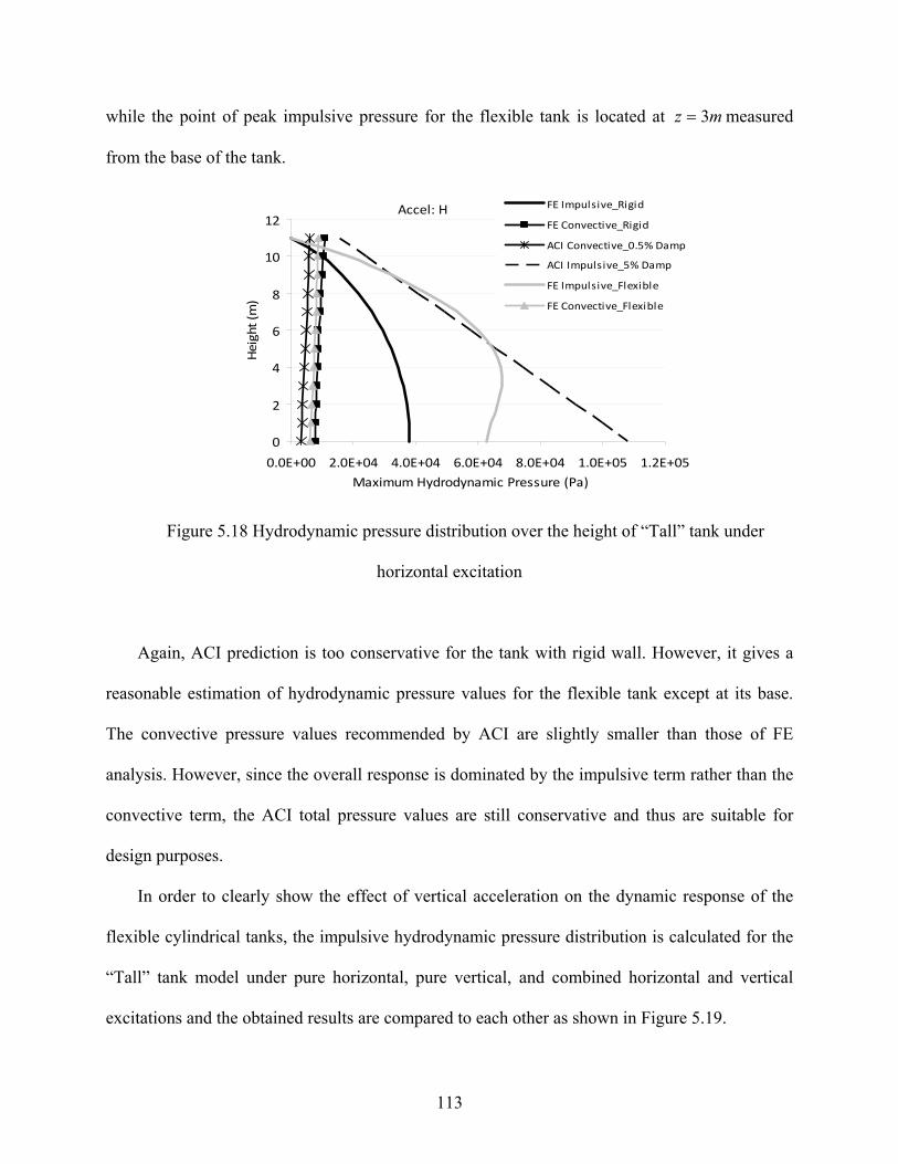
113

while the point of peak impulsive pressure for the flexible tank is located at mz 3 measured

from the base of the tank.

0

2

4

6

8

10

12

0.0E+00 2.0E+04 4.0E+04 6.0E+04 8.0E+04 1.0E+05 1.2E+05


Height (m

)

FE Impulsive_Rigid

FE Convective_Rigid



FE Impulsive_Flexible

FE Convective_Flexible

Accel: H

Figure 5.18 Hydrodynamic pressure distribution over the height of “Tall” tank under


Again, ACI prediction is too conservative for the tank with rigid wall. However, it gives a

reasonable estimation of hydrodynamic pressure values for the flexible tank except at its base.

The convective pressure values recommended by ACI are slightly smaller than those of FE

analysis. However, since the overall response is dominated by the impulsive term rather than the

convective term, the ACI total pressure values are still conservative and thus are suitable for

design purposes.

In order to clearly show the effect of vertical acceleration on the dynamic response of the

flexible cylindrical tanks, the impulsive hydrodynamic pressure distribution is calculated for the

“Tall” tank model under pure horizontal, pure vertical, and combined horizontal and vertical

excitations and the obtained results are compared to each other as shown in Figure 5.19.

114

0

2

4

6

8

10

12

0.0E+00 2.0E+04 4.0E+04 6.0E+04 8.0E+04 1.0E+05 1.2E+05Maximum Hydrodynamic Pressure (Pa)

Height (m

)

H

V

H+V

Figure 5.19 Impulsive pressure distribution along the height of the flexible “Tall” tank

It can be observed from the figure that the effect of vertical ground motion could be as high

as that of the horizontal motion when considered separately, however this effect is of less

significance when horizontal and vertical earthquake components are considered to be applied

simultaneously to the structure. Similar trend is also observed in “Shallow” tank model.

The results obtained for “Shallow” and “Tall” tanks also show that very small convective

response values are resulted due to pure vertical excitations. This has also been concluded by

Haroun and Tayel (1985) who stated that little or no sloshing occurs due to transient vertical

motions. Therefore, in obtaining the seismic response of cylindrical tanks to pure vertical

random excitations, the effect of convective fluid motion (sloshing) can be neglected and as a

result it can be assumed that the overall response of the tank-liquid system is fully dominated by

the impulsive term.

115

5.6 Effect of base fixity

To investigate the effect of base fixity on the dynamic behavior of cylindrical tanks, models

having different base conditions; fixed and hinged are subjected to both horizontal and vertical

seismic excitations and their dynamic response is calculated. Analyses are performed on both

“Shallow” and “Tall” tank models.

Figure 5.20 shows the envelope diagrams of hoop force, bending moment, and shear force

along the height of the flexible “Shallow” tank due to horizontal excitation.

Comparing the structural response values given in Figure 5.20 for hinged and fixed tank

models, it can be concluded that in general, higher maximum response values are found for tanks

having hinged base compared to those having fixed base especially near the mid-height of the

wall. However, this is not the case at the base. The maximum absolute values of the base shear

and the base moment for the fixed tank are higher than those of the hinged tank. It should be

noted that the value of moment at the base of the hinged tank and also hoop force value at the

base of tanks having either fixed or hinged conditions is zero.

Under pure vertical and also the combined effect of horizontal and vertical excitations, the

same trend as that presented here for pure horizontal excitation is observed. “Tall” tank model

also shows a similar trend as “Shallow” tank as described here. For the sake of brevity, those

results are not presented here.

116

0

1

2

3

4

5

6

0.0E+00 2.0E+05 4.0E+05 6.0E+05 8.0E+05

Maximum Hoop Force (N/m)

Height (m

)

Hinged

Fixed

Accel: H

(a)

0

1

2

3

4

5

6

‐6.0E+04 ‐4.0E+04 ‐2.0E+04 0.0E+00 2.0E+04 4.0E+04

Maximum Moment (N.m/m)

Height (m

)

Hinged

Fixed

Accel: H

(b)

0

1

2

3

4

5

6

‐6.0E+04 ‐4.0E+04 ‐2.0E+04 0.0E+00 2.0E+04 4.0E+04 6.0E+04

Maximum Shear (N/m)

Height (m

)

Hinged

Fixed

Accel: H

(c)

Figure 5.20 Envelope diagrams for flexible “Shallow” tank model due to horizontal

excitation; (a) Hoop force, (b) Moment, (c) Shear force

Figure 5.21 indicates the hydrodynamic pressure distribution over the height of flexible

“Shallow” tank due to horizontal excitation for tanks having fixed and hinged base connections.

The corresponding pressure distribution for flexible “Tall” tank model under horizontal

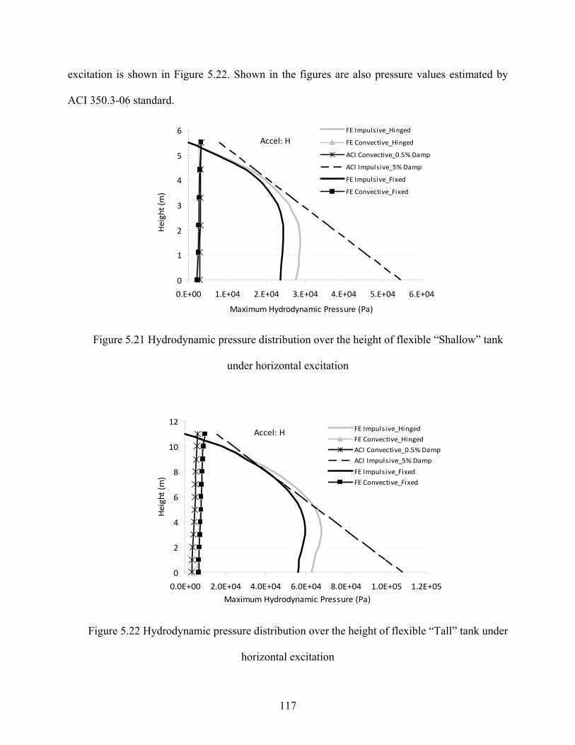
117

excitation is shown in Figure 5.22. Shown in the figures are also pressure values estimated by

ACI 350.3-06 standard.

0

1

2

3

4

5

6

0.E+00 1.E+04 2.E+04 3.E+04 4.E+04 5.E+04 6.E+04


Height (m

)

FE Impulsive_Hinged

FE Convective_Hinged



FE Impulsive_Fixed

FE Convective_Fixed

Accel: H

Figure 5.21 Hydrodynamic pressure distribution over the height of flexible “Shallow” tank

under horizontal excitation

0

2

4

6

8

10

12

0.0E+00 2.0E+04 4.0E+04 6.0E+04 8.0E+04 1.0E+05 1.2E+05


Height (m

)

FE Impulsive_Hinged

FE Convective_Hinged



FE Impulsive_Fixed

FE Convective_Fixed

Accel: H

Figure 5.22 Hydrodynamic pressure distribution over the height of flexible “Tall” tank under


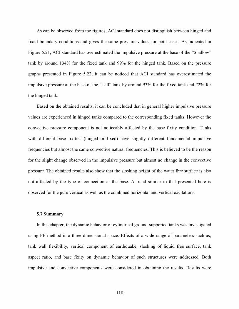
118

As can be observed from the figures, ACI standard does not distinguish between hinged and

fixed boundary conditions and gives the same pressure values for both cases. As indicated in

Figure 5.21, ACI standard has overestimated the impulsive pressure at the base of the “Shallow”

tank by around 134% for the fixed tank and 99% for the hinged tank. Based on the pressure

graphs presented in Figure 5.22, it can be noticed that ACI standard has overestimated the

impulsive pressure at the base of the “Tall” tank by around 93% for the fixed tank and 72% for

the hinged tank.

Based on the obtained results, it can be concluded that in general higher impulsive pressure

values are experienced in hinged tanks compared to the corresponding fixed tanks. However the

convective pressure component is not noticeably affected by the base fixity condition. Tanks

with different base fixities (hinged or fixed) have slightly different fundamental impulsive

frequencies but almost the same convective natural frequencies. This is believed to be the reason

for the slight change observed in the impulsive pressure but almost no change in the convective

pressure. The obtained results also show that the sloshing height of the water free surface is also

not affected by the type of connection at the base. A trend similar to that presented here is

observed for the pure vertical as well as the combined horizontal and vertical excitations.

5.7 Summary

In this chapter, the dynamic behavior of cylindrical ground-supported tanks was investigated

using FE method in a three dimensional space. Effects of a wide range of parameters such as;

tank wall flexibility, vertical component of earthquake, sloshing of liquid free surface, tank

aspect ratio, and base fixity on dynamic behavior of such structures were addressed. Both

impulsive and convective components were considered in obtaining the results. Results were

119

calculated for two different aspect ratios, representative of shallow and tall tanks in order to

investigate the effect of geometry on the dynamic response of the cylindrical containers. The

tanks were assumed to be rigidly anchored to the rigid ground. In order to evaluate the accuracy

of current practice, the obtained finite element results were compared with those recommended

by the ACI 350.3-06 standard.

The validity of the proposed FE method in both free vibration and time history analyses of

cylindrical containers was verified by comparing the calculated FE results with those obtained

through analytical approaches available in the literature.

In the first part of the chapter, free vibration analysis was carried out on the rigid tank

models. Effect of higher sloshing and impulsive modes and their associated effective mass ratios

and mode shapes were investigated. The obtained results including the natural frequencies, and

effective modal mass ratios compared very well with those calculated through analytical

procedures introduced by Housner (1963) and Veletsos and Shivakumar (1997). It was observed

that for practical purposes, only the fundamental impulsive and convective modes are sufficient

for characterizing the dynamic response of such tanks to horizontal excitations.

The results also revealed that the cos(nθ) type modes (n > 1) had a very small effect on the

overall dynamic response of the tanks to horizontal excitations. Modes having the highest

contributions to the response were cantilever beam type modes with n = 1.

In the second part of the chapter, time history analysis was performed on both rigid and

flexible tanks having different types of connection at the base; fixed and hinged under both

horizontal and vertical components of earthquake using the direct integration method.

Appropriate damping ratios corresponding to water components were selected according to ACI

350.3-06. Making use of the proposed finite element method, studying the contribution of both

120

impulsive and convective components of response was made possible. The examined responses

were sloshing height, hydrodynamic pressure and the associated structural forces including hoop

force, moment, and shear force. The obtained FE results were also compared with those

suggested by ACI 350.3-06 standard.

It was shown that the resulting convective forces have less effect on the overall dynamic

response of the tanks as compared to the impulsive forces. As a result, the seismic behavior of

the tanks was mainly dominated by the impulsive component rather than the convective

component.

It was clearly seen that since the sloshing and impulsive components of the response did not

reach their peak values at the same time, the effect of considering convective term on the total

response might be either increasing or decreasing.

It was also observed that the effect of convective term on the overall dynamic response of

liquid containers was rather more significant in shallow tanks compared to tall tanks.

Comparing the results obtained for rigid and flexible tanks revealed that including the wall

flexibility resulted in a significant increase on the impulsive part of response and therefore, this

effect should be taken into consideration in seismic design of the tanks. However, the convective

part of response was found to be almost independent of the tank wall flexibility and instead, it

seemed to be dependent on tank’s geometrical properties, fluid properties, and ground motion

characteristics. Furthermore, it was indicated that the sloshing height of the liquid inside the

tanks was not significantly affected by the wall flexibility.

Considering the combined effect of horizontal and vertical excitations, it was shown that

including the vertical acceleration effect led to an increase in both impulsive and convective

terms of response for “Shallow” as well as “Tall” tank models. It was also observed that the

121

vertical ground acceleration had a greater effect on the convective component of response than it

had on the impulsive component. The overall effect of vertical acceleration was found to be

insignificant in “Shallow” tank model. The sloshing height also increased as a result of combined

effect of vertical ground motion. It was found that the vertical acceleration had a relatively

greater effect on the response of “Tall” tank as compared to the “Shallow” tank. Therefore, the

effect of vertical ground motion needs to be taken into consideration appropriately in seismic

analysis of tall cylindrical containers and it should not be ignored.

The obtained results also show that the pure vertical ground motion could cause dynamic

effects as high as those of the horizontal motion when considered separately, however its effect

is found to be of less importance when horizontal and vertical earthquake components are

applied together.

It was also concluded that pure vertical transient excitations result in very negligible

convective response values for both tank configurations considered. As a result, one can ignore

the effect of convective component in determining the seismic response of cylindrical tanks

under pure vertical transient motions.

It was indicated that ACI 350.3-06 standard does not appropriately account for the effects of

wall flexibility and base fixity. That is, it gives the same hydrodynamic pressure values for rigid

and flexible tanks as well as for hinged and fixed tanks. As a result, ACI estimations could be too

conservative for the case of rigid tanks. This point needs further consideration in current liquid

tank design codes and standards.

Based on the obtained results, one can conclude that in general Code provisions yield a

conservative estimation of results, especially for the case of rigid tanks. This was observed for

“Shallow” as well as “Tall” tanks. In addition, since the hydrodynamic pressure approximated by

122

the Code has a linear vertical distribution, the Code estimations of hydrodynamic pressure could

be too conservative for the sections near the base.

Studying the dynamic behavior of tanks with different base fixity conditions revealed that

generally larger structural response values were developed in the walls of a hinged tank as

compared to a fixed tank far from the base. However, the maximum absolute values of the base

shear and the base moment were higher in the case of a fixed tank compared to a hinged one. It

was also shown that larger impulsive pressure values were exerted on the walls of a hinged tank

compared to an analogous fixed tank. However, the base fixity condition had no significant

effect on the convective pressure component. Sloshing height was also found to be insensitive to

the type of connection at the base.

Results of this study show that the proposed FE procedure can be accurately employed in the

transient analysis of cylindrical ground-supported tanks. Using this method, one can account for

all aspects in fluid-structure interaction problems including wall flexibility, sloshing motion,

damping properties of fluid domain, and the individual effects of impulsive and convective terms

in a 3D space.

123

CHAPTER 6

DYNAMIC RESPONSE OF LIQUID-FILLED ELEVATED TANKS

6.1 Introduction

In this chapter, the dynamic behavior of conical elevated tanks is studied in a three

dimensional space. The finite element technique is used to investigate the seismic response of

liquid-filled elevated tanks supported on a concrete shaft. The accuracy of this method in

analysis of ground-supported cylindrical tanks having different aspect ratios was verified in the

previous chapter. This chapter is divided into two main parts.

The primary objective of the first part is to propose a finite element model in order to

evaluate the performance of liquid-filled elevated tanks under seismic loading. Moreover, the

adequacy of current code provisions in estimating the seismic response of elevated water tanks is

studied. To this end, both time history and modal analyses are performed on an elevated tank.

Using the proposed FE technique, impulsive and convective response components are obtained

separately. Furthermore, the effect of tank wall flexibility and sloshing of the water free surface

are accounted for in the FE analysis. The linear free surface boundary condition is used for

simulating the sloshing behavior of the contained liquid. In this part of the chapter, also

difficulties associated with modeling of the tanks having complex geometries such as conical

elevated tanks are discussed.

The main focus of the second part is to investigate the effect of earthquake frequency

content on the dynamic behavior of liquid-filled elevated tanks. To do so, a three-dimensional

partially filled elevated tank is numerically simulated using FEM and its seismic behavior is

analyzed under the effect of different ground motion excitations having different frequency

124

content characteristics. In order to investigate the effect of earthquake frequency content, four

different earthquake records including El-Centro, Northridge, San-Francisco, and San-Fernando

are used.

The FE method proposed in this study has some advantages compared to previous analytical

research studies done on elevated tanks. One of the main features of the current method is in

considering the effect of liquid damping properties and accounting for impulsive and convective

terms separately. This has not been addressed previously. As a result, desired damping

characteristics corresponding to the two components may be defined separately. In addition, the

response of both components can be determined individually.

Furthermore, because of the inclination of the walls in conical elevated tanks, different

boundary conditions from those acting on cylindrical tanks exist. For design purposes, usually

the whole vessel is modeled as an equivalent cylindrical tank and thus the conical part of the

vessel is ignored in modeling. However, using the rigorous technique presented in this study, one

can accurately model the effect of fluid-structure interaction in tanks having complex geometries

such as conical tanks. In this chapter, also practical instructions to conquer these simulation

complexities are addressed.

Through this study, important factors such as the effects of tank wall flexibility, rocking as

well as translational motions of the vessel, tank/pedestal interaction, and higher impulsive and

convective modes are taken into account in FE modeling of the tanks. The proposed method is

capable of accounting for all these effects simultaneously.

125

6.2 General dynamic behavior of conical elevated tanks

6.2.1 Validity study of current practice

In order to evaluate the validity of current practice in predicting the dynamic response of

liquid-filled elevated tanks, the dynamic response of an elevated tank model is determined using

both current practice and FE approaches. The obtained results are then compared to each other.

Based on the obtained results, important conclusions regarding both the validity of current

practice and the general dynamic behavior of such structures are drawn. The procedure employed

by current practice for estimating the seismic response of liquid-filled tanks is explained in the

next subsection.

6.2.1.1 Seismic design forces based on current practice

For design of elevated water tanks in North America, the ACI 350.3-06 standard in

conjunction with ASCE 7-05 are used. These two standards are referred to as “current practice”

in this chapter. According to current practice, the seismic base shear (V ) is computed from the

following equation:

R

IeCWV (6-1)

where, C is the period-dependant seismic response coefficient for impulsive ( iC ) or

convective ( cC ) term, and eW is the effective weight of the system corresponding to impulsive

or convective components which is adapted from Housner’s method (Housner 1963). I is the

importance factor and R is the response modification factor corresponding to impulsive or

convective term. The related formulations for seismic response coefficients and other important

information regarding the current practice procedure can be found in section 3.3 of the thesis.

126

Total base shear (V ) and base moment ( M ) of the structure are determined by taking the

square root of the sum of the squares (SRSS) of the impulsive and convective terms.

6.2.1.2 Finite element analysis

A liquid-filled elevated tank is modeled and FE analyses are conducted using 3D fluid

elements. The calculated results through free vibration analysis, including natural periods of

vibration and effective masses corresponding to each mode of vibration, are compared with those

obtained from Housner's method (Housner 1963).

The equation of motion of the system can be solved by the direct integration method.

However, since the response of the structure is assumed to be linear, the more efficient analysis

using the concept of modal superposition by only including the contribution of significant natural

modes is used.

The unidirectional horizontal seismic excitation is applied to the system and the

corresponding instantaneous values of shear and moment at the base of the shaft are calculated.

The study includes the coupling between the impulsive response of the liquid and the shell and

also the sloshing effects.

According to ACI 371R-08 for each model, a sufficient number of modes (both impulsive

and convective) to obtain a combined modal mass participation of at least 90% of the actual mass

of the structure in the direction under consideration are employed.

The natural periods and associated mode shapes of the structure are computed by solving the

eigenvalue problem (Chopra 2000). Using the concept of equivalent simple oscillators, the tank-

pedestal system in ith mode of vibration can be idealized with an equivalent single degree of

freedom oscillator having an equivalent mass ( im ), an equivalent height ( iH ), natural frequency

127

( i ), and damping ratio ( i ). Employing this technique, the equation of motion of the whole

system can be converted to “i” independent differential equations corresponding to “i” equivalent

single degree of freedom oscillators.

By equating the base shear and kinetic energy of the equivalent simple oscillator with those

of the tank-pedestal system, the value of im , known as the effective modal mass as described in

most references on structural dynamics can be obtained.

The equivalent height ( iH ) corresponding to each mode is computed as the ratio of base

moment reaction (My) obtained by integrating over the vertical reactions (Fz) multiplied by their

associated arms (measured from the axis of symmetry at the shaft base) to the base horizontal

reaction (Fx).

Having obtained the values of the equivalent mass ( im ) and the equivalent height ( iH )

corresponding to each mode, one can find the instantaneous base shear and base moment

contributed from ith mode as follows:

)()( ttiuimtiQ (6-2)

)()( ttiuiHimtiM (6-3)

where, )(ttiu is the total acceleration of the equivalent simple oscillator subjected to the

known ground acceleration ( )(0 tu ).

The maximum numerical value of )(ttiu may be obtained from the pseudo-acceleration

response spectrum for the prescribed seismic motion ( )(0 tu ) using the natural frequency ( i )

and the associated damping ratio ( i ) corresponding to the ith mode.

128

Finally, the total base shear and base moment of the tank-pedestal system can be computed

by simply adding the time history values of modal base shears and base moments obtained from

equations (6-2) and (6-3) for sufficient number of modes.

Using this technique, base shear and base moment values corresponding to impulsive and

convective components of response can be determined separately. The adequacy of current

practice in estimating the seismically induced forces in elevated water tanks can be examined by

comparing the results from FEM explained here with those provided by the Code.

6.2.2 Numerical model verification

To further verify the current FE technique, the free vibration response of a small-scale

aluminum conical tank is obtained using the current FE technique and the results are compared

with the experimental values obtained by El Damatty et al. (2005).

In his study, El Damatty has conducted shake table testing as well as numerical analysis to

determine the dynamic properties of a conical tank specimen. The geometry and corresponding

finite element model used in the current study is indicated in Figure 6.1. Aluminum shell is

modeled as linear elastic material with the following properties:

Young's modulus = 69 GPa

Poisson's ratio = 0.33


Only displacement degrees of freedom are restrained for nodes located at the base. As a

result, the rotations are free to happen at the base nodes. The natural frequencies and effective

masses corresponding to both sloshing and liquid-shell vibration modes are obtained using

current FE technique and the results are summarized in Table 6.1.

129

(a) (b)

Figure 6.1 Geometry of the conical tank model;

(a) Side view, adapted from El Damatty et al. (2005),

(b) Finite Element model used in current study

Table 6.1 Free vibration analysis results for the conical tank model

Mode type El Damatty et al. (2005) Current study

Frequency (Hz) Ri (%) Frequency (Hz) Ri (%)

Fundamental convective 0.82 58.0 0.84 56.6

First liquid-shell mode 15.60 Negligible

15.11 Negligible

Second liquid-shell mode 18.40 17.97

First cosθ mode 43.50 40.7 42.36 41.5

In the table, Ri is defined as the ratio of the effective modal mass in the direction under

consideration to the total mass of the water. As shown in Table 6.1 the obtained FE results are in

excellent agreement with experimental results verifying that the current method can be employed

with high accuracy to study the fluid-structure interaction problems of conical liquid containers.

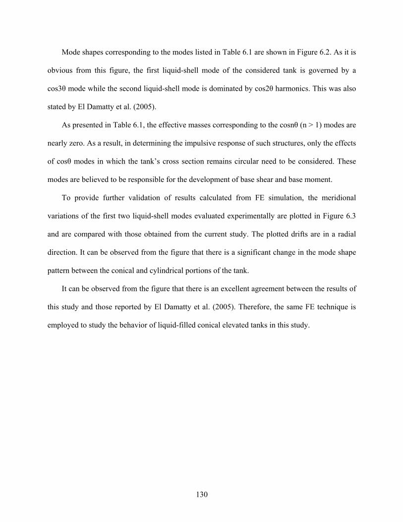
130

Mode shapes corresponding to the modes listed in Table 6.1 are shown in Figure 6.2. As it is

obvious from this figure, the first liquid-shell mode of the considered tank is governed by a

cos3θ mode while the second liquid-shell mode is dominated by cos2θ harmonics. This was also

stated by El Damatty et al. (2005).

As presented in Table 6.1, the effective masses corresponding to the cosnθ (n > 1) modes are

nearly zero. As a result, in determining the impulsive response of such structures, only the effects

of cosθ modes in which the tank’s cross section remains circular need to be considered. These

modes are believed to be responsible for the development of base shear and base moment.

To provide further validation of results calculated from FE simulation, the meridional

variations of the first two liquid-shell modes evaluated experimentally are plotted in Figure 6.3

and are compared with those obtained from the current study. The plotted drifts are in a radial

direction. It can be observed from the figure that there is a significant change in the mode shape

pattern between the conical and cylindrical portions of the tank.

It can be observed from the figure that there is an excellent agreement between the results of

this study and those reported by El Damatty et al. (2005). Therefore, the same FE technique is

employed to study the behavior of liquid-filled conical elevated tanks in this study.

131

Fundamental convective mode: (a) 3D view, (b) side view

First liquid-shell mode: (c) 3D view, (d) plan view

Second liquid-shell mode: (e) 3D view, (f) plan view

First cosθ mode - side view

Figure 6.2 Conical tank mode shapes

(a) (b)

(c) (d)

(e) (f)

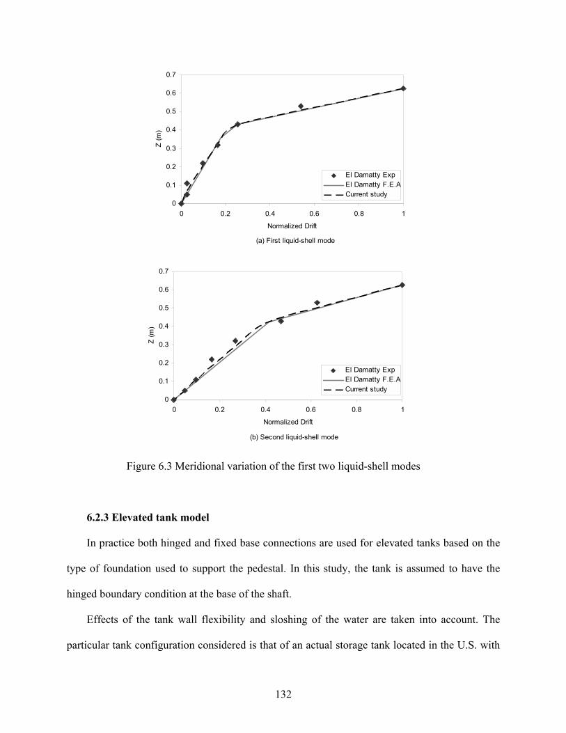
132

(a) First liquid-shell mode

0

0.1

0.2

0.3

0.4

0.5

0.6

0.7

0 0.2 0.4 0.6 0.8 1

Normalized Drift

Z (

m)

El Damatty ExpEl Damatty F.E.ACurrent study

(b) Second liquid-shell mode

0

0.1

0.2

0.3

0.4

0.5

0.6

0.7

0 0.2 0.4 0.6 0.8 1

Normalized Drift

Z (

m)

El Damatty ExpEl Damatty F.E.ACurrent study

Figure 6.3 Meridional variation of the first two liquid-shell modes

6.2.3 Elevated tank model

In practice both hinged and fixed base connections are used for elevated tanks based on the

type of foundation used to support the pedestal. In this study, the tank is assumed to have the

hinged boundary condition at the base of the shaft.

Effects of the tank wall flexibility and sloshing of the water are taken into account. The

particular tank configuration considered is that of an actual storage tank located in the U.S. with

133

the full capacity of 7571 m3 (2 MG). The simplified geometry of the tank is indicated in Figure

6.4. As shown in the figure, the actual tank’s floor is a concrete dome. However, because of

element shape irregularities occurring during mesh generation of fluid domain located inside the

conical portion of the vessel, the floor is modeled as a flat shell.

The effects of such simplification were investigated in this study and it was found to have

little effect on the total response. The fundamental mode shapes (both impulsive and convective)

of the tank are not generally influenced by the shape of the tank’s floor. The properties of the

fundamental impulsive mode are mainly dependent on the geometry and stiffness properties of

the supporting shaft. In comparison, the fundamental convective mode is mainly affected by the

geometry (aspect ratio) of the top cylinder and to a lesser extent by the geometry of the conical

portion of the vessel. As a result, such an assumption could only result in a slight increase in the

height of the contained water and as a result a slight reduction in the convective mass ratio

(L

CW

W ). Furthermore, since the total response is mainly dominated by the impulsive

component, the effect of such an assumption on the total response of the model will be

negligible.

Other geometric properties not given in Figure 6.4 are as follows:

side shell thickness: 8.8 mm

cone thickness: 24.5 mm

tank floor thickness: 330 mm

shaft thickness: 380 mm

134

Figure 6.4 Elevated tank geometry

The equivalent weight of platforms inside the shaft with their full live load is accounted for

by adding a distributed mass (total mass 715×103 kg) applied at 15.6 m above the base.

Moreover, a mass balance of 438 ×103 kg corresponding to the weight of the components (e.g.

roof, access tube, etc.) is applied around the ring beam as a distributed mass.

The density of water used is 1000 kg/m3. Concrete and steel elements are modeled as linear

elastic material. The following material properties are assumed for the steel and concrete shells:

Steel material:

Young's modulus= 200 GPa

Poisson's ratio= 0.30

Density= 7898 kg/m3

Concrete material:

Young's modulus= 24.86 GPa


Density= 2400 kg/m3

A total of 16464 fluid elements along with 2996 shell elements are used for modeling the

tank. In meshing fluid and shell domains, the nodes of fluid elements located on the interface

135

must be coincident with those of the surrounding shell elements. Then, coupling should be

defined between these coincident nodes such that equal displacements could occur in the radial

direction. There is no need to define coupling in any other direction. Therefore, tangential

relative displacements should be allowed to happen.

Coupling should be defined between the coincident nodes of fluid and structural domains at

all interfaces. Therefore, nodes of fluid domain located at the interface with the tank’s floor

should also be coupled with those of floor elements.

To couple the nodes located at the conical portion of the vessel, first the radial coordinates

(in the cylindrical coordinate system) of the fluid-shell nodes located along the cone interface

should be rotated by the cone angle ensuring that all nodes are aligned perpendicular to the cone

shell. Then, the rotated nodes can be coupled in the direction normal to the surface.

The conical section of the vessel has one interface with the cylindrical side shell at the top

and one with the concrete floor at the bottom. In order to define the liquid domain boundary

condition correctly, shell nodes located along these two boundary lines should be coupled to the

corresponding fluid nodes in two orthogonal directions. This is performed by introducing a new

coordinate system at these locations.

In the finite element idealization, the fluid domain is modeled using eight-node brick fluid

elements as described previously and the tank’s wall is modeled using four-node quadrilateral

shell elements. The element has six degrees of freedom (translations and rotations) at each node

and both bending and membrane behaviors are permitted. The finite element configuration of the

elevated tank model is indicated in Figure 6.5.

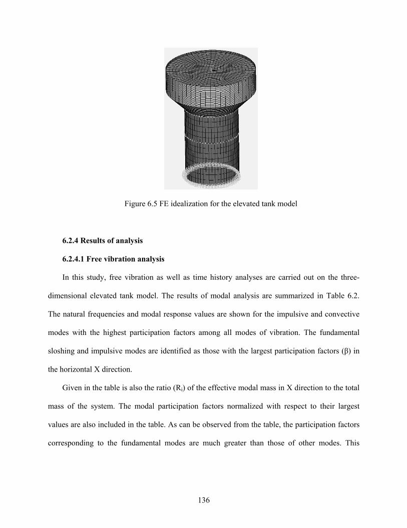
136

Figure 6.5 FE idealization for the elevated tank model

6.2.4 Results of analysis

6.2.4.1 Free vibration analysis

In this study, free vibration as well as time history analyses are carried out on the three-

dimensional elevated tank model. The results of modal analysis are summarized in Table 6.2.

The natural frequencies and modal response values are shown for the impulsive and convective

modes with the highest participation factors among all modes of vibration. The fundamental

sloshing and impulsive modes are identified as those with the largest participation factors (β) in

the horizontal X direction.

Given in the table is also the ratio (Ri) of the effective modal mass in X direction to the total

mass of the system. The modal participation factors normalized with respect to their largest

values are also included in the table. As can be observed from the table, the participation factors

corresponding to the fundamental modes are much greater than those of other modes. This

137

indicates that the response of the system is dominated by the fundamental modes under

horizontal excitations.

Included in the table are also water mass ratios and fundamental sloshing frequencies

obtained through Housner's method (Housner 1963) assuming vessels to be rigid. To use

Housner's formulae, the equivalent cylindrical model of the tank under consideration should be

determined. As recommended by some references available in the literature (ACI 371R-08

(2008), and Joshi (2000)), a close approximation for impulsive and convective masses of

axisymmetric tanks, other than cylindrical, may be obtained from an equivalent cylindrical tank

having the same free surface diameter and an equivalent water depth that results in an equal

volume of water for both the original and the equivalent tanks. Using the Housner’s formula

(Housner 1963), the convective and impulsive mass ratios of 56% and 40.4 % are obtained,

respectively.

Table 6.2 Free vibration analysis results for the elevated tank model

Mode Frequency(Hz) Effective mass × 103 kg (FE)

∑Ri (%) β (normalized) Number type FE Code FE Code

*1

Con

vect

ive 0.161

0.160 4302.51

58.7 56

1.00

2 0.161 235.38 0.23

3 0.294 NA 141.63 0.18

1

Impu

lsiv

e

1.955 2.980

918.36

41.3 40.4

0.46

*2 1.955 3367.52 0.88

3 7.470

NA

228.14 0.23

4 7.470 561.35 0.36

5 8.560 308.23 0.15

* Fundamental mode

138

In the Housner's method, the shell is assumed to be massless and only the mass of water is

considered in derivation of equations. Therefore, in order for the finite element results to be

comparable with those obtained from the Code (which is based on the Housner’s formula), only

the water mass contribution is considered in computing Ri, which is listed under the "FE"

column.

However, in determining the effective masses listed in the table, the contribution of both

fluid and shell element masses are taken into account. Since no shell deflection is observed

during the sloshing modes vibration, the entire effective mass obtained from FE contributes from

the sloshing liquid and not the non-moving shell. As a result, the convective mass ratio defined

as %7.58

L

Ci W

WR is obtained, where CW is the summation of the modal effective

masses corresponding to all sloshing modes and LW is the total equivalent weight of the stored

water. The rest of the liquid mass, i.e. 41.3%, behaves under impulsive modes.

Modes with exactly similar natural frequencies represent the same mode in two orthogonal

directions (X and Y). Each of these modes is deviated from X or Y axis by a small angle. The

effective masses are given as their projections on X axis.

As shown, the finite element results are in reasonable agreement with those calculated from

the Code using the concept of equivalent cylinder model, especially in terms of computed natural

frequencies. The difference in the convective mass values is less than 3 percent of the total mass

of the fluid. This difference is even smaller for the impulsive masses (less than 1 percent). These

findings are in agreement with those reported by Joshi (2000) who stated that for conical (Intze)

tanks with the equivalent depth to radius ratios between 0.5 and 1.0 (which is the case here), the

maximum errors for the impulsive and convective masses are less than around 5 and 6 percent of

139

the total liquid mass, respectively. The equivalent depth to radius ratio for the model considered

in this study is 0.71.

From the results given in Table 6.2, one can conclude that both impulsive and sloshing

behaviors of the considered model are practically dominated by its fundamental modes.

The modes given in Table 6.2 include about 93% of the total mass of the system. This

accumulated effective mass ratio is more than the minimum criterion recommended by current

practice.

As mentioned before, modes having the same natural frequencies are similar modes but in

two orthogonal directions. As a result, the mode shapes and other modal properties remain the

same for the first two convective and the first two impulsive modes.

All three sloshing modes given in Table 6.2 are associated with vertical water surface

displacements which are antisymmetric about the axis of rotation and change in the

circumferential direction as a cosine function. No shell vibration is observed during the

animation of these sloshing modes. This is in accordance with the well-known assumption of

decoupling the sloshing and the shell motions in liquid-containing structures.

All the impulsive modes presented in Table 6.2 are translational modes. These modes can be

classified as the cosθ-type modes during which the tank’s cross-section remains circular. During

the first two impulsive modes, the entire tank behaves like a vertical beam.

For higher impulsive modes (modes 3 to 5), the top cylinder of the vessel experiences more

pronounced deformation compared to the conical portion. This is partly due to the higher

stiffness attributes associated with the conical part compared to the cylindrical part which is in

turn because of the thicker shell assigned to the conical part as well as the geometric stiffening

effect. The other important factor is that a larger fluid mass per unit height is located at the top

140

portion of the tank compared to the conical section. The top cylinder can be considered as a

broad tank with the aspect ratio of H/D = 0.25. Therefore, as is the case for shallow tanks, their

mode shape is characterized by a bulge near the mid-height of the cylinder. This is observed in

the top cylinder for all higher impulsive mode shapes (modes 3 to 5).

Furthermore, the obtained mode shapes show a drastic change in the mode shape pattern

between the conical and the cylindrical portions of the tank in modes 3 to 5. As explained

before, this is due to a sudden change in stiffness and geometry at the cone/cylinder interface.

This abrupt change results in high localized deformations along the cone/cylinder interface.

For illustration purposes, the convective and impulsive mode shapes are shown in Figures

6.6 and 6.7, respectively. In the next section, the seismic behavior of the elevated tank model is

further investigated by performing time history analysis on the model.

141

(a) side view

(b) 3D view

Fundamental convective mode (Mode 1)

Higher convective mode (Mode 3)

Figure 6.6. Elevated tank mode shapes (convective modes)

142

(a) side view

(b) 3D view

Fundamental impulsive mode (Mode 2)

Higher impulsive mode (Mode 4)

Higher impulsive mode (Mode 5)

Figure 6.7. Elevated tank mode shapes (impulsive modes)

143

6.2.4.2 Time history analysis

The horizontal component of 1940 El-Centro ground motion with the peak ground

acceleration of 0.32g as shown in Figure 6.8 is used for time history analysis. Earthquake

duration is around 31 seconds with its peak value occurring at 2.02 second. Since the sloshing

component of motion continues long after the earthquake ceases and moreover, the maximum

sloshing response generally occurs at a later time than that of impulsive response, the ground

motion is continued beyond the duration of earthquake and for up to 60 seconds at zero

acceleration allowing for the sloshing response to be fully developed.

An integration time step of 0.005 second is used to be small enough to characterize the

response. Damping is assigned as a constant damping ratio to each mode considered for modal

superposition analysis separately. The damping ratios of 5 and 0.5 percent are used for impulsive

and sloshing modes, respectively.

As explained before, a sufficient number of modes are used so that the ratio of the

accumulated effective mass to the total mass of the system (∑Ri ) reaches at least 90%.

Consequently, a total of eight modes (three convective and five impulsive modes) as presented in

Table 6.2 are used for time history analysis of the elevated tank model.

For quantitative comparison of the seismic response of the considered model under random

ground excitation, the time history values of base shear (V) and base moment (M) of the model

subjected to El-Centro earthquake are obtained using the modal superposition technique. The

modes listed in Table 6.2 are used to carry out such an analysis.

Time history results have been separated into the impulsive and convective components.

Therefore, the maximum response values associated with each component (impulsive or

convective) and the instants at which these maxima occur may be determined separately.

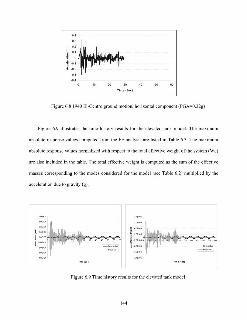
144

-0.4

-0.3

-0.2

-0.1

0

0.1

0.2

0.3

0.4

0 10 20 30 40 50 60

Time (Sec)

Acc

eler

atio

n (

g)

Figure 6.8 1940 El-Centro ground motion, horizontal component (PGA=0.32g)

Figure 6.9 illustrates the time history results for the elevated tank model. The maximum

absolute response values computed from the FE analysis are listed in Table 6.3. The maximum

absolute response values normalized with respect to the total effective weight of the system (We)

are also included in the table. The total effective weight is computed as the sum of the effective

masses corresponding to the modes considered for the model (see Table 6.2) multiplied by the

acceleration due to gravity (g).

-4.0E+04

-3.0E+04

-2.0E+04

-1.0E+04

0.0E+00

1.0E+04

2.0E+04

3.0E+04

4.0E+04

0 5 10 15 20 25 30 35 40 45 50 55 60

Time (Sec)

Bas

e S

hea

r (K

N)

Convective

Impulsive

-1.4E+06

-1.0E+06

-6.0E+05

-2.0E+05

2.0E+05

6.0E+05

1.0E+06

1.4E+06

0 5 10 15 20 25 30 35 40 45 50 55 60

Time (Sec)

Bas

e M

om

ent

(KN

.M)

Convective

Impulsive

Figure 6.9 Time history results for the elevated tank model

145

Based on the data provided in Table 6.3, it can be concluded that the contribution of the

impulsive component in total seismic response of the elevated tank model is much higher than

that of the convective term. Contributions to the base shear and base moment of the shaft from

all sloshing modes are found to be negligible because of the very small response spectrum

accelerations associated with such low frequency modes. The maximum contribution of sloshing

component to the base shear of the shaft is only around 3 percent of the total effective weight of

the system while for the impulsive component this contribution could be as high as 36 percent.

Table 6.3 Maximum absolute time history response values for the elevated tank model

Convective Impulsive Total

Base shear

Max value (kN)

Ratio(%) (Vc/We)

Max value (kN)

Ratio(%) (Vi/We)

Max value (kN)

Ratio(%) (V/We)

2487 2.52 35548 36.03 34842 35.32

Base moment

Max value (kN.m)

Ratio (Mc/We)

Max value (kN.m)

Ratio (Mi/We)

Max value (kN.m)

Ratio (M/We)

94023 0.95 1320592 13.39 1293880 13.11

Table 6.3 also shows that adding the sloshing component of the response has resulted in a

reduction of forces. This is because of the fact that the water sloshing motion is not in phase with

the impulsive motion of the tank-pedestal system.

It is important to note that the peak of the sloshing response occurs far beyond that of the

impulsive response. For instance, the maximum impulsive response occurs at t = 2.34 s while the

sloshing response reaches its peak value at t = 29.97 s. As shown in Figure 6.9 when the peak

impulsive response occurs, the convective response is at the beginning stage and has not yet fully

developed.

146

At the end of the earthquake’s duration, the impulsive motion of the tank-pedestal system is

rapidly damped out, in contrast the sloshing part of the response continues at decreasing

amplitude for the remainder of the time period considered. This is because of the higher damping

ratio ( = 5%) associated with the impulsive component than that of the sloshing component

( = 0.5%).

6.2.5 Comparison of FE results with current practice

To evaluate the accuracy of the current practice in predicting the seismic response of

elevated water tanks, the base shear and base moment response values of the elevated tank model

are calculated according to the formulations given in section 6.2.1.1.

It should be noted that the response values obtained through current practice are based on

the values of I=1.5 and R=3 per ASCE 7-05, where I is the “Importance factor” and R is the

“Response modification coefficient”. Therefore, to compare these values with those obtained

from FE analysis, the calculated time history results (given in Table 6.3) are multiplied by I/R =

0.5.

In calculating the design forces using the current practice, the design spectrum with a peak

ground acceleration of 0.32g to correspond with the seismic ground motion used in FE analyses

is used. Moreover, the mapped spectral accelerations ( SS and 1S ) for Imperial Valley location

are chosen as 1.5g and o.6g, respectively. Site class "A", classified as a site with hard rock soil is

assumed for the Code analysis.

In obtaining the results using the current practice, first dynamic properties of the model

(natural periods of vibration and associated modal masses corresponding to the impulsive and

147

convective modes) are determined using a two-mass idealization approach developed by

Housner (1963).

To use Housner’s method, initially the conical (Intze) tank under consideration should be

converted to an equivalent cylindrical tank having the same volume of water as the original tank.

Then, the equivalent lumped masses and the equivalent heights of the impulsive and convective

components of the liquid inside the cylinder are calculated using Housner's formulae. In

obtaining the effective heights, the effect of hydrodynamic pressure exerted on the bottom of the

tank is included.

As shown in Figure 6.10(a), the actual elevated tank model consists of the following mass

components; convective mass of water ( CM ); equivalent mass twM which in turn includes the

impulsive mass of water and the walls of the vessel; mass of the tank’s floor ( drM ), and mass of

the shaft and interior platforms ( sM ). In order to simplify the calculation process, the actual tank

model is equated with a two degree of freedom model shown in Figure 6.10(b).

As shown in this figure, the entire mass of the tank-pedestal system is divided into

convective ( CM ) and impulsive ( IM ) components. The convective mass of the contained liquid

( CM ) and its location can be readily calculated based on Housner's method. It is assumed to be

connected to the walls of the vessel by a spring having the equivalent stiffness of 1K .

IM represents the impulsive mass of the system and is lumped at distance "a" above the tip

of the shaft. It includes the mass components of impulsive water, walls of the vessel, tank floor

( drM ), as well as shaft and its interior platforms ( sM ).

To determine IM and its location, initially, the mass components associated with the

impulsive water, and the walls of the vessel are equated with the mass twM , located at an

equivalent distance "a" from the top of the shaft. Having obtained the weights of the impulsive

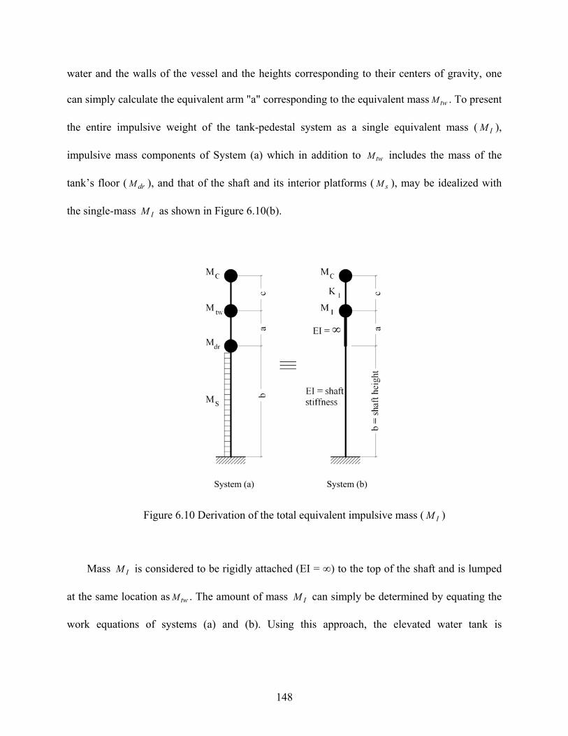
148

water and the walls of the vessel and the heights corresponding to their centers of gravity, one

can simply calculate the equivalent arm "a" corresponding to the equivalent mass twM . To present

the entire impulsive weight of the tank-pedestal system as a single equivalent mass ( IM ),

impulsive mass components of System (a) which in addition to twM includes the mass of the

tank’s floor ( drM ), and that of the shaft and its interior platforms ( sM ), may be idealized with

the single-mass IM as shown in Figure 6.10(b).

Figure 6.10 Derivation of the total equivalent impulsive mass ( IM )

Mass IM is considered to be rigidly attached (EI = ∞) to the top of the shaft and is lumped

at the same location as twM . The amount of mass IM can simply be determined by equating the

work equations of systems (a) and (b). Using this approach, the elevated water tank is

System (b) System (a)

149

represented as an equivalent two degree of freedom system as shown in Figure 6.11. Mechanical

parameters corresponding to this equivalent system are also shown in this figure.

The two modes of vibration with the natural periods of Tc= 6.250 sec and Ti= 0.336 sec are

identified for the equivalent two DOF system corresponding to convective and impulsive modes,

respectively.

(a) Actual model (b) Equivalent cylindrical model (c) Equivalent two DOF model

Figure 6.11 Elevated tank model and its equivalent dynamic system

The base shear and base moment corresponding to impulsive and convective components

can be obtained using equations described in section 6.2.1.1. The total base shear and base

moment can be calculated by combining the impulsive and convective terms using SRSS method

(see Table 6.4). The resulting base shear and base moment values are 16425 kN and 609557

kNm, respectively.

Comparing these results with those obtained from FE analysis, it can be concluded that

estimated responses are in reasonable agreement. The difference between two sets of data is only

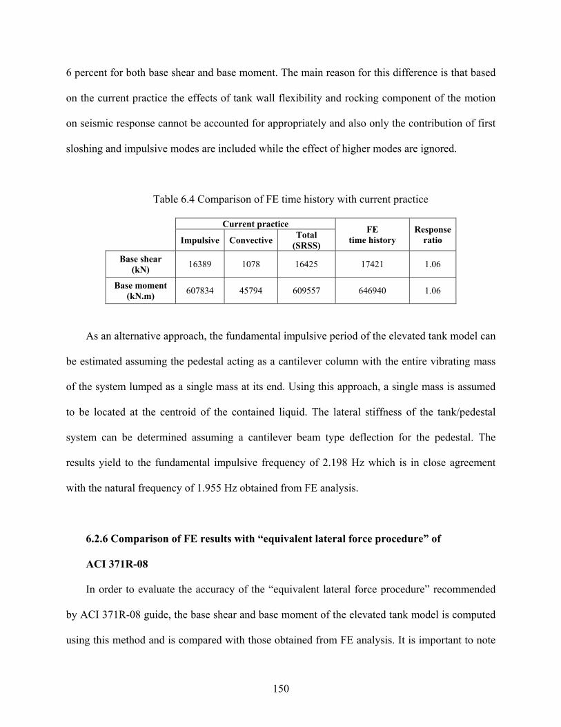
150

6 percent for both base shear and base moment. The main reason for this difference is that based

on the current practice the effects of tank wall flexibility and rocking component of the motion

on seismic response cannot be accounted for appropriately and also only the contribution of first

sloshing and impulsive modes are included while the effect of higher modes are ignored.

Table 6.4 Comparison of FE time history with current practice

Current practice

FE time history

Response ratio Impulsive Convective

Total (SRSS)

Base shear (kN) 16389 1078 16425 17421 1.06

Base moment (kN.m) 607834 45794 609557 646940 1.06

As an alternative approach, the fundamental impulsive period of the elevated tank model can

be estimated assuming the pedestal acting as a cantilever column with the entire vibrating mass

of the system lumped as a single mass at its end. Using this approach, a single mass is assumed

to be located at the centroid of the contained liquid. The lateral stiffness of the tank/pedestal

system can be determined assuming a cantilever beam type deflection for the pedestal. The

results yield to the fundamental impulsive frequency of 2.198 Hz which is in close agreement

with the natural frequency of 1.955 Hz obtained from FE analysis.

6.2.6 Comparison of FE results with “equivalent lateral force procedure” of

ACI 371R-08

In order to evaluate the accuracy of the “equivalent lateral force procedure” recommended

by ACI 371R-08 guide, the base shear and base moment of the elevated tank model is computed

using this method and is compared with those obtained from FE analysis. It is important to note

151

that in this approximate procedure, the sloshing behavior of the stored liquid is ignored and the

entire mass of water is considered as an impulsive mass.

According to “equivalent lateral force procedure”, the seismic base shear (V ) is determined

from:

eWCV s (6-4)

where, eW is the total effective weight of the system. sC is the seismic response coefficient

and is determined as follows:

R

ISC DSs (6-5)

sC should not be greater than

RT

ISC

fDs 1 (6-6)

but should not be taken less than

ISC DSs 044.0 (6-7)

where, I , R , DSS , and 1DS are as defined previously in sections 6.2.1.1 and 3.3 of the

thesis. fT is the fundamental period of the tank/pedestal system which is determined assuming

that the entire vibrating mass of the system is represented by a single lumped mass located at the

centroid of the contained water. Assuming the pedestal acting as a cantilever beam of length gL

having uniform stiffness with a single mass lumped at its end, fT can be determined as follows:

c

ef gk

WT 2 (6-8)

where, ck is the tank lateral stiffness which is determined as:

152

3

3

g

ccc

L

IEk (6-9)

in which, cE is the modulus of elasticity of concrete; cI is the moment of inertia of the gross

concrete section about the centroidal axis, neglecting reinforcement and gL is the distance from

base to centroid of the stored water. For a thin cylinder of thickness rh and mean diameter wd ,

the cross-sectional area cA and moment of inertia cI are calculated as:

rwc hdA (6-10)

23

)(125.0)(125.0 wcrwc dAhdI (6-11)

Substituting for cI , one can obtain the following approximate equation for fundamental

period fT :

gdEA

LWT

wcc

gef 2

3

3

82 (6-12)

As was mentioned previously, this assumption will lead to the fundamental frequency of

2.198 Hz. Once the seismic base shear is obtained, the lateral seismic force xF induced at any

level is determined by distributing the total lateral seismic force over the height of the structure

as follows:

VCF vxx (6-13)

n

iii

xxvx

hW

hWC

1

(6-14)

153

where, vxC is the vertical distribution factor, iW and xW are portion of the total effective

weight of the structure eW located or assigned to level i or x ; ih and xh are height from the

base to level i or x . The calculated lateral seismic forces xF for the elevated tank model under

consideration are shown in Figure 6.12. In calculating these lateral seismic forces, the design

spectrum as described previously in section 6.2.5 in conjunction with Eqs. (6-4) to (6-7) is used.

Figure 6.12 Lateral seismic forces obtained from “equivalent lateral force procedure”

In Figure 6.12, c.g.0 to c.g.6 are centers of gravity for different portions of the tank-pedestal

system defined as follows:

154

c.g.0: Center of gravity for cylindrical steel shell

c.g.1: Center of gravity for conical steel shell

c.g.2: Center of gravity for tank’s floor + Ring beam + other accessories

c.g.3: Center of gravity for interior platforms

c.g.4: Center of gravity for concrete pedestal

c.g.5 and c.g.6: Centers of gravity for impulsive and convective water components

The lateral seismic shear xV and overturning moment xM acting at level x is determined

by:

x

iix FV

1

(6-15)

)(1

x

ixiix hhFM (6-16)

where, iF is the portion of the seismic base shear induced at level i and is from the top of

the structure to the level under consideration.

Eqs. (6-15) and (6-16) lead to the base shear and base moment values of 36,430 kN and

1,246,402 kN.m, respectively for the elevated tank model under consideration. These values are

greater than those obtained from FE by a factor of 2.09 and 1.93, respectively. As expected,

seismic response values are highly overestimated using the “equivalent lateral force procedure”

recommended by ACI 371R-08, leading to an overdesign of the shaft structure and supporting

foundation. As a result, this procedure does not seem to be appropriate for evaluating the seismic

response of liquid-filled elevated tanks.

155

6.2.7 Comparison of FE results with “combined Code/FE” method

The seismic base shear and overturning moment at the base of the elevated tank may also be

computed using the modal response values obtained from FE analysis in combination with

response spectrum in accordance with current practice as defined under section 6.2.1.1.

As a result, dynamic properties of the model including the equivalent weights of the

impulsive and convective modes, natural periods of vibration, and associated moment arm for

each considered mode are first determined from a fluid-structure interaction analysis performed

using the ANSYS computer program. Then, the seismic response coefficients corresponding to

each mode under consideration are determined using the current practice as explained before. Eq.

(6-1) can then be used to calculate the seismic base shear contributed by each mode. The

corresponding overturning moment for each mode can be simply evaluated by multiplying the

computed base shear by the moment arm obtained from FE modal analysis.

The total impulsive response is obtained by combining the response values corresponding to

impulsive modes using the SRSS method. The same combination method may be used to obtain

the total convective response. Finally, computed impulsive and convective terms are again

combined using SRSS method to obtain the total base shear and base moment of the structure.

This leads to the total base shear and base moment values of 13,611 kN and 484,880 kNm,

respectively.

Comparing the contributions of impulsive and convective components, one can observe that

the contribution of convective term in total response is much smaller than that of impulsive.

Comparing the results of combined method with those obtained from FE analysis, it can be

observed that the combined method underestimates the base shear by 21% and base moment by

25% which is not desirable for design applications.

156

Comparing the results obtained through current practice presented in section 6.2.5 with

those of combined method, it can be seen that following the provisions of current practice lead to

relatively higher response values (21% for base shear and 26% for base moment).

These higher response values obtained from current practice are resulted from higher

seismic coefficient ( iC ) associated with the fundamental impulsive mode. This is in fact due to

lower period corresponding to fundamental impulsive mode estimated using current practice

compared to that obtained through FE analysis.

6.3 Effect of earthquake frequency content on the dynamic behavior of liquid-filled

elevated tanks

In order to investigate the effect of earthquake frequency content on the dynamic behavior

of liquid-filled elevated tanks, the same elevated tank model is subjected to four different ground

motions with different frequency content properties and the time history response values are

obtained.

It should be noted that in the previous section the time history response of the model was

determined using the modal superposition technique, however in the current section the direct

integration method is used for obtaining the transient response of the model. Furthermore, since

the sloshing component was found to have a negligible effect on the overall seismic behavior of

the tank, only the impulsive part of response is considered in this section and the effect of

sloshing term is neglected. Studied responses are shear and overturning moment at the base of

the pedestal.

157

The longitudinal components of 1940 El-Centro, 1994 Northridge, 1971 San-Fernando, and

1957 San-Francisco earthquakes are used as horizontal excitations for the elevated tank model.

Only the first 15 seconds of the records are used in time history analyses.

The El-Centro record is scaled in such a way that its peak ground acceleration reaches 0.4g.

Other records are scaled in such a way to have the same value of Power index ( aP ) (Housner

1975) as that of the scaled El-Centro record. Various indices have been proposed so far to

characterize the intensity of earthquake motions including: peak ground acceleration, Arias

intensity (Arias 1970), Power index (Housner 1975), Spectrum intensity (Housner 1952), and so

on.

Among all these indices, it is well known that the Power index is one of the most

appropriate indices to be used for scaling of the earthquake motions and as a result the intensity

of motions can be satisfactorily characterized by this parameter. The earthquake motions are

usually characterized by parameters related primarily to the amplitude of the shaking, such as

peak ground acceleration however, research studies show that it is not a reliable measure by itself

(Housner 1975). The single peak on an accelerogram can not be considered as an accurate

representation of the earthquake record as a whole.

Housner (1975) proposed that a measure of seismic intensity could be defined by the

average rate of buildup of the total energy per unit mass input to the structure. Taking into

consideration that the integral of the squared ground acceleration is proportional to the total input

energy, he introduced the Power index as:

Dt

ta dtta

DD

DEP

0

0

2

)(1)(

(6-17)

where,

158

)(DE is the total energy input during time D

D is the “significant duration” of earthquake

0t is the time at the beginning of the strong shaking phase

)(ta is the base acceleration

In other words, the Power index can be considered as a measure of the rate at which energy

would be fed into the system. In Eq. (6-17), 0t and Dt 0 are the limits of the strong portion of

motion. Eq. (6-17) can be interpreted as the average value of the squared acceleration over the

significant duration interval D .

Arias intensity (Arias 1970) relates to the sum of the energies dissipated per unit of mass by

a population of damped oscillators of all natural frequencies ( 0 ):

dttag

AIrt

0

2

)(2

(6-18)

where, rt is the total duration of the ground motion and g is the acceleration due to gravity.

If the strong shaking is considered to start at the beginning of the record, i.e. 0t is zero, the

following relation may be derived:

)(2 rtE

gAI

(6-19)

As it is obvious from this equation, the Arias intensity is actually representative of the total

energy in the record.

The popular definition of significant duration of motion proposed by Trifunac and Brady

(1975) is adopted in this study where the significant duration is defined as the interval between

instants 5t and 95t at which 5% and 95% of the total integral in Eq. (6-18) is attained,

respectively:

159

595 ttD (6-20)

The concept of significant duration has the benefit of considering the properties of the whole

accelerogram and defining a continuous time interval during which the shaking may be

considered as strong.

Finally, the earthquake Power can be defined as:

95

5

2

595

)(1

t

ta dtta

ttP (6-21)

The scaled earthquake records are shown in Figure 6.13. The Arias intensity versus time

(known as Husid plot) is also indicated in Figure 6.14 for all the earthquake records considered.

As it is obvious from this figure, all curves have equal initial slopes over the time interval

D (significant duration), implying that all scaled records have the same level of Power.

-0.5

-0.3

-0.1

0.1

0.3

0.5

0 5 10 15

Time (sec)

Ac

ce

lera

tio

n (

g)

-0.5

-0.3

-0.1

0.1

0.3

0.5

0 5 10 15

Time (sec)

Acc

eler

atio

n (

g)

(a) (b)

-0.5

-0.3

-0.1

0.1

0.3

0.5

0 5 10 15

Time (sec)

Acc

eler

atio

n (

g)

-0.5

-0.3

-0.1

0.1

0.3

0.5

0 5 10 15

Time (sec)

Acc

eler

atio

n (

g)

(c) (d)

Figure 6.13 Scaled earthquake records (horizontal component); (a) El-Centro,

(b) Northridge, (c) San-Fernando, (d) San-Francisco

160

0

0.5

1

1.5

2

2.5

0 3 6 9 12 15

Time (sec)

Ari

as

Inte

ns

ity

(m

/se

c)

El-Centro

Northridge

San-Fernando

San-Francisco

Figure 6.14 Arias Intensity versus time (Husid plot) of the earthquake records

The characteristics of the scaled records are listed in Table 6.5. The predominant frequency

( pf ) of each record is also given in the table.

Table 6.5 Ground motions properties

Earthquake )(5 st )(95 st )(sD )( 42 smPa )(Hzf p PGV

PGA

El-Centro 1.63 13.25 11.62 1.13 2.000 0.88

Northridge 2.12 9.14 7.02 1.12 1.282 0.51

San-Fernando 1.75 10.08 8.33 1.12 4.160 1.11

San-Francisco 1.18 4.15 2.97 1.13 4.545 2.44

The predominant frequency is defined as the frequency corresponding to the highest peak in

a response spectrum. For instance, the Pseudo-acceleration (PSA) response spectra

corresponding to 5% of critical damping are calculated for Northridge and San-Francisco

records, as shown in Figure 6.15. From this figure, one can determine the predominant

frequencies of 1.282 Hz and 4.545 Hz for Northridge and San-Francisco ground motions,

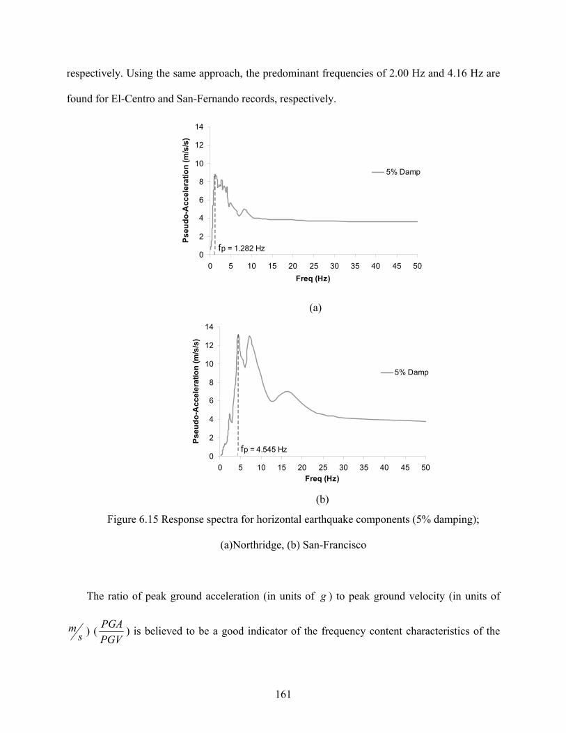
161

respectively. Using the same approach, the predominant frequencies of 2.00 Hz and 4.16 Hz are

found for El-Centro and San-Fernando records, respectively.

0

2

4

6

8

10

12

14

0 5 10 15 20 25 30 35 40 45 50

Freq (Hz)

Ps

eu

do

-Ac

ce

lera

tio

n (

m/s

/s)

5% Damp

fp = 1.282 Hz

(a)

0

2

4

6

8

10

12

14

0 5 10 15 20 25 30 35 40 45 50

Freq (Hz)

Ps

eu

do

-Ac

ce

lera

tio

n (

m/s

/s)

5% Damp

fp = 4.545 Hz

(b)

Figure 6.15 Response spectra for horizontal earthquake components (5% damping);

(a)Northridge, (b) San-Francisco

The ratio of peak ground acceleration (in units of g ) to peak ground velocity (in units of

sm ) (

PGV

PGA) is believed to be a good indicator of the frequency content characteristics of the

162

ground motion. As a result, ground motions with PGV

PGA<0.8 are classified as low frequency

content, earthquake records with 1.2>PGV

PGA>0.8 are classified as intermediate frequency

content, and those with PGV

PGA>1.2 can be classified as high frequency content. Therefore, the

Northridge record is categorized as low frequency content, the El-Centro and San-Fernando

records are categorized as intermediate frequency content and the San-Francisco record is

categorized as high frequency content.

The transient base shear and base moment for the elevated tank model due to horizontal

excitation are calculated using the proposed method. As mentioned before, four different seismic

excitations are applied to the model to investigate the effect of frequency content on the seismic

response of the tank-pedestal system. The time history base shear and base moment responses of

the tank subjected to these records are presented in Figures 6.16 and 6.17, respectively. It should

be noted that these values correspond with the total force and moment acting at the base of the

pedestal.

163

-6.0E+04

-4.0E+04

-2.0E+04

0.0E+00

2.0E+04

4.0E+04

6.0E+04

0 5 10 15

Time(s)

Ba

se S

he

ar (k

N)

-6.0E+04

-4.0E+04

-2.0E+04

0.0E+00

2.0E+04

4.0E+04

6.0E+04

0 5 10 15

Time(s)

Ba

se S

he

ar

(kN

)

(a) (b)

-6.0E+04

-4.0E+04

-2.0E+04

0.0E+00

2.0E+04

4.0E+04

6.0E+04

0 5 10 15

Time(s)

Ba

se S

he

ar

(kN

)

-6.0E+04

-4.0E+04

-2.0E+04

0.0E+00

2.0E+04

4.0E+04

6.0E+04

0 5 10 15

Time(s)

Ba

se

Sh

ear

(kN

)

(c) (d)

Figure 6.16 Time history of base shear response for the elevated tank model under



164

-2.00E+06

-1.20E+06

-4.00E+05

4.00E+05

1.20E+06

2.00E+06

0 5 10 15

Time(s)

Ba

se M

om

ent (

kN

m)

-2.00E+06

-1.20E+06

-4.00E+05

4.00E+05

1.20E+06

2.00E+06

0 5 10 15

Time(s)

Ba

se

Mo

me

nt

(kN

m)

(a) (b)

-2.00E+06

-1.20E+06

-4.00E+05

4.00E+05

1.20E+06

2.00E+06

0 5 10 15

Time(s)

Ba

se

Mo

me

nt

(kN

m)

-2.00E+06

-1.20E+06

-4.00E+05

4.00E+05

1.20E+06

2.00E+06

0 5 10 15

Time(s)

Ba

se M

om

en

t (k

Nm

)

(c) (d)

Figure 6.17 Time history of base moment response for the elevated tank model under



For comparison purposes, the peak FE results for various ground motions are normalized

with respect to the peak response values corresponding to the record producing the highest

response among four records considered. The variation of the dynamic response in terms of the

normalized peak base shear and base moment for different earthquake records is shown in Figure

6.18.

165

0.77

1.00

0.50

0.30

0.00

0.20

0.40

0.60

0.80

1.00

No

rmal

ized

bas

e sh

ear

Northridge San-FranciscoSan-FernandoEl-Centro

0.66

1.00

0.43

0.25

0.00

0.20

0.40

0.60

0.80

1.00

No

rmal

ized

bas

e m

om

ent


(a) (b)

Figures 6.18 FE structural responses of the elevated tank model;

(a) normalized peak base shear, (b) normalized peak base moment

As shown in this figure, the intermediate frequency content earthquake of El-Centro results

in the highest response values compared to all other records. On the other hand, the lowest

response values are observed for the high frequency content record of San-Francisco. The base

shear and base moment response values due to San-Francisco record are approximately one-third

and one-fourth of those calculated under El-Centro record, respectively. This shows that the

effect of earthquake frequency content on the dynamic response of tank-pedestal systems could

be very significant and thus may cause a considerable increase in time-domain peak response

values. As is the case in this study, the base shear and base moment values are increased by

about 233% and 300%, respectively due to the effect of earthquake frequency content.

Based on the obtained results, it can be concluded that the response values due to El-Centro

record are highly amplified as a result of the similarity between the frequency characteristics of

the tank-pedestal system and the earthquake motion. It is expected that the record with the

nearest predominant frequency to the fundamental impulsive frequency of the system may cause

the highest response values compared to other records. Comparing the fundamental impulsive

166

frequency of the elevated tank model, 1.955 Hz (see Table 6.2) with the predominant frequencies

of the earthquake records listed in Table 6.5, it can be observed that the El-Centro record has the

closest predominant frequency, 2.00 Hz to the natural frequency of the fundamental impulsive

mode of the system. This justifies the much higher response values calculated under El-Centro

earthquake compared to other ground motions having predominant frequencies well separated

from the fundamental frequency of the system.

6.3.1 Comparison of FE results with current practice

To further examine if the current practice is capable of accounting for the effect of

earthquake frequency content, the seismic response of the elevated tank model is obtained using

the “current practice” method as explained previously in section 6.2.1.1.

The Code coefficients SS and 1S are determined in accordance with ASCE 7-05 for the

location of each seismic event. These coefficients can be determined more easily from the

national seismic hazard mapping project website, http://eqhazmaps.usgs.gov/ (U.S. Geological

Survey). This web site contains electronic versions of the hazard maps. It also contains software

which allow determination of map values and Code coefficients by either latitude-longitude or

zip code. This software is used here for determination of all Code coefficients. The mapped

spectral accelerations ( SS and 1S ) corresponding to the location of each seismic event are

reported in Table 6.6. Moreover, site class "A", classified as a site with hard rock soil is assumed

for all locations.

In order for the current practice results to be comparable with those obtained from FE, the

values of I=1 and R=1 are chosen for Code calculations, where I is the “Importance factor” and

R is the “Response modification coefficient”.

167

Table 6.6 Mapped spectral accelerations ( SS and 1S ) for the considered earthquakes

Earthquake Zip Code SS (g) 1S (g)

El-Centro 92243 1.50 0.60

Northridge 91324 1.84 0.66

San-Fernando 91340 2.36 0.82

San-Francisco 94101 1.50 0.67

As was also mentioned previously in section 6.2.5, current practice results compare very

well with FE results under the intermediate frequency content record of El-Centro.

Under the low frequency content Northridge earthquake, current practice method leads to

the base shear value of 37901 kN which is almost equal to the value obtained through FE with

the difference less than 1%. However, the obtained base moment value of 1405616 kNm from

current practice is about 14% higher than the value given by FE.

Based on current practice, the base shear and base moment values of 34828 kN and 1291647

kNm are found due to San-Fernando earthquake. These values are higher than those calculated

through FE by about 43% and 59%, respectively.

Using the method recommended by current practice, one can obtain the base shear and base

moment values of 37901 kN and 1405616 kNm, respectively under the high frequency content

earthquake of San-Francisco. Comparing these values with those obtained from FE, it can be

observed that current practice has highly overestimated the base shear and base moment by about

155% and 195%, respectively. This seems to be too conservative for design applications leading

to an overdesign of the shaft structure.

According to current practice, the highest response values among four earthquake records

considered are obtained under El-Centro ground motion, similar to what was observed through

FE calculations. For comparison purposes, the current practice response values corresponding to

168

different earthquakes are normalized with respect to the response values obtained for El-Centro

record. Figure 6.19 indicates the normalized base shear and base moment for different

earthquake records considered.

Unlike the trend observed for FE results, current practice predicts the lowest response values

for the intermediate frequency content record of San-Fernando. In addition, exactly the same

response values are determined for both the low frequency content record of Northridge and high

frequency San-Francisco record using current practice approach.

As indicated in Figure 6.19, current practice predicts an increase of around 18% for both

base shear and base moment due to the effect of earthquake frequency content. This is much

lower than the increase percentages of 233% and 300% obtained through FE calculations for

base shear and base moment, respectively.

0.931.00

0.850.93

0.00

0.20

0.40

0.60

0.80

1.00

No

rmal

ized

bas

e sh

ear


0.921.00

0.850.92

0.00

0.20

0.40

0.60

0.80

1.00

No

rmal

ized

bas

e m

om

ent


(a) (b)

Figures 6.19 Structural responses of the elevated tank model based on “current practice”;

(a) normalized base shear, (b) normalized base moment

Finally, based on the comparison made between current practice and FE results, it can be

concluded that current practice can not appropriately account for the effect of earthquake

169

frequency content on the seismic response of liquid-filled elevated tanks. This seems to be a

significant issue indicating the need for further consideration in design codes and standards.

6.4 Summary

In this study, a detailed finite element method was employed to study the fluid-structure

interaction for liquid-filled conical elevated tanks. The liquid inside the tank was modeled using

3D fluid finite elements.

This study showed that the proposed finite element technique was capable of accounting for

the fluid-structure interaction in conical liquid containers. Using this method the study of liquid

sloshing effects in tanks with complex geometries such as conical tanks was made possible.

During this study, free vibration analysis as well as transient analysis using both modal

superposition and direct integration methods were carried out to investigate the fluid-structure

interaction problem in elevated water tanks. Studied responses were shear and overturning

moment at the base of the shaft structure. Effects of tank wall flexibility and water sloshing were

taken into consideration in the proposed FE analysis. Different damping factors corresponding to

different parts of response (impulsive and convective) were assigned to the model. In addition,

the instantaneous values of sloshing and impulsive terms were determined separately.

The results of the study compared very well with both analytical and experimental results,

indicating the validity of the proposed FE method in studying the fluid-structure interaction

effects in conical elevated tanks. Modal FE analyses resulted in natural frequencies and effective

water mass ratios very close to those obtained from Housner's formulations with differences for

water mass ratios smaller than 3% of the total mass of the fluid for all cases. Both impulsive and

170

convective terms of response of the elevated tank model considered were mainly dominated with

the fundamental modes.

As mentioned before, in order to verify the validity of the proposed numerical model, the

free vibration response of a small-scale aluminum conical tank was determined by the proposed

FE method and the results were compared with the experimental values reported by El Damatty

et al. (2005). The obtained FE results were in full agreement with experimental results. All

identified impulsive modes with high contributions to the response of the considered aluminum

tank model were cosθ type modes (circumferential wave number of 1). Modes with n>1 were

found to have negligible contribution to the response and therefore can be ignored. The obtained

results also showed a significant change in the mode shape pattern between the conical and

cylindrical portions of the tank.

It was shown that the effect of considering sloshing term on the total response might be

either increasing or decreasing. This is due to the fact that in general the sloshing and impulsive

components of the response do not reach their peak values at the same time.

Studying the results of analysis for the elevated tank model also revealed that the impulsive

component had a much bigger contribution to the total response than the convective term.

Therefore, for the specific model and ground motion considered in this study, it can be

concluded that for practical purposes an accurate estimation of the actual response may be

obtained by only including the effect of impulsive term and neglecting the sloshing component.

In the first part of the chapter, the “current practice” results were compared with those

obtained from the FE time history analysis of the model subjected to El-Centro ground motion

and a very good agreement was observed. The difference between two sets of data was only 6

percent for both base shear and base moment responses. This verifies the validity of the “current

171

practice” in estimating the seismic response of liquid filled elevated water tanks. However, the

results of the study showed that the “current practice” was not capable of accounting for the

effect of earthquake frequency content on the dynamic response of such structures appropriately.

In order to examine the accuracy of “equivalent lateral force procedure” recommended by

ACI 371R-08, the response values were computed using this procedure and were compared with

those of FE analysis. The response values were highly overestimated using the “equivalent

lateral force procedure”. Therefore, it can be concluded that this procedure does not provide an

accurate estimation of seismic response for elevated water tanks and in general leads to an

overdesign of the shaft-foundation system.

As an another approach, the seismic response of the elevated tank model was obtained using

FE modal analysis results in combination with Code response spectrum (i.e. “combined

Code/FE” method) and the results were compared with those of FE analysis. The combined

method underestimated the base shear and base moment by 21% and 25%, respectively. This

shows the inadequacy of this method for design applications. Comparing the results obtained

through different methods, one can say that the “current practice” method provides more

accurate results compared to the “equivalent lateral force procedure” and the “combined

Code/FE” method.

The effect of earthquake frequency content on the dynamic behavior of elevated water tanks

was also investigated in the second part of the chapter by performing time history analyses on an

elevated tank model using four different ground motions having different frequency content

characteristics. The chosen earthquake records had low to high frequency contents. It was

observed that the response values due to the intermediate frequency content record of El-Centro

172

were significantly amplified as a result of the similarity between the frequency characteristics of

the tank-pedestal system and the earthquake record.

The obtained results also showed that the effect of earthquake frequency content on the

seismic response of conical elevated tanks could be very significant and therefore may result in a

substantial increase in transient response values.

It should be noted that this study was restricted to only one elevated tank subjected to

specific ground motions. As a continuation of this research study, a parametric study is carried

out to determine the effect of various tank and shaft dimensions on response (see Chapter 7).

173

CHAPTER 7

PARAMETRIC STUDY AND DESIGN APPLICATION

7.1 Introduction

In this chapter, the dynamic behavior of elevated water tanks is further investigated by

performing a comprehensive parametric study on liquid-filled conical elevated tanks using the

finite element technique. Using this technique, impulsive and convective pressure components

are determined separately in a three-dimensional space. In addition, the effects of tank wall

flexibility and sloshing of the liquid free surface are considered. Again, the sloshing behavior of

the stored liquid is simulated based on the assumption of linear sloshing.

Through this parametric study, a wide range of tank parameters and geometries typically

found in practice is considered. In order to perform this study, a parametric model capable of

building any finite element models of a three-dimensional liquid container either conical elevated

or cylindrical ground-supported is developed. The parametric model input file is written using

ANSYS® command lines and is then incorporated into the ANSYS® software. Varying

parameters such as: shaft radius, shell thickness, tank radius, shaft height, tank height, liquid

depth, etc. have been defined in this parametric model allowing us to create any FE tank model

desired. The text command file of the parametric model is given in Appendix B.

The detailed parametric model proposed is capable of accounting for all deciding parameters

and estimating the relative importance of each parameter on the overall dynamic response of

elevated water tanks. This is accomplished by performing a set of sensitivity studies on principal

parameters and thereby examining the variation trend of the resultant hydrodynamic pressure

components.

174

As a result of this parametric study, pressure distribution graphs corresponding to both

impulsive and convective hydrodynamic pressures are generated by carrying out spectral

analyses on a large number of conical elevated tanks having different geometrical properties. It

will be shown later in this chapter that these pressure graphs can be utilized simply in design

applications for liquid-filled conical elevated tanks.

The accuracy of the proposed pressure graphs is verified by comparing the results obtained

through the application of these pressure graphs with those calculated using the previously

verified FE time-history analysis and also the “current practice” method described in Chapter 6.

To this end, two typical elevated tanks are randomly selected and their seismic response is

estimated using three different approaches mentioned above.

7.2 Effect of inclusion of roof on dynamic response of elevated tanks

In this section, the effect of inclusion of roof on dynamic response of the conical elevated

tanks is investigated by performing spectral analyses on an elevated tank model with and without

the roof and then comparing their corresponding hydrodynamic pressure values. The elevated

tank model considered for this purpose is the same tank that was described in Chapter 6, section

6.2.3. The corresponding FE model of the tank with the roof included is shown in Figure 7.1.

The design spectrum per ASCE 7-05 is defined as an input response spectrum in ANSYS®

for performing the spectral analyses. Only the contribution of fundamental impulsive and

convective modes is included in calculating the dynamic response values.

The studied responses are the maximum impulsive and convective pressure values on both

the wall and the floor of the water-filled vessel. The peak pressure values corresponding to

impulsive and convective components are reported separately. Reported pressure values are the

175

maximum values per row of elements. These maximum values are identified along the

cylindrical side shell, cone shell, and tank floor by post-processing the obtained pressure values

using three post-processor algorithms written by the author; “POST-CYL”, “POST-CON”, and

“POST-FLOOR”, respectively. These algorithms are written using the ANSYS® command

lines. The text command files for these post-processors are given in Appendix B.

(a) (b)

Figure 7.1 FE idealization for the roofed elevated tank model; (a) 3D view, (b) side view

All modal response values including the natural periods of vibration, mode shapes, effective

modal masses, etc. are obtained through a FE free-vibration analysis. The real response values

such as hydrodynamic pressure values corresponding to each mode under consideration are then

calculated by introducing the ASCE 7-05 design spectrum as an input response spectrum and

carrying out a FE spectral analysis.

176

In defining the design response spectrum per ASCE 7-05, the values of I=1 and R=1 are

assumed where I is the “Importance factor” and R is the “Response modification coefficient”. In

addition, the mapped spectral accelerations ( SS and 1S ) are chosen as 1.5g and o.6g,

respectively. Moreover, site class "A", classified as a site with hard rock soil is assumed.

The obtained FE results show that the natural frequency corresponding to the fundamental

convective mode remains unchanged due to inclusion of the roof. However, the natural

frequency of the fundamental impulsive mode is negligibly decreased from 1.955 Hz (without

roof) to 1.942 Hz (with roof) as a result of including the roof in finite element modeling of the

tank. The fundamental impulsive mode shape of the tank with the roof mounted at the top is

indicated in Figure 7.2.

Figure 7.2 Fundamental impulsive mode shape (with roof)

The peak hydrodynamic pressure values corresponding to convective and impulsive

components acting on the wall and the floor of the vessel are shown in Figure 7.3. The parameter

“Rroot” in the figure denotes the radius of the shaft structure.

177

As obvious from the figure, the effect of inclusion of the roof on peak hydrodynamic

pressure values is quite negligible. Both convective and impulsive pressure distributions of the

tank model having no roof are virtually identical with those of the roofed tank. Moreover,

inclusion of the roof would also result in generation of a large number of spurious modes relating

to membrane vibrations. Therefore for the sake of simplicity, in performing the parametric study,

the roof can be excluded in FE modeling of the tanks. However, the roof mass effect is included

in the simplified models by applying an equivalent distributed mass at the ring beam level using

3D point mass elements.

-1.0

-0.8

-0.6

-0.4

-0.2

0.0

0 2 4 6 8 10

Wall pressure (Pc) (kPa)

Wat

er d

epth

rat

io (

h/h

l)

Without roof

With roof

h/hl= -0.53Cone/Cylinder interface

-1.0

-0.8

-0.6

-0.4

-0.2

0.0

0 20 40 60 80

Wall pressure (Pi) (kPa)

Wat

er d

epth

rat

io (

h/h

l)

Without roof

With roof


(a) (b)

0.0

0.5

1.0

1.5

2.0

2.5

0.0 0.2 0.4 0.6 0.8 1.0

Radius ratio (r/Rroot)

Flo

or

pre

ssu

re (

Pc)

(kP

a)

Without roof

With roof

0

10

20

30

40

0.0 0.2 0.4 0.6 0.8 1.0Radius ratio (r/Rroot)

Flo

or

pre

ssu

re (

Pi)

(kP

a)

Without roof

With roof

(c) (d)

Figure 7.3 Hydrodynamic pressure distribution; (a) Convective pressure over the tank wall,

(b) Impulsive pressure over the tank wall, (c) Convective pressure over the tank floor,

(d) Impulsive pressure over the tank floor

178

7.3 Pressure distribution patterns

In this section, the pressure distribution patterns on the wall and the floor of a conical

elevated tank corresponding to the fundamental convective and impulsive modes are determined

by performing a modal analysis on an elevated tank model. The same elevated tank model

explained in Chapter 6, section 6.2.3 is used here. The obtained modal pressure distributions

corresponding to the fundamental convective and impulsive modes are plotted in Figures 7.4 and

7.5, respectively. Shown in the figures are also the horizontal pressure distributions around the

tank’s circumference at the water depths of 3.18m and 10.14m which represent random sections

within the cylindrical and conical portions of the vessel, respectively.

As obvious from these figures, under both convective and impulsive mode vibrations, a

cosine distribution pattern is observed for the horizontal hydrodynamic pressure along both the

cylindrical and the conical sections of the vessel. As shown in the figures, horizontal pressure is

exerted symmetrically about the centroidal axes of the vessel having outward direction on one

half and inward direction on the other half. Based on the obtained pressure distribution diagrams,

the maximum horizontal pressure under lateral excitation occurs along .0

The vertical pressure distribution corresponding to the fundamental convective mode

indicated in Figure 7.4(a), points out that the convective pressure has a maximum magnitude at

the water free surface and decreases gradually moving toward the lower sections of the vessel

with the minimum magnitude occurring adjacent to the tank floor.

According to Figure 7.5(a), illustrating the vertical pressure distribution related to the

fundamental impulsive mode, one can observe that the impulsive pressure begins at zero value at

the water fee surface then increases gradually moving toward the bottom of the tank. The

179

impulsive pressure reaches its maximum magnitude at the cone/cylinder interface then decreases

steadily moving further down toward the bottom of the tank.

(a)

(b) (c)

Figure 7.4 Pressure distribution corresponding to the fundamental convective mode

(obtained from FE modal analysis, pressure scale: 1/1); (a) Tank elevation, (b) Section B-B,

(c) Section C-C

180

(a)

(b) (c)

Figure 7.5 Pressure distribution corresponding to the fundamental impulsive mode (obtained

from FE modal analysis, pressure scale: 1/100); (a) Tank elevation, (b) Section B-B,

(c) Section C-C

The hydrodynamic pressure distribution on the tank floor shows an anti-symmetric variation

pattern about the centroidal axis of the shaft in both convective and impulsive fundamental

modes. As indicated in the figures, the pressure applied on the tank floor has an upward direction

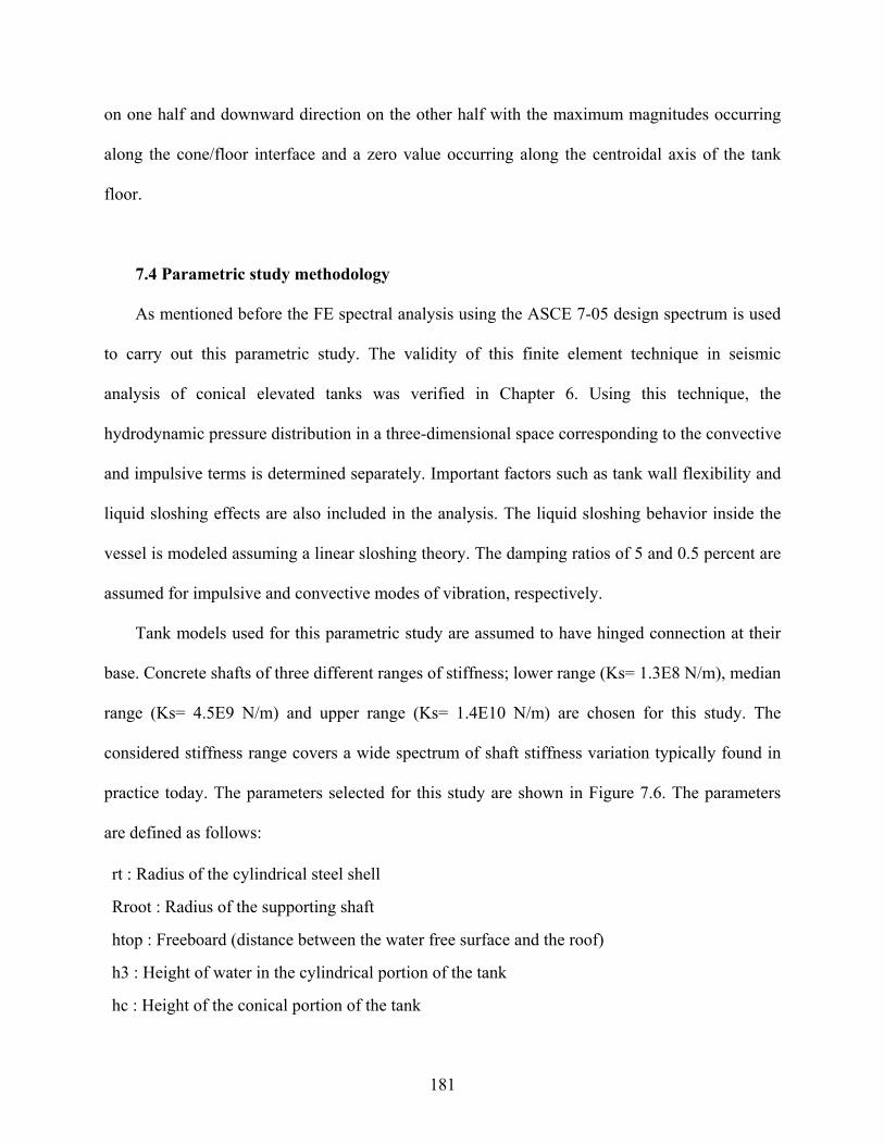
181

on one half and downward direction on the other half with the maximum magnitudes occurring

along the cone/floor interface and a zero value occurring along the centroidal axis of the tank

floor.

7.4 Parametric study methodology

As mentioned before the FE spectral analysis using the ASCE 7-05 design spectrum is used

to carry out this parametric study. The validity of this finite element technique in seismic

analysis of conical elevated tanks was verified in Chapter 6. Using this technique, the

hydrodynamic pressure distribution in a three-dimensional space corresponding to the convective

and impulsive terms is determined separately. Important factors such as tank wall flexibility and

liquid sloshing effects are also included in the analysis. The liquid sloshing behavior inside the

vessel is modeled assuming a linear sloshing theory. The damping ratios of 5 and 0.5 percent are

assumed for impulsive and convective modes of vibration, respectively.

Tank models used for this parametric study are assumed to have hinged connection at their

base. Concrete shafts of three different ranges of stiffness; lower range (Ks= 1.3E8 N/m), median

range (Ks= 4.5E9 N/m) and upper range (Ks= 1.4E10 N/m) are chosen for this study. The

considered stiffness range covers a wide spectrum of shaft stiffness variation typically found in

practice today. The parameters selected for this study are shown in Figure 7.6. The parameters

are defined as follows:

rt : Radius of the cylindrical steel shell

Rroot : Radius of the supporting shaft

htop : Freeboard (distance between the water free surface and the roof)

h3 : Height of water in the cylindrical portion of the tank

hc : Height of the conical portion of the tank

182

hshaft : Height of the supporting shaft

tcyl : Average thickness of the cylindrical portion of the tank

tcon : Average thickness of the conical portion of the tank

tfloor : Thickness of the tank’s floor

tshaft : Thickness of the concrete shaft wall

teta : Cone angle

Figure 7.6 Parameters defined for the parametric study

In total, 243 elevated tank models were created throughout this parametric study. On each

model, two different types of analysis; modal and spectral were performed. The tank

configurations considered for this study cover “Rroot/h3” ratios varying from 0.40 to 1.30, and

“hc/h3” ratios varying from 0.40 to 1.00. This results in a wide range of tank capacities

encompassing form the smallest to the largest conical elevated tanks ever built in practice. It

should be noted that for the cone angle "teta" to remain at 45°, the ratio of “rt/h3” should be

183

selected equal to the summation of the ratios “hc/h3” and “Rroot/h3” for each tank configuration

under consideration.

The value of parameter “htop” is considered to be equal to 0.50 m for all elevated tank

models analyzed. In addition, the value of parameter “teta” is kept constant at 45° for all models

considered throughout this parametric study.

FE models are created using the parametric model specifically written for this parametric

study using the ANSYS command lines. Detailed discussion on this parametric model can be

found in Appendix B.

For all models, the mass densities of 1000 kg/m3, 7898 kg/m3, and 2400 kg/m3 are assumed

for water, steel, and concrete materials, respectively. All structural parts are modeled assuming

linear elastic material. The Young's modulus of 200 GPa and 24.86 GPa are used for steel and

concrete materials, respectively. Furthermore, Poisson's ratios corresponding to steel and

concrete materials are assumed to be 0.30 and 0.16, respectively. The stored fluid is modeled

using eight-node brick fluid elements and the structural domain is modeled using four-node

quadrilateral shell elements having six degrees of freedom (translations and rotations) per node.

Based on the results obtained from this parametric study, a number of pressure graphs

presenting the pressure distribution along the height of the tank wall are determined for both

convective and impulsive components. The graphs are plotted as normalized wall pressure

(Pc/Sac/WL) or (Pi/Sai/WL) versus water depth ratio (h/hl), where “Pc” and “Pi” represent the

convective and impulsive pressure values in N/m2, respectively. “Sac” and “Sai” are the spectral

accelerations in m/s2 corresponding to the convective and impulsive modes, respectively. “WL”

is the weight of the contained water in Newton (N) and “hl” is the height of the water inside the

tank in meter (m).

184

In plotting these pressure graphs, the values of spectral accelerations (Sai and Sac) were

calculated based on the ASCE 7-05 design spectrum using the natural periods of impulsive and

convective modes, respectively obtained from the FE modal analysis. In doing so, the values of

“Importance factor” I=1 and “Response modification coefficient” R=1 were chosen as per ASCE

7-05. Furthermore, the mapped spectral accelerations ( SS and 1S ) were selected as 1.5g and o.6g,

respectively. Site class "A", representing a site with hard rock soil was also assumed in

determining these accelerations.

7.5 Sensitivity studies

Prior to performing the parametric study, a set of sensitivity analyses were carried out to

investigate the sensitivity of the proposed quantities (Pc/Sac/WL) and (Pi/Sai/WL) to different

parameters such as floor thickness “tfloor“ and plate thickness along the cylindrical “tcyl“ and

conical “tcon“ portions of the vessel.

7.5.1 Effect of floor thickness variation

In order to examine the effect of floor thickness variation on the normalized pressure

distribution, three different tank models having different floor thicknesses are considered. The

assumed tank models have the following properties in common:

h3 = 6.85 m, hc = 4.28 m, hshaft = 22.0 m, htop = 0.5 m, rt = 12.42 m,

Rroot = 8.13 m, tcyl = 8.83 mm, tcon = 24.51 mm, tshaft = 381 mm.

The tank has the full capacity of 4755 m3 (1.26 MG). Three different values of floor

thickness “tfloor” equal to 250 mm, 330 mm, and 450 mm are chosen and the resulting

185

normalized pressure distribution corresponding to the convective (Pc/Sac/WL) and impulsive

(Pi/Sai/WL) components along the height of the tank wall are calculated (see Figure 7.7).

-1.0

-0.8

-0.6

-0.4

-0.2

0.0 0.1 0.2 0.3 0.4 0.5

Normalized wall pressure (Pc/Sac/WL)*103, s2/m3

Wa

ter

dep

th r

atio

(h/h

l)

Floor thickness= 330 mm



h/hl=-0.615

Cone/Cylinder interface

(a)

-1.0

-0.8

-0.6

-0.4

-0.2

0.0

0.0 0.1 0.2 0.3

Normalized wall pressure (Pi/Sai/WL)*103, s2/m3

Wat

er

de

pth

rat

io (

h/h

l)

Floor thickness= 330 mmFloor thickness= 250 mmFloor thickness= 450 mm

h/hl=-0.615Cone/Cylinder interface

(b)

Figure 7.7 Pressure distribution over the tank wall (Effect of floor thickness variation);


As obvious from Figure 7.7, normalized pressure distribution is almost independent of the

floor thickness variation. This trend is observed for both convective and impulsive response

components.

186

7.5.2 Effect of plate thickness variation

In this section the effect of plate thickness variation on the normalized pressure distribution

is investigated by selecting three different tank models having different plate thicknesses. The

following properties are common to the three elevated tank models considered:

h3 = 6.85 m, hc = 4.28 m, hshaft = 22.0 m, htop = 0.5 m, rt = 12.42 m,

Rroot = 8.13 m, tshaft = 381 mm, tfloor = 330 mm.

The geometry of the tank is the same as that explained in the previous subsection. However,

in order to examine the effect of plate thickness variation on the proposed normalized pressure

quantity, three different values of plate thicknesses “tcyl” and “tcon” are chosen.

As mentioned above, three different tank models are created by doubling (2t) and halving

(0.5t) the plate thicknesses “tcyl” and “tcon”. The original plate thicknesses (t) corresponding to

the cylindrical and conical portions of the vessel are 8.83 mm and 24.51 mm, respectively. The

resulting normalized pressure distributions along the height of the tank wall corresponding to

these three models are indicated in Figure 7.8. Consequently, as indicated in Figure 7.8, the

proposed normalized pressure quantity can be considered independent of the plate thickness

variation. This is true for both convective and impulsive terms.

As a result, it can be concluded that by normalizing the obtained pressure values with

respect to the spectral accelerations (Sac and Sai), one can omit the sensitivity of the

hydrodynamic pressure to the variation of floor and plate thicknesses. This reduces the number

of parameters required to perform the parametric study yielding considerable reduction in

computational efforts.

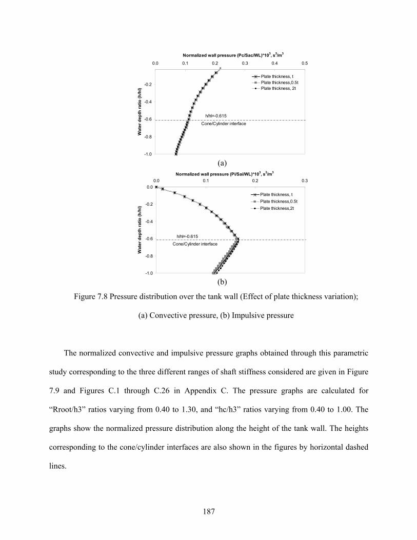
187

-1.0

-0.8

-0.6

-0.4

-0.2

0.0 0.1 0.2 0.3 0.4 0.5


Wa

ter

dep

th r

atio

(h/h

l)

Plate thickness, tPlate thickness,0.5tPlate thickness, 2t

h/hl=-0.615


(a)

-1.0

-0.8

-0.6

-0.4

-0.2

0.0

0.0 0.1 0.2 0.3


Wat

er

de

pth

rat

io (h

/hl)

Plate thickness, t

Plate thickness,0.5t

Plate thickness,2t

h/hl=-0.615


(b)

Figure 7.8 Pressure distribution over the tank wall (Effect of plate thickness variation);


The normalized convective and impulsive pressure graphs obtained through this parametric

study corresponding to the three different ranges of shaft stiffness considered are given in Figure

7.9 and Figures C.1 through C.26 in Appendix C. The pressure graphs are calculated for

“Rroot/h3” ratios varying from 0.40 to 1.30, and “hc/h3” ratios varying from 0.40 to 1.00. The

graphs show the normalized pressure distribution along the height of the tank wall. The heights

corresponding to the cone/cylinder interfaces are also shown in the figures by horizontal dashed

lines.

188

-1.0

-0.8

-0.6

-0.4

-0.2

0.0 0.1 0.2 0.3 0.4 0.5 0.6


Wat

er d

epth

rat

io (

h/h

l)1.30

1.19

1.080.96

0.85 0.74

0.630.51

Rroot/h3=0.40

h/hl=-0.714


(a)

-1.0

-0.8

-0.6

-0.4

-0.2

0.0

0.0 0.1 0.2 0.3 0.4 0.5 0.6 0.7


Wat

er d

epth

rat

io (

h/h

l)

h/hl=-0.714


1.30

1.19

1.08

0.96

0.85 0.74 0.63 0.51 Rroot/h3=0.40

(b)

Figure 7.9 Pressure distribution over the tank wall for Ks= 4.5E9 N/m and hc/h3=0.4;


As shown in the figures, it can be noticed that as the Rroot/h3 ratio increases, the normalized

impulsive wall pressure decreases gradually while keeping a similar pressure distribution pattern

over the tank height. Observing the given convective pressure graphs, it can be noted that an

189

increase in the Rroot/h3 ratio results in a decrease in the normalized convective wall pressure for

the upper sections of the tank, whereas a reverse trend is observed for the lower sections.

Moreover, it can be noticed that the convective pressure reaches its maximum value at the water

free surface while the impulsive pressure reaches its peak value at the cone/cylinder interface

with the zero magnitude occurring at the fee surface.

7.6 Verification study

In order to examine if the proposed pressure graphs are capable of estimating the seismic

response of liquid-filled conical elevated tanks accurately; a verification study is conducted on

two randomly selected elevated tank models.

7.6.1 Elevated tank model A

The tank configuration considered for this part of verification study is that of an actual

elevated tank situated in the U.S. The selected tank is a 1945 m3 elevated water storage tank with

dimensions as specified in Figure 7.10. Hinged boundary condition is assumed at the base of the

tank. Other geometric properties not indicated in the figure are expressed below:

side shell thickness: 6.9 mm

cone thickness: 11.4 mm

tank floor thickness: 533 mm

shaft thickness: 300 mm

A distributed mass (total mass 115×103 kg) accounting for the equivalent mass of the

platforms inside the pedestal with their full live load is applied at 20.3 m above the base. In

addition, a distributed mass balance of 111×103 kg accounting for the mass of the components of

190

the tank (e.g. roof, access tube, etc.) is assigned at the ring beam level. The material properties

defined for water, concrete and steel parts of the model are as explained before under section 7.4

of this chapter. The finite element idealization of the tank is also indicated in Figure 7.10.

(a) (b)

Figure 7.10 Elevated tank model A; (a) Tank geometry, (b) 3D FE model

The peak values of shear and overturning moment at the base of the tank due to lateral

seismic excitation are obtained using three different methods; FE time-history analysis, “current

practice” method (described under section 6.2.1.1), and finally the method presented in this

chapter using the proposed parametric pressure graphs. The response values are obtained for

191

convective and impulsive components separately. The results of FE-time history analysis are

used to assess the adequacy of the other two methods mentioned above.

The same FE technique as that explained previously in Chapter 6 is utilized here for

determining the transient response of the selected elevated tank model under a random ground

excitation. The validity of this method was verified formerly in Chapter 6.

The tank is subjected to the horizontal component of 1940 El-Centro ground motion with the

peak ground acceleration of 0.32g. The earthquake record is shown in Figure 6.8. The direct

integration method with an integration time step of 0.005 second is used. Sloshing effect is also

included in the time history analysis. The damping ratios of 5 and 0.5 percent are assigned for

impulsive and convective components, respectively. Moreover, the damping ratios of 5 and 2

percent are assumed as structural damping for concrete and steel parts of the tank model,

respectively. Figure 7.11 illustrates the time history results for the elevated tank model. The

maximum absolute response values obtained through FE time-history analysis are given in Table

7.1.

-6.0E+03

-4.0E+03

-2.0E+03

0.0E+00

2.0E+03

4.0E+03

6.0E+03

0 10 20 30 40

Time(s)

Bas

e S

hea

r (k

N)

-2.0E+05

-1.5E+05

-1.0E+05

-5.0E+04

0.0E+00

5.0E+04

1.0E+05

1.5E+05

2.0E+05

0 10 20 30 40

Time(s)

Ba

se

Mo

me

nt

(kN

m)

(a) (b)

Figure 7.11 Impulsive time history results for the elevated tank model A; (a) Base shear,

(b) Base moment

192

Table 7.1 Peak base shear and base moment response values for the elevated tank model A

FE time-history Current practice Pressure graphs

Convective Impulsive Convective Impulsive Convective Impulsive

Max value

Ratio Max value

Ratio Max value

Ratio Max value

Ratio Max value

Ratio Max value

Ratio

Base shear (kN)

723 1.00 4865 1.00 687 0.95 4968 1.02 743 1.03 5332 1.09

Base moment (kN.m)

30747 1.00 182080 1.00 30208 0.98 195727 1.07 30942 1.01 200275 1.10

Using the two-mass idealization approach recommended by “current practice”, two modes

of vibration with the natural periods of 4.21 sec and 1.01 sec corresponding to the fundamental

convective and impulsive modes, respectively are identified. These period values are in excellent

agreement with the natural periods of 4.23 sec and 1.11 sec obtained from a modal FE analysis.

In calculating the response values using the current practice method, the values of

“Importance factor”, I=1 and “Response modification coefficient” R=1 are used. Furthermore,

the design spectrum scaled to a peak ground acceleration of 0.32g to correspond with the

earthquake record used in FE time-history analysis is employed. The mapped spectral

accelerations ( SS and 1S ) for Imperial Valley location are determined as 1.5g and o.6g,

respectively per ASCE 7-05. Moreover, site class “A” representing a site with hard rock soil is

chosen to correspond with the rigid ground boundary condition assumed in FE modeling of the

tank.

Using the formulations given in section 6.2.1.1, one can calculate the base shear values of

687 kN and 4968 kN corresponding to the convective and impulsive terms, respectively.

Furthermore, based on the current practice approach, the base moment values of 30208 kNm and

195727 kNm are found for convective and impulsive components, respectively. The calculated

193

convective and impulsive terms may be combined by SRSS method to determine the total

response values of the tank-pedestal system.

As a third and final method, the seismic response of the elevated tank model is calculated by

applying the appropriate pressure values obtained from the proposed pressure graphs. The

selected tank model has the shaft stiffness of about 1.3E8 N/m, and the aspect ratios Rroot/h3

and hc/h3 of 0.43 and 0.42, respectively. Therefore, the appropriate pressure values are obtained

by interpolating between the values determined from the curves corresponding to the aspect

ratios of Rroot/h3=0.4 and 0.51 and also hc/h3=0.4 and 0.475. In interpolating the pressure

values, graphs corresponding to the shaft stiffness of Ks= 1.3E8 N/m are used.

Entering the natural periods of 4.23 sec and 1.11 sec corresponding to the fundamental

convective and impulsive modes, respectively into the El-Centro response spectrum, the spectral

acceleration of Sai=0.27g for impulsive and Sac=0.06g for convective mode are obtained. The

5% and 0.5%-damped response spectra scaled to the peak ground acceleration of 0.32g are used

for impulsive and convective modes, respectively. Substituting these spectral accelerations (Sai

and Sac) along with the weight of stored water (WL) into the normalized pressure values

obtained from interpolation, the actual hydrodynamic pressure values can be computed. The

resulting convective and impulsive pressures are shown in Figure 7.12.

As shown in the figure, the convective pressure has the peak value of 6.2 kPa at water free

surface, while the impulsive pressure has the peak value of 21.8 kPa at cone/cylinder interface.

For the sake of simplicity, the equivalent linear approximation may be used instead of the exact

pressure distribution by equating the area under the exact pressure distribution curve to the area

under the idealized linear approximation curve, as indicated in Figure 7.12.

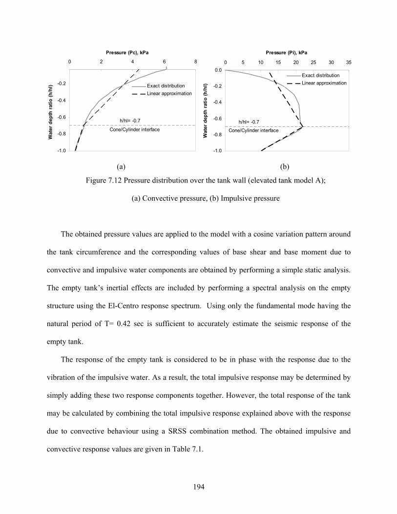
194

-1.0

-0.8

-0.6

-0.4

-0.2

0 2 4 6 8

Pressure (Pc), kPaW

ater

dep

th r

atio

(h

/hl) Exact distribution

Linear approximation

h/hl= -0.7


-1.0

-0.8

-0.6

-0.4

-0.2

0.0

0 5 10 15 20 25 30 35

Pressure (Pi), kPa

Wat

er d

epth

rat

io (

h/h

l)

Exact distribution


h/hl= -0.7


(a) (b)

Figure 7.12 Pressure distribution over the tank wall (elevated tank model A);


The obtained pressure values are applied to the model with a cosine variation pattern around

the tank circumference and the corresponding values of base shear and base moment due to

convective and impulsive water components are obtained by performing a simple static analysis.

The empty tank’s inertial effects are included by performing a spectral analysis on the empty

structure using the El-Centro response spectrum. Using only the fundamental mode having the

natural period of T= 0.42 sec is sufficient to accurately estimate the seismic response of the

empty tank.

The response of the empty tank is considered to be in phase with the response due to the

vibration of the impulsive water. As a result, the total impulsive response may be determined by

simply adding these two response components together. However, the total response of the tank

may be calculated by combining the total impulsive response explained above with the response

due to convective behaviour using a SRSS combination method. The obtained impulsive and

convective response values are given in Table 7.1.

195

As presented in Table 7.1, in general using both “current practice” and proposed pressure

graphs has resulted in a precise estimation of base shear and base moment values under both

convective and impulsive vibrations. However, current practice has underestimated the

convective base shear and base moment by about 5% and 2%, respectively.

Utilizing the proposed pressure graphs has led to a slight overestimation of the convective

base shear and base moment by only 3% and 1%, respectively. This approach also produces a

reasonable overestimation of the impulsive base shear and base moment of approximately 9%

and 10%, respectively which seems appropriate for design applications.

7.6.2 Elevated tank model B

The elevated tank model considered for this part is the same tank that was described in

Chapter 6, section 6.2.3. The chosen tank has the water storage capacity of 7571 m3. All

properties of the tank model are given in Chapter 6. Similar to previous section, the peak values

of base shear and base moment are determined using three different approaches; FE time-history

analysis, “current practice” method, and the method presented in this chapter using the proposed

parametric pressure graphs. The horizontal component of 1940 El-Centro ground motion with

the peak ground acceleration of 0.32g is applied to the model as lateral excitation. The damping

ratios of 5 and 0.5 percent are used for impulsive and sloshing components, respectively. The

maximum absolute response values obtained through three different approaches are given in

Table 7.2.

Similar to the procedure described in previous section, one can calculate the base shear

values of 2156 kN and 32778 kN using current practice corresponding to the convective and

196

impulsive terms, respectively. Based on the current practice approach, the base moment values

of 91588 kNm and 1215668 kNm are obtained for convective and impulsive terms, respectively.

Table 7.2 Peak base shear and base moment response values for the elevated tank model B

FE time-history Current practice Pressure graphs

Convective Impulsive Convective Impulsive Convective Impulsive

Max value

Ratio Max value

Ratio Max value

Ratio Max value

Ratio Max value

Ratio Max value

Ratio

Base shear (kN)

2487 1.00 35548 1.00 2156 0.87 32778 0.92 2661 1.07 38036 1.07

Base moment (kN.m)

94023 1.00 1320592 1.00 91588 0.97 1215668 0.92 98724 1.05 1465857 1.11

As a third approach, the seismic response of the elevated tank model is determined by

applying the appropriate pressure values obtained from the proposed pressure graphs. The

selected tank model has the shaft stiffness of about 4.5E9 N/m, and the aspect ratios Rroot/h3

and hc/h3 of 1.3 and 0.90, respectively. Therefore, the appropriate pressure values are calculated

by interpolating between the values determined from the curves corresponding to the aspect

ratios of hc/h3=0.85 and 0.925. In interpolating the pressure values, graphs corresponding to the

shaft stiffness of Ks= 4.5E9 N/m and aspect ratio of Rroot/h3=1.3 are used.

Entering the natural periods of 6.2 sec and 0.51 sec corresponding to the fundamental

convective and impulsive modes, respectively into the El-Centro response spectrum, the spectral

acceleration of Sai=0.88g for impulsive and Sac=0.067g for convective mode are obtained. The

5% and 0.5%-damped response spectra scaled to the peak ground acceleration of 0.32g are used

for impulsive and convective modes, respectively. Substituting these spectral accelerations (Sai

and Sac) along with the weight of stored water (WL) into the normalized pressure values

197

obtained from interpolation, the actual hydrodynamic pressure values can be computed. The

resulting convective and impulsive pressures are shown in Figure 7.13.

-1.0

-0.8

-0.6

-0.4

-0.2

0 2 4 6 8 10 12

Pressure (Pc), kPa

Wat

er d

epth

rat

io (

h/h

l)

Exact distribution



-1.0

-0.8

-0.6

-0.4

-0.2

0.0

0 20 40 60 80 100

Pressure (Pi), kPa

Wat

er d

epth

rat

io (

h/h

l)

Exact distribution


h/hl= -0.53


(a) (b)

Figure 7.13 Pressure distribution over the tank wall (elevated tank model B);


As shown in the figure, the convective pressure has the peak value of 8.2 kPa at water free

surface, while the impulsive pressure has the peak value of 68.6 kPa at cone/cylinder interface.

The equivalent linear approximation is also indicated in the figure. Similar to the procedure

described in the previous section, one can calculate the corresponding values of base shear and

base moment due to convective and impulsive components by applying the obtained pressure

values to the model. The calculated values are listed in Table 7.2.

As presented in Table 7.2, an accurate estimation of results is obtained using the proposed

pressure graphs for both convective and impulsive response components of the medium-capacity

tank model under consideration. Employing the proposed pressure graphs has resulted in a slight

overestimation of the convective base shear and base moment by only 7% and 5%, respectively.

198

A reasonable overestimation of around 7% and 11% is also obtained using this procedure for

impulsive base shear and base moment, respectively. As a result, a designer can use this

approach with confidence to accurately estimate the response values in seismic design of liquid-

filled conical elevated tanks.

7.7 Summary

In this chapter, a comprehensive parametric study was carried out on liquid-filled conical

elevated tanks using a detailed FE technique in a three-dimensional space. Based on the results

of this study, the convective and impulsive pressure values can be separately determined along

the height of the tank wall for typical elevated water tanks found in practice today.

In performing this parametric study, the effects of tank wall flexibility and sloshing of the

water free surface were considered. The study covered a wide range of tank dimensions and

geometries commonly found in current practice. The effects of deciding parameters such as shaft

stiffness, tank radius, shaft radius, height of contained water, tank height and so on were taken

into consideration in this parametric study.

Through this parametric study, the normalized pressure distribution graphs corresponding to

the convective and impulsive components were obtained for a wide range of varying parameters

by carrying out FE spectral analyses on a large number of conical elevated tanks. Spectral

analyses were performed using ASCE 7-05 design spectrum. The graphs were plotted as

normalized wall pressure (Pc/Sac/WL) or (Pi/Sai/WL) against water depth ratio (h/hl).

Based on the results of the sensitivity studies conducted, it was concluded that the proposed

normalized pressure quantities (Pc/Sac/WL and Pi/Sai/WL) were almost insensitive to the

variations of plate thickness along the cylindrical and conical portions of the vessel. This study

199

also demonstrated the independence of the proposed normalized pressure quantities from the

variations of tank’s floor thickness. Thus, it was concluded that the sensitivity of the

hydrodynamic pressure to the floor and plate thickness variations can be removed by

normalizing the hydrodynamic pressure with respect to the spectral accelerations.

In the first part of the chapter, the effect of inclusion of the roof on dynamic response of the

conical elevated tanks was investigated by carrying out FE analyses on an open-topped and a

roofed tank model and comparing the obtained response values. It was observed that the effect of

inclusion of the roof on dynamic response of such structures was insignificant and as a result its

effect was neglected throughout the parametric study.

A detailed explanation was provided on the exact pressure distribution patterns on the wall

and the floor of conical elevated tanks under lateral seismic excitations. This was achieved by

conducting a free vibration FE analysis on a typical liquid-filled elevated tank. Both convective

and impulsive modes of vibration were included for this part of the study.

The validity of the calculated pressure graphs was verified by performing a comparison

study between the proposed pressure graph method as the investigated method and the pre-

verified FE time history method as the control method. For comparison purposes, the obtained

results were also compared with those recommended by current practice. Based on the results of

this verification study, it was concluded that the proposed normalized pressure graphs could be

utilized with high level of accuracy for seismic design of liquid-filled conical elevated tanks.

200

CHAPTER 8

APPLICATION OF PERIOD ADJUSTMENT AND SEISMIC

ISOLATION TECHNIQUES TO CONICAL ELEVATED TANKS

8.1 Introduction

In the present chapter, the applicability of two techniques to liquid-filled conical elevated

tanks is investigated. These techniques are proposed by Kumieda (1976) which are used for

reducing the effect of seismic excitation being input to the structure. Two different techniques

will be proposed and their application to elevated water tanks will be addressed.

The chapter is divided into two main parts. In the first part of the chapter, the first technique

called “Natural period adjustment method” is introduced. In this technique, the seismic response

of the elevated tank model can be reduced by increasing its natural period far beyond the

predominant period of the input motion. This can be achieved by providing some soft portion

within the tank structure itself to extend its natural period. In other words, the earthquake

induced response of the structure is reduced by providing a more flexible structural design which

can in turn be accomplished by making alterations in tank’s configuration/geometry. The effect

of such modification on dynamic response of elevated water tanks is investigated in this study by

performing FE time-history analyses on various tank-pedestal models having different

configurations/geometries.

The second part of the chapter addresses the application of “isolation method” to liquid-

filled conical elevated tanks. In this technique, the supporting shaft structure is isolated either

from the ground or the vessel mounted on top by means of seismic isolators such as lead-rubber

201

and elastomeric bearings. Devices such as lead-rubber bearings may also be considered as energy

dissipaters which are capable of absorbing the input seismic energy.

The application of these two innovative menshin (earthquake reduction) techniques for

elevated water tanks will be investigated in detail throughout this chapter using a rigorous finite

element method (FEM). The proposed FEM is capable of simulating the accurate 3D behavior of

the isolated elevated tanks involving the nonlinear hysteretic behavior of seismic isolators.

8.2 Natural period adjustment method

The main focus of this section is on the effect of cone angle on the seismically induced

response of the supporting structure in liquid-filled conical elevated tanks. Finite element (FE)

technique is used to investigate such effect. This FE technique was explained in detail in

previous chapters in this thesis. Using this technique, the seismic behavior of elevated water

tanks having different cone angles under random excitation is investigated.

Effects of tank wall flexibility, damping properties of impulsive and convective components

of water, sloshing of the water free surface and both translational and rocking motions of the

supporting shaft are accounted for in the FE analysis. Moreover, the contribution of impulsive

and convective components of the response is accounted for separately.

The primary objective of this part of study is to evaluate the effect of the inclined cone angle

of the lower portion of the combined vessel on the dynamic behavior of the entire structure. In

the construction of vessels, the slope is usually assumed as 45°. The effect of varying slope

ranging from 45° to 90° is examined. To do so, the time history response of the considered tank-

pedestal models with different cone angles is obtained using modal superposition technique. The

selected elevated tank models are subjected to a unidirectional horizontal seismic excitation and

202

the corresponding transient base shear and base moment response values at the base of the shaft

structure are determined. Furthermore, to examine the accuracy of current practice a comparison

between the finite element results and those recommended by current practice is also made. The

current practice method is explained in detail under sections 6.2.1.1 and 6.2.5.

As per ACI 371R-08 (2008) for all models under consideration, a sufficient number of

modes (both impulsive and convective) to reach a cumulative modal mass participation of at

least 90% of the total mass of the system in the excitation direction are used.

In total, five elevated tank models are employed for FE analyses. The geometry and other

considerations taken into account in modeling of the tanks are described below.

8.2.1 Tank models

The elevated tank models considered in this study are assumed to have hinged condition at

the base. The original model (Model A) is a 7571 m3 (2 MG) actual elevated water tank located

in the U.S. Five different models are considered in which they have different cone angles but

with constant depth of water. Model A has a cone angle of 45°. Models B, C, D, and E are

created by increasing the angle (α) measured from the inclined cone interface of model A around

point A by 15, 30, 37.5, and 45 degrees, respectively. This results in cone angles (β) of 45, 60,

75, 82.5, and 90 degrees corresponding to models A, B, C, D, and E, respectively. The heights of

the cylindrical and conical portions of the vessels are kept constant. The tank floor cantilever

length (X) is then determined as a distance between the intersection point of cone-tank floor

center layers and the outer surface of the shaft. Therefore, by increasing the cone angle, the tank

floor cantilever length (X) is increased as shown in Figure 8.1. All models have the same shaft

height, shaft radius, and shaft thickness. Moreover, steel vessels of different models have similar

203

plate thicknesses, top cylinder radius, and cylindrical and conical heights. The simplified

geometry of the model is shown in Figure 8.1. All dimensions shown are in meters. Both modal

and time history analyses are carried out. Other properties of the model not indicated in the

figure including the properties assumed for the contained water, steel and concrete shell

materials are the same as those described in Chapter 6 under section 6.2.3.

For modeling the tanks, 16464 three-dimensional fluid elements along with a number of

shell elements ranging from 2996 to 3220 are used. For the sake of brevity, only the finite

element configurations of models A and C are indicated in Figure 8.2.

Figure 8.1 Simplified geometry of the elevated tank model

204

(a) (b)

Figure 8.2 FE idealizations of the models; (a) Model A, (b) Model C

8.2.2 Time history-modal analysis

The ground motion used for the time history analysis is the horizontal component of 1940

El-Centro earthquake scaled to the peak ground acceleration of 0.4g as shown in Figure 8.3. An

integration time step of 0.005 second is used for time history analysis of the tanks. In performing

the modal superposition analysis, the constant damping ratios of 3 and 0.5 percent are assigned

for impulsive and convective modes, respectively.

‐0.6

‐0.4

‐0.2

0

0.2

0.4

0.6

0 10 20 30 40 50 60

Time (Sec)

Acceleration (g)

Figure 8.3 Scaled 1940 El-Centro ground motion, horizontal component (PGA=0.4g)

205

The free vibration analysis results are listed in Table 8.1. The fundamental sloshing and

impulsive modes can be readily identified based on their high modal participation factors (β), as

indicated in the table. The modal participation factors are normalized with respect to the largest

participation factor among all modes of vibration. The ratio (Ri) given in the table is defined as

the ratio of the effective modal mass to the total mass of the system in the direction under

consideration. Water mass ratios and fundamental sloshing frequencies calculated from

Housner's method (Housner (1963)) are also given in the table. In using Housner's method, the

vessels are assumed to be rigid.

Comparing the mass ratios obtained for different models, it can be observed that by

increasing the cone angle from 45° to 90°, the convective mass ratio decreases gradually while

an inverse trend is observed for the impulsive mass ratio. This trend is similar for both FE and

Housner's methods. This is due to the fact that as the cone angle increases, the equivalent depth

of water (corresponding to the equivalent cylindrical model) increases too. As a result, a higher

aspect ratio (liquid height to diameter ratio “Hl/D”) is obtained for a model with a larger cone

angle which results in an increase in the impulsive mass and a decrease in the convective mass

ratios. This is a well-established relationship reported by many researchers (Housner (1963),

Haroun and Housner (1981A), and Veletsos (1984)) and standards (ACI 350.3-06).

By reviewing the table, it can be observed that the calculated FE results compare very well

with those given by Housner’s method which is based on the concept of equivalent cylinder

model. Such agreement is especially more noticeable between the computed natural frequencies.

In all cases considered, the difference in convective mass values is less than 5 percent of the total

mass of the contained water. A smaller difference of around 2 percent is observed for impulsive

masses.

206

Table 8.1 Free vibration analysis results for elevated tank models

Model A (45°) Mode Frequency(Hz) Effective mass

× 103 kg (FE) ∑Ri (%) β

(normalized) Number type FE Housner FE Housner

*1

Con

vect

ive 0.161

0.160 4302.51

58.7 56

1.00

2 0.161 235.38 0.23

3 0.294 NA 141.63 0.18

1

Impu

lsiv

e

1.955

NA

918.36

41.3 40.4

0.46

*2 1.955 3367.52 0.88

3 7.470 228.14 0.23

4 7.470 561.35 0.36

5 8.560 308.23 0.15

Model B (60°) Mode Frequency(Hz) Effective mass

× 103 kg (FE) ∑Ri (%) β


1

Con

vect

ive

0.162 0.163

48.63

57 53.3

0.10

*2 0.162 4696.61 1.00

3 0.294 NA

83.93 0.13

4 0.294 69.03 0.12

*1

Impu

lsiv

e

1.189

NA

3813.45

43 43.2

0.90

2 1.189 45.79 0.10

3 5.136 654.12 0.37

4 6.148 1410.52 0.55

Model C (75°) Mode Frequency(Hz) Effective mass

× 103 kg (FE) ∑Ri (%) β


1

Con

vect

ive

0.161 0.164

402.45 55.1 51.3

0.30

*2 0.161 4608.58 1.00

1

Impu

lsiv

e

0.816

NA

452.44

44.9 45.4

0.31

*2 0.816 2541.24 0.74

3 0.818 351.28 0.28

4 4.656 652.25 0.38

5 4.656 1546.66 0.58

6 5.683 440.91 0.31

* Fundamental mode

207

Table 8.1 Free vibration analysis results for elevated tank models (continued)

Model D (82.5°) Mode Frequency(Hz) Effective mass

× 103 kg (FE) ∑Ri (%) β


*1

Con

vect

ive

0.161 0.165 5110.99 54.9 50.46 1.00

1

Impu

lsiv

e

0.723

NA

129.54

45.1 46.4

0.16

*2 0.735 2895.07 0.75

3 0.740 177.19 0.19

4 4.354 2683.43 0.72

5 5.630 321.41 0.25

Model E (90°) Mode Frequency(Hz) Effective mass

× 103 kg (FE) ∑Ri (%) β


*1

Con

vect

ive

0.160 0.165

3621.79 54.6 49.6

1.00

2 0.160 1608.83 0.67

1

Impu

lsiv

e

0.662

NA

55.09

45.4 47.4

0.12

2 0.665 463.00 0.36

3 0.665 61.23 0.13

4 0.673 1888.41 0.72

5 0.675 389.36 0.33

6 0.675 81.81 0.15

7 4.098 1099.53 0.55

*8 4.098 1938.09 0.73

9 5.608 217.11 0.24

10 10.325 91.15 0.16

* Fundamental mode

It is important to note that all fundamental sloshing modes corresponding to models under

consideration have very close natural frequencies, however the effect of cone angle variations on

the natural frequencies of the impulsive modes is more pronounced. This is because of the

significant influence of cone angle variation on the relative stiffness distribution of structural

208

components which results in introducing new types of modes with different dynamic

characteristics to the tank-pedestal system.

From the results given in Table 8.1, one can conclude that for all considered models, the

sloshing behaviors of the models are almost dominated by their fundamental sloshing modes.

However, this is not the case for the impulsive response of the models having relatively large

cone angles (models C, D, and E). Calculated results show that for models A and B, fundamental

impulsive modes dominate the impulsive response. However, in models C, D, and E with larger

cone angles there are some modes having high contributions to the response that are not

necessarily fundamental modes (having the highest participation factor). For example, in model

D, the 4th mode has an impulsive mass participation very close to that of the fundamental mode

(2nd mode). Therefore considering more impulsive modes other than the fundamental mode

seems necessary in predicting the response of such models to horizontal ground motions.

It is found that all obtained impulsive modes for models A and B are translational modes. On

the other hand, the fundamental modes of models C and D and also 4th mode of model E which

has a very close effective mass and participation factor to that of the fundamental mode (mode 8

which is translational) are rocking type modes. The 5th mode of model C and 4th mode of model

D which have the second highest participation factors among all impulsive modes are

translational modes.

Considering the modal information given, one can conclude that the increase of cone angle

(which corresponds to the increase of the unsupported cantilever length between the shaft wall

and the cone shell) leads to introducing some rocking type modes (models C, D, and E) with

high values of participation factors and effective mass ratios to the system.

209

As shown in Table 8.1, these rocking modes with high contributions to the response have

relatively low natural frequencies compared to the typical translational modes and therefore have

small associated response spectrum accelerations. Consequently, it is expected that the resultant

base shear and overturning moment values of models with dominant rocking components

(models C, D, and E) be smaller than those with dominant translational components (models A

and B). This is further investigated in the next section by performing time history analyses on the

models. For the sake of brevity, only a few number of mode shapes are presented in Figure 8.4.

For a better view of the rocking mode shapes, only the associated shell deformations are

displayed.

For quantitative comparison of the seismic response of considered models under random

excitations, the time history values of base shear (V) and base moment (M) of the tank models

subjected to El-Centro earthquake are obtained using the modal superposition technique. The

modes listed in Table 8.1 are used to carry out such analyses. Time history results are separated

into impulsive and convective terms. As a result, the maximum response values associated with

each component (impulsive or convective) can be determined separately. Figures 8.5 and 8.6

illustrate the obtained time history results for all elevated tank models considered. The maximum

absolute response values computed from the FE analysis are listed in Table 8.2. Given in the

table, are also the maximum absolute response values normalized with respect to the total

effective weight of the system (We).

Reviewing the obtained results listed in Table 8.2 reveals that cone angle variations could

have a significant effect on the impulsive response of the system, however this effect is found to

be negligible for the convective component. Comparing the normalized base shear and base

moment ratios, it is further concluded that as expected model A with total base shear and base

210

moment ratios of 53.15% and 19.74 has the highest reaction forces compared to other models.

On the other hand, model C with total base shear and base moment ratios of 22.84% and 6.58 has

the lowest response values. The base shear and base moment of model C are only 43 and 33

percent of those of model A, respectively.

(a) (b)

(c) (d)

Figure 8.4 Fundamental mode shapes of elevated tanks; (a) Convective mode of Model A

(side view), (b) Impulsive mode (Translational) of Model A, (c) Convective mode of Model C

(3D view), (d) Impulsive mode (Rocking) of Model C

211

-6.0E+04

-4.0E+04

-2.0E+04

0.0E+00

2.0E+04

4.0E+04

6.0E+04

0 10 20 30 40 50 60

Time (sec)

Bas

e S

hea

r (k

N)

Convective

Impulsive

-6.0E+04

-4.0E+04

-2.0E+04

0.0E+00

2.0E+04

4.0E+04

6.0E+04

0 10 20 30 40 50 60

Time (sec)

Bas

e S

hea

r (k

N)

Convective

Impulsive

(a) (b)

-6.0E+04

-4.0E+04

-2.0E+04

0.0E+00

2.0E+04

4.0E+04

6.0E+04

0 10 20 30 40 50 60

Time (sec)

Bas

e S

hea

r (k

N) Convective

Impulsive

-6.0E+04

-4.0E+04

-2.0E+04

0.0E+00

2.0E+04

4.0E+04

6.0E+04

0 10 20 30 40 50 60

Time (sec)

Bas

e S

hea

r (k

N)

Convective

Impulsive

(c) (d)

-6.0E+04

-4.0E+04

-2.0E+04

0.0E+00

2.0E+04

4.0E+04

6.0E+04

0 10 20 30 40 50 60

Time (sec)

Bas

e S

hea

r (k

N)

Convective

Impulsive

(e)

Figure 8.5 Time history results for base shear; a) Model A, b) Model B, c) Model C,


212

-2.2E+06

-1.8E+06

-1.4E+06

-1.0E+06

-6.0E+05

-2.0E+05

2.0E+05

6.0E+05

1.0E+06

1.4E+06

1.8E+06

2.2E+06

0 10 20 30 40 50 60

Time (sec)

Bas

e M

om

ent

(kN

.m)

Convective

Impulsive

-2.2E+06

-1.8E+06

-1.4E+06

-1.0E+06

-6.0E+05

-2.0E+05

2.0E+05

6.0E+05

1.0E+06

1.4E+06

1.8E+06

2.2E+06

0 10 20 30 40 50 60

Time (sec)

Bas

e M

om

ent

(kN

.m)

Convective

Impulsive

(a) (b)

-2.2E+06

-1.8E+06

-1.4E+06

-1.0E+06

-6.0E+05

-2.0E+05

2.0E+05

6.0E+05

1.0E+06

1.4E+06

1.8E+06

2.2E+06

0 10 20 30 40 50 60

Time (sec)

Bas

e M

om

ent

(kN

.m) Convective

Impulsive

-2.2E+06

-1.8E+06

-1.4E+06

-1.0E+06

-6.0E+05

-2.0E+05

2.0E+05

6.0E+05

1.0E+06

1.4E+06

1.8E+06

2.2E+06

0 10 20 30 40 50 60

Time (sec)

Bas

e M

om

ent

(kN

.m) Convective

Impulsive

(c) (d)

-2.2E+06

-1.8E+06

-1.4E+06

-1.0E+06

-6.0E+05

-2.0E+05

2.0E+05

6.0E+05

1.0E+06

1.4E+06

1.8E+06

2.2E+06

0 10 20 30 40 50 60

Time (sec)

Bas

e M

om

ent

(kN

.m) Convective

Impulsive

(e)

Figure 8.6 Time history results for base moment; a) Model A, b) Model B, c) Model C,


213

Table 8.2 Maximum absolute time history response values

Model

Base Shear (kN)


Max value Ratio(%) (Vc/We)

Max value Ratio(%) (Vi/We)

Max value Ratio(%) (V/We)

A 3108 3.15 53322 54.05 52440 53.15

B 3258 3.07 48530 45.73 48196 45.41

C 3315 3.07 24818 23.02 24627 22.84

D 3366 3.03 25741 23.19 27264 24.56

E 3432 3.03 32606 28.85 31624 27.98

Model

Base Moment (kN.m)


Max value Ratio

(Mc/We) Max value

Ratio (Mi/We)

Max value Ratio

(M/We)

A 117529 1.19 1980888 20.07 1947499 19.74

B 121358 1.14 1541155 14.52 1528799 14.40

C 122526 1.13 716878 6.65 709801 6.58

D 124011 1.11 704841 6.35 782770 7.05

E 125973 1.11 819312 7.25 782356 6.92

8.2.3 Effect of tank geometry

Table 8.2 shows that the selected models may be categorized into high (models A and B)

and low (models C, D, and E) range of response values according to their normalized shear and

moment ratios. In model A, the shaft, the floor and the cone center layers intersect at a common

interface and as a result no relative rotations can occur between them. Because of the rigidity of

the supporting shaft in the axial direction relative to its lateral direction, no rocking mode can be

developed for such models (Model A and to some extent model B). The restraint against the

rotation at the tip of the shaft, provided due to the overturning moment exerted at the top of the

shaft, tends to increase the stiffness of the shaft. This increase in stiffness results in low natural

214

periods and therefore high response spectral accelerations (as can be observed for models A and

B in Table 8.1).

When the cantilever length of the tank floor is large enough (models C, D, and E), dominant

rocking modes with low natural frequencies and thus associated low response spectral

accelerations are formed.

The fundamental mode type (translational or rocking) associated with each model, mainly

depends on the proportion of lateral to rotational (at the base of the vessel) stiffness. Therefore,

the judgment of fundamental mode type needs a rigorous analysis as done here. For models C

and D, the rotational stiffness at the base of the vessel is smaller compared to the lateral stiffness

of the shaft, while model E has relatively smaller lateral stiffness in comparison with its

rotational stiffness. This is believed to be the reason as why the fundamental mode types of

models C and D are rocking while that of model E is translational. This justifies the slight

increase of normalized response ratios of model E relative to models C and D.

For all models considered, sloshing modes have a negligible contribution to the base shear

and base moment response values. Among all models considered, the maximum contribution to

the base shear response due to sloshing modes is observed in model A with the sloshing

contribution of around 3% of the total effective weight of the system. However, for the same

model the impulsive term is found to have a much higher contribution of around 54%.

Since the sloshing motion of the contained water is not in phase with the impulsive vibration

of the tank-liquid system, in some of the cases including the sloshing effects has led to a slight

reduction in the total response.

215

For comparison purposes, the peak base shear and base moment values obtained for all the

models are normalized with respect to those of model A for which the highest response values

are calculated (see Figure 8.7).

0.00

0.20

0.40

0.60

0.80

1.00

No

rmal

ized

Bas

e S

hea

r R

atio

Model A Model EModel DModel CModel B

Low response models

0.00

0.20

0.40

0.60

0.80

1.00

No

rmal

ized

Bas

e M

om

ent

Rat

io

Model A Model EModel DModel CModel B

Low response models

Figure 8.7 Normalized base shear and base moment ratios

Figure 8.7 shows that among the selected models, model C with the cone angle of 75° may

be introduced as the optimum case with its base shear and base moment values being the lowest

response values among all considered models. As presented in Table 8.2, the base shear and

base moment response of the shaft may be decreased by a factor of 2.3 and 3.0 respectively by

only increasing the cone angle from 45° (as in model A) to 75° (as in model C). This could lead

to a more economical design of the shaft structure and the supporting foundation system.

However, design considerations allowing for the probably large rotations associated with the

rocking component of the response should be accounted for.

216

8.2.4 Comparison with current practice

In this section a comparison study is carried out between the FE method and the current

practice in order to estimate the accuracy of the current practice in calculating the seismic

response of the elevated tanks.

In computing the results using the current practice approach, the design spectrum scaled to

the peak ground acceleration of 0.4g to match the seismic excitation used in FE time history

analyses is used. The values of “Importance factor” I and “Response modification coefficient” R

are considered as unity. Moreover, the mapped spectral accelerations ( SS and 1S ) for Imperial

Valley location are selected as 1.5g and o.6g, respectively. Site class "A", representing the hard

rock soil is also assumed.

Following the current practice procedure explained in sections 6.2.1.1 and 6.2.5 leads to the

total base shear and base moment values of 49243 kN and 1827092 kN.m, respectively for model

A. Comparing these values with those of FE method given in Table 8.2, it can be observed that

the current practice estimations are in reasonable agreement with those calculated through FE

analysis for model A. For both base shear and base moment, the difference between the

estimated results is only 6 percent. However, for models with dominant rocking behavior

(models C, D, and E), the current practice highly overestimates the results, for instance as high as

2.2 times greater than those of FE for the base shear response of model C. The reason for such

overestimation is that the current practice approach is not capable of accounting for the effect of

rocking component of motion on the dynamic response of the tanks. Therefore, designing such

models according to current practice will lead to an overdesign of the shaft structure and the

supporting foundation system. To avoid this, a detailed dynamic analysis capable of accounting

217

for both translational and rotational (rocking) degrees of freedom of the shaft seems to be

essential.

8.3 Seismic isolation method

8.3.1 Passive control bearings

Among different types of passive control devices, lead-rubber and elastomeric bearings are

more widely used in today’s practice. They offer a simple and economical solution for seismic

isolation of structures. They have many features suiting them for use as efficient seismic

isolators.

Elastomeric bearings are usually made with alternating relatively thin horizontal layers of

rubber bonded to horizontal steel plates. They are generally preferred over plain rubber pads

because of their superiority under compressive loads. The vertical stiffness of bearing is

increased by the presence of these steel plates resulting in a relatively large overall vertical

stiffness. However, a low level of horizontal stiffness is provided by the rubber layers under the

lateral loads such as earthquake, wind, etc. Steel plates do not considerably change the shear

stiffness.

A lead-rubber bearing is manufactured by inserting a lead plug down the centre of a

laminated elastomeric bearing. This introduces a significant amount of hysteretic damping to the

bearing leading to further improvement in the reduction of forces and moments. The lead

material yields under a rather low level of shear stress and shows nearly an elastic-plastic

behavior (Robinson (1982)). It also shows a good fatigue behavior under cyclic loading. Rubber

bearings (both elastomeric and lead-rubber bearings) also increase the resonant period of the

structure to a value out of the range of the ground motion’s strong excitation. Lead-rubber

218

bearings provide the required amount of damping and the seismic isolation solution both in a

single unit. This yields a cheap solution to the problems of seismic isolation.

There have been a number of experimental studies on the behavior of lead-rubber bearings

in the past. However, only a few analytical research studies have been carried out on this type of

isolators. This is because of the difficulties associated with modeling the lead-rubber bearings.

Lead-rubber bearings consist of three different materials having different characteristics and

behaviors. The main difficulty encountered in the modeling process of lead-rubber bearings

results from the high nonlinearity of lead and rubber materials, incompressibility of rubber

material, and also geometric nonlinearities associated.

8.3.2 Nonlinear modeling of rubber material

The behavior of rubber-like material is very complex. They usually behave elastically

isotropic and can undergo large strains during a seismic event. The stress-strain relationship of

rubber material can be highly nonlinear. The behavior of such materials can be accurately

simulated by utilizing the hyperelastic models. Hyperelasticity is used for the materials capable

of experiencing large elastic strain that is recoverable to the initial state. As a result, elastomers

such as rubber and many other polymer materials can be considered in this category. Modeling

of the nonlinear characteristics of rubber material can be achieved based on the theory of finite

deformation.

There are several material constitutive models for modeling the isotropic behavior of the

rubber material. The strain energy potentials are usually used to define the constitutive behavior

of hyperelastic materials. The material is assumed to be purely incompressible. Assuming that

the material behavior is isotropic, the strain energy potential can be conveniently expressed in

219

terms of principal stretch ratios (Simo and Hughes (1997)). In this study, the Ogden Potential

constitutive model is used for large-strain analysis of rubber-like material (Ogden (1984) and

Ogden (1986)). In hyperelastic models, the strain energy potential function (W) can be assumed

to be a scalar function of one of the strain or deformation tensors. The derivative of the strain

energy potential with respect to a strain component gives the corresponding stress component.

The Ogden type of strain energy potential is expressed as:

N

k

k

k

N

i i

i Jd

W iii

1

2321

1

)1(1

)3(

(8-1)

where,

N = the order of the Ogden Potential function

kii d,, = material constants

J = the ratio of the deformed elastic volume over the undeformed volume of material (for

incompressible material J = 1)

1 , 2 , 3 = modified principal stretch ratios

Usually, a higher N result in a better fit the exact solution; however orders of N > 3 may

cause numerical difficulty in fitting the material constants. In this study, the Ogden Potential

model of order 3 (N = 3) is used.

The principal stretch ratio is expressed as:

ii 1 (8-2)

where, i is the principal value of the engineering strain tensor in the ith direction.

The initial shear modulus of the material ( ) is defined as:

N

iii

12

1 (8-3)

220

The initial bulk modulus is given as:

1

2

dK (8-4)

Constant 1d can thus be considered as material incompressibility parameter. It is obvious

that the accurate estimation of results during a hyperelastic analysis highly depends on the

accurate assessment of the material constants given in Eq. (8-1). Rubber material constants are

usually derived using experimental stress-strain data. In the current study, the test data reported

by Treloar (Treloar (1944) and Treloar (1975)) are used to characterize the rubber material

constants. Treloar performed three different types of experiments; uniaxial tension, equibiaxial

tension, and pure shear on samples cut from a sheet of Vulcanized natural rubber. These test data

cover several modes of deformation and a wide range of strain values. The rubber material

constants are then fit using these test data in all three deformation states simultaneously.

Combination of test data from multiple deformation states improves the simulation of the

hyperelastic behavior of the material.

The nonlinear least squares fit analysis is performed in this study in order to determine the

rubber material constants. By carrying out this analysis, the Ogden Potential constants can be

calculated from experimental stress-strain data given by Treloar. In the least squares fit analysis

method, the sum of the squared error between experimental and theoretically predicted stress

values is minimized. The sum of the squared error can be expressed as follows:

2

1

))(( ji

n

i

Ei CTTE

(8-5)

in which:

E = least squares residual error

EiT = experimental stress values

221

)( ji CT = engineering stress values (function of material constants)

n = number of experimental data points

In order to minimize the above equation, the variation of the squared error should be set to

zero i.e. 0E . This results in a set of equations which can be solved simultaneously to

determine the hyperelastic material constants;

01

C

E, 0

2

C

E, . . . , etc.

The optimum material constants were calculated using the least squares fit optimization

methodology for the three types of Treloar’s test data (uniaxial tension, equibiaxial tension, and

pure shear) simultaneously. The optimal values of i and i are given in Table 8.3. Since the

incompressible material is assumed here for hyper rubber under consideration (i.e. J = 1), the

parameters kd in Eq. (8-1) have no effect on the stress computations and therefore need not to be

determined. Utilizing these constants, one can calculate the nominal stress (engineering stress)

for different values of engineering strain ( ) which are depicted in Figure 8.8 for the three

different deformation states. Indicated in the figure, are also the experimental data measured by

Treloar. As evident from these figures, the considered rubber material parameters lead to

superior fit to all three test data for the entire range of strains. This verifies the validity of the

assumed hyperelasticity model, the parameter identification scheme and the estimated rubber

material constants listed in Table 8.3.

222

(a)

(b)

(c) Figure 8.8 Stress-strain results for rubber material using three types of test data (N=3),

(a) uniaxial tension, (b) equibiaxial tension, (c) pure shear

Engineering strain 1 2 3 4

Stress (MPa)

0.5

1

1.5

Treloar’s experimental dataCurrent study (Ogden model)

Engineering strain 1 2 3

1

2

Stress (MPa)

Treloar’s experimental dataCurrent study (Ogden model)

Engineering strain

Stress (MPa)

2 4 6

2

4

6 Treloar’s experimental data

Current study (Ogden model)

223

Table 8.3 Optimal values of rubber constants using three test data simultaneously (N=3)

Material constant (Pa) Value

1 483387

1 1.52

2 -21634

2 -1.78

3 188

3 5.93

8.3.3 Verification study

8.3.3.1 FE modeling of lead-rubber and elastomeric bearings

In this section, numerical analysis using an elaborate finite element technique is performed

to analyze the behavior of rubber bearings subjected to a combination of compression and shear

forces. Solid 185 element from the ANSYS® library of elements is used for the 3D FE modeling

of the lead, steel, and rubber parts of the bearings. The element has eight nodes and three degrees

of freedom at each node (translations in x, y, and z directions). The element is capable of

modeling both plasticity and hyperelasticity behaviors. Solid 185 element is particularly

designed for simulating material behavior with high incompressibility such as purely or nearly

incompressible hyperelastic materials (high poisson’s ratio) and elastoplastic materials

(experiencing large plastic deformations). The element offers a variety of options in handling

incompressible hyperelastic material behavior. The Ogden type constitutive model explained in

the previous section is used here for simulating the nonlinear behavior of rubber.

The “classical bilinear kinematic hardening” plasticity algorithm is adopted to capture the

nonlinear behavior of mild steel and lead materials. This plasticity algorithm uses the Von Mises

yield criterion together with the kinematic hardening rule. The stress-strain behavior

corresponding to this plasticity option is plotted in Figure 8.9 (a). Indicated in the figure is also

224

the stress space for this plasticity algorithm. The surfaces indicated in Figure 8.9 (b) are the yield

surfaces, that is, any stress state inside the surface leads to an elastic response of the material (no

plastic strain is developed). In kinematic hardening rule, it is assumed that the size of yield

surface remains unchanged and as the yielding progresses the yield surface translates into stress

space, as shown in Figure 8.9 (c). The following properties are assumed for the steel, lead, and

rubber materials:

Steel material: Lead material: * Rubber material:


Tangent modulus= 20.5 GPa

Yield stress= 275MPa


Density= 7850 kg/m3


Tangent modulus= 45 MPa

Yield stress= 12 MPa


Density= 11300 kg/m3


Density= 1150 kg/m3

Initial shear modulus= 0.39MPa

* Other properties for rubber

material are given in Table 8.3.

(a) (b)

(c)

Figure 8.9 Bilinear kinematic hardening plasticity algorithm; (a) stress-strain behavior,

(b) yield surfaces, (c) kinematic hardening rule

225

8.3.3.2 Comparison of results with experimental data

In order to validate the FE implementation process, the results obtained through FE analysis

are compared with those measured through experiments. The boundary conditions defined for

the FE models are in conformity with the actual conditions of the test.

Two full-scale lead-rubber bearings with the experimental data available are analyzed here

using the proposed 3D FE procedure. The first bearing is a lead-rubber shear damper consisting

of a 100 mm-diameter lead core inserted in the center of a 356×356×140 mm elastomeric

bearing. The role of the lead core is to increase the initial stiffness of the bearing and also to

increase the capacity of the isolator to dissipate energy. The bearing consists of seven mild steel

plates with the thickness of 3-mm and six rubber layers with the thickness of 16mm. Two steel

plates with the thickness of 20 mm are attached to the top and bottom faces of the bearing. These

plates are intended to connect the bearing to the structure and also help distribute the applied

forces. The experiment on this bearing was reported by Robinson and Tucker (1981). The

simplified geometry of the bearing along with its corresponding FE model are shown in Figure

8.10.

First, an incremental load of 400 kN is applied vertically to the bearing. Then a lateral force

of 100 kN is applied on the uppermost steel plate with a given compressive load (400 kN) being

retained. All degrees of freedom of the nodes located on the lowermost steel plate boundary are

restrained. Automatic time stepping feature of the software is used during the solution process.

This feature automatically optimizes the number of loading sub steps required for obtaining the

solution according to the response frequency and the nonlinearity effects experienced during the

solution phase. If the convergence is not obtained during a specific load step, the algorithm

automatically retreats to the previous converged solution and adjusts the load increment size

226

accordingly so that convergence is reached. The force-displacement curves corresponding to the

experimental and numerical approaches are indicated in Figure 8.11. As shown in the figure, a

good correlation between FE and experimental results has been generally obtained. The FE

approach predicts a relatively stiffer response for the unloading part of the hysteretic loop.

(a)

(b)

Figure 8.10 “356×356×140” mm lead-rubber bearing; (a) simplified geometry, (b) 3D finite

element model

The deformed shape of the bearing corresponding to loading points A, B, and C indicated on

the force-displacement curve of the bearing is shown in Figure 8.12. Figure 8.12(a) indicates the

deformed shape of the bearing under pure compression. Figures 8.12(b) and (c) present the

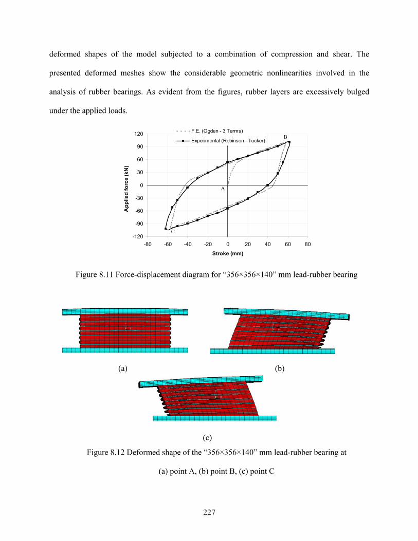
227

deformed shapes of the model subjected to a combination of compression and shear. The

presented deformed meshes show the considerable geometric nonlinearities involved in the

analysis of rubber bearings. As evident from the figures, rubber layers are excessively bulged

under the applied loads.

-120

-90

-60

-30

0

30

60

90

120

-80 -60 -40 -20 0 20 40 60 80

Stroke (mm)

Ap

plie

d fo

rce

(kN

)F.E. (Ogden - 3 Terms)

Experimental (Robinson - Tucker)

A

B

C

Figure 8.11 Force-displacement diagram for “356×356×140” mm lead-rubber bearing

(a) (b)

(c)

Figure 8.12 Deformed shape of the “356×356×140” mm lead-rubber bearing at

(a) point A, (b) point B, (c) point C

228

The second bearing is a large circular lead-rubber shear damper with the diameter of 650

mm and the height of 197mm. The bearing has a lead plug of 170 mm inserted in its center. The

simplified geometry of the bearing is presented in Figure 8.13. It consists of ten mild steel plates

with the thickness of 5-mm and nine rubber layers with the thickness of 15 mm. The experiment

on this bearing was reported by Robinson (1982). A high vertical load of 3.15 MN is applied first

using the automatic load increment size algorithm followed by the lateral force. The force-

displacement hysteretic loops corresponding to the experimental and numerical approaches are

shown in Figure 8.14. As obvious from the figure, a good agreement is generally obtained,

however the FE method estimates a stiffer behavior for the initial part of the loop (loading path)

but softer behavior for the unloading part.

The reasonable correlation between the FE simulation and the experimental results show the

adequacy of the employed hyperelasticity model, estimated material parameters, and employed

numerical procedure. As a result, when the experimental results are not available for the bearings

which are to be used in the structure, the proposed elaborate FE method can be used with

reasonable level of accuracy to predict the behavior of the isolator. This removes the need for

conducting tedious analytical and/or experimental studies.

Figure 8.13 Geometry of the 650 (Diameter) × 197 mm lead-rubber bearing

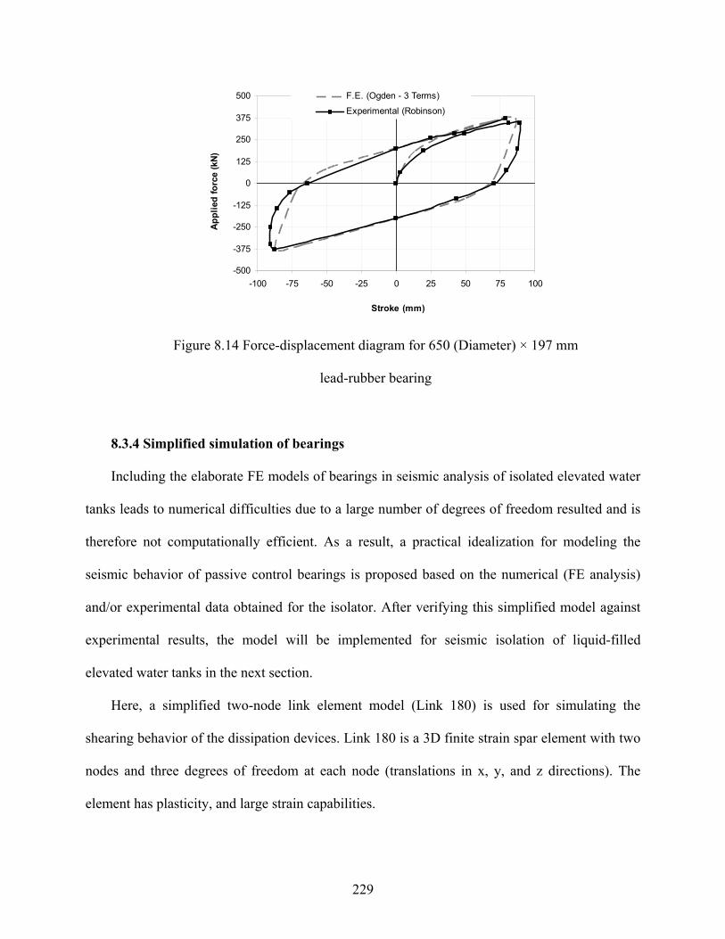
229

-500

-375

-250

-125

0

125

250

375

500

-100 -75 -50 -25 0 25 50 75 100

Stroke (mm)

Ap

pli

ed f

orc

e (k

N)

F.E. (Ogden - 3 Terms)

Experimental (Robinson)

Figure 8.14 Force-displacement diagram for 650 (Diameter) × 197 mm

lead-rubber bearing

8.3.4 Simplified simulation of bearings

Including the elaborate FE models of bearings in seismic analysis of isolated elevated water

tanks leads to numerical difficulties due to a large number of degrees of freedom resulted and is

therefore not computationally efficient. As a result, a practical idealization for modeling the

seismic behavior of passive control bearings is proposed based on the numerical (FE analysis)

and/or experimental data obtained for the isolator. After verifying this simplified model against

experimental results, the model will be implemented for seismic isolation of liquid-filled

elevated water tanks in the next section.

Here, a simplified two-node link element model (Link 180) is used for simulating the

shearing behavior of the dissipation devices. Link 180 is a 3D finite strain spar element with two

nodes and three degrees of freedom at each node (translations in x, y, and z directions). The

element has plasticity, and large strain capabilities.

230

The axial (vertical) behavior of the bearings (both elastomeric and lead-rubber bearings) is

modeled using a linear elastic spring element (Combin 14). The element has two nodes with up

to three degrees of freedom at each node (translations in x, y, and z directions). This allows the

effect of rocking motion to be accounted for in dynamic analysis of the tanks. Only a uniform

stress is allowed in the spring.

Based on the proposed simplified modeling technique, only a vertical stiffness (Kv) is

sufficient to characterize the axial behavior of the bearings. The horizontal (shearing) behavior of

the bearings is modeled using a bilinear kinematic hardening plasticity algorithm explained

before. As a result, three main parameters are needed to define the horizontal behavior of the

bearings; namely the yield strength (Qy), and the elastic (Ke) and plastic (Kp) stiffnesses.

Comparing to a typical stress-strain based plasticity algorithm, Qy corresponds to the yield

stress, and Ke and Kp correspond to the initial Young's modulus and tangent modulus,

respectively. A simplified hysteretic loop for lead-rubber bearings with the above parameters

indicated on is presented in Figure 8.15. The model parameters may be determined from an

elaborate FE analysis and/or an experimental study.

Figure 8.15 Simplified hysteretic loop for lead-rubber bearings

231

In the next section, the circular 650 (Diameter) × 197 mm lead-rubber bearings will be

incorporated for seismic isolation of elevated water tanks. The bearings will be simulated using

the simplified modeling technique explained here. Based on the experimental study by Robinson

(1982), the following parameters are suggested for simplified modeling of the bearing:

Qy = 224 kN , Ke = 17 mm

kN, Kp = 2

mm

kN, and Kv = 600

mm

kN.

The hysteretic behavior of the bearing is indicated in Figure 8.16 as determined by the

simplified approach and compared to the Robinson’s experimental data. As evident from the

figure, a reasonable agreement is observed between the results predicted by the simplified model

and experimental observations. As a result, this simplified model may be used for simulating the

behavior of rubber bearings without great loss of accuracy. The proposed model is practical,

straightforward and easy to use.

-500

-375

-250

-125

0

125

250

375

500

-100 -75 -50 -25 0 25 50 75 100

Stroke (mm)

Ap

pli

ed f

orc

e (k

N)

Experimental (Robinson)

Simplified model

Figure 8.16 Hysteretic loop for 650 (Diameter) × 197 mm lead-rubber bearing

(Simplified model)

232

8.3.5 Application to liquid-filled conical elevated tanks

8.3.5.1 General considerations

The application of passive control technique to liquid-filled conical elevated tanks, using

lead-rubber and elastomeric bearings in particular will be investigated in this section of the

thesis. The elevated tank model considered for this study is the same as that used in Chapter 6.

The properties of the model are described in detail under section 6.2.3. As explained in detail in

previous chapters, the fluid domain is modeled using eight-node 3D fluid elements and the

structural domain is modeled using four-node quadrilateral shell elements. Effects of both

impulsive and sloshing components of the stored water are included in the finite element

modeling of the tanks.

A total of forty eight 650 (Diameter) × 197 mm lead-rubber bearings are used for seismic

isolation of the tank models in this study. The hysteretic behavior of the bearing is explained in

the previous section and is indicated in Figure 8.16. It is worth noting that two nodes should be

defined at the locations of isolators in order to accommodate the isolation device where needed.

The number and properties of the bearings are chosen based on the Meggett (1978)

recommendations that reasonable values for the plastic shear stiffness and the yield strength of

lead-rubber pads should be taken as:

Kp = (1 to 2) W m -1 (8-6)

Qy = (0.05 to 0.10) W (8-7)

where, W is the part of the weight carried by the bearing. In the current study, the bearings

are measured with Kp ≈ 1.1 W m -1 and Qy ≈ 0.1 W. In a research study on the dynamic behavior

of isolated multi-storey buildings, Lee and Medland (1981) also suggested similar values to those

concluded by Meggett for plastic stiffness and yield strength of the bilinear hysteretic dampers.

233

Regarding the seismic isolation of bridges, Blakeley et al. (1980) proposed isolation parameters

close to those determined by Meggett.

Both modal and time history analyses are carried out on isolated and non-isolated elevated

tanks. The ground motion used for the time history analysis of the tanks is the horizontal

component of 1940 El-Centro ground motion with the peak ground acceleration of 0.50g. The

first 20 seconds of the record is used in dynamic analyses. Direct integration method is used for

transient analysis of the tanks.

As explained in detail in Chapter 4, the natural frequencies corresponding to the

fundamental convective and impulsive modes are used to determine the damping constants

( and ) in non-isolated tank problems. However, in the case of isolated tanks, since the

response is mainly dominated by the isolation mode, the natural frequency corresponding to this

mode should be used in determining the associated damping constant. The damping constant

associated with the sloshing component is determined using the natural frequency of the

fundamental convective mode, similar to what is done for non-isolated tanks. As will be

discussed later in this chapter, the fundamental sloshing frequency does not change significantly

due to seismic isolation.

The damping ratios equal to 0.5 and 5 percent are considered for the convective and

impulsive water components, respectively. The stiffness proportional damping equivalent to 5

and 2 percent of critical damping is considered as structural damping for concrete and steel

segments of the tank, respectively. In addition, the physical elastic-plastic hysteresis loss in

energy dissipation devices introduces a significant amount of damping to the system. The effect

of such damping is accounted for by defining an appropriate bilinear plasticity model for the

isolators. However, the viscous damping of isolators was neglected in FE modeling of the tanks

234

as the major part of the input seismic energy is dissipated by the hysteretic behavior of the

isolators.

In order to investigate the sensitivity of conical elevated tank response to seismic isolation

system, effects of various parameters such as lateral versus vertical isolation, location of

isolators, shaft stiffness, tank aspect ratio, and yield strength of isolators will be investigated and

discussed in the next sections of this chapter. This will provide some useful information

regarding the dynamic behavior of isolated conical elevated tanks which can help in obtaining an

optimum design for the tank and its seismic isolation system.

8.3.5.2 Effect of lateral and vertical isolation on dynamic response

The effect of lateral and vertical isolation on seismic response of elevated water tanks is

considered in this section. The geometry of the non-isolated tank model is shown in Figure 8.17.

All dimensions are given in "mm". The considered tank model is isolated at top of the shaft

structure (immediately below the ring beam) using two different techniques; lateral as shown in

Figure 8.18 and vertical isolation as shown in Figure 8.19. The construction detail proposed for

the case of lateral isolation is shown in Figure 8.18(b). Two possible construction details are also

recommended for vertical isolation case as presented in Figures 8.19 (b) and (c). As shown in

these figures, in vertically isolated tank, isolators are fully restrained against radial movement by

means of either rollers or joint fillers. This horizontal restraint may also be provided by other

means such as seismic cables, tie downs, or concrete ring cage. In this isolation scheme, the

system flexibility is provided by rocking motion of the tank due to vertical deformability of

rubber pads supporting the tank.

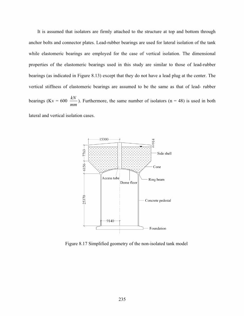
235

It is assumed that isolators are firmly attached to the structure at top and bottom through

anchor bolts and connector plates. Lead-rubber bearings are used for lateral isolation of the tank

while elastomeric bearings are employed for the case of vertical isolation. The dimensional

properties of the elastomeric bearings used in this study are similar to those of lead-rubber

bearings (as indicated in Figure 8.13) except that they do not have a lead plug at the center. The

vertical stiffness of elastomeric bearings are assumed to be the same as that of lead- rubber

bearings (Kv = 600 mm

kN). Furthermore, the same number of isolators (n = 48) is used in both

lateral and vertical isolation cases.

Figure 8.17 Simplified geometry of the non-isolated tank model

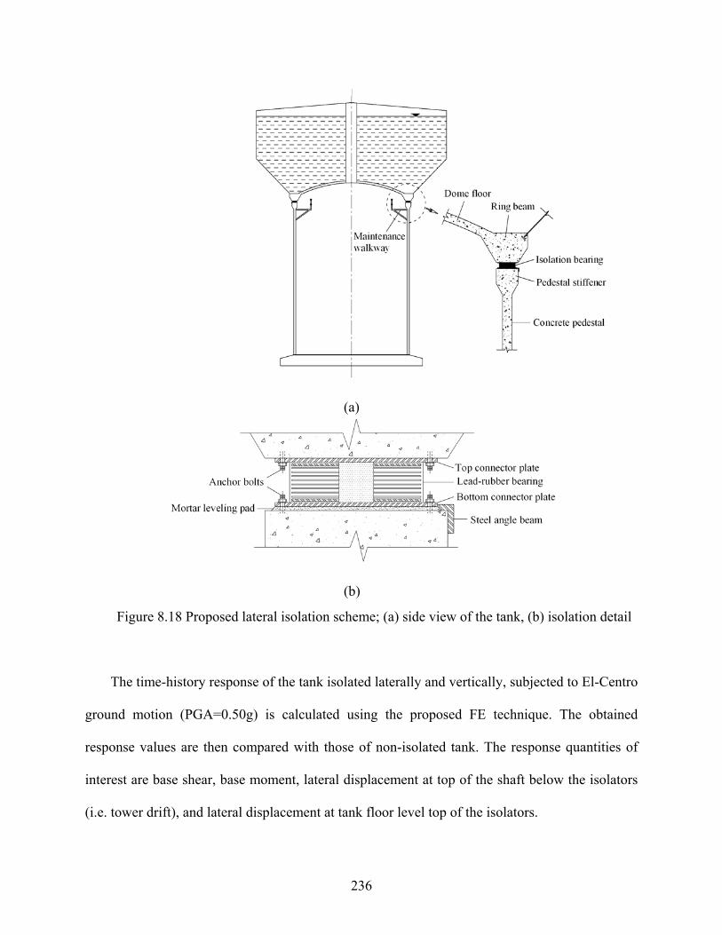
236

(a)

(b)

Figure 8.18 Proposed lateral isolation scheme; (a) side view of the tank, (b) isolation detail

The time-history response of the tank isolated laterally and vertically, subjected to El-Centro

ground motion (PGA=0.50g) is calculated using the proposed FE technique. The obtained

response values are then compared with those of non-isolated tank. The response quantities of

interest are base shear, base moment, lateral displacement at top of the shaft below the isolators

(i.e. tower drift), and lateral displacement at tank floor level top of the isolators.

237

Figure 8.19 Proposed vertical isolation scheme; (a) side view of the tank, (b) isolation detail І,

(c) isolation detail ІІ

(a)

(b)

(c)

238

Figure 8.20 shows the obtained time history responses of both laterally and vertically

isolated tanks against those corresponding to the non-isolated tank for comparison purposes.

-8.0E+04

-6.0E+04

-4.0E+04

-2.0E+04

0.0E+00

2.0E+04

4.0E+04

6.0E+04

8.0E+04

0 5 10 15 20

Time (s)

Ba

se

Sh

ea

r (k

N)

Fixed

Laterally isolated

Vertically isolated

-2.80E+06

-2.00E+06

-1.20E+06

-4.00E+05

4.00E+05

1.20E+06

2.00E+06

2.80E+06

0 5 10 15 20

Time (s) B

ase

Mo

men

t (k

Nm

)

Fixed

Laterally isolated

Vertically isolated

(a) (b)

-40

-30

-20

-10

0

10

20

30

40

0 5 10 15 20

Time (s)

To

wer

Dri

ft (

mm

)

Fixed

Laterally isolated

Vertically isolated

-80

-60

-40

-20

0

20

40

60

80

0 5 10 15 20

Time (s)

Dis

pla

cem

ent

at t

ank

flo

or

leve

l (m

m) Fixed

Laterally isolated

Vertically isolated

(c) (d)

Figure 8.20 Time-history response of the elevated tank model under El-Centro earthquake

(PGA=0.5g); (a) base shear, (b) base moment, (c) tower drift, (d) lateral displacement at tank

floor level (at top of the isolators in isolated models)

The comparisons among the response variations calculated for the fixed and isolated models

clearly show the period elongation effect in the time-history response of the isolated tank models

due to seismic isolation. Moreover, it can be observed from the figure that the base shear, base

239

moment and tower drift response values are significantly reduced due to seismic isolation in both

laterally and vertically isolated models. This verifies the effectiveness of seismic isolation in

liquid-filled conical elevated tanks. Examining the obtained results, it can be observed that in

general more reduction is achieved by the lateral isolation strategy as compared to the vertical

isolation technique. This is partly due to an additional damping effect resulting from hysteretic

energy absorption of lead-rubber bearings and partly due to the horizontal flexibility of the

bearings in laterally isolated case compared to the case of vertical isolation. However, as

indicated in Figure 8.20 (d), a different trend is observed in terms of the lateral displacement

response at tank floor level. As shown in this figure, the absolute maximum value of lateral

displacement is increased from 32.4 mm in the fixed tank case to 74.3 mm in lateral isolation

case while it is decreased to 19.4 mm in vertical isolation case. This can be the main advantage

of vertical isolation over lateral isolation strategy which offers a beneficial solution to the

difficulties which arise from the excessive deformations usually experienced in isolated

structures. This issue is especially of great importance in elevated water tanks because of the

piping system failure that may be experienced as a result of excessive deflections.

It can be concluded that when excessive deformation due to lateral isolation is not of

concern, lateral isolation strategy is usually a better option leading to a more effective solution to

the problem. On the other hand, if additional structural movements cannot be accommodated by

existing tank design, vertical isolation scheme is preferred over lateral isolation.

The absolute maximum time history response values corresponding to the isolated and non-

isolated tank models are summarized in Table 8.4. The numbers in bold show an increase

(positive) or decrease (negative) percentage over the corresponding non-isolated tank model.

240

Table 8.4 Summary of peak time history response values

Response Fixed Laterally isolated Vertically isolated

Base Shear (kN) 60251

19250 -68%

40830 -32%

Base Moment (kNm) 2326509

583244 -75%

1416708 -39%

Tower Drift (mm) 32.4

15.0

-54% 20.3

-37%

Displacement at tank floor level (mm)

32.4

74.3 +129%

19.4 -40%

For comparison purposes, the maximum response values corresponding to different isolation

schemes considered are normalized with respect to those of non-isolated tank model, as shown in

Figure 8.21.

In order to investigate the effect of seismic isolation on the sloshing response of conical

elevated tanks, the time history sloshing height is calculated for laterally isolated tank model and

is compared against that of non-isolated case, as shown in Figure 8.22.

The maximum sloshing height in the fixed base tank is 761 mm. As a result of seismic

isolation, the free-surface displacement increases by about 25% to a value of 955mm. This in

turn results in an increase in the magnitude of convective pressure by about 33% at the water free

surface. Figure 8.23 shows the total hydrodynamic pressure distribution along the height of the

tank wall for both isolated and non-isolated cases. Overall, the total hydrodynamic pressure

decreases considerably due to seismic isolation of the tank.

241

0.00

0.20

0.40

0.60

0.80

1.00B

ase

shea

r ra

tio

(V

max

/Vm

ax,F

ixed

)

1.00

0.68

0.32

Fixed Lateral isolation Ver isolation 0.00

0.20

0.40

0.60

0.80

1.00

Bas

e m

om

ent

rati

o

(Mm

ax/M

max

,Fix

ed)

1.00

0.61

0.25

Fixed Lateral isolation Ver isolation

(a) (b)

0.00

0.20

0.40

0.60

0.80

1.00

To

wer

dri

ft r

atio

(U

max

/Um

ax,F

ixed

)

1.00

0.63

0.46

Fixed Lateral isolation Ver isolation0.00

0.50

1.00

1.50

2.00

2.50

Tan

k fl

oo

r d

isp

lace

men

t ra

tio

(X

max

/Xm

ax,F

ixed

)

1.00

0.60

2.29

Fixed Lateral isolation Ver isolation

(c) (d)

Figure 8.21 Normalized peak time history response values; (a) base shear, (b) base moment,

(c) tower drift, (d) displacement at tank floor level

-1200

-900

-600

-300

0

300

600

900

1200

0 5 10 15 20

Time (s)

Slo

sh

ing

Dis

pla

ce

men

t (m

m)

Laterally isolated

Fixed

Figure 8.22 Time history of sloshing height at water free surface

242

-13

-11

-9

-7

-5

-3

-1

0 30 60 90 120 150

Total hydrodynamic pressure (kPa)

Wat

er

de

pth

(m

)

Laterally isolated

Fixed


Water depth = -6.85 m

Figure 8.23 Hydrodynamic pressure distribution over the tank wall

The maximum total hydrodynamic pressure reduces by about 80% due to lateral seismic

isolation. A similar trend was observed in the experimental study carried out by Chalhoub and

Kelly (1990) on cylindrical ground-supported water tanks. Malhotra (1997C) and Shekari et al.

(2009) also found a similar trend in response for cylindrical ground-supported tanks isolated by

rubber bearings. This could be interpreted as a stronger coupling observed between the longer

period dominant isolation mode and the fundamental convective mode in the isolated tank case

in comparison to the totally uncoupled (well-separated natural periods) fundamental impulsive

and convective modes usually observed in typical fixed base tanks. As will be discussed later in

this chapter, this long-period content isolation mode together with the fundamental convective

mode characterize the motion of isolated elevated tanks. Nonetheless, the observed increase in

sloshing response due to isolation of the tank is negligible and can be overcome by the proper

choice of the isolation design and/or by the installation of dampers at the location of peak free-

surface sloshing.

243

The reduction in total hydrodynamic pressure due to seismic isolation can be considered as

another measure of the effectiveness of the seismic isolation system.

The magnitude of the impulsive component of pressure is mainly dependent on the absolute

acceleration of the impulsive water mass. As a result of seismic isolation, this acceleration is

reduced significantly leading to a considerable reduction in the magnitude of impulsive pressure.

This reduction in impulsive pressure offsets the increase in convective pressure due to seismic

isolation which thus results in a significant net decrease in the total hydrodynamic pressure, as

shown in Figure 8.23.

8.3.5.3 Effect of isolation location on response

To consider the effect of isolators’ location on the dynamic response of conical elevated

tanks, the considered tank model is laterally isolated using two different isolation schemes as

follows:

1) Isolation type A in which isolators are located at the base of the shaft as shown in Figure

8.24 (a).

2) Isolation type B in which isolators are provided at top of the shaft immediately below the

concrete ring beam as shown in Figure 8.24(b).

The elevated tank model considered for this part of study is the same as that used in the

previous section. Figure 8.17 shows the geometrical properties of the corresponding non-isolated

tank model.

244

(a) (b)

Figure 8.24 Schematic geometries of the isolated tank models; (a) Isolation type A,

(b) Isolation type B

Figure 8.25 shows the time history variation of response of the elevated tank model in fixed

and isolated conditions considering the two locations for seismic isolators. As obvious from the

figure, different response variations are obtained for isolation types A and B.

The absolute maximum time history response values corresponding to the isolated and non-

isolated tank models are summarized in Table 8.5. The numbers in bold show an increase


For comparison purposes, the maximum response values corresponding to different isolation

types considered are normalized with respect to those of non-isolated tank model, as shown in

Figure 8.26.

245

-8.0E+04

-6.0E+04

-4.0E+04

-2.0E+04

0.0E+00

2.0E+04

4.0E+04

6.0E+04

8.0E+04

0 5 10 15 20

Time (s)

Bas

e S

hea

r (k

N)

Isolation type A

Isolation type B

Fixed

-2.8E+06

-2.0E+06

-1.2E+06

-4.0E+05

4.0E+05

1.2E+06

2.0E+06

2.8E+06

0 5 10 15 20

Time (s)

Bas

e M

om

ent

(kN

m)

Isolation type A

Isolation type B

Fixed

(a) (b)

-40

-30

-20

-10

0

10

20

30

40

0 5 10 15 20

Time (s)

To

wer

Dri

ft (

mm

)

Isolation type A

Isolation type B

Fixed

-100

-80

-60

-40

-20

0

20

40

60

80

100

0 5 10 15 20

Time (s)

Dis

pla

cem

ent

at t

ank

flo

or

leve

l (m

m)

Isolation type A

Isolation type B

Fixed

(c) (d)

-80

-60

-40

-20

0

20

40

60

80

0 5 10 15 20

Time (s)

Bea

rin

g D

isp

lace

men

t (m

m)

Isolation type A

Isolation type B

(e)

Figure 8.25 Time-history response of the elevated tank models considering different

locations for isolators; (a) base shear, (b) base moment, (c) tower drift, (d) lateral displacement at

tank floor level, (e) bearing displacement

246

Table 8.5 Peak time history response values considering different locations for isolators

Response * Fixed Isolation type B Isolation type A

Base Shear (kN) 60251 19250 -68%

16278 -73%

Base Moment (kNm) 2326509 583244 -75%

515243 -78%

Tower Drift (mm) 32.4 15.0

-54% 21.2

-35%

Displacement at tank floor level (mm)

32.4 74.3

+129% 88.3

+173%

* All response values given in the table are maximum absolute values.

0.00

0.20

0.40

0.60

0.80

1.00

Ba

se

sh

ea

r ra

tio

(V

ma

x/V

ma

x,F

ixe

d)

1.00

0.270.32

Fixed Isolation type B Isolation type A0.00

0.20

0.40

0.60

0.80

1.00

Ba

se

mo

me

nt

rati

o

(Mm

ax

/Mm

ax

,Fix

ed

)1.00

0.220.25

Fixed Isolation type B Isolation type A

(a) (b)

0.00

0.20

0.40

0.60

0.80

1.00

To

we

r d

rift

ra

tio

(U

ma

x/U

ma

x,F

ixe

d)

1.00

0.65

0.46

Fixed Isolation type B Isolation type A0.00

0.50

1.00

1.50

2.00

2.50

3.00

Ta

nk

flo

or

dis

pla

ce

me

nt

rati

o

(Xm

ax

/Xm

ax

,Fix

ed

)

1.00

2.73

2.29

Fixed Isolation type B Isolation type A

(c) (d)

Figure 8.26 Normalized peak time history response values considering different locations

for seismic isolators; (a) base shear, (b) base moment, (c) tower drift, (d) displacement at tank

floor level

247

As presented in Table 8.5, in both isolation types, the values of base shear and base moment

are reduced significantly. However, generally, more reduction is achieved by isolation type A as

compared to isolation type B. A different trend is observed for tower drift response. Isolation

type B results in a reduction percentage of around 54% in tower drift response value while only

35% reduction is achieved by isolation type A. In terms of displacement at tank floor level,

isolation type B is considered more advantageous over isolation type A, as less increase

percentage is observed in isolation type B (129%) in comparison to the increase percentage of

173% calculated for isolation type A.

The maximum absolute bearing displacements calculated for isolation types A and B are 68

mm and 60 mm, respectively. This indicates that the bearing displacement is slightly smaller in

the tank with isolation type B in comparison to the isolation type A since the weight applied on

isolation type B is comparatively less than that in isolation type A. This is obvious in Figure 8.27

which shows the force-displacement hysteretic loops during the considered earthquake motion

corresponding to isolation types A and B. The given hysteretic diagram is for one isolator. The

enclosed area in a force-displacement hysteretic loop implies the energy dissipated in a cycle.

According to the calculated hysteretic loops indicated in this figure, one can notice that the

total amount of energy absorbed during the earthquake increases when isolators are located at the

base of the tank compared to the case where bearings are installed at top of the shaft. This could

be considered as another advantage for isolation type A over isolation type B. The reason is

believed to be the increase in vertical loads applied to the isolators due to the self weight of the

shaft, weight of platforms inside the shaft and their live load, and the weights of all other

accessories attached to the shaft structure. This phenomenon has also been noticed

experimentally in research works by Robinson (1982) and King (1980).

248

-375

-250

-125

0

125

250

375

-75 -50 -25 0 25 50 75

Displacement (mm)

Fo

rce

(k

N)

Isolation type A

Isolation type B

Figure 8.27 Force-displacement diagram for seismic isolation types A and B

8.3.5.4 Effect of stiffness of the shaft structure (natural period of the shaft structure)

To study the effect of shaft stiffness on the effectiveness of seismic isolation, two elevated

tank models having different shaft stiffness characteristics namely; stiff and flexible are

considered and their time history response is calculated using the proposed methodology.

The two tanks are assumed to be laterally isolated at top of the shaft structure and the same

isolation properties are considered for both stiff and flexible models. The properties of the

considered isolation system are as explained before under section 8.3.5.1. The elevated tank

model considered for this part of study is the same as that used in the previous section. See

Figure 8.17 for the geometrical properties of the corresponding tank model. The flexible tank

model is created by reducing the shaft thickness to 127 mm such that the resulting shaft stiffness

reaches as low as one third of that of the original model (stiff model). As mentioned before, the

249

thickness of the shaft structure in the original model (stiff model) is 380 mm. All other properties

of the two tank models are assumed to be the same.

Table 8.6 lists the peak time history response values of the isolated stiff and flexible tank

models against corresponding non-isolated tanks. The numbers in bold show an increase


Table 8.6 Peak time history response values for stiff and flexible tank models

Original shaft stiffness

(Stiff model) Low shaft stiffness (Flexible model)

Response * Fixed Isolated Fixed Isolated

Base Shear (kN)

60251 19250 -68%

35182 16156 -54%

Base Moment (kNm)

2326509 583244 -75%

1266423 518286 -59%

Tower Drift (mm)

32.4 15.0

-54% 59.5

45.3 -24%

* All response values given in the table are maximum absolute values.

Table 8.6 shows that for stiff model, the reduction percentages in base shear, base moment,

and tower drift, as a result of isolation, are 68%, 75%, and 54%, respectively, while the

corresponding reductions for flexible model are 54%, 59%, and 24%. The obtained results show

a considerable reduction in dynamic response of the tanks due to seismic isolation in both stiff

and flexible cases. However, this reduction is comparatively more pronounced in stiff model in

comparison to flexible model. As a result, it can be concluded that seismic isolation is

comparatively more effective in tanks with stiffer shaft structure compared to those having more

flexible shaft structures given that all other properties are the same.

250

Comparing the results obtained for non-isolated stiff and flexible tanks, it can be noticed that

smaller seismic forces are transmitted by the flexible shaft structure resulting in smaller base

shear and base moment response values. However, this flexibility has resulted in an increase of

around 84% in tower drift.

The peak base shear and base moment response values calculated for the isolated tanks are

compared against those of non-isolated tanks for two different values of shaft stiffness, as

indicated in Figure 8.28.

0.0E+00

1.0E+04

2.0E+04

3.0E+04

4.0E+04

5.0E+04

6.0E+04

7.0E+04

Ba

se

Sh

ea

r (k

N)

Fixed

Isolated

Stiff Flexible 0.0E+00

5.0E+05

1.0E+06

1.5E+06

2.0E+06

2.5E+06

Bas

e M

om

en

t (k

Nm

)

Fixed

Isolated

Stiff Flexible

(a) (b)

Figure 8.28 Comparison of results between stiff and flexible tank models

As obvious from the figure, the response of isolated tanks is obviously less sensitive to the

flexibility of the shaft structure as compared to the corresponding non-isolated tanks. In other

words, the dynamic response of isolated tanks is not significantly influenced by the stiffness

properties of the supporting shaft structure.

8.3.5.5 Effect of tank aspect ratio

In order to investigate the sensitivity of seismic isolation to the tank’s geometry, the

transient response of two elevated tank models having different aspect ratios namely; broad and

251

slender is determined in both isolated and non-isolated conditions using the proposed FE scheme.

The effectiveness of seismic isolation is then examined by comparing the results obtained for

broad and slender configurations.

The considered broad and slender tank models have the aspect ratios of 0.7 and 2.1,

respectively. Tank aspect ratio (A.R.) is defined as the ratio of equivalent water height (based on

the concept of equivalent cylinder model) to the radius of the cylindrical part of the vessel.

The broad tank model considered in this section is the same as that used in Chapter 6,

section 6.2.3 and elsewhere throughout this chapter (see Figure 8.17). The simplified geometries

of the tanks along with their FE models are indicated in Figure 8.29.

The tanks are assumed to be laterally isolated at top of the shaft structure, and the same

isolation properties are considered for both broad and slender models. The properties of the

considered isolation system are as explained before under section 8.3.5.1.

The volume of contained water is the same in both cases. Furthermore, the stiffness and

mass distributions along the height of the shaft, and conical and cylindrical side shells are similar

in both tank models. The mass distributions are made equivalent by adjusting the mass density of

each section (shaft, cone, and cylinder parts) of the tank appropriately. As a result of this

adjustment, the total mass of broad and slender tank models will also be the same.

The stiffness distributions are also made equivalent by altering the thickness of each shell

section (shaft, cone, and cylinder parts) of the tank properly such that the resulting stiffness

matches that of broad tank model. These adjustments result in equal values of shaft period,

isolation time period, and isolation yield strength in broad and slender tank models. Thus, the

obtained time history results are readily comparable.

252

(a)

(b)

Figure 8.29 Broad and slender tank models; (a) simplified geometries, (b) FE models

253

Table 8.7 lists the peak time history response values of the isolated broad and slender tank

models against corresponding non-isolated tanks. The numbers in bold show an increase


As presented in the table, the base shear and base moment values of slender tank model are

greater than those of broad tank in both fixed and isolated conditions. This reveals the significant

effect of tank’s geometry on the dynamic response of the elevated tanks in both fixed and

isolated conditions.

Table 8.7 shows that for broad model, the reduction percentages in base shear, base moment,

and tower drift, as a result of isolation, are 68%, 75%, and 54%, respectively, while the

corresponding reductions for slender model are 77%, 79%, and 78%. Therefore, it can be

concluded that comparatively greater reductions in dynamic response can be achieved due to

seismic isolation in slender tank as compared to broad tank.

Table 8.7 Peak time history response values for broad and slender tank models

Tank model Bearing Disp.

(mm) * Sloshing Disp.

(mm) Base Shear

(kN) * Base Moment

(kNm) * Tower Drift

(mm) *

Broad Fixed NA 761 60251 2326509 32.4

Isolated 60 955

+25% 19250 -68%

583244 -75%

15.0 -54%

Slender Fixed NA 844 88810 3211956 36.9

Isolated 83 1148

+36% 20785 -77%

690779 -79%

8.2 -78 %

* Values given for these response quantities are maximum absolute values.

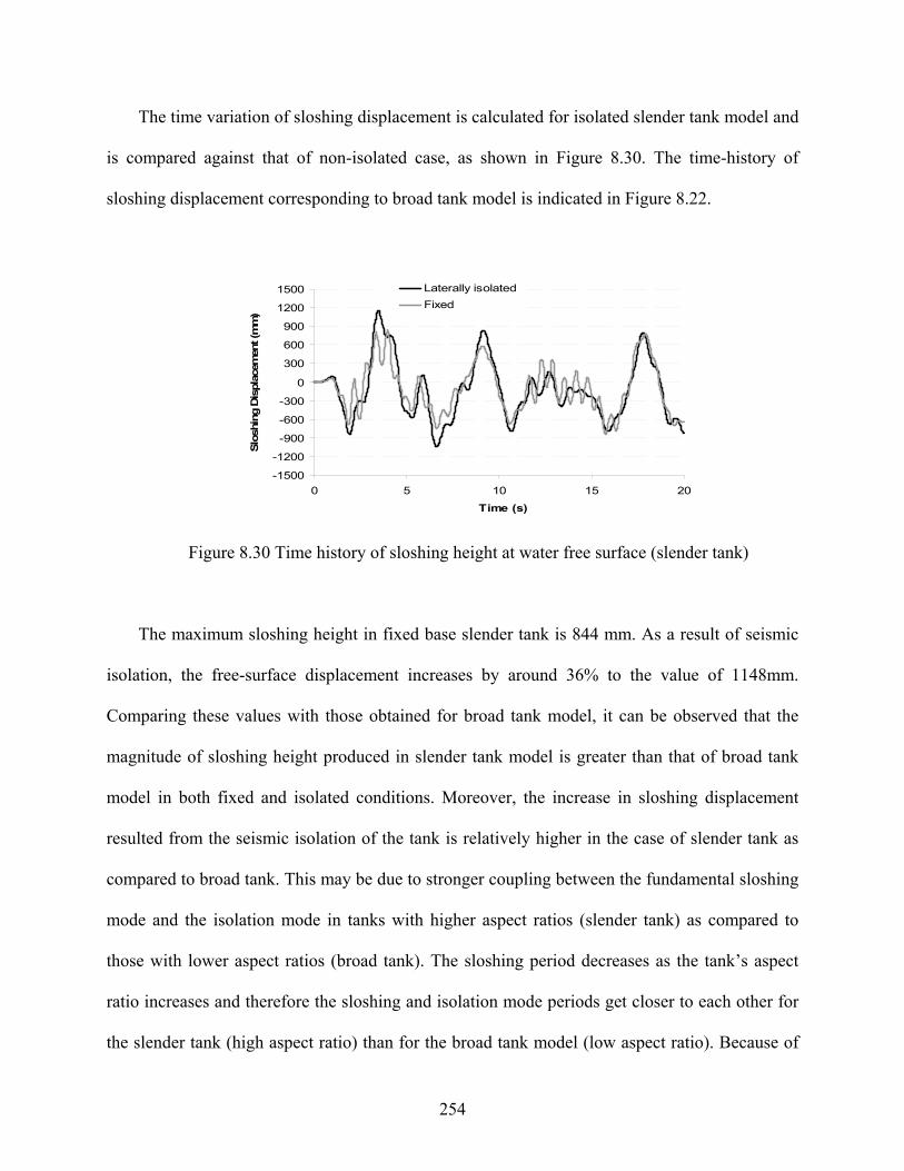
254

The time variation of sloshing displacement is calculated for isolated slender tank model and

is compared against that of non-isolated case, as shown in Figure 8.30. The time-history of

sloshing displacement corresponding to broad tank model is indicated in Figure 8.22.

-1500

-1200

-900

-600

-300

0

300

600

900

1200

1500

0 5 10 15 20

Time (s)

Slo

shin

g D

ispla

cem

ent (m

m)

Laterally isolated

Fixed

Figure 8.30 Time history of sloshing height at water free surface (slender tank)

The maximum sloshing height in fixed base slender tank is 844 mm. As a result of seismic

isolation, the free-surface displacement increases by around 36% to the value of 1148mm.

Comparing these values with those obtained for broad tank model, it can be observed that the

magnitude of sloshing height produced in slender tank model is greater than that of broad tank

model in both fixed and isolated conditions. Moreover, the increase in sloshing displacement

resulted from the seismic isolation of the tank is relatively higher in the case of slender tank as

compared to broad tank. This may be due to stronger coupling between the fundamental sloshing

mode and the isolation mode in tanks with higher aspect ratios (slender tank) as compared to

those with lower aspect ratios (broad tank). The sloshing period decreases as the tank’s aspect

ratio increases and therefore the sloshing and isolation mode periods get closer to each other for

the slender tank (high aspect ratio) than for the broad tank model (low aspect ratio). Because of

255

the possible interaction between the sloshing and isolation modes of vibration, especially in

slender tanks, the contributions of both modes should be considered for an accurate analysis of

isolated elevated tank models. Therefore, a single mode solution (based on the “isolation mode”

only) recommended for most of the isolated systems (such as in buildings) is not adequate to

accurately estimate the seismic response of isolated elevated tanks.

The maximum absolute bearing displacements for broad and slender tank models are 60 mm

and 83 mm, respectively. This reveals that bearing displacement is relatively smaller in broad

tank as compared to slender tank or in other words, the bearing displacement increases as the

aspect ratio increases.

Figure 8.31 shows the force-displacement hysteretic loops during the earthquake

corresponding to broad and slender tank models. As obvious from this figure, the total amount of

absorbed energy increases as the tank’s aspect ratio increases. This could be considered as

another advantage for slender tanks over broad tanks in seismic isolation applications.

-375

-250

-125

0

125

250

375

-100 -75 -50 -25 0 25 50 75 100

Displacement (mm)

Fo

rce

(kN

)

Slender Tank

Broad Tank

A

Figure 8.31 Force-displacement diagram for broad and slender tank models

256

Overall, comparing the total amount of absorbed energy between two cases, and also the

reduction percentages achieved in the considered response quantities through seismic isolation, it

can be concluded that seismic isolation is comparatively more effective in slender tanks in

comparison to broad tanks.

8.3.5.6 Effect of yield strength of isolators

In this section, the influence of the yield strength of bearings on seismic response of isolated

conical elevated tanks is investigated. The elevated tank model considered for this part of study

is the same as that used in sections 8.3.5.2 to 8.3.5.4 of this chapter. See Figure 8.17 for the

geometrical properties of the corresponding non-isolated tank model. Furthermore, the

considered tank models are assumed to be laterally isolated at top of the shaft structure.

Figure 8.32 shows the variation of normalized base shear (Vmax/W) versus normalized

yield strength of isolators (Qy/W), where, W is the weight supported by the bearings. In

obtaining this graph, five different isolation systems having different yield strength ratios

(Qy/W) are considered. All other properties of the considered isolation systems are the same.

The tank models analyzed previously had the Qy/W ratio of 0.125.

The Figure initially shows a decreasing trend in the base shear as the yield strength ratio

increases up to about 5% at which the minimum base shear is attained. Beyond this point, any

further increase in yield strength ratio result in increase in base shear ratio. As a result, it can be

said that there is an optimum value for the yield strength of isolators leading to a minimum value

of the seismic response. For the specific tank and earthquake record considered in this study, this

optimum value is found to be about 5% of the weight carried by isolators.

257

0.00

0.05

0.10

0.15

0.20

0.25

0.025 0.050 0.075 0.100 0.125

Qy/W

Vm

ax/W

Optimum point

Figure 8.32 Effect of the yield strength of isolators on the dynamic response of

elevated tank model

A proper choice of the yield strength of isolators plays an important role in achieving the

minimum dynamic response in isolated elevated tanks. However, attention should be drawn to

the fact that any decrease in the yield strength of bearings will result in an increase in the bearing

displacement which might not be desirable based on the specific design requirements for both the

tank and the bearings. Therefore, in selecting the appropriate properties of the isolation system,

both the seismic forces transmitted to the structure and the displacement to be accommodated by

the bearings should be taken into account.

8.3.5.7 Free vibration analysis of isolated elevated tanks

Free-vibration analysis is performed on an isolated elevated tank model in order to

investigate the properties of the modes having major contributions to the response. The tank

model considered for this part of study is shown in Figure 8.17. The tank is assumed to be

laterally isolated at the base. The properties of the considered isolation system are as explained

previously under section 8.3.5.1.

258

Table 8.8 lists natural frequencies for the convective, impulsive, and base-isolation modes of

the isolated tank model as well as those of non-isolated tank. In addition, the modal participation

factors (β) normalized with respect to their largest values for each model are also given in the

table.

As given in the table, the period of the isolated tank model (1.65 sec) is several times longer

than the impulsive period of the corresponding non-isolated model (0.51 sec). In an effective

isolation design, the period of the isolation mode should be greater than the period of the

fundamental impulsive mode in the corresponding fixed-base tank model. However, this

extended period should not be in close vicinity to the fundamental sloshing period as this may

cause an excessive increase in sloshing height due to resonance effect. This is not expected to

occur since the sloshing period is usually very large.

Generally, seismic isolation systems should be designed in such a way that their dominant

frequency be in the range of 0.25 to 1.00 Hz (Kim and Lee (1995)). This range is referred to as

the effective frequency range resulting in an effective seismic isolation of the structure. As

shown in Table 8.8, the natural frequency of the base-isolation mode (0.606 Hz) for the tank

model under consideration is in the effective frequency range for seismic isolation systems.

Furthermore, it can be observed from the table that the natural frequency corresponding to the

impulsive mode has been shifted from 1.955 Hz to a higher value of 3.095 Hz as a result of base

isolation. However, no frequency shift is observed in convective modes indicating that base

isolation has no significant effect on sloshing modes. This phenomenon reveals that impulsive

modes are more significantly influenced by the properties of seismic isolation system as

compared to convective modes.

259

Table 8.8 Comparison of free-vibration analysis results between fixed-base and base-

isolated elevated tank models

Fixed-base model Base-isolated model

Mode type Frequency, Hz (Period, sec)

β (normalized) Frequency, Hz (Period, sec)

β (normalized)

Convective 0.161 (6.21) 1.00 0.157 (6.37) 0.74

Impulsive 1.955 (0.51) 0.88 3.095 (0.32) 0.05

Base-isolation NA NA 0.606 (1.65) 1.00

Figure 8.33 shows normalized modal participation factors (β) for the base-isolated tank

model. As shown in the figure, the modal participation factor of the base-isolation mode is

largest implying that this mode dominates the total dynamic response of the base-isolated tank

model. Convective mode has the second highest modal participation factor among all modes of

vibration. The participation factor corresponding to the impulsive mode is very small compared

to the other modes suggesting that this mode does not contribute significantly in the overall

seismic response of the model. As a result, to accurately capture the dynamic response of

isolated elevated tanks, the contributions of both isolation and convective modes of vibration

should be taken into account.

Similar to fixed-base tank models, convective mode in isolated elevated tanks is associated

with the fluid motion at the tank’s free surface. No significant motion is observed in the shaft,

tank shell, and isolation system in the convective mode. The isolation mode is associated with a

large displacement in the isolation system and very small tower drift amplitude. This is typically

referred to as a rigid body motion. The obtained impulsive mode shape indicates considerable

deflections in the shaft, tank shell, and isolation system.

260

0.00

0.20

0.40

0.60

0.80

1.00

No

rma

lize

d M

od

al

Pa

rtic

ipa

tio

n F

ac

tor

Convective Mode

Impulsive Mode

Base Isolation Mode

0.74

1.00

0.05

Figure 8.33 Normalized modal participation factors (β) for the base-isolated tank model

8.4 Summary

In the first part of this chapter, a detailed finite element method was employed to study the

fluid-structure interaction for liquid-filled conical elevated tanks with varying cone angles.

Transient analyses using modal superposition technique were carried out to investigate the effect

of cone slope angle on the base shear and base moment response of the supporting structure in

elevated water tanks. Effects of tank wall flexibility, water sloshing and the rocking component

as well as the lateral translational component were taken into consideration in the proposed FE

analysis. Different damping ratios corresponding to the different parts of response (impulsive

and convective) were assigned to the model. In addition, the instantaneous values of the sloshing

and impulsive terms were determined separately.

Free vibration FE analyses resulted in natural frequencies and effective water mass ratios

very close to those obtained from Housner's formulations with differences for water mass ratios

smaller than 5% of the total mass of the fluid for all cases considered.

The sloshing response of the elevated water tanks considered was mainly dominated with

the fundamental sloshing mode. However the results showed that the impulsive response of the

tank models having large cone angles could not be accurately predicted by only considering the

261

fundamental impulsive mode. As a result, more impulsive modes other than the fundamental

impulsive mode are needed in studying the dynamic behavior of such models.

Time history analyses of the elevated water tanks with different geometries showed that the

effect of cone angle variations could be significant on the impulsive component of the response

but not on the convective part. Increasing the cone angle and thereby increasing the unsupported

cantilever length of the tank floor resulted in new dominant rocking modes having high

participation factors and effective mass ratios. These rocking modes characterized with their

relatively small natural frequencies had smaller associated response spectrum accelerations

compared to those of typical lateral translational impulsive modes. Therefore, smaller shear

forces and overturning moments were exerted at the shaft base of the elevated tanks having large

cone angles (namely models C, D, and E in the current study). For instance, by only increasing

the cone angle from 45° to 75°, the base shear and base moment of the shaft structure were

decreased by a factor of 2.3 and 3.0, respectively. This allows much slimmer and lighter design

of all supporting structures, including the shaft structure and the foundation system.

The computed FE time history results were also compared with those obtained from current

practice. The current practice provided reasonable estimations for models with translational

dominant behavior. However, the results were too conservative for models having dominant

rocking behavior leading to an overdesign of the structure. As a result, it is recommended that a

dynamic model having the capability to consider both lateral translational and rotational degrees

of freedom be employed for the analysis of such structures.

In the second part of this chapter, some important aspects on elastomeric and lead-rubber

bearings, their elaborate FE modeling, and their force-displacement behavior were addressed.

Using the proposed FE technique, modeling of the nonlinear behavior of rubber material was

262

made possible. Optimum rubber material parameters were estimated successfully using a robust

parameter identification scheme from several available experimental data simultaneously. The

obtained set of material parameters resulted in an excellent correlation between experimental and

analytical results under different deformation states and from low to high strain levels.

The load-deformation response of two typical full-scale lead-rubber bearings under the

combined action of compression and shear was obtained up to moderate strain levels using the

proposed FE procedure. The calculated FE results correlated well with those of the experimental

study ensuring the adequacy of the proposed FE model. Employing this numerical model can

result in a significant reduction in the amount of experimental and/or analytical work required to

accurately characterize the hysteretic behavior of this type of isolators. Moreover, this elaborate

FE model can be used to determine the global parameters of the simplified two-node model

proposed for the practical simulation of the seismic behavior of rubber bearings in this study.

It was observed that the proposed simplified model was capable of accurately estimating the

hysteretic response of energy dissipation devices with less computational efforts. The proposed

simplified modeling approach is practical, accurate enough, and easy to use in 3D FE

applications.

In the last part of this chapter, an attempt was made to apply seismic isolation using lead-

rubber and elastomeric bearings to liquid-filled conical elevated tanks.

To investigate the effectiveness of seismic isolation for this type of structures, the dynamic

response of both fixed and isolated conical elevated tanks partially filled with water was

investigated using a three-dimensional numerical procedure under horizontal seismic excitations.

Various studies were carried out to investigate the effects of different parameters on the

effectiveness of the seismic isolation system. The examined parameters included: lateral versus

263

vertical isolation, different locations of isolators, shaft stiffness, tank aspect ratio, and yield

strength of isolators.

Two possible construction details for vertical isolation and one detail for lateral isolation of

conical elevated tanks were considered. It was observed that the application of passive control

devices to conical elevated water tanks could offer a substantial benefit for the earthquake-

resistant design of such structures. The magnitude and distribution of seismically induced forces,

moments and displacements could be controlled through appropriate selection of device

properties, isolators’ locations, and tank’s structural and geometrical characteristics.

The results of this study show the effectiveness of seismic isolation technique for these types

of structures. In general, it can be concluded that the magnitude of tower drift, total

hydrodynamic pressure, and seismically induced forces and moments is reduced significantly

due to the presence of seismic isolation system whose dominant frequency is within the effective

frequency range of seismically isolated systems. However, an increase in displacements in

laterally isolated tanks seems to be inevitable unless providing additional damping is considered.

The extra cost imposed by installing seismic isolators is expected to be offset by the additional

savings achieved due to seismic isolation in the shaft structure, foundation and anchorage

system, and tank material.

In general it was observed that more reduction in seismic shear, moment, and tower drift

was achieved due to the lateral isolation scheme as compared to the vertical isolation. However,

a different trend in response was observed in terms of lateral displacement at tank floor level.

Vertical isolation resulted in a considerable reduction in lateral displacement while a significant

increase in lateral displacement was experienced in the laterally isolated tank model. This could

be the main advantage of vertical isolation over lateral isolation system. As a result, it can be

264

concluded that when excessive deformation due to lateral isolation is not of concern, this

isolation strategy is usually a better option leading to a more effective solution to the problem.

On the other hand, if additional structural movements can not be accommodated by existing tank

design, vertical isolation scheme is preferred over lateral isolation.

Despite the foregoing advantages, it was observed that the sloshing height was amplified

due to seismic isolation of the tanks in both broad and slender tank configurations. However, a

greater amplification in sloshing displacement was noticed in the case of slender tank as

compared to broad tank. This may be considered as a drawback for the isolated elevated tank

systems as compared to the typical fixed-base tanks. It was also observed that the contribution of

convective pressure component was negligibly increased as a result of seismic isolation, however

the total hydrodynamic pressure was reduced significantly.

To determine the optimum location of seismic isolators for elevated water tanks, two

different isolated models (isolation type A and B) were selected and base shear, base moment,

tower drift, lateral displacement at tank floor level, bearing displacement, and absorbed energy

were examined under the horizontal component of 1940 El-Centro record. In isolation type A,

isolators were located at the base of the tank while in isolation type B, isolators were provided at

top of the shaft structure immediately below the concrete ring beam. Isolation types A and B

predicted different response variations. More reduction in base shear and base moment response

values was achieved by isolation type A as compared to isolation type B. However, a different

trend was noticed for tower drift response. In terms of displacement at tank floor level, isolation

type B was found to be more advantageous over isolation type A. In addition, a slightly smaller

bearing displacement was obtained for isolation type B as compared to isolation type A. In

addition, the amount of energy dissipated during the seismic excitation was increased where

265

isolators were located at the base of the tank compared to the case where isolators were placed at

top of the shaft structure.

Higher isolation efficiency was observed in tanks having stiffer shaft structure in

comparison to those with more flexible shaft structure. It was shown that the seismic response of

isolated tanks was not considerably affected by the flexibility of the shaft structure.

The seismic isolation resulted in significant advantages for both broad and slender tank

configurations. However, slender tanks were found to be better candidates in terms of more

effective application of seismic isolation. Sloshing displacement in slender tank was

comparatively greater than that of broad tank in both isolated and non-isolated conditions.

Due to a potential coupling between the sloshing and isolation modes of vibration,

especially in slender tanks, an accurate estimation of seismic response of isolated elevated tanks

is achievable by considering the contributions of at least two modes of vibration; convective

mode and isolation mode. It was also observed that the bearing displacement increased as the

tank’s aspect ratio increased resulting in an increase in the total amount of absorbed energy.

The results of the study also revealed that there was an optimum value for the yield strength

of isolators at which the seismic response (base shear) of the tank reached its minimum value.

For the specific tank and seismic excitation used in this study, this optimum value was

determined to be about 5% of the weight applied on the isolators.

Based on the results of free-vibration analysis performed on a base-isolated elevated tank

model, it was observed that impulsive modes were significantly affected by the properties of

seismic isolation system in comparison to sloshing modes. Based on the calculated modal

participation factors, it can be concluded that the base-isolation mode dominates the total

dynamic response of the base-isolated tank model. The second highest modal participation factor

266

among all modes of vibration was found for the convective mode. The participation factor

corresponding to the impulsive mode was found to be very small implying that this mode does

not contribute considerably in the overall seismic response of isolated elevated tanks.

267

CHAPTER 9

SUMMARY, CONCLUSIONS AND RECOMMENDATIONS

9.1 Summary

The main focus of the current study was to evaluate the performance of cylindrical ground-

supported as well as conical elevated water tanks under seismic excitations using a rigorous and

efficient finite element technique.

As a result of major advances in computer science and the development of rigorous

numerical codes, academic and industrial interest in the use of finite element technique as a tool

to investigate the fluid-structure interaction problems has greatly increased in recent years. Using

this technique, more precise and realistic results are generally obtainable. In this research study,

the fluid-structure coupling formulations were solved using a finite element technique. Various

kinds of analysis including modal, spectral and time history analysis using both modal

superposition and direct integration methods were carried out using the general-purpose finite

element analysis program ANSYS®. Throughout this study, the effects of important factors on

dynamic behavior of such structures were addressed. The examined parameters were sloshing of

liquid free surface, tank wall flexibility, vertical ground acceleration, tank aspect ratio, base

fixity, and higher impulsive and convective modes.

The accuracy of the proposed numerical model was verified by comparing the obtained

results with other analytical and experimental results available in the literature.

According to the methodology commonly used in current design standards, the dynamic

response of partially filled liquid tanks is calculated using simplified mechanical models and a

frequency-based approach. The Housner’s method is the most well-known procedure employed

268

in current design practice for seismic analysis and design of liquid tanks. In this technique, the

tank hydrodynamic response is divided into two components; "impulsive" and “convective”. In

order to investigate the validity of current code provisions in seismic analysis and design of

liquid containing structures, the obtained FE results were compared with those recommended by

current practice and important conclusions were drawn.

Furthermore, the effect of earthquake frequency content on the seismic behavior of liquid-

filled elevated tanks was investigated. To do so, a typical elevated tank model was numerically

simulated using FEM in a three-dimensional space and its seismic response was determined

under the effect of different seismic excitations having different frequency content

characteristics.

The seismic behavior of elevated water tanks was further studied by carrying out a

comprehensive parametric study on liquid-filled conical elevated tanks using the finite element

technique. Through this parametric study, a broad range of tank capacities and geometries

typically found in use today was covered. This parametric study led to generation of pressure

distribution graphs corresponding to both impulsive and convective components for a large

number of conical elevated tanks having different geometrical properties. It was also indicated

that the proposed pressure graphs could be employed simply in design applications for liquid-

filled conical elevated tanks.

The applicability of two different menshin techniques to liquid-filled conical elevated tanks

was investigated. As a first menshin technique, “Natural period adjustment method” was

introduced and its effectiveness was investigated using a rigorous finite element method in a

three-dimensional space. In this technique, the natural period of the elevated tank model was

extended far beyond the predominant period of the input seismic motion by making alterations in

269

tank’s configuration/geometry. This was achieved by increasing the inclined cone angle of the

lower portion of the vessel. As a second menshin technique, the application of seismic isolation

method to conical elevated tanks was examined. In this technique, the shaft structure was

isolated either at top immediately below the ring beam level or at the base by means of

elastomeric and lead-rubber bearings.

9.2 Conclusions

Based on the results of this research study, the following conclusions are made regarding the

dynamic behavior of ground-supported cylindrical containers:

1. The proposed FE procedure can be accurately employed in dynamic analysis of liquid

containers. Using this method, all aspects in fluid-structure interaction problems can be

considered including wall flexibility, sloshing motion, damping properties of fluid

domain, and the individual effects of impulsive and convective terms in a three-

dimensional space.

2. For practical purposes, only the fundamental impulsive and convective modes are

sufficient for characterizing the dynamic response of ground-supported cylindrical tanks

to horizontal excitations. Moreover, the cos(nθ) type modes (n > 1) have a negligible

effect on the overall dynamic response of the tanks to horizontal excitations. Modes

having the highest contributions to the response are cantilever beam type modes with n =

1.

3. Since the sloshing and impulsive components of the response do not reach their peak

values at the same time, the effect of considering sloshing term on the total response

might be either increasing or decreasing.

270

4. The effect of convective term on the overall dynamic response of cylindrical ground-

supported containers is rather more significant in shallow tanks compared to tall tanks.

5. Including the wall flexibility result in a significant increase on the impulsive component

of response. However, the convective component of response is found to be almost

independent of the tank wall flexibility. Furthermore, the sloshing height of the liquid

inside the tanks is not significantly affected by the wall flexibility.

6. Considering the combined effect of horizontal and vertical excitations, it is concluded

that including the vertical acceleration effect leads to an increase in both impulsive and

convective terms of response for “Shallow” as well as “Tall” tank models. The combined

ground acceleration has a greater effect on the convective component of response than it

has on the impulsive component. The overall effect of combined acceleration is found to

be insignificant in “Shallow” tank model. The sloshing height is increased as a result of

combined effect of vertical and horizontal ground motions. The combined acceleration

has a relatively greater effect on “Tall” tank’s response than it has on “Shallow” tank’s

response. As a result, the combined effect of horizontal and vertical ground motions

needs to be taken into consideration appropriately in seismic analysis of tall cylindrical

containers.

7. The pure vertical ground motion can cause dynamic effects as high as those of the

horizontal motion when considered separately, however its effect is found to be of less

importance when horizontal and vertical earthquake components are applied together.

8. Pure vertical transient excitations result in very negligible convective response values for

both tank configurations considered. As a result, the effect of convective component in

271

determining the seismic response of cylindrical tanks under pure vertical transient

motions can be ignored.

9. ACI 350.3-06 standard is not capable of appropriately accounting for the effects of wall

flexibility and base fixity. That is, it gives the same hydrodynamic pressure values for

rigid and flexible tanks as well as for hinged and fixed tanks. As a result, ACI estimations

could be too conservative for the case of rigid tanks.

10. In general, ACI 350.3-06 (2006) provisions yield a conservative estimation of results,

especially in the case of rigid tanks. This is observed for “Shallow” as well as “Tall”

tanks. In addition, since the hydrodynamic pressure approximated by the Code has a

linear vertical distribution, the Code estimations of hydrodynamic pressure could be too

conservative for the sections near the base.

11. Generally larger structural response values are developed in the walls of a hinged tank as

compared to a fixed tank far from the base. However, the maximum absolute values of

the base shear and base moment are higher in the case of a fixed tank compared to a

hinged one. In addition, larger impulsive pressure values are exerted on the walls of a

hinged tank compared to an analogous fixed tank. However, the base fixity condition has

no significant effect on the convective pressure component. Sloshing height is also found

to be insensitive to the type of connection at the base.

The following conclusions can be stated regarding the dynamic behavior of liquid-filled

conical elevated tanks:

1. The proposed finite element technique is capable of accounting for the fluid-structure

interaction in conical liquid containers. Using this method the study of liquid sloshing

effects in tanks with complex geometries such as conical tanks is made possible.

272

2. A very good agreement is observed between the “current practice” and FE time history

results for the elevated tank models under consideration subjected to a ground motion.

This verifies the validity of the “current practice” in estimating the seismic response of

liquid filled elevated water tanks. However, the results of the study show that the “current

practice” is not capable of accounting for the effect of earthquake frequency content on

the dynamic response of such structures appropriately.

3. The response values are highly overestimated using the “equivalent lateral force

procedure” recommended by ACI 371R-08. Therefore, it can be concluded that this

procedure does not provide an accurate estimation of seismic response for elevated water

tanks and in general leads to an overdesign of the shaft-foundation system.

4. The “combined Code/FE” method (i.e. FE modal analysis results in combination with

Code response spectrum) results in an underestimation of seismic response values. This

indicates the inadequacy of this method for design applications. Comparing the results

obtained through different methods, it can be concluded that the “current practice”

method provides more accurate results compared to the “equivalent lateral force

procedure” and the “combined Code/FE” methods.

5. The effect of earthquake frequency content on the seismic response of conical elevated

tanks could be very significant and therefore may result in a substantial increase in

transient response values. It is found that the response values due to the intermediate

frequency content record of El-Centro are significantly amplified as a result of the

similarity between the frequency characteristics of the tank-pedestal system and the

earthquake record.

273

6. Based on the results of the parametric study, the convective and impulsive pressure

values along the height of the tank wall under lateral seismic excitations for typical

conical elevated tanks found in practice today can be separately determined. The

proposed pressure graphs can be utilized with high level of accuracy for seismic design of

liquid-filled conical elevated tanks.

7. The effect of inclusion of the roof on dynamic response of conical elevated tanks is

insignificant and as a result its effect can be neglected.

8. The effect of variations of cone angle of the tank could be significant on the impulsive

component of the response but not on the convective component. By increasing the cone

angle and thereby increasing the unsupported cantilever length of the tank floor, the shear

force and overturning moment exerted at the shaft base of the elevated tanks can be

reduced significantly. For instance, by only increasing the cone angle from 45° to 75°, the

base shear and base moment are reduced by factors of 2.3 and 3.0, respectively. This

could lead to a more economical tank design.

9. The current practice provides reasonable estimations for tanks with translational

dominant behavior. However, the results are too conservative for tanks having dominant

rocking behavior leading to an overdesign of the structure. It is recommended that a

dynamic model having the capability to consider both lateral translational and rotational

degrees of freedom be employed for the analysis of such structures.

10. The load-deformation response of typical rubber bearings under the combined action of

compression and shear can be obtained accurately using the proposed FE procedure. This

elaborate FE model can also be employed to determine the global parameters of the

simplified two-node model proposed for the practical simulation of the seismic behavior

274

of rubber bearings in this study. The proposed simplified model is capable of accurately

estimating the hysteretic response of energy dissipation devices with less computational

efforts. The proposed simplified modeling approach is practical, accurate enough, and

easy to use in 3D FE applications.

11. The results of the study show the effectiveness of seismic isolation technique for elevated

water tanks. The magnitude of tower drift, total hydrodynamic pressure, and seismically

induced forces and moments is reduced significantly by the effect of seismic isolation

system whose dominant frequency is in the effective frequency range of seismically

isolated systems. However, an increase in displacements in laterally isolated tanks seems

to be inevitable unless a larger amount of damping is provided.

12. More reduction in seismic shear, moment, and tower drift is achieved by the lateral

isolation scheme as compared to the vertical isolation. However, a different trend is

observed in terms of the lateral displacement response at tank floor level. Vertical

isolation results in a considerable reduction in lateral displacement while a significant

increase in lateral displacement is experienced in laterally isolated tank models.

13. The sloshing height is amplified due to seismic isolation of the tanks in both broad and

slender tank configurations. However, a greater amplification in sloshing displacement is

noticed in the case of slender tank as compared to broad tank. This may be considered as

a drawback for the isolated elevated tank systems as compared to the typical fixed-base

tanks. It is also found that the contribution of convective pressure component is

negligibly increased as a result of seismic isolation however the total hydrodynamic

pressure is reduced significantly.

275

14. Providing isolators at the base of the shaft (type A) and at top of the shaft (type B) result

in different response variations. More reduction in base shear and base moment response

values is achieved by isolation type A as compared to type B. However, a different trend

is noticed for tower drift response. In terms of displacement at tank floor level, isolation

type B is found to be more advantageous over isolation type A. In addition, a slightly

smaller bearing displacement is obtained for isolation type B as compared to type A. In

addition, the amount of energy dissipated during the seismic excitation is increased where

isolators are located at the base of the tank compared to those are placed at top of the

tower structure.

15. Higher isolation efficiency is observed in tanks having stiffer shaft structure in

comparison to those with more flexible shaft structure. In addition, the seismic response

of isolated tanks is not considerably affected by the flexibility of the shaft structure.

16. The seismic isolation results in significant advantages for both broad and slender tank

configurations. However, slender tanks are concluded to be better candidates in terms of

more effective application of seismic isolation. It is also observed that the bearing

displacement increases as the tank’s aspect ratio increases resulting in an increase in the

total amount of absorbed energy.

17. Due to a potential coupling between the sloshing and isolation modes of vibration,

especially in slender tanks, an accurate estimation of seismic response of isolated

elevated tanks is achievable by considering the contributions of at least two modes of

vibration; convective mode and isolation mode.

18. There is an optimum value for the yield strength of isolators at which the seismic

response of the tank reaches its minimum value. For the specific tank and seismic

276

excitation used in this study, this optimum value is determined to be about 5% of the

weight applied on the isolators.

19. Impulsive modes are more significantly affected by the properties of seismic isolation

system in comparison to sloshing modes. The base-isolation mode dominates the total

dynamic response of the base-isolated tank model. The second highest modal

participation factor among all modes of vibration is found for the convective mode. The

participation factor corresponding to the impulsive mode is found to be very small

implying that this mode does not contribute considerably in the overall seismic response

of isolated elevated tanks.

9.3 Recommendations for future studies

Based on this research study, some suggestions for further research on dynamic behavior of

cylindrical ground-supported and conical elevated water tanks can be made as follows:

1. More case studies with varying tank capacity, liquid depth, tank aspect ratio, shaft

geometry, and ground excitation properties can be carried out through a careful selection

of wide range of liquid storage tanks in order to verify the effects of these parameters on

the dynamic response of such structures.

2. The dynamic response of liquid-filled conical elevated tanks under vertical ground

accelerations can be investigated using the proposed numerical procedure.

3. The effect of deformable foundation on dynamic behavior of liquid containing structures

can be investigated by simulating the soil-structure interaction (SSI) effect in a rigorous

numerical model. Moreover, the effect of different support conditions such as un-

anchored connections can be further studied.

277

4. The sloshing behavior of liquid tanks can be further investigated using nonlinear free

surface boundary condition.

5. The effect of inclusion of the access tube, wall openings, and interior platforms on

seismic response of conical elevated tanks can be further investigated.

6. It is suggested that the nonlinear behavior of steel and reinforced concrete materials be

included in numerical modeling of the tanks.

7. Effects of lateral and vertical stiffness properties of elastomeric and lead-rubber bearings

on seismic response of isolated elevated water tanks can be further studied.

8. The application of other types of isolation and energy dissipation devices such as friction-

pendulum, lead extrusion dissipater, and torsional/flexural beam/plate devices to liquid

storage tanks can be studied in future research.

9. The dynamic behavior of isolated elevated tanks under wind load is recommended to be

investigated in the future studies.

278

APPENDIX A

LAMINA FLUID THEORY

A.1 Housner’s method

Lamina fluid theory was used as the basis by Housner (1957; 1963) to calculate the

hydrodynamic pressure components in rectangular and cylindrical liquid containers. He

separated the hydrodynamic pressures into impulsive and convective parts and proposed

practical formulations for predicting the dynamic behavior of each part separately. In the

proposed analysis, the fluid was assumed to be incompressible and the fluid displacements were

considered to be small. The tank was assumed to be rigid and subjected to horizontal

acceleration.

A.1.1 Impulsive pressure

Figure A.1(a) shows a liquid tank having vertical walls and horizontal floor. The tank is

symmetrical with respect to the x-y and z-y planes. As the tank undergoes an acceleration 0u in

the horizontal x direction, acceleration components u , v , and w will be generated in the fluid

domain in x, y, and z directions, respectively. It is assumed that w is either zero or very small

that it can be neglected. As a result of this assumption, the fluid domain can be assumed as a

series of lamina of dz thickness which are separated by thin vertical membranes. This will force

the fluid to vibrate in the x-y plane only. Therefore, for simplification it can be considered that

the hydrodynamic pressures are generated in a lamina of fluid.

279

(a)

(b)

Figure A.1 Generalized symmetrical tank model (for cylindrical tanks Rl ); (a) x-y view,

(b) Slender tank special case with lHl 5.1

A lamina of fluid of unit thickness in the x-y plane is shown in Figure A.1(a). As a result of

the horizontal vibration of the tank, a horizontal and a vertical component of acceleration will be

280

imparted to the contained fluid. As a reasonable assumption, the horizontal component of fluid

velocity u can be considered independent of the y coordinate. Physically, this is equivalent to

assuming that the fluid is constrained by thin, massless, vertical membranes which can move

freely along x direction. As shown in the figure, the original distance between the membranes is

assumed to be dx . As the tank experiences base excitation, the membranes together with the fluid

will be accelerated. The fluid will also be squeezed in vertical direction with respect to the

membranes. Using the mass balance criterion on the lamina shown in Figure A.2, one can obtain

the relation between the horizontal and vertical velocity components, u and v , as follows:

))(()( yHdxx

uuyHudxv ll

or (A-1)

x

uyHv l

)(

Differentiating with respect to time results in:

x

uyHv l

)( (A-2)

Figure A.2 Fluid element under consideration

281

Applying Newton’s law to a differential fluid element shown in Figure A.3, one can obtain

the equation of motion in the vertical direction:

dt

vddxdydxdy

y

pl

or (A-3)

)(dt

dy

y

v

dt

dx

x

v

t

v

dt

vd

y

pll

where, p is the hydrodynamic impulsive pressure, and l is liquid density; dt

dx and

dt

dy

represent u and v , respectively. As mentioned before the fluid displacements were assumed to be

small. As a result, the derivatives of the velocities with respect to x and y are also considered to

be small and may be omitted from Eq. A-3 resulting in:

)(t

v

y

pl

(A-4)

Figure A.3 Differential fluid element

The total horizontal impulsive force acting on one membrane is obtained by the following

integration:

282

pdyPlH

0

(A-5)

Substituting Eq. A-2 into Eq. A-4, integrating from zero to y, and taking into consideration

that 0)0( yp and )(yuu , the impulsive pressure is determined as follows:

x

u

H

y

H

yHydyH

x

up

ll

y

llll

2

0

2)(

2

1)( (A-6)

Impulsive force can be obtained by substituting Eq. A-6 into Eq. A-5,

x

uHdy

H

y

H

y

x

uHP ll

H

llll

l

3

0

22

3

1)(

2

1 (A-7)

By applying the Newton’s rule to the fluid element shown in Figure A.2, one can obtain the

equation of motion in the x direction. It is important to note that all higher order terms arising

from the time derivative of u are ignored in obtaining this equation,

uHx

Pll

(A-8)

Substituting the impulsive force ( P ) from Eq. A-7 into Eq. A-8,

03

22

2

u

Hx

u

l

(A-9)

It should be noted that u is considered as a dependant variable which is only a function of x.

As a result, Eq. A-9 may be considered as a total differential equation with its solution given as:

ll H

xC

H

xCu 3sinh3cosh 21 (A-10)

Eq. A-6 together with Eq. A-10 will be used to determine the impulsive fluid pressure.

However, care should be taken that these equations are only applicable when the surface is

283

horizontal. Nevertheless, considering the small displacements of fluid, the equations can still be

used even when the fluid surface has been excited into oscillations.

For slender tanks with 5.1R

H l , better results for impulsive pressure distribution may be

obtained by applying the equations A-6 and A-7 to the upper part of the fluid domain ( RH 5.1 )

and considering the lower portion of the fluid as a constrained fluid (see Figure A.1(b)). As a

result, it can be assumed that the upper and lower portions of the fluid domain are separated from

each other by means of a fixed rigid membrane located at Hy . The equation of motion for the

constrained portion of fluid in the horizontal direction is obtained by applying the Newton’s law

to a differential element as before. Assuming a tank wall acceleration of 0u , we have:

0ux

pl

(A-11)

Integrating Eq. A-11 and considering that because of symmetry 0)0( xp , we have:

xup l 0 (A-12)

A.1.2 Convective pressure

When the tank walls undergo seismic accelerations, the fluid surface is excited into motion

and as a result of this motion, hydrodynamic convective pressures will be produced on the wall

and floor of the tank. In order to determine the convective pressures associated with the first

mode of fluid vibration, it is assumed that the fluid domain is restrained by horizontal, rigid

membranes which are free to rotate as depicted in Figure A.4. Again, u , v , and w denote fluid

velocity components in x, y, and z directions. The following two assumptions are made in

deriving the equations:

(1) All fluid particles in the element shown in Figures A.4 and A.5 travel with uniform u .

284

(2) All fluid particles in the same element travel with uniform v .

(b)

Figure A.4 Generalized symmetrical tank model (for cylindrical tanks Rl );

(a) tank plan, (b) tank section

Applying the mass balance criterion on the fluid element shown in Figure A.5 results in the

following equation:

02)(2

dxdyy

vbdxdybu

x

or (A-13)

(a)

285

y

vbbu

x

)(

Assumption (2) described above will lead to the following equation:

xv (A-14)

where, is the derivative of angle of oscillation ( ).

Eq. A-14 is valid only if is small enough. The equation of continuity can be obtained by

applying the mass balance criterion to a differential element having dimensions dx , dy , and dz ,

hence:

0

dxdydzz

wdxdydz

y

vdxdydz

x

u or (A-15)

)(y

v

x

u

z

w

(a) (b)

Figure A.5 Fluid element free body diagram; (a) Plan, (b) Section A-A

It is important to note that is a function of y and t but not of x. As a result, at a particular

time, the membrane rotation is only a function of its vertical location. The following boundary

conditions exist for the considered model:

286

0u at lx (A-16)

0w at 0z (A-17)

0 at 0y (A-18)

H at lHy (A-19)

Similar to the procedure explained in the previous section, the appropriate equations of

motion can be determined for the tank under consideration. Substituting the obtained variables

into appropriate equations and taking the required integrations, the following equations for

velocity components u and w are resulted:

x

l

xdxxbyb

u )(1

(A-20)

x

l

xdxxby

b

bzw )(

2

(A-21)

where, dxdbb / .

In the next step, the total kinetic energy and potential energy are determined and used in

Hamilton’s principle. The total kinetic energy is defined as the integral over the volume of the

kinetic energy of the fluid elements. The potential energy is calculated by summing the energy

contributions from each fluid element located in the disturbed surface due to its average

displacement from the equilibrium condition. Applying the Hamilton’s principle and taking the

required integrations and derivatives, the following equations are derived:

t

HK

I

yK

I

l

Hm sin

sinh

sinh (A-22)

287

in which, Hm is the maximum angular amplitude of fluid motion at the free surface and is

defined in the flowing equation:

tHmH sin (A-23)

Variables I and K are defined as follows:

b

b

l

l

dxdzxI2

(A-24)

l

l

x

l

dxb

xdxxbb

K )3

1()(1

2

22

(A-25)

is the natural frequency of the fundamental mode of free surface vibration and is defined

as follows:

lHK

I

K

Ig tanh

2 (A-26)

Neglecting the higher order terms, the equations of motion can be written as:

ux

pl

and (A-27)

wz

pl

(A-28)

where, p represents the hydrodynamic convective pressure. It is worth noting that in

deriving the fluid pressure formulations, only the fluid motion along the x direction is

considered, even though the membranes also experience accelerations along the vertical

direction. Using Eqs. A-20 and A-21 in Eqs. A-27 and A-28, the pressure differential can be

written as:

dxb

B

ydxudp ll

(A-29)

where,

288

x

l

xdxxbB )( (A-30)

Integrating Eq. A-29, with the condition that 0)0,,0( yp , because of symmetry, we have:

x

l xdxb

xB

yp

0)(

)(

(A-31)

In the above equation, p is the dynamic convective pressure. Having obtained pressure, one

can determine the resulting forces and moments on the wall and the floor of the tank simply.

The obtained equations can then be applied to any container of specified shape having two-fold

symmetry such as rectangular and cylindrical tanks.

A.1.3 Impulsive and convective pressures in cylindrical tanks

In this section, the specific case of a circular cylindrical tank is treated in detail and

important formulations are presented. A typical cylindrical tank with the radius of R is shown in

Figure A.6. The tank is considered to be subjected to the horizontal acceleration 0u along the x

direction. In cylindrical tanks, each slice of fluid domain may be assumed as if it were a narrow

rectangular tank, and as a result, the equations corresponding to the rectangular tanks can be

applied to each slice. Therefore, the hydrodynamic impulsive pressure ( p ) exerted on the wall of

a cylindrical tank can be obtained from the following equation:

)cos3tanh(3)(2

1 2

0 lll

ll H

R

H

y

H

yHup

(A-32)

In order to further simplify the preceding expression, the following modification to Eq. A-32

may be suggested:

)3tanh(cos3)(2

1 2

0lll

ll H

R

H

y

H

yHup

(A-33)

289

Eq. A-33 gives very accurate estimations when lH

Ris small but may overestimate the

impulsive pressure values when lH

R is not small enough. Using this equation, the resultant total

impulsive force exerted on the wall is:

)3(

)3tanh(

cos2

0

2

00

l

lll

H

H

RH

R

HRudydpRPl

(A-34)

(a) (b)

Figure A.6 Typical cylindrical tank; (a) tank plan, (b) tank section

It can be seen that the overall effect of the impulsive fluid on the walls of the tank is the

same as if an equivalent lumped mass, iM were rigidly attached to the walls at an equivalent

height, ih above the base. The magnitude and location of iM is determined as follows:

290

l

l

l

llli

H

RH

R

M

H

RH

R

HRu

PM

3

)3tanh(

)3(

)3tanh(2

0

(A-35)


In order to produce a moment equal to that exerted by the impulsive pressure on the wall,

the impulsive mass iM should be located at a height li Hh8

3 above the base of the tank (see

Figure A.7). This height, ih does not take into account the effect of fluid pressure exerted on the

tank floor.

Regarding the oscillation of the fluid free surface in the fundamental mode (convective

response), the following expressions for the angle of oscillation ( ) and natural frequency of

vibration ( ) are obtained in cylindrical tanks:

t

R

H

R

y

lHm sin

8

27sinh

8

27sinh

(A-36)

R

H

R

g l

8

27tanh

8

272 (A-37)

The hydrodynamic convective pressure on the wall of a cylindrical tank is obtained by the

following equation:

t

R

H

R

y

Rpl

Hml sin

8

27sinh

8

27cosh

cos)cos3

11(

8

3 222 (A-38)

As a result, the total convective force exerted on the wall is:

tAMtRdydpRP ccHml

Hl

sinsin4

1cos

2242

00

(A-39)

291

As shown in Eq. A-39, the force P should be equal to that produced by an equivalent

convective mass cM oscillating in horizontal direction with the motion defined as:

tAx cc sin (A-40)

Solving the relevant equations, one can determine cA and cM as:

R

H

R

H

HA

ll

Hmlc

8

27tanh

8

27

(A-41)

R

H

H

MRM l

lc 8

27tanh46.0 (A-42)


Figure A.7 Original tank and its equivalent mechanical model (Housner’s model)

The equivalent elevation of cM above the base may be determined by equating the moment

exerted on the wall due to convective pressure and that produced by the equivalent mass cM . As

a result

)

8

27sinh

8

27

1

8

27tanh

8

27

11(

R

H

R

H

R

H

R

HHh

lllllc (A-43)

292

It should be noted that the above equation does not take into account the effect of fluid

pressure on the tank floor. The resulting two-mass equivalent mechanical model taking into

consideration the effects of both impulsive and convective fluid components is shown in Figure

A.7. This model can only consider a slosh wave with one peak and one valley. This sloshing

mode represents the fundamental anti-symmetric wave having the lowest natural frequency.

Other sloshing modes with two or more peaks and valleys having higher natural frequencies may

also be developed as a result of seismic excitation. The effect of these higher sloshing modes can

be included by incorporating additional sprung masses corresponding to the higher order

sloshing waves into the model. The equivalent masses corresponding to these higher order

sloshing modes are very small compared to that of fundamental mode and therefore their

dynamic effect is usually neglected. As mentioned before, most of the current codes and

standards including ACI 350.3-06 have employed the Housner’s mechanical model with some

modifications for estimating the hydrodynamic forces in liquid containers.

293

APPENDIX B

TEXT COMMAND FILES OF THE TANK’S PARAMETRIC MODEL

AND THE POST-PROCESSOR ALGORITHMS

B.1 Input file for the tank’s parametric model

The parameters defined for the tank’s parametric model are indicated in Figure B.1.

Parameters “ntop”, “n3”, “nc”, and “nshaft” represent the number of mesh divisions to be set on

different parts of the tank-pedestal system as shown in Figure B.1. Not included in the figure,

parameter “nr” denotes the number of tangential mesh divisions on one-quarter of the tank’s

circumference. Parameter “mfloor” represents the equivalent mass of the platforms inside the

shaft with their full live load. This mass is applied as a distributed mass at a specific height

above the base corresponding to the center of gravity of the platforms. An equivalent distributed

mass attributed to other structural components not included in the model such as roof, access

tube, and other tank’s accessories is applied at the ring beam level, “mring”. Other parameters

are defined as follows:

rt : Radius of the cylindrical steel shell

Rroot : Radius of the supporting shaft

htop : Free board (distance between the water free surface and the roof)

h3 : Height of water in the cylindrical portion of the tank

hc : Height of the conical portion of the tank

hshaft : Height of the supporting shaft

tcyl : Average thickness of the cylindrical portion of the tank

tcon : Average thickness of the conical portion of the tank

tfloor : Thickness of the tank’s floor

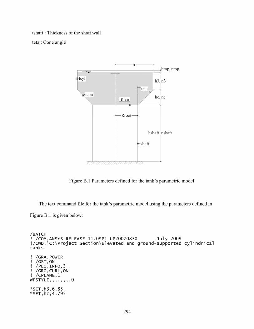
294

tshaft : Thickness of the shaft wall

teta : Cone angle

Figure B.1 Parameters defined for the tank’s parametric model

The text command file for the tank’s parametric model using the parameters defined in

Figure B.1 is given below:

/BATCH ! /COM,ANSYS RELEASE 11.0SP1 UP20070830 July 2009 !/CWD,'C:\Project Section\Elevated and ground-supported cylindrical tanks' ! /GRA,POWER ! /GST,ON ! /PLO,INFO,3 ! /GRO,CURL,ON ! /CPLANE,1 WPSTYLE,,,,,,,,0 *SET,h3,6.85 *SET,hc,4.795

295

*SET,rt,10.6175 *SET,rroot,5.8225 *SET,hshaft,15.8 *SET,tcyl,0.0088307 *SET,tcon,0.024511 *SET,htop,0.5 *SET,mfloor,12760 *SET,mring,7818 *SET,tfloor,0.3302 *SET,tshaft,0.381 !teta=(atan((rt-rroot)/hc))*180/3.1415 *SET,teta,(atan((rt-rroot)/hc))*180/3.1415 *SET,ntop,2 *SET,n3,14 *SET,nc,14 *SET,nshaft,13 *SET,nr,14 *SET,MINFLOOR , -h3-hc-0.385*hshaft-0.5*hshaft/nshaft *SET,MAXFLOOR , -h3-hc-0.385*hshaft+0.5*hshaft/nshaft *SET,massfloor,56*1270 *SET,massring,56*7818 !************************Element type ET,1,FLUID80 KEYOPT,1,2,1 ET,2,MASS21 KEYOPT,2,1,0 KEYOPT,2,2,0 KEYOPT,2,3,0 ET,3,SHELL63 KEYOPT,3,1,0 KEYOPT,3,2,0 KEYOPT,3,3,0 KEYOPT,3,5,0 KEYOPT,3,6,0 KEYOPT,3,7,0 KEYOPT,3,8,0 KEYOPT,3,9,0 KEYOPT,3,11,0 !****************Material Properties MPTEMP,,,,,,,, MPTEMP,1,0 MPDATA,DENS,1,,1000 MPTEMP,,,,,,,, MPTEMP,1,0 MPDATA,EX,1,,2.1e9 MPDATA,PRXY,1,, MPTEMP,,,,,,,, MPTEMP,1,0 MPDATA,DENS,2,,7898 MPTEMP,,,,,,,, MPTEMP,1,0 MPDATA,EX,2,,2e11 MPDATA,PRXY,2,,0.3 MPTEMP,,,,,,,,

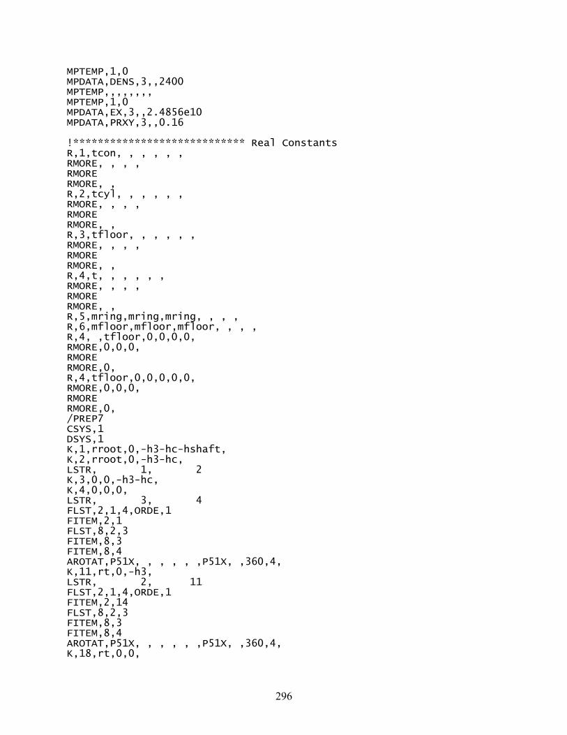
296

MPTEMP,1,0 MPDATA,DENS,3,,2400 MPTEMP,,,,,,,, MPTEMP,1,0 MPDATA,EX,3,,2.4856e10 MPDATA,PRXY,3,,0.16 !**************************** Real Constants R,1,tcon, , , , , , RMORE, , , , RMORE RMORE, , R,2,tcyl, , , , , , RMORE, , , , RMORE RMORE, , R,3,tfloor, , , , , , RMORE, , , , RMORE RMORE, , R,4,t, , , , , , RMORE, , , , RMORE RMORE, , R,5,mring,mring,mring, , , , R,6,mfloor,mfloor,mfloor, , , , R,4, ,tfloor,0,0,0,0, RMORE,0,0,0, RMORE RMORE,0, R,4,tfloor,0,0,0,0,0, RMORE,0,0,0, RMORE RMORE,0, /PREP7 CSYS,1 DSYS,1 K,1,rroot,0,-h3-hc-hshaft, K,2,rroot,0,-h3-hc, LSTR, 1, 2 K,3,0,0,-h3-hc, K,4,0,0,0, LSTR, 3, 4 FLST,2,1,4,ORDE,1 FITEM,2,1 FLST,8,2,3 FITEM,8,3 FITEM,8,4 AROTAT,P51X, , , , , ,P51X, ,360,4, K,11,rt,0,-h3, LSTR, 2, 11 FLST,2,1,4,ORDE,1 FITEM,2,14 FLST,8,2,3 FITEM,8,3 FITEM,8,4 AROTAT,P51X, , , , , ,P51X, ,360,4, K,18,rt,0,0,

297

LSTR, 11, 18 FLST,2,1,4,ORDE,1 FITEM,2,26 FLST,8,2,3 FITEM,8,4 FITEM,8,3 AROTAT,P51X, , , , , ,P51X, ,360,4, K,25,rt,0,htop, LSTR, 18, 25 FLST,2,1,4,ORDE,1 FITEM,2,38 FLST,8,2,3 FITEM,8,3 FITEM,8,4 AROTAT,P51X, , , , , ,P51X, ,360,4, LSTR, 3, 2 FLST,2,1,4,ORDE,1 FITEM,2,50 FLST,8,2,3 FITEM,8,3 FITEM,8,4 AROTAT,P51X, , , , , ,P51X, ,360,4, WPCSYS,-1 CONE,rroot,rt,-h3-hc,-h3,0,360, CONE,rt,rt,0,-h3,0,360, DSYS,0 KWPLAN,-1, 15, 29, 18 FLST,2,2,6,ORDE,2 FITEM,2,1 FITEM,2,-2 VSBW,P51X KWPLAN,-1, 13, 24, 31 FLST,2,4,6,ORDE,2 FITEM,2,3 FITEM,2,-6 VSBW,P51X WPCSYS,-1 FLST,5,8,6,ORDE,4 FITEM,5,1 FITEM,5,-2 FITEM,5,7 FITEM,5,-12 VSEL,S, , ,P51X ASLV,S LSLA,S KSLL,S NUMMRG,KP, , , ,LOW ALLSEL,ALL ASLV,U LSLA,S KSLL,S NUMMRG,KP, , , ,LOW ALLSEL,ALL ASLV,U FLST,5,4,5,ORDE,2 FITEM,5,1 FITEM,5,-4 CM,_Y,AREA

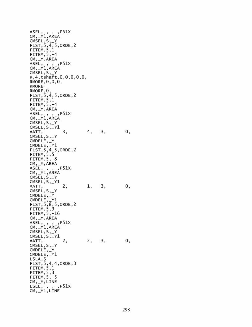
298

ASEL, , , ,P51X CM,_Y1,AREA CMSEL,S,_Y FLST,5,4,5,ORDE,2 FITEM,5,1 FITEM,5,-4 CM,_Y,AREA ASEL, , , ,P51X CM,_Y1,AREA CMSEL,S,_Y R,4,tshaft,0,0,0,0,0, RMORE,0,0,0, RMORE RMORE,0, FLST,5,4,5,ORDE,2 FITEM,5,1 FITEM,5,-4 CM,_Y,AREA ASEL, , , ,P51X CM,_Y1,AREA CMSEL,S,_Y CMSEL,S,_Y1 AATT, 3, 4, 3, 0, CMSEL,S,_Y CMDELE,_Y CMDELE,_Y1 FLST,5,4,5,ORDE,2 FITEM,5,5 FITEM,5,-8 CM,_Y,AREA ASEL, , , ,P51X CM,_Y1,AREA CMSEL,S,_Y CMSEL,S,_Y1 AATT, 2, 1, 3, 0, CMSEL,S,_Y CMDELE,_Y CMDELE,_Y1 FLST,5,8,5,ORDE,2 FITEM,5,9 FITEM,5,-16 CM,_Y,AREA ASEL, , , ,P51X CM,_Y1,AREA CMSEL,S,_Y CMSEL,S,_Y1 AATT, 2, 2, 3, 0, CMSEL,S,_Y CMDELE,_Y CMDELE,_Y1 LSLA,S FLST,5,4,4,ORDE,3 FITEM,5,1 FITEM,5,3 FITEM,5,-5 CM,_Y,LINE LSEL, , , ,P51X CM,_Y1,LINE

299

CMSEL,,_Y !************************Mesh divisions LESIZE,_Y1, , ,nshaft, , , , ,0 FLST,5,4,4,ORDE,2 FITEM,5,14 FITEM,5,-17 CM,_Y,LINE LSEL, , , ,P51X CM,_Y1,LINE CMSEL,,_Y LESIZE,_Y1, , ,nc, , , , ,0 FLST,5,4,4,ORDE,2 FITEM,5,26 FITEM,5,-29 CM,_Y,LINE LSEL, , , ,P51X CM,_Y1,LINE CMSEL,,_Y LESIZE,_Y1, , ,n3, , , , ,0 FLST,5,4,4,ORDE,2 FITEM,5,38 FITEM,5,-41 CM,_Y,LINE LSEL, , , ,P51X CM,_Y1,LINE CMSEL,,_Y LESIZE,_Y1, , ,ntop, , , , ,0 FLST,5,20,4,ORDE,14 CM,_Y,LINE LSEL, , , ,P51X CM,_Y1,LINE CMSEL,,_Y LESIZE,_Y1, , ,nr, , , , ,0 ASLV,U FLST,5,4,5,ORDE,2 FITEM,5,17 FITEM,5,-20 CM,_Y,AREA ASEL, , , ,P51X CM,_Y1,AREA CMSEL,S,_Y CMSEL,S,_Y1 AATT, 3, 3, 3, 0, CMSEL,S,_Y CMDELE,_Y CMDELE,_Y1 MSHAPE,0,2D MSHKEY,1 FLST,5,20,5,ORDE,2 FITEM,5,1 FITEM,5,-20 CM,_Y,AREA ASEL, , , ,P51X CM,_Y1,AREA CHKMSH,'AREA' CMSEL,S,_Y AMESH,_Y1

300

CMDELE,_Y CMDELE,_Y1 CMDELE,_Y2 /UI,MESH,OFF NUMMRG,NODE, , , ,LOW ALLSEL,ALL CSYS,1 ALLSEL,ALL CSYS,1 NSEL,S,LOC,Z,-h3-hc NSEL,R,LOC,X,rroot /GO KNODE,0,all ASLV,U LSLA,S KSLL,S KSLN,A ALLSEL,ALL KSLN,S ALLSEL,ALL ASLV,U LSLA,S KSLL,S FLST,5,16,3,ORDE,16 KSEL,U, , ,P51X KSLN,A ALLSEL,ALL ASLV,S LSLA,S KSLL,U KSLN,U ALLSEL,ALL ASLV,S LSLA,S KSLL,U NUMMRG,KP, , , ,LOW ALLSEL,ALL NSEL,S,LOC,Z,minfloor,maxfloor KNODE,0,all ALLSEL,ALL ASLV,U NSEL,ALL ALLSEL,ALL ASLV,S LSLA,S KSLL,U KSEL,R,LOC,Z,-h3-hc KSEL,R,LOC,X,rroot FLST,5,80,3,ORDE,22 CM,_Y,KP KSEL, , , ,P51X CM,_Y1,KP CMSEL,S,_Y CMSEL,S,_Y1 KATT, 1, 5, 2, 0 CMSEL,S,_Y CMDELE,_Y CMDELE,_Y1

301

FLST,2,80,3,ORDE,22 KMESH,all ALLSEL,ALL ESEL,S,TYPE,,2 ALLSEL,ALL KSEL,S,LOC,Z,minfloor,maxfloor FLST,5,80,3,ORDE,6 CM,_Y,KP KSEL, , , ,P51X CM,_Y1,KP CMSEL,S,_Y CMSEL,S,_Y1 KATT, 1, 6, 2, 0 CMSEL,S,_Y CMDELE,_Y CMDELE,_Y1 FLST,2,80,3,ORDE,6 KMESH,all ALLSEL,ALL NUMMRG,NODE, , , ,LOW /UI,MESH,OFF ASLV,S LSLA,S FLST,5,12,4,ORDE,4 CM,_Y,LINE LSEL, , , ,P51X CM,_Y1,LINE CMSEL,,_Y LESIZE,_Y1, , ,nr, , , , ,0 FLST,5,4,4,ORDE,4 CM,_Y,LINE LSEL, , , ,P51X CM,_Y1,LINE CMSEL,,_Y LESIZE,_Y1, , ,n3, , , , ,0 FLST,5,3,4,ORDE,3 CM,_Y,LINE LSEL, , , ,P51X CM,_Y1,LINE CMSEL,,_Y LESIZE,_Y1, , ,n3, , , , ,0 FLST,5,5,4,ORDE,5 CM,_Y,LINE LSEL, , , ,P51X CM,_Y1,LINE CMSEL,,_Y LESIZE,_Y1, , ,nc, , , , ,0 MSHAPE,0,3D FLST,5,8,6,ORDE,4 CM,_Y,VOLU VSEL, , , ,P51X CM,_Y1,VOLU CHKMSH,'VOLU' CMSEL,S,_Y VMESH,_Y1 CMDELE,_Y CMDELE,_Y1 CMDELE,_Y2

302

/UI,MESH,OFF ACEL,0,0,9.807, LSEL,S,LOC,Z,-hc-h3-hshaft NSLL,S,1 FLST,2,80,1,ORDE,8 /GO D,all, , , , , ,UX,UY,UZ, , , ALLSEL,ALL CSYS,1 FLST,2,45673,1,ORDE,4 NROTAT,all NSEL,S,LOC,Z,0,-h3 CPINTF,UX,0.0001, NSEL,R,LOC,Z,-h3 CPINTF,UZ,0.0001, ALLSEL,ALL NSEL,S,LOC,Z,-h3-hc,-h3-0.05 NSEL,S,LOC,X,rroot,rt ALLSEL,ALL NSEL,S,LOC,Z,-h3-hc,-h3-0.05 NSEL,R,LOC,X,rroot,rt CSYS,1 FLST,2,5660,1,ORDE,971 NROTAT,all nmodif,all, , , , , ,teta CPINTF,UX,0.0001, ALLSEL,ALL NSEL,S,LOC,Z,-h3-hc CPINTF,UZ,0.0001, ALLSEL,ALL ESEL,S,TYPE,,1 NSLE,S NUMMRG,NODE, , , ,LOW ALLSEL,ALL LSEL,S,LOC,Z,-hc-h3-hshaft NSLL,S,1 /GO D,all, , , , , ,UX,UY,UZ, , , ALLSEL,ALL WPSTYLE,,,,,,,,0 NSEL,S,LOC,Z,-h3-hc NSEL,R,LOC,X,rroot CSYS,1 FLST,2,112,1,ORDE,21 NROTAT,all ALLSEL,ALL

303

B.2 Text command file of the post-processor “POST-CYL”

The text command file of the post-processor “POST-CYL” is given below:

!/POST-PROCESSOR "POST-CYL"

*DIM,EPRESSURE,ARRAY,n3,1

*Do,k,1,n3,1

ESLV,S

NSEL,S,LOC,Z,0-(k-1)*h3/n3

NSEL,R,LOC,X,rt

ESLN,R

NSEL,S,LOC,Z,0-(k-1-1)*h3/n3

ESLN,U

/POST1

PLESOL, SMISC,1, 0,1.0

*GET,EPRESSURE(k),PLNSOL,0,MAX

ALLSEL,ALL

*ENDDO

Finish

*CFOPEN,PSCyl

*VWRITE,EPRESSURE(1)

(F15.4)

B.3 Text command file of the post-processor “POST-CON”

The text command file of the post-processor “POST-CON” is given below:

!/POST-PROCESSOR "POST-CON"

*DIM,EPRESSURE,ARRAY,nc,1

*Do,k,1,nc,1

ESLV,S

NSEL,S,LOC,Z,-h3-k*hc/nc

NSEL,R,LOC,X,((rt-rroot)*(hc-k*hc/nc)/hc)+rroot

ESLN,R

NSEL,S,LOC,Z,-h3-(k+1)*hc/nc

ESLN,U

ESEL,U,TYPE,,3

304

/POST1



ALLSEL,ALL

*ENDDO

Finish

*CFOPEN,PScone


(F15.4)

B.4 Text command file of the post-processor “POST-FLOOR”

The text command file of the post-processor “POST-FLOOR” is given below:

!/POST-PROCESSOR "POST-FLOOR"

*DIM,EPRESSURE,ARRAY,nr,1

*Do,k,1,nr,1

ESLV,S

NSEL,S,LOC,Z,-h3-hc

NSEL,R,LOC,X,rroot-(k-1)*rroot/nr

ESLN,R

NSEL,R,LOC,X,rroot-(k-2)*rroot/nr

ESLN,U

ESEL,U,TYPE,,3

/POST1



ALLSEL,ALL

*ENDDO

Finish

*CFOPEN,PSfloor


(F15.4)

305

APPENDIX C

RESULTS OF THE PARAMETRIC STUDY ON LIQUID-FILLED

CONICAL ELEVATED TANKS

C.1 Hydrodynamic pressure distribution graphs

The normalized convective and impulsive pressure graphs obtained through the parametric

study corresponding to the three different ranges of shaft stiffness considered are given in

Figures C.1 through C.26.

306

-1.0

-0.8

-0.6

-0.4

-0.2

0.0 0.1 0.2 0.3 0.4 0.5


Wat

er d

epth

rat

io (

h/h

l)

h/hl=-0.68


1.30

1.19

1.08

0.96

0.85 0.740.63

0.51

Rroot/h3=0.4

(a)

-1.0

-0.8

-0.6

-0.4

-0.2

0.0

0.0 0.1 0.2 0.3 0.4 0.5 0.6 0.7


Wat

er d

epth

rat

io (

h/h

l)


h/hl=-0.68

1.30

1.19

1.08

0.96

0.85 0.74 0.63 0.51 Rroot/h3=0.40

(b)



307

-1.0

-0.8

-0.6

-0.4

-0.2

0.0 0.1 0.2 0.3 0.4 0.5


Wat

er d

epth

rat

io (

h/h

l)

h/hl=-0.645


1.30

1.19

1.08 0.960.85

0.74

0.63 0.51

Rroot/h3=0.40

(a)

-1.0

-0.8

-0.6

-0.4

-0.2

0.0

0.0 0.1 0.2 0.3 0.4 0.5 0.6Normalized wall pressure (Pi/Sai/WL)*103, s2/m3

Wat

er d

epth

rat

io (

h/h

l)

h/hl=-0.645


1.30

1.19

0.96

0.85 0.74 0.63 0.51 Rroot/h3=0.401.08

(b)



308

-1.0

-0.8

-0.6

-0.4

-0.2

0.0 0.1 0.2 0.3 0.4 0.5


Wat

er d

epth

rat

io (

h/h

l)

h/hl=-0.615


1.30

1.19

1.080.96

0.85 0.740.63 0.51

Rroot/h3=0.40

(a)

-1.0

-0.8

-0.6

-0.4

-0.2

0.0

0.0 0.1 0.2 0.3 0.4 0.5


Wat

er d

epth

rat

io (

h/h

l)

h/hl=-0.615


1.30

1.190.96

0.85

0.74 0.63 0.51 Rroot/h3=0.401.08

(b)



309

-1.0

-0.8

-0.6

-0.4

-0.2

0.0 0.1 0.2 0.3 0.4


Wat

er d

epth

rat

io (

h/h

l)

h/hl=-0.59


1.30

1.191.08

0.960.85

0.74

0.63 0.51

Rroot/h3=0.4

(a)

-1.0

-0.8

-0.6

-0.4

-0.2

0.0

0.0 0.1 0.2 0.3 0.4 0.5


Wat

er d

epth

rat

io (

h/h

l)


1.30

1.19

0.96

0.85

0.74 0.63 0.51 Rroot/h3=0.40

1.08

(b)



310

-1.0

-0.8

-0.6

-0.4

-0.2

0.0 0.1 0.2 0.3 0.4


Wat

er d

epth

rat

io (

h/h

l)

h/hl=-0.56


1.30

1.19

1.08

0.960.85 0.74

0.63 0.51

Rroot/h3=0.4

(a)

-1.0

-0.8

-0.6

-0.4

-0.2

0.0

0.0 0.1 0.2 0.3 0.4


Wat

er d

epth

rat

io (

h/h

l)

h/hl=-0.56


1.30

1.19

0.96

0.85

0.74

0.63 0.51 Rroot/h3=0.40

1.08

(b)



311

-1.0

-0.8

-0.6

-0.4

-0.2

0.0 0.1 0.2 0.3 0.4


Wat

er d

epth

rat

io (

h/h

l)

h/hl=-0.54


1.30

1.19

1.08

0.960.85

0.74

0.630.51

Rroot/h3=0.4

(a)

-1.0

-0.8

-0.6

-0.4

-0.2

0.0

0.0 0.1 0.2 0.3 0.4


Wat

er d

epth

rat

io (

h/h

l)

h/hl=-0.54


1.30

1.19

0.96

0.85

0.74

0.63 0.51 Rroot/h3=0.40

1.08

(b)



312

-1.0

-0.8

-0.6

-0.4

-0.2

0.0 0.1 0.2 0.3 0.4


Wat

er d

epth

rat

io (

h/h

l)

h/hl=-0.52


1.30

1.19

1.08 0.96

0.850.74

0.630.51

Rroot/h3=0.4

(a)

-1.0

-0.8

-0.6

-0.4

-0.2

0.0

0.0 0.1 0.2 0.3


Wat

er d

epth

rat

io (

h/h

l)

h/hl=-0.52


1.30

1.19

0.96

0.85

0.74 0.63 0.51 Rroot/h3=0.40

1.08

(b)



313

-1.0

-0.8

-0.6

-0.4

-0.2

0.0 0.1 0.2 0.3


Wat

er d

epth

rat

io (

h/h

l)

h/hl=-0.50


1.30

1.19

1.080.96 0.85

0.74

0.63 0.51

Rroot/h3=0.40

(a)

-1.0

-0.8

-0.6

-0.4

-0.2

0.0

0.0 0.1 0.2 0.3


Wat

er d

epth

rat

io (

h/h

l)

h/hl=-0.50


1.30

1.190.96

0.85

0.74

0.63 0.51 Rroot/h3=0.40

1.08

(b)



314

-1.0

-0.8

-0.6

-0.4

-0.2

0.0 0.1 0.2 0.3 0.4 0.5 0.6


Wat

er d

epth

rat

io (

h/h

l)

h/hl=-0.714


1.30

1.19

1.08 0.960.85

0.740.63 0.51

Rroot/h3=0.4

(a)

-1.0

-0.8

-0.6

-0.4

-0.2

0.0

0.0 0.1 0.2 0.3 0.4 0.5 0.6


Wat

er d

epth

rat

io (

h/h

l)

h/hl=-0.714


1.30

1.19

1.08

0.96

0.85

0.74 0.63 0.51 Rroot/h3=0.4

(b)



315

-1.0

-0.8

-0.6

-0.4

-0.2

0.0 0.1 0.2 0.3 0.4 0.5 0.6


Wat

er d

epth

rat

io (

h/h

l)

h/hl=-0.68


1.30

1.19

1.08

0.960.85

0.740.63 0.51

Rroot/h3=0.4

(a)

-1.0

-0.8

-0.6

-0.4

-0.2

0.0

0.0 0.1 0.2 0.3 0.4 0.5 0.6


Wat

er d

epth

rat

io (

h/h

l)


h/hl=-0.68

1.30

1.19

1.08

0.96

0.85

0.74 0.63 0.51 Rroot/h3=0.4

(b)



316

-1.0

-0.8

-0.6

-0.4

-0.2

0.0 0.1 0.2 0.3 0.4 0.5Normalized wall pressure (Pc/Sac/WL)*103, s2/m3

Wat

er d

epth

rat

io (

h/h

l)

h/hl=-0.645


1.30

1.19

1.08

0.96

0.85 0.740.63 0.51

Rroot/h3=0.4

(a)

-1.0

-0.8

-0.6

-0.4

-0.2

0.0

0.0 0.1 0.2 0.3 0.4 0.5


Wat

er d

epth

rat

io (

h/h

l)

h/hl=-0.645


1.30

1.19

1.08 0.96

0.85

0.74 0.63 0.51 Rroot/h3=0.4

(b)



317

-1.0

-0.8

-0.6

-0.4

-0.2

0.0 0.1 0.2 0.3 0.4 0.5


Wat

er d

epth

rat

io (

h/h

l)

h/hl=-0.615


1.30

1.19

1.08

0.960.85

0.740.63 0.51

Rroot/h3=0.4

(a)

-1.0

-0.8

-0.6

-0.4

-0.2

0.0

0.0 0.1 0.2 0.3 0.4


Wat

er d

epth

rat

io (

h/h

l)

h/hl=-0.615


1.30

1.19

1.080.96

0.85

0.74 0.63 0.51 Rroot/h3=0.4

(b)



318

-1.0

-0.8

-0.6

-0.4

-0.2


Wat

er d

epth

rat

io (

h/h

l)

h/hl=-0.59


1.30

1.19

1.08

0.96

0.85 0.740.63 0.51

Rroot/h3=0.4

(a)

-1.0

-0.8

-0.6

-0.4

-0.2

0.0

0.0 0.1 0.2 0.3 0.4


Wat

er d

epth

rat

io (

h/h

l)

h/hl=-0.59


1.30

1.19

1.08 0.96

0.85

0.74

0.63 0.51 Rroot/h3=0.40

(b)



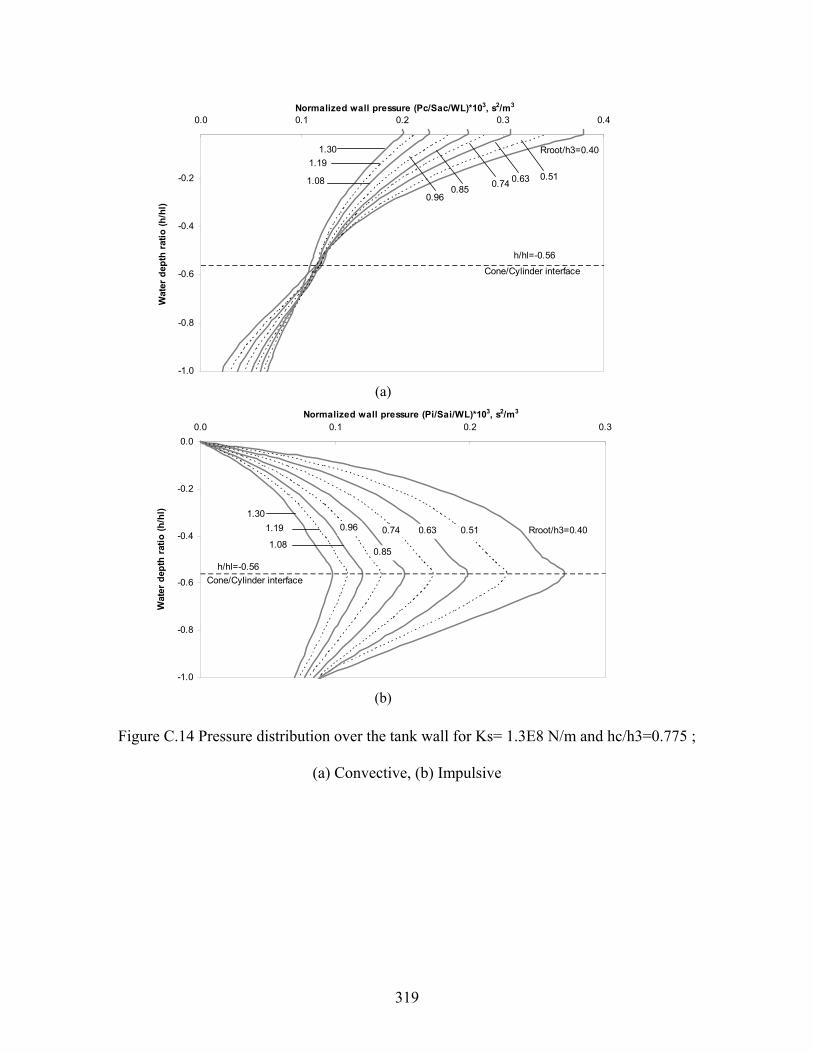
319

-1.0

-0.8

-0.6

-0.4

-0.2

0.0 0.1 0.2 0.3 0.4Normalized wall pressure (Pc/Sac/WL)*103, s2/m3

Wat

er d

epth

rat

io (

h/h

l)

h/hl=-0.56


1.30

1.19

1.08

0.960.85

0.74 0.63 0.51

Rroot/h3=0.40

(a)

-1.0

-0.8

-0.6

-0.4

-0.2

0.0

0.0 0.1 0.2 0.3Normalized wall pressure (Pi/Sai/WL)*103, s2/m3

Wat

er d

epth

rat

io (

h/h

l)

h/hl=-0.56


1.30

1.19

1.08

0.96

0.85

0.74 0.63 0.51 Rroot/h3=0.40

(b)



320

-1.0

-0.8

-0.6

-0.4

-0.2

0.0 0.1 0.2 0.3 0.4


Wat

er d

epth

rat

io (

h/h

l)

h/hl=-0.54


1.30

1.19

1.08

0.960.85 0.74

0.63 0.51

Rroot/h3=0.4

(a)

-1.0

-0.8

-0.6

-0.4

-0.2

0.0

0.0 0.1 0.2 0.3


Wat

er d

epth

rat

io (

h/h

l)

h/hl=-0.54


1.30

1.19

1.08

0.96

0.85

0.74

0.63 0.51 Rroot/h3=0.4

(b)



321

-1.0

-0.8

-0.6

-0.4

-0.2


Wat

er d

epth

rat

io (

h/h

l)

h/hl=-0.52


1.30

1.19

1.08

0.960.85

0.740.63 0.51

Rroot/h3=0.4

(a)

-1.0

-0.8

-0.6

-0.4

-0.2

0.0


Wat

er d

epth

rat

io (

h/h

l)

h/hl=-0.52


1.30

1.19

1.08

0.96

0.85

0.74

0.63 0.51 Rroot/h3=0.40

(b)



322

-1.0

-0.8

-0.6

-0.4

-0.2

0.0 0.1 0.2 0.3 0.4


Wat

er d

epth

rat

io (

h/h

l)

h/hl=-0.50


1.30

1.19

1.080.96

0.85 0.740.63 0.51

Rroot/h3=0.40

(a)

-1.0

-0.8

-0.6

-0.4

-0.2

0.0

0.0 0.1 0.2Normalized wall pressure (Pi/Sai/WL)*103, s2/m3

Wat

er d

epth

rat

io (

h/h

l)

h/hl=-0.50


1.30

1.19

1.08

0.96

0.85

0.74

0.63 0.51 Rroot/h3=0.40

(b)



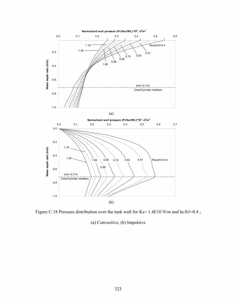
323

-1.0

-0.8

-0.6

-0.4

-0.2

0.0 0.1 0.2 0.3 0.4 0.5 0.6


Wat

er d

epth

rat

io (

h/h

l)

h/hl=-0.714


1.30

1.19

1.080.96

0.850.74 0.63

0.51

Rroot/h3=0.4

(a)

-1.0

-0.8

-0.6

-0.4

-0.2

0.0

0.0 0.1 0.2 0.3 0.4 0.5 0.6 0.7


Wat

er d

epth

rat

io (

h/h

l)

h/hl=-0.714


1.30

1.19

1.08

0.96

0.85 0.74 0.63 0.51 Rroot/h3=0.4

(b)



324

-1.0

-0.8

-0.6

-0.4

-0.2


Wat

er d

epth

rat

io (

h/h

l)

h/hl=-0.68


1.30

1.19

1.080.96 0.85

0.74 0.63 0.51

Rroot/h3=0.4

(a)

-1.0

-0.8

-0.6

-0.4

-0.2

0.0

0.0 0.1 0.2 0.3 0.4 0.5 0.6


Wat

er d

epth

rat

io (

h/h

l)


h/hl=-0.68

1.30

1.19

1.08

0.96

0.85 0.74 0.63 0.51 Rroot/h3=0.4

(b)



325

-1.0

-0.8

-0.6

-0.4

-0.2

0.0 0.1 0.2 0.3 0.4 0.5


Wat

er d

epth

rat

io (

h/h

l)

h/hl=-0.645


1.30

1.19

1.080.96

0.850.74 0.63 0.51

Rroot/h3=0.4

(a)

-1.0

-0.8

-0.6

-0.4

-0.2

0.0

0.0 0.1 0.2 0.3 0.4 0.5 0.6


Wat

er d

epth

rat

io (

h/h

l)

h/hl=-0.645


1.30

1.19

1.08

0.96

0.85

0.74 0.63 0.51 Rroot/h3=0.4

(b)



326

-1.0

-0.8

-0.6

-0.4

-0.2

0.0 0.1 0.2 0.3 0.4 0.5


Wat

er d

epth

rat

io (

h/h

l)


1.30

1.19

1.080.96 0.85

0.74 0.63 0.51

Rroot/h3=0.4

(a)

-1.0

-0.8

-0.6

-0.4

-0.2

0.0

0.0 0.1 0.2 0.3 0.4 0.5


Wat

er d

epth

rat

io (

h/h

l)

h/hl=-0.615


1.30

1.19

1.080.96

0.85

0.74 0.63 0.51 Rroot/h3=0.4

(b)



327

-1.0

-0.8

-0.6

-0.4

-0.2


Wat

er d

epth

rat

io (

h/h

l)

h/hl=-0.59


1.30

1.19

1.08

0.960.85 0.74

0.63 0.51

Rroot/h3=0.4

(a)

-1.0

-0.8

-0.6

-0.4

-0.2

0.0

0.0 0.1 0.2 0.3 0.4Normalized wall pressure (Pi/Sai/WL)*103, s2/m3

Wat

er d

epth

rat

io (

h/h

l)

h/hl=-0.59


1.30

1.19

1.080.96

0.85

0.74 0.63 0.51 Rroot/h3=0.4

(b)



328

-1.0

-0.8

-0.6

-0.4

-0.2


Wat

er d

epth

rat

io (

h/h

l)

h/hl=-0.56


1.30

1.19

1.08 0.96 0.850.74

0.63 0.51

Rroot/h3=0.4

(a)

-1.0

-0.8

-0.6

-0.4

-0.2

0.0

0.0 0.1 0.2 0.3 0.4


Wat

er d

epth

rat

io (

h/h

l)

h/hl=-0.56


1.30

1.19

1.08

0.96

0.85

0.74

0.63 0.51 Rroot/h3=0.40

(b)



329

-1.0

-0.8

-0.6

-0.4

-0.2

0.0 0.1 0.2 0.3 0.4


Wat

er d

epth

rat

io (

h/h

l)

h/hl=-0.54


1.30

1.19

1.08

0.960.85

0.740.63 0.51

Rroot/h3=0.4

(a)

-1.0

-0.8

-0.6

-0.4

-0.2

0.0

0.0 0.1 0.2 0.3 0.4Normalized wall pressure (Pi/Sai/WL)*103, s2/m3

Wat

er d

epth

rat

io (

h/h

l)

h/hl=-0.54


1.30

1.19

1.080.85

0.74

0.63 0.51 Rroot/h3=0.40

0.96

(b)



330

-1.0

-0.8

-0.6

-0.4

-0.2

0.0 0.1 0.2 0.3 0.4


Wat

er d

epth

rat

io (

h/h

l)

h/hl=-0.52


1.30

1.19

1.08

0.960.85

0.740.63 0.51

Rroot/h3=0.40

(a)

-1.0

-0.8

-0.6

-0.4

-0.2

0.0


Wat

er d

epth

rat

io (

h/h

l)

h/hl=-0.52


1.301.19

1.080.85

0.74

0.63 0.51 Rroot/h3=0.40

0.96

(b)



331

-1.0

-0.8

-0.6

-0.4

-0.2

0.0 0.1 0.2 0.3


Wat

er d

epth

rat

io (

h/h

l)

h/hl=-0.50


1.30

1.19

1.080.96 0.85

0.740.63 0.51

Rroot/h3=0.40

(a)

-1.0

-0.8

-0.6

-0.4

-0.2

0.0

0.0 0.1 0.2 0.3


Wat

er d

epth

rat

io (

h/h

l)

h/hl=-0.50


1.30

1.19

1.08

0.85

0.74

0.63 0.51 Rroot/h3=0.40

0.96

(b)



332

REFERENCES

Abromowitz, M., and Stegun, T.A., 1972, “Handbook of mathematical functions with formulas,

graphs and mathematical tables”, 10. Applied mathematics series, 55. Washington: National

Bureau of Standards.

ACI Committee 350-01, 2001, “Code requirements for environmental engineering concrete

structures (ACI 350-01) and commentary (ACI 350R-01)”, American Concrete Institute,

Farmington Hills, MI, U.S.A.

ACI Committee 350.3-06, 2006, “Seismic design of liquid-containing concrete structures (ACI

350.3-06) and commentary (ACI 350.3R-06)”, American Concrete Institute, Farmington Hills,

MI, U.S.A.

ACI Committee 371, 2008, ”Guide for the analysis, design and construction of elevated concrete

and composite steel-concrete water storage tanks (ACI 371R-08)”, American Concrete Institute,

Farmington Hills, MI, U.S.A.

Anshel, J.S., 1999, “Kobe earthquake of January 17, 1995. Lifeline performance. 1995”, ASCE

Publication.

Aoyagi, M., and Shiomi, 1985, “Studies on menshin structures”, Report of Central Research

Institute of Electric Power Industry, 385010.

American Petroleum Institute, API 620, 1998, “Design and construction of large, welded, low-

pressure storage tanks”, American Petroleum Institute Standard, Washington D.C., U.S.A.

American Petroleum Institute, API 650, 1998, “Welded steel tanks for oil storage”, American

Petroleum Institute Standard, Washington D.C., U.S.A.

333

Arias, A., 1970, “A measure of earthquake intensity”, Seismic Design for Nuclear Power Plants,

MIT Press, Cambridge.

American Society of Civil Engineers (ASCE), 1980, “Structural analysis and design of nuclear

plant facilities”, ASCE Manuals and Reports on Engineering Practice No. 58, New York, New

York.

American Society of Civil Engineers (ASCE), 1998, “Seismic analysis of safety-related nuclear

structures and commentary”, ASCE 4-98, Reston, VA.

American Society of Civil Engineers (ASCE), Structural Engineering Institute, 2006, “Minimum

design loads for buildings and other structures”, ASCE/SEI 7-05, Reston, VA.

American Society of Civil Engineers (ASCE), Structural Engineering Institute, 2010, “Minimum

design loads for buildings and other structures”, ASCE/SEI 7-10, Reston, VA.

American Water Works Association (AWWA), 1984 and 2005, “Welded steel tanks for water

storage”, AWWA D100, CO.

American Water Works Association (AWWA), 1995, “Wire and strand-wounded circular

prestressed concrete water tanks”, AWWA D110, Denver, CO.

American Water Works Association (AWWA), 1995, “Circular prestressed concrete water tanks

with circumferential tendons”, AWWA D115, Denver, CO.

Balendra, T., Ang, K.K., Paramasivan, P., and Lee, S.L., 1982, ”Seismic design of flexible

cylindrical liquid storage tanks”, Earthquake Engineering and Structural Dynamics, 10, 477-496.

Barton, D.C., and Parker, J.V., 1987, ”Finite element analysis of the seismic response of

anchored and unanchored liquid storage tanks”, Earthquake Engineering and Structural

Dynamics, 15, 299-322.

334

Blakeley, R.W.G., Cormack, L.G., and Stockwell, M.J., 1980, “Mechanical energy dissipation

devices”, Bull. N. Z. Natl. Soc. Earthquake Eng., 13, 264 – 268.

Bleiman, D., and Kim, S., 1993, “Base isolation of high volume elevated water tanks”, Proc.,

Seminar on Seismic Isolation, Passive Energy Dissipation and Active Control, ATC 17-1,

Applied Technology Council, Redwood City, Calif.

Bo, L., and Jia-xiang, T., 1994, “Vibration studies of base-isolated liquid storage tanks”, Comp.

and Struct., 52(5), 1051-1059.

BS 8007, 1987, “Code of practice for design of concrete structures for retaining aqueous

liquids”, British Standard Institution.

Chalhoub, M.S., and Kelly, J.M., 1990, “Shake table test of cylindrical water tanks in base-

isolated structures”, J. Engrg. Mech., ASCE, 116(7), 1451-1472.

Chandrasekaran, A.R., and Krishna, 1965, “Water towers in seismic zones”, 1965 Proceedings of

the Third World Conference on Earthquake Engineering, New Zealand, IV, 161-171.

Chen, J.Z., and Kianoush, M.R., 2005, “Seismic response of concrete rectangular tanks for liquid

containing structures”, Canadian Journal of Civil Engineering, 32, 739-752.

Chopra, A.K., 2000, ”Dynamics of structures: theory and applications to earthquake

engineering”, 2nd edition, Prentice-Hall.

Clough, R.W., and Clough, D.P., 1977, “Seismic response of flexible cylindrical tanks”, Paper K

5/1 Trans. 4th International Conference on Structural Mechanics in Reactor Technology, San

Francisco, CA.

Clough, R.W., Niwa, A., and Clough, D.P., 1979, “Experimental seismic study of cylindrical

tanks”, Journal of the Structural Division, ASCE, Vol. 105, No. 12, pp. 2565-2590.

335

Dogangun, A., Durmus, A., and Ayvaz, Y., 1997, “Earthquake analysis of flexible rectangular

tanks using the Lagrangian fluid finite element“, Euro. J. Mech.-A/Solids, 16: 165-182.

Dogangun, A., and Livaoglu, R., 2004, “Hydrodynamic pressures acting on the walls of

rectangular fluid containers“, Structural Engineering and Mechanics, 17 (2), 203-214.

Dutta, S.C., Dutta, S., and Roy, R., 2009, “Dynamic behavior of R/C elevated tanks with soil-

structure interaction“, Journal of Engineering Structures, 31, 2617-2629.

European Committee for Standardization (ECS), 1998 and 2006, “Design provisions for

earthquake resistance of structures, Part 1– General rules and Part 4 – Silos, tanks and pipelines”,

Eurocode 8, Brussels, Belgium.

Edwards, N., 1969, “A procedure for the dynamic analysis of thin walled cylindrical liquid

storage tanks”, Ph.D. Thesis, University of Michigan, Ann Arbor, MI.

El Damatty, A.A., Mirza, F.A., and Korol, R.M., 1997A, ”Stability of imperfect steel conical

tanks under hydrostatic loading”, J. Struct. Engng., ASCE, 123, 703-712.

El Damatty, A.A., Korol, R.M., and Mirza, F.A., 1997B, ”Stability of elevated liquid-filled

conical tanks under seismic loading, Part I—Theory”, Earthquake Eng. Struct. Dyn., 26, 1191–

1208.

El Damatty, A.A., Korol, R.M., and Mirza, F.A., 1997C, ”Stability of elevated liquid-filled

conical tanks under seismic loading, Part II —Applications”, Earthquake Eng. Struct. Dyn., 26,

1209–1229.

El Damatty, A.A., Korol, R.M., and Tang, L.M., 2000, “The sloshing response of conical tanks”,

Proceedings of World Conference on Earthquake Engineering, Paper No. 966, Topic No. 7, New

Zealand.

336

El Damatty, A.A., Saafan, M.S., and Sweedan, A.M.I., 2005, ”Experimental study conducted on

a liquid-filled combined conical tank model”, Journal of Thin Walled Structures, 43, 1398–417.

Epstein, H.I., 1976, “Seismic design of liquid storage tanks”, Journal of the Structural Division,

102 (9): 1659-1673.

Fischer, F.D., 1979, “Dynamic fluid effects in liquid-filled flexible cylindrical tanks“,

Earthquake Engng. Struct. Dyn., 7, 587-601.

Flugge, W., 1960, “Stress in shells”, Springer-Verlag, Berlin.

Fox, D.W., and Kuttler, J.R., 1983, “Sloshing frequencies”, Journal of Applied Mathematics and

Physics, 34, 668-696.

Garcia, S.M., 1969, “Earthquake response analysis and seismic design of cylindrical tanks”,

Proceedings of the Fourth World Conference on Earthquake Engineering, Santiago, B-4, 169-

182.

Ghaemmaghami, A.R., Moslemi, M., and Kianoush, M.R., 2010, ”Dynamic behaviour of

concrete liquid tanks under horizontal and vertical ground motions using finite element method”,

9th US National and 10th Canadian Conf. on Earthquake Eng., Toronto, Canada.

Gupta, R.K., 1995, “Free vibrations of partially filled cylindrical tanks”, Journal of Engineering

Structures, 17(3), 221-230.

Haroun, M.A., 1980, ”Dynamic analyses of liquid storage tanks”, EERL¸ Report No. 80-04,

Earthquake Engineering Research Laboratory Report, California Institute of Technology,

Pasadenas, CA.

Haroun, M.A., 1983, “Vibration studies and tests of liquid storage tanks”, Earthquake Engng.

Struct. Dyn., 11, 190-206.

337

Haroun, M.A., 1984, “Stress analysis of rectangular walls under seismically induced

hydrodynamic loads”, Bulletin of the Seismological Society of America, 74(3), 1031-1041.

Haroun, M.A., and Ellaithy, H.M., 1985, ”Seismically induced fluid forces on elevated tanks”, J.

Tech. Topics Civil Eng., 1, 1-15.

Haroun, M.A., and Housner, G.W., 1981A, ”Seismic design of liquid storage tanks”, Journal of

the Technical Councils of ASCE, 107, 191- 207.

Haroun, M.A., and Housner, G.W., 1981B, ”Earthquake response of deformable liquid storage

tanks”, Journal of Applied Mechanics, ASME, 48, 411-418.

Haroun, M.A., and Tayel, M.A., 1985, ”Response of tanks to vertical seismic excitations”,

Earthquake Engng. Struct. Dyn., 13, 583-595.

Hazardous Material Technology Standards Committee: Fire Defense Agency, 1979, “Report on

causes of damage to petroleum tanks in Sendai Refinery of Tohoku Petroleum Company during

the 1978 earthquake of Miyagi prefecture”.

Housner, G.W., 1952, ”Spectrum intensities of strong motion earthquakes”, Proc. of Symposium

on Earthquake and Blunt Effects on Structures, Earthquake Engineering Research Institute.

Housner, G.W., 1957, ”Dynamic pressures on accelerated fluid containers”, Bulletin of the

Seismological Society of America 47(1), 15-37.

Housner, G.W., 1963, ”The dynamic behavior of water tanks”, Bulletin of the Seismological

Society of America 53(2), 381-389.

Housner, G.W., 1975, ”Measures of severity of earthquake ground shaking”, Proceedings of the

U.S. National Conference on Earthquake Engineering, EERI, Ann Arbor, MI.

338

Hunt, B., and Priestley, N., 1978, “Seismic water waves in a storage tank”, Bulletin of the

Seismological Society of America, 68(2), 487-499.

IBC., 2011, “International Building Code”, International Code Council, Inc., USA: ICC.

Ibrahim, R.A., 2005, “Liquid sloshing dynamics”, Cambridge University Press.

Ifrim, M., and Bratu, C., 1969, “The effect of seismic action on the dynamic behavior of elevated

water tanks”, Proceedings of the Fourth World Conference on Earthquake Engineering, Santiago,

B-4, 127-142.

Jacobsen, L.S., 1949, “Impulsive hydrodynamics of fluid inside a cylindrical tank and of fluid

surrounding a cylindrical pier”, Bulletin of the Seismological Society of America, Vol. 39, No. 3,

pp. 189-203.

Jacobsen, L.S., and Ayre, R.S., 1951, ”Hydrodynamic experiments with rigid cylindrical tanks

subjected to transient motions”, Bulletin of the Seismological Society of America, 41(4), 313-

346.

Jadhav, M.B., and Jangid, R.S., 2004, ”Response of base-isolated liquid storage tanks”, Shock

and Vibration, 11, 33-45.

Jadhav, M.B., and Jangid, R.S., 2006, ”Response of base-isolated liquid storage tanks to near-

fault motions”, Structural Engineering and Mechanics, 23, 615-634.

Jennings, P.C., 1971, “Engineering features of the San Fernando earthquake of February 9, 1971.

Technical Report”, CaltechEERL: 1971.EERL-71-02, California Institute of Technology.

Joshi, S.P., 2000, ”Equivalent mechanical model for horizontal vibration of rigid Intze tanks”,

ISET Journal of Earthquake Technology, 37, 39-47.

339

Kianoush, M.R., and Chen, J.Z., 2006, “Effect of vertical acceleration on response of concrete

rectangular liquid storage tanks”, Engineering Structures, 28(5), 704-715.

Kianoush, M.R., Mirzabozorg, H., and Ghaemian, M., 2006, “Dynamic analysis of rectangular

liquid containers in three-dimensional space”, Canadian Journal of Civil Engineering, 33, 501-

507.

Kim, J.K., Koh, H.M., and Kwahk, I.J., 1996, “Dynamic response of rectangular flexible fluid

containers”, ASCE Journal of Engineering Mechanics, 122(9), 807-817.

Kim, N.S., and Lee, D.G., 1995, “Pseudo-dynamic test for evaluation of seismic performance of

base-isolated liquid storage tanks”, Engineering Structures, 17(3), 198-208.

King, P.G., 1980, “Mechanical energy dissipation for seismic structures”, Report 228,

Department of Civil Engineering, University of Auckland, Auckland.

Koh, H.M., Kim, J.K., and Park, J.H., 1998, ”Fluid–structure interaction analysis of 3D

rectangular tanks by a variationally coupled BEM–FEM and comparison with test results”,

Earthquake Engng. Struct. Dyn., 27, 109–124.

Kono, 1980, “Facts about failures and instability of plant structure (mainly for flat bottom

cylindrical storage tanks)”, Preprint, the 31st Nat. Cong. of Theoretical & Applied Mechanics,

pp. 7-12.

Kumieda, 1976, “Vibration suppression institute of Japan and menshin design of structures”,

Jour. JSME, 79 (689), 360-365.

Lee, D.M., and Medland, I.C., 1981, “Base isolation systems for earthquake protection of multi-

storey shear structures”, Earthquake Eng. Struct. Dyn., 7, 555-568.

340

Lund, L.V., 1996, “Lifeline utilities performance in the 17 January 1994 Northridge, California

earthquake”, Bulletin of the Seismological Society of America, Vol. 86, No. 1B.

Malhotra, P.K., 1995, “Base uplifting analysis of flexibly supported liquid-storage tanks”,

Journal of Earthquake Engineering and Structural Dynamics, Vol. 24, No. 12, pp. 1591–1607.

Malhotra, P.K., 1997A, “Seismic response of soil-supported unanchored liquid-storage tanks”,

Journal of Structural Engineering, ASCE, New York, Vol. 123, No. 4, pp. 440–450.

Malhotra, P.K., 1997B, “Method for seismic base isolation of liquid storage tanks”, J. Struct.

Engrg., ASCE, 123(1), 113-116.

Malhotra, P.K., 1997C, “New method for seismic isolation of liquid storage tanks”, Journal of

Earthquake Engineering and Structural Dynamics, 26, 839-847.

Malhotra, P.K., 1998, “Seismic strengthening of liquid storage tanks with energy-dissipating

anchors”, J. Struct. Engrg., ASCE, 124(4), 405-414.

Malhotra, P.K., 2000, “Practical nonlinear seismic analysis of tanks”, Earthquake Spectra, 16(2),

473-492.

Malhotra, P.K., Wenk, T., and Wieland, M., 2000, “Simple procedure for seismic analysis of

liquid-storage tanks”, Structural Engineering International, International Association for Bridge

and Structural Engineering (IABSE), Zurich, Switzerland, 10(3), pp. 197-201.

Manos, G.C., and Clough, R.W., 1985, “Tank damage during the May 1983 Coalinga

earthquake”, Journal of Earthquake Engineering & Structural Dynamics, 13(4), 449-466.

Meggett, L.M., 1978, “Analysis and design of a base-isolated reinforced concrete frame

building”, Bull. N. Z. Natl. Soc. Earthquake Eng., 11, 245-254.

341

Minowa, C., 1980, “Dynamic analysis for rectangular water tanks”, Recent Advances in Lifeline

Earthquake Engineering in Japan, 135-142.

Minowa, C., 1984, “Experimental studies of seismic properties of various type water tanks”,

Proceedings of Eighth WCEE, San Francisco, 945-952.

Mirzabozorg, H., Khaloo, A.R., and Ghaemian, M., 2003, “Staggered solution scheme for three

dimensional analysis of dam reservoir interaction”, Dam Engineering, 14(3), 147-179.

MITI, 1980, “Technical standards for structures for nuclear power plant equipment”, MITI

Notification No. 501.

Moslemi, M., Kianoush, M.R., and Pogorzelski, W., 2011, “Seismic response of liquid-filled

elevated tanks“, Journal of Engineering Structures, 33(6), 2074-2084.

Niigata Nippo Co., 1964, “Records of Niigata earthquake”.

NZS 3106, 1986 and 2010, “Code of practice for concrete structures for the storage of liquids”,

Standards Association of New Zealand, Wellington.

Ogden, R.W., 1984, “Nonlinear Elastic Deformations”, Dover Publications, Inc.

Ogden, R.W., 1986, “Recent advances in the phenomenological theory of rubber elasticity”, J.

Rubber Chem. Technol., 59, 361-383.

Park, J.H., Koh, H.M., and Kim, J., 1992, ”Liquid–structure interaction analysis by coupled

boundary element – finite element method in time domain”, Proceedings of the 7th International

Conference on Boundary Element Technology, Albuquerque, New Mexico, Edited by Brebbia,

C.A., and Ingber, M.S., Computational Mechanics Publication BE-TECH/92, Southampton, UK.,

pp. 89–92.

342

Rai, D.C., 2002, ”Elevated tanks”, Earthquake Spectra – 2001 Bhuj India Earthquake

Reconnaissance Report, (ed. Jain, Lettis, Bardet, and Murty), EERI., Supplement A to Vol. 18,

279-295.

Rai, D.C., Narayan, J.P., Pankaj, and Kumar, A., 1997, ”Jabalpur earthquake of May 22, 1997:

Reconnaissance Report”, Department of Earthquake Engineering, University of Roorkee, India.

Rinne, J.E., 1967, ”Oil storage tanks”, The Prince William Sound, Alaska Earthquake of 1964

and Aftershocks, Vol ΙΙ, Part A, U.S. Coast and Geodetic Survey, Washington D.C., 245-252.

Robinson, W.H., 1982, “Lead-rubber hysteretic bearings suitable for protecting structures during

earthquakes”, Earthquake Engrg. and Struct. Dyn., 10, 593-604.

Robinson, W.H., and Tucker, A.G., 1981, “Test results for lead-rubber bearings for Wm. Clayton

building, Toe Toe bridge and Waiotukupuna bridge”, Bulletin of the New Zealand National

Society for Earthquake Engineering, 14(1), 21-33.

Sezen, H., and Whittaker, A.S., 2006, “Seismic performance of industrial facilities affected by

the 1999 Turkey earthquake”, ASCE Journal of Performance of Constructed Facilities, 20(1), 28-

36.

Shekari, M.R., Khaji, N., and Ahmadi, M.T., 2009, “A coupled BE-FE study for evaluation of

seismically isolated cylindrical liquid storage tanks considering fluid-structure interaction”,

Journal of Fluids and Structures, 25, 567-585.

Shenton III, H.W., and Hampton, F.P., 1999, “Seismic response of isolated elevated water

tanks”, ASCE Journal of Structural Engineering, 125(9), 965-976.

Shepherd, R., 1972, “Two mass representation of a water tower structure”, Journal of Sound and

Vibration, Vol. 24.

343

Shibata, 1974, “Report of earthquake damages in overseas industrial facilities – Spherical tank

and cylindrical tank”, Seisan Kenkyu, 26(7), 259-264.

Shirmali, M.K., and Jangid, R.S., 2003, “The seismic response of elevated liquid storage tanks

isolated by lead-rubber bearings“, Bulletin of the New Zealand Society of Earthquake

Engineering, pp. 141-164.

Simo, J.C., and Hughes, T.J.R., 1997, “Computational inelasticity“, Springer-Verlag.

Sonobe, Y., and Nishikawa, T., 1969, “Study on the earthquake proof design of elevated water

tanks”, Proceedings of the Fourth World Conference on Earthquake Engineering, B-4, Santiago,

Chile, pp. 11-24.

Sweedan, A.M.I., 2009, ”Equivalent mechanical model for seismic forces in combined tanks

subjected to vertical earthquake excitation”, Journal of Thin Walled Structures, 47, 942–952.

Sweedan, A.M.I., and El Damatty, A.A., 2002, “Experimental identification of the vibration

modes of liquid-filled conical tanks and validation of a numerical model“, Earthq. Eng. Struct.

Dyn., 32(9), 1407-1430.

Sweedan, A.M.I., and El Damatty, A.A., 2005, “Equivalent models of pure conical tanks under

vertical ground excitation“, Journal of Structural Engineering, ASCE, 131(5), 725-733.

Tamiah, B.K., and Rajata Mohana Gupta, D.S., 1966, “Factors effecting seismic design of water

towers”, Proceedings of the American Society of Civil Engineers, ST4, 13-30.

Tokuda, N., Sakurai, T., and Teraoku, T., 1995, “Sloshing analysis method using existing FEM

structural analysis code“, ASME J. Pres. Ves. Techn., 117, 268-272.

Treloar, L.R.G., 1944, “Stress-strain data for vulcanized rubber under various types of

deformations”, Trans. Faraday Soc., 40, 59-70.

344

Treloar, L.R.G., 1975, “The physics of rubber elasticity”, Oxford, Clarendon Press.

Trifunac, M.D., and Brady, A.G., 1975, “A study on the duration of strong earthquake ground

motion“, Bulletin of the Seismological Society of America, 65(3), 581-626.

Vandepitte, D., Rathe, J., Verhegghe, B., Paridaens, R., and Verschaeve, C., 1982,

“Experimental investigation of hydrostatically loaded conical shells and practical evaluation of

the buckling load”, Buckling of Shells, ed. Ramm, E., Proc. State-of the-Art Colloquium,

Universitat Stuttgart, Germany, pp. 375-399.

Veletsos, A.S., 1974, ”Seismic effects in flexible liquid storage tanks”, Proc. 5th World Conf.

Earthquake Eng., Rome, Italy, 1, 630-639.

Veletsos, A.S., 1984, ”Seismic response and design of liquid storage tanks”, American Society

of Civil Engineers (ASCE), New York, Guidelines for the Seismic Design of Oil and Gas

Pipeline Systems.

Veletsos, A.S., and Kumar, A., 1984, ”Dynamic response of vertically excited liquid storage

tanks”, Proceedings of the Eighth World Conference on Earthquake Engineering, Vol. I,

California, USA, pp. 453-459.

Veletsos, S.A., and Shivakumar, P., 1997, “Dynamic response of tanks containing liquids or

solids”, Computer Analysis and Design of Earthquake-Resistant Structures, Earthquake

Engineering Series V.3, Beskos, D.E., and Anagnostopoulos, S.A., eds., Computational

Mechanics Publications, Billerica, Mass., 936 pp.

Veletsos, A.S., and Tang, Y., 1986, ”Dynamics of vertically excited liquid storage tanks”, ASCE

Journal of Structural Engineering, 112(6), 1228-1246.

345

Veletsos, A.S., and Tang, Y., 1990, ”Soil-structure interaction effects for laterally excited liquid-

storage tanks”, Journal of Earthquake Engineering and Structural Dynamics, Vol. 19, No. 4, pp.

473-496.

Veletsos, A.S., and Yang, J.Y., 1977, ”Earthquake response of liquid storage thanks”, Proc. 2nd

Adv. Civil. Eng. through Eng. Mech. Conf., ASCE, North Carolina, 1-24.

Virella, J.C., Godoy, L.A., and Suarez, L.E., 2006, ”Fundamental modes of tank-liquid systems

under horizontal motions”, Journal of Engineering Structures, 28, 1450-1461.

Yang, J.Y., 1976, “Dynamic behavior of fluid tank system”, Ph.D. Thesis, Civil Engineering,

Rice University, Houston, Tex.

SEISMIC RESPONSE OF GROUND CYLINDRICAL AND ...

Documents

Transcript of SEISMIC RESPONSE OF GROUND CYLINDRICAL AND ...