Seismic Reflection and Ground Penetrating Radar Transects ...

i

Acquisition and Processing Report:

Seismic Reflection and Ground

Penetrating Radar Transects Across

the Northern Gnangara Mound; Perth

Basin; Western Australia

Completed by: Dr Brett Harris

Assoc. Prof Milovan Urosevic

Dr Anton Kepic

Dr Christian Dupruis

Curtin University of Technology

Department of Exploration Geophysics

ii

CONTENTS

Executive Summary................................................................................................................ 1

Introduction ............................................................................................................................. 3

Scope and objectives........................................................................................................... 4

Study area ................................................................................................................................ 5

Field logistics....................................................................................................................... 7

Methodology ........................................................................................................................... 9

Data Acquisition ................................................................................................................... 10

2D Seismic Acquisition .................................................................................................... 11

Seismic Source .............................................................................................................. 11

Geophones..................................................................................................................... 13

Seismic acquisition System ......................................................................................... 13

Survey Parameter Setting............................................................................................ 14

Survey Geometry.......................................................................................................... 14

Data acquired................................................................................................................ 15

Vertical Seismic Profiling (VSP) ..................................................................................... 16

Full Wave Form Sonic Wireline Logging...................................................................... 18

Shear Compressional Wave Measurements on Core .................................................. 20

Shear wave measurments (Bender Tests) ................................................................. 22

Compressional wave measurements - no Core........................................................ 25

Radar Data Acquisition ................................................................................................... 26

Processing .............................................................................................................................. 28

iii

2D Seismic.......................................................................................................................... 28

Tuart Road – 3A............................................................................................................ 31

Tuart Road – 3B ............................................................................................................ 32

Clover Road - ................................................................................................................ 33

Stacked Sections................................................................................................................ 35

VSP and Wire-Line Logging ........................................................................................... 41

VSP ................................................................................................................................. 41

Wireline Logging.......................................................................................................... 49

Ground penetrating Radar.............................................................................................. 58

Tuart Road Transect 3A and 3B + extension............................................................. 59

Clover Road, Transect 4 .............................................................................................. 61

Conclusions............................................................................................................................ 62

Appendix 1: Seismic data processing - overview............................................................ 63

iv

LIST OF FIGURES

FIGURE 1. LOCATION OF 2D SEISMIC TRANSECTS .......................................................... 5

FIGURE 2. LOCATION OF 2D SEISMIC TRANSECTS MAPPED OVER DIGITAL ELEVATION

MODEL. ............................................................................................................ 6

FIGURE 3. LOCATION OF GROUND PENETRATING RADAR TRANSECTS ....................... 6

FIGURE 4. LOCATIONS OF GROUND PENETRATING RADAR TRANSECTS MAPPED OVER

A DIGITAL ELEVATION MODEL. ...................................................................... 6

FIGURE 5. EXAMPLE OF VEHICLES PASSING ON NARROW TRACKS WITHIN THE YEAL

AREA. ............................................................................................................... 7

FIGURE 6. EXAMPLE OF LONG NARROW TRACKS ACROSS VEGETATED SAND DUNES.

TRACKS WERE USED AS SEISMIC/GPR TRANSECTS........................................ 8

FIGURE 7. EXAMPLE OF DEEP SAND ALONG NARROW TRACKS AT YEAL...................... 8

FIGURE 8. TRACKED BOBCAT WITH 1400 KG CONCRETE BREAKER WEIGHT DROP ..... 11

FIGURE 9. CONCRETE BREAKER (700KG WEIGHT DROPPED FROM ~ 1M) AND THE

ANSIR - 6000 LB MINI-VIBRATOR. ............................................................. 12

FIGURE 10. SIDE BY SIDE COMPARISON OF STACKED SECTION USING SAME SHOT AND

RECEIVER LOCATIONS AND SAME THE PROCESSING FLOW......................... 12

FIGURE 11. THE IMAGES ABOVE SHOW A TRUNK LINE UNIT AND TAP UNIT FROM THE

SEISTRONIX EX6 SEISMIC ACQUISITION SYSTEM. ......................................... 13

FIGURE 12. ILLUSTRATION SHOWING SPLIT SPREAD SURVEY GEOMETRY..................... 14

FIGURE 13. BASIC DATA FOR TUART ROAD TRANSECT 3A GEOMETRY CORRECTED

SHOT RECORD FILE. ....................................................................................... 15

FIGURE 14. BASIC DATA FOR TUART ROAD TRANSECT 3B GEOMETRY CORRECTED

SHOT RECORDS FILE. ..................................................................................... 15

FIGURE 15. BASIC DATA FOR CLOVER ROAD GEOMETRY CORRECTED SHOT RECORD

FILE. ............................................................................................................... 16

FIGURE 16. PHOTOGRAPH OF HYDROPHONE STRING USED FOR VSP SURVEYING...... 17

FIGURE 17. EXAMPLE SHOWING OF 11 VSP SHOT RECORDS FROM BORE HOLE NG8A18

FIGURE 18. FWF SONIC TOOL USED TO ACQUIRE FWF SONIC DATA AT NG3-CORED

HOLE .............................................................................................................. 19

FIGURE 19. EXAMPLE OF FWF SONIC DATA COLLECTED AT A SINGLE DEPTH (71.5M)

FOR FOUR DIFFERENT TRANSITION CENTRE FREQUENCIES......................... 20

FIGURE 20. SHEAR WAVE VERSUS EFFECTIVE CELL PRESSURE FOR DEPTH INTERVAL

64.6 – 64.78 (SAMPLE 1)................................................................................ 22

v


170.1 – 170.3 (SAMPLE 2).............................................................................. 23


145.3 – 145.6 – SAMPLE 3.............................................................................. 23


76.3 – 77.8 – SAMPLE 4.................................................................................. 24


138.6-138.9 SAMPLE 5................................................................................... 24

FIGURE 25. QUALITY CONTROL TEST SHOWING SHEAR WAVE VERSUS CONSTANT

EFFECTIVE CELL PRESSURE FOR CHANGING PORE PRESSURE FOR DEPTH

INTERVAL 138.6 – 138.9 – SAMPLE 5 ............................................................ 25

FIGURE 26. EXAMPLE OF NG3 CORE PLUGS COMPARE TO CORE PLUGS FROM WATER

CORPORATIONS M345 SITE........................................................................... 26

FIGURE 27. RAW 250 MHZ RADAR DATA ACQUIRED ON TUART ROAD (MEAN

REMOVED / TRACE NORMALIZED)................................................................ 27

FIGURE 28. RAW 250 MHZ RADAR DATA ACQUIRED ON CLOVER ROAD (MEAN

REMOVED / TRACE NORMALIZED) ............................................................... 27

FIGURE 29. TABLE OF PROCESSED DATA SETS................................................................. 28

FIGURE 30. EXAMPLE OF A SHOT RECORD FROM START OF CLOVER ROAD ................. 30

FIGURE 31. EXAMPLE OF A SHOT RECORD FROM THE SECOND SPREAD ALONG CLOVER

ROAD ............................................................................................................. 31

FIGURE 32. MAP SHOWING SIN_Y_COORD AND SIN_X_COORD AND ELEVATION

GEOMETRY FOR THE TUART ROAD 3A TRANSECT. ..................................... 31

FIGURE 33. 2D STACKING CHART FOR THE TUART ROAD 3A TRANSECT. .................... 32

FIGURE 34. TUART ROAD 3A CDP ELEVATION AND C-STATIC CORRECTION. ........... 32

FIGURE 35. FOLD GEOMETRY AND ELEVATION ALONG TUART ROAD 3B .................... 33

FIGURE 36. MAP OF CDP_X AND CDP_Y SHOWING FOLD GEOMETRY ALONG LINE.. 33

FIGURE 37. TRACE MID-POINT MAP FOR CLOVER ROAD. ............................................. 34

FIGURE 38. OFFSET GEOMETRY CHART FOR CLOVER ROAD......................................... 34

FIGURE 39. CLOVER ROAD ELEVATION GEOMETRY. ...................................................... 34

FIGURE 40. STACKED SECTION FOR TUART ROAD 3A PRIOR TO MIGRATION............... 35

FIGURE 41. STACKED SECTION FOR TUART ROAD 3A AFTER MIGRATION ................... 35

FIGURE 42. EXAMPLE OF DATA QUALITY ALONG A 4.5 KM LENGTH OF THE TUART

ROAD 3A 2D SEISMIC TRANSECT. ................................................................ 36

FIGURE 43. COMPARISON OF FAULT IMAGING AND TUART ROAD TRANSECT 3A FROM

TWO OVER LAPPING SURVEYS WITH ACQUISITION PARAMETERS............... 37

vi

FIGURE 44. EXAMPLE OF MIGRATED STACKED SECTION FOR TUART ROAD TRANSECT

3B PLOTTED AGAINST EASTING. .................................................................. 38

FIGURE 45. EXAMPLE OF STACKED SECTION FOR TUART ROAD TRANSECT 3B PLOTTED

AGAINST EASTING ........................................................................................ 38

FIGURE 46. EXAMPLE OF STACKED AND MIGRATED SECTION FOR TUART ROAD

TRANSECT 3B PLOTTED AGAINST EASTING................................................. 39

FIGURE 47. STACKED SECTIONS FOR TUART ROAD TRANSECT 3A, TUART ROAD 3B

AND CLOVER ROAD WITHIN A 3D VOLUME ............................................... 40


AND CLOVER ROAD WITHIN A 3D VOLUME ............................................... 40

FIGURE 49. STACKED SECTION FOR CLOVER ROAD WITHIN A 3D VOLUME LOOKING

FROM THE EAST (I.E. BRAND HWY) TOWARDS THE WEST.......................... 41

FIGURE 50. ACQUISITION PARAMETERS FOR ZERO OFFSET VSP SURVEYING AT

MONITORING BORE NG8A, NG3A, AND NG10A...................................... 42

FIGURE 51. EXAMPLE OF ZERO OFFSET VSP SHOT RECORD IN MONITORING BORE

NG8A............................................................................................................ 42

FIGURE 52. EXAMPLE OF ZERO OFFSET VSP SHOT RECORD IN BORE NG3A............... 43

FIGURE 53. EXAMPLE OF ZERO OFFSET VSP SHOT RECORD (IN THE TIME RANGE 0 TO

160MSEC) IN BORE NG3A............................................................................ 43

FIGURE 54. EXAMPLE SHOWS 11 ZERO OFFSET VSP SHOT RECORDS AT BORE NG8A

(WITH TRACE NORMALIZATION).................................................................. 44

FIGURE 55. EXAMPLE SHOWS 11 ZERO OFFSET VSP SHOT RECORDS AT BORE NG8A.. 45

FIGURE 56. EXAMPLE OF A FULL ZERO OFFSET VSP SHOT RECORDS WITH THE UPPER

HYDROPHONE LOCATED AT BORE NG10A. ................................................ 46

FIGURE 57. EXAMPLE OF ZERO OFFSET VSP FIRST BREAK PICKING AT NG10A PLOTTED

AGAINST DEPTH ............................................................................................ 46

FIGURE 58. EXAMPLE OF COMBINATION OF 10 ZERO OFFSET VSP SHOT RECORDS

SORTED BY DEPTH IN BORE NG10A............................................................. 47

FIGURE 59. EXAMPLE OF DEPTH CONVERTED CORRIDOR STACK FOR ONE ZERO OFFSET

VSP AT NG10A (LEFT) COMPARED TO STACKED DEPTH CONVERTED 2D

SEISMIC TRACES AT THE SAME LOCATION.. ................................................. 48

FIGURE 60. EXAMPLE OF FWF SONIC IMPORTED IN PROMAX FOR ANALYSIS ........... 49

FIGURE 61. EXAMPLE OF SPECTRAL ANALYSIS OF TRACE AT 82.2M AND 81.4 M.......... 50

FIGURE 62. EXAMPLE OF FWF SONIC RESPONSE WITH DEPTH FOR RX1, RX2, RX3 AND

RX4 FOR TRANSMITTER CENTER FREQUENCY 3 KHZ.................................. 51

FIGURE 63. EXAMPLE OF VELOCITY PICKING FOR 15 KHZ FWF SONIC DATA. ............ 51

vii

FIGURE 64. PROCESSED FILTERED FWF SONIC 15 KHZ TRANSMITTER CENTRE

FREQUENCY AND FILTERED 3 KHZ TRANSMITTER FREQUENCY

“COMPRESSIONAL” WAVE VELOCITIES ALONG WITH A “PSEUDO

DISPERSION” CURVE. .................................................................................... 53

FIGURE 65. STONELEY WAVE VELOCITIES RECOVERED FROM FILTERED 1 KHZ CENTRE

FREQUENCY FWF SONIC LOGGING .............................................................. 54

FIGURE 66. SHEAR WAVE VELOCITY VS EFFECTIVE CELL PRESSURE FOR FIVE CORE

SAMPLE OBTAINED FROM CORED HOLE NG3.............................................. 55

FIGURE 67. SHEAR WAVE VELOCITY VERSUS EFFECTIVE CELL PRESSURE FOR FIVE CORE

SAMPLE OBTAINED FROM CORE HOLE NG3 SHOWN IN THE RANGE FROM 0

TO 10000 KPA EFFECTIVE CELL PRESSURE. .................................................. 56

FIGURE 68. COMPARISON OF SHEAR WAVE VELOCITIES AT 1000 KPA EFFECTIVE

PRESSURE ....................................................................................................... 56

FIGURE 69. LOCATION OF TUART ROAD AND CLOVER ROAD GPR TRANSECTS ........ 59

FIGURE 70. EXAMPLE OF ~ 15KMS OF PROCESSED TUART ROAD RADAR DATA ........... 59

FIGURE 71. EXAMPLE FOR ~100M OF PROCESSED TUART ROAD GPR DATA ................ 60

FIGURE 72. EXAMPLE OF ~25 M OF PROCESSED TUART ROAD RADAR DATA ............... 60

FIGURE 73. EXAMPLE OF ~21 KMS OF PROCESSED CLOVER ROAD GROUND

PENETRATING RADAR (GPR) DATA............................................................ 61

1

EXECUTIVE SUMMARY

This report spans the acquisition and processing of geophysical data sets along Tuart Road

and Clover Road in the Northern Gnangara Mound for the Department of Water in Western

Australia and the Australian Government under its 12.9 billion Water for the Future plan.

The acquisition phase included some 3263 seismic shot records, over 35 km of 250 MHz

shielded antenna Ground Penetrating Radar, more than 40 VSP shot records, Multi

Frequencies, Full-Wave Form Sonic, wire-line logs in the cored hole NG3, and Bender Tests

on 5 whole core samples. This was completed efficiently and without incident. All data is

geographically referenced and where necessary detailed processing has been completed (e.g.

2D Seismic Reflection Data).

This document describes the equipment used, the basic field acquisition parameters, data

processing and general data quality for all data sets. It does not include interpretations. Also

the document is not intended to cover new research topics; however, it does indicated new

lines of investigation that are evolving at Curtin University (e.g. post graduate research

projects).

The 2D seismic data set is the result of some 20,000 blows (i.e. six repeat blows at each source

location) with a 1400 kg weight dropped from about 1.5m above the ground. The source

point interval was 10 m. The seismic response generated by each blow was recorded in 300

geophones spaced at 5 m intervals. The recording instrument was a state of the art,

distributed-array, seismic acquisition system (i.e. Seistronix EX6). The 2D seismic data

acquired along Tuart and Clover Roads across the Northern Gnangara Mound is of high

quality and processed data clearly meets the core objective of the project. That is, the

surveying has generated research quality data sets and detailed images of the subsurface to

approximately 1000 m below ground level.

The 250MHz, shielded-antenna, ground-penetrating radar data was ideally suited to the

task of understanding the very shallow sediments across the Gnangara Mound. Depth of

penetration across the Bassendean Sands was of the order 20 m. As expected penetration

was highly attenuated where shallow clays were present. Layers above, at and below the

regional watertable are clear in most of the GPR data.

Vertical Seismic Profiling, Full-Wave Form Sonic, wire-line logging, and core analysis (e.g.

shear wave velocity versus effective pressure) provide important support for interpreting the

2D seismic data. Further these data are required for full acoustic characterization of the

2

shallow Leederville and Yarragadee Formations. Full acoustic characterization (e.g. velocity

and amplitude with frequency) is necessary if new innovative Seismic methods are to be

developed (e.g. combined 2D Compressional and Shear Wave surveying and/or Seismo-

electric methods).

Initial Radar and 2D Seismic Reflection work in the Northern Gnangara Mound was

commissioned by Water Corporation of Western Australia. The Department of Water

expanded these studies with longer transects for Tuart and Clover Roads.

Even at the early stages of interpretation, it is apparent that the Seismic and Radar data sets

have resolved important aspects of the hydrogeological framework of the Northern

Gnangara Mound that were previously not understood or fully appreciated. The high

quality, high resolution data sets acquired for DoW can be utilised for new information and

studies for many years. The scientific outcomes have clear international significance and are

leading the way to a new higher resolution future for hydrogeology where numerical

groundwater flow and conceptual geological models can be built with increased confidence.

These high resolution geophysical surveys have contributed to stimulating new, PHD,

Masters, and Honours research projects at Curtin University. The surveys have also exposed

many undergraduate geophysics students to hydrogeology and hydrogeophysics.

3

INTRODUCTION

The Gnangara Mound is a main water supply for the Perth metropolitan area. Groundwater

resources are in high demand, and under increased pressure due to reduced rainfall. The

Department requires better understanding of the geological constraints and limitations on

thess groundwater resources, so that informed decisions are made on groundwater use and

environmental impacts.

Hydrogeological investigation relies heavily upon information obtained through both

geophysics and drilling. Lack of hydrogeological information in the northern area of the

Gnangara Mound has led to difficulties in attaining good calibration of water levels within

the Perth Regional Aquifer Monitoring System (PRAMS) groundwater model.

The PRAMS groundwater model is used by the Department of Water for predicting aquifer

response to changes in future climate and groundwater pumping, and is ultimately used as a

tool for managing groundwater use. The poor calibration of PRAMS can lead to erroneous

predictions of aquifer response. New hydrogeological data will improve the conceptual

geological model and be used in the redesign of PRAMS to improve its reliability.

Seismic has been successfully used as a tool in petroleum exploration to map linear features

including faults and stratigraphic units; however, these projects usually had deep

exploration targets, in excess of 1000 m. The method has been limited in near-surface

exploration until now. Ongoing research conducted in Western Australia is developing

techniques to apply this method to imaging geological units and structures in the shallow,

near surface.

The results from the seismic reflection survey will be used to improve conceptual

understanding of stratigraphy of the Leederville and Yarragadee Formations under the

Gnangara groundwater mound. Another method, ground penetrating radar, was used to

provide data on the subsurface at depths < 50 m that cannot be imaged by seismic.

Recent seismic and ground-penetrating radar studies by the Water Corporation and Curtin

University at Gnangara have shown very good resolution of formation boundaries and

horizons, both within the superficial formations and underlying Leederville and Yarragadee

Formations.

Data obtained in this investigation will complement the Gnangara drilling investigation, and

provide additional stratigraphic and structural geological information. The seismic line will

4

provide information on structure, where understanding of the continuity of formations is

poor.

SCOPE AND OBJECTIVES

The acquisition and processing of seismic reflection and radar data was completed for

Department of Water over the Gnangara Mound. This is part of a large collaborative project

with significant contributions for by Department of Water, Water Corporation and Curtin

University of Technology. The project was also part funded by Australia Government under

its 12.9 billion Water for the Future plan.

There are two over-riding objectives including:

1. Acquisition and processing of high quality geophysics data suitable for resolving the

detailed hydrogeology in the Northern Gnangara mound in the Perth Basin; Western

Australia,

2. To provide research quality data sets that will support and promote new, practical

and theoretic research programs into hydrogeology and geophysics (i.e. in particular

seismic reflection and radar).

The results from geophysical surveys will provide key inputs for hydraulic modeling of the

wider Perth Basin and will ultimately feed into decision making for Perth’s future

groundwater resource development and management.

Another research objective was to determine optimal seismic survey design in the presence

of near-surface attenuating unconsolidated sands, such that maximum resolution is achieved

over the critical depth range. In addition, development of location specific processing is

central to the project.

This report outlines equipment used, data acquired and base-line processing for the seismic

and radar data over the Northern Gnangara Mound, Western Australia. All data is

geographically referenced and stored at Curtin University of Technology. All raw and

processed data has been made available to DoW.

5

STUDY AREA

The project location is recognized as a key area for understanding and modeling the

hydrogeology of the Perth Basin. The focus of the 2D Seismic reflection and 250 MHz

Ground Penetrating Radar acquisition involved two East-West tracks along Tuart Road and

Clover Road respectively. The full length of each of these tracks is more than 20kms. Clover

Road is approximately 5 km south of Tuart Road.

Tuart and Clover Roads are ideally located to resolve key hydrogeological features of the

Northern Gnangara Mound. North South tie lines for the 2D seismic and 250MHz Radar had

previously been acquired as part of a Water Corporation project. The four figures below

shows the location of all 2D seismic and ground penetrating radar transects.

FIGURE 1. LOCATION OF 2D SEISMIC TRANSECTS. NOTE THAT THE 2D SEISMIC

TRANSECT, TUART ROAD 3B IS MARKED IN GREEN, TUART ROAD 3A IS MARKED IN

ORANGE AND CLOVER ROAD IS MARKED IN BLUE.

6

FIGURE 2. LOCATION OF 2D SEISMIC TRANSECTS MAPPED OVER DIGITAL

ELEVATION MODEL.

FIGURE 3. LOCATION OF GROUND PENETRATING RADAR TRANSECTS. NOTE

THAT THE GROUND PENETRATING RADAR TRANSECT FOR TUART ROAD IS

MARKED AS DARK PURPLE AND THE TRANSECT FOR CLOVER ROAD IS MARKED IN

LIGHT PURPLE

FIGURE 4. LOCATIONS OF GROUND PENETRATING RADAR TRANSECTS MAPPED

OVER A DIGITAL ELEVATION MODEL.

7

FIELD LOGISTICS

Department of Water and Water Corporation undertook extensive consultation with

Department of Environment and Conservation (DEC) to enable the project to commence and

established well-formed limestone roads to improve access. The environmental impact of the

surveys were negligible as all transects were completed along existing tracks within DEC

controlled land. All agencies (DoW, Water Corporation, and DEC) were informed prior to

surveys commencing.

Site conditions for acquisition of both Radar and Seismic data were difficult. The exception

being recently completed limestone tracks along Tuart Road; however, most of the survey

was completed over vegetated sand dunes. The tracks were easiest to drive on immediately

after rain. As sands dried out, travelling on the tracks became problematic even for four

wheel drive vehicles. The three images below illustrate the narrow tracks along which

seismic and radar surveys were completed.

FIGURE 5. EXAMPLE OF VEHICLES PASSING ON NARROW TRACKS WITHIN THE

YEAL AREA.

8

FIGURE 6. EXAMPLE OF LONG NARROW TRACKS ACROSS VEGETATED SAND

DUNES. TRACKS WERE USED AS SEISMIC/GPR TRANSECTS.

FIGURE 7. EXAMPLE OF DEEP SAND ALONG NARROW TRACKS AT YEAL. AS SAND

BECAME DRY THE TRACKS ALSO BECAME DIFFICULT TO DRIVE ALONG, EVEN

WITH 4WD VEHICLES. ULTIMATELY A TRACKED BOBCAT WAS REQUIRED AS A

WHEELED BOBCAT HAD DIFFICULTY MANEUVERING IN DEEP SANDS.

9

METHODOLOGY

An innovative and new methodology was developed to resolve hydraulic properties and

hydraulic connection between major aquifers and/or structures. In some places, it was

necessary to resolve up to six hydrostratigraphic units that may have significant fault

displacement. The depth range for the survey ranged from tens of meters (Radar) to more

than one thousand meters (Seismic Reflection).

The surface seismic was combined with vertical seismic profiling (VSP) surveys. The VSP

surveys were required to support processing and interpretation. Multiple Full wave sonic

logs were acquired in bore NG3, which was a significant hole for understanding

arrangement of Leederville and Yarragadee formations over the Gnangara Mound. Wire line

logs and VSP surveys will assist correlation and tie to 2D seismic data. At a later stage the

VSP and FWF sonic logs may assist in establishing the relationship between seismic

impedance distribution and the distribution of hydraulic parameters.

Acquisition of the seismic data was undertaken using Curtin’s new 300 channel distributed

array seismic acquisition system, in combination with a skid-steer bob cat Mounted Concrete

Breaker Source. The acquisition team consisted of between 5 and 6 personal including a

seismic acquisition leader, the bob cat driver and 2 to 4 acquisition crew members.

Geophones and acquisition boxes were spaced along spreads on 1.5 km long spread.

Acquisition speed was approximately 1 km per day depending on site conditions. All

seismic transects were reviewed prior to any surveys commencing. No damage to tracks or

the environment was reported.

Data processing and research into processing will be completed with the Petroleum industry

standard Landmark Software (i.e. Promax).

10

DATA ACQUISITION

Table 1 contains a summary of data acquired. All seismic data is preserved in geometry

corrected SEGY format. The SEGY files contain completed survey parameters for each shot

record. Similarly all Radar data is preserved in a format that contains complete geometry for

each survey position (i.e. every trace acquired is coordinated).

Survey Record Type Number

of Records File containing Record

Tuart Road Transect 3A

Seismic

Reflection

Shot Records

1043 SEGY - Complete

Geometry

Tuart Road Transect 3B

Seismic

Reflection

Shot Records

381 SEGY - Complete

Geometry

Cover Road Transect 4

Seismic

Reflection

Shot Records

1843 SEGY - Complete

Geometry

NG3A VSP

Seismic

Reflection

Shot Records

11 SEGY - Complete

Geometry

NG8A

Seismic

Reflection

Shot Records

11 SEGY - Complete

Geometry

NG10A

Seismic

Reflection

Shot Records

22 SEGY - Complete

Geometry

NG3-cored hole FWF

sonic

FWF sonic

wire line logs 4 Well CAD and MSI format

NG3A FWF sonic FWF sonic

wire line logs 1 Well CAD and MSI format

Tuart Road Radar

250MHz Line kms ~15 ReflexW and SEGY

Clover Road Radar

250MHz Line kms ~21 ReflexW and SEGY

Table 1. Summary of data acquired and data format. All data is backed up on at Curtin

Universities, Department of Exploration Geophysics.

11

2D SEISMIC ACQUISITION

High resolution seismic data was acquired with a split-spread configuration, including 300

geophone channels at 5 m intervals and a source point spacing of 10 m. Data was acquired

over 2.5 seconds and sample were acquired every millisecond (msec). A 10 msec pre-trigger

was used (i.e. 10 msec of data were acquired before impact). Each source point consisted of

six impacts with a 1400 kg weight dropped from approximately 1.5 m. Decisions on the

source were made after a considerable number of trials with different sources. Each element

of the acquisition system is described in more detail below.

SEISMIC SOURCE

The complete seismic source consisted of a F10 concrete breaker mounted on a tracked skid

steer bob cat. The source was chosen because it could access the often narrow tracks with

minimal impact on the environment. The acoustic wave is generated by a 1400 kg steel block

being drop from 1.5m height.

Often deep unconsolidated sands (i.e. sand dunes) and tight bends made work difficult, even

for 4WD support vehicles. It is unlikely that larger source vehicles could have accessed the

narrow tracks without modification or clearing.

FIGURE 8. TRACKED BOBCAT WITH 1400 KG CONCRETE BREAKER WEIGHT DROP.

THE 1400KG WEIGHT IS DROP FROM 1.5M HEIGHT. SIX STACKS (REPEAT BLOWS)

WERE COMPLETED AT 10 M INTERVALS ON ALL TRANSECTS. THE TRACKED

BOBCAT WAS ABLE TO NEGOTIATED TIGHT SANDY TRACKS AND PROVED TO BE A

HIGH QUALITY VERSATILE SOURCE.

12

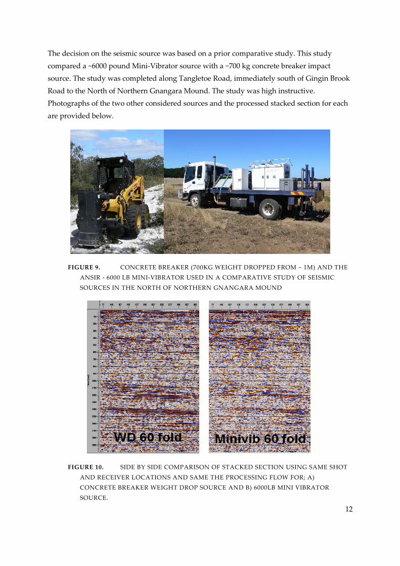
The decision on the seismic source was based on a prior comparative study. This study

compared a ~6000 pound Mini-Vibrator source with a ~700 kg concrete breaker impact

source. The study was completed along Tangletoe Road, immediately south of Gingin Brook

Road to the North of Northern Gnangara Mound. The study was high instructive.

Photographs of the two other considered sources and the processed stacked section for each

are provided below.

FIGURE 9. CONCRETE BREAKER (700KG WEIGHT DROPPED FROM ~ 1M) AND THE

ANSIR - 6000 LB MINI-VIBRATOR USED IN A COMPARATIVE STUDY OF SEISMIC

SOURCES IN THE NORTH OF NORTHERN GNANGARA MOUND

FIGURE 10. SIDE BY SIDE COMPARISON OF STACKED SECTION USING SAME SHOT

AND RECEIVER LOCATIONS AND SAME THE PROCESSING FLOW FOR; A)

CONCRETE BREAKER WEIGHT DROP SOURCE AND B) 6000LB MINI VIBRATOR

SOURCE.

13

GEOPHONES

The 2D seismic survey used 10 Hz geophones. The geophones were laboratory tested and

found to be linear in the range ~10 to ~400 Hz. This spans the range of “useful” frequency

content expected. That is, it is unlikely that frequencies content below 15 Hz or above 150 Hz

will be recoverable after processing. In short, 10 Hz geophones were considered to limit

frequency content of data acquired.

SEISMIC ACQUISITION SYSTEM

A new distributed-array Seistronix acquisition system was used for data collection. Refer to

the web site: http://www.seistronix.com/ for specification of the Seistronix EX6 system.

Photographs of an EX6 system truck line unit and tap unit are provided below along with an

"action" shot at a field data acquisition point.

FIGURE 11. THE IMAGES ABOVE SHOW A TRUNK LINE UNIT AND TAP UNIT FROM

THE SEISTRONIX EX6 SEISMIC ACQUISITION SYSTEM. SIXTY AU (ACQUISITION

UNIT) BOXES, EACH CAPABLE OF RECORDING 6 CHANNELS

14

SURVEY PARAMETER SETTING

All basic 2D seismic acquisition parameters were kept constant for the Tuart Road and

Clover Road surveys. The basic parameters used include:

Sample Rate = 1 msec

Trace length = 2.5 sec

Gain Setting = 24 dB

Pre-trigger = 10 msec

SURVEY GEOMETRY

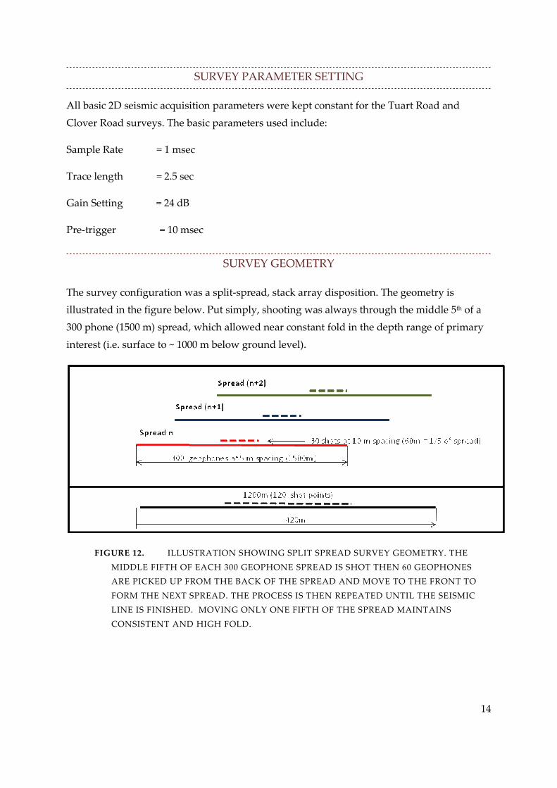
The survey configuration was a split-spread, stack array disposition. The geometry is

illustrated in the figure below. Put simply, shooting was always through the middle 5th of a

300 phone (1500 m) spread, which allowed near constant fold in the depth range of primary

interest (i.e. surface to ~ 1000 m below ground level).

FIGURE 12. ILLUSTRATION SHOWING SPLIT SPREAD SURVEY GEOMETRY. THE

MIDDLE FIFTH OF EACH 300 GEOPHONE SPREAD IS SHOT THEN 60 GEOPHONES

ARE PICKED UP FROM THE BACK OF THE SPREAD AND MOVE TO THE FRONT TO

FORM THE NEXT SPREAD. THE PROCESS IS THEN REPEATED UNTIL THE SEISMIC

LINE IS FINISHED. MOVING ONLY ONE FIFTH OF THE SPREAD MAINTAINS

CONSISTENT AND HIGH FOLD.

15

DATA ACQUIRED

The 2D seismic data sets acquired and detail concerning VSP, FWF sonic and Ground

Penetrating Radar equipment and acquisition are outlined below.

The geometry corrected SEGY shot records contain a complete record of survey geometry

and parameters. The detail will not be repeated here other than to provide the name and

basic details for each SEGY file for Tuart Road 3A, Tuart Road 3B and Clover Road

respectively. Details for the geometry of the stacked sections are provided in the processing

section of this report.

FIGURE 13. BASIC DATA FOR TUART ROAD TRANSECT 3A GEOMETRY CORRECTED

SHOT RECORD FILE.

FIGURE 14. BASIC DATA FOR TUART ROAD TRANSECT 3B GEOMETRY CORRECTED

SHOT RECORDS FILE.

16

FIGURE 15. BASIC DATA FOR CLOVER ROAD GEOMETRY CORRECTED SHOT

RECORD FILE.

VERTICAL SEISMIC PROFILING (VSP)

Vertical Seismic Profiling (VSP) data was collected with a 24-channel, hydrophone string

mounted in a 4WD off-road trailer as shown below. The hydrophone string was purchased

by Water Corporation of Western Australia to support research into VSP for hydrogeology.

The hydrophone string is some 1000 m long and has 24 hydrophones spaced at 10 m

intervals (i.e. over 230 m) at the bottom of the string.

Hydrophones must be submersed in water to function correctly and are highly sensitive at

wide range of frequencies (e.g. into the KHz range). A hammer source was more than

sufficient to obtain clear first breaks (i.e. first arrival travel times) throughout each of the

Department of Water bores surveyed.

VSP surveying was completed in DoW monitoring bores NG3A, NG8A, and NG10A. At

least 11 zero offset shot records were acquired at each drill hole. That is, at each bore hole the

24 channel hydrophone string was pulled up at 1 m intervals 11 times to get complete one

metre coverage (i.e. hydrophones at 240 positions) over a significant portions of each hole.

A patch box (designed at Curtin University) was used to distribute the 24 channels from the

hydrophone string into four Seistronix acquisition units. Each Seistronix acquisition unit can

acquire six channels of data.

17

The EX6 acquisition system survey parameters used include:

Sample Rate: 0.25 msec

Trace length: 2 seconds

Gain : 24 db

Pre-trigger : 4 msec

FIGURE 16. PHOTOGRAPH OF HYDROPHONE STRING USED FOR VSP SURVEYING.

NOTE THE SAFETY SWITCHES ETC.

An example of the VSP data acquired is provided below. The image shows the 11 shot

records collected at bore hole NG8A. There are 25 traces collected for each shot record. Note

that the 25th trace is obtained in a geophone places and the bores collar.

18

FIGURE 17. EXAMPLE SHOWING OF 11 VSP SHOT RECORDS FROM BORE HOLE

NG8A. TWENTY FOUR CHANNELS COME FROM THE HYDROPHONE STRING AND 1

CHANNEL (I.E. THE 25TH TRACE) COMES FROM A GEOPHONE AT THE COLLAR.

FULL WAVE FORM SONIC WIRELINE LOGGING

The objective of the FWF sonic logging was to obtain near complete acoustic characterization

of the shallow Yarragadee in the frequency range 500 Hz to 25000 Hz.

Repeat Full Wave Form (FWF) sonic wire line logs were completed in the cored drill hole

NG3. The location of this cored hole is critical in understanding the 3D framework of the

Northern Gnangara Mound (see DoW reports for bore logs and locations). NG3-cored hole is

a location (i.e. along Stewart Road) where the Leederville Formation appears to pinch out

and where the shallow Yarragadee Formation appears to be split into two seismically

different units (i.e. a low velocity and higher velocity unit). It is a key location for later

interpretation of the 2D seismic data.

Data was acquired with the Mount Sopris Instrument FWF sonic probe. See the web site;

http://www.mountsopris.com/ for details on this instrument. Data was collected at four center

frequencies including: 1 KHz, 3 KHz, 5 KHz and 15 KHz, with a four receiver, one

transmitter tool configuration. The 1 KHz, 3 KHz and 5 KHz data were acquired with 16

microsecond (usec) sampling over 4.2 msec and the 15 KHz data was collected with 8usec

sampling with a trace length of 2.2 msec. Data was collected at a broad range of centre

19

frequencies such that dispersion (in amplitude and velocity) in compressional and Stoneley

wave data could be analysed. The tool is illustrated in the photograph below.

FIGURE 18. FWF SONIC TOOL USED TO ACQUIRE FWF SONIC DATA AT NG3-CORED

HOLE. SPACING BETWEEN RECEIVERS IS 1 FT AND THE DISTANCE FROM THE

TRANSMITTER TO THE FIRST RECEIVER IS 3 FT.

An example of data obtained at the four center frequencies is illustrated below. It should be

noted that the response at each center frequency is relatively broad band (e.g. there is

considerable overlap in frequency content). Frequency content of the signal will be discussed

more in the processing section of this report.

20

FIGURE 19. EXAMPLE OF FWF SONIC DATA COLLECTED AT A SINGLE DEPTH

(71.5M) FOR FOUR DIFFERENT TRANSITION CENTRE FREQUENCIES (I.E. 1 KHZ, 3

KHZ, 5 KHZ AND 15 KHZ).

SHEAR COMPRESSIONAL WAVE MEASUREMENTS ON CORE

There are an exceedingly small number of cored holes drilled into the shallow sediments of

the Perth Basin. These sediments, in particular the superficial, Leederville and Yarragadee

formations store significant volumes of water and are utilized for potable water supply for

Perth.

A cored hole was drilled in the Northern Perth basin in January 2009. The core provided a

rare opportunity to study the geology, hydrogeology and petrophysics of sediments of the

Perth Basin in detail. There are three main motivations for completing a detailed study of the

petrophysics of the sediment from the North Perth Basin at core scale:

• Build relationships between petrophysical parameters and hydrogeological

parameters for better understanding and interpretation in the Perth Basin. Develop

the specific relationship between a core scale between geology, hydrogeology and

21

petrophysics, such that these relationships can be better understood and inferred

across a wider basin area.

• Build the relationship between P and S wave velocities and hydrogeology for

interpretation of 2D seismic data acquired in the Northern Gnangara Mound.

Develop the general relationship between P and S wave velocities and hydraulic

parameters at core scale such that hydrogeology can be interpreted from sonic logs

and 2D seismic data acquired across the Northern Gnangara Mound. That is, some

60 kms of detailed 2D seismic data has been acquired across the Northern Gnangara

Mound. This data is being used to develop the large scale hydrostratigraphic

framework of the North Gnangara Mound. This work requires the development of a

model relating the 2D seismic image to determine hydrogeological properties.

• Develop the technologies for measuring and/or computing both acoustic and

hydraulic parameters for shallow moderately to weakly consolidated sediment

samples for a range of confining and pore pressures. The properties of shallow

sediments (i.e. the upper 1000 m) are of the highest importance in hydrogeology;

however, these can be exceedingly difficult to measure/determine and are not well

studied. Of particular importance is the change in acoustic and hydraulic parameters

with changes confining and/or pore pressure in the near surface (e.g. how do the

hydraulic/acoustic properties of shallow sediments vary with depth of burial up to

~1000m). This area of research needs to be developed at all levels (i.e. equipment,

data acquisition and theoretical model development). The core recovered from NG8

provides the opportunity to advance the methods for empirically and theoretically

determining these important relationships.

An emphasis has been placed on quality and verification of results (measurements) rather

than throughput (i.e. number of tests completed).

All core handling and testing was completed by a commercial core laboratory. It was

assumed that standard 38 mm DIA plugs will be cut from frozen sandstone core samples

then mounted within a Teflon case. Unfortunately the core plugs that were recovered were

not of sufficient quality for testing. New plugs needed to be cut and this delayed recovery of

compressional and shear wave parameters. These tests will be completed later in 2009.

Careful attention will be paid to the validation and verification of results. To this end

verification of the measurements obtained at Curtin will be reviewed by two independent

research facilities, including UWA’s soft sediment laboratory. Bender testing has been

completed at UWA and examples of the resulting measurements are detailed below.

22

SHEAR WAVE MEASURMENTS (BENDER TESTS)

An essential component of recovering near complete acoustic characterization of the shallow

Yarragadee is recovery of shear waves. Shear wave cannot be obtained in-situ from the FWF

sonic logs with the MSI monopole logging system. This is because the shear wave is slower

than the bore hole fluid velocity. In this case, the shear wave velocity for specific lithologies

and depths can only be recovered by shear wave velocity measurements on core samples at a

range of confining/overburden pressures (i.e. effective pressures). Although the “Bender

Testing” is expensive, it is also likely that there will be no other opportunity to determine

this key acoustic parameter from the shallow Yarragadee in the near to medium term.

Five bender tests were completed on core samples obtained from the Shallow Yarragadee

from cored hole NG3.

The shear wave velocities versus effective pressure obtained for the five sandstone samples

are provided below. Complete Bender Test reports are available for each sample.

FIGURE 20. SHEAR WAVE VERSUS EFFECTIVE CELL PRESSURE FOR DEPTH

INTERVAL 64.6 – 64.78 (SAMPLE 1)

23


INTERVAL 170.1 – 170.3 (SAMPLE 2)


INTERVAL 145.3 – 145.6 – SAMPLE 3

24




INTERVAL 138.6-138.9 SAMPLE 5

25

FIGURE 25. QUALITY CONTROL TEST SHOWING SHEAR WAVE VERSUS CONSTANT

EFFECTIVE CELL PRESSURE FOR CHANGING PORE PRESSURE FOR DEPTH


COMPRESSIONAL WAVE MEASUREMENTS - NO CORE

Though not as critical as measuring shear wave velocity, the measurement of compressional

wave velocities is still important. The reason is that compressional wave velocities are

directly measured by the full-wave form, sonic wire-line logging. Shear wave velocities

cannot be recovered from such logging in low velocity sediments.

There has been considerable delay in the measurement of compression wave velocities for

the simple reason the core plugs supplied are not of sufficient quality to justify the time

consuming and expensive measurements. The picture below shows the state of plugs

supplied in black (from NG3) and compares to samples from a different core hole in the

Leederville formation. New plugs have recently been cut from the 5 whole core samples

supplied to UWA for Bender testing.

An additional four whole core samples were selected from the core that had been laid out at

the commercial laboratories. No sample supplied from the commercial laboratory could be

cut into standard 38mm diameter plugs. Only the samples preserved for Bender testing

could be cut and mounted as 38 mm plugs. The 38 mm core plugs have only recently been

cut and so are not included in this report.

26

FIGURE 26. EXAMPLE OF NG3 CORE PLUGS COMPARE TO CORE PLUGS FROM

WATER CORPORATIONS M345 SITE. CORE PLUGS FROM NG3 (I.E. THE TWO ON THE

LEFT) WERE NOT BELIEVED TO BE OF SUITABLE QUALITY FOR COMPRESSIONAL

AND SHEAR WAVE VERSUS CONFINING PRESSURE TESTS.

RADAR DATA ACQUISITION

Two Ground Penetrating Radar (GPR) transects were acquired along Tuart and Clover

Roads by Geoforce Pty Ltd. The data for Tuart and Clover Road is shown in the figures

below. The basic parameters for surveying were:

Trace Increment: 0.1m for Tuart Road and 0.05 m for Clover Road.

Number of Traces: 157815 for Tuart Road and 431211 for Clover Road

Time Increment: 0.4 nsec

Sample Number: 664 for Tuart Road, 1024 for Clover Road.

Source Receiver Separation – Distance: 0.35 m

Distance Method: Measurement Wheel 100 MHz = 3

Antenna: Mala 250 MHz Shielded

Nominal Frequency: 250 MHz

The two figures below illustrate the Ground Penetrating Data (GPR) acquired along Tuart

Road (~15 km) and Clover Road (~35 km).

27

FIGURE 27. RAW 250 MHZ RADAR DATA ACQUIRED ON TUART ROAD (MEAN

REMOVED / TRACE NORMALIZED)

FIGURE 28. RAW 250 MHZ RADAR DATA ACQUIRED ON CLOVER ROAD (MEAN

REMOVED / TRACE NORMALIZED)

28

PROCESSING

Processing of all data sets was completed in Reflexw (i.e. Radar) and/or Landmark PROMAX

(e.g. VSP, 2D seismic and FWF sonic). Processed data sets are provided in the table below.

Processed data is backed up on Curtin University computer system. Also data has been

made available to the Department of Water.

Survey Record Type

Number

of Records

File Type Containing

Record

Tuart Road Transect 3A

Stacked

Section 1

SEGY - Complete

Geometry

Tuart Road Transect 3B

Stacked

Section 1

SEGY - Complete

Geometry

Cover Road Transect 4

Stacked

Section 1

SEGY - Complete

Geometry

NG3A VSP Shot Records 11

SEGY - Complete

Geometry

NG8A

Shot Records

11

SEGY - Complete

Geometry

NG10A

Shot Records

22

SEGY - Complete

Geometry

NG3-cored hole FWF

sonic Velocities 4

ASCII

NG3A FWF sonic Velocities 1 ASCII

Tuart Road Radar

250MHz Line km ~15 ReflexW and SEGY

Clover Road Radar

250MHz Line km ~35 ReflexW and SEGY FIGURE 29. TABLE OF PROCESSED DATA SETS.

2D SEISMIC

Data acquisition was accomplished with a high-fidelity, 24-bit distributed telemetric

Seistronix system. A 1000 kg concrete breaker mounted on the front of a tracked bob cat was

used as seismic source.

Obtaining a high-resolution P-wave image was the primary interest for this investigation.

However, the ambient noise and deep, unconsolidated sand dunes and/or shallow limestone

can prevent generation of high quality, high-frequency seismic images. The Tuart and

Clover Road transects were processed as crooked lines. Velocity analysis was used, where

29

velocities were defined by examining either semblances, the flatness of NMO hyperbola or

partial stacks (see Appendix 1, Figure A4).

Recovering high resolution data from the very near surface unconsolidated superficial

sediments through to the highly variable Leederville Formation and into the Yarragadee

Formation was highly challenging and took longer than expected. Of particular importance

in the processing was refraction statics, deconvolution and velocity analysis.

The final processing flow carried out on the data is summarised below:

1. Recording geometry definition: straight + crooked track selection, binning along the track

at 5 m intervals, and QC-displays.

2. Trace edit: reverse.

3. First break picking (manual first break picking was required for al 3262 shot records)

4. First breaks editing and computation of refraction statics using DRM method.

5. Stack (Brute-1), single velocity function using “guide” function from constant velocity

stack panels.

6. Spectral analysis, deconvolution, band-pass filter tests, and multi-channel filter test.

7. Amplitude analysis: application of shot RMS energy equalisation, spherical divergence

correction, and reflection losses.

8. Application of spiking deconvolution

9. Band pass filter.

10. Surface wave noise attenuation using an apparent velocity.

11. CVS velocity analysis and NMO-I application.

12. Stack to Brute-2.

13. Deep move out corrections

14. CVS analysis II and NMO-II application

15. DMO stack

16. Final time stack

17. Time migration

18. Depth conversion

30

Many additional processing flows were attempted to improve the S/N ratio; however, no

significant improvements were achieved. Research into processing specific to hydrogeology

and shallow unconsolidated sediments (0 to 1000m) is ongoing with some aspects of this

area being the subject of a new PHD.

All processing flows are retained at Curtin University. All processed data sets are contained

within the Landmark PROMAX software package. It is important to note that PROMAX

retains a complete processing history. Data and processing flows are made available for

research at Curtin University’s Department of Explorations Geophysics. The data sets are

currently used by three PHD students and numerous masters and Honours students, who

have related research projects.

Of particular note in this project is the time and effort that when into first break picking. That

is, first breaks were picked by hand for every shot record (i.e. there are likely to be of the

order 1 million first break picks).

The two shot records below give some indication of the data quality obtained from the 2D

surveying. First breaks were in general well resolved along the full 1500m spread length,

however they were not consistent enough for automatic picking algorithms to generate a

satisfactory result.

FIGURE 30. EXAMPLE OF A SHOT RECORD FROM START OF CLOVER ROAD.

EXAMPLE IS FOR SHOT EIGHTEEN ON THE FIRST SPREAD (SHOOTING INTO THE

FIRST SPREAD ALONG CLOVER ROAD).

31

FIGURE 31. EXAMPLE OF A SHOT RECORD FROM THE SECOND SPREAD ALONG

CLOVER ROAD (BAD TRACES HAVE BEEN REMOVED).

A brief review of data coverage, quality and processing for each transect is provided below.

TUART ROAD – 3A

The image below shows the geometry of the Tuart Road 3A transect. The color bar to the left

indicates the range of elevations along the road. Note that the northing direction is

exaggerated and the Tuart Road transect is relatively straight in the East West direction.

FIGURE 32. MAP SHOWING SIN_Y_COORD AND SIN_X_COORD AND ELEVATION

GEOMETRY FOR THE TUART ROAD 3A TRANSECT.

32

The figure below shows a stacking chart. The main point from the diagram below is that fold

is relatively high (e.g. greater than 80) and uniform.

FIGURE 33. 2D STACKING CHART FOR THE TUART ROAD 3A TRANSECT.

The figure below shows elevations plotted against Easting with the total static correction

indicated in the colour range blue to red. Maximum static correction was close to 120 msec at

the highest elevation towards the west of the line.

FIGURE 34. TUART ROAD 3A CDP ELEVATION AND C-STATIC CORRECTION.

As a general comment processing became difficult towards the western end of Tuart Road

3A. Problems related to more rapid changes in velocity and a complex velocity structure in

the near surface. That is a complex arrangement of near surface limestone and

unconsolidated sand units made removal of statics difficult. Processing to reduce these

problems is ongoing; however, on the whole (e.g. excluding the west of the line) the quality

of the processed stacked section was excellent.

TUART ROAD – 3B

Tuart Road 3B extended the Tuart Road 3A coverage to the west of Wanneroo Road by about

3 km. The transect remains East-West in orientation. The figure below shows CDP elevation

33

against Easting with CDP fold indicated as color on the right hand colour bar. Fold remained

above 80 for most of the line. To ensure some overlap with Tuart Road 3B, shooting started

to East of Wanneroo Road. The Tuart Road 3B geophones were placed immediately to the

West of Wanneroo Road (a major Road) and source points started on the East of Wanneroo

Road (~400 to the East of the First Geophone). The highest fold (>150) is obtained as the shot

points move into the first spread going west.

FIGURE 35. FOLD GEOMETRY AND ELEVATION ALONG TUART ROAD 3B

CLOVER ROAD

Clover Road was the longest transect. The image below shows Northing mapped against

Easting with CDP fold shown in the color range blue to red. Again CDP fold was high and

relatively constant throughout the line. The approximately 18 km long line clearly changes

direction such that application of crooked line processing was essential.

FIGURE 36. MAP OF CDP_X AND CDP_Y SHOWING FOLD GEOMETRY ALONG LINE.

The image below is a trace midpoint map for clover road. It shows that the bends in Clover

Road are relatively benign and prose no serious problem to processing if crooked line

processing is used correctly.

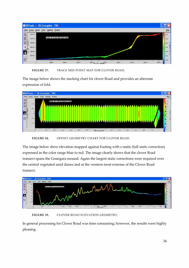
34

FIGURE 37. TRACE MID-POINT MAP FOR CLOVER ROAD.

The image below shows the stacking chart for clover Road and provides an alternate

expression of fold.

FIGURE 38. OFFSET GEOMETRY CHART FOR CLOVER ROAD.

The image below show elevation mapped against Easting with c-static (full static correction)

expressed in the color range blue to red. The image clearly shows that the clover Road

transect spans the Gnangara mound. Again the largest static corrections were required over

the central vegetated sand dunes and at the western most extreme of the Clover Road

transect.

FIGURE 39. CLOVER ROAD ELEVATION GEOMETRY.

In general processing for Clover Road was time consuming; however, the results were highly

pleasing.

35

STACKED SECTIONS

Some examples of stacks sections are provided to illustrate data quality and any processing

problems that occurred. In general, quality of the processed stacked data was excellent. Final

imaging and interpretation will be completed in a later research phase.

TUART ROAD – 3A

The stacked section and migrated stacked sections for the Tuart Road 3A show the key

contact between the Leederville and Yarragadee Formations being clear in both images (i.e.

the unconformity between flat lying and dipping beds).

FIGURE 40. STACKED SECTION FOR TUART ROAD 3A PRIOR TO MIGRATION.

FIGURE 41. STACKED SECTION FOR TUART ROAD 3A AFTER MIGRATION

36

FIGURE 42. EXAMPLE OF DATA QUALITY ALONG A 4.5 KM LENGTH OF THE TUART

ROAD 3A 2D SEISMIC TRANSECT. NOTE THE CLEAR UNCONFORMITY BETWEEN

FLAT LYING (LEEDERVILLE) AND DIPPING (YARRAGADEE) LAYERS.

The eastern most end of Tuart Road 3A was completed with a ~ 2km overlap of the existing

transect. The overlapping survey crosses a complex fault zone. The existing transect was

completed with a smaller source (650kg concrete breaker) and higher resolution survey

parameters. That is, the existing survey was completed with 4 m geophone spacing, 8 m shot

spacing and 0.5 msec sample rate.

Both surveys provided an excellent image of the complex fault zone and as expected higher

resolution data was obtain with higher spatial and temporal sampling, while greater depth

of penetration was obtained with the larger weight drop source. More detail comparison is

proceeding as ongoing research.

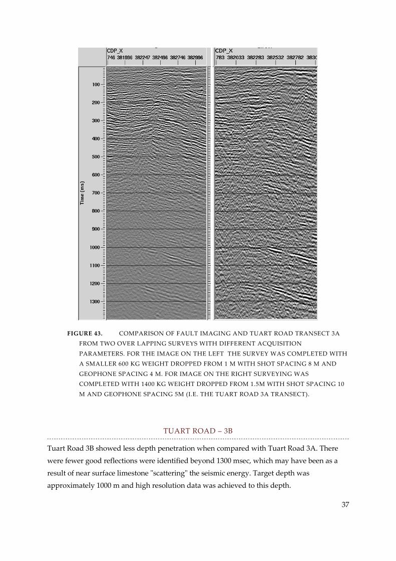
37

FIGURE 43. COMPARISON OF FAULT IMAGING AND TUART ROAD TRANSECT 3A

FROM TWO OVER LAPPING SURVEYS WITH DIFFERENT ACQUISITION

PARAMETERS. FOR THE IMAGE ON THE LEFT THE SURVEY WAS COMPLETED WITH

A SMALLER 600 KG WEIGHT DROPPED FROM 1 M WITH SHOT SPACING 8 M AND

GEOPHONE SPACING 4 M. FOR IMAGE ON THE RIGHT SURVEYING WAS

COMPLETED WITH 1400 KG WEIGHT DROPPED FROM 1.5M WITH SHOT SPACING 10

M AND GEOPHONE SPACING 5M (I.E. THE TUART ROAD 3A TRANSECT).

TUART ROAD – 3B

Tuart Road 3B showed less depth penetration when compared with Tuart Road 3A. There

were fewer good reflections were identified beyond 1300 msec, which may have been as a

result of near surface limestone "scattering" the seismic energy. Target depth was

approximately 1000 m and high resolution data was achieved to this depth.

38

FIGURE 44. EXAMPLE OF MIGRATED STACKED SECTION FOR TUART ROAD

TRANSECT 3B PLOTTED AGAINST EASTING.

Again migration smiles are apparent in the above image. There are several cosmetic

processing steps to remove these. These may be applied to the post stack data at a later date.

CLOVER ROAD

The very long Clover Road transect is perhaps the most pleasing result. The unconformity

between Leederville and Yarragadee is exceedingly well resolved and the definition within

the Yarragadee is exceptional.

FIGURE 45. EXAMPLE OF STACKED SECTION FOR TUART ROAD TRANSECT 3B

PLOTTED AGAINST EASTING. THE TRANSECT IS MORE THAN 18 KM LONG.

39

An additional image is provided below to illustrate data quality.

FIGURE 46. EXAMPLE OF STACKED AND MIGRATED SECTION FOR TUART ROAD

TRANSECT 3B PLOTTED AGAINST EASTING. NOTE THE VERY HIGH RESOLUTION

FROM SURFACE TO 1500 MSEC.

The most pleasing outcome from the 2D seismic, as illustrated in the above examples, is that

high resolution was maintained from surface to ~1500 msec. In particular the resolution of

shallow layers is important, if the hydraulic relationships between superficial, Leederville

and Yarragadee formations are to be revealed.

ALL STACKED SECTIONS

The Clover Road and Tuart Road 2D Seismic transects significantly increase the span of

existing 2D seismic surveys in the Yeal area. In the image below the existing surveys are

shown blanked out (i.e. white sections). These blanked out sections were commissioned by

the Water Corporation of Western Australia. Data sharing agreements are in place such that

a near complete picture of the stratigraphy of the Northern Gnangara Mound can now be

developed. These three images below illustrate the locations the processed 2D Seismic

stacked sections.

40

FIGURE 47. DEPARTMENT OF WATER STACKED SECTIONS FOR TUART ROAD

TRANSECT 3A, TUART ROAD 3B AND CLOVER ROAD WITHIN A 3D VOLUME.

TRANSECT BLANKED AS WHITE ARE PRE-EXISTING HIGH RESOLUTION 2D SEISMIC

DATA ACQUIRED FOR WATER CORPORATION OF WESTERN AUSTRALIA.


AND CLOVER ROAD WITHIN A 3D VOLUME. TRANSECT BLANKED AS WHITE ARE

PRE-EXISTING HIGH RESOLUTION 2D SEISMIC DATA ACQUIRED FOR WATER

CORPORATION OF WESTERN AUSTRALIA. IMAGE ALSO SHOWS INDICATES THE

LOCATION SPARSE MONITORING BORES (I.E. WIRE LINE LOGS – GAMMA RED AND

SHORT NORMAL BLUE).

41

FIGURE 49. STACKED SECTION FOR CLOVER ROAD WITHIN A 3D VOLUME

LOOKING FROM THE EAST (I.E. BRAND HWY) TOWAROADS THE WEST.

VSP AND WIRE-LINE LOGGING

Comprehensive Full Wave Form (FWF) sonic logging has been completed in the Department

of Water’s cored hole NG3. Vertical Seismic Profiling (VSP) was also completed in the

finalised Department of Water monitoring bores NG3A, NG8A and NG10A. The purpose of

the survey was to provide:

a) clear acoustic characterization of the three major formations (i.e. the Superficial

Formation, the Leederville Formation, and the Yarragadee Formation) such that 2D

sections could be tied into the key formations (i.e. time to depth conversion, and

acoustic impedance distribution), and

b) high quality data sets for ongoing research programs into the seismic methods,

hydrogeology and hydrogeophysics.

VSP

The zero offset VSP data was obtained with a 24 channel hydrophone string. The survey

parameters for the zero offset VSP survey are provided in the table below. Ten blows with

the sledge hammer source were stacked for each shot record. Twenty five channels of data

were recorded. Twenty four channels came from the hydrophone string and the twenty fifth

42

recording channel was an input from a geophone planted in the ground at the top of the

bore.

FIGURE 50. ACQUISITION PARAMETERS FOR ZERO OFFSET VSP SURVEYING AT

MONITORING BORE NG8A, NG3A, AND NG10A.

The example below shows 1 of the 11 zero offset VSP shot records completed at monitoring

bore NG8A. The first 3 channels were above the watertable and the 25th channel come from

the geophone planted near the top of the drill hole. The data quality is excellent. As expected

for a zero offset VSP with a hydrophone string tube, the response waves are strong.

FIGURE 51. EXAMPLE OF ZERO OFFSET VSP SHOT RECORD IN MONITORING BORE

NG8A. IMAGE SHOWS HYDROPHONE CHANNELS 1 TO 24, WITH THE 25TH CHANNEL

BEING A GEOPHONE AT THE SURFACE NEAR THE WELL COLLAR. NOTE THAT

SHOT RECORDS HAVE BEEN NORMALIZED.

Type of survey: Zero-offset VSP Energy source: Sledge Hammer / metal plate

Number of shots: 11 (minimum) Receivers: Hydrophones

Number of Channels: 24 Channel spacing: 10

Sample rate: 0.25 ms Trace length: 2000 ms

Gain : 24 db Pre-trigger: 4 ms

Number of Stacks 10 (blows with the Hammer = 1 shot)

43

VSP SURVEYING IN BORE NG3A

An example (i.e. 1 of 11 VSP records at NG3A) of a zero offset VSP shot record at NG3A is

provided below. The example shows a full shot record plotted with no scaling. Channels 1

and 2 are above the watertable. Again tube wave is clear in the full record.

FIGURE 52. EXAMPLE OF ZERO OFFSET VSP SHOT RECORD IN BORE NG3A. IMAGE

SHOWS HYDROPHONE CHANNELS 1 TO 24, WITH THE 25TH CHANNEL BEING A

GEOPHONE AT THE SURFACE NEAR THE WELL COLLAR.

The figure below shows a complete zero offset shot record for NG3A zoomed to the first

breaks. The first break data is clear and drop off in amplitude is broadly consistent with

spherical spreading. Again the tube waves follow closely behind the first arrivals.

FIGURE 53. EXAMPLE OF ZERO OFFSET VSP SHOT RECORD (IN THE TIME RANGE 0

TO 160MSEC) IN BORE NG3A. IMAGE SHOWS HYDROPHONE CHANNELS 1 TO 24,

WITH THE 25TH CHANNEL BEING A GEOPHONE AT THE SURFACE NEAR THE WELL

COLLAR.

44


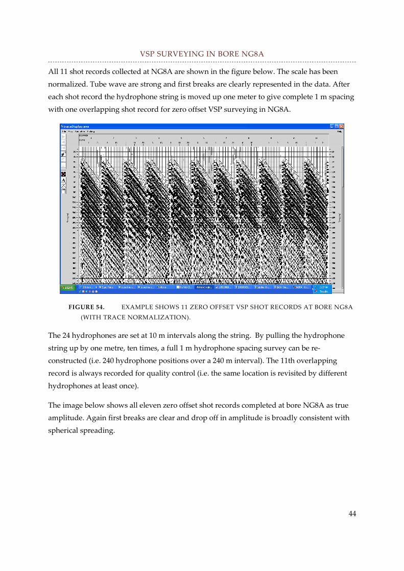
All 11 shot records collected at NG8A are shown in the figure below. The scale has been

normalized. Tube wave are strong and first breaks are clearly represented in the data. After

each shot record the hydrophone string is moved up one meter to give complete 1 m spacing

with one overlapping shot record for zero offset VSP surveying in NG8A.


(WITH TRACE NORMALIZATION).

The 24 hydrophones are set at 10 m intervals along the string. By pulling the hydrophone

string up by one metre, ten times, a full 1 m hydrophone spacing survey can be re-

constructed (i.e. 240 hydrophone positions over a 240 m interval). The 11th overlapping

record is always recorded for quality control (i.e. the same location is revisited by different

hydrophones at least once).

The image below shows all eleven zero offset shot records completed at bore NG8A as true

amplitude. Again first breaks are clear and drop off in amplitude is broadly consistent with

spherical spreading.

45


(NO SCALING).


The example below from Department of Water (DoW) monitoring Bore Hole NG10A

illustrates a full shot record showing the depth for each trace along the horizontal axis (e.g.

depth below ground level for each hydrophone is shown on the horizontal axis). All data is

depth corrected. Twenty two zero offset VSP surveys were collected in bore hole NG10A.

Eleven were completed with the string moved down 1 m after every shot in the depth

interval 10 and 20 m inclusive.

Eleven additional VSP surveys were completed with the hydrophone string moved after

every shot by 1 m in the interval 50 to 60m. That is, the upper hydrophone was moved

inward at one metre increment s after each shot record in the interval 50 and 60 m below

ground level. The shot record at with the upper hydrophone located at 50m is shown below.

First breaks were picked for all shot records to provide detailed time to depth information.

The blue and red line in the figure below illustrates first break picking based on zero cross

over (red picks) and peak amplitude (blue picks) respectively. Generally speaking the first

break down (i.e. red crosses) is considered to be “correct” method for first break picking. It is

however necessary to check the consistency of first break picking against peak amplitude

picking, which is faster and often more robust if amplitudes of the first break down become

very small.

46

FIGURE 56. EXAMPLE OF A FULL ZERO OFFSET VSP SHOT RECORDS WITH THE

UPPER HYDROPHONE LOCATED AT BORE NG10A (NO SCALING APPLIED).

FIGURE 57. EXAMPLE OF ZERO OFFSET VSP FIRST BREAK PICKING AT NG10A

PLOTTED AGAINST DEPTH. VERY ACCURATE PICKING OF FIRST BREAK CAN BE

HIGHLY CHALLENGING WHERE AMPLITUDES OF THE FIRST BREAK DOWN

BECOME SMALL.

47

The figure below illustrates a combined plot of 10 shot records completed where the

hydrophone string is more down at 1m intervals such that the upper hydrophone is located

at 50, 51,52 … 58, 59 and 60 m. Data is sort by depth such that the end result is a highly

detailed shot composite shot record with 240 traces over 240m as show below.

FIGURE 58. EXAMPLE OF COMBINATION OF 10 ZERO OFFSET VSP SHOT RECORDS

SORTED BY DEPTH IN BORE NG10A. BY COMBINING 10 SHOT RECORD EACH

COMPLETED WITH THE 24 HYDROPHONES STRING (I.E. 10 M SPACING) A DETAILED

SHOT RECORD WITH 240 HYDROPHONE POSITIONS CAN BE RECONSTRUCTED.

NOTE THE STRONG TUBE WAVES IN THIS AND ALL ZERO OFFSET VSP

HYDROPHONE STRING RECORDS.

It was not the intention of this report to explain ongoing detailed research programs.

However, one example of a zero-offset VSP corridor stack generated from a shot record at

NG10A is shown below. Note that every shot record (i.e. there are 22 shot records at NG10A)

will generate a similar zero-offset VSP corridor stack. The advanced processing is completed

by Assoc. Prof. Roman Pevzner who is trialing a range of methods for VSP processing, in

particular methods for tube wave suppression.

48

FIGURE 59. EXAMPLE OF DEPTH CONVERTED CORRIDOR STACK FOR ONE ZERO

OFFSET VSP AT NG10A (LEFT) COMPARED TO STACKED DEPTH CONVERTED 2D

SEISMIC TRACES AT THE SAME LOCATION. THE ZERO OFFSET VSP PROVIDES ARE

ROBUST REPRESENTATION OF THE ACOUSTIC IMPEDANCE DISTRIBUTION AT A

SPECIFIC BORE LOCATION. THE TWO 2D SEISMIC DATA IS NOT EXPECTED TO

MATCH EXACTLY, HOWEVER THE BASIC CORRELATION IS HIGHLY PLEASING.

49

WIRELINE LOGGING

A comprehensive suite of FWF Sonic Wire Line Logs were collected immediately on

completion of drilling NG3-core hole. A four receiver, one transmitter, monopole Mound

Sopris Instruments (MSI) tool was used for logging. Logging was completed at four

transmitter centre frequencies including 1, 3, 5 and 15 KHz. All four frequencies were

acquired in the key depth range from 55 to 87 m. FWF sonic logs at 1 and 15 KHz were

completed over the full depth interval (~0 to 200m). The wire line log data was converted to

SEGY format and imported into PROMAX (seismic processing software). The figure below

illustrated all data acquired in the depth range 55 to 87 m. That is Rx1, Rx2, Rx3 and Rx4 for

the interval 55 to 87 m is shown for transmitter centre frequencies 1, 3, 5, and 15 KHz.

FIGURE 60. EXAMPLE OF FWF SONIC IMPORTED IN PROMAX FOR ANALYSIS.

FIGURE SHOWS 16 DATA SETS ALL IN THE DEPTH RANGE 55 TO 87 M. DATA SETS

ARE SORTED BY TRANSMITTER(TX) CENTRE FREQUENCY (I.E. 1, 3, 5 AND 15 KHZ)

THEN BE RECEIVER (RX) NUMBER (RX1, RX2, RX3, AND RX4). TRANSMITTER

RECEIVER SEPARATIONS ARE TX1RX1=3 FT, TX1RX2=4FT, TX1RX3=5FT, AND

TX1RX4=6FT.

It should be noted that even with transmitter centre frequency set to 1 KHz energy exists

across a relatively wide spectral range. The spectral energy can be illustrated by applying

spectral analysis to the received traces as shown below.

50

FIGURE 61. EXAMPLE OF SPECTRAL ANALYSIS OF TRACE AT 82.2M AND 81.4 M.

TRACES WERE RECORDED IN RECEIVER RX1 USING TRANSMISSION CENTRE

FREQUENCIES OF 1KHZ AND 3 KHZ HZ RESPECTIVELY.

The figure below illustrated the 3 KHz transmitter centre frequency FWF sonic data for Rx1,

Rx2, Rx3 and Rx4 for the depth interval 55 to 87m. First arrival of the “compressional wave”

is clear. However the stoneley wave is also very clear in particular at deeper 1/3 of the log.

A first pass attempt to recover change in compressional wave velocity with frequency was

made. This involves a triangular band pass filter with the shape “1KHz-3KHz-3Hz-6KHz”

being applied to the 3 KHz transmitter center frequency data with velocities recovered

between Rx1 and Rx3. Next a band pass filter with shape “10Khz-15KHz-15KHz-30KHz”

was applied to the 15 KHz transmitter center frequency data and velocities recovered

between Rx1 and Rx3.

51

FIGURE 62. EXAMPLE OF FWF SONIC RESPONSE WITH DEPTH FOR RX1, RX2, RX3

AND RX4 FOR TRANSMITTER CENTER FREQUENCY 3 KHZ.

The figure below illustrates first break picking for the 3 KHz filtered data (blue line) and 15

KHz filtered data (red line). Note that it is the separation between Rx1 and Rx3 (i.e. 2 ft) and

the difference in travel time between Rx1 and Rx3 that defines the velocities. Velocity is not

defined by total travel times which is more strongly affected by exactly how first break

picking has been completed.

FIGURE 63. EXAMPLE OF VELOCITY PICKING FOR 15 KHZ FWF SONIC DATA. RED

LINE IS FIRST BREAK PICK FOR 15 KHZ TRANSMITTER CENTRE FREQUENCY AND

BLUE LINE IS FIRST BREAK PICK FOR 3 KHZ TRANSMITTER CENTRE FREQUENCY.

52

The next figure illustrates velocity determined from the filtered 15 KHz data and filtered 3

KHz data, as well as the percent difference between the 15 KHz data and 3 KHz data. The

plot of percent difference can be considered “pseudo-dispersion” in velocity. These curves

certainly cannot be regarded as a mapping of dispersion but rather provide an indication of

which lithologies may be more "dispersive" over the selected frequency range.

Of particular note is the interval between 68 and 72 m showing the highest velocity

difference between 3 and 15 KHz. This interval is known to be unconsolidated course

grained sand/gravel (up to 5mm grain size) and most of the interval could not be recovered

as core (i.e. the core was lost during drilling). Research is proceeding into robust methods of

recovering velocity dispersion with frequency and amplitude from multi-frequency data

sets.

In addition to analysis of compressional wave velocity, stoneley waves (i.e. a type of tube

wave) are well recognized within the low frequency FWF sonic data sets. The figure below

shows Stoneley wave velocities derived from the 1 KHz transmitter centre frequency data

set. The Stoneley wave velocity can be revealed by first low pass filtering then using

standard semblance analysis.

We see a sharp increase in Stoneley wave velocity at 76 m depth below ground level. The

Stoneley wave velocities strongly characterized a key interface in Yarragadee formation. This

interface is not recognized in gamma or resistivity logs. Compressional and Stoneley wave

velocity logs proved to be the only robust way to identify a significant acoustic/stratigraphic

boundary at cored hole NG3. If the FWF sonic can be shown to be effective in cased holes

(early test indicate this will be possible) then this important interface can be mapped

throughout the area (note it is expected that only compressional wave can be detected

through FRP casing).

53

FIGURE 64. PROCESSED FILTERED FWF SONIC 15 KHZ TRANSMITTER CENTRE

FREQUENCY AND FILTERED 3 KHZ TRANSMITTER FREQUENCY “COMPRESSIONAL”

WAVE VELOCITIES ALONG WITH A “PSEUDO DISPERSION” CURVE.

54

FIGURE 65. STONELEY WAVE VELOCITIES RECOVERED FROM FILTERED 1 KHZ

CENTRE FREQUENCY FWF SONIC LOGGING. THERE IS A SIGNIFICANT BOUNDARY

AT ~76M. TWO VELOCITY RANGES ARE PROVIDED TO ILLUSTRATE THE LARGE

CHANGES IN STONELEY WAVE VELOCITY.

55

NG3 – BENDER TEST DATA ANALYSIS

Bender Test (including shear wave velocities) data is invaluable for a full analysis of the

acoustic properties of the Yarragadee Formation. These tests provide empirical data on

formation properties and create a basis for higher level research. This high quality Bender

test data can only be obtained from large diameter core and must be obtained soon after

drilling. Research into the mechanical properties of the Yarragadee and FWF sonic (in

particular Stoneley waves) are dependent on supporting evidence from bender testing on the

large diameter core samples.

The five curve below show shear wave velocities for five sandstone samples taken from the

indicated depths. The effective pressure can be related to depth of burial. The range of

effective pressures between 50 to 2500KPa can be broadly related to the first 200 m below

ground level. The figure shows the dramatic increase in shear wave velocity from below

150 m/sec at about 50KPa to more than 400 m/sec at 2500 KPa. The range of velocities at 2500

KPa (i.e. for samples 1 to 5) is between about 400 and 540 m/sec. This illustrates the

importance of confining pressure when considering the physical properties of rock in the

near surface.

FIGURE 66. SHEAR WAVE VELOCITY VS EFFECTIVE CELL PRESSURE FOR FIVE CORE

SAMPLE OBTAINED FROM CORED HOLE NG3. NOTE THAT THE CORE SAMPLES

FROM NG3 AT 64.6 AND 76.3 HAVE SIGNIFICANTLY LOWER SHEAR VELOCITY. THIS

IS CONSISTENT WITH FWF SONIC LOGGING.

56

FIGURE 67. SHEAR WAVE VELOCITY VERSUS EFFECTIVE CELL PRESSURE FOR FIVE

CORE SAMPLE OBTAINED FROM CORE HOLE NG3 SHOWN IN THE RANGE FROM 0

TO 10000 KPA EFFECTIVE CELL PRESSURE.

The chart below shows the range of shear velocities and shear modulous for the five

sandstone samples at an effective cell pressure of 1000 KPa (e.g. 1MPa).

FIGURE 68. COMPARISON OF SHEAR WAVE VELOCITIES AT 1000 KPA EFFECTIVE

PRESSURE

57

COMPRESSIONAL AND SHEAR WAVE MEASUREMENTS ON CORE

It was the intention to measure both compressional and shear wave velocities on standard

38mm core plugs after permeability and porosity measurements before 30 October 2009. The

objective of measuring compressional and shear waves was to characterize the acoustic

properties of the shallow Yarragadee formation at high frequencies (i.e. ultrasonic

frequencies). Accurate measurement of compression and shear wave velocities at different

effective pressure at ultra sonic frequencies for these shallow sand/sandstones will aid in:

• understanding the mechanical properties of the shallow Yarragadee,

• putting an upper limit on velocity dispersion with frequency, and

• determining, how acoustic properties (and mechanical properties) change with depth

of burial (e.g. dipping geological units in the Yarragadee can be mapped from surface

to hundreds or thousands of meters below surface).

Unfortunately the length of plugs was generally less than 4.5 cm and the quality of 38mm

plugs was exceedingly poor. It was not believed the research quality results could be

achieved with the supplied plugs. New plugs had to be cut for relatively time

consuming/expensive tests. As a result, new longer 38 mm DIA plugs have recently been cut

from the same five whole core samples used in Bender Testing at UWA. Of the five samples,

four high quality 6 cm long plugs have been recovered. It should be noted that several other

whole core samples were selected from core storage trays; however, no intact 38 mm plugs

could be recovered from the stored core samples suggesting that core preservation is critical.

Compressional and Shear wave testing will be completed in November to December 2009.

In conclusion, weakly consolidated sandstone is exceedingly difficult to handle requiring

samples to be immediately wrapped and preserved. Only these samples for Bender Testing

remained suitable for cutting of 6 cm plugs for compressional and shear wave ultrasonic

testing at a range of effective pressures.

58

GROUND PENETRATING RADAR

There are many elements to developing a groundwater flow model. Two of the most basic

elements are:

1. Hydraulic conductivity distribution (e.g. the general framework is nicely expressed in

the 2D seismic)

2. Recharge distribution.

The 2D seismic has been utilised to gain the general hydraulic framework and spatial

awareness of the Northern Gnangara Mound. With respect to better understand and define

recharge distribution, it is considered that Radar is more useful. In particular, as Ground

Penetrating Radar can express the difference between:

1. sand

2. clay

3. limestone and,

4. various water retentive layers: These are layers that retard the vertical progress of

water. They typically exist above the regional watertable in the superficial formation.

Data acquisition for Radar was completed along two long transects related to Tuart and

Clover Roads. The Department of Water radar data concentrates on resolving recharge

distribution in the Northern Gnangara mound. The Tuart Road and Clover Road transects fit

within a much wider program of Radar acquisition (i.e. some 400 km of Radar data has been

collected) that cover a large portion of the Gnangara Mound and is designed to resolve

recharge distribution over ~ 1000 square km. The wider GPR program was commissioned by

Water Corporation of Western Australia.

The location of the two transects within the Northern Gnangara Mound are located within

the 3D land surface image below.

59

FIGURE 69. LOCATION OF TUART ROAD AND CLOVER ROAD GPR TRANSECTS

LOCATED IN 3D. THE TUART ROAD TRANSECT IS LOCATED TO ABOUT 5KM TO THE

NORTH OF CLOVER ROAD.

TUART ROAD TRANSECT 3A AND 3B + EXTENSION

The depth corrected Tuart Road 250 MHz Radar section is illustrated below. The section is ~

15.5 km long with trace spacing about 10 cm, as such the figure below can only provide a

broad indication of data quality. Although not the intent of this document to provide

interpretations; however, the data shows the transition from patchy shallow reflectors and a

clear watertable as a single clear shallow reflector in the east.

FIGURE 70. EXAMPLE OF ~ 15KMS OF PROCESSED TUART ROAD RADAR DATA

60

The next two figures show higher resolution 250 MHz GPR data for Tuart Road, which

demonstrate good data quality. Each figure shows structure below the vegetated sand dunes

being resolved along with layers above, at and below the watertable itself.

FIGURE 71. EXAMPLE FOR ~100M OF PROCESSED TUART ROAD GPR DATA SHOWS

GPR DATA QUALITY.

FIGURE 72. EXAMPLE OF ~25 M OF PROCESSED TUART ROAD RADAR DATA

61

CLOVER ROAD, TRANSECT 4

As with the 2D seismic data, the 250 MHz radar transect along Clover Road is of high

quality. The east to west extent of the Gnangara Mound is almost completely surveyed by

the Clover Road transect. The presence of a strong shallow reflector in the east.

FIGURE 73. EXAMPLE OF ~21 KMS OF PROCESSED CLOVER ROAD GROUND

PENETRATING RADAR (GPR) DATA. AS WITH THE TUART ROAD, GPR DATA ALONG

CLOVER ROAD IS GOOD.

62

CONCLUSIONS

This report spans the acquisition and processing of geophysical data sets along Tuart Road

and Clover Road in the Northern Gnangara Mound for the Department of Water. It does not

provide detailed interpretations or new research topics, as this work is still ongoing.

Field conditions were challenging; however, all data sets were collected without incident.

All data sets are backed up at Curtin University’s Department of Exploration Geophysics

and have been made available to DoW. As improvements are made (e.g. improved

processing), any updated processed data sets are provided.

The objectives of the geophysics surveys in the Northern Gnangara Mound were:

a) to collect high quality geophysical data sets that may be used to interpret the

complex and important hydrogeological framework of the Northern

Gnangara Mound and,

b) to obtain data sets that will stimulate new insight and research activity in both

hydrogeology and geophysics.

It is considered that the objectives have been achieved. The framework and

hydrostratigraphic complexity of the top 1000 m of Northern Gnangara Mound has been

captured in the 2D seismic data. There is further detail and higher resolution that has been

detected in the top 20 m of the soil profile from the 250 MHz Radar. Vertical Seismic

Profiling, Full-Wave Form sonic, and core analysis has provided important support data for

understanding and interpreting the 2D seismic. This data was important for developing the

application of acoustic methods in hydrogeology.

Numerous research activities have been stimulated by the detailed geophysical acquisition

work completed within the Northern Gnangara Mound for DoW. A large numbers of

undergraduate have been exposed to hydrogeophysics. For example the 2008 Curtin

Geophysics third year field trip was to the Northern Gnangara Mound and included five

staff and nearly 30 students.

At present, there are two PHD students and three Honours students doing independent

research related into acoustic and electromagnetic methods in the Perth Basin. This number

is expected to increase in 2010 and 2011. Research into hydrogeophysics in Western Australia

has evolved rapidly over the past three years to become one of the most active programs in

the application of seismic and ground penetrating radar methods for hydrogeology in the

world.

63

APPENDIX 1: SEISMIC DATA PROCESSING - OVERVIEW

The notes below have been compiled by Milovan Urosevic and provide a general

explanation of many of the core 2D seismic processing steps completed for Tuart and

Clover Road Transects. Examples may not be from Tuart or Clover Road.

_______________________________________________________________________________

Processing of seismic reflection data involves numerous mathematical operations. Those can

be however grouped into three main categories:

I. Time corrections

II. Signal to noise improvement

III. Repositioning or inverse modeling

Time corrections involve:

a) Static corrections which aim to equalise travel times through typically low velocity

near surface weathered layer or so-called regolith in hard-rock environment. For this

computation we utilise waves which totally refract at the weathering/fresh rock

interface. This wave is a “diving” wave (Figure A1). For land seismic data this step is

of crucial importance since time delays through the regolith layer could completely

misalign reflected signals and result in destructive summation during the process of

stacking. Computed refraction statics cannot however fully compensate the travel

time differences through the weathered layer (regolith) due to the nature of head

waves which are “diving” through highly rugose intervals (Figure A1). Consequently

additional computations are required to fine-tune reflection events.

b) Residual statics. Those are conventionally computed using reflection events, again in

a surface consistent manner. We can also use here a modified procedure, which we

developed recently for the case of a low fold data and very week signal. The

procedure consists of the following steps:

- Time correct refracted events using linear equation (linear moveout or LMO)

with a velocity of the fresh rock derived under step a).

- Sort and stack refraction events.

64

- Pick horizon along refractions and select time window that encompasses only

refracted events.

- Compute residual statics using the algorithm devised for reflection data.

c) Dynamic corrections involve flattening reflection hyperbolae with appropriate

velocity (NMO velocity for short offset) in preparation for data summation (Figure

A2 and A3). The correction is based on the travel time equation (Figure A2) which is

derived for a single layer, constant velocity case. The same equation is valid for a

multi layer case as long as they are horizontal. The actual correction is implemented

on a sample by sample basis using the normal-move-out (NMO) equation (Figure

3A). Before this step can be carried out we need to define the velocity of the layers.

Clearly the “best” velocity will be the one which flattens reflection hyperbolae. This

“flattening” or search for the best velocity involves interactive velocity analysis

(Figure A4). Velocities are typically analysed in regular intervals along seismic line.

Signal to noise improvement:

This sequence of processes involves a large number of diverse mathematical operations.

They are however all aimed to improve the signal-to-noise ratio. Initial steps here are

compensation of reflection amplitudes. Two main type of amplitude corrections aim to

compensate losses due to natural wavefront spreading and losses at each interface

(reflection, refraction and mode conversion processes). While the first correction is

readily specified, the latter one is of an exponential type but hard to determine explicitly

(Figures A5 and A6). Consequently the total amplitude correction is estimated by testing

and visual inspection.

A large group of operations is aimed at removing all but primary reflection energy from

seismic data. These techniques are either single-channel operations such are band-pass

filtering and deconvolution or multi-channel operations such are F-K filtering, tau-pi

filtering, etc. The basic principles of these techniques with data examples are shown in

Figures A7-A12.

65

Finally the most powerful and the simplest technique we have for enhancing the

primaries is stacking, that is summation of a number of traces which contain signals,

which originates from the same depth point for various source-receiver separations, into

one trace. Hence in general larger is the fold the better the signal to noise ratio. The main

problem with the stacking method is that it assumes that all of the traces, which go into

summation, carry exactly the same information that is contained in the signal recorded

from the same depth point. Strictly speaking this is only true for a layer-cake earth

model. The summation process is effective even for the dipping structures but it becomes

discriminative if a range of different dips, particularly conflicting dips, are present in the

data.

Repositioning or inverse modeling

If dipping events are recorded in the data they need to be repositioned in their true

location since seismic traces are plotted vertically. This provides geometrical explanation

of the migration process (Figure A13a). The actual process after stack is accomplished by

using wave equation (inverse modeling) and commonly the exploding reflector principle

for the imaging condition. All of the migration schemes naturally produce a depth

section (true inverse modeling). In practice they are modified to produce time migrated

images which contain no immediately recognisable errors, until the interpretation results

(maps, horizons or time-section) are converted to depth.

66

Dynamic corrections (NMO)

Reflector

S

S|

R

H

H

TTV

x

V

H

V

xRStimeTravel =+=⋅+= 2

02

2

2

2

2

2| 4

NMO hyperbola

x

M SMR = S|R

V

Dynamic corrections (NMO)

Reflector

S

S|

R

H

H

TTV

x

V

H

V

xRStimeTravel =+=⋅+= 2

02

2

2

2

2

2| 4

NMO hyperbola

x

M SMR = S|R

V

STATIC corrections – travel time equalisation through weathered layer

Baseregolith

Surface elevationSource

R1R2

R239R240

t1t2

t240

Datum

rockfreshregolithrockfreshregolith V

EDH

V

H

V

EDHtS

)()( −++−=−++−=

H

D

E

t1-t2 = receiver static difference, reciprocity for shotsAverage (in various ways) 120/240 differences for each shot and receiverVarious methods: ABS, Delay Time, GRM, DRM

Fresh rock

Diving wave

STATIC corrections – travel time equalisation through weathered layer

Baseregolith

Surface elevationSource

R1R2

R239R240

t1t2

t240

Datum

rockfreshregolithrockfreshregolith V

EDH

V

H

V

EDHtS

)()( −++−=−++−=

H

D

E

t1-t2 = receiver static difference, reciprocity for shotsAverage (in various ways) 120/240 differences for each shot and receiverVarious methods: ABS, Delay Time, GRM, DRM

Fresh rock

Diving wave

Figure A1. Computation of travel times and weathering depth from totally refracted

(head) waves. This is accomplished in a surface consistent manner, using reciprocity

Figure A2. Travel time equation – reflection hyperbolae, derived for a single layer case.

Note that S’R is square time as well as T.

67

∆∆∆∆t1

∆∆∆∆t2

∆∆∆∆t3

∆∆∆∆t1> ∆∆∆∆t2> ∆∆∆∆t3

202

2

0 TV

xTt ++−=∆

offsettim

e V = VSTK – non physicali.e. velocity that produces “the best looking” stack section

Dor dipping events (dip angle Q)V=VSTK/cosQ(eg.5000m/s can go to 7000m/s)

∆∆∆∆t1

∆∆∆∆t2

∆∆∆∆t3

∆∆∆∆t1> ∆∆∆∆t2> ∆∆∆∆t3

202

2

0 TV

xTt ++−=∆

offsettim

e V = VSTK – non physicali.e. velocity that produces “the best looking” stack section

Dor dipping events (dip angle Q)V=VSTK/cosQ(eg.5000m/s can go to 7000m/s)

Figure A3. The actual dynamic correction ∆t is known as normal moveout (NMO)

correction.

Figure A4. An example showing interactive velocity analysis display.

68

Pr

Pt

St

Sr

Energy partitioning

P

S

H

Pr

Pt

St

Sr

Energy partitioning

P

S

H

Figure A5. Various mechanisms causes seismic waves to gradually lose their energy.

Spherical divergence is a consequence of the wavefront spreading, resulting in natural

reduction of energy density with depth or time. The spreading rate is proportional to

wave velocity. Correction is shown in blue box.

Figure A6. Reflection energy can be greatly decreased if the sedimentary section contains

units which posses strong contrast in elastic properties. Then the amount of energy

dissipated via refractions, reflections and mode conversions can be exceptionally large. In

such case more powerful seismic sources may be required. This type of correction that is

compensation is usually empirical. Parameters are determined by visual estimates.

tVdecayAmplitude

RMS

;1

2 •=

69

Filtering (band-

Amplitude

Frequency (Hz)

Filter

(F)

Amplitude

spectrum

Filtered trace = FFT-1(S xF)

Raleighwaves

Reflections

Head

Direct P

Signal and noise

S S

Air blast

Raleighwaves

Reflections

Head

Direct P

Signal and noise

S S

Air blast

Figure A9. Estimation of the frequency content of the primary signal is usually

accomplished by visual inspection of a narrow-band filtered record. Both the low-cut and

the high-cut filter points are determined with such tests.

Figure A7. Various coherent noise

trains generated by the source or by

conversion at geological interfaces.

We aim to remove or attenuate all

Figure A8. Real part of the forward Fourier

transform of a seismic trace produces amplitude

spectrum. Multiplication is the frequency domain

with a trapezoid and inverse Fourier transform

yields band-pass filtered seismic trace. In time

domain this is equivalent to convolving seismic

70

Figure A10. Two-dimensional Fourier transform is the basis for multi-channel filtering. In

this domain events separate by the apparent velocity and frequency content. The reason is

that an even with apparent slope α maps into frequency-wavenumber domain with slope

90-α. Piece-slice, velocity or polygonal (shown here) type of filtering is often used to

attenuate coherent noise which has low apparent velocity. This is typically not possible for

air blast which has a wide frequency content and velocity too low to allow for adequate

spatial sampling.

K – wave-number; Kmax=1/2*geophone separation

Aliased

F-K filtering

Filter design Filter application

71

=

−−−−

−

−

1

1

0

1

1

0

021

2

110

..

....

....

...

....

nnnn

n

n

g

g

g

a

a

a

rrr

r

rrr

(the (the desired Autocorrelation of the input wavelet Desired

filter coeff.

Cross-

correlation of the

desired output

with the input

Optimum Wiener Filtering

There are five choices of desired outputs:

Type 1. Zero-lag spike (Spiking Deconvolution)

Type 2. Spike at arbitrary lag

Type 3 Time advanced form of input series (Predictive

A seismogram is the convolution of the source wavelet w,

with the earth’s impulse e (defined by the reflection

coefficient R=z2-z1/z2+z1), plus noise. That can be

represented as:

Deconvolution

Figure A12. Principles of deconvolution and computations required.

72

O x

z

A B

C

D

C’

D’ Plotted

reflector

Vt1Vt2 tanα=sinβ

βα

C’D’ – true position CD – CMP stack section

α- dip on CMP stackβ - true geological dip

Migration – geometrical consideration

O x

z

A B

C

D

C’

D’ Plotted

reflector

Vt1Vt2 tanα=sinβ

βα

C’D’ – true position CD – CMP stack section

α- dip on CMP stackβ - true geological dip

Migration – geometrical consideration

surface

reflector

V1surface

reflector

V1

surface

reflector

V1/2surface

reflector

V1/2

CMP Data

Explodingreflector Model

The CMP stack as being equivalent toa wavefield P(x,y,t) observed at the earth

Exploding Reflector (imaging principle)

Wave equation migration (after stack)

Figure A13. Repositioning of seismic reflection energy into it’s “true” spatial

position: a) geometrical aspect of migration and b) imaging principle (exploding

reflector) commonly used for wave equation based migration techniques after

stack.

a)

b

)

Seismic Reflection and Ground Penetrating Radar Transects ...

Documents

Transcript of Seismic Reflection and Ground Penetrating Radar Transects ...