ALGEBRAIC PARTICULAR INTEGRALS, INTEGRABILITY ...

TRANSACTIONS OF THEAMERICAN MATHEMATICAL SOCIETYVolume 338, Number 2, August 1993

ALGEBRAIC PARTICULAR INTEGRALS, INTEGRABILITYAND THE PROBLEM OF THE CENTER

DANA SCHLOMIUK

Abstract. In this work we clarify the global geometrical phenomena corre-

sponding to the notion of center for plane quadratic vector fields. We first show

the key role played by the algebraic particular integrals of degrees less than or

equal to three in the theory of the center: these curves control the changes in the

systems as parameters vary. The bifurcation diagram used to prove this result

is realized in the natural topological space for the situation considered, namely

the real four-dimensional projective space. Next, we consider the known four

algebraic conditions for the center for quadratic vector fields. One of them

says that the system is Hamiltonian, a condition which has a clear geometric

meaning. We determine the geometric meaning of the remaining other three

algebraic conditions (I), (II), (III). We show that a quadratic system with a weak

focus F , possessing algebraic particular integrals not passing through F of the

following types, satisfies in some coordinate axes the condition (I), (II) or (III)

respectively and hence has a center at F : either a parabola and an irreducible

cubic particular integral having only one point at infinity, coinciding with the

one of the parabola; or a straight line and an irreducible conic curve; or distinct

straight lines (possibly with complex coefficients). We show that each one of

these geometric properties is generic for systems satisfying the corresponding

algebraic condition for the center. Another version of this result in terms of

real algebraic curves is given. These results make clear the many facets of the

problem of the center in the quadratic case, in particular the question of inte-

grability and form a basis for analogous investigations for the general problem

of the center for cubic systems.

1. Introduction

In [29], H. Poincaré defined the notion of a center for a real vector field on

the plane (i.e., an isolated singularity surrounded by closed integral curves) and

he showed (cf. [30]) that a necessary and sufficient condition for a polynomial

vector field with a singular point with pure imaginary eigenvalues, to have a

center at this point is the annihilation of an infinite number of polynomials in

the coefficients of the vector field. The problem of explicitly finding a finite

basis for these algebraic conditions (the problem of the center), was solved in

the case of quadratic vector fields by the successive contributions of H. Dulac,

Received by the editors November 15, 1990 and, in revised form, February 12, 1991 and May

17, 1991.

1991 Mathematics Subject Classification. Primary 58F14, 58F22, 34C05.Key words and phrases. Algebraic particular integral, constant of motion, center, bifurcation,

polynomial system, quadratic system.

Partially supported by NSERC and by Quebec Education Ministry.

©1993 American Mathematical Society

0002-9947/93 $1.00+ $.25 per page

799

License or copyright restrictions may apply to redistribution; see https://www.ams.org/journal-terms-of-use

800 DANA SCHLOMIUK

W. Kapteyn, N. Bautin, N. A. Sakharnikov, L. N. Belyustina, and K. S. Sibirsky.Each quadratic system with a center admits a nonconstant analytic first integral

defined on K2 or on the complement of an algebraic curve [37]. Thus, each one

of the finite algebraic conditions for the center is a criterion for integrability:

to prove integrability on a dense open set of the plane, it suffices to show that a

system verifies one of the finite number of algebraic conditions for a center. For

this reason the conditions for the center are sometimes called the integrability

conditions.

The problem of the center plays an important role in the second part of

Hubert's 16th problem (cf. [15]), which asks for the maximum number of limit

cycles which a vector field given by polynomials of degree d could have. One

way to produce limit cycles is by perturbing a system which has a continuous

family of closed orbits, in such a way as to "create" limit cycles in the pertur-

bation from some of the closed orbits in the original system (cf. [31, 14]). Each

system with a center has a continuous family of closed orbits and thus each

system could "create" limit cycles in perturbations. An understanding of these

systems, gives us an idea of how vast the second part of Hubert's 16th problem

really is. This problem is still unsolved even for the quadratic case. An attempted

solution for this problem for the quadratic case, published by Petrovski and Lan-

dis in the 1950s (cf. [28]), contained errors and the authors acknowledged a gap

in [21]. Recently another claim for a solution to this problem was made in [6]

but again the "proof does not meet the necessary standards of rigour. Indeed,

Il'yashenko [16] and Shi Songling [38] reported that they found errors in [6] or

in material on which [6] is based.

In this work we focus our attention on the global geometry of the real plane

quadratic vector fields with a center. The problem we consider in this work is

that of finding a geometrical meaning for each one of the finite number of thealgebraic conditions for the center, for plane quadratic vector fields. It is this

question which in the end ties together the key elements connected with the

problem of the center, i.e., the algebraic conditions for the center, the question

of integrability of the systems and the invariant algebraic curves which they

possess.

The space Q of all plane quadratic vector fields is an open set of a 12-

dimensional vector space formed by the coefficients of the quadratic polyno-

mials. In Q lies the subspace C of all the quadratic systems with a center.

The groups of affine coordinate transformations of the plane and of positive

rescaling of time, act on Q. The orbit space Q of the group action is five-

dimensional and in Q lies the orbit space C of the space C. The singular

points of quadratic systems, which have at least one zero eigenvalue cannot be

centers (cf. [4, 43, 17]). So we consider quadratic systems with a singular point

with nonzero eigenvalues. Such a singular point could be a center only if the

eigenvalues are pure imaginary in which case we call such a singular point a

weak focus. We denote by 5 the orbit space, under the group action, of thespace 5 of all quadratic systems possessing a weak focus F . When quadratic

systems with a weak focus F are placed in a certain canonical form, the form

of Kapteyn (cf. §3), with F placed at the origin, they depend on five parameters

which we shall denote by a , b , d, A , C and which appear as coefficients of

the quadratic polynomials defining these systems, one of them being nonzero for


ALGEBRAIC PARTICULAR INTEGRALS 801

a nonlinear system. Since homotheties of the two coordinate axes do not change

the phase portraits of these systems, the parameter space is actually the four-

dimensional projective space, real or complex according to whether we take real

or complex coefficients and a , b, d, A , C are homogeneous coordinates of

this space. In this work we use the conditions for the center for quadratic sys-

tems given by Kapteyn and Bautin (cf. [3]). The set of all quadratic systems

with a center is an algebraic set in the parameter space, defined by a set of

polynomial equations with rational coefficients, in a, b , d, A, C. The four

conditions for the center of Kapteyn-Bautin correspond to the four irreducible

components of this algebraic set. One of these four conditions says that the

system is Hamiltonian and we denote this condition by (H) and the complex

projective algebraic variety it defines by VH . Vh is two-dimensional and it isa plane in the parameter space. Since the case of the Hamiltonian systems it

is clear that algebraic curves control the behaviour of the systems (indeed the

integral curves lie on cubic curves, the level curves of the cubic Hamiltonian

of the systems), we leave aside this case and we concentrate our attention on

the remaining other three conditions for the center, trying to capture their geo-

metrical meaning. The remaining three conditions for the center determine sets

which are algebraic varieties of dimensions three, two, and one, in the parame-

ter space. We denote these conditions respectively by (III), (II), and (I) (cf. §3)

and the algebraic varieties which they define in the complex projective space by

Viii , Vn, and Vi respectively. Vm is a hyperplane in the parameter space,

Vu is a plane and Vt is an irreducible plane conic curve. Since we are con-

cerned with systems possessing a center, notion which as defined by Poincaré

refers to real systems, we consider the real part of V,, which we denote by C,,

i = I, II, III, H. We may identify the points of C, with the quadratic systems

to which they correspond. A look at the polynomial equations defining one of

the conditions (III), (II), or (I) does not give us any clue about the geometrical

nature of the quadratic systems satisfying them. We set out to determine this

geometrical nature. For systems in 3 we consider three geometric properties

Pi, Pn , Pin , each saying that the system has two particular integrals, not pass-ing through F and which are respectively of the following types: For Pr the

particular integrals are a parabola and an irreducible cubic, having only one

point at infinity, coinciding with the one of the parabola; For PtI they are a

straight line and an irreducible conic curve; For Pni the particular integrals are

two distinct straight lines, possibly with complex coefficients. Let us denote by

37, for / = III, II, I, the set of systems in 3 which satisfies the property P,.

The results of this paper concern the relationship between the sets C,'s defined

by the conditions for the center and the sets 3¡'s defined by the geometrical

properties P,'s. We show that a system in 37 satisfies in some coordinate sys-

tem the condition / = I, II, III, i.e., the orbit of the system, under the group

action, contains an element in C,. Furthermore, we show the generic nature of

these properties P,. For a given topological space X, a property P is generic if

the subset of X which it defines contains an intersection of open dense subsets

of X (cf. [24] or [1]). Then the three geometrical properties Pr, Pn , Pm are

generic in the sets Cm , Cn , Q respectively. With the possible exception of

the bifurcation points, systems belonging to C, satisfy P,.

This work establishes a clear link between the theory of polynomial vector

fields and algebraic curves, link which appears in the theory of the center for


802 DANA SCHLOMIUK

quadratic systems. Such links were suggested by the way Hubert stated his 16th

problem by splitting it into two parts: the first one about the topology of alge-

braic curves in the real projective plane and the second part about the maximum

number of limit cycles of vector fields defined by real polynomials of degree d

(cf. [15]). As we see in this work, algebraic curves as well as higher dimensional

algebraic varieties appear naturally in the theory of polynomial vector fields,

establishing connections between this theory and algebraic geometry.

Secondly, this work makes clear the relation between center and integrability

of the system on a dense open set, in the quadratic case. Indeed, in [7] Dar-

boux showed how the first integrals of algebraic first order differential equations

possessing enough algebraic integrals are constructed. Placed in the perspective

of Darboux's work, this work explains in the generic case, why the quadratic

systems with a center are integrable.

Finally, this work provides us with a background for work on the problem

of the center for general cubic systems, problem which is still open. The cubic

systems with a center at a weak focus determine an algebraic set in the param-

eter space of the coefficients of the systems. Attempts, using the computer, to

determine a finite basis for the ideal 3 defining this algebraic set have ended

up in failure, the calculations leading to enormous expressions after the first

few elements of this basis. Since the irreducible components of the algebraic

set of quadratic systems with centers are linked here with certain types of alge-

braic particular integrals of the systems involved, it is natural to use algebraic

particular integrals in exploring conditions for the center in the case of cubic

systems, bypassing (in the first instance) the problem of calculating the very

lengthy polynomials in the finite basis of the ideal 3.

The geometrical results we obtained were first reached with the help of the

computer algebra, using MACSYMA and a VAX/780 computer. The calcula-tions were later simplified and we bring them here in ordinary proof form. In

fact the proofs we give here are completely elementary.

The work is organized as follows: In §2 we review briefly the paper of Dulac

[9] which is the first work to appear in the literature on the center, after the

memoirs of Poincaré [29], [30] and Lyapunov [27]. Both for historical rea-

sons and because Dulac's article [9] brought into the picture all the essential

ingredients of the problem of the center in the quadratic case, Dulac's paper

deserved more attention than it has received in the past and we briefly discuss

its results. In §3 we give the basic notions and results needed in this work; we

state the theorem giving the four algebraic conditions for the center which we

use, for quadratic vector fields. These are the Hamiltonian condition (H) and

the conditions which we denoted above by (III), (II), and (I). We also state the

results on the integrability of these systems. The geometrical nature of these last

three conditions was first seen by carefully analysing the bifurcation diagrams

corresponding to these conditions. So in §4, we draw the bifurcation diagram

corresponding to each one of the conditions for the center (III), (II), and (I).

These diagrams are constructed in the real projective four-dimensional space. A

two-dimensional subspace of the four-dimensional real projective space suffices

for describing the bifurcation diagram of the quadratic systems with a center.

In §5 we analyze the results obtained in §4 and we extract from them the key

geometric features of the systems. These are the low degree algebraic particular

integrals of these systems. We prove that all the bifurcation points in the pre-



viously constructed diagrams are points in whose neighbourhood there occur

changes, when we vary parameters, in the cubic curves, particular integrals of

these systems. This shows the importance of these algebraic particular integrals

in the theory of the center. We discuss the notion of algebraic particular integral

and the calculation of such curves for polynomial vector fields in §6 where we

illustrate the calculations by proving specific results for quadratic systems. In

all these results we assume that the system possesses one algebraic particular

integral of a specific type and from this assumption we deduce the conditions

satisfied by the coefficients of the system. To obtain the conditions to have a

center we need to assume the existence of two algebraic integrals of the specific

types given by the properties P,'s. This is done in §7 where we show that any

real quadratic system with a weak focus, which satisfies one of the properties

P, also satisfies (in some coordinate system) the condition i, for i = III, II, Iand hence has a center. In view of the fact that with the possible exception of

systems located at bifurcation points, all quadratic systems with a center are

either Hamiltonian or they satisfy P,, for some i = I, II, III, we obtain in

this way a generic geometric characterization of the quadratic systems with acenter, in terms of the algebraic particular integrals of the systems. This char-

acterization clarifies the relationship between center and integrability and we

discuss this relationship in §8 where we consider the results in the perspective

of Darboux's work [7]. Darboux showed that knowledge of sufficiently many

irreducible algebraic particular integrals gives us a first integral of the algebraic

first order equations. In view of Darboux's work, the results in §7 also give us

first integrals of quadratic systems with a center.

2. The paper of Dulac on the integrability of

complex quadratic equations with a center

In [9], Dulac gives a complete list of first integrals for complex quadratic

systems with a center. To obtain them, Dulac brings into the picture all the

essential ingredients for a complete treatment of the problem of the center, for

the quadratic case. One of these ingredients consists of the algebraic particular

integrals of the equations. These integrals were first discussed by Darboux in

[7]. Considering the long history of errors encountered in the literature on the

center for quadratic systems (cf. [37]), it is clear that the work of Dulac [9] and

the memoir of Darboux [7] did not receive the attention they deserved to have

received. In this paragraph we discuss briefly Dulac's article [9] and we shall

consider Darboux's work [7] in §8.

In [9], Dulac considers complex first order equations

(2.1) Y(x,y)dy + X(x,y)dx = 0

with X and Y holomorphic functions, which are zero for x = y = 0 and

he discusses the problem of finding general integrals for those equations (2.1 )

which possess a singularity of a kind which he calls a center. Dulac says that he

uses the word center in a "larger sense" than the one used by Poincaré. Without

making a formal definition, Dulac describes a center as follows: Consider anequation (2.1 ) which has a singular point with nonzero eigenvalues and let X be

the quotient of the eigenvalues at this point. We may assume the singular point

to be placed at the origin. After a linear change of variables, the differential


804 DANA SCHLOMIUK

equation may be assumed to be of the form

(2.2) (x + ---)dy + (-Xy + ---)dx = 0.

Let a be a negative rational number X = -p/q, p, q > 0, p, q e Z. Dulac

says: "If we try to put the general integral of the equation in the form cp(x, y) =

C, <p verifies the equation

(2.3) (tx + -r£-to + -%-0.

We could try to verify this equation with a holomorphic function <j>, zero for

x = y = 0." Considering the development of cp around the origin, the above

equation yields an infinity of conditions which the coefficients of 0 must satisfy,

conditions obtained by annihilating the coefficients of the series in the left-hand

side of the equation . Dulac says: "it is only if an infinity of conditions are

satisfied, that (2.2) admits an integral of the indicated form. Only two integrals

of the equation pass through the origin then. We are in the case of a center.." In

[9] he considers the case when X , Y axe quadratic polynomials and X = -1 .

He shows that in this case for all values of the coefficients, the equation can be

integrated "in finite terms". To show this implication, Dulac derives the first

ones of the infinite number of conditions obtained from (2.3) when (2.1) is with

X, Y quadratic polynomials and X = -1. He then uses these conditions to

integrate the equations "in finite terms" either directly, or by making a change of

variable or he uses the method of the algebraic particular solutions introduced by

Darboux [7]. A discussion according to cases follows, the equations are classified

according to seven normal forms which he then integrates and a complete list

of integrals is obtained.

All the essential ingredients for a complete treatment of the problem of the

center in the quadratic case appear in [9]. But in Dulac's treatment, these as-

pects are mixed at almost every stage of the work and in the end, a clear picture

of the problem of the center does not emerge. For instance one does not come

out with a finite number of necessary and sufficient conditions for the center for

the quadratic case. The algebraic integrals appear in some instances in order to

perform the integration but their fundamental role and the relationship connect-

ing the various elements used in the work is not clear. The aspect investigated

in full by Dulac, the integrability "in finite terms" of the systems comes almost

as a surprise for Dulac. In fact, as we shall later see, it is the geometry of the

algebraic particular integrals which establishes clearly the relationships between

the algebraic conditions for the center and the integrability of the systems with

a center.

3. The algebraic conditions for a center and

the integrability of the quadratic systems with a center

Definition 3.1. A singular point F of a system

(3.1) dx/dt = f(x,y), dy/dt = g(x,y)

is a weak focus if the eigenvalues of the linearization at F axe pure imaginary.

The weak foci of quadratic systems are either centers or they are classified

according to their order. To define the order we shall use of the following lemma

[39].



Lemma 3.1. For a polynomial system

dx— = -y + p2(x,y) + --- + Pn(x,y),

(3.2) «*

j-t=x + Q2(x,y) + --- + Q„(x,y)

there exists a formal power series F(x, y) such that

dF(3.3) ^- = Vx (x2 + y2)2 + V2(x2 + y2f + ■ ■ ■ + Vn(x2 + y2)n+x +■■■

wheredF dF n. , dF„,77 = lLx-p(x>y) + liïQix'y)

and P, Q are respectively the right-hand sides of the equations (3..2).

An algebraic proof of this lemma, is given in [32]. The above lemma, stated

exactly as in [32], is given without specifying where the coefficients of the TVs,

ß/'s and of the series F(x, y) axe to be taken. If the system (3.1) is real, this

lemma is implicit in Poincaré's work on the center (cf. p. 96 of [30]), where an

analytic proof for it can be found. Due to its purely algebraic character, the

content of this lemma also works if we consider the coefficients of the T>,'s, ß,'s

as being indeterminates and F as a power series in x, y with coefficients in

the ring of polynomials with rational coefficients in these indeterminates.

For a system (3.2), the Vfs are polynomials in the coefficients of the system,

with rational coefficients. These PJ's axe not uniquely determined. For each i

there is an infinite number of possibilities for a V-,. But all such Vf% axe in

the same coset modulo the ideal generated by Vx, V2, ... , V,_x in the ring of

polynomials with rational coefficients in the coefficients of the system (3.2). In

[40] this coset is called the /th Poincaré-Lyapunov constant.

By Hubert's basis theorem, the ideal of all V,-'s in the ring of polynomials with

rational coefficients in the coefficients of the system (3.2), is finitely generated.

It follows from the work of Bautin [3] that for quadratic systems this ideal is

determined by the values of V¡ with j < 3 . The first three coefficients V¡ for

quadratic systems were computed for the first time by Bautin (cf. [3, 12]) but

as Shi Songling observed (cf. [40]) there was an error of sign in the expression

corresponding to V3 given by Bautin and later calculations confirmed those of

Shi Songling.

Definition 3.2. For a system (3.2), the origin is a weak focus of order k with

k > 0, if V,■ = 0 for i < k and Vk ̂ 0. The origin is a degenerate weak focus

if Vx = 0.

It follows from the work of Poincaré [30] that a system (3.2) has a center at

the origin if and only if V,■ = 0 for all i.A quadratic system with a weak focus may be brought by affine changes of

axes and time rescaling to the form

(3.S) — = -v - bx2 - Cxy - dy2, -4- = x + ax2 + Axy + cv2.dt dt

This notation for the coefficients respects the notation encountered in the

literature on the center. In this paper we investigate the global geometrical be-

haviour of the systems (3.S) having a center at the origin. To see this behaviour,


806 DANA SCHLOMIUK

we work with a coordinate system in which the Vfs and the conditions for the

center take a very simple form, the coordinate system used by Kapteyn who

observed that a system (3.S) can be brought by a rotation of axes to one of the

same form but with a + c = 0 [18]. We shall use this observation and in what

follows we denote by (3.S') a system (3.S) for which c is -a . Bautin observed

[3] that a consequence of Kapteyn's work [18, 19] is the following theorem:

Theorem 3.1 (Kapteyn, Bautin). A system (3.S') has a center at the origin if

and only if one of the following four conditions is satisfied:

(III) b + d = 0,(II) c = 0 = a,(I) 0 = C + 2a = A + 4b + 5d = a2 + bd + 2d2,(H) A-2b = C + 2a = 0.

The last condition is denoted by (H) because a system (3.S') is Hamiltonian

if and only if the condition (H) holds. In this case the system has the following

constant of motion:

(3.4) -(x2 + y2)/2 - bx2y + axy2 - dy*/3 - ax3/3.

A system (3.S') is determined by five parameters: a, b, d, C, and A .

Since one of these parameters is nonzero for a nonlinear system, we may make

this coefficient unity by homothety. Hence, the parameter space is in fact the

real projective four-dimensional space in which conditions (III), (II), and (I)

determine the sets C,, / = III, II, I of dimensions 3, 2, and 1, which explainsour notation for these conditions.

The following is a basis for the ideal generated by the V¡, i = 1, 2, ... (cf.

[3, 12]), in the ring Q[a, b, d, A, C] :

(3.5) Bx = (C + 2a)(b + d),

(3.6) B2 = (b + d)a(A - 2b)(A + 3b + 5d),

(3.7) T*, = (b + d)2a(A - 2b)(a2 + 2d2 + bd).

We have:

(3.5') Vx = kBx,

(3.6') V2 = IB2 modulo(F,),

(3.7') V3 = sB% modulo^ , V2)

where k , I, and 5 are positive rational constants.

In view of Bautin's work [3], for a system (3.S'), the origin is a center if and

only if for i = 1,2,3 we have V,■ = 0, i.e., if and only if B, = 0 for i =1,2,3. Clearly these conditions determine an algebraic set in the parameter

space, whose irreducible components are the algebraic varieties determined by

the conditions (III), (II), (I), (H).

Remark 3.1. There is no analogue of the Kapteyn-Bautin theorem for cubic

systems. It is still unknown how many Vfs axe needed in order to obtain a set

of generators in this case. For the general cubic systems with a weak focus, after

the first Vfs the calculations become massive and the formulas very lengthly

when /' grows.



UIkO

II"3

O

II

+-C

co

■vaoo

c

r/3

OCo

c

COU

w

m

H

5>>

-c

'^J

+ H

T ix

Clci,-»UUcd

1rs <N

CM

O

1k.<

+

O

+

o

A<

o

V<

+

+ S ^

H

KU

+

<j U

I(N

H"

<

+

+ s; --Cl

IH

I

+

— fc

o -s:+ -oH I3 c

(S (JI +

<o

P\ eu-Cl (N

I "X

+

1kO

1ko

II-o

1ko

II

+

oII

OII

co

coo00c

cd09

r/3

CO

o

ccd+jc«COÜ

(N

W

co<H

+

(N

+

-Cl(N

+

+

I-C

+

3-Q(N

+

I-C

+

+

N

S"<N

+

-C

+

¿\

I-C

+

3CM

+

I

+

fN

+

.. S"° +Ik ^

S~ -C)fN

+

+

-C)fN

+

+

00o

-C) -^

+

+

-Q

"^ «O


808 DANA SCHLOMIUK

The paper of Dulac is concerned with complex systems but the ideas in this

paper apply equally well to real or comples systems. The integrals for real

quadratic systems were obtained by Lunkevich and Sibirsky [26].

Definition 3.3. A real (or complex) system (3.1) (or an equation g(x, y)dx -

f(x, y)dy = 0) is integrable on an open set U of R2 (or of C2) if and only

if there exists a nonconstant analytic function F: U —> E2 (or F : U -» C2)

which is constant on all solution curves (x(t),y(t)) in U,i.e., F(x(t), y(t)) =

constant. (Other authors use C functions which are not constant on any open

subset of U, in place of our analytic function F .) Such an F is called a first

integral or a constant of motion on U.

Using this definition we have (cf. [37]):

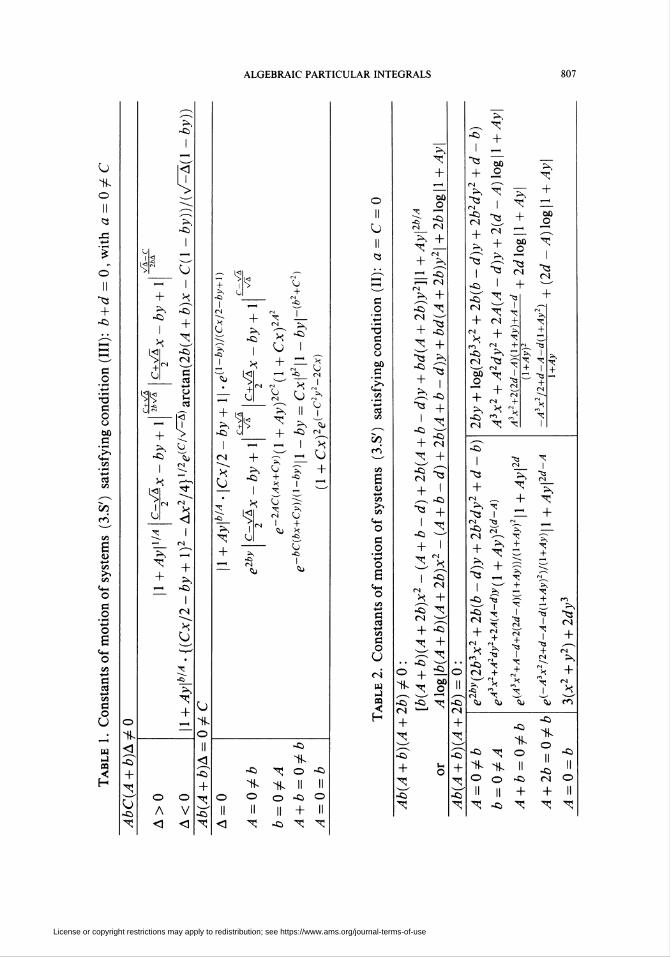
Theorem 3.2. A real quadratic system (3.S) with a center is integrable on R2 or

on the complement of an algebraic curve.

A complete list of constants of motions for quadratic systems with a center

is formed by Tables 1 and 2 (which correspond to conditions (HI) and (II)), the

constant of motion given by the formula (3.4) for the Hamiltonian case and the

rational function (4.24) in §4, constant of motion corresponding to condition

(I) for the case a ¿ 0.

4. Bifurcation diagrams for quadratic systems with a center

(H) is the only one of the four conditions for the center listed in Theorem

3.1, which has a clear geometric meaning: the integral curves of a system (3.S')

satisfying this condition lie on cubic curves, the level curves of the cubic Hamil-

tonian of the system. Is there a geometrical meaning in each one of the other

three conditions for the center? To see this, we draw bifurcation diagrams forconditions (III), (II), and (I) in Theorem 3.1 and then analyze these to see the

geometrical properties which the phase portraits have in common.

Phase portraits of quadratic systems with a center were first drawn by From-

mer [10]. Frommer's paper contains errors (we discussed these in [37]) and from

the 32 phase portraits of the quadratic systems with a center he only drew 15.

Phase portraits of quadratic systems with a center appeared later in a sequence

of papers [20, 22, 23, 25, 44]. We found errors in [25]. In [44] it is stated thatthe list in [20] contains a portrait which cannot be realized and the remaining

ones do not form a complete list. The list in [44] turned out to be complete

but a global dynamic picture does not emerge from this list since these phase

portraits are not assembled in a bifurcation diagram. We obtained bifurcation

diagrams corresponding to the systems with a center and those corresponding

to the three conditions for the center (I), (II), (III) appeared in [32]. These

diagrams lie in the real four-dimensional projective space.

To draw the phase portraits of the plane vector fields, we use the Poincaré

compactification (cf. [29, 13]) of these on the sphere via the central projec-tion. To be precise, the plane Z = 1 in the space coordinates X, Y, Z is

projected on the sphere of radius one centered at the origin. We use the co-

ordinates x = X, y = Y in the plane Z = 1 . The central projection sends

the point (x, y) of this plane on two opposite points on the sphere. A vector

field on the complement of the equator of the sphere is thus obtained and there

exists an analytic vector field defined on the whole sphere (cf. [13]), which gives



by a time rescaling the original polynomial vector field on the corresponding

chart. We denote the coordinates in the associated affine local charts corre-

sponding to points on the sphere belonging to Ux = {(X, Y, Z)\X ^ 0) and

to Uy = {(X, Y, Z)\Y ^ 0) respectively by (u, z) and (v, z). For points

on the sphere belonging to Uz = {(X, Y, Z)\Z ^ 0} the local coordinates

are x, y. The connecting maps between the charts are (x, y) = (X, Y, 1 ) —>

(Y/X,l/X) = (u,z) and (x, y) = (X, Y, I) ^ (X/Y, 1/Y) = (v, z). Ex-cept for the orientation of the integral curves, the vector field behaves similarly

on the north (Z > 0) and south (Z < 0) hemispheres. A compactification

of our vector field is obtained from the restriction of the sphere field on the

northern hemisphere completed by the equator. To view this field, we project

this hemisphere vertically on the (x, y) plane which is the plane Z = 1 and

we draw the phase portraits on the resulting disk where on the circumference

we have the behaviour at infinity.

We consider now the parameter space where the bifurcation diagrams will be

described. The space Q of all systems (3.1) with / and g quadratic polyno-

mials is an open set of a 12-dimensional vector space formed by the coefficients

of / and g . The groups of affine coordinate transformations of the plane and

of positive rescaling of time, act on Q. The orbit space Q of the group action

is five-dimensional and in Q lies the orbit space C of the subspace C of all

quadratic systems with a center. Since the singularities with at least one zero

eigenvalue, of the quadratic vector fields cannot be centers ([4, 43, 17]), we

may assume the systems to be of the form (3.S) or (3.S') and we only need to

consider the group action on such systems (3.S'). The space C is the union of

the orbits under the group action of systems of type (III), (II), (I), and (H) of

Theorem 3.1.Since the group of homotheties of the plane acts on the systems (3.S'), the

parameters a, b, d, A, C are homogeneous coordinates of the system (3.S')

in the projective space P^CR) where the bifurcation diagrams corresponding to

conditions (I), (II), and (III) lie.

The bifurcation diagram corresponding to condition (III). The systems here are

of the form (3.S') with b + d = 0 and they form a hyperplane in T^R). In[10], Frommer observed that the condition a + c = 0 = b + d is preserved under

a rotation of axes. After performing a rotation of axes of an angle 8 , the new

coefficient a' of x2 in the second equation of (3.S) becomes

a! = a cos3 8 + (3b + a) cos2 8 sin 6 + (3c + ß) cos 8 sin2 B + d sin3 8.

Thus, if a / 0, we may always find B such that a' = 0. Hence to draw the

bifurcation diagram of the orbit space associated with the group action for the

case (III) it suffices to consider systems (3.S') with a = 0

(4.1) -r- = -y - bx2 - Cxy - dy2, -+- = x + Axydt dt

with b + d = 0. These systems form a plane parametrized by b , C, A one

of them being nonzero for a nonlinear system. A similarity may be used to

render one of the parameters equal to one. We first consider the case C ^ 0.

These form an affine plane parametrized by (b/C, A/C) or assuming C = 1 ,

by (b, A). The bifurcation diagram in this case is drawn in the affine plane

(b,A).


810 DANA SCHLOMIUK

A particular integral of a system (3.1) (which could be real or complex), is a

curve F(x, y) = 0 such that for all the points on this curve we have

dF dF— (x, y)f(x ,y) + —(x, y)g(x, y) = 0.

For real systems, in the literature sometimes the term invariant curve is used.

To be precise we call invariant set of a real system (3.1) a subset M of R2

such that for every initial condition (t0 = 0 ; Xo, yo), such that (xo, y0) e M,

if (x(t), y(t)), t e (an, ßo), is the unique maximal solution corresponding to

this initial condition, then (x(t), y(t)) belongs to M for all t in its maximal

interval of definition (an, ßo). Clearly a (nonempty) real curve F(x, y) = 0

is invariant for (3.1) if and only if it is a particular integral of the system and

for real systems, the two terms will be used synonymously.

For A ^ 0, the systems (4.1 ) have the invariant straight line 1 + Ay = 0.

For a system (3.S) the origin is either a center or a focus so an invariant straight

line cannot pass through the origin and hence it can be assumed to be of the

form

(4.2) sx + ly+1=0.

Since this line is invariant, for every point on this line we must have sP(x, y) +

lQ(x, y) = 0 where P, Q denote the polynomials on the right-hand side of

(3.S). This is the equation of a conic curve which must have a component in

common with (4.2), i.e., we must have an identity

(4.3) sPix, y) + lQ(x, y) = (sx + ly+ l)(mx + ny)

for some m , n . Straightforward calculations yield:

Proposition 4.1. (i) A system (3.S') has a straight line (4.2) satisfying an identity

(4.3) if and only if b + d = 0 or else a = 0 ^ A . In the first case the system has

at most three such straight lines. If b + d ^0, the straight line is unique and its

equation is I + Ay = 0. (ii) A real quadratic system with a weak focus F and

a real invariant straight line has either a center or a weak focus of order one at

F.

Remark 4.1. Clearly, the presence of two real invariant straight lines of a real

system (3.S'), forces the origin to be a center.

Corollary 4.1. A real quadratic system (3.S') with a center at the origin and

which has an invariant straight line satisfies either the condition (III) or (II).

The basic features of the phase portraits for the case (III) are: the invariant

straight lines, the singular points of the systems in the affine plane (x, y) and

the singular points at infinity. We also have first integrals for case (III) listed in

Table 1.We give the results of the calculations for these basic features of the

phase portraits for case (III). The generic case turns out to be the case when

bACA(A + b) t¿ 0, where A = C2 + Ab(A + b). In this case, for a system (4.1 )satisfying (III), we have two possibilities:

(i) If A < 0 we have only one invariant straight line LA : 1 + Ay = 0. (ii)

If A > 0 then we have three straight lines as particular integrals, i.e., the line

LA : 1 + Ay = 0 and the lines

(4.4) L+, L-: (C ±VÄ)x/2-by+1=0.



These three lines intersect at the singular points.

(4.5) P+,P- = ((C±VÄ)/2Ab,-l/A) and Pb = (0,l/b)

where P+ e LAnL- , T>_ 6 LAC\L+ , and Pb e L+ n L_ . The points at infinityof the invariant lines LA , L+ , L_ are singular points at infinity of the systems:

PooA , P<x>+ , Poo- where

(4.6) PocA = (z = 0,u = 0), andPoo+,Poo- = (z = 0,u = (C±VÄ)/2b).

For the study of the singular points at infinity we use the variables z , u with

the change z = l/x , u = y/x, and z , v with the change z = 1/y , v = x/y

corresponding to the needed two charts. After time rescaling t = zx, the new

equations in (z, u), (z, v) axe respectively:

(4.7)

-j- = z(uz + b + Cu- bu2),dx

-j- = z(l + u2) + u[(A + b) + Cu- bu2],dx

dz , ,, dv ,, . 2\(4.8) ^- = -zv(z + A), ^- = -z(l+v2)-(A + b)v2-Cv + b.

dx dx

For the three singular points (4.6) we have real eigenvalues whose nature is

given by their products

(Xx-X2)ooA = b(A + b),

(Xx-X2)00+=AVÄ(VÄ+C)/2b, (Xx-X2)oc-=AVÄ(VÄ-C)/2b.

We sum up the main features of the phase portraits for case (III) in the

following two propositions.

Proposition 4.2. Consider system (4.1) with b + d = 0 ^ bACA(A + b). Wemay suppose C = 1. We have

If Ab > 0, then A > 0 and the three singular points P+ , P- , Pb are allordinary saddles while the singular points at infinity are all nodes. If Ab < 0 we

distinguish two cases: b(A + b) > 0 and b(A + b) < 0.(i) If b(A + b) > 0 then A > 0, P+ and P- are nodes, Pb is a saddle while

PooA is a node and T^-,., P^- are saddles.

(ii) If b(A + b) < 0 : If A > 0 then P+ , Pb are nodes and P_ is a saddle;PooA , Poo+ are saddles and Poc- is a node. If A < 0 then we have only one

nonzero singular point Pb which is a focus and only one point at infinity Poo/t

which is a saddle.

For the nongeneric case (III) we have

Proposition 4.3. Consider a system (4.1) with b + d = 0 = bAA(A + b), C ^ 0(we may assume C = 1). We have:

If A = 0 then b(A + b) < 0, Ab < 0, P+ = P_ is a saddle-node and Pb isa node. PooA is a saddle, Poo+ = Poo- is a saddle-node.

IfA + b = 0^b then Ab < 0, P_ = Pb is a saddle-node, P+ is a node,PooA - Poo- is a saddle-node, and Poo+ is a saddle.

If b = 0 ¿ A, L+ is Cx + 1 = 0, L,, n L+ = {PA+} where PA+ =(-1/C, -l/A) is a saddle, and Pool+ = (z = 0, v = 0) and PooA = (z =0, u = 0) are saddle-nodes.


812 DANA SCHLOMIUK.

If A = 0 ^ b we have A > 0, Pb is a saddle, Poo+ , P^- are saddle-nodesand z = 0 = u is a node.

If A = 0 = b, the system has only one singular point (0,0), one invariant

line L+ and two points at infinity (as well as their opposites): z = 0 = v which

is a degenerated singular point of trace -C and it is a saddle and z = 0 = u

which is a degenerated singularity of trace 0.

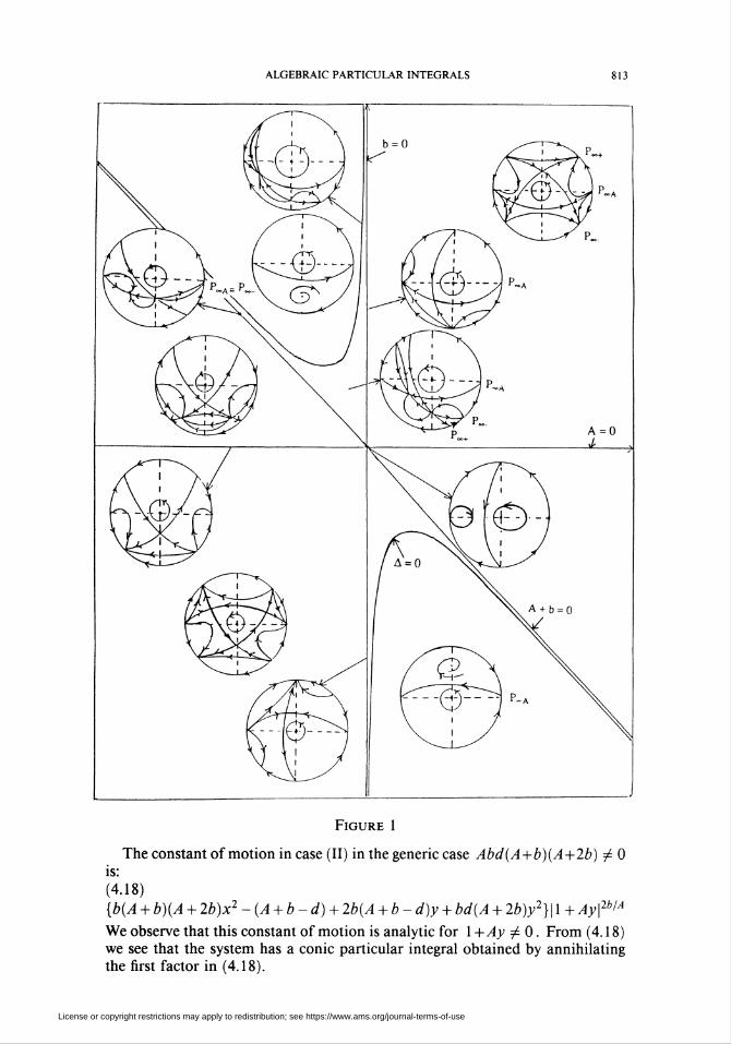
Using all this information, we draw the bifurcation diagram for case (III),

with C t¿ 0. We may assume C = 1 . This bifurcation diagram is drawn in

the plane (b, A) and it appears in Figure 1. The bifurcation lines are: the

hyperbola A = 0, the lines b = 0, A = 0, and A + b = 0. The line at infinityof this affine plane, when completed, is C = 0 = a = b + d and it also belongs

to the bifurcation diagram corresponding to condition (II). We postpone the

drawing of the full bifurcation diagram for (III) on a disk representing T^R)

when opposite points of the circumference are identified, until we complete the

bifurcation diagram for case (II).

The bifurcation diagram corresponding to case (II), i.e., a = 0 = C. Case (II)

is the symmetric case with respect to the y-axis:

Proposition 4.4. A vector field (3.S') is symmetric with respect to the y-axis if

and only if it satisfies a = 0 = C.

The systems satisfying condition (II) are of the form

(4.10) ^ = -y-bx2-dy2, ^ = x + Axy.

We calculate the basic features of the phase portraits in this case. By Propo-

sition 4.1 if A(b + d) ^ 0, such a system has a unique invariant straight line

LA : l+Ay = 0. Assuming Abd(A -d)^0 and b(A - d) > 0 then the systemhas three nonzero singular points:

(4.11) Pd = (0,-l/d), P+,P- = (±y/A-d/A2b, -I/A).

We note that P+ , P_ are located on LA . The eigenvalues of P¿ are

(4.12) Xxd,X2d = ±Vd-A/d

and those of P+ , P- axe

(4.13) Xx± = T2b\/A-d/A2b, X2± = ±A\/A-d/A2b.

As before, to determine the behaviour at infinity we use the variables z, u and

z, v and after time rescaling / = zt we obtain the equations:

(4.14) -j- = z(uz + b + du2), -j-= z(l + u2) + u(A + b + du2),dx dx

(4.15) -¡- = -zu(z + A), -T- = -z(l+v2)-((A + b)v2 + d).dx dx

The singular points come in opposite pairs and in the variables z, u they are

(4.16) P^: z = 0 = u, Px±: z = 0, u = ±<J-(A + b)/d.

The eigenvalues of these points are respectively:

(4.17) XXA = b, X2A=A + b; Xx± = -A, X2± = -2(A + b).



Figure 1

The constant of motion in case (II) in the generic case Abd(A+b)(A+2b) ^ 0is:

(4.18){b(A + b)(A + 2b)x2-(A + b-d) + 2b(A + b-d)y + bd(A + 2b)y2}\l+Ay\2blA

We observe that this constant of motion is analytic for 1 +Ay ^ 0. From (4.18)

we see that the system has a conic particular integral obtained by annihilating

the first factor in (4.18).


814 DANA SCHLOMIUK

We give below the essential features of the phase portraits for this generic

case (II).

Proposition 4.5. Consider a system (4.10) in the generic case

Abd(A + b)(b + d)(A - d)(A + b-d)¿0.

We may assume for simplicity that d > 0. Then we have:

(i) The system has four singular points iff biA - d) > 0. If b > 0 andA - d > 0, then we have two saddles: P+ , P- and two centers. If b < 0 and

A - d < 0, Pd is a saddle and P+ , P_ are nodes when A > 0 while P+ , P_are saddles if A < 0. If biA - d) < 0, we have only one nonzero singular point:

Pd which is a center if A- d > 0, b < 0 and it is saddle if A - d < 0, b > 0.(ii) If A + b < 0 we have three pairs of iopposite) singular points at infinity.

PooA is a node for biA + b) > 0 and a saddle for b(A + b) < 0, Poo+ , P^- arenodes if A(A + b) > 0 and saddles if A(A + b) <0. If A + b > 0 we have onlyone pair of (opposite) singular points at infinity. If b > 0, P^ is a node and it

is a saddle if b < 0.(iii) If A + b < 0, the conic integral of the system is a hyperbola. If A + b > 0,

the conic integral is an invariant ellipse if (A + b - d)(b + d)b > 0 and it is a

conic which has only complex points, if (A + b - d)(b + d)b < 0.

The nongeneric cases satisfying (II), i.e., those with

Abd(A - d)(A + b)(A + 2b) = 0 = a = C

axe treated (analogously with our discussion for condition (III)), using the in-

formation contained in equations (4.11 )—(4.18) and in Table 2.

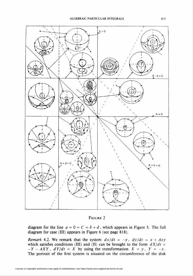
The bifurcation diagram for the case d ^ 0 (we may assume d = 1 ) appears

in Figure 2, except for the orientation of some integral curves, omitted not to

overcrowd the drawing. To follow the change in the systems as parameters vary,

we drew all the phase portraits on this bifurcation diagram and to make this

possible, we varied the scale when drawing our disks. Condition (II) with d / 0

defines an affine plane which is parametrized by (b/d, A/d) ox if we assume

d = 1 , by (b, A). The bifurcation points are located on the lines b = 0,

A - d = 0, A + b = 0, .4 = 0 and on the line b + d = 0. We completethe bifurcation diagram for case (II) by considering what happens in the case

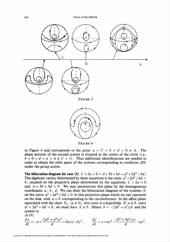
d = 0. The bifurcation diagram for the line a = 0 = c = C = d, A = 1 ,

line parametrized by b, is drawn in Figure 3 (page 816); the bifurcation points

are at b = -A and at b = 0. The point at infinity of this line is the point

C = a = A = d = 0^b. The system corresponding to this point has only one

singular point, the origin and the phase portrait is given in Figure 4. The full

bifurcation diagram for case (II) is drawn on a disk. Inside the disk we place

the bifurcation diagram shown in Figure 2 and on the circle the bifurcation

diagram shown in Figure 3 and completed with its point at infinity for which

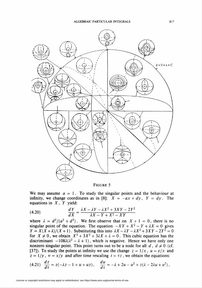
we have the phase portrait given in Figure 4 (page 816). The complete diagramfor condition (II) appears on the disk shown in Figure 5 (page 817) where almost

all the phase portraits are drawn; the missing ones in the central quadrangle and

the orientation of the some of the integral curves could be found in Figure 2.

Finally, we are now in a position to complete on the disk the bifurcation

diagram for case (III). We place inside the disk the bifurcation diagram for the

plane b+d = 0 = a, C/0, drawn in Figure 1 and on the circle the bifurcation


ALGEBRAIC particular INTEGRALS 815

Figure 2

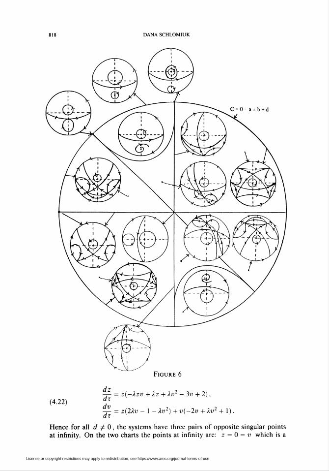
diagram for the line a = 0 = C = b + d, which appears in Figure 5. The full

diagram for case (III) appears in Figure 6 (see page 818).

Remark 4.2. We remark that the system dx/dt = -y, dy/dt = x + Axywhich satisfies conditions (III) and (II) can be brought to the form dX/dt =

-Y - AXY, dY/dt = X by using the transformation X = y, Y = -x.

The portrait of the first system is situated on the circumference of the disk


816 DANA SCHLOMIUK

Figure 3

Figure 4

in Figure 6 and corresponds to the point a = C = b = d = 0^A. The

phase portrait of the second system is situated at the center of the circle (i.e.,

b = 0 = d = a = A^C= 1). Thus additional identifications are needed in

order to obtain the orbit space of the systems corresponding to condition (III)

under the group action.

The bifurcation diagram for case (I): C + 2a = 0 = A + 3b + 5d = a2 + 2d2 + bd.The algebraic variety determined by these equations is the conic a2+2d2 + bd =

0, situated on the projective plane determined by the equations C + 2a = 0

and A + 3b + 5d = 0. We may parametrize this plane by the homogeneous

coordinates a , b , d . We can draw the bifurcation diagram of the systems (I)

on the curve a2 + 2d2 + bd = 0 in this projective plane which we can representon the disk, with a = 0 corresponding to the circumference. In the affine plane

associated with the chart Ua (a ^ 0), this conic is a hyperbola. If a ^ 0, since

a2 + 2d2 + bd = 0, we must have d ^ 0. Hence b = -(2d2 + a2)/d and thesystem is:

(4.19)dx (2d2 + a2)x2 „ , 2 dy 2 (d2 + 3a2)xy-=- = -y+---,—-—+2axy-dy¿, -f- = x+ax1----.—'—^--ay¿.dt d dt d


ALGEBRAIC particular integrals 817

Figure 5

We may assume a = 1. To study the singular points and the behaviour at

infinity, we change coordinates as in [8]: X = -ax + dy, Y = dy. Theequations in X, Y yield:

dY _ XX - XY - XX2 + 3XY - 2Y2

( ' ' ~d~X~ XX-Y + X2-XY

where X = d2/(a2 + d2). We first observe that on X + 1 = 0, there is no

singular point of the equation. The equation -XY + X2 - Y + XX = 0 gives

Y = X(X + X)/(X+l). Substituting this into /Uf-/iy-/Uf2 + 3*Y-2r2 = 0for X ^ 0, we obtain X3 + 3X2 + 3XX + X = 0. This cubic equation has thediscriminant -108a(A2 - X + 1), which is negative. Hence we have only one

nonzero singular point. This point turns out to be a node for all d , d ^ 0 (cf.

[37]). To study the points at infinity we use the change z = 1/x , u = y/x and

z = 1/y , v = x/y and after time rescaling / = tz , we obtain the equations:

(4.21) -¡-= z(-Xz-l + u + uz), -1-=-X + 2u-u2 + z(X-2Xu + u2),dx dx


818 DANA SCHLOMIUK

Figure 6

(4.22)

-r- = z(-Xzv + Xz + Xv2 -3v + 2),dx(11)— = z(2Xv- 1 -Xv2) + v(-2v+Xv2 + 1)

Hence for all d ^ 0, the systems have three pairs of opposite singular points

at infinity. On the two charts the points at infinity are: z = 0 = v which is a


ALGEBRAIC PARTICULAR INTEGRALS

Figure 7

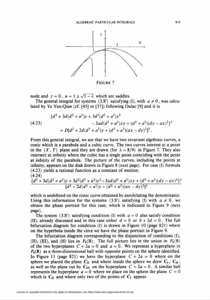
node and z = 0, u = 1 ± y/l - X which are saddles.The general integral for systems (3.S') satisfying (I), with a ^ 0, was calcu-

lated by Ye Yan-Qian (cf. [45] or [37]) following Dulac [9] and it is

{d2 + 3d(d2 + a2)y + 3d2(d2 + a2)y2

(4.23) - 3ad(d2 + a2)xy + (d2 + a2)(dy - ax)3}2

= D[d2 + 2d(d2 + a2)y + (d2 + a2)(ax - dy)2]3.

From this general integral, we see that we have two invariant algebraic curves, a

conic which is a parabola and a cubic curve. The two curves interest at a point

in the (X, Y) plane and they are drawn (for X = 8/9) in Figure 7. They also

intersect at infinity where the cubic has a single point coinciding with the point

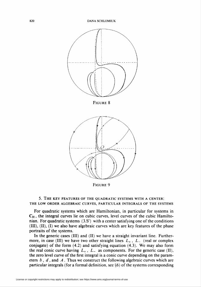
at infinity of the parabola. The picture of the curves, including the points at

infinity, appears on the disk drawn in Figure 8 (next page). For case (I) formula

(4.23) yields a rational function as a constant of motion:

(4.24){d2 + 3d(d2 + a2)y + 3d2(d2 + a2)y2-3ad(d2 + a2)xy + (d2 + a2)(dy - ax)3}2

[d2 + 2d(d2 + a2)y + (d2 + a2)(ax - dy)2]3

which is undefined on the conic curve obtained by annihilating the denominator.

Using this information for the systems (3.S') satisfying (I) with a / 0, we

obtain the phase portrait for this case, which is indicated in Figure 9 (next

page).

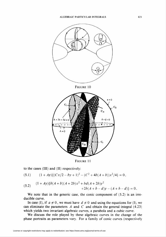
The system (3.S') satisfying condition (I) with a = 0 also satisfy condition

(II), already discussed and in this case either d = 0 or b + 2d = 0. The fullbifurcation diagram for condition (I) is drawn in Figure 10 (page 821) where

on the hyperbola inside the circe we have the phase portrait in Figure 9.

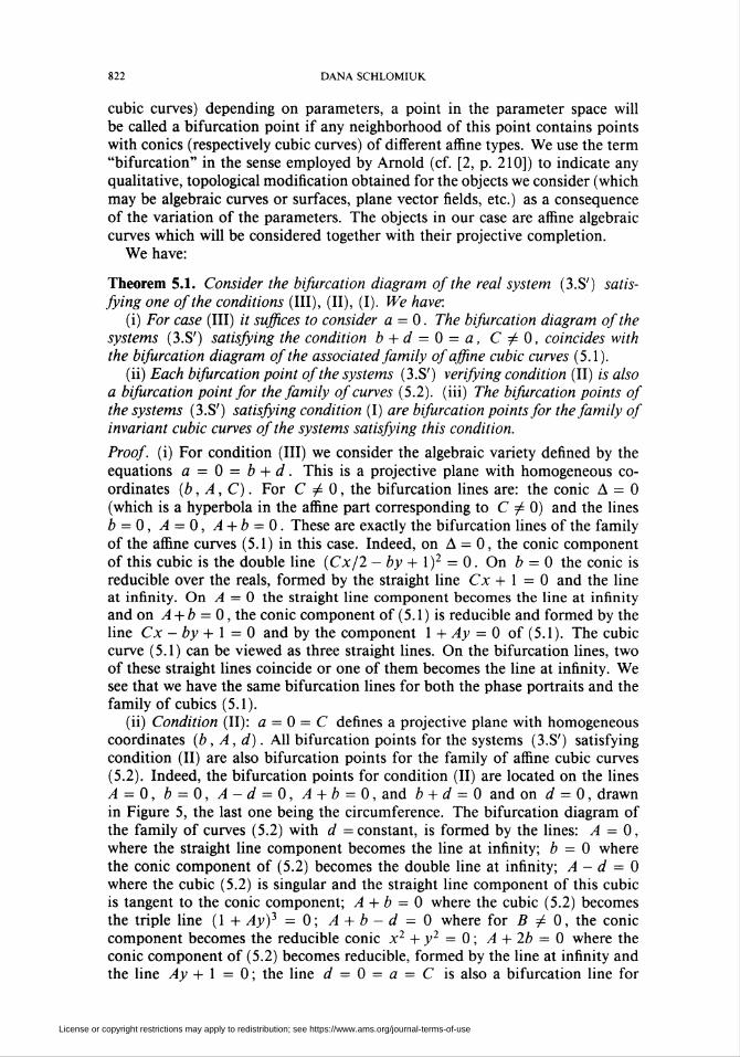
The bifurcation diagram corresponding to the disjunction of conditions (I),

(II), (III), and (H) lies in P4(R). The full picture lies in the union in P4(R)of the two hyperplanes C + 2a = 0 and a = 0. We represent a hyperplane in

P4(R) as a three-dimensional ball with opposite points on the sphere identified.

In Figure 11 (page 821) we have the hyperplane C + 2a = 0 where on the

sphere we placed the plane C» and where inside the sphere we drew Q , Ch ,

as well as the plane cut by Cm on the hyperplane C + 2a = 0. A similar ball

represents the hyperplane a = 0 where we place on the sphere the plane C = 0

which is Cu and where only two of the points of Cx appear.


820 DANA SCHLOMIUK

Figure 8

Figure 9

5. The key features of the quadratic systems with a center:

the low order algebraic curves, particular integrals of the systems

For quadratic systems which are Hamiltonian, in particular for systems in

Ch , the integral curves lie on cubic curves, level curves of the cubic Hamilto-

nian. For quadratic systems (3.S') with a center satisfying one of the conditions

(III), (II), (I) we also have algebraic curves which are key features of the phase

portraits of the systems.

In the generic cases (III) and (II) we have a straight invariant line. Further-

more, in case (III) we have two other straight lines L+ , L_ (real or complex

conjugate) of the form (4.2) and satisfying equation (4.3). We may also form

the real conic curve having L+ , L_ as components. For the generic case (II),

the zero level curve of the first integral is a conic curve depending on the param-

eters b , d, and A . Thus we construct the following algebraic curves which are

particular integrals (for a formal definition, see §6) of the systems corresponding



Figure 11

to the cases (III) and (II) respectively:

(5.1) (1 + Ay){(Cx/2 -by+ I)2 - (C2 + 4b(A + b))x2/4} = 0,

(1+ Ay){b(A + b)(A + 2b)x2 + bd(A + 2b)y2

+2b(A + b-d)y-(A + b-d)} = 0,

We note that in the generic case, the conic component of (5.2) is an irre-

ducible curve.

In case (I), if a / 0, we must have d ^ 0 and using the equations for (I), we

can eliminate the parameters A and C and obtain the general integral (4.23)

which yields two invariant algebraic curves, a parabola and a cubic curve.

We discuss the role played by these algebraic curves in the change of the

phase portraits as parameters vary. For a family of conic curves (respectively


822 DANA SCHLOMIUK

cubic curves) depending on parameters, a point in the parameter space will

be called a bifurcation point if any neighborhood of this point contains points

with conies (respectively cubic curves) of different affine types. We use the term

"bifurcation" in the sense employed by Arnold (cf. [2, p. 210]) to indicate any

qualitative, topological modification obtained for the objects we consider (which

may be algebraic curves or surfaces, plane vector fields, etc.) as a consequence

of the variation of the parameters. The objects in our case are affine algebraic

curves which will be considered together with their projective completion.

We have:

Theorem 5.1. Consider the bifurcation diagram of the real system (3.S') satis-

fying one of the conditions (III), (II), (I). We have:(i) For case (III) it suffices to consider a = 0. The bifurcation diagram of the

systems (3.S') satisfying the condition b + d = 0 = a, C ^ 0, coincides with

the bifurcation diagram of the associated family of affine cubic curves (5.1).

(ii) Each bifurcation point of the systems (3.S') verifying condition (II) is also

a bifurcation point for the family of curves (5.2). (iii) The bifurcation points of

the systems (3.S') satisfying condition (I) are bifurcation points for the family of

invariant cubic curves of the systems satisfying this condition.

Proof, (i) For condition (III) we consider the algebraic variety defined by the

equations a = 0 = b + d. This is a projective plane with homogeneous co-

ordinates (b, A, C). For C t¿ 0, the bifurcation lines are: the conic A = 0

(which is a hyperbola in the affine part corresponding to C ^ 0) and the lines

b = 0, A = 0, A + b = 0. These are exactly the bifurcation lines of the family

of the affine curves (5.1) in this case. Indeed, on A = 0, the conic component

of this cubic is the double line (Cx/2 - by + I)2 = 0. On b = 0 the conic isreducible over the reals, formed by the straight line Cx +1=0 and the lineat infinity. On A = 0 the straight line component becomes the line at infinity

and on A + b = 0, the conic component of (5.1 ) is reducible and formed by the

line Cx - by + 1 = 0 and by the component I + Ay = 0 of (5.1). The cubiccurve (5.1) can be viewed as three straight lines. On the bifurcation lines, two

of these straight lines coincide or one of them becomes the line at infinity. We

see that we have the same bifurcation lines for both the phase portraits and the

family of cubics (5.1).(ii) Condition (II): a = 0 = C defines a projective plane with homogeneous

coordinates (b, A, d). All bifurcation points for the systems (3.S') satisfying

condition (II) are also bifurcation points for the family of affine cubic curves

(5.2). Indeed, the bifurcation points for condition (II) are located on the lines

A = 0, b = 0, A- d = 0, A + b = 0, and b + d = 0 and on d = 0, drawnin Figure 5, the last one being the circumference. The bifurcation diagram of

the family of curves (5.2) with d = constant, is formed by the lines: A = 0,

where the straight line component becomes the line at infinity; b = 0 where

the conic component of (5.2) becomes the double line at infinity; A - d = 0where the cubic (5.2) is singular and the straight line component of this cubic

is tangent to the conic component; A + b = 0 where the cubic (5.2) becomes

the triple line (1 + Ay)3 = 0; A + b - d = 0 where for fi/0, the coniccomponent becomes the reducible conic x2 + y2 = 0 ; A + 2b = 0 where the

conic component of (5.2) becomes reducible, formed by the line at infinity and

the line Ay + 1 = 0 ; the line d = 0 = a = C is also a bifurcation line for


ALGEBRAIC PARTICULAR INTEGRALS

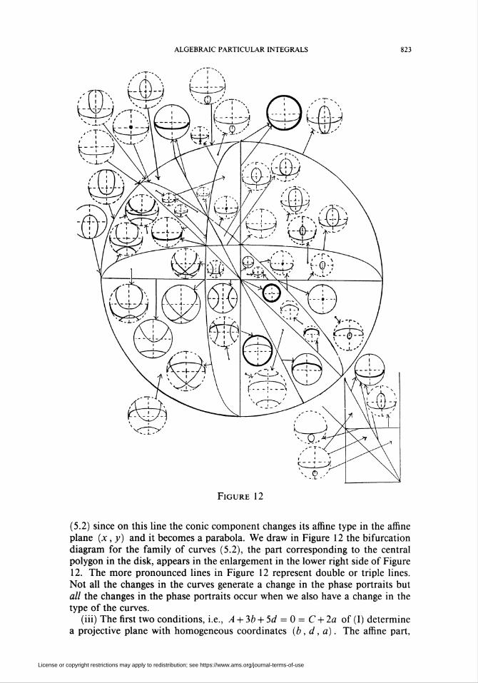
Figure 12

(5.2) since on this line the conic component changes its affine type in the affine

plane (x, y) and it becomes a parabola. We draw in Figure 12 the bifurcation

diagram for the family of curves (5.2), the part corresponding to the central

polygon in the disk, appears in the enlargement in the lower right side of Figure

12. The more pronounced lines in Figure 12 represent double or triple lines.

Not all the changes in the curves generate a change in the phase portraits but

all the changes in the phase portraits occur when we also have a change in the

type of the curves.

(iii) The first two conditions, i.e., A + 3b + 5d = 0 = C + 2a of (I) determinea projective plane with homogeneous coordinates (b, d, a). The affine part,


824 DANA SCHLOMIUK

for a ^ 0, of the curve a2 + 2d2 + bd = 0, determined by the third condition

in (I) is a hyperbola. This conic cuts the line a = 0 of this plane at the points

(b, 0,0) and (-2d, d, 0), both of them situated on the bifurcation diagram

for case (II). If a ^ 0, then all the phase portraits are of one type, namely

the one indicated in Figure 9. So the bifurcation diagram for condition (I) are

exactly the two points mentioned above and these are also points of bifurcation

for the invariant cubic curves in this case. Indeed, for a ^ 0 the invariant

cubics are irreducible, while for a = 0 they are reducible curves. D

Remark 5.1. The restriction C ^ 0 imposed in point (i) of the preceding theo-

rem is necessary there because in (i) we consider only case (III). The points of

the line C = 0 = b + d = a, located on the circumference of the disk in Figure

6, are all bifurcation points for the systems (3.S') with a center at the origin

but only a segment of this line is made of bifurcation points for systems of type

(HI) while the remaining segment of this line is made of bifurcation points for

systems of type (II), segment which also appears in Figure 2. All points of this

line are also bifurcation points for the family of cubic particular integrals of the

systems (3.S') with a center at the origin.

Remark 5.2. We point out a striking particular instance of change in phase

portraits produced by a bifurcation of invariant algebraic curves: Consider the

bifurcation line b + d = 0 in Figure 2, in the part A < 0. On both the leftand right side of this line and on the line, the phase portraits have exactly three

singular points in the plane (x, y) which are all saddles and three pairs of

opposite singular points at infinity, all nodes. The phase portraits on the left

of the bifurcation line have a singular cycle with two singular points, on the

bifurcation line they have a singular cycle with three singular points and on

the right a singular cycle with just one singular point, i.e., a homoclinic loop.

This complete difference in phase portraits is forced by the bifurcation of the

invariant hyperbola on both sides of the bifurcation line b + d = 0, which

becomes a pair of intersecting straight lines on b + d = 0.

6. Algebraic particular integrals of polynomial vector fields

The importance of the algebraic particular solutions of polynomial differen-

tial equations was first observed by Darboux in [7].

In this paragraph we consider algebraic particular integrals of general poly-

nomial vector fields, but to be specific we illustrate our discussion by obtaining

some results for the quadratic systems with a weak focus.

By a particular integral of a real system

(6.1) d^t=P(x,y), ^ = Q(x,y)

it is usually meant a (nonempty) real curve F(x, y) = 0 such that for all the

points on this curve we have

(6.2) !£(* • y)p(* ' y) + zr^x > y^x >y) = °-

If the curve is algebraic then F is of the form

(6.3) F(x,y) = Fn(x,y) + F„-.x(x,y) + --- + Fx(x,y) + F0(x, y)


ALGEBRAIC PARTICULAR INTEGRALS X25

where F¡(x, y) is a homogeneous polynomial with real coefficients of degree

i.

If for some K (x, y) e R[x, y] we have

(6.CT) ^LP+yLQ = F{x, y)K{x ; y) .

then clearly F(x, y) = 0 is a particular integral of (6.1).

If there exists a curve F(x, y) = 0 satisfying (6.CT) for some real poly-

nomial K, then (6.CT) is a computational tool for the determination of the

coefficients of F ; we shall use it to calculate the conies and cubics, particular

integrals of (3.S'). Let us denote by P,, Q, the homogeneous polynomials of

degree i in P, respectively Q of (6.1). To be specific we consider systems

(3.S') where we have P = Px + P2, Q = QX+Q2 and the identity (6.CT) is ofthe following form:

(6.CT2) ^Lp+yLQ = F{x,y){uX + Vy + w).

Our analysis of the quadratic systems with a center gives us:

Proposition 6.1. Assume that a system (3.S') has a center at the origin. Then,

generically, this system has either a straight line and a conic curve (not passing

through the origin) satisfying an identity (6.CT2) or it has no invariant straight

line but it has a conic and a cubic curve, both irreducible over C as particular

integrals or it is a Hamiltonian system. For each one of these particular integrals

F(x, y) = 0 an identity (6.CT2) holds.

Remark 6.1. In the case of a real algebraic curve F(x, y) = 0, irreducible over

C, which has an infinity of points in R2 and which is a particular integral of

system (6.1), (6.CT) holds since the curve must have a component in common

with F'(x,y) = 0, where F' = (dF/dx)P + (dF/dy)Q. So, for algebraiccurves which are irreducible and which have an infinity of points in R2, (6.CT)

is equivalent to the real curve being a particular integral for the real system (6.1 ).

Even if we are primarily interested in real systems, the polynomial identity

(6.CT) is useful beyond the calculation of the irreducible real algebraic curves

which have an infinite number of points in R2 and which are particular integrals

of the systems. Indeed, for example the conic component of (5.2) has no real

point, for the parameter values such that 0 < A + b < d, A - d > 0, and

b + d < 0. Nevertheless, as seen in §5, this conic component has its role. So

in the final analysis, real curves with only complex points, as well as those with

a finite number of real points, need to be considered. What matters is that

these curves satisfy an identity (6.CT). So, from now on, we shall use the term

"algebraic particular integral", according to the following definition:

Definition 6.1. By an algebraic particular integral of a polynomial system (6.1),

real or complex, we shall mean an algebraic curve F(x, y) = 0, real or complex,

such that an identity (6.CT) holds for some polynomial K (x, y) with real or

complex coefficients.

For an algebraic curve F(x,y) = 0 with F of degree n, (6.CT2) yields

n + 2 equations, one for each coefficient of a degree / term, with 0 < / <

n + 1 . Identifying the corresponding coefficients of the zero degree terms, we


826 DANA SCHLOMIUK

get FoW = 0 and assuming F0 # 0, we have w = 0. Identifying the coefficients

of the degree 1 terms in (6.CT2) we have u = aoX, v = -aXo . Identifying the

coefficients of the degree i terms in (6.CT2), with 2 < i < n , we have

(6.CT2UtF) ^PX + ^Qx + d-^P2 + ^Q2 = Ft_x(aoXx - axoy)

while identifying the coefficients of degree n + 1 in (6.CT2) we have

(6.CT2.n+UF) d-^P2 + d-^-Q2 = Fn(aoxx - axoy).

The above equation becomes a particular instance of equation (6.CT2;¡,/0 fori = n + 1 if we write

F(x, y) = Fn+X(x,y) + Fn(x,y) + --- + Fx(x,y) + F0,

with F„+X(x, y) = an+x;0x"+1 + • • • + ao,n+\y"+]

with a¡j = 0, i + j = n + 1.

In general, if we look for an algebraic integral F(x, y) = 0 of degree n + 1

after we discussed the algebraic integrals F(x, y) = 0 of degree n, we note

that the equations obtained by identifying the terms of degrees i with i < n

in (6.CT2) are the same for curves of degrees n and n + 1. The last equation

used for curves of degree n is (6.CT2;,,f) with i = n+l and Fn+X(x, y) with

zero coefficients while for a curve of degree n + 1, we have two other equations

(6.CT2;,,f ) obtained by identifying the remaining coefficients of the terms of

the degrees i = n + 2 and i = n+l in (6.CT2) where we write F = £^=o+2 fi

with Fn+2(x, y) = Dl+y=„+2 aijx'yj with au = 0.

In particular if we want to compute the conies and cubics, we first identify

the coefficients of the degree 2 terms and this will give us some of the coefficientsof F2 . These coefficients are also used when we compute the cubic integrals.

We illustrate the computation of invariant algebraic curves with some results

concerning the existence of invariant conic curves for a system (3.S'). Straight-

forward calculations (cf. [34]) yield

Proposition 6.2. Assume that the real system (3.S') has a conic curve F(x, y) =

0, with real coefficients, passing through the origin and such that F divides

(dF/dx)P + (dF/dy)Q, where P and Q are the polynomials on the righthand side of (3.S'). Then the conic is x2 + y2 = 0 and the coefficients of the

system satisfy the conditions: C = 2a and A + b - d = 0.

From the identity (6.CT2), straightforward calculations also yield the fol-

lowing:

Proposition 6.3. If a real quadratic system (3.S') satisfying condition (III) has a

conic curve F(x, y) = 0, not passing through the origin as an algebraic particular

integral, then this conic is either reducible over C or else the system can be

brought via a coordinate change, to one of the same form (3.S'), satisfying b +

d = 0 and with a = 0=C = A + 2b, in which case the conic is

(6.4) a20(x2+y2)-2¿>y+l =0.

Theorem 6.1. Assume that a system (3.S') with b + d / 0, has a conic curve

F(x, y) = 0, not passing through the origin as an algebraic particular integral.

If this conic is irreducible, then we have the following possible situations:



(i) If a t¿ 0, then necessarily d ^ 0, the coefficients of the system must satisfy

the following two equations:

(6.5) 2d2 + bd-aC-a2 = 0,

(6.6) d(C + a)(A - d) + 2a(C + a)2 - ad(2d + b) = 0,

and the conic is a parabola whose equation is

(6.7) (d2 -aC- a2){(ax - dy)2 + 2dy} + d2 = 0.

(ii) If a = 0, then necessarily C = 0 and hence (II) holds. We have: IfA + b - d ,¿ 0, then b(A + b)(A + 2b) ^¿ 0, the conic is unique and its equation

in this case is

(6.8) b(A + b)(A + 2b)x2 + bd(A + 2b)y2 + 2by(A + b-d)-(A + b-d) = 0.

IfA + b-d = 0 then bd = 0 and the conic is anyone of the one-parameter

family of curves

(6.9) a20x2 + (b2 + a20)y2 -2by+l=0.

Proof. We may assume the conic to be F(x, y) = 0 where

(6.10) F(x,y) = a20x2 + 2axxxy + a02y2 + axox + aoxy + 1

with (a2o, axx, ao2) ^ 0. (6.CT2) yields w = 0 and identifying the coefficients

of the terms of order one in (6.CT2) we have

(6.11) m = öoi and v = -aXo-

Identifying the coefficients of x2 and y2 in (6.CT2) we obtain the equations:

(6.12) a.aoX+2axx - baXo-axoaoX =0 (forx2),

(6.13) -a.aox-2axx - daXo + axoaox =0 (fory2).

From these we obtain the equation

(6.14) axo(b + d) = 0

and, since b + d / 0, we get aXo = 0. Replacing this in (6.12) we obtain the

equation:

(6.15) axx = -a.aoX/2.

Identifying the coefficients of xy in (6.CT2) we obtain

(6.16) 2^02-2a2o + tfoi-4 = «oi •

From (6.16) we obtain

(6.17) a20 = (a0i^ + 2flo2-«oi)/2-

It remains to identify the coefficients of the terms of degree 3 in (6.CT2), i.e.

(6.18) ^ + ^02-Í2a0lx = 0.

In (6.18) we replace the coefficients given by the formulas (6.15) and (6.17)

and identifying the coefficients of the degree 3 terms in (6.18) we obtain the

equations:

(6.19) a(aoXd-2ao2) = 0 (fory3),


828 DANA SCHLOMIUK

-a0XAb - 2a02b + alxb - a\xA/2 - a0iflo2 + a\x/2 - a2a0x =0,

(for x3),(6.20)

(6.21)

(6.22)

-a0XAd - 2a02^ + «oi^ + aaoxC + 2a02A - aoXa02 + a2aox = 0

(for xy2),

-iZoi^C - 2flo2C + a2xC + aaoXb - aao\A + 2aao2 + aalx = 0

(for x2y).

Case a = 0. In this case C = 0. Indeed, if C/0, from (6.22) we musthave

(6.23) ali -2a02-a0xA = 0.

From this we get

(6.24) a02 = (all -a0XA)/2.

We are left with two equations: (6.20) and (6.21) where we replace «02 from

(6.24) and a by zero. (6.20) becomes 0 = 0 and after factoring, (6.21) becomes

(6.25) aox(aox - A)(2A - aox) = 0.

If aoi = 0 then a,v = 0. The case ani = A yields a,j = 0 for i + j = 2. In

the case #oi = 2A the conic is the double line (1 +^4y)2 = 0. So C = 0. Sincea = 0, by (6.15) we have axx = 0 and identifying with zero the coefficients of

x3 in (6.18) we have

(6.26) a20(aoi+2¿>) = 0.

If a2o = 0, the conic is (Ay + l)2 = 0, so from (6.26) have <zoi = -2b andequation (6.16) becomes

(6.27) -fl20 + a02 = b(A + 2b)

while equation (6.21) after simplification by 2 becomes

(6.28) (A + b-d)a02 + bd(A + 2b) = 0.

If A + b - d / 0, the linear system {(6.26), (6.27)} yields

taw „ -bd(A + 2b) -b(A + b)(A + 2b)(6"29) a°2 = A + b-d ' a20 =-T+b—d-•

The conic is

-KA + V,)(A + by* _ M(A h. 2„y _v ' A+b-d A+b-d

and multiplying by A + b-d we obtain (6.8). We observe that this is a true

conic if and only if b(A + 2b) ¿ 0. If A + b = 0, then (6.30) is a doubleline. So A + b ¿0. lfA + b-d = 0 then (6.28) yields bd(A + 2b) = 0.But A + 2b = d + b^0. Hence we must have bd = 0. If b = 0 then«oí = 0 = A - d and from (6.16) we have a20 = aoi ■ In this case the conic is

(6.31) ¿z20(x2 + y2) + l =0.



If d = 0, then A + b = 0 and (6.27) yields <zo2 = b2 + a2o. In this case wehave the one-parameter family of conies (6.9). We note that (6.31) is (6.9) with

b = 0.Case a ^¿ 0. From (6.19) we get

(6.32) a02 = a0xd/2.

Replacing the above in (6.21), we obtain on the left hand side an expression

which factors through «oi • We must have <Zoi ¥" 0 since otherwise all a,j axe

zero. So simplifying by aoi and eliminating the denominators we obtain

(6.33) 2d2 - aoxd - 2a(C + a) = 0.

Using (6.32) and the above equation, we obtain

(6.34) a02 = d2-a(C + a).

We show that we must have d / 0. Indeed, if we suppose d = 0, then by

(6.32) we must have ao2 = 0 and from (6.33) we obtain C + a = 0. Equation

(6.22) yields ab = 0, hence b = 0, contradicting our hypothesis that b+d 7¿ 0.So d # 0 and (6.33) yields

(6.35) «oi =2(d2-a(C + a))/d.

Replacing (6.32) in (6.22), after simplifying by aoX and replacing in the result-

ing equation «oi fr°m (6.35), we obtain

(6.36) Cd2 + 3ad2 - ACd + abd - aAd - 2aC2 - 4a2C -2a3 = 0.

Regrouping the terms above and isolating A we obtain

(6.37) Ad(C + a) = (C + a)d2 + ad(2d + b) - 2a(C + a)2

from which we obtain the equation (6.6) which we had to prove. We distinguish

two possibilities: C + a ^ 0 and C + a = 0. If C + a^0 then we have

(6.38) A = (Cd2 + 3ad2 + abd - 2aC2 - 4a2C - 2ai)/d(C + a).

Replacing (6.32) in (6.20), simplifying by aoi and eliminating the denominator,

we obtain

(6.39) 2bd + ao\d + 2Ab-2aoXb + aoXA-alx + 2a2 = 0.

Replacing (6.35) in the above, eliminating the denominator and simplifying by

2, we get

d4 + bd3 - Ad3 - 3aCd2 - Abd2 - 4a2d2 - 2abCd + aACd(6-40) , . . .

-2a2bd + a2 Ad + 2a2C2 + 4a3C + 2a4 = 0.

Using (6.38) in the above and factoring we obtain

(6.41) -ad2(b + d)(2d2 + bd - aC - a2) = 0,

and since ad2(b + d) ¿ 0, we obtain the equation (6.5) we had to prove. From

(6.5) we get

(6.42) b = -(2d2-aC-a2)/d.

Using the above together with (6.34), (6.35), and (6.38) in (6.17) and (6.15) weobtain the equation (6.7) for the conic.


830 DANA SCHLOMIUK

Assume now that ad ^ 0 = C + a . In this case (6.37) yields 2d + b = 0.

The formula (6.33) yields aoi = 2a1 and (6.34) yields ao2 = d2. Using theseand (6.17) we get a2o = d(A - d). Using formula (6.15) we get an = -ad.From these, (6.20) yields -Ab + bd - Ad + d2 - a2 = 0 and after replacing bby -2a" we get -d2 + Ad - a2 = 0 or a2 = d(A - d). Hence the equation of

the conic is a2x2 - 2adxy + d2y2 + 2dy +1 = 0 or (ax - dy)2 + 2dy +1=0

which is (6.7) with a + C = 0 ^ ad . □

Remark 6.2. We note that if in the above theorem both the system and the

curve are taken with real coefficients, then in view of the Proposition 6.1, the

assumption that the curve pass through the origin may be dropped. In this case,

if a = 0 the origin is a center and the system is integrable.

Corollary 6.1. Assume that a quadratic system has a weak focus of order 1. Sup-

pose that this system has an invariant conic curve, irreducible over C. Then this

conic is a parabola.

We observe that for the case of a degenerate focus, from the Proposition 6.3

and the Theorem 6.1 and the calculations used in the proof of Theorem 6.1, we

obtain the following result which connects the existence of an invariant parabola

with the equation a2 + 2d2 + bd = 0 in condition (I) for the center.

Corollary 6.2. Consider a real system (3.S') which has a degenerate weak focus

at the origin. Assume that the system has a conic curve F(x, y) = 0, F(x, y) e

R[x, y], not passing through the origin, which is an algebraic particular integral

for the system. Then the following conditions hold:

(i) The coefficients of the system must satisfy the equation

a(b + d)(2d2 + a2 + bd) = 0.

(i) The origin is a center and the system is integrable.

Furthermore, if the conic is a parabola, then b + d / 0 and if a ^ 0, we also

have d ^ 0 and

(6.43) A + 3b + 5d = 0 = 2d2 + a2 + bd.

Corollary 6.3. A real quadratic system with a weak focus of order 2 or 3 has no

real algebraic integral which is an irreducible conic curve.

Corollary 6.4. A real quadratic system with a weak focus F and with an irre-

ducible conic curve as an algebraic integral has either a center or a weak focus

of order 1 at F.

The following theorem connects the condition A + 3b + 5d = 0 in (I) with

the existence of a particular cubic integral.

Theorem 6.2. Assume that a system (3.S') with real coefficients has a degenerate

weak focus at the origin. Let us suppose that this system has a cubic curve

F(x, y) = 0 with real coefficients, not passing through the origin, which is an

algebraic particular integral of the system. Then:

(i) The coefficients of the system necessarily satisfy the equation

(6.44) a(b + d)(A - 2b)(A + 3b + 5d) = 0

and if a(b + d)(A - 2b) / 0, then the system satisfies condition (I).



(ii) The origin is a center.

The proof of this theorem is analogous to the proof of Theorem 6.1 (cf.

[36]).

7. A GENERIC CHARACTERIZATION OF QUADRATIC SYSTEMS WITH A CENTER

In this section we determine the geometric content of the conditions for the

center denoted by (III), (II), (I). These conditions correspond respectively to the

three geometric properties denoted by Pm , Pn , Pi in § 1. We show two things:(1) that if a system satisfies the property P, then, via a coordinate change we

can bring the system to the form (3.S') and such that its coefficients satisfy the

condition i, i = III, II, I ; and (2) that the property P, is generic in the set

C, with respect to the usual topology. Each property P, says that the system

possesses two low degree algebraic particular integrals of specific types. In §6 we

obtained the conditions on the coefficients of a quadratic system with a weak

focus, in case the system possesses one algebraic integral of low degree. Now

we consider the case of two algebraic particular integrals and the conditions we

obtain are those for the center.

Let us first assume that part (1) has been proved and let us show part (2). We

consider first the cases / = III, II. In these cases, with the possible exception

of bifurcation points, the system has an invariant straight line L and a conic

particular integral which is not L with multiplicity 2, both not passing through

the origin. Indeed as seen in §4, for the case (III), we may assume a = 0 and

in this case the conic integral (reducible over C) is

(7.1) (Cx/2-¿>y+l)2-Ax2/4 = 0

and in case (II) with Ab(A + b)(A + 2b) / 0, the conic integral is (6.8). Weturn now to condition (I) for the center. We see that if a system (3.S') satisfies

(I) and a ^ 0, then d ^ 0 and the system has the following parabola as a

particular integral

(7.2) d2 + 2d(d2 + a2)y + (d2 + a2)(ax - dy)2 = 0.

Observing the first integral for (I), we see that the following cubic is a particular

integral

(7.3)d2 + 3d(d2 + a2)y + 3d2(d2 + a2)y2 - 3ad(d2 + a2)xy - (d2 + a2)(ax - dy)3 = 0.

We note that this cubic has no singular point in the affine plane and that it has

a singular point at infinity which coincides with the one of the parabola. If this

cubic were reducible, then this point would belong to the components. Since

the curve has no terms in x or in x2, this implies that the curve is irreducible.

Thus a system satisfying (I) with a ^ 0, also satisfies Pi and hence Pi is a

generic property in Q .

It remains to prove the part denoted by ( 1 ) above. We first consider condi-

tions (III) and (II). It follows from the Proposition 4.1, that if a system (3.S')

has two distinct straight lines (possibly with complex coefficients) as integrals,

then the system satisfies (III). We also have the following:

Theorem 7.1. Assume that a system (3.S') with real coefficients possesses an

invariant straight line L and a conic integral F(x, y) = 0, F(x, y) e R[x, y],


832 DANA SCHLOMIUK

which is not the line L with multiplicity 2. Then the system satisfies one of the

two conditions (III): b + d = 0 or (II): a = 0 = C. If the conic integral is

irreducible then in some coordinate axes, the system satisfies (II): a = 0 = C.

Proof. By Proposition 4.1, b + d = 0,oxa = 0^A; assume that b + d ^ 0,then a = 0 ^ A , the system is of the form

(7.4) -^- = -y - bx2 - Cxy - dy2, -j- = x + Axy

and 1 + Ay = 0 is the invariant straight line. If the conic passes through the

origin, then in view of Proposition 6.2 we must have C = 2a and since a = 0,

C = 0. If the conic does not pass through the origin we may assume it to be

F(x, y) = 0 with F given by (6.10). The calculations in the initial part of the

proof of Theorem 6.1, using (6.CT2), apply here and we have (6.12), (6.13)and hence (6.14) from which aXo = 0. From (6.12) we get axx = 0. Identifying

the coefficients of x2y in (6.CT2;„+i,f) with n = 2 we obtain a2oC = 0. If

we assume a2o = 0, then since axx = 0 we must have ao2 ̂ 0. Identifying the

coefficients of xy2 in (6.CT2;„+i,f) with n = 2, we obtain the equation

(7.5) aQ2(2A - aox) = 0

hence aoi = 2A. Identifying the xy coefficients in (6.CT2;„+i,f) with n = 2

and using the other coefficients we obtained so far yields us ao2 = A2 and hence

the conic is ( 1 + Ay)2 = 0, a case ruled out by our hypothesis. So necessarily

we have a2o ^ 0 and C = 0. The last part of the theorem is obtained using

Proposition 6.3. D

We now turn to condition (I).

Theorem 7.2. Assume that a system (3.S') with real coefficients has a parabolaand an irreducible cubic curve as algebraic particular integrals. Assume that the

cubic integral has only one point at infinity which coincides with the one of the

parabola and that it does not pass through the origin. Then the origin is a center,

the coefficients of the system satisfy the conditions

(I) C + 2a = A + 3b + 5d = a2 + 2d2 + bd = 0

and the cubic curve has equation (7.3).

Proof. By Propositions 6.1, 6.3, and Theorem 6.1 we must consider two possi-

bilities. First we consider the case a = 0 in which case C = 0 and the origin is

a center. From Theorem 6.1 we see that the only situation when we could have

a parabola is the case when d = 0. In this case the equation for the parabola

is (6.8). The point at infinity of the homogenized equation is x = 0, y = 1,

z = 0. By hypothesis, this is also the point at infinity of the cubic integral,

so the only cubic term of the cubic integral is fix3 with B / 0. Using the

observation in §6 regarding the calculation of the cubic integrals after we have

computed the conic ones, from (6.12), (6.13) with a = 0 and from (6.14) we

obtain that there are no terms in x or in xy in the equation of the cubic. So

the cubic must be of the form:

(7.6) 5x3+ a2ox2 + a02y2+ aoiy + 1 = 0.

Identifying the coefficients of x2y inequation (6.CT2;;,f) for i = 3 we obtain

B = 0 which is a contradiction. So we must have a ^ 0 in which case d / 0



and by Theorem 6.1 the parabola has equation (6.7) and the coefficients of the

system satisfy conditions (6.5) and (6.6). Since a ^ 0, from equation (6.5) we

obtain

(7.7) C = (2d2 + bd-a2)/a.

Introducing this in (6.6), eliminating the denominator a and then factoring we

obtain

(7.8) d(2d + b)(3d2 + 2bd + Ad-a2) = 0.

Since d t¿ 0, we have two possibilities: b = -2d and

(7.9) 3d2 + 2èd + ^ld-a2 = 0.

Suppose first that b = -2d . In this case (7.7) yields C = -a . We may assume

the cubic curve is of the from F = Fi + F2 + Fx + 1 =0 with F¡ homogeneous

of degree /. Since the cubic has only one point at infinity, coinciding with the

one of the parabola (6.7), we must have F-¡(x, y) = B(ax - dy)3 with B ^ 0.

The calculations at the beginning of the proof of Theorem 6.1 apply for our

cubic F and (6.12), (6.13) hold and hence also (6.14). Since the system has aparabola as integral, b + d / 0 and so aio = 0 and hence we also have (6.15).

The coefficient a2o is given by the formula (6.17). Identifying the terms of

degree 3 in (6.CT2), we have (using aoi = w) :

where P,, Q¡ denote the terms of degree i in the right-hand side of equations

(3.S'). Identifying the terms in y3 we obtain

(7.11) -a(2a02-dw + 3fid2) = 0.

Simplifying by a and solving for ao2 we have

(7.12) a02 = d(u-3Bd)/2.

Next, we equate with zero the coefficient of x2y in (7.10). After replacing in the

equation thus obtained the value for «02 given by (7.12), and using C = -a ,

after factoring we obtain

(7.13) a(2du + bu-3a2B) = 0.

If a ^ 0, under the assumption 2d + b = 0, from the above equation we obtain

fi = 0. So we must have 2d + b ^ 0. This together with d / 0 and (6.5),yield C + a / 0 and equation (7.9) holds. From (7.9) we obtain

(7.14) A = (a2-3d2-2bd)/d.

We replace the above value of A in ß2(x, y) and we identify the terms of

degree 4 in (6.CT2). These give us the equation

(7.15) d~Pi + ^-Q2-Fyux = 0.

Identifying the coefficients of xy3 above, dividing by d3 and solving for u,

we obtain

(7.16) u = -3b -3d.


834 DANA SCHLOMIUK

The coefficients of the other terms of degree 4 in (7.15) are respectively

(7.17) -3ad2(u + 3b + 3d) (for x2y2),

(7.18) 3a2d(u + 3b + 3d) (forx3y),

(7.19) -a3(u + 3b + 3d) (for x4).

All these coefficients become zero if and only if (7.16) holds. Replacing the

value of u from (7.16) in (7.12) we obtain

(7.20) a02 = -3d(Bd + d + b)/2.

Replacing the above in the expression of the coefficient of xy2 in (7.10), after

factoring and multiplying by 2/3d we obtain the equation

(7.21) (3d2 + ¿>d + 2a2)fi + (¿> + d)2 = 0.

Consider now the coefficient of x2y in (7.10). After replacing the value of ao2

given by (7.20), factoring and then multiplying by a/3 we obtain the equation

(7.22) (2d4 + bd3 - a4)B + d(2d + b)(b + d)2 = 0.

Consider now the coefficient of x3 in (7.10). After replacing the value of ao2

like before, factoring and multiplying by -2d¡3 and then regrouping the terms

we obtain the equation

(7.23) d2(3d2 + bd + 2a2)B + (b + d)2(3d2 + bd + a2) = 0.

We need to have a joint solution for equations (7.21), (7.22), and (7.23). We

isolate (b + d)2 from equation (7.21) and replace it in (7.22) and (7.23); after

factoring, we obtain respectively

(7.24) (a2 + 2d2 + ¿>d)2 = 0,

(7.25) -(3d2 + bd + 2a2)(2d2 + bd + a2)B = 0.

From (7.24) we have

(7.26) a2 + 2d2 + bd = 0.

Isolating a2 from (7.26) and replacing this in (7.14) and in (7.7) respectively,

we obtain

(7.27) A + 3b + 5d = 0,

(7.28) C + 2a = 0.

(7.26), (7.27), and (7.28) are conditions (I) and hence by Theorem 3.1 we have

a center at the origin. Let us now calculate the coefficients of the cubic. Using

(7.26) in (7.21) we obtain the following expression for B :

(7.29) B = -(b + d)2/(a2 + d2).

We calculate the remaining coefficients of the cubic. First we solve (7.26) for b

and obtain

(7.30) b = -(2d2 + a2)/d.



Replacing the above in (7.29) and in (7.16) we obtain respectively

(7.31) B = -(d2 + a2)/d2,

(7.32) w = 3(d2 + a2)/d.

We replace the above in (6.15) and we obtain

(7.33) axx = -3a(d2 + a2)/2d.

We replace (7.30) and (7.31) in (7.20) and we obtain

(7.34) a02 = 3(d2 + a2).

Replacing the above and (7.32) in (6.16) yields

(7.35) a20 = 3d(b + d)(2d2 + bd + a2)/2(d2 + a2)

which in view of (7.26) yields a2o = 0. Hence the invariant cubic is

(7.36)_ (d2 + a2)(ax - dy)3 _ 3a(d2 + a2)xy + 2 + a2)y2 + 3(d2 + a2)y + { = Q

d2 d d

and eliminating the denominators we obtain (7.3). D

Since the degenerate singularities of quadratic vector fields cannot be centers

(cf. [4, 43, 17]), the results in this paragraph give us the generic geometric char-

acterization of the center in terms of the algebraic integrals of degrees less than

or equal to 3. If we want to use real curves, the generic geometric characteriza-

tion can be stated as follows:

Theorem 7.3. The following property P is generic for the real plane quadratic sys-

tems with a center: The system has a weak focus F and it is either Hamiltonian

or it has a parabola as particular integral and a real irreducible cubic integral,

not passing through F and which has only one point at infinity coinciding with

the one ofi the parabola, or it has a real invariant straight line and an irreducible

real conic integral, or it has as algebraic particular integrals a real straight line

L and a real conic curve, reducible over C, which is not L counted with multi-

plicity 2 and which does not pass through F. Furthermore, if a quadratic system

has the property P then the system has a center at F.

8. Algebraic particular integrals and integrability,

Darboux's theorem

In this paragraph we consider the results obtained in this work in the perspec-

tive of Darboux's work [7] in which he gives the general integral of a differential

equation defined by polynomials, if we know sufficiently many irreducible alge-

braic particular integrals of the equation.

In [7] Darboux considers differential equations over the projective plane of

the form

(8.1) L(y dz - z dy) + M(z dx - x dz) + N(x dy - y dx) = 0

where L, M, N are homogeneous polynomials in the homogeneous coordi-

nates x, y , z .


836 DANA SCHLOMIUK

Darboux considered particular solutions of (8.1) which are algebraic curves

(8.2) f(x,y,z) = 0

with / a homogeneous polynomial, i.e., curves (8.2) such that the form df is

zero at a point on the curve, on the integral curves of the equation, i.e., such

that on (8.2) we have

(8.3) ^dx + ^dy + ^dz = 0dx dy dz

in the direction of the integral curves. Since / is homogeneous, we also have

(8.4) x^+yd/ + z^ = 0.dx dy dz

From the last two equations, we deduce:

dfi/dx dfi/dy df/dzydz-zdy zdx-xdz xdy-ydx

and hence using (8.1) we obtain

(8.6) Ld/ + M¥ + Nd/ = °-dx dy dx

Darboux remarks that this equation is not necessarily an identity. In fact equa-

tion (8.6) takes place on the curve (8.2). Darboux says: "It will suffice that the

preceding equation takes place only on the points of the curve i.e. that the first

member be divisible by / and that we have identically:

K denoting a polynomial which would necessarily be of degree m - 1 , one less

than the degree of that of L, M, /V".

Remark 8.1. Darboux's work [7], published in 1878, appeared before Hubert's

nullstellensatz. Darboux replaces there "(8.6) holds on all points of the curve

(8.2)" with (8.7). This of course holds for irreducible curves (8.2), when we

work over the complex numbers. Darboux calls such a particular integral, a

particular algebraic solution of the equation.

We are interested here in polynomial vector fields or in first order equations

on the affine plane, not necessarily homogeneous. When written in homoge-

neous coordinates, a differential equation

(8.8) dy/dx = f(x,y)/fx(x,y)

with /, /i polynomials, is a particular case of (8.1). Indeed, written in ho-

mogeneous coordinates, after replacing x, y by x/z, y/z respectively, this

equation gives

(8.9) 4>(x, y, z)(zdx - xdz) + 4>x(x, y, z)(y dz - zdy) = 0

with 4>, 4>x homogeneous polynomials of the same order. The above equation

is a particular instance of (8.1 ), i.e. the case when N = 0. This equation admits

the particular solution z = 0, i.e., the straight line at infinity.


algebraic particular integrals 837

In the first part1 of Darboux's work [7], he states a theorem saying that if we

have sufficiently many algebraic particular integrals of equation (8.1) then we

have a first integral of the equation.

We consider here a version of Darboux's theorem stated in the first part of

[7, p. 79] which applies to this particular situation.

Theorem 8 (Darboux). Let us consider a vector field

X(x, y) = P(x, y)d/dx + Q(x, y)d/dy

with P, Q polynomials over C with m = max(degP, degQ). Let us suppose

that this vector field admits q algebraic particular integrals fi = 0 with i =

I, ... , q, which are irreducible over C. Let dimc Cm_i [x, y] be the dimension

of the complex vector space Cm_ i [x, y] of polynomials of degrees at most m - 1

in the indeterminates x and y and let us suppose that q > dimc Cm._i[x, y].

Then the vector field has a first integral of the form

(8.10) f\lf*?---f\q.Proof. By hypothesis we have irreducible algebraic integrals f(x, y) = 0 of X,

i.e., fi's axe polynomials such that dfi(X) = Kjfi with K e Cm_i[x, y]. Byhypothesis we have q such integrals with q > dime m-i[x,y]= 1 + 2h-\-m =

m(l + m)/2 and hence we have q such polynomials K, of degree m - 1 .

These Kfs must be linearly dependent, i.e., we have complex Ay's such that

\ZUkJKi = °- We obtain (T?j=iWfj/fj)W = 0, i.e., f\l~-f$ is a firstintegral of X.

Remark 8.2. We note that we may have algebraic particular integrals f(x, y) =

0 with / a polynomial with real coefficients, which have no point or only a

finite number of points in the finite plane and these will produce an integral

(8.10) which is a complex multivalued function. For a real constant of motion

we apply absolute values, i.e., \fx \a< |/|22 • • • \fq\ai.

If we have q algebraic integrals with q > m(m + l)/2+ 1 of a vector fieldof degree m , then the exponents Xx, X2, ... , Xq in the constant of motion

/ i'f22 ' " ' f q can be taken to be integers (cf. [41]). Hence in the case given by

Darboux's theorem we have a rational constant of motion. In the case not cov-

ered by Darboux's theorem, i.e., the case when q < m(m + l)/2, we may still

have q linearly dependent Tv,'s and so we may still get a constant of motion.

This is the situation we encountered for systems with a center in the quadratic

case. To apply Darboux's theorem in the particular case of quadratic vector

fields, i.e., m = 2, we need q algebraic irreducible integrals, with q greater

than 3. From four such particular integrals, Darboux's theorem gives us a first

integral of the system which will be rational. Our work shows that for a system

with a weak focus, for each one of the generic cases (III), (II), (I), two such alge-

braic integrals, not passing through the origin, suffice for a constant of motion:

either a straight line and a conic or a conic and a cubic curve. In particular we

point out that we have not used the first integrals of quadratic systems with a

center in the proof of Theorem 7.2 and thus the calculations performed there

give us also a first integral for systems satisfying (I) by using the two algebraic

'This part was not available to the author at the time when this research was done. The author

is thankful to R. Moussu who told her Darboux's theorem and the version we use here.


838 DANA SCHLOMIUK.

integrals we obtained from the hypothesis of the theorem. Analogously, we have

first integrals via algebraic particular integrals for the generic cases of type (II)

and (III) and clearly all these first integrals are elementary.

To compute the algebraic particular integrals F(x, y) = 0 of degree n for

a polynomial vector field dx/dt = P(x, y), dy/dt = Q(x, y) of degree m ,

one uses the polynomial identity (6.CT) of degree n + m - 1 and without

constant terms. This leads to (n + m - l)(n + m)/2 - 1 equations involving

the coefficients aks, bks, fks, gks of the terms in xkys in P, Q, F, and K

respectively. We obtain (n + m — l)(n + m)/2 - 1 equations in the unknowns

fks, Sks and the parameters aks, b^ of the system. To compute the general

integrals we need enough algebraic particular integrals F}■ = 0, i.e., such that the

corresponding Kfs are linearly dependent. By eliminating the unknown Fksj ,

gksj , one finds the compatibility conditions in terms of the parameters a^ ,

bks ■ When these hold, solving the polynomial equations in the unknowns fysj ,

gksj in terms of the parameters gives us the particular algebraic integrals. The

coefficients g^j of the polynomials Kj axe needed in order to obtain the

coefficients of the linear dependence relation required for the calculation of the

first integral.The calculations of algebraic particular integrals of polynomial systems could

be tedious and lengthy even when using computers. Such calculations could be

programmed in MACSYMA or REDUCE for example. These are large, self-

contained systems which do not incorporate mathematical objects like rings,

ideals, and differential forms. Two programs especially designed for commu-

tative algebra are: MACAULEY [42] and COCOA [11]. While these programsare efficient for commutative algebra purposes, they have drawbacks for the

kind of calculations we need here. For example one cannot factor polynomials

in MACAULEY or in COCOA. This is a significant drawback here since weobtained the conditions for the center by factoring polynomials. Once the poly-

nomials are factored, one can check the factorization by hand and hence obtain

a real proof. Usually, it is not possible to obtain the factorization by hand,

the calculations being too massive. In view of these observations, more work

is needed in order to provide us with a program which could efficiently handle

the problem of finding compatibility conditions in terms of parameters and of

solving polynomial equations analogous to those encountered in this work. At

this stage it seems that the best canditate for accommodating such a program is

MAPLE.

Concluding comment and open problems

As we have seen in this work, there is an algebraic geometric structure asso-

ciated to the notion of center, in the case of quadratic differential systems. It is

natural to ask whether there is a corresponding structure in the case of the cubic

systems. Work on the special case of cubic symmetric systems with a center,done by the author together with Ch. Rousseau, shows that the algebraic inte-

grals play a role in these cases, which in part is analogous to what happens in the

quadratic situation. At the conference on bifurcations of planar vector fields

held at Luminy in September 1989, where the author reported on this work,

N. Lloyd reported connections between algebraic particular integrals and the

problem of the center obtained with C. Christopher in two other special cases


algebraic particular integrals 839

of cubic systems but no geometric generic characterization in terms of algebraic

particular integrals was known by them at that time. It is natural to consider

the problem: Determine the role of the algebraic integrals in the theory of the

center for general cubic systems. What are the generic geometric properties of

the cubic systems with a center?

Acknowledgment

The author is very grateful to J. Guckenheimer for raising her interest in

the problem of the center and for asking the key question of the geometrical

meaning of the algebraic conditions for the center. The author is also very

grateful to J. Hubbard and to A. Douady for taking an interest in this work and

to A. Douady, J. Guckenheimer, J. Hubbard, and J. Hurtubise for interesting

and stimulating mathematical discussions. The author also thanks R. Roussarie

who carefully read the manuscript of [32] and who raised some interesting points

concerning that first part of this work. Thanks are also due to R. Moussu who

told the author about Darboux's theorem. Joan C. Artés noticed a wrong ending

of a separatrix in a phase portrait in [32]. Thanks are due to A. Gasull and to J.

Llibre for telling the author about this. The author wishes to thank the referee

for his suggestions concerning improvements in the exposition and the referee,

Ch. Rousseau and J. Carette for final corrections of the manuscript.

This work was done while the author was partly detached to the Centre de

Recherche Mathématique de l'Université de Montréal.

Bibliography

1. D. V. Anosov and V. I. Arnold (Editors), Dynamical systems, vol. I, Encyclopaedia of

Mathematical Sciences, Springer-Verlag, Berlin and New York, 1988, p. 233.

2. V. I. Arnold, Chapitres supplémentaires de la théorie des équations différentielles ordinaires,

"Mir," Moscow, 1980, p. 323. (Translation of the Russian 1978 edition published by

Nauka.)

3. N. N. Bautin, On the number of limit cycles which appear with the variation of the coefficients

from an equilibrium position of focus or center type, Mat. Sb. 30 (72) (1952), 181-196;

English transi, in Math. USSR-Sb. 100 (1954), 397-413.

4. V. Berlinskii, On the behaviour of the integral curves of a differential equation, Izv. Vyssh.

Uchebn. Zaved. Mat. 2 (15) (1960), 3-18. (Russian)

5. F. Browder (Editor), Mathematical developments arrising from Huberts problems, Proc.

Sympos. Pure Math., vol. 28, Amer. Math. Soc, Providence, R.I., 1976, pp. 50-51.

6. Yuanshun Chin (Yuanshun Qin), On surfaces defined by ordinary differential equations,

Lecture Notes in Math., vol. 1151, Springer-Verlag, Berlin and New York, 1985, pp. 115-

131.

7. G. Darboux, Mémoire sur les équations différentielles algébriques du premier ordre et du

premier degré (Mélanges), Bull. Sei. Math. (1878), 60-96, 123-144, 151-200.

8. T. D. Davies and E. M. James, Nonlinear differential equations, Addison-Wesley, Reading,

Mass., 1966, p. 191.

9. H. Dulac, Détermination et integration dune certaine classe d'équations différentielle ayant

pourpoint singulier un centre, Bull. Sei. Math Sér. (2) 32 (1908), no. 1, 230-252.

10. M. Frommer, Über das Auftreten von Wirbeln und Strudeln (geschlossener und spiraliger

Integralkurven) in der Umgebung rationaler Unbeslimmheitsstellen, Math. Ann. 109 (1934),

395-424.

H.A. Giovini and G. Niesi, Cocoa user's manual, Department of Mathematics, University of

Genova, 1989.


840 DANA SCHLOMIUK

12. F. Göbber and K. D. Willamowski, Ljapunov approach to multiple Hopf bifurcation, J. Math.

Anal. Appl. 71 (1979), 333-350.

13. E. A. González Velasco, Generic properties of polynomial vector fields at infinity, Trans.

Amer. Math. Soc. 143 (1969), 201-222.

14. J. Guckenheimer, R. Rand, and D. Schlomiuk, Degenerate homoclinic cycles in perturba-

tions of quadratic hamiltonian systems, Nonlinearity 2 (1989), 405-418.

15. D. Hubert, Mathematische Probleme (lecture), Second Internat. Congress Math. Paris, 1900,

Nachr. Ges. Wiss. Gottingen Math.-Phys. Kl. 1900, pp. 253-297; reprinted in [5, p. 134].

16. Ju. S. Il'yashenko, Perturbations of the polynomial Hamiltonian equations in the real and

complex domains, Sympos. Methods of the Qualitative Theory and the Theory of Bifurca-

tions, Gorky, 1988, pp. 63-67.

17. P. de. Jager, Phase portraits of quadratic systems—higher order singularities and separatrix

cycles, Doctoral Thesis, May 1989, Technische Universiteit Delft.

18. W. Kapteyn, On the midpoints of integral curves of differential equations of the first degree,

Nederl. Akad. Wetensch. Verslag. Afd. Natuurk. Konikl. Nederland. (1911), 1446-1457.(Dutch)

19. _, New investigations on the midpoints of integrals of differential equations of the first

degree, Nederl. Akad. Wetensch. Verslag Afd. Natuurk. 20 (1912), 1354-1365; 21, 27-33.(Dutch)

20. I. S. Kukles and M. Khasanova, O povedenii harakteristik odnovo diferentialnovo uravneniia

v kruge Poincare, Dokl. Akad. Nauk Tadzhik SSR 7 (1964), no. 12, 3-6.

21. E. Landis and I. Petrovski, Letter to the editor, Mat. Sb. 73 (1967), 160.

22. Kh. R. Latipov, O Razredelenii osobih tochek uravneniya Frommer na vsei ploskosti, Izv.

Vyssh. Uchebn. Zaved. Mat. 1 (44) (1965), 96-104.

23. Kh. R. Latipov and I. I. Shirov, Investigations of differential equations, Izv. Akad. Nauk

UzSSR. Sec. Fiz.-Mat. Nauk (1963), 117-131. (Russian)

24. Y. C Lu, Singularity theory and an introduction to catastrophe theory. Springer-Verlag,

Berlin and New York, 1976, p. 199.

25. N. A. Lukashevich, Integral curves of a certain differential equation, Differentsial'nye Urav-neniya 1 (1965), no. 1, 82-95.

26. V. A. Lunkevich and K. S. Sibirskii, Integrals of a general quadratic differential system in

cases of a center, Differential Equations 18 (1982), no. 5, 786-792.

27. M. A. Lyapunov, Probleme général de la stabilité de mouvement, Princeton Univ. Press,

Princeton, N.J., 1947, pp. 1-474. (First printing 1892, Harkov)

28. I. Petrovski and E. Landis, On the number of limit cycles of the equation dx/dy - P(x , y)j

Q(x, y) where P and Q are polynomials of the second degree, Mat. Sb. 37 (1955), 209-250; Amer. Math. Soc. Transi. (2) 10 (1958), 177-221.

29. H. Poincaré, Mémoire sur les courbes définies par les équations différentielles, J. de Math. (3)

37 (1881), 375-422; 8 (1882), 251-296; Oeuvres de Henri Poincaré, vol. I, Gauthier-Villars,Paris, 1951, pp. 3-84.

30. _, Mémoire sur les courbes définies par les équations différentielles, J. Math. Pures Appl.

(4) 1 (1885), 167-244; Oeuvres de Henri Poincaré, vol. I, Gauthier-Villars, 1951, Paris, pp.

95-114.

31. L. S. Pontrjagin, Über Autoschwingungssysteme, die den hamiltonschen nahe liegen. Physi-

kalische Zeitschrift der Sowjetunion, Band 6, Heft 1-2, 1934, pp. 25-28.

32. D. Schlomiuk, The "center-space" of plane quadratic systems and its bifurcation diagram.

Rapport de Recherche du Département de Mathématiques et de Statistique, D.M.S. No

88-18, L'Université de Montréal, 1988.

33. _, Invariant reducible cubics and the conditions for the center. Rapport de Recherche du

Département de Mathématiques et de Statistique, D.M.S. No 89-11, 1989.

34. -, Invariant conies of quadratic systems with a weak focus. Rapport de Recherche du

Département de Mathématiques et de Statistique, D.M.S. No 89-19, Université de Montréal,

1989.



35. _, Une caractérisation géométrique générique des champs de vecteurs quadratiques avec

un centre, C. R. Acad. Sei. Paris Ser. I Math. 310 (1990), 723-726.

36. _, Algebraic integrals of quadratic systems with a weak focus, Proc. Conf. on Bifurcations

of Planar Vector Fields, Luminy, 1989, Lecture Notes in Math., vol. 1455, Springer-Verlag,

Berlin and New York, 1991, pp. 373-384.

37. D. Schlomiuk, J. Guckenheimer, and R. Rand, Integrability of plane quadratic vector fields,

Exposition. Math. 8 (1990), 3-25.

38. Shi Songling, A counterexample to Chin's proposed solution to Huberts 16th problem, Bull.

London Math. Soc. 20 (1988), 597-599.

39. _, A method of constructing cycles without contact around a weak focus, J. Differential

Equations 41 (1981), 301-312.

40. _, Hubert s sixteenth problem (the second part): its present state, Ann. Sei. Math. Québec

14(1990), 193-206.

41. M. F. Singer, Liouvillian first integrals of differential equations, Trans. Amer. Math. Soc.

333(1992), 673-688.

42. M. Stillman, M. Stillman, and D. Bayer Macauley user manual, preprint, 1989.

43. Date Tsutomu, Classification and analysis of two-dimensional real homogeneous quadratic

differential equation systems, J. Differential Equations 32 (1979), 311-334.

44. N. I. Vulpe, Affine-invariant conditions for the topological discrimination of quadratic systems

with a center, transi, from Differentsial'nye Uravneniya 19 (1983), no. 3, 371-379.

45. Yan-Qian Ye et al., The theory of limit cycles, Transi. Math. Monographs, vol. 66, Amer.

Math. Soc, Providence, R.I., 1984.

DÉPARTEMENT DE MATHÉMATIQUES ET DE STATISTIQUE, UNIVERSITÉ DE MONTRÉAL, MONTRÉAL,

Québec H3C 3J7, Canada

E-mail address: [email protected]


ALGEBRAIC PARTICULAR INTEGRALS, INTEGRABILITY ...

Documents

Transcript of ALGEBRAIC PARTICULAR INTEGRALS, INTEGRABILITY ...