Journal of Computational and Applied Mathematics 292 (2016) 526–540

Contents lists available at ScienceDirect

Journal of Computational and AppliedMathematics

journal homepage: www.elsevier.com/locate/cam

Nonlinear eigenvalue problems and contour integralsMarc Van Barel ∗, Peter KravanjaKU Leuven, Department of Computer Science, Celestijnenlaan 200A, B-3001 Leuven (Heverlee), Belgium

a r t i c l e i n f o

Article history:Received 18 October 2014

MSC:65-F1547-J1030-E05

Keywords:Nonlinear eigenvalue problemsContour integralsKeldysh’ theoremBeyn’s algorithmCanonical polyadic decompositionFilter function

a b s t r a c t

In this paper Beyn’s algorithm for solving nonlinear eigenvalue problems is given a newinterpretation and a variant is designed in which the required information is extracted viathe canonical polyadic decomposition of a Hankel tensor. A numerical example shows thatthe choice of the filter function is very important, particularly with respect to where it ispositioned in the complex plane.

© 2015 Elsevier B.V. All rights reserved.

1. Introduction

In this paper, we consider the following nonlinear eigenvalue problem. Given an integer m ≥ 1, a domain Ω ⊂ C and amatrix-valued function T : Ω → Cm×m analytic in Ω , we want to determine the values λ ∈ Ω (eigenvalues) and v ∈ Cm,v = 0 (eigenvectors) such that

T (λ)v = 0.

More specifically, given a closed contour Γ ⊂ Ω that has its interior in Ω , we consider the problem of approximatingall eigenvalues (and corresponding eigenvectors) inside Γ . We observe that if the problem size m is equal to 1, then theproblem reduces to that of computing all the zeros λ of the analytic scalar function T inside the closed contour Γ .

The approach discussed in this paper is based on (numerical approximations of) contour integrals of the resolventoperator T (z)−1 applied to a rectangular matrix V :

12π i

Γ

f (z)T (z)−1V dz ∈ Cm×q

where f : Ω → C is analytic in Ω and V ∈ Cm×q is a matrix chosen randomly or in another specified way, with q ≤ m.Using contour integrals to solve linear and nonlinear eigenvalue problems is a relatively recent development compared to

the history of applying suchmethods to look for the zeros of a scalar analytic function, a problem that we investigated in [1].Our approach was based on the pioneering work of Delves and Lyness [2] (see also [3] for a recent overview of numericalalgorithms based on analytic function values at roots of unity).We reduced the problem to a generalized eigenvalue problem

∗ Corresponding author.E-mail addresses:Marc.VanBarel@cs.kuleuven.be (M. Van Barel), peterkravanja@gmail.com (P. Kravanja).

http://dx.doi.org/10.1016/j.cam.2015.07.0120377-0427/© 2015 Elsevier B.V. All rights reserved.

M. Van Barel, P. Kravanja / Journal of Computational and Applied Mathematics 292 (2016) 526–540 527

involving a Hankel matrix as well as a shifted Hankel matrix consisting of the moments of the analytic function T . Forgeneralized linear eigenvalue problems corresponding to the pencil A − zB Tetsuya Sakurai and his co-authors [4–7] (seealso [8] for the specific case where A, B ∈ Rm×m are symmetric and B is positive definite) use

12π i

Γ

(z − γ )puH(zB − A)−1v dz, p = 0, 1, 2, . . .

where γ ∈ C belongs to the interior of Γ and the vectors u, v ∈ Cm have been chosen at random. Note that these contourintegrals are scalar moments based on the resolvent (zB−A)−1. Given an upper estimate q for the number of eigenvalues ofA − zB located inside Γ , these contour integrals are approximated via a quadrature formula (e.g., the trapezoidal rule if Γ

is the unit circle) for p = 0, 1, . . . , 2q − 1. The generalized eigenvalue problem (of size q × q) involving the Hankel matrixand the shifted Hankel matrix based on the moments leads to approximations of the eigenvalues of A− zB located inside Γ .

To approximate the eigenvectors, specific linear combinations are taken from the columns of the rectangular matrixgiven by

12π i

Γ

(z − γ )p(zB − A)−1v dz ∈ Cm

for p = 0, 1, . . . , q − 1.Eric Polizzi [9] studied the pencil A − zB where A, B ∈ Cm×m are Hermitian and B is positive definite. To compute all the

eigenvalues located inside a compact interval on the real axis (enclosed by the contour Γ ), he considered

S =1

2π i

Γ

(zB − A)−1BVdz

for a rectangular matrix V ∈ Cm×q chosen at random, given an upper estimate q for the number of eigenvalues.Polizzi’s FEAST algorithm can be summarized as follows (see also Krämer et al. [10]; Tang and Polizzi [11]; Laux [12];

Güttel et al. [13]):

1. Choose V ∈ Cm×q of rank q.2. Compute S by contour integration.3. Orthogonalize S resulting in the matrix Q having orthonormal columns.4. Form the Rayleigh quotients

AQ = Q HAQ and BQ = Q HBQ .

5. Solve the size-q generalized eigenvalue problem

AQ Y = BQ Y Λ.

6. Compute the approximate Ritz pairs (Λ , X = Q Y ).7. If convergence is not reached, then go to Step 1, with V = X .

To compute all the eigenvalues inside the contour Γ for a nonlinear analytic function T , Tetsuya Sakurai and his co-authors [14,15] (see also [16] for the specific case of polynomial eigenvalue problems) use the scalars

12π i

Γ

zpuHT (z)−1v dz, p = 0, 1, 2, . . .

where the vectors u, v ∈ Cm have been chosen at random. To approximate the eigenvectors, they consider the vectors

12π i

Γ

zpT (z)−1v dz, p = 0, 1, 2, . . . .

The eigenvectors are specific linear combinations of these vectors.In this paper, we present a new interpretation of Beyn’s algorithm [17]. Contrary to Beyn, who is not interested in the

eigenvalues located outside the contour Γ , we will indicate that these eigenvalues, as well as the behaviour of the analyticfunction T outside but near Γ , play an important role to assess the accuracy of the computed eigenvalues. To simplify thetechnical details, we consider only simple eigenvalues. It is straightforward, however, to extend our approach to multipleeigenvalues by using the results that Beyn has described for this case.

Our paper is organized as follows. In Section 2, we start by summarizing Beyn’s algorithm, which is based on Keldysh’theorem. For the sake of simplicity, we consider only simple eigenvalues. Section 3 describes the effect of approximatingthe contour integrals by numerical integration and introduces the corresponding filter function, whichwe use to reinterpretBeyn’s algorithm in Section 4. In Section 5, we propose a variant of the most important substep of Beyn’s algorithm: theextraction of the eigenvalue and eigenvector information from the computedmoments. Our variant is based on the canonicalpolyadic decomposition of a Hankel tensor composed from the moments. Section 6 provides three strategies for solving aspecific nonlinear eigenvalue problem. Finally, the conclusions are given in Section 7.

528 M. Van Barel, P. Kravanja / Journal of Computational and Applied Mathematics 292 (2016) 526–540

2. Beyn’s algorithm

We start by summarizing Beyn’s algorithm [17]. His approach is based on Keldysh’ theorem, which we recall here for thecase of simple eigenvalues.

Theorem 1 (Keldysh [18,19]). Let C ⊂ Ω be a compact subset, let T be a matrix-valued function T : Ω → Cm×m analytic in Ω

and let n(C) denote the number of eigenvalues of T in C.Let λk for k = 1, . . . , n(C) denote these eigenvalues and suppose that all of them are simple. Let vk and wk for k =

1, . . . , n(C) denote their left and right eigenvectors, such that

T (λk)vk = 0 wHk T (λk) = 0 wH

k T′(λk)vk = 1.

Then there is a neighbourhood U of C in Ω and an analytic function R : U → Cm×m such that the resolvent T (z)−1 can bewritten as

T (z)−1=

n(C)k=1

vkwHk (z − λk)

−1+ R(z) (1)

for all z ∈ U \ λ1, . . . , λn(C).

We observe that if T is a matrix-valued strictly proper rational function, the analytic function R is equal to zero. This isthe case, for example, if T (z) = A − zB with B nonsingular or if T (z) is a matrix polynomial in z with nonsingular highestdegree coefficient.

Using expression (1) for the resolvent, we derive the following expression for the corresponding contour integral.

Corollary 1. Suppose that T has no eigenvalues on the contour Γ ⊂ Ω and let n(Γ ) denote the number of eigenvalues of Tinside Γ .

Let λk for k = 1, . . . , n(Γ ) denote these eigenvalues and suppose that all of them are simple. Let vk and wk for k =

1, . . . , n(Γ ) denote the corresponding left and right (normalized) eigenvectors.Then

12π i

Γ

f (z)T (z)−1dz =

n(Γ )k=1

f (λk)vkwHk

for any function f : Ω → C that is analytic in Ω .

With respect to the question of how to develop methods for approximating the eigenvalues inside the contour Γ , theprevious corollary informs us that, when ‘‘measuring’’ the resolvent by contour integration with respect to an analyticfunction f , the result is a sum of rank one terms where only the magnitude of these rank one terms depends on f .

This observation leads to Beyn’s method in the following way. Define the matrices V ,W ∈ Cm×n(Γ ) as follows:

V =v1 · · · vn(Γ )

,

W =w1 · · · wn(Γ )

.

Assume that n(Γ ) is not larger than the system dimensionm. In large-scale problemswe actually expect to have n(Γ ) ≪ m.Assume also that rank(V ) = rank(W ) = n(Γ ), which is the case in typical applications. In case these assumptions are notsatisfied, we refer to Section 3.

Choose q ∈ N such that n(Γ ) ≤ q ≤ m and choose the matrix V ∈ Cm×q such that WH V ∈ Cn(Γ )×q has rank n(Γ ).Define the matrices S0, S1 ∈ Cm×q as follows:

S0 =1

2π i

Γ

T (z)−1V dz,

S1 =1

2π i

Γ

zT (z)−1V dz.

Then

S0 = VWH V ,

S1 = VΛWH V ,

where the matrix Λ ∈ Cn(Γ )×n(Γ ) is defined as

Λ = diag(λ1, . . . , λn(Γ )).

M. Van Barel, P. Kravanja / Journal of Computational and Applied Mathematics 292 (2016) 526–540 529

The remaining problem is the following: how to extract the eigenvalue and eigenvector information, Λ and V , from thecomputed matrices S0 and S1? Beyn’s method [17] is based on the singular value decomposition of S0. Let

S0 = V0Σ0WH0

where

V0 ∈ Cm×n(Γ ), VH0 V0 = I,

W0 ∈ Cq×n(Γ ), WH0 W0 = I,

Σ0 = diag(σ1, . . . , σn(Γ )).

Beyn has shown that

VH0 S1W0Σ

−10 = QΛQ−1

where Q = VH0 V . It follows that VH

0 S1W0Σ−10 is diagonalizable. Its eigenvalues are the eigenvalues of T inside the contour

and its eigenvectors lead to the corresponding eigenvectors of T . In Section 5, we are going to present an alternative wayof extracting the eigenvalue and eigenvector information based on the canonical polyadic decomposition of the tensorconsisting of the two slices S0 and S1. However, we are first going to investigate the influence of approximating the contourintegrals by numerical integration.

3. Numerical integration and filter functions

For several problems, e.g., when n(Γ ) > m, knowing only S0 and S1 is not sufficient to retrieve the eigenvalues andeigenvectors. Therefore, we are also considering the higher order moments. Define the matrices Sp ∈ Cm×q as follows:

Sp =1

2π i

Γ

zpT (z)−1V dz, p = 0, 1, 2, . . . .

We approximate Sp by a N-point quadrature formula with nodes zj and corresponding weights ωj for j = 0, 1, 2, . . . ,N − 1.

Sp ≈ Sp =

N−1j=0

ωjzpj T (zj)−1V , p = 0, 1, 2, . . . . (2)

Note that for large-scale problems, that is withm large, most of the computational effort comes from computing the vectorsT (zj)−1V for j = 0, 1, . . . ,N−1. One of the great advantages of contour integrationmethods is that this computation can beperformed in parallel for the different values of zj by computing the solution of the corresponding linear system T (zj)Xj = V .

Using Keldysh’ theorem, we can rewrite (2) as

Sp =

n(C)k=1

vkwHk V

N−1j=0

ωjzpj

zj − λk+

N−1j=0

ωjzpj R(zj)V . (3)

The function bp : C → C defined as

bp(z) =

N−1j=0

ωjzpj

zj − z, p = 0, 1, 2, . . .

is called the filter function (of order p) corresponding to the quadrature formula. Recently there is a lot of interest studyingand designing such filter functions. We refer the interested reader to [5,3,20]. Using this definition for the filter function, wecan write Sp from (3) as

Sp =

n(C)k=1

vkwHk V bp(λk) +

N−1j=0

ωjzpj R(zj)V .

If Γ is the unit circle, then the trapezoidal rule can be used as quadrature formula. In this case the nodes are given by

zj = ei 2π j/N

whereas the weights are equal to

ωj =zjN

for j = 0, 1, 2, . . . ,N − 1. It follows that

b0(z) =

N−1j=0

ωj

zj − z=

1N

N−1j=0

zjzj − z

=1

1 − zN

530 M. Van Barel, P. Kravanja / Journal of Computational and Applied Mathematics 292 (2016) 526–540

and

bp(z) =

N−1j=0

ωjzpj

zj − z=

1N

N−1j=0

zp+1j

zj − z=

zp

1 − zN

for p = 1, 2, . . .. Therefore we may conclude that

bp(z) = zpb0(z), p = 0, 1, 2, . . .

in case of the unit circle and the trapezoidal rule.

4. Interpretation of Beyn’s algorithm based on the filter function

Wewill limit our study to the unit circle case. A similar investigation can be carried out for other contours. Suppose thatΓ is the unit circle. Then the ideal filter

12π i

Γ

1z − λ

dz =

1 |λ| < 10 |λ| > 1

is approximated by

b0(λ) =1

1 − λN.

Let ϵ > 0 be small, ϵ ≪ 1. Then the ϵ-level curve of b0(λ), that is

λ ∈ C : |b0(λ)| = ϵ

is approximately a circle with its centre at the origin and radius ρϵ,N = ϵ−1/N : 11 − λN

= ϵ ⇒ |λ| ≈ ϵ−1/N .

Hence, for a fixed ϵ, doubling the number of quadrature nodes N involves the square root of this radius,

ρϵ,2N =√

ρϵ,N

and, for fixed N ,

2ρϵ,N = ρ ϵ

2N,N .

Let δ ≈ 10−16 denote the machine precision (double precision). Then the following table indicates how ρδ,N decreasesas N increases as a power of 2.

N ρδ,N

4 9741.988 98.70

16 9.9332 3.1564 1.78

128 1.33256 1.15

Figs. 1 and 2 provide a graphical representation of the filter function b0 respectively its contour lines for N = 32. Notethat in this case, all eigenvalues lying outside the discwith radius ρδ,32 ≈ 3.15 are filtered away up to themachine precision.

Define the contour Γϵ as

Γϵ = λ ∈ C : |b0(λ)| = ϵ.

Note that for small values of ϵ, this contour is almost a circle with radius ρϵ,N . Assume that Γϵ is inside C (defined inTheorem 1), then we can split the set of eigenvalues into two subsets: the eigenvalues located inside Γϵ and those locatedoutside or on Γϵ . Let us assume that the eigenvalues located inside Γϵ ,

λ1, . . . , λn(Γϵ ),

are ordered such that

|b0(λ1)| ≥ · · · ≥ |b0(λn(Γϵ ))|

and let us assume that the eigenvalues located outside Γϵ ,

λn(Γϵ )+1, . . . , λn(C),

M. Van Barel, P. Kravanja / Journal of Computational and Applied Mathematics 292 (2016) 526–540 531

Fig. 1. Plot of the log of the modulus of the filter function b0 .

Fig. 2. Contour plot of the log of the modulus of the filter function b0 .

are ordered such that

|b0(λn(Γϵ )+1)| ≥ · · · ≥ |b0(λn(C))|.

It follows that

Sp =

n(Γϵ )k=1

vkwHk V bp(λk) +

n(C)k=n(Γϵ )+1

vkwHk V bp(λk) +

N−1j=0

ωjzpj R(zj)V .

We know that

|b0(λk)| ≤ |b0(λn(Γϵ )+1)| . ϵ

for k = n(Γϵ) + 1, . . . , n(C).The convergence radius r of R(z) satisfies

r & ρϵ,N .

The exact value of r is determined by the minimum of the following two values: the smallest modulus of the eigenvaluesoutside C and the smallest modulus of the points for which T is not analytic. Note again that for polynomial and lineareigenvalue problems with nonsingular highest degree coefficient the function R is equal to zero.

532 M. Van Barel, P. Kravanja / Journal of Computational and Applied Mathematics 292 (2016) 526–540

Suppose wewant to approximate the eigenvalues inside Γϵ . So, we consider the second and third sums in the expressionfor Sp as error terms. Let us examine the norm of these terms. Define λ as

λ = λn(Γϵ )+1.

Then the norm of the dominant component of the second sum is equal to

c1|bp(λ)| = c1

λp

1 − λN

≈ c1|λ|p−N

≤ c1ϵ1− pN

assuming p ≤ N . Based on Cauchy’s estimate, one can show that the norm of the third sum behaves as

c2rp−N . c2ϵ1− pN

because

r & ρϵ,N = ϵ−1/N .

In summary, we obtain that

Sp =

n(Γϵ )k=1

vkwHk V bp(λk) + ∆1 + ∆2 (4)

with

∥∆1∥ ≈ c1|λ|p−N

≤ c1ϵ1− pN

and

∥∆2∥ ≈ c2rp−N . c2ϵ1− pN .

The terms ∆1 and ∆2 can be considered as error terms contaminating the ‘‘true’’ value

Sp =

n(Γϵ )k=1

vkwHk V bp(λk). (5)

Note that to keep these error terms small, it is best to keep p small compared to N .Besides the error terms ∆1 and ∆2 of order ϵ1− p

N , not all eigenvalues are equally represented in the sum Sp. E.g., for S0,the more the eigenvalues are away from the unit disc, that is the smaller |b0(λk)|, the more the term corresponding to thiseigenvalue is filtered away in the sum S0. The different strategies to solve the nonlinear eigenvalue problem of Section 6indicate that, under certain conditions, one can retrieve vk (2-norm 1) and λk with relative residuals of magnitude

c3ϵ

b0(λk).

A more detailed analysis is necessary.

5. Robust extraction of the eigenvalues λk and the eigenvectors vk from the computed moments Sp

We now present an alternative for Beyn’s approach. We recall from (4) that

Sp =

n(Γϵ )k=1

vkwHk V bp(λk) + ∆1 + ∆2

with ∥∆1∥ + ∥∆2∥ having size c3ϵ1− pN and that

bp(λk) = λpkb0(λk)

in case of the unit circle and the trapezoidal rule. Up to the error terms ∆1 and ∆2, it follows that

Sp ≈

n(Γϵ )k=1

vkwHk Vλ

pkb0(λk) = VΛpWH

whereV =

v1 · · · vn(Γϵ )

,

Λ = diag(λ1, . . . , λn(Γϵ )),

W =w1 · · · wn(Γϵ )

,

WH= diag

b0(λ1), . . . , b0(λn(Γϵ ))

WH V .

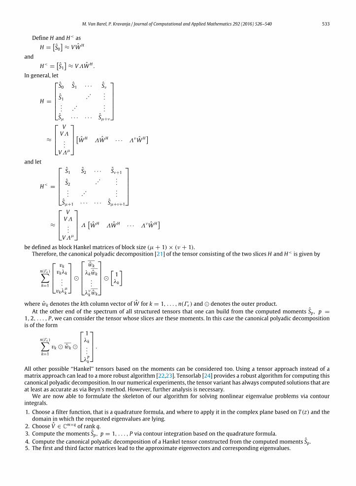
M. Van Barel, P. Kravanja / Journal of Computational and Applied Mathematics 292 (2016) 526–540 533

Define H and H< as

H =S0

≈ VWH

and

H<=

S1

≈ VΛWH .

In general, let

H =

S0 S1 · · · Sν

S1 . .. ...

... . .. ...

Sµ · · · · · · Sµ+ν

≈

VVΛ...

VΛµ

WH ΛWH

· · · ΛνWH

and let

H<=

S1 S2 · · · Sν+1

S2 . .. ...

... . .. ...

Sµ+1 · · · · · · Sµ+ν+1

≈

VVΛ...

VΛµ

ΛWH ΛWH

· · · ΛνWH

be defined as block Hankel matrices of block size (µ + 1) × (ν + 1).Therefore, the canonical polyadic decomposition [21] of the tensor consisting of the two slices H and H< is given by

n(Γϵ )k=1

vk

vkλk...

vkλµ

k

⊙

wk

λkwk...

λνkwk

⊙

1λk

where wk denotes the kth column vector of W for k = 1, . . . , n(Γϵ) and ⊙ denotes the outer product.At the other end of the spectrum of all structured tensors that one can build from the computed moments Sp, p =

1, 2, . . . , P , we can consider the tensor whose slices are these moments. In this case the canonical polyadic decompositionis of the form

n(Γϵ )k=1

vk ⊙ wk ⊙

1λk...

λPk

.

All other possible ‘‘Hankel’’ tensors based on the moments can be considered too. Using a tensor approach instead of amatrix approach can lead to a more robust algorithm [22,23]. Tensorlab [24] provides a robust algorithm for computing thiscanonical polyadic decomposition. In our numerical experiments, the tensor variant has always computed solutions that areat least as accurate as via Beyn’s method. However, further analysis is necessary.

We are now able to formulate the skeleton of our algorithm for solving nonlinear eigenvalue problems via contourintegrals.1. Choose a filter function, that is a quadrature formula, and where to apply it in the complex plane based on T (z) and the

domain in which the requested eigenvalues are lying.2. Choose V ∈ Cm×q of rank q.3. Compute the moments Sp, p = 1, . . . , P via contour integration based on the quadrature formula.4. Compute the canonical polyadic decomposition of a Hankel tensor constructed from the computed moments Sp.5. The first and third factor matrices lead to the approximate eigenvectors and corresponding eigenvalues.

534 M. Van Barel, P. Kravanja / Journal of Computational and Applied Mathematics 292 (2016) 526–540

Fig. 3. Singular values of S0 and S1 . (For interpretation of the references to colour in this figure legend, the reader is referred to the web version of thisarticle.)

6. Numerical experiment

We have tested our algorithm on several linear, polynomial and nonlinear eigenvalue problems. Instead of presentingan overview of these experiments, we consider only one example and choose different scenarios to solve this nonlineareigenvalue problem. We consider the gun problem from the collection of nonlinear eigenvalue problems established byBetcke, Higham, Mehrmann, Schroeder and Tisseur [25]. This problem is related to a model of a radio-frequency gun cavity.The problem size is equal tom = 9956 whereas the function T has the following form:

T (z) =K M iW1 iW2

1

−z√z

√z − α

where K ,M , W1 and W2 are sparse matrices, and α = (108.8774)2.

Wewould like to approximate all the eigenvalues located inside the circle that is symmetric with respect to the real axis,and that intersects the real axis at α = (108.8774)2 and β = 3402.

We choose Γ as the unit circle and N = 32.What is a good choice for the centre µ and the radius ρ such that we can apply the theory to T (µ + ρz)?Let us consider different strategies.

Scenario 1. In this case, we choose the parameters µ and ρ such that z = −3.1 is mapped to the branch point α and suchthat the point z = 2 is mapped to the point β .

z |b0(z)| µ+ρz−3.1 ≈ 10−16 α

2 ≈ 10−10 β

Because the convergence radius r of R(z) is equal to 3.1 and

|b0(r)| ≈ 10−16

the R(z) part does not influence (up to machine precision) the computation of S0 and S1. In other words,

S0 =

n(C)k=1

vkwHk V b0(λk),

S1 =

n(C)k=1

vkwHk Vλkb0(λk)

up to machine precision. This is indicated by the singular values of S0 and S1 shown in Fig. 3. One can clearly observe thedifferent |b0(λk)| levels/sizes. Note that the difference between the blue and red dots gives an indication of the modulus ofthe corresponding eigenvalue.

M. Van Barel, P. Kravanja / Journal of Computational and Applied Mathematics 292 (2016) 526–540 535

Fig. 4. Relative residuals for the computed eigenvalues.

Fig. 5. Coefficients of R(z).

By computing the canonical polyadic tensor decompositionwith 23 terms,we obtain an approximation of 23 eigenvalues.The relative residual for each of the computed eigenvalues λk with corresponding eigenvector vk is given by

ϵk =∥T (λk)vk∥1

∥T (λk)∥1∥vk∥1.

Fig. 4 plots these relative residuals. Because the accuracy of λk depends on the extraction of the corresponding informationfrom S0 and S1, this accuracy is limited to |b0(λk)|. Hence, we expect that

ϵk|b0(λk)| ≈ |b0(r)|.Let us check that

∥Rα∥ ≈ γ

1r

α

where r = 3.1 is the expected convergence radius of R(z) =

α≥0 Rαzα . One can approximate the norms ∥Rα∥ by using theFast Fourier Transform.We are not giving the details here. The results shown in Fig. 5 imply that the computed convergenceradius r ≈ 2.55. We miss an eigenvalue λ⋆ having the following properties;

|b0(λ⋆)| ≈ 10−13

536 M. Van Barel, P. Kravanja / Journal of Computational and Applied Mathematics 292 (2016) 526–540

Fig. 6. Eigenvalues. (For interpretation of the references to colour in this figure legend, the reader is referred to the web version of this article.)

Fig. 7. Singular values of S0 and S1 .

and

|λ⋆| ≈ 2.58 ≈ r.

The two filled red dots in Fig. 6 indicate α and β . The red circle represents the eigenvalue λ⋆ that is missed, while the otherblue circles represent the computed eigenvalues λk. Let us try another scenario.Scenario 2. In this case, we choose the parameters µ and ρ such that z = −2 is mapped to the branch point α and such thatthe point z = 2 is mapped to the point β .

z |b0(z)| µ+ρz−2 ≈ 10−10 α

2 ≈ 10−10 β

The convergence radius r of R(z) now equals r = 2 and

|b0(r)| ≈ 10−10.

M. Van Barel, P. Kravanja / Journal of Computational and Applied Mathematics 292 (2016) 526–540 537

Fig. 8. Relative residuals for the computed eigenvalues.

Fig. 9. Coefficients of R(z).

In the computation of the moments S0 and S1 the R(z) term now comes in with size of order 10−10. Fig. 7 shows the singularvalues of S0 and S1. By computing the canonical polyadic tensor decomposition with 24 terms, we obtain an approximationof 24 eigenvalues. Fig. 8 plots the relative residuals.

Let us check that

∥Rα∥ ≈ γ

1r

α

where r = 2 is the convergence radius of R(z) =

α≥0 Rαzα . The results shown in Fig. 9 imply that r ≈ 2. Note that R0 is ofthe order 10−5 which explains why we get smaller values of the relative residual in Fig. 8. Comparing Figs. 6 and 10 one canobserve that we have found the missing eigenvalue. However, the accuracy of this eigenvalue will be small. To derive thiseigenvalue with high accuracy, we consider the following strategy.

Scenario3. Let us consider a filter function having the following property: the eigenvalues that are lying in the neighbourhoodof a branch point have a larger value of the modulus of the filter function compared to the ‘‘classical’’ filter functions.

Consider, for example, the filter function developed by Hale, Higham and Trefethen [26] to handle the branch point z = 0of

√z. A plot of the modulus of this filter function is shown in Fig. 11.

538 M. Van Barel, P. Kravanja / Journal of Computational and Applied Mathematics 292 (2016) 526–540

Fig. 10. Eigenvalues.

Fig. 11. Plot of the log of the modulus of the filter function developed by Hale, Higham and Trefethen.

The transformation parameters µ and ρ are determined such that

z |b0(z)| µ+ρz−0.05 ≈ 10−16 α

10 ≈ 10−7 β

The singular values of S0 and S1 are shown in Fig. 12.By computing the canonical polyadic tensor decompositionwith 40 terms,we obtain an approximation of 40 eigenvalues.

Fig. 13 plots the relative residuals. Note that this particular filter function allows to compute the eigenvalues in theneighbourhood of the branch point α with a higher accuracy compared to Scenario 2, see Fig. 14.

7. Conclusion

In this paper, we have shown that the accuracy of the computed eigenvalues and eigenvectors using contour integral‘‘measurements’’ of the resolvent not only depends on the eigenvalues inside the contour Γ but also on the eigenvalueconfiguration outside the contour Γ where they are not completely filtered away by the filter function. In contrast to linear

M. Van Barel, P. Kravanja / Journal of Computational and Applied Mathematics 292 (2016) 526–540 539

Fig. 12. Singular values of S0 and S1 .

Fig. 13. Relative residuals for the computed eigenvalues.

and polynomial eigenvalue problems with nonsingular highest degree coefficient, the convergence radius of the R-termin the expression for the resolvent plays also a crucial role in assessing the accuracy of the computed eigenvalues. Thisconvergence radius is determined by the points z in the neighbourhood of the contour Γ for which T (z) is not analytic.In the third scenario we have used a rational filter function that allows to approximate eigenvalues very accurately in theneighbourhood of a branch point of T (z). In future research,wewould like to develop an algorithm that designs good rationalfilters given the region in which one wants to approximate the eigenvalues accurately as well as the points in which T (z)exhibits non analytic behaviour.

Acknowledgements

The research was partially supported by the Research Council KU Leuven, project OT/10/038 (Multi-parameter modelorder reduction and its applications), PF/10/002 Optimization in Engineering Centre (OPTEC), by the Fund for ScientificResearch–Flanders (Belgium), G.0828.14N (Multivariate polynomial and rational interpolation and approximation), and bythe Interuniversity Attraction Poles Programme, initiated by the Belgian State, Science Policy Office, Belgian Network DYSCO(Dynamical Systems, Control, and Optimization). The scientific responsibility rests with its author(s).

540 M. Van Barel, P. Kravanja / Journal of Computational and Applied Mathematics 292 (2016) 526–540

Fig. 14. Eigenvalues.

References

[1] P. Kravanja, M. Van Barel, Computing the Zeros of Analytic Functions, in: Lecture Notes in Mathematics, vol. 1727, Springer, 2000.[2] L.M. Delves, J.N. Lyness, A numerical method for locating the zeros of an analytic function, Math. Comp. 21 (1967) 543–560.[3] A.P. Austin, P. Kravanja, L.N. Trefethen, Numerical algorithms based on analytic function values at roots of unity, SIAM J. Numer. Anal. 52 (2) (2014)

1795–1821.[4] T. Sakurai, H. Sugiura, A projection method for generalized eigenvalue problems using numerical integration, J. Comput. Appl. Math. 159 (2003)

119–128.[5] T. Ikegami, T. Sakurai, U. Nagashima, A filter diagonalization for generalized eigenvalue problems based on the Sakurai–Sugiura projection method,

J. Comput. Appl. Math. 233 (2010) 1927–1936.[6] H. Ohno, Y. Kuramashi, T. Sakurai, H. Tadano, A quadrature-based eigensolver with a Krylov subspace method for shifted linear systems for Hermitian

eigenproblems in lattice QCD, JSIAM Lett. 2 (2010) 115–118.[7] T. Ikegami, T. Sakurai, Contour integral eigensolver for non-Hermitian systems: A Rayleigh–Ritz-type approach, Taiwanese J. Math. 14 (3A) (2010)

825–837.[8] T. Sakurai, H. Tadano, CIRR: A Rayleigh–Ritz type method with contour integral for generalized eigenvalue problems, Hokkaido Math. J. 36 (2007)

745–757.[9] E. Polizzi, Density-matrix-based algorithms for solving eigenvalue problems, Phys. Rev. B 79 (2009) 115112.

[10] L. Krämer, E. Di Napoli, M. Galgon, B. Lang, P. Bientinese, Dissecting the FEAST algorithm for generalized eigenproblems, J. Comput. Appl. Math. 244(2013) 1–9.

[11] P.T.P. Tang, E. Polizzi, FEAST as a subspace iteration eigensolver accelerated by approximate spectral projection, SIAM J. Matrix Anal. Appl. 35 (2)(2014) 354–390.

[12] S.E. Laux, Solving complex band structure problems with the FEAST eigenvalue algorithm, Phys. Rev. B 86 (2012) 075103.[13] S. Güttel, E. Polizzi, P.T.P. Tang, G. Viaud, Zolotarev quadrature rules and load balancing for the FEAST eigensolver, MIMS EPrint 2014.39, Manchester

Institure for Mathematical Sciences, The University of Manchester, July 2014.[14] S. Yokota, T. Sakurai, A projection method for nonlinear eigenvalue problems using contour integrals, JSIAM Lett. 5 (2013) 41–44.[15] J. Asakura, T. Sakurai, H. Tadano, T. Ikegami, K. Kimura, A numerical method for nonlinear eigenvalue problems using contour integrals, JSIAM Lett. 1

(2009) 52–55.[16] J. Asakura, T. Sakurai, H. Tadano, T. Ikegami, K. Kimura, A numerical method for polynomial eigenvalue problems using contour integrals, Japan J.

Indust. Appl. Math. 27 (2010) 73–90.[17] W.-J. Beyn, An integral method for solving nonlinear eigenvalue problems, Linear Algebra Appl. 436 (2012) 3839–3863.[18] M.V. Keldysh, On the characteristic values and characteristic functions of certain classes of non-self-adjoint equations, Dokl. Akad. Nauk 77 (1951)

11–14.[19] M.V. Keldysh, The completeness of eigenfunctions of certain classes of nonselfadjoint linear operators, Uspekhi Mat. Nauk 26 (4160) (1971) 15–41.[20] A.P. Austin, L.N. Trefethen, Computing eigenvalues of real symmetric matrices with rational filters in real arithmetic, SIAM J. Sci. Comput. 37 (2015)

A1365–A1387.[21] T.G. Kolda, B.W. Bader, Tensor decompositions and applications, SIAM Rev. 51 (3) (2009) 455–500.[22] J.M. Papy, L. De Lathauwer, S. Van Huffel, Exponential data fitting usingmultilinear algebra: the decimative case, J. Chemom. 23 (7–8) (2009) 341–351.[23] J.M. Papy, L. De Lathauwer, S. Van Huffel, Exponential data fitting using multilinear algebra: the single-channel and the multi-channel case, Numer.

Linear Algebra Appl. 12 (8) (2005) 809–826.[24] L. Sorber, M. Van Barel, L. De Lathauwer, Tensorlab v2.0, January 2014. URL: http://www.tensorlab.net.[25] T. Betcke, N.J. Higham, V.Mehrmann, C. Schröder, F. Tisseur, NLEVP: A collection of nonlinear eigenvalue problems,MIMS EPrint 2011.116,Manchester

Institute for Mathematical Sciences, The University of Manchester, December 2011.[26] N. Hale, N.J. Higham, L.N. Trefethen, Computing Aα , log(A), and related matrix functions by contour integrals, SIAM J. Numer. Anal. 46 (5) (2008)

2505–2523.