Hilbert Spaces from Path Integrals

Fay Dowker, Steven Johnston, Rafael D. Sorkin

May 31, 2010

Abstract

It is shown that a Hilbert space can be constructed for a quantum

system starting from a framework in which histories are fundamental.

The Decoherence Functional provides the inner product on this “History

Hilbert space”. It is also shown that the History Hilbert space is the

standard Hilbert space in the case of non-relativistic quantum mechanics.

1 Introduction

It is not yet known how quantum theory and gravity will be reconciled. How-ever, the four-dimensional nature of reality revealed by our best theory of grav-ity, General Relativity, suggests that unity in physics will only be achieved ifquantum theory can be founded on the concept of history rather than that ofstate. The same suggestion emerges even more emphatically from the causal setprogramme, whose characteristic kind of spatio-temporal discreteness militatesstrongly against any dynamics resting on the idea of Hamiltonian evolution.

A major step toward a histories-based formulation of quantum mechanicswas taken by Dirac and Feynman, showing that the quantum-mechanical propa-gator can be expressed as a sum over histories [1, 2, 3], but it remains a challengeto make histories the foundational basis of quantum mechanics. One attemptto do this was made by J. Hartle who set out new, histories-based axioms forGeneralised Quantum Mechanics (GQM) which do not require the existence ofa Hilbert space of states [4, 5]. Closely related in its technical aspects — whilstdiffering in interpretational aspiration — is Quantum Measure Theory (QMT)[6, 7, 8, 9]. Thus far, both these approaches appear in the literature more asformal axiomatic systems than as fully fledged mathematical physics, althoughsome concrete examples going beyond ordinary quantum mechanics have beenstudied.[10]

In this paper we take a step toward establishing Quantum Measure The-ory and Generalised Quantum Mechanics more firmly on their foundations andconnecting them up with the more familiar formalism of state-vectors and oper-ators. First we demonstrate in detail the Gel’fand-Naimark-Segal (GNS) typeconstruction given in [10] of a History Hilbert space for any quantum measuresystem (to be defined). It is technically helpful within quantum measure the-ory that such a construction is available, but the conceptual significance of this

1

fact would be slight, were it not that the constructed Hilbert space provably isthe usual Hilbert space in the case of certain familiar quantum systems (via anisomorphism that obtains formally in any unitary quantum theory with pure ini-tial state). In this paper we exhibit non-relativistic particle quantum mechanicsin d spatial dimensions as a quantum measure system, and we prove that theHilbert space constructed from the quantum measure is the usual Hilbert spaceof (equivalence classes of) square integrable complex functions on Rd, givencertain conditions on the propagator. The class of systems for which these con-ditions can be established is large and includes the free particle and the simpleharmonic oscillator. Thus, one of the main ingredients of text-book CopenhagenQuantum Mechanics is derivable from the starting point of histories.

2 Quantum Measure Theory: a histories-based

framework

We describe here the framework set out in [6, 7, 8, 9]. In Quantum MeasureTheory, a physical, quantum system is associated with a sample space Ω ofpossible histories, the space over which the integration of the path integral takesplace. Each history γ in the sample space represents as complete a description ofphysical reality as is classically conceivable in the theory. The kind of elementsin Ω varies from theory to theory. In n-particle quantum mechanics, a historyis a set of n trajectories. In a scalar field theory, a history is a real or complexfunction on spacetime. The business of discovering the appropriate sample spacefor a particular theory is part of physics. Even in the seemingly simple case ofnon-relativistic particle quantum mechanics, we do not yet know what propertiesthe trajectories in Ω should possess, not to mention the knotty problems involvedin defining Ω for fermionic field theories for example. We will be able to sidestepthese issues in the current work.

2.1 Event Algebra

Once the sample space has been settled upon, any proposition about physicalreality is represented by a subset of Ω. For example in the case of the non-relativistic particle, if R is a region of space and T a time, the proposition “theparticle is in R at time T ” corresponds to the set of all trajectories which passthrough R at T . We follow the standard terminology of stochastic processesand refer to such subsets of Ω as events.

An event algebra on a sample space Ω is a non-empty collection, A, of subsetsof Ω such that

1. For any α ∈ A, we have Ω \ α ∈ A.

2. For any α, β ∈ A, we have α ∪ β ∈ A.

An event algebra is then an algebra of sets [11]. It follows immediately that∅ ∈ A, Ω ∈ A (∅ is the empty set) and A is closed under finite unions andintersections.

2

An event algebra A is a Boolean algebra under intersection (logical “and”),union (logical “or”) and complement (logical “not”) with unit element Ω andzero element ∅. It is also a (unital) ring with identity element Ω, multiplicationas intersection and addition as symmetric difference (logical “xor”):

1. α · β := α ∩ β.

2. α+ β := (α \ β) ∪ (β \ α).

This ring is Boolean since α · α = α. It is also an algebra over Z2. Morediscussion of the event algebra is given in [9].

An example of an event algebra is the power set 2Ω := S : S ⊆ Ω of allsubsets of Ω. For physical systems with an infinite sample space, however, theevent algebra will be strictly contained in the power set of Ω, something whichis familiar from classical measure theory1 where the collection of “measurablesets” is not the whole power set.

If A is also closed under countable unions and intersections then A is aσ-algebra.

2.2 Decoherence Functional

A decoherence functional on an event algebra A is a map D : A × A → C suchthat

1. For all α, β ∈ A, we have D(α, β) = D(β, α)∗ (Hermiticity).

2. For all α, β, γ ∈ A with β∩γ = ∅, we haveD(α, β∪γ) = D(α, β)+D(α, γ)(Linearity).

3. D(Ω,Ω) = 1 (Normalisation).

4. For any finite collection of events αi ∈ A (i = 1, . . . , N) the N ×N matrixD(αi, αj) is positive semidefinite (Strong positivity).

A decoherence functional D satisfying the weaker condition D(α, α) ≥ 0 forall α ∈ A is called positive. Note that in Generalised Quantum Mechanics, adecoherence functional is defined to be positive rather than strongly positive[4, 5].

A quantal measure on an event algebra A is a map µ : A → R such that

1. For all α ∈ A, we have µ(α) ≥ 0 (Positivity).

2. For all mutually disjoint α, β, γ ∈ A, we have

µ(α ∪ β ∪ γ) − µ(α ∪ β) − µ(β ∪ γ)− µ(α ∪ γ) + µ(α) + µ(β) + µ(γ) = 0 .

(Quantal Sum Rule)

1To contrast with quantum measure theory, the usual textbook measure theory (see Hal-mos, [11]) will be called “classical”.

3

3. µ(Ω) = 1 (Normalisation).

If D : A × A → C is a decoherence functional then the map µ : A → R

defined by µ(α) := D(α, α) is a quantal measure.A triple, (Ω,A, D), of sample space, event algebra and decoherence functional

will be called a quantum measure system.

2.3 A Hilbert Space Construction

Given a quantum measure system, (Ω,A, D), we can construct a Hilbert space:a complex vector space with (non-degenerate) Hermitian inner product whichis complete with respect to the induced norm. This construction is given in [10]and is essentially that given by V.P. Belavkin in [12, Theorem 3, Part 1] wherethe decoherence functional is called a “correlation kernel”. The constructionis akin to the GNS construction of a Hilbert space from a C∗-algebra and isthe same as the construction appearing in Kolmogorov’s Dilation Theorem [13,Theorem 2.2], [14].

To start, we first construct the free vector space on A and use the decoherencefunctional to define a degenerate inner product on it.

2.3.1 Inner product space: H1

To define the free vector space on an event algebra A we start with the set of allcomplex-valued functions on A which are non-zero only on a finite number ofevents. This set becomes a vector space,H1, if addition and scalar multiplicationare defined by:

1. For all u, v ∈ H1 and α ∈ A, we have (u+ v)(α) := u(α) + v(α).

2. For all u ∈ H1, λ ∈ C and α ∈ A, we have (λu)(α) := λu(α).

We now define an inner product space (H1, 〈·, ·〉1) by defining a degenerateinner product on H1 using the decoherence functional D. For u, v ∈ H1 define:

〈u, v〉1 :=∑

α∈A

∑

β∈A

u(α)∗D(α, β)v(β). (2.1)

This sum is well-defined because u and v are non-zero for only a finite number ofevents. This satisfies the conditions for an inner product. Note that the strongpositivity of the decoherence functional is essential for 〈u, u〉1 ≥ 0.

To see that the inner product is degenerate consider, for example, the non-zero vector u ∈ H1 defined by:

u(x) :=

1 if x = α,1 if x = β,

−1 if x = α ∪ β,0 otherwise

(2.2)

for two nonempty, disjoint events α, β ∈ A. By applying the properties of thedecoherence functional we see that ||u||1 = 0.

4

2.3.2 Hilbert space: H2

We now quotient and complete the inner product space (H1, 〈·, ·〉1) to form aHilbert space (H2, 〈·, ·〉2).

For two Cauchy sequences un, vn in H1 we define an equivalence relation

un ∼1 vn ⇐⇒ limn→∞

||un − vn||1 = 0. (2.3)

We denote the ∼1 equivalence class of a Cauchy sequence un by [un]1. Theset of these equivalence classes form a Hilbert space, (H2, 〈·, ·〉2), if addition,scalar multiplication and the inner product are defined by:

1. For all [un]1, [vn]1 ∈ H1, we have [un]1 + [vn]1 := [un + vn]1.

2. For all [un]1 ∈ H1 and λ ∈ C, we have λ[un]1 := [λun]1.

3. For all [un]1, [vn]1 ∈ H1, we have

〈[un]1, [vn]1〉2 := limn→∞

〈un, vn〉1 (2.4)

These are all well-defined, independent of which representative is chosen fromthe equivalence classes.

The construction of a Hilbert space (here (H2, 〈·, ·〉2)) from an inner productspace (here (H1, 〈·, ·〉1)) is a standard operation described in many textbooks(for example, [15, Section 7], [16, p198]).

Whether or not H2 is separable depends on the particular event algebraand decoherence functional that are used in its construction2. In Sections 3,4 and 4.5 we shall present systems for which the constructed Hilbert space isisomorphic to a separable Hilbert space (the standard Hilbert space for thesystem). In these examples the constructed Hilbert space is therefore separable.

Note that we did not use the full structure of the quantum measure system:only the event algebra, A and the decoherence functional D were used andnowhere did the underlying sample space enter into the game. This will beimportant in our discussion of particle quantum mechanics where there is anevent algebra A but we have no precise definition, as yet, of the sample space.

We will refer to the Hilbert space, H2, constructed from a quantum mea-sure system as the History Hilbert space. For quantum systems which have astandard, Copenhagen formulation in terms of unitary evolution on a Hilbertspace of states and which can also be cast into the form of a quantum measuresystem, the question arises as to the relationship between the standard Hilbertspace and the History Hilbert space. This is the question under study in thispaper and it will be shown that in general the answer depends on the initialstate and the Schrodinger dynamics for the system since these are what definethe decoherence functional. However, we conjecture that generically where bothHilbert spaces exist and the decoherence functional encodes a pure initial state,

2The dimension of H1 is equal to the cardinality of A but the dimension of H2, which isless than that of H1, depends on the ∼1 equivalence relation (which in turn depends on D).

5

they are isomorphic. Moreover the isomorphism is physically meaningful, sothat one can conclude that the History Hilbert space is the standard Hilbertspace of the system.

We will prove this conjecture for a variety of non-relativistic particle systemsand exhibit the isomorphism explicitly. The systems considered include a par-ticle with a finite configuration space, a free non-relativistic particle in d spatialdimensions, and a non-relativistic particle in various backgrounds, including aquadratic potential and an infinite potential barrier. Before turning to thesespecific cases, we recall the following simple lemma.

Lemma 1. A linear map f : HA → HB from a Hilbert space (HA, 〈·, ·〉A) to aHilbert space (HB, 〈·, ·〉B) that preserves the inner product, i.e.

〈f(u), f(v)〉B = 〈u, v〉A (2.5)

for all u, v ∈ HA, is one-to-one.

Proof. For all u, v ∈ HA we have

f(v) = f(u) ⇐⇒ 0 = ||f(u) − f(v)||B = ||f(u− v)||B = ||u− v||A ⇐⇒ u = v(2.6)

3 Finite Configuration Space

We analyse the case of a unitary quantum system with finite configuration spaceas a warm up for the system of main interest, particle quantum mechanics. Con-sider a system which has a finite configuration space of n possible configurationsat any time. We shall only consider the system’s configuration at a finite numberN of fixed times t1 = 0 < t2 < . . . < tN = T . An example of such a system is aparticle with n possible positions at each time which evolves in N − 1 discretetime-steps from time t = 0 to time t = T .

3.1 Standard Hilbert space approach

The Hilbert space for the system is (Cn, 〈·, ·〉) and states of the system at aparticular time are represented by vectors in Cn. For a state ψ ∈ Cn the ith

component, ψi, is the amplitude that the system is in configuration i. For allψ, φ ∈ C

n the non-degenerate inner product is given by

〈ψ, φ〉 :=n∑

i=1

ψ∗i φi. (3.1)

There exists a time evolution operator, U(t′, t), a unitary transformationwhich evolves states at time t to states at time t′ and which satisfies the foldingproperty

U(t′′, t′)U(t′, t) = U(t′′, t) . (3.2)

6

3.2 A Quantum Measure System

Each history, γ, of the system is represented by an N -tuple of integers γ =(γ1, γ2, . . . , γN ) (with 1 ≤ γa ≤ n for all a = 1, . . . , N) where each integer γa

denotes the configuration of the system at time t = ta. The system’s samplespace, Ω, is the (finite) collection of these nN possible histories. The eventalgebra, A, is the power set of Ω: A := 2Ω = S : S ⊆ Ω.

To define the decoherence functional we assume there is an initial stateψ ∈ Cn of unit norm. This can be thought of as a vector in Cn or simply as ann-tuple of amplitudes weighting each initial configuration at time t = 0. Thedecoherence functional for singleton events is,

D(γ, γ) := ψ(γ1)∗U∗

γ2γ1U∗

γ3γ2. . . U∗

γN γN−1(3.3)

δγN γNUγN γN−1

. . . Uγ2γ1ψ(γ1) (3.4)

where γ, γ ∈ Ω, ψ(γ1) is the γ1-th component of ψ and Uγ2γ1is short hand for

U(t2, t1)γ2γ1, the amplitude to go from γ1 at t1 to γ2 at t2. D has “Schwinger-

Kel’dysh” form, equalling the complex conjugated amplitude of γ times theamplitude of γ when the two histories end at the same final position, and zerootherwise. The decoherence functional of events α, β ∈ A is then fixed by thebi-additivity property:

D(α, β) :=∑

γ∈α

∑

γ∈β

D(γ, γ) . (3.5)

We define the restricted evolution of the initial state ψ ∈ Cn with respect toa history γ to be the state ψγ ∈ C

n given by:

ψγ := P γNU(tN , tN−1)PγN−1 · · ·P γ3U(t3, t2)P

γ2U(t2, t1)Pγ1ψ (3.6)

where P i is the projection operator in Cn that projects onto the state which isnon-zero only on the ith configuration. [Thus ψγ is just the configuration γN

weighted by the amplitude UγNγN−1. . . Uγ2γ1

ψ(γ1).] Restricted evolution of theinitial state with respect to an event α is then defined to be the state ψα ∈ Cn

ψα :=∑

γ∈α

ψγ . (3.7)

Note that ψγ = ψγ, so we can use either notation when an event is a singleton.It is easy to see that the decoherence functional for two events α, β ∈ A is equalto the inner product between the two restricted evolution states, ψα and ψβ :

D(α, β) := 〈ψα, ψβ〉. (3.8)

3.3 Isomorphism

We now look at conditions on the initial state and evolution of the system thatensure the History Hilbert space (H2, 〈·, ·〉2) is isomorphic to (Cn, 〈·, ·〉).

7

For this system both the sample space and event algebra are finite so theinner product space (H1, 〈·, ·〉1) is finite dimensional and therefore complete butwith a degenerate inner product. In this case there is no need to consider Cauchysequences of elements of H1 — indeed all Cauchy sequences are eventually con-stant. Instead, we define the equivalence relation directly on H1: u ∼1 v if||u − v||1 = 0. And H2 is defined as H2 := H1/ ∼1 the space of equivalenceclasses, [u]1 under ∼1. For all u, v ∈ H1, we have by (3.8)

〈[u]1, [v]1〉2 := 〈u, v〉1. (3.9)

It will prove useful to define a map f0 : H1 → Cn given by

f0(u) :=∑

α∈A

u(α)ψα, (3.10)

for all u ∈ H1. This sum is well-defined since u(α) is non-zero for only a finitenumber of α ∈ A. This f0 is linear and, for all u, v ∈ H1, we have

〈f0(u), f0(v)〉 = 〈u, v〉1, (3.11)

which ensures[u]1 = [v]1 =⇒ f0(u) = f0(v). (3.12)

Using the map f0 we define the candidate isomorphism f : H2 → Cn by

f([u]1) := f0(u), (3.13)

for all [u]1 ∈ H2. By (3.12), f is well-defined, independent of the equivalenceclass representative chosen. The map f is linear and (3.9) and (3.11) ensurethat for all [u]1, [v]1 ∈ H2, we have:

〈f([u]1), f([v]1)〉 = 〈[u]1, [v]1〉2. (3.14)

By Lemma 1, since f is linear and satisfies (3.14), it is one-to-one. If wecan find a condition on the initial state and dynamics that ensures the map fis onto then it is the isomorphism we seek.

Theorem 1 (Onto). Let the evolution operators U(t′, t) and initial state ψ ∈ Cn

be such that, for each configuration j = 1, . . . , n at the final time, there exists ahistory ending at j, γj = (γj

1 , γj2 , . . . , γ

jN−1, j) ∈ Ω, with non-zero amplitude. In

other words, the j-th component of the restricted evolution of the initial statewith respect to history γj is non-zero: (ψγj )j 6= 0. Then the map f is onto.

Proof. For each j choose a history γj ∈ A such that (ψγj )j 6= 0 (note that ψγj

is only non-zero in the j-th component). Let φ ∈ Cn be a vector we wish tomap to.

Define u ∈ H1 by

u(x) :=

φj/(ψγj )j if x = γj for j = 1, . . . , n,0 otherwise.

(3.15)

This is a well-defined vector in H1 and satisfies f([u]1) = φ. Hence f is onto.

8

An example of a case in which H2 is not isomorphic to Cn is if the initialstate has support only on a single configuration, k, and the evolution is trivial,U(t, t′) = 1. Then the only configuration at the final time with nonzero ampli-tude is k and the History Hilbert space is one dimensional, not Cn. Anotherexample is if the evolution is “local” on the lattice, so that after the first timestep, only k and k ± 1 say have nonzero amplitude. Then the dimension of theHistory Hilbert space will depend on the number of time steps and will growwith N until it reaches n after which it will be constant.

4 Particle in d dimensions

We turn now to a less trivial system, that of a non-relativistic particle movingin d dimensions.

4.1 Hilbert space approach

We recall some basic technology in order to fix our notation. The Hilbert spacefor the system is (L2(Rd), 〈·, ·〉). In order to define this, we first define theinner product space (L2(Rd), 〈·, ·〉0), the space of square integrable functionsψ : Rd → C. For all ψ, φ ∈ L2(Rd) a degenerate inner product is given by

〈ψ, φ〉0 :=

∫

Rd

ψ∗(x)φ(x)dx. (4.1)

To see that the inner product is degenerate consider any vector ψ ∈ L2(Rd)which is non-zero only on a set of measure zero. Although ψ 6= 0, we have||ψ||0 = 0.

For two vectors ψ, φ ∈ L2(Rd) define the equivalence relation ∼ by

ψ ∼ φ ⇐⇒ ||ψ − φ||0 = 0. (4.2)

The ∼ equivalence class of ψ ∈ L2(Rd) will be denoted by [ψ]. The set of allequivalence classes forms the Hilbert space (L2(Rd), 〈·, ·〉) where, for all [ψ], [φ] ∈L2(Rd), 〈[ψ], [φ]〉 := 〈ψ, φ〉0. State vectors for the particle at a fixed time arevectors in L2(Rd).

4.2 Quantum Measure System

The sample space of the system, Ω, is the set of all continuous3 maps γ : [0, T ] →Rd. These maps represent the trajectory of the particle from an initial time t = 0to a final “truncation time” t = T .

3We choose continuous maps for definiteness but recognise that the correct sample spacemay have more refined continuity conditions or even be something more general. The resultsof our work will remain applicable so long as the actual event algebra contains a subalgebraisomorphic to the A we define here and on which the measure is defined by the propagator inthe same — standard — way.

9

Introducing a truncation time T seems necessary for the construction under-taken below, which produces the quantal measure for the corresponding subal-gebra AT ⊆ A. This limitation to a subalgebra of the full event algebra is onlyapparent, however, because A is the union of the AT , and the measure of anevent A ∈ A does not depend on which subalgebra we refer it to. In section 4.6we explain this in detail for the case of unitary theories such as we are concernedwith in the present paper.

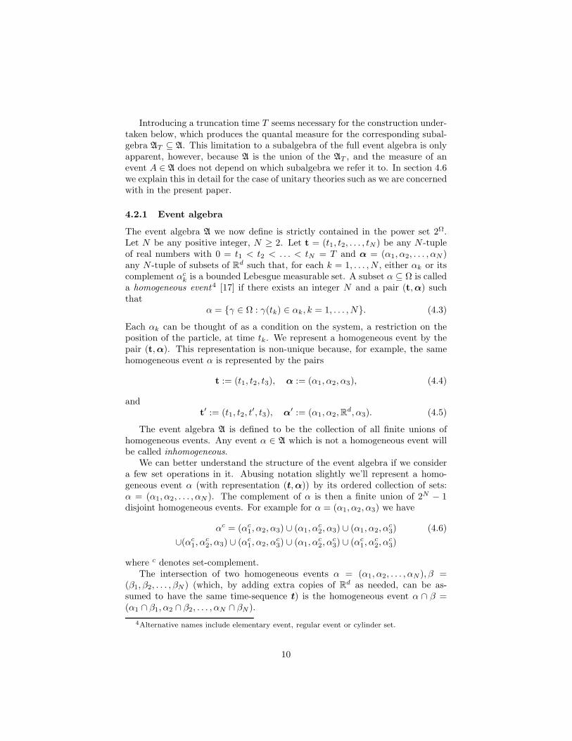
4.2.1 Event algebra

The event algebra A we now define is strictly contained in the power set 2Ω.Let N be any positive integer, N ≥ 2. Let t = (t1, t2, . . . , tN ) be any N -tupleof real numbers with 0 = t1 < t2 < . . . < tN = T and α = (α1, α2, . . . , αN )any N -tuple of subsets of Rd such that, for each k = 1, . . . , N , either αk or itscomplement αc

k is a bounded Lebesgue measurable set. A subset α ⊆ Ω is calleda homogeneous event4 [17] if there exists an integer N and a pair (t,α) suchthat

α = γ ∈ Ω : γ(tk) ∈ αk, k = 1, . . . , N. (4.3)

Each αk can be thought of as a condition on the system, a restriction on theposition of the particle, at time tk. We represent a homogeneous event by thepair (t,α). This representation is non-unique because, for example, the samehomogeneous event α is represented by the pairs

t := (t1, t2, t3), α := (α1, α2, α3), (4.4)

andt′ := (t1, t2, t

′, t3), α′ := (α1, α2,Rd, α3). (4.5)

The event algebra A is defined to be the collection of all finite unions ofhomogeneous events. Any event α ∈ A which is not a homogeneous event willbe called inhomogeneous.

We can better understand the structure of the event algebra if we considera few set operations in it. Abusing notation slightly we’ll represent a homo-geneous event α (with representation (t,α)) by its ordered collection of sets:α = (α1, α2, . . . , αN ). The complement of α is then a finite union of 2N − 1disjoint homogeneous events. For example for α = (α1, α2, α3) we have

αc = (αc1, α2, α3) ∪ (α1, α

c2, α3) ∪ (α1, α2, α

c3) (4.6)

∪(αc1, α

c2, α3) ∪ (αc

1, α2, αc3) ∪ (α1, α

c2, α

c3) ∪ (αc

1, αc2, α

c3)

where c denotes set-complement.The intersection of two homogeneous events α = (α1, α2, . . . , αN ), β =

(β1, β2, . . . , βN ) (which, by adding extra copies of Rd as needed, can be as-sumed to have the same time-sequence t) is the homogeneous event α ∩ β =(α1 ∩ β1, α2 ∩ β2, . . . , αN ∩ βN ).

4Alternative names include elementary event, regular event or cylinder set.

10

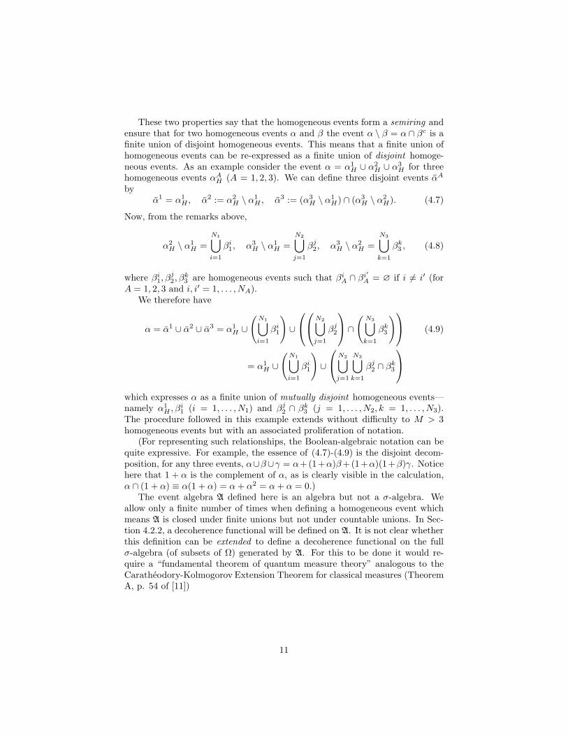
These two properties say that the homogeneous events form a semiring andensure that for two homogeneous events α and β the event α \ β = α ∩ βc is afinite union of disjoint homogeneous events. This means that a finite union ofhomogeneous events can be re-expressed as a finite union of disjoint homoge-neous events. As an example consider the event α = α1

H ∪ α2H ∪ α3

H for threehomogeneous events αA

H (A = 1, 2, 3). We can define three disjoint events αA

byα1 = α1

H , α2 := α2H \ α1

H , α3 := (α3H \ α1

H) ∩ (α3H \ α2

H). (4.7)

Now, from the remarks above,

α2H \ α1

H =

N1⋃

i=1

βi1, α3

H \ α1H =

N2⋃

j=1

βj2, α3

H \ α2H =

N3⋃

k=1

βk3 , (4.8)

where βi1, β

j2, β

k3 are homogeneous events such that βi

A ∩ βi′

A = ∅ if i 6= i′ (forA = 1, 2, 3 and i, i′ = 1, . . . , NA).

We therefore have

α = α1 ∪ α2 ∪ α3 = α1H ∪

(

N1⋃

i=1

βi1

)

∪

N2⋃

j=1

βj2

∩

(

N3⋃

k=1

βk3

)

(4.9)

= α1H ∪

(

N1⋃

i=1

βi1

)

∪

N2⋃

j=1

N3⋃

k=1

βj2 ∩ β

k3

which expresses α as a finite union of mutually disjoint homogeneous events—namely α1

H , βi1 (i = 1, . . . , N1) and βj

2 ∩ βk3 (j = 1, . . . , N2, k = 1, . . . , N3).

The procedure followed in this example extends without difficulty to M > 3homogeneous events but with an associated proliferation of notation.

(For representing such relationships, the Boolean-algebraic notation can bequite expressive. For example, the essence of (4.7)-(4.9) is the disjoint decom-position, for any three events, α∪β∪γ = α+(1+α)β+(1+α)(1+β)γ. Noticehere that 1 + α is the complement of α, as is clearly visible in the calculation,α ∩ (1 + α) ≡ α(1 + α) = α+ α2 = α+ α = 0.)

The event algebra A defined here is an algebra but not a σ-algebra. Weallow only a finite number of times when defining a homogeneous event whichmeans A is closed under finite unions but not under countable unions. In Sec-tion 4.2.2, a decoherence functional will be defined on A. It is not clear whetherthis definition can be extended to define a decoherence functional on the fullσ-algebra (of subsets of Ω) generated by A. For this to be done it would re-quire a “fundamental theorem of quantum measure theory” analogous to theCaratheodory-Kolmogorov Extension Theorem for classical measures (TheoremA, p. 54 of [11])

11

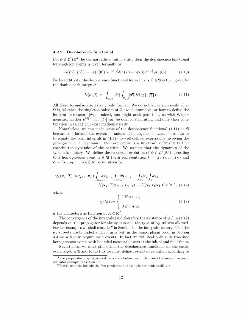
4.2.2 Decoherence functional

Let ψ ∈ L2(Rd) be the normalised initial state, then the decoherence functionalfor singleton events is given formally by

D(γ, γ) := ψ(γ(0))∗e−iS[γ]δ(γ(T ) − γ(T ))eiS[γ]ψ(γ(0)) . (4.10)

By bi-additivity, the decoherence functional for events α, β ∈ A is then given bythe double path integral:

D(α, β) :=

∫

γ∈α

[dγ]

∫

γ∈β

[dγ]D(γ, γ) . (4.11)

All these formulae are, as yet, only formal. We do not know rigorously whatΩ is, whether the singleton subsets of Ω are measureable, or how to define theintegration-measure [dγ]. Indeed, one might anticipate that, as with Wienermeasure, neither eiS[γ] nor [dγ] can be defined separately, and only their com-bination in (4.11) will exist mathematically.

Nonetheless, we can make sense of the decoherence functional (4.11) on A

because the form of the events — unions of homogeneous events — allows usto equate the path integrals in (4.11) to well-defined expressions involving thepropagator a la Feynman. The propagator is a function5 K(x′, t′|x, t) thatencodes the dynamics of the particle. We assume that the dynamics of thesystem is unitary. We define the restricted evolution of ψ ∈ L2(Rd) accordingto a homogeneous event α ∈ A (with representation t = (t1, t2, . . . , tN ) andα = (α1, α2, . . . , αN )) to be ψα given by

ψα(xT , T ) := χαN(xT )

∫

αN−1

dxN−1

∫

αN−2

dxN−2 · · ·

∫

α2

dx2

∫

α1

dx1

K(xT , T |xN−1, tN−1) · · ·K(x2, t2|x1, 0)ψ(x1), (4.12)

where

χA(x) :=

1 if x ∈ A,

0 if x /∈ A.(4.13)

is the characteristic function of A ⊂ Rd.The convergence of the integrals (and therefore the existence of ψα) in (4.12)

depends on the propagator for the system and the type of αk subsets allowed.For the examples we shall consider6 in Section 4.4 the integrals converge if all theαk subsets are bounded and, it turns out, in the isomorphism proof in Section4.3 we will only require such events. In fact we will deal only with two-timehomogeneous events with bounded measurable sets at the initial and final times.

Nevertheless we must still define the decoherence functional on the entireevent algebra A and to do this we must define restricted evolution according to

5The propagator may in general be a distribution, as in the case of a simple harmonicoscillator example in Section 4.4.

6These examples include the free particle and the simple harmonic oscillator.

12

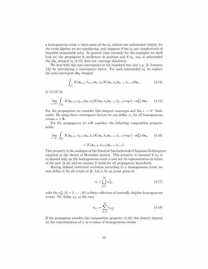
a homogeneous event α when some of the αk subsets are unbounded (which, forthe event algebra we are considering, only happens if the αk are complements ofbounded measurable sets). In general (and certainly for the examples we shalllook at) the propagator is oscillatory in position and if αk, say, is unboundedthe dxk integral in (4.12) does not converge absolutely.

We deal with this non-convergence in the standard way (see e.g. [2, footnote13]) by introducing a convergence factor. For each unbounded αk we replacethe non-convergent dxk integral

∫

αk

K(xk+1, tk+1|xk, tk)K(xk, tk|xk−1, tk−1)dxk, (4.14)

in (4.12) by

limǫ→0+

∫

αk

K(xk+1, tk+1|xk, tk)K(xk, tk|xk−1, tk−1) exp(

−ǫx2k

)

dxk. (4.15)

For the propagators we consider this integral converges and the ǫ → 0+ limitexists. By using these convergence factors we can define ψα for all homogeneousevents α ∈ A.

For the propagators we will consider, the following composition propertyholds:

limǫ→0+

∫

Rd

K(xk+1, tk+1|xk, tk)K(xk, tk|xk−1, tk−1) exp(

−ǫx2k

)

dxtk(4.16)

= K(xk+1, tk+1|xk−1, tk−1).

This property is the analogue of the Einstein-Smoluchowski-Chapman-Kolmogorovequation in the theory of Brownian motion. This property is essential if ψα isto depend only on the homogeneous event α and not its representation in termsof the pair (t,α) and we assume it holds for all propagators henceforth.

Having defined restricted evolution according to a homogeneous event wenow define it for all events in A. Let α be an event given by

α =

M⋃

k=1

αkH , (4.17)

with the αkH (k = 1, . . . ,M) a finite collection of mutually disjoint homogeneous

events. We define ψα as the sum

ψα :=

M∑

k=1

ψαkH. (4.18)

If the propagator satisfies the composition property (4.16) this doesn’t dependon the representation of α as a union of homogeneous events.

13

We can now define the decoherence functional for the system. For two eventsα, β ∈ A and an initial normalised vector ψ ∈ L2(Rd) we define the decoherencefunctional D : A × A → C by

D(α, β) := 〈ψα, ψβ〉0 . (4.19)

This can be shown to be equal to (4.11) using the familiar expression for thepropagator K as a path integral

K(x2, t2|x1, t1) =

∫

[dγ]eiS[γ] (4.20)

where the integral is over all paths γ which begin at x1 at t1 and end at x2 att2.

4.3 Isomorphism

Henceforth we assume the initial state ψ ∈ L2(Rd) has unit norm, the deco-herence functional for events in A is given by the propagator K as described insection 4.2.2, the spaces H1, H2 are defined as in sections 2.3.1 and 2.3.2, andthe maps f0 and f are defined as in section 4.3. We will find conditions on theinitial state and propagator that ensure the History Hilbert space (H2, 〈·, ·〉2) isisomorphic to (L2(Rd), 〈·, ·〉).

It will prove useful to define a map f0 : H1 → L2(Rd) given by

f0(u) :=∑

α∈A

u(α) [ψα] , (4.21)

for all u ∈ H1. The sum is well-defined since u(α) is only non-zero for a finitenumber of events α ∈ A. This map f0 is linear and for all u, v ∈ H1, we have

〈f0(u), f0(v)〉 = 〈u, v〉1. (4.22)

Since the map f0 is linear and preserves the inner products in H1 and L2(Rd)it maps a Cauchy sequence, un of elements of H1 to a Cauchy sequence inL2(Rd). Since L2(Rd) is complete this sequence has a limit and it is this limitwe assign as the image of our candidate isomorphism, f : H2 → L2(Rd) definedby:

f([un]1) := limn→∞

f0(un). (4.23)

The map f is linear and well-defined, independent of which representative,un of the [un]1 equivalence class is used in the definition above.

Using (4.22) and the continuity of the 〈·, ·〉 inner product [20, Lemma 3.2-2]we have

〈f([un]1), f([vn]1)〉 := 〈 limn→∞

f0(un), limm→∞

f0(vm)〉

= limn→∞

〈f0(un), f0(vn)〉 = limn→∞

〈un, vn〉1 =: 〈[un]1, [vn]1〉2. (4.24)

By Lemma 1, since f is linear and satisfies (4.24), it is one-to-one. We cannow state our main theorem:

14

Theorem 2 (Onto). Let the propagator K(xT , T |x0, 0) be continuous as afunction of (xT ,x0) ∈ R2d and such that for each xT , ∃x0 with K(xT , T |x0, 0)non-zero. Then the map f defined by (4.23) is onto.

To prove Theorem 2 we follow a strategy suggested by the proof of Theorem1: we want to show, roughly, that every final position can be reached by a historyof nonzero amplitude. The implementation of the strategy is more complicatedthan in the finite case and will proceed by establishing a series of Lemmas.

Lemma 2. Let the propagator K(xT , T |x0, 0) be continuous as a function of(xT ,x0) ∈ R2d. Let ψ ∈ L2(Rd) be the initial state. Let A ⊂ Rd be a compactmeasurable set and α be the homogeneous event represented by t = (0, T ),α =(A,Rd). Then

ψα(xT , T ) :=

∫

A

K(xT , T |x0, 0)ψ(x0)dx0, (4.25)

is continuous as a function of xT ∈ Rd.

Proof. Fix a position xT ∈ Rd at the final time. Let C be the closed unit ballcentred at xT . By assumption, K(xT , T |x0, 0) is continuous (as a function of(xT ,x0) ∈ R2d) so, by the Heine-Cantor theorem, it is uniformly continuous (asa function of (xT ,x0)) on the compact set C × A ⊂ R2d. This means for anyǫ > 0 there exists δ > 0 such that for (xT ,x0), (x

′T ,x

′0) ∈ C ×A we have

√

|xT − x′T |

2 + |x0 − x′0|

2 < δ =⇒ |K(xT , T |x0, 0) −K(x′T , T |x

′0, 0)| < ǫ.

(4.26)In particular if x0 = x′

0 and |xT − x′T | < δ < 1 then

∣

∣

∣K(xT , T |x0, 0) −K(x′T , T |x0, 0)

∣

∣

∣ < ǫ ∀x0 ∈ A . (4.27)

So for |xT − x′T | < δ < 1 we have

|ψα(xT , T ) − ψα(x′T , T )|

:=

∣

∣

∣

∣

∫

A

(

K(xT , T |x0, 0) −K(x′T , T |x0, 0)

)

ψ(x0)dx0

∣

∣

∣

∣

≤

(∫

A

∣

∣

∣K(xT , T |x0, 0) −K(x′T , T |x0, 0)

∣

∣

∣

2

dx0

)12(∫

A

|ψ(x0)|2dx0

)12

< ǫ|A|

where we have used the Cauchy-Schwarz inequality and the normalisation ofψ and |A| is the Lebesgue measure of A. |A| is finite so, since ǫ is arbitrary,ψα(xT , T ) is continuous at xT . This holds for any xT ∈ Rd.

Lemma 3. Let the propagator K(xT , T |x0, 0) be continuous as a function of(xT ,x0) and be such that for each xT , ∃x0 s.t. K(xT , T |x0, 0) is non-zero. Thenfor any point xT ∈ Rd at the truncation time t = T there exists a compact

15

measurable set A ⊂ Rd (depending on xT ) such that the homogeneous event αrepresented by t = (0, T ),α = (A,Rd) satisfies

ψα(xT , T ) :=

∫

A

K(xT , T |x0, 0)ψ(x0)dx0 6= 0. (4.28)

Proof. The proof relies on Lebesgue’s Differentiation Theorem [19, p100] whichstates that if G : Rd → C is an integrable function then

G(x) = limB→x

∫

BG(x′)dx′

|B|, (4.29)

for almost all x ∈ Rd. Here B is an d-dimensional ball centred on x whichcontracts to x in the limit and |B| is its Lebesgue measure.

Aiming for a contradiction we assume that∫

A

K(xT , T |x′, 0)ψ(x′)dx′ = 0, (4.30)

for all compact measurable sets A ⊂ Rd.Taking A to be a sequence of closed balls contracting to an arbitrary point

x ∈ Rd at the initial time then (4.29) gives

K(xT , T |x, 0)ψ(x) = limA→x

∫

AK(xT , T |x

′, 0)ψ(x′)dx′

|A|= 0, (4.31)

for almost all x ∈ Rd. This is a contradiction since K is continuous and ∃x0

with K(xT , T |x0, 0) 6= 0 so there is a compact set containing x0 on whichK(xT , T |x, 0) 6= 0.

Lemma 4. Let the propagator K(xT , T |x0, 0) satisfy the conditions of Lemma3. Then, for any point xT ∈ Rd at the truncation time there exists a homoge-neous event α represented by t = (0, T ),α = (A,B) (with A ⊂ Rd a compactmeasurable set and B ⊂ R

d an open ball centred on xT ) and a strictly positivereal number P such that ψα is uniformly continuous in B and |ψα(x, T )| > Pfor all x ∈ B.

Proof. By Lemmas 2 and 3, there exists a compact measurable set A ⊂ Rd suchthat, for the homogeneous event β represented by β = (A,Rd) the functionψβ(x, T ) is continuous for all x ∈ Rd and satisfies ψβ(xT , T ) 6= 0.

This implies there exists δ > 0 such that

|x − xT | < δ =⇒ |ψβ(x, T ) − ψβ(xT , T )| <|ψβ(xT , T )|

2. (4.32)

Let B be the open ball of radius δ centred on xT . Setting P = |ψβ(xT , T )|/2 > 0we see that x ∈ B implies |ψβ(x, T )| > P > 0.

Since ψβ(x, T ) is continuous it is uniformly continuous in any compact setand therefore any subset of a compact set. It is thus uniformly continuous inB. For α := (A,B) we then have ψα = χBψβ (χB is the characteristic functionof B) and the result follows.

16

The next lemma is the heart of the proof.

Lemma 5. Let the propagatorK(xT , T |x0, 0) satisfy the conditions of Lemmas2 and 3. Let I be a compact d-interval with positive measure |I| > 0 at thetruncation time. Then for any ǫ > 0 there exists a vector u ∈ H1 such that

||[χI ] − f0(u)|| < ǫ . (4.33)

Proof. Let ǫ > 0. For any x ∈ I there exists, by Lemma 4, a homogeneousevent αx represented by αx = (Ax, Bx) (with Bx an open ball centred on x)and a real number Px > 0 such that ψαx

is uniformly continuous in Bx and|ψαx

(x′, T )| > Px for all x′ ∈ B.The collection of Bx, taken for all x ∈ I, form an open cover of I, which,

since I is compact, admits a finite subcover labelled by xi ∈ I | i = 1 . . .N.Define Ai := Axi

, Bi := Bxi, αi := αxi

and Pi := Pxi.

Each Bi will now be “cut up” into finitely many disjoint sets, Dij , over whichthe ψαi

functions vary by only “small amounts”. The first step toward this isto form a finite number of N mutually disjoint sets Ci ⊆ Bi given by

C1 := B1 ∩ I, Ci := (Bi ∩ I) \

i−1⋃

j=1

Cj (i = 2, . . . , N), (4.34)

and such that

I =N⋃

i=1

Ci. (4.35)

Without loss of generality we assume the Ci are non-empty.Each function ψαi

is uniformly continuous in Ci and satisfies |ψαi(x, T )| > Pi

for all x ∈ Ci for some strictly positive Pi ∈ R.Let P > 0 be the minimum value of the Pi and let δi > 0 (i = 1, . . . , N) be

chosen such that

|x − y| < δi =⇒ |ψαi(x, T ) − ψαi

(y, T )| <ǫP√

|I|, (4.36)

for all x,y ∈ Ci.Letting δ > 0 be the minimum of the δi now subdivide each Ci into a finite

number, Mi, of non-empty disjoint sets Dij (i = 1, . . . , N ; j = 1, . . . ,Mi) suchthat

Mi⋃

j=1

Dij = Ci and x,y ∈ Dij =⇒ |x − y| < δ. (4.37)

If we arbitrarily choose points xij ∈ Dij the Dij sets are “small enough”

that, by (4.36), |ψαi(xij , T ) − ψαi

(x, T )| < ǫP/√

|I| for all x ∈ Dij . Defininghomogeneous events αij to be represented by αij := (Ai, Dij) therefore gives∣

∣

∣

∣

1 −ψαij

(x, T )

ψαij(xij , T )

∣

∣

∣

∣

=|ψαij

(xij , T ) − ψαij(x, T )|

|ψαij(xij , T )|

<1

|ψαij(xij , T )|

ǫP√

|I|<

ǫ√

|I|,

(4.38)

17

for all x ∈ Dij where we note |ψαij(xij)| > P > 0.

Now define a H1 vector by

u(x) :=

1/ψαij(xij , T ) if x = αij for i = 1, . . . , N ; j = 1, . . . ,Mi

0 otherwise.(4.39)

This is a well-defined vector in H1 since there are only a finite number ofevents x = αij on which u(x) is non-zero. We now compute

||[χI ] − f0(u)||2 =

∫

Rd

∣

∣

∣

∣

∣

∣

χI(x) −

N∑

i=1

Mi∑

j=1

ψαij(x, T )

ψαij(xij , T )

∣

∣

∣

∣

∣

∣

2

dx (4.40)

=

N∑

i=1

Mi∑

j=1

∫

Dij

∣

∣

∣

∣

1 −ψαij

(x, T )

ψαij(xij , T )

∣

∣

∣

∣

2

dx <

N∑

i=1

Mi∑

j=1

∫

Dij

ǫ2

|I|dx = ǫ2,

where we have used (4.38), the disjointness of the Dij and

N∑

i=1

Mi∑

j=1

∫

Dij

dx = |I|. (4.41)

We have thus constructed u ∈ H1 such that

||[χI ] − f0(u)|| < ǫ. (4.42)

We can now prove Theorem 2.

Proof. (of Theorem 2)A step function on Rd is a function S : Rd → C that is a finite linear

combination of characteristic functions of compact d-intervals.Let [φ] ∈ L2(Rd) be the element we wish to map to. We assume [φ] 6= 0

for otherwise the zero vector in H2 would satisfy f(0) = [φ]. Let [Sn] bea sequence of L2(Rd) vectors, where the Sn are step functions that are notidentically zero, such that

||[φ] − [Sn]|| <1

2n, (4.43)

for each positive integer n. Such a sequence [Sn] exists since the step functionsare dense in L2(Rd) [19, p133].

For each step function Sn we can (non-uniquely) decompose it as

Sn =

Nn∑

i=1

sn,iχIn,i, (4.44)

18

for a finite collection of Nn ≥ 1 non-zero complex numbers sn,i and mutuallydisjoint compact d-intervals In,i. Define Mn > 0 to be the maximum value of|sn,i| (i = 1, . . . , Nn).

By Lemma 5, for each n = 1, 2, . . . and each i = 1, . . . , Nn there exists avector un,i ∈ H1 such that

||[χIn,i] − f0(un,i)|| <

1

2nNnMn. (4.45)

Defining un ∈ H1 by

un :=

Nn∑

i=1

sn,iun,i, (4.46)

we see that

||[Sn]−f0(un)|| ≤

Nn∑

i=1

|sn,i|||[χIn,i]−f0(un,i)|| <

Nn∑

i=1

|sn,i|

2nNnMn<

Nn∑

i=1

1

2nNn=

1

2n.

(4.47)This, together with (4.43), implies

||[φ] − f0(un)|| <1

n, (4.48)

i.e. f0(un) is a Cauchy sequence converging to [φ]. Since f0 preserves theinner product this means un is a Cauchy sequence of H1 elements such thatf([un]1) = [φ]. [φ] ∈ L2(Rd) was arbitrary so the map f is onto.

Theorem 2 gives sufficient conditions on the propagator for the HistoryHilbert space to be isomorphic to L2(Rd) for any initial state. If the initialstate itself satisfies certain conditions, then the conditions on the propagatorcan be relaxed. For example, if the initial state, ψ, is everywhere nonzero, theneven a trivial evolution with a delta-function propagator will suffice to make theHistory Hilbert space isomorphic to L2(Rd).

4.4 Examples

We now look at examples for which the propagator is known explicitly. Theexpressions for the propagators are taken from [21].

For a free particle of mass m in d dimensions the Lagrangian is

L =m

2x2. (4.49)

The propagator is given by

K(x′, t′|x, t) =

(

m

2πi~(t′ − t)

)d/2

exp

[

im

2~(t′ − t)(x′ − x)2

]

. (4.50)

19

For a charged particle (with mass m and charge e) in a constant vector potentialA the Lagrangian is

L =m

2x2 + eA · x. (4.51)

The propagator is given by

K(x′, t′|x, t) =

(

m

2πi~(t′ − t)

)d/2

exp

[

im

2~(t′ − t)(x′ − x)2 +

ieA

~· (x′ − x)

]

.

(4.52)Both of these propagators satisfy the conditions for Theorem 2. Since the sys-tem with constant vector potential is gauge equivalent to the free particle, thetheorem is bound to hold for both or neither.

A particle of massm in a simple harmonic oscillator potential of period 2π/ωin one spatial dimension has Lagrangian

L =m

2x2 −

mω2

2x2 . (4.53)

Defining, ∆t := t′ − t, the propagator is

K(x′, t′|x, t) =

(

mω

2πi~ sin(ω∆t)

)1/2

exp

[

−mω

2i~

[

(x′2 + x2) cot(ω∆t) − 2xx′

sin(ω∆t)

]]

,

(4.54)if ∆t 6= Mπ/ω for integer M . If ∆t = Mπ/ω for integer M we have

K(x′, t′|x, t) = e(−iMπ/2)δ(x′ − (−1)Mx). (4.55)

Clearly the propagator fulfils the conditions for Theorem 2 if the truncationtime T is not equal toMπ/ω for integerM . More care is needed if the truncationtime is an integer multiple of π/ω.

If T = Mπ/ω for integerM then the propagator does not fulfil the conditionsfor Theorem 2. In this case we cannot use only two-time events to demonstratethe isomorphism. The Hilbert spaces are still isomorphic, however, as can beseen by using three-time homogeneous events α represented by α = (R, αt2 , αT )in which the set at time t1 = 0 is R and such that T − t2 is not an integermultiple of π/ω. Evolving the initial state according to these events is equiv-alent to unrestrictedly evolving the initial state from t1 = 0 to t2 > 0. Thestate at time t2 can then be viewed as the “initial state” for two-time homoge-neous events represented by (αt2 , αT ). The conditions for Theorem 2 are metby K(xT , T |xt2 , t2) so the theorem can be applied and the isomorphism demon-strated. These ideas can similarly be applied to the simple harmonic oscillatorin d dimensions.

4.5 Particle with an infinite potential barrier

Consider a physical system of a non-relativistic particle in one dimension re-stricted to the positive halfline R

+ = x ∈ R|x > 0 by an infinite potentialbarrier.

20

The Hilbert space for this system is L2(R+) which we define as a vectorsubspace of L2(R):

L2(R+) := [ψ] ∈ L2(R) : ψ(x) = 0 for x ≤ 0. (4.56)

The sample space, Ω, and event algebra, A, for this system will be thesame as for a particle in 1 dimension. The difference is that, when definingthe decoherence functional we now use an initial vector ψ ∈ L2(R) such thatψ(x) = 0 for x ≤ 0 and a propagator defined by [22, p40]:

K(x′, t′|x, t) = χR+(x′)χR+(x)

(

m

2πi~(t′ − t)

)1/2

(4.57)

×

[

exp

[

im(x′ − x)2

2~(t′ − t)

]

− exp

[

im(x′ + x)2

2~(t′ − t)

]]

,

where m is the mass of the particle.This propagator does not satisfy the conditions of Theorem 2—it is con-

tinuous as a function of (x, x′) ∈ R2 but is zero for x ≤ 0 or x′ ≤ 0. It isnot surprising therefore that the map f : H2 → L2(R) defined by (4.23) isnot an isomorphism with this event algebra and decoherence functional, namelybecause f only gives vectors [ψ] ∈ L2(R+) as expected.

It is possible to show, by using the same methods used in the isomorphismproof for a particle in d dimensions, that the History Hilbert space for this eventalgebra and decoherence functional is isomorphic to L2(R+).

4.6 Infinite times

In the preceding sections we assumed a finite time interval both in the finiteconfiguration space case and the quantum mechanics case. We can extend theanalysis to cover all times to the future of the initial time, t ∈ [0,∞). We willdescribe how to do this in the quantum mechanics case; the extension can beapplied, mutatis mutandis, to the finite configuration space case.

The sample space Ω is now the set of continuous real functions on [0,∞). Thehomogeneous events, α, are defined as before as represented by a positive integerN ≥ 1, an N -tuple of times t = (t1 = 0, t2, . . . tN ) and an N -tuple of measurablesubsets of Rd, α = (α1, α2, . . . , αN ) such that either αk or αc

k is bounded. Now,however, there is no truncation time and therefore no restriction on the timestk, they can be arbitrarily large. The event algebra, A, is the set of finite unionsof the homogeneous events. Since there is no common truncation time T , therestricted evolution of the initial state with respect to a homogeneous event, asdefined by 4.12, results in a state defined at a time, tN , that depends on theevent. Such states cannot be added together to define the restricted evolution ofthe initial state with respect to a event which is a union of disjoint homogeneousevents which have different last times. Instead, we evolve the restricted stateback to the initial time t = 0, i.e. we define

ψα(x0, 0) :=

∫

Rd

dxNK(x0, 0|xN , tN )ψα(xN , tN ) (4.58)

21

for each homogeneous event α.We can now work at the initial time. The restricted state at t = 0 of an

inhomogeneous event is the sum of the restricted states at t = 0 of its con-stituent disjoint homogeneous events (as in (4.18)). The decoherence functionalis defined as the inner product of the restricted states at t = 0.

The event algebra, A∞, in the infinite time case contains a subalgebra, A∞|T ,which is canonically isomorphic to the event algebra, AT with a truncation timebecause each history with a truncation time corresponds to an event in the in-finite time case: the event is the set of infinite time histories which match thetruncated history. The decoherence functionals on A∞|T and AT agree becausethe unitary evolution back to the initial time preserves the inner product. Theo-rem 2 therefore also applies to the semi-infinite time case: if the History Hilbertspace is isomorphic to L2(Rd) with a truncation time, it is isomorphic without.In the former case it is convenient to construct the History Hilbert space at thetruncation time as we did and in the latter it is convenient to consider the His-tory Hilbert space associated with the initial time, but for the unitary systemswe are considering this is not a real distinction, being akin to working in theSchrodinger or Heisenberg Picture.

4.7 Mixed states

The conjecture made at the end of section 2 was that where both standardand History Hilbert spaces exist, generically they are isomorphic if the decoher-ence functional encodes a pure initial state. If in contrast the initial state is astatistical mixture then the decoherence functional is a convex combination ofdecoherence functionals, and then the History Hilbert space can be bigger thanthe standard Hilbert space. Indeed, we make note of the following expectationsfor the case of a finite configuration space. If the initial state is a density matrixof rank ri then the History Hilbert space is generically the direct sum of ricopies of the standard Hilbert space Cn. Even more generally, if there is also afinal density matrix of rank rf then the History Hilbert space is the direct sumof ri copies of C

rf . [28]

5 Discussion

If histories-based formulations of quantum mechanics are nearer to the truththan state- and operator-based formulations, and in particular if somethinglike Quantum Measure Theory is the right framework for a theory of quantumgravity, then there is no particular reason why one should expect Hilbert spacesto be part of physics at a fundamental level.

Indeed, in histories formulations which assume only plain, “weak” positivity(and in which, therefore, no Hilbert space arises), certain kinds of devices canin principle exist that are not possible within ordinary quantum mechanics, andthis could be regarded as desirable. For example non-signaling correlations ofthe “PR box” type become possible [23].

22

Nor does reference to a Hilbert space seem to be needed for interpretivereasons. On the contrary, attempts to overcome the “operationalist” bias of theso called Copenhagen interpretation tend to lead in the opposite direction, awayfrom state-vectors and toward histories and the associated events [7].

Thus, it seems hard to argue on principle that a Hilbert space is needed.On the other hand, there do exist good reasons to regard strong positivity asmore natural than weak positivity. First, it is mathematically much simplerthan weak positivity, whence more amenable to being verified and worked with[10]. (Not that its definition is any simpler, but that it comprises, apparently,far fewer independent conditions.) Second, strong positivity is preserved un-der composition of subsystems, whereas the obvious “product measure” of twoweakly positive quantal measures is not in general positive at all. And third— at a technical level — the histories hilbert space to which strong positivityleads has already proven to be useful in certain applications [23, 25], while thereare also indications that the map taking events α ∈ A to vectors in H couldbe of aid in the effort to extend the decoherence functional from A to a largerfragment of the σ-algebra it generates.

It thus seems appropriate to add strong positivity to the axioms defininga decoherence functional (as we have done in this paper), and from a stronglypositive decoherence functional a histories hilbert space H automatically arises.Once we have it, we can ask whether the histories hilbert space helps us tomake contact with the quantal formalism of standard textbooks. This is some-thing that any proposed formulation has to be able to do, and it is the principalquestion animating the present paper. The positive answer we have obtained isthat for the systems we have studied, the histories hilbert spaces that pertainto them can be directly identified with the corresponding state-spaces of theordinary quantum description. (The two are “naturally isomorphic”.) Therebyan important part of the mathematical apparatus of ordinary quantum me-chanics is recovered quite simply. This result can be seen as an advance forboth Generalised Quantum Mechanics and Quantum Measure Theory becausethe basic underlying structures — histories and decoherence functionals — arecommon to both approaches. (Strong positivity has not normally been assumedin Generalised Quantum Mechanics, but there is no reason why it could not be.)

Beyond state-vectors, the other main ingredients of the standard quantummachinery are the operators representing position, momentum, field values, “ob-servables”, and the like. How might they be derived from histories? In thespecialized context of unitary, Hamiltonian evolution and the Schrodinger equa-tion, time-ordered operators can be obtained from functions (“functionals”) onthe sample space Ω (see [2]), but whether such a relationship exists in the samegenerality as the histories hilbert space itself (that is for any quantum mea-sure theory) remains to be seen. An interesting generalization where one doesseem able to recover field operators from the decoherence functional is that ofquantum field theory on a causal set [26].

The context of this paper has been that of non-relativistic quantum me-chanics, yet people have not yet completely laid the rigorous mathematicalfoundations of a histories framework for this theory. Nevertheless the decoher-

23

ence functional limited to A × A is known (we haven’t yet defined calculus butwe can calculate the volume of a pyramid, see footnote 10, page 371 of [2]), andthis sufficed to demonstrate our main result, that the History Hilbert space His the standard Hilbert space. A key question for the future that will also beof interpretational significance is what the sample space of histories is. Is it theset of all continuous trajectories and if so, exactly how continuous are they?This is closely related to the question, can the decoherence functional — andhence the quantal measure — be extended to a larger collection of sets thanA? Is that larger collection the whole σ-algebra generated by A or somethingsmaller? These questions have been explored by Geroch [27]. To the extent thatthey find satisfactory answers, we will be able to say that Quantum Mechanicsas Quantum Measure Theory is as well-defined mathematically as the Wienerprocess.

Be that as it may, neither Brownian motion nor the quantum mechanics ofnonrelativistic point-particles can lay claim to fundamental status in present-day physics. Relativistic quantum field theory comes closer, but in that context,neither formulation — neither path-integrals/histories nor state-vectors-cum-operators — enjoys a mathematically rigorous existence. Instead we have thedivergences and other pathologies whose resolution is commonly anticipatedfrom the side of quantum gravity. If this expectation is borne out, the decoher-ence functional of quantum gravity might actually be easier to place on a soundmathematical footing than that of the Hydrogen atom, because in place of apath-integral over an infinite dimensional function-space, we will have somethingmore finitary in nature, like a summation over a discrete space of histories.7

In that case the trek back to nonrelativistic quantum mechanics will belonger, but we expect that the histories hilbert space defined above will still bean important milestone along the way.

The authors would like to thank Chris Isham for helpful criticisms on thefirst draft of this paper. We also thank Raquel S. Garcia for discussions duringthe early stages of this work. SJ is supported by a STFC studentship. FD ac-knowledges support from ENRAGE, a Marie Curie Research Training Networkcontract MRTN-CT-2004-005616 and the Royal Society IJP 2006/R2. FD andSJ thank Perimeter Institute for Theoretical Physics for hospitality during thewriting of this paper. Research at Perimeter Institute for Theoretical Physicsis supported in part by the Government of Canada through NSERC and by theProvince of Ontario through MRI.

7One can already observe such a trend in the theory formulated in [26] of a free scalar fieldon a causal set C corresponding to a bounded spacetime region. The decoherence functional ofthe theory can be computed and is again given by a double integral of the type of (4.11). Nowhowever, the domain of integration is just R

n rather than some infinite-dimensional path-space. Moreover, the integrand contains, besides the expected oscillating phases, dampingterms that lessen by half the need for integrating-factors like those in (4.15).

24

References

[1] P.A.M. Dirac, The Lagrangian in Quantum Mechanics, Phys. Z. Sowjetu-nion, (1933)

[2] R. P. Feynman, Space-Time Approach to Non-Relativistic Quantum Me-chanics, Rev. Mod. Phys, 20, 367 (1948)

[3] R. P. Feynman and A. R. Hibbs, Quantum Mechanics and Path Integrals,McGraw Hill 1965.

[4] J. B. Hartle, The quantum mechanics of cosmology Dec 1989, Lectures atWinter School on Quantum Cosmology and Baby Universes, Jerusalem,Israel, Dec 27, 1989 - Jan 4, 1990.

[5] J. B. Hartle, Spacetime quantum mechanics and the quantum mechanics ofspacetime in Proceedings of the Les Houches Summer School on Gravitationand Quantizations, Les Houches, France, 6 Jul - 1 Aug 1992, eds J. Zinn-Justin, and B. Julia, North-Holland (1995) arXiv:gr-qc/9304006

[6] R.D. Sorkin, Quantum Mechanics as Quantum Measure Theory,Mod.Phys.Lett. A9 (1994) 3119-3128, arXiv:gr-qc/9401003

[7] R.D. Sorkin Quantum Dynamics without the Wave Function, J.Phys. A: Math. Theor. 40 (2007) 3207-3221, arXiv:quant-ph/0610204v1http://www.perimeterinstitute.ca/personal/rsorkin/some.papers/

[8] R.D. Sorkin, Quantum Measure Theory and Its Interpretation, in QuantumClassical Correspondence: Proceedings of the 4th Drexel Symposium onQuantum Nonintegrability, held Philadelphia, September 8-11, 1994, pages229-251 (International Press, Cambridge Mass. 1997) D.H. Feng and B-L Hu, editors, arXiv:gr-qc/9507057

[9] R.D. Sorkin, An exercise in “anhomomorphic logic”, Journal ofPhysics: Conference Series (JPCS) 67 : 012018 (2007), a spe-cial volume edited by L. Diosi, H-T Elze, and G. Vitiello, anddevoted to the Proceedings of the DICE-2006 meeting, heldSeptember 2006, in Piombino, Italia. arXiv:quant-ph/0703276http://www.perimeterinstitute.ca/personal/rsorkin/some.papers/

[10] X. Martin, D. O’Connor and R.D. Sorkin Random walk in generalized quan-tum theory Phys. Rev. D 71, 024029 (2005), arXiv:gr-qc/0403085

[11] P.R. Halmos, Measure Theory, Van Nostrand, 1964.

[12] V.P. Belavkin, Reconstruction theorem for quantum stochastic processes,Translated from: Teoreticheskaya i Matematicheskaya Fizika, 62 (3) 409–431 (1985), arXiv:math/0512410

[13] D. E. Dutkay, Positive definite maps, representations and frames, Reviewsin Mathematical Physics, vol. 16, No. 4 (2004), arXiv:math/0511137

25

[14] D.E. Evans and J.T. Lewis, Dilations of Irreversible Evolutions in AlgebraicQuantum Theory, Dublin Institute for Advanced Studies 1977.

[15] R. Geroch, Special Topics in Particle Physics, Unpublished

[16] K.G. Binmore, The Foundations of Analysis: Book 2, Topological Ideas,Cambridge University Press, 1981.

[17] C.J. Isham, Quantum Logic and the Histories Approach to Quantum The-ory, J.Math.Phys. 35 (1994) 2157-2185, arXiv:gr-qc/9308006.

[18] M. Chaichian, A. Demichev, Path integrals in physics. Vol.1, Stochasticprocesses and quantum mechanics Institute of Physics, Bristol. 2001.

[19] R.L. Wheeden, A. Zygmund, Measure and Integral: An Introduction toReal Analysis, Marcel Dekker, Inc. 1977.

[20] E. Kreyszig, Introductory Functional Analysis with Applications, John Wi-ley & Sons, 1978.

[21] C. Grosche, F. Steiner, Handbook of Feynman Path Integrals, Springer,1998

[22] L.S. Schulman, Techniques and Applications of Path Integration, Wiley-Interscience publication, 1981.

[23] David Craig, Fay Dowker, Joe Henson, Seth Major, David Rideout andRafael D. Sorkin, “A Bell Inequality Analog in Quantum Measure Theory”,J. Phys. A: Math. Theor. 40 : 501-523 (2007), quant-ph/0605008,http://www.perimeterinstitute.ca/personal/rsorkin/some.papers/

[24] Rafael D. Sorkin, “Quantum dynamics without the wave function” J.Phys. A: Math. Theor. 40 : 3207-3221 (2007) (http://stacks.iop.org/1751-8121/40/3207) quant-ph/0610204http://www.perimeterinstitute.ca/personal/rsorkin/some.papers/

[25] Sumati Surya and Petros Wallden, “Quantum Covers in Quantum MeasureTheory” arXiv:0809.1951

[26] Steven Johnston, “Feynman Propagator for a Free Scalar Field on a CausalSet” Phys. Rev. Lett 103 : 180401 (2009) arXiv:0909.0944 [hep-th]

[27] R. Geroch, Path Integrals, Unpublished notes available athttp://physics.syr.edu/ sorkin/lecture.notes/

[28] Marie Ericsson and David Poulin (unpublished)

26