Int. J. Mol. Sci. 2002, 3, 710-732International Journal of

Molecular SciencesISSN 1422-0067

www.mdpi.org/ijms/

Higher Energy Derivatives in Hilbert Space Multi-Reference Coupled Cluster Theory : A ConstrainedVariational Approach

K. R. Shamasundar and Sourav Pal

Physical Chemistry Division, National Chemical Laboratory, Pune, India - 411008.

Tel. 91-20-5890754 Fax. 91-2:0-5893044

E-mail: pal@ems.ncl.res.in

Received: 18 December 2001 / Accepted: 10 April 2002 / Published: 30 June 2002

Abstract: In this paper, we present formulation based on constrained variational ap-

proach to compute higher energy derivatives upto third order in Hilbert Space Multi-

Reference Coupled Cluster (HSMRCC) Theory. This is done through the use of a

functional with Lagrange multipliers corresponding to HSMRCC method, as done by

Helgaker, Jorgensen and Szalay. We derive explicit expressions upto third order en-

ergy derivatives. Using (2n + 1) and (2n + 2) rules, the cancellation of higher order

derivatives of functional parameters that are not necessary according to these rules,

is explicitly demonstated. Simplified expressions are presented. We discuss several

aspects of the functional used and its potential implications.

Keywords: Energy Derivatives; Lagrange Multipliers; Constrained Variation; Hilbert

Space Multi-Reference; Coupled Cluster.

c©2002 by MDPI, Basel, Switzerland. Reproduction for noncommercial purposes permitted.

Int. J. Mol. Sci. 2002, 3 711

1 INTRODUCTION

In last two decades, coupled-cluster (CC) method [1–3] has emerged as the most efficient and

accurate method for calculation of electronic structure and spectra where inclusion of electron

correlation is an important factor. For systems dominated by single determinant, the dynamical

electron correlation is the most important part of correlation. The single-reference coupled-cluster

(SRCC) method compactly sums up several infinite order perturbation terms through the solution

of a non-linear equation leading to an accurate description of dynamical correlation. By its very

method of formulation, the much required property of size-extensivity property is automatically

included in CC method.

Another reason for the emergence of SRCC as state-of-the-art method is development of efficient

analytic energy derivative techniques for the calculation of molecular electronic properties [4, 5].

The linear response theory is the appropriate framework for this [4, 6]. In this theory, molecular

energy gradients, hessians, dipole-moment, polarizability and other frequency dependent proper-

ties appear as energy response quantities of appropriate order in perturbation. Stationary elec-

tronic theories i.e., theories where some or all parameters are determined from stationarity of

energy functional, enjoy an advantage for calculating energy derivatives. Such theories obey the

Hellmann-Feynmann theorem and its generalization (2n + 1) rule, which drastically simplify the

evaluation of energy derivatives [7]. There have been several attempts to formulate a stationary

theory based on coupled-cluster ansatz [11–14]. All such attempts have resulted in theories much

more complicated theories. As a result, the standard CC method is non-stationary.

As a consequence of non-stationary nature of the standard CC method, the calculation of first

order energy response requires that first order response of cluster amplitudes be calculated for every

mode of perturbation. However, Bartlett and co-workers [5, 8] have shown that the requirement

of first derivative of cluster amplitudes for each mode of perturbation can be replaced by a single

perturbation-independent quantity, known as Z-vector. There have been further developments in

obtaining compact expressions for first and second derivatives including orbital response [5, ?, 10].

By constructing an unconstrained Lagrangian functional, Helgaker, Jorgensen and coworkers have

incorporated all such developments in a single formulation which is easily applicable to higher

orders [15–18]

Description of molecular excited states and potential energy surfaces can not be easily done

with single-reference theories such as SRCC. These are the cases which are marked by nearly

equal domination of a number of determinants referred to as quasi-degenerate. This is essen-

tially known as non-dynamical electron correlation, which can be efficiently introduced by using

a multi-determinantal description of zeroth order situation [3, 19, 20]. There have been several

approaches developed in last two decades. Dominant among them is the effective Hamiltonian

Int. J. Mol. Sci. 2002, 3 712

method [21, 22], where an effective Hamiltonian is diagonalized within a suitably chosen quasi-

degenerate model space to approximately reproduce a part of the spectrum associated with the

exact Hamiltonian. Pursuing coupled-cluster ideas have led to two different ansatz for wave op-

erator to introduce dynamical correlation. First is the Fock-Space (FS) multi-reference coupled-

cluster (MRCC) method [19]. It is efficient for studying states associated with a model space

of specified number of of valence electrons, while at the same time considering all lower valence

model spaces with fewer number of electrons in them. This makes it suitable for studying spectro-

scopic quantities such as excitation energies. The second method, Hilbert-Space (HSMRCC) [23],

is useful for study of several interacting states with a fixed number of electrons and is suitable

for potential energy surfaces. To overcome the intruder state problems associated with complete

model spaces usually used in effective Hamiltonian theories several different directions are being

pursued in recent years. Use of incomplete model space [19, 24] intermediate Hamiltonian [21, 25]

and state-specific multi-reference approaches [26, 27] are major ones.

It may be mentioned that the one-valence FSMRCC is equivalent to the Equation of Motion CC

(EOM-CC) method. In the context of EOM-CC fully relaxed analytic response has been developed

and implemented by Gauss and Stanton [28, 29]. However, FSMRCC method for one valence

upward, and HSMRCC in particular, have no parallel in EOM-CC or any other SR based theories.

Thus, it is important to formulate the linear response of effective Hamiltonian MRCC methods [30].

Analytic linear response approach for a general effective Hamiltonian based on coupled-cluster

method was originally formulated by Pal [31]. It has been implemented to the FSMRCC [32].

This has been recently used to calculate dipole-moments of open-shell molecules [33]. Szalay has

outlined an approach [34] based on undetermined Lagrange multipliers method used by Hegaker,

Jorgensen and coworkers in SRCC [15–17], to outline the calculation of first-derivatives of MRCC

methods, and analyze the cost of MRCC derivatives as compared to SRCC derivatives. The

present authors have introduced Z-vector method for effective Hamiltonian MRCC methods and

derived expressions for the first energy derivative for HSMRCC theory [35].

The current work focuses on deriving expressions for higher-order energy derivatives (specifi-

cally, upto third-derivative) for HSMRCC theory through appropriate higher-order generalization

of Z-vector method. For this we propose an undetermined Lagrange multiplier functional which

is similar to the one used by Szalay [34]. The equations for model space coefficients, cluster

amplitudes, Lagrange multipliers and their first derivatives are obtained. In section II, SRCC

and MRCC linear response, Z-vector method and its relation to the method based on contrained

Lagrange multipliers are briefly summarized. Z-vecror method for HSMRCC is also discussed,

outlining its relation to the functional proposed by Szalay. In section III, using a functional

with undetermined Lagrange multipliers corresponding to HSMRCC method leading to Z-vector

equations, expressions upto third derivatives for a specific state are derived. Equations for the

Int. J. Mol. Sci. 2002, 3 713

Lagrange multipliers and its derivatives are presented. Section IV summarizes the results with

some general comments on the results of section III.

2 SRCC AND MRCC LINEAR RESPONSE THEORY

In this section, key developments in SRCC and MRCC linear response theory are discussed. The

relation of Z-vector to constrained variational method is examined in detail. The advantage of

the latter method is highlighted for use in computing higher-order derivatives.

2.1 Single Reference Coupled Cluster Method

The SRCC method has been thoroughly discussed in literature. It is obtained by using expo-

nential ansatz eT acting on a determinant |Φ〉

|Ψ〉 = eT |Φ〉 (1)

in Schrodinger equation

H|Ψ〉 = E|Ψ〉 (2)

where T is the cluster operator with usual second quantized definition.

T =∑i,a

tai aaai +

1

4

∑a,b,i,j

tabij aaabajai + · · · (3)

In the above expression i, j, . . . refer to orbitals occupied in |Φ〉, and a, b, . . . refer to orbitals

unoccupied in |Φ〉 and aa and ai are orbital creation and annihilation operators respectively.

Although T is N -body operator, it is usually truncated. Truncation of T to one and two-body parts

is quite common and referred to as CCSD, although upto four-body truncations have been reported

in literature. By substituting ansatz into equation and premultiplication with e−T followed by

projection with hole-particle determinants |Φab...ij... 〉 (henceforth denoted as |Φq〉 with q denoting

collective hole-particle excitations respect to |Φ〉 ), we get the CC equations.

〈Φ|e−T HeT |Φ〉 = E (4)

〈Φq|e−T HeT |Φ〉 = 0 ,∀ |Φq〉 (5)

The equations for cluster amplitudes are non-linear in nature and can be solved by iteration.

Int. J. Mol. Sci. 2002, 3 714

2.2 Analytic Linear Response for SRCC method.

A computational framework to analytically calculate various properties with SRCC method

was first outlined by Monkhrost using linear response approach [36]. In this framework, various

molecular properties are defined to be various order derivatives of energy with respect to a small

external perturbation strength parameter g. By expanding Energy E, Hamiltonian H and the

cluster amplitudes T as a Taylor series around zero perturbation strength, and collecting terms of

same order in g, expressions for various derivatives of CC Energy can be obtained. For first order,

neglecting orbital response, the equations are,

E(1) = Y tT (1) + Q(g) (6)

AT (1) = B(g) (7)

where,

AT (1) =〈Φq|e−T [H,T (1)]eT |Φ〉 ,∀q

(8)

Y tT (1) = 〈Φ|e−T [H,T (1)]eT |Φ〉 (9)

B(g) =〈Φq|e−T H(1)eT |Φ〉 ,∀q

(10)

Q(g) = 〈Φ|e−T H(1)eT |Φ〉 (11)

In above equations, superscript (1) on T and H refers to first derivative of respective quantities

with respect to external perturbation strength parameter g. Terms within are used to denote

column vectors and superscript t denotes transpose.

Similar equations can be derived for higher derivatives of T and E. Inclusion of orbital response

(which is important for geometric derivatives) was first done by Jorgensen and Simons [37] who

derivided detailed expressions upto second derivatives using the second-quantization framework.

2.3 Z-vector method and other developments

As outlined, SRCC, being non-stationary theory, does not have the advantage of (2n + 1) rule.

Thus, T (1) is required for calculating first derivative of energy E(1). This has to be done for every

mode of perturbation which is a disadvantage. A step towards eliminating this disadvantage was

taken by Bartlett and coworkers [8, 5, 9]. They make use of a technique based on Dalgarno’s

interchange theorem [38] used by Handy and Schaefer for configuration interaction (CI) energy

derivatives [39]. The technique, known as Z-vector technique, derives algebraic expressions for

reducing the number of linear equations for orbital rotations and cluster amplitudes. By inverting

Int. J. Mol. Sci. 2002, 3 715

equation (7) and substituting in (6), E(1) can be reorganized as,

E(1) = ZtB(g) + Q(g) (12)

with Zt,

ZtA = Y T (13)

Equation (13) is a perturbation independent equation providing the Zt vector. The advantage

of such reorganization is, unlike earlier equation (7), equation (13) needs to solved only once. This

Z-vector method is in some sense equivalent to (2n + 1) type of rule for non-stationary methods.

Further simplifications have been carried out by introducing effective CC density matrices [5, 9]

much akin to CI derivative developments. The technique of Rice and coworkers [40] has also been

applied to reduce the number of AO to MO transformations. First applications of CC analytic

derivatives have been reported by Bartlett and coworkers [41] and Scheiner and coworkers [42].

2.4 Method of Undetermined Lagrange Multipliers

The conceptually simple procedure of eliminating T (1) in favor of a Z-vector is somewhat cum-

bersome for higher orders and has been pursued by Salter and coworkers [10]. However, Helgakar,

Jorgensen and coworkers [17], have pursued an attractive alternative formulation of CC derivative

which automatically incorporates Z-vector technique to all orders. Such a formulation proceeds

by constructing a Lagrange functional with undetermined multipliers Λ = λq,∀q corresponding

to CC equations (5) as follows.

J (T, Λ) = 〈Φ|e−T HeT |Φ〉 +∑

q

λq〈Φq|e−T HeT |Φ〉 (14)

The functional may be viewed as approximation to the full Extended Coupled Cluster (ECC)

functional of Arponen [13]. The full ECC functional been used by Pal and coworkers to derive

the first and higher order energy derivatives using a stationary approach [43–45]. Optimization of

functional (14) leads to same equations as cluster amplitude equations (5) and Z-vector equations

(13) with Λ taking the role of Z-vector. In this formulation, it is transparant to derive expressions

for higher order derivatives. While T (1) obey (2n + 1) rule, the undetermined multipliers λ obey

(2n + 2) rule [16].

2.5 Multi-Reference Coupled Cluster (MRCC) Theories.

Extension of coupled-cluster method to quasi-degenerate situations demanding multi-reference

description has been non-trivial. Different approaches were followed by different researchers.

Int. J. Mol. Sci. 2002, 3 716

Among them, the approach of constructing an effective Hamiltonian in a complete model space

has emerged as the standard one [3, 21, 22]. We briefly summarize the approach in the following.

A strongly interacting M -dimensional complete model space is considered by distributing a

given number of electrons among a conveniently chosen set of valence orbitals. This model space,

P0, is assumed to approximate the quasi-degenerate target space P , spanned by M exact states of

exact Hamiltonian H. Hence, it contains the zeroth-order approximations for all the exact states

under consideration. Dynamical correlation is brought in via wave-operator Ω mapping model

and target space as,

P = ΩP0 (15)

The wave-operator, Ω, through an appropriate parametrization, is constructed by solving gener-

alized Bloch equation.

HΩP0 = ΩHΩP0 (16)

Bloch equation is simpliy a restatement of the schrodinger equation for all targeted states. The

exact energy and zeroth order approximations of target states within model space, |Ψ(0)i 〉 , are

obtained by diagonalizing the effective Hamiltonian.

Heff = P0HΩP0 (17)

Two kinds of parametrizations for the wave-operator Ω have been widely discussed in literature.

The first one involves the use of a common reference vaccum |Φ〉 for defining a single second-

quantized cluster operator T connecting model spaces with different number of valence electrons

from zero to a specified number used to build the model space. This leads to Fock-Space MRCC

(FSMRCC) [19]. T is so constructed that the corresponding wave-operator, Ω = eT , is able to

yield exact states for different model spaces connected by T . FSMRCC has been successful in

accurate computations of spectroscopic quantities such as ionization potential, electron affinity,

excitation energies [46, 47].

The second formulation does not use a single reference vaccum, but uses as many vacua as the

number of states in the manifold, with one cluster operator for each vaccum. This is referred to

as Hilbert-Space MRCC (HSMRCC) [23]. Unlike FSMRCC, HSMRCC does not require the use

of model spaces with different number of valence electrons. The wave-operator is written as,

Ω =∑

µ

eTµ|Φµ〉〈Φµ| (18)

where Tµ is the cluster operator with respect to vaccum |Φµ〉 similar in structure to SRCC cluster

operator. Tµ does not contain excitations leading to states within model space. Using the above

Int. J. Mol. Sci. 2002, 3 717

ansatz in equations (16) and (17) and projecting with determinants, |Φq(µ)〉, hole-particle excited

with respect to |Φµ〉 (q denotes collective orbital indices involved in the excitation), we get the

following HSMRCC equations.

〈Φq(µ)|e−TµHeTµ|Φµ〉 −∑

ν

〈Φq(µ)|e−TµeTν |Φν〉Hνµeff = 0 ∀ q, µ (19)

∑µ

HνµeffCµi = EiCνi ∀ν (20)

∑ν

CiνHνµeff = EiCiµ ∀µ (21)

Hνµeff = 〈Φν |e−TµHeTµ|Φµ〉 (22)∑

µ

CiµCµi − 1 = 0 (23)

Ciν and Cµi refer to left and right eigenvectors of the effective Hamiltonian Heff . HSMRCC has

been pursued by various researchers and has been found to be useful for description of potential

energy surfaces [48–50]. Spin adaptated formulations have also been pursued and successfully

applied to various chemical systems [51].

There have been several other MRCC approaches such as Intermediate Hamiltonian approach [21, 25],

use of incomplete model spaces [19, 24] and state-specific MRCC [26, 27]. However, the current

work focuses on complete model space effective Hamiltonian based MRCC approaches with special

emphasis on HSMRCC theory.

2.6 Analytic Linear Response for MRCC Theories

Application of linear response to obtain expressions for MRCC derivatives was initiated by Pal,

who, following Monkhrost’s approach outlined the formulation for the effective Hamiltonian based

MRCC theory [31]. Specific expressions were obtained for one hole, one particle and hole-particle

sectors of FSMRCC theory [32]. The structure of the original nonvariational formulation did

not include prescription of Z-vector and thus were not applicable for higher energy derivatives

and even gradients. Applications of the formalism to compute first order molecular properties

have however been carried out in recent years [33]. The formalism has also been extended to

time-dependent perturbation case [52].

On the other hand, Szalay was the first to extend Helgaker and Jorgensen’s method by proposing

a Lagrangian functional for a chosen state in the manifold which yields MRCC cluster amplitude

and effective Hamiltonian diagonalization equations [34]. His work mainly concerned with esti-

Int. J. Mol. Sci. 2002, 3 718

mating the relative cost of MRCC first order response calculations as compared to SRCC response

equations.

First efforts towards directly introducing Handy-Schefer Z-vector type technique for the ef-

fective Hamiltonian, Heff , were carried out by Pal and coworkers [53]. Working on FSMRCC

response equations for one hole model space, they concluded that only highest sector amplitude

derivatives can be eliminated from Heff(1) under degenerate diagonal Heff . Further work on HSM-

RCC theory has shown that it is not possible to eliminate cluster amplitude derivatives in effective

Hamiltonian first derivative with a single Z-vector for all states, although M2 number of inde-

pendent Z-vectors would be sufficient. Recently, however, the present authors have showed that

it is possible to eliminate the cluster amplitude derivatives for a chosen state energy derivative.

They have derived detailed equations for HSMRCC Z-vector for a chosen state and developed

efficient expressions for HSMRCC energy first derivative by extending the idea of effective CC

density matrices [35].

3 HSMRCC HIGHER ENERGY DERIVATIVES

Extension of algebraic Z-vector method is difficult for higher order energy derivatives, although

it has been pursued in SRCC context by Salter and coworkers [10] to obtain second derivative

expressions. It is advantageous to go over to constrained variation approach [17]. The approach

generalizes the Z-vector method to all orders retaining the simplicity of HSMRCC method. In

this section, we derive expressions for HSMRCC energy derivatives upto third-order for a chosen

state. For this, we propose a functional with Lagrange multipliers corresponding using HSMRCC

equations, (19)-(23), as constraints. The functional leads to equations for Lagrange multipliers

corresponding to cluster amplitude equation (19) to be the same as Z-vector equations derived

recently [35]. Using (2n + 1) rule for cluster amplitudes and model space coefficients, (2n + 2)

rule for Lagrange multipliers, the expressions for second and third order are written in a simple

form.

3.1 The Lagrangian functional and obtaining linear response

Before giving explicit expression for the Lagrangian functional which corresponds to HSMRCC

method, we assume the following abbreviations. We denote the set of cluster amplitudes for all

vacua by T , the set of all model space coefficients for the i-th state by Ci and the set of all La-

grange multpliers corresponding to HSMRCC cluster amplitude equations (19) by Λ. We further

collectively refer the set of quantities T ,Ci,Λ and the energy of i-th state Ei (the Lagrange mul-

tiplier corresponding to biorthogonal conditions (23)), by Θ. The following equations summarize

Int. J. Mol. Sci. 2002, 3 719

the above abreviations.

T = Tµ ∀µ (24)

Ci =

Ciµ, Cµi ∀µ

(25)

Λ = Λµ ∀µ (26)

Θ = T,Ci, Λ, Ei (27)

Now, the Lagrangian functional which corresponds to HSMRCC equations (19)-(23) is constructed

as,

J (Θ) =∑µ,ν

CiνCµiHνµeff +

∑q,η

λq(η)Eq(η)

−Ei

(∑µ

CiµCµi − 1

)(28)

where HSMRCC equation for T , (19), is denoted by Eq(µ) = 0. Making J stationary with

respect to Θ generates sufficient number of equations to determine these parameters. The above

functional is similar to one used by Szalay [34] in context with HSMRCC first derivatives. However,

the present functional does not introduce Ci dependence in second term. As a consequence, Jleads to Z-vector equations derived by eliminating the first order response of cluster amplitudes,

T (1) from energy first derivative expression. Although current formulation results in slightly

complicated expressions for effective CC density matrices, it will be advantageous as discussed in

next section.

To derive expressions for various order derivatives, linear response theory is used. A small

perturbation H(1) with strength parameter g is introduced into the Hamiltonian H as,

H(g) = H + gH(1) (29)

Since Θ is determined at all strenghts of perturbation g, the functional J becomes a function of

g, denoted by J (g,Θ). Response equations can be obtained in two different approaches. First

approach, followed by Helgaker, Jorgensen and coworkers [17] and Bartlett and coworkers [10] is

to expand the functional J and the stationary equations obtained for Θ as a Taylor series in

strength parameter g. Terms of same order in g in Θ equations are collected and equated to

obtain hierarchical equations for various response quantities Θ(n).

Second approach, proposed by Pal [12, 54] in the context with stationary CC theories, is to

derive response equations of any required order as a stationary equations. In this approach,

Int. J. Mol. Sci. 2002, 3 720

J (g,Θ) is expanded as,

J (g,Θ) = J (0) + gJ (1) +1

2!g2J (2) +

1

3!g3J (3) + · · · (30)

It should be noted that J (n) is a functional of quantitiesΘ(m) m = 0, n

. All response equations

upto a required order n can be derived by making the functionals

J (k) k = 0, n

stationary with

respect toΘ(m) m = 0, n (m ≤ k)

. This leads to the following equations.

∂J (k)

∂Θ(m)= 0 ,∀k,∀m, (m ≤ k), (k = 0, n) (31)

This includes the n = 0 case corresponding to the unperturbed (zeroth order) equations as well.

Henceforth, we drop the superscipt for zeroth-order quantities. It has been shown that there is a

large amount of redundancy in the above equations. Hence it is sufficient to solve

∂J (m)

∂Θ= 0 ∀m = 0, n (32)

This leads to hierarchical equations forΘ(m) ∀m = 0, n

. In this work, we follow the second

approach in deriving response equations. According to (2n + 1) rule associated with stationary

methods, we need Θ and Θ(1) to obtain expressions upto thrid order energy derivatives, and hence

equations (32) need to be solved upto n = 1. It should be noted that both approaches are entirely

equivalent and lead to identical equations with a given functional.

3.2 Response response equations upto first order

Detailed expressions for J (n) upto n = 3 are given in Appendix A, equations (A-4)-(A-6). To

derive response equations for Θ upto first order, we use expression for J along with equation

(A-1). Zeroth-Order quantities, Θ, can be obtained by

∂J∂Θ

= 0 (33)

When applied for different parameters Θ, the above equation gives HSMRCC equations for cluster

amplitudes (19) and the eigenvalue equations (20)-(21). In addition it gives equations for Λ as,

∑η,q

λq(η)[Eq(η)]τi(µ) = −∑

ν

CiνCµi〈Φν |[e−TµHeTµ , τi(µ)]|Φµ〉 ∀i, µ (34)

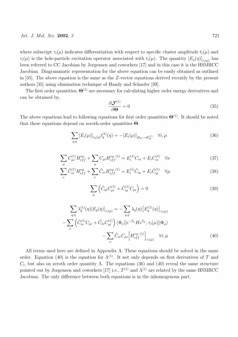
Int. J. Mol. Sci. 2002, 3 721

where subscript τi(µ) indicates differentiation with respect to specific cluster amplitude ti(µ) and

τi(µ) is the hole-particle excitation operator associated with ti(µ). The quantity [Eq(η)]τi(µ) has

been referred to CC Jacobian by Jorgensen and coworkers [17] and in this case it is the HSMRCC

Jacobian. Diagrammatic representation for the above equation can be easily obtained as outlined

in [35]. The above equation is the same as the Z-vector equations derived recently by the present

authors [35] using elimination technique of Handy and Schaefer [39].

The first order quantities, Θ(1) are necessary for calculating higher order energy derivatives and

can be obtained by,∂J (1)

∂Θ= 0 (35)

The above equations lead to following equations for first order quantities Θ(1). It should be noted

that these equations depend on zeroth-order quantities Θ.

∑q,η

[Ei(µ)]τq(η)t(1)q (η) = −[Ei(µ)]

HN→H(1)N

∀i, µ (36)

∑µ

C(1)µi Hνµ

eff +∑

µ

CµiHνµeff

(1) = E(1)i Cνi + EiC

(1)νi ∀ν (37)

∑ν

C(1)iν Hνµ

eff +∑

ν

CiνHνµeff

(1) = E(1)i Ciµ + EiC

(1)iµ ∀µ (38)

∑µ

(CiµC

(1)µi + C

(1)iµ Cµi

)= 0 (39)

∑q,η

λ(1)q (η)[Eq(η)]τi(µ) = −

∑q,η

λq(η)[E(1)

q (η)]τi(µ)

−∑

ν

(C

(1)iν Cµi + CiνC

(1)µi

)〈Φν |[e−TµHeTµ , τi(µ)]|Φµ〉

−∑

ν

CiνCµi

[Hνµ

eff(1)]

τi(µ)∀i, µ (40)

All terms used here are defined in Appendix A. These equations should be solved in the same

order. Equation (40) is the equation for Λ(1). It not only depends on first derivatives of T and

Ci, but also on zeroth order quantity Λ. The equations (36) and (40) reveal the same structure

pointed out by Jorgensen and coworkers [17] i.e., T (1) and Λ(1) are related by the same HSMRCC

Jacobian. The only difference between both equations is in the inhomogenous part.

Int. J. Mol. Sci. 2002, 3 722

3.3 Simplified expressions for Energy derivatives

Energy derivative of n-th order, E(n)i , is just the value of functional J (n), denoted by J (n)

opt , when

the stationary values ofΘ(m) m = 0, n

are substituted in it. Hence, J (n)

opt can be considered as

the required energy derivative and treat Ei as another Lagrange multiplier. It has been shown

that C(n)i and T (n) obey (2n + 1) rule and Lagrange multipliers Λ(n) and E

(n)i obey (2n + 2) rule.

However, the expressions obtained by simple substitution as above do not take advantage of the

above rules. Hence the expressions must be simplified by explicit application of these rules. This

eliminates any unnecessary higher order derivatives present in these expressions. Elimination is

carried out by referring to appropriate response equations, including the zeroth-order response

equations.

ForJ (n)

opt n = 1, 3

the quantities which need to be eliminated are given below, by the appli-

cation of (2n + 1) and (2n + 2) rules.

J (1)opt =⇒

C

(1)i , T (1), E

(1)i , Λ(1)

J (2)

opt =⇒

C(2)i , T (2), E

(2)i , E

(1)i , Λ(2), Λ(1)

J (3)

opt =⇒

C(3)i , C

(2)i , T (3), T (2), E

(3)i , E

(2)i , Λ(3), Λ(2)

In Appendix B, expressions forJ (n)

opt n = 1, 3

obtained from (A-4)-(A-6) are rearranged to

indicate explicit cancellation of higher derivatives of Ci, Λ and Ei. Terms indicated in can

be eliminated by application of response equations of appropriate order. This is discussed in

following subsections. Elimination of higher derivatives of T from the remaining expressions will

be demonstrated seperately.

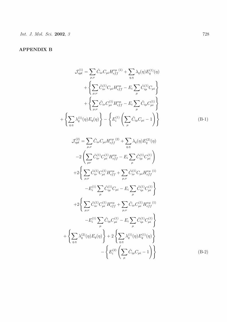
3.3.1 Simplified expression for J (1)opt

Expression for Energy first derivative J (1)opt is given in (B-1). It can be noted that C

(1)µi is

eliminated by zeroth-order equation for Ciν , (21) and C(1)iν is eliminated by zeroth-order equation

for Cµi, (20). The Lagrange multipliers Λ(1) and E(1)i are eliminated by zeroth-order T equation

(19), and biorthogonality equation (23), respectively. Since HSMRCC equations (20)-(21) contain

Ei, presense of Ei is automatically eliminated.

Elimination of T (1) which is present in the surviving terms of (B-1), requires application of

zeroth order Λ equations. For demonstate this, Hνµeff

(1) and E(1)q (η) are expanded to seperate out

terms containing T (1). All such terms cancel precicely from Λ equations, (34). Hence, simplified

Int. J. Mol. Sci. 2002, 3 723

expression for J (1)opt is given by,

J (1)opt =

∑µ,ν

CiνCµi

[Hνµ

eff(1)]

T (0)+∑q,η

λq(η)[E(1)

q (η)]T (0) (41)

where subscript T (n) indicates retention of terms containingT (m) m = 0, n

. This expression has

been further simplified by making use of state-dependent effective CC density matrices [35].

3.3.2 Simplified expression for J (2)opt

Expression for Energy second derivative J (2)opt is given in (B-2) along with grouping necessary

for elimination. Unlike J (1)opt , J (2)

opt depends on T (1) and C(1)i , which are determined by equations

(36)-(39). C(2)i is eliminated by zeroth-order equations for Ci, (20)-(21). Similarly, Λ(2), Λ(1) and

E(2)i are trivially eliminated by T (1) equation (36), T equation (19) and biorhogonality condition

(23) respectively. Although, E(1)i can be easily eliminated from equation (39), we deliberately

retain it to further simplify the expression. Since C(1)i depends on T (1), terms containing both T (1)

and C(1)i can be eliminated using C

(1)i response equations (37)- (38). For this some readjustments

are necessary as indicated in (B-2).

T (2) present in the remaining terms can be eliminated as done in section 3.3.1, by collecting

terms containing T (2), and making use of zeroth-order Λ equations. This leads to simplified

expression for J (2) as

J (2)opt =

∑µ,ν

CiνCµi

[Hνµ

eff(2)]

T (1)+∑q,η

λq(η)[E(2)

q (η)]T (1)

−2

(∑µν

C(1)iν C

(1)µi Hνµ

eff − E∑

µ

C(1)iµ C

(1)µi

)(42)

3.3.3 Simplified expression for J (3)opt

Expression for Energy third derivative J (3)opt is given in (B-3) along with groupings necessary

for elimination. Equation (40) for Λ(1) is the only additional equation to be solved in addition

to T (1) and C(1)i equations. C

(3)i and C

(2)i can be eliminated through Ci and C

(1)i equations

respectively. Similary, Λ(3), Λ(2) , E(3)i , E

(2)i can be trivially eliminated by applying appripriate

response equations.

Presence of T (3) and T (2) can be eliminated by collecting terms containing these quantities

from surviving terms. It can be easily seen that such terms arise with correct factor necessary

for applying Λ and Λ(1) equations. While T (3) cancels from Λ equation (34), cancellation of T (2)

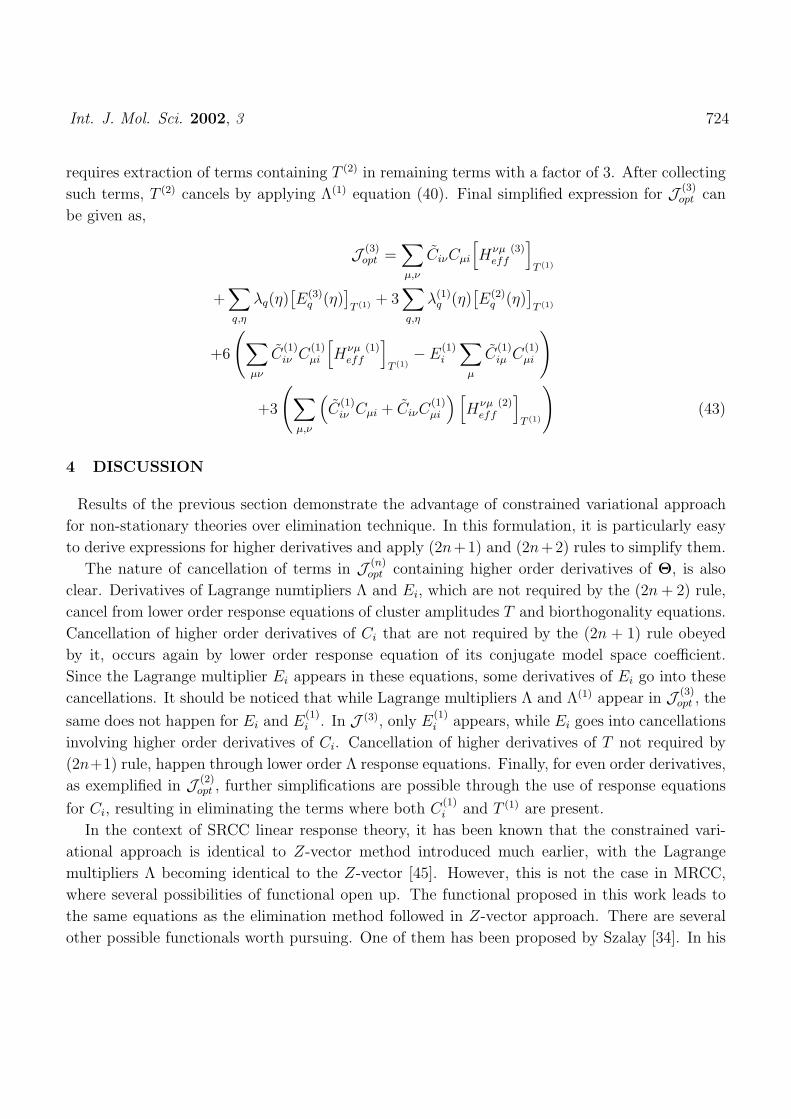
Int. J. Mol. Sci. 2002, 3 724

requires extraction of terms containing T (2) in remaining terms with a factor of 3. After collecting

such terms, T (2) cancels by applying Λ(1) equation (40). Final simplified expression for J (3)opt can

be given as,

J (3)opt =

∑µ,ν

CiνCµi

[Hνµ

eff(3)]

T (1)

+∑q,η

λq(η)[E(3)

q (η)]T (1) + 3

∑q,η

λ(1)q (η)

[E(2)

q (η)]T (1)

+6

(∑µν

C(1)iν C

(1)µi

[Hνµ

eff(1)]

T (1)− E

(1)i

∑µ

C(1)iµ C

(1)µi

)

+3

(∑µ,ν

(C

(1)iν Cµi + CiνC

(1)µi

) [Hνµ

eff(2)]

T (1)

)(43)

4 DISCUSSION

Results of the previous section demonstrate the advantage of constrained variational approach

for non-stationary theories over elimination technique. In this formulation, it is particularly easy

to derive expressions for higher derivatives and apply (2n+1) and (2n+2) rules to simplify them.

The nature of cancellation of terms in J (n)opt containing higher order derivatives of Θ, is also

clear. Derivatives of Lagrange numtipliers Λ and Ei, which are not required by the (2n + 2) rule,

cancel from lower order response equations of cluster amplitudes T and biorthogonality equations.

Cancellation of higher order derivatives of Ci that are not required by the (2n + 1) rule obeyed

by it, occurs again by lower order response equation of its conjugate model space coefficient.

Since the Lagrange multiplier Ei appears in these equations, some derivatives of Ei go into these

cancellations. It should be noticed that while Lagrange multipliers Λ and Λ(1) appear in J (3)opt , the

same does not happen for Ei and E(1)i . In J (3), only E

(1)i appears, while Ei goes into cancellations

involving higher order derivatives of Ci. Cancellation of higher derivatives of T not required by

(2n+1) rule, happen through lower order Λ response equations. Finally, for even order derivatives,

as exemplified in J (2)opt , further simplifications are possible through the use of response equations

for Ci, resulting in eliminating the terms where both C(1)i and T (1) are present.

In the context of SRCC linear response theory, it has been known that the constrained vari-

ational approach is identical to Z-vector method introduced much earlier, with the Lagrange

multipliers Λ becoming identical to the Z-vector [45]. However, this is not the case in MRCC,

where several possibilities of functional open up. The functional proposed in this work leads to

the same equations as the elimination method followed in Z-vector approach. There are several

other possible functionals worth pursuing. One of them has been proposed by Szalay [34]. In his

Int. J. Mol. Sci. 2002, 3 725

functional, a factor of CiµCµi is introduced in the second term of (28). This leads to expressions

for effective CC density matrices which are closer in structure to SRCC counterparts [9]. On the

other hand, such a functional leads to Λ equations whose homogenous part depends on Ci. As

a result, T (n) and Λ(n) do not share the same HSMRCC Jacobian, as it happens in SRCC. On

the other hand, the functional in this work leads to same HSMRCC Jacobian for T (n) and Λ(n).

Although this is a clear advantage, other possibile functionals should be explored. However, it

should be noted that all such functional are equivalent in the sense that they provide same energies

and derivatives differing only in the form of expressions.

Another important aspect of constrained variational approach is the intrinsic state-dependency

of the functional. It should be noted that the state-dependency of Z-vector is not special to MRCC

methods, but it has been observed in Equation of Motion CC method [28, 29]. The present authors

have investigated whether T (1) can be eliminated from Heff(1) in favor of a single Z-vector. It has

been concluded to be not possible for a general case, because of matrix nature of Heff(1). Hence,

it is necessary to become state-selective and eliminate T (1) from the energy deriative of a specific

state.

It has been recognized that constrained variation approach for SRCC is related to bivariational

CC methods investigated by Arponen [13]. The Single-Reference Extended CC (SR-ECC) formu-

lated by Arponen is attractive in many respects and has been investigated for its use in calculating

molecular properties [43–45]. Apart from being stationary, terminating and size-extensive nature

of functional, with all their advantages, it is also known to sum much larger class of perturbation

theory diagrams as compared to SRCC. Hence it is expected to be highly accurate and appro-

priate for use to calculate nonlinear molecular electronic properties. Generalization of SR-ECC

to multi-reference situations (MR-ECC) has not been reported in literature. The nature of con-

strained variation approach for HSMRCC clearly indicates that MR-ECC has to be state-selective

theory, much akin to the decontracted state-selective MRCC approach proposed by Mukherjee

and coworkers [27]. The non-uniqueness of the constrained variational functional indicates that

many different formulations of MR-ECC may be possible. This is similar to the possibilty of

having varieties of state-selective non-stationary MRCC theories. This line of research is worth

pursuing.

5 ACKNOWLEDGEMENTS

The authors acknowledge research grant from the Department of Science and Technology (DST),

India towards the work. One of the authors, KRS, thanks Council of Scientific and Industrial

Research (CSIR), India for research fellowship.

Int. J. Mol. Sci. 2002, 3 726

APPENDIX A

Expressions for functionals J (n) in (30) can be obtained by expanding various quantities on

the right hand side of (28) as a Taylor series in perturbation strength in g. In the following,

superscript on zeroth-order quantities are dropped.

Eq(η, g) = Eq(η) + gE(1)q (η) +

1

2!g2E(2)

q (η) + · · · (A-1)

Hνµeff (g) = Hνµ

eff + gHνµeff

(1) +1

2!g2Hνµ

eff(2) + · · · (A-2)

Θ(g) = Θ + gΘ(1) +1

2!g2Θ(2) + · · · (A-3)

Collecting and equating terms of same order in g on both sides after the expansion, we get,

J (1) =∑µ,ν

(C

(1)iν Cµi + CiνC

(1)µi

)Hνµ

eff +∑µ,ν

CiνCµiHνµeff

(1) +

∑q,η

λ(1)q (η)Eq(η) +

∑q,η

λq(η)E(1)q (η)

−E(1)i

(∑µ

CiµCµi − 1

)− Ei

(∑µ

(C

(1)iµ Cµi + CiµC

(1)µi

))(A-4)

J (2) =∑µ,ν

(C

(2)iν Cµi + CiνC

(2)µi

)Hνµ

eff +∑µ,ν

CiνCµiHνµeff

(2) +

2∑µ,ν

C(1)iν C

(1)µi Hνµ

eff + 2∑µ,ν

(C

(1)iν Cµi + CiνC

(1)µi

)Hνµ

eff(1)

+∑q,η

λ(2)q (η)Eq(η) +

∑q,η

λq(η)E(2)q (η) + 2

∑q,η

λ(1)q (η)E(1)

q (η)

−E(2)i

(∑µ

CiµCµi − 1

)− Ei

(∑µ

(C

(2)iµ Cµi + CiµC

(2)µi

))

−2Ei

(∑µ

C(1)iµ C

(1)µi

)− 2E

(1)i

(∑µ

(C

(1)iµ Cµi + CiµC

(1)µi

))(A-5)

Int. J. Mol. Sci. 2002, 3 727

J (3) =∑µ,ν

(C

(3)iν Cµi + CiνC

(3)µi

)Hνµ

eff +∑µ,ν

CiνCµiHνµeff

(3)

+3∑µ,ν

(C

(2)iν C

(1)µi + C

(1)iν C

(2)µi

)Hνµ

eff

+3∑µ,ν

(C

(2)iν Cµi + CiνC

(2)µi

)Hνµ

eff(1)

+3∑µ,ν

(C

(1)iν Cµi + CiνC

(1)µi

)Hνµ

eff(2)

+6∑µ,ν

C(1)iν C

(1)µi Hνµ

eff(1)

+∑q,η

λ(3)q (η)Eq(η)

∑q,η

λq(η)E(3)q (η)

+3∑q,η

λ(2)q (η)E(1)

q (η) + 3∑q,η

λ(1)q (η)E(2)

q (η)

−E(3)i

(∑µ

CiµCµi − 1

)− Ei

(∑µ

(C

(3)iµ Cµi + CiµC

(3)µi

))

−3E(2)i

(∑µ

(C

(1)iµ Cµi + CiµC

(1)µi

))

−3E(1)i

(∑µ

(C

(2)iµ Cµi + CiµC

(2)µi

))

−3Ei

(∑µ

(C

(2)iµ C

(1)µi + C

(1)iµ C

(2)µi

))

−6E(1)i

∑µ

C(1)iµ C

(1)µi (A-6)

Int. J. Mol. Sci. 2002, 3 728

APPENDIX B

J (1)opt =

∑µ,ν

CiνCµiHνµeff

(1) +∑q,η

λq(η)E(1)q (η)

+

∑µ,ν

C(1)iν CµiH

νµeff − Ei

∑µ

C(1)iµ Cµi

+

∑µ,ν

CiνC(1)µi Hνµ

eff − Ei

∑µ

CiµC(1)µi

+

∑q,η

λ(1)q (η)Eq(η)

−

E(1)i

(∑µ

CiµCµi − 1

)(B-1)

J (2)opt =

∑µ,ν

CiνCµiHνµeff

(2) +∑q,η

λq(η)E(2)q (η)

−2

(∑µν

C(1)iν C

(1)µi Hνµ

eff − Ei

∑µ

C(1)iµ C

(1)µi

)

+2

∑µ,ν

C(1)iν C

(1)µi Hνµ

eff +∑µ,ν

C(1)iν CµiH

νµeff

(1)

−E(1)i

∑µ

C(1)iµ Cµi − Ei

∑µ

C(1)iµ C

(1)µi

+2

∑µ,ν

C(1)iν C

(1)µi Hνµ

eff +∑µ,ν

CiνC(1)µi Hνµ

eff(1)

−E(1)i

∑µ

CiµC(1)µi − Ei

∑µ

C(1)iµ C

(1)µi

+

∑q,η

λ(2)q (η)Eq(η)

+ 2

∑q,η

λ(1)q (η)E(1)

q (η)

−

E(2)i

(∑µ

CiµCµi − 1

)(B-2)

Int. J. Mol. Sci. 2002, 3 729

J (3)opt =

∑µ,ν

CiνCµiHνµeff

(3) +∑q,η

λq(η)E(3)q (η) + 3

∑q,η

λ(1)q (η)E(2)

q (η)

+6

(∑µν

C(1)iν C

(1)µi Hνµ

eff(1) − E

(1)i

∑µ

C(1)iµ C

(1)µi

)

+3

(∑µ,ν

(C

(1)iν Cµi + CiνC

(1)µi

)Hνµ

eff(2)

)

+

∑µ,ν

C(3)iν CµiH

νµeff − Ei

∑µ

C(3)iµ Cµi

+

∑µ,ν

CiνC(3)µi Hνµ

eff − Ei

∑µ

CiµC(3)µi

+3

∑µ,ν

C(2)iν C

(1)µi Hνµ

eff +∑µ,ν

C(2)iν CµiH

νµeff

(1)

−E(1)i

∑µ

C(2)iµ Cµi − Ei

∑µ

C(2)iµ C

(1)µi

+3

∑µ,ν

C(1)iν C

(2)µi Hνµ

eff +∑µ,ν

CiνC(2)µi Hνµ

eff(1)

−E(1)i

∑µ

CiµC(2)µi − Ei

∑µ

C(1)iµ C

(2)µi

+

∑q,η

λ(3)q (η)Eq(η)

+ 3

∑q,η

λ(2)q (η)E(1)

q (η)

−

E(2)i

(∑µ

CiµCµi − 1

)−

3E(2)i

(∑µ

(C

(1)iµ Cµi + CiµC

(1)µi

))(B-3)

References

1. Cizek, J. Adv. Quant. Chem. 1969, 14, 35

2. Bartlett, R.J. Annu. Rev. Phys. Chem. 1981, 32, 359

3. Paldus, J. in Methods in Computational Molecular Physics ; Wilson, S.; Dierckson, G.H.F.

Ed. NATO ASI series B, Plenum, NY, 1992.

4. Helgaker, T.; Jorgensen, P. Adv. Quant. Chem. 1988, 19, 183

Int. J. Mol. Sci. 2002, 3 730

5. Bartlett, R.J. in Geometrical Derivatives of Energy Surface and Molecular properties; Jor-

gensen, P.; Simons, J. Ed. Reidel, Dordrecht, 1986

6. Oslen, J.; Jorgensen, P. in Modern Electronic Structure Theory, Part II ; Yarkony, D.R. Ed.

World Scientific, Singapore, 1995

7. Epstein, S.T. in The Variation Principle in Quantum Chemistry ; Academic, NY, 1974

8. Adamowicz, L.; Laidig, W.D.; Bartlett, R.J. Int. J. Quant. Chem. Symp. 1984, 18, 245

9. Fitzgerald, G.; Harrison, R.J.; Bartlett, R.J. J. Chem. Phys. 1986, 85, 5143

10. (a) Salter, E.A.; Trucks, G.W.; Bartlett, R.J. J. Chem. Phys 1989, 90, 1752; (b) Salter,

E.A.; Bartlett, R.J. J. Chem. Phys 1989, 90, 1767

11. (a) Bartlett, R.J.; Noga, J. Chem. Phys. Lett. 1988, 150, 29; (b) Bartlett, R.J.; Kucharski,

S.A.; Noga, J. Chem. Phys. Lett. 1989, 155, 133

12. Pal, S.; Ghose, K.B. Curr. Science 1992, 63, 667

13. Arponen, J. Ann. Phys, 1983, 151, 311

14. (a) Voorhis, T.V.; Head-Gordon, M. Chem. Phys. Lett. 2000, 330, 585 (b) Voorhis, T.V.;

Head-Gordon, M. J. Chem. Phys. 2000, 113, 8873

15. Jorgensen, P.; Helgaker, T. J. Chem. Phys. 1988, 89, 1560

16. Helgaker, T.; Jorgensen, P. Theor. Chim. Acta. 1989, 75, 111

17. Koch, H; Jensen, H.J.A.; Jorgensen, P.; Helgaker, T.; Scuseria, G.E.; Schaefer III, H.F. J.

Chem. Phys 1990, 92, 4924

18. Koch, H.; Jorgensen, P. J. Chem. Phys. 1990, 93, 3333

19. Mukherjee, D.; Lindgren, I. Phys. Rep. 1987, 151, 93

20. Mukherjee, D.; Pal, S. Adv. Quant. Chem. 1989, 20, 291

21. Durand, P.; Malrieu, J.P. Adv. Chem. Phys 1987, 67, 321

22. Hurtubise, V.; Freed, K.F. Adv. Chem. Phys 1993, 83, 465

23. Jezioroski, B.; Monkhorst, H.J.M. Phys. Rev. A., 1982, 24, 1668

Int. J. Mol. Sci. 2002, 3 731

24. (a) Meissner, L.; Kucharski, S.A.; Bartlett, R.J. J. Chem. Phys, 1989, 91, 6187 (b) Meissner,

L.; Bartlett, R.J. J. Chem. Phys, 1990, 92, 561

25. Mukhopadhyay, D.; Datta, B.; Mukherjee, D. Chem. Phys. Lett. 1992, 197, 236

26. Mahapatra, U.S.; Datta, B.; Mukherjee, D. in Recent Advances in Coupled-Cluster Methods ;

Bartlett, R.J. Ed. World Scientific, Singapore, 1997

27. Mahapatra, U.S.; Datta, B.; Bandopadhyay, B.; Mukherjee, D. Adv. Quant. Chem 1998,

30, 163

28. Stanton, J.F. J. Chem. Phys. 1993, 99, 8840

29. (a) Stanton, J.F.; Gauss, J. J. Chem. Phys. 1994, 100, 4695; (b) Stanton, J.F.; Gauss, J;

Theo. Chim. Acta. 1995, 91, 267; (c) Stanton, J.F.; Gauss, J. J. Chem. Phys. 1994, 101,

8938

30. This point is in clarification to the comments of one of the reviewers.

31. Pal, S. Phys. Rev. A. 1989, 39, 39

32. Pal, S. Int. J. Quant. Chem. 1992, 41, 443

33. (a) Ajitha, D.; Vaval, N.; Pal, S. J. Chem. Phys. 1999, 110, 2316; (b) Ajitha, D.; Pal, S.

Chem. Phys. Lett. 1999, 309, 457; (c) Ajitha, D.; Pal, S. J. Chem. Phys. 2001, 114, 3380

34. Szalay, P. Int. J. Quant. Chem. 1994, 55, 152

35. Shamasundar, K.R.; Pal, S. J. Chem. Phys., 2001, 114, 1981; ibid. 2001, 115, 1979(E)

36. Monkhorst, H.J. Int. J. Quant. Chem. Symp. 1977, 11, 421

37. Jorgensen, P.; Simons, J. J. Chem. Phys. 1983, 79,334

38. Dalgarno, A.; Stewart, A.L. Proc. Roy. Soc. Lon. Ser A 238, 269

39. Handy, N.C.; Schaefer III, H.F. J. Chem. Phys. 1984, 81, 5031

40. Rice, J.E.; Amos, R.D. Chem. Phys. Lett. 1985, 122, 585

41. Fitzgerald, G.; Harrison, R.J.; Bartlett, R.J. Chem. Phys. Lett. 1985, 117, 433

42. Scheiner, A.C.; Scuseria, G.E.; Lee, T.J.; Schaefer III, H.F. J. Chem. Phys 1987, 87, 5361

Int. J. Mol. Sci. 2002, 3 732

43. (a) Vaval, N.; Ghose, K.B.; Pal, S. J. Chem. Phys. 1994, 101, 4914

44. (a) Kumar, A.B.; Vaval, N.; Pal, S. Chem. Phys. Lett. 1998, 295, 189; (b) Vaval, N.; Kumar,

A.B.; Pal, S. Int. J. Mol. Sci. 2001, 2, 89

45. Vaval, N.; Pal, S. Phys. Rev. A. 1996, 54, 250

46. (a) Haque, M.; Kaldor, U. Chem. Phys. Lett. 1985, 117, 347; (b) ibid. 1985, 120, 261; (c)

Hughes, S.R.; Kaldor, U. Phys. Rev. A. 1993, 47, 4705

47. (a) Pal, S.; Rittby, M.; Bartlett, R.J.; Sinha, D.; Mukherjee, D. J. Chem. Phys. 1988, 88,

4357; (b) ibid. Chem. Phys. Lett. 1987, 137, 273; (c) Vaval, N.; Pal, S.; Mukherjee, D.

Theor. Chim. Acc. 1998, 99, 100; (d) Vaval, N.; Pal, S. J. Chem. Phys. 1999, 111, 4051

48. (a) Meissner, L.; Jankowski, K.; Wasilewski,J. Int. J. Quant. Chem 1988, 34, 535; (b)

Balkova, A.; Kucharski, S.A.; Meissner, L.; Bartlett, R.J. Theor. Chim. Acta 1991, 80,

335; (c) ibid. J. Chem. Phys. 1991, 95, 4311; (d) Balkova, A.; Kucharski, S.A.; Bartlett,

R.J. Chem. Phys. Lett 1991, 182, 511; (e) Kucharski, S.A.; Bartlett, R.J. J. Chem. Phys

1989, 95, 8227; (f) Balkova, A.; Bartlett, R.J. Chem. Phys. Lett. 1992, 193, 364

49. (a) Paldus, J.; Piecuch, P.; Jeziorski, B.; Pylypow, L. in Recent Progress in Many-Body

Theories, Vol.3 ; Ainsworthy, T.L.; Campbell, C.E.; Clements, B.E.; Krotschek, E. Ed.

Plenum Press, New York, 1992; (b) Paldus, J.; Piecuch, P.; Pylypow, L.; Jeziorski, B.

Phys. Rev. A. 1993, 47, 2738; (c) Piecuch, P.; Tobola, R.; Paldus, J. Chem. Phys. Lett.

1993, 210, 243; (d) Piecuch, P.; Paldus, J. Phys. Rev. A. 1994, 49, 3479; (e) Kowalski, K.;

Piecuch, P. Phys. Rev. A. 2000, 61, page number

50. (a) Berkovic, S.; Kaldor, U. Chem. Phys. Lett. 1992, 199, 42; (b) ibid. J. Chem. Phys.

1993, 98, 3090

51. (a) Jezioroski, B.; Paldus, J. J. Chem. Phys 1988, 88, 5673; (b) Piecuch, P.; Paldus, J.

Theor. Chim. Acta. 1992, 83, 69; (c) Piecuch, P.; Paldus, J. J. Chem. Phys. 1994, 101,

5875; (d) Piecuch, P.; Paldus, J. J. Phys. Chem. 1995, 99, 15354

52. Ajitha, D.; Pal, S. Phys. Rev. A. 1997, 56, 2658

53. Ajitha, D.; Pal, S. J. Chem. Phys. 1999, 111, 3832; ibid. 1999, 111, 9892(E)

54. Pal, S. Theor. Chim. Acta. 1984, 66, 151