PARTIAL DERIVATIVES - E-Library
119
OVERVIEW In studying a real-world phenomenon, a quantity being investigated usually depends on two or more independent variables. So we need to extend the basic ideas of the calculus of functions of a single variable to functions of several variables. Although the calculus rules remain essentially the same, the calculus is even richer. The derivatives of functions of several variables are more varied and more interesting because of the different ways in which the variables can interact. Their integrals lead to a greater variety of appli- cations. The studies of probability, statistics, fluid dynamics, and electricity, to mention only a few, all lead in natural ways to functions of more than one variable. 965 P ARTIAL DERIVATIVES Chapter 14 Functions of Several Variables Many functions depend on more than one independent variable. The function calculates the volume of a right circular cylinder from its radius and height. The function calculates the height of the paraboloid above the point P(x, y) from the two coordinates of P. The temperature T of a point on Earth’s surface depends on its latitude x and longitude y, expressed by writing In this sec- tion, we define functions of more than one independent variable and discuss ways to graph them. Real-valued functions of several independent real variables are defined much the way you would imagine from the single-variable case. The domains are sets of ordered pairs (triples, quadruples, n-tuples) of real numbers, and the ranges are sets of real numbers of the kind we have worked with all along. T = ƒs x, y d. z = x 2 + y 2 ƒs x, y d = x 2 + y 2 V = pr 2 h 14.1 DEFINITIONS Function of n Independent Variables Suppose D is a set of n-tuples of real numbers A real-valued function ƒ on D is a rule that assigns a unique (single) real number to each element in D. The set D is the function’s domain. The set of w-values taken on by ƒ is the function’s range. The symbol w is the dependent variable of ƒ, and ƒ is said to be a function of the n independent variables to We also call the ’s the function’s input variables and call w the function’s output variable. x j x n . x 1 w = ƒs x 1 , x 2 , Á , x n d s x 1 , x 2 , Á , x n d.
-
Upload
khangminh22 -
Category
Documents
-
view
0 -
download
0
Transcript of PARTIAL DERIVATIVES - E-Library
OVERVIEW In studying a real-world phenomenon, a quantity being investigated usuallydepends on two or more independent variables. So we need to extend the basic ideas of thecalculus of functions of a single variable to functions of several variables. Although thecalculus rules remain essentially the same, the calculus is even richer. The derivatives offunctions of several variables are more varied and more interesting because of the differentways in which the variables can interact. Their integrals lead to a greater variety of appli-cations. The studies of probability, statistics, fluid dynamics, and electricity, to mentiononly a few, all lead in natural ways to functions of more than one variable.
965
PARTIAL DERIVATIVES
C h a p t e r
14
Functions of Several Variables
Many functions depend on more than one independent variable. The function calculates the volume of a right circular cylinder from its radius and height. The function
calculates the height of the paraboloid above the pointP(x, y) from the two coordinates of P. The temperature T of a point on Earth’s surfacedepends on its latitude x and longitude y, expressed by writing In this sec-tion, we define functions of more than one independent variable and discuss ways tograph them.
Real-valued functions of several independent real variables are defined much the wayyou would imagine from the single-variable case. The domains are sets of ordered pairs(triples, quadruples, n-tuples) of real numbers, and the ranges are sets of real numbers ofthe kind we have worked with all along.
T = ƒsx, yd.
z = x 2+ y 2ƒsx, yd = x 2
+ y 2
V = pr 2h
14.1
DEFINITIONS Function of n Independent VariablesSuppose D is a set of n-tuples of real numbers A real-valuedfunction ƒ on D is a rule that assigns a unique (single) real number
to each element in D. The set D is the function’s domain. The set of w-valuestaken on by ƒ is the function’s range. The symbol w is the dependent variableof ƒ, and ƒ is said to be a function of the n independent variables to Wealso call the ’s the function’s input variables and call w the function’s outputvariable.
xj
xn.x1
w = ƒsx1, x2, Á , xnd
sx1, x2, Á , xnd.
4100 AWL/Thomas_ch14p965-1066 8/25/04 2:52 PM Page 965
If ƒ is a function of two independent variables, we usually call the independent vari-ables x and y and picture the domain of ƒ as a region in the xy-plane. If ƒ is a function ofthree independent variables, we call the variables x, y, and z and picture the domain as aregion in space.
In applications, we tend to use letters that remind us of what the variables stand for. Tosay that the volume of a right circular cylinder is a function of its radius and height, wemight write To be more specific, we might replace the notation ƒ(r, h) by theformula that calculates the value of V from the values of r and h, and write Ineither case, r and h would be the independent variables and V the dependent variable ofthe function.
As usual, we evaluate functions defined by formulas by substituting the values of the in-dependent variables in the formula and calculating the corresponding value of the dependentvariable.
EXAMPLE 1 Evaluating a Function
The value of at the point (3, 0, 4) is
From Section 12.1, we recognize ƒ as the distance function from the origin to the point(x, y, z) in Cartesian space coordinates.
Domains and Ranges
In defining a function of more than one variable, we follow the usual practice of excludinginputs that lead to complex numbers or division by zero. If cannotbe less than If cannot be zero. The domain of a function is as-sumed to be the largest set for which the defining rule generates real numbers, unless thedomain is otherwise specified explicitly. The range consists of the set of output values forthe dependent variable.
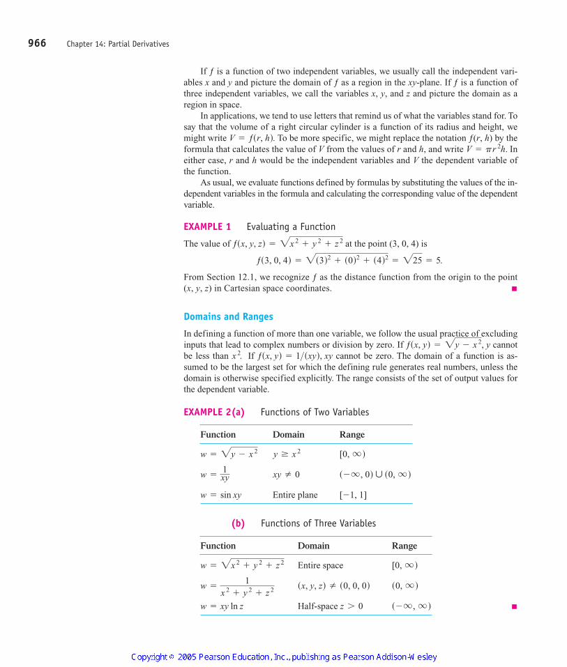
EXAMPLE 2(a) Functions of Two Variables
Function Domain Range
Entire plane
(b) Functions of Three Variables
Function Domain Range
Entire space
Half-space s - q , q dz 7 0w = xy ln z
s0, q dsx, y, zd Z s0, 0, 0dw =1
x 2+ y 2
+ z 2
[0, q dw = 2x 2+ y 2
+ z 2
[-1, 1]w = sin xy
s - q , 0d ´ s0, q dxy Z 0w =1xy
[0, q dy Ú x 2w = 2y - x 2
ƒsx, yd = 1>sxyd, xyx 2.ƒsx, yd = 2y - x 2, y
ƒs3, 0, 4d = 2s3d2+ s0d2
+ s4d2= 225 = 5.
ƒsx, y, zd = 2x 2+ y 2
+ z 2
V = pr 2h.V = ƒsr, hd.
966 Chapter 14: Partial Derivatives
4100 AWL/Thomas_ch14p965-1066 8/25/04 2:52 PM Page 966
Functions of Two Variables
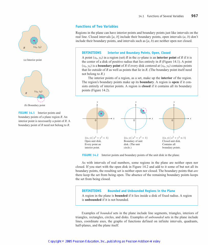
Regions in the plane can have interior points and boundary points just like intervals on thereal line. Closed intervals [a, b] include their boundary points, open intervals (a, b) don’tinclude their boundary points, and intervals such as [a, b) are neither open nor closed.
14.1 Functions of Several Variables 967
R
(a) Interior point
R
(b) Boundary point
(x0, y0)
(x0, y0)
FIGURE 14.1 Interior points andboundary points of a plane region R. Aninterior point is necessarily a point of R. Aboundary point of R need not belong to R.
DEFINITIONS Interior and Boundary Points, Open, ClosedA point in a region (set) R in the xy-plane is an interior point of R if it isthe center of a disk of positive radius that lies entirely in R (Figure 14.1). A point
is a boundary point of R if every disk centered at contains pointsthat lie outside of R as well as points that lie in R. (The boundary point itself neednot belong to R.)
The interior points of a region, as a set, make up the interior of the region.The region’s boundary points make up its boundary. A region is open if it con-sists entirely of interior points. A region is closed if it contains all its boundarypoints (Figure 14.2).
sx0, y0dsx0, y0d
sx0, y0d
y
x0
y
x0
y
x0
{(x, y) � x2 � y2 � 1}Open unit disk.Every point aninterior point.
{(x, y) � x2 � y2 � 1}Boundary of unitdisk. (The unitcircle.)
{(x, y) � x2 � y2 � 1}Closed unit disk.Contains allboundary points.
FIGURE 14.2 Interior points and boundary points of the unit disk in the plane.
DEFINITIONS Bounded and Unbounded Regions in the PlaneA region in the plane is bounded if it lies inside a disk of fixed radius. A regionis unbounded if it is not bounded.
As with intervals of real numbers, some regions in the plane are neither open norclosed. If you start with the open disk in Figure 14.2 and add to it some of but not all itsboundary points, the resulting set is neither open nor closed. The boundary points that arethere keep the set from being open. The absence of the remaining boundary points keepsthe set from being closed.
Examples of bounded sets in the plane include line segments, triangles, interiors oftriangles, rectangles, circles, and disks. Examples of unbounded sets in the plane includelines, coordinate axes, the graphs of functions defined on infinite intervals, quadrants,half-planes, and the plane itself.
4100 AWL/Thomas_ch14p965-1066 8/25/04 2:52 PM Page 967
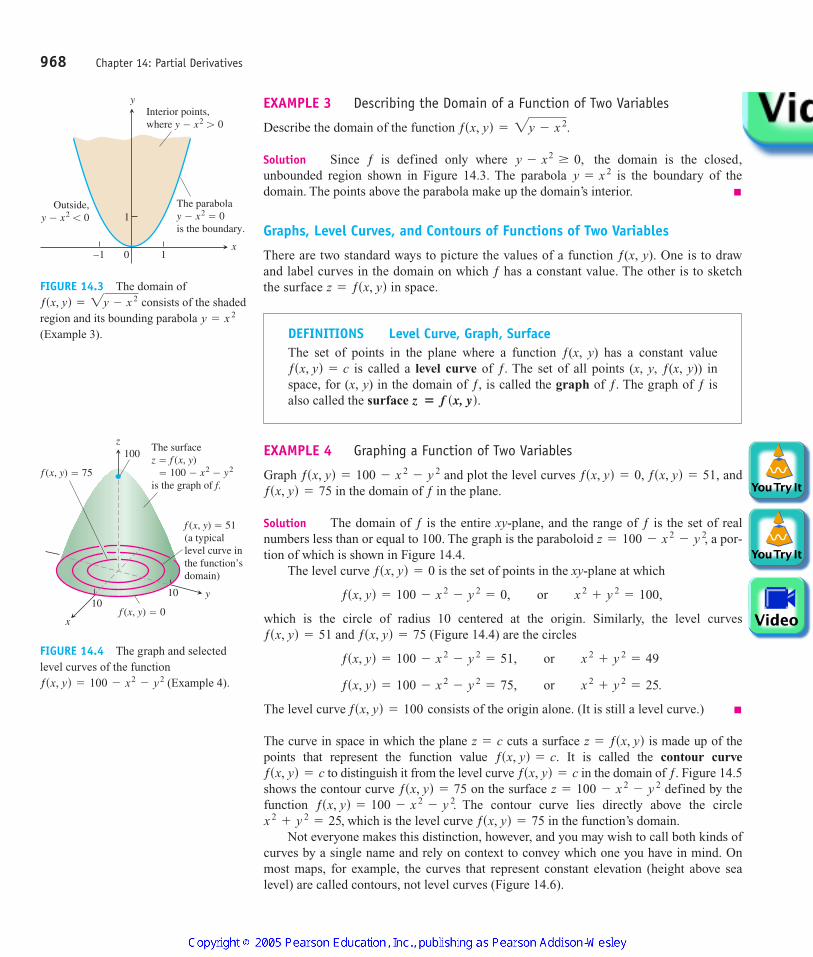
EXAMPLE 3 Describing the Domain of a Function of Two Variables
Describe the domain of the function
Solution Since ƒ is defined only where the domain is the closed,unbounded region shown in Figure 14.3. The parabola is the boundary of thedomain. The points above the parabola make up the domain’s interior.
Graphs, Level Curves, and Contours of Functions of Two Variables
There are two standard ways to picture the values of a function ƒ(x, y). One is to drawand label curves in the domain on which ƒ has a constant value. The other is to sketchthe surface in space.z = ƒsx, yd
y = x 2y - x2
Ú 0,
ƒsx, yd = 2y - x 2.
968 Chapter 14: Partial Derivatives
y
x0 1–1
1
Interior points,where y � x2 � 0
The parabolay � x2 � 0is the boundary.
Outside,y � x2 � 0
FIGURE 14.3 The domain ofconsists of the shaded
region and its bounding parabola (Example 3).
y = x 2ƒsx, yd = 2y - x 2
EXAMPLE 4 Graphing a Function of Two Variables
Graph and plot the level curves andin the domain of ƒ in the plane.
Solution The domain of ƒ is the entire xy-plane, and the range of ƒ is the set of realnumbers less than or equal to 100. The graph is the paraboloid a por-tion of which is shown in Figure 14.4.
The level curve is the set of points in the xy-plane at which
which is the circle of radius 10 centered at the origin. Similarly, the level curvesand (Figure 14.4) are the circles
The level curve consists of the origin alone. (It is still a level curve.)
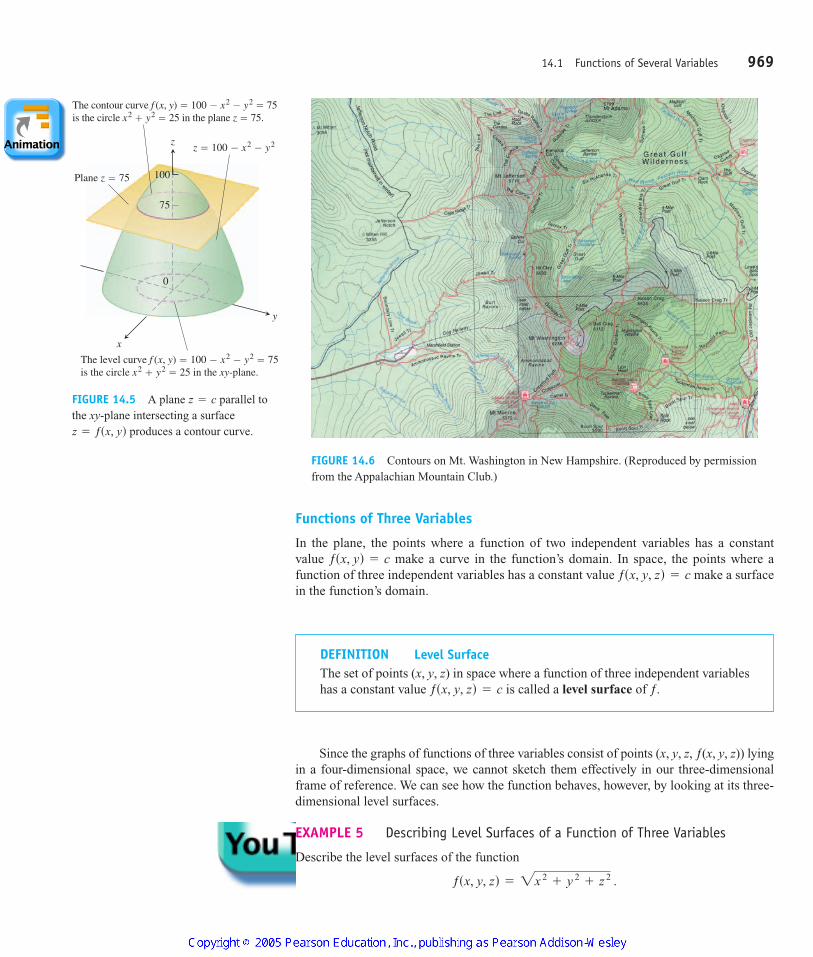
The curve in space in which the plane cuts a surface is made up of thepoints that represent the function value It is called the contour curve
to distinguish it from the level curve in the domain of ƒ. Figure 14.5shows the contour curve on the surface defined by thefunction The contour curve lies directly above the circle
which is the level curve in the function’s domain.Not everyone makes this distinction, however, and you may wish to call both kinds of
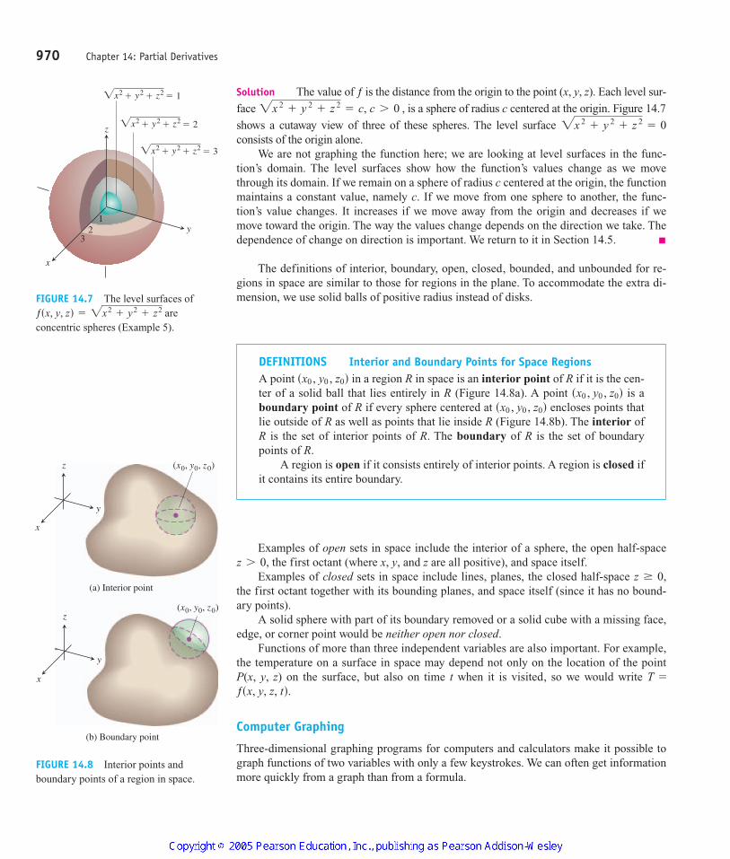
curves by a single name and rely on context to convey which one you have in mind. Onmost maps, for example, the curves that represent constant elevation (height above sealevel) are called contours, not level curves (Figure 14.6).
ƒsx, yd = 75x 2+ y 2
= 25,ƒsx, yd = 100 - x 2
- y 2.z = 100 - x 2
- y 2ƒsx, yd = 75ƒsx, yd = cƒsx, yd = c
ƒsx, yd = c.z = ƒsx, ydz = c
ƒsx, yd = 100
ƒsx, yd = 100 - x 2- y 2
= 75, or x 2+ y 2
= 25.
ƒsx, yd = 100 - x 2- y 2
= 51, or x 2+ y 2
= 49
ƒsx, yd = 75ƒsx, yd = 51
ƒsx, yd = 100 - x 2- y 2
= 0, or x 2+ y 2
= 100,
ƒsx, yd = 0
z = 100 - x 2- y 2,
ƒsx, yd = 75ƒsx, yd = 0, ƒsx, yd = 51,ƒsx, yd = 100 - x 2
- y 2
y
z
x
1010
100
f (x, y) � 75
f (x, y) � 0
f (x, y) � 51(a typicallevel curve inthe function’sdomain)
The surfacez � f (x, y) � 100 � x2 � y2
is the graph of f.
FIGURE 14.4 The graph and selectedlevel curves of the function
(Example 4).ƒsx, yd = 100 - x2- y2
DEFINITIONS Level Curve, Graph, SurfaceThe set of points in the plane where a function ƒ(x, y) has a constant value
is called a level curve of ƒ. The set of all points (x, y, ƒ(x, y)) inspace, for (x, y) in the domain of ƒ, is called the graph of ƒ. The graph of ƒ isalso called the surface z � f sx, yd.
ƒsx, yd = c
4100 AWL/Thomas_ch14p965-1066 8/25/04 2:52 PM Page 968
14.1 Functions of Several Variables 969
z
x
0
y
75
100
The contour curve f (x, y) � 100 � x2 � y2 � 75is the circle x2 � y2 � 25 in the plane z � 75.
Plane z � 75
The level curve f (x, y) � 100 � x2 � y2 � 75is the circle x2 � y2 � 25 in the xy-plane.
z � 100 � x2 � y2
FIGURE 14.5 A plane parallel tothe xy-plane intersecting a surface
produces a contour curve.z = ƒsx, yd
z = c
DEFINITION Level SurfaceThe set of points (x, y, z) in space where a function of three independent variableshas a constant value is called a level surface of ƒ.ƒsx, y, zd = c
FIGURE 14.6 Contours on Mt. Washington in New Hampshire. (Reproduced by permissionfrom the Appalachian Mountain Club.)
Functions of Three Variables
In the plane, the points where a function of two independent variables has a constantvalue make a curve in the function’s domain. In space, the points where afunction of three independent variables has a constant value make a surfacein the function’s domain.
ƒsx, y, zd = cƒsx, yd = c
Since the graphs of functions of three variables consist of points (x, y, z, ƒ(x, y, z)) lyingin a four-dimensional space, we cannot sketch them effectively in our three-dimensionalframe of reference. We can see how the function behaves, however, by looking at its three-dimensional level surfaces.
EXAMPLE 5 Describing Level Surfaces of a Function of Three Variables
Describe the level surfaces of the function
ƒsx, y, zd = 2x 2+ y 2
+ z 2 .
4100 AWL/Thomas_ch14p965-1066 9/2/04 11:09 AM Page 969
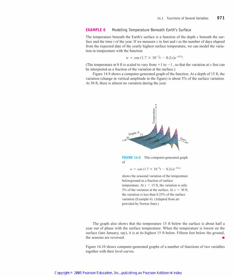
Solution The value of ƒ is the distance from the origin to the point (x, y, z). Each level sur-
face is a sphere of radius c centered at the origin. Figure 14.7
shows a cutaway view of three of these spheres. The level surface consists of the origin alone.
We are not graphing the function here; we are looking at level surfaces in the func-tion’s domain. The level surfaces show how the function’s values change as we movethrough its domain. If we remain on a sphere of radius c centered at the origin, the functionmaintains a constant value, namely c. If we move from one sphere to another, the func-tion’s value changes. It increases if we move away from the origin and decreases if wemove toward the origin. The way the values change depends on the direction we take. Thedependence of change on direction is important. We return to it in Section 14.5.
The definitions of interior, boundary, open, closed, bounded, and unbounded for re-gions in space are similar to those for regions in the plane. To accommodate the extra di-mension, we use solid balls of positive radius instead of disks.
2x 2+ y 2
+ z 2= 0
2x 2+ y 2
+ z 2= c, c 7 0 ,
970 Chapter 14: Partial Derivatives
DEFINITIONS Interior and Boundary Points for Space RegionsA point in a region R in space is an interior point of R if it is the cen-ter of a solid ball that lies entirely in R (Figure 14.8a). A point is aboundary point of R if every sphere centered at encloses points thatlie outside of R as well as points that lie inside R (Figure 14.8b). The interior ofR is the set of interior points of R. The boundary of R is the set of boundarypoints of R.
A region is open if it consists entirely of interior points. A region is closed ifit contains its entire boundary.
sx0 , y0 , z0dsx0 , y0 , z0d
sx0 , y0 , z0d
x
y
z
(a) Interior point
x
y
z
(b) Boundary point
(x0, y0, z0)
(x0, y0, z0)
FIGURE 14.8 Interior points andboundary points of a region in space.
Examples of open sets in space include the interior of a sphere, the open half-spacethe first octant (where x, y, and z are all positive), and space itself.
Examples of closed sets in space include lines, planes, the closed half-space the first octant together with its bounding planes, and space itself (since it has no bound-ary points).
A solid sphere with part of its boundary removed or a solid cube with a missing face,edge, or corner point would be neither open nor closed.
Functions of more than three independent variables are also important. For example,the temperature on a surface in space may depend not only on the location of the pointP(x, y, z) on the surface, but also on time t when it is visited, so we would write
Computer Graphing
Three-dimensional graphing programs for computers and calculators make it possible tograph functions of two variables with only a few keystrokes. We can often get informationmore quickly from a graph than from a formula.
ƒsx, y, z, td.T =
z Ú 0,z 7 0,
x
y
z
12
3
�x2 � y2 � z2 � 3
�x2 � y2 � z2 � 2
�x2 � y2 � z2 � 1
FIGURE 14.7 The level surfaces ofare
concentric spheres (Example 5).ƒsx, y, zd = 2x2
+ y2+ z2
4100 AWL/Thomas_ch14p965-1066 9/2/04 11:09 AM Page 970
EXAMPLE 6 Modeling Temperature Beneath Earth’s Surface
The temperature beneath the Earth’s surface is a function of the depth x beneath the sur-face and the time t of the year. If we measure x in feet and t as the number of days elapsedfrom the expected date of the yearly highest surface temperature, we can model the varia-tion in temperature with the function
(The temperature at 0 ft is scaled to vary from to so that the variation at x feet canbe interpreted as a fraction of the variation at the surface.)
Figure 14.9 shows a computer-generated graph of the function. At a depth of 15 ft, thevariation (change in vertical amplitude in the figure) is about 5% of the surface variation.At 30 ft, there is almost no variation during the year.
-1 ,+1
w = cos s1.7 * 10-2t - 0.2xde-0.2x.
14.1 Functions of Several Variables 971
Days
1530
tx
w
Depth, ft
Tem
pera
ture
FIGURE 14.9 This computer-generated graphof
shows the seasonal variation of the temperaturebelowground as a fraction of surfacetemperature. At the variation is only5% of the variation at the surface. At the variation is less than 0.25% of the surfacevariation (Example 6). (Adapted from artprovided by Norton Starr.)
x = 30 ft,x = 15 ft,
w = cos s1.7 * 10-2t - 0.2xde-0.2x
The graph also shows that the temperature 15 ft below the surface is about half ayear out of phase with the surface temperature. When the temperature is lowest on thesurface (late January, say), it is at its highest 15 ft below. Fifteen feet below the ground,the seasons are reversed.
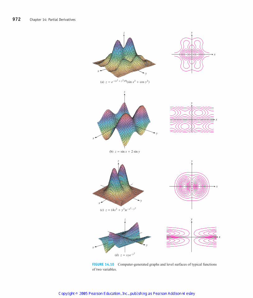
Figure 14.10 shows computer-generated graphs of a number of functions of two variablestogether with their level curves.
4100 AWL/Thomas_ch14p965-1066 8/25/04 2:52 PM Page 971
972 Chapter 14: Partial Derivatives
z
y
x
(b) z � sin x � 2 sin y
x
y
y
z
x
(c) z � (4x2 � y2)e–x2�y2
x
y
x
z
y
(d) z � xye–y2
x
y
FIGURE 14.10 Computer-generated graphs and level surfaces of typical functionsof two variables.
y
z
x
(a) z � e – (x2 � y2)/8(sin x2 � cos y2)
x
y
4100 AWL/Thomas_ch14p965-1066 8/25/04 2:52 PM Page 972

14.1 Functions of Several Variables 973
EXERCISES 14.1
Domain, Range, and Level CurvesIn Exercises 1–12, (a) find the function’s domain, (b) find the func-tion’s range, (c) describe the function’s level curves, (d) find theboundary of the function’s domain, (e) determine if the domain is anopen region, a closed region, or neither, and (f ) decide if the domain isbounded or unbounded.
1. 2.
3. 4.
5. 6.
7. 8.
9. 10.
11. 12.
Identifying Surfaces and Level CurvesExercises 13–18 show level curves for the functions graphed in(a)–(f). Match each set of curves with the appropriate function.
13. 14.
15. 16.
x
y
x
y
y
xx
y
ƒsx, yd = tan-1 ayx bƒsx, yd = sin-1 s y - xd
ƒsx, yd = e-sx2+ y2dƒsx, yd = ln sx 2
+ y 2d
ƒsx, yd = 29 - x 2- y 2ƒsx, yd =
1216 - x 2- y 2
ƒsx, yd = y>x 2ƒsx, yd = xy
ƒsx, yd = x 2- y 2ƒsx, yd = 4x 2
+ 9y 2
ƒsx, yd = 2y - xƒsx, yd = y - x
17. 18.
a.
b.
c.
z � 14x2 � y2
x y
z � –xy2
x2 � y2
z
yx
z � (cos x)(cos y) e –�x2 � y2 /4
z
yx
x
y
x
y
4100 AWL/Thomas_ch14p965-1066 8/25/04 2:52 PM Page 973
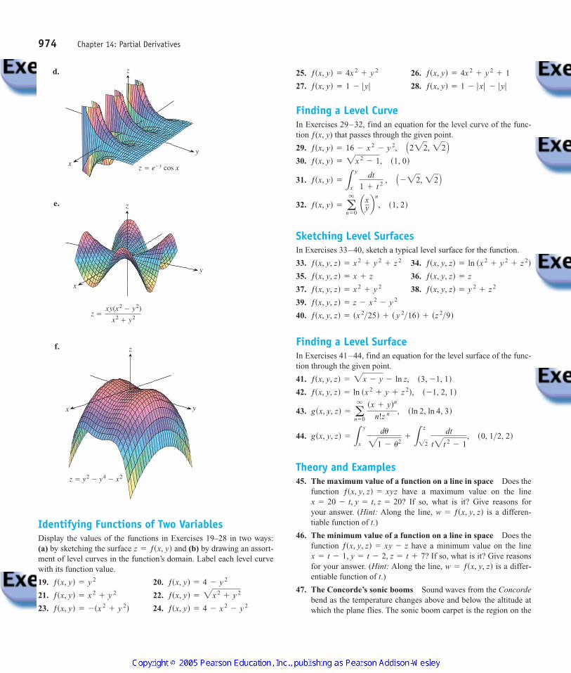
d.
e.
f.
Identifying Functions of Two VariablesDisplay the values of the functions in Exercises 19–28 in two ways:(a) by sketching the surface and (b) by drawing an assort-ment of level curves in the function’s domain. Label each level curvewith its function value.
19. 20.
21. 22.
23. 24. ƒsx, yd = 4 - x 2- y 2ƒsx, yd = -sx 2
+ y 2dƒsx, yd = 2x 2
+ y 2ƒsx, yd = x 2+ y 2
ƒsx, yd = 4 - y 2ƒsx, yd = y 2
z = ƒsx, yd
z � y2 � y4 � x2
z
x y
z �xy(x2 � y2)
x2 � y2
z
x
y
z � e–y cos xx
y
z 25. 26.
27. 28.
Finding a Level CurveIn Exercises 29–32, find an equation for the level curve of the func-tion ƒ(x, y) that passes through the given point.
29.
30.
31.
32.
Sketching Level SurfacesIn Exercises 33–40, sketch a typical level surface for the function.
33. 34.
35. 36.
37. 38.
39.
40.
Finding a Level SurfaceIn Exercises 41–44, find an equation for the level surface of the func-tion through the given point.
41.
42.
43.
44.
Theory and Examples45. The maximum value of a function on a line in space Does the
function have a maximum value on the lineIf so, what is it? Give reasons for
your answer. (Hint: Along the line, is a differen-tiable function of t.)
46. The minimum value of a function on a line in space Does thefunction have a minimum value on the line
If so, what is it? Give reasonsfor your answer. (Hint: Along the line, is a differ-entiable function of t.)
47. The Concorde’s sonic booms Sound waves from the Concordebend as the temperature changes above and below the altitude atwhich the plane flies. The sonic boom carpet is the region on the
w = ƒsx, y, zdx = t - 1, y = t - 2, z = t + 7?
ƒsx, y, zd = xy - z
w = ƒsx, y, zdx = 20 - t, y = t, z = 20?
ƒsx, y, zd = xyz
gsx, y, zd = Ly
x
du21 - u2+ L
z22
dt
t2t 2- 1
, s0, 1>2, 2d
gsx, y, zd = aq
n = 0 sx + ydn
n!z n , sln 2, ln 4, 3d
ƒsx, y, zd = ln sx 2+ y + z 2d, s -1, 2, 1d
ƒsx, y, zd = 2x - y - ln z, s3, -1, 1d
ƒsx, y, zd = sx 2>25d + s y 2>16d + sz 2>9dƒsx, y, zd = z - x 2
- y 2
ƒsx, y, zd = y 2+ z 2ƒsx, y, zd = x 2
+ y 2
ƒsx, y, zd = zƒsx, y, zd = x + z
ƒsx, y, zd = ln sx 2+ y 2
+ z 2dƒsx, y, zd = x 2+ y 2
+ z 2
ƒsx, yd = aq
n = 0 axy b
n
, s1, 2d
ƒsx, yd = Ly
x
dt
1 + t 2 , A -22, 22 Bƒsx, yd = 2x 2
- 1, s1, 0dƒsx, yd = 16 - x 2
- y 2, A222, 22 B
ƒsx, yd = 1 - ƒ x ƒ - ƒ y ƒƒsx, yd = 1 - ƒ y ƒ
ƒsx, yd = 4x 2+ y 2
+ 1ƒsx, yd = 4x 2+ y 2
974 Chapter 14: Partial Derivatives
4100 AWL/Thomas_ch14p965-1066 8/25/04 2:52 PM Page 974
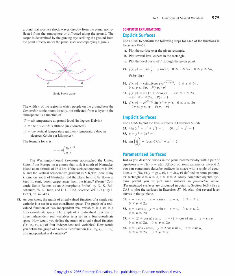
ground that receives shock waves directly from the plane, not re-flected from the atmosphere or diffracted along the ground. Thecarpet is determined by the grazing rays striking the ground fromthe point directly under the plane. (See accompanying figure.)
The width w of the region in which people on the ground hear theConcorde’s sonic boom directly, not reflected from a layer in theatmosphere, is a function of
The formula for w is
The Washington-bound Concorde approached the UnitedStates from Europe on a course that took it south of NantucketIsland at an altitude of 16.8 km. If the surface temperature is 290K and the vertical temperature gradient is 5 K km, how manykilometers south of Nantucket did the plane have to be flown tokeep its sonic boom carpet away from the island? (From “Con-corde Sonic Booms as an Atmospheric Probe” by N. K. Bal-achandra, W. L. Donn, and D. H. Rind, Science, Vol. 197 (July 1,1977), pp. 47–49.)
48. As you know, the graph of a real-valued function of a single realvariable is a set in a two-coordinate space. The graph of a real-valued function of two independent real variables is a set in athree-coordinate space. The graph of a real-valued function ofthree independent real variables is a set in a four-coordinatespace. How would you define the graph of a real-valued function
of four independent real variables? How wouldyou define the graph of a real-valued function of n independent real variables?
ƒsx1, x2, x3, Á , xndƒsx1, x2, x3, x4d
>
w = 4 aThdb1>2
.
degrees Kelvin per kilometerd. d = the vertical temperature gradient stemperature drop in
h = the Concorde’s altitude sin kilometersd T = air temperature at ground level sin degrees Kelvind
A Bw
Sonic boom carpet
COMPUTER EXPLORATIONS
Explicit SurfacesUse a CAS to perform the following steps for each of the functions inExercises 49–52.
a. Plot the surface over the given rectangle.
b. Plot several level curves in the rectangle.
c. Plot the level curve of ƒ through the given point.
49.
50.
51.
52.
Implicit SurfacesUse a CAS to plot the level surfaces in Exercises 53–56.
53. 54.
55.
56.
Parametrized SurfacesJust as you describe curves in the plane parametrically with a pair ofequations defined on some parameter interval I,you can sometimes describe surfaces in space with a triple of equa-tions defined on some parame-ter rectangle Many computer algebra sys-tems permit you to plot such surfaces in parametric mode.(Parametrized surfaces are discussed in detail in Section 16.6.) Use aCAS to plot the surfaces in Exercises 57–60. Also plot several levelcurves in the xy-plane.
57.
58.
59.
60.0 … u … 2p, 0 … y … p
x = 2 cos u cos y, y = 2 cos u sin y, z = 2 sin u, 0 … u … 2p, 0 … y … 2px = s2 + cos ud cos y, y = s2 + cos ud sin y, z = sin u, 0 … y … 2px = u cos y, y = u sin y, z = y, 0 … u … 2, 0 … y … 2px = u cos y, y = u sin y, z = u, 0 … u … 2,
a … u … b, c … y … d.x = ƒsu, yd, y = gsu, yd, z = hsu, yd
x = ƒstd, y = gstd
sin ax2b - scos yd2x 2
+ z 2= 2
x + y 2- 3z 2
= 1
x 2+ z2
= 14 ln sx 2+ y 2
+ z2d = 1
-2p … y … p, Psp, -pdƒsx, yd = e sx0.1
- yd sin sx 2+ y 2d, 0 … x … 2p,
-2p … y … 2p, Psp, pdƒsx, yd = sin sx + 2 cos yd, -2p … x … 2p, 0 … y … 5p, Ps4p, 4pdƒsx, yd = ssin xdscos yde2x2
+ y2>8, 0 … x … 5p,
Ps3p, 3pd
ƒsx, yd = x sin y
2+ y sin 2x, 0 … x … 5p 0 … y … 5p,
14.1 Functions of Several Variables 975
4100 AWL/Thomas_ch14p965-1066 8/25/04 2:53 PM Page 975
976 Chapter 14: Partial Derivatives
Limits and Continuity in Higher Dimensions
This section treats limits and continuity for multivariable functions. The definition of thelimit of a function of two or three variables is similar to the definition of the limit of afunction of a single variable but with a crucial difference, as we now see.
Limits
If the values of ƒ(x, y) lie arbitrarily close to a fixed real number L for all points (x, y) suf-ficiently close to a point we say that ƒ approaches the limit L as (x, y) approaches
This is similar to the informal definition for the limit of a function of a single vari-able. Notice, however, that if lies in the interior of ƒ’s domain, (x, y) can approach
from any direction. The direction of approach can be an issue, as in some of theexamples that follow.sx0, y0d
sx0, y0dsx0, y0d.
sx0, y0d,
14.2
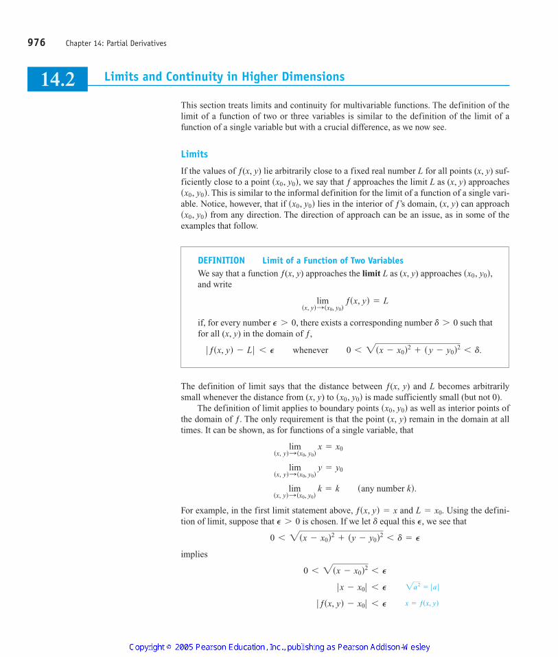
DEFINITION Limit of a Function of Two VariablesWe say that a function ƒ(x, y) approaches the limit L as (x, y) approaches and write
if, for every number there exists a corresponding number such thatfor all (x, y) in the domain of ƒ,
ƒ ƒsx, yd - L ƒ 6 P whenever 0 6 2sx - x0d2+ s y - y0d2
6 d.
d 7 0P 7 0,
limsx, yd: sx0, y0d
ƒsx, yd = L
sx0, y0d,
The definition of limit says that the distance between ƒ(x, y) and L becomes arbitrarilysmall whenever the distance from (x, y) to is made sufficiently small (but not 0).
The definition of limit applies to boundary points as well as interior points ofthe domain of ƒ. The only requirement is that the point (x, y) remain in the domain at alltimes. It can be shown, as for functions of a single variable, that
For example, in the first limit statement above, and Using the defini-tion of limit, suppose that is chosen. If we let equal this we see that
implies
ƒ ƒsx, yd - x0 ƒ 6 P
ƒ x - x0 ƒ 6 P
0 6 2sx - x0d26 P
0 6 2sx - x0d2+ sy - y0d2
6 d = P
P,dP 7 0L = x0.ƒsx, yd = x
limsx, yd: sx0, y0d
k = k sany number kd.
limsx, yd: sx0, y0d
y = y0
limsx, yd: sx0, y0d
x = x0
sx0, y0dsx0, y0d
2a2= ƒ a ƒ
x = ƒsx, yd
4100 AWL/Thomas_ch14p965-1066 8/25/04 2:53 PM Page 976
That is,
So
It can also be shown that the limit of the sum of two functions is the sum of their lim-its (when they both exist), with similar results for the limits of the differences, products,constant multiples, quotients, and powers.
limsx, yd: sx0 , y0d
ƒsx, yd = limsx, yd: sx0 , y0d
x = x0.
ƒ ƒsx, yd - x0 ƒ 6 P whenever 0 6 2sx - x0d2+ s y - y0d2
6 d.
14.2 Limits and Continuity in Higher Dimensions 977
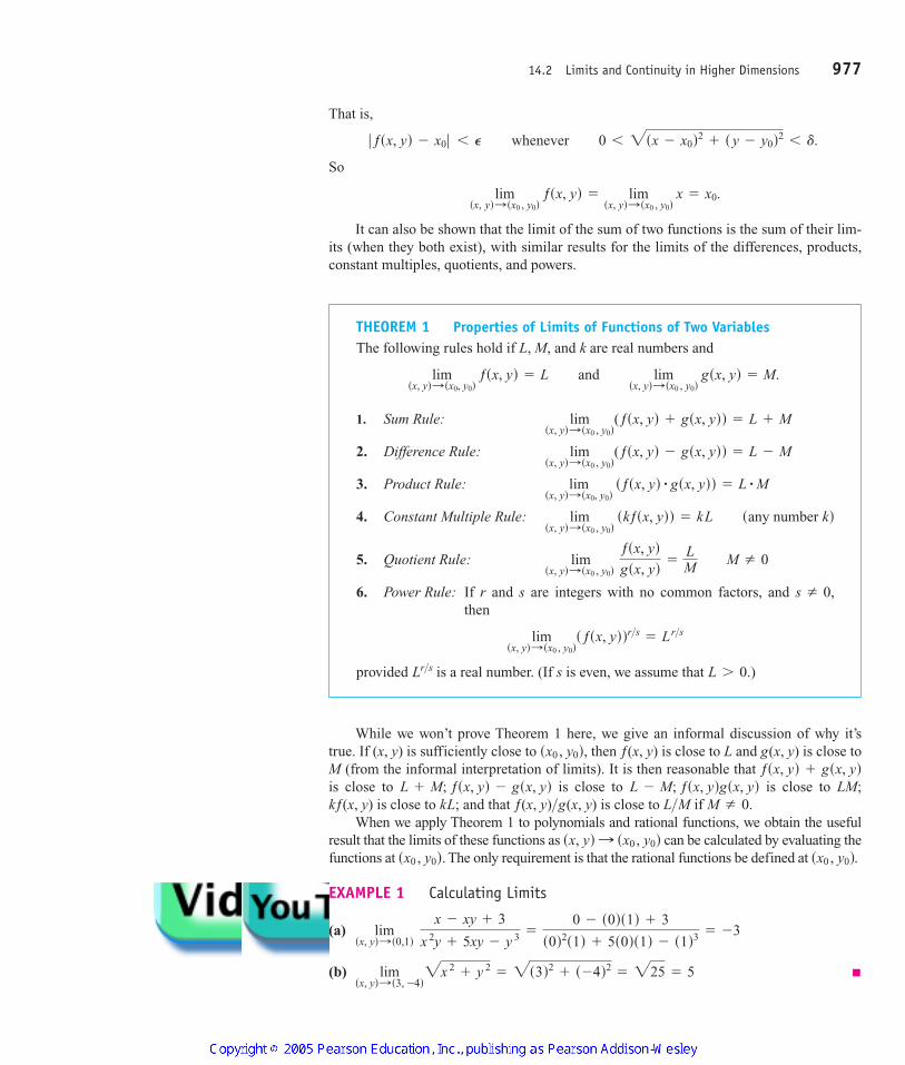
THEOREM 1 Properties of Limits of Functions of Two VariablesThe following rules hold if L, M, and k are real numbers and
1. Sum Rule:
2. Difference Rule:
3. Product Rule:
4. Constant Multiple Rule:
5. Quotient Rule:
6. Power Rule: If r and s are integers with no common factors, and then
provided is a real number. (If s is even, we assume that )L 7 0.Lr>slim
sx, yd: sx0 , y0dsƒsx, yddr>s
= Lr>s
s Z 0,
limsx, yd: sx0 , y0d
ƒsx, ydgsx, yd
=LM M Z 0
limsx, yd: sx0 , y0d
skƒsx, ydd = kL sany number kd
limsx, yd: sx0, y0d
sƒsx, yd # gsx, ydd = L # M
limsx, yd: sx0 , y0d
(ƒsx, yd - gsx, ydd = L - M
limsx, yd: sx0 , y0d
(ƒsx, yd + gsx, ydd = L + M
limsx, yd: sx0, y0d
ƒsx, yd = L and limsx, yd: sx0 , y0d
gsx, yd = M.
While we won’t prove Theorem 1 here, we give an informal discussion of why it’strue. If (x, y) is sufficiently close to then ƒ(x, y) is close to L and g(x, y) is close toM (from the informal interpretation of limits). It is then reasonable that is close to is close to is close to LM;kƒ(x, y) is close to kL; and that ƒ(x, y) g(x, y) is close to L M if
When we apply Theorem 1 to polynomials and rational functions, we obtain the usefulresult that the limits of these functions as can be calculated by evaluating thefunctions at The only requirement is that the rational functions be defined at
EXAMPLE 1 Calculating Limits
(a)
(b) limsx, yd: s3, -4d
2x 2+ y 2
= 2s3d2+ s -4d2
= 225 = 5
limsx, yd: s0,1d
x - xy + 3
x 2y + 5xy - y 3 =
0 - s0ds1d + 3
s0d2s1d + 5s0ds1d - s1d3 = -3
sx0 , y0d.sx0 , y0d.sx, yd : sx0 , y0d
M Z 0.>> L - M; ƒsx, ydgsx, ydL + M; ƒsx, yd - gsx, ydƒsx, yd + gsx, yd
sx0 , y0d,
4100 AWL/Thomas_ch14p965-1066 8/25/04 2:53 PM Page 977
EXAMPLE 2 Calculating Limits
Find
Solution Since the denominator approaches 0 as we can-not use the Quotient Rule from Theorem 1. If we multiply numerator and denominator by
however, we produce an equivalent fraction whose limit we can find:
We can cancel the factor because the path (along which ) is notin the domain of the function
EXAMPLE 3 Applying the Limit Definition
Find if it exists.
Solution We first observe that along the line the function always has value 0when Likewise, along the line the function has value 0 provided Soif the limit does exist as (x, y) approaches (0, 0), the value of the limit must be 0. To see ifthis is true, we apply the definition of limit.
Let be given, but arbitrary. We want to find a such that
or
Since we have that
4 ƒ x ƒ y 2
x 2+ y 2 … 4 ƒ x ƒ = 42x 2
… 42x 2+ y 2 .
y 2… x 2
+ y 2
4 ƒ x ƒ y 2
x 2+ y 2 6 P whenever 0 6 2x 2
+ y 26 d.
` 4xy 2
x 2+ y 2 - 0 ` 6 P whenever 0 6 2x 2
+ y 26 d
d 7 0P 7 0
x Z 0.y = 0,y Z 0.x = 0,
limsx, yd: s0,0d
4xy2
x 2+ y 2
x 2- xy2x - 2y
.
x - y = 0y = xsx - yd
= 0 A20 + 20 B = 0
= limsx, yd: s0,0d
x A2x + 2y B = lim
sx, yd: s0,0d x Ax - y B A2x + 2y B
x - y
limsx, yd: s0,0d
x 2
- xy2x - 2y= lim
sx, yd: s0,0d Ax 2
- xy B A2x + 2y BA2x - 2y B A2x + 2y B
2x + 2y,
sx, yd : s0, 0d,2x - 2y
limsx, yd: s0,0d
x2
- xy2x - 2y.
978 Chapter 14: Partial Derivatives
Cancel the nonzerofactor sx - yd.
Algebra
4100 AWL/Thomas_ch14p965-1066 8/25/04 2:53 PM Page 978
So if we choose and let we get
It follows from the definition that
Continuity
As with functions of a single variable, continuity is defined in terms of limits.
limsx, yd: s0,0d
4xy 2
x 2+ y 2 = 0.
` 4xy 2
x 2+ y 2 - 0 ` … 42x 2
+ y 26 4d = 4 aP
4b = P.
0 6 2x2+ y2
6 d,d = P>4
14.2 Limits and Continuity in Higher Dimensions 979
DEFINITION Continuous Function of Two VariablesA function ƒ(x, y) is continuous at the point if
1. ƒ is defined at
2. exists,
3.
A function is continuous if it is continuous at every point of its domain.
limsx, yd: sx0, y0d
ƒsx, yd = ƒsx0, y0d.
limsx, yd: sx0, y0d
ƒsx, ydsx0, y0d,
(x0, y0)
As with the definition of limit, the definition of continuity applies at boundary pointsas well as interior points of the domain of ƒ. The only requirement is that the point (x, y)remain in the domain at all times.
As you may have guessed, one of the consequences of Theorem 1 is that algebraic com-binations of continuous functions are continuous at every point at which all the functions in-volved are defined. This means that sums, differences, products, constant multiples, quotients,and powers of continuous functions are continuous where defined. In particular, polynomialsand rational functions of two variables are continuous at every point at which they are defined.
EXAMPLE 4 A Function with a Single Point of Discontinuity
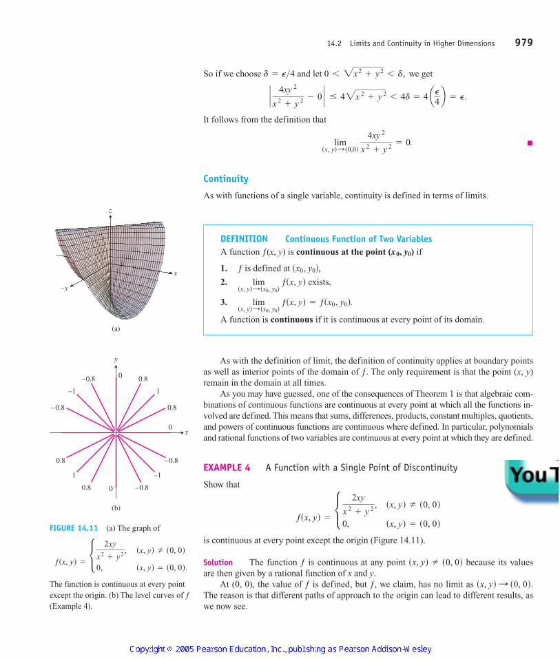
Show that
is continuous at every point except the origin (Figure 14.11).
Solution The function ƒ is continuous at any point because its valuesare then given by a rational function of x and y.
At (0, 0), the value of ƒ is defined, but ƒ, we claim, has no limit as The reason is that different paths of approach to the origin can lead to different results, aswe now see.
sx, yd : s0, 0d.
sx, yd Z s0, 0d
ƒsx, yd = L 2xy
x 2+ y 2 , sx, yd Z s0, 0d
0, sx, yd = s0, 0d
(a)
z
x
y
0
0.8
0.8
1
0
(b)
00.8
0.8
1
–y
–0.8
–1
–0.8
–0.8
–1
–0.8
x
FIGURE 14.11 (a) The graph of
The function is continuous at every pointexcept the origin. (b) The level curves of ƒ(Example 4).
ƒsx, yd = L 2xy
x2+ y2 , sx, yd Z s0, 0d
0, sx, yd = s0, 0d.
4100 AWL/Thomas_ch14p965-1066 8/25/04 2:53 PM Page 979
For every value of m, the function ƒ has a constant value on the “punctured” linebecause
Therefore, ƒ has this number as its limit as (x, y) approaches (0, 0) along the line:
This limit changes with m. There is therefore no single number we may call the limit ofƒ as (x, y) approaches the origin. The limit fails to exist, and the function is notcontinuous.
Example 4 illustrates an important point about limits of functions of two variables (oreven more variables, for that matter). For a limit to exist at a point, the limit must be thesame along every approach path. This result is analogous to the single-variable case whereboth the left- and right-sided limits had to have the same value; therefore, for functions oftwo or more variables, if we ever find paths with different limits, we know the function hasno limit at the point they approach.
limsx, yd: s0,0d
ƒsx, yd = limsx, yd: s0,0d
cƒsx, yd `y = mxd =
2m1 + m2 .
ƒsx, yd `y = mx
=
2xy
x 2+ y 2 `
y = mx=
2xsmxdx 2
+ smxd2 =
2mx 2
x 2+ m2x 2 =
2m1 + m2 .
y = mx, x Z 0,
980 Chapter 14: Partial Derivatives
Two-Path Test for Nonexistence of a LimitIf a function ƒ(x, y) has different limits along two different paths as (x, y) ap-proaches then does not exist.limsx, yd:sx0, y0d ƒsx, ydsx0, y0d,
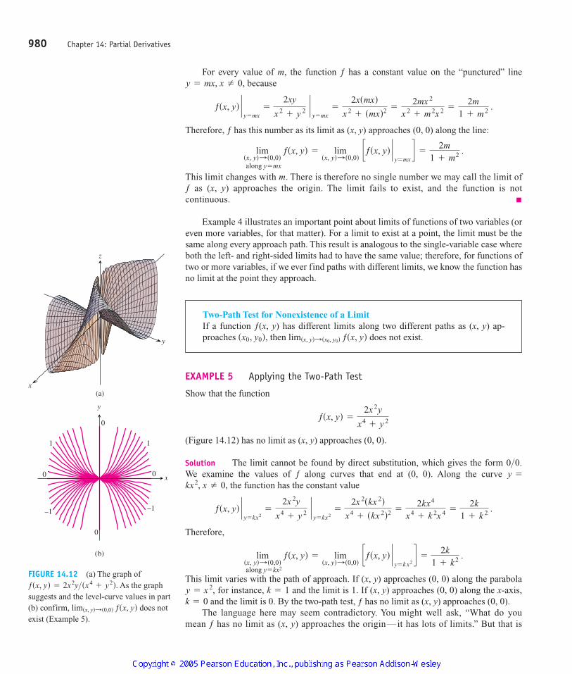
EXAMPLE 5 Applying the Two-Path Test
Show that the function
(Figure 14.12) has no limit as (x, y) approaches (0, 0).
Solution The limit cannot be found by direct substitution, which gives the form 0 0.We examine the values of ƒ along curves that end at (0, 0). Along the curve
the function has the constant value
Therefore,
This limit varies with the path of approach. If (x, y) approaches (0, 0) along the parabolafor instance, and the limit is 1. If (x, y) approaches (0, 0) along the x-axis,
and the limit is 0. By the two-path test, ƒ has no limit as (x, y) approaches (0, 0).The language here may seem contradictory. You might well ask, “What do you
mean ƒ has no limit as (x, y) approaches the origin—it has lots of limits.” But that is
k = 0k = 1y = x 2,
limsx, yd: s0,0d
ƒsx, yd = limsx, yd: s0,0d
cƒsx, yd `y = k x2
d =
2k1 + k2 .
ƒsx, yd `y = kx2
=
2x 2y
x4+ y 2 `
y = kx2=
2x 2skx 2dx4
+ skx 2d2 =
2kx4
x4+ k 2x 4 =
2k1 + k 2 .
kx2, x Z 0,y =
>
ƒsx, yd =
2x 2y
x4+ y 2
(a)
x
(b)
0
1
–1
y
1
–1
0
0
0
z
x
y
FIGURE 14.12 (a) The graph ofAs the graph
suggests and the level-curve values in part(b) confirm, does notexist (Example 5).
limsx, yd:s0,0d ƒsx, yd
ƒsx, yd = 2x2y>sx4+ y2d.
along y = mx
along y = kx2
4100 AWL/Thomas_ch14p965-1066 8/25/04 2:53 PM Page 980
the point. There is no single path-independent limit, and therefore, by the definition,does not exist.
Compositions of continuous functions are also continuous. The proof, omitted here,is similar to that for functions of a single variable (Theorem 10 in Section 2.6).
limsx, yd:s0,0d ƒsx, yd
14.2 Limits and Continuity in Higher Dimensions 981
Continuity of CompositesIf ƒ is continuous at and g is a single-variable function continuous at
then the composite function defined by is continuous at sx0, y0d.
hsx, yd = gsƒsx, yddh = g � fƒsx0, y0d,sx0, y0d
For example, the composite functions
are continuous at every point (x, y).As with functions of a single variable, the general rule is that composites of continu-
ous functions are continuous. The only requirement is that each function be continuouswhere it is applied.
Functions of More Than Two Variables
The definitions of limit and continuity for functions of two variables and the conclusionsabout limits and continuity for sums, products, quotients, powers, and composites all ex-tend to functions of three or more variables. Functions like
are continuous throughout their domains, and limits like
where P denotes the point (x, y, z), may be found by direct substitution.
Extreme Values of Continuous Functions on Closed, Bounded Sets
We have seen that a function of a single variable that is continuous throughout a closed,bounded interval [a, b] takes on an absolute maximum value and an absolute minimumvalue at least once in [a, b]. The same is true of a function that is continuouson a closed, bounded set R in the plane (like a line segment, a disk, or a filled-in triangle).The function takes on an absolute maximum value at some point in R and an absolute min-imum value at some point in R.
Theorems similar to these and other theorems of this section hold for functions ofthree or more variables. A continuous function for example, must take onabsolute maximum and minimum values on any closed, bounded set (solid ball or cube,spherical shell, rectangular solid) on which it is defined.
We learn how to find these extreme values in Section 14.7, but first we need to studyderivatives in higher dimensions. That is the topic of the next section.
w = ƒsx, y, zd,
z = ƒsx, yd
limP: s1,0,-1d
e x + z
z 2+ cos 2xy
=
e1 - 1
s -1d2+ cos 0
=12
,
ln sx + y + zd and y sin zx - 1
e x - y, cos xy
x 2+ 1
, ln s1 + x 2y 2d
4100 AWL/Thomas_ch14p965-1066 8/25/04 2:53 PM Page 981
982 Chapter 14: Partial Derivatives
EXERCISES 14.2
Limits with Two VariablesFind the limits in Exercises 1–12.
1. 2.
3. 4.
5. 6.
7. 8.
9. 10.
11. 12.
Limits of QuotientsFind the limits in Exercises 13–20 by rewriting the fractions first.
13. 14.
15.
16.
17.
18. 19.
20.
Limits with Three VariablesFind the limits in Exercises 21–26.
21. 22.
23.
24. 25.
26. limP: s0, -2,0d
ln2x 2+ y 2
+ z 2
limP: sp,0,3d
ze-2y cos 2xlimP: s-1>4,p>2,2d
tan-1 xyz
limP: s3,3,0d
ssin2 x + cos2 y + sec2 zd
limP: s1,-1,-1d
2xy + yz
x 2+ z 2lim
P: s1,3,4d a1x +
1y +
1z b
limsx, yd: s4,3d
2x - 2y + 1
x - y - 1
limsx, yd: s2,0d
22x - y - 2
2x - y - 4lim
sx, yd: s2,2d
x + y - 42x + y - 2
limsx, yd: s0,0d
x - y + 22x - 22y2x - 2y
limsx, yd: s2, -4d
y + 4
x2y - xy + 4x 2- 4x
limsx, yd: s1,1d
xy - y - 2x + 2
x - 1
limsx, yd: s1,1d
x 2
- y 2
x - ylimsx, yd: s1,1d
x 2
- 2xy + y 2
x - y
limsx, yd: sp>2,0d
cos y + 1
y - sin xlim
sx, yd: s1,0d
x sin y
x 2+ 1
limsx, yd: s1,1d
cos23 ƒ xy ƒ - 1limsx, yd: s0,0d
e y sin x
x
limsx, yd: s1,1d
ln ƒ 1 + x 2 y 2ƒlim
sx, yd: s0,ln 2d e x - y
limsx, yd: s0,0d
cos x 2
+ y 3
x + y + 1lim
sx, yd: s0,p>4d sec x tan y
limsx, yd: s2, -3d
a1x +
1y b
2
limsx, yd: s3,4d
2x 2+ y 2
- 1
limsx, yd: s0,4d
x2y
limsx, yd: s0,0d
3x 2
- y 2+ 5
x 2+ y 2
+ 2
Continuity in the PlaneAt what points (x, y) in the plane are the functions in Exercises 27–30continuous?
27. a. b.
28. a. b.
29. a. b.
30. a. b.
Continuity in SpaceAt what points (x, y, z) in space are the functions in Exercises 31–34continuous?
31. a.
b.
32. a. b.
33. a. b.
34. a. b.
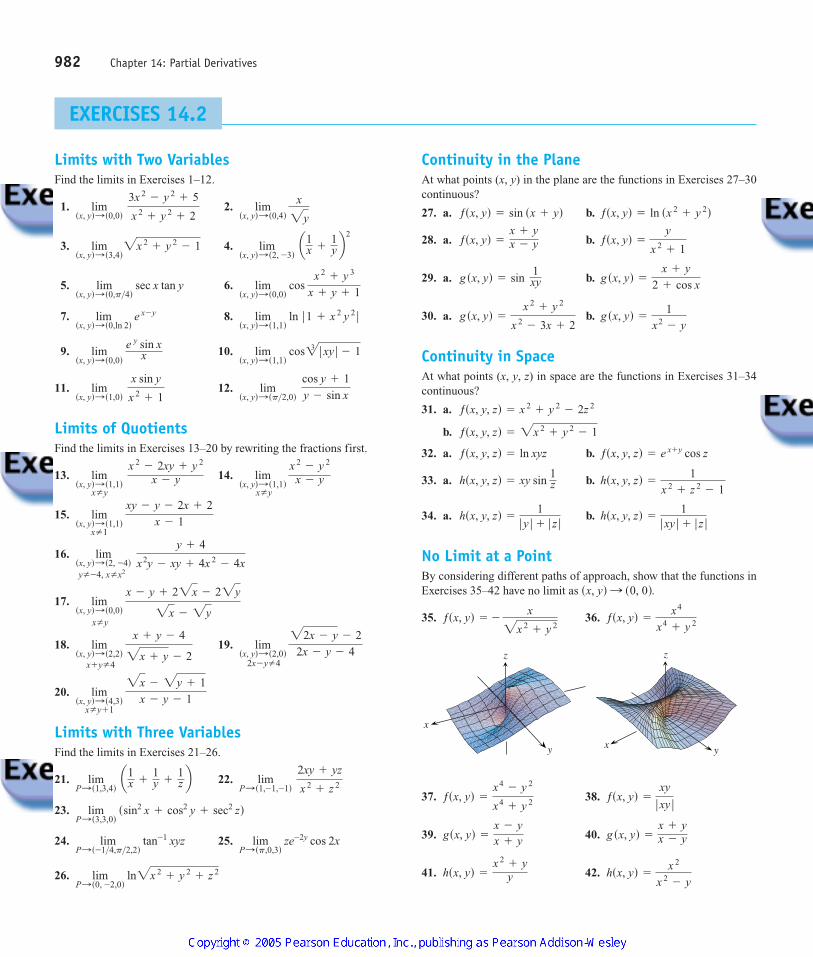
No Limit at a PointBy considering different paths of approach, show that the functions inExercises 35–42 have no limit as
35. 36.
37. 38.
39. 40.
41. 42. hsx, yd =
x 2
x 2- y
hsx, yd =
x 2+ yy
g sx, yd =
x + yx - ygsx, yd =
x - yx + y
ƒsx, yd =
xy
ƒ xy ƒ
ƒsx, yd =
x4- y 2
x4+ y 2
z
yx
z
y
x
ƒsx, yd =
x4
x4+ y 2ƒsx, yd = -
x2x 2+ y 2
sx, yd : s0, 0d.
hsx, y, zd =
1ƒ xy ƒ + ƒ z ƒ
hsx, y, zd =
1ƒ y ƒ + ƒ z ƒ
hsx, y, zd =
1x 2
+ z 2- 1
hsx, y, zd = xy sin 1z
ƒsx, y, zd = e x + y cos zƒsx, y, zd = ln xyz
ƒsx, y, zd = 2x 2+ y 2
- 1
ƒsx, y, zd = x 2+ y 2
- 2z 2
g sx, yd =
1x2
- yg sx, yd =
x 2+ y 2
x 2- 3x + 2
g sx, yd =
x + y
2 + cos xg sx, yd = sin
1xy
ƒsx, yd =
y
x 2+ 1
ƒsx, yd =
x + yx - y
ƒsx, yd = ln sx 2+ y 2dƒsx, yd = sin sx + yd
x Z y
x Z y
x Z y
x Z 1
y Z -4, x Z x2
x + y Z 4 2x - y Z 4
x Z y + 1
4100 AWL/Thomas_ch14p965-1066 8/25/04 2:53 PM Page 982
Theory and Examples43. If must ƒ be defined at Give
reasons for your answer.
44. If what can you say about
if ƒ is continuous at If ƒ is not continuous at Give reasons for your answer.
The Sandwich Theorem for functions of two variables states that iffor all in a disk centered
at and if g and h have the same finite limit L asthen
Use this result to support your answers to the questions in Exercises45–48.
45. Does knowing that
tell you anything about
Give reasons for your answer.
46. Does knowing that
tell you anything about
Give reasons for your answer.
47. Does knowing that tell you anything about
Give reasons for your answer.
48. Does knowing that tell you anything about
Give reasons for your answer.
49. (Continuation of Example 4.)
a. Reread Example 4. Then substitute into the formula
ƒsx, yd `y = mx
=
2m
1 + m2
m = tan u
limsx, yd: s0,0d
x cos 1y ?
ƒ cos s1>yd ƒ … 1
limsx, yd: s0,0d
y sin 1x ?
ƒ sin s1>xd ƒ … 1
limsx, yd: s0,0d
4 - 4 cos 2ƒ xy ƒ
ƒ xy ƒ
?
2 ƒ xy ƒ -
x2y2
66 4 - 4 cos 2ƒ xy ƒ 6 2 ƒ xy ƒ
limsx, yd: s0,0d
tan-1 xy
xy ?
1 -
x 2y 2
36
tan-1 xyxy 6 1
limsx, yd: sx0 , y0d
ƒsx, yd = L.
sx, yd : sx0 , y0d,sx0 , y0d
sx, yd Z sx0 , y0dgsx, yd … ƒsx, yd … hsx, yd
sx0 , y0d?sx0 , y0d?
limsx, yd: sx0 , y0d
ƒsx, yd
ƒsx0 , y0d = 3,
sx0 , y0d?limsx, yd:sx0 , y0d ƒsx, yd = L,
and simplify the result to show how the value of ƒ varies withthe line’s angle of inclination.
b. Use the formula you obtained in part (a) to show that the limitof ƒ as along the line varies from to 1 depending on the angle of approach.
50. Continuous extension Define ƒ(0, 0) in a way that extends
to be continuous at the origin.
Changing to Polar CoordinatesIf you cannot make any headway with in rectan-gular coordinates, try changing to polar coordinates. Substitute
and investigate the limit of the resulting ex-pression as In other words, try to decide whether there exists anumber L satisfying the following criterion:
Given there exists a such that for all r and
(1)
If such an L exists, then
For instance,
To verify the last of these equalities, we need to show that Equation (1)is satisfied with and That is, we need to showthat given any there exists a such that for all r and
Since
the implication holds for all r and if we take In contrast,
takes on all values from 0 to 1 regardless of how small is, so thatdoes not exist.
In each of these instances, the existence or nonexistence of the limitas is fairly clear. Shifting to polar coordinates does not alwayshelp, however, and may even tempt us to false conclusions. For example,the limit may exist along every straight line (or ray) andyet fail to exist in the broader sense. Example 4 illustrates this point. Inpolar coordinates, becomes
ƒsr cos u, r sin ud =
r cos u sin 2u
r 2 cos4 u + sin2 u
ƒsx, yd = s2x 2yd>sx4+ y 2d
u = constant
r : 0
limsx, yd:s0,0d x2>sx 2
+ y 2dƒ r ƒ
x 2
x 2+ y 2 =
r 2 cos2 u
r 2 = cos2 u
d = P.u
ƒ r cos3 u ƒ = ƒ r ƒ ƒ cos3 u ƒ … ƒ r ƒ# 1 = ƒ r ƒ ,
ƒ r ƒ 6 d Q ƒ r cos3 u - 0 ƒ 6 P.
u,d 7 0P 7 0L = 0.ƒsr, ud = r cos3 u
limsx, yd: s0,0d
x3
x 2+ y 2 = lim
r:0 r 3 cos3 u
r 2 = limr:0
r cos3 u = 0.
limsx, yd: s0,0d
ƒsx, yd = limr:0
ƒsr, ud = L.
ƒ r ƒ 6 d Q ƒ ƒsr, ud - L ƒ 6 P.
u,d 7 0P 7 0,
r : 0.x = r cos u, y = r sin u,
limsx, yd:s0,0d ƒsx, yd
ƒsx, yd = xy x 2
- y 2
x 2+ y 2
-1y = mxsx, yd : s0, 0d
14.2 Limits and Continuity in Higher Dimensions 983
4100 AWL/Thomas_ch14p965-1066 8/25/04 2:53 PM Page 983
for If we hold constant and let the limit is 0. On thepath however, we have and
In Exercises 51–56, find the limit of ƒ as or show thatthe limit does not exist.
51. 52.
53. 54.
55.
56.
In Exercises 57 and 58, define ƒ(0, 0) in a way that extends ƒ tobe continuous at the origin.
57.
58. ƒsx, yd =
3x 2y
x 2+ y 2
ƒsx, yd = ln a3x 2- x 2y 2
+ 3y 2
x 2+ y 2 b
ƒsx, yd =
x 2- y 2
x 2+ y 2
ƒsx, yd = tan-1 a ƒ x ƒ + ƒ y ƒ
x 2+ y 2 b
ƒsx, yd =
2x
x 2+ x + y 2ƒsx, yd =
y 2
x 2+ y 2
ƒsx, yd = cos a x 3- y 3
x 2+ y 2 bƒsx, yd =
x 3- xy 2
x 2+ y 2
sx, yd : s0, 0d
=
2r cos2 u sin u
2r 2 cos4 u=
r sin u
r 2 cos2 u= 1.
ƒsr cos u, r sin ud =
r cos u sin 2u
r 2 cos4 u + sr cos2 ud2
r sin u = r 2 cos2 uy = x 2,r : 0,ur Z 0. Using the Definition
Each of Exercises 59–62 gives a function ƒ(x, y) and a positive num-ber In each exercise, show that there exists a such that for all(x, y),
59.
60.
61.
62.
Each of Exercises 63–66 gives a function ƒ(x, y, z) and a positive num-ber In each exercise, show that there exists a such that for all(x, y, z),
63.
64.
65.
66.
67. Show that is continuous at every point
68. Show that is continuous at the origin.ƒsx, y, zd = x 2+ y 2
+ z 2
sx0 , y0 , z0d.ƒsx, y, zd = x + y - z
ƒsx, y, zd = tan2 x + tan2 y + tan2 z, P = 0.03
ƒsx, y, zd =
x + y + z
x 2+ y 2
+ z 2+ 1
, P = 0.015
ƒsx, y, zd = xyz, P = 0.008
ƒsx, y, zd = x 2+ y 2
+ z 2, P = 0.015
2x 2+ y 2
+ z 26 d Q ƒ ƒsx, y, zd - ƒs0, 0, 0d ƒ 6 P.
d 7 0P.
ƒsx, yd = sx + yd>s2 + cos xd, P = 0.02
ƒsx, yd = sx + yd>sx2+ 1d, P = 0.01
ƒsx, yd = y>sx2+ 1d, P = 0.05
ƒsx, yd = x2+ y2, P = 0.01
2x 2+ y 2
6 d Q ƒ ƒsx, yd - ƒs0, 0d ƒ 6 P.
d 7 0P.
d-P
984 Chapter 14: Partial Derivatives
4100 AWL/Thomas_ch14p965-1066 8/25/04 2:53 PM Page 984
984 Chapter 14: Partial Derivatives
Partial Derivatives
The calculus of several variables is basically single-variable calculus applied to severalvariables one at a time. When we hold all but one of the independent variables of afunction constant and differentiate with respect to that one variable, we get a “partial”derivative. This section shows how partial derivatives are defined and interpreted geo-metrically, and how to calculate them by applying the rules for differentiating functionsof a single variable.
Partial Derivatives of a Function of Two Variables
If is a point in the domain of a function ƒ(x, y), the vertical plane will cutthe surface in the curve (Figure 14.13). This curve is the graphof the function in the plane The horizontal coordinate in this plane isx; the vertical coordinate is z. The y-value is held constant at , so y is not a variable.
We define the partial derivative of ƒ with respect to x at the point as the ordi-nary derivative of with respect to x at the point To distinguish partial de-rivatives from ordinary derivatives we use the symbol rather than the d previously used.0
x = x0.ƒsx, y0dsx0, y0d
y0
y = y0.z = ƒsx, y0dz = ƒsx, y0dz = ƒsx, yd
y = y0sx0 , y0d
14.3
4100 AWL/Thomas_ch14p965-1066 8/25/04 2:53 PM Page 984
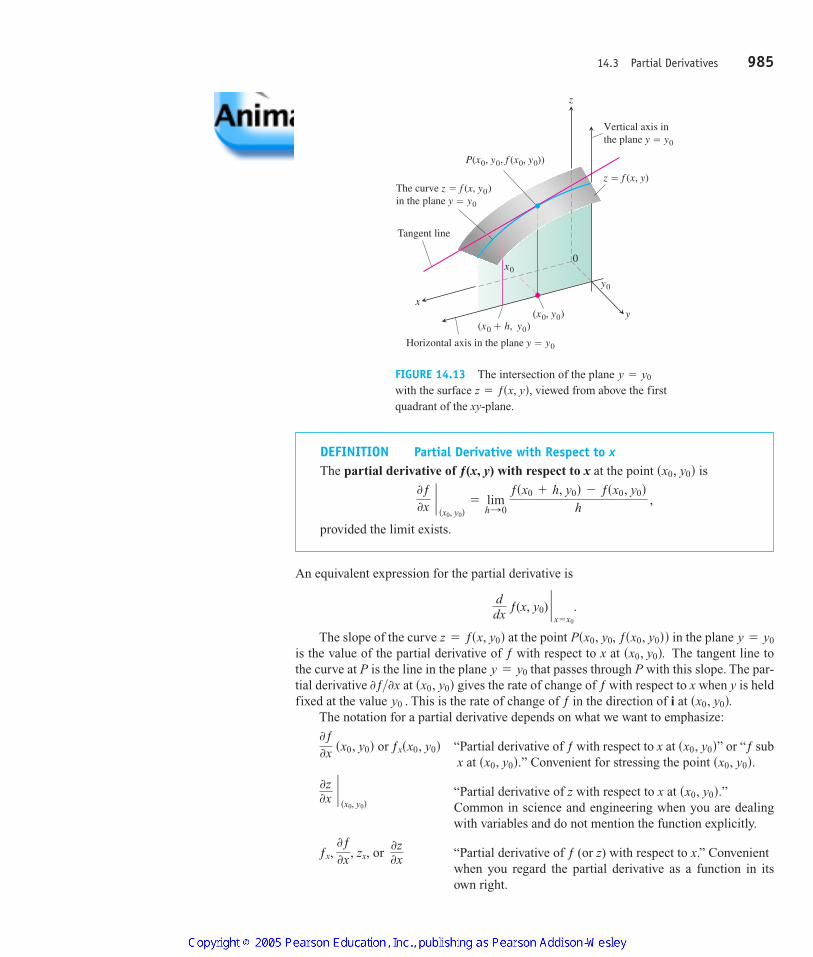
An equivalent expression for the partial derivative is
The slope of the curve at the point in the plane is the value of the partial derivative of ƒ with respect to x at The tangent line tothe curve at P is the line in the plane that passes through P with this slope. The par-tial derivative at gives the rate of change of ƒ with respect to x when y is heldfixed at the value This is the rate of change of ƒ in the direction of i at
The notation for a partial derivative depends on what we want to emphasize:
or “Partial derivative of ƒ with respect to x at ” or “ƒ subx at ” Convenient for stressing the point
“Partial derivative of z with respect to x at ”Common in science and engineering when you are dealingwith variables and do not mention the function explicitly.
or “Partial derivative of ƒ (or z) with respect to x.” Convenientwhen you regard the partial derivative as a function in itsown right.
0z0xƒx,
0ƒ0x , zx,
sx0, y0d.0z0x `
sx0, y0d
sx0, y0d.sx0, y0d.sx0, y0dƒxsx0, y0d
0ƒ0x sx0, y0d
sx0, y0d.y0 .sx0, y0d0ƒ>0x
y = y0
sx0, y0d.y = y0Psx0, y0, ƒsx0, y0ddz = ƒsx, y0d
ddx
ƒ(x, y0) `x = x0
.
14.3 Partial Derivatives 985
xy
z
0
Tangent line
The curve z � f (x, y0)in the plane y � y0
P(x0, y0, f (x0, y0))
Vertical axis inthe plane y � y0
z � f (x, y)
y0
x0
Horizontal axis in the plane y � y0
(x0 � h, y0)(x0, y0)
FIGURE 14.13 The intersection of the plane with the surface viewed from above the firstquadrant of the xy-plane.
z = ƒsx, yd,y = y0
DEFINITION Partial Derivative with Respect to xThe partial derivative of ƒ(x, y) with respect to x at the point is
provided the limit exists.
0ƒ0x `
sx0, y0d= lim
h:0 ƒsx0 + h, y0d - ƒsx0, y0d
h,
sx0, y0d
4100 AWL/Thomas_ch14p965-1066 8/25/04 2:53 PM Page 985
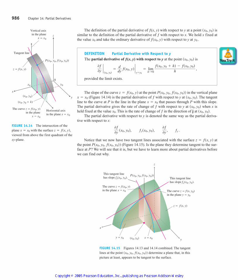
The slope of the curve at the point in the vertical plane(Figure 14.14) is the partial derivative of ƒ with respect to y at The tangent
line to the curve at P is the line in the plane that passes through P with this slope.The partial derivative gives the rate of change of ƒ with respect to y at when x isheld fixed at the value This is the rate of change of ƒ in the direction of j at
The partial derivative with respect to y is denoted the same way as the partial deriva-tive with respect to x:
Notice that we now have two tangent lines associated with the surface atthe point (Figure 14.15). Is the plane they determine tangent to the sur-face at P? We will see that it is, but we have to learn more about partial derivatives beforewe can find out why.
Psx0, y0, ƒsx0, y0ddz = ƒsx, yd
0ƒ0y sx0, y0d, ƒysx0, y0d, 0ƒ
0y , ƒy .
sx0, y0d.x0.sx0, y0d
x = x0
sx0, y0d.x = x0
Psx0, y0, ƒsx0, y0ddz = ƒsx0, yd
The definition of the partial derivative of ƒ(x, y) with respect to y at a point issimilar to the definition of the partial derivative of ƒ with respect to x. We hold x fixed atthe value and take the ordinary derivative of with respect to y at y0 .ƒsx0, ydx0
sx0, y0d
986 Chapter 14: Partial Derivatives
DEFINITION Partial Derivative with Respect to yThe partial derivative of ƒ(x, y) with respect to y at the point is
provided the limit exists.
0ƒ0y `
sx0, y0d=
ddy
ƒsx0, yd `y = y0
= limh:0
ƒsx0, y0 + hd - ƒsx0, y0d
h,
sx0, y0d
x
z
y
P(x0, y0, f (x0, y0))
y0x0
(x0, y0)
(x0, y0 � k)
The curve z � f (x0, y)in the plane
x � x0
Horizontal axisin the plane x � x0
z � f (x, y)
Tangent line
Vertical axisin the plane
x � x0
0
FIGURE 14.14 The intersection of theplane with the surface viewed from above the first quadrant of thexy-plane.
z = ƒsx, yd,x = x0
x
y
z
This tangent linehas slope fy(x0, y0). This tangent line
has slope fx(x0, y0).
The curve z � f (x, y0)in the plane y � y0
z � f (x, y)
x � x0y � y0 (x0, y0)
The curve z � f (x0, y)in the plane x � x0
P(x0, y0, f (x0, y0))
FIGURE 14.15 Figures 14.13 and 14.14 combined. The tangentlines at the point determine a plane that, in thispicture at least, appears to be tangent to the surface.
sx0, y0, ƒsx0, y0dd
4100 AWL/Thomas_ch14p965-1066 8/25/04 2:53 PM Page 986
Calculations
The definitions of and give us two different ways of differentiating ƒ at apoint: with respect to x in the usual way while treating y as a constant and with respect to yin the usual way while treating x as constant. As the following examples show, the valuesof these partial derivatives are usually different at a given point
EXAMPLE 1 Finding Partial Derivatives at a Point
Find the values of and at the point if
Solution To find we treat y as a constant and differentiate with respect to x:
The value of at is To find we treat x as a constant and differentiate with respect to y:
The value of at is
EXAMPLE 2 Finding a Partial Derivative as a Function
Find if
Solution We treat x as a constant and ƒ as a product of y and sin xy:
= s y cos xyd 0
0y sxyd + sin xy = xy cos xy + sin xy.
0ƒ0y =
0
0y s y sin xyd = y 0
0y sin xy + ssin xyd 0
0y s yd
ƒsx, yd = y sin xy.0ƒ>0y
3s4d + 1 = 13.s4, -5d0ƒ>0y
0ƒ0y =
0
0y sx 2+ 3xy + y - 1d = 0 + 3 # x # 1 + 1 - 0 = 3x + 1.
0ƒ>0y,2s4d + 3s -5d = -7.s4, -5d0ƒ>0x
0ƒ0x =
0
0x sx 2+ 3xy + y - 1d = 2x + 3 # 1 # y + 0 - 0 = 2x + 3y.
0ƒ>0x,
ƒsx, yd = x2+ 3xy + y - 1.
s4, -5d0ƒ>0y0ƒ>0x
sx0, y0d.
0ƒ>0y0ƒ>0x
14.3 Partial Derivatives 987
USING TECHNOLOGY Partial Differentiation
A simple grapher can support your calculations even in multiple dimensions. If youspecify the values of all but one independent variable, the grapher can calculate partialderivatives and can plot traces with respect to that remaining variable. Typically, a CAScan compute partial derivatives symbolically and numerically as easily as it can computesimple derivatives. Most systems use the same command to differentiate a function,regardless of the number of variables. (Simply specify the variable with which differenti-ation is to take place).
EXAMPLE 3 Partial Derivatives May Be Different Functions
Find and if
ƒsx, yd =
2yy + cos x .
ƒyƒx
4100 AWL/Thomas_ch14p965-1066 8/25/04 2:53 PM Page 987
Solution We treat ƒ as a quotient. With y held constant, we get
With x held constant, we get
Implicit differentiation works for partial derivatives the way it works for ordinaryderivatives, as the next example illustrates.
EXAMPLE 4 Implicit Partial Differentiation
Find if the equation
defines z as a function of the two independent variables x and y and the partial derivativeexists.
Solution We differentiate both sides of the equation with respect to x, holding y con-stant and treating z as a differentiable function of x:
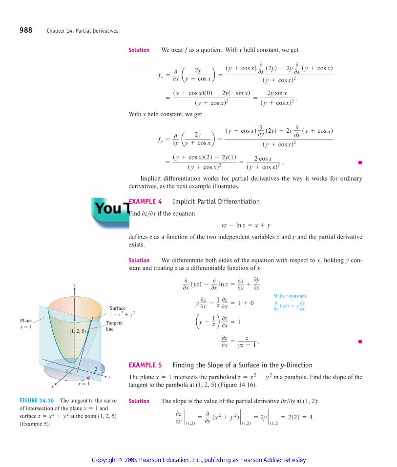
EXAMPLE 5 Finding the Slope of a Surface in the y-Direction
The plane intersects the paraboloid in a parabola. Find the slope of thetangent to the parabola at (1, 2, 5) (Figure 14.16).
Solution The slope is the value of the partial derivative at (1, 2):
0z0y `
s1,2d=
0
0y sx 2+ y 2d `
s1,2d= 2y `
s1,2d= 2s2d = 4.
0z>0y
z = x 2+ y 2x = 1
0z0x =
zyz - 1
.
ay -1z b
0z0x = 1
y 0z0x -
1z
0z0x = 1 + 0
0
0x s yzd -
0
0x ln z =
0x0x +
0y0x
yz - ln z = x + y
0z>0x
=
s y + cos xds2d - 2ys1ds y + cos xd2 =
2 cos xs y + cos xd2 .
ƒy =0
0y a 2yy + cos x b =
s y + cos xd 0
0y s2yd - 2y 0
dy s y + cos xd
s y + cos xd2
=
s y + cos xds0d - 2ys -sin xds y + cos xd2 =
2y sin x
s y + cos xd2 .
ƒx =0
0x a 2yy + cos x b =
s y + cos xd 0
0x s2yd - 2y 0
0x s y + cos xd
s y + cos xd2
988 Chapter 14: Partial Derivatives
With y constant,0
0x s yzd = y
0z0x
.
x
y1 2
(1, 2, 5)
z
Surfacez � x2 � y2
x � 1
Tangentline
Planex � 1
FIGURE 14.16 The tangent to the curveof intersection of the plane andsurface at the point (1, 2, 5)(Example 5).
z = x 2+ y 2
x = 1
4100 AWL/Thomas_ch14p965-1066 9/2/04 11:09 AM Page 988
As a check, we can treat the parabola as the graph of the single-variable functionin the plane and ask for the slope at The slope,
calculated now as an ordinary derivative, is
Functions of More Than Two Variables
The definitions of the partial derivatives of functions of more than two independentvariables are like the definitions for functions of two variables. They are ordinaryderivatives with respect to one variable, taken while the other independent variables areheld constant.
EXAMPLE 6 A Function of Three Variables
If x, y, and z are independent variables and
then
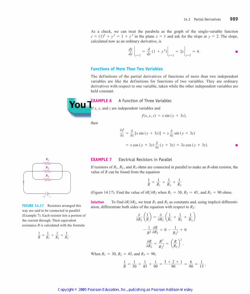
EXAMPLE 7 Electrical Resistors in Parallel
If resistors of and ohms are connected in parallel to make an R-ohm resistor, thevalue of R can be found from the equation
(Figure 14.17). Find the value of when and ohms.
Solution To find we treat and as constants and, using implicit differenti-ation, differentiate both sides of the equation with respect to
When and
1R
=130
+145
+190
=
3 + 2 + 190
=
690
=1
15,
R3 = 90,R1 = 30, R2 = 45,
0R0R2
=R2
R22 = a R
R2b2
.
-1
R2 0R0R2
= 0 -1
R22 + 0
0
0R2 a1
Rb =
0
0R2 a 1
R1+
1R2
+1R3b
R2 :R3R10R>0R2,
R3 = 90R1 = 30, R2 = 45,0R>0R2
1R
=1R1
+1R2
+1R3
R3R1, R2 ,
= x cos s y + 3zd 0
0z s y + 3zd = 3x cos s y + 3zd.
0ƒ0z =
0
0z [x sin s y + 3zd] = x 0
0z sin s y + 3zd
ƒsx, y, zd = x sin s y + 3zd,
dzdy
`y = 2
=
ddy
s1 + y 2d `y = 2
= 2y `y = 2
= 4.
y = 2.x = 1z = s1d2+ y 2
= 1 + y 2
14.3 Partial Derivatives 989
� �
R3
R2
R1
FIGURE 14.17 Resistors arranged thisway are said to be connected in parallel(Example 7). Each resistor lets a portion ofthe current through. Their equivalentresistance R is calculated with the formula
1R
=
1R1
+
1R2
+
1R3
.
4100 AWL/Thomas_ch14p965-1066 8/25/04 2:53 PM Page 989
so and
Partial Derivatives and Continuity
A function ƒ(x, y) can have partial derivatives with respect to both x and y at a point with-out the function being continuous there. This is different from functions of a single vari-able, where the existence of a derivative implies continuity. If the partial derivatives ofƒ(x, y) exist and are continuous throughout a disk centered at however, then ƒ iscontinuous at as we see at the end of this section.
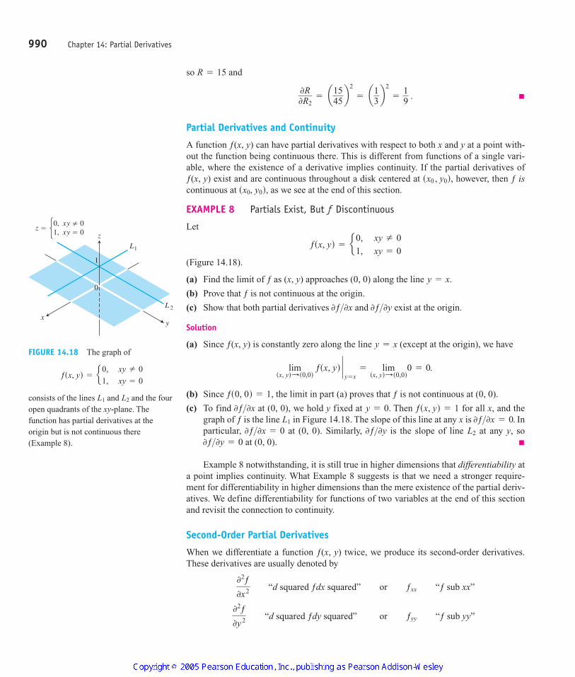
EXAMPLE 8 Partials Exist, But ƒ Discontinuous
Let
(Figure 14.18).
(a) Find the limit of ƒ as (x, y) approaches (0, 0) along the line
(b) Prove that ƒ is not continuous at the origin.
(c) Show that both partial derivatives and exist at the origin.
Solution
(a) Since ƒ(x, y) is constantly zero along the line (except at the origin), we have
(b) Since the limit in part (a) proves that ƒ is not continuous at (0, 0).
(c) To find at (0, 0), we hold y fixed at Then for all x, and thegraph of ƒ is the line in Figure 14.18. The slope of this line at any x is Inparticular, at (0, 0). Similarly, is the slope of line at any y, so
at (0, 0).
Example 8 notwithstanding, it is still true in higher dimensions that differentiability ata point implies continuity. What Example 8 suggests is that we need a stronger require-ment for differentiability in higher dimensions than the mere existence of the partial deriv-atives. We define differentiability for functions of two variables at the end of this sectionand revisit the connection to continuity.
Second-Order Partial Derivatives
When we differentiate a function ƒ(x, y) twice, we produce its second-order derivatives.These derivatives are usually denoted by
02ƒ
0y2 “d squared ƒdy squared” or ƒyy “ƒ sub yy”
02ƒ
0x2 “d squared ƒdx squared” or ƒxx “ƒ sub xx”
0ƒ>0y = 0L20ƒ>0y0ƒ>0x = 0
0ƒ>0x = 0.L1
ƒsx, yd = 1y = 0.0ƒ>0x
ƒs0, 0d = 1,
limsx, yd: s0,0d
ƒsx, yd `y = x
= limsx, yd: s0,0d
0 = 0.
y = x
0ƒ>0y0ƒ>0x
y = x.
ƒsx, yd = e0, xy Z 0
1, xy = 0
sx0, y0d,sx0 , y0d,
0R0R2
= a1545b2
= a13b2
=19
.
R = 15
990 Chapter 14: Partial Derivatives
y
z
x
0
1
L1
L 2
z �0, xy � 01, xy � 0
FIGURE 14.18 The graph of
consists of the lines and and the fouropen quadrants of the xy-plane. Thefunction has partial derivatives at theorigin but is not continuous there(Example 8).
L2L1
ƒsx, yd = e0, xy Z 0
1, xy = 0
4100 AWL/Thomas_ch14p965-1066 8/25/04 2:53 PM Page 990
The defining equations are
and so on. Notice the order in which the derivatives are taken:
EXAMPLE 9 Finding Second-Order Partial Derivatives
If find
Solution
So So
The Mixed Derivative Theorem
You may have noticed that the “mixed” second-order partial derivatives
in Example 9 were equal. This was not a coincidence. They must be equal wheneverand are continuous, as stated in the following theorem.ƒyxƒ, ƒx , ƒy , ƒxy ,
02ƒ
0y0x and 02ƒ
0x0y
0
2ƒ
0y2 =
0
0y a0ƒ0y b = -x cos y.
02ƒ
0x2 =
0
0x a0ƒ0x b = ye x.
0
2ƒ0x0y =
0
0x a0ƒ0y b = -sin y + e x
02ƒ
0y0x =
0
0y a0ƒ0x b = -sin y + e x
= -x sin y + e x = cos y + ye x
0ƒ0y =
0
0y sx cos y + ye xd 0ƒ0x =
0
0x sx cos y + ye xd
02ƒ
0x2 , 02ƒ
0y0x , 02ƒ
0y2 , and 02ƒ
0x0y .
ƒsx, yd = x cos y + yex,
ƒyx = sƒydx Means the same thing.
02ƒ
0x0y Differentiate first with respect to y, then with respect to x.
02ƒ
0x2 =0
0x a0ƒ0x b , 0
2ƒ0x0y =
0
0x a0ƒ0y b ,
02ƒ
0y0x “d squared ƒdy dx” or ƒxy “ƒ sub xy”
02ƒ
0x0y “d squared ƒdx dy” or ƒyx “ƒ sub yx”
14.3 Partial Derivatives 991
HISTORICAL BIOGRAPHY
Pierre-Simon Laplace(1749–1827)
THEOREM 2 The Mixed Derivative TheoremIf ƒ(x, y) and its partial derivatives and are defined throughout anopen region containing a point (a, b) and are all continuous at (a, b), then
ƒxysa, bd = ƒyxsa, bd.
ƒyxƒx , ƒy , ƒxy ,
4100 AWL/Thomas_ch14p965-1066 8/25/04 2:53 PM Page 991
Theorem 2 is also known as Clairaut’s Theorem, named after the French mathemati-cian Alexis Clairaut who discovered it. A proof is given in Appendix 7. Theorem 2 saysthat to calculate a mixed second-order derivative, we may differentiate in either order, pro-vided the continuity conditions are satisfied. This can work to our advantage.
EXAMPLE 10 Choosing the Order of Differentiation
Find if
Solution The symbol tells us to differentiate first with respect to y and thenwith respect to x. If we postpone the differentiation with respect to y and differentiate firstwith respect to x, however, we get the answer more quickly. In two steps,
If we differentiate first with respect to y, we obtain as well.
Partial Derivatives of Still Higher Order
Although we will deal mostly with first- and second-order partial derivatives, becausethese appear the most frequently in applications, there is no theoretical limit to how manytimes we can differentiate a function as long as the derivatives involved exist. Thus, we getthird- and fourth-order derivatives denoted by symbols like
and so on. As with second-order derivatives, the order of differentiation is immaterial aslong as all the derivatives through the order in question are continuous.
EXAMPLE 11 Calculating a Partial Derivative of Fourth-Order
Find
Solution We first differentiate with respect to the variable y, then x, then y again, andfinally with respect to z:
ƒyxyz = -4
ƒyxy = -4z
ƒyx = -4yz + 2x
ƒy = -4xyz + x2
ƒyxyz if ƒsx, y, zd = 1 - 2xy 2z + x 2y.
0
4ƒ
0x 20y 2 = ƒyyxx ,
0
3ƒ
0x0y 2 = ƒyyx
02w>0x0y = 1
0w0x = y and 0
2w0y0x = 1.
02w>0x0y
w = xy +
e y
y 2+ 1
.
02w>0x0y
992 Chapter 14: Partial Derivatives
HISTORICAL BIOGRAPHY
Alexis Clairaut(1713–1765)
4100 AWL/Thomas_ch14p965-1066 8/25/04 2:53 PM Page 992
Differentiability
The starting point for differentiability is not Fermat’s difference quotient but rather theidea of increment. You may recall from our work with functions of a single variable inSection 3.8 that if is differentiable at then the change in the value of ƒthat results from changing x from to is given by an equation of the form
in which as For functions of two variables, the analogous property be-comes the definition of differentiability. The Increment Theorem (from advanced calculus)tells us when to expect the property to hold.
¢x : 0.P : 0
¢y = ƒ¿sx0d¢x + P¢x
x0 + ¢xx0
x = x0,y = ƒsxd
14.3 Partial Derivatives 993
THEOREM 3 The Increment Theorem for Functions of Two VariablesSuppose that the first partial derivatives of ƒ(x, y) are defined throughout an openregion R containing the point and that and are continuous at
Then the change
in the value of ƒ that results from moving from to another point in R satisfies an equation of the form
in which each of as both ¢x, ¢y : 0.P1, P2 : 0
¢z = ƒxsx0, y0d¢x + ƒysx0, y0d¢y + P1¢x + P2¢y,
(x0 + ¢x, y0 + ¢ydsx0, y0d
¢z = ƒsx0 + ¢x, y0 + ¢yd - ƒsx0, y0d
sx0, y0d.ƒyƒxsx0, y0d
You can see where the epsilons come from in the proof in Appendix 7. You will also seethat similar results hold for functions of more than two independent variables.
DEFINITION Differentiable FunctionA function is differentiable at if and exist and satisfies an equation of the form
in which each of as both We call ƒ differentiable if it isdifferentiable at every point in its domain.
¢x, ¢y : 0.P1, P2 : 0
¢z = ƒxsx0, y0d¢x + ƒysx0, y0d¢y + P1¢x + P2¢y,
¢zƒysx0, y0dƒxsx0, y0dsx0, y0dz = ƒsx, yd
In light of this definition, we have the immediate corollary of Theorem 3 that a func-tion is differentiable if its first partial derivatives are continuous.
COROLLARY OF THEOREM 3 Continuity of Partial Derivatives ImpliesDifferentiability
If the partial derivatives and of a function ƒ(x, y) are continuous throughoutan open region R, then ƒ is differentiable at every point of R.
ƒyƒx
4100 AWL/Thomas_ch14p965-1066 8/25/04 2:53 PM Page 993
As we can see from Theorems 3 and 4, a function ƒ(x, y) must be continuous at a pointif and are continuous throughout an open region containing Remem-
ber, however, that it is still possible for a function of two variables to be discontinuous at apoint where its first partial derivatives exist, as we saw in Example 8. Existence alone of thepartial derivative at a point is not enough.
sx0 , y0d.ƒyƒxsx0 , y0d
994 Chapter 14: Partial Derivatives
If is differentiable, then the definition of differentiability assures thatapproaches 0 as and approach 0. This tells
us that a function of two variables is continuous at every point where it is differentiable.¢y¢x¢z = ƒsx0 + ¢x, y0 + ¢yd - ƒsx0 , y0d
z = ƒsx, yd
THEOREM 4 Differentiability Implies ContinuityIf a function ƒ(x, y) is differentiable at then ƒ is continuous at sx0 , y0d.sx0 , y0d,
4100 AWL/Thomas_ch14p965-1066 8/25/04 2:53 PM Page 994
994 Chapter 14: Partial Derivatives
EXERCISES 14.3
Calculating First-Order Partial DerivativesIn Exercises 1–22, find and
1. 2.
3.
4.
5. 6.
7. 8.
9. 10.
11. 12.
13. 14.
15. 16.
17. 18.
19. 20.
21.
22.
In Exercises 23–34, find and
23. 24.
25.
26. ƒsx, y, zd = sx2+ y2
+ z2d-1>2ƒsx, y, zd = x - 2y2
+ z2
ƒsx, y, zd = xy + yz + xzƒsx, y, zd = 1 + xy2- 2z2
ƒz.ƒx , ƒy ,
ƒsx, yd = aq
n = 0sxydn s ƒ xy ƒ 6 1d
ƒsx, yd = Ly
x g std dt sg continuous for all td
ƒsx, yd = logy xƒsx, yd = xy
ƒsx, yd = cos2 s3x - y2dƒsx, yd = sin2 sx - 3ydƒsx, yd = e xy ln yƒsx, yd = ln sx + ydƒsx, yd = e-x sin sx + ydƒsx, yd = e sx + y + 1d
ƒsx, yd = tan-1 s y>xdƒsx, yd = sx + yd>sxy - 1dƒsx, yd = x>sx2
+ y2dƒsx, yd = 1>sx + ydƒsx, yd = sx3
+ s y>2dd2>3ƒsx, yd = 2x2+ y2
ƒsx, yd = s2x - 3yd3ƒsx, yd = sxy - 1d2
ƒsx, yd = 5xy - 7x 2- y 2
+ 3x - 6y + 2
ƒsx, yd = sx2- 1ds y + 2d
ƒsx, yd = x2- xy + y2ƒsx, yd = 2x2
- 3y - 4
0ƒ>0y .0ƒ>0x
27. 28.
29.
30. 31.
32.
33.
34.
In Exercises 35–40, find the partial derivative of the function withrespect to each variable.
35. 36.
37. 38.
39. Work done by the heart (Section 3.8, Exercise 51)
40. Wilson lot size formula (Section 4.5, Exercise 45)
Calculating Second-Order Partial DerivativesFind all the second-order partial derivatives of the functions inExercises 41–46.
41. 42. ƒsx, yd = sin xyƒsx, yd = x + y + xy
Asc, h, k, m, qd =
kmq + cm +
hq
2
WsP, V, d, y, gd = PV +
Vdy2
2g
g sr, u, zd = r s1 - cos ud - zhsr, f, ud = r sin f cos u
g su, yd = y2e s2u>ydƒst, ad = cos s2pt - ad
ƒsx, y, zd = sinh sxy - z 2dƒsx, y, zd = tanh sx + 2y + 3zdƒsx, y, zd = e-xyz
ƒsx, y, zd = e-sx2+ y2
+ z2dƒsx, y, zd = yz ln sxydƒsx, y, zd = ln sx + 2y + 3zd
ƒsx, y, zd = sec-1 sx + yzdƒsx, y, zd = sin-1 sxyzd
4100 AWL/Thomas_ch14p965-1066 8/25/04 2:53 PM Page 994
43.
44. 45.
46.
Mixed Partial DerivativesIn Exercises 47–50, verify that
47. 48.
49. 50.
51. Which order of differentiation will calculate faster: x first or yfirst? Try to answer without writing anything down.
a.
b.
c.
d.
e.
f.
52. The fifth-order partial derivative is zero for each ofthe following functions. To show this as quickly as possible,which variable would you differentiate with respect to first: x ory? Try to answer without writing anything down.
a.
b.
c.
d.
Using the Partial Derivative DefinitionIn Exercises 53 and 54, use the limit definition of partial derivativeto compute the partial derivatives of the functions at the specifiedpoints.
53.
54.
55. Three variables Let be a function of three inde-pendent variables and write the formal definition of the partialderivative at Use this definition to find at(1, 2, 3) for
56. Three variables Let be a function of three inde-pendent variables and write the formal definition of the partialderivative at Use this definition to find at
for
Differentiating Implicitly57. Find the value of at the point (1, 1, 1) if the equation
xy + z3x - 2yz = 0
0z>0x
ƒsx, y, zd = -2xy2+ yz2.s -1, 0, 3d
0ƒ>0ysx0 , y0 , z0d.0ƒ>0y
w = ƒsx, y, zdƒsx, y, zd = x2yz2.
0ƒ>0zsx0 , y0 , z0d.0ƒ>0z
w = ƒsx, y, zd
ƒsx, yd = 4 + 2x - 3y - xy 2, 0ƒ0x and
0ƒ0y at s -2, 1d
ƒsx, yd = 1 - x + y - 3x 2y, 0ƒ0x and
0ƒ0y at s1, 2d
ƒsx, yd = xe y2>2ƒsx, yd = x2
+ 5xy + sin x + 7e x
ƒsx, yd = y2+ yssin x - x4d
ƒsx, yd = y 2x4ex+ 2
05ƒ>0x 2
0y3
ƒsx, yd = x ln xy
ƒsx, yd = x2+ 5xy + sin x + 7e x
ƒsx, yd = y + x2y + 4y3- ln s y2
+ 1dƒsx, yd = y + sx>ydƒsx, yd = 1>xƒsx, yd = x sin y + e y
fxy
w = x sin y + y sin x + xyw = xy2+ x2y3
+ x3y4
w = e x+ x ln y + y ln xw = ln s2x + 3yd
wxy = wyx .
ssx, yd = tan-1 s y>xdr sx, yd = ln sx + ydhsx, yd = xe y
+ y + 1
g sx, yd = x 2y + cos y + y sin x defines z as a function of the two independent variables x and yand the partial derivative exists.
58. Find the value of at the point if the equation
defines x as a function of the two independent variables y and zand the partial derivative exists.
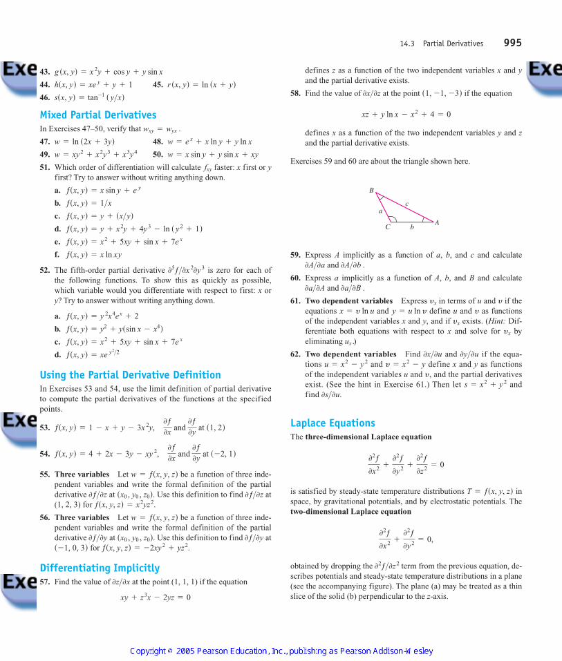
Exercises 59 and 60 are about the triangle shown here.
59. Express A implicitly as a function of a, b, and c and calculateand
60. Express a implicitly as a function of A, b, and B and calculateand
61. Two dependent variables Express in terms of u and y if theequations and define u and y as functionsof the independent variables x and y, and if exists. (Hint: Dif-ferentiate both equations with respect to x and solve for byeliminating
62. Two dependent variables Find and if the equa-tions and define x and y as functionsof the independent variables u and y, and the partial derivativesexist. (See the hint in Exercise 61.) Then let andfind
Laplace EquationsThe three-dimensional Laplace equation
is satisfied by steady-state temperature distributions inspace, by gravitational potentials, and by electrostatic potentials. Thetwo-dimensional Laplace equation
obtained by dropping the term from the previous equation, de-scribes potentials and steady-state temperature distributions in a plane(see the accompanying figure). The plane (a) may be treated as a thinslice of the solid (b) perpendicular to the z-axis.
02ƒ>0z2
02ƒ
0x2 +
02ƒ
0y2 = 0,
T = ƒsx, y, zd
02ƒ
0x2 +
02ƒ
0y2 +
02ƒ
0z2 = 0
0s>0u.s = x2
+ y2
y = x2- yu = x2
- y20y>0u0x>0u
ux .)yx
yx
y = u ln yx = y ln uyx
0a>0B .0a>0A
0A>0b .0A>0a
c
B
CA
a
b
xz + y ln x - x2+ 4 = 0
s1, -1, -3d0x>0z
14.3 Partial Derivatives 995
4100 AWL/Thomas_ch14p965-1066 8/25/04 2:53 PM Page 995
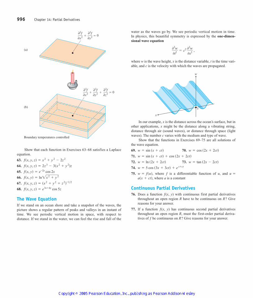
Show that each function in Exercises 63–68 satisfies a Laplaceequation.
63.
64.
65.
66.
67.
68.
The Wave EquationIf we stand on an ocean shore and take a snapshot of the waves, thepicture shows a regular pattern of peaks and valleys in an instant oftime. We see periodic vertical motion in space, with respect todistance. If we stand in the water, we can feel the rise and fall of the
ƒsx, y, zd = e3x + 4y cos 5z
ƒsx, y, zd = sx 2+ y 2
+ z 2d-1>2ƒsx, yd = ln2x 2
+ y 2
ƒsx, yd = e-2y cos 2x
ƒsx, y, zd = 2z 3- 3sx 2
+ y 2dzƒsx, y, zd = x 2
+ y 2- 2z 2
(a)
(b)
Boundary temperatures controlled
� � 0∂2f
∂x2
∂2f
∂y2
� � � 0∂2f
∂x2
∂2f
∂y2
∂2f
∂z2
water as the waves go by. We see periodic vertical motion in time.In physics, this beautiful symmetry is expressed by the one-dimen-sional wave equation
where w is the wave height, x is the distance variable, t is the time vari-able, and c is the velocity with which the waves are propagated.
In our example, x is the distance across the ocean’s surface, but inother applications, x might be the distance along a vibrating string,distance through air (sound waves), or distance through space (lightwaves). The number c varies with the medium and type of wave.
Show that the functions in Exercises 69–75 are all solutions ofthe wave equation.
69. 70.
71.
72. 73.
74.
75. where ƒ is a differentiable function of u, and where a is a constant
Continuous Partial Derivatives76. Does a function ƒ(x, y) with continuous first partial derivatives
throughout an open region R have to be continuous on R? Givereasons for your answer.
77. If a function ƒ(x, y) has continuous second partial derivativesthroughout an open region R, must the first-order partial deriva-tives of ƒ be continuous on R? Give reasons for your answer.
asx + ctd,u =w = ƒsud,
w = 5 cos s3x + 3ctd + e x + ct
w = tan s2x - 2ctdw = ln s2x + 2ctdw = sin sx + ctd + cos s2x + 2ctd
w = cos s2x + 2ctdw = sin sx + ctd
w
x
x
02w
0t2= c2
02w
0x2 ,
996 Chapter 14: Partial Derivatives
4100 AWL/Thomas_ch14p965-1066 8/25/04 2:53 PM Page 996
996 Chapter 14: Partial Derivatives
The Chain Rule
The Chain Rule for functions of a single variable studied in Section 3.5 said that whenwas a differentiable function of x and was a differentiable function of t,
w became a differentiable function of t and dw dt could be calculated with the formula
dwdt
=
dwdx
dxdt
.
> x = gstdw = ƒsxd
14.4
4100 AWL/Thomas_ch14p965-1066 8/25/04 2:53 PM Page 996
For functions of two or more variables the Chain Rule has several forms. The formdepends on how many variables are involved but works like the Chain Rule in Section 3.5once we account for the presence of additional variables.
Functions of Two Variables
The Chain Rule formula for a function when and are bothdifferentiable functions of t is given in the following theorem.
y = ystdx = xstdw = ƒsx, yd
14.4 The Chain Rule 997
THEOREM 5 Chain Rule for Functions of Two Independent VariablesIf has continuous partial derivatives and and ifare differentiable functions of t, then the composite is a differ-entiable function of t and
or
dwdt
=
0ƒ0x
dxdt
+
0ƒ0y
dydt
.
dƒdt
= ƒxsxstd, ystdd # x¿std + ƒysxstd, ystdd # y¿std,
w = ƒsxstd, ystddx = xstd, y = ystdƒyƒxw = ƒsx, yd
Proof The proof consists of showing that if x and y are differentiable at then w isdifferentiable at and
where The subscripts indicate where each of the derivatives are to beevaluated.
Let and be the increments that result from changing t from to Since ƒ is differentiable (see the definition in Section 14.3),
where as To find dw dt, we divide this equation through by and let approach zero. The division gives
Letting approach zero gives
The tree diagram in the margin provides a convenient way to remember the ChainRule. From the diagram, you see that when the derivatives dx dt and dy dt are>>t = t0 ,
= a0w0x bP0
adxdtb
t0
+ a0w0y bP0
adydtb
t0
+ 0 # adxdtb
t0
+ 0 # adydtb
t0
.
adwdtb
t0
= lim¢t:0
¢w¢t
¢t
¢w¢t
= a0w0x bP0
¢x¢t
+ a0w0y bP0
¢y
¢t+ P1
¢x¢t
+ P2 ¢y
¢t.
¢t¢t>¢x, ¢y : 0.P1, P2 : 0
¢w = a0w0x bP0
¢x + a0w0y bP0
¢y + P1¢x + P2¢y ,
t0 + ¢t.t0¢w¢x, ¢y,
P0 = sxst0d, yst0dd.
adwdtb
t0
= a0w0x bP0
adxdtb
t0
+ a0w0y bP0
adydtb
t0
,
t0t = t0 ,
To remember the Chain Rule picture thediagram below. To find dw dt, start at wand read down each route to t,multiplying derivatives along the way.Then add the products.
Chain Rule
t
yx
w � f (x, y)
0w0y
0w0x
dydt
dxdt
dwdt
0w0x
dxdt
0w0y
dydt
� �
Intermediatevariables
Dependentvariable
Independentvariable
>
4100 AWL/Thomas_ch14p965-1066 8/25/04 2:53 PM Page 997
evaluated at The value of then determines the value for the differentiable function xand the value for the differentiable function y. The partial derivatives and (which are themselves functions of x and y) are evaluated at the point correspon-ding to The “true” independent variable is t, whereas x and y are intermediate variables(controlled by t) and w is the dependent variable.
A more precise notation for the Chain Rule shows how the various derivatives in The-orem 5 are evaluated:
EXAMPLE 1 Applying the Chain Rule
Use the Chain Rule to find the derivative of
with respect to t along the path What is the derivative’s value at
Solution We apply the Chain Rule to find dw dt as follows:
In this example, we can check the result with a more direct calculation. As afunction of t,
so
In either case, at the given value of t,
Functions of Three Variables
You can probably predict the Chain Rule for functions of three variables, as it only in-volves adding the expected third term to the two-variable formula.
adwdtb
t =p>2 = cos a2 # p2b = cos p = -1 .
dwdt
=
ddt
a12
sin 2tb =12
# 2 cos 2t = cos 2t .
w = xy = cos t sin t =12
sin 2t ,
= cos 2t.
= -sin2 t + cos2 t
= ssin tds -sin td + scos tdscos td
= s yds -sin td + sxdscos td
=
0sxyd0x #
ddt
scos td +
0sxyd0y #
ddt
ssin td
dwdt
=
0w0x
dxdt
+
0w0y
dydt
>t = p>2?
x = cos t, y = sin t.
w = xy
dwdt
st0d =
0ƒ0x sx0 , y0d # dx
dt st0d +
0ƒ0y sx0 , y0d #
dydt
st0d.
t0.P0sx0, y0d
0w>0y0w>0xy0
x0t0t0.
998 Chapter 14: Partial Derivatives
4100 AWL/Thomas_ch14p965-1066 8/25/04 2:53 PM Page 998
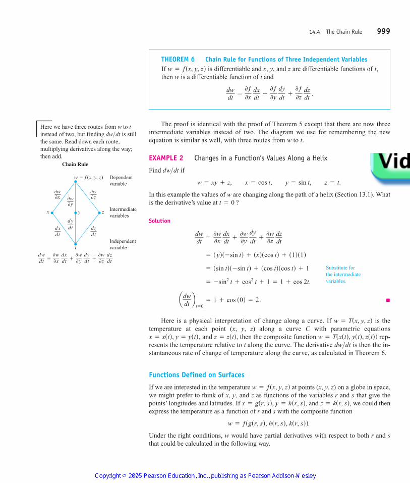
Chain Rule
t
zyx
w � f (x, y, z)
0w0z
0w0x
0w0y
dydt dz
dtdxdt
dwdt
0w0x
dxdt
0w0y
dydt� �
0w0z
dzdt�
Intermediatevariables
Dependentvariable
Independentvariable
The proof is identical with the proof of Theorem 5 except that there are now threeintermediate variables instead of two. The diagram we use for remembering the newequation is similar as well, with three routes from w to t.
EXAMPLE 2 Changes in a Function’s Values Along a Helix
Find dw dt if
In this example the values of w are changing along the path of a helix (Section 13.1). Whatis the derivative’s value at
Solution
Here is a physical interpretation of change along a curve. If is thetemperature at each point (x, y, z) along a curve C with parametric equations
and then the composite function rep-resents the temperature relative to t along the curve. The derivative dw dt is then the in-stantaneous rate of change of temperature along the curve, as calculated in Theorem 6.
Functions Defined on Surfaces
If we are interested in the temperature at points (x, y, z) on a globe in space,we might prefer to think of x, y, and z as functions of the variables r and s that give thepoints’ longitudes and latitudes. If and we could thenexpress the temperature as a function of r and s with the composite function
Under the right conditions, w would have partial derivatives with respect to both r and sthat could be calculated in the following way.
w = ƒsgsr, sd, hsr, sd, ksr, sdd.
z = ksr, sd,x = gsr, sd, y = hsr, sd,
w = ƒsx, y, zd
>w = Tsxstd, ystd, zstddz = zstd,x = xstd, y = ystd,
w = Tsx, y, zd
adwdtb
t = 0= 1 + cos s0d = 2.
= -sin2 t + cos2 t + 1 = 1 + cos 2t.
= ssin tds -sin td + scos tdscos td + 1
= s yds -sin td + sxdscos td + s1ds1d
dwdt
=
0w0x
dxdt
+
0w0y
dydt
+
0w0z
dzdt
t = 0 ?
w = xy + z, x = cos t, y = sin t, z = t.
>
14.4 The Chain Rule 999
Here we have three routes from w to tinstead of two, but finding dw dt is stillthe same. Read down each route,multiplying derivatives along the way;then add.
>
THEOREM 6 Chain Rule for Functions of Three Independent VariablesIf is differentiable and x, y, and z are differentiable functions of t,then w is a differentiable function of t and
dwdt
=
0ƒ0x
dxdt
+
0ƒ0y
dydt
+
0ƒ0z
dzdt
.
w = ƒsx, y, zd
Substitute forthe intermediatevariables.
4100 AWL/Thomas_ch14p965-1066 8/25/04 2:53 PM Page 999
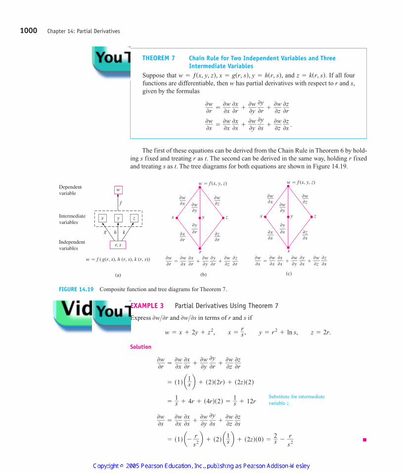
The first of these equations can be derived from the Chain Rule in Theorem 6 by hold-ing s fixed and treating r as t. The second can be derived in the same way, holding r fixedand treating s as t. The tree diagrams for both equations are shown in Figure 14.19.
1000 Chapter 14: Partial Derivatives
THEOREM 7 Chain Rule for Two Independent Variables and ThreeIntermediate Variables
Suppose that and If all fourfunctions are differentiable, then w has partial derivatives with respect to r and s,given by the formulas
0w0s =
0w0x
0x0s +
0w0y
0y0s +
0w0z
0z0s .
0w0r =
0w0x
0x0r +
0w0y
0y0r +
0w0z
0z0r
z = ksr, sd.w = ƒsx, y, zd, x = gsr, sd, y = hsr, sd,
w
(a)
g h k
f
x y z
r, s
Dependentvariable
Independentvariables
Intermediatevariables
w � f ( g(r, s), h (r, s), k (r, s))
(b)
r
zx y
w � f (x, y, z)
0w0x 0w
0y
0y0r
0x0r
0w0z
0z0r
0w0r
0w0x
0x0r
0w0y
0y0r�
0w0z
0z0r��
s
zx y
(c)
0w0x
0w0y
0y0s0x
0s
0w0z
0z0s
0w0s
0w0x
0x0s
0w0y
0y0s�
0w0z
0z0s��
w � f (x, y, z)
FIGURE 14.19 Composite function and tree diagrams for Theorem 7.
EXAMPLE 3 Partial Derivatives Using Theorem 7
Express and in terms of r and s if
Solution
= s1d a- rs2 b + s2d a1s b + s2zds0d =
2s -
rs2
0w0s =
0w0x
0x0s +
0w0y
0y0s +
0w0z
0z0s
=1s + 4r + s4rds2d =
1s + 12r
= s1d a1s b + s2ds2rd + s2zds2d
0w0r =
0w0x
0x0r +
0w0y
0y0r +
0w0z
0z0r
w = x + 2y + z2, x =rs , y = r2
+ ln s, z = 2r.
0w>0s0w>0r
Substitute for intermediatevariable z.
4100 AWL/Thomas_ch14p965-1066 8/25/04 2:53 PM Page 1000
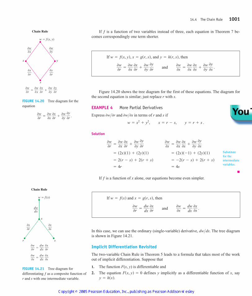
If ƒ is a function of two variables instead of three, each equation in Theorem 7 be-comes correspondingly one term shorter.
14.4 The Chain Rule 1001
If and then
0w0r =
0w0x
0x0r +
0w0y
0y0r and 0w
0s =
0w0x
0x0s +
0w0y
0y0s .
y = hsr, sd,w = ƒsx, yd, x = gsr, sd,
Chain Rule
r
yx
w � f (x, y)
0w0x
0x0r
0w0y
0y0r
0w0r
0w0x
0x0r
0w0y
0y0r� �
FIGURE 14.20 Tree diagram for theequation
0w0r =
0w0x
0x0r +
0w0y
0y0r .
Figure 14.20 shows the tree diagram for the first of these equations. The diagram forthe second equation is similar; just replace r with s.
EXAMPLE 4 More Partial Derivatives
Express and in terms of r and s if
Solution
If ƒ is a function of x alone, our equations become even simpler.
= 4r = 4s
= 2sr - sd + 2sr + sd = -2sr - sd + 2sr + sd
= s2xds1d + s2yds1d = s2xds -1d + s2yds1d
0w0r =
0w0x
0x0r +
0w0y
0y0r
0w0s =
0w0x
0x0s +
0w0y
0y0s
w = x2+ y2, x = r - s, y = r + s .
0w>0s0w>0r
Substitutefor theintermediatevariables.
If and then
0w0r =
dwdx
0x0r and 0w
0s =
dwdx
0x0s .
x = gsr, sd,w = ƒsxd
Chain Rule
r
x
s
w � f (x)
dwdx
0x0r
0x0s
0w0r
dwdx
0x0r�
0w0s
dwdx
0x0s�
FIGURE 14.21 Tree diagram fordifferentiating ƒ as a composite function ofr and s with one intermediate variable.
In this case, we can use the ordinary (single-variable) derivative, dw dx. The tree diagramis shown in Figure 14.21.
Implicit Differentiation Revisited
The two-variable Chain Rule in Theorem 5 leads to a formula that takes most of the workout of implicit differentiation. Suppose that
1. The function F(x, y) is differentiable and
2. The equation defines y implicitly as a differentiable function of x, sayy = hsxd.
Fsx, yd = 0
>
4100 AWL/Thomas_ch14p965-1066 8/25/04 2:53 PM Page 1001
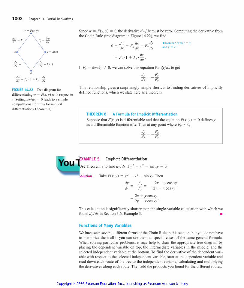
Since the derivative dw dx must be zero. Computing the derivative fromthe Chain Rule (tree diagram in Figure 14.22), we find
If we can solve this equation for dy dx to get
This relationship gives a surprisingly simple shortcut to finding derivatives of implicitlydefined functions, which we state here as a theorem.
dydx
= -
Fx
Fy.
>Fy = 0w>0y Z 0,
= Fx# 1 + Fy
#dydx
.
0 =
dwdx
= Fx dxdx
+ Fy dydx
>w = Fsx, yd = 0,
1002 Chapter 14: Partial Derivatives
Theorem 5 withand ƒ = F
t = x
x
x
w � F(x, y)
� Fx0w0x
dxdx � 1
y � h(x)
Fy �0w0y
dydx � h'(x)
� Fx • 1 � Fy •dwdx
dydx
FIGURE 14.22 Tree diagram fordifferentiating with respect tox. Setting leads to a simplecomputational formula for implicitdifferentiation (Theorem 8).
dw>dx = 0w = Fsx, yd
THEOREM 8 A Formula for Implicit DifferentiationSuppose that F(x, y) is differentiable and that the equation defines yas a differentiable function of x. Then at any point where
dydx
= -
Fx
Fy.
Fy Z 0,Fsx, yd = 0
EXAMPLE 5 Implicit Differentiation
Use Theorem 8 to find dy dx if
Solution Take Then
This calculation is significantly shorter than the single-variable calculation with which wefound dy dx in Section 3.6, Example 3.
Functions of Many Variables
We have seen several different forms of the Chain Rule in this section, but you do not haveto memorize them all if you can see them as special cases of the same general formula.When solving particular problems, it may help to draw the appropriate tree diagram byplacing the dependent variable on top, the intermediate variables in the middle, and theselected independent variable at the bottom. To find the derivative of the dependent vari-able with respect to the selected independent variable, start at the dependent variable andread down each route of the tree to the independent variable, calculating and multiplyingthe derivatives along each route. Then add the products you found for the different routes.
>
=
2x + y cos xy2y - x cos xy
.
dydx
= -
Fx
Fy= -
-2x - y cos xy2y - x cos xy
Fsx, yd = y 2- x 2
- sin xy.
y 2- x 2
- sin xy = 0.>
4100 AWL/Thomas_ch14p965-1066 8/25/04 2:53 PM Page 1002

In general, suppose that is a differentiable function of the vari-ables (a finite set) and the are differentiable functions of
(another finite set). Then w is a differentiable function of the variables pthrough t and the partial derivatives of w with respect to these variables are given byequations of the form
The other equations are obtained by replacing p by one at a time.One way to remember this equation is to think of the right-hand side as the dot
product of two vectors with components
Derivatives of w with Derivatives of the intermediaterespect to the variables with respect to the
intermediate variables selected independent variable
('''')''''*('''')''''*
a0w0x ,
0w0y , Á ,
0w0yb and a0x
0p, 0y0p, Á ,
0y0p b .
q, Á , t,
0w0p =
0w0x
0x0p +
0w0y
0y0p +
Á+
0w0y
0y0p .
p, q, Á , tx, y, Á , yx, y, Á , y
w = ƒsx, y, Á , yd
14.4 The Chain Rule 1003
4100 AWL/Thomas_ch14p965-1066 8/25/04 2:53 PM Page 1003
14.4 The Chain Rule 1003
EXERCISES 14.4
Chain Rule: One Independent VariableIn Exercises 1–6, (a) express dw dt as a function of t, both by usingthe Chain Rule and by expressing w in terms of t and differentiatingdirectly with respect to t. Then (b) evaluate dw dt at the given valueof t.
1.
2.
3.
4.
5.
6.
Chain Rule: Two and Three Independent VariablesIn Exercises 7 and 8, (a) express and as functions of u and
both by using the Chain Rule and by expressing z directly in termsof u and before differentiating. Then (b) evaluate and atthe given point
7.
8.
In Exercises 9 and 10, (a) express and as functions of uand y both by using the Chain Rule and by expressing w directly in
0w>0y0w>0u
su, yd = s1.3, p>6dz = tan-1 sx>yd, x = u cos y, y = u sin y; su, yd = s2, p>4dz = 4e x ln y, x = ln su cos yd, y = u sin y;
su, yd.0z>0y0z>0uy
y
0z>0y0z>0u
w = z - sin xy, x = t, y = ln t, z = et - 1 ; t = 1
t = 1w = 2ye x
- ln z, x = ln st 2+ 1d, y = tan-1 t, z = e t;
t = 3w = ln sx 2
+ y 2+ z 2d, x = cos t, y = sin t, z = 42t ;
w =
xz +
yz , x = cos2 t, y = sin2 t, z = 1>t; t = 3
w = x 2+ y 2, x = cos t + sin t, y = cos t - sin t; t = 0
w = x 2+ y 2, x = cos t, y = sin t; t = p
>>
terms of u and y before differentiating. Then (b) evaluate andat the given point (u, y).
9.
10.
In Exercises 11 and 12, (a) express and as functionsof x, y, and z both by using the Chain Rule and by expressing u di-rectly in terms of x, y, and z before differentiating. Then (b) evaluate
and at the given point (x, y, z).
11.
12.
Using a Tree DiagramIn Exercises 13–24, draw a tree diagram and write a Chain Rule for-mula for each derivative.
13.
14.
15.
z = ksu, yd
0w0u and
0w0y
for w = hsx, y, zd, x = ƒsu, yd, y = gsu, yd,
dzdt
for z = ƒsu, y, wd, u = gstd, y = hstd, w = kstd
dzdt
for z = ƒsx, yd, x = gstd, y = hstd
sx, y, zd = sp>4, 1>2, -1>2du = e qr sin-1 p, p = sin x, q = z 2 ln y, r = 1>z;
sx, y, zd = A23, 2, 1 Br = x + y - z;
u =
p - qq - r , p = x + y + z, q = x - y + z,
0u>0z0u>0x, 0u>0y,
0u>0z0u>0x, 0u>0y,
z = uey; su, yd = s -2, 0dw = ln sx 2
+ y 2+ z 2d, x = uey sin u, y = uey cos u,
su, yd = s1>2, 1dw = xy + yz + xz, x = u + y, y = u - y, z = uy;
0w>0y 0w>0u
4100 AWL/Thomas_ch14p965-1066 8/25/04 2:53 PM Page 1003
16.
17.
18.
19.
20.
21.
22.
23.
24.
Implicit DifferentiationAssuming that the equations in Exercises 25–28 define y as a differen-tiable function of x, use Theorem 8 to find the value of dy dx at thegiven point.
25.
26.
27.
28.
Three-Variable Implicit DifferentiationTheorem 8 can be generalized to functions of three variables and evenmore. The three-variable version goes like this: If the equation
determines z as a differentiable function of x and y,then, at points where
Use these equations to find the values of and at thepoints in Exercises 29–32.
29.
30.
31.
32. xe y+ ye z
+ 2 ln x - 2 - 3 ln 2 = 0, s1, ln 2, ln 3dsin sx + yd + sin s y + zd + sin sx + zd = 0, sp, p, pd
1x +
1y +
1z - 1 = 0, s2, 3, 6d
z3- xy + yz + y 3
- 2 = 0, s1, 1, 1d
0z>0y0z>0x
0z0x = -
Fx
Fz and 0z
0y = -
Fy
Fz.
Fz Z 0,Fsx, y, zd = 0
xe y+ sin xy + y - ln 2 = 0, s0, ln 2d
x2+ xy + y 2
- 7 = 0, s1, 2dxy + y 2
- 3x - 3 = 0, s -1, 1dx 3
- 2y 2+ xy = 0, s1, 1d
>
0w0s for w = gsx, yd, x = hsr, s, td, y = ksr, s, td
0w0r and
0w0s for w = ƒsx, yd, x = gsrd, y = hssd
z = js p, qd, y = ks p, qd
0w0p for w = ƒsx, y, z, yd, x = gs p, qd, y = hs p, qd,
0w0s and
0w0t for w = gsud, u = hss, td
0y0r for y = ƒsud, u = gsr, sd
0z0t and
0z0s for z = ƒsx, yd, x = gst, sd, y = hst, sd
0w0x and
0w0y for w = gsu, yd, u = hsx, yd, y = ksx, yd
0w0u and
0w0y
for w = gsx, yd, x = hsu, yd, y = ksu, yd
t = ksx, yd
0w0x and
0w0y for w = ƒsr, s, td, r = gsx, yd, s = hsx, yd, Finding Specified Partial Derivatives
33. Find when if
34. Find when if
35. Find when if
36. Find when if
37. Find and when if and
38. Find and when and if and
Theory and Examples39. Changing voltage in a circuit The voltage V in a circuit that
satisfies the law is slowly dropping as the battery wearsout. At the same time, the resistance R is increasing as the resistorheats up. Use the equation
to find how the current is changing at the instant when and
40. Changing dimensions in a box The lengths a, b, and c of the edgesof a rectangular box are changing with time. At the instant in ques-tion, and At what rates are the box’s volume V andsurface area S changing at that instant? Are the box’s interior di-agonals increasing in length or decreasing?
41. If ƒ(u, y, w) is differentiable and andshow that
42. Polar coordinates Suppose that we substitute polar coordinatesand in a differentiable function
w = ƒsx, yd.y = r sin ux = r cos u
0ƒ0x +
0ƒ0y +
0ƒ0z = 0.
w = z - x,u = x - y, y = y - z,
dc>dt = -3 m>sec.da>dt = db>dt = 1 m>sec,c = 3 m,b = 2 m,a = 1 m,
R
� �V
I
Battery
-0.01 volt>sec.dV>dt =dR>dt = 0.5 ohm>sec,I = 0.04 amp,600 ohms,
R =
dVdt
=
0V0I
dIdt
+
0V0R
dRdt
V = IR
q = 1y + 3 tan-1 u.z = ln qy = -2u = 10z>0y0z>0u
x = eu+ ln y.
z = 5 tan-1 xu = ln 2, y = 10z>0y0z>0u
x = u2+ y2, y = uy.
z = sin xy + x sin y,u = 0, y = 10z>0u
x = u - 2y + 1, y = 2u + y - 2.w = x2
+ sy>xd,u = 0, y = 00w>0yx = y2>u, y = u + y, z = cos u.
w = xy + ln z,u = -1, y = 20w>0yy = cos sr + sd, z = sin sr + sd.x = r - s,
w = sx + y + zd2, r = 1, s = -10w>0r
1004 Chapter 14: Partial Derivatives
4100 AWL/Thomas_ch14p965-1066 8/25/04 2:53 PM Page 1004
a. Show that
and
b. Solve the equations in part (a) to express and in terms ofand
c. Show that
43. Laplace equations Show that if satisfies theLaplace equation and if and
then w satisfies the Laplace equation
44. Laplace equations Let where
and and Show that w satisfies the Laplaceequation if all the necessary functions are differ-entiable.
Changes in Functions Along Curves45. Extreme values on a helix Suppose that the partial derivatives
of a function ƒ(x, y, z) at points on the helix are
At what points on the curve, if any, can ƒ take on extreme values?
46. A space curve Let Find the value of dw dt atthe point (1, ln 2, 0) on the curve
47. Temperature on a circle Let be the temperature atthe point (x, y) on the circle and suppose that
a. Find where the maximum and minimum temperatures on thecircle occur by examining the derivatives dT dt and d 2T>dt 2.>
0T0x = 8x - 4y, 0T
0y = 8y - 4x.
x = cos t, y = sin t, 0 … t … 2pT = ƒsx, yd
z = t .x = cos t, y = ln st + 2d,>w = x 2e 2y cos 3z .
ƒx = cos t, ƒy = sin t, ƒz = t 2+ t - 2.
z = tx = cos t, y = sin t,
wxx + wyy = 0i = 2-1.y = x - iy
u = x + iyw = ƒsud + g syd,wxx + wyy = 0.y = xy,
u = sx 2- y 2d>2ƒuu + ƒyy = 0
w = ƒsu, yd
sƒxd2+ sƒyd2
= a0w0r b
2
+
1r 2 a0w
0ub2
.
0w>0u.0w>0rƒyƒx
1r
0w0u
= -ƒx sin u + ƒy cos u .
0w0r = ƒx cos u + ƒy sin u
b. Suppose that Find the maximum andminimum values of T on the circle.
48. Temperature on an ellipse Let be the temperatureat the point (x, y) on the ellipse
and suppose that
a. Locate the maximum and minimum temperatures on theellipse by examining dT dt and
b. Suppose that Find the maximum and minimumvalues of T on the ellipse.
Differentiating IntegralsUnder mild continuity restrictions, it is true that if
then Using this fact and the Chain Rule, we
can find the derivative of
by letting
where Find the derivatives of the functions in Exercises 49and 50.
49.
50. Fsxd = L1
x22t 3
+ x 2 dt
Fsxd = Lx2
02t 4
+ x 3 dt
u = ƒsxd.
Gsu, xd = Lu
a g st, xd dt,
Fsxd = Lƒsxd
a g st, xd dt
F¿sxd = Lb
a gxst, xd dt.
Fsxd = Lb
a g st, xd dt,
T = xy - 2.
d2T>dt2.>
0T0x = y, 0T
0y = x.
x = 222 cos t, y = 22 sin t, 0 … t … 2p,
T = g sx, yd
T = 4x 2- 4xy + 4y 2.
1005
4100 AWL/Thomas_ch14p965-1066 8/25/04 2:53 PM Page 1005
14.4 The Chain Rule
14.5 Directional Derivatives and Gradient Vectors 1005
Directional Derivatives and Gradient Vectors
If you look at the map (Figure 14.23) showing contours on the West Point Area along theHudson River in New York, you will notice that the tributary streams flow perpendicular tothe contours. The streams are following paths of steepest descent so the waters reach theHudson as quickly as possible. Therefore, the instantaneous rate of change in a stream’s
14.5
4100 AWL/Thomas_ch14p965-1066 8/25/04 2:53 PM Page 1005
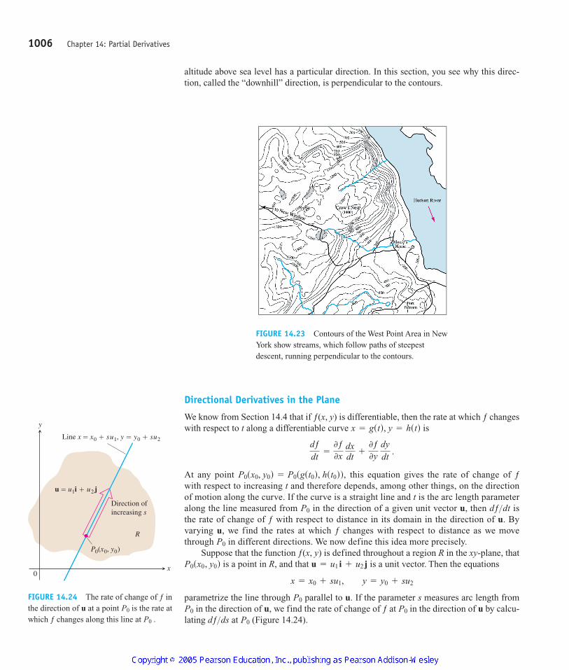
Directional Derivatives in the Plane
We know from Section 14.4 that if ƒ(x, y) is differentiable, then the rate at which ƒ changeswith respect to t along a differentiable curve is
At any point this equation gives the rate of change of ƒwith respect to increasing t and therefore depends, among other things, on the directionof motion along the curve. If the curve is a straight line and t is the arc length parameteralong the line measured from in the direction of a given unit vector u, then dƒ dt isthe rate of change of ƒ with respect to distance in its domain in the direction of u. Byvarying u, we find the rates at which ƒ changes with respect to distance as we movethrough in different directions. We now define this idea more precisely.
Suppose that the function ƒ(x, y) is defined throughout a region R in the xy-plane, thatis a point in R, and that is a unit vector. Then the equations
parametrize the line through parallel to u. If the parameter s measures arc length fromin the direction of u, we find the rate of change of ƒ at in the direction of u by calcu-
lating dƒ ds at (Figure 14.24).P0>P0P0
P0
x = x0 + su1, y = y0 + su2
u = u1 i + u2 jP0sx0, y0d
P0
>P0
P0sx0, y0d = P0sgst0d, hst0dd,
dƒdt
=
0ƒ0x
dxdt
+
0ƒ0y
dydt
.
x = gstd, y = hstd
1006 Chapter 14: Partial Derivatives
FIGURE 14.23 Contours of the West Point Area in NewYork show streams, which follow paths of steepestdescent, running perpendicular to the contours.
x
y
0
R
Line x � x0 � su1, y � y0 � su2
u � u1i � u2 j
Direction ofincreasing s
P0(x0, y0)
FIGURE 14.24 The rate of change of ƒ inthe direction of u at a point is the rate atwhich ƒ changes along this line at P0 .
P0
altitude above sea level has a particular direction. In this section, you see why this direc-tion, called the “downhill” direction, is perpendicular to the contours.
4100 AWL/Thomas_ch14p965-1066 8/25/04 2:53 PM Page 1006
The directional derivative is also denoted by
EXAMPLE 1 Finding a Directional Derivative Using the Definition
Find the derivative of
at in the direction of the unit vector
Solution
The rate of change of at in the direction
is
Interpretation of the Directional Derivative
The equation represents a surface S in space. If then the pointlies on S. The vertical plane that passes through P and parallel to uP0sx0, y0dPsx0, y0, z0d
z0 = ƒsx0, y0d,z = ƒsx, yd
5>12.A1>22 B ju = A1>12 B i +P0s1, 2dƒsx, yd = x2
+ xy
= lims:0
5s22+ s2
s = lims:0
¢ 522+ s≤ = ¢ 522
+ 0≤ =
522.
= lims:0
¢1 +
2s22+
s2
2 ≤ + ¢2 +
3s22+
s2
2 ≤ - 3
s
= lims:0
¢1 +
s22≤2
+ ¢1 +
s22≤ ¢2 +
s22≤ - s12
+ 1 # 2d
s
= lims:0
Ģ1 + s # 122, 2 + s # 122
≤ - ƒs1, 2d
s
¢dƒds≤
u,P0
= lims:0
ƒsx0 + su1, y0 + su2d - ƒsx0, y0d
s
u = A1>22 B i + A1>22 B j.P0s1, 2d
ƒsx, yd = x 2+ xy
sDu ƒdP0.
14.5 Directional Derivatives and Gradient Vectors 1007
DEFINITION Directional DerivativeThe derivative of ƒ at in the direction of the unit vector
is the number
(1)
provided the limit exists.
adƒdsb
u,P0
= lims:0
ƒsx0 + su1, y0 + su2d - ƒsx0, y0d
s ,
u2ju � u1i �P0(x0, y0)
“The derivative of ƒ at in the direction of u”
P0
Equation (1)
4100 AWL/Thomas_ch14p965-1066 8/25/04 2:53 PM Page 1007
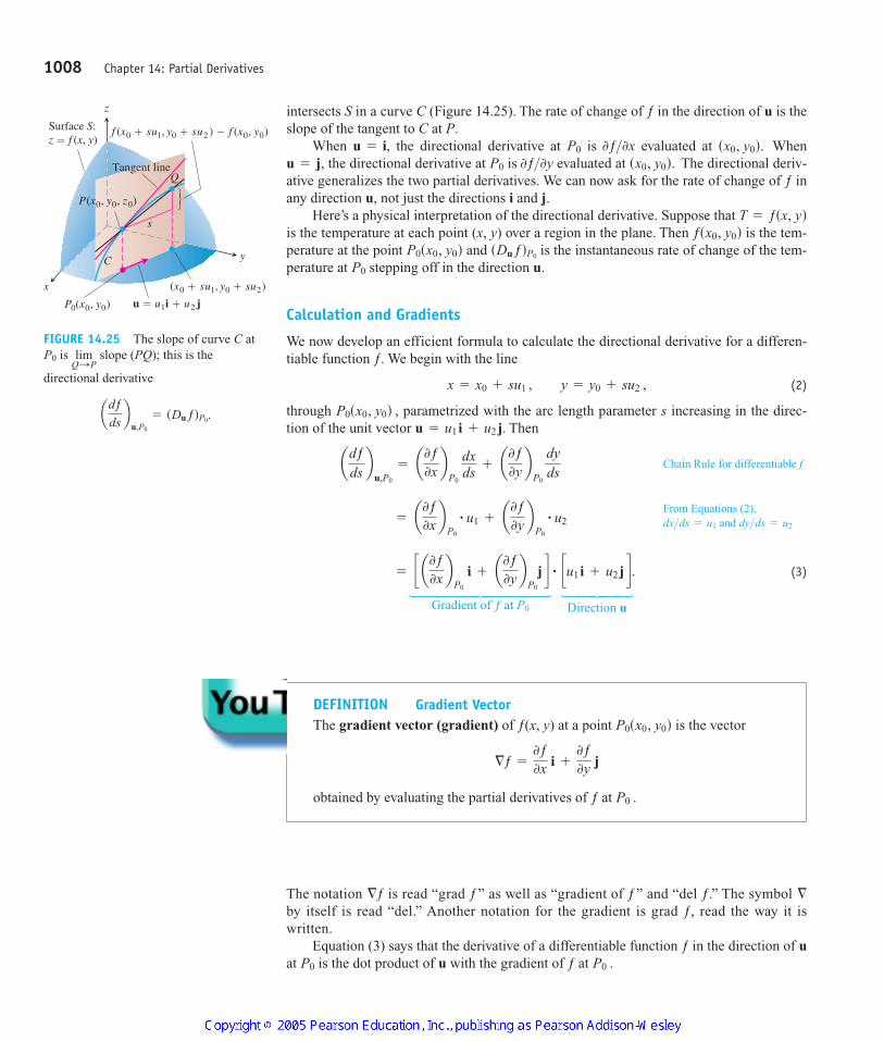
intersects S in a curve C (Figure 14.25). The rate of change of ƒ in the direction of u is theslope of the tangent to C at P.
When the directional derivative at is evaluated at Whenthe directional derivative at is evaluated at The directional deriv-
ative generalizes the two partial derivatives. We can now ask for the rate of change of ƒ inany direction u, not just the directions i and j.
Here’s a physical interpretation of the directional derivative. Suppose that is the temperature at each point (x, y) over a region in the plane. Then is the tem-perature at the point and is the instantaneous rate of change of the tem-perature at stepping off in the direction u.
Calculation and Gradients
We now develop an efficient formula to calculate the directional derivative for a differen-tiable function ƒ. We begin with the line
(2)
through parametrized with the arc length parameter s increasing in the direc-tion of the unit vector Then
(3)
Direction uGradient of ƒ at P0
('')''*(''''')'''''*
= c a0ƒ0x bP0
i + a0ƒ0y bP0
j d # cu1 i + u2 j d .
= a0ƒ0x bP0
# u1 + a0ƒ0y bP0
# u2
adƒdsb
u,P0
= a0ƒ0x bP0
dxds
+ a0ƒ0y bP0
dyds
u = u1 i + u2 j.P0sx0, y0d ,
x = x0 + su1 , y = y0 + su2 ,
P0
sDu ƒdP0P0sx0, y0dƒsx0, y0d
T = ƒsx, yd
sx0, y0d.0ƒ>0yP0u = j,sx0, y0d.0ƒ>0xP0u = i,
1008 Chapter 14: Partial Derivatives
z
x
yC
Q
s
Surface S:z � f (x, y)
f (x0 � su1, y0 � su2 ) � f (x0, y0)
Tangent line
P(x0, y0, z0)
P0(x0, y0) u � u1i � u2 j
(x0 � su1, y0 � su2)
FIGURE 14.25 The slope of curve C atis slope (PQ); this is the
directional derivative
adƒ
dsb
u,P0
= sDu ƒdP0.
limQ:P
P0
Chain Rule for differentiable f
From Equations (2),and dy>ds = u2dx>ds = u1
DEFINITION Gradient VectorThe gradient vector (gradient) of ƒ(x, y) at a point is the vector
obtained by evaluating the partial derivatives of ƒ at P0 .
§ƒ =
0ƒ0x i +
0ƒ0y j
P0sx0, y0d
The notation is read “grad ƒ” as well as “gradient of ƒ” and “del ƒ.” The symbol by itself is read “del.” Another notation for the gradient is grad ƒ, read the way it iswritten.
Equation (3) says that the derivative of a differentiable function ƒ in the direction of uat is the dot product of u with the gradient of ƒ at P0 .P0
§§ƒ
4100 AWL/Thomas_ch14p965-1066 8/25/04 2:53 PM Page 1008
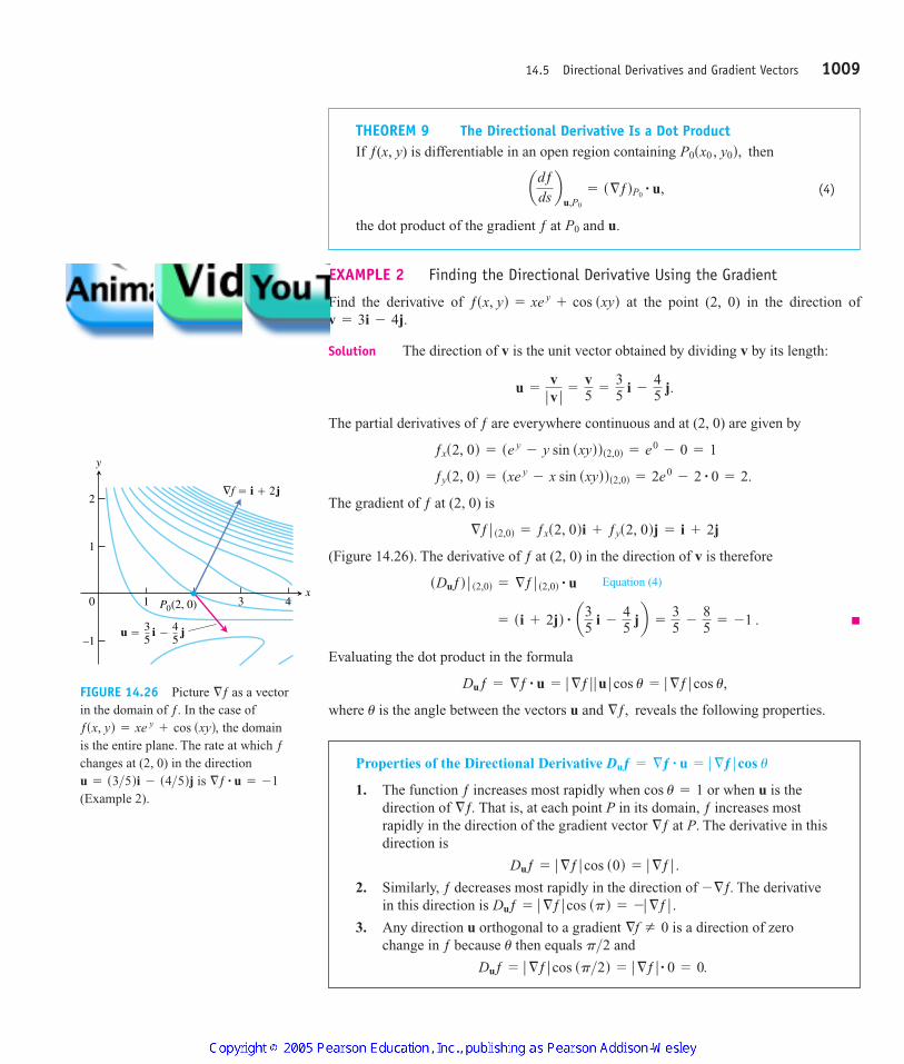
EXAMPLE 2 Finding the Directional Derivative Using the Gradient
Find the derivative of at the point (2, 0) in the direction of
Solution The direction of v is the unit vector obtained by dividing v by its length:
The partial derivatives of ƒ are everywhere continuous and at (2, 0) are given by
The gradient of ƒ at (2, 0) is
(Figure 14.26). The derivative of ƒ at (2, 0) in the direction of v is therefore
Evaluating the dot product in the formula
where is the angle between the vectors u and reveals the following properties.§ƒ,u
Duƒ = §ƒ # u = ƒ §ƒ ƒ ƒ u ƒ cos u = ƒ §ƒ ƒ cos u,
= si + 2jd # a35 i -45 jb =
35 -
85 = -1 .
sDuƒd ƒ s2,0d = §ƒ ƒ s2,0d # u
§ƒ ƒ s2,0d = ƒxs2, 0di + ƒys2, 0dj = i + 2j
ƒys2, 0d = sxe y- x sin sxydds2,0d = 2e0
- 2 # 0 = 2.
ƒxs2, 0d = se y- y sin sxydds2,0d = e0
- 0 = 1
u =
vƒ v ƒ
=
v5 =
35 i -
45 j.
v = 3i - 4j.ƒsx, yd = xe y
+ cos sxyd
14.5 Directional Derivatives and Gradient Vectors 1009
THEOREM 9 The Directional Derivative Is a Dot ProductIf ƒ(x, y) is differentiable in an open region containing then
(4)
the dot product of the gradient ƒ at and u.P0
adƒdsb
u,P0
= s§ƒdP0# u,
P0sx0 , y0d,
Equation (4)x
y
0 1 3 4
–1
1
2∇f � i � 2j
u � i � j35
45
P0(2, 0)
FIGURE 14.26 Picture as a vector in the domain of ƒ. In the case of
the domain is the entire plane. The rate at which ƒchanges at (2, 0) in the direction
is (Example 2).
§ƒ # u = -1u = s3>5di - s4>5dj
ƒsx, yd = xe y+ cos sxyd,
§ƒ
Properties of the Directional Derivative
1. The function ƒ increases most rapidly when or when u is thedirection of That is, at each point P in its domain, ƒ increases mostrapidly in the direction of the gradient vector at P. The derivative in thisdirection is
2. Similarly, ƒ decreases most rapidly in the direction of The derivativein this direction is
3. Any direction u orthogonal to a gradient is a direction of zerochange in ƒ because then equals and
Duƒ = ƒ §ƒ ƒ cos sp>2d = ƒ §ƒ ƒ# 0 = 0.
p>2u
§f Z 0
Duƒ = ƒ §ƒ ƒ cos spd = - ƒ §ƒ ƒ .- §ƒ.
Duƒ = ƒ §ƒ ƒ cos s0d = ƒ §ƒ ƒ .
§ƒ§ƒ.
cos u = 1
Duƒ = §ƒ # u = ƒ §ƒ ƒ cos u
4100 AWL/Thomas_ch14p965-1066 8/25/04 2:53 PM Page 1009
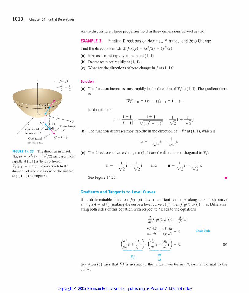
As we discuss later, these properties hold in three dimensions as well as two.
EXAMPLE 3 Finding Directions of Maximal, Minimal, and Zero Change
Find the directions in which
(a) Increases most rapidly at the point (1, 1)
(b) Decreases most rapidly at (1, 1).
(c) What are the directions of zero change in ƒ at (1, 1)?
Solution
(a) The function increases most rapidly in the direction of at (1, 1). The gradient thereis
Its direction is
(b) The function decreases most rapidly in the direction of at (1, 1), which is
(c) The directions of zero change at (1, 1) are the directions orthogonal to
See Figure 14.27.
Gradients and Tangents to Level Curves
If a differentiable function ƒ(x, y) has a constant value c along a smooth curve(making the curve a level curve of ƒ), then Differenti-
ating both sides of this equation with respect to t leads to the equations
(5)
Equation (5) says that is normal to the tangent vector dr dt, so it is normal to thecurve.
>§ƒ
dr
dt§ƒ
('')''*('')''*
a0ƒ0x i +
0ƒ0y jb # adg
dt i +
dhdt
jb = 0.
0ƒ0x
dgdt
+
0ƒ0y
dhdt
= 0
ddt
ƒsgstd, hstdd =
ddt
scd
ƒsgstd, hstdd = c.r = gstdi + hstdj
n = -122
i +122
j and -n =122
i -122
j.
§ƒ:
-u = -122
i -122
j.
- §ƒ
u =
i + j
ƒ i + j ƒ
=
i + j2s1d2+ s1d2
=122
i +122
j.
s§ƒds1,1d = sxi + yjds1,1d = i + j .
§ƒ
ƒsx, yd = sx 2>2d + s y 2>2d
1010 Chapter 14: Partial Derivatives
z
x
y1
1
(1, 1)
(1, 1, 1)
Most rapidincrease in f
Most rapiddecrease in f
∇f � i � j
Zero changein f
–∇f
z � f (x, y)
� �2x2
2y2
FIGURE 14.27 The direction in whichincreases most
rapidly at (1, 1) is the direction ofIt corresponds to the
direction of steepest ascent on the surfaceat (1, 1, 1) (Example 3).
§ƒ ƒ s1,1d = i + j.
ƒsx, yd = sx2>2d + s y2>2d
Chain Rule
4100 AWL/Thomas_ch14p965-1066 8/25/04 2:53 PM Page 1010
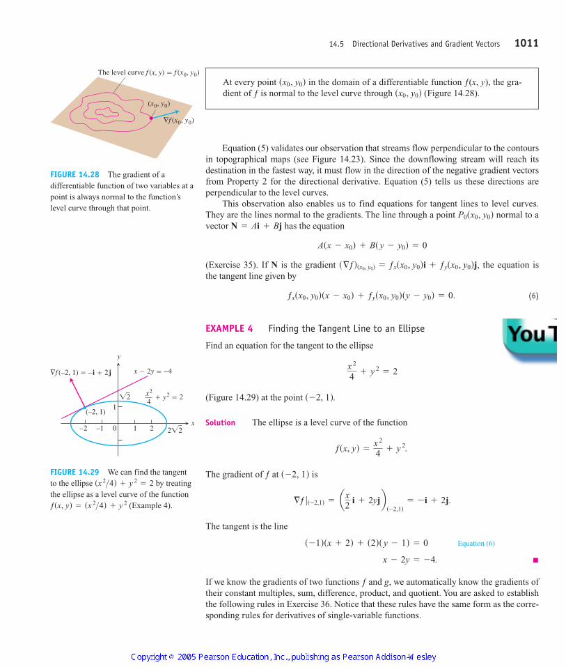
Equation (5) validates our observation that streams flow perpendicular to the contoursin topographical maps (see Figure 14.23). Since the downflowing stream will reach itsdestination in the fastest way, it must flow in the direction of the negative gradient vectorsfrom Property 2 for the directional derivative. Equation (5) tells us these directions areperpendicular to the level curves.
This observation also enables us to find equations for tangent lines to level curves.They are the lines normal to the gradients. The line through a point normal to avector has the equation
(Exercise 35). If N is the gradient the equation isthe tangent line given by
(6)
EXAMPLE 4 Finding the Tangent Line to an Ellipse
Find an equation for the tangent to the ellipse
(Figure 14.29) at the point
Solution The ellipse is a level curve of the function
The gradient of ƒ at is
The tangent is the line
If we know the gradients of two functions ƒ and g, we automatically know the gradients oftheir constant multiples, sum, difference, product, and quotient. You are asked to establishthe following rules in Exercise 36. Notice that these rules have the same form as the corre-sponding rules for derivatives of single-variable functions.
x - 2y = -4.
s -1dsx + 2d + s2ds y - 1d = 0
§ƒ ƒ s-2,1d = ax2
i + 2yjbs-2,1d
= - i + 2j.
s -2, 1d
ƒsx, yd =
x 2
4+ y 2.
s -2, 1d.
x 2
4+ y 2
= 2
ƒxsx0, y0dsx - x0d + ƒysx0, y0dsy - y0d = 0.
s§ƒdsx0, y0d = ƒxsx0, y0di + ƒysx0, y0dj,
Asx - x0d + Bs y - y0d = 0
N = Ai + BjP0sx0, y0d
14.5 Directional Derivatives and Gradient Vectors 1011
At every point in the domain of a differentiable function ƒ(x, y), the gra-dient of ƒ is normal to the level curve through (Figure 14.28).sx0, y0d
sx0, y0dThe level curve f (x, y) � f (x0, y0)
(x0, y0)
∇f (x0, y0)
FIGURE 14.28 The gradient of adifferentiable function of two variables at apoint is always normal to the function’slevel curve through that point.
Equation (6)
y
x0–1–2
1
1 2
∇f (–2, 1) � – i � 2j x � 2y � –4
(–2, 1)
�2
2�2
� y2 � 2x2
4
FIGURE 14.29 We can find the tangentto the ellipse by treatingthe ellipse as a level curve of the function
(Example 4).ƒsx, yd = sx 2>4d + y 2
sx 2>4d + y 2= 2
4100 AWL/Thomas_ch14p965-1066 8/25/04 2:53 PM Page 1011
EXAMPLE 5 Illustrating the Gradient Rules
We illustrate the rules with
We have
1.
2.
3.
4.
5.
Functions of Three Variables
For a differentiable function ƒ(x, y, z) and a unit vector in space, wehave
and
Duƒ = §ƒ # u =
0ƒ0x u1 +
0ƒ0y u2 +
0ƒ0z u3.
§ƒ =
0ƒ0x i +
0ƒ0y j +
0ƒ0z k
u = u1 i + u2 j + u3 k
=
3ysi - jd - sx - yd3j
9y2 =
g§ƒ - ƒ§g
g2 .
=
3yi - 3xj
9y2 =
3ysi - jd - s3x - 3ydj9y2
=13y
i -
x3y2 j
§ aƒg b = § ax - y3yb = § a x
3y-
13b
= 3ysi - jd + sx - yd3j = g§ƒ + ƒ§g
= 3ysi - jd + s3x - 3ydj
= 3ysi - jd + 3yj + s3x - 6ydj
§sƒgd = §s3xy - 3y2d = 3yi + s3x - 6ydj
§sƒ - gd = §sx - 4yd = i - 4j = §ƒ - §g
§sƒ + gd = §sx + 2yd = i + 2j = §ƒ + §g
§s2ƒd = §s2x - 2yd = 2i - 2j = 2§ƒ
ƒsx, yd = x - y gsx, yd = 3y
§ƒ = i - j §g = 3j.
1012 Chapter 14: Partial Derivatives
Algebra Rules for Gradients
1. Constant Multiple Rule:
2. Sum Rule:
3. Difference Rule:
4. Product Rule:
5. Quotient Rule: § aƒg b =
g§ƒ - ƒ§g
g2
§sƒgd = ƒ§g + g§ƒ
§sƒ - gd = §ƒ - §g
§sƒ + gd = §ƒ + §g
§skƒd = k§ƒ sany number kd
4100 AWL/Thomas_ch14p965-1066 8/25/04 2:53 PM Page 1012
The directional derivative can once again be written in the form
so the properties listed earlier for functions of two variables continue to hold. At any givenpoint, ƒ increases most rapidly in the direction of and decreases most rapidly in the di-rection of In any direction orthogonal to the derivative is zero.
EXAMPLE 6 Finding Directions of Maximal, Minimal, and Zero Change
(a) Find the derivative of at in the direction of
(b) In what directions does ƒ change most rapidly at and what are the rates of changein these directions?
Solution
(a) The direction of v is obtained by dividing v by its length:
The partial derivatives of ƒ at are
The gradient of ƒ at is
The derivative of ƒ at in the direction of v is therefore
(b) The function increases most rapidly in the direction of and de-creases most rapidly in the direction of The rates of change in the directions are,respectively,
ƒ §ƒ ƒ = 2s2d2+ s -2d2
+ s -1d2= 29 = 3 and - ƒ §ƒ ƒ = -3 .
- §ƒ.§ƒ = 2i - 2j - k
=47 +
67 -
67 =
47 .
sDuƒds1,1,0d = §ƒ ƒs1,1,0d # u = s2i - 2j - kd # a27 i -
37 j +
67 kb
P0
§ƒ ƒ s1,1,0d = 2i - 2j - k.
P0
ƒx = s3x2- y2ds1,1,0d = 2, ƒy = -2xy ƒ s1,1,0d = -2, ƒz = -1 ƒ s1,1,0d = -1.
P0
u =
vƒ v ƒ
=27 i -
37 j +
67 k.
ƒ v ƒ = 2s2d2+ s -3d2
+ s6d2= 249 = 7
P0,
v = 2i - 3j + 6k.P0s1, 1, 0dƒsx, y, zd = x 3
- xy 2- z
§ƒ,- §ƒ.§ƒ
Duƒ = §ƒ # u = ƒ §ƒ ƒ ƒ u ƒ cos u = ƒ §ƒ ƒ cos u,
14.5 Directional Derivatives and Gradient Vectors 1013
4100 AWL/Thomas_ch14p965-1066 8/25/04 2:53 PM Page 1013
14.5 Directional Derivatives and Gradient Vectors 1013
EXERCISES 14.5
Calculating Gradients at PointsIn Exercises 1–4, find the gradient of the function at the given point.Then sketch the gradient together with the level curve that passesthrough the point.
1. 2. ƒsx, yd = ln sx 2+ y 2d, s1, 1dƒsx, yd = y - x, s2, 1d
3. 4.
In Exercises 5–8, find at the given point.
5.
6. ƒsx, y, zd = 2z3- 3sx 2
+ y 2dz + tan-1 xz, s1, 1, 1dƒsx, y, zd = x 2
+ y 2- 2z 2
+ z ln x, s1, 1, 1d§f
gsx, yd =
x 2
2-
y 2
2, A22, 1 Bgsx, yd = y - x 2, s -1, 0d
4100 AWL/Thomas_ch14p965-1066 8/25/04 2:53 PM Page 1013
7.
8.
Finding Directional DerivativesIn Exercises 9–16, find the derivative of the function at in thedirection of A.
9.
10.
11.
12.
13.
14.
15.
16.
Directions of Most Rapid Increase and DecreaseIn Exercises 17–22, find the directions in which the functions increaseand decrease most rapidly at Then find the derivatives of the func-tions in these directions.
17.
18.
19.
20.
21.
22.
Tangent Lines to CurvesIn Exercises 23–26, sketch the curve together with and the tangent line at the given point. Then write an equation for thetangent line.
23. 24.
25. 26.
Theory and Examples27. Zero directional derivative In what direction is the derivative
of at P(3, 2) equal to zero?
28. Zero directional derivative In what directions is the derivativeof at P(1, 1) equal to zero?
29. Is there a direction u in which the rate of change of at P(1, 2) equals 14? Give reasons for your answer.x2
- 3xy + 4y2ƒsx, yd =
ƒsx, yd = sx2- y2d>sx2
+ y2d
ƒsx, yd = xy + y2
x2- xy + y2
= 7, s -1, 2dxy = -4, s2, -2d
x2- y = 1, A22, 1 Bx2
+ y2= 4, A22, 22 B
§fƒsx, yd = c
hsx, y, zd = ln sx2+ y2
- 1d + y + 6z, P0s1, 1, 0dƒsx, y, zd = ln xy + ln yz + ln xz, P0s1, 1, 1dgsx, y, zd = xe y
+ z2, P0s1, ln 2, 1>2dƒsx, y, zd = sx>yd - yz, P0s4, 1, 1dƒsx, yd = x2y + e xy sin y, P0s1, 0dƒsx, yd = x2
+ xy + y2, P0s -1, 1d
P0.
A = i + 2j + 2khsx, y, zd = cos xy + e yz
+ ln zx, P0s1, 0, 1>2d, gsx, y, zd = 3e x cos yz, P0s0, 0, 0d, A = 2i + j - 2k
ƒsx, y, zd = x 2+ 2y 2
- 3z 2, P0s1, 1, 1d, A = i + j + k
ƒsx, y, zd = xy + yz + zx, P0s1, -1, 2d, A = 3i + 6j - 2k
A = 3i - 2jhsx, yd = tan-1 sy>xd + 23 sin-1 sxy>2d, P0s1, 1d, A = 12i + 5jgsx, yd = x - s y2>xd + 23 sec-1 s2xyd, P0s1, 1d,
ƒsx, yd = 2x2+ y2, P0s -1, 1d, A = 3i - 4j
ƒsx, yd = 2xy - 3y2, P0s5, 5d, A = 4i + 3j
P0
ƒsx, y, zd = e x + y cos z + s y + 1d sin-1 x, s0, 0, p>6dƒsx, y, zd = sx2
+ y2+ z2d-1>2
+ ln sxyzd, s -1, 2, -2d 30. Changing temperature along a circle Is there a direction u inwhich the rate of change of the temperature function
(temperature in degrees Celsius, distance in feet) atis Give reasons for your answer.
31. The derivative of ƒ(x, y) at in the direction of isand in the direction of is What is the derivative of
ƒ in the direction of Give reasons for your answer.
32. The derivative of ƒ(x, y, z) at a point P is greatest in the directionof In this direction, the value of the derivative is
a. What is at P ? Give reasons for your answer.
b. What is the derivative of ƒ at P in the direction of
33. Directional derivatives and scalar components How is thederivative of a differentiable function ƒ(x, y, z) at a point in thedirection of a unit vector u related to the scalar component of
in the direction of u? Give reasons for your answer.
34. Directional derivatives and partial derivatives Assuming thatthe necessary derivatives of ƒ(x, y, z) are defined, how are
and related to and Give reasons for youranswer.
35. Lines in the xy-plane Show that is an equation for the line in the xy-plane through the point
normal to the vector
36. The algebra rules for gradients Given a constant k and thegradients
and
use the scalar equations
and so on, to establish the following rules.
a.
b.
c.
d.
e. § aƒg b =
g§ƒ - ƒ§g
g2
§sƒgd = ƒ§g + g§ƒ
§sƒ - gd = §ƒ - §g
§sƒ + gd = §ƒ + §g
§skƒd = k§ƒ
0
0x sƒgd = ƒ 0g0x + g
0ƒ0x , 0
0x aƒg b =
g 0ƒ0x - ƒ
0g0x
g2 ,
0
0x skƒd = k 0ƒ0x , 0
0x sƒ ; gd =
0ƒ0x ;
0g0x ,
§g =
0g0x i +
0g0y j +
0g0z k,
§ƒ =
0ƒ0x i +
0ƒ0y j +
0ƒ0z k
N = Ai + Bj.sx0 , y0d
Asx - x0d + Bsy - y0d = 0
ƒz?ƒx , ƒy,Dk ƒDj ƒ,Di ƒ,
s§ƒdP0
P0
i + j?
§ƒ
213.v = i + j - k.
- i - 2j?-3 .-2j212
i + jP0s1, 2d-3°C>ft ?Ps1, -1, 1d
2xy - yzT sx, y, zd =
1014 Chapter 14: Partial Derivatives
4100 AWL/Thomas_ch14p965-1066 8/25/04 2:53 PM Page 1014
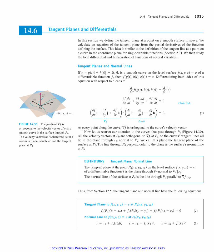
14.6 Tangent Planes and Differentials 1015
Tangent Planes and Differentials
In this section we define the tangent plane at a point on a smooth surface in space. Wecalculate an equation of the tangent plane from the partial derivatives of the functiondefining the surface. This idea is similar to the definition of the tangent line at a point ona curve in the coordinate plane for single-variable functions (Section 2.7). We then studythe total differential and linearization of functions of several variables.
Tangent Planes and Normal Lines
If is a smooth curve on the level surface of adifferentiable function ƒ, then Differentiating both sides of thisequation with respect to t leads to
(1)
At every point along the curve, is orthogonal to the curve’s velocity vector.Now let us restrict our attention to the curves that pass through (Figure 14.30).
All the velocity vectors at are orthogonal to at so the curves’ tangent lines alllie in the plane through normal to We call this plane the tangent plane of thesurface at The line through perpendicular to the plane is the surface’s normal lineat P0.
P0P0.§ƒ.P0
P0,§ƒP0
P0
§ƒ
dr>dt§ƒ
('''')''''*('''')''''*
a0ƒ0x i +
0ƒ0y j +
0ƒ0z kb # adg
dt i +
dhdt
j +
dkdt
kb = 0.
0ƒ0x
dgdt
+
0ƒ0y
dhdt
+
0ƒ0z
dkdt
= 0
ddt
ƒsgstd, hstd, kstdd =
ddt
scd
ƒsgstd, hstd, kstdd = c.ƒsx, y, zd = cr = gstdi + hstdj + kstdk
14.6
Chain Rule
∇fv2
v1P0
f (x, y, z) � c
FIGURE 14.30 The gradient isorthogonal to the velocity vector of everysmooth curve in the surface through The velocity vectors at therefore lie in acommon plane, which we call the tangentplane at P0.
P0
P0.
§ƒ
DEFINITIONS Tangent Plane, Normal Line
The tangent plane at the point on the level surface of a differentiable function ƒ is the plane through normal to
The normal line of the surface at is the line through parallel to §ƒ ƒ P0.P0P0
§ƒ ƒ P0.P0
ƒsx, y, zd = cP0sx0 , y0 , z0d
Thus, from Section 12.5, the tangent plane and normal line have the following equations:
Tangent Plane to at
(2)
Normal Line to at
(3)x = x0 + ƒxsP0dt, y = y0 + ƒysP0dt, z = z0 + ƒzsP0dt
P0sx0 , y0 , z0dƒsx, y, zd = c
ƒxsP0dsx - x0d + ƒysP0dsy - y0d + ƒzsP0dsz - z0d = 0
P0sx0 , y0, z0dƒsx, y, zd = c
4100 AWL/Thomas_ch14p965-1066 8/25/04 2:53 PM Page 1015
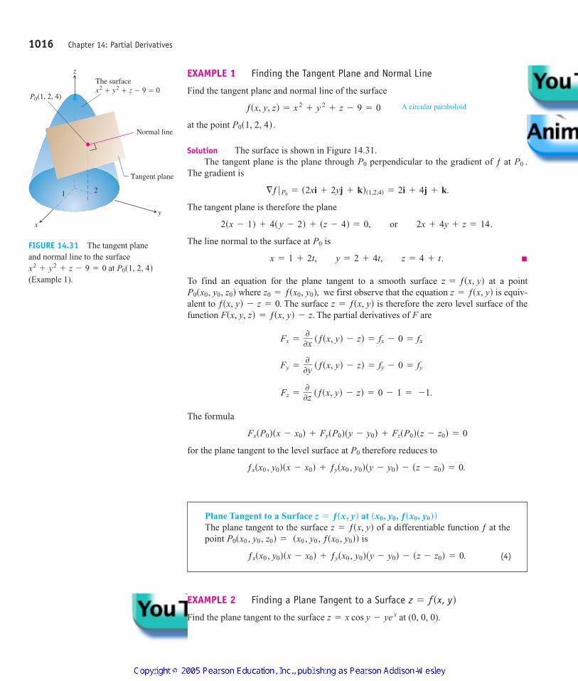
EXAMPLE 1 Finding the Tangent Plane and Normal Line
Find the tangent plane and normal line of the surface
at the point
Solution The surface is shown in Figure 14.31.The tangent plane is the plane through perpendicular to the gradient of ƒ at
The gradient is
The tangent plane is therefore the plane
The line normal to the surface at is
To find an equation for the plane tangent to a smooth surface at a pointwhere we first observe that the equation is equiv-
alent to The surface is therefore the zero level surface of thefunction The partial derivatives of F are
The formula
for the plane tangent to the level surface at therefore reduces to
ƒxsx0 , y0dsx - x0d + ƒysx0 , y0dsy - y0d - sz - z0d = 0.
P0
FxsP0dsx - x0d + FysP0dsy - y0d + FzsP0dsz - z0d = 0
Fz =
0
0z sƒsx, yd - zd = 0 - 1 = -1.
Fy =
0
0y sƒsx, yd - zd = fy - 0 = fy
Fx =
0
0x sƒsx, yd - zd = fx - 0 = fx
Fsx, y, zd = ƒsx, yd - z.z = ƒsx, ydƒsx, yd - z = 0.
z = ƒsx, ydz0 = ƒsx0, y0d,P0sx0, y0, z0dz = ƒsx, yd
x = 1 + 2t, y = 2 + 4t, z = 4 + t.
P0
2sx - 1d + 4s y - 2d + sz - 4d = 0, or 2x + 4y + z = 14.
§ƒ ƒ P0 = s2xi + 2yj + kds1,2,4d = 2i + 4j + k.
P0 .P0
P0s1, 2, 4d .
ƒsx, y, zd = x 2+ y 2
+ z - 9 = 0
1016 Chapter 14: Partial Derivatives
A circular paraboloid
z
y
x
Normal line
21
Tangent plane
The surfacex2 � y2 � z � 9 � 0
P0(1, 2, 4)
FIGURE 14.31 The tangent plane and normal line to the surface
at (Example 1).
P0s1, 2, 4dx2+ y2
+ z - 9 = 0
Plane Tangent to a Surface at The plane tangent to the surface of a differentiable function ƒ at thepoint is
(4)ƒxsx0 , y0dsx - x0d + ƒysx0 , y0dsy - y0d - sz - z0d = 0.
sx0 , y0 , ƒsx0 , y0ddP0sx0 , y0 , z0d =
z = ƒsx, ydsx0, y0, ƒsx0, y0ddz = ƒsx, yd
EXAMPLE 2 Finding a Plane Tangent to a Surface
Find the plane tangent to the surface at (0, 0, 0).z = x cos y - ye x
z = ƒsx, yd
4100 AWL/Thomas_ch14p965-1066 8/25/04 2:53 PM Page 1016
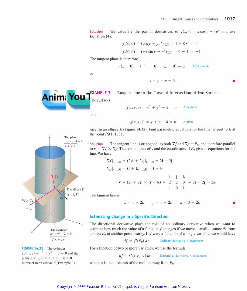
Solution We calculate the partial derivatives of and useEquation (4):
The tangent plane is therefore
or
EXAMPLE 3 Tangent Line to the Curve of Intersection of Two Surfaces
The surfaces
and
meet in an ellipse E (Figure 14.32). Find parametric equations for the line tangent to E atthe point
Solution The tangent line is orthogonal to both and at and therefore parallelto The components of v and the coordinates of give us equations for theline. We have
The tangent line is
Estimating Change in a Specific Direction
The directional derivative plays the role of an ordinary derivative when we want toestimate how much the value of a function ƒ changes if we move a small distance ds froma point to another point nearby. If ƒ were a function of a single variable, we would have
For a function of two or more variables, we use the formula
where u is the direction of the motion away from P0.
dƒ = s§ƒ ƒ P0# ud ds,
dƒ = ƒ¿sP0d ds.
P0
x = 1 + 2t, y = 1 - 2t, z = 3 - 2t.
v = s2i + 2jd * si + kd = 3 i j k
2 2 0
1 0 1
3 = 2i - 2j - 2k.
§g ƒ s1,1,3d = si + kds1,1,3d = i + k
§ƒ ƒ s1,1,3d = s2xi + 2yjds1,1,3d = 2i + 2j
P0v = §ƒ * §g.P0,§g§ƒ
P0s1, 1, 3d .
gsx, y, zd = x + z - 4 = 0
ƒsx, y, zd = x 2+ y 2
- 2 = 0
x - y - z = 0.
1 # sx - 0d - 1 # s y - 0d - sz - 0d = 0,
ƒys0, 0d = s -x sin y - e xds0,0d = 0 - 1 = -1.
ƒxs0, 0d = scos y - ye xds0,0d = 1 - 0 # 1 = 1
ƒsx, yd = x cos y - yex
14.6 Tangent Planes and Differentials 1017
Equation (4)
A cylinder
A plane
Ordinary derivative * increment
Directional derivative * increment
z
y
x
∇g
(1, 1, 3)∇f
The cylinderx2 � y2 � 2 � 0
f (x, y, z)
∇f � ∇g
The planex � z � 4 � 0
g(x, y, z)
The ellipse E
FIGURE 14.32 The cylinderand the
plane intersect in an ellipse E (Example 3).
gsx, y, zd = x + z - 4 = 0ƒsx, y, zd = x 2
+ y 2- 2 = 0
4100 AWL/Thomas_ch14p965-1066 8/25/04 2:53 PM Page 1017

EXAMPLE 4 Estimating Change in the Value of ƒ(x, y, z)
Estimate how much the value of
will change if the point P(x, y, z) moves 0.1 unit from straight toward
Solution We first find the derivative of ƒ at in the direction of the vector The direction of this vector is
The gradient of ƒ at is
Therefore,
The change dƒ in ƒ that results from moving unit away from in the directionof u is approximately
How to Linearize a Function of Two Variables
Functions of two variables can be complicated, and we sometimes need to replace themwith simpler ones that give the accuracy required for specific applications without beingso difficult to work with. We do this in a way that is similar to the way we find linearreplacements for functions of a single variable (Section 3.8).
Suppose the function we wish to replace is and that we want thereplacement to be effective near a point at which we know the values of and
and at which ƒ is differentiable. If we move from to any point (x, y) by incrementsand then the definition of differentiability from Section 14.3
gives the change
ƒsx, yd - ƒsx0, y0d = fxsx0, y0d¢x + ƒysx0, y0d¢y + P1¢x + P2¢y,
¢y = y - y0,¢x = x - x0
sx0, y0dƒy
ƒ, ƒx,sx0, y0dz = ƒsx, yd
dƒ = s§ƒ ƒ P0# udsdsd = a- 2
3bs0.1d L -0.067 unit.
P0ds = 0.1
§ƒ ƒ P0# u = si + 2kd # a2
3 i +
13
j -23
kb =23
-43
= -23
.
§ƒ ƒ s0,1,0d = ss y cos xdi + ssin x + 2zdj + 2ykdds0,1,0d = i + 2k.
P0
u =
P0 P11
ƒ P0 P11
ƒ
=
P0 P11
3=
23
i +13
j -23
k.
2i + j - 2k.P0P11
=P0
P1s2, 2, -2d.P0s0, 1, 0d
ƒsx, y, zd = y sin x + 2yz
1018 Chapter 14: Partial Derivatives
Estimating the Change in ƒ in a Direction uTo estimate the change in the value of a differentiable function ƒ when we move asmall distance ds from a point in a particular direction u, use the formula
Directional Distancederivative increment
()*('')''*
dƒ = s§ƒ ƒ P0# ud # ds
P0
4100 AWL/Thomas_ch14p965-1066 8/25/04 2:53 PM Page 1018
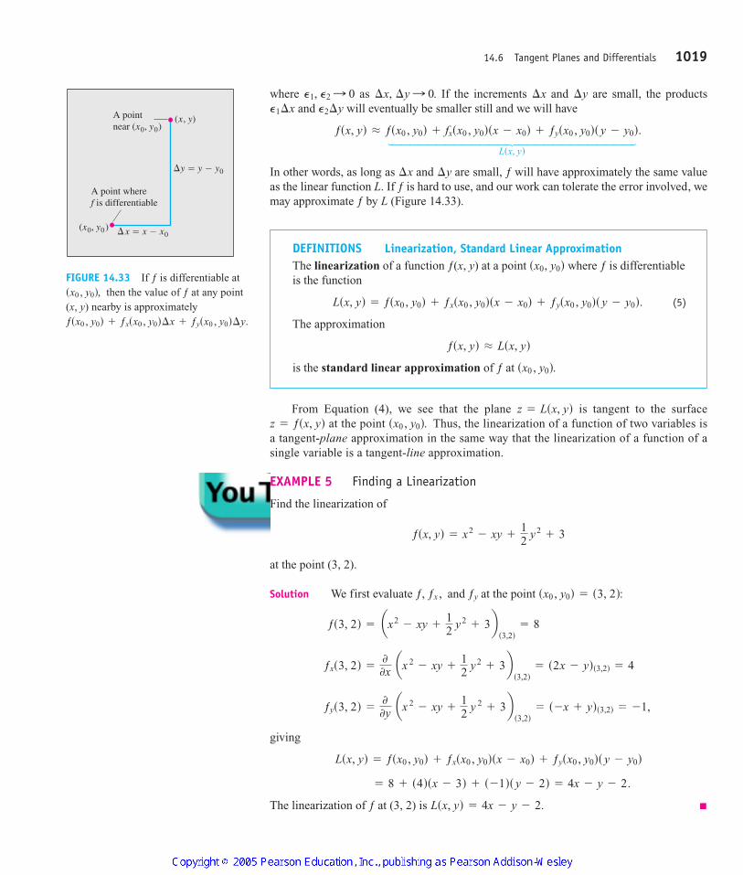
where as If the increments and are small, the productsand will eventually be smaller still and we will have
In other words, as long as and are small, ƒ will have approximately the same valueas the linear function L. If ƒ is hard to use, and our work can tolerate the error involved, wemay approximate ƒ by L (Figure 14.33).
¢y¢x
Lsx, yd(''''''''''''')'''''''''''''*
ƒsx, yd L ƒsx0 , y0d + fxsx0 , y0dsx - x0d + ƒysx0 , y0ds y - y0d.
P2¢yP1¢x¢y¢x¢x, ¢y : 0.P1, P2 : 0
14.6 Tangent Planes and Differentials 1019
A pointnear (x0, y0)
(x, y)
y � y � y0
x � x � x0(x0, y0)
A point wheref is differentiable
FIGURE 14.33 If ƒ is differentiable atthen the value of ƒ at any point
(x, y) nearby is approximatelyƒsx0 , y0d + ƒxsx0 , y0d¢x + ƒysx0 , y0d¢y.
sx0 , y0d,
DEFINITIONS Linearization, Standard Linear ApproximationThe linearization of a function ƒ(x, y) at a point where ƒ is differentiableis the function
(5)
The approximation
is the standard linear approximation of ƒ at sx0 , y0d.
ƒsx, yd L Lsx, yd
Lsx, yd = ƒsx0 , y0d + ƒxsx0 , y0dsx - x0d + ƒysx0 , y0ds y - y0d.
sx0, y0d
From Equation (4), we see that the plane is tangent to the surfaceat the point Thus, the linearization of a function of two variables is
a tangent-plane approximation in the same way that the linearization of a function of asingle variable is a tangent-line approximation.
EXAMPLE 5 Finding a Linearization
Find the linearization of
at the point (3, 2).
Solution We first evaluate and at the point
giving
The linearization of ƒ at (3, 2) is Lsx, yd = 4x - y - 2.
= 8 + s4dsx - 3d + s -1ds y - 2d = 4x - y - 2.
Lsx, yd = ƒsx0 , y0d + ƒxsx0 , y0dsx - x0d + ƒysx0 , y0ds y - y0d
ƒys3, 2d =
0
0y ax 2- xy +
12
y 2+ 3b
s3,2d= s -x + yds3,2d = -1,
ƒxs3, 2d =
0
0x ax 2- xy +
12
y2+ 3b
s3,2d= s2x - yds3,2d = 4
ƒs3, 2d = ax2- xy +
12
y2+ 3b
s3,2d= 8
sx0 , y0d = s3, 2d:ƒyƒ, ƒx ,
ƒsx, yd = x2- xy +
12
y2+ 3
sx0 , y0d.z = ƒsx, ydz = Lsx, yd
4100 AWL/Thomas_ch14p965-1066 8/25/04 2:53 PM Page 1019
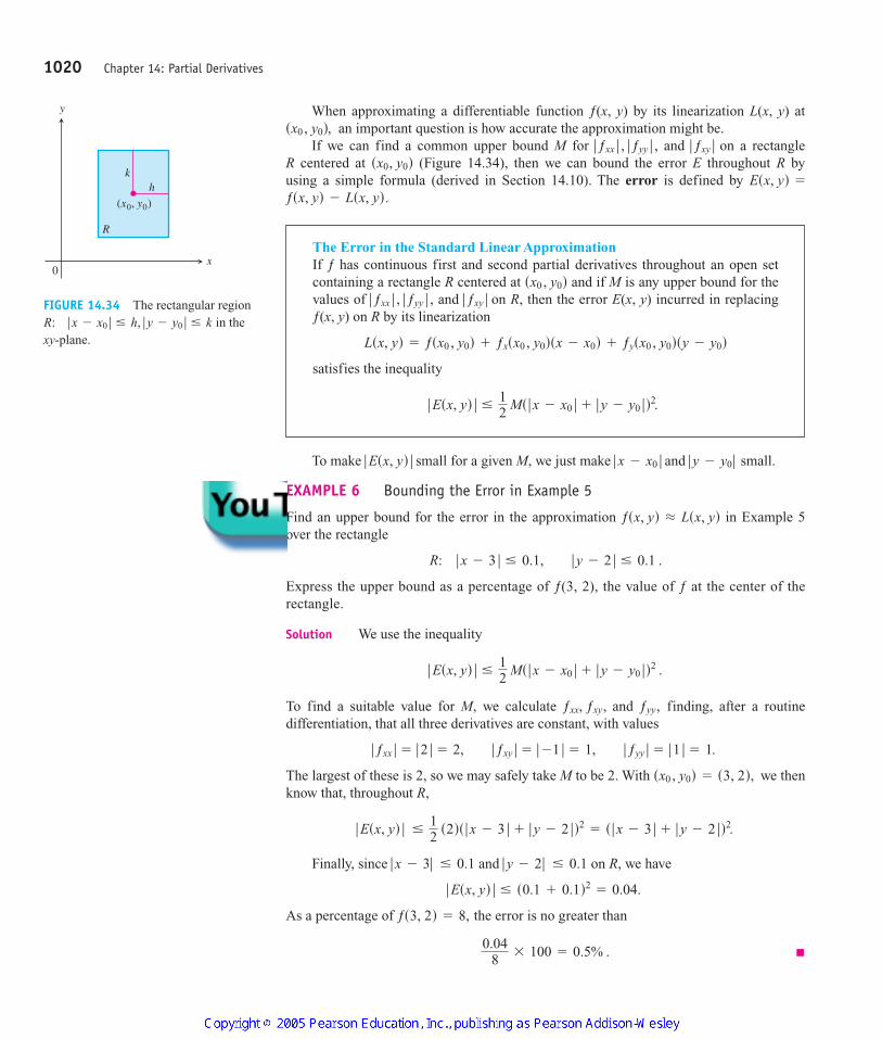
When approximating a differentiable function ƒ(x, y) by its linearization L(x, y) atan important question is how accurate the approximation might be.
If we can find a common upper bound M for and on a rectangle R centered at (Figure 14.34), then we can bound the error E throughout R by using a simple formula (derived in Section 14.10). The error is defined by ƒsx, yd - Lsx, yd.
Esx, yd =
sx0, y0dƒ ƒxy ƒƒ ƒxx ƒ , ƒ ƒyy ƒ ,
sx0 , y0d,
1020 Chapter 14: Partial Derivatives
The Error in the Standard Linear ApproximationIf ƒ has continuous first and second partial derivatives throughout an open setcontaining a rectangle R centered at and if M is any upper bound for thevalues of and on R, then the error E(x, y) incurred in replacingƒ(x, y) on R by its linearization
satisfies the inequality
ƒ Esx, yd ƒ …12
Ms ƒ x - x0 ƒ + ƒ y - y0 ƒ d2.
Lsx, yd = ƒsx0 , y0d + ƒxsx0 , y0dsx - x0d + ƒysx0 , y0dsy - y0d
ƒ ƒxy ƒƒ ƒxx ƒ , ƒ ƒyy ƒ ,sx0 , y0d
y
x0
kh
R
(x0, y0)
FIGURE 14.34 The rectangular regionin the
xy-plane.R: ƒ x - x0 ƒ … h, ƒ y - y0 ƒ … k
To make small for a given M, we just make and small.
EXAMPLE 6 Bounding the Error in Example 5
Find an upper bound for the error in the approximation in Example 5over the rectangle
Express the upper bound as a percentage of ƒ(3, 2), the value of ƒ at the center of therectangle.
Solution We use the inequality
To find a suitable value for M, we calculate and finding, after a routinedifferentiation, that all three derivatives are constant, with values
The largest of these is 2, so we may safely take M to be 2. With we thenknow that, throughout R,
Finally, since and on R, we have
As a percentage of the error is no greater than
0.048
* 100 = 0.5% .
ƒs3, 2d = 8,
ƒ Esx, yd ƒ … s0.1 + 0.1d2= 0.04.
ƒ y - 2 ƒ … 0.1ƒ x - 3 ƒ … 0.1
ƒ Esx, yd ƒ …12
s2ds ƒ x - 3 ƒ + ƒ y - 2 ƒ d2= s ƒ x - 3 ƒ + ƒ y - 2 ƒ d2.
sx0 , y0d = s3, 2d,
ƒ ƒxx ƒ = ƒ 2 ƒ = 2, ƒ ƒxy ƒ = ƒ -1 ƒ = 1, ƒ ƒyy ƒ = ƒ 1 ƒ = 1.
ƒyy,ƒxx, ƒxy,
ƒ Esx, yd ƒ …12
Ms ƒ x - x0 ƒ + ƒ y - y0 ƒ d2 .
R: ƒ x - 3 ƒ … 0.1, ƒ y - 2 ƒ … 0.1 .
ƒsx, yd L Lsx, yd
ƒ y - y0 ƒƒ x - x0 ƒƒ Esx, yd ƒ
4100 AWL/Thomas_ch14p965-1066 8/25/04 2:53 PM Page 1020
Differentials
Recall from Section 3.8 that for a function of a single variable, we defined thechange in ƒ as x changes from a to by
and the differential of ƒ as
We now consider a function of two variables.Suppose a differentiable function ƒ(x, y) and its partial derivatives exist at a point
If we move to a nearby point the change in ƒ is
A straightforward calculation from the definition of L(x, y), using the notation and shows that the corresponding change in L is
The differentials dx and dy are independent variables, so they can be assigned any values.Often we take and We then have the followingdefinition of the differential or total differential of ƒ.
dy = ¢y = y - y0 .dx = ¢x = x - x0 ,
= ƒxsx0 , y0d¢x + ƒysx0 , y0d¢y.
¢L = Lsx0 + ¢x, y0 + ¢yd - Lsx0 , y0d
y - y0 = ¢y,x - x0 = ¢x
¢ƒ = ƒsx0 + ¢x, y0 + ¢yd - ƒsx0 , y0d.
sx0 + ¢x, y0 + ¢yd,sx0 , y0d.
dƒ = ƒ¿sad¢x.
¢ƒ = ƒsa + ¢xd - ƒsad
a + ¢xy = ƒsxd,
14.6 Tangent Planes and Differentials 1021
DEFINITION Total DifferentialIf we move from to a point nearby, the resulting change
in the linearization of ƒ is called the total differential of ƒ.
dƒ = ƒxsx0 , y0d dx + ƒysx0 , y0d dy
sx0 + dx, y0 + dydsx0 , y0d
EXAMPLE 7 Estimating Change in Volume
Suppose that a cylindrical can is designed to have a radius of 1 in. and a height of 5 in., butthat the radius and height are off by the amounts and Estimatethe resulting absolute change in the volume of the can.
Solution To estimate the absolute change in we use
With and we get
= 0.3p - 0.1p = 0.2p L 0.63 in.3
dV = 2pr0h0 dr + pr02 dh = 2ps1ds5ds0.03d + ps1d2s -0.1d
Vh = pr2,Vr = 2prh
¢V L dV = Vrsr0 , h0d dr + Vhsr0 , h0d dh.
V = pr2h,
dh = -0.1.dr = +0.03
4100 AWL/Thomas_ch14p965-1066 8/25/04 2:53 PM Page 1021
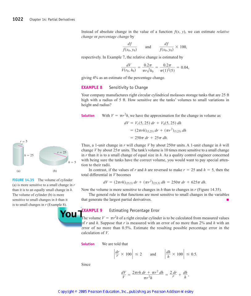
Instead of absolute change in the value of a function ƒ(x, y), we can estimate relativechange or percentage change by
respectively. In Example 7, the relative change is estimated by
giving 4% as an estimate of the percentage change.
EXAMPLE 8 Sensitivity to Change
Your company manufactures right circular cylindrical molasses storage tanks that are 25 fthigh with a radius of 5 ft. How sensitive are the tanks’ volumes to small variations inheight and radius?
Solution With we have the approximation for the change in volume as
Thus, a 1-unit change in r will change V by about A 1-unit change in h willchange V by about The tank’s volume is 10 times more sensitive to a small changein r than it is to a small change of equal size in h. As a quality control engineer concernedwith being sure the tanks have the correct volume, you would want to pay special atten-tion to their radii.
In contrast, if the values of r and h are reversed to make and then thetotal differential in V becomes
Now the volume is more sensitive to changes in h than to changes in r (Figure 14.35).The general rule is that functions are most sensitive to small changes in the variables
that generate the largest partial derivatives.
EXAMPLE 9 Estimating Percentage Error
The volume of a right circular cylinder is to be calculated from measured valuesof r and h. Suppose that r is measured with an error of no more than 2% and h with anerror of no more than 0.5%. Estimate the resulting possible percentage error in thecalculation of V.
Solution We are told that
Since
dVV
=
2prh dr + pr 2 dhpr 2h
=
2 drr +
dhh
,
` drr * 100 ` … 2 and ` dh
h* 100 ` … 0.5.
V = pr2h
dV = s2prhds25,5d dr + spr 2ds25,5d dh = 250p dr + 625p dh.
h = 5,r = 25
25p units.250p units.
= 250p dr + 25p dh.
= s2prhds5,25d dr + spr 2ds5,25d dh
dV = Vrs5, 25d dr + Vhs5, 25d dh
V = pr 2h,
dVVsr0, h0d
=
0.2ppr0
2h0=
0.2pps1d2s5d
= 0.04,
dƒ
ƒsx0, y0d and dƒ
ƒsx0, y0d* 100,
1022 Chapter 14: Partial Derivatives
(a) (b)
r � 5
r � 25h � 25
h � 5
FIGURE 14.35 The volume of cylinder(a) is more sensitive to a small change in rthan it is to an equally small change in h.The volume of cylinder (b) is moresensitive to small changes in h than it is to small changes in r (Example 8).
4100 AWL/Thomas_ch14p965-1066 8/25/04 2:53 PM Page 1022
we have
We estimate the error in the volume calculation to be at most 4.5%.
Functions of More Than Two Variables
Analogous results hold for differentiable functions of more than two variables.
1. The linearization of ƒ(x, y, z) at a point is
2. Suppose that R is a closed rectangular solid centered at and lying in an open regionon which the second partial derivatives of ƒ are continuous. Suppose also that
and are all less than or equal to M throughout R. Thenthe error in the approximation of ƒ by L isbounded throughout R by the inequality
3. If the second partial derivatives of ƒ are continuous and if x, y, and z change fromand by small amounts dx, dy, and dz, the total differential
gives a good approximation of the resulting change in ƒ.
EXAMPLE 10 Finding a Linear Approximation in 3-Space
Find the linearization L(x, y, z) of
at the point Find an upper bound for the error incurred in replac-ing ƒ by L on the rectangle
Solution A routine evaluation gives
Thus,
Since
ƒxy = -1, ƒxz = 0, ƒyz = 0,
ƒxx = 2, ƒyy = 0, ƒzz = -3 sin z,
Lsx, y, zd = 2 + 3sx - 2d + s -2ds y - 1d + 3sz - 0d = 3x - 2y + 3z - 2.
ƒs2, 1, 0d = 2, ƒxs2, 1, 0d = 3, ƒys2, 1, 0d = -2, ƒzs2, 1, 0d = 3.
R: ƒ x - 2 ƒ … 0.01, ƒ y - 1 ƒ … 0.02, ƒ z ƒ … 0.01.
sx0 , y0 , z0d = s2, 1, 0d .
ƒsx, y, zd = x2- xy + 3 sin z
dƒ = ƒxsP0d dx + ƒysP0d dy + ƒzsP0d dz
z0x0 , y0 ,
ƒ E ƒ …12
Ms ƒ x - x0 ƒ + ƒ y - y0 ƒ + ƒ z - z0 ƒ d2.
Esx, y, zd = ƒsx, y, zd - Lsx, y, zdƒ ƒyz ƒƒ ƒxx ƒ , ƒ ƒyy ƒ , ƒ ƒzz ƒ , ƒ ƒxy ƒ , ƒ ƒxz ƒ ,
P0
Lsx, y, zd = ƒsP0d + ƒxsP0dsx - x0d + ƒysP0ds y - y0d + ƒzsP0dsz - z0d.
P0sx0 , y0 , z0d
… 2s0.02d + 0.005 = 0.045.
… ` 2 drr ` + ` dh
h`
dVV` = ` 2
drr +
dhh`
14.6 Tangent Planes and Differentials 1023
4100 AWL/Thomas_ch14p965-1066 8/25/04 2:53 PM Page 1023
we may safely take M to be max Hence, the error incurred by replacing ƒby L on R satisfies
The error will be no greater than 0.0024.
ƒ E ƒ …12
s3ds0.01 + 0.02 + 0.01d2= 0.0024 .
ƒ -3 sin z ƒ = 3.
1024 Chapter 14: Partial Derivatives
4100 AWL/Thomas_ch14p965-1066 8/25/04 2:53 PM Page 1024
1024 Chapter 14: Partial Derivatives
EXERCISES 14.6
Tangent Planes and Normal Lines to SurfacesIn Exercises 1–8, find equations for the
(a) tangent plane and (b) normal line at the point on the givensurface.
1.
2.
3.
4.
5.
6.
7.
8.
In Exercises 9–12, find an equation for the plane that is tangent tothe given surface at the given point.
9. 10.
11. 12.
Tangent Lines to CurvesIn Exercises 13–18, find parametric equations for the line tangent tothe curve of intersection of the surfaces at the given point.
13. Surfaces:
Point: (1, 1, 1)
14. Surfaces:
Point: (1, 1, 1)
15. Surfaces:
Point: (1, 1, 1 2)
16. Surfaces:
Point: (1 2, 1, 1 2)
17. Surfaces:
Point: (1, 1, 3)
18. Surfaces:
Point: A22, 22, 4 Bx 2
+ y 2= 4, x 2
+ y 2- z = 0
= 11x 2
+ y 2+ z 2x 3
+ 3x 2y 2+ y 3
+ 4xy - z 2= 0,
>>x + y 2
+ z = 2, y = 1
>x 2
+ 2y + 2z = 4, y = 1
xyz = 1, x 2+ 2y 2
+ 3z 2= 6
x + y 2+ 2z = 4, x = 1
z = 4x 2+ y 2, s1, 1, 5dz = 2y - x, s1, 2, 1d
z = e-sx2+ y2d, s0, 0, 1dz = ln sx 2
+ y 2d, s1, 0, 0d
x2+ y2
- 2xy - x + 3y - z = -4, P0s2, -3, 18dx + y + z = 1, P0s0, 1, 0dx 2
- xy - y 2- z = 0, P0s1, 1, -1d
cos px - x2y + e xz+ yz = 4, P0s0, 1, 2d
x 2+ 2xy - y 2
+ z 2= 7, P0s1, -1, 3d
2z - x 2= 0, P0s2, 0, 2d
x 2+ y 2
- z 2= 18, P0s3, 5, -4d
x 2+ y 2
+ z 2= 3, P0s1, 1, 1d
P0
Estimating Change19. By about how much will
change if the point P(x, y, z) moves from a distanceof unit in the direction of
20. By about how much will
change as the point P(x, y, z) moves from the origin a distance ofunit in the direction of
21. By about how much will
change if the point P(x, y, z) moves from a distanceof unit toward the point
22. By about how much will
change if the point P(x, y, z) moves from a dis-tance of unit toward the origin?
23. Temperature change along a circle Suppose that the Celsiustemperature at the point (x, y) in the xy-plane is and that distance in the xy-plane is measured in meters. A particleis moving clockwise around the circle of radius 1 m centered atthe origin at the constant rate of 2 m sec.
a. How fast is the temperature experienced by the particlechanging in degrees Celsius per meter at the point
b. How fast is the temperature experienced by the particlechanging in degrees Celsius per second at P?
24. Changing temperature along a space curve The Celsius tem-perature in a region in space is given by A particle is moving in this region and its position at time t isgiven by where time is measured inseconds and distance in meters.
x = 2t2, y = 3t, z = - t2,
2x2- xyz.T sx, y, zd =
P A1>2, 23>2 B?
>
T sx, yd = x sin 2y
ds = 0.1P0s -1, -1, -1d
hsx, y, zd = cos spxyd + xz 2
P1s0, 1, 2)?ds = 0.2P0s2, -1, 0d
gsx, y, zd = x + x cos z - y sin z + y
2i + 2j - 2k?ds = 0.1
ƒsx, y, zd = e x cos yz
3i + 6j - 2k?ds = 0.1P0s3, 4, 12d
ƒsx, y, zd = ln2x 2+ y 2
+ z 2
4100 AWL/Thomas_ch14p965-1066 8/25/04 2:53 PM Page 1024
a. How fast is the temperature experienced by the particlechanging in degrees Celsius per meter when the particle is atthe point
b. How fast is the temperature experienced by the particlechanging in degrees Celsius per second at P?
Finding LinearizationsIn Exercises 25–30, find the linearization L(x, y) of the function ateach point.
25. at a. (0, 0), b. (1, 1)
26. at a. (0, 0), b. (1, 2)
27. at a. (0, 0), b. (1, 1)
28. at a. (1, 1), b. (0, 0)
29. at a. (0, 0), b.
30. at a. (0, 0), b. (1, 2)
Upper Bounds for Errors in Linear ApproximationsIn Exercises 31–36, find the linearization L(x, y) of the functionƒ(x, y) at Then find an upper bound for the magnitude of theerror in the approximation over the rectangle R.
31.
32.
33.
34.
35.
36.
Functions of Three VariablesFind the linearizations L(x, y, z) of the functions in Exercises 37–42at the given points.
37.
a. (1, 1, 1) b. (1, 0, 0) c. (0, 0, 0)
38.
a. (1, 1, 1) b. (0, 1, 0) c. (1, 0, 0)
39. at
a. (1, 0, 0) b. (1, 1, 0) c. (1, 2, 2)
ƒsx, y, zd = 2x 2+ y 2
+ z 2
ƒsx, y, zd = x 2+ y 2
+ z 2 at
ƒsx, y, zd = xy + yz + xz at
R: ƒ x - 1 ƒ … 0.2, ƒ y - 1 ƒ … 0.2
ƒsx, yd = ln x + ln y at P0s1, 1d,sUse ex
… 1.11 and ƒ cos y ƒ … 1 in estimating E.dR: ƒ x ƒ … 0.1, ƒ y ƒ … 0.1
ƒsx, yd = ex cos y at P0s0, 0d,R: ƒ x - 1 ƒ … 0.1, ƒ y - 2 ƒ … 0.1
ƒsx, yd = xy2+ y cos sx - 1d at P0s1, 2d,
sUse ƒ cos y ƒ … 1 and ƒ sin y ƒ … 1 in estimating E.dR: ƒ x ƒ … 0.2, ƒ y ƒ … 0.2
ƒsx, yd = 1 + y + x cos y at P0s0, 0d,R: ƒ x - 2 ƒ … 0.1, ƒ y - 2 ƒ … 0.1
ƒsx, yd = s1>2dx2+ xy + s1>4dy2
+ 3x - 3y + 4 at P0s2, 2d,R: ƒ x - 2 ƒ … 0.1, ƒ y - 1 ƒ … 0.1
ƒsx, yd = x2- 3xy + 5 at P0s2, 1d,
ƒsx, yd L Lsx, ydƒ E ƒP0.
ƒsx, yd = e 2y - x
s0, p>2dƒsx, yd = e x cos y
ƒsx, yd = x3y4
ƒsx, yd = 3x - 4y + 5
ƒsx, yd = sx + y + 2d2
ƒsx, yd = x 2+ y 2
+ 1
Ps8, 6, -4d?
40. at
a. b. (2, 0, 1)
41. at
a. (0, 0, 0) b. c.
42. at
a. (1, 0, 0) b. (1, 1, 0) c. (1, 1, 1)
In Exercises 43–46, find the linearization L(x, y, z) of the functionƒ(x, y, z) at Then find an upper bound for the magnitude of theerror E in the approximation over the region R.
43.
44.
45.
46.
Estimating Error; Sensitivity to Change47. Estimating maximum error Suppose that T is to be found
from the formula where x and y are found tobe 2 and ln 2 with maximum possible errors of and
Estimate the maximum possible error in the com-puted value of T.
48. Estimating volume of a cylinder About how accurately maybe calculated from measurements of r and h that are in
error by 1%?
49. Maximum percentage error If and to the nearest millimeter, what should we expect the maximumpercentage error in calculating to be?
50. Variation in electrical resistance The resistance R producedby wiring resistors of and ohms in parallel (see accompany-ing figure) can be calculated from the formula
a. Show that
b. You have designed a two-resistor circuit like the one shown onthe next page to have resistances of and
but there is always some variation inmanufacturing and the resistors received by your firm willprobably not have these exact values. Will the value of R be
R2 = 400 ohms,R1 = 100 ohms
dR = a RR1b2
dR1 + a RR2b2
dR2.
1R
=
1R1
+
1R2
.
R2R1
V = pr 2h
h = 12.0 cmr = 5.0 cm
V = pr 2h
0.02.ƒ dy ƒ =
ƒ dx ƒ = 0.1T = x se y
+ e-yd,
R: ƒ x ƒ … 0.01, ƒ y ƒ … 0.01, ƒ z - p>4 ƒ … 0.01
ƒsx, y, zd = 22 cos x sin s y + zd at P0s0, 0, p>4d
R: ƒ x - 1 ƒ … 0.01, ƒ y - 1 ƒ … 0.01, ƒ z ƒ … 0.01
ƒsx, y, zd = xy + 2yz - 3xz at P0s1, 1, 0dR: ƒ x - 1 ƒ … 0.01, ƒ y - 1 ƒ … 0.01, ƒ z - 2 ƒ … 0.08
ƒsx, y, zd = x 2+ xy + yz + s1>4dz2 at P0s1, 1, 2d
R: ƒ x - 1 ƒ … 0.01, ƒ y - 1 ƒ … 0.01, ƒ z - 2 ƒ … 0.02
ƒsx, y, zd = xz - 3yz + 2 at P0s1, 1, 2dƒsx, y, zd L Lsx, y, zd
P0.
ƒsx, y, zd = tan-1 sxyzd
a0, p
4, p
4ba0,
p
2, 0b
ƒsx, y, zd = e x+ cos s y + zd
sp>2, 1, 1dƒsx, y, zd = ssin xyd>z
14.6 Tangent Planes and Differentials 1025
4100 AWL/Thomas_ch14p965-1066 8/25/04 2:53 PM Page 1025
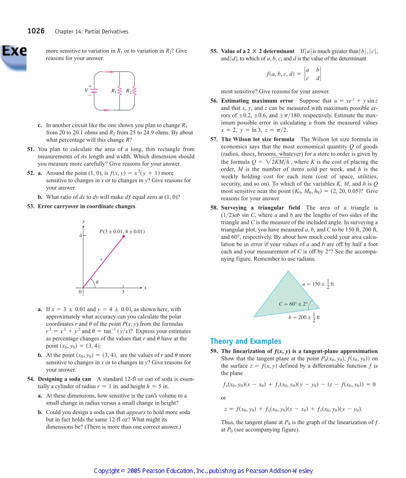
more sensitive to variation in or to variation in Givereasons for your answer.
c. In another circuit like the one shown you plan to change from 20 to 20.1 ohms and from 25 to 24.9 ohms. By aboutwhat percentage will this change R?
51. You plan to calculate the area of a long, thin rectangle frommeasurements of its length and width. Which dimension shouldyou measure more carefully? Give reasons for your answer.
52. a. Around the point (1, 0), is moresensitive to changes in x or to changes in y? Give reasons foryour answer.
b. What ratio of dx to dy will make dƒ equal zero at (1, 0)?
53. Error carryover in coordinate changes
a. If and as shown here, withapproximately what accuracy can you calculate the polarcoordinates r and of the point P(x, y) from the formulas
and Express your estimatesas percentage changes of the values that r and have at thepoint
b. At the point are the values of r and moresensitive to changes in x or to changes in y? Give reasons foryour answer.
54. Designing a soda can A standard 12-fl oz can of soda is essen-tially a cylinder of radius and height
a. At these dimensions, how sensitive is the can’s volume to asmall change in radius versus a small change in height?
b. Could you design a soda can that appears to hold more sodabut in fact holds the same 12-fl oz? What might itsdimensions be? (There is more than one correct answer.)
h = 5 in.r = 1 in.
usx0, y0d = s3, 4d,sx0, y0d = s3, 4d.
u
u = tan-1 s y>xd?r 2= x 2
+ y 2u
y = 4 ; 0.01,x = 3 ; 0.01
y
x0
4
3
r
�
P(3 ; 0.01, 4 ; 0.01)
ƒsx, yd = x 2s y + 1d
R2
R1
�
�V R1 R2
R2?R1 55. Value of a determinant If is much greater than and to which of a, b, c, and d is the value of the determinant
most sensitive? Give reasons for your answer.
56. Estimating maximum error Suppose that and that x, y, and z can be measured with maximum possible er-rors of and respectively. Estimate the max-imum possible error in calculating u from the measured values
57. The Wilson lot size formula The Wilson lot size formula ineconomics says that the most economical quantity Q of goods(radios, shoes, brooms, whatever) for a store to order is given bythe formula where K is the cost of placing theorder, M is the number of items sold per week, and h is theweekly holding cost for each item (cost of space, utilities,security, and so on). To which of the variables K, M, and h is Qmost sensitive near the point Givereasons for your answer.
58. Surveying a triangular field The area of a triangle is (1 2)ab sin C, where a and b are the lengths of two sides of thetriangle and C is the measure of the included angle. In surveying atriangular plot, you have measured a, b, and C to be 150 ft, 200 ft,and 60°, respectively. By about how much could your area calcu-lation be in error if your values of a and b are off by half a footeach and your measurement of C is off by 2°? See the accompa-nying figure. Remember to use radians.
Theory and Examples59. The linearization of ƒ(x, y) is a tangent-plane approximation
Show that the tangent plane at the point onthe surface defined by a differentiable function ƒ isthe plane
or
Thus, the tangent plane at is the graph of the linearization of ƒat (see accompanying figure).P0
P0
z = ƒsx0, y0d + ƒxsx0, y0dsx - x0d + ƒysx0, y0ds y - y0d.
ƒxsx0, y0dsx - x0d + ƒysx0, y0ds y - y0d - sz - ƒsx0, y0dd = 0
z = ƒsx, ydP0sx0, y0d, ƒsx0, y0dd
a � 150 ; ft12
b � 200 ; ft12
C � 60° ; 2°
>
sK0, M0, h0d = s2, 20, 0.05d?
Q = 22KM>h ,
x = 2, y = ln 3, z = p>2.
;p>180,;0.2, ;0.6,
u = xe y+ y sin z
ƒsa, b, c, dd = ` a b
c d`
ƒ d ƒ ,ƒ b ƒ , ƒ c ƒ ,ƒ a ƒ2 : 2
1026 Chapter 14: Partial Derivatives
4100 AWL/Thomas_ch14p965-1066 8/25/04 2:53 PM Page 1026
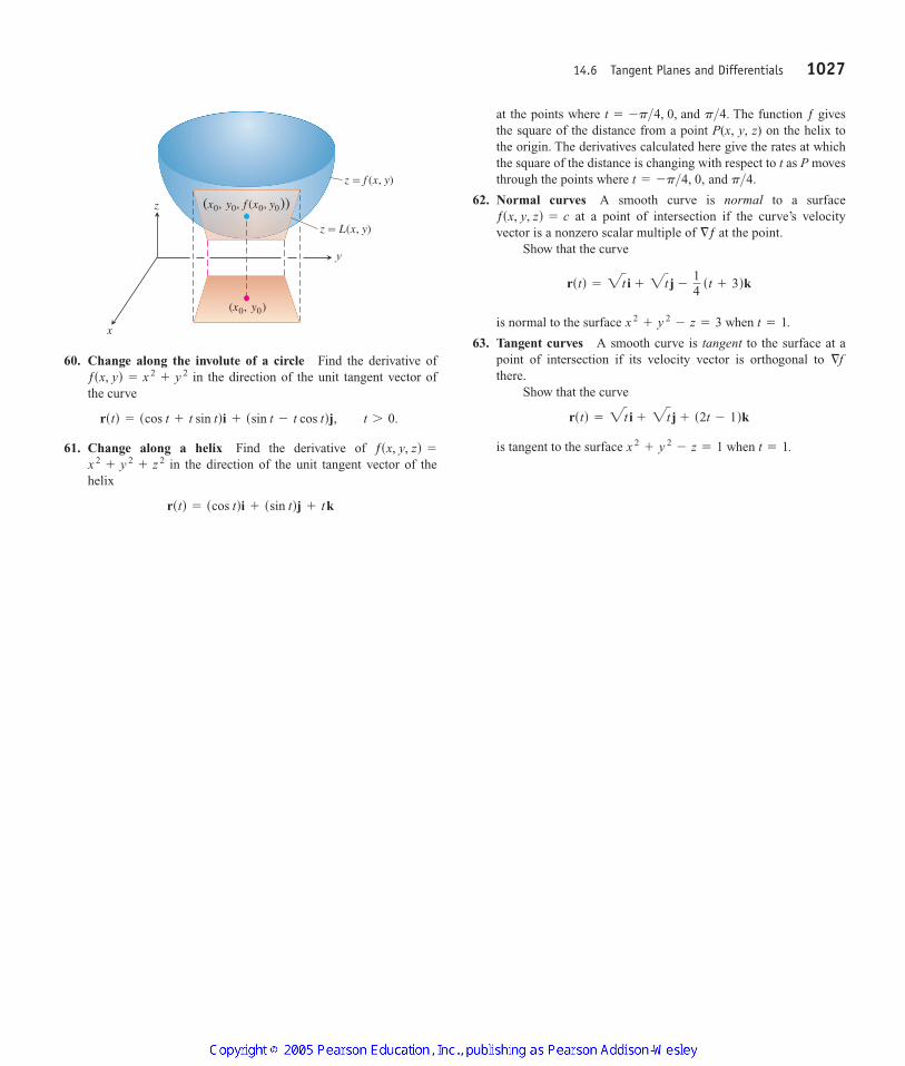
at the points where and The function ƒ givesthe square of the distance from a point P(x, y, z) on the helix tothe origin. The derivatives calculated here give the rates at whichthe square of the distance is changing with respect to t as P movesthrough the points where and
62. Normal curves A smooth curve is normal to a surfaceat a point of intersection if the curve’s velocity
vector is a nonzero scalar multiple of at the point.Show that the curve
is normal to the surface when
63. Tangent curves A smooth curve is tangent to the surface at apoint of intersection if its velocity vector is orthogonal to there.
Show that the curve
is tangent to the surface when t = 1.x 2+ y 2
- z = 1
rstd = 2t i + 2t j + s2t - 1dk
§f
t = 1.x 2+ y 2
- z = 3
rstd = 2t i + 2t j -
14
st + 3dk
§ƒƒsx, y, zd = c
p>4.t = -p>4, 0,
p>4.t = -p>4, 0,
1027
60. Change along the involute of a circle Find the derivative ofin the direction of the unit tangent vector of
the curve
61. Change along a helix Find the derivative of in the direction of the unit tangent vector of the
helix
rstd = scos tdi + ssin tdj + tk
x 2+ y 2
+ z 2ƒsx, y, zd =
rstd = scos t + t sin tdi + ssin t - t cos tdj, t 7 0.
ƒsx, yd = x 2+ y 2
z
x
y
(x0, y0)
z � L(x, y)
z � f (x, y)
(x0, y0, f (x0, y0))
4100 AWL/Thomas_ch14p965-1066 9/2/04 11:09 AM Page 1027
14.6 Tangent Planes and Differentials
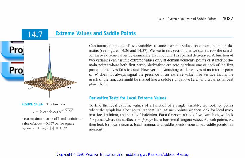
14.7 Extreme Values and Saddle Points 1027
Extreme Values and Saddle Points
Continuous functions of two variables assume extreme values on closed, bounded do-mains (see Figures 14.36 and 14.37). We see in this section that we can narrow the searchfor these extreme values by examining the functions’ first partial derivatives. A function oftwo variables can assume extreme values only at domain boundary points or at interior do-main points where both first partial derivatives are zero or where one or both of the firstpartial derivatives fails to exist. However, the vanishing of derivatives at an interior point(a, b) does not always signal the presence of an extreme value. The surface that is thegraph of the function might be shaped like a saddle right above (a, b) and cross its tangentplane there.
Derivative Tests for Local Extreme Values
To find the local extreme values of a function of a single variable, we look for pointswhere the graph has a horizontal tangent line. At such points, we then look for local max-ima, local minima, and points of inflection. For a function ƒ(x, y) of two variables, we lookfor points where the surface has a horizontal tangent plane. At such points, wethen look for local maxima, local minima, and saddle points (more about saddle points in amoment).
z = ƒsx, yd
14.7z
yx
FIGURE 14.36 The function
has a maximum value of 1 and a minimumvalue of about on the squareregion ƒ x ƒ … 3p>2, ƒ y ƒ … 3p>2.
-0.067
z = scos xdscos yde-2x 2+ y2
4100 AWL/Thomas_ch14p965-1066 9/2/04 11:09 AM Page 1027

Local maxima correspond to mountain peaks on the surface and local minimacorrespond to valley bottoms (Figure 14.38). At such points the tangent planes, when theyexist, are horizontal. Local extrema are also called relative extrema.
As with functions of a single variable, the key to identifying the local extrema is afirst derivative test.
z = ƒsx, yd
1028 Chapter 14: Partial Derivatives
z
yx
FIGURE 14.37 The “roof surface”
viewed from the point (10, 15, 20). Thedefining function has a maximum value of0 and a minimum value of on thesquare region ƒ x ƒ … a, ƒ y ƒ … a .
-a
z =
12
A ƒ ƒ x ƒ - ƒ y ƒ ƒ - ƒ x ƒ - ƒ y ƒ B
DEFINITIONS Local Maximum, Local MinimumLet ƒ(x, y) be defined on a region R containing the point (a, b). Then
1. ƒ(a, b) is a local maximum value of ƒ if for all domainpoints (x, y) in an open disk centered at (a, b).
2. ƒ(a, b) is a local minimum value of ƒ if for all domainpoints (x, y) in an open disk centered at (a, b).
ƒsa, bd … ƒsx, yd
ƒsa, bd Ú ƒsx, yd
y
x
0
z
ab
(a, b, 0)
h(y) � f (a, y)
z � f (x, y)
� 00 f0y
� 00f0x
g(x) � f (x, b)
FIGURE 14.39 If a local maximum of ƒoccurs at then the firstpartial derivatives and areboth zero.
ƒysa, bdƒxsa, bdx = a, y = b ,
Local maxima(no greater value of f nearby)
Local minimum(no smaller valueof f nearby)
FIGURE 14.38 A local maximum is a mountain peak and a localminimum is a valley low.
THEOREM 10 First Derivative Test for Local Extreme ValuesIf ƒ(x, y) has a local maximum or minimum value at an interior point (a, b) of itsdomain and if the first partial derivatives exist there, then andƒysa, bd = 0.
ƒxsa, bd = 0
HISTORICAL BIOGRAPHY
Siméon-Denis Poisson(1781–1840)
Proof If ƒ has a local extremum at (a, b), then the function has a local ex-tremum at (Figure 14.39). Therefore, (Chapter 4, Theorem 2). Now
so A similar argument with the function shows that
If we substitute the values and into the equation
for the tangent plane to the surface at (a, b), the equation reduces to
or
z = ƒsa, bd.
0 # sx - ad + 0 # s y - bd - z + ƒsa, bd = 0
z = ƒsx, yd
ƒxsa, bdsx - ad + ƒysa, bds y - bd - sz - ƒsa, bdd = 0
ƒysa, bd = 0ƒxsa, bd = 0
ƒysa, bd = 0.hsyd = ƒsa, ydƒxsa, bd = 0.g¿sad = ƒxsa, bd,
g¿sad = 0x = agsxd = ƒsx, bd
4100 AWL/Thomas_ch14p965-1066 8/25/04 2:53 PM Page 1028
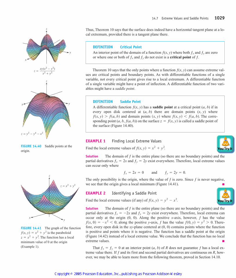
EXAMPLE 1 Finding Local Extreme Values
Find the local extreme values of
Solution The domain of ƒ is the entire plane (so there are no boundary points) and thepartial derivatives and exist everywhere. Therefore, local extreme valuescan occur only where
The only possibility is the origin, where the value of ƒ is zero. Since ƒ is never negative,we see that the origin gives a local minimum (Figure 14.41).
EXAMPLE 2 Identifying a Saddle Point
Find the local extreme values (if any) of
Solution The domain of ƒ is the entire plane (so there are no boundary points) and thepartial derivatives and exist everywhere. Therefore, local extrema canoccur only at the origin (0, 0). Along the positive x-axis, however, ƒ has the value
along the positive y-axis, ƒ has the value There-fore, every open disk in the xy-plane centered at (0, 0) contains points where the functionis positive and points where it is negative. The function has a saddle point at the origin(Figure 14.42) instead of a local extreme value. We conclude that the function has no localextreme values.
That at an interior point (a, b) of R does not guarantee ƒ has a local ex-treme value there. If ƒ and its first and second partial derivatives are continuous on R, how-ever, we may be able to learn more from the following theorem, proved in Section 14.10.
ƒx = ƒy = 0
ƒs0, yd = y27 0.ƒsx, 0d = -x2
6 0;
ƒy = 2yƒx = -2x
ƒsx, yd = y2- x2.
ƒx = 2x = 0 and ƒy = 2y = 0.
ƒy = 2yƒx = 2x
ƒsx, yd = x2+ y2.
Thus, Theorem 10 says that the surface does indeed have a horizontal tangent plane at a lo-cal extremum, provided there is a tangent plane there.
14.7 Extreme Values and Saddle Points 1029
DEFINITION Critical PointAn interior point of the domain of a function ƒ(x, y) where both and are zeroor where one or both of and do not exist is a critical point of ƒ.ƒyƒx
ƒyƒx
DEFINITION Saddle PointA differentiable function ƒ(x, y) has a saddle point at a critical point (a, b) if inevery open disk centered at (a, b) there are domain points (x, y) where
and domain points where The corre-sponding point (a, b, ƒ(a, b)) on the surface is called a saddle point ofthe surface (Figure 14.40).
z = ƒsx, ydƒsx, yd 6 ƒsa, bd.sx, ydƒsx, yd 7 ƒsa, bd
x
z
y
x
z
y
z �xy (x2 � y2)
x2 � y2
z � y2 � y4 � x2
FIGURE 14.40 Saddle points at theorigin.
z
yx
z � x2 � y2
FIGURE 14.41 The graph of the functionis the paraboloid
The function has a localminimum value of 0 at the origin(Example 1).
z = x2+ y2.
ƒsx, yd = x2+ y2
Theorem 10 says that the only points where a function ƒ(x, y) can assume extreme val-ues are critical points and boundary points. As with differentiable functions of a singlevariable, not every critical point gives rise to a local extremum. A differentiable functionof a single variable might have a point of inflection. A differentiable function of two vari-ables might have a saddle point.
4100 AWL/Thomas_ch14p965-1066 8/25/04 2:53 PM Page 1029
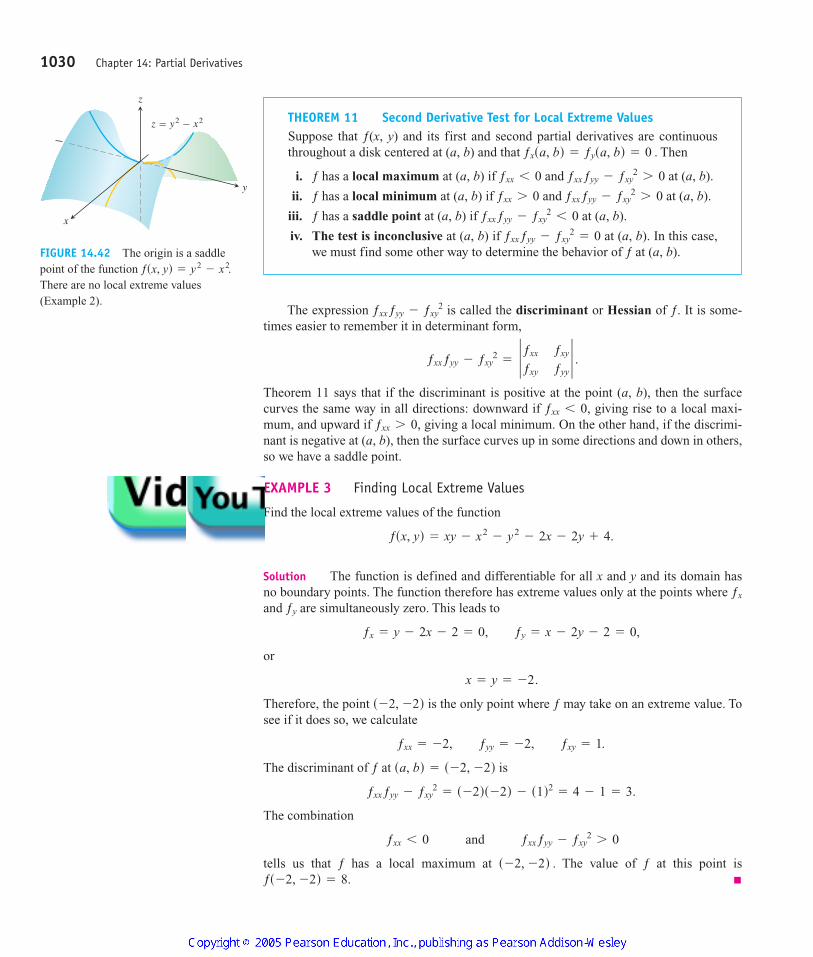
1030 Chapter 14: Partial Derivatives
y
z
x
z � y2 � x2
FIGURE 14.42 The origin is a saddlepoint of the function There are no local extreme values(Example 2).
ƒsx, yd = y2- x2.
THEOREM 11 Second Derivative Test for Local Extreme ValuesSuppose that ƒ(x, y) and its first and second partial derivatives are continuousthroughout a disk centered at (a, b) and that Then
i. ƒ has a local maximum at (a, b) if and at (a, b).
ii. ƒ has a local minimum at (a, b) if and at (a, b).
iii. ƒ has a saddle point at (a, b) if at (a, b).
iv. The test is inconclusive at (a, b) if at (a, b). In this case,we must find some other way to determine the behavior of ƒ at (a, b).
ƒxx ƒyy - ƒxy2
= 0
ƒxx ƒyy - ƒxy2
6 0
ƒxx ƒyy - ƒxy2
7 0ƒxx 7 0
ƒxx ƒyy - ƒxy2
7 0ƒxx 6 0
ƒxsa, bd = ƒysa, bd = 0 .
The expression is called the discriminant or Hessian of ƒ. It is some-times easier to remember it in determinant form,
Theorem 11 says that if the discriminant is positive at the point (a, b), then the surfacecurves the same way in all directions: downward if giving rise to a local maxi-mum, and upward if giving a local minimum. On the other hand, if the discrimi-nant is negative at (a, b), then the surface curves up in some directions and down in others,so we have a saddle point.
EXAMPLE 3 Finding Local Extreme Values
Find the local extreme values of the function
Solution The function is defined and differentiable for all x and y and its domain hasno boundary points. The function therefore has extreme values only at the points where and are simultaneously zero. This leads to
or
Therefore, the point is the only point where ƒ may take on an extreme value. Tosee if it does so, we calculate
The discriminant of ƒ at is
The combination
tells us that ƒ has a local maximum at The value of ƒ at this point isƒs -2, -2d = 8.
s -2, -2d .
ƒxx 6 0 and ƒxx ƒyy - ƒxy2
7 0
ƒxx ƒyy - ƒxy2
= s -2ds -2d - s1d2= 4 - 1 = 3.
sa, bd = s -2, -2d
ƒxx = -2, ƒyy = -2, ƒxy = 1.
s -2, -2d
x = y = -2.
ƒx = y - 2x - 2 = 0, ƒy = x - 2y - 2 = 0,
ƒy
ƒx
ƒsx, yd = xy - x2- y2
- 2x - 2y + 4.
ƒxx 7 0,ƒxx 6 0,
ƒxx ƒyy - ƒxy2
= p ƒxx ƒxy
ƒxy ƒyyp .
ƒxx ƒyy - ƒxy2
4100 AWL/Thomas_ch14p965-1066 9/2/04 11:09 AM Page 1030

EXAMPLE 4 Searching for Local Extreme Values
Find the local extreme values of
Solution Since ƒ is differentiable everywhere (Figure 14.43), it can assume extremevalues only where
Thus, the origin is the only point where ƒ might have an extreme value. To see what hap-pens there, we calculate
The discriminant,
is negative. Therefore, the function has a saddle point at (0, 0). We conclude thathas no local extreme values.
Absolute Maxima and Minima on Closed Bounded Regions
We organize the search for the absolute extrema of a continuous function ƒ(x, y) on aclosed and bounded region R into three steps.
1. List the interior points of R where ƒ may have local maxima and minima and evaluateƒ at these points. These are the critical points of ƒ.
2. List the boundary points of R where ƒ has local maxima and minima and evaluate ƒ atthese points. We show how to do this shortly.
3. Look through the lists for the maximum and minimum values of ƒ. These will be theabsolute maximum and minimum values of ƒ on R. Since absolute maxima and min-ima are also local maxima and minima, the absolute maximum and minimum valuesof ƒ appear somewhere in the lists made in Steps 1 and 2.
EXAMPLE 5 Finding Absolute Extrema
Find the absolute maximum and minimum values of
on the triangular region in the first quadrant bounded by the lines
Solution Since ƒ is differentiable, the only places where ƒ can assume these values arepoints inside the triangle (Figure 14.44) where and points on the boundary.
(a) Interior points. For these we have
yielding the single point The value of ƒ there is
ƒs1, 1d = 4.
sx, yd = s1, 1d.
fx = 2 - 2x = 0, fy = 2 - 2y = 0,
ƒx = ƒy = 0
y = 9 - x .x = 0, y = 0,
ƒsx, yd = 2 + 2x + 2y - x2- y2
ƒsx, yd = xy
ƒxx ƒyy - ƒxy2
= -1,
ƒxx = 0, ƒyy = 0, ƒxy = 1.
ƒx = y = 0 and ƒy = x = 0.
ƒsx, yd = xy.
14.7 Extreme Values and Saddle Points 1031
z y
x
z � xy
FIGURE 14.43 The surface has asaddle point at the origin (Example 4).
z = xy
y
xO
(1, 1)
x � 0
B(0, 9)
y � 9 � x
A(9, 0)y � 0
92
92
,
FIGURE 14.44 This triangular region isthe domain of the function in Example 5.
4100 AWL/Thomas_ch14p965-1066 8/25/04 2:53 PM Page 1031
(b) Boundary points. We take the triangle one side at a time:
(i) On the segment OA, The function
may now be regarded as a function of x defined on the closed interval Itsextreme values (we know from Chapter 4) may occur at the endpoints
and at the interior points where The only interior point whereis where
(ii) On the segment OB, and
We know from the symmetry of ƒ in x and y and from the analysis we just carried outthat the candidates on this segment are
(iii) We have already accounted for the values of ƒ at the endpoints of AB, so we need onlylook at the interior points of AB. With we have
Setting gives
At this value of x,
Summary We list all the candidates: The maximum is 4, which ƒassumes at (1, 1). The minimum is which ƒ assumes at (0, 9) and (9, 0).
Solving extreme value problems with algebraic constraints on the variables usually re-quires the method of Lagrange multipliers in the next section. But sometimes we can solvesuch problems directly, as in the next example.
EXAMPLE 6 Solving a Volume Problem with a Constraint
A delivery company accepts only rectangular boxes the sum of whose length and girth(perimeter of a cross-section) does not exceed 108 in. Find the dimensions of an accept-able box of largest volume.
Solution Let x, y, and z represent the length, width, and height of the rectangular box,respectively. Then the girth is We want to maximize the volume of theV = xyz2y + 2z.
-61,4, 2, -61, 3, -s41>2d.
y = 9 -
92
=
92 and ƒsx, yd = ƒ a9
2,
92b = -
412
.
x =
184
=
92
.
ƒ¿sx, 9 - xd = 18 - 4x = 0
ƒsx, yd = 2 + 2x + 2s9 - xd - x2- s9 - xd2
= -61 + 18x - 2x2.
y = 9 - x,
ƒs0, 0d = 2, ƒs0, 9d = -61, ƒs0, 1d = 3.
ƒsx, yd = ƒs0, yd = 2 + 2y - y2.
x = 0
ƒsx, 0d = ƒs1, 0d = 3.
x = 1,ƒ¿sx, 0d = 0ƒ¿sx, 0d = 2 - 2x = 0.
x = 9 where ƒs9, 0d = 2 + 18 - 81 = -61
x = 0 where ƒs0, 0d = 2
0 … x … 9.
ƒsx, yd = ƒsx, 0d = 2 + 2x - x2
y = 0.
1032 Chapter 14: Partial Derivatives
4100 AWL/Thomas_ch14p965-1066 8/25/04 2:53 PM Page 1032
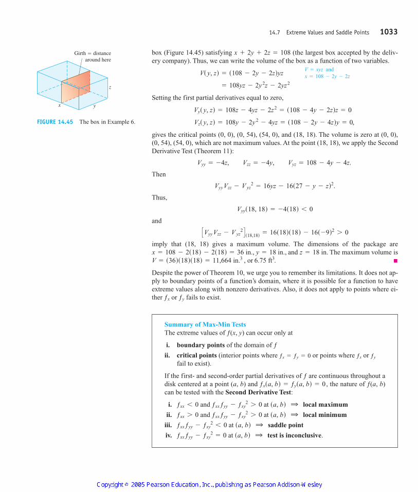
box (Figure 14.45) satisfying (the largest box accepted by the deliv-ery company). Thus, we can write the volume of the box as a function of two variables.
Setting the first partial derivatives equal to zero,
gives the critical points (0, 0), (0, 54), (54, 0), and (18, 18). The volume is zero at (0, 0),(0, 54), (54, 0), which are not maximum values. At the point (18, 18), we apply the SecondDerivative Test (Theorem 11):
Then
Thus,
and
imply that (18, 18) gives a maximum volume. The dimensions of the package areand The maximum volume is
or
Despite the power of Theorem 10, we urge you to remember its limitations. It does not ap-ply to boundary points of a function’s domain, where it is possible for a function to haveextreme values along with nonzero derivatives. Also, it does not apply to points where ei-ther or fails to exist.ƒyƒx
6.75 ft3.V = s36ds18ds18d = 11,664 in.3 ,z = 18 in.x = 108 - 2s18d - 2s18d = 36 in., y = 18 in.,
CVyy Vzz - V yz2 D s18,18d = 16s18ds18d - 16s -9d2
7 0
Vyys18, 18d = -4s18d 6 0
Vyy Vzz - V yz2
= 16yz - 16s27 - y - zd2.
Vyy = -4z, Vzz = -4y, Vyz = 108 - 4y - 4z.
Vzs y, zd = 108y - 2y2- 4yz = s108 - 2y - 4zdy = 0,
Vys y, zd = 108z - 4yz - 2z2= s108 - 4y - 2zdz = 0
= 108yz - 2y2z - 2yz2
Vs y, zd = s108 - 2y - 2zdyz
x + 2y + 2z = 108
14.7 Extreme Values and Saddle Points 1033
x y
z
Girth � distancearound here
FIGURE 14.45 The box in Example 6.
andx = 108 - 2y - 2zV = xyz
Summary of Max-Min TestsThe extreme values of ƒ(x, y) can occur only at
i. boundary points of the domain of ƒ
ii. critical points (interior points where or points where or fail to exist).
If the first- and second-order partial derivatives of ƒ are continuous throughout adisk centered at a point (a, b) and the nature of ƒ(a, b)can be tested with the Second Derivative Test:
i. and at
ii. and at
iii. at
iv. at sa, bd Q test is inconclusive.ƒxx ƒyy - ƒxy2
= 0
sa, bd Q saddle pointƒxx ƒyy - ƒxy2
6 0
sa, bd Q local minimumƒxx ƒyy - ƒxy2
7 0ƒxx 7 0
sa, bd Q local maximumƒxx ƒyy - ƒxy2
7 0ƒxx 6 0
ƒxsa, bd = ƒysa, bd = 0,
ƒyƒxƒx = ƒy = 0
4100 AWL/Thomas_ch14p965-1066 8/25/04 2:53 PM Page 1033
1034 Chapter 14: Partial Derivatives
EXERCISES 14.7
Finding Local ExtremaFind all the local maxima, local minima, and saddle points of thefunctions in Exercises 1–30.
1.
2.
3.
4.
5.
6.
7.
8.
9.
10.
11.
12.
13.
14.
15.
16.
17.
18.
19.
20.
21.
22.
23.
24.
25.
26.
27. 28.
29. 30.
Finding Absolute ExtremaIn Exercises 31–38, find the absolute maxima and minima of the func-tions on the given domains.
31. on the closed triangularplate bounded by the lines in the firstquadrant
32. on the closed triangular plate in thefirst quadrant bounded by the lines x = 0, y = 4, y = xDsx, yd = x2
- xy + y2+ 1
x = 0, y = 2, y = 2xƒsx, yd = 2x2
- 4x + y2- 4y + 1
ƒsx, yd = e2x cos yƒsx, yd = y sin x
ƒsx, yd =
1x + xy +
1yƒsx, yd =
1x2
+ y2- 1
ƒsx, yd = x4+ y4
+ 4xy
ƒsx, yd = 4xy - x4- y4
ƒsx, yd = 2x3+ 2y3
- 9x2+ 3y2
- 12y
ƒsx, yd = x3+ y3
+ 3x2- 3y2
- 8
ƒsx, yd = 8x3+ y3
+ 6xy
ƒsx, yd = 9x3+ y3>3 - 4xy
ƒsx, yd = 3y2- 2y3
- 3x2+ 6xy
ƒsx, yd = 6x2- 2x3
+ 3y2+ 6xy
ƒsx, yd = x3+ 3xy + y3
ƒsx, yd = x3- y3
- 2xy + 6
ƒsx, yd = 3 + 2x + 2y - 2x2- 2xy - y2
ƒsx, yd = x2+ 2xy
ƒsx, yd = x2- 2xy + 2y2
- 2x + 2y + 1
ƒsx, yd = x2- y2
- 2x + 4y + 6
ƒsx, yd = 4x2- 6xy + 5y2
- 20x + 26y
ƒsx, yd = 2x2+ 3xy + 4y2
- 5x + 2y
ƒsx, yd = 3x2+ 6xy + 7y2
- 2x + 4y
ƒsx, yd = x2- 4xy + y2
+ 6y + 2
ƒsx, yd = 2xy - x2- 2y2
+ 3x + 4
ƒsx, yd = 5xy - 7x2+ 3x - 6y + 2
ƒsx, yd = y2+ xy - 2x - 2y + 2
ƒsx, yd = x2+ xy + 3x + 2y + 5
ƒsx, yd = 2xy - 5x2- 2y2
+ 4x - 4
ƒsx, yd = 2xy - 5x2- 2y2
+ 4x + 4y - 4
ƒsx, yd = x2+ 3xy + 3y2
- 6x + 3y - 6
ƒsx, yd = x2+ xy + y2
+ 3x - 3y + 4
33. on the closed triangular plate bounded by thelines in the first quadrant
34. on the rectangular plate
35. on the rectangular plate
36. on the rectangular plate
37. on the rectangular plate (see accompanying figure).
38. on the triangular plate bounded bythe lines in the first quadrant
39. Find two numbers a and b with such that
has its largest value.
40. Find two numbers a and b with such that
has its largest value.
41. Temperatures The flat circular plate in Figure 14.46 has theshape of the region The plate, including theboundary where is heated so that the temperatureat the point (x, y) is
Find the temperatures at the hottest and coldest points on theplate.
Tsx, yd = x2+ 2y2
- x.
x2+ y2
= 1 ,x2
+ y2… 1.
Lb
as24 - 2x - x2d1>3 dx
a … b
Lb
as6 - x - x2d dx
a … b
x = 0, y = 0, x + y = 1ƒsx, yd = 4x - 8xy + 2y + 1
z
yx
z � (4x � x2) cos y
-p>4 … y … p>4 1 … x … 3, ƒsx, yd = s4x - x2d cos y
1, 0 … y … 10 … x …
ƒsx, yd = 48xy - 32x3- 24y2
0 … x … 5, -3 … y … 0Tsx, yd = x2
+ xy + y2- 6x + 2
0 … x … 5, -3 … y … 3Tsx, yd = x2
+ xy + y2- 6x
x = 0, y = 0, y + 2x = 2ƒsx, yd = x2
+ y2
4100 AWL/Thomas_ch14p965-1066 8/25/04 2:53 PM Page 1034
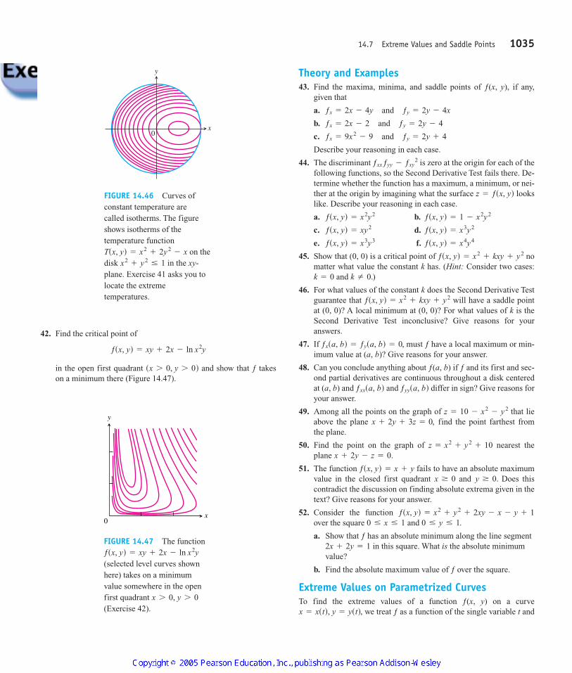
42. Find the critical point of
in the open first quadrant and show that ƒ takeson a minimum there (Figure 14.47).
sx 7 0, y 7 0d
ƒsx, yd = xy + 2x - ln x2y
Theory and Examples43. Find the maxima, minima, and saddle points of ƒ(x, y), if any,
given that
a.
b.
c.
Describe your reasoning in each case.
44. The discriminant is zero at the origin for each of thefollowing functions, so the Second Derivative Test fails there. De-termine whether the function has a maximum, a minimum, or nei-ther at the origin by imagining what the surface lookslike. Describe your reasoning in each case.
a. b.
c. d.
e. f.
45. Show that (0, 0) is a critical point of nomatter what value the constant k has. (Hint: Consider two cases:
and )
46. For what values of the constant k does the Second Derivative Testguarantee that will have a saddle pointat (0, 0)? A local minimum at (0, 0)? For what values of k is theSecond Derivative Test inconclusive? Give reasons for youranswers.
47. If must ƒ have a local maximum or min-imum value at (a, b)? Give reasons for your answer.
48. Can you conclude anything about ƒ(a, b) if ƒ and its first and sec-ond partial derivatives are continuous throughout a disk centeredat (a, b) and and differ in sign? Give reasons foryour answer.
49. Among all the points on the graph of that lieabove the plane find the point farthest fromthe plane.
50. Find the point on the graph of nearest theplane
51. The function fails to have an absolute maximumvalue in the closed first quadrant and Does thiscontradict the discussion on finding absolute extrema given in thetext? Give reasons for your answer.
52. Consider the function over the square and
a. Show that ƒ has an absolute minimum along the line segmentin this square. What is the absolute minimum
value?
b. Find the absolute maximum value of ƒ over the square.
Extreme Values on Parametrized CurvesTo find the extreme values of a function ƒ(x, y) on a curve
we treat ƒ as a function of the single variable t andx = xstd, y = ystd,
2x + 2y = 1
0 … y … 1.0 … x … 1ƒsx, yd = x2
+ y2+ 2xy - x - y + 1
y Ú 0.x Ú 0ƒsx, yd = x + y
x + 2y - z = 0.z = x2
+ y2+ 10
x + 2y + 3z = 0,z = 10 - x2
- y2
ƒyysa, bdƒxxsa, bd
ƒxsa, bd = ƒysa, bd = 0,
ƒsx, yd = x2+ kxy + y2
k Z 0.k = 0
ƒsx, yd = x2+ kxy + y2
ƒsx, yd = x4y4ƒsx, yd = x3y3
ƒsx, yd = x3y2ƒsx, yd = xy2
ƒsx, yd = 1 - x2y2ƒsx, yd = x2y2
z = ƒsx, yd
ƒxx ƒyy - ƒxy2
ƒx = 9x2- 9 and ƒy = 2y + 4
ƒx = 2x - 2 and ƒy = 2y - 4
ƒx = 2x - 4y and ƒy = 2y - 4x
14.7 Extreme Values and Saddle Points 1035
y
x0
FIGURE 14.46 Curves ofconstant temperature are called isotherms. The figureshows isotherms of thetemperature function
on thedisk in the xy-plane. Exercise 41 asks you tolocate the extremetemperatures.
x2+ y2
… 1Tsx, yd = x2
+ 2y2- x
y
0x
FIGURE 14.47 The function
(selected level curves shownhere) takes on a minimumvalue somewhere in the openfirst quadrant (Exercise 42).
x 7 0, y 7 0
ƒsx, yd = xy + 2x - ln x2y
4100 AWL/Thomas_ch14p965-1066 8/25/04 2:53 PM Page 1035

EXAMPLE Find the least squares line for the points (0, 1),(1, 3), (2, 2), (3, 4), (4, 5).
Solution We organize the calculations in a table:
k
1 0 1 0 02 1 3 1 33 2 2 4 44 3 4 9 125 4 5 16 20
10 15 30 39
Then we find
and use the value of m to find
The least squares line is (Figure 14.49). y = 0.9x + 1.2
b =
15
A15 - A0.9 B A10 B B = 1.2 .
m =
s10ds15d - 5s39ds10d2
- 5s30d= 0.9
g
xk ykxk2ykxk
use the Chain Rule to find where dƒ dt is zero. As in any other single-variable case, the extreme values of ƒ are then found among the valuesat the
a. critical points (points where dƒ dt is zero or fails to exist), and
b. endpoints of the parameter domain.
Find the absolute maximum and minimum values of the followingfunctions on the given curves.
53. Functions:
a. b.
c.
Curves:
i. The semicircle
ii. The quarter circle
Use the parametric equations
54. Functions:
a. b.
c.
Curves:
i. The semi-ellipse
ii. The quarter ellipse
Use the parametric equations
55. Function:
Curves:
i. The line
ii. The line segment
iii. The line segment
56. Functions:
a. b.
Curves:
i. The line
ii. The line segment
Least Squares and Regression LinesWhen we try to fit a line to a set of numerical data points
(Figure 14.48), we usually choose theline that minimizes the sum of the squares of the vertical distancesfrom the points to the line. In theory, this means finding the values ofm and b that minimize the value of the function
(1)
The values of m and b that do this are found with the First and SecondDerivative Tests to be
(2) m =
aa xkb aa ykb - na xk yk
aa xkb2
- na xk2
,
w = smx1 + b - y1d2+
Á+ smxn + b - ynd2 .
sx1, y1d, sx2 , y2d, Á , sxn , yndy = mx + b
x = t, y = 2 - 2t, 0 … t … 1
x = t, y = 2 - 2t
gsx, yd = 1>sx2+ y2dƒsx, yd = x2
+ y2
x = 2t, y = t + 1, 0 … t … 1
x = 2t, y = t + 1, -1 … t … 0
x = 2t, y = t + 1
ƒsx, yd = xy
x = 3 cos t, y = 2 sin t .
sx2>9d + s y2>4d = 1, x Ú 0, y Ú 0
sx2>9d + s y2>4d = 1, y Ú 0
hsx, yd = x2+ 3y2
gsx, yd = xyƒsx, yd = 2x + 3y
x = 2 cos t, y = 2 sin t .
x2+ y2
= 4, x Ú 0, y Ú 0
x2+ y2
= 4, y Ú 0
hsx, yd = 2x2+ y2
gsx, yd = xyƒsx, yd = x + y
>
>(3)
with all sums running from to Many scientific calcula-tors have these formulas built in, enabling you to find m and b withonly a few key strokes after you have entered the data.
The line determined by these values of m and b iscalled the least squares line, regression line, or trend line for thedata under study. Finding a least squares line lets you
1. summarize data with a simple expression,
2. predict values of y for other, experimentally untried values of x,
3. handle data analytically.
y = mx + b
k = n .k = 1
b =
1n aa yk - ma xkb ,
1036 Chapter 14: Partial Derivatives
y
x0
P1(x1, y1)
P2(x2, y2)
Pn(xn, yn)
y � mx � b
FIGURE 14.48 To fit a line tononcollinear points, we choose the line thatminimizes the sum of the squares of thedeviations.
Equation (2) withand data
from the tablen = 5
Equation (3) withn = 5, m = 0.9
4100 AWL/Thomas_ch14p965-1066 8/25/04 2:53 PM Page 1036
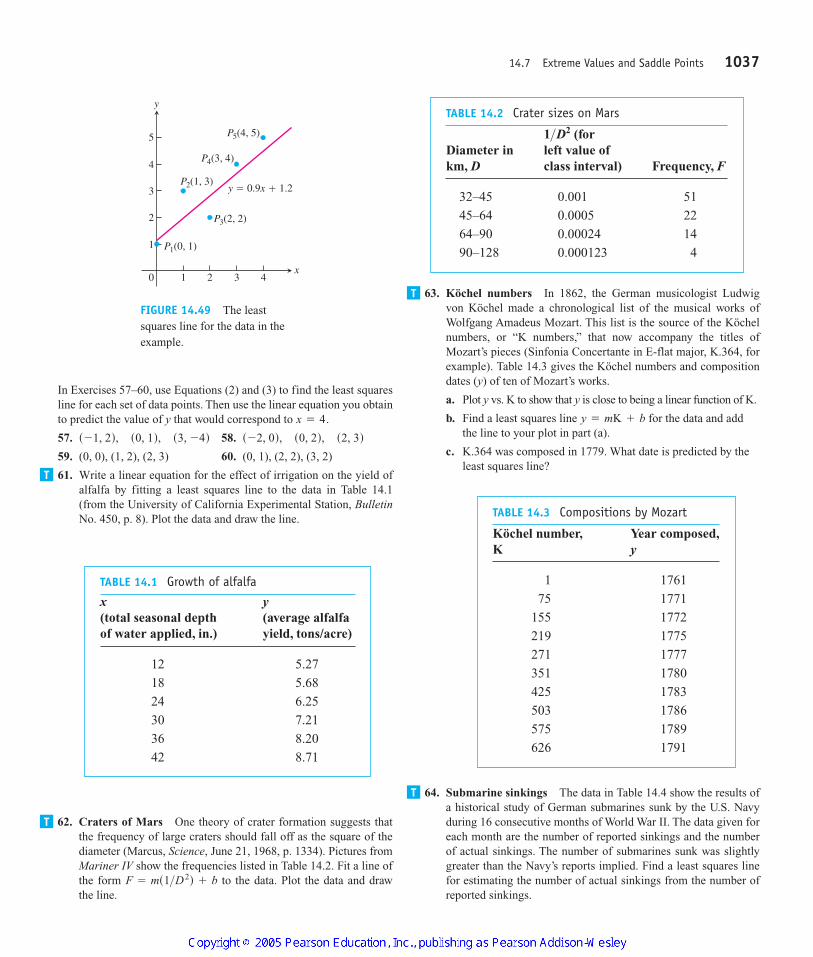
In Exercises 57–60, use Equations (2) and (3) to find the least squaresline for each set of data points. Then use the linear equation you obtainto predict the value of y that would correspond to
57. 58.
59. (0, 0), (1, 2), (2, 3) 60. (0, 1), (2, 2), (3, 2)
61. Write a linear equation for the effect of irrigation on the yield ofalfalfa by fitting a least squares line to the data in Table 14.1(from the University of California Experimental Station, BulletinNo. 450, p. 8). Plot the data and draw the line.
s -2, 0d, s0, 2d, s2, 3ds -1, 2d, s0, 1d, s3, -4dx = 4.
63. Köchel numbers In 1862, the German musicologist Ludwigvon Köchel made a chronological list of the musical works ofWolfgang Amadeus Mozart. This list is the source of the Köchelnumbers, or “K numbers,” that now accompany the titles ofMozart’s pieces (Sinfonia Concertante in E-flat major, K.364, forexample). Table 14.3 gives the Köchel numbers and compositiondates (y) of ten of Mozart’s works.
a. Plot y vs. K to show that y is close to being a linear function of K.
b. Find a least squares line for the data and addthe line to your plot in part (a).
c. K.364 was composed in 1779. What date is predicted by theleast squares line?
y = mK + b
14.7 Extreme Values and Saddle Points 1037
x
y
0 1 2 3 4
1
2
3
4
5
P1(0, 1)
P3(2, 2)
P2(1, 3)
P4(3, 4)
P5(4, 5)
y � 0.9x � 1.2
FIGURE 14.49 The leastsquares line for the data in theexample.
TABLE 14.1 Growth of alfalfa
x y(total seasonal depth (average alfalfaof water applied, in.) yield, tons/acre)
12 5.27
18 5.68
24 6.25
30 7.21
36 8.20
42 8.71
TABLE 14.2 Crater sizes on Mars
(forDiameter in left value ofkm, D class interval) Frequency, F
32–45 0.001 51
45–64 0.0005 22
64–90 0.00024 14
90–128 0.000123 4
1>D2
T
T
TABLE 14.3 Compositions by Mozart
Köchel number, Year composed,K y
1 1761
75 1771
155 1772
219 1775
271 1777
351 1780
425 1783
503 1786
575 1789
626 1791
T
T
62. Craters of Mars One theory of crater formation suggests thatthe frequency of large craters should fall off as the square of thediameter (Marcus, Science, June 21, 1968, p. 1334). Pictures fromMariner IV show the frequencies listed in Table 14.2. Fit a line ofthe form to the data. Plot the data and drawthe line.
F = ms1>D2d + b
64. Submarine sinkings The data in Table 14.4 show the results ofa historical study of German submarines sunk by the U.S. Navyduring 16 consecutive months of World War II. The data given foreach month are the number of reported sinkings and the numberof actual sinkings. The number of submarines sunk was slightlygreater than the Navy’s reports implied. Find a least squares linefor estimating the number of actual sinkings from the number ofreported sinkings.
4100 AWL/Thomas_ch14p965-1066 8/25/04 2:53 PM Page 1037
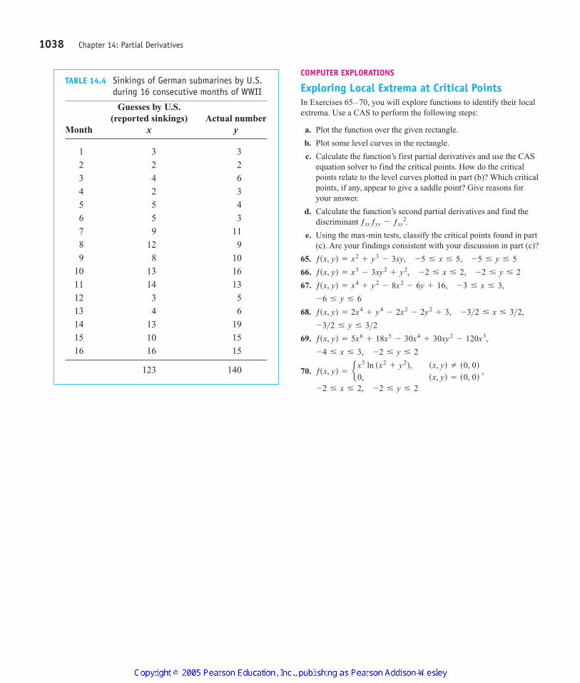
COMPUTER EXPLORATIONS
Exploring Local Extrema at Critical PointsIn Exercises 65–70, you will explore functions to identify their localextrema. Use a CAS to perform the following steps:
a. Plot the function over the given rectangle.
b. Plot some level curves in the rectangle.
c. Calculate the function’s first partial derivatives and use the CASequation solver to find the critical points. How do the criticalpoints relate to the level curves plotted in part (b)? Which criticalpoints, if any, appear to give a saddle point? Give reasons foryour answer.
d. Calculate the function’s second partial derivatives and find thediscriminant
e. Using the max-min tests, classify the critical points found in part(c). Are your findings consistent with your discussion in part (c)?
65.
66.
67.
68.
69.
70.
-2 … x … 2, -2 … y … 2
ƒsx, yd = e x5 ln sx2+ y2d, sx, yd Z s0, 0d
0, sx, yd = s0, 0d ,
-4 … x … 3, -2 … y … 2
ƒsx, yd = 5x6+ 18x5
- 30x4+ 30xy2
- 120x3,
-3>2 … y … 3>2ƒsx, yd = 2x4
+ y4- 2x2
- 2y2+ 3, -3>2 … x … 3>2,
-6 … y … 6
ƒsx, yd = x4+ y2
- 8x2- 6y + 16, -3 … x … 3,
ƒsx, yd = x3- 3xy2
+ y2, -2 … x … 2, -2 … y … 2
ƒsx, yd = x2+ y3
- 3xy, -5 … x … 5, -5 … y … 5
ƒxx ƒyy - ƒxy2.
1038 Chapter 14: Partial Derivatives
TABLE 14.4 Sinkings of German submarines by U.S.during 16 consecutive months of WWII
Guesses by U.S.(reported sinkings) Actual number
Month x y
1 3 3
2 2 2
3 4 6
4 2 3
5 5 4
6 5 3
7 9 11
8 12 9
9 8 10
10 13 16
11 14 13
12 3 5
13 4 6
14 13 19
15 10 15
16 16 15
123 140
4100 AWL/Thomas_ch14p965-1066 8/25/04 2:53 PM Page 1038
1038 Chapter 14: Partial Derivatives
Lagrange Multipliers
Sometimes we need to find the extreme values of a function whose domain is constrainedto lie within some particular subset of the plane—a disk, for example, a closed triangularregion, or along a curve. In this section, we explore a powerful method for finding extremevalues of constrained functions: the method of Lagrange multipliers.
Constrained Maxima and Minima
EXAMPLE 1 Finding a Minimum with Constraint
Find the point P(x, y, z) closest to the origin on the plane
Solution The problem asks us to find the minimum value of the function
= 2x2+ y2
+ z2
ƒ OP1
ƒ = 2sx - 0d2+ s y - 0d2
+ sz - 0d2
2x + y - z - 5 = 0.
14.8
HISTORICAL BIOGRAPHY
Joseph Louis Lagrange(1736–1813)
4100 AWL/Thomas_ch14p965-1066 8/25/04 2:53 PM Page 1038
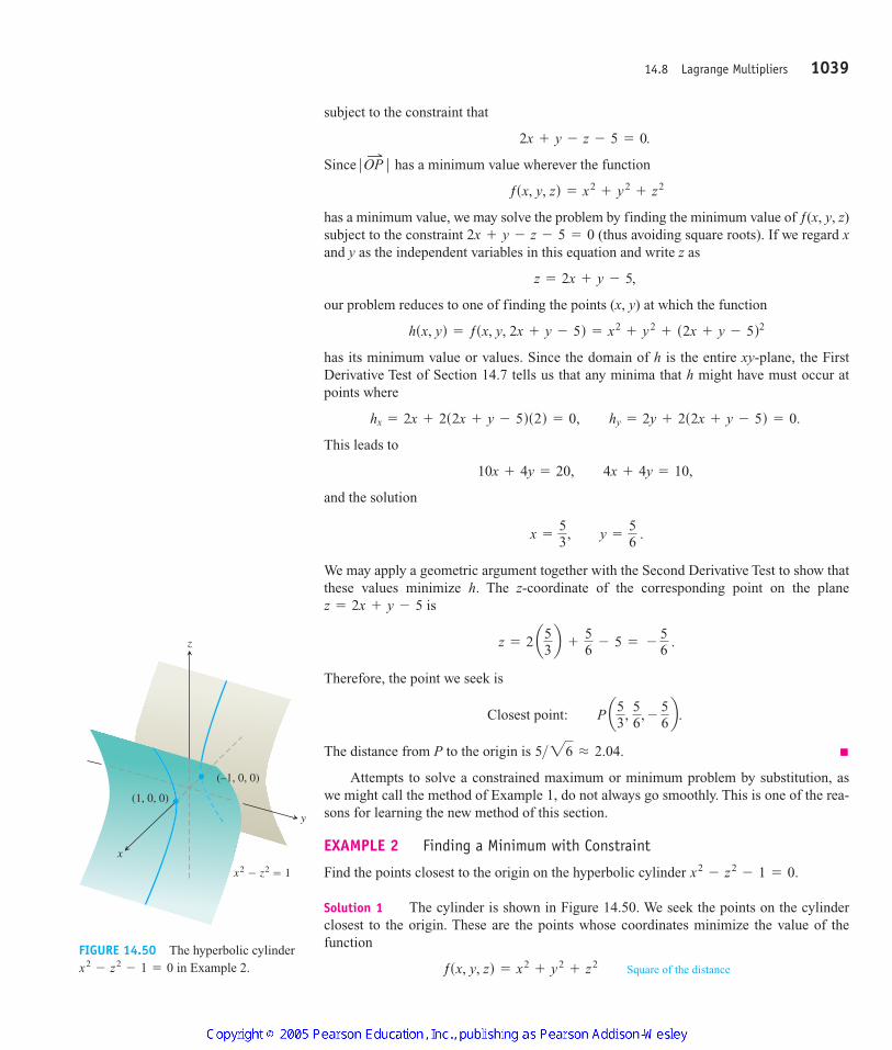
subject to the constraint that
Since has a minimum value wherever the function
has a minimum value, we may solve the problem by finding the minimum value of ƒ(x, y, z)subject to the constraint (thus avoiding square roots). If we regard xand y as the independent variables in this equation and write z as
our problem reduces to one of finding the points (x, y) at which the function
has its minimum value or values. Since the domain of h is the entire xy-plane, the FirstDerivative Test of Section 14.7 tells us that any minima that h might have must occur atpoints where
This leads to
and the solution
We may apply a geometric argument together with the Second Derivative Test to show thatthese values minimize h. The z-coordinate of the corresponding point on the plane
is
Therefore, the point we seek is
The distance from P to the origin is
Attempts to solve a constrained maximum or minimum problem by substitution, aswe might call the method of Example 1, do not always go smoothly. This is one of the rea-sons for learning the new method of this section.
EXAMPLE 2 Finding a Minimum with Constraint
Find the points closest to the origin on the hyperbolic cylinder
Solution 1 The cylinder is shown in Figure 14.50. We seek the points on the cylinderclosest to the origin. These are the points whose coordinates minimize the value of thefunction
Square of the distanceƒsx, y, zd = x2+ y2
+ z2
x2- z2
- 1 = 0.
5>26 L 2.04.
Closest point: P a53
, 56
, -56b.
z = 2 a53b +
56
- 5 = -56
.
z = 2x + y - 5
x =
53
, y =
56
.
10x + 4y = 20, 4x + 4y = 10,
hx = 2x + 2s2x + y - 5ds2d = 0, hy = 2y + 2s2x + y - 5d = 0.
hsx, yd = ƒsx, y, 2x + y - 5d = x2+ y2
+ s2x + y - 5d2
z = 2x + y - 5,
2x + y - z - 5 = 0
ƒsx, y, zd = x2+ y2
+ z2
ƒ OP1
ƒ
2x + y - z - 5 = 0.
14.8 Lagrange Multipliers 1039
(1, 0, 0)
z
y
x
x2 � z2 � 1
(–1, 0, 0)
FIGURE 14.50 The hyperbolic cylinderin Example 2.x2
- z2- 1 = 0
4100 AWL/Thomas_ch14p965-1066 8/25/04 2:53 PM Page 1039
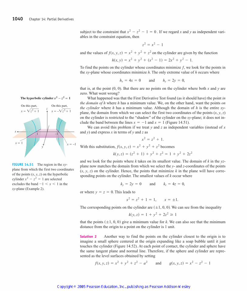
subject to the constraint that If we regard x and y as independent vari-ables in the constraint equation, then
and the values of on the cylinder are given by the function
To find the points on the cylinder whose coordinates minimize ƒ, we look for the points inthe xy-plane whose coordinates minimize h. The only extreme value of h occurs where
that is, at the point (0, 0). But there are no points on the cylinder where both x and y arezero. What went wrong?
What happened was that the First Derivative Test found (as it should have) the point inthe domain of h where h has a minimum value. We, on the other hand, want the points onthe cylinder where h has a minimum value. Although the domain of h is the entire xy-plane, the domain from which we can select the first two coordinates of the points (x, y, z)on the cylinder is restricted to the “shadow” of the cylinder on the xy-plane; it does not in-clude the band between the lines and (Figure 14.51).
We can avoid this problem if we treat y and z as independent variables (instead of xand y) and express x in terms of y and z as
With this substitution, becomes
and we look for the points where k takes on its smallest value. The domain of k in the yz-plane now matches the domain from which we select the y- and z-coordinates of the points(x, y, z) on the cylinder. Hence, the points that minimize k in the plane will have corre-sponding points on the cylinder. The smallest values of k occur where
or where This leads to
The corresponding points on the cylinder are We can see from the inequality
that the points give a minimum value for k. We can also see that the minimumdistance from the origin to a point on the cylinder is 1 unit.
Solution 2 Another way to find the points on the cylinder closest to the origin is toimagine a small sphere centered at the origin expanding like a soap bubble until it justtouches the cylinder (Figure 14.52). At each point of contact, the cylinder and sphere havethe same tangent plane and normal line. Therefore, if the sphere and cylinder are repre-sented as the level surfaces obtained by setting
ƒsx, y, zd = x2+ y2
+ z2- a2 and gsx, y, zd = x2
- z2- 1
s ;1, 0, 0d
ks y, zd = 1 + y2+ 2z2
Ú 1
s ;1, 0, 0d.
x2= z2
+ 1 = 1, x = ;1.
y = z = 0.
ky = 2y = 0 and kz = 4z = 0,
ks y, zd = sz2+ 1d + y2
+ z2= 1 + y2
+ 2z2
ƒsx, y, zd = x2+ y2
+ z2
x2= z2
+ 1.
x = 1x = -1
hx = 4x = 0 and hy = 2y = 0,
hsx, yd = x2+ y2
+ sx2- 1d = 2x2
+ y2- 1.
ƒsx, y, zd = x2+ y2
+ z2
z2= x2
- 1
x2- z2
- 1 = 0 .
1040 Chapter 14: Partial Derivatives
On this part, On this part,
x � �z2 � 1
x
z
–11
yx � –1x � 1
The hyperbolic cylinder x2 � z2 � 1
x � –�z2 � 1
FIGURE 14.51 The region in the xy-plane from which the first two coordinatesof the points (x, y, z) on the hyperboliccylinder are selectedexcludes the band in thexy-plane (Example 2).
-1 6 x 6 1x2
- z2= 1
4100 AWL/Thomas_ch14p965-1066 8/25/04 2:53 PM Page 1040
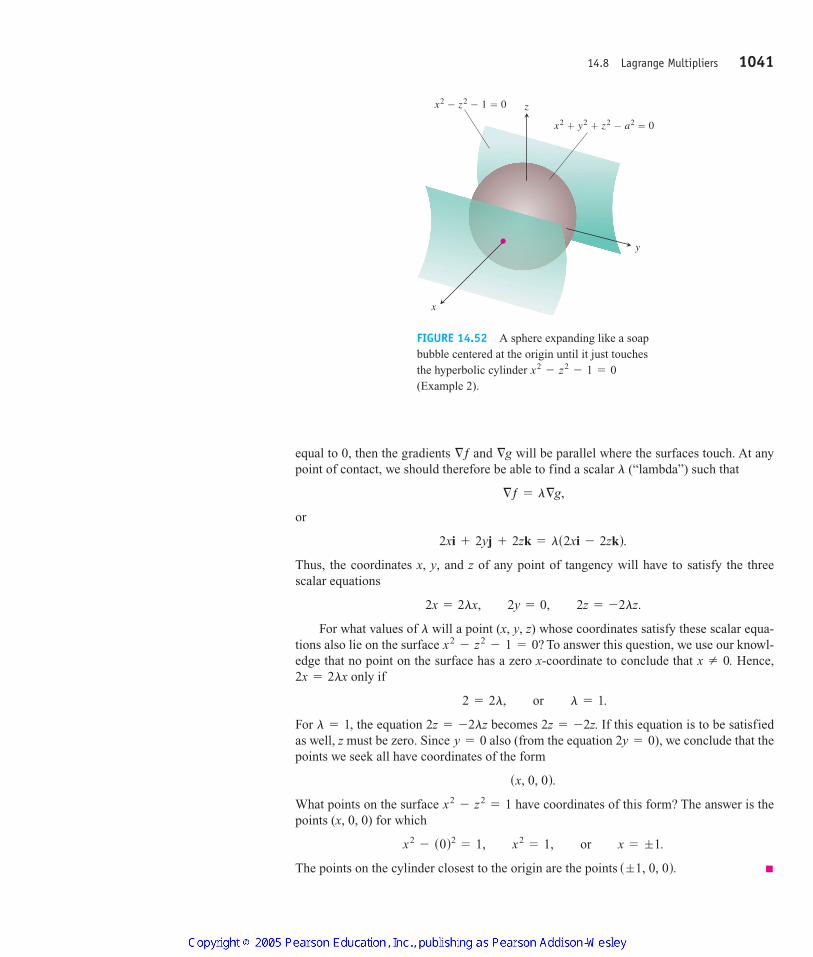
equal to 0, then the gradients and will be parallel where the surfaces touch. At anypoint of contact, we should therefore be able to find a scalar (“lambda”) such that
or
Thus, the coordinates x, y, and z of any point of tangency will have to satisfy the threescalar equations
For what values of will a point (x, y, z) whose coordinates satisfy these scalar equa-tions also lie on the surface To answer this question, we use our knowl-edge that no point on the surface has a zero x-coordinate to conclude that Hence,
only if
For the equation becomes If this equation is to be satisfiedas well, z must be zero. Since also (from the equation ), we conclude that thepoints we seek all have coordinates of the form
What points on the surface have coordinates of this form? The answer is thepoints (x, 0, 0) for which
The points on the cylinder closest to the origin are the points s ;1, 0, 0d.
x2- s0d2
= 1, x2= 1, or x = ;1.
x2- z2
= 1
sx, 0, 0d.
2y = 0y = 02z = -2z.2z = -2lzl = 1,
2 = 2l, or l = 1.
2x = 2lxx Z 0.
x2- z2
- 1 = 0?l
2x = 2lx, 2y = 0, 2z = -2lz.
2xi + 2yj + 2zk = ls2xi - 2zkd.
§ƒ = l§g,
l
§g§ƒ
14.8 Lagrange Multipliers 1041
z
y
x
x2 � y2 � z2 � a2 � 0
x2 � z2 � 1 � 0
FIGURE 14.52 A sphere expanding like a soapbubble centered at the origin until it just touchesthe hyperbolic cylinder (Example 2).
x2- z2
- 1 = 0
4100 AWL/Thomas_ch14p965-1066 9/2/04 11:09 AM Page 1041
The Method of Lagrange Multipliers
In Solution 2 of Example 2, we used the method of Lagrange multipliers. The methodsays that the extreme values of a function ƒ(x, y, z) whose variables are subject to a con-straint are to be found on the surface at the points where
for some scalar (called a Lagrange multiplier).To explore the method further and see why it works, we first make the following ob-
servation, which we state as a theorem.
l
§ƒ = l§g
g = 0gsx, y, zd = 0
1042 Chapter 14: Partial Derivatives
THEOREM 12 The Orthogonal Gradient TheoremSuppose that ƒ(x, y, z) is differentiable in a region whose interior contains asmooth curve
If is a point on C where ƒ has a local maximum or minimum relative to its val-ues on C, then is orthogonal to C at P0 .§ƒ
P0
C: rstd = gstdi + hstdj + kstdk.
COROLLARY OF THEOREM 12At the points on a smooth curve where a differentiable func-tion ƒ(x, y) takes on its local maxima and minima relative to its values on thecurve, , where v = dr>dt.§ƒ # v = 0
rstd = gstdi + hstdj
Proof We show that is orthogonal to the curve’s velocity vector at The values of ƒon C are given by the composite ƒ(g(t), h(t), k(t)), whose derivative with respect to t is
At any point where ƒ has a local maximum or minimum relative to its values on thecurve, so
By dropping the z-terms in Theorem 12, we obtain a similar result for functions of twovariables.
§ƒ # v = 0.
dƒ>dt = 0,P0
dƒdt
=
0ƒ0x
dgdt
+
0ƒ0y
dhdt
+
0ƒ0z
dkdt
= §ƒ # v.
P0 .§ƒ
Theorem 12 is the key to the method of Lagrange multipliers. Suppose that ƒ(x, y, z)and g(x, y, z) are differentiable and that is a point on the surface where ƒhas a local maximum or minimum value relative to its other values on the surface. Then ƒtakes on a local maximum or minimum at relative to its values on every differentiablecurve through on the surface Therefore, is orthogonal to the velocityvector of every such differentiable curve through So is moreover (because isorthogonal to the level surface as we saw in Section 14.5). Therefore, at issome scalar multiple of §g.l
P0, §ƒg = 0,§g§g ,P0 .
§ƒgsx, y, zd = 0.P0
P0
gsx, y, zd = 0P0
4100 AWL/Thomas_ch14p965-1066 8/25/04 2:53 PM Page 1042
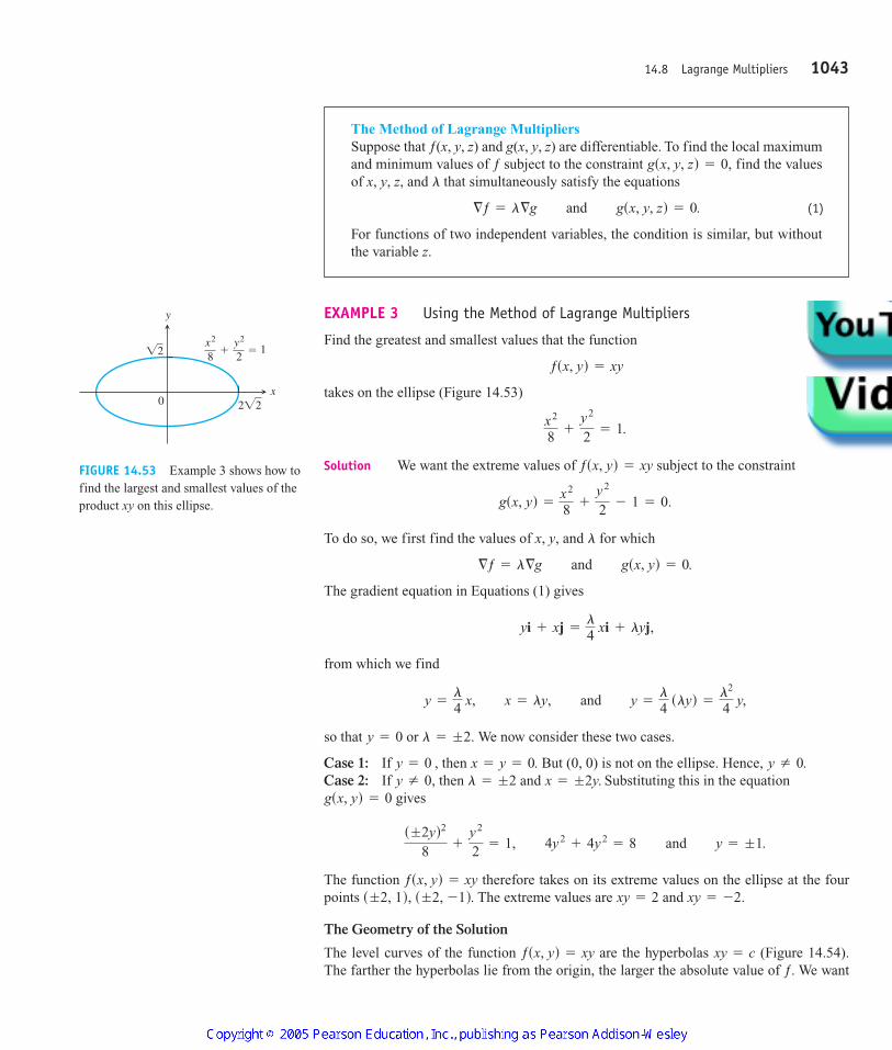
EXAMPLE 3 Using the Method of Lagrange Multipliers
Find the greatest and smallest values that the function
takes on the ellipse (Figure 14.53)
Solution We want the extreme values of subject to the constraint
To do so, we first find the values of x, y, and for which
The gradient equation in Equations (1) gives
from which we find
so that or We now consider these two cases.
Case 1: If then But (0, 0) is not on the ellipse. Hence, Case 2: If then and Substituting this in the equation
gives
The function therefore takes on its extreme values on the ellipse at the fourpoints The extreme values are and
The Geometry of the Solution
The level curves of the function are the hyperbolas (Figure 14.54).The farther the hyperbolas lie from the origin, the larger the absolute value of ƒ. We want
xy = cƒsx, yd = xy
xy = -2.xy = 2s ;2, 1d, s ;2, -1d.ƒsx, yd = xy
s ;2yd2
8+
y2
2= 1, 4y2
+ 4y2= 8 and y = ;1.
gsx, yd = 0x = ;2y.l = ;2y Z 0,
y Z 0.x = y = 0.y = 0 ,
l = ;2.y = 0
y =
l4
x, x = ly, and y =
l4
slyd =
l2
4 y,
yi + xj =
l4
xi + lyj,
§ƒ = l§g and gsx, yd = 0.
l
gsx, yd =
x2
8+
y2
2- 1 = 0.
ƒsx, yd = xy
x2
8+
y2
2= 1.
ƒsx, yd = xy
14.8 Lagrange Multipliers 1043
The Method of Lagrange MultipliersSuppose that ƒ(x, y, z) and g(x, y, z) are differentiable. To find the local maximumand minimum values of ƒ subject to the constraint find the valuesof x, y, z, and that simultaneously satisfy the equations
(1)
For functions of two independent variables, the condition is similar, but withoutthe variable z.
§ƒ = l§g and gsx, y, zd = 0.
l
gsx, y, zd = 0,
y
x0 2�2
�2 � � 1x2
8y2
2
FIGURE 14.53 Example 3 shows how tofind the largest and smallest values of theproduct xy on this ellipse.
4100 AWL/Thomas_ch14p965-1066 8/25/04 2:53 PM Page 1043
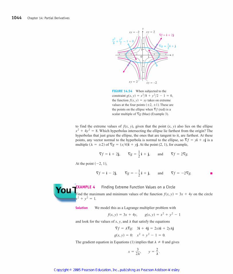
to find the extreme values of ƒ(x, y), given that the point (x, y) also lies on the ellipseWhich hyperbolas intersecting the ellipse lie farthest from the origin? The
hyperbolas that just graze the ellipse, the ones that are tangent to it, are farthest. At thesepoints, any vector normal to the hyperbola is normal to the ellipse, so is amultiple of At the point (2, 1), for example,
At the point
EXAMPLE 4 Finding Extreme Function Values on a Circle
Find the maximum and minimum values of the function on the circle
Solution We model this as a Lagrange multiplier problem with
and look for the values of x, y, and that satisfy the equations
The gradient equation in Equations (1) implies that and gives
x =
32l
, y =2l
.
l Z 0
gsx, yd = 0: x2+ y2
- 1 = 0.
§ƒ = l§g: 3i + 4j = 2xli + 2ylj
l
ƒsx, yd = 3x + 4y, gsx, yd = x2+ y2
- 1
x2+ y2
= 1.ƒsx, yd = 3x + 4y
§ƒ = i - 2j, §g = -12
i + j, and §ƒ = -2§g.
s -2, 1d,
§ƒ = i + 2j, §g =12
i + j, and §ƒ = 2§g.
§g = sx>4di + yj.sl = ;2d§ƒ = yi + xj
x2+ 4y2
= 8.
1044 Chapter 14: Partial Derivatives
y
x0 1
1
xy � –2∇f � i � 2j
xy � 2
∇g � i � j12
xy � –2xy � 2
� � 1 � 02y2
8x2
FIGURE 14.54 When subjected to theconstraint the function takes on extremevalues at the four points These arethe points on the ellipse when (red) is ascalar multiple of (blue) (Example 3).§g
§ƒs ;2, ;1d.
ƒsx, yd = xygsx, yd = x2>8 + y2>2 - 1 = 0,
4100 AWL/Thomas_ch14p965-1066 8/25/04 2:53 PM Page 1044
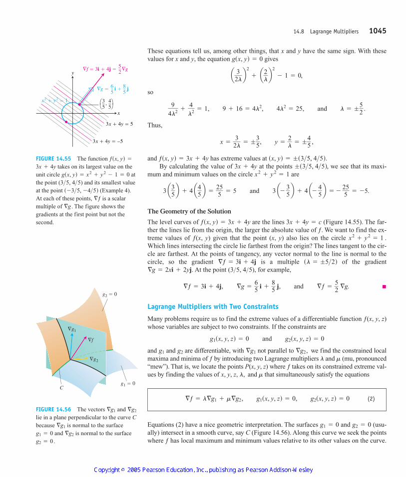
These equations tell us, among other things, that x and y have the same sign. With thesevalues for x and y, the equation gives
so
Thus,
and has extreme values at By calculating the value of at the points we see that its maxi-
mum and minimum values on the circle are
The Geometry of the Solution
The level curves of are the lines (Figure 14.55). The far-ther the lines lie from the origin, the larger the absolute value of ƒ. We want to find the ex-treme values of ƒ(x, y) given that the point (x, y) also lies on the circle Which lines intersecting the circle lie farthest from the origin? The lines tangent to the cir-cle are farthest. At the points of tangency, any vector normal to the line is normal to thecircle, so the gradient is a multiple of the gradient
At the point (3 5, 4 5), for example,
Lagrange Multipliers with Two Constraints
Many problems require us to find the extreme values of a differentiable function ƒ(x, y, z)whose variables are subject to two constraints. If the constraints are
and and are differentiable, with not parallel to we find the constrained localmaxima and minima of ƒ by introducing two Lagrange multipliers and (mu, pronounced“mew”). That is, we locate the points P(x, y, z) where ƒ takes on its constrained extreme val-ues by finding the values of and that simultaneously satisfy the equationsmx, y, z, l,
ml
§g2,§g1g2g1
g1sx, y, zd = 0 and g2sx, y, zd = 0
§ƒ = 3i + 4j, §g =
65 i +
85 j, and §ƒ =
52
§g.
>>§g = 2xi + 2yj.sl = ;5>2d§ƒ = 3i + 4j
x2+ y2
= 1 .
3x + 4y = cƒsx, yd = 3x + 4y
3 a35 b + 4 a45 b =
255 = 5 and 3 a- 3
5 b + 4 a- 45 b = -
255 = -5.
x2+ y2
= 1;s3>5, 4>5d,3x + 4y
sx, yd = ;s3>5, 4>5d.ƒsx, yd = 3x + 4y
x =
32l
= ;
35, y =
2l
= ;45 ,
94l2 +
4l2 = 1, 9 + 16 = 4l2, 4l2
= 25, and l = ;
52
.
a 32lb2
+ a2lb2
- 1 = 0,
gsx, yd = 0
14.8 Lagrange Multipliers 1045
y
x
3x � 4y � 5
3x � 4y � –5
x2 � y2 � 1
35
45
,
∇f � 3i � 4j � ∇g52
∇g � i � j65
85
FIGURE 14.55 The function takes on its largest value on the
unit circle atthe point (3 5, 4 5) and its smallest valueat the point (Example 4). At each of these points, is a scalarmultiple of The figure shows thegradients at the first point but not thesecond.
§g .§ƒ
s -3>5, -4>5d>>
gsx, yd = x2+ y2
- 1 = 03x + 4y
ƒsx, yd =
C
g2 � 0
g1 � 0
∇f
∇g2
∇g1
FIGURE 14.56 The vectors and lie in a plane perpendicular to the curve Cbecause is normal to the surface
and is normal to the surfaceg2 = 0.
§g2g1 = 0§g1
§g2§g1
(2)§ƒ = l§g1 + m§g2, g1sx, y, zd = 0, g2sx, y, zd = 0
Equations (2) have a nice geometric interpretation. The surfaces and (usu-ally) intersect in a smooth curve, say C (Figure 14.56). Along this curve we seek the pointswhere ƒ has local maximum and minimum values relative to its other values on the curve.
g2 = 0g1 = 0
4100 AWL/Thomas_ch14p965-1066 9/2/04 11:09 AM Page 1045
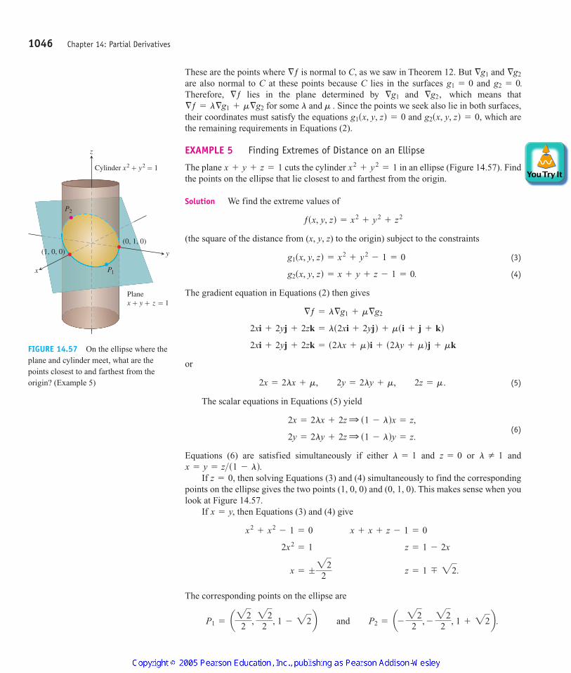
These are the points where is normal to C, as we saw in Theorem 12. But and are also normal to C at these points because C lies in the surfaces and Therefore, lies in the plane determined by and which means that
for some and Since the points we seek also lie in both surfaces,their coordinates must satisfy the equations and which arethe remaining requirements in Equations (2).
EXAMPLE 5 Finding Extremes of Distance on an Ellipse
The plane cuts the cylinder in an ellipse (Figure 14.57). Findthe points on the ellipse that lie closest to and farthest from the origin.
Solution We find the extreme values of
(the square of the distance from (x, y, z) to the origin) subject to the constraints
(3)
(4)
The gradient equation in Equations (2) then gives
or
(5)
The scalar equations in Equations (5) yield
(6)
Equations (6) are satisfied simultaneously if either and or and
If then solving Equations (3) and (4) simultaneously to find the correspondingpoints on the ellipse gives the two points (1, 0, 0) and (0, 1, 0). This makes sense when youlook at Figure 14.57.
If then Equations (3) and (4) give
The corresponding points on the ellipse are
P1 = a222
, 222
, 1 - 22b and P2 = a- 222
, -222
, 1 + 22b.
x = ;
222 z = 1 < 22.
2x2= 1 z = 1 - 2x
x2+ x2
- 1 = 0 x + x + z - 1 = 0
x = y,
z = 0,x = y = z>s1 - ld.
l Z 1z = 0l = 1
2y = 2ly + 2z Q s1 - ldy = z.
2x = 2lx + 2z Q s1 - ldx = z,
2x = 2lx + m, 2y = 2ly + m, 2z = m.
2xi + 2yj + 2zk = s2lx + mdi + s2ly + mdj + mk
2xi + 2yj + 2zk = ls2xi + 2yjd + msi + j + kd
§ƒ = l§g1 + m§g2
g2sx, y, zd = x + y + z - 1 = 0.
g1sx, y, zd = x2+ y2
- 1 = 0
ƒsx, y, zd = x2+ y2
+ z2
x2+ y2
= 1x + y + z = 1
g2sx, y, zd = 0,g1sx, y, zd = 0m .l§ƒ = l§g1 + m§g2
§g2,§g1§ƒg2 = 0.g1 = 0
§g2§g1§ƒ
1046 Chapter 14: Partial Derivatives
Cylinder x2 � y2 � 1
Planex � y � z � 1
z
(0, 1, 0)(1, 0, 0) y
x P1
P2
FIGURE 14.57 On the ellipse where theplane and cylinder meet, what are thepoints closest to and farthest from theorigin? (Example 5)
4100 AWL/Thomas_ch14p965-1066 9/2/04 11:09 AM Page 1046
Here we need to be careful, however. Although and both give local maxima of ƒ onthe ellipse, is farther from the origin than
The points on the ellipse closest to the origin are (1, 0, 0) and (0, 1, 0). The point onthe ellipse farthest from the origin is P2.
P1.P2
P2P1
14.8 Lagrange Multipliers 1047
4100 AWL/Thomas_ch14p965-1066 8/25/04 2:53 PM Page 1047
14.8 Lagrange Multipliers 1047
EXERCISES 14.8
Two Independent Variables with One Constraint1. Extrema on an ellipse Find the points on the ellipse
where as its extreme values.
2. Extrema on a circle Find the extreme values of subject to the constraint
3. Maximum on a line Find the maximum value of on the line .
4. Extrema on a line Find the local extreme values ofon the line
5. Constrained minimum Find the points on the curve nearest the origin.
6. Constrained minimum Find the points on the curve nearest the origin.
7. Use the method of Lagrange multipliers to find
a. Minimum on a hyperbola The minimum value of subject to the constraints
b. Maximum on a line The maximum value of xy, subject tothe constraint
Comment on the geometry of each solution.
8. Extrema on a curve Find the points on the curve in the xy-plane that are nearest to and farthest from the
origin.
9. Minimum surface area with fixed volume Find the dimen-sions of the closed right circular cylindrical can of smallest sur-face area whose volume is
10. Cylinder in a sphere Find the radius and height of the openright circular cylinder of largest surface area that can be inscribedin a sphere of radius a. What is the largest surface area?
11. Rectangle of greatest area in an ellipse Use the method ofLagrange multipliers to find the dimensions of the rectangle of greatest area that can be inscribed in the ellipse
with sides parallel to the coordinate axes.
12. Rectangle of longest perimeter in an ellipse Find the dimen-sions of the rectangle of largest perimeter that can be inscribed inthe ellipse with sides parallel to the coordi-nate axes. What is the largest perimeter?
13. Extrema on a circle Find the maximum and minimum valuesof subject to the constraint
14. Extrema on a circle Find the maximum and minimum valuesof subject to the constraint x2
+ y2= 4.3x - y + 6
x2- 2x + y2
- 4y = 0.x2+ y2
x2>a2+ y2>b2
= 1
x2>16 + y2>9 = 1
16p cm3 .
y2= 1
x2+ xy +
x + y = 16.
xy = 16, x 7 0, y 7 0x + y,
x2y = 2
xy2= 54
x + y = 3 .ƒsx, yd = x2y
x + 3y = 1049 - x2- y2
ƒsx, yd =
gsx, yd = x2+ y2
- 10 = 0.ƒsx, yd = xy
ƒsx, yd = xyx2+ 2y2
= 1
15. Ant on a metal plate The temperature at a point (x, y) on ametal plate is An ant on the platewalks around the circle of radius 5 centered at the origin. Whatare the highest and lowest temperatures encountered by the ant?
16. Cheapest storage tank Your firm has been asked to design astorage tank for liquid petroleum gas. The customer’s specifica-tions call for a cylindrical tank with hemispherical ends, and thetank is to hold of gas. The customer also wants to use thesmallest amount of material possible in building the tank. Whatradius and height do you recommend for the cylindrical portionof the tank?
Three Independent Variableswith One Constraint17. Minimum distance to a point Find the point on the plane
closest to the point (1, 1, 1).
18. Maximum distance to a point Find the point on the spherefarthest from the point
19. Minimum distance to the origin Find the minimum distancefrom the surface to the origin.
20. Minimum distance to the origin Find the point on the surfacenearest the origin.
21. Minimum distance to the origin Find the points on the surfaceclosest to the origin.
22. Minimum distance to the origin Find the point(s) on the sur-face closest to the origin.
23. Extrema on a sphere Find the maximum and minimum values of
on the sphere
24. Extrema on a sphere Find the points on the spherewhere has its
maximum and minimum values.
25. Minimizing a sum of squares Find three real numbers whosesum is 9 and the sum of whose squares is as small as possible.
26. Maximizing a product Find the largest product the positivenumbers x, y, and z can have if
27. Rectangular box of longest volume in a sphere Find the di-mensions of the closed rectangular box with maximum volumethat can be inscribed in the unit sphere.
x + y + z2= 16.
ƒsx, y, zd = x + 2y + 3zx2+ y2
+ z2= 25
x2+ y2
+ z2= 30.
ƒsx, y, zd = x - 2y + 5z
xyz = 1
z2= xy + 4
z = xy + 1
x2+ y2
- z2= 1
s1, -1, 1d .x2+ y2
+ z2= 4
x + 2y + 3z = 13
8000 m3
Tsx, yd = 4x2- 4xy + y2.
4100 AWL/Thomas_ch14p965-1066 8/25/04 2:53 PM Page 1047
28. Box with vertex on a plane Find the volume of the largestclosed rectangular box in the first octant having three faces in the coordinate planes and a vertex on the plane
where and
29. Hottest point on a space probe A space probe in the shape ofthe ellipsoid
enters Earth’s atmosphere and its surface begins to heat. After 1hour, the temperature at the point (x, y, z) on the probe’s surface is
Find the hottest point on the probe’s surface.
30. Extreme temperatures on a sphere Suppose that the Celsiustemperature at the point (x, y, z) on the sphere is Locate the highest and lowest temperatures onthe sphere.
31. Maximizing a utility function: an example from economicsIn economics, the usefulness or utility of amounts x and y of twocapital goods and is sometimes measured by a functionU(x, y). For example, and might be two chemicals a phar-maceutical company needs to have on hand and U(x, y) the gainfrom manufacturing a product whose synthesis requires differentamounts of the chemicals depending on the process used. If costs a dollars per kilogram, costs b dollars per kilogram, andthe total amount allocated for the purchase of and togetheris c dollars, then the company’s managers want to maximizeU(x, y) given that Thus, they need to solve a typi-cal Lagrange multiplier problem.
Suppose that
and that the equation simplifies to
Find the maximum value of U and the corresponding values of xand y subject to this latter constraint.
32. Locating a radio telescope You are in charge of erecting a ra-dio telescope on a newly discovered planet. To minimize interfer-ence, you want to place it where the magnetic field of the planet isweakest. The planet is spherical, with a radius of 6 units. Basedon a coordinate system whose origin is at the center of the planet,the strength of the magnetic field is given by
Where should you locate the radio tele-scope?
Extreme Values Subject to Two Constraints33. Maximize the function subject to the
constraints and
34. Minimize the function subject to theconstraints and x + 3y + 9z = 9.x + 2y + 3z = 6
ƒsx, y, zd = x2+ y2
+ z2
y + z = 0.2x - y = 0ƒsx, y, zd = x2
+ 2y - z2
6x - y2+ xz + 60.
Msx, y, zd =
2x + y = 30.
ax + by = c
Usx, yd = xy + 2x
ax + by = c .
G2G1
G2
G1
G2G1
G2G1
T = 400xyz2 .x2
+ y2+ z2
= 1
Tsx, y, zd = 8x2+ 4yz - 16z + 600 .
4x2+ y2
+ 4z2= 16
c 7 0.a 7 0, b 7 0,x>a + y>b + z>c = 1,
35. Minimum distance to the origin Find the point closest to theorigin on the line of intersection of the planes and
36. Maximum value on line of intersection Find the maximumvalue that can have on the line of in-tersection of the planes and
37. Extrema on a curve of intersection Find the extreme values ofon the intersection of the plane with
the sphere
38. a. Maximum on line of intersection Find the maximum valueof on the line of intersection of the two planes
and
b. Give a geometric argument to support your claim that youhave found a maximum, and not a minimum, value of w.
39. Extrema on a circle of intersection Find the extreme values ofthe function on the circle in which the plane
intersects the sphere
40. Minimum distance to the origin Find the point closest to theorigin on the curve of intersection of the plane andthe cone
Theory and Examples41. The condition is not sufficient Although
is a necessary condition for the occurrence of an extreme value ofƒ(x, y) subject to the condition it does not in itselfguarantee that one exists. As a case in point, try using the methodof Lagrange multipliers to find a maximum value of
subject to the constraint that Themethod will identify the two points (4, 4) and as candi-dates for the location of extreme values. Yet the sum hasno maximum value on the hyperbola The farther you gofrom the origin on this hyperbola in the first quadrant, the largerthe sum becomes.
42. A least squares plane The plane is to be“fitted” to the following points
Find the values of A, B, and C that minimize
the sum of the squares of the deviations.
43. a. Maximum on a sphere Show that the maximum value ofon a sphere of radius r centered at the origin of a
Cartesian abc-coordinate system is
b. Geometric and arithmetic means Using part (a), showthat for nonnegative numbers a, b, and c,
that is, the geometric mean of three nonnegative numbers isless than or equal to their arithmetic mean.
sabcd1>3…
a + b + c3
;
sr2>3d3.a2b2c2
a4
k = 1sAxk + Byk + C - zkd2 ,
s0, 0, 0d, s0, 1, 1d, s1, 1, 1d, s1, 0, -1d.
sxk, yk, zkd:z = Ax + By + C
ƒsx, yd = x + y
xy = 16.sx + yd
s -4, -4dxy = 16.ƒsx, yd = x + y
gsx, yd = 0,
§ƒ = l§g§f = l§g
z2= 4x2
+ 4y2.2y + 4z = 5
x2+ y2
+ z2= 4.y - x = 0
ƒsx, y, zd = xy + z2
x + y - z = 0.x + y + z = 40w = xyz
x2+ y2
+ z2= 10.
z = 1ƒsx, y, zd = x2yz + 1
y + z = 0.2x - y = 0ƒsx, y, zd = x2
+ 2y - z2
x + y = 6.y + 2z = 12
1048 Chapter 14: Partial Derivatives
4100 AWL/Thomas_ch14p965-1066 8/25/04 2:53 PM Page 1048

44. Sum of products Let be n positive numbers. Findthe maximum of subject to the constraint
COMPUTER EXPLORATIONS
Implementing the Methodof Lagrange MultipliersIn Exercises 45–50, use a CAS to perform the following steps imple-menting the method of Lagrange multipliers for finding constrainedextrema:
a. Form the function where ƒ is thefunction to optimize subject to the constraints and
b. Determine all the first partial derivatives of h, including thepartials with respect to and and set them equal to 0.
c. Solve the system of equations found in part (b) for all theunknowns, including and l2.l1
l2 ,l1
g2 = 0.g1 = 0
h = ƒ - l1 g1 - l2 g2,
©i = 1n xi
2= 1.©i = 1
n ai xi
a1, a2 , Á , an d. Evaluate ƒ at each of the solution points found in part (c) andselect the extreme value subject to the constraints asked for in theexercise.
45. Minimize subject to the constraintsand
46. Minimize subject to the constraintsand
47. Maximize subject to the constraintsand
48. Minimize subject to the constraintsand
49. Minimize subject to the con-straints and
50. Determine the distance from the line to the parabola(Hint: Let (x, y) be a point on the line and (w, z) a point
on the parabola. You want to minimize )sx - wd2+ sy - zd2.
y2= x.
y = x + 1
x + y - z + w - 1 = 0.2x - y + z - w - 1 = 0ƒsx, y, z, wd = x2
+ y2+ z2
+ w2
x2+ y2
- 1 = 0.x2- xy + y2
- z2- 1 = 0
ƒsx, y, zd = x2+ y2
+ z2
4x2+ 4y2
- z2= 0.2y + 4z - 5 = 0
ƒsx, y, zd = x2+ y2
+ z2
x - z = 0.x2+ y2
- 1 = 0ƒsx, y, zd = xyz
x2+ z2
- 2 = 0.x2+ y2
- 2 = 0ƒsx, y, zd = xy + yz
1049
4100 AWL/Thomas_ch14p965-1066 8/25/04 2:53 PM Page 1049
14.8 Lagrange Multipliers
14.9 Partial Derivatives with Constrained Variables 1049
Partial Derivatives with Constrained Variables
In finding partial derivatives of functions like we have assumed x and y to beindependent. In many applications, however, this is not the case. For example, the internalenergy U of a gas may be expressed as a function of pressure P, volume V,and temperature T. If the individual molecules of the gas do not interact, however, P, V,and T obey (and are constrained by) the ideal gas law
and fail to be independent. In this section we learn how to find partial derivatives in situa-tions like this, which you may encounter in studying economics, engineering, or physics.†
Decide Which Variables Are Dependentand Which Are Independent
If the variables in a function are constrained by a relation like the one im-posed on x, y, and z by the equation the geometric meanings and the numeri-cal values of the partial derivatives of ƒ will depend on which variables are chosen to bedependent and which are chosen to be independent. To see how this choice can affect theoutcome, we consider the calculation of when and
EXAMPLE 1 Finding a Partial Derivative with ConstrainedIndependent Variables
Find if and z = x2+ y2.w = x2
+ y2+ z2
0w>0x
z = x2+ y2.w = x2
+ y2+ z2
0w>0x
z = x2+ y2,
w = ƒsx, y, zd
PV = nRT sn and R constantd,
U = ƒsP, V, Td
w = ƒsx, yd ,
14.9
†This section is based on notes written for MIT by Arthur P. Mattuck.
4100 AWL/Thomas_ch14p965-1066 8/25/04 2:53 PM Page 1049
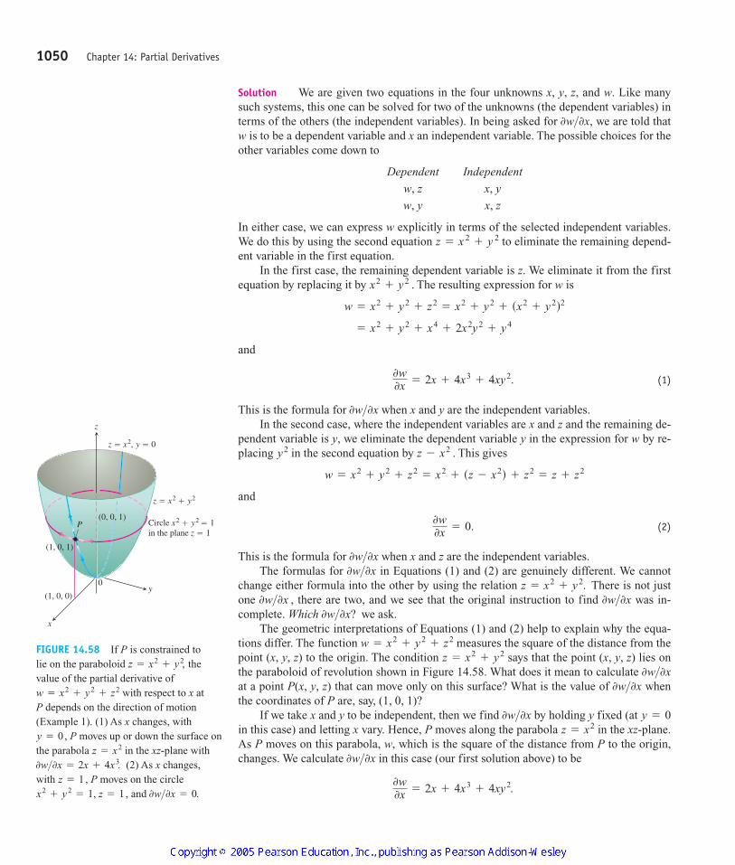
Solution We are given two equations in the four unknowns x, y, z, and w. Like manysuch systems, this one can be solved for two of the unknowns (the dependent variables) interms of the others (the independent variables). In being asked for we are told thatw is to be a dependent variable and x an independent variable. The possible choices for theother variables come down to
In either case, we can express w explicitly in terms of the selected independent variables.We do this by using the second equation to eliminate the remaining depend-ent variable in the first equation.
In the first case, the remaining dependent variable is z. We eliminate it from the firstequation by replacing it by The resulting expression for w is
and
(1)
This is the formula for when x and y are the independent variables.In the second case, where the independent variables are x and z and the remaining de-
pendent variable is y, we eliminate the dependent variable y in the expression for w by re-placing in the second equation by This gives
and
(2)
This is the formula for when x and z are the independent variables.The formulas for in Equations (1) and (2) are genuinely different. We cannot
change either formula into the other by using the relation There is not justone there are two, and we see that the original instruction to find was in-complete. Which we ask.
The geometric interpretations of Equations (1) and (2) help to explain why the equa-tions differ. The function measures the square of the distance from thepoint (x, y, z) to the origin. The condition says that the point (x, y, z) lies onthe paraboloid of revolution shown in Figure 14.58. What does it mean to calculate at a point P(x, y, z) that can move only on this surface? What is the value of whenthe coordinates of P are, say, (1, 0, 1)?
If we take x and y to be independent, then we find by holding y fixed (at in this case) and letting x vary. Hence, P moves along the parabola in the xz-plane.As P moves on this parabola, w, which is the square of the distance from P to the origin,changes. We calculate in this case (our first solution above) to be
0w0x = 2x + 4x3
+ 4xy2.
0w>0x
z = x2y = 00w>0x
0w>0x0w>0x
z = x2+ y2
w = x2+ y2
+ z2
0w>0x?0w>0x0w>0x ,
z = x2+ y2.
0w>0x0w>0x
0w0x = 0.
w = x2+ y2
+ z2= x2
+ sz - x2d + z2= z + z2
z - x2 .y2
0w>0x
0w0x = 2x + 4x3
+ 4xy2.
= x2+ y2
+ x4+ 2x2y2
+ y4
w = x2+ y2
+ z2= x2
+ y2+ sx2
+ y2d2
x2+ y2 .
z = x 2+ y 2
Dependent Independent
w, z x, y
w, y x, z
0w>0x,
1050 Chapter 14: Partial Derivatives
y
z
x
0
(1, 0, 0)
P(0, 0, 1)
z � x2, y � 0
z � x2 � y2
Circle x2 � y2 � 1in the plane z � 1
(1, 0, 1)
FIGURE 14.58 If P is constrained to lie on the paraboloid thevalue of the partial derivative of
with respect to x at P depends on the direction of motion(Example 1). (1) As x changes, with
P moves up or down the surface onthe parabola in the xz-plane with
(2) As x changes, with P moves on the circle
and 0w>0x = 0.x2+ y2
= 1, z = 1,z = 1,
0w>0x = 2x + 4x3.z = x2
y = 0,
w = x2+ y2
+ z2
z = x2+ y2,
4100 AWL/Thomas_ch14p965-1066 8/25/04 2:53 PM Page 1050
At the point P(1, 0, 1), the value of this derivative is
If we take x and z to be independent, then we find by holding z fixed while xvaries. Since the z-coordinate of P is 1, varying x moves P along a circle in the plane
As P moves along this circle, its distance from the origin remains constant, and w,being the square of this distance, does not change. That is,
as we found in our second solution.
How to Find When the Variables in AreConstrained by Another Equation
As we saw in Example 1, a typical routine for finding when the variables in thefunction are related by another equation has three steps. These steps applyto finding and as well.0w>0z0w>0y
w = ƒsx, y, zd0w>0x
w = ƒsx, y, zd�w>�x
0w0x = 0,
z = 1.
0w>0x
0w0x = 2 + 4 + 0 = 6.
14.9 Partial Derivatives with Constrained Variables 1051
1. Decide which variables are to be dependent and which are to be indepen-dent. (In practice, the decision is based on the physical or theoretical contextof our work. In the exercises at the end of this section, we say which vari-ables are which.)
2. Eliminate the other dependent variable(s) in the expression for w.
3. Differentiate as usual.
If we cannot carry out Step 2 after deciding which variables are dependent, we differ-entiate the equations as they are and try to solve for afterward. The next exampleshows how this is done.
EXAMPLE 2 Finding a Partial Derivative with Identified ConstrainedIndependent Variables
Find at the point if
and x and y are the independent variables.
Solution It is not convenient to eliminate z in the expression for w. We therefore differ-entiate both equations implicitly with respect to x, treating x and y as independent vari-ables and w and z as dependent variables. This gives
(3)0w0x = 2x + 2z
0z0x
w = x2+ y2
+ z2, z3- xy + yz + y3
= 1,
sx, y, zd = s2, -1, 1d0w>0x
0w>0x
4100 AWL/Thomas_ch14p965-1066 8/25/04 2:53 PM Page 1051
and
(4)
These equations may now be combined to express in terms of x, y, and z. We solveEquation (4) for to get
and substitute into Equation (3) to get
The value of this derivative at is
Notation
To show what variables are assumed to be independent in calculating a derivative, we canuse the following notation:
EXAMPLE 3 Finding a Partial Derivative with Constrained VariablesNotationally Identified
Find
Solution With x, y, z independent, we have
Arrow Diagrams
In solving problems like the one in Example 3, it often helps to start with an arrow dia-gram that shows how the variables and functions are related. If
w = x2+ y - z + sin t and x + y = t
= 2x + cos sx + yd.
a0w0x b y, z
= 2x + 0 - 0 + cos sx + yd 0
0x sx + yd
t = x + y, w = x2+ y - z + sin sx + yd
s0w>0xdy, z if w = x2+ y - z + sin t and x + y = t.
a0ƒ0y b x, t 0ƒ>0y with y, x and t independent
a0w0x b y 0w>0x with x and y independent
a0w0x b s2,-1,1d
= 2s2d +
2s -1ds1d-1 + 3s1d2 = 4 +
-22
= 3.
sx, y, zd = s2, -1, 1d
0w0x = 2x +
2yz
y + 3z2 .
0z0x =
y
y + 3z2
0z>0x0w>0x
3z2 0z0x - y + y
0z0x + 0 = 0.
1052 Chapter 14: Partial Derivatives
HISTORICAL BIOGRAPHY
Sonya Kovalevsky(1850–1891)
4100 AWL/Thomas_ch14p965-1066 8/25/04 2:54 PM Page 1052
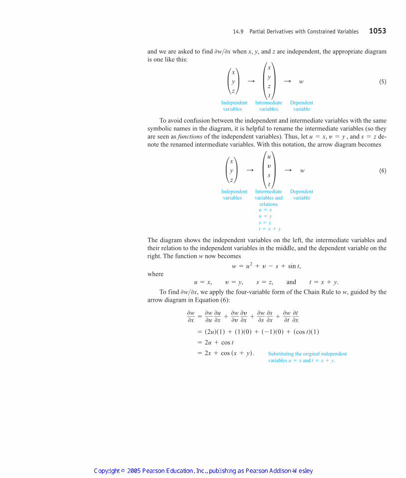
and we are asked to find when x, y, and z are independent, the appropriate diagramis one like this:
(5)
To avoid confusion between the independent and intermediate variables with the samesymbolic names in the diagram, it is helpful to rename the intermediate variables (so theyare seen as functions of the independent variables). Thus, let and de-note the renamed intermediate variables. With this notation, the arrow diagram becomes
(6)
The diagram shows the independent variables on the left, the intermediate variables andtheir relation to the independent variables in the middle, and the dependent variable on theright. The function w now becomes
where
To find we apply the four-variable form of the Chain Rule to w, guided by thearrow diagram in Equation (6):
= 2x + cos sx + yd .
= 2u + cos t
= s2uds1d + s1ds0d + s -1ds0d + scos tds1d
0w0x =
0w0u
0u0x +
0w0y
0y0x +
0w0s
0s0x +
0w0t
0t0x
0w>0x,
u = x, y = y, s = z, and t = x + y.
w = u2+ y - s + sin t,
£x
y
z
≥ : §u
y
s
t
¥ : w
s = zu = x, y = y ,
£x
y
z
≥ : §x
y
z
t
¥ : w
0w>0x
14.9 Partial Derivatives with Constrained Variables 1053
Independent Intermediate Dependentvariables variables and variable
relations
Independent Intermediate Dependentvariables variables variable
t = x + ys = zy = yu = x
Substituting the original independentvariables and t = x + y.u = x
4100 AWL/Thomas_ch14p965-1066 8/25/04 2:54 PM Page 1053
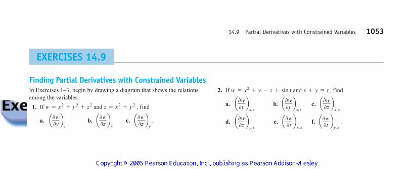
14.9 Partial Derivatives with Constrained Variables 1053
EXERCISES 14.9
Finding Partial Derivatives with Constrained VariablesIn Exercises 1–3, begin by drawing a diagram that shows the relationsamong the variables.
1. If and find
a. b. c. a0w0z b y
.a0w0z b x
a0w0y b z
z = x2+ y2 ,w = x2
+ y2+ z2
2. If and find
a. b. c.
d. e. f. a0w0t b y, z
.a0w0t b x, z
a0w0z b y, t
a0w0z b x, y
a0w0y b z, t
a0w0y b x, z
x + y = t ,w = x2+ y - z + sin t
4100 AWL/Thomas_ch14p965-1066 8/25/04 2:54 PM Page 1053
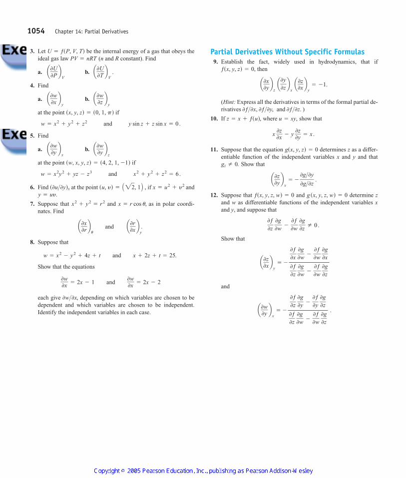
3. Let be the internal energy of a gas that obeys theideal gas law (n and R constant). Find
a. b.
4. Find
a. b.
at the point if
5. Find
a. b.
at the point if
6. Find at the point if and
7. Suppose that and as in polar coordi-nates. Find
8. Suppose that
Show that the equations
each give depending on which variables are chosen to bedependent and which variables are chosen to be independent.Identify the independent variables in each case.
0w>0x,
0w0x = 2x - 1 and 0w
0x = 2x - 2
w = x2- y2
+ 4z + t and x + 2z + t = 25.
a0x0r bu and a0r
0x b y.
x = r cos u,x2+ y2
= r2
y = uy.x = u2
+ y2su, yd = A22, 1 B ,s0u>0ydx
w = x2y2+ yz - z3 and x2
+ y2+ z2
= 6.
sw, x, y, zd = s4, 2, 1, -1d
a0w0y b z
a0w0y b x
w = x2+ y2
+ z2 and y sin z + z sin x = 0.
sx, y, zd = s0, 1, pd
a0w0z b y
a0w0x b y
a0U0Tb
V.a0U
0Pb
V
PV = nRTU = ƒsP, V, Td Partial Derivatives Without Specific Formulas
9. Establish the fact, widely used in hydrodynamics, that ifthen
(Hint: Express all the derivatives in terms of the formal partial de-rivatives and )
10. If where show that
11. Suppose that the equation determines z as a differ-entiable function of the independent variables x and y and that
Show that
12. Suppose that and determine zand w as differentiable functions of the independent variables xand y, and suppose that
Show that
and
a0w0y b x
= -
0ƒ0z
0g0y -
0ƒ0y
0g0z
0ƒ0z
0g0w -
0ƒ0w
0g0z
.
a0z0x b y
= -
0ƒ0x
0g0w -
0ƒ0w
0g0x
0ƒ0z
0g0w -
0ƒ0w
0g0z
0ƒ0z
0g0w -
0ƒ0w
0g0z Z 0.
g sx, y, z, wd = 0ƒsx, y, z, wd = 0
a0z0y b x
= -
0g>0y
0g>0z .
gz Z 0.
gsx, y, zd = 0
x 0z0x - y
0z0y = x .
u = xy,z = x + ƒsud,0ƒ>0z.0ƒ>0x, 0ƒ>0y,
a0x0y b z
a0y0z b x
a0z0x b y
= -1.
ƒsx, y, zd = 0,
1054 Chapter 14: Partial Derivatives
4100 AWL/Thomas_ch14p965-1066 8/25/04 2:54 PM Page 1054
1054 Chapter 14: Partial Derivatives
Taylor’s Formula for Two Variables
This section uses Taylor’s formula to derive the Second Derivative Test for local extremevalues (Section 14.7) and the error formula for linearizations of functions of two inde-pendent variables (Section 14.6). The use of Taylor’s formula in these derivations leads toan extension of the formula that provides polynomial approximations of all orders forfunctions of two independent variables.
Derivation of the Second Derivative Test
Let ƒ(x, y) have continuous partial derivatives in an open region R containing a point P(a, b)where (Figure 14.59). Let h and k be increments small enough to put theƒx = ƒy = 0
14.10
4100 AWL/Thomas_ch14p965-1066 8/25/04 2:54 PM Page 1054
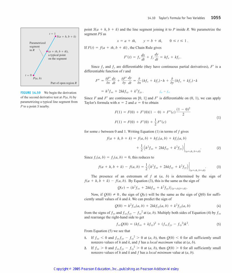
point and the line segment joining it to P inside R. We parametrize thesegment PS as
If the Chain Rule gives
Since and are differentiable (they have continuous partial derivatives), is adifferentiable function of t and
Since F and are continuous on [0, 1] and is differentiable on (0, 1), we can applyTaylor’s formula with and to obtain
(1)
for some c between 0 and 1. Writing Equation (1) in terms of ƒ gives
(2)
Since this reduces to
(3)
The presence of an extremum of ƒ at (a, b) is determined by the sign ofBy Equation (3), this is the same as the sign of
Now, if the sign of Q(c) will be the same as the sign of Q(0) for suffi-ciently small values of h and k. We can predict the sign of
(4)
from the signs of and at (a, b). Multiply both sides of Equation (4) by and rearrange the right-hand side to get
(5)
From Equation (5) we see that
1. If and at (a, b), then for all sufficiently smallnonzero values of h and k, and ƒ has a local maximum value at (a, b).
2. If and at (a, b), then for all sufficiently smallnonzero values of h and k and ƒ has a local minimum value at (a, b).
Qs0d 7 0ƒxx ƒyy - ƒxy2
7 0ƒxx 7 0
Qs0d 6 0ƒxx ƒyy - ƒxy2
7 0ƒxx 6 0
ƒxx Qs0d = shƒxx + kƒxyd2+ sƒxx ƒyy - ƒxy
2dk2.
ƒxxƒxx ƒyy - ƒxy2ƒxx
Qs0d = h2ƒxxsa, bd + 2hkƒxysa, bd + k2ƒyysa, bd
Qs0d Z 0 ,
Qscd = sh2ƒxx + 2hkƒxy + k2ƒyyd ƒ sa + ch,b + ckd .
ƒsa + h, b + kd - ƒsa, bd.
ƒsa + h, b + kd - ƒsa, bd =12
Ah2ƒxx + 2hkƒxy + k2ƒyy B `sa + ch, b + ckd
.
ƒxsa, bd = ƒysa, bd = 0,
+12
Ah2ƒxx + 2hkƒxy + k2ƒyy B `sa + ch, b + ckd
.
ƒsa + h, b + kd = ƒsa, bd + hƒxsa, bd + kƒysa, bd
Fs1d = Fs0d + F¿s0d +12
F–scd
Fs1d = Fs0d + F¿s0ds1 - 0d + F–scd s1 - 0d2
2
a = 0n = 2F¿F¿
fxy = fyx = h2ƒxx + 2hkƒxy + k2ƒyy .
F– =0F¿
0x dxdt
+0F¿
0y dydt
=0
0x shƒx + kƒyd # h +0
0y shƒx + kƒyd # k
F¿ƒyƒx
F¿std = ƒx dxdt
+ ƒy dydt
= hƒx + kƒy .
Fstd = ƒsa + th, b + tkd ,
x = a + th, y = b + tk, 0 … t … 1 .
Ssa + h, b + kd
14.10 Taylor’s Formula for Two Variables 1055
Part of open region R
(a � th, b � tk),a typical pointon the segment
P(a, b)t � 0
Parametrizedsegmentin R
t � 1S(a � h, b � k)
FIGURE 14.59 We begin the derivationof the second derivative test at P(a, b) byparametrizing a typical line segment fromP to a point S nearby.
4100 AWL/Thomas_ch14p965-1066 8/25/04 2:54 PM Page 1055
3. If at (a, b), there are combinations of arbitrarily small nonzero val-ues of h and k for which and other values for which Arbitrarilyclose to the point on the surface there are points above
and points below so ƒ has a saddle point at (a, b).
4. If another test is needed. The possibility that Q(0) equals zero pre-vents us from drawing conclusions about the sign of Q(c).
The Error Formula for Linear Approximations
We want to show that the difference E(x, y), between the values of a function ƒ(x, y), andits linearization L(x, y) at satisfies the inequality
The function ƒ is assumed to have continuous second partial derivatives throughout anopen set containing a closed rectangular region R centered at The number M is anupper bound for and on R.
The inequality we want comes from Equation (2). We substitute and for a and b,and and for h and k, respectively, and rearrange the result as
This equation reveals that
Hence, if M is an upper bound for the values of and on R,
Taylor’s Formula for Functions of Two Variables
The formulas derived earlier for and can be obtained by applying to ƒ(x, y) the oper-ators
These are the first two instances of a more general formula,
(6)F sndstd =
dn
dtn Fstd = ah 0
0x + k 0
0y bn
ƒsx, yd ,
ah 0
0x + k 0
0y b and ah 0
0x + k 0
0y b2
= h2 0
2
0x2 + 2hk 0
2
0x 0y + k2 0
2
0y2 .
F–F¿
=12
Ms ƒ x - x0 ƒ + ƒ y - y0 ƒ d2.
ƒ E ƒ …12
A ƒ x - x0 ƒ2 M + 2 ƒ x - x0 ƒ ƒ y - y0 ƒ M + ƒ y - y0 ƒ
2M Bƒ ƒyy ƒƒ ƒxx ƒ , ƒ ƒxy ƒ ,
ƒ E ƒ …12
A ƒ x - x0 ƒ2
ƒ ƒxx ƒ + 2 ƒ x - x0 ƒ ƒ y - y0 ƒ ƒ ƒxy ƒ + ƒ y - y0 ƒ2
ƒ ƒyy ƒ B .
+12
A sx - x0d2ƒxx + 2sx - x0ds y - y0dƒxy + s y - y0d2ƒyy B ` sx0 +csx-x0d, y0 +cs y-y0dd. ('''''''''''''''')'''''''''''''''''*
error Esx, yd
ƒsx, yd = ƒsx0 , y0d + ƒxsx0 , y0dsx - x0d + ƒysx0 , y0ds y - y0d('''''''')'''''''''''''*
linearization Lsx, yd
y - y0x - x0
y0x0
ƒ ƒxy ƒƒ ƒxx ƒ , ƒ ƒyy ƒ ,sx0 , y0d.
ƒ Esx, yd ƒ …12
Ms ƒ x - x0 ƒ + ƒ y - y0 ƒ d2.
sx0 , y0d
ƒxx ƒyy - ƒxy2
= 0,
P0 ,P0
z = ƒsx, ydP0sa, b, ƒsa, bddQs0d 6 0.Qs0d 7 0,
ƒxx ƒyy - ƒxy2
6 0
1056 Chapter 14: Partial Derivatives
4100 AWL/Thomas_ch14p965-1066 8/25/04 2:54 PM Page 1056
which says that applying gives the same result as applying the operator
to ƒ(x, y) after expanding it by the Binomial Theorem.If partial derivatives of ƒ through order are continuous throughout a rectangu-
lar region centered at (a, b), we may extend the Taylor formula for F(t) to
and take to obtain
When we replace the first n derivatives on the right of this last series by their equivalentexpressions from Equation (6) evaluated at and add the appropriate remainder term,we arrive at the following formula.
t = 0
Fs1d = Fs0d + F¿s0d +
F–s0d2!
+Á
+
F snds0dn!
+ remainder.
t = 1
Fstd = Fs0d + F¿s0dt +
F–s0d2!
t2+
Á+
F snds0dn!
t snd+ remainder,
n + 1
ah 0
0x + k 0
0y bn
dn>dtn to Fstd
14.10 Taylor’s Formula for Two Variables 1057
Taylor’s Formula for ƒ(x, y) at the Point (a, b)Suppose ƒ(x, y) and its partial derivatives through order are continuous throughout an open rectangular region R cen-tered at a point (a, b). Then, throughout R,
(7)+1
sn + 1d! ah
0
0x + k 0
0y bn + 1
ƒ `sa + ch,b + ckd
.
+13!
sh3ƒxxx + 3h2kƒxxy + 3hk2ƒxyy + k3ƒyyyd ƒ sa,bd +Á
+1n!
ah 0
0x + k 0
0y bn
ƒ `sa,bd
ƒsa + h, b + kd = ƒsa, bd + shƒx + kƒyd ƒ sa,bd +12!
sh2ƒxx + 2hkƒxy + k2ƒyyd ƒ sa,bd
n + 1
Taylor’s Formula for ƒ(x, y) at the Origin
(8)+1
sn + 1d! ax
0
0x + y 0
0y bn + 1
ƒ `scx,cyd
+13!
sx3ƒxxx + 3x2yƒxxy + 3xy2ƒxyy + y3ƒyyyd +Á
+1n!
ax 0
0x + y 0
0y bn
ƒ
ƒsx, yd = ƒs0, 0d + xƒx + yƒy +12!
sx2ƒxx + 2xyƒxy + y2ƒyyd
The first n derivative terms are evaluated at (a, b). The last term is evaluated at some pointon the line segment joining (a, b) and
If and we treat h and k as independent variables (denoting them nowby x and y), then Equation (7) assumes the following simpler form.
sa, bd = s0, 0dsa + h, b + kd.sa + ch, b + ckd
4100 AWL/Thomas_ch14p965-1066 8/25/04 2:54 PM Page 1057
The first n derivative terms are evaluated at (0, 0). The last term is evaluated at a point onthe line segment joining the origin and (x, y).
Taylor’s formula provides polynomial approximations of two-variable functions. Thefirst n derivative terms give the polynomial; the last term gives the approximation error.The first three terms of Taylor’s formula give the function’s linearization. To improve onthe linearization, we add higher power terms.
EXAMPLE 1 Finding a Quadratic Approximation
Find a quadratic approximation to near the origin. How accurate is theapproximation if and
Solution We take in Equation (8):
with
we have
The error in the approximation is
The third derivatives never exceed 1 in absolute value because they are products of sinesand cosines. Also, and Hence
(rounded up). The error will not exceed 0.00134 if and ƒ y ƒ … 0.1.ƒ x ƒ … 0.1
ƒ Esx, yd ƒ …16
ss0.1d3+ 3s0.1d3
+ 3s0.1d3+ s0.1d3d =
86
s0.1d3… 0.00134
ƒ y ƒ … 0.1.ƒ x ƒ … 0.1
Esx, yd =16
sx3ƒxxx + 3x2yƒxxy + 3xy2ƒxyy + y3ƒyyyd ƒ scx,cyd .
sin x sin y L xy.
sin x sin y L 0 + 0 + 0 +12
sx2s0d + 2xys1d + y2s0dd,
ƒys0, 0d = sin x cos y ƒ s0,0d = 0, ƒyys0, 0d = -sin x sin y ƒ s0,0d = 0,
ƒxs0, 0d = cos x sin y ƒ s0,0d = 0, ƒxys0, 0d = cos x cos y ƒ s0,0d = 1,
ƒs0, 0d = sin x sin y ƒ s0,0d = 0, ƒxxs0, 0d = -sin x sin y ƒ s0,0d = 0,
+16
sx3ƒxxx + 3x2yƒxxy + 3xy2ƒxyy + y3ƒyyydscx,cyd
ƒsx, yd = ƒs0, 0d + sxƒx + yƒyd +12
sx2ƒxx + 2xyƒxy + y2ƒyyd
n = 2
ƒ y ƒ … 0.1? ƒ x ƒ … 0.1ƒsx, yd = sin x sin y
1058 Chapter 14: Partial Derivatives
4100 AWL/Thomas_ch14p965-1066 8/25/04 2:54 PM Page 1058
1058 Chapter 14: Partial Derivatives
EXERCISES 14.10
Finding Quadratic and Cubic ApproximationsIn Exercises 1–10, use Taylor’s formula for ƒ(x, y) at the origin to findquadratic and cubic approximations of ƒ near the origin.
1. 2. ƒsx, yd = ex cos yƒsx, yd = xey
3. 4.
5. 6.
7. 8. ƒsx, yd = cos sx2+ y2dƒsx, yd = sin sx2
+ y2dƒsx, yd = ln s2x + y + 1dƒsx, yd = ex ln s1 + ydƒsx, yd = sin x cos yƒsx, yd = y sin x
4100 AWL/Thomas_ch14p965-1066 8/25/04 2:54 PM Page 1058
9. 10.
11. Use Taylor’s formula to find a quadratic approximation ofat the origin. Estimate the error in the ap-
proximation if and ƒ y ƒ … 0.1.ƒ x ƒ … 0.1ƒsx, yd = cos x cos y
ƒsx, yd =
11 - x - y + xy
ƒsx, yd =
11 - x - y
12. Use Taylor’s formula to find a quadratic approximation of at the origin. Estimate the error in the approximation if and ƒ y ƒ … 0.1.
ƒ x ƒ … 0.1ex sin y
1059
4100 AWL/Thomas_ch14p965-1066 8/25/04 2:54 PM Page 1059
14.10 Taylor’s Formula for Two Variables
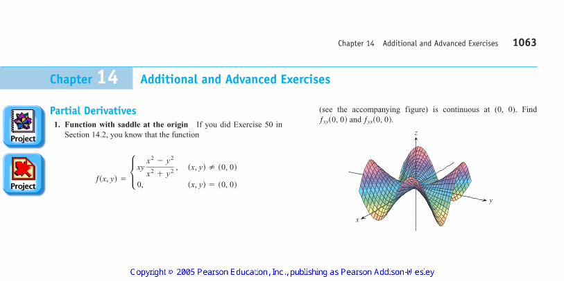
Chapter 14 Additional and Advanced Exercises 1063
Chapter 14 Additional and Advanced Exercises
Partial Derivatives1. Function with saddle at the origin If you did Exercise 50 in
Section 14.2, you know that the function
ƒsx, yd = L xy x2
- y2
x2+ y2 , sx, yd Z s0, 0d
0, sx, yd = s0, 0d
(see the accompanying figure) is continuous at (0, 0). Findand
z
y
x
ƒyxs0, 0d.ƒxys0, 0d
4100 AWL/Thomas_ch14p965-1066 8/25/04 2:54 PM Page 1063
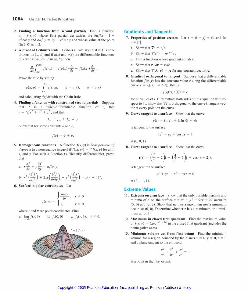
2. Finding a function from second partials Find a functionwhose first partial derivatives are
and and whose value at the point(ln 2, 0) is ln 2.
3. A proof of Leibniz’s Rule Leibniz’s Rule says that if ƒ is con-tinuous on [a, b] and if u(x) and y(x) are differentiable functionsof x whose values lie in [a, b], then
Prove the rule by setting
and calculating dg dx with the Chain Rule.
4. Finding a function with constrained second partials Supposethat ƒ is a twice-differentiable function of r, that
and that
Show that for some constants a and b,
5. Homogeneous functions A function ƒ(x, y) is homogeneous ofdegree n (n a nonnegative integer) if for all t,x, and y. For such a function (sufficiently differentiable), provethat
a.
b.
6. Surface in polar coordinates Let
where r and are polar coordinates. Find
a. b. c.
z � f (r, �)
ƒusr, ud, r Z 0.ƒrs0, 0dlimr:0
ƒsr, udu
ƒsr, ud = L sin 6r6r
, r Z 0
1, r = 0,
x2 a02ƒ
0x2 b + 2xy a 02ƒ
0x0y b + y2 a02ƒ
0y2 b = nsn - 1dƒ.
x 0ƒ0x + y
0ƒ0y = nƒsx, yd
ƒstx, tyd = t nƒsx, yd
ƒsrd =
ar + b.
ƒxx + ƒyy + ƒzz = 0.
r = 2x2+ y2
+ z2 ,
>gsu, yd = L
y
u ƒstd dt, u = usxd, y = ysxd
ddxL
ysxd
usxd ƒstd dt = ƒsysxdd
dydx
- ƒsusxdd dudx
.
0w>0y = 2y - ex sin yex cos y0w>0x = 1 +w = ƒsx, yd
Gradients and Tangents7. Properties of position vectors Let and let
a. Show that
b. Show that
c. Find a function whose gradient equals r.
d. Show that
e. Show that for any constant vector A.
8. Gradient orthogonal to tangent Suppose that a differentiablefunction ƒ(x, y) has the constant value c along the differentiablecurve that is
for all values of t. Differentiate both sides of this equation with re-spect to t to show that is orthogonal to the curve’s tangent vec-tor at every point on the curve.
9. Curve tangent to a surface Show that the curve
is tangent to the surface
at (0, 0, 1).
10. Curve tangent to a surface Show that the curve
is tangent to the surface
at
Extreme Values11. Extrema on a surface Show that the only possible maxima and
minima of z on the surface occur at(0, 0) and (3, 3). Show that neither a maximum nor a minimumoccurs at (0, 0). Determine whether z has a maximum or a mini-mum at (3, 3).
12. Maximum in closed first quadrant Find the maximum valueof in the closed first quadrant (includes thenonnegative axes).
13. Minimum volume cut from first octant Find the minimumvolume for a region bounded by the planes and a plane tangent to the ellipsoid
at a point in the first octant.
x2
a2 +
y2
b2 +
z2
c2 = 1
x = 0, y = 0, z = 0
ƒsx, yd = 6xye-s2x + 3yd
z = x3+ y3
- 9xy + 27
s0, -1, 1d.
x3+ y3
+ z3- xyz = 0
rstd = at3
4- 2b i + a4t - 3bj + cos st - 2dk
xz2- yz + cos xy = 1
rstd = sln tdi + st ln tdj + tk
§ƒ
ƒsgstd, hstdd = c
x = gstd, y = hstd;
§sA # rd = A
r # dr = r dr.
§srnd = nrn - 2r.
§r = r>r.
r = ƒ r ƒ .r = xi + yj + zk
1064 Chapter 14: Partial Derivatives
4100 AWL/Thomas_ch14p965-1066 8/25/04 2:54 PM Page 1064
14. Minimum distance from line to parabola in xy-plane Byminimizing the function subject to the constraints and find the mini-mum distance in the xy-plane from the line to theparabola
Theory and Examples15. Boundedness of first partials implies continuity Prove the
following theorem: If ƒ(x, y) is defined in an open region R of thexy-plane and if and are bounded on R, then ƒ(x, y) is contin-uous on R. (The assumption of boundedness is essential.)
16. Suppose that is a smooth curve inthe domain of a differentiable function ƒ(x, y, z). Describe the re-lation between dƒ dt, and What can be said about
and v at interior points of the curve where ƒ has extreme val-ues relative to its other values on the curve? Give reasons for youranswer.
17. Finding functions from partial derivatives Suppose that ƒand g are functions of x and y such that
and suppose that
Find ƒ(x, y) and g(x, y).
18. Rate of change of the rate of change We know that if ƒ(x, y) isa function of two variables and if is a unit vector, then
is the rate of change of ƒ(x, y)at (x, y) in the direction of u. Give a similar formula for the rate ofchange of the rate of change of ƒ(x, y) at (x, y) in the direction u.
19. Path of a heat-seeking particle A heat-seeking particle has theproperty that at any point (x, y) in the plane it moves in the direc-tion of maximum temperature increase. If the temperature at (x, y)is find an equation for the pathof a heat-seeking particle at the point
20. Velocity after a ricochet A particle traveling in a straight linewith constant velocity passes through the point (0, 0, 30) and hits the surface The particle rico-chets off the surface, the angle of reflection being equal to theangle of incidence. Assuming no loss of speed, what is the veloc-ity of the particle after the ricochet? Simplify your answer.
21. Directional derivatives tangent to a surface Let S be the sur-face that is the graph of Suppose thatthe temperature in space at each point (x, y, z) is
a. Among all the possible directions tangential to the surface Sat the point (0, 0, 10), which direction will make the rate ofchange of temperature at (0, 0, 10) a maximum?
y2z + 4x + 14y + z.Tsx, y, zd = x2y +
ƒsx, yd = 10 - x2- y2 .
z = 2x2+ 3y2 .
i + j - 5k
sp>4, 0d.y = ƒsxdTsx, yd = -e-2y cos x,
Du ƒsx, yd = ƒxsx, yda + ƒysx, ydbu = ai + bj
0ƒ0x = 0, ƒs1, 2d = gs1, 2d = 5 and ƒs0, 0d = 4.
0ƒ0y =
0g0x and 0ƒ
0x =
0g0y ,
§ƒv = dr>dt.§ƒ ,>
rstd = gstdi + hstdj + kstdk
ƒyƒx
y2= x.
y = x + 1u = y2,y = x + 1
ƒsx, y, u, yd = sx - ud2+ sy - yd2
b. Which direction tangential to S at the point (1, 1, 8) will makethe rate of change of temperature a maximum?
22. Drilling another borehole On a flat surface of land, geologistsdrilled a borehole straight down and hit a mineral deposit at 1000ft. They drilled a second borehole 100 ft to the north of the firstand hit the mineral deposit at 950 ft. A third borehole 100 ft eastof the first borehole struck the mineral deposit at 1025 ft. The ge-ologists have reasons to believe that the mineral deposit is in theshape of a dome, and for the sake of economy, they would like tofind where the deposit is closest to the surface. Assuming the sur-face to be the xy-plane, in what direction from the first boreholewould you suggest the geologists drill their fourth borehole?
The One-Dimensional Heat EquationIf w(x, t) represents the temperature at position x at time t in a uniformconducting rod with perfectly insulated sides (see the accompanyingfigure), then the partial derivatives and satisfy a differentialequation of the form
This equation is called the one-dimensional heat equation. The valueof the positive constant is determined by the material from whichthe rod is made. It has been determined experimentally for a broadrange of materials. For a given application, one finds the appropriatevalue in a table. For dry soil, for example,
In chemistry and biochemistry, the heat equation is known as thediffusion equation. In this context, w(x, t) represents the concentra-tion of a dissolved substance, a salt for instance, diffusing along a tubefilled with liquid. The value of w(x, t) is the concentration at point x attime t. In other applications, w(x, t) represents the diffusion of a gasdown a long, thin pipe.
In electrical engineering, the heat equation appears in the forms
and
ixx = RCit .
yxx = RCyt
x
x
x � 0
w(x, t) is the temperaturehere at time t.
c2= 0.19 ft2>day.
c2
wxx =
1c2 wt .
wtwxx
Chapter 14 Additional and Advanced Exercises 1065
4100 AWL/Thomas_ch14p965-1066 8/25/04 2:54 PM Page 1065
These equations describe the voltage y and the flow of current i in acoaxial cable or in any other cable in which leakage and inductanceare negligible. The functions and constants in these equations are
isx, td = current at point x at time t.
C = capacitance to ground per unit of cable length
R = resistance per unit length
ysx, td = voltage at point x at time t
23. Find all solutions of the one-dimensional heat equation of theform where r is a constant.
24. Find all solutions of the one-dimensional heat equation that havethe form and satisfy the conditions that and What happens to these solutions as t : q?wsL, td = 0.
ws0, td = 0w = ert sin kx
w = ert sin px,
1066 Chapter 14: Partial Derivatives
4100 AWL/Thomas_ch14p965-1066 8/25/04 2:54 PM Page 1066
1060 Chapter 14: Partial Derivatives
Chapter 14 Practice Exercises
Domain, Range, and Level CurvesIn Exercises 1–4, find the domain and range of the given function andidentify its level curves. Sketch a typical level curve.
1. 2.
3. 4.
In Exercises 5–8, find the domain and range of the given function andidentify its level surfaces. Sketch a typical level surface.
5. 6.
7.
8.
Evaluating LimitsFind the limits in Exercises 9–14.
9. 10.
11. 12.
13. 14.
By considering different paths of approach, show that the limits in Ex-ercises 15 and 16 do not exist.
15. 16.
17. Continuous extension Let forIs it possible to define ƒ(0, 0) in a way that
makes ƒ continuous at the origin? Why?
18. Continuous extension Let
Is ƒ continuous at the origin? Why?
Partial DerivativesIn Exercises 19–24, find the partial derivative of the function withrespect to each variable.
19.
20.
21.
22. hsx, y, zd = sin s2px + y - 3zd
ƒsR1, R2, R3d =
1R1
+
1R2
+
1R3
ƒsx, yd =
12
ln sx2+ y2d + tan-1
yx
gsr, ud = r cos u + r sin u
ƒsx, yd = L sin sx - ydƒ x ƒ + ƒ y ƒ
, ƒ x ƒ + ƒ y ƒ Z 0
0, sx, yd = s0, 0d.
sx, yd Z s0, 0d .ƒsx, yd = sx2
- y2d>sx2+ y2d
limsx,yd : s0,0d
xy Z 0
x2
+ y2
xylimsx,yd : s0,0d
y Z x2
y
x2- y
limP: s1,-1,-1d
tan-1 sx + y + zdlimP: s1, -1, ed
ln ƒ x + y + z ƒ
limsx,yd: s1,1d
x3y3
- 1
xy - 1lim
sx,yd: s1,1d
x - y
x2- y2
limsx,yd: s0,0d
2 + y
x + cos ylimsx,yd: sp, ln 2d
ey cos x
ksx, y, zd =
1x2
+ y2+ z2
+ 1
hsx, y, zd =
1x2
+ y2+ z2
gsx, y, zd = x2+ 4y2
+ 9z2ƒsx, y, zd = x2+ y2
- z
gsx, yd = 2x2- ygsx, yd = 1>xy
ƒsx, yd = ex + yƒsx, yd = 9x2+ y2
23. (the ideal gas law)
24.
Second-Order PartialsFind the second-order partial derivatives of the functions in Exercises25–28.
25. 26.
27.
28.
Chain Rule Calculations29. Find dw dt at if and
30. Find dw dt at if and
31. Find and when and if
32. Find and when if
and
33. Find the value of the derivative of withrespect to t on the curve at
34. Show that if is any differentiable function of s and ifthen
Implicit DifferentiationAssuming that the equations in Exercises 35 and 36 define y as a dif-ferentiable function of x, find the value of dy dx at point P.
35.
36.
Directional DerivativesIn Exercises 37–40, find the directions in which ƒ increases and de-creases most rapidly at and find the derivative of ƒ in each direc-tion. Also, find the derivative of ƒ at in the direction of the vector v.
37.
38.
39.
v = 2i + 3j + 6k
ƒsx, y, zd = ln s2x + 3y + 6zd, P0s -1, -1, 1d,ƒsx, yd = x2e-2y, P0s1, 0d, v = i + j
ƒsx, yd = cos x cos y, P0sp>4, p>4d, v = 3i + 4j
P0
P0
2xy + ex + y- 2 = 0, Ps0, ln 2d
1 - x - y2- sin xy = 0, Ps0, 1d
>
0w0x - 5
0w0y = 0.
s = y + 5x ,w = ƒssd
t = 1 .x = cos t, y = sin t, z = cos 2tƒsx, y, zd = xy + yz + xz
x = 2eu cos y.ln21 + x2- tan-1 x
w =u = y = 00w>0y0w>0u
x = r + sin s, y = rs.w = sin s2x - yd, s = 0r = p0w>0s0w>0r
z = pt.y = t - 1 + ln t ,w = xey
+ y sin z - cos z, x = 22t, t = 1>ln st + 1d.
y =w = sin sxy + pd, x = et ,t = 0>
ƒsx, yd = y2- 3xy + cos y + 7ey
ƒsx, yd = x + xy - 5x3+ ln sx2
+ 1d
gsx, yd = ex+ y sin xgsx, yd = y +
xy
ƒsr, l, T, wd =
12rl
A Tpw
Psn, R, T, Vd =
nRTV
4100 AWL/Thomas_ch14p965-1066 8/25/04 2:54 PM Page 1060
40.
41. Derivative in velocity direction Find the derivative ofin the direction of the velocity vector of the helix
at
42. Maximum directional derivative What is the largest value thatthe directional derivative of can have at the point(1, 1, 1)?
43. Directional derivatives with given values At the point (1, 2),the function ƒ(x, y) has a derivative of 2 in the direction toward (2, 2) and a derivative of in the direction toward (1, 1).a. Find and
b. Find the derivative of ƒ at (1, 2) in the direction toward thepoint (4, 6).
44. Which of the following statements are true if ƒ(x, y) is differen-tiable at Give reasons for your answers.
a. If u is a unit vector, the derivative of ƒ at in thedirection of u is
b. The derivative of ƒ at in the direction of u is a vector.
c. The directional derivative of ƒ at has its greatest valuein the direction of
d. At vector is normal to the curve
Gradients, Tangent Planes, and Normal LinesIn Exercises 45 and 46, sketch the surface together with
at the given points.
45.
46.
In Exercises 47 and 48, find an equation for the plane tangent to thelevel surface at the point Also, find parametricequations for the line that is normal to the surface at
47.
48.
In Exercises 49 and 50, find an equation for the plane tangent to thesurface at the given point.
49.
50.
In Exercises 51 and 52, find equations for the lines that are tangentand normal to the level curve at the point Then sketchthe lines and level curve together with at
51. 52.y2
2-
x2
2=
32
, P0s1, 2dy - sin x = 1, P0sp, 1d
P0 .§ƒP0 .ƒsx, yd = c
z = 1>sx2+ y2d, s1, 1, 1>2d
z = ln sx2+ y2d, s0, 1, 0d
z = ƒsx, yd
x2+ y2
+ z = 4, P0s1, 1, 2dx2
- y - 5z = 0, P0s2, -1, 1dP0 .
P0 .ƒsx, y, zd = c
y2+ z2
= 4; s2, ;2, 0d, s2, 0, ;2dx2
+ y + z2= 0; s0, -1, ;1d, s0, 0, 0d
§ƒƒsx, y, zd = c
ƒsx, yd = ƒsx0 , y0d.§ƒsx0 , y0d ,
§ƒ .sx0 , y0d
sx0 , y0dsƒxsx0 , y0di + ƒysx0 , y0djd # u.
sx0 , y0dsx0 , y0d ?
ƒys1, 2d .ƒxs1, 2d-2
ƒsx, y, zd = xyz
t = p>3.
rstd = scos 3tdi + ssin 3tdj + 3tk
ƒsx, y, zd = xyz
v = i + j + k
ƒsx, y, zd = x2+ 3xy - z2
+ 2y + z + 4, P0s0, 0, 0d, Tangent Lines to CurvesIn Exercises 53 and 54, find parametric equations for the line that istangent to the curve of intersection of the surfaces at the given point.
53. Surfaces:
Point: (1, 1, 1 2)
54. Surfaces:
Point: (1 2, 1, 1 2)
LinearizationsIn Exercises 55 and 56, find the linearization L(x, y) of the functionƒ(x, y) at the point Then find an upper bound for the magnitude ofthe error E in the approximation over the rectangle R.
55.
56.
Find the linearizations of the functions in Exercises 57 and 58 at thegiven points.
57. at (1, 0, 0) and (1, 1, 0)
58. at and
Estimates and Sensitivity to Change59. Measuring the volume of a pipeline You plan to calculate the
volume inside a stretch of pipeline that is about 36 in. in diameterand 1 mile long. With which measurement should you be morecareful, the length or the diameter? Why?
60. Sensitivity to change Near the point (1, 2), is more sensitive to changes in x or to changes
in y? How do you know?
61. Change in an electrical circuit Suppose that the current I (am-peres) in an electrical circuit is related to the voltage V (volts) andthe resistance R (ohms) by the equation If the voltagedrops from 24 to 23 volts and the resistance drops from 100 to80 ohms, will I increase or decrease? By about how much? Is thechange in I more sensitive to change in the voltage or to change inthe resistance? How do you know?
62. Maximum error in estimating the area of an ellipse Ifand to the nearest millimeter, what should
you expect the maximum percentage error to be in the calculatedarea of the ellipse
63. Error in estimating a product Let and where u and y are positive independent variables.
a. If u is measured with an error of 2% and y with an error of 3%,about what is the percentage error in the calculated value of y ?
z = u + y,y = uy
x2>a2+ y2>b2
= 1?A = pab
b = 16 cma = 10 cm
I = V>R .
x2- xy + y2
- 3ƒsx, yd =
p>4, 0dsp>4,s0, 0, p>4dƒsx, y, zd = 22 cos x sin s y + zdƒsx, y, zd = xy + 2yz - 3xz
R: ƒ x - 1 ƒ … 0.1, ƒ y - 1 ƒ … 0.2
ƒsx, yd = xy - 3y2+ 2, P0s1, 1d
R: ` x -
p
4` … 0.1, ` y -
p
4` … 0.1
ƒsx, yd = sin x cos y, P0sp>4, p>4dƒsx, yd L Lsx, yd
P0 .
>>x + y2
+ z = 2, y = 1
>x2
+ 2y + 2z = 4, y = 1
Chapter 14 Practice Exercises 1061
4100 AWL/Thomas_ch14p965-1066 8/25/04 2:54 PM Page 1061
b. Show that the percentage error in the calculated value of z isless than the percentage error in the value of y.
64. Cardiac index To make different people comparable in studiesof cardiac output (Section 3.7, Exercise 25), researchers dividethe measured cardiac output by the body surface area to find thecardiac index C:
The body surface area B of a person with weight w and height h isapproximated by the formula
which gives B in square centimeters when w is measured in kilo-grams and h in centimeters. You are about to calculate the cardiacindex of a person with the following measurements:
Which will have a greater effect on the calculation, a 1-kg error inmeasuring the weight or a 1-cm error in measuring the height?
Local ExtremaTest the functions in Exercises 65–70 for local maxima and minimaand saddle points. Find each function’s value at these points.
65.
66.
67.
68.
69.
70.
Absolute ExtremaIn Exercises 71–78, find the absolute maximum and minimum valuesof ƒ on the region R.
71.
R: The triangular region cut from the first quadrant by the line
72.
R: The rectangular region in the first quadrant bounded by the co-ordinate axes and the lines and
73.
R: The square region enclosed by the lines and
74.
R: The square region bounded by the coordinate axes and the linesin the first quadrantx = 2, y = 2
ƒsx, yd = 2x + 2y - x2- y2
y = ;2x = ;2
ƒsx, yd = y2- xy - 3y + 2x
y = 2x = 4
ƒsx, yd = x2- y2
- 2x + 4y + 1
x + y = 4
ƒsx, yd = x2+ xy + y2
- 3x + 3y
ƒsx, yd = x4- 8x2
+ 3y2- 6y
ƒsx, yd = x3+ y3
+ 3x2- 3y2
ƒsx, yd = x3+ y3
- 3xy + 15
ƒsx, yd = 2x3+ 3xy + 2y3
ƒsx, yd = 5x2+ 4xy - 2y2
+ 4x - 4y
ƒsx, yd = x2- xy + y2
+ 2x + 2y - 4
Cardiac output: 7 L>min
Weight: 70 kg
Height: 180 cm
B = 71.84w0.425h0.725 ,
C =
cardiac output
body surface area.
75.
R: The triangular region bounded below by the x-axis, above bythe line and on the right by the line
76.
R: The triangular region bounded below by the line above by the line and on the right by the line
77.
R: The square region enclosed by the lines and
78.
R: The square region enclosed by the lines and
Lagrange Multipliers79. Extrema on a circle Find the extreme values of
on the circle
80. Extrema on a circle Find the extreme values of onthe circle
81. Extrema in a disk Find the extreme values of on the unit disk
82. Extrema in a disk Find the extreme values of on the disk
83. Extrema on a sphere Find the extreme values of on the unit sphere
84. Minimum distance to origin Find the points on the surfaceclosest to the origin.
85. Minimizing cost of a box A closed rectangular box is to havevolume The cost of the material used in the box is
for top and bottom, for front and back,and for the remaining sides. What dimensions mini-mize the total cost of materials?
86. Least volume Find the plane that passesthrough the point (2, 1, 2) and cuts off the least volume from thefirst octant.
87. Extrema on curve of intersecting surfaces Find the extremevalues of on the curve of intersection of theright circular cylinder and the hyperbolic cylinder
88. Minimum distance to origin on curve of intersecting planeand cone Find the point closest to the origin on the curve of in-tersection of the plane and the cone
Partial Derivatives with Constrained VariablesIn Exercises 89 and 90, begin by drawing a diagram that shows therelations among the variables.
89. If and find
a. b. c. a0w0z b y
.a0w0z b x
a0w0y b z
z = x2- y2w = x2eyz
2x2+ 2y2.
z2=x + y + z = 1
xz = 1.x2
+ y2= 1
ƒsx, y, zd = xs y + zd
x>a + y>b + z>c = 1
c cents>cm2b cents>cm2a cents>cm2
V cm3.
z2- xy = 4
x2+ y2
+ z2= 1.x - y + z
ƒsx, y, zd =
x2+ y2
… 9.x2+ y2
- 3x - xyƒsx, yd =
x2+ y2
… 1.x2+ 3y2
+ 2yƒsx, yd =
x2+ y2
= 1.ƒsx, yd = xy
x2+ y2
= 1.x3+ y2
ƒsx, yd =
y = ;1x = ;1
ƒsx, yd = x3+ 3xy + y3
+ 1
y = ;1x = ;1
ƒsx, yd = x3+ y3
+ 3x2- 3y2
x = 2y = x,y = -2,
ƒsx, yd = 4xy - x4- y4
+ 16
x = 2y = x + 2,
ƒsx, yd = x2- y2
- 2x + 4y
1062 Chapter 14: Partial Derivatives
4100 AWL/Thomas_ch14p965-1066 8/25/04 2:54 PM Page 1062
90. Let be the internal energy of a gas that obeys theideal gas law (n and R constant). Find
a. b.
Theory and Examples91. Let and Find
and and express your answers in terms of r and
92. Let and Express and in terms of and the constants a and b.
93. If a and b are constants, and show that
94. Using the Chain Rule If and find and by the Chain Rule. Then
check your answer another way.
95. Angle between vectors The equations anddefine u and as differentiable functions of x
and y. Show that the angle between the vectors
is constant.
96. Polar coordinates and second derivatives Introducing polarcoordinates and changes ƒ(x, y) to Find the value of at the point given that
at that point.
0ƒ0x =
0ƒ0y =
02ƒ
0x2 =
02ƒ
0y2 = 1
sr, ud = s2, p>2d,02g>0u2
gsr, ud.y = r sin ux = r cos u
0u0x i +
0u0y j and 0y
0x i +
0y0y j
yeu sin y - y = 0eu cos y - x = 0
wswrz = 2rs, y = r - s, x = r + s,w = ln sx2
+ y2+ 2zd,
a 0w0y = b
0w0x .
ax + by,u =w = u3
+ tanh u + cos u,
fu , fy ,zy
zxy = ax - by .z = ƒsu, yd, u = ax + by,
u .0w>0y0w>0xu = tan-1 sy>xd .w = ƒsr, ud, r = 2x2
+ y2 ,
a0U0Vb
T.a0U
0Tb
P
PV = nRTU = ƒsP, V, T d 97. Normal line parallel to a plane Find the points on the surface
where the normal line is parallel to the yz-plane.
98. Tangent plane parallel to xy-plane Find the points on the sur-face
where the tangent plane is parallel to the xy-plane.
99. When gradient is parallel to position vector Suppose thatis always parallel to the position vector
Show that for any a.
100. Directional derivative in all directions, but no gradientShow that the directional derivative of
at the origin equals 1 in any direction but that ƒ has no gradientvector at the origin.
101. Normal line through origin Show that the line normal to thesurface at the point (1, 1, 1) passes through the origin.
102. Tangent plane and normal line
a. Sketch the surface
b. Find a vector normal to the surface at Add thevector to your sketch.
c. Find equations for the tangent plane and normal line ats2, -3, 3d.
s2, -3, 3d.x2
- y2+ z2
= 4.
xy + z = 2
ƒsx, y, zd = 2x2+ y2
+ z2
ƒs0, 0, ad = ƒs0, 0, -adxi + yj + zk.§ƒsx, y, zd
xy + yz + zx - x - z2= 0
sy + zd2+ sz - xd2
= 16
1063
4100 AWL/Thomas_ch14p965-1066 8/25/04 2:54 PM Page 1063
Chapter 14 Practice Exercises
Chapter 14 Questions to Guide Your Review 1059
Chapter 14 Questions to Guide Your Review
1. What is a real-valued function of two independent variables?Three independent variables? Give examples.
2. What does it mean for sets in the plane or in space to be open?Closed? Give examples. Give examples of sets that are neitheropen nor closed.
3. How can you display the values of a function ƒ(x, y) of two inde-pendent variables graphically? How do you do the same for afunction ƒ(x, y, z) of three independent variables?
4. What does it mean for a function ƒ(x, y) to have limit L asWhat are the basic properties of limits of func-
tions of two independent variables?
5. When is a function of two (three) independent variables continu-ous at a point in its domain? Give examples of functions that arecontinuous at some points but not others.
6. What can be said about algebraic combinations and composites ofcontinuous functions?
7. Explain the two-path test for nonexistence of limits.
8. How are the partial derivatives and of a functionƒ(x, y) defined? How are they interpreted and calculated?
9. How does the relation between first partial derivatives and conti-nuity of functions of two independent variables differ from the re-lation between first derivatives and continuity for real-valuedfunctions of a single independent variable? Give an example.
10. What is the Mixed Derivative Theorem for mixed second-orderpartial derivatives? How can it help in calculating partial deriva-tives of second and higher orders? Give examples.
11. What does it mean for a function ƒ(x, y) to be differentiable?What does the Increment Theorem say about differentiability?
12. How can you sometimes decide from examining and that afunction ƒ(x, y) is differentiable? What is the relation between thedifferentiability of ƒ and the continuity of ƒ at a point?
13. What is the Chain Rule? What form does it take for functions oftwo independent variables? Three independent variables? Func-tions defined on surfaces? How do you diagram these differentforms? Give examples. What pattern enables one to remember allthe different forms?
ƒyƒx
0ƒ>0y0ƒ>0x
sx, yd : sx0, y0d ?
14. What is the derivative of a function ƒ(x, y) at a point in the di-rection of a unit vector u? What rate does it describe? What geo-metric interpretation does it have? Give examples.
15. What is the gradient vector of a differentiable function ƒ(x, y)?How is it related to the function’s directional derivatives? Statethe analogous results for functions of three independent variables.
16. How do you find the tangent line at a point on a level curve of adifferentiable function ƒ(x, y)? How do you find the tangent planeand normal line at a point on a level surface of a differentiablefunction ƒ(x, y, z)? Give examples.
17. How can you use directional derivatives to estimate change?
18. How do you linearize a function ƒ(x, y) of two independent vari-ables at a point Why might you want to do this? How doyou linearize a function of three independent variables?
19. What can you say about the accuracy of linear approximations offunctions of two (three) independent variables?
20. If (x, y) moves from to a point nearby,how can you estimate the resulting change in the value of a differ-entiable function ƒ(x, y)? Give an example.
21. How do you define local maxima, local minima, and saddlepoints for a differentiable function ƒ(x, y)? Give examples.
22. What derivative tests are available for determining the local ex-treme values of a function ƒ(x, y)? How do they enable you to nar-row your search for these values? Give examples.
23. How do you find the extrema of a continuous function ƒ(x, y) on aclosed bounded region of the xy-plane? Give an example.
24. Describe the method of Lagrange multipliers and give examples.
25. If where the variables x, y, and z are constrainedby an equation what is the meaning of the nota-tion How can an arrow diagram help you calculate thispartial derivative with constrained variables? Give examples.
26. How does Taylor’s formula for a function ƒ(x, y) generate polyno-mial approximations and error estimates?
s0w>0xdy ?gsx, y, zd = 0 ,
w = ƒsx, y, zd ,
sx0 + dx, y0 + dydsx0, y0d
sx0, y0d ?
P0
4100 AWL/Thomas_ch14p965-1066 8/25/04 2:54 PM Page 1059
1066 Chapter 14: Partial Derivatives
Chapter 14 Technology Application Projects
Mathematica Maple ModulePlotting SurfacesEfficiently generate plots of surfaces, contours, and level curves.
Mathematica Maple ModuleExploring the Mathematics Behind Skateboarding: Analysis of the Directional DerivativeThe path of a skateboarder is introduced, first on a level plane, then on a ramp, and finally on a paraboloid. Compute, plot, and analyze thedirectional derivative in terms of the skateboarder.
Mathematica Maple ModuleLooking for Patterns and Applying the Method of Least Squares to Real DataFit a line to a set of numerical data points by choosing the line that minimizes the sum of the squares of the vertical distances from the points tothe line.
Mathematica Maple ModuleLagrange Goes Skateboarding: How High Does He Go?Revisit and analyze the skateboarders’ adventures for maximum and minimum heights from both a graphical and analytic perspective usingLagrange multipliers.
/
/
/
/
4100 AWL/Thomas_ch14p965-1066 8/25/04 2:54 PM Page 1066