Partial Differential Equation & Mechanics

1

Course: M.Sc. Mathematics (II Year)

Paper: II

Partial Differential Equation

&

Mechanics

BLOCK - I

UNIT 1 – Partial Differential Equation: Classification UNIT 2 – Non Linear First Order Partial Differential Equation

2

UNIT 1

Partial Differential Equation: Classification

STRUCTURE

1.1 Introduction

1.2 Objective

1.3 Transport Equation

1.3.1 Initial Value Problem

1.3.2 Non homogeneous equation

1.4 Laplace’s equation

1.4.1 Fundamental Solution

1.4.2 Mean value Formula

1.4.3 Properties of solutions

1.5 Wave equation

1.5.1 Solution by Spherical Means

1.5.2 Non-homogeneous Equations

1.5.3 Energy Methods

1.6 Unit Summary/ Things to Remember

1.7 Assignments/ Activities

1.8 Check Your Progress

1.9 Points for Discussion/ Clarification

1.10 References

3

1.1 Introduction

A Partial Differential Equation is a relationship between an unknown function of two or more

variables and its derivatives with respect to the variables. Partial differential equations have a

great variety of applications to mechanics, electrostatics, quantum mechanics and many other

fields of physics as well as to finance. The unit introduces basic examples arising in mechanics,

electromagnetism, complex analysis and other areas, and develops a number of tools for their

solution, in particular Fourier analysis and distribution theory. These tools are then applied to

the treatment of basic problems in linear PDE, including the linear transport, Laplace equation,

and wave equation, as well as more general elliptic, parabolic, and hyperbolic equations.

1.2 Objective

After the completion of this unit one should able to:

Identify with the behavior of Partial differential Equations and their Classifications.

Get a hold on the transport equation, Laplace‟s Equation, and the heat equation along with

their properties.

Find the various physical applications of PDEs.

Explain fundamental solution for wave equation.

Study Local Estimates for harmonic functions.

Get a hold on properties of PDEs under Energy methods.

Understand Liouville‟s Theorem.

Solve non-homogeneous wave equation.

Find Mean Value Formula for Laplace‟s Equation.

4

1.3 Transport equation

A differential equation of the form ),0(0. n

t RinDubu …………..(1)

Where b is a fixed vector in RRuandbbbR n

n

n ).0[:),......(, 1 is the unknown, ),( txuu

where n

n Rxxxx ),......,( 21 denotes a typical point in space, and 0t denotes a typical time. Here

),.....,(21 nxxxx uuuuDDu for the gradient of u with respect to the spatial variables x.

1.3.1 Initial value problem

Let us consider the initial-value problem

}0{

),0(0.

tRongu

RinDubu

n

n

t ……………..(2)

Hence nRb and RRg n : are known, and the problem is to compute u.

Given ),( tx as above, the line through ),( tx with direction (b,1) is represented parametrically by

).(),( Rsstsbx This line hits the plane }0{: tRn when

s = -t, at the point ).0,( tbx since u is constant on the line and )()0,( tbxgtbxu .we deduce

).0,()(),( tRxtbxgtxu n ………………(3)

So, if (2) has a sufficiently regular solution u, it must certainly be given by (3). And conversely, it is

easy to check directly that if g is 1C , then u defined by (3) is indeed a solution of (2).

1.3.2 Non Homogeneous problem

Non-homogeneous problem for Transport equation is defined by:

0

,00.

tRongu

RinDubu

n

n

t ……………….(4)

Solution of non-homogeneous Problem-

Let 1).( nRtx and set ),(:)( stsbxusz for .Rs . Then

5

),(),().,()(.

stsbxfstsbxubstsbxDusz t

Consequently,

)()0()(),( tzztbxgtxu

=

0.

.

)(t

dssz

=

0

),(t

dsstsbxf

t

dssbtsxf0

),)((

So )0,(),)(()(),(0

tRxdssbtsxftbxgtxu n

t

………(5)

which shows the solution for the initial value problem (4).

1.4 Laplace Equation

Laplace equation or Potential equation is defined by

0u

Two dimensional equation is given by 02

2

2

2

y

u

x

u

Three dimensional equation is given by 02

2

2

2

2

2

z

u

y

u

x

u

Physical interpretation- The Laplace equation is very important in application. It appear in physical

phenomena such as

1. Steady-state heat incompressible fluid flow.

6

2. Steady-state heat conduction in a homogeneous body with constant heat capacity and constant

conductivity.

3. Electrical potential of a stationary electrical field in a region without charge.

1.4.1 Fundamental Solution of Laplace Equation

Derivation of fundamental solution:

Let Solution of Laplace equation 0u in nRU , having the form )()( rvxu ,

Where 2/122

1 ........ nxxxr and v is to be selected so that 0u holds.

For ni ..,.........1

).(1

)(

....,.........1

1)()('',)(

)0(2)...........(2

1

'"

3

2

'

2

2

'

2122

1

rvn

nrvu

niFor

r

x

rrv

r

xrvu

r

xrvu

xr

xxxx

x

r

ii

xx

i

x

i

in

i

iii

Hence 0u if and only if

.0)(1

)( '"

rvr

nrv

If 0' v , we deduce ,1

)log('

''''

r

n

v

vv

and hence 1

' )(

nr

arv for some constant a . Consequently if r >0,we have

)3(

)2(log

)(

2nc

r

b

ncrb

rv

n

which is fundamental solution of Laplace Equation where b and c are constants.

7

1.4.2 Mean Value Formula for Laplace equation

Consider an open set nRU and suppose u is harmonic function within U. Now we derive the important

mean-value formulas, which declare that u(x) equals both the average of u over the sphere .),( UrxB

These implicit formulae involving u generate a remarkable number of consequence.

Theorem-1- If )(2 UCu is harmonic, then ),(),(

)(rxBrxB

udyudSxu for each ball .),( UrxB

Proof-Set

),( )1,0().()()()(:)(

rxB BzdSrzxuydSyur

Then )1,0(

' ),().()(B

zzdSrzxDur

And consequently, using Green‟s formulae, we compute

),(

),(

),(

'

0)(

)(

)().()(

rxB

rxB

rxB

dyyun

r

ydSv

u

ydSr

xyyDur

Hence is constant and so

),(00).()()(lim)(lim)(

txBttxuydSyutr

Theorem-2 (Converse to mean-value property)

If )(2 UCu satisfies ),(

)(rxB

udSxu for each ball .),( UrxB then u is harmonic.

Proof- If ,0u there exists some ball .),( UrxB such that, say, 0u within B(x, r). But then for

as above, ),(

' 0)()(0rxB

dyyun

rr , which is contradiction.

Theorem-3 Mean value formula for two dimensional equation

Let u (P) be a harmonic function on Laplace equation.

8

For the sphere S the normal vector at SP is

., 0000

a

zz

a

yy

a

xx

a

PPn

Let us make the change of variables

.cos

,sinsin

,sincos

0

0

0

zz

yy

xx

Then for )cos,sinsin,sincos(),,( 000 zyxuu

We have zyxS ua

zzu

a

yyu

a

xx

n

u 000|

a

zyx

u

uuu

|),,(

cossinsinsincos

Equation (1) becomes

.sin|),,(

sin|),,(

|),,(0

2

0 0

22

0 0

ddu

ddau

dSu

a

a

Sa

)1.........(.0

.

.:)(

,:)(

0

3

0

0

3

0

P

B

P

a

a

dSn

udVvfollowsit

dSn

uvdVuvudVvBy

aPPRPPSS

aPPRPPBB

9

Above result is valid for every a>0 so that we can consider a as a variable r and we have

ddrurI

Then

ddrudr

d

sin),,()(

0sin),,(

2

0 0

2

0 0

Letting ,0r we get

)(4

sin)(

sin),,0()(lim

0

0

2

0 0

2

0 00

Pu

ddPu

ddurIr

Then it follows that

.)(4

1)(

)(

sin),,()(4

sin),,()(4

20

22

0 00

2

2

0 00

SP

SP

dSPua

Pu

dSPu

ddaauPua

ddauPu

NOTE: Mean value property is also valid in the two dimensional case. Namely, if u(x, y) is a

harmonic function in 2

000

2 ),(, RyxPR and }:{ 0

2 aPPRPKa

In a disk, aa KC then aC

PdSPua

Pu )(2

1)( 0

which is known as mean value formula for the

two dimensional equation.

1.4.3 Properties of Solution

a) Strong maximum principle; Uniqueness.

Suppose )()(2 UCUCu is harmonic within U.

10

(i) then UU

uuxma

max

(ii) Furthermore, if U is connected and there exists a point Ux 0 such that U

uxu max)( 0

Then u is constant within U.

Assertion (i) is the maximum principle for Laplace‟s equation and (ii) is the strong maximum

principle.

Proof- Suppose there exists a point Ux 0 with uxmaMxuU

:)( 0 . Then for

),,(0 0 Uxdistr the mean-value property asserts

),(

0

0

.)(rxB

MudyxuM

As equality holds only if Mu within ),( 0 rxB we see ),()( 0 rxByMyu . Hence the set

})(|{ MxuUx is both open and relatively closed in U, and thus equals U if U is connected.

This proves assertion (ii), from which (i) follows.

b) Smoothness- If )(UCu satisfies the mean-value property

),(),(

)(rxBrxB

udyudSxu for each ball ,),( UrxB then

)(UCu

Proof- Let be a function. Set uu *: in }.),(|{ UxdistUxU

11

We will prove u is smooth by demonstrating that in fact uu on U . Indeed if Ux then

)(

)(

)()()(1

)()(1

)((1

)()()(

),0(

1

0

),(0

),(

xu

dyxu

drrnnr

xu

drudSr

dyyuyx

dyyuyxxu

B

n

n

rxBn

xBn

U

Thus Uinuu and so 0)( eachforUCu

c) Local estimates for harmonic function- Assume u is harmonic in U. Then

),((0

01)(

rxBLkn

k ur

CxuD

………(1)

For each ball UrxB ),( 0 and each multiindex of order k

Here ........).1()(

)2(,

)(

1 1

0

kn

nkC

nC

kn

k

………(2)

Proof: By mathematical induction method, the case k=0 being immediate from the mean-value

formula.

For case k=1, we note upon differentiating Laplace‟s equation that ),.......2,1( niuix

is harmonic. Consequently

12

)).2,((

2,(

2,(0

0

0

0

2

)(

2

)(

rxBL

rxBin

n

rxBxx

ur

n

dSuvrn

dxuxuii

……..(3)

Now if UrxBrxBthenrxBx ),()2,(),2,( 00 and so )),(( 0

1

2

)(

1)(

rxBL

n

urn

xu

By (1) & (2) for k=0

On combining the inequalities above, we deduce )),((1

1

00

1

1

)(

2)(

rxBLn

n

urn

nxuD

If 1 . This verifies (1) & (2) for k=1.

Assume now 2k and (1) & (2) is valid for all balls in U and each multiindex of order less than

or equal to k-1. Fix UrxB ),( 0 and let be multi index with k . Then

xiuDuD )( for some i={1,2,…..n}, 1 k . By calculation similar to those in (3), we

establish that

)),((

00

)(k

rxBL

uDr

nkxuD

If ),,( 0k

rxBx then UrxBr

k

kxB

),()

1,( 0 .

Thus (1), (2) for k-1 imply )),((

1

11

00

1

)1

)((

))1(2()(

rxBLkn

kn

u

rk

kn

knxuD

Combining the two previous estimates yields the bound )),((

1

00

1

)(

)2()(

rxBLkn

kn

urn

nkxuD

13

This confirms (1), (2) for k .

d) Liouville’s Theorem- Suppose RRu n : is harmonic and bounded. Then u is constant.

Proof- Fix 0,0 RRx n and apply theorem of estimate of derivative on :),( 0 rxB

,)(

)(

0)(

1

)),((11

10

,0

nRL

rxBLn

ur

nCn

ur

CnxDu

As .r Thus 0Du

Hence u is constant.

e). Analyticity- Assume u is harmonic in U. Then u is analytic in U.

Proof- 1. Fix any point .0 Ux We must show u can be represented by a convergent power series

in some neighborhood of .0x

Let ).,(4

1: 0 Uxdistr Then .

)(

1:

))2,((1 0

rxBLn

urn

M

2. Since ),,()2,(),( 00 rxBxeachforUrxBrxB Then by theorem on estimates on

derivative provides the bound .2 1

).(( 0

r

nMuD

n

rxBL

Now Stirling‟s formula asserts .)2(

1

!lim

21

2

1

k

k

kek

k

Hence !

Ce

For some constant C and all multi indices . Furthermore,

k

kkn

!

!)1........1( whence

!!

n

14

Combining the previous inequalities now yields

!.2 21

).(( 0

r

enCMuD

n

rxBL ………….(1)

3. The Taylors series for u at 0x is

)(

!

)(0

0 xxxuD

The sum is taken over all multi indices. We asserts this power series converges, provided

.2 320

en

rxx

n …………(2)

To verify this, let us compute for each N the remainder term:

N

N

k k

N

xxxxtxuD

xxxuDxuxR

!

))(((

!

))(()(:)(

000

1

0

00

For some ,10 t t depend on x. we establish this formula by writing out the first N terms and the

error in the Taylors expansion about 0 for the function of one variable ))((:)( 00 xxtxutg at

t=1. From (1) & (2), we can estimate

.0

2)2(

1

2

2)(

32

21

Nas

CM

nCMn

en

r

r

enCMxR

NN

N

N

n

N

N

n

N

1.5 Wave equation

Wave equation is given by 0 uutt ……….(1)

And the non-homogeneous wave equation is given by futt . ………..(2)

15

Subject to appropriate initial and boundary conditions. Here t>0 and ,Ux where nRU is open.

The unknown is ),(),,,0: txuutRUu , and the laplacian is taken with respect to the

spatial variables ...........1 nxxx

In Eq.(2) the function RUf ,0: is given. A common abbreviation is to write

uuu tt .

Physical interpretation- The wave equation is a simplified model for a vibrating string (n=1),

membrane (n=2).or elastic solid (n=3). In these physical interpretation ),( txu represents the

displacement in some direction of the point x at time .0t

Let V represent any smooth subregion of U. The acceleration within V is then

dxudxudt

d

V Vtt 2

2

And the net contact force is V

dSvF ,.

Where F denotes the force acting on V through V and the mass density is taken to be unity.

Newton‟s law asserts the mass times the acceleration equals the net force:

dxuV

tt V dSvF ,.

This identity obtains for each sub-region V and so divFutt .

For elastic bodies, F is a function of the displacement gradient Du; whence 0)( DudivFutt

For small Du, the linearization aDuDuF )( is often appropriate; and so 0 uautt

This is the wave equation if a=1.

Note: u=displacement, tu =velocity at time t=0

1.5 .1 Solution by Spherical Means –For the wave equation firstly solving 0 uutt

16

For n=1 directly and then for 2n by the method of spherical.

(a) Solution for n=1, D’ Alembert’s formula.-

Initial-value problem for the one-dimensional wave equation in all of R:

}0{,

),0(0

tRonhugb

Rinuu

t

xxtt ……………..(1)

where g, h are given.

PDE in (1) can be “factored” as 0

xxtt uuu

xtxt…………….(2)

Suppose vuxt

………………(3)

From (2) ).0,(0 tRxvv xt

which is transport equation with constant coefficients.

at n=1, b=1, we find )( txav ……………….(4)

For )0,(:)( xvxa , Combining now (2) to (4), we obtain .,0)( Rintxauu xt

which is known as a non-homogeneous transport equation;(with n=1,b=-1, f(x, t)=a(x-t)) implies

)5...(.....................),()(2

1

)())((),(0

tx

tx

t

txbdyya

txbdssstxatxu

where ).0,(:)( xuxb

First initial condition in (1) gives );()()( Rxxgxb

Whereas the second initial condition and (3) implies

17

).()()(

)0,()0,()0,()(

' Rxxgxh

xuxuxvxa xt

Put in equation (5) which gives

tx

txtxgdyygyhtxu ).()()(

2

1),( '

Hence

tx

txtRxdyyhtxgtxgtxu )0,()(

2

1)]()([

2

1),(

(b) Spherical means- Now suppose ),0(2,2 nm RCuandmn solves the initial

value problem:

.0,

),0(0

tRonhugb

Rinuu

n

t

n

tt

We intend to derive an explicit formula for u in terms of g, h. The plan will be to study first the

average of u over certain spheres. These averages, taken as functions of the time t and the radius r,

turn out to solve the Euler- Poisson-Darboux equation, a PDE which we can for odd convert into

the ordinary one-dimensional wave equation. Applying D‟Alembert‟s formula, or more precisely its

variant (1), eventually leads us to a formula for the solution.

1.5.2 Non-Homogeneous equation –Initial problem for the non-homogeneous wave equation is

defined by

.00,0

),0(

tRonuu

Rinfuu

n

t

n

tt

Motivated by Duhamel‟s principle we define u=u(x, t;s) to be the solution of

}{0(.;)(.;,0.;

),(0.;.;

stRonsfsusu

sRinsusu

n

t

n

tt

So t

n tRxdsstxutxu0

)0,();,(),(

Duhamel‟s principle asserts this is a solution of

00,0

),0(

tRonuu

Rinfuu

n

t

n

tt

18

Theorem: Solution of non-homogeneous wave equation-

Assuming 2n and ),0(12/ nn RCf

Define u by )0,(;,:),(0

tRxdsstxutxu nt

n

t

tRx

xtx

tRx

xtx

n

tt

n

Rxpoeachfortxutxuiii

Rinfuuii

RCui

nn

0

0,

)0,(),(

0,

)0,(),(

2

int0),(lim,0),(lim)(

),,0()(

),,0()(

00

Proof- If n is odd, 2

11

2

nn,

By Solution of wave in odd dimension ),0()(.,.; 2 nRCsu

For each 0s and so ),0(2 nRCu . If n is even, 2

21

2

nn.

Hence ),0(2 nRCu .

We then compute:

t

tt

t

ttttt

t t

ttt

dsstxutxf

dsstxuttxutxu

dsstxudsstxuttxutxu

0

0

0 0

);,(),(

);,();,(),(

,);,();,();,(),(

Furthermore t t

tt dsstxudsstxutxu0 0

.);,();,(),(

Thus ),0,(),(),(),( tRxtxftxutxu n

tt

Hence n

t Rxforxuxu 0)0,()0,(

19

1.5.3 Energy Methods

(a) Uniqueness- Let nRU be bounded, open set with a smooth boundary U ,and as usual set

.0,],,0( TwhereUUTTUU TTT

Theorem -1. (Uniqueness for wave equation)- There exists at most one function )(2TUCu

solving

}0{tUonhu

Tongu

Uinfuu

t

Ttt

Proof- If u is another such solution, then uuw : solves

}0{0 tUonw

Tongw

Uinfww

t

Ttt

Define the “energy” ).0(),(),(2

1:)(

22TtdxtxDwtxwte

Ut

We have to find :

0)(

.)(

dxwww

dxDwDwwwte

ttU

t

tttU

t

There is no boundary term since w=0, and hence 0tw on ].,0[ TU

Thus for all .0,,0)0()(,0 Tt UwithinDwwsoandeteTt

Since }0{0 tUonw , we conclude TUinuuw 0 .

(b) Domain of dependence.

20

Let us examine again the domain of dependence of solutions to the wave equation in all of space.

For this, suppose 2Cu solves

Fix 0, 00 tRx n and consider the cone ttxxtttxC 000 ,0|),{(

Theorem2. (Finite propagation speed)- If 0 tuu on 0),,( 00 uthentxB within the cone C.

Proof-Define )0(),(),(2

1:)( 0

2

),(

2

00

ttdxtxDutxutettxB

t

Then

)1...(.....................2

1

2

1

2

1)(

2

1.)(

22

),(

2

),(

2

),(),(

2

),(

2

),(

00

000000

0000

dSDuuuv

u

dSDuudSuv

udxuuu

dSDuudxDuDuuute

ttttx

ttxBtt

ttxBtt

ttxBt

ttxBtt

ttxBttt

B

Now ,2

1

2

1 22DuuDuuu

v

uttt

……………..(2)

By the Cauchy- Schwarz and Cauchy inequalities, from (1) & (2) we, find

.00)0()(0)( 0ttallforetesoandte

Thus 0, Duut and consequently 0u within the cone C.


1. Transport equation- 0. Dubut

2. Laplace‟s equation 0u

3. Wave equation 0 uutt

4. Wave equation 0 uut

21

5. Initial value problem for Transport equation is given by

}0{

),0(0.

tRongu

RinDubu

n

n

t

6. Non-homogeneous problem for Transport equation is given by

0

,00.

tRongu

RinDubu

n

n

t

7. The wave equation is simplified model for a vibrating string (n = 1), membrane (n =2), or elastic

solid (n =3).

8. Solution of wave equation is obtained by directly method for n =1 and by method of spherical

means for n =2.

1.7 Assignment/Activities

1. State and prove D‟ Alembert‟s formula.

2. Find the solution of wave by spherical means for n=1.

3. Solve the Transport equation ),0(0. n

t RinDubu

4. Find the Fundamental solution of Laplace equation.

5. Define Wave equation and gives its physical interpretation.


1. Obtain the solution of wave equation in even dimension.

2. Find the solution of non-homogeneous wave equation.

3. Explain Energy method for the Wave equation.

4. State and Prove Mean-value formula for Laplace‟s equation.

22

5. Write short note on Transportation problem with initial value problem. Explain non

homogeneous problem on transport equation. Hence or otherwise solve one dimensional wave

equation.

1.9 Points for discussion / Clarification

At the end of the unit you may like to discuss or seek clarification on some points. If so,

mention the same.

1. Points for discussion

_______________________________________________________________________

_______________________________________________________________________

_______________________________________________________________________

_______________________________________________________________________

2. Points for clarification

________________________________________________________________________

________________________________________________________________________

-

________________________________________________________________________

1.10 References

1. Jost, J. (2002), Partial Differential Equations, New York: Springer-Verlag.

2. Courant, R. & Hilbert, D. (1962), Methods of Mathematical Physics, II, New York:

Wiley-Interscience.

3. John, F. (1982), Partial Differential Equations (4th ed.), New York: Springer-Verlag,

23

4. Pinchover, Y. & Rubinstein, J. (2005), An Introduction to Partial Differential

Equations, New York: Cambridge University Press.

5. Polyanin, A. D. (2002), Handbook of Linear Partial Differential Equations for

Engineers and Scientists, Boca Raton: Chapman & Hall/CRC Press.

6. Evan L.C. (1998), Partial Differential equations, Graduate studies in Mathematics,

volume-19, AMS.

7. Partial differential equation by S. N. Sneddon.

1.

_________________________________________________________________________

24

UNIT 2

Non Linear Partial Differential Equation

STRUCTURE

2.1 Introduction

2.2 Objective

2.3 Nonlinear First Order PDE

2.3.1 Complete Integrals

2.3.2 Envelopes

2.3.3 Characteristics

2.4 Hamilton-Jacobi Equations

2.4.1 Calculus of Variations

2.4.2 Euler-Lagrange equations

2.4.3 Hamilton’s ODE

2.4.4 Legendre transform

2.4.5 Hopf-Lax Formula

2.4.5 Weak Solutions

2.4.6 Uniqueness

2.5 Representation of Solutions

2.5.1 Separation of variables

2.5.2 Plane and Travelling Waves, solitons

2.5.3 Similarity under Scaling

2.6 Fourier and Laplace Transform

2.6.1 Cole-Hopf Transform,

25

2.6.2 Hodograph Transform

2.6.3 Potential Functions.


2.8 Assignments/ Activities


2.10 Points for Discussion/ Clarification

2.11 References

26

2.1 Introduction

It is said that the great discovery of the 19th century was that the equations of nature are linear

whereas the great discovery of the 20th century was that they are not. According to the name,

nonlinear partial differential equations are the partial differential equations with nonlinear terms.

Nonlinear problems are of interest to mathematicians, engineers and physicists because most

physical systems are inherently nonlinear in nature. Such equations describe many different

physical systems, ranging from gravitation to fluid dynamics. Nonlinear PDEs appear for example

in non-Newtonian fluids, nonlinear elasticity, flow through a porous medium, and image

processing. Usually each individual equation has to be studied as a separate problem. Since

superposition is not available, methods needed to study nonlinear equations are quite different from

those of the linear theory.

2.2 Objective

After the completion of this unit one should be able to:

Find an intertwining relationship between mathematics and physical phenomena.

Know about Non linear Differential Equation, its characteristic and its application.

To write down some special solutions explicitly in terms of elementary functions.

Represent various transforms like Legendre, Fourier and Laplace.

Describe convergence properties of nonlinear functional of sequences.

Understand Vector valued problems in the Calculus of Variations and their relaxation

27

2.3 Non-linear First- order PDE

The general nonlinear first-order PDE of the form 0),,( xuDuF , where Ux and U is an open

subset of nR .

Here RURRF n : is given and RUu : is the unknown, u=u(x).

Let us write ),......,,.....(),,( 11 nn xxzppFxzpFF

For UxRzRp n ,, . Thus, “p” is the name of the variable for which we substitute the gradient

Du(x), and “z” is the variable for which we substitute u(x). We also assume that F is smooth and set

).,......(

),......(

1

1

n

n

xxx

zz

ppp

FFFD

FFD

FFFD

We are concerning with discovering solution u of the PDE 0),,( xuDuF in U,usually subject to

the boundary condition ongu where is some given subset of U and Rg : is

prescribed.

2.3.1 Complete Integrals

Analysis of Partial Differential equation F(Du, u, x)=0 …….(1)

Let us consider nRA is an open set. Assume for each parameter Aaaa n ),.......( 1 , we have a

2C solution u=u(x;a) of the PDE (1).

We used the notation as :

nnnn

n

axaxa

xaxa

xaa

uuu

auuu

uDuD

......

....

....

....

......

),(

121

1211 1

2

28

Definition: A 2C function );( axuu is called complete integral in AU provided

(i) u(x;a) solves the PDE (1) for each Aa

(ii) ).,(),( 2 AaUxnuDuDrank xaa

2.3.2 Envelopes

Let );( axuu be a 1C function of ,, AaUx where nRU and mRA are open sets.

Consider the vector equation

).,(0);( AaUxaxuDa …………..(1)

Suppose that we can solve (1) for the parameter a as a 1C function of x,

);(xa …………...(2)

Thus )(0))(;( UxxxuDa …………(3)

We then call )())(;(:)( Uxxxuxv …………(4)

The envelope of the functions .

);(.Aa

au

Example-1- Consider the PDE 1)1(22 Duu

Solution- A complete integral is )1()1(),( 212 axaxaxu

We compute 0)1(

)(

212

ax

axuDa

Provided .)( xxa

Thus 1v are singular integrals of (1).

2.3.3 Characteristics

29

Derivation of Characteristics ODE-

Basic nonlinear first-order PDE UinxuDuF 0),,( ………(1)

Subject to the boundary condition ongu ………(2)

Where RgandU : are given. We hereafter suppose that F, g are smooth function.

Let us suppose it is described parametrically by the function )),(...),........(()( 1 sxsxsx n

The parameter s lying in some subinterval of R. Assuming u is a 2C solution of (1), we define also

)).((:)( sxusz ……….(3)

In addition, set ));((:)( sxDusp ……….(4)

That is ))(),.....(()( 1 spspxp n

Where ),.......,1())(()( nisxuspix

i ………..(5)

So z(.) gives the values of u along the curve and p(.) records the values of the gradient Du. We must

choose function x(.) in such a way that we can compute z(.) and p(.).

For this, first differentiate (5):

)())(()(1

sxsxusp jn

j

xx

i

ji

………..(6)

This expression is not too promising, since it involves the second derivatives of u.

Now differentiate PDE (1) with respect to ix :

0),,(),,(),,(1

xuDux

FuxuDu

z

FuxuDu

p

F

i

xxx

n

j jiij

…………(7)

We are able to employ this identity to get rid of the “dangerous‟ second derivative terms in (6),

provided we first set

30

),......1())(),(),(()( njsxszspp

Fsx

j

j

………….(8)

Assuming now (8) holds, we evaluate (7) at x =x(s), obtaining thereby from (3),(4) the identity

: 0))(),(),(()())(),(),(())(())(),(),((1

sxszspx

Fspsxszsp

z

Fsxusxszsp

p

F

i

in

j

xx

jji

Substitute the expression and (8) into (6): we obtain

),.......,1()())(),(),(())(),(),(()( nispsxszspz

Fsxszsp

x

Fsp i

j

i

…..(9)

Finally we differentiate (3), we get

))(),(),(()(

)())(()(

1

1

..

sxszspp

Fsp

sxsx

usz

j

n

j

i

jn

j j

….(10)

The second equality holds by (5) and (8).

We summarize by rewriting equation (8)-(10) in vector notation:

..

.

..

.

))(),(),(()()(

)()).(),(),(()()(

)())(),(),(())(),(),(()()(

sxszspFDsxc

spsszspFDszb

spsxszspFDsszspFDspa

p

p

zx

…(11)

This important system of 2n+1 first-order ODE comprises the characteristic equations of the

nonlinear first-order PDE (1). The function (.))(.),......((.)(.),(.)),(.),......((.) 11 nn xxxzppp is

called the characteristic. We will sometimes refer to x(.) as the projected characteristic: it is the

projection of the full characteristics 12(.))(.),(.),( nRxzp onto the physical region nRu .

31

2.4 Hamilton-Jacobi Equations

The initial value problem for the Hamilton-Jacobi equation:

.0

),0(0)(

tRongu

RinDuHu

n

n

t

Here RRu n ),0[: is the unknown, u=u(x,t) and ).,......,(1 nxxx uuuDDu

We are given the Hamiltonian RRH n : and the initial function RRg n : .

2.4.1Calculus of variation

Assume that RRRL nn : is a given smooth function, hereafter called the Lagrangian.

We write ),(),......,,,......,(),( 11

n

nn RxqxxqqLxqLL

And

),.....,(

),......(

1

1

xnxx

qnqq

LLLD

LLLD

Where “q” is the name of the variable for which we substitute w(s), and “x” is the variable for

which we substitute w(s).

Now fix two points nRyx , and a time 0t , we introduce then the action functional

i

dsswswLwI0

))(),(((.)][

2.4.2 Euler-Lagrange equations

The function x(.) solves the system of Euler-Lagrange equations

)ts0(0))s(x),s(x(LD))s(x),s(x(LD(ds

d .

x

.

q≤≤=+

This is a vector equation, consisting of n coupled second-order equations.

32

Proof: Step 1. Choose a smooth function ),,....(,].0[: 1 nn vvvRtv satisfying

0)()0( tv

And define for R (.).(.):(.) vxw

Then Aw (.) and so (.)][(.)][ wIxI

Thus, the real-valued function (.)](.)[:)( vxIi is minimum at 0 and consequently

,'0)0('

d

di provided )0('i exists.

Step 2. We explicitly compute this derivative. Observe

dsvxxLvxxLi

fromthenset

dsvvxvxLvvxvxLi

soand

dssvsxsvsxLi

i

xi

t n

i

qi

i

xi

t n

i

qi

t

),(),(0)0(

)4(,0

),(),()(

,))()(),()(()(

...

01

'

.....

01

'

.

0

.

We recall (2) and then integration by parts in the first term inside the integral, to find

dsvxxLxxLds

d i

xi

t

qi

n

i

)],()),(([0..

01

This identity if valid for all smooth function ),.....,( 1 nvvv satisfying the boundary condition (2)

and so 0),()),((..

xxLxxLds

dxiqi For .,......,1,0 nits

2.4.3 Hamilton’s ODE

The Hamiltonian H associated with the Lagrangian L is:

),()),,((),(.:),( nRxpxxpqLxpqpxpH

33

Where the function q(.,.) is defined implicitly by the hypothesis :

Suppose for all nRpx , that the equation ),( xqLDp q can be uniquely solved for q as a

smooth function of p and x,q=q(p,x).

Derivation of Hamilton’s ODE- The function x(.) and p(.) satisfy Hamilton‟s equation:

tsfor

sxspHDsp

sxspHDsx

x

p

0

))(),(()(

))(),(()(

.

.

Furthermore, the mapping ))(),(( sxspHs is constant.

Proof: set ))(),(()(.

sxspqsx

Let us write (.))(.),......((.) 1 nqqq for :,.....,1 ni

),(

),(),(),(),(),(1

xqx

L

xqx

Lxp

x

qxq

q

Lxp

x

qpxp

x

H

i

i

n

k i

k

ki

k

k

i

And

),(

),(),(),(),(),(1

xpq

xpp

qxq

q

Lxp

p

qpxpqxp

p

H

i

n

k i

k

ki

k

k

i

i

Thus );())(),(())(),((.

sxsxspqsxspp

H ii

i

34

).(

)))(),(((

))().(())()),(),((())(),((

.

.

.

sp

sxsxq

L

ds

d

sxsxx

Lsxsxspq

x

Lsxsp

p

H

i

i

iii

Finally, observe

0

))(),((

1

..

1

iii

n

i i

i

i

in

i i

p

H

x

H

x

H

p

H

xx

Hp

p

HsxspH

ds

d

2.4.4 Legendre transform- Suppose the Lagrangian RRL n : satisfies these conditions:

the mapping )(qLq is convex and q

qL

q

)(lim

The convexity implies L is continuous.

Hence the Legendre transform of L is ).()(.sup:)(.

* n

Rq

RpqLqppLn

2.4.5 Hopf-Lax formula:

Statement-If nRx and 0t , then the solution ),( txuu of the minimization problem

t

xtwywygdsswLtxu0

.

)(,)0(:)())((inf:),( …….(1)

is

)(min),( yg

t

yxtLtxu

nRy

Proof: 1. Fix any nRy and define )0()(:)( tsyxt

sysw

35

Then the definition (1) of u implies

)(inf

)()()((),(0

.

ygt

yxtL

ygt

yxtLygdsswLtxu

nRy

t

2. on the other hand, if w(.) is any 1C function satisfying w(t)=x, we have

tt

dsswLt

dsswt

L0

.

0

.

))(((1

)(1

(

Thus if we write y = w(0), we find

t

ygdsswLygt

yxtL

0

.

)())(()(

And consequently

),()(inf txuygt

yxtL

nRy

3. We have so far shown

)(inf),( yg

t

yxtLtxu

nRy

And leave it as an exercise to prove the infimum above is really a minimum.

2.4.6 Weak solution

In this section we show that semi-concavity conditions of the sorts discovered for the Hopf-Lax

solution .

Definition- A Lipschitz continuous function RRu n ),0[: is a weak solution of the initial-

value problem:

0

),0(0)(

tRongu

RinDuHu

n

n

t ………….(1)

36

Provided

0,,0tan

)1

1(),(),(2),()(

),,0(),(..0)),((),()(

),()()0,()(

2

tRzxallandCtconssomefor

zt

Ctzxutxutzxuc

RtxeafortxDuHtxub

Rxxgxua

n

n

t

n

2.4.7 Uniqueness of weak solution-

Statement- Assume H is 2C and H is convex and p

pH

p

)(lim , and satisfies RRg n : is

Lipschitz continuous. Then there exists at most one weak solution of the initial-value problem (1).

Proof: 1. suppose that u and u are two weak solutions of (1) and write uuw :

Observe now at any point (y, s) where both u and u are differentiable and solve our PDE, we have

s).s).Dw(y,-b(y,:

s))(y,-s)(Du(y,.s)dr(y,r)-(1s)rDu(y,H( -

s))dr(y,r)-(1s)H(rDu(y, dr

d-

s))(y,()),((

),(),(),(

t

0

t

0

uDuDD

uD

uDHsyDuH

syusyusyw ttt

Consequently

0. Dwbwt a.e. …………(2)

2. Write ),0[:,0)(: Rwherewv is smooth function to be selected later, We multiply

(2) by )(' w to discover 0. Dvbvt …………(3)

37

3. Now choose 0 and define uuuu

:,; where is the standard mollifier in the

x and t variables.

)(),( uLipuDuLipDu …………..(4)

And

uDuDDuDu , a.e., as 0 …………(5)

Furthermore inequality (c) in the definition of weak solution implies

Is

CuDuD

11, 22 ………….(6)

For an appropriate constant C and all .2,,0 sRy n Verification is left as an exercise.

4. Write .)),(~)1(),((:),(1

0drsyuDrsyrDuDHsyb

Then (3) becomes DvbbDvbvt .)(.

Hence Dvbbvdivbvbdivvt .)()()(

5. Now,

sC

drurruuDrrDuHdivbkk

lkxx

n

lk

xxpp

11

)~)1(()~)1((11

1

01,

For some constant C, in view of (4), (6). Here we note that H convex implies 02 HD

6. Fix 0, 00 tRx n and set ))~(),(max()(max: uLipuLipppDHR

Define also the cone )(,0:),(: 000 ttRxxtttxC

38

Next write

))(,( 00

),()(ttRxB

dxtxvte

And compute for a.e. t >0:

))(,(

))(,(

))(,( ))(,(

))(,())(,(

))(,())(,(

.

00

00

00 00

0000

0000

).()()1

1(

).()(

).()().(

).()()(

)(

ttRxB

ttRxB

ttRxB ttRxB

ttRxBttRxB

ttRxBttRxBt

dxDvbbtet

C

dxDvbbvdivb

dxDvbbvdivbdSRvbv

dSvRdxDvbbvdivbvbdiv

dSvRdxvte

The last term on the right hand side goes to zero as 0 , for a.e. t>0, according to (4) & (5) and

the dominated convergence theorem,

Thus )()1

1()(.

tet

Cte for a.e. 00 tt …………(7)

7. Fix 00 tr and choose the function )(z to equal zero if

)~()( uLipuLipz and to be positive otherwise.

Since 0~ tRonuu n

.0)~()( tatuuwv

Thus 0)( e

Consequently, Gronwall‟s inequality and (7) imply 0)()()

11(

r

dss

C

eere

Hence ))(,()~()(~00 rtRxBonuLipuLipuu

This inequality is valid for all 0 and so uu ~ in ))(,( 00 rtRxB

39

Therefore, in particular, ),(~),( 0000 txutxu .

2.5 Representation of Solution

2.5.1 Separation of variables: The method of Separation of variables tries to construct a solution u

to a given partial differential equation as some sort of combination of functions of fewer variables.

This technique is best understood in examples.

Example-1. Let nRU be a bounded, open set with smooth boundary. Then find the solution of

initial-value problem for the heat equation by the Separation of variables.

0

),0[0

),0(0

tUongu

Uonu

Uinuut

………..(1)

Where RUg : is given.

Solution: suppose there exists a solution having the multiplicative form

);0,()()(),( tUxxwtvtxu ………..(2)

Then )()(),()()(),( ' xwtvtxuandxwtvtxut

Hence )()()()(),(),(0 ' xwtvxwtvtxutxut

If and only if )(

)(

)(

)('

xw

xw

tv

tv ………..(3)

for all 0)(),(0& tvxwthatsuchtUx

let us suppose that ),0()(

)(

)(

)('Uxt

xw

xw

tv

tv

Then vv ' and ………..(4)

ww ……….(5)

If is known, the solution of (4) is tdev for an arbitrary constant d. Consequently

40

We need only investigate equation (5).

Let is an eigen value of the operator on U provided there exists a function w, not identically

equal to zero, solving

Uonw

Uinww

0

Where w is corresponding Eigen function. Hence if s an Eigen value and w is corresponding

Eigen function then we set above, to find

wdeu t ………….(6)

Solves

),0[0

),0(0

Uonu

Uinuut ……………..(7)

with the initial condition u(.,0)=dw.

Thus the function u defined by (6) solves problem (1),provided g=dw.

More generally, if m ,......1 are Eigen values, mww ,......1 corresponding Eigen functions and

mdd ,.......,1 are constants, then k

m

k

t

k wedu k

1

Solves (7) with the initial condition

m

ik

kk wdu )0(.,

If we can find ,......,, 1wm etc. such that

m

ik

kk gwd

41

We can hope generalize further by trying to find a countable sequence ,........1 are Eigen

values, ,........1w corresponding Eigen functions and ..,.........1d are constants,

So that

ik

kk gwd in U

Hence k

k

t

k wedu k

1

Will be the solution of the initial-value problem(1).

This is an attractive representation formula for the solution.

2.5.2. Plane and traveling waves, solitons

Consider first a partial differential equation involving the two variables RtRx , . A solution u

of the form ),()(),( RtRxtxvtxu ……….(1)

is called a traveling wave. More generally, a solution u of a PDE in the n+1 variables

RtRxxxx n

n ,),......(( 1 having the form

),().(),( RtRxtxyvtxu n …………(2)

is called a plane wave.

Exponential solution: A complex-valued plane wave solutions of the form

……..(3)

Where n

n RyyyandC )......( 1 , being the frequency and n

iiy1 the waves numbers.

Consider the Korteweg-de Vries (KDV) equation in the form

),0(06 Rinuuuu xxxxt , …………(4)

This nonlinear dispersive equation being a model for surface waves in water..

A traveling wave solution having the structure

).(),( txyietxu

42

).0,()(),( tRxtxvtxu ………….(5)

Then u solves the KDV equation (4) ,provided v satisfies the ODE

)'(06 '''''

ds

dvvvv ………….(6)

Integrate (6) by first noting

avvv ''23 ………….(7)

a denotes some constant. Multiply this equality by 'v to obtain

''''2' '3 avvvvvvv

And so deduce

bavvvv

23

2'

22

………….(8)

where b is another arbitrary constant.

We investigate (8) by looking now only for solutions v which satisfy asvvv 0,, '''

Then by (7) & (8) imply a=b=0. Equation (8) thereupon simplifies to read

).

2(

2

2

2' vv

v

Hence .2 21' vvv

We take the minus sign above for computational convenience, and obtain then this implicit formula

for v: …………….(9)

for some constant c.

czz

dzs

sv

)(

1 21

)2(

43

Now substitute .sec2

2

hz It follows that

tanhsec 2hd

dz and

.tanhsec2

)2( 22

3

21

hzz

Hence (9) becomes

………(10)

where is implicitly given by the relation

)(sec2

2 svh

………..(11)

We lastly combine (10) and (11), to compute ).()(2

sec2

)( 2 Rscshsv

Conversely, it is routine to check v so defined actually solves the ODE (6).

The outcome is that

is a solution of the KDV equation for each 0, Rc . A solution of this form is called a

Soliton.

Traveling waves: The scalar reaction-diffusion equation

…….(12)

where RRf : has a “cubic-like” shape.

2.5.3. Similarity under scaling:

,2

cs

)0,()(2

sec2

),( 2

tRxctxhtxu

),0()( Rinufuu xxtt

44

Example: Find the scaling invariant solution for the porous medium equation.

Consider porous medium equation ),0(0)( n

t Rinuu ………...(13)

where 10 andu are constant.

From the fundamental solution of the heat equation, a solution u having the form

)0,()(1

),( tRxt

xv

ttxu n

………..(14)

Where the constants , and the function RRv n : must be determined.

Solution u of (13) invariant under the dilation scaling

);,(),( txutxu a

So that ),(),( txutxu a for all 0,,0 tRx n ,

We obtain (14) into (13),

0))(()(.)( )2()1()1( yvtyDvytyvt ………….(15)

For xty .

In order to convert (15) into an expression involving the variable y alone.

Let us suppose that 21 …………..(16)

Then (15) reduces to 0)(. vDvyav ………….(17)

At this point we have effected a reduction from n+1 to n variables. We simplify further by

supposing v is radial; that is )()( ywyv for some RRw : . Then (17) becomes

0)(1

)( ''''

wr

nwrww ………..(18)

45

Where dr

dandyr ',

Noe if we set n ………..(19)

Eq. (18) thereupon simplifies to read

0)())(( '''1 wrwr nn

Thus awrwr nn )()( '1 , for some constant a.

Assuming 0,lim '

wwr

, we conclude a=0;

Whence rww ')(

But then rw

1)( '1

Consquently 21

2

1rbw

where b is constant and so 1

1

2

2

1

rbw ………..(20)

where we took the positive part of the right hand side of (20) to ensure 0w

Recalling )()( rwyv and (14), we obtain

)0,(2

11),(

1

1

2

2

tRxt

xb

ttxu n

………(21)

where from (16),(19),

2)1(

1,

2)1(

nn

n ………..(22)

46

The formula (21), (22) are Barenblatt‟s solution to the porous medium equation.

2.6 Fourier and Laplace Transform

Definition of fourier transform on L 1 - If u 1L (R n ), we define its Fourier transform

)()()2(

1)(ˆ

2

n

R

ixy

nRydxxueyu

n

………(1)

And its inverse Fourier Transform

)()()2(

1)(

2

n

R

ixy

nRydxxueyu

n

……….(2)

Since )(1 1. nyix RLuande

Definition of fourier transform on 2L - Choose a sequence )()( 21

1

nn

kk RLRLu

With )(2 n

k RLinuu .

This sequence consequently converges to a limit, which we define to be u :

).(ˆˆ 2 n

k RLinuu

The definition of u does not depend upon the choice of approximating sequence 1kku .

Laplace Transform-

If )(1

RLu we define Laplace transform to be

)0()()(0

sdttuesu st

where, the Fourier transform is most appropriate for functions defined on all of R (or nR ), the

Laplace Transform is useful for functions defined only on R . In Practice this means that for a

47

Partial differential equation involving time, it may be useful to perform a Laplace transform in t,

holding the space variables x fixed.

2.6.1 Cole-Hopf transformation

A parabolic PDE with quadratic nonlinearity-

Initial value problem for a quasilinear parabolic equation:n

0

),0(02

tRongu

RinDubuau

n

n

t ……….(1)

where a>0. This sort of nonlinear PDE arises in stochastic optimal control theory.

Assuming for the moment u is a smooth solution of (1), we set

where RR : is a smooth function, as yet un-specified. We will try to choose

so that w solves a linear equation. We have ;)()(,)(2'''' Duuuuwuuw tt and

consequently (1) implies

wa

Duubuawa

Dubuauuuw tt

2'''

2''

)]()([

])[()(

Provided we choose to satisfy 0''' ba . We solve this differential equation by

setting a

bz

e

. Thus we see that if u solves (1), then a

bu

ew

……….(2)

Solve the initial- value problem for the heat equation (with conductivity a):

0

),0(0

tRonew

Rinwaw

na

bu

n

t

Formula (2) is the Cole-Hopf transformation.

)(: uw

48

Now the unique bounded solution of (3) is

);0,()4(

1),(

)(

2

4

2

tRxdyeeat

txw nyg

a

b

Rn n

at

yx

And since (2) implies wb

au log

We obtain thereby the explicit formula

)0,()4(

1log),(

)(

2

4

2

tRxdyeeatb

atxu n

yga

b

Rn n

at

yx

For a solution of quasi-linear initial-value problem (1).

2.6.2 Hodograph transform

The hodograph transform is a technique for converting certain quasi-linear systems of PDE into

linear systems, by reversing the roles of the dependent and independent variables.

Equation of steady, two-dimensional fluid flow:

0)(

0)()()()()(

2

1

1

2

2

2

2222

1

1

2

211

1

212

xx

xxxx

uub

uuuuuuuuuua

……….(6)

In 2R . The unknown is the velocity field 21,uuu and the function RR 2:(.) , the local

sound speed, is given.

The system (6) is quasi-linear.

Let us now, however, no longer regard 21 uandu as functions of 21 xandx

21

22

21

11 ,,, xxuuxxuu …………(7)

But rather regard 21 xandx as functions of 21 uandu ;

49

21

22

21

11 ,,, uuxxuuxx ; ………….(8)

According to the Inverse Function Theorem, we can locally at least, invert equations (7) to yield

(8), provided

0),(

),( 2

1

1

2

2

2

1

1

21

21

xxxx uuuu

xx

uuJ ………….(9)

In some region of 2R .

Assuming now (9) holds, we calculate

…………(10)

we insert (10 ) into (6) , to discover

0)(

0)()()()()(

2

1

1

2

1

1

2

2

22

1

1

221

2

2

212

uu

uuuu

xxb

xuuxxuuxuua

This is a linear system for 21, xxx as a function of 21,uuu .

2.6.3 Potential function:

Another technique is to utilize a potential function to convert a nonlinear system of PDE into a

single linear PDE. We consider as an example Euler‟s equations for in viscid, incompressible fluid

flow:1

0)(

,00)(

,0.)(

3

3

3

tRonguc

Rinudivb

RinfDpDuuua t

………..(1)

2

2

1

1

1

2

1

2

2

1

1

1

1

1

2

2

,

,

uxux

uxux

JxuJxu

JxuJxu

50

Here the unknown are the velocity field ),,( 321 uuuu and the scalar pressure p; the external

force ),,( 321 ffff and the initial velocity ),,( 321 gggg are given. Here D as usual denotes

the gradient in the spatial variables ).,,( 321 xxxx

The vector equation (1)(a) means

We will assume 0gdiv ………..(2)

If furthermore there exists a scalar function RRh ,0: 3 such that

F=Dh …………(3)

Now we have to find the solution (u,p) of (1) for which the velocity field u is also derived from a

potential, say u=Dv ……….(4)

As curl u=0 flow will be irrotational.

And so v must be harmonic as a function of x, for each time t >0.

If .2

1.

2DvDDuu consequently (1) (a) reads hpDDvvD t

2

2

1

Therefore we take hpDvvt 2

2

1 ………(5)

This is Bernoulli‟s law.


1. General non linear partial differential equations of the form 0,, xuDuF

2. A 2C function );( axuu is called complete integral in AU provided

)3,2,1(3

1

ifpuuu i

xi

j

i

xj

ji

t

51

(i) u(x;a) solves the PDE for each Aa .

(ii) ).,(),( 2 AaUxnuDuDrank xaa

3. The envelope v is sometimes called a singular integral of PDE.

4. A complete integral, which depends upon n arbitrary constants, then a solution depending on an

arbitrary function h of n-1 variables.

5. The initial value problem for the Hamilton-Jacobi equation is defined as :

.0

),0(0)(

tRongu

RinDuHu

n

n

t

6. Hamilton‟s ODE- The Hamiltonian H associated with the Lagrangian L is

),()),,((),(.:),( nRxpxxpqLxpqpxpH

Where the function q(.,.) is defined implicitly by the hypothesis.

7. When the Lagrangian RRL n : satisfies these conditions:

the mapping )(qLq is convex and q

qL

q

)(lim .

8. Solution u of the form ),()(),( RtRxtxvtxu is called a traveling wave.

9. The hodograph transform is a technique for converting certain quasi-linear systems of PDE into

linear systems, by reversing the roles of the dependent and independent variables.

10. Utilizing a potential function to convert a nonlinear system of PDE into a single linear PDE.

52

2.8 Assignment/Activities

1. Find the complete integral of the following PDE 0)( DuHut .

2. Describe the characteristics method to solve non linear PDE

Uongu

RUinxuDuF n

0),,(

3. Find the solution of the porous medium equation by the method of separation of variable.

),0(0)( n

t Rinuu

4. Find the reaction-diffusion PDE for traveling waves.

5. Find the PDE of the initial-value problem for the viscous Burgers‟ equation.

6. Describe the following;

i) Hodograph Transform

ii) Cole Hopf- Transform

iii) Legendre Transform

iv) Fourier & Laplace Transform


1. Define the characteristics of PDE.

2. Find the complete integral of of PDE uDufDux )(. .

3. Find the solution of the Hamilton-Jacobi equation by the method of separation of variable.

),0(0)( n

t RinDuHu

4. What is Hopf-Lax formula & prove it.

53

2.10 Points for discussion / Clarification

At the end of the unit you may like to discuss or seek clarification on some points. If so,

mention the same.

1. Points for discussion

_______________________________________________________________________

_______________________________________________________________________

_______________________________________________________________________

_______________________________________________________________________

2. Points for clarification

________________________________________________________________________

________________________________________________________________________

-

________________________________________________________________________

2.11. References

1. Polyanin, A. D. & Zaitsev, V. F. (2004), Handbook of Nonlinear Partial Differential

Equations, Boca Raton: Chapman & Hall/CRC Press.

2. Pokhozhaev, S.I. (2001), Non-linear partial differential equation.

3. Polyanin, Andrei D.; Zaitsev, Valentin F. (2004), Handbook of nonlinear partial

differential equations, Boca Raton, FL: Chapman & Hall/CRC.

4. Evan L.C. (1998), Partial Differential equations, Graduate studies in Mathematics,

volume-19, AMS.

54

5. UNIT 3 PARTIAL DIFFERENTIAL EQUATIONS

- I

6. Structure

7. 3.0 Introduction

8. 3.1 Linear Partial Differential Equation of First Order

9. 3.2 Lagrange‟s Solution

10. 3.3 Some special types of equation which can be solved

easily by methods other than the general method

11. 3.4 Charpit‟s General Method of Solution

12. 3.5 Check Your Progress: The Key

13. 3.0 INTRODUCTION

14. An equation involving partial differential coefficients of a

function of two or more variables is known as a partial differential

equation. If a partial differential equation contains nth and lower

derivatives, it is said to be of nth order. The degree of such equation is

the greatest exponent of the highest order. Further, such equation will be

called linear if, it is of first degree in the dependent variables and its

partial derivatives (i.e. powers or products of the dependent variables

and its partial derivatives must be absent).An equation which is not

linear is called a non linear differential equation.

15. 3.1 LINEAR PARTIAL DIFFERENTIAL EQUATION

OF FIRST ORDER

16. If z is a function of two independent variables x and y, we write

then the differential coefficient z with respect to x and y are

55

called partial differential coefficients. These are denoted by following

notations:

17.

18. In case there are nth independent variables, we take them to be x1,

x2,….., xn and z is then regarded as the dependent variables. In this case we

use the following notations:

19.

20. Sometimes the partial differentiations are also denoted by making

use of suffixes. Thus we write

21.

22. Formation of Partial differential equations

23. The partial differential equations may be obtained in the following two

ways:

24. Rule I: Elimination of arbitrary constants:

25. Consider an equation

…….. (1)

26. Where a and b denote arbitrary constants. Let z be regarded as a function

of two independent variables x and y. differentiating (1) with respect to

x and y partially in turn, we get

27.

28.

56

29. Eliminating two constants a and b from (1), (2) and (3), we shall obtain

an equation of the form

30.

31. Which is partial differential equation of the first order.

32. Remark: In a similar manner it can be shown that there are more

arbitrary constants than the number of independent variables; the above

procedure of elimination will give rise to partial differential equation of

higher order than the first.

33. Rule II: Elimination of arbitrary function:

34. Let be two functions of x, y, z

connected by the relation

35.

36. We treat z as dependent variable and x and y as independent variables so

that

37.

38. Differentiating (1) partially with respect to x, we get

39.

40.

41.

42. Similarly, differentiating (1) partially with respect to y, we get

43.

57

44.

45.

46.

47.

48. Thus we obtain a linear partial differential equation of first order and of

first degree in p and q.

49. Let us consider the following problems:

50. Problem: 1 Find a partial differential equation by eliminating a and b

from the equation

51. Solution: Given

…..(1)

52. Differentiating (1) partially with respect to x and y , we get

53.

54. Substituting these values of a and b in (1) we see that the arbitrary

constant a and b are eliminated and we obtain,

55.

56. Which is required partial differential equation.

57. Problem 2: Eliminating arbitrary constant from

to form partial differential equation.

58. Solution: Given

…..(1)


58

60.

61. Squaring and adding these equations we have

62.

63. or [using

(1)]

64. Problem 3: Form a partial differential equation by eliminating the

arbitrary function from at is the

order of this partial differential equation?

65. Solution: Given

…..(1)

66. Let

…..(2)

67. Then (1) becomes

…..(3)

68. Differentiating (3) with respect to „x‟ partially, we get

69.

70.

71. From (4) and (5),

72.

73.

74. Again differentiating (3) with respect to „y‟ partially, we get

59

75.

76. From (5),

77.

78.

79. From (6) and (7) by eliminating function , we obtain

80.

81.

82.

83. Which is the desired partial differential equation of first order.

84. you may now try the following exercises:

85. E 1: Find a partial differential equation by eliminating a, b, c from

86. E2: From a partial differential equation by eliminating the arbitrary

function f and F from where .

87. 3.2 LAGRANGE‟S SOLUTION

88. Consider the quasi-linear partial differential equation of order one

namely, , This equation was studied by French

mathematician Lagrange and is called Lagrange equation.

89. We have shown in Rule II

90.

…..(1)

91. Eliminating then we get

60

92.

…..(2)

93.

94. Hence (1) is the general (or integral) solution of (2).

95. Now we find value of u and v.

96. Let since

97. Differentiating,

98.

99. Solving the above equations for , we get

100.

101.

102. Which is called Lagrange‟s auxiliary (or subsidiary) equation for

(2).

103. Let us consider a few problems:

104. Problem 4: Solve .

105. Solution: Given

…..(1)

106. The Lagrange‟s auxiliary equations for (1), we have

107.

108. Taking the first two fractions of (2), we have

61

109.

110. Integrating, or

111. Now taking the first and last fractions of (2), we have

112.


114. From (3) and (4), the required general integral is

115. , where being an arbitrary

function.

116. Problem 5: Solve


…..(1)

118. The Lagrange‟s auxiliary equations of (1)

119.

120. Taking first two fractions, we get

121. Integrating,

122. Now taking the first and last fractions of (2) and using (3), we

have

123.

124. Integrating,

62

125. using (3)

126. From (3) and (4), the required general integral is

127. , where being an

arbitrary function.



130. The Lagrange‟s auxiliary equations for (1) are

131.

132. Choosing as multipliers, each fraction of (2)

133.

134.

135. By integrating,


137.

138.


140. From (3) and (4), the required general solution is

63


function.

142. Problem7: Solve .


…..(1)


145.


147.



150.

151. Combining the third fraction of (2)with fraction (4), we get

152.

153. Integrating,



function.


157.

64


159.

160.


162.

163.

164. Choosing as multipliers in turn, each

fraction of (2)

165.

166.


168.

169. Integrating,

170.

…..(4)

171. Taking the last two fractions of (3), we have

172.

173. Integrating,

65

174.

…..(5)



arbitrary function.

177. You may try now the following exercise:

178. E3: Solve

179. E4: Solve

180. E5: Solve

181. Let us discuss, one by one, the various types of standard forms.

182. 3.3 SOME SPECIAL TYPES OF EQUATION WHICH

CAN BE SOLVED EASILY BY METHODS OTHER THAN

THE GENERAL METHOD

183. Standard Form I: Equation involving only p and q

184. Consider equations of the form

185.

186. Then its complete integral is given by

187.

188. Where a and b are connected by the relation

189.

190. Since from equation (2), we have

191.

192. These values substituted in (3) gives rise to (1).

66

193. From the relation (3), we will find b in terms of a, say

194. Putting this value of b in (2), the complete integral of (1) is

195.

196. Which contains two arbitrary constants a and c which are equal to

the number of independent variables, namely x and y.

197. In order to find the general integral of (1), we first take

in (4), being an arbitrary function and obtain

198.

199. Now we differentiate (5) partially with respect to a and get

200.

201. Eliminating a between (5) and (6), we get the general solution of

(1).

202. The singular integral of (1) is obtained by eliminating a and

c between the complete integral (4) and the equations obtained by

differentiating (4) partially with respect to a and c ; i.e. between

203.

204. Since the last equation in (7) is meaningless, we conclude that the

equations of standard form I have no singular solution.

205. We now take up some problems to illustrate this method.

206. Problem 9: Solve , where is constant.


208. Since (1) is of the form , its solution is

209.

67

210. Where , putting a for p and b

for q in (1).

211. So from (2), the complete integral is

212. Which contains two arbitrary constants a and c.

213. For singular solution , differentiating (3) partially with respect to a

and c, we get and is absurd. Hence

there is no singular solution of (1).

214. To find the general integral put in (3),then we get

215.

216. Now we differentiate (4) partially with respect to a and get

217.

218. Eliminating a from (4) and (5), we get the required general

solution of (1).


220. Solution: The given equation can be rewritten as

221.

222. Put

223. So that

224.

68

225.

226. Using (4) and (5) in (1), we get

227.

228. Where which is of the form

229. So complete integral of (6),

230. Where , putting a for P and b for

Q in (6).

231. So the complete integral is

232. Which contains two arbitrary constants a and c.

233. Let then

234.

235. For singular solution, differentiating (7) partially with respect to

and c‟,we get

236.

237. and

238. Eliminating and c‟ from (7), (8) and (9), the singular solution is

.

69

239. To find the general integral put in (3), then we get

240.

241. Now we differentiate (10) partially with respect to and get

242.

243. Eliminating „a‟ from (10) and (11), we get the required general

solution of (1).


245. Solution: The given equation may be written as

246.

247. Now substituting

248.

249. We obtain

250.

251.

252.

253. Hence the given equation becomes

254.

255. Where which is of the form

70

256. So solution will be of the form where ab=1

257.

258.

259. Standard Form II: Equation involving p , q and z

260.

261. Let as assume the tentative solution in the form

262.

263. Where a is arbitrary constant

264. or

265.

266.

267. so the given equation is reduced to

268.

269. Which is an ordinary differential equation of first order in z and X

can be solved as follows:

270. Suppose equation (1) on solving for gives

271.

272.

71

273. or (say)

274. or

275. which is the complete integral .

276. The general and singular solution can be obtained as explained

earlier.


278. Problem 12: Find the complete integral of

279. Solution: Taking

280.

281. therefore the given equation reduces to

282.

283.

284.

285. on integration, we get

286.

287. Which is the required complete integral.


289. Solution: Taking

290.

72

291. therefore the given equation reduces to

292.

293.

294.

295. on integration, we get

296.

297.

298.

299. Which is the required complete integral.

300. Standard Form III: Equation of the form

301. Let as assume the tentative solution in the form

302.

303. From these equations we may obtain

304.

305.

306.

307.

308. which is the complete integral .

73

309. The general and singular solution can be obtained as explained

earlier.




313.

314.

315. therefore

316.

317. On integration,

318.

319. Which is the required solution.



322.

323.

324. Therefore equation (1) will be transformed as

325.

326.

327.

74

328. which is now of standard form III, then

329.

330. Substituting in

331. Therefore

332. On integration,

333.

334. Which is the required solution.

335. Standard Form IV: Equation of the

form

336. In this standard form we se that equations are analogous to the

Clairaut‟s form of ordinary differential equations. It can be verified that

the complete integral will be given by

337.

338.

339. In order to obtain the general solution let us set where

denotes an ordinary function, then

340.

341. Differentiating with respect to a

342.

343. Elimination of a between (2) and (3) will give the general integral.

344. In order to obtain the singular integral, we will differentiate (1)

with respect to a and b and thus we obtain

75

345.

346. Eliminating a and b between (3) and (4), one can get singular

integral. The singular integral will not exist if is linear in p and

q.


348. Problem16: Solve

349. Solution: The complete integral will be given by

350.

351. In order to obtain the general solution let us set where

denotes an ordinary function, then

352.

353. Differentiating with respect to a

354.

355. Elimination of a between (2) and (3) will give the general integral.

356. In order to obtain the singular integral, we will differentiate (1)

with respect to a and b and thus we obtain

357.

358. Eliminating a and b between (1) and (4), will yield singular

integral as

359.

360. Problem17: Solve

361. Solution: Let us put , so that

76

362.

363.

364. Substituting these values of p and q in the given equation , we

have

365.

366.

367. Now this has the form of standard IV.

368. Therefore its complete integral will be

369.

370.

371. Singular integral will be obtained by elimination of a and b

between (1) and its derivative with respect to a and b which will be

372. and

373. Hence the singular integral will be

374.

375. or

376. We shall now discuss Charpit‟s method of finding the complete

integral.

377. 3.4 CHARPIT‟S GENERAL METHOD OF

SOLUTION

378. This is general Method for solving equations with two

independent variables. Since the solution by this method is generally

77

more complicated, this method is applied to solve equations which

cannot be reduced to any of the standard forms.

379. Let the given equation be

380. Since z be a function of two independent variables x and y

therefore

381.

382. Let us assume that a relation

383. Such that when the values of p and q obtained by solving (1) and

(3), are substituted in (2), it becomes integrable. The integration of (2)

will give the complete integral of (1).

384. To obtain (3), differentiate (1) and (3) with respect to x, we get

385.

386.

387. Again differentiate (1) and (3) with respect to y, we get

388.

389.

390. Eliminating from (4) we get,

391.

392.

78

393.

394.

395. Similarly, Eliminating from (5) we get,

396.

397.

398. Since

399. Now Adding (6) and (7) using (8), we get

400.

401.

402. This is a linear equation of the first order to obtain the desired

function F.

403. So Auxiliary equation by Lagrange‟ method

404.

405.

406. These equations are called Characteristic equations of differential

equation (3). Since any of the integral of (10) will satisfy (9), an integral

of (10) which involves p or q or both will serve along with the given

equation to find p and q.

407. Working Procedure:

79

408. Step 1.Transfer all terms of the given equation to L.H.S. and

denote by expression „f ‟.

409. Step 2. Write down the Charpit‟s auxiliary equation (10).

410. Step 3. Using the value of „f ‟ in step 1, write down the

values of

411. etc. occurring in step 2 and put these in Charpit‟s

equations (10).

412. Step 4. Solve two proper fractions and find simplest relation

involving at least one of p and q.

413. Step 5. The simplest relation of step 4 is solved along with the

given equation to determine p and q .

414. Put these values of p and q in which on

integration gives the complete integral of the given equation.

415. The singular and general integrals may be obtained in the

usual manner.

416. Let us take up some problems.

417. Problem 18: Find a complete integral of .


419. The Charpit‟s auxiliary equations are

420.

421.

422.

80

423. Taking the first two fractions of (2),

424. Integrating,

425. Substituting this value of p in (1), we have

426.

427. From (3) and (4) ,

428. Putting these values of p and q in , we get

429.

430.

431. Integrating, ,

432. Which is a complete integral, a and b being arbitrary constants.

433. Problem 19: Find a complete integral of .



436.

437.

438.

439. Taking the second and fourth fractions of (2),

81

440. Integrating,

441. Substituting the above value of q in (1), we have

442.

443.


445.

446.

447. Integrating, , where a and b being

arbitrary constants.

448. Problem20. Find a complete integral of .

449. Solution. Given


451.

452.

453. Now each fractions of (2),

454.

82

455.

456. Integrating,

457. Solving (1) and (3) for p and q,

458.

459. From (3) and (4),


461.

462.

463. Integrating,

464. which is a complete integral , a and b are arbitrary constant.

465. You may try now the following exercise:

466. E 6: Find a complete integral of .

467. E7. Find a complete and singular integral of

468. 3.5 SOLUTIONS/ANSWERES

469. E 1: Given

…..(1)


471.

83

472. Again Differentiating (2) and (3) partially with respect to x and y ,

we get

473.

474.

475.

476. Putting this values of in (4) and dividing by , we obtain

477.

478. Similarly, from (3) and (5),

479.

480. (7) and (8) are two possible forms of the required equations.

481. E2: Given

…..(1)

482. Differentiating (1) partially with respect to x and y, we get

483.

484.

485. Differentiating (2) and (3) partially with respect to x and y, we get

486.

84

487.

488.

489. Adding (4) and (5),

490. Which is the desired partial differential equation.

491. E3: Given

…..(1)


493.


495.


497. Next, the second fraction of (2) implies that

498. Integrating,


500. , where being an arbitray function.

501. E4: Given

…..(1)


503.

504. Taking the first two functions of (2),

85

505. Integrating ,

506. Now taking Second and third fractions of (2) and using (3), we get

507.

508. Integrating,

509. using (3)



function.

512. E5: Given

…..(1)


514.


516.

517.


519. Choosing as multipliers, each fraction of

(2)

86

520.

521.

522.




arbitrary function.

526. E 6: Given


528.

529.

530.

531. Taking the first two fractions of (2),

532. Integrating,

533. Solving (1) and (3) for p and q,

534.

87


536.

537. Integrating,

538. Putting so that

539.

540.

541.

542.

543. which is a complete integral , a and b are arbitrary constant.

544. E7. Given


546.

547.

548.

549. Taking the second fraction of (2),

550. Substituting the above value of q in (1), we have


88

552.

553. Integrating,

554.

555. which is complete integral, a and b being arbitrary constants.

556. Differenting (3) partially with respect to a and b ,we get

557.

558. Solving (4) for a and b,

559. Substituting the above values of a and b given by (4) in (3), we

have

560. , which is the required singular integral.

561. *****

89

UNIT 4 PARTIAL DIFFERENTIAL EQUATIONS - II

Structure

4.0 Introduction

4.1 Partial Differential Equation of Second and Higher Orders

4.2 Classification of Linear Partial Differential Equation Second Orders

4.3 Homogeneous and Non Homogeneous Equation with constant

Coefficients

4.4 Partial Differential Equation reducible to equation with constant

Coefficients

4.5 Check Your Progress: The Key

4.0 INTRODUCTION

In this unit, we shall discuss certain types of PDEs of order higher than one.

More specifically, we shall begin this unit by considering the general form of linear

PDE.

4.1 PARTIAL DIFFERENTIAL EQUATION OF SECOND AND HIGHER

ORDERS

The general form of the linear partial differential equation (PDE) of order

is

90

Where are either constants

or functions of and . This shows that equation is not merely linear with

regard to the different coefficients but also with regard to the dependent variable .

If the coefficients are constant, then it will be a partial differential equation of

order with constant coefficients.

For the sake of convenience the operator and are denoted by

and respectively and then the equation can be written as

or more briefly may be written as

where corresponds to the polynomial of operators in the left side of

relation

The solution of equation consists of complementary function and

particular integral similar to ordinary differential equations. The complementary

function is the solution of containing arbitrary functions. Particular

integral will be the solution of not involving any arbitrary function.

4.2 CLASSIFICATION OF LINEAR PARTIAL DIFFERENTIAL EQUATION

SECOND ORDERS

The linear PDE(3) with constant coefficient may be classified into the

following two types depending on the form of the function

Homogeneous Equations

91

Non-Homogeneous Equations

Depending on the form of equation (3) may be classified into

two types, namely,

Reducible Equations

Irreducible Equations

4.3 HOMOGENEOUS AND NON HOMOGENEOUS EQUATION WITH

CONSTANT COEFFICIENTS

4.3.1 Homogeneous Equations

A Partial differential equation is called homogeneous if all the derivatives

appearing in the equation are of the same order or it is of the form

The Complementary functions of the Homogeneous Equation with constant

Coefficients

The complementary function is the solution of or of

Now Let us consider that is a solution of , then

and so on.

Substituting these values in , we obtain

or

known as auxiliary equation.

Above equation is of degree and therefore will have roots.

When Auxiliary Equation has Real and distinct Roots

92

Suppose all roots (say) are distinct, then the complementary

function will be

where the functions are arbitrary.

When Auxiliary Equation has Complex Roots

In case the auxiliary equation has complex roots (say and

then the complementary function can easily be obtained by

substituting values of and in equation

When Auxiliary Equation has Repeated Roots

Let a root of the auxiliary equation be repeated twice, ,

then complementary function will be

Let us first take the part of equation corresponding to repeated roots, which is

Substituting

equation becomes

whose solution will be

Putting this value of in , we get

93

which has the form of Lagrange’s linear equation whose auxiliary

equations will be

From first two terms, we obtain

(const.)

and from the first and last member, we have

Integrating

Hence the general solution of will be

If the equation has repeated roots, then proceeding in the same fashion we

can obtain the corresponding part of the complementary function as

Let us look the following problems:

Problem 1: Solve:

Solution. We know that

Hence the given equation can be written as

94

Auxiliary equation in this case will be

which gives

Hence the solution of the given equation will be

Problem 2: Find the surface passing through the two lines and

and satisfying the differential equation

Solution. The given differential equation can be written as

Which is symbolic form will be


or

Hence the general solution will be

Now we will have determine the arbitrary functions and with the help

of given conditions.

We have been given that the surface passes through , which from

gives 0= , the function and so

95

Hence equation reduces to

It also passes through , so substituting and in

the above equation, we obtain

taking , we get

Thus

Putting the values of arbitrary functions in , the required solution will be

obtained as

or

You may try now the following exercise:

E 1: Find a surface satisfying the equation

and touching the elliptic paraboloid + along its section be the plane

.

96

E2: Solve :

The particular Integral (General Method)

Let us consider the differential equation

Then the particular integral will be given by

First method: we will be dealing first with the simplest case

then

Which has the form of linear partial differential equation (Lagrange’s form),

and therefore can be solved with the help of subsidiary equations.

which give

and

Method explained above can be applied to general case, for example if

then particular integral

97

Hence

[replacing by after integration]

Then

where

Proceeding in the similar manner, we find the particular integral as

Note : At each step after integration for all applicable values of is to be

replaced by

Second method : When

have factors more than one, like

then it can be decomposed into partial fractions and then finding the value

corresponding to each term (as obtained above), the particular integral may be

obtained.

98

Note : When the R.H.S.is a polynomial in x and y particular integral

can be obtained by expanding factor correspond to

in ascending powers of D and In this case 1/D will mean integration with respect

to x, while 1/D' means integration with respect to y.

Let us consider the following problems:

Problem3: Solve :

Solution. The equation can be written as

Auxiliary equation will be , which gives therefore the

complementary function will be

Particular integral will be given by

Hence the complete solution of the given equation will be

Let us take up another problem:

99

Problem4: Solve:

Solution: The given equation can be written as

or

The complementary function in this case will be


where

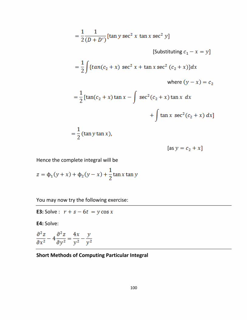
100

[Substituting

where

[as

Hence the complete integral will be

You may now try the following exercise:

E3: Solve :

E4: Solve:

Short Methods of Computing Particular Integral

101

The general method of obtaining the particular integral has been explained in

the previous section. The calculation of particular integral becomes easy, if the

function assumes the form as

We know that

…………………………………..

Similarly

……………………………………

where ….. . ..... are the derivatives of with respect to

Hence

Since is a homogeneous function of degree and so in the right

hand side of above result and have been replaced by and respectively.

In result is derived function of with respect to

being the degree of

Provided that

Working Rule:

102

From above result we can say that when is a function of

and then particular integral

is given by

is nth differential coefficient of with respect to and n is the

degree of

If we put then the desired result may be written as

Provided that

The method of obtaining particular integral in this case will be clear with the

help of following examples.

Problem 5: Solve :


or symbolically

Auxiliary equation in this case is which gives

Hence the complementary function will be

103


Where

Therefore the complete solution will be

Particular Integral of when

If then the method of obtaining particular integral discussed

above article, fails.

In such cases when it is clear that should have at least

one factor We will discuss the case when there will be only one factor

of this type and later on the obtained result will be generalized.

Let

Then particular integral corresponding to the factor will

be given by

Then

which is Lagrange’s linear equation. Hence subsidiary equations will be

104

Form first two, terms, we will obtain on integration

and from the first and last term using we get

with the help of relation we can write as

Now if the factor is repeated times, then the corresponding

particular integral will be

Working rule:

While solving questions based on this article where , students

should proceed in the following manner:

(1) Differentiate with respect to partially and multiply the expression

by , so that

(2) If is also zero, differentiate with respect to and multiply

by so that

105

Proceed in the same way as long as the derivative vanishes when

and when a stage is reached where the value can be

obtained by earlier article.

To illustrate this method ,let us take up a problem:

Problem 6: Solve :

Soltion: The given equation can be written as

or

Auxiliary equation gives

Therefore the complementary function will be

Particular integral will be obtained from

Hence the complete solution will be given by

And now a few exercise for you:

E5: Solve :

106

E6: Solve:

4.3.2 Non- Homogeneous Linear Equations

A linear partial differential equation, which is not homogeneous, may be

written as

where is not necessarily homogeneous. Had it been homogeneous then it

could be easily resolved into linear factors but now it may be reducible into linear

factors as well as may be irreducible.

We will deal with these cases separately.

Case I: Complementary Function Corresponding to Linear Factors

Suppose the non-homogeneous linear equation is written as

Right hand side being taken equal to zero for C.F.

Firstly the solution corresponding to will be obtained.

we have

or

which as the form of Lagrange’s linear equation. So subsidiary equation will

be

First and second terms produce

107

Also the first and last term yield

Hence the solution of is

By the generalization of above result it can be shown that the solution of

will be

In case there are repeated roots of the type

Then the corresponding solution can be easily obtained as

Particular Integral

In case of non- homogeneous linear equations the particular integral can be

obtained in the same way as in the case of linear equations with constant

coefficients.

Here the formulae are being given for the sake of convenience of readers.

Provided that

In case of failure

108

Provided that

In case of failure, one may write

Real part in

Similar expression will be for

Let us consider the following problems:

Problem 7: Solve:

Solution: Here the solution will consist of two parts, complementary function and

particular integral.

Complementary function will be given by

Particular integral will be

109

Thus the complete solution of the given equation will be

Problem 8: Solve :


or

Complementary function will be


110

Hence the required solution will be

Case II : When Can not be Resolved into Linear Factors

In case when is irreducible it can be factorised into linear

factors in and the method discussed in case I of obtaining the complementary

function fails. We are left with a trial solution which is usually taken and

when substituted in the given equation gives the relationship between and The

method will become clear to the readers by the following problem:

Problem 9: Solve :

Solution: Let us assume that the solution of the given equation be

that

and

Substituting these values in the given equations

Thus will be a solution of the given equation if

Putting for in the solution will be given as

Since all the values of k satisfy the given equation, so more general solution

will be given by

111

You may try the following exercise:

E 7: Solve :

E 8: Solve :

4.4 LINEAR PARTIAL DIFFERENTIAL EQUATION EQUATIONS REDUCIBLE TO

EQUATIONS WITH CONSTANT COEFFICIENTS

A differential equation having variable coefficients can sometimes by reduced

to equations with constant coefficients by suitable substitutions.

One such form is

In this case we substitute and ,

so that and

Now denoting corresponding by D and D' it can be shown that

and in general

112

These substituting reduce the equation into an equation having constant

coefficients, which can be easily solved.

We illustrate this method by the following problems:

Problem 9: Solve :

Solution: Let

or

the equation is transformed in


Problem 10: Solve :

113

Solution: Substituting


or

which is a linear equation with constant coefficients.


=

=

Thus the complete solution will be

114


E 9: Solve :

E10: Solve :

4.5 SOLUTIONS/ANSWERES

E1: The given differential equation is

Hence the auxiliary equation will be given by

which gives and

Thus the general solution will be given by

Now it has been given that the surfaces

and touch each other along the section by the plane This

condition will be used in the determination of arbitrary functions and In

other words the given condition requires that the values of p and form and

must be equal at

Calculating the values of and form , we get

115

while the values of and from are

and

equating values of p from and at , we have

at

or

To integrate we replace by , to get

Whose integral is easily obtained as

Hence,

Similarly equating q from and at , we get

at ,

or

or ,

using and noting that

Integrating,

Hence the required surface with the help of and is given

by

To evaluate it may be noted that for

116

the surface and must give the same section, . from

and from

This gives

Hence the required surface is

E2: The given equation can be written as

or symbolically

Here the auxiliary equation will be

or

which gives

Therefore the solution of the given equation will be


or

117


which gives and


Particular integral with be given by

[Substituting the value of ]

[Substituting the value of ]

Therefore the complete integral will be


118

Auxiliary equation gives



Where

Integrating by parts and then substituting the value of the particular

integral is obtained as

Therefore the complete solution will be given by

119

E5: The given equation may be written as

Auxiliary equation is which gives

Hence the complementary function is

Particular integral will be

where and

Therefore the complete solution will be

E6: Auxiliary equation in this case will be

which gives

Hence the complementary function is

120


Therefore the complete solution will be given by

E 7: The given equation can be written as

or

The complementary function will be given as


121

Therefore the required solution is

E 8: Let us assume that the solution is

then

Substituting these values in the given equation, we obtain

or

Now may be taken as and may be taken as which satisfy

the relation Thus the solution will be

122

which is satisfied for all values of α, and thus the more general solution

will be

E 9: Substituting


or

or




123

E10: Substituting and , so that


or



Particular integral

124


*****

125

UNIT 5 CALCULUS OF VARIATIONS

Structure

5.0 Introduction

5.1 Variational problem with fixed boundaries

5.2 Euler equation for functional containing First order derivative and

one independent variable

5.3 Functional dependent on higher order derivatives

5.4 Functional dependent on more than one independent variable

5.5 Variational problem in parametric form

5.6 Invariance of Eular’s equation under Coordinates Transformation

5.7 Check Your Progress: The Key

5.0 INTRODUCTION

The calculus of variation has been one of the major branches of analysis for

more than two centuries. It is a tool of great power that can be applied to a wide

variety of problems in mathematics and mathematical physics. It is primarily

concerned with the study of certain maxima and minima problems which cannot be

handled by the methods of elementary differential calculus. But in mathematical

physics we are generally encountered with the problems where one has to find the

maximal and minimal values (i.e., extreme values) of special quantities called

“functional.”

Functionals are variable quantities whose values are determined by the

choice of one or several functions. In short we may say that “functionals are

functions of functions.”

126

5.1 VARIATIONAL PROBLEM WITH FIXED BOUNDARIES

The Calculus of variations provides a method for determining maximal and

minimal values of functionals. Such problems are known as variational problems.

Before we develop a formal analysis for the calculus of variations, it may be

interesting to know that three problems of historical importance influenced the

development of this subject, which were considered and partly solved by the

ancient Greeks. The analysis was finally developed by Leonhard Euler (1707-1783) in

1744 with his discovery of the basic differential equation for maximizing curve.

Problem I: The problem of brachistochrone or the path of quickest descent.

Let and are two points in a vertical plane, but not in the

same vertical line. The question which was asked by Johann Bernoulli in 1696, was

no determine the curve, among the infinite many

possibilities, along which a bead slides under

gravity will take the shortest possible time of

descent. The common sense, as was believed

earlier, may say that the straight line joining A and B

will be the path of quickest decent as it is the

shortest distance or Galileo believed that the bead would decend more quickly

along the arc of a circle . But Bernoulli proved by an ingenious method that the path

is an arc of a cycloid. In this case although the path becomes longer but a

considerable portion of the arc will be covered at a greater speed.

Problem II: The problem of Geodesic

Geodesics are curves of shortest distance, measured along the surface,

between any two points on the surface.

In other words, we have to find a space curve

y

O x

127

Which lies on a surface such that the length s joining two

points, and , on the surface is minimum, i.e.,

is minimum.

This problem was first solved by Jakob Bernoulli in 1698. He found that the

geodesic on earth, taken as a sphere, is a smaller are of a great circle, that is, that it

lies on a plane through the centre of the sphere.

Problem III: The isoperimetric problem

The ancient Greek proposed the problem of finding the closed plane curve of given

length that encloses the largest area they called this the isoperimetric problem and

showed in a more or less rigorous manner that the obvious answer: a circle, is

correct.

Let the parametric equation of the plane curve be and if

the curve is traversed once counter clockwise as t increases from to , then the

enclosed area is given by

The problem is to maximize (find the extremum of) the functional A subject to

the condition that the length s of the given curve, i.e.,

must have a constant value.

128

General methods for solving problems with isoperimetric conditions were

handled by L. Euler.

5.2 EULER EQUATION FOR FUNCTIONAL CONTAINING FIRST ORDER

DERIVATIVE AND ONE INDEPENDENT VARIABLE

Euler-Lagrange Differential Equation for an Extremal

The calculus of variations, in the simplest form, is the method of determining

an admissible curve joining the points and such that the

integral [functional] of the variational problem,

when taken along this curve, is a maximum or a minimum ( stationary). In other

words the integral has extreme value. The curve itself often called “extremal”.

It may be noted that and and the form of the function are fixed by

given considerations, by the physics of the problem.

Remark: The unknown functions that have continuous second order

derivatives and satisfy the given boundary conditions and .

Functions of this kind are called “admissible.”

Analysis : Let and be two fixed points in the -plane and

be a curve joining and Then the integral

where is a given function of and , has a definite value for a

prescribed curve Y C

129

Now, if we vary the curve passing through the

fixed points and by some other curve through

them, the value of in general, will change and it may

happen that for some admissible curve

through these fixed points the integral has stationary

value.

Let us take one parameter family of admissible curves, say , as

close to , where is a small quantity and is an arbitrary

continuous differentiable function of , satisfying the conditions

to ensure that passes through A and B, i.e., not only are fixed but also

and

It may be noted from the adjoining figure that is called

the variation of the function and is the source of the name Calculus of variations.

If we consider the value of the integral (1) only on curves of the family

then becomes a function of and we call

The curve for which is the curve which makes stationary by

hypothesis. Therefore, the necessary condition for this is

Differentiating (4) with respect to , keeping in view that

C1

P1

A

B

P

X

130

and

we get

The stationary requirement yields

This while integrating its second term by parts, may be written as

using the boundary condition (2), it reduces to

Since is an arbitrary function subject to the condition (2), the integral (9)

can vanish for all only if

131

Hence, the curve along which the integral defined in (1), has

stationary value, must satisfy the differential equation (10),

or in short

which is called Euler’s equations or better called Euler Lagrange equation. It is a

second order non-linear differential equation.

Note : when the boundary conditions are given the solution of equation (11)

gives us only the curve for which has a stationary value it may be a

maximum or a minimum. It is only the geometry of the variational problem in many

cases may help us in deciding the nature of its extreme value.

The solutions of Euler-Lagrange equation as which are

unrestricted by the boundary conditions are called the extremals.

Other Forms of Euler’s Equations:

Form I:

Form II:

Now we shall take up few problems which will illustrate the application of

Euler-Lagrange equation.

Let us look the following problems:

132

Problem 1: On what curves can the functional

be extremized ?

Solution: Here the function under consideration is

Therefore, the Euler-Lagrange equation

for stationary value of , reduces to

This gives on integration

using the boundary conditions, we find

Therefore, an extremum can be achieved only the curve

Problem 2: [The brachistochrone problem]: Find the path on which a particle, in the

absence of friction, will slide from one fixed point to another point not in the same

vertical line in the shortest time under the action of gravity.

133

Solution: We take the origin of coordinates at one A(0

,0) of the fixed points x-axis horizontal and -axis

as downward vertical so that the particle slides from

to another fixed point not in the

P( x, y) same vertical line.

The velocity at any point on the curve

for motion of the particle under gravity is given

by

we know that the arc length is

Therefore the time taken by the particle for moving from

to is obtained from (1) and (2) as

such that

does not contain explicitly.

The functional will be stationary only when satisfies the Euler-

Lagrange equation

s

X

P(x,y)

A(0,0)

B(x1,y1) Y

134

or its corresponding form

Substituting (4) in (5), we get

or on simplification,

Separating the variables of equation (6) we may write

To integrate (7) we introduce a variable Φ by putting

so that

and

This on integration gives

Since the curve is passing through we have when

and consequently Thus

135

If we put and then equations (10) may be put in a more

recognized form

Which are the standard parametric equations of a cycloid generated by a point on

the circumference of a circle rolling along the -axis.

As stated earlier, in the geometry of the problem suggests that the time of

descent will be a minimum only. Thus the brachistochrone is a cycloid.

5.3 FUNCTIONAL DEPENDENT ON HIGHER ORDER DERIVATIVES

If the function contains higher order derivatives, say upto any order , then

then we need to extremize the integral of the form

where we consider the function differentiable times with respect to all

arguments and we assume that the boundary conditions are of the form

at the end points not only the value of the dependent variable but also of its

derivatives upto order inclusive are prescribed.

Using the same kind of analysis as we used in 5.2 and performing repeated

integration by parts, it can be shown that the required extremizing function

satisfies

136

This non-linear differential equation of order is called Euler-Poisson

equation, and its integral curves are termed extremals of the variational problem

under consideration.

Variational Problems involving several dependent variables

let us first consider a variational problem containing two dependent variables

and

we are now required to extremize the functional

for prescribed boundary conditions

That is to say that the functional is defined by the choice of the space curve

As in 5.2 we now consider one parameter family of admissible space curves as

where { is the space curve satisfying the boundary conditions, for

which is stationary, where ε is small quantity and , are arbitrary

continuous differentiable functions of satisfying the conditions

137

Now from (1)

To make stationary, we squire Therefore

Integrating the second and fourth terms by parts and using the boundary

conditions (4) at the end points, we finally get

Since this argument is applicable to any curve in a space N-

dimensions, satisfying the end points conditions

we get a system of second order non-linear differential equations

These are Euler-Lagrange equations for functionals having dependent

variables.

5.4 FUNCTIONAL DEPENDENT ON MORE THAN ONE INDEPENDENT

VARIABLES

With independent variables, we need to extremize multiple integrals of the

form

138

where z is the dependent variable.

Using the same kind of analysis as we did earlier, we find that the extermizing

function must satisfy

where stands for . This is Euler-Lagrange equation when the extremizing

curve is a functions of n independent variables.

It is also called Ostrogradsky equation.

5.5 VARIATIONAL PROBLEM IN PARAMETRIC FORM

In the investigation of certain functional

For an extremum it is sometimes more convenient to seek the solution in the

parametric form . In this case the functional reduces to the form

The corresponding Euler Lagrange equations for two dependent variable will

be

139

However, in this case these equations are not independent but one is the

consequence of the other because of the choice of the parametric representation.

For example if the arc length is taken as parameter then to the equation

we can adjoin the equation

Isoperimetric Problems and Isoperimetric Conditions [or integral side conditions]

In the strict sense of the word, as we have seen in Problem III of 5.1,

isoperimetric problems are problems in which one is required to find closed plane

curves of prescribed length (perimeter) that encloses the largest area. At present,

the term isoperimetric problem is usually extended to include the general case of

finding extremals for one integral subject to the constraints; where one or more

integral having the same integral limits and involving the same variables to take on

prescribed values, which are known as isoperimetric conditions [or integral side

conditions] are given.

Such problems are solved by the method of Lagrange multiplier parallel to the

problems studied in elementary calculus for finding out stationary values of a

function of two or more variables subject to certain constraints, which we present

here as a Lemma for a better understanding.

Lemma : Lagrange multipliers :

Suppose, we wish to determine the values that yield stationary values for

a given function where the variables are not independent but are

constrained by a side condition

140

For the extreme value of we require

Here are not independent but constrained by the condition

which gives

Multiplying (3) by an unknown number λ and adding to (2), we

get

Where λ is called Lagrange undetermined multiplier. This renders

independent and therefore for the validity of (4) we must choose λ such that

These equations together with the constraint are sufficient to

find the three unknowns λ and the values at the required stationary point.

Method of solution of the isoperimetric problem:

Let us now take up the variational problem where we wish to find the

stationary values of the functional

141

subject to the constraint that value of the functional

is held constant, and assume prescribed values at the

end points.

Following the method of Lagrange undetermined multipliers let us take a new

functional (or auxiliary functional)

Now following the analysis of 5.2 and taking

we investigate the unconstrained stationary values of at by

means of the necessary conditions

This yield the equation

Using (9), it may be written as

142

This is the Euler-Lagrange equation for isoperimetric problems, which

together with the original constraint const. and the boundary conditions, will

yield the required solution

Note: In the case of isoperimetric problems involving two or more dependent

variables, e.g. for two variables

subject to the constraint

The stationary functions must satisfy the equations

with the corresponding necessary boundary conditions.

Let us now try the following problems:

Problem 1: Find the extremals of the fuctional

with the boundary conditions

143

Solution: Here,

It contains two dependent variables and , therefore for extremals of , the

Euler-Lagrange system of equations, viz.

reduce to

Eliminating, say, from this system, we get

Its solution is easily obtained as

Now, from the first equation of the set (3)

Applying the given boundary conditions

On (4) and (5), we find

Hence the extremal is the curve of intersection of the surfaces

Let us consider another problem:

144

Problem 2: [Parametric Equation]

Show that the curve of shortest distance (geodesic) on a right circular cylinder

is a helix or a generator.

Solution: Let the parametric equations of a right circular cylinder be

Let be a curve lying on the surface of the cylinder. The length of

curve between two points and is given by the formula

The functional will be stationary only when the integrand satisfies the Euler-

Lagrange equation, viz.

This gives

On integration, we get

145

Let at then

This together with gives the parametric equation of a

helix

If then equation (2) gives const. which will correspond to a

generator of the cylinder.


E1: Find the curve of fixed length that joins the points and lies

above the -axis, and encloses the maximum area between itself and -axis.

Next, we look for transformations under which the canonical Euler equations

preserve their canonical form.

5.6 INVARIANCE OF EULAR’S EQUATION UNDER COORDINATES

TRANSFORMATION

We proved the invariance of the Euler equation

Under coordinate transformations of the form

(Such transformations change to in the original functional.) The canonical

Euler equations also have this invariance property. Furthermore, because of the

symmetry between the variables in the canonical equations, they permit

146

even more general changes of variables, i.e., we can transform the variables x,

into new variables x.

In other words, we can think of letting the transform according to their

own formulas, independently of how the variables transform. However, the

canonical equations do not preserve their form under all transformations (1). We

now study the conditions which have to be imposed on the transformations (1) if

the Euler equations are to continue to be in canonical form when written in the new

variables. i.e., if the canonical equations are to transform into new equations

Where = is some new function. Transformations of the

form (1) which preserve the canonical form of the Euler equations are called

canonical transformations.

To find such canonical transformations. We use the fact that the canonical

equations

are the Euler equations of the functional

147

In which the are regarded as 2n independent functions. We want the new

variables to satisfy the equations (2) for some function . This suggests

that we write the functional which has (2) as its Euler equations. This functional is

Where are the functions of defined by (1) and is the

derivative of thus, the functional (4) and (5) represent two different variational

problems involving the same variables and the requirement that the new

system of canonical equations (2) be equivalent to the old system (3. i.e., that it be

possible to obtain (2) from (3) by variational problems corresponding to the

functional (4) and (5) be equivalent.

Since two variational problems are equivalent (i.e., have the same externals) if

the intergrades’ of the corresponding functional differ from each other by a total

differential, which in this case means that

For some function . Thus, if a given transformation (1) from the

variables to the variables is such that there exists a function

satisfying the condition (6). Then the transformation (1) is canonical. In this case, the

function defined by (6) is called the generating function of the canonical

transformation. The function is only specified to within an additive constant.

148

Since, as is well known, a function in only specified by its total differential to within

an additive constant.

To justify the term ‘generating function.’ We must show how to actually find the

canonical transformation corresponding to a given generating function . this is

easily done. Writing (6) in the form

We find that

Then (7) is precisely the desired canonical transformation. In fact, the

equations (7) establish the connection between the old variables and the new

variables . and they also give an expression for the new Hamiltonian .

Moreover, it is obvious that (7) satisfies the condition (6), so that the transformation

(6) is indeed canonical. If the generating function does not depend on explicitly.

Then in this case, to obtain the new Hamiltonian , we need only replace

in H by their expressions in terms of

In writing (7). We assumed that the generating function is specified as a

function of x. the old variables and the new variables

It may be more convenient to express the generating function in terms of

instead . To this end, we rewrite (6) in the form

149

Thereby obtaining a new generating function

Which is to be regarded as a function of the variables Denoting (8)

by we can write the corresponding canonical

transformation in the form

Noether’s Theorem:

The system of Euler equations corresponding to the functional.

Where F does not depend on x explicitly, has the first integral

It is clear that the statement “F does not depend on explicitly” is equivalent

to the statement “F, and hence the integral (9). Remains the same if we replace by

the new variable

150

Where is an arbitrary constant.” It follows that H is a first integral of the

system of Euler equations corresponding to the functional (10) if and only if (10) is

invariant under the transformation (11).

We now show that even in the general case, there is a connection between

the existence of certain first integrals of a system of Euler equations and the

invariance of the corresponding functional under certain transformations of the

variables . We begin by defining more precisely what is meant by the

invariance of a functional under some set of transformations. Suppose we are given

a functional.

Which we write in the concise form

Where now y indicates the n-dimensional vector and ’ the n-

dimensional vector . Consider the transformation

Where The transformation (13) carries the curve y. with the

vector equation

151

Into another curve . In fact, replacing y,y in (45) by y(x), y(x), and eliminating x

from resulting n+1 equations, we obtain the vector equation

For where = .

Definition. The functional (12) is said to be invariant under the transformation (13)

i.e., if

Problem 1: The functional

is invariant under the transformation

Where is an arbitrary constant. In fact, given a curve with equation

The “transformed” curve i.e., the curve obtained from by shifting it a

distance along the x-axis, has the equation

and then

152

5.7 SOLUTIONS/ANSWERES

E1: (Restricted version of Isoperimetric Problem)

The area bounded by the arc AB,

, and the -axis is given by

Subject to the condition that the

length of the arc , say is fixed length

It is clearly necessary that has to greater than 1.

Now, the formulation of the problem is to determine the shape of the arc,

so as to maximize (1) under the isoperimetric condition (2).

We therefore, use the method of Lagrange multipliers and define a new

functional

Y

X

y=y(x)

(0,0) B(1,0)

L

153

For the stationary value of the Euler-Lagrange equation is

which is view of (5) reduce to

Integration once, we find

Solving (7) for we get

Integrating once again, in the parametric form by the substitution

and then eliminating between the forms of and , we find

which is a circle having the center as and radius and is the required curve

maximizing the enclosed area.

The constant and are given by the boundary conditions

ad the constraint

This gives

154

To get a circle of real center, from (10) it is clear that further , for admissible

values of sine function, from (11), we find

It is clear necessary that . Thus combining the three conditions, we

conclude

Because if the circular arc determined by (9) will not define as a single

valued function of . In this case the negative value of , which will correspond to

the curve below -axis will give the maximum area.

*****

Partial Differential Equation & Mechanics

Documents

Transcript of Partial Differential Equation & Mechanics