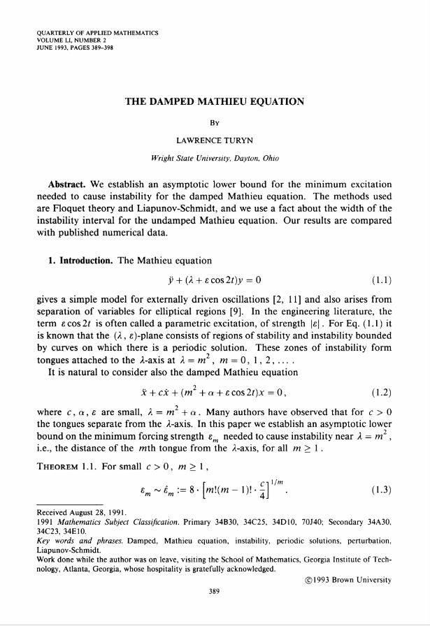
QUARTERLY OF APPLIED MATHEMATICSVOLUME LI, NUMBER 2JUNE 1993, PAGES 389-398

THE DAMPED MATHIEU EQUATION

By

LAWRENCE TURYN

Wright State University, Dayton, Ohio

Abstract. We establish an asymptotic lower bound for the minimum excitationneeded to cause instability for the damped Mathieu equation. The methods usedare Floquet theory and Liapunov-Schmidt, and we use a fact about the width of theinstability interval for the undamped Mathieu equation. Our results are comparedwith published numerical data.

1. Introduction. The Mathieu equation

y + (A + ecos2/)y = 0 (1.1)

gives a simple model for externally driven oscillations [2, 11] and also arises fromseparation of variables for elliptical regions [9], In the engineering literature, theterm ecos2? is often called a parametric excitation, of strength |e|. For Eq. (1.1) itis known that the (A, e)-plane consists of regions of stability and instability boundedby curves on which there is a periodic solution. These zones of instability formtongues attached to the A-axis at A = m , m = 0,1,2,....

It is natural to consider also the damped Mathieu equation2x + cx + (m + a + £ cos2z)x = 0, (1.2)

where c, a, e are small, A = m + a. Many authors have observed that for c > 0the tongues separate from the A-axis. In this paper we establish an asymptotic lowerbound on the minimum forcing strength sm needed to cause instability near X — m ,i.e., the distance of the mth tongue from the A-axis, for all m > 1 .

Theorem 1.1. For small c > 0, m > 1,C-il/m

m!(w- !)!•- . (1.3)em ~ :=

Received August 28, 1991.1991 Mathematics Subject Classification. Primary 34B30, 34C25, 34D10, 70J40; Secondary 34A30,34C23, 34E10.Key words and phrases. Damped, Mathieu equation, instability, periodic solutions, perturbation,Liapunov-Schmidt.Work done while the author was on leave, visiting the School of Mathematics, Georgia Institute of Tech-nology, Atlanta, Georgia, whose hospitality is gratefully acknowledged.

©1993 Brown University389

390 LAWRENCE TURYN

For c > 0, m > 1 , the vertices, i.e., the points on the mXh tongue closest to the2A-axis, are given by (A, e) ~ (m + am , ±em), where

2/m c2

m2d, := 0.

r c~\L!m C- [m!(m - 1)! - -J +-, m> 2, (M)

For concreteness, we present a few examples of Eqs. (1.3), (1.4), which can becompared with numerical results of [7, 8] for unstable solutions of the undampedMathieu equation.

The derivations of Eqs. (1.3), (1.4) are the principal results of this paper. There aremany methods for establishing perturbation results for the Mathieu equation (1.1).We will use primarily the method of Liapunov-Schmidt, i.e., alternative problems[3, 4, 6]. For the damped Mathieu equation (1.2), we begin with Liapunov-Schmidtand then draw on [1] for a crucial fact, about the "width of the instability zones" forthe undamped Mathieu equation, which is proven using the method of expansion inFourier series [9],

The heart of the argument for m > 3 is: For c = 0 , the bounding curves are givenapproximately by (a - bj mE^)2 — Pf°r a known constant pm and otherconstants b ■ m . For small c > 0, it turns out that the bounding curves are given

approximately by (a - J2jLi bj m£J)2 = p2me2m - (mc)2 , so the curves are defined for

approximately |e| > im = (rnc/pm)l/m .Approximate bounding curves for m = 1,2,3,4 are

A = 1 ± ((e/2)2 - c2)'/2,

The latter two, as well as those for m = 5 , 6, 7 , are obtained using results for c = 0[9], Approximate curves for m - 1,2,3, c = 0, .2, .4, .8 are depicted in Fig. 1.Exact curves for different values of m should not cross, so we have restricted thedomain of the curves, artificially.

2. Instability intervals and periodic solutions. First we review a basic result [10]for the undamped equation (1.1), i.e., Eq. (1.2) when c = 0.

Theorem 2.1. For every e, Eq. (1.1) has two monotonically increasing infinite se-quences of real numbers A0, A, , A2, ... and Aj, A'2 , A3, ... such that Eq. (1.1) hasa solution of period n if and only if A = An , n — 0, 1, ... , and a solution of period2n if and only if A = A^ , n — 1,2,.... The Afl and A'n satisfy

A0 < A'j < Aj < Aj < A2 < Aj < A^ < A3 < A4 <•••—> oo.

THE DAMPED MATHIEU EQUATION 391

The solutions of Eq. (1.1) are stable in the intervals (A0, A,), (k'2 , kx), (k2 , A'3),(k'4,k3),....

The proof of this result is based on properties of Hill's discriminant and its rela-tionship with the characteristic multipliers of Floquet theory. We now discuss thesethings for the more general case of Eq. (1.2).

The damped Mathieu equation (1.2), where k = m2 +. a, can be rewritten as alinear system, which is periodic with period n , so Floquet theory [6] applies. Definetwo solutions x, (t; k, e, c), x2(t; k, e, c) by the initial conditions

X[(0) = 1, Xj(0) = 0 = x2(0), x2(0) = 1.

Sometimes we will suppress dependence on k, e, c if the meaning is clear. A mon-odromy matrix

xw = (*.<*> x/;\VxiM x2(n)has trace A = x{(n) + x2(n) and characteristic multipliers

A ± \/A2 - 4e~V± = o

Here we have used the result that detX(7r) = e cn [6, Lemma III.7.3], Note that—cn

Equation (1.2) has a n (or 27r)-periodic solution if and only if one of the charac-teristic multipliers is +1 (or ±1, respectively; if a multiplier is -1 there is a In-periodic solution, which is not 7r-periodic), if and only if A = 1 +e cn (or -1 -e~cn ,respectively). Stability of x = 0 is guaranteed if |yu±| < 1 , i.e., |A| < 1 + e~'" , andinstability of x = 0 is guaranteed if |1u+| > 1 or |/z_| > 1, i.e., |A| > 1 + e~CK .Thus, for fixed c, e, the instability intervals, i.e., values of k for which x = 0 isunstable for Eq. (1.2), are bounded by the values of k for which Eq. (1.2) has a n-or 27r-periodic solution.

3. Perturbation equations and solution curves. Fix an integer m > 1 . For themethod of Liapunov-Schmidt it is convenient to use the van der Pol transformationon Eq. (1.2), considered as a system. Let

(x\ .... . ( sin ml cos mt \ ,-iy = I • I > ^(0 = I ) , z = 4/(/) y.\x \m cos mt -msmmt J

Then z satisfies

where

z = B.(t)z, (3.1)

Bx(t \ a, e, c) = - (sin2mt)A - (cos2mt)B)a

2m'+ ~ (cos 2mt)A + (sin 2mt)B)

+ ^(-2(cos2t)C - (sin(2m - 2)t + sin(2/?7 + 2)t)A

- (cos(2m - 2)t + cos(2m + 2)t)B),

392 LAWRENCE TURYN

where

Mi-0,). *-(? J)- c-(-°.J)- '-G?Note that #,(•) is ^-periodic and that the transformation, defined using 4*(-), is n-periodic (or 27r-periodic) for m = even (or m = odd, respectively). Thus, Eq. (1.2)has a ^-periodic solution if and only if Eq. (3.1) has a ^-periodic solution andm — even, and Eq. (1.2) has a 27t-periodic solution, which is not ^-periodic, if andonly if m = odd and Eq. (3.1) has either a n-periodic or 27r-periodic solution. Ofcourse, all ^-periodic solutions are also 2^-periodic.

To look for ^-periodic solutions of Eq. (3.1) we can use the method of Liapunov-Schmidt, i.e., alternative problems [3, 4, 6]. Denote by the space of func-tions f:l-»R , which are continuous and ^-periodic, with the usual norm |f| =max0<,<;r |f(f)|, and denote by Pi the mean value of f, i.e., Pi - [X/n) /0"f. Note

# 2that P : 3°n —► is a bounded linear operator, in fact, a projection: P = P.Let be the space of differentiate functions whose derivative is inderivative of f, i.e., L0f = f, and L^{a,e,c)i = /?,(•; a, e, c)i. Then L0 andL, are bounded linear operators: and L, is small if |a|, |e|, c > 0are small. The existence of a n-periodic solution of z of Eq. (3.1) is equivalent tosolving L0z = Lj(a, e , c)z, z £ , and this can be written as a system

(/ - JP)L0(a + (/ - P)z) = (/ - P)LX (a + (/ - P)z), (3.2)PL0(a + (/ - P)z) = PL] (a + (/ - P)z), (3.3)

where a = Pz e M2. The operator (I - P)L0: (/ - P)3°l -> (/ - P)3°n has a rightinverse Jf: {I — P)&>n —> (I — P. Explicitly, if f e (I-P)3°n , i.e., f is ^-periodicwith mean value zero, then there is a unique ^-periodic function z with mean valuezero such that z = f, namely, z is the unique indefinite integral of f with meanvalue zero, i.e., z = (/ - P) ft. Noting that LQP = 0 , the "auxiliary equation" (3.2)can be rewritten as

(I - P)z = 3?{I - P)L{ (a + (/ - P)z). (3.4)

Since L, = L{(a, e, c) is small for small (a, e, c), one can solve Eq. (3.4) byiteration: Let

z(0) = a, z("+l) = a + JT(/-/>)£,(a+ (/-JP)z(")), n > 0. (3.5)

We see that z n) involves aJekc , where j, k, I > 0 and j + k + I < n .The "bifurcation equations" are obtained by substituting the solution of Eq. (3.4),

(I - P)z, into Eq. (3.3) after noting that PLQ5f = 0 :

0 = PLx(a, e, c)(a + (/ - P)z) := D(a, e, c)a, (3.6)

where D(a, e, c) is a matrix. At each stage of the iteration one can substitute z"!linto Eq. (3.3) to get truncated bifurcation equations

0 = PLi{a,e,c)(a + (I - P)z(n]) := D(n\a, e, c) a, (3.7)

THE DAMPED MATHIEU EQUATION 393

where D[n\a, e, c) is a matrix. We see that D(n\a, e, c) involves a1skc , wherej, k, I > 0 and j + k +1 < n + 1. If D{n\a, e, c) contains enough terms so as tobe able to determine how many solution curves there are in the (A, e)-plane for allsmall c > 0, one can obtain approximate solutions of Eq. (3.6) from

0 = det D{n\a,e,c), (3-8„)

because D(a, e, c) = D(n){a, e, c) + + |e| + |c|)"+2), as |a| + |e| + |c| -» 0.Note that Eq. (1.2) depends on m . In effect, we are considering an infinite col-

lection of perturbation problems.For m = 1, z(0) = a, D(0\a, e, c) - -aC/2 - c//2 - eB/4 contains enough

information because Eq. (3.80) is

0=idetf ~°n a + £/2),4 \a-e/2 -c J

i.e.,2 , 2c + a —(f) •

For each small c > 0, there are two approximate solution curves a± ~2 2 1 / 2±((e/2) —c ) , defined approximately for |e/2| > c, i.e., |e| > e, ~ e, = 2c.

The scaling argument is similar to [3, pp. 435-436], The value of £[ agrees withEq. (1.3).

For m>2, e, c) = j(-aC/(2m) - cl/2) does not contain enough infor-mation; so one needs at least to iterate once in Eq. (3.5).

After some calculations one obtains

Z(1)=a + a-(-(cos2mt)A + (sin2mt)B) - (sin(2mt)A + cos(2mt)B)4 m2 4 m

s ( /cos(2m - 2)t cos(2m + 2)t+ _ (-(s,n2,)C+ ( \m_2' + ^m + 2

/sin(2m - 2)t sin(2m + 2)A\ 2m -2 + 2m + 2 )

and, after more calculations, noting that AB = C = -BA , AC = B = -CA , oneobtains

D(1\a,e,c) =

where ym = 1 if m = 2, rj = 0 if m > 3 .1 m ' I mr^Antomc pnAimh infnrmatmn Kppqucp Pn (1 ^

2 2 2 2 \-2c Ma —

For m = 2, £>(1)(a,e,c) contains enough information, because Eq. (3.8.) is2 2c a4 16 24' 16

2 2 2q_ e I £_ _?/•16 24 ^ 16

i.e.,

0 = 4c" +/ 2 2 2 >2.1 c a £~ "4 ~ 16 ~ 24

394 LAWRENCE TURYN

For each small c > 0, there are two approximate solution curves

2

24±\Jdefined for approximately |e2/16| > 2c, i.e., for |e| > e2 ~ e2 = \/32c. The valueof e2 agrees with Eq. (1.3); the corresponding value of cL = \c + c2/4 agrees withEq. (1.4).

For m > 3, D^\a,e,c) does not contain enough information. Rather thanattempt to continue the iteration in Eq. (3.5), one can use information about the"width of the instability intervals" for the undamped Mathieu equation, i.e., c = 0.In [1, 5] Fourier series are used to show that for the undamped Mathieu equation(1.1), for any m > 1 there are two solution curves, which are in (m - l)st-ordercontact at (a, e) = (0, 0). It follows that the curves must be of the form, for someconstants b- m,

Jlbj,meJ ±PmE'n> (3.10)Jj= 1

where 2pme"' is the width of the instability interval. It is known from [1] that theinstability interval has width

I IW\Q\2- l)!)2

where e = -2q in Bell's notation; hence pm = ,3m-2((|w_l),)2 • ^ follows fromEq. (3.10) that, up to a multiplicative constant k,

k det D{"'l\a, e, 0) = ~ p],/™ ■

But, since D(m ''(a, e, 0) = D[]\a, e, 0) + (terms of degrees between 3 and m),

de.D-v,., 0, = U - Y6-£r-T) -±h^A2-{tty+(3.1 r

j=3

Furthermore, since D(m~ {a, e, c) is real-analytic in c, Eq. (3.9) implies

2J ^ \ j . r\(w—0/ *-detZ) (a, e, c) = det/) (a,e,0) + —.

It follows that, to lowest order, up to a multiplicative constant, Eq. (3.9) implies

2m£ .

7 = 1

THE DAMPED MATHIEU EQUATION 395

For each small c > 0, there are two approximate solution curves2 2 m

a± ~ ^+8(J-i)+J^bj'm£j ± \ipym-{mc)2>

defined for |e| > em ~ em = {mpmc)x^m = [23m~2m({m - 1 )!)2c]I/m , which agrees

with Eq. (1.3). The corresponding value of am = e2m/(S(m2 - 1)) + c2/4 agrees withEq. (1.4).

To complete the proof of Theorem 1.1, it suffices to look for 2re-periodic solutionsof Eq. (3.1). Now let Pi = {\/2n) i. Because Bx{t\ a, s, c) only involves evenFourier terms, for all n , in Lx(a, e, c)(a + (/ - P)z1"^) the only terms of nonzeromean value over the interval 0 < t < 2n will be exactly the same as the only termsof nonzero mean value over the interval 0 < t < n , namely, constant terms obtainedfrom products of the form sin(2m-2l)t sin(2m-2/)/ or cos(2w-2/)?cos(2m-2/)/.It follows that the truncated bifurcation equations will duplicate those for the searchfor n-periodic solutions and so will not produce any new 2^-periodic solutions.

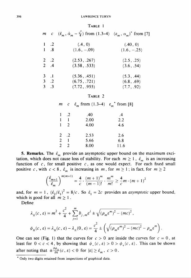
4. Comparison with numerical results. In [7, §3.6] one finds some numerical resultsfor the undamped Mathieu equation (1.1), including curves in the (A, e)-plane onwhich the characteristic multipliers ju± satisfy |/<±| = e±v , v > 0 . There is a simpleconnection between those curves and the curves in the (A, e)-plane we obtain, forfixed c > 0, for the damped Mathieu equation (1.2). This connection enables usto compare our approximate curves' vertices (am , &m) with numerical results of [7],We can also compare directly our approximate vertices with numerical results of [8]for the damped Mathieu equation.

The equations

x + cx + (A + £cos2?)x = 0, (4.1)y + (A + e cos 2t)y = 0 (4.2)

are related by y{t) = ec'^2x(t), 1 = X — c2/4. It follows that the characteristicmultipliers fix± of Eq. (4.1) are related to the characteristic multipliers ny± of (4.2) byfix±eCKl2 = n± ■ We note fiy • ny_ = 1 . We know that Eq. (4.1) has a periodic solutionif and only if |^| = 1 or \fix_\ = 1 , in which case Eq. (4.2) has a characteristicmultiplier \[iy+\ = ecx^2 or \j/_\ = eCK1/2. Since /uy+ • fiy_ = 1 , it follows that Eq. (4.1)has a periodic solution if and only if Eq. (4.2) has multipliers of magnitude e±cn^2 for"2A = A — c /4. In [7] iso-curves are in the (A, e)-plane where Eq. (4.2) has multipliersof magnitude e±cn/2. In Table 1 we give some comparisons of the vertices of thesecurves, obtained from hand measurements of the figures [7, pp. 90-92], with ourapproximate vertices in Theorem 1.1.

In [8] one finds some numerical results for the damped Mathieu equation. Again,from hand measurements of [8, Figure 1], in Table 2 we compare our results for theapproximate vertices in Theorem 1.1.

For both Tables 1, 2 we use the same units as in our paper; for example, in [8] 2yis our c and 2e is our e.

396 LAWRENCE TURYN

Table 1

m C (e"m' &m - t) fr°m (1J-4) (em > Qm)* from t7]

1 .2 (.4,0) (.40,0)1 .8 (1.6,-.09) (1.6,-.25)

2 .2 (2.53,.267) (2.5,.25)2 .4 (3.58,.533) (3.6, .54)

3 .1 (5.36,.451) (5.3,.44)3 .2 (6.75,.721) (6.8,.69)3 .3 (7.72,.955) (7.7,.92)

Table 2

m c em from (1.3-4) em* from [8]

1 .2 .40 .41 1 2.00 2.21 2 4.00 4.6

2 .2 2.53 2.62 1 5.66 6.82 2 8.00 11.6

5. Remarks. The em provide an asymptotic upper bound on the maximum exci-tation, which does not cause loss of stability. For each m > 1 , im is an increasingfunction of c, for small positive c, as one would expect. For each fixed smallpositive c, with c < 8, em is increasing in m , for m > 1 ; in fact, for m > 2

- N m(m+1) . , , ,, m m .£m+l \ 4 (W + 1) ^ 4 2em J c (m - 1)! m\ c

and, for m = 1 , (e2/e,)2 = 8/c. So e, = 2c provides an asymptotic upper bound,which is good for all m > 1 .

Define2

A±(c, e) = rn + C— + Yl,bj me] ± \/(/>mem)2 - {mcf,7=1

2<t>±{c, e) =X±(c, e) -A±(0, e) = C—± [sj(pmem)2 - (mc)2 - .

One can see (Fig. 1) that the curves for c > 0 are inside the curves for c = 0, atleast for 0 < c < 4, by showing that </>_(c, e) > 0 > <f>+{c, e). This can be shown

after noting that ±^(c, e) < 0 for |e| > sm , c > 0.

* Only two digits retained from inspections of graphical data.

THE DAMPED MATHIEU EQUATION 397

Fig. 1. c-0, c = 0.2,— c = 0.4, c = 0.8.

The characteristic exponents are \/n times the branches of the logarithm of thecharacteristic multipliers, which are complex numbers. If v denotes the real part ofa characteristic exponent, v = c/2 , then the curves in [7] of iso- v have asymptoticvertices (A, e) = (m2 + a -v2, e ), where from Eqs. (1.3) and (1.4)

em =.V

2 Jl/m

m\(m- 1)!- , am — —^—r m\(m - \)\-.v'2

2/m 2+ V ,

for m >2, and el = , dj = 0.m" — 1

The damped Mathieu equation is in some ways more akin to the undamped Math-ieu equation than it is to the damped harmonic oscillator equation x + cx + <x>2x = 0.The latter does not have oscillations, i.e., periodic solutions. Also, the latter hasdamped oscillatory solutions with "quasi-frequency" \Joj2 - c1 j4 for small c > 0;no such frequency shift occurs for the damped Mathieu equation.

References

[1] M. Bell, A note on Mathieu functions, Proc. Glasgow Math. Assn. 3, 132-134 (1957)[2] T. B. Benjamin and F. Ursell, The stability of the plane free surface of a liquid in vertical periodic

motion, Proc. Roy. Soc. London Ser. A 225, 505-515 (1954)[3] A. Canada and P. Martinez-Amores, Bifurcation in the Mathieu equation with three independent

parameters, Quart. Appl. Math. 37, 431-441 (1980)[4] Jack K. Hale, Oscillations in Nonlinear Systems, McGraw-Hill, New York, 1963[5] Jack K. Hale, On the behavior of the solutions of linear periodic differential systems near reso-

nance points, Contributions to the Theory of Nonlinear Oscillations, Ann. of Math. Stud., vol. 5,Princeton Univ. Press, Princeton, NJ, 1960, pp. 55-89

[6] Jack K. Hale, Ordinary Differential Equations, 2nd ed., Robert E. Kreiger Publ. Co., Huntington,New York, 1980

398 LAWRENCE TURYN

[7] Chihiro Hayashi, Nonlinear Oscillations in Physical Systems, Princeton Univ. Press, Princeton,NJ, 1985

[8] Th. Lieber and H. Risken, Stability of parametricallv excited dissipative systems, Phys. Lett. A129, 214-218 (1988)

[9] N. W. McLachlan, Theory and Applications of Mathieu Functions, Oxford Univ. Press, London,1947

[10] Wilhelm Magnus and Stanley Winkler, HiWs Equation, Interscience Publ., John Wiley & Sons,New York, 1966

[11] C. Pierre and E. H. Dowell, A study of dynamic instability of plates by an extended incrementalharmonic balance method, Trans. ASME Ser. E J. Appl. Mech. 52, 693-697 (1985)