Variational Quantum Evolution Equation Solver

Fong Yew Leong ∗, Wei-Bin Ewe †, and Dax Enshan Koh ‡

Institute of High Performance Computing, Agency for Science, Technology and Research (A*STAR),1 Fusionopolis Way, #16-16 Connexis, Singapore 138632, Singapore

Abstract

Variational quantum algorithms offer a promising new paradigm for solving partial differential equa-tions on near-term quantum computers. Here, we propose a variational quantum algorithm for solvinga general evolution equation through implicit time-stepping of the Laplacian operator. The use ofencoded source states informed by preceding solution vectors results in faster convergence compared torandom re-initialization. Through statevector simulations of the heat equation, we demonstrate howthe time complexity of our algorithm scales with the ansatz volume for gradient estimation and howthe time-to-solution scales with the diffusion parameter. Our proposed algorithm extends economicallyto higher-order time-stepping schemes, such as the Crank-Nicolson method. We present a semi-implicitscheme for solving systems of evolution equations with non-linear terms, such as the reaction-diffusionand the incompressible Navier-Stokes equations, and demonstrate its validity by proof-of-concept re-sults.

Keywords: Quantum computing, partial differential equations, implicit time-stepping, reaction-diffusion equa-

tions, Navier-Stokes equations

1 Introduction

Partial differential equations (PDEs) are fundamental to solving important problems in disciplines rangingfrom heat and mass transfer, fluid dynamics and electromagnetics to quantitative finance and humanbehavior. Finding new methods to solve PDEs more efficiently—including making use of new algorithmsor new types of hardware—has been an active area of research.

Recently, the advent of quantum computers and the invention of new quantum algorithms have pro-vided a novel paradigm for solving PDEs. A cornerstone of many of these quantum algorithms is theseminal Harrow-Hassidim-Lloyd (HHL) algorithm [1] for solving linear systems, which can be utilizedto solve PDEs by discretizing the PDE and mapping it to a system of linear equations. Compared toclassical algorithms, the HHL algorithm can be shown to exhibit an exponential speedup. Unfortunately,attractive as it may sound, the HHL algorithm works only in an idealized setting, and a list of caveatsmust be addressed before it can be used to realize a quantum advantage [2]. Moreover, implementingHHL and many other quantum algorithms would require the use of a fault-tolerant quantum computer,which may not be available in the near future [3]. Instead, the machines we have today are imperfect,noisy intermediate-scale quantum (NISQ) devices [4] with both coherent and incoherent errors limitingpractical circuit depths.

Over the last few years, variational quantum algorithms (VQAs) have emerged as a leading strategyto realize a quantum advantage on NISQ devices. Specifically, VQAs employ shallow circuit depths to

∗Corresponding author, leongfy@ihpc.a-star.edu.sg†ewewb@ihpc.a-star.edu.sg‡dax koh@ihpc.a-star.edu.sg

1

arX

iv:2

204.

0291

2v1

[qu

ant-

ph]

6 A

pr 2

022

optimize a cost function, expressed in terms of an ansatz with tunable parameters, through iterativeevaluations of expectation values [5]. Applications of VQAs include the variational quantum eigensolver(VQE) for finding the ground or excited states of a system Hamiltonian [6–8], the quantum approximateoptimization algorithm (QAOA) for solving combinatorial optimization problems [9], and solvers forlinear [10–12] and non-linear [13] systems of equations.

Here, we are interested in variational quantum algorithms for solving differential equations [14], suchas the Black-Scholes equation [15, 16], the Poisson equation [17, 18], and the Helmholtz equation [19].Specifically, the Poisson equation can be solved efficiently through explicit decomposition of the coefficientmatrix derived from finite difference discretization [17] using minimal cost function evaluations [18] andshallower circuit depth compared to other non-variational quantum algorithms [14, 20–22]. A naturalquestion to ask, then, is whether such variational algorithms for Poisson equations can be extendedto solving evolution equations, i.e. partial differential equations including a time domain. McArdle etal. [23] proposed a variational quantum algorithm which simulates the real (imaginary) time evolutionof parametrized trial states via forward Euler time-stepping of the Wick rotated Schrodinger equation,thereby solving the Black-Scholes equation, and by extension, the heat equation [15, 16]. Besides issuesof ansatz selection and quantum complexity, time-stepping based on an explicit Euler method may beunstable, a limiting condition exacerbated by noise.

This paper is organized as follows. In Section 2, we outline general implicit time-stepping schemesfor solving evolution partial differential equations and propose the use of a variational quantum solver toresolve the Laplacian operator iteratively. In Section 3, we apply the variational quantum algorithm tosolving a heat or diffusion equation without source terms as a proof of concept. With that, we explorepotential applications to more general evolution problems with non-linear source terms, including thereaction-diffusion (Section 4) and the Navier-Stokes equations (Section 5), where variables can be coupledthrough semi-implicit schemes.

2 Theory

Consider the second-order homogeneous evolution equation defined on the set Ω×J , where Ω ⊂ Rd denotesa d-dimensional bounded spatial domain and J = [0, T ], where T > 0 denotes a bounded temporal domain,as

∂u(~x, t)

∂t= D∇2u(~x, t) + f(~x, t), in Ω× J (1)

u(~x, 0) = u0(~x), in Ω× t = 0, (2)

where u(~x, t) is a function of spatial vector ~x and time t, D > 0 is the diffusion coefficient and f is anunspecified source term. For now, Dirichlet and Neumann boundary conditions are applicable on theboundary Γ := ∂Ω = ΓD ∪ ΓN , respectively,

u = g, in ΓD × J, (3)

∂u

∂n= 0, in ΓN × J, (4)

where ∂/∂n is the outward normal derivative on boundary Γ.For a two-dimensional rectangular domain Ω = (xL, xR)× (yL, yR) ⊂ R2, partitioning the space-time

domain Ω× J yields the space-time grid points(xij , t

k)

:=(xi, yj , t

k), i = 0, 1, . . . , nx; j = 0, 1, . . . , ny; k = 0, 1, . . . , nt, (5)

where nx, ny and nt are prescribed positive integers, such that xi = xL+i·∆x, yj = yL+j ·∆y, tk = k ·∆t,∆x = Lx/nx , ∆y = Ly/ny and ∆t = T/nt , where Lx = xR−xL and Ly = yR−yL. The discrete domaingrid is denoted by Ωd = (xi, yj) : nx ∈ 0, 1, . . . , nx, ny ∈ 0, 1, . . . , ny and boundary grid by Γd.

2

The finite difference (FD) approximation for the second-order spatial derivative (5-point) of the Lapla-cian operator taken at t = tk is

Aui,j = −δx(ui−1,j − 2ui,j + ui+1,j)− δy(ui,j−1 − 2ui,j + ui,j+1), (6)

where δx := D∆t/∆x2 and δy := D∆t/∆y2 are diffusion parameters.Using first-order FD for temporal derivative (uk+1

ij − ukij)/∆t weighted by ϑ ∈ [0, 1], the evolutionEq. (1) can be expressed in vector shorthand as

(I + ϑA)uk+1 = [I − (1− ϑ)A]uk + ∆tfk+ϑ, (7)

where I is the identity matrix of the same size, uk =[ukij

]0≤i≤nx,0≤j≤ny

and fk =[fkij

]0≤i≤nx,0≤j≤ny

.

Depending on the choice of parameter ϑ, actual time-stepping may follow an explicit (forward Euler)method (ϑ = 0), an implicit (backward Euler) method (ϑ = 1), a semi-implicit (Crank-Nicolson) method(ϑ = 1/2) or a variable-ϑ method [24]. The explicit method (ϑ = 0) is efficient for each time-step but isonly stable if it satisfies the stability condition v ≤ 1/2. The implicit (backward Euler) method (ϑ = 1)is unconditionally stable and first-order accurate in time (ε ∼ ∆t), which reads

(I +A)uk+1 = uk + ∆tfk+1. (8)

The semi-implicit Crank-Nicolson (CN) method (ϑ = 1/2) is popular as it is not only stable, but alsosecond-order accurate in both space and time (ε ∼ ∆t2), which reads(

I +A2

)uk+1 =

(I − A

2

)uk + ∆tfk+1/2 (9)

where fk+1/2 = (fk+1 + fk)/2. However, the CN method may introduce spurious oscillations to thenumerical solution for non-smooth data unless the algorithm parameters satisfy the maximum principle[25].

2.1 Variational Quantum Solver

Here, we explore a variational quantum approach towards the solution of the evolution equation (1). Inaddition to potential quantum speedup, a variational quantum algorithm could also benefit from datacompression, where a matrix of dimension N can be expressed by a quantum system with only log2Nqubits, where N is the size of the problem. Consider the Poisson equation, which is a time-independentform of Eq. (1), expressed as

−∇2u = f, in Ω ⊂ R. (10)

The Laplacian operator ∇2 in one dimension can be discretized using the finite difference method inthe x direction into an N×N coefficient matrix Ax,β as

Ax,β =

1 + αβ −1 0 · · · 0−1 2 −1 0 · · · 00 −1 2 −1 · · · 0...

. . ....

0 · · · 0 −1 2 −10 · · · 0 −1 1 + αβ

. (11)

where β ∈ D,N refers to either the Dirichlet (D) or Neumann (N) boundary condition, and αD = 1and αN = 0. This extends naturally to higher dimensions, for instance Ay,β in the y direction.

3

A variational quantum solution is to prepare a state |u〉 such that A|u〉 is proportional to a state|b〉 in a way that satisfies Eq. (10). To do that, a canonical approach [10–12] is to first decompose thematrix A over the Pauli basis Pn = P1 ⊗ · · · ⊗ Pn : ∀i, Pi ∈ I,X, Y, Z (where X = |1〉〈0| + |0〉〈1|,Y = i|1〉〈0| − i|0〉〈1|, and Z = |0〉〈0| − |1〉〈1| are the Pauli matrices and I = |0〉〈0| + |1〉〈1| is the identitymatrix) as

A =∑P∈Pn

cPP, (12)

where cP = tr(PA)/2n are the coefficients of A in the Pauli basis. Using simple operators σ+ = |0〉〈1|,σ− = |1〉〈0|, the number of terms in the decomposition can be reduced to 2 logN + 1 [17]. A moreefficient approach, however, is to express A as a linear combination of unitary transformations of simpleHamiltonians [18]. Accordingly, the decomposition of A in one dimension can be written as [19]

Ax,β = I⊗n−1 ⊗ (I −X) + S†[I⊗n−1 ⊗ (I −X) + I⊗n−10 ⊗ (X − aβI)

]S, (13)

where I0 = |0〉〈0| and β ∈ D,N, as before except here, aD = 0 and aN = 1. Here, S is the n-qubitcyclic shift operator defined as

S =

2n−1∑i=0

|(i+ 1) mod 2n〉〈i|. (14)

The expectation values of a Hamiltonian H including the shift operator S are evaluated by applyingthe unitary shift operator to the quantum state [18],

〈φ|S†HS|φ〉 = 〈φ′|H|φ′〉, (15)

where |φ〉 is an arbitrary n-qubit state and |φ′〉 = S|φ〉. Note that Eq. (13) can be re-written as

Ax,β = 2I⊗n − I⊗n−1 ⊗X︸ ︷︷ ︸H1

+S†[− I⊗n−1 ⊗X︸ ︷︷ ︸

H2

+ I⊗n−10 ⊗X︸ ︷︷ ︸H3

− bβI⊗n−10 ⊗ I︸ ︷︷ ︸H4

]S. (16)

Since expectation values of the identity operator are equal to 1, i.e. 〈φ|I⊗n|φ〉 = 〈φ′|I⊗n|φ′〉 = 1, evaluatingthe expectation value of the operator Ax,β requires only the evaluation of expectation values of the simpleHamiltonians H1−4 (H1−3 for Dirichlet boundary condition). The required number of quantum circuits istherefore limited to a constant O(n0) [18]. Similar decomposition expressions apply to problems of higherdimensions, including Ay,β in the y direction [19].

Once the matrix A is decomposed, a parameterized quantum state |ψ(θ)〉 is prepared using an ansatzrepresented by a sequence of quantum gates U(θ) parameterized by θ applied to a basis state |0〉⊗n, suchthat |ψ(θ)〉 = U(θ)|0〉⊗n. Here, we use a hardware-efficient ansatz consisting of multiple layers of RYgates across n qubits entangled by controlled-X gates (see Figure 1). For the source term f in (10), aquantum state |b〉 is prepared by encoding a real vector with the unitary Ub, such that |b〉 = Ub|0〉⊗n.Depending on the actual input, conventional amplitude encoding methods [26,27] may introduce a globalphase that must be corrected by its complex argument for computing in the real space.

With |ψ(θ)〉 and |b〉, the cost function E can be optimized in terms of A as [18]

E(r(θ), θ) = −1

2

|〈ψ(θ)|b〉|2

〈ψ(θ)|A|ψ(θ)〉, (17)

where |ψ(θ), b〉 := (|0〉|ψ(θ)〉 + |1〉|b〉)/√

2. The norm of the state vector |ψ(θ)〉 is represented by r ∈ R,where

r(θ) :=|〈ψ(θ)|b〉|

〈ψ(θ)|A|ψ(θ)〉

=|〈ψ(θ), b|X ⊗ I⊗n|ψ(θ), b〉 − i〈ψ(θ), ib|X ⊗ I⊗n|ψ(θ), ib〉|

〈ψ(θ)|A|ψ(θ)〉. (18)

4

layer 1 layer n

|0〉 Ry(θ11) • . . . Ry(θ

n1 ) •

|0〉 Ry(θ12) • . . . Ry(θ

n2 ) •

|0〉 Ry(θ13) • . . . Ry(θ

n3 ) •

......

. . ....

. . .

• •|0〉 Ry(θ

1n) . . . Ry(θ

nn)

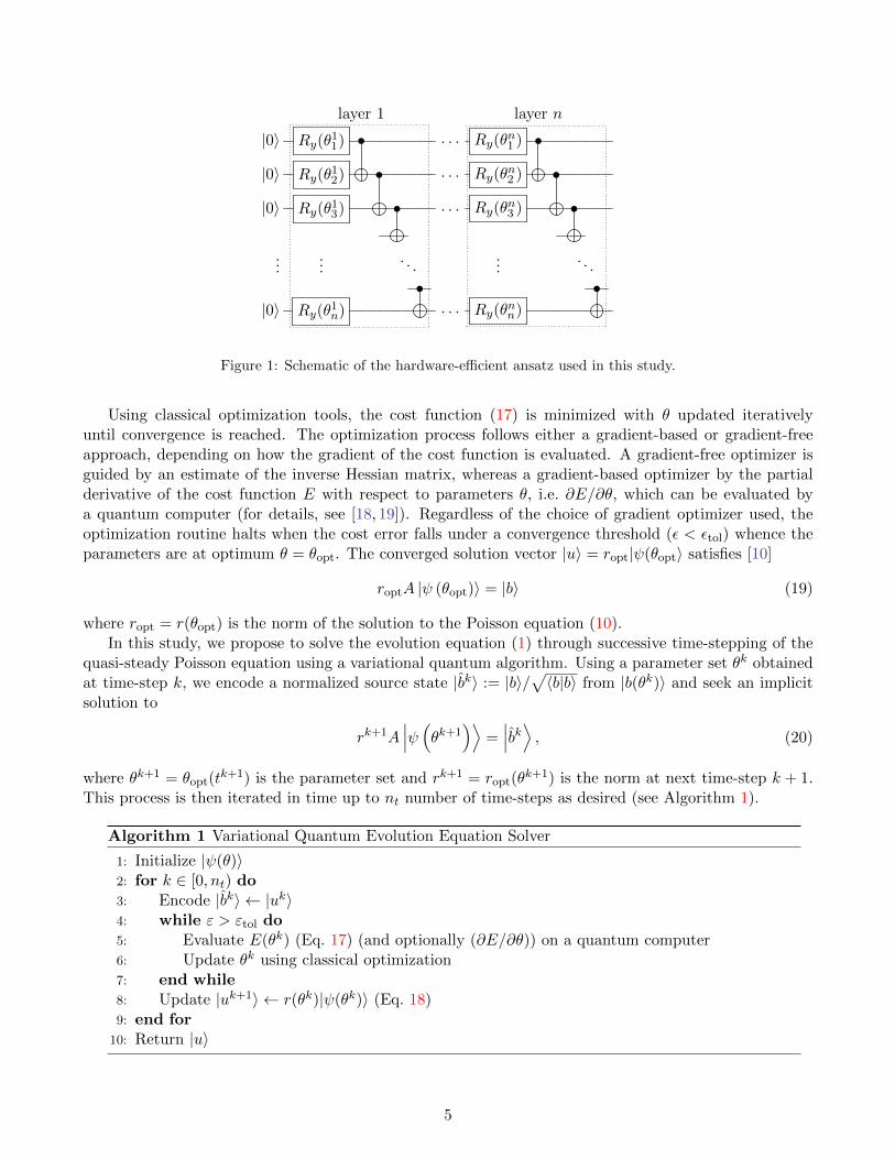
Figure 1: Schematic of the hardware-efficient ansatz used in this study.

Using classical optimization tools, the cost function (17) is minimized with θ updated iterativelyuntil convergence is reached. The optimization process follows either a gradient-based or gradient-freeapproach, depending on how the gradient of the cost function is evaluated. A gradient-free optimizer isguided by an estimate of the inverse Hessian matrix, whereas a gradient-based optimizer by the partialderivative of the cost function E with respect to parameters θ, i.e. ∂E/∂θ, which can be evaluated bya quantum computer (for details, see [18, 19]). Regardless of the choice of gradient optimizer used, theoptimization routine halts when the cost error falls under a convergence threshold (ε < εtol) whence theparameters are at optimum θ = θopt. The converged solution vector |u〉 = ropt|ψ(θopt〉 satisfies [10]

roptA |ψ (θopt)〉 = |b〉 (19)

where ropt = r(θopt) is the norm of the solution to the Poisson equation (10).In this study, we propose to solve the evolution equation (1) through successive time-stepping of the

quasi-steady Poisson equation using a variational quantum algorithm. Using a parameter set θk obtainedat time-step k, we encode a normalized source state |bk〉 := |b〉/

√〈b|b〉 from |b(θk)〉 and seek an implicit

solution to

rk+1A∣∣∣ψ (θk+1

)⟩=∣∣∣bk⟩ , (20)

where θk+1 = θopt(tk+1) is the parameter set and rk+1 = ropt(θ

k+1) is the norm at next time-step k + 1.This process is then iterated in time up to nt number of time-steps as desired (see Algorithm 1).

Algorithm 1 Variational Quantum Evolution Equation Solver

1: Initialize |ψ(θ)〉2: for k ∈ [0, nt) do3: Encode |bk〉 ← |uk〉4: while ε > εtol do5: Evaluate E(θk) (Eq. 17) (and optionally (∂E/∂θ)) on a quantum computer6: Update θk using classical optimization7: end while8: Update |uk+1〉 ← r(θk)|ψ(θk)〉 (Eq. 18)9: end for

10: Return |u〉

5

In this study, the variational quantum algorithm is implemented in Pennylane (Xanadu) [28] using astatevector simulator with the Qulacs [29] plugin as a backend for quantum simulations, and the L-BFGS-B optimizer for parametric updates. Amplitude encoding is carried out via the standard Mortonnen statepreparation template [30] with custom global phase correction. For hardware emulation via the QASMsimulator (Qiskit), we refer the reader to the excellent cost-sampling analysis of Sato et al. [18].

3 Applications to the Heat/Diffusion Equation

Consider the following one-dimensional heat or diffusion equation without a source term

∂u

∂t= D

∂2u

∂x2, in Ω× J (21)

u = u0(x), in Ω× t = 0. (22)

Dirichlet conditions are applied on the boundaries of a 1D domain Ω = (xL, xR) ⊂ R, where u(xL, t) =gL(t) and u(xR, t) = gR(t), such that the boundary vector uD = (gL, 0, . . . , 0, gR) is known for all t.

To solve Eq. (22), the variational quantum evolution algorithm (Algorithm 1) can be employed witha suitable time-stepping scheme (7). For the implicit Euler (IE) method (8), the matrix A and sourcestate |b(θk)〉 can be decomposed into

A = I⊗n + δxAx,D,

|bk〉 = |uk〉+ δx|uk+1D 〉,

(23)

where |uk〉 = rk|ψ(θk)〉.

For the Crank-Nicolson (CN) method (9), it follows that the Auk term, which carries a small but non-trivial evaluation cost, can be eliminated using the source state of the previous time-step k − 1, leadingto

A = 2I⊗n + δxAx,D,

|bk〉 = 4|uk〉 − 2δx

(|bk−1〉+ |uk+1/2

D 〉).

(24)

where 2∣∣∣uk+1/2D

⟩:=(∣∣∣uk+1

D

⟩+∣∣ukD⟩). Here, the presence of a k− 1 term in

∣∣bk−1⟩ is not unexpected due

to temporal finite differencing at second-order accuracy.For a space-time domain Ω×J ∈ [0, 1]× [0, 1], let the number of time-steps be nt = 20 and the spatial

intervals be nx = 2n + 1, where n is the number of qubits, and δx = 1 is the diffusion parameter. Weemploy the Dirichlet boundary condition with boundary values (gL, gR) = (1, 0) and initial values u0 = ~0.With initial random parameters θ0 ∈ [0, 2π], we run a limited-memory Broyden-Fletcher-Goldfarb-Shannoboxed (L-BFGS-B) optimizer [31–34] to optimize θ with absolute and gradient tolerances set at 10−8.

Figure 2a compares solutions obtained from the variational quantum solver (23) and classical methodsto a 1D heat or diffusion problem in time-increments of 0.1, where the number of qubits and ansatz layersexpressed as a set n-l, are 3-3 and 4-4. Here we define the time-averaged trace error εtr as

εtr :=1

nt

nt−1∑k=0

√1− |〈ψ (θk)| uk〉 |2, (25)

where∣∣uk⟩ :=

∣∣uk⟩ /√〈uk | uk〉 is the normalized classical solution vector at time k. The trace errors ofsolutions shown in Figure 2a are 0.0008 and 0.0025 for n-l sets of 3-3 and 4-4 respectively.

Figure 2b shows how the cost function E depends on the number of optimization steps for n-l of 3-3and 4-4 (10 sampled runs each). Each distinct step in E represents sequential optimization from solution|ψ(θk)〉 at time-step k towards the solution |ψ(θk+1)〉 at k + 1. For small time-step ∆t, θk provides agood initial parameter set for solving optimization step k+ 1. If the ansatz parameters were re-initializedrandomly θk ∈ [0, 2π] before each time-step, significantly more optimization steps would be required onaverage for convergence for each run (see Fig. 2b, inset).

6

Figure 2: (a) Implicit variational quantum solutions to a 1D heat conduction or diffusionproblem in time-increments of 0.1, with boundary values gL, gR = 1, 0, initial valuesu0 = 0 and diffusion parameter δx = 1. (Left) Qubit–layer count n-l = 3-3 and time-averaged trace error εtr = 0.0008; (Right) n-l = 4-4, εtr = 0.0025. (b) Cost functionvs. number of optimization steps for 10 runs. Inset: Input parameters are re-initializedrandomly, θ ∈ [0, 2π], before each time-step for 5 runs.

7

3.1 Time complexity

Here we briefly examine the time complexity of the quantum algorithm excluding the classical computingcomponents. Following the analysis of the variational Poisson solver [18], the time complexity of theproposed variational evolution equation solver per time-step reads

T ∼ O(Teval

(l + e+ n2

ε2

)), (26)

where the terms within the inner parentheses indicate the time complexity of the state preparation scalingas O(l+e+n2), which consists of the ansatz depth l, the encoding depth O(n2) [35], and the depth O(n2)of the circuit needed to implement the n-qubit cyclic shift operator, and that of the number of shotsO(ε−2) required for estimation of expectation values up to a mean squared error of ε2. The requirednumber of quantum circuits depends on the boundary conditions applied (3 for periodic, 4 for Dirichletand 5 for Neumann conditions), scaling only as O(n0). Teval is the time-averaged number of functionevaluations,

Teval :=1

nt

nt−1∑k=0

Teval, (27)

where Teval is the sum of function evaluations required for a run with nt time-steps. Using a gradient-basedoptimizer, the time complexity for gradient estimation via quantum computing would scale as the ansatzvolume O(nl) representing the number of quantum circuits required for parameter shifting. Otherwise,with a gradient-free optimizer, the time complexity simply contributes towards Teval as additional functionevaluations required to evaluate the Hessian for gradient descent.

To see if the time complexity for gradient-free optimization scales as O(nl), we plot the time-averagednumber of function evaluations Teval against the number of parameters nl (Fig. 3a). Indeed, we found thatTeval scales reasonably with nl (see trendline of slope 1), despite apparent tapering at higher l. Fig. 3bshows that the time-averaged trace error εtr decreases with circuit depth l, even for over-parameterizedquantum circuits where the number of layers exceeds the minimum required for convergence, lmin := 2n/n[36]. For low grid resolution n = 3, the trace error is limited to a minimum of ∼ 10−4.

For deep and wide quantum circuits, the increase in optimization time is exacerbated by the presenceof barren plateaus, or vanishingly small gradients in the energy landscape, where re-initialization can leaveone trapped at a position far removed from the minimum [37–39]. Conversely, short time-steps lead toefficient solution trajectories that remain close to the local cost minima, leading to significant reductionin optimization times. To verify this, we conduct numerical simulations varying the diffusion parameterδ with l = n up to time T = 1. Figure 3c shows that the number of iterations, or required optimizationsteps, per time-step increases linearly with δ. Close inspection of the time-averaged trace distance showsbimodal distributions at higher δ, which separates success and failure during convergence towards theglobal minimum (see Fig. 3d, dotted lines), resembling local minima traps due to poor optimization orexpressivity of ansatze [19,40].

3.2 Discretization error

Time evolution can be at a higher order, specifically for the Crank-Nicolson method. The problemstatement is identical to the previous one, except with Dirichlet boundary values (gL, gR) = (0, 0) and theinitial condition u0 = sin(πx/Lx), where we use Lx = 1 as the spatial length of the domain. This admitsan exact analytical solution,

u(x, t) = sin

(πx

Lx

)exp

[−Dt

(π

Lx

)2]. (28)

8

Figure 3: Logarithmic plots of time-averaged (a) number of function evaluations Tevalvs. number of parameters nl, (b) trace error εtr vs. number of layers l, (c) number ofiterations T and (d) trace error εtr vs. diffusion parameter δ for l = n up to T = 1. Eachdata point and error bar represents, respectively, the mean and standard deviation outof 25 runs.

9

Figure 4: Variational quantum solutions to a 1D heat conduction or diffusion problem forqubit-layers (a) n-l = 3-3 and (b) n-l = 4-4 in time-increments of 0.1 using implicit Eulerand Crank-Nicolson schemes, with Dirichlet boundary values (gL, gR) = (0, 0), initialvalues u0 = sin (πx) and diffusion parameter δx = 1. Dashed lines denote exact solutions.

Figure 4 compares variational quantum and exact solutions using implicit Euler and Crank-Nicolson (CN)schemes. The discretization error for the higher-order CN scheme is reduced significantly, especially atlower grid resolution (n = 3). Although the complexity costs for both methods (23) and (24) are similar,note however that the CN method may introduce spurious oscillations for non-smooth data [24], an issuewhich may be exacerbated by quantum noise [41].

3.3 Higher dimensions

The preceding analysis can be extended to higher dimensions. Consider the following two-dimensionalheat or diffusion equation in Ω× J , where Ω = (xL, xR)× (yL, yR) ⊂ R2:

∂u

∂t= D

(∂2u

∂x2+∂2u

∂y2

), in Ω× J, (29)

u = u0, in Ω× t = 0. (30)

Under the implicit Euler scheme (8), the matrix A and source state |bk〉 can be decomposed into

A = I⊗n + δxAx,D + δyAy,D,∣∣∣bk⟩ =∣∣∣uk⟩+ δx

∣∣∣uk+1x,D

⟩+ δy

∣∣∣uk+1y,D

⟩.

(31)

Dirichlet conditions are applied on the boundaries, where u(xL,R, y, t) = gxL,R(y, t) and u(x, yL,R, t) =gyL,R(x, t). Let the number of spatial grid intervals be nx = 2mx + 1 and ny = 2my + 1, where mx is thenumber of qubits allocated to the x grid, my to the y grid, and n = mx + my is the total number ofqubits. Accordingly, A is decomposed in terms of simple Hamiltonians in x and y as

Ax,β = 2I⊗n − I⊗n−1 ⊗X︸ ︷︷ ︸H1

+

S†[0,mx)

[− I⊗n−1 ⊗X︸ ︷︷ ︸

H2

+ I⊗myI⊗mx−10 ⊗X︸ ︷︷ ︸H3

− bβI⊗myI⊗mx−10 ⊗ I︸ ︷︷ ︸H4

]S[0,mx), (32)

10

Figure 5: (a) Contour solution plot of 2D heat conduction or diffusion problem at timeT = 1 on a 8× 8 x-y square grid (qubit-layer mx-my-l = 3-3-6) with Dirichlet boundary

values (gxL, gxR

) = (0, 0) and (gyL, gyR

) = (1, 0), initial values u0 = ~0, nt = 20 anddiffusion parameters δx = δy = 1. (b) Solution vectors in time-increments of 0.1.

Ay,β = 2I⊗n − I⊗my−1 ⊗X ⊗ I⊗mx︸ ︷︷ ︸H1

+

S†[mx,n)

[− I⊗my−1 ⊗X ⊗ I⊗mx︸ ︷︷ ︸

H2

+ I⊗my−10 ⊗X ⊗ I⊗mx︸ ︷︷ ︸

H3

− bβI⊗my−10 ⊗ I⊗mx+1︸ ︷︷ ︸

H4

]S[mx,n), (33)

where H1−4 are simple Hamiltonians to be evaluated (H1−3 for Dirichlet boundary condition).Figure 5 shows solution snapshots to a 2D heat conduction or diffusion problem taken at time T = 1

with Dirichlet boundary values (gxL , gxR) = (0, 0) and (gyL , gyR) = (1, 0), initial values u0 = ~0, nt = 20and diffusion parameters δx = δy = 1. Results obtained from variational quantum solver agree withclassical solutions with time-averaged trace errors of up to 10−2.

4 Applications to the Reaction-Diffusion Equations

Here, we extend applications of our variational quantum solver to evolution equations with non-trivialsource terms. Consider a two-component homogeneous reaction-diffusion system of equations

∂u(~x, t)

∂t= D∇2u(~x, t) + f(~x, t), in Ω× J, (34)

u(~x, 0) = u0(~x), in Ω× t = 0, (35)

where u = [u1, u2]T is a concentration tensor, D = diag[D1, D2]

T is a diffusion tensor and f = [f1(u1, u2),f2(u1, u2)]

T is a coupled reaction source term. First proposed by Turing [42], the reaction-diffusionequations are useful for understanding pattern formation and self-organization in biological and chemicalsystems [43,44], such as morphogenesis [45] and autocatalysis [46].

Here, we propose a semi-implicit time-stepping scheme, whereby the coupled, non-linear source termis solved at the current time-step k. With explicit source term fk, the implicit Euler scheme (8) reads

(I +A)uk+1 = uk + ∆tfk. (36)

11

The two-component tensor A = [A1, A2]T and source state b = [b1, b2]

T can then be decomposed into

A = I⊗n + δxAx,D,∣∣∣bk⟩

=∣∣∣uk⟩

+ δx

∣∣∣uk+1D

⟩+ ∆t

∣∣∣fk⟩ , (37)

where δx = 22n∆tD is the two-component diffusion parameter vector. With a linear Hermitian sourcematrix f , a fully implicit time-stepping scheme becomes available (Appendix A).

4.1 Implementation

The semi-implicit variational quantum solver solves for the Laplacian for each component using a quantumcomputer and the solution vectors are explicitly coupled through source terms prior to re-encoding inpreparation for the next time-step (see Algorithm 2).

Algorithm 2 Variational Quantum Solver for Reaction-Diffusion Equations (Semi-implicit)

Initialize |ψ〉(θi) for each component i2: for k ∈ [0, nt) do

Encode |bk〉 ← |uk〉 (Eq. 37)4: while εi > εtol do

Evaluate Ei(θki ) on a quantum computer

6: Update θki using classical optimizationend while

8: Update |uk+1〉 ← r(θk)|ψ(θk)〉end for

10: Return |u〉

4.2 1D Gray-Scott Model

The Gray-Scott model [46] was originally conceived to model chemical reactions of the type U+2V → 3V ,V → P , where U , V and P are chemical species with reaction term

f(u) =

[k1(1− u1)− u1u22−(k1 + k2)u2 + u1u

22

], (38)

where k1 and k2 are kinetic rate constants.An interesting class of Gray-Scott solutions involves periodic splitting of chemical wave pulses [24,47].

Here, we conduct a pulse splitting numerical experiment under limited spatial and temporal resolutions,using input parameters D = [10−4, 10−6]T , k1 = 0.04 and k2 = 0.02, with a mid-pulse initial conditionand Dirichlet boundary conditions as

u1(x, 0) = 1− 1

2sin100(πx), u2(x, 0) =

1

4sin100(πx), x ∈ (0, 1), (39)

u1(0, t) = u1(1, t) = 1, u2(0, t) = u2(1, t) = 0, t ∈ [0, T ], (40)

where time t extends up to T = 600 on dt = 0.5.Figure 6a shows how an initial mid-pulse can spontaneously and periodically split in space and time,

a phenomenon captured using variational quantum diffusion reaction solver (see Algorithm 2) even onrelatively low spatial resolutions.

12

Figure 6: Space-time solutions of (a) mid-pulse wave-splitting in 1D two-component Gray-Scott model obtained using semi-implicit variational quantum reaction-diffusion solveron 26 = 64 grid points up to T = 600, for chemical species u1 (left) and u2 (right).Parameters include D = [10−4, 10−6]T , k1 = 0.04, k2 = 0.02 and dt = 0.5. (b) Travelingwave solutions for 1D Brusselator model on 24 = 16 grid points up to T = 400 onNeumann boundary conditions. Parameters include D = [10−4, 10−4]T , k1 = 3, k2 = 1and dt = 0.5.

13

4.3 1D Brusselator Model

So far, we have been looking at only Dirichlet boundary conditions. Here, we demonstrate a test examplefor Neumann boundary conditions in a diffusion-reaction model, namely, the Brusselator model [48], whichwas developed by the Brussels school of Prigogine to model the behavior of non-linear oscillators in achemical reaction system. The model reaction term reads

f(u) =

[−(k1 + 1)u1 + u21u2 + k2

k1u1 − u21u2

]. (41)

Using D = [10−4, 10−4]T , k1 = 3 and k2 = 1, with initial conditions

u1(x, 0) =1

2, u2(x, 0) = 1 + 5x, x ∈ (0, 1), (42)

∂u1∂x

(0, t) =∂u1∂x

(1, t) = 0,∂u2∂x

(0, t) =∂u2∂x

(1, t) = 0, t ∈ [0, T ], (43)

where time t extends up to T = 400 on dt = 0.5.Figure 6b shows how a chemical pulse can be spontaneously created, which continually travels leftwards

in time, creating traveling waves that appear as striped patterns in time despite low spatial resolutions.

5 Applications to the Navier-Stokes Equations

The Navier-Stokes equations are a set of non-linear partial differential equations that describes the motionof fluids across continuum length scales. There are several studies aimed at applying quantum algorithmsto computational fluid dynamics (see review [49]), ranging from reduction of partial differential equationsto ordinary differential equations [50] and quantum solutions of sub-steps of the classical algorithm [51,52]to the quantum Lattice Boltzmann scheme [53].

Here, we look into the potential use of variational quantum algorithms to evolve the fluid momentumequations in time. Consider the incompressible Navier-Stokes equations in non-dimensional form

∂u

∂t+ u · ∇u = −∇p+

1

Re∇2u, (44)

∇ · u = 0, (45)

where u is the velocity vector and p is the fluid pressure. The ratio Re = UcLc/ν is the Reynoldsnumber, where Uc is the characteristic flow velocity across a characteristic length-scale Lc and ν is thefluid kinematic viscosity.

Unlike other temporal evolution equations, the incompressible Navier-Stokes equations cannot be time-marched directly as the resultant velocities do not satisfy the continuity constraint (45), and hence arenot divergence-free. To resolve this, the projection method [54], also known as the predictor-corrector orfractional step method, separates the solution time-step into velocity and pressure sub-steps, also knownas the predictor and corrector steps.

5.1 Projection method

5.1.1 Predictor step

The predictor step first approximates an intermediate velocity u∗ by solving the fluid momentum equation(44) in the absence of pressure, i.e. the Burgers’ equations [55], of the form(

1− ∆t

Re∇2

)u∗ =

(1−∆tuk∇·

)uk. (46)

14

Through a semi-implicit scheme, the viscous terms are handled implicitly using the variational quan-tum evolution equation solver and the non-linear inertial terms explicitly as source terms using classicalcomputation. For quantum algorithms for non-linear problems, the reader is referred to separate workson quantum ordinary differential equation solvers [50, 55], Carleman linearization [56] and a variationalquantum nonlinear processing unit (QNPU) [13].

On a two-dimensional domain with Dirichlet boundary conditions, the tensor Au = [Au, Av]T and

source state bu = [bu, bv]T can be decomposed as

Au = I⊗n + δxAx,D + δyAy,D,

|bku〉 = (1−∆tFk)|uk〉+ δx|uk+1

x,D 〉+ δy|uk+1y,D 〉,

(47)

where δx := ∆t/(Re∆x2) and δy := ∆t/(Re∆y2). F k = DkuBx,D + Dk

vBy,D is an operator which ap-proximates the non-linear inertial term, where Dk

u are diagonal matrices with velocity vectors |uk〉 alongthe diagonals and B is a divergence matrix discretized through center differencing, for instance in the xdirection, as

Bx,β =1

2∆x

αβ 1 0 · · · 0−1 0 1 0 · · · 00 −1 0 1 · · · 0...

. . ....

0 · · · 0 −1 0 10 · · · 0 −1 αβ

. (48)

where β ∈ D,N refers to either Dirichlet (D) or Neumann (N) boundary condition. Here, αD = 0 andαN = −1.

5.1.2 Corrector step

The second corrector step solves for the velocity uk+1 by correcting the intermediate velocities u∗ usingthe pressure gradient as a Lagrange multiplier to enforce continuity. Applying divergence to the correctionequations yields the pressure Poisson equation for the pressure field at half-step

−∇2pk+1 = − 1

∆t∇ · u∗, (49)

which can be solved implicitly in two dimensions (x, y) via the following decomposition:

Ap =∆t

∆x2

(Ax,N +

1

2I⊗n0

)+

∆t

∆y2

(Ay,N +

1

2I⊗n0

),

|bkp〉 = −(Bx,D|u∗〉+By,D|v∗〉).(50)

Note the addition of a simple Hermitian I0 = |0〉〈0| to the pressure matrix Ap, which would otherwise besingular (corank 1) under Neumann boundary conditions for the pressure field.

With the new pressure pk+1, the velocities are updated at the k + 1 time-step as

uk+1 = u∗ −∆tBN|pk+1〉, (51)

where BN = [Bx,N , By,N ]T are the gradient operators.

15

5.2 Implementation

Overall, the variational quantum solver for Navier-Stokes equations using the projection method (seeAlgorithm 3) involves two sequential steps, the first requiring a number of Algorithm 1 iterations equalto the number of velocity components, and the second for the pressure Poisson step. For two-dimensionalflows, the number of velocity components to be solved can be effectively reduced by one through the vor-ticity stream-function formulation (Appendix B). In computational fluid dynamics, these implicit systemsof linear equations are often the most computationally expensive parts to solve in classical algorithms,providing incentives for potential speedup via quantum computing [49,52].

Algorithm 3 Variational Quantum Navier-Stokes Equation Solver (Projection Method)

Initialize |ψ(θ)〉 for u, pfor k ∈ [0, nt) do

3: Encode |bku〉 ← |uk〉 (Eq. 47)

while εu > εtol doEvaluate E(θku) on a quantum computer for Au and |bk

u〉6: Update θku using classical optimization

end whileUpdate |u〉∗ ← r(θku)|ψ(θku〉)

9: Encode |bkp〉 ← |u〉∗ (Eq. 50)while εp > εtol do

Evaluate E(θkp) on a quantum computer for Ap and |bkp〉12: Update θkp using classical optimization

end whileUpdate |pk+1〉 ← r(θkp)|ψ(θkp)〉

15: Update |uk+1〉 ← |u∗〉, |pk+1〉end forReturn |u〉, |p〉

5.3 2D Cavity Flow

The lid-driven cavity flow is a standard benchmark for testing incompressible Navier-Stokes equations [57].Consider a two-dimensional square domain Ω = (0, L)×(0, L) ⊂ R2 with only one wall sliding tangentiallyat a constant velocity. For simplicity, we employ a fixed collocated grid, instead of a staggered grid whichhelps avoid spurious pressure oscillations but at the cost of increased mesh and discretization complexity.No-slip boundary conditions apply on all walls, so that zero velocity applies on all wall boundaries exceptone moving at u(x, 0) = 1.

Figure 7a shows a snapshot of a test case conducted on a 2n = 8 × 8 grid at ∆t = 0.5 up to T = 5,with the central vortex shown by normalized velocity quivers in white. In terms of time complexity, wenote that the pressure correction step requires a greater number of function evaluations for convergencecompared to an implicit velocity step (Fig. 7b). This is due to the additional quantum circuits forevaluating the H4 Hamiltonians (32, 33) for Neumann boundary conditions and one for specifying thereference pressure (50), leading to a total of 9 evaluation terms compared to 6, a ratio which corroborateswith the apparent ∼ 50% increase in function evaluations shown in Fig. 7b.

While not directly comparable to classical computational fluid dynamics in numerical accuracy, thisexercise, nevertheless, roadmaps potential applications of the variational quantum method towards morecomplicated flow problems [52].

16

Figure 7: (a) 2D lid-driven cavity flow (Re = 100) on a 2n = 8× 8 grid at ∆t = 0.5 up toT = 5 and upper boundary sliding in the x direction at u(x, 0) = 1. Color map indicatesvelocity magnitude with normalized velocity quivers in white indicating direction of flow.(b) Plots of cumulative number of function evaluations vs. time for intermediate velocities(u,v) and pressure (p).

6 Conclusion

In this study, we proposed a variational quantum solver for evolution equations which include a Laplacianoperator to be solved implicitly. For short time-steps ∆t, the use of initial parameter sets encoded fromprior solution vectors results in faster convergence compared to random re-initialization. The overalltime complexity scales with the ansatz volume O(nl) for gradient estimation and with the number oftime-steps O(nt) for temporal discretization. Our proposed algorithm extends naturally to higher-ordertime-stepping and higher dimensions. For evolution equations with non-trivial source terms, the semi-implicit scheme can be applied, where non-linear source terms are handled explicitly. Using statevectorsimulations, we demonstrated that variational quantum algorithms can be useful in solving popular partialdifferential equations, including the reaction-diffusion and the incompressible Navier-Stokes equations.

The present work aims at bridging the gap between variational quantum algorithms and practicalapplications. Our work has assumed that the state preparations, unitary transformations and measure-ments are implemented perfectly, and does not consider the effects of quantum noise from actual hardwareor any potential amplification from iterative time-stepping. In our implementation, we only consideredthe hardware-efficient ansatz with Ry rotation gates and controlled-NOT entanglers, and thus leave openthe question about the performance of other ansatzes. Future work can include noise mitigation [58–60],ansatz architecture, non-linear algorithms and cost-efficient encoding.

Acknowledgements

We thank Maria Schuld for helpful comments on amplitude embedding. This work was supported inpart by the Agency for Science, Technology and Research (A*STAR) under Grant No. C210917001.DEK acknowledges funding support from the National Research Foundation, Singapore, through GrantNRF2021-QEP2-02-P03.

17

A Fully implicit scheme for linear Hermitian source term

For a reaction-diffusion system of equations with non-trivial source terms 35, time-stepping could berendered fully implicit if the source terms can be expressed as a linear Hermitian matrix with constantcoefficients. Consider a two-component 1D chemical reaction with source terms of the form

f(u) =

[k11 k12k21 k22

]⊗ I

[u1u2

], (A.1)

where kij (i, j ∈ 1, 2) are kinetic rate constants that are components of the linear Hermitian matrixK = KT ∈ RN×N , whose off-diagonal elements are equal, i.e. k12 = k21; I is the identity matrix of sizeN ×N and [u1, u2]

T is a concentration vector of length 2N . This problem requires n + 1 qubits, wheren = log2N . Following the implicit Euler scheme (Eq. 8), we set up a 2N × 2N coefficient matrix, whichdecomposes as

A = I⊗n+1 + δxI ⊗Ax,β −∆t (k11I0 + k22I1 + k12X)⊗ I⊗n, (A.2)

where Ax,β is the discretized N × N coefficient matrix for a single component (Eq. 16) containing upto four Hamiltonian terms H1−4. Note the last three additional Hamiltonian terms contributed by thesource term.

B Vorticity stream-function formulation

For two-dimensional incompressible flows, the vorticity stream-function formulation can be used to elim-inate the pressure as a dependent variable, such that

∂ω

∂t+ u

∂ω

∂x+ v

∂ω

∂y=

1

Re

(∂2ω

∂x2+∂2ω

∂x2

), (B.1)

∂2ψ

∂x2+∂2ψ

∂x2= −ω, (B.2)

where ω = ∂v/∂x − ∂u/∂y is the flow vorticity and the stream-function ψ satisfies u = −∂ψ/∂y andv = ∂ψ/∂x. It follows that the re-formulation u, v, p → ω, ψ can simplify the variational quantumalgorithm 3 by reducing the number of velocity components by one, at the cost of specifying stream-function values along the domain boundaries.

References

[1] Aram W. Harrow, Avinatan Hassidim, and Seth Lloyd. Quantum algorithm for linear systems ofequations. Phys. Rev. Lett., 103:150502, Oct 2009.

[2] Scott Aaronson. Read the fine print. Nature Physics, 11(4):291–293, 2015.

[3] Kishor Bharti, Alba Cervera-Lierta, Thi Ha Kyaw, Tobias Haug, Sumner Alperin-Lea, AbhinavAnand, Matthias Degroote, Hermanni Heimonen, Jakob S. Kottmann, Tim Menke, Wai-Keong Mok,Sukin Sim, Leong-Chuan Kwek, and Alan Aspuru-Guzik. Noisy intermediate-scale quantum algo-rithms. Rev. Mod. Phys., 94:015004, Feb 2022.

[4] John Preskill. Quantum computing in the NISQ era and beyond. Quantum, 2:79, 2018.

[5] M. Cerezo, Andrew Arrasmith, Ryan Babbush, Simon C. Benjamin, Suguru Endo, Keisuke Fujii,Jarrod R. McClean, Kosuke Mitarai, Xiao Yuan, Lukasz Cincio, and Patrick J. Coles. Variationalquantum algorithms. Nat Rev Phys, 3:625–644, sep 2021.

18

[6] Alberto Peruzzo, Jarrod McClean, Peter Shadbolt, Man-Hong Yung, Xiao-Qi Zhou, Peter J Love,Alan Aspuru-Guzik, and Jeremy L O’Brien. A variational eigenvalue solver on a photonic quantumprocessor. Nature communications, 5(1):1–7, 2014.

[7] Jarrod R McClean, Jonathan Romero, Ryan Babbush, and Alan Aspuru-Guzik. The theory ofvariational hybrid quantum-classical algorithms. New Journal of Physics, 18(2):023023, 2016.

[8] Abhinav Kandala, Antonio Mezzacapo, Kristan Temme, Maika Takita, Markus Brink, Jerry M Chow,and Jay M Gambetta. Hardware-efficient variational quantum eigensolver for small molecules andquantum magnets. Nature, 549(7671):242–246, 2017.

[9] Edward Farhi, Jeffrey Goldstone, and Sam Gutmann. A quantum approximate optimization algo-rithm. arXiv preprint arXiv:1411.4028, 2014.

[10] Carlos Bravo-Prieto, Ryan LaRose, Marco Cerezo, Yigit Subasi, Lukasz Cincio, and Patrick J Coles.Variational quantum linear solver. arXiv preprint arXiv:1909.05820, 2019.

[11] Hsin-Yuan Huang, Kishor Bharti, and Patrick Rebentrost. Near-term quantum algorithms for linearsystems of equations with regression loss functions. New Journal of Physics, 23(11):113021, nov 2021.

[12] Xiaosi Xu, Jinzhao Sun, Suguru Endo, Ying Li, Simon C. Benjamin, and Xiao Yuan. Variationalalgorithms for linear algebra. Science Bulletin, 66(21):2181–2188, sep 2021.

[13] Michael Lubasch, Jaewoo Joo, Pierre Moinier, Martin Kiffner, and Dieter Jaksch. Variational quan-tum algorithms for nonlinear problems. Physical Review A, 101(1):010301, 2020.

[14] J.M. Arrazola, T. Kalajdzievski, C. Weedbrook, and S. Lloyd. Quantum algorithm for nonhomoge-neous linear partial differential equations. Physical Review A, 100(3), 2019.

[15] Filipe Fontanela, Antoine Jacquier, and Mugad Oumgari. A quantum algorithm for linear PDEsarising in finance. SIAM Journal on Financial Mathematics, 12(4):SC98–SC114, 2021.

[16] Koichi Miyamoto and Kenji Kubo. Pricing multi-asset derivatives by finite-difference method on aquantum computer. IEEE Transactions on Quantum Engineering, 3:1–25, 2021.

[17] Hai-Ling Liu, Yu-Sen Wu, Lin-Chun Wan, Shi-Jie Pan, Su-Juan Qin, Fei Gao, and Qiao-Yan Wen.Variational quantum algorithm for the Poisson equation. Physical Review A, 104(2):022418, 2021.

[18] Yuki Sato, Ruho Kondo, Satoshi Koide, Hideki Takamatsu, and Nobuyuki Imoto. Variational quan-tum algorithm based on the minimum potential energy for solving the Poisson equation. PhysicalReview A, 104(5):052409, 2021.

[19] Wei-Bin Ewe, Dax Enshan Koh, Siong Thye Goh, Hong-Son Chu, and Ching Eng Png. Variationalquantum-based simulation of waveguide modes. IEEE Transactions on Microwave Theory and Tech-niques, 2022.

[20] Yudong Cao, Anargyros Papageorgiou, Iasonas Petras, Joseph Traub, and Sabre Kais. Quantumalgorithm and circuit design solving the Poisson equation. New Journal of Physics, 15(1):013021,jan 2013.

[21] Noah Linden, Ashley Montanaro, and Changpeng Shao. Quantum vs. classical algorithms for solvingthe heat equation. arXiv preprint arXiv:2004.06516, 2020.

[22] Andrew M. Childs, Jin-Peng Liu, and Aaron Ostrander. High-precision quantum algorithms forpartial differential equations. Quantum, 5:574, November 2021.

19

[23] Sam McArdle, Tyson Jones, Suguru Endo, Ying Li, Simon C Benjamin, and Xiao Yuan. Variationalansatz-based quantum simulation of imaginary time evolution. npj Quantum Information, 5(1):1–6,2019.

[24] Philku Lee and Seongjai Kim. A variable-θ method for parabolic problems of nonsmooth data.Computers & Mathematics with Applications, 79(4):962–981, 2020.

[25] J. Crank and P. Nicolson. A practical method for numerical evaluation of solutions of partial differen-tial equations of the heat-conduction type. Mathematical Proceedings of the Cambridge PhilosophicalSociety, 43(1):50–67, 1947.

[26] Mikko Mottonen, Juha J Vartiainen, Ville Bergholm, and Martti M Salomaa. Transformation ofquantum states using uniformly controlled rotations. Quantum Inf. Comput., 5(6):467–473, sep2005.

[27] V.V. Shende, S.S. Bullock, and I.L. Markov. Synthesis of quantum-logic circuits. IEEE Transactionson Computer-Aided Design of Integrated Circuits and Systems, 25(6):1000–1010, 2006.

[28] Ville Bergholm, Josh Izaac, Maria Schuld, Christian Gogolin, M Sohaib Alam, Shahnawaz Ahmed,Juan Miguel Arrazola, Carsten Blank, Alain Delgado, Soran Jahangiri, et al. Pennylane: Automaticdifferentiation of hybrid quantum-classical computations. arXiv preprint arXiv:1811.04968, 2018.

[29] Yasunari Suzuki, Yoshiaki Kawase, Yuya Masumura, Yuria Hiraga, Masahiro Nakadai, Jiabao Chen,Ken M. Nakanishi, Kosuke Mitarai, Ryosuke Imai, Shiro Tamiya, Takahiro Yamamoto, Tennin Yan,Toru Kawakubo, Yuya O. Nakagawa, Yohei Ibe, Youyuan Zhang, Hirotsugu Yamashita, HikaruYoshimura, Akihiro Hayashi, and Keisuke Fujii. Qulacs: a fast and versatile quantum circuit simu-lator for research purpose. Quantum, 5:559, oct 2021.

[30] Maria Schuld and Francesco Petruccione. Supervised Learning with Quantum Computers. QuantumScience and Technology. Springer International Publishing, Cham, 2019.

[31] David F Shanno. Conditioning of quasi-Newton methods for function minimization. Mathematics ofcomputation, 24(111):647–656, 1970.

[32] Donald Goldfarb. A family of variable-metric methods derived by variational means. Mathematicsof computation, 24(109):23–26, 1970.

[33] Roger Fletcher. A new approach to variable metric algorithms. The computer journal, 13(3):317–322,1970.

[34] Charles George Broyden. The convergence of a class of double-rank minimization algorithms 1.general considerations. IMA Journal of Applied Mathematics, 6(1):76–90, 1970.

[35] Israel F. Araujo, Daniel K. Park, Francesco Petruccione, and Adenilton J. da Silva. A divide-and-conquer algorithm for quantum state preparation. Scientific Reports 2021 11:1, 11:1–12, 3 2021.

[36] Hrushikesh Patil, Yulun Wang, and Predrag S Krstic. Variational quantum linear solver with adynamic ansatz. Physical Review A, 105(1):012423, 2022.

[37] Patrick Huembeli and Alexandre Dauphin. Characterizing the loss landscape of variational quantumcircuits. Quantum Science and Technology, 6(2):025011, apr 2021.

[38] Jarrod R. McClean, Sergio Boixo, Vadim N. Smelyanskiy, Ryan Babbush, and Hartmut Neven.Barren plateaus in quantum neural network training landscapes. Nature Communications, 9(1):4812,dec 2018.

20

[39] Marco Cerezo, Akira Sone, Tyler Volkoff, Lukasz Cincio, and Patrick J Coles. Cost function depen-dent barren plateaus in shallow parametrized quantum circuits. Nature communications, 12(1):1–12,2021.

[40] David Wierichs, Christian Gogolin, and Michael Kastoryano. Avoiding local minima in variationalquantum eigensolvers with the natural gradient optimizer. Physical Review Research, 2(4):043246,nov 2020.

[41] Lukasz Cincio, Kenneth Rudinger, Mohan Sarovar, and Patrick J. Coles. Machine learning of noise-resilient quantum circuits. PRX Quantum, 2:010324, Feb 2021.

[42] A. M. Turing. The chemical basis of morphogenesis. 1953. Bulletin of mathematical biology, 52(1-2):153–97; discussion 119–52, jan 1990.

[43] Robert A. Van Gorder. Pattern formation from spatially heterogeneous reaction–diffusion systems.Philosophical Transactions of the Royal Society A: Mathematical, Physical and Engineering Sciences,379(2213), dec 2021.

[44] Shigeru Kondo and Takashi Miura. Reaction-diffusion model as a framework for understandingbiological pattern formation. Science, 329(5999):1616–1620, sep 2010.

[45] A. Gierer and H. Meinhardt. A theory of biological pattern formation. Kybernetik, 12(1):30–39, dec1972.

[46] P. Gray and S.K. Scott. Autocatalytic reactions in the isothermal, continuous stirred tank reactor.Chemical Engineering Science, 38(1):29–43, jan 1983.

[47] P.A. Zegeling and H.P. Kok. Adaptive moving mesh computations for reaction–diffusion systems.Journal of Computational and Applied Mathematics, 168(1-2):519–528, jul 2004.

[48] Ram Jiwari, Sukhveer Singh, and Ajay Kumar. Numerical simulation to capture the pattern forma-tion of coupled reaction-diffusion models. Chaos, Solitons & Fractals, 103:422–439, 2017.

[49] KP Griffin, SS Jain, TJ Flint, and WHR Chan. Investigations of quantum algorithms for direct nu-merical simulation of the Navier-Stokes equations. Center for Turbulence Research Annual ResearchBriefs, pages 347–363, 2019.

[50] Frank Gaitan. Finding flows of a Navier–Stokes fluid through quantum computing. npj QuantumInformation, 6(1):61, dec 2020.

[51] Rene Steijl. Quantum algorithms for nonlinear equations in fluid mechanics. In Yongli Zhao, editor,Quantum Computing and Communications, chapter 2. IntechOpen, Rijeka, 2022.

[52] Rene Steijl and George N. Barakos. Parallel evaluation of quantum algorithms for computationalfluid dynamics. Computers & Fluids, 173:22–28, sep 2018.

[53] Ljubomir Budinski. Quantum algorithm for the advection–diffusion equation simulated with thelattice Boltzmann method. Quantum Information Processing, 20(2):57, feb 2021.

[54] Alexandre Joel Chorin. Numerical solution of the Navier-Stokes equations. Mathematics of Compu-tation, 22(104):745–762, 1968.

[55] Furkan Oz, Rohit K. S. S. Vuppala, Kursat Kara, and Frank Gaitan. Solving Burgers’ equation withquantum computing. Quantum Information Processing, 21(1):30, jan 2022.

21

[56] Jin Peng Liu, Herman Øie Kolden, Hari K. Krovi, Nuno F. Loureiro, Konstantina Trivisa, andAndrew M. Childs. Efficient quantum algorithm for dissipative nonlinear differential equations.Proceedings of the National Academy of Sciences of the United States of America, 118(35), aug 2021.

[57] E. Erturk, T. C. Corke, and C. Gokcol. Numerical solutions of 2-D steady incompressible drivencavity flow at high Reynolds numbers. International Journal for Numerical Methods in Fluids,48(7):747–774, jul 2005.

[58] Ying Li and Simon C. Benjamin. Efficient variational quantum simulator incorporating active errorminimization. Phys. Rev. X, 7:021050, Jun 2017.

[59] Kristan Temme, Sergey Bravyi, and Jay M. Gambetta. Error mitigation for short-depth quantumcircuits. Phys. Rev. Lett., 119:180509, Nov 2017.

[60] Suguru Endo, Simon C. Benjamin, and Ying Li. Practical quantum error mitigation for near-futureapplications. Phys. Rev. X, 8:031027, Jul 2018.

22