A Variational Formulation of a Stabilized Unsplit Convolutional Perfectly Matched Layer for The...

Copyright © 2008 Tech Science Press CMES, vol.37, no.3, pp.274-304, 2008

A Variational Formulation of a Stabilized UnsplitConvolutional Perfectly Matched Layer for The Isotropic

or Anisotropic Seismic Wave Equation

R. Martin1, D. Komatitsch1,2 and S. D. Gedney3

Abstract: In the context of the numerical simulation of seismic wave propaga-tion, the perfectly matched layer (PML) absorbing boundary condition has provento be efficient to absorb surface waves as well as body waves with non grazingincidence. But unfortunately the classical discrete PML generates spurious modestraveling and growing along the absorbing layers in the case of waves impinging theboundary at grazing incidence. This is significant in the case of thin mesh slices, orin the case of sources located close to the absorbing boundaries or receivers locatedat large offset. In previous work we derived an unsplit convolutional PML (CPML)for staggered-grid finite-difference integration schemes to improve the efficiency ofthe PML at grazing incidence for seismic wave propagation. In this article we de-rive a variational formulation of this CPML method for the seismic wave equationand validate it using the spectral-element method based on a hybrid first/second-order time integration scheme. Using the Newmark time marching scheme, weunderline the fact that a velocity-stress formulation in the PML and a second-orderdisplacement formulation in the inner computational domain match perfectly at theentrance of the absorbing layer. The main difference between our unsplit CPMLand the split GFPML formulation of Festa and Vilotte (2005) lies in the fact thatmemory storage of CPML is reduced by 35% in 2D and 44% in 3D. Furthermorethe CPML can be stabilized by correcting the damping profiles in the PML layer inthe anisotropic case. We show benchmarks for 2D heterogeneous thin slices in thepresence of a free surface and in anisotropic cases that are intrinsically unstable ifno stabilization of the PML is used.

Keyword: Perfectly matched layers, Spectral elements, Boundary conditions,1 Université de Pau et des Pays de l’Adour, CNRS and INRIA Magique-3D. Laboratoire de Modéli-

sation et Imagerie en Géosciences UMR 5212, Avenue de l’Université, 64013 Pau cedex, France.E-mail:[email protected], [email protected]

2 Institut universitaire de France, 103 boulevard Saint-Michel, 75005 Paris, France.3 Department of Electrical and Computer Engineering, University of Kentucky, Lexington, KY

40506-0046, USA. E-mail:[email protected]

A Variational Formulation of a Stabilized Unsplit Layer 275

Wave propagation.

1 Introduction

In the last decades, significant efforts have focused on developing efficient nu-merical tools to simulate seismic wave propagation in complex geological struc-tures. Some commonly used numerical techniques are the finite-difference method(e.g., Alterman and Karal, 1968; Madariaga, 1976), spectral and pseudo-spectraltechniques (e.g., Tessmer and Kosloff, 1994; Carcione, 1994), boundary-elementor boundary-integral methods (e.g., Kawase, 1988; Sánchez-Sesma and Campillo,1991; Rodríguez-Castellanos, Sánchez-Sesma, Luzón, and Martin, 2006; Abreu,Mansur, Soares-Jr, and Carrer, 2008), finite-element methods (e.g., Lysmer andDrake, 1972; Bao, Bielak, Ghattas, Kallivokas, O’Hallaron, Shewchuk, and Xu,1998; Soares-Jr, Mansur, and Lima, 2007) and spectral-element methods (e.g.,Komatitsch and Vilotte, 1998; Komatitsch and Tromp, 1999; Komatitsch, Mar-tin, Tromp, Taylor, and Wingate, 2001). Recently, immersed interface techniquesand discontinuous Galerkin formulations related to discontinuity-capturing finite-volume methods have also been developed (e.g., Dumbser and Käser, 2006).

Besides, a wide variety of absorbing layer techniques have also been developed andadapted to the above mentioned techniques in order to achieve almost no spuriousnumerical reflections at the outer boundaries of the computational domain and ef-ficiently simulate unbounded media at the local or regional scale: damping layersor ‘sponge zones’ (e.g., Cerjan, Kosloff, Kosloff, and Reshef, 1985; Sochacki, Ku-bichek, George, Fletcher, and Smithson, 1987), paraxial conditions (e.g., Engquistand Majda, 1977; Clayton and Engquist, 1977; Stacey, 1988; Higdon, 1991), op-timized conditions (e.g., Peng and Töksoz, 1995), the eigenvalue decompositionmethod (e.g., Dong, She, Guan, and Ma, 2005), continued fraction absorbing con-ditions (e.g., Guddati and Lim, 2006), exact absorbing conditions on a sphericalcontour (e.g., Grote, 2000), or asymptotic local or non-local high-order operators(e.g., Givoli, 1991, 2004, 2008; Hagstrom and Hariharan, 1998; Hagstrom, 1999).But at grazing incidence the local conditions produce spurious low frequency en-ergy reflected off the boundaries at all angles of incidence, sponge layers requirea very large number of grid points in the layer, paraxial conditions do not absorbefficiently waves impinging the boundaries at grazing incidence and may becomeunstable for values of Poisson’s ratio greater than typically 2.

As explained for instance in Komatitsch and Martin (2007), the PML, introducedby Bérenger (1994) for Maxwell’s equations, can overcome these drawbacks. It hasthe advantage of having a zero reflection coefficient at all angles of incidence andat all frequencies before discretization by a numerical scheme. It was rapidly refor-mulated with complex coordinate stretching for a split wave field (e.g., Chew and

276 Copyright © 2008 Tech Science Press CMES, vol.37, no.3, pp.274-304, 2008

Weedon, 1994; Collino and Monk, 1998) and applied to acoustic (e.g., Lu and Zhu,2007) and elastic problems (e.g., Chew and Liu, 1996; Collino and Tsogka, 2001;Fauqueux, 2003; Komatitsch and Tromp, 2003; Cohen and Fauqueux, 2005; Festaand Vilotte, 2005; Ma and Liu, 2006; Komatitsch and Martin, 2007; Basu, 2009)as well as to poroelastic media (e.g., Zeng, He, and Liu, 2001; Martin, Komatitsch,and Ezziani, 2008). In the context of finite-difference formulations of the classicalPML, the seismic wave equation is usually formulated as a first-order velocity-stress system in time. This formulation can not be used as such in second-orderdisplacement formulations such as finite-element methods (e.g., Bao, Bielak, Ghat-tas, Kallivokas, O’Hallaron, Shewchuk, and Xu, 1998), spectral-element methods(e.g., Komatitsch and Vilotte, 1998; Komatitsch and Tromp, 1999; Komatitsch,Martin, Tromp, Taylor, and Wingate, 2001), and some finite-difference methods(e.g., Moczo, Kristek, and Bystrický, 2001). Komatitsch and Tromp (2003) andBasu and Chopra (2004) derived PML formulations suitable for the second-ordersystem written in displacement and Festa and Vilotte (2005) showed that the first-order PML formulation can be used together with a second-order formulation ofthe equations inside the computational domain because the Newmark time-steppingscheme and the midpoint rule used in the staggered velocity-stress formulation areequivalent.

After discretization of the PML the reflection coefficient is not zero anymore, whichgenerates spurious waves reflected back into the main domain for waves reachingthe PML layer at grazing incidence. To overcome these problems, one can mod-ify the complex coordinate stretching used classically in the PML by introducing ashifting of the poles and implementing a Butterworth-like filter in the PML (e.g.,Kuzuoglu and Mittra, 1996). This has been first developed for Maxwell’s equa-tion (e.g., Roden and Gedney, 2000; Bérenger, 2002a,b) and then adapted to theseismic wave equation in the context of unsplit 2D or 3D finite-difference formula-tions (e.g., Komatitsch and Martin, 2007; Drossaert and Giannopoulos, 2007; Mar-tin, Komatitsch, and Ezziani, 2008) and by Festa and Vilotte (2005) and Festa,Delavaud, and Vilotte (2005) in the context of a 2D split spectral-element methodcalled GFPML (Generalized Frequency dependent PML).

In this article we extend our unsplit formulation to the spectral-element methodand illustrate its efficiency at grazing incidence. In the context of variational tech-niques such as finite or spectral-element methods, the main advantage of this CPMLformulation over classical or other optimized formulations lies in the drastic reduc-tion of memory storage and also easier implementation because of the significantlysmaller number of arrays to handle. We explain how the memory variables are in-volved in velocity and stress calculations. We also show based on 2D numericalexamples how waves are efficiently damped at grazing incidence and how large-


amplitude interface waves are absorbed. We finally illustrate how the CPML canbe stabilized in some anisotropic cases that are intrinsically unstable in the PMLbefore discretization (Bécache, Fauqueux, and Joly, 2003) by introducing a modi-fication of the damping profile in the two directions as suggested by Meza-Fajardoand Papageorgiou (2008).

2 The classical velocity-stress formulation of the PML

Let us recall some results for the PML applied to the differential form of the seismicequation. For the sake of simplicity the isotropic case is treated hereafter and theextension to the anisotropic case can be simply obtained by using a stiffness tensorwith more non-zero terms. For more details the reader is referred for instance toKomatitsch and Martin (2007). In some cases stabilization terms need to be addedin the case of an anisotropic medium as will be discussed in further sections.

The differential or ‘strong’ form of the seismic wave equation can be written as:

ρ ∂ 2t u = ∇ ·σ (1)

where u is the displacement vector and c is the stiffness tensor of the elastic medium.Hooke’s law is written as:

σi j = (c : ε)i j = λ δi jεkk +2μεi j

εi j =12

(∂ui

∂x j+

∂u j

∂xi

)(2)

where indices i and j can be 1 or 2 in 2D, with the convention of implicit summationover a repeated index, and where δi j is the Kronecker delta symbol. σ and ε arerespectively the stress and strain tensors of the elastic solid, ρ is the density, λ andμ are the Lamé coefficients of the isotropic medium. The frequency-domain formof this equation is

−ω2(ρ u) = ∇ · (c :∇u) (3)

where ω = 2π f denotes angular frequency and where for simplicity we have usedthe same notation for the fields in the time and frequency domains. In the classicalfirst-order velocity-stress formulation, one first rewrites Eqs. (1) and (2) as :

ρ∂tv = ∇ ·σ∂tσ = c :∇v (4)


where v is the velocity vector. The system can also be written using velocity orstress components:

ρ∂t vi = ∂ jσi j

∂tεi j =12

(∂ jvi +∂iv j)

σi j = λ δi jεkk +2μεi j

(5)

In the frequency domain one then gets:

iωρvx = ∂xσxx +∂yσxy

iωρvy = ∂xσxy +∂yσyy

iωσxx = λ ∂xvx +(λ +2μ)∂yvy

iωσyy = (λ +2μ)∂xvx +λ ∂yvy

iωσxy = μ(∂xvx +∂yvy)(6)

3 The strong velocity-stress formulation of the classical split PML

The main idea behind the PML technique consists in reformulating the derivativesin directions x and y (in 2D) in the PML layers surrounding the physical domain.A damping profile dx(x) is defined in the PML region such that dx = 0 inside themain domain and dx > 0 in the PML, and a new complex coordinate x is expressedas:

x(x) = x− iω

∫ x

0dx(s)ds. (7)

In direction y, a similar damping profile dy(y) is defined and a new complex coor-dinate y is expressed as:

y(y) = y− iω

∫ y

0dy(s)ds. (8)

Using the fact that

∂x =iω

iω +dx∂x =

1sx

∂x, (9)

with

sx =iω +dx

iω= 1+

dx

iω, (10)


and deriving similar expressions of ∂y and sy, one replaces all x derivatives ∂x with xderivatives ∂x and y derivatives ∂y with y derivatives ∂y. Equation (6) then becomes:

iωρvx = ∂xσxx +∂yσxy

iωρvy = ∂xσxy +∂yσyy

iωσxy = μ (∂yvx +∂xvy)iωσxx = (λ +2μ)∂xvy +λ ∂yvy

iωσyy = λ ∂xvx +(λ +2μ)∂yvy

(11)

One then uses the mapping (9) to rewrite equation (11) in terms of x rather than xand y rather than y. Splitting the equations into two components and using aninverse Fourier transform one goes back to the time domain and obtains the finalclassical split PML formulation of the isotropic elastic wave equation:

(∂t +dx)ρv1x = ∂xσxx

(∂t +dy)ρv2x = ∂yσxy

(∂t +dx)ρv1y = ∂xσxy

(∂t +dy)ρv2y = ∂yσyy

(∂t +dx)σ1xy = μ∂xvy

(∂t +dy)σ2xy = μ∂xvy

(∂t +dx)σ1xx = (λ +2μ)∂xvx

(∂t +dy)σ2xx = λ ∂yvy

(∂t +dx)σ1yy = λ ∂xvx

(∂t +dy)σ2yy = (λ +2μ)∂yvx

vx = v1x +v2

x

vy = v1y +v2

y

σi j = σ1i j +σ2

i j

(12)

Unfortunately, as shown for instance in Komatitsch and Martin (2007) this classi-cal PML formulation does not give satisfactory results at grazing incidence. Thiscan be circumvented via the use of the CPML technique, as presented in the nextsection.


4 The unsplit variational CPML technique improved at grazing incidence

4.1 Strong velocity-stress formulation of CPML

The CPML technique introduced for Maxwell’s equations by Roden and Gedney(2000) and developed for the strong unsplit first-order formulation of the elasticwave equation in Komatitsch and Martin (2007) consists in finding a better choiceof the stretching function sx than that of Eq. (9) by introducing real variables αx ≥ 0and κx ≥ 1 such that :

sx = κx +dx

αx + iω. (13)

By sake of simplicity we take here κx = 1 because such a choice is satisfactory formany seismic wave propagation problems (e.g., Komatitsch and Martin, 2007). If

we denote by sx(t) the inverse Fourier transform of1sx

then ∂x can be expressed as:

∂x = sx(t)∗∂x. (14)

After calculating the expression of sx(t) and some algebraic operations we define

ζx(t) = −dxH(t)e−(dx+αx)t , (15)

where H is the Heaviside distribution, and obtain:

∂x = ∂x +ζx(t)∗∂x. (16)

Since we have null initial conditions, we can approximate the convolution termat time step n following the recursive convolution method of Luebbers and Huns-berger (1992) by:

ψn � (ζx ∗∂x)n �

N−1

∑m=0

Zx(m) (∂x)n−m (17)

with:

Zx(m) =∫ (m+1)Δt

mΔtζx(τ)dτ

= −dx

∫ (m+1)Δt

mΔte−(dx+αx)τ dτ

= axe−(dx+αx)mΔt .

(18)


Setting

bx = e−(dx+αx)Δt and ax =dx

dx +αx(bx−1) (19)

the convolution term ψx acts as a memory variable on a function f (either a velocityor stress) updated at each time step n as:

ψnx ( f ) = bxψn−1

x ( f )+ax (∂x f )n−1/2 , (20)

which means that the unsplit CPML formulation can easily be implemented in anexisting finite-difference code without PML by simply replacing the spatial deriva-tives ∂x with ∂x + ψx and advancing ψx in time using the same time evolutionscheme as for the other (existing) variables.

4.2 Variational formulation of the elastic equation written in displacement

Following Komatitsch and Tromp (1999), let us recall the variational form of theseismic wave equation. We seek to determine the displacement field produced by aseismic source in a finite Earth model with volume Ω. The boundaries of this vol-ume include a stress-free surface ∂Ω as well as an absorbing boundary Γ. Seismicwaves are reflected by the free surface ∂Ω; ideally, they are completely absorbed bythe artificial boundary Γ. The unit outward normal to the boundary ∂Ω + Γ is de-noted by n. The Earth model may have any number of internal discontinuities; theunit upward normal to such discontinuities is also denoted by n. Locations withinthe model are denoted by the position vector x = (x,y). For brevity, a componentof the position vector will sometimes be denoted using index notation: xi, i = 1,2,where x1 = x and x2 = y. Unit vectors in the directions of increasing xi are denotedby xi, and partial derivatives with respect to xi are denoted by ∂i.

In the weak formulation, one uses an integral form, which is obtained by dottingthe momentum equation (1) with an arbitrary vector w and integrating by parts overthe model volume Ω, which gives

∫Ω

ρ w ·∂ 2t udΩ = −

∫Ω

∇w : σ dΩ +∫

Γ(σ · n) ·wdΩ.

(21)

Mathematically, the strong and the weak formulations are equivalent because (21)holds for any test vector w. The last integral (on Γ) vanishes because of the freesurface condition τ = σ ·n = 0.


4.3 Time and space discretization of the classical displacement formulation

To discretize the variational problem we use a spectral-element method (SEM) thathas been developed for elastodynamics (e.g., Komatitsch and Vilotte, 1998; Ko-matitsch and Tromp, 1999). In a SEM the model is subdivided in terms of a num-ber of quadrangle (2D) or hexahedral (3D) elements. In each individual element,functions are sampled at Gauss-Lobatto-Legendre points of integration. The weakformulation (21) is therefore solved on a mesh of quadrangular elements in 2D,which honors both the free surface of the whole medium and its main internal dis-continuities and heterogeneities (for instance its fractures or faults).

The unknown wave field is expressed in terms of high-degree Lagrange interpolatorpolynomials at Gauss-Lobatto-Legendre interpolation points, which results in anexactly diagonal mass matrix that leads to a simple time integration scheme (e.g.Komatitsch et al., 2005). The mass matrix involves the density distribution ρ whichmay vary from one grid point to another so that fully heterogeneous media can beconsidered.

If u contains the displacement vector at all the grid points in the whole mesh thenthe variational formulation may be rewritten in matrix form as :

Mu+Ku = F, (22)

where M denotes the diagonal global mass matrix, K the global stiffness matrix,and F the known source term. For detailed expression of these matrices, the readeris referred for instance to Komatitsch and Tromp (1999).

When no PML conditions are used, time discretization of the second-order ordinarydifferential equation (22) is achieved based upon the following explicit Newmarkcentral finite-difference scheme (e.g., Hughes, 1987) which is second order accu-rate and conditionally stable, moving the stiffness term to the right-hand side :

Mun+1 +Kun+1 = Fn+1 (23)

where

un+1 = un +Δtun +Δt2

2un (24)

and

un+1 = vn+1 = un +Δt2

[un + un+1] (25)

At the initial time t = 0, zero initial conditions are assumed i.e., u = 0 and u = 0.


4.4 Coupling between the displacement and velocity-stress formulations : amixed formulation

Inside the computational domain, we use the displacement formulation and com-pute the displacement and velocity fields u and v at time tn+1 and local stresses ΣL

at time tn+1/2. Equations (23) to (25) are solved according to

(u,v)n → ΣLn+1/2(un) = KLun

ΣLn+1/2(un) → vn+1 = M−1KGΣLn+1/2

(un,vn, vn+1) → (u,v)n+1 (26)

where M is the diagonal global mass matrix, ΣLn+1/2 is the local stress tensor ineach element, KGΣLn+1/2 is the global stress tensor calculated by assembling thelocal stiffness matrices KL at the common edges shared by the elements (all cal-culated at time tn+1/2), and KG is the operator that assembles all the internal forcecontributions at each global node of the mesh including those located at the edgescommon to different spectral elements.

Following Festa and Vilotte (2005), inside the PML we use a velocity-stress for-mulation of the spectral-element method and a second-order staggered temporalintegration introduced in some finite-difference and finite-element methods (e.g.,Virieux, 1986; Cohen and Fauqueux, 2005; Festa and Vilotte, 2005) which is equiv-alent to the second-order Newmark time scheme:

(u,v)n → ΣLn+1/2(vn) = KLvn

ΣLn+1/2(vn) → ΣLn+1/2(vn)ΣLn+1/2(vn) → vn+1 = M−1KGΣLn+1/2

(un,vn, vn+1) → (u,v)n+1 (27)

where ΣLn+1/2(vn) is the first derivative in time of the local stress tensor. The as-sembling operator of all force contributions at the global points or edges sharedby different elements is denoted by KG, as in the displacement formulation. Asmemory variables are exactly zero on both sides of the interface between the PMLand the inner computational domain and as the stresses are calculated on both sidesbased on the hybrid procedure described above, the assembly of the stiffness ma-trices is performed naturally and the five variables vx, vy, σxx, σyy, σxy can be cal-culated in the inner domain and at the base of the PML. Let us now see how thesevariables as well as the memory variables are computed in the PML using the vari-ational velocity-stress formulation.


4.5 Integration of CPML using a velocity-stress formulation

Restricting ourselves to the case of flat PML layers parallel to the coordinate axesx and y, and defining damping memory variables Ψ that are functions of velocitiesand stresses derivatives, we can rewrite the weak formulation of the velocity-stressequations as:

∫Ω

ρ wx ·∂t vx dΩ = −∫

Ω(σxx∂xwx +σxx∂ywx)dΩ

+∫

Ω(Ψ(∂xσxx)+Ψ(∂yσxy))wxdΩ

+∫

Γ(σxxnx +σxyny)wxdx,

∫Ω

ρ wy ·∂t vy dΩ = −∫

Ω(σxy∂xwy +σyy∂ywy)dΩ

+∫

Ω(Ψ(∂xσxy)+Ψ(∂yσyy))wydΩ

+∫

Γ(σxynx +σyyny)wydx,

∫Ω

∂tσxxτxx dΩ =∫

Ω((λ +2μ)∂xvx +2μ∂yvy)τxx dΩ

+∫

Ω((λ +2μ)Ψ(∂xvx)+2μΨ(∂yvy))τxxdΩ

∫Ω

∂tσxyτxy dΩ =∫

Ωμ(∂yvx +∂xvy)τxy dΩ

+∫

Ωμ(Ψ(∂yvx)+Ψ(∂xvy))τxydΩ,

∫Ω

∂tσyyτyy dΩ =∫

Ω(λ ∂xvx +(λ +2μ)∂yvy)τyy dΩ

+∫

Ω(λ Ψ(∂xvx)+(λ +2μ)Ψ(∂yvy))τyydΩ

(28)

After some algebraic manipulation and taking into account the fact that v = (vx,vy)and σ = (σxx,σyy,σxy) belong respectively to L2(Ω)×L2(Ω) and H1(Ω)×H1(Ω)×H1(Ω), the memory variables Ψ are calculated in a weak and tensorial form as fol-


lows:

(∫

ΩΨ(∂iv j)τi jdΩ)n+1 = (

∫Ω

b(xi)Ψ(∂iv j)τi jdΩ)n +(∫

Ωa(xi)∂iv j τi jdΩ)n+1/2

(∫

ΩΨ(∂iσi j)wydΩ)n+1 = (

∫Ω

b(i)Ψ(∂iσi j)widΩ)n− (∫

Ωσi j ∂i(a(xi)wi)dΩ)n+1/2

+ (∫

Γa(i)σi jniΨ(∂iσi j)widΓ)n+1/2

(29)

Equations (28) and (29), which correspond to computations in the PML, can besummarized in the following time integration scheme:

[u,v,Ψ(v)]n → ΣLn+1/2(vn) = KLvn

+KLv ΨL(vn)

ΣLn+1/2(vn) → ΣLn+1/2(vn)ΣLn+1/2(vn) → Ψ(ΣLn+1/2)[

Ψ(ΣLn+1/2),ΣLn+1/2]

→ vn+1 = M−1(KGΣLn+1/2 + KGs Ψ(ΣLn+1/2))

(un,vn, vn+1) → [u,v,Ψ(v)]n+1 (30)

where KLv denotes a diagonal mass matrix for the integration of the memory vari-

ables related to velocity components that is similar to the mass matrix M, and KGs

is the global assembling operator of the memory variables related to the stress vari-ables. We have Ψ = 0 at the interface between the inner and CPML domains.Finally, the system of equations in the inner domain plus the PML layers is solvedbased on Equations (26) to (30).

In the corners of the PML (i.e., the areas of the grid that belong to both the verticaland horizontal layers), the 2D model consists of 13 equations: 2 equations for thevelocity vector, 3 for the stress tensor, and 8 for memory variables. This is a sig-nificant improvement in terms of memory storage over the 20 equations necessarywhen the classical PML or the optimized split PML (e.g., Festa and Vilotte, 2005)is used.

Let us mention that we could formulate the time evolution equations of auxiliarymemory variables as differential equations rather than formulating them as convo-lutional terms as shown by Gedney and Zhao (2009) who introduce an alternatesecond-order accurate update formulation in time based on a finite-difference ap-proximation with comparable accuracy. An advantage of this formulation lies inthe fact that if a higher-order time integration for the SEM were used, for instancea symplectic scheme (Simo, Tarnow, and Wong, 1992; Nissen-Meyer, Fournier, and


Dahlen, 2008), one could apply it and equation (28) would not change. The onlychange would be that the time-update of the auxiliary term ψ would be based onan ordinary differential equation rather than a recursive convolutional form. In thisway, a higher order time advancement scheme can be implemented more easily.

5 Numerical tests

5.1 Case of a thin isotropic homogeneous slice

In order to study the efficiency of the CPML at grazing incidence, we consider afirst experiment in which we simulate the propagation of waves in a 2D homoge-neous elastic isotropic medium of size 5000 m × 1250 m surrounded by four PMLlayers of 13 grid points (i.e., three spectral elements) each. The pressure and shearwave velocities are Vp = 3000 m/s and Vs = 2000 m/s and density ρ = 2000 kg/m3.In each spectral element we use a polynomial degree N = 4 and the number ofGauss-Lobatto-Legendre collocation points is therefore (N + 1)2 = 25. The grid(including the PML layers) has a total size of (160×N+1) ×(40×N+1)= 103,201points.

We select a time step Δt = 2 ms, i.e., a Courant-Friedrichs-Lewy (CFL) stabilityvalue of 0.56. The simulation is performed for 50,000 time steps, i.e., for a totalduration of 100 s. A vertical point source is located close to the top PML layer at 9grid points from its base in (xs = 4000 m, ys = 1062.5 m). A pressure (P) wave anda slower shear (S) wave are therefore generated with a polarization of the S waveorthogonal to the bottom PML layer, which allows us to test the efficiency of theCPML at grazing incidence. The source time function is the second derivative of aGaussian with a dominant frequency f0 = 14 Hz, shifted in time by t0 = 0.085 s inorder to have quasi-null initial conditions.

Following for instance Gedney (1998) and Collino and Tsogka (2001), the damp-ing profile in the PML is chosen as dx(x) = d0

(xL

)N along the x axis and dy(y) =d0

( yL

)Nalong the y axis, where L is the thickness of the absorbing layer, N = 2

and d0 = − (N+1)Vpmax log(Rc)2L � 217.6, Vpmax being equal to the speed of the pres-

sure wave and Rc being the target theoretical reflection coefficient, chosen here as0.1 %. As in Roden and Gedney (2000), we make αx and αy vary in the PML layerbetween a maximum value αmax at the beginning of the PML and zero at the top.These functions are defined as αmax[1− (x/L)m] where m will take values 1, 2 or 3to study its influence when simulations are performed for a long period of time. Wealso take αmax = 0 or αmax = π f0, where f0 is the dominant frequency of the sourcedefined above, in order to study the influence of that parameter on the solution. Onthe external edges of the grid, i.e., at the top of each PML, we impose a Dirichletcondition for the velocity vector (v = 0 for all t). Because of the aspect ratio of


the grid and the location of the source close to the right PML, the waves reach thePML layers at grazing incidence in several areas of the mesh.

Snapshots at different times (Figure 1) do not exhibit significant spurious oscilla-tions in the case of the CPML condition with αmax = π f0. The pressure wave andthe shear wave are gradually absorbed in the PMLs. On the contrary, in the case ofa non shifted CPML (i.e., αmax = 0), which is very similar to the classical PML butnot strictly equivalent because the discrete convolution in equation (17) is evaluatedbased on an approximation in the CPML technique, spurious modes appear alongthe PML, as can be observed in the snapshots of Figure 2. This spurious energy isgenerated along the bottom PML by waves traveling at grazing incidence.

Let us record the vertical component of the displacement vector at two receiverslocated close to the edges of the grid, on the left and on the right of the slice in thetop corners, 9 grid points below the lower PML in (x1 = 300 m, y1 = 1062.5 m) and(x2 = 4700 m, y2 = 1062.5 m). In Figure 3, solutions with CPML and non shiftedCPML are compared with a reference solution computed with the SEM used on amuch larger computational domain. The difference is small in the case of CPMLwhile the solution computed with the non shifted CPML is significantly distorted.

Let us now study the decay of energy in the mesh in order to analyze more preciselythe efficiency of the CPML at grazing incidence. We represent in Figure 4a thedecay in time of total energy E:

E =12

ρ ‖v‖2 +12

D

∑i=1

D

∑j=1

σi jεi j (31)

over 5 seconds in the inner part of the model (i.e., in the medium without the fourPML layers) for the simulation presented in Figure 1. Between approximately 0 sand 0.17 s the source injects energy into the system and then the energy carriedby the P and S waves is gradually absorbed by the PML layers, and after approxi-mately 3 s both waves should have disappeared and there should remain no energyin the medium. All the remaining energy is therefore spurious. Let us note that totalenergy decays very quickly by approximately 7 to 8 orders of magnitude between3 s and 10 s.It is also interesting to study the issue of the stability of the CPML for long times. Itis known that in numerous PML models, for instance in the case of Maxwell’s equa-tions, weak or strong instabilities can develop for long simulations (e.g., Abarbanel,Gottlieb, and Hesthaven, 2002; Bécache and Joly, 2002). To analyze long-time sta-bility from a numerical point of view, we show in Figure 4b the evolution of totalenergy over 100 s (i.e., 50,000 time steps). It decreases continuously until reachinga value of about 10−9 J and no instabilities are observed on this semi-logarithmicscale, which means that the discrete CPML is stable up to 50,000 steps. In the case


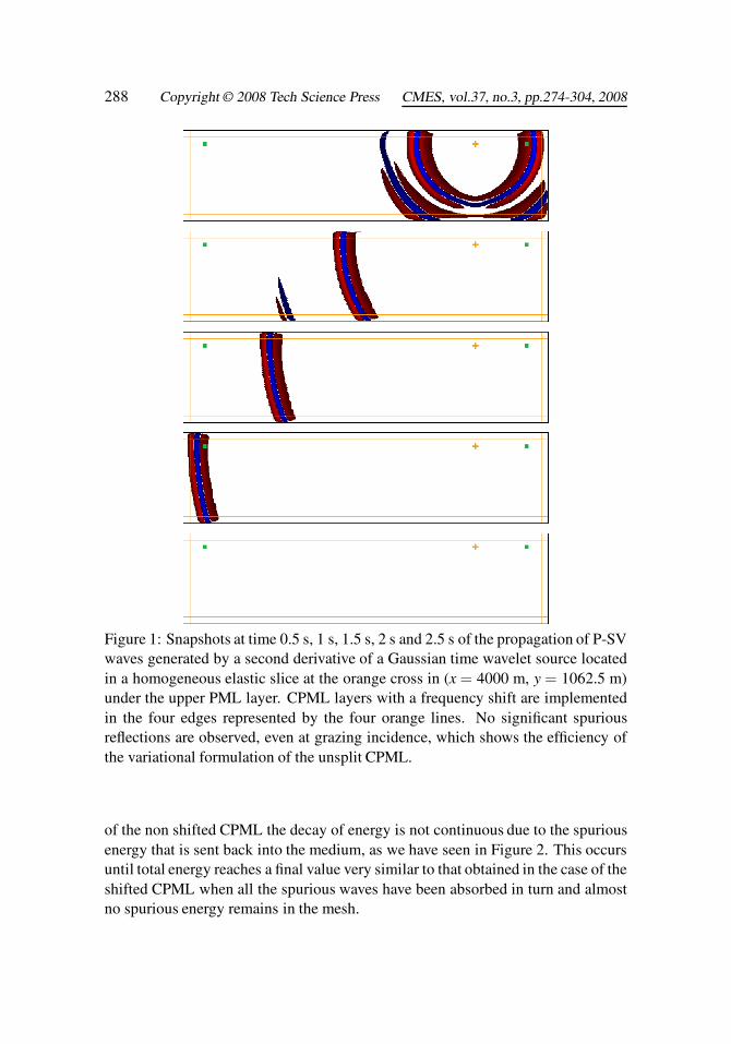
Figure 1: Snapshots at time 0.5 s, 1 s, 1.5 s, 2 s and 2.5 s of the propagation of P-SVwaves generated by a second derivative of a Gaussian time wavelet source locatedin a homogeneous elastic slice at the orange cross in (x = 4000 m, y = 1062.5 m)under the upper PML layer. CPML layers with a frequency shift are implementedin the four edges represented by the four orange lines. No significant spuriousreflections are observed, even at grazing incidence, which shows the efficiency ofthe variational formulation of the unsplit CPML.

of the non shifted CPML the decay of energy is not continuous due to the spuriousenergy that is sent back into the medium, as we have seen in Figure 2. This occursuntil total energy reaches a final value very similar to that obtained in the case of theshifted CPML when all the spurious waves have been absorbed in turn and almostno spurious energy remains in the mesh.


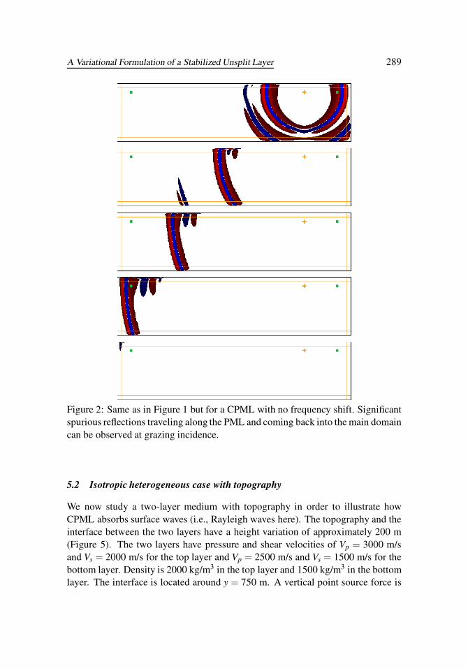
Figure 2: Same as in Figure 1 but for a CPML with no frequency shift. Significantspurious reflections traveling along the PML and coming back into the main domaincan be observed at grazing incidence.

5.2 Isotropic heterogeneous case with topography

We now study a two-layer medium with topography in order to illustrate howCPML absorbs surface waves (i.e., Rayleigh waves here). The topography and theinterface between the two layers have a height variation of approximately 200 m(Figure 5). The two layers have pressure and shear velocities of Vp = 3000 m/sand Vs = 2000 m/s for the top layer and Vp = 2500 m/s and Vs = 1500 m/s for thebottom layer. Density is 2000 kg/m3 in the top layer and 1500 kg/m3 in the bottomlayer. The interface is located around y = 750 m. A vertical point source force is


-0.002

-0.0015

-0.001

-0.0005

0

0.0005

0.001

0.0015

1 1.2 1.4 1.6 1.8 2 2.2 2.4 2.6 2.8

Am

plitu

de (

m)

Time (s)

CPML Reference solution

-0.002

-0.0015

-0.001

-0.0005

0

0.0005

0.001

0.0015

1 1.2 1.4 1.6 1.8 2 2.2 2.4 2.6 2.8

Am

plitu

de (

m)

Time (s)

CPML alpha=0Reference solution

-0.005

-0.004

-0.003

-0.002

-0.001

0

0.001

0.002

0.003

0 0.2 0.4 0.6 0.8 1 1.2 1.4

Am

plitu

de (

m)

Time (s)

CPML Reference solution

-0.005

-0.004

-0.003

-0.002

-0.001

0

0.001

0.002

0.003

0 0.2 0.4 0.6 0.8 1 1.2 1.4

Am

plitu

de (

m)

Time (s)

CPML alpha=0Reference solution

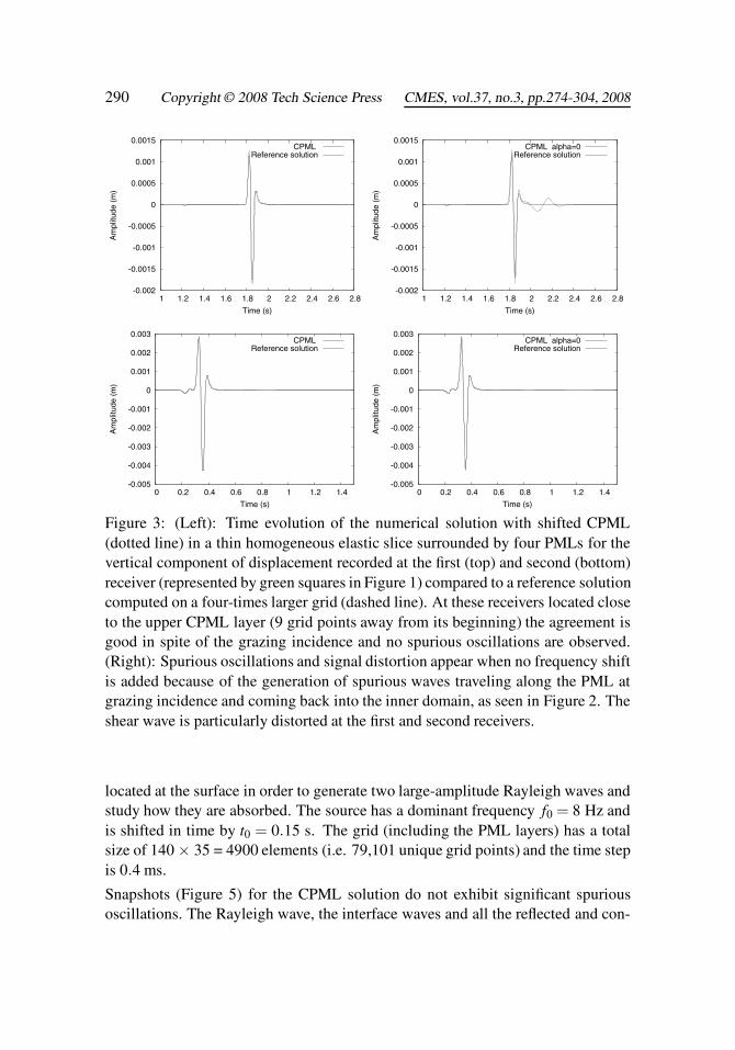
Figure 3: (Left): Time evolution of the numerical solution with shifted CPML(dotted line) in a thin homogeneous elastic slice surrounded by four PMLs for thevertical component of displacement recorded at the first (top) and second (bottom)receiver (represented by green squares in Figure 1) compared to a reference solutioncomputed on a four-times larger grid (dashed line). At these receivers located closeto the upper CPML layer (9 grid points away from its beginning) the agreement isgood in spite of the grazing incidence and no spurious oscillations are observed.(Right): Spurious oscillations and signal distortion appear when no frequency shiftis added because of the generation of spurious waves traveling along the PML atgrazing incidence and coming back into the inner domain, as seen in Figure 2. Theshear wave is particularly distorted at the first and second receivers.

located at the surface in order to generate two large-amplitude Rayleigh waves andstudy how they are absorbed. The source has a dominant frequency f0 = 8 Hz andis shifted in time by t0 = 0.15 s. The grid (including the PML layers) has a totalsize of 140 × 35 = 4900 elements (i.e. 79,101 unique grid points) and the time stepis 0.4 ms.

Snapshots (Figure 5) for the CPML solution do not exhibit significant spuriousoscillations. The Rayleigh wave, the interface waves and all the reflected and con-


1e-10

1e-08

1e-06

0.0001

0.01

1

100

10000

1 2 3 4 5 6 7 8 9 10

Ene

rgy

(J)

Time (s)

CPML n=2 m=1CPML n=2 alpha=0

1e-12

1e-10

1e-08

1e-06

0.0001

0.01

1

100

10000

10 20 30 40 50 60 70 80 90 100

Ene

rgy

(J)

Time (s)

CPML n=2 m=1CPML n=2 alpha=0

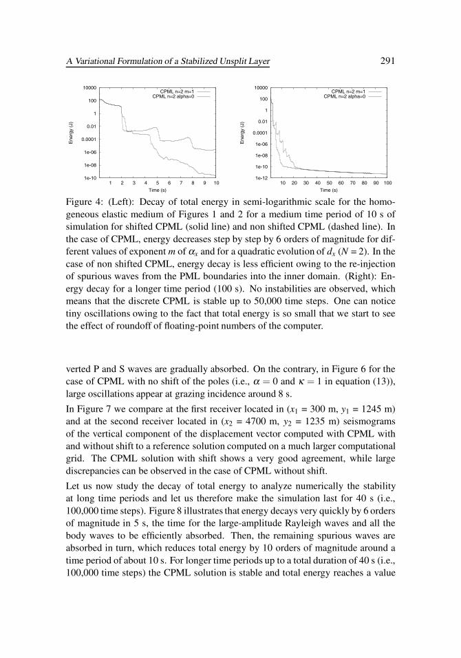
Figure 4: (Left): Decay of total energy in semi-logarithmic scale for the homo-geneous elastic medium of Figures 1 and 2 for a medium time period of 10 s ofsimulation for shifted CPML (solid line) and non shifted CPML (dashed line). Inthe case of CPML, energy decreases step by step by 6 orders of magnitude for dif-ferent values of exponent m of αx and for a quadratic evolution of dx (N = 2). In thecase of non shifted CPML, energy decay is less efficient owing to the re-injectionof spurious waves from the PML boundaries into the inner domain. (Right): En-ergy decay for a longer time period (100 s). No instabilities are observed, whichmeans that the discrete CPML is stable up to 50,000 time steps. One can noticetiny oscillations owing to the fact that total energy is so small that we start to seethe effect of roundoff of floating-point numbers of the computer.

verted P and S waves are gradually absorbed. On the contrary, in Figure 6 for thecase of CPML with no shift of the poles (i.e., α = 0 and κ = 1 in equation (13)),large oscillations appear at grazing incidence around 8 s.

In Figure 7 we compare at the first receiver located in (x1 = 300 m, y1 = 1245 m)and at the second receiver located in (x2 = 4700 m, y2 = 1235 m) seismogramsof the vertical component of the displacement vector computed with CPML withand without shift to a reference solution computed on a much larger computationalgrid. The CPML solution with shift shows a very good agreement, while largediscrepancies can be observed in the case of CPML without shift.

Let us now study the decay of total energy to analyze numerically the stabilityat long time periods and let us therefore make the simulation last for 40 s (i.e.,100,000 time steps). Figure 8 illustrates that energy decays very quickly by 6 ordersof magnitude in 5 s, the time for the large-amplitude Rayleigh waves and all thebody waves to be efficiently absorbed. Then, the remaining spurious waves areabsorbed in turn, which reduces total energy by 10 orders of magnitude around atime period of about 10 s. For longer time periods up to a total duration of 40 s (i.e.,100,000 time steps) the CPML solution is stable and total energy reaches a value


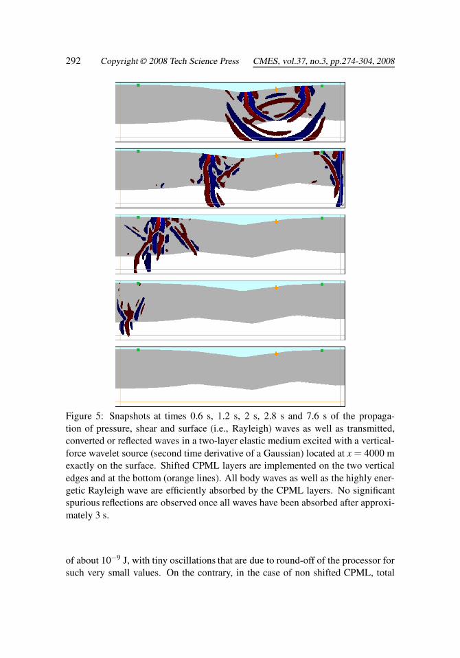
Figure 5: Snapshots at times 0.6 s, 1.2 s, 2 s, 2.8 s and 7.6 s of the propaga-tion of pressure, shear and surface (i.e., Rayleigh) waves as well as transmitted,converted or reflected waves in a two-layer elastic medium excited with a vertical-force wavelet source (second time derivative of a Gaussian) located at x = 4000 mexactly on the surface. Shifted CPML layers are implemented on the two verticaledges and at the bottom (orange lines). All body waves as well as the highly ener-getic Rayleigh wave are efficiently absorbed by the CPML layers. No significantspurious reflections are observed once all waves have been absorbed after approxi-mately 3 s.

of about 10−9 J, with tiny oscillations that are due to round-off of the processor forsuch very small values. On the contrary, in the case of non shifted CPML, total


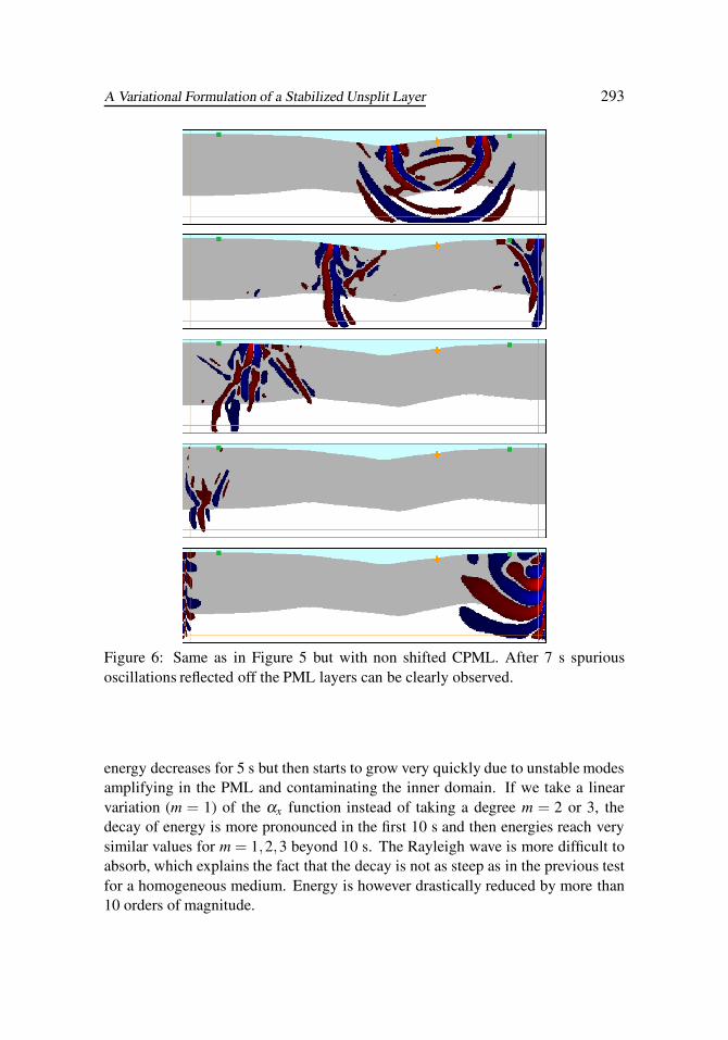
Figure 6: Same as in Figure 5 but with non shifted CPML. After 7 s spuriousoscillations reflected off the PML layers can be clearly observed.

energy decreases for 5 s but then starts to grow very quickly due to unstable modesamplifying in the PML and contaminating the inner domain. If we take a linearvariation (m = 1) of the αx function instead of taking a degree m = 2 or 3, thedecay of energy is more pronounced in the first 10 s and then energies reach verysimilar values for m = 1,2,3 beyond 10 s. The Rayleigh wave is more difficult toabsorb, which explains the fact that the decay is not as steep as in the previous testfor a homogeneous medium. Energy is however drastically reduced by more than10 orders of magnitude.


-0.05

-0.04

-0.03

-0.02

-0.01

0

0.01

0.02

0.03

0.04

0.05

1 1.5 2 2.5 3 3.5

Am

plitu

de (

m)

Time (s)

CPML n=3 m=3Vy CPML n=2 m=2Vy CPML n=2 m=1

Vy referenceCPML n=2 alpha=0

-0.05

-0.04

-0.03

-0.02

-0.01

0

0.01

0.02

0.03

0.04

0.05

1 2 3 4 5 6 7 8 9 10

Am

plitu

de (

m)

Time (s)

CPML n=2 alpha=0Vy reference

-0.05

-0.04

-0.03

-0.02

-0.01

0

0.01

0.02

0.03

0.04

0.05

0 0.5 1 1.5 2

Am

plitu

de (

m)

Time (s)

CPML n=3 m=3Vy CPML n=2 m=2Vy CPML n=2 m=1

Vy referenceCPML n=2 alpha=0

-0.2

-0.15

-0.1

-0.05

0

0.05

0.1

0.15

1 2 3 4 5 6 7 8 9 10

Am

plitu

de (

m)

Time (s)

CPML n=2 alpha=0Vy reference

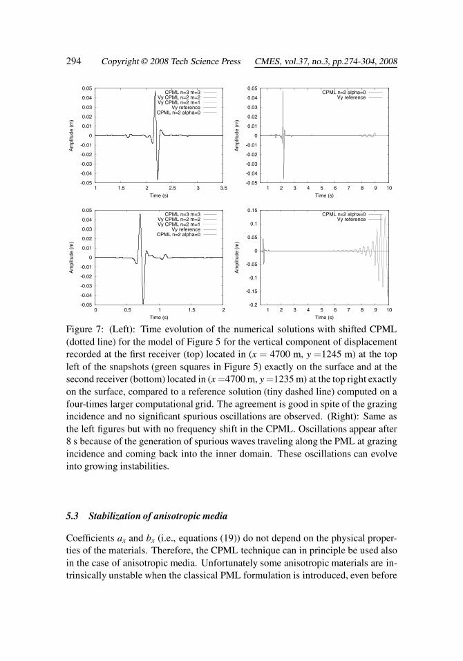
Figure 7: (Left): Time evolution of the numerical solutions with shifted CPML(dotted line) for the model of Figure 5 for the vertical component of displacementrecorded at the first receiver (top) located in (x = 4700 m, y =1245 m) at the topleft of the snapshots (green squares in Figure 5) exactly on the surface and at thesecond receiver (bottom) located in (x =4700 m, y =1235 m) at the top right exactlyon the surface, compared to a reference solution (tiny dashed line) computed on afour-times larger computational grid. The agreement is good in spite of the grazingincidence and no significant spurious oscillations are observed. (Right): Same asthe left figures but with no frequency shift in the CPML. Oscillations appear after8 s because of the generation of spurious waves traveling along the PML at grazingincidence and coming back into the inner domain. These oscillations can evolveinto growing instabilities.

5.3 Stabilization of anisotropic media

Coefficients ax and bx (i.e., equations (19)) do not depend on the physical proper-ties of the materials. Therefore, the CPML technique can in principle be used alsoin the case of anisotropic media. Unfortunately some anisotropic materials are in-trinsically unstable when the classical PML formulation is introduced, even before


1e-10

1e-08

1e-06

0.0001

0.01

1

100

10000

1e+06

5 10 15 20 25 30 35 40

Ene

rgy

(J)

Time (s)

CPML n=2 m=3CPML n=2 m=2CPML n=2 m=1

CPML n=2 alpha=0

Figure 8: Total energy decay in semi-logarithmic scale for the heterogeneous elas-tic medium of Figures 5 and 6 for a long time period of 70 s of simulation for shiftedCPML and non shifted CPML (α = 0). No instabilities are observed when a fre-quency shift is used, which means that the discrete CPML is stable up to 70,000time steps. It seems that a linear variation of αx (m = 1) and a quadratic polyno-mial (N=2) describing dx are reasonable values and provide better energy decay.All these cases finally lead to similar energies around 10−9 J beyond 20 s. After20 s one can notice tiny oscillations owing to the fact that total energy is so smallthat we start to see the effect of roundoff of floating-point numbers of the computer.In the case of non shifted CPML (α =0), energy starts to increase very quickly afterapproximately 5 s owing to growing instabilities that develop in the PML layers.

discretization by a numerical scheme (e.g., Bécache, Fauqueux, and Joly, 2003).But Meza-Fajardo and Papageorgiou (2008) have shown that modifications can beintroduced in the damping profiles to stabilize the discrete system. It is possible tointroduce corrections in the damping profiles dx by adding an extra damping pro-file in the orthogonal direction i.e. writing dx(x,y) = dx

x(x)+ dyx(y), dx

x(x) beingthe classical damping profile in the x direction inside the PML (as in the previoussections) and dy

x(y) = cx(x,y)dxx(x) the corrected damping profile in direction y.

cx(x,y) is generally a function varying between 0 and 1 inside the PML. The samecan be done for dy (see Figure 9). Meza-Fajardo and Papageorgiou (2008) usedthis correction for the split formulation of the PML conditions in a finite-differencecontext. Here we introduce it in our unsplit variational CPML technique with noextra cost in terms of memory storage.

Let us use strongly anisotropic materials inside the PML layers: an apatite crys-tal of stiffness coefficients in reduced Voigt notation c11 = 1.4×1011 N.m, c22 =


Figure 9: Definition of the corrected damping profiles in all the PML layers ofMeza-Fajardo and Papageorgiou (2008) that are used to stabilize the CPML formu-lation for anisotropic media.

Figure 10: Snapshots at times 20, 60, 100, 140 and 500 μs for an apatite crystalwithout a frequency shift when a corrected damping profiles are introduced. Noinstabilities are observed, while the same snapshots without correction shown inKomatitsch and Martin (2007) (Figure 10 of that article) show that the simulationwith no correction is unstable. Snapshots for a shifted CPML are very similar andtherefore not shown here.

1.67×1011 N.m, c12 = 6.6×1010 N.m, c33 = 6.63×1010 N.m, and density ρ =3200 kg/m3; or a zinc crystal (c11 = 1.65× 1011 N.m, c22 = 6.2× 1010 N.m,c12 = 5× 1010 N.m, c33 = 3.96× 1010 N.m, and density ρ = 7100 kg/m3). Asexplained by Bécache, Fauqueux, and Joly (2003) and demonstrated numericallyin Komatitsch and Martin (2007), these models are intrinsically unstable at high


1e-10

1e-05

1

100000

1e+10

1e+15

1e+20

1e+25

1e+30

1e+35

1e+40

0 0.001 0.002 0.003 0.004 0.005 0.006 0.007 0.008

Ene

rgy

(J)

Time (s)

CPML no shift, no correction CPML with shift, no correction

1e-12

1e-10

1e-08

1e-06

0.0001

0.01

1

100

10000

1e+06

1e+08

0 0.001 0.002 0.003 0.004 0.005 0.006 0.007 0.008

Ene

rgy

(J)

Time (s)

No shift, correction d_yx=0.03With shift, correction d_yx=0.03

No shift, correction d_yx=0.1

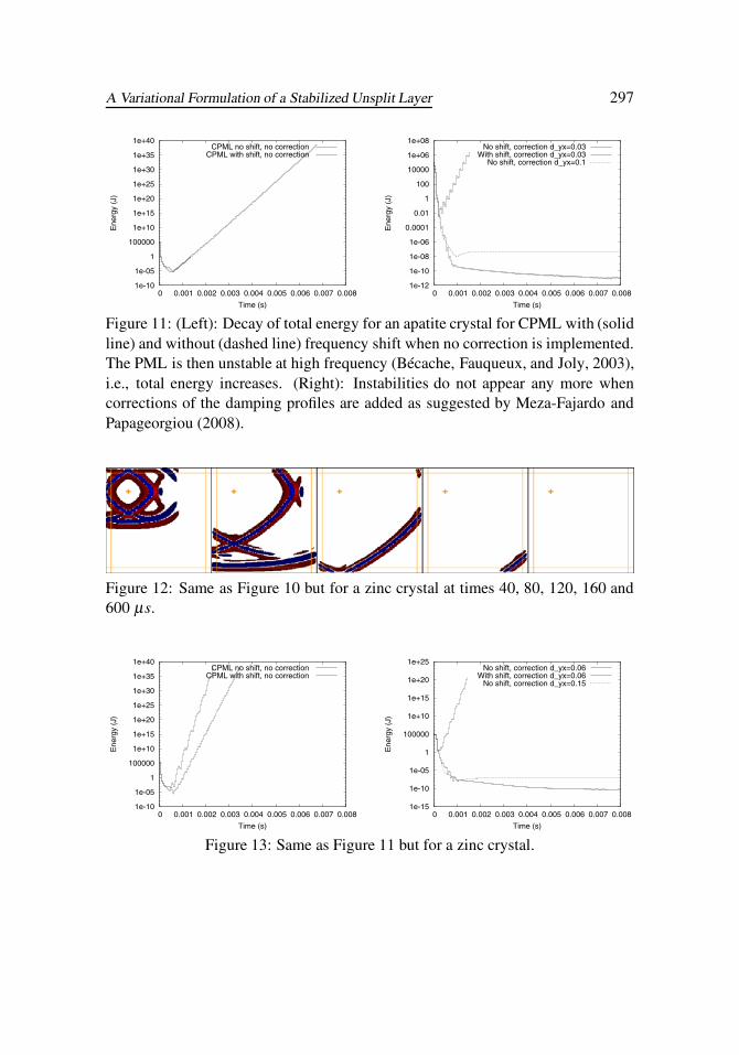
Figure 11: (Left): Decay of total energy for an apatite crystal for CPML with (solidline) and without (dashed line) frequency shift when no correction is implemented.The PML is then unstable at high frequency (Bécache, Fauqueux, and Joly, 2003),i.e., total energy increases. (Right): Instabilities do not appear any more whencorrections of the damping profiles are added as suggested by Meza-Fajardo andPapageorgiou (2008).

Figure 12: Same as Figure 10 but for a zinc crystal at times 40, 80, 120, 160 and600 μs.

1e-10

1e-05

1

100000

1e+10

1e+15

1e+20

1e+25

1e+30

1e+35

1e+40

0 0.001 0.002 0.003 0.004 0.005 0.006 0.007 0.008

Ene

rgy

(J)

Time (s)

CPML no shift, no correction CPML with shift, no correction

1e-15

1e-10

1e-05

1

100000

1e+10

1e+15

1e+20

1e+25

0 0.001 0.002 0.003 0.004 0.005 0.006 0.007 0.008

Ene

rgy

(J)

Time (s)

No shift, correction d_yx=0.06With shift, correction d_yx=0.06

No shift, correction d_yx=0.15

Figure 13: Same as Figure 11 but for a zinc crystal.


frequency because at least one of the following conditions is violated:

((c12 +c33)2 −c11(c22−c33)) ((c12 +c33)2 +c33(c22−c33))≤ 0

(c12 +2c33)2 −c11 c22 ≤ 0

(c12 +c33)2−c11 c22 −c233 ≤ 0 (32)

Let us therefore use a source with high frequency content: the second time deriva-tive of a Gaussian with a dominant frequency of 100 Hz. Indeed, in the case of bothapatite and zinc crystals, the total energy quickly blows up when no corrections ofthe damping functions are introduced (Figures 11 and 13). This means that the sim-ulations become unstable at time periods beyond 0.001 s independently of using afrequency shift in CPML or not. However, using the correction of Meza-Fajardoand Papageorgiou (2008) it is possible to enforce the high-frequency stability con-ditions for the quasi-shear wave of equation (32) by using a suitable value of thecorrection factor cx. In Figures 10 (apatite) and 12 (zinc), we show snapshots atdifferent times (short, medium and long time periods) of wave propagation for thetwo fully anisotropic materials under study when the corrections of damping pro-files are introduced. The simulations remain stable for long time periods even forsuch a source located in a corner of the computational domain and close to the baseof the PML, which is a difficult case because a very significant part of the energyof the source is quickly sent into the PML layers. Here, cx = cy = 0.03 (apatite) orcx = cy = 0.06 (zinc) allow for a stabilization of CPML when a frequency shift isused, while higher values of 0.1 for apatite and 0.15 for zinc are needed to stabilizeit when no frequency shift is used (Figures 11 and 13). Total energy diverges whenno correction is used while it decays by around 12 orders of magnitude until reach-ing values around 10−10 J or 10−11 J at long time periods of 0.008 s (200,000 timesteps) when corrections are used. If high damping corrections are added in the nonshifted case, total energy decay is enforced at the expense of a small distortion ofthe wave patterns near the boundaries (not shown here).

6 Conclusions and future work

We have extended the unsplit convolutional perfectly matched layer (CPML) tech-nique to the variational formulation of the seismic wave equation discretized basedupon a spectral-element method. We have been able to absorb not only pressureand shear waves in a homogeneous medium but also surface waves in a heteroge-neous medium in the presence of topography. The introduction of corrections in thedamping profiles along the different coordinate axes has stabilized the numericaltechnique at high frequency in the case of anisotropic media that are intrinsicallyunstable when the classical PML is used. The memory storage of the CPML is


smaller by about 35% compared to the classical split PML (if only split variablesv j

i are stored in memory) or to optimized split PMLs such as the GFPML technique(Festa and Vilotte, 2005), and by about 48% if split variables and total fields vi areboth stored in memory. In 3D the CPML technique reduces the memory storageby about 44% compared to the classical split PML or to the GFPML if only splitvariables are stored in memory, and by about 53% if split variables and total fieldsvi are both stored in memory. In the case of an implementation of the spectral-element method on a parallel computer (e.g., Martin, Komatitsch, Blitz, and LeGoff, 2008), efforts will need to be made in order to balance the number of calcu-lations inside and outside the PML because the number of computations is higherinside the PMLs than outside.

Acknowledgement: The authors thank Julien Diaz for fruitful discussions on thevariational formulation.

References

Abarbanel, S.; Gottlieb, D.; Hesthaven, J. S. (2002): Long-time behavior ofthe perfectly matched layer equations in computational electromagnetics. J. Sc.Comp., vol. 17, pp. 405–422.

Abreu, A. I.; Mansur, W. J.; Soares-Jr, D.; Carrer, J. A. M. (2008): Numericalcomputation of space derivatives by the complex-variable-differentiation methodin the convolution quadrature method based BEM formulation. CMES: ComputerModeling in Engineering & Sciences, vol. 30, no. 3, pp. 123–132.

Alterman, Z.; Karal, F. C. (1968): Propagation of elastic waves in layered mediaby finite difference methods. Bull. Seismol. Soc. Am., vol. 58, pp. 367–398.

Bao, H.; Bielak, J.; Ghattas, O.; Kallivokas, L. F.; O’Hallaron, D. R.;Shewchuk, J. R.; Xu, J. (1998): Large-scale simulation of elastic wave prop-agation in heterogeneous media on parallel computers. Comput. Methods Appl.Mech. Engrg., vol. 152, pp. 85–102.

Basu, U. (2009): Explicit finite element perfectly matched layer for transientthree-dimensional elastic waves. Int. J. Numer. Meth. Engng., vol. 77, pp. 151–176.

Basu, U.; Chopra, A. K. (2004): Perfectly matched layers for transient elas-todynamics of unbounded domains. Int. J. Numer. Meth. Engng., vol. 59, pp.1039–1074.


Bécache, E.; Fauqueux, S.; Joly, P. (2003): Stability of perfectly matched layers,group velocities and anisotropic waves. J. Comput. Phys., vol. 188, no. 2, pp.399–433.

Bécache, E.; Joly, P. (2002): On the analysis of Bérenger’s perfectly matchedlayers for Maxwell’s equations. M2AN, vol. 36, no. 1, pp. 87–120.

Bérenger, J. P. (1994): A Perfectly Matched Layer for the absorption of electro-magnetic waves. J. Comput. Phys., vol. 114, pp. 185–200.

Bérenger, J. P. (2002): Application of the CFS PML to the absorption of evanes-cent waves in waveguides. IEEE Microwave and Wireless Components Letters,vol. 12, no. 6, pp. 218–220.

Bérenger, J. P. (2002): Numerical reflection from FDTD-PMLs: A comparisonof the split PML with the unsplit and CFS PMLs. IEEE Transactions on Antennasand Propagation, vol. 50, no. 3, pp. 258–265.

Carcione, J. M. (1994): The wave equation in generalized coordinates. Geo-physics, vol. 59, pp. 1911–1919.

Cerjan, C.; Kosloff, D.; Kosloff, R.; Reshef, M. (1985): A nonreflecting bound-ary condition for discrete acoustic and elastic wave equation. Geophysics, vol. 50,pp. 705–708.

Chew, W. C.; Liu, Q. (1996): Perfectly Matched Layers for elastodynamics: anew absorbing boundary condition. J. Comput. Acoust., vol. 4, no. 4, pp. 341–359.

Chew, W. C.; Weedon, W. H. (1994): A 3-D perfectly matched medium frommodified Maxwell’s equations with stretched coordinates. Microwave Opt. Tech-nol. Lett., vol. 7, no. 13, pp. 599–604.

Clayton, R.; Engquist, B. (1977): Absorbing boundary conditions for acousticand elastic wave equations. Bull. Seismol. Soc. Am., vol. 67, pp. 1529–1540.

Cohen, G.; Fauqueux, S. (2005): Mixed spectral finite elements for the linearelasticity system in unbounded domains. SIAM Journal on Scientific Computing,vol. 26, no. 3, pp. 864–884.

Collino, F.; Monk, P. (1998): The Perfectly Matched Layer in curvilinear coordi-nates. SIAM J. Sci. Comput., vol. 19, no. 6, pp. 2061–2090.

Collino, F.; Tsogka, C. (2001): Application of the PML absorbing layer model tothe linear elastodynamic problem in anisotropic heterogeneous media. Geophysics,vol. 66, no. 1, pp. 294–307.


Dong, L.; She, D.; Guan, L.; Ma, Z. (2005): An eigenvalue decompositionmethod to construct absorbing boundary conditions for acoustic and elastic waveequations. J. Geophys. Eng., vol. 2, pp. 192–198.

Drossaert, F. H.; Giannopoulos, A. (2007): A nonsplit complex frequency-shifted PML based on recursive integration for FDTD modeling of elastic waves.Geophysics, vol. 72, no. 2, pp. T9–T17.

Dumbser, M.; Käser, M. (2006): An arbitrary high-order discontinu-ous Galerkin method for elastic waves on unstructured meshes-II. The three-dimensional isotropic case. Geophys. J. Int., vol. 167, no. 1, pp. 319–336.

Engquist, B.; Majda, A. (1977): Absorbing boundary conditions for the numeri-cal simulation of waves. Math. Comp., vol. 31, pp. 629–651.

Fauqueux, S. (2003): Eléments finis mixtes spectraux et couches absorbantesparfaitement adaptées pour la propagation d’ondes élastiques en régime transi-toire. PhD thesis, Université Paris-Dauphine, France, 2003.

Festa, G.; Delavaud, E.; Vilotte, J. P. (2005): Interaction between surface wavesand absorbing boundaries for wave propagation in geological basins: 2D numericalsimulations. Geophys. Res. Lett., vol. 32, no. 20, pp. L20306.

Festa, G.; Vilotte, J. P. (2005): The Newmark scheme as velocity-stress time-staggering: an efficient PML implementation for spectral-element simulations ofelastodynamics. Geophys. J. Int., vol. 161, pp. 789–812.

Gedney, S. D. (1998): The Perfectly Matched Layer absorbing medium.In Taflove, A.(Ed): Advances in Computational Electrodynamics: the Finite-Difference Time-Domain method, chapter 5, pp. 263–343. Artech House, Boston.

Gedney, S. D.; Zhao, B. (2009): An Auxiliary Differential Equation Formulationfor the Complex-Frequency Shifted PML. IEEE Transactions on Antennas andPropagation. Submitted.

Givoli, D. (1991): Non-reflecting boundary conditions: review article. J. Comput.Phys., vol. 94, pp. 1–29.

Givoli, D. (2004): High-order local non-reflecting boundary conditions: A review.Wave Motion, vol. 39, pp. 319–326.

Givoli, D. (2008): Computational absorbing boundaries. In Marburg, S.; Nolte,B.(Eds): Computational Acoustics Noise Propagation in Fluids, volume 5, pp.145–166. Springer-Verlag, Berlin, Germany.


Grote, M. J. (2000): Nonreflecting boundary conditions for elastodynamics scat-tering. J. Comput. Phys., vol. 161, pp. 331–353.

Guddati, M. N.; Lim, K. W. (2006): Continued fraction absorbing boundaryconditions for convex polygonal domains. Int. J. Numer. Meth. Engng., vol. 66,no. 6, pp. 949–977.

Hagstrom, T. (1999): Radiation boundary conditions for the numerical simulationof waves. Acta Numerica, vol. 8, pp. 47–106.

Hagstrom, T.; Hariharan, S. I. (1998): A formulation of asymptotic and exactboundary conditions using local operators. Appl. Num. Math., vol. 27, pp. 403–416.

Higdon, R. L. (1991): Absorbing boundary conditions for elastic waves. Geo-physics, vol. 56, pp. 231–241.

Hughes, T. J. R. (1987): The finite element method, linear static and dynamicfinite element analysis. Prentice-Hall International, Englewood Cliffs, New Jersey,USA.

Kawase, H. (1988): Time-domain response of a semi-circular canyon for inci-dent SV, P and Rayleigh waves calculated by the discrete wavenumber boundaryelement method. Bull. Seismol. Soc. Am., vol. 78, pp. 1415–1437.

Komatitsch, D.; Martin, R. (2007): An unsplit convolutional Perfectly MatchedLayer improved at grazing incidence for the seismic wave equation. Geophysics,vol. 72, no. 5, pp. SM155–SM167.

Komatitsch, D.; Martin, R.; Tromp, J.; Taylor, M. A.; Wingate, B. A. (2001):Wave propagation in 2-D elastic media using a spectral element method with trian-gles and quadrangles. J. Comput. Acoust., vol. 9, no. 2, pp. 703–718.

Komatitsch, D.; Tromp, J. (1999): Introduction to the spectral-element methodfor 3-D seismic wave propagation. Geophys. J. Int., vol. 139, no. 3, pp. 806–822.

Komatitsch, D.; Tromp, J. (2003): A Perfectly Matched Layer absorbing bound-ary condition for the second-order seismic wave equation. Geophys. J. Int., vol.154, no. 1, pp. 146–153.

Komatitsch, D.; Vilotte, J. P. (1998): The spectral-element method: an efficienttool to simulate the seismic response of 2D and 3D geological structures. Bull.Seismol. Soc. Am., vol. 88, no. 2, pp. 368–392.


Kuzuoglu, M.; Mittra, R. (1996): Frequency dependence of the constitutiveparameters of causal perfectly matched anisotropic absorbers. IEEE Microwaveand Guided Wave Letters, vol. 6, no. 12, pp. 447–449.

Lu, Y. Y.; Zhu, J. (2007): Perfectly matched layer for acoustic waveguide mod-eling - Benchmark calculations and perturbation analysis. CMES: Computer Mod-eling in Engineering & Sciences, vol. 22, no. 3, pp. 235–248.

Luebbers, R. J.; Hunsberger, F. (1992): FDTD for Nth-order dispersive media.IEEE Transactions on Antennas and Propagation, vol. 40, no. 11, pp. 1297–1301.

Lysmer, J.; Drake, L. A. (1972): A finite element method for seismology. InMethods in Computational Physics, volume 11. Academic Press, New York, USA.

Ma, S.; Liu, P. (2006): Modeling of the perfectly matched layer absorbing bound-aries and intrinsic attenuation in explicit finite-element methods. Bull. Seismol.Soc. Am., vol. 96, no. 5, pp. 1779–1794.

Madariaga, R. (1976): Dynamics of an expanding circular fault. Bull. Seismol.Soc. Am., vol. 66, no. 3, pp. 639–666.

Martin, R.; Komatitsch, D.; Blitz, C.; Le Goff, N. (2008): Simulation of seismicwave propagation in an asteroid based upon an unstructured MPI spectral-elementmethod: blocking and non-blocking communication strategies. Lecture Notes inComputer Science, vol. 5336, pp. 350–363.

Martin, R.; Komatitsch, D.; Ezziani, A. (2008): An unsplit convolutional Per-fectly Matched Layer improved at grazing incidence for seismic wave equation inporoelastic media. Geophysics, vol. 73, no. 4, pp. T51–T61.

Meza-Fajardo, K. C.; Papageorgiou, A. S. (2008): A nonconvolutional, split-field, perfectly matched layer for wave propagation in isotropic and anisotropicelastic media; stability analysis. Bull. Seismol. Soc. Am., vol. 98, no. 4, pp. 1811–1836.

Moczo, P.; Kristek, J.; Bystrický, E. (2001): Efficiency and optimization of the3-D finite-difference modeling of seismic ground motion. J. Comput. Acoust., vol.9, no. 2, pp. 593–609.

Nissen-Meyer, T.; Fournier, A.; Dahlen, F. A. (2008): A 2-D spectral-elementmethod for computing spherical-earth seismograms - II. Waves in solid-fluid me-dia. Geophys. J. Int., vol. 174, pp. 873–888.


Peng, C. B.; Töksoz, M. N. (1995): An optimal absorbing boundary conditionfor elastic wave modeling. Geophysics, vol. 60, pp. 296–301.

Roden, J. A.; Gedney, S. D. (2000): Convolution PML (CPML): An efficientFDTD implementation of the CFS-PML for arbitrary media. Microwave and Op-tical Technology Letters, vol. 27, no. 5, pp. 334–339.

Rodríguez-Castellanos, A.; Sánchez-Sesma, F.; Luzón, F.; Martin, R. (2006):Multiple scattering of elastic waves by subsurface fractures and cavities. Bull.Seismol. Soc. Am., vol. 96, no. 4A, pp. 1359–1374.

Sánchez-Sesma, F. J.; Campillo, M. (1991): Diffraction of P, SV and Rayleighwaves by topographic features: a boundary integral formulation. Bull. Seismol.Soc. Am., vol. 81, pp. 2234–2253.

Simo, J. C.; Tarnow, N.; Wong, K. K. (1992): Exact energy-momentum conserv-ing algorithms and symplectic schemes for nonlinear dynamics. Comput. MethodsAppl. Mech. Engrg., vol. 100, pp. 63–116.

Soares-Jr, D.; Mansur, W. J.; Lima, D. L. (2007): An explicit multi-level time-step algorithm to model the propagation of interacting acoustic-elastic waves usingfinite-element/finite-difference coupled procedures. CMES: Computer Modelingin Engineering & Sciences, vol. 17, no. 1, pp. 19–34.

Sochacki, J.; Kubichek, R.; George, J.; Fletcher, W. R.; Smithson, S. (1987):Absorbing boundary conditions and surface waves. Geophysics, vol. 52, no. 1, pp.60–71.

Stacey, R. (1988): Improved transparent boundary formulations for the elasticwave equation. Bull. Seismol. Soc. Am., vol. 78, no. 6, pp. 2089–2097.

Tessmer, E.; Kosloff, D. (1994): 3-D elastic modeling with surface topographyby a Chebyshev spectral method. Geophysics, vol. 59, no. 3, pp. 464–473.

Virieux, J. (1986): P-SV wave propagation in heterogeneous media: velocity-stress finite-difference method. Geophysics, vol. 51, pp. 889–901.

Zeng, Y. Q.; He, J. Q.; Liu, Q. H. (2001): The application of the perfectlymatched layer in numerical modeling of wave propagation in poroelastic media.Geophysics, vol. 66, no. 4, pp. 1258–1266.

A Variational Formulation of a Stabilized Unsplit Convolutional Perfectly Matched Layer for The...

Documents

Transcript of A Variational Formulation of a Stabilized Unsplit Convolutional Perfectly Matched Layer for The...