arX

iv:1

806.

0071

2v1

[cs

.CV

] 2

Jun

201

8

An Interpretable Deep Hierarchical Semantic Convolutional Neural

Network for Lung Nodule Malignancy Classification

Shiwen Shena,b, Simon X. Hana,b, Denise R. Aberlea,b, Alex A.T. Buib, Willliam Hsub,∗

aDepartment of Bioengineering, University of California, Los Angeles, CA, USAbMedical Imaging & Informatics Group, Department of Radiological Sciences, University of California, Los

Angeles, CA, USA

Abstract

While deep learning methods are increasingly being applied to tasks such as computer-aideddiagnosis, these models are difficult to interpret, do not incorporate prior domain knowledge,and are often considered as a “black-box.” The lack of model interpretability hinders themfrom being fully understood by target users such as radiologists. In this paper, we presenta novel interpretable deep hierarchical semantic convolutional neural network (HSCNN) topredict whether a given pulmonary nodule observed on a computed tomography (CT) scanis malignant. Our network provides two levels of output: 1) low-level radiologist semanticfeatures; and 2) a high-level malignancy prediction score. The low-level semantic outputsquantify the diagnostic features used by radiologists and serve to explain how the model in-terprets the images in an expert-driven manner. The information from these low-level tasks,along with the representations learned by the convolutional layers, are then combined andused to infer the high-level task of predicting nodule malignancy. This unified architecture istrained by optimizing a global loss function including both low- and high-level tasks, therebylearning all the parameters within a joint framework. Our experimental results using theLung Image Database Consortium (LIDC) show that the proposed method not only producesinterpretable lung cancer predictions but also achieves significantly better results comparedto common 3D CNN approaches.

Keywords: Lung nodule classification, lung cancer diagnosis, Computed tomography, deeplearning, convolutional neural networks, model interpretability

1. Introduction and Background

Lung cancer is the leading cause of cancer mortality worldwide [1, 2]. Computed to-mography (CT) imaging is widely used to detect pulmonary nodules and forms the basisfor diagnosing lung cancer. The landmark National Lung Screening Trial (NLST) [3] in theUnited States demonstrated a 20% lung cancer mortality reduction in high-risk subjects who

∗Medical Imaging & Informatics, 924 Westwood Boulevard, Suite 420, Los Angeles, CA 90024, USA.Email addresses: shiwenshen@engineering.ucla.edu (Shiwen Shen), simon.x.han@ucla.edu (Simon

X. Han), daberle@mednet.ucla.edu (Denise R. Aberle), buia@mii.ucla.edu (Alex A.T. Bui),whsu@mednet.ucla.edu (Willliam Hsu)

Preprint submitted to Expert Systems with Applications June 5, 2018

underwent screening using low-dose CT (relative to using plain chest radiography). Basedon the findings of the NLST, the United States Preventative Services Task Force (USPSTF)went on to recommend low-dose CT lung cancer screening for current and former smokersaged 55-80 with a smoking history of at least 30 pack-years, or former smokers having quitwithin the past 15 years [4]. However, the potential consequences of implementing lungcancer screening is an increase in false positive screens that result in unnecessary medical,economic, and psychological costs. Indeed, some studies indicate that the false positive ratefor low-dose CT is upwards of 20%; less experienced radiologists have highly variable de-tection rates, particularly in subtle cases, as interpretation heavily relies on past experience[5]. Figure 1 shows examples of malignant and benign nodules, helping to illustrate thechallenges of differentiating between the two groups.

Figure 1: Illustrations of malignant and benign nodules: R1 are malignant nodules; R2 are benign nodules.

In response, computer-aided diagnosis (CADx) systems [6, 7, 8, 9, 10, 11] have been ex-plored to assist radiologists in the interpretation process; these help to separate malignantfrom benign nodules and show promise in increasing the positive predictive value and re-ducing the false positive rates in characterizing small nodules [11]. Broadly, a contemporarylung nodule CADx system comprises three components: 1) nodule segmentation; 2) featureextraction from nodule candidates; and 3) classification of the candidate as benign or ma-lignant based on its extracted features. Segmentation of the lung nodule is the first stepto identify pertinent regions of interest (ROIs) so as to focus the ensuing analyses. In thesecond step, computed features such as texture, morphology, and gray-level statistics areextracted to characterize the nodule across various visual and spatial dimensions. Finally,using the computed features, the nodule candidates are categorized into benign or malignantby a classifier such as support vector machine, random forest, or gradient boosting tree. Forexample, Armato et al. [6] segmented the lung nodule using multilevel thresholding tech-niques; extracted morphological and gray-level features; and classified nodules as benign ormalignant using linear discriminant analysis. Zinovev et al. [12] employed both texture andintensity features using belief decision trees and a multi-label approach to perform lung nod-ule classification. Way et al. [13] segmented lung nodules using k-means clustering, combinednodule surface features together with texture and morphological features, and used linear

2

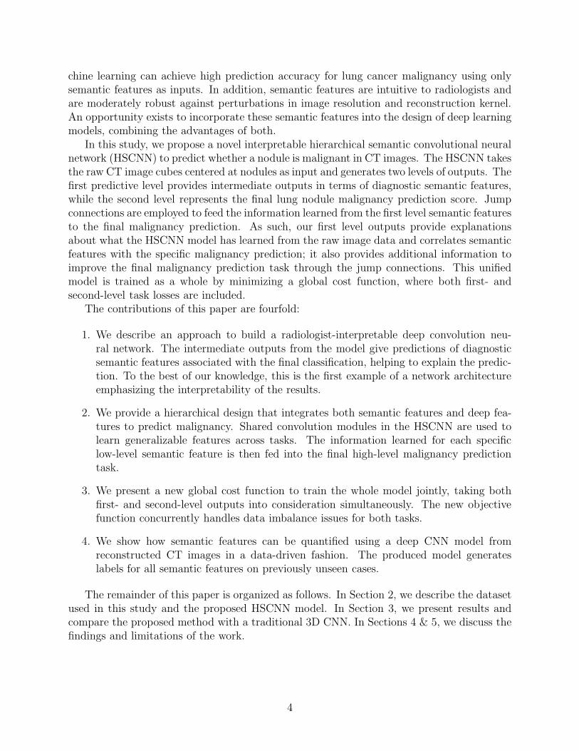
discriminant analysis to diagnose malignant lung cancers. Notably, the prevalent portion ofthese extracted features, such as volume and shape, are sensitive to the underlying variabilityarising from the lung nodule segmentation results. This variability may be caused by: 1)the challenges inherent in nodule delineation due to the range of nodule morphology andconnectivity complexity [14]; and 2) the variation posed by the computational segmentationmodels themselves in capturing quantitative characteristics [15, 16]. Thus, using segmentedregions may lead to inaccurate features that are subsequently used as inputs into downstreamclassifiers [15]. Another critical question raised by this type of CADx design is how to definethe “optimal” subset of features that can best encode characteristics of the lung nodule [17].The optimal feature set is dependent on the characteristics of the training dataset, and fea-ture selection and classification methods, which makes achieving comparable results usingdifferent datasets difficult.

To overcome these issues, deep learning methods [14, 15, 17, 18, 19], particularly convo-lutional neural networks (CNNs), have recently been used for lung nodule classification, withsome promising results. These deep learning models prove capable of adaptively learningimage representations in a fully data-driven way, taking raw image data as input withoutrelying on a priori nodule segmentation masks or handcrafted feature designs. For instance,Kumar et al. [18] first trained an unsupervised deep autoencoder to extract latent featuresfrom 2D CT patches. These extracted deep features were then used together with decisiontrees to predict lung cancer. Hua et al. [19] employed supervised techniques with a deep be-lief network and CNN to train models to classify lung nodules as benign or malignant. Theirmodels outperformed two baseline methods: using scale-invariant feature transform (SIFT)features and local binary patterns (LBP) [20]; and using fractal analysis [21]. Ciompi etal. [17] used pre-trained CNN models to classify candidates as peri-fissural nodules (PFNs)or non-PFNs. Deep features were extracted from the pre-trained model for three 2D imagepatches in axial, coronal, and sagittal views. An ensemble of the deep features and a bag offrequency features were then used to train supervised binary classifiers for the PFN classifi-cation task. Shen et. al. [14] designed a multi-scale CNN using 3D nodule patches at threescales to perform the lung cancer diagnosis task. This work is further extended in [15] byadding a multi-crop pooling strategy to improve model performance. Markedly, these citedworks use deep learning as a “black-box” and are not able to explain what representationshave been learned or why the model generates a given prediction. This low degree of inter-pretability arguably hinders domain experts, such as radiologists, from understanding howthe models work and ultimately impedes model adoption for clinical usage. As discussedin [22], improved interpretability is helpful to improve the radiologist-CAD interaction toallow radiologists to calibrate their trust in the CAD system. Moreover, human domainknowledge performs well across a wide range of observed nodule morphologies to differenti-ate benign from malignant nodules. Nonetheless, these domain knowledge are presently notincorporated into deep learning frameworks.

A number of radiologist-interpreted features derived from CT scans have been consid-ered influential when assessing the malignancy of a lung nodule [23, 24]. These featuresare referred to as diagnostic semantic features in this study. Examples of such semanticfeatures include nodule spiculation, lobulation, consistency (texture) and shape. Althoughqualitative in nature, studies have shown that these semantic features can be characterizednumerically using low-level image features [25]. Hancock et al. [26] demonstrated that ma-

3

chine learning can achieve high prediction accuracy for lung cancer malignancy using onlysemantic features as inputs. In addition, semantic features are intuitive to radiologists andare moderately robust against perturbations in image resolution and reconstruction kernel.An opportunity exists to incorporate these semantic features into the design of deep learningmodels, combining the advantages of both.

In this study, we propose a novel interpretable hierarchical semantic convolutional neuralnetwork (HSCNN) to predict whether a nodule is malignant in CT images. The HSCNN takesthe raw CT image cubes centered at nodules as input and generates two levels of outputs. Thefirst predictive level provides intermediate outputs in terms of diagnostic semantic features,while the second level represents the final lung nodule malignancy prediction score. Jumpconnections are employed to feed the information learned from the first level semantic featuresto the final malignancy prediction. As such, our first level outputs provide explanationsabout what the HSCNN model has learned from the raw image data and correlates semanticfeatures with the specific malignancy prediction; it also provides additional information toimprove the final malignancy prediction task through the jump connections. This unifiedmodel is trained as a whole by minimizing a global cost function, where both first- andsecond-level task losses are included.

The contributions of this paper are fourfold:

1. We describe an approach to build a radiologist-interpretable deep convolution neu-ral network. The intermediate outputs from the model give predictions of diagnosticsemantic features associated with the final classification, helping to explain the predic-tion. To the best of our knowledge, this is the first example of a network architectureemphasizing the interpretability of the results.

2. We provide a hierarchical design that integrates both semantic features and deep fea-tures to predict malignancy. Shared convolution modules in the HSCNN are used tolearn generalizable features across tasks. The information learned for each specificlow-level semantic feature is then fed into the final high-level malignancy predictiontask.

3. We present a new global cost function to train the whole model jointly, taking bothfirst- and second-level outputs into consideration simultaneously. The new objectivefunction concurrently handles data imbalance issues for both tasks.

4. We show how semantic features can be quantified using a deep CNN model fromreconstructed CT images in a data-driven fashion. The produced model generateslabels for all semantic features on previously unseen cases.

The remainder of this paper is organized as follows. In Section 2, we describe the datasetused in this study and the proposed HSCNN model. In Section 3, we present results andcompare the proposed method with a traditional 3D CNN. In Sections 4 & 5, we discuss thefindings and limitations of the work.

4

2. Materials and Methods

2.1. Lung Image Database Consortium Dataset

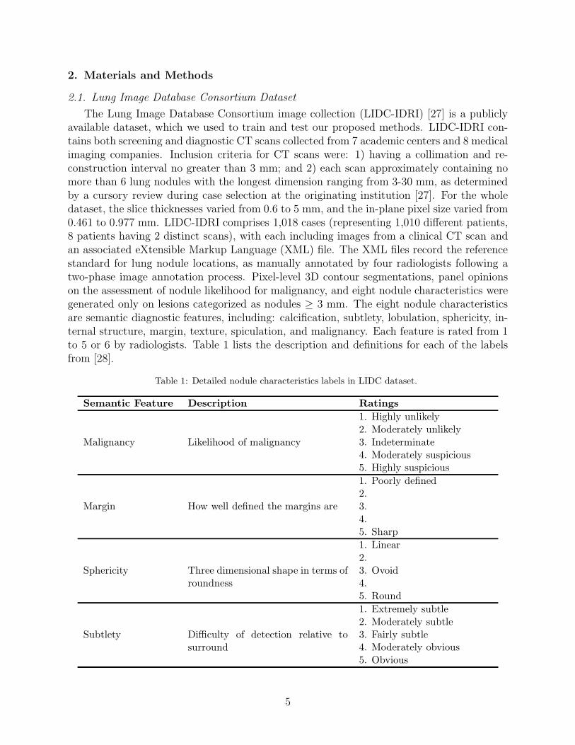
The Lung Image Database Consortium image collection (LIDC-IDRI) [27] is a publiclyavailable dataset, which we used to train and test our proposed methods. LIDC-IDRI con-tains both screening and diagnostic CT scans collected from 7 academic centers and 8 medicalimaging companies. Inclusion criteria for CT scans were: 1) having a collimation and re-construction interval no greater than 3 mm; and 2) each scan approximately containing nomore than 6 lung nodules with the longest dimension ranging from 3-30 mm, as determinedby a cursory review during case selection at the originating institution [27]. For the wholedataset, the slice thicknesses varied from 0.6 to 5 mm, and the in-plane pixel size varied from0.461 to 0.977 mm. LIDC-IDRI comprises 1,018 cases (representing 1,010 different patients,8 patients having 2 distinct scans), with each including images from a clinical CT scan andan associated eXtensible Markup Language (XML) file. The XML files record the referencestandard for lung nodule locations, as manually annotated by four radiologists following atwo-phase image annotation process. Pixel-level 3D contour segmentations, panel opinionson the assessment of nodule likelihood for malignancy, and eight nodule characteristics weregenerated only on lesions categorized as nodules ≥ 3 mm. The eight nodule characteristicsare semantic diagnostic features, including: calcification, subtlety, lobulation, sphericity, in-ternal structure, margin, texture, spiculation, and malignancy. Each feature is rated from 1to 5 or 6 by radiologists. Table 1 lists the description and definitions for each of the labelsfrom [28].

Table 1: Detailed nodule characteristics labels in LIDC dataset.

Semantic Feature Description Ratings

Malignancy Likelihood of malignancy

1. Highly unlikely2. Moderately unlikely3. Indeterminate4. Moderately suspicious5. Highly suspicious

Margin How well defined the margins are

1. Poorly defined2.3.4.5. Sharp

Sphericity Three dimensional shape in terms ofroundness

1. Linear2.3. Ovoid4.5. Round

Subtlety Difficulty of detection relative tosurround

1. Extremely subtle2. Moderately subtle3. Fairly subtle4. Moderately obvious5. Obvious

5

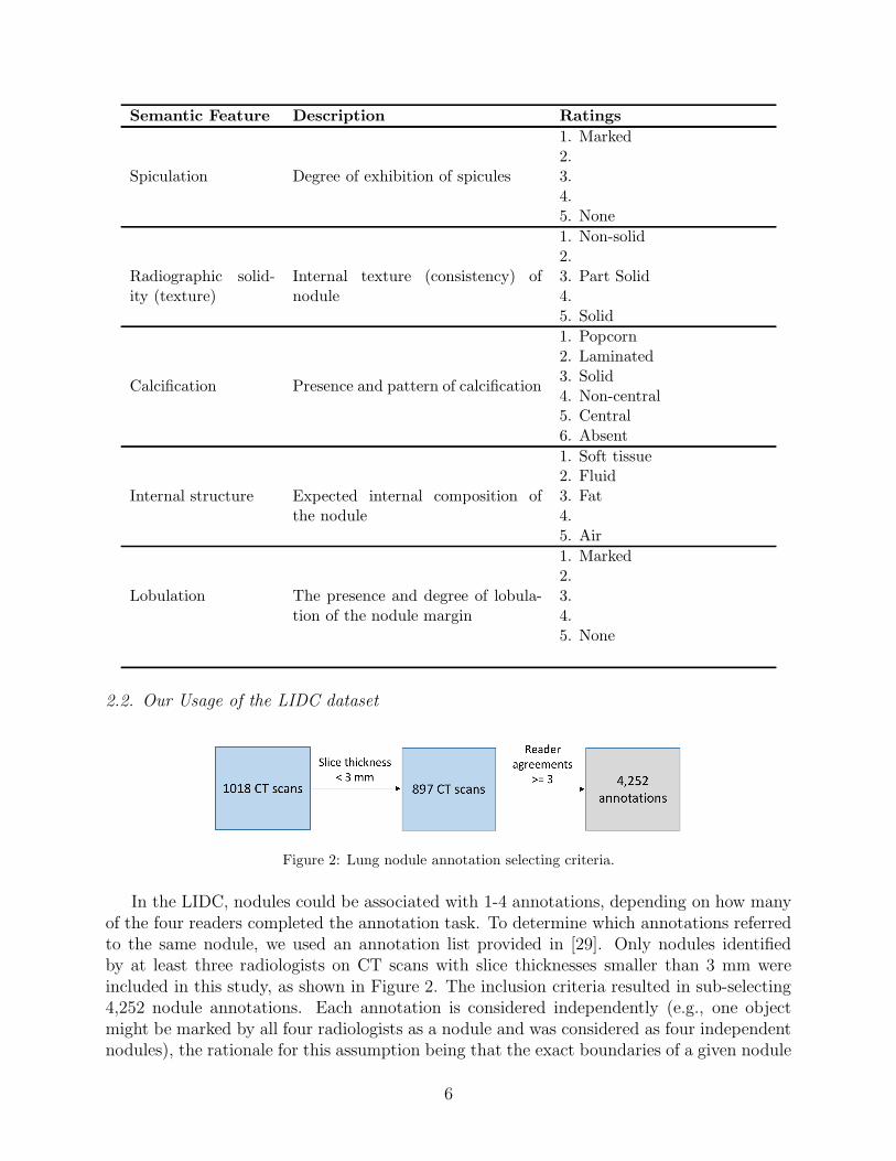
Semantic Feature Description Ratings

Spiculation Degree of exhibition of spicules

1. Marked2.3.4.5. None

Radiographic solid-ity (texture)

Internal texture (consistency) ofnodule

1. Non-solid2.3. Part Solid4.5. Solid

Calcification Presence and pattern of calcification

1. Popcorn2. Laminated3. Solid4. Non-central5. Central6. Absent

Internal structure Expected internal composition ofthe nodule

1. Soft tissue2. Fluid3. Fat4.5. Air

Lobulation The presence and degree of lobula-tion of the nodule margin

1. Marked2.3.4.5. None

2.2. Our Usage of the LIDC dataset

Figure 2: Lung nodule annotation selecting criteria.

In the LIDC, nodules could be associated with 1-4 annotations, depending on how manyof the four readers completed the annotation task. To determine which annotations referredto the same nodule, we used an annotation list provided in [29]. Only nodules identifiedby at least three radiologists on CT scans with slice thicknesses smaller than 3 mm wereincluded in this study, as shown in Figure 2. The inclusion criteria resulted in sub-selecting4,252 nodule annotations. Each annotation is considered independently (e.g., one objectmight be marked by all four radiologists as a nodule and was considered as four independentnodules), the rationale for this assumption being that the exact boundaries of a given nodule

6

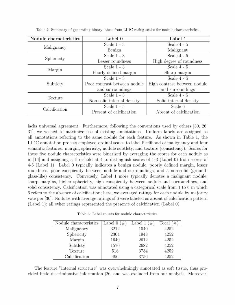
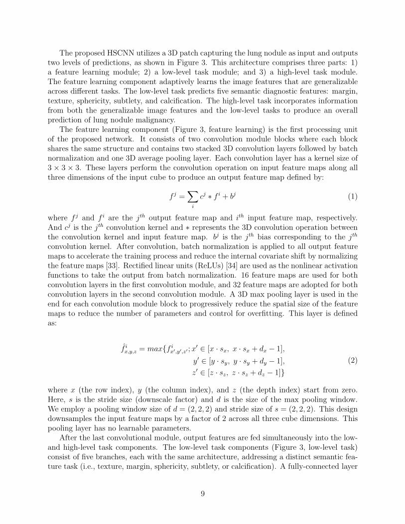
Table 2: Summary of generating binary labels from LIDC rating scales for nodule characteristics.

Nodule characteristics Label 0 Label 1

MalignancyScale 1 - 3Benign

Scale 4 - 5Malignant

SphericityScale 1 - 3

Lesser roundnessScale 4 - 5

High degree of roundness

MarginScale 1 - 3

Poorly defined marginScale 4 - 5

Sharp margin

SubtletyScale 1 - 3

Poor contrast between noduleand surroundings

Scale 4 - 5High contrast between nodule

and surroundings

TextureScale 1 - 3

Non-solid internal densityScale 4 - 5

Solid internal density

CalcificationScale 1 - 5

Present of calcificationScale 6

Absent of calcification

lacks universal agreement. Furthermore, following the conventions used by others [30, 26,31], we wished to maximize use of existing annotations. Uniform labels are assigned toall annotations referring to the same nodule for each feature. As shown in Table 1, theLIDC annotation process employed ordinal scales to label likelihood of malignancy and foursemantic features: margin, sphericity, nodule subtlety, and texture (consistency). Scores forthese five nodule characteristics were binarized by averaging the scores for each nodule asin [14] and assigning a threshold at 4 to distinguish scores of 1-3 (Label 0) from scores of4-5 (Label 1). Label 0 typically indicates a benign nodule, poorly defined margin, lesserroundness, poor conspicuity between nodule and surroundings, and a non-solid (ground-glass-like) consistency. Conversely, Label 1 more typically denotes a malignant nodule,sharp margins, higher sphericity, high conspicuity between nodule and surroundings, andsolid consistency. Calcification was annotated using a categorical scale from 1 to 6 in which6 refers to the absence of calcification; here, we averaged ratings for each nodule by majorityvote per [30]. Nodules with average ratings of 6 were labeled as absent of calcification pattern(Label 1); all other ratings represented the presence of calcification (Label 0).

Table 3: Label counts for nodule characteristics.

Nodule characteristics Label 0 (#) Label 1 (#) Total (#)Malignancy 3212 1040 4252Sphericity 2304 1948 4252Margin 1640 2612 4252Subtlety 1570 2682 4252Texture 518 3734 4252

Calcification 496 3756 4252

The feature ”internal structure” was overwhelmingly annotated as soft tissue, thus pro-vided little discriminative information [26] and was excluded from our analysis. Moreover,

7

the Cancer Imaging Archive (TCIA) reported that an indeterminate subset of cases in thedataset were inconsistently annotated with respect to spiculation and lobulation [32]. Assuch, we did not consider these two features in our model. Finally, it should be noted thatthe actual diagnosis of the nodules is not known in the LIDC dataset. For the purposes ofthis work, the likelihood of malignancy served as the proxy for truth. Table 2 summarizesthe generation of the binary labels from LIDC rating scales as described above. Table 3 liststhe data counts for each label of the nodule characteristics.

2.3. Data Preprocessing

The LIDC dataset contains a heterogeneous set of scans obtained using various acqui-sition and reconstruction parameters. To normalize pixel values, all CT scans were firsttransformed to Hounsfield (HU) scales using the information in the DICOM (Digital Imag-ing and Communication in Medicine) series header and converted to a range of (0, 1) from(-1000, 500 HU). A 3D cube of 40 × 40 × 40 mm were extracted for each candidate. Eachcube was centered around the candidate. 40 mm was chosen so that all candidates wouldbe fully contained in this cube as the largest nodules in our subset were maximally 30 mm.We then rescaled each cube to a fixed size of pixels in all three dimensions, resulting inisotropic cubes for all cases. This preprocessing method retained the original relative nodulesize information, which is considered useful domain knowledge for the the following tasks.

2.4. Hierarchical Semantic Convolutional Neural Network

Figure 3: Model architecture of the hierarchical semantic convolutional neural network.

8

The proposed HSCNN utilizes a 3D patch capturing the lung nodule as input and outputstwo levels of predictions, as shown in Figure 3. This architecture comprises three parts: 1)a feature learning module; 2) a low-level task module; and 3) a high-level task module.The feature learning component adaptively learns the image features that are generalizableacross different tasks. The low-level task predicts five semantic diagnostic features: margin,texture, sphericity, subtlety, and calcification. The high-level task incorporates informationfrom both the generalizable image features and the low-level tasks to produce an overallprediction of lung nodule malignancy.

The feature learning component (Figure 3, feature learning) is the first processing unitof the proposed network. It consists of two convolution module blocks where each blockshares the same structure and contains two stacked 3D convolution layers followed by batchnormalization and one 3D average pooling layer. Each convolution layer has a kernel size of3 × 3 × 3. These layers perform the convolution operation on input feature maps along allthree dimensions of the input cube to produce an output feature map defined by:

f j =∑

i

cj ∗ f i + bj (1)

where f j and f i are the jth output feature map and ith input feature map, respectively.And cj is the jth convolution kernel and ∗ represents the 3D convolution operation betweenthe convolution kernel and input feature map. bj is the jth bias corresponding to the jth

convolution kernel. After convolution, batch normalization is applied to all output featuremaps to accelerate the training process and reduce the internal covariate shift by normalizingthe feature maps [33]. Rectified linear units (ReLUs) [34] are used as the nonlinear activationfunctions to take the output from batch normalization. 16 feature maps are used for bothconvolution layers in the first convolution module, and 32 feature maps are adopted for bothconvolution layers in the second convolution module. A 3D max pooling layer is used in theend for each convolution module block to progressively reduce the spatial size of the featuremaps to reduce the number of parameters and control for overfitting. This layer is definedas:

f ix,y,z = max{f i

x′,y′,z′; x′ ∈ [x · sx, x · sx + dx − 1],

y′ ∈ [y · sy, y · sy + dy − 1],

z′ ∈ [z · sz, z · sz + dz − 1]}

(2)

where x (the row index), y (the column index), and z (the depth index) start from zero.Here, s is the stride size (downscale factor) and d is the size of the max pooling window.We employ a pooling window size of d = (2, 2, 2) and stride size of s = (2, 2, 2). This designdownsamples the input feature maps by a factor of 2 across all three cube dimensions. Thispooling layer has no learnable parameters.

After the last convolutional module, output features are fed simultaneously into the low-and high-level task components. The low-level task components (Figure 3, low-level task)consist of five branches, each with the same architecture, addressing a distinct semantic fea-ture task (i.e., texture, margin, sphericity, subtlety, or calcification). A fully-connected layer

9

(densely-connected) is the major basic building block for each of these branches. One fully-connected layer connects each input unit to each output unit, designed to capture correlationsfrom all input feature units to the output. Batch normalization and dropout techniques areboth used to control model overfitting. The dropout method randomly removes connectionsbetween input and output units during network training to prevent units from co-adaptingtoo much [35]. Two fully-connected layers are employed before the final binary predictionwith 256 neurons and 64 neurons for the first and second layer, respectively.

The high-level task component (Figure 3, high-level task) predicts the lung nodule ma-lignancy as the final task. This module concatenates as input the output features from thefeature learning component and each of the low-level task branches. As shown in Figure 3,the output feature maps from the last convolution module of the feature learning componentare used, along with the output from the last second fully-connected layer of each subtaskbranch. This design makes the final prediction utilize the basic features learned from theshared convolution modules, and forces the convolution blocks to extract representationsthat are generalizable across tasks. It also makes use of the information learned from eachrelated explainable subtask to ultimately infer nodule malignancy. The last fully-connectedlayer in each subtask branch is trained to extract representations more specific to the corre-sponding subtask compared to the second to last fully-connected layer. Thus, the second tolast layer of the subtask branch is chosen to provide less specific but salient information forthe final malignancy prediction task. The concatenated features are inputted into a fully-connected layer with 256 neurons, followed by a batch normalization operation before thefinal malignancy prediction.

To jointly optimize the the HSCNN during the network training, a global loss functionis proposed to maximize the probability of predicting the correct label for each task by:

Lglobal =1

N

N∑

i=1

(

5∑

j=1

λj · Lj,i + LM,i) (3)

where N is the total number of training samples and i indicates the ith training sample. j isthe jth subtask and j ∈ [1, 5]. λj is the weighting hyperparameter for the jth subtask. Lj,i

represents the loss for sample i and task j. LM,i is the loss for the malignancy predictiontask for the ith sample. Each loss component is defined as weighted cross entropy loss by:

Lj,i = − log (efyi,j/∑

n

efyn,j ) · ωyi,j (4)

where yi is true label for the ith sample (xi, yi). Here, yi equals 0 or 1. fyi,j is the prediction

score of the true class yi for task j and fyn,j represents a prediction score for class yn. We useωyi,j to represent the weight of class yi for task j. The use of ωyi,j is important because the la-bels are imbalanced in all the tasks and ωyi,j is helpful in reducing the training bias introducedby such data imbalance. Specifically, ωyi,j weights each class loss proportional to the recipro-cal of the class counts in the training data. For instance, ωyi=0,j = Nyi=1,j/(Nyi=0,j +Nyi=1,j)and ωyi=1,j = Nyi=0,j/(Nyi=0,j + Nyi=1,j). Nyi=1,j represents the total count of samples inthe training data for task j, where the true class label equals 1. The global loss function isminimized during the training process by iteratively computing the gradient of Lglobal overthe learnable parameters of HSCNN and updates the parameters through back-propagation.

10

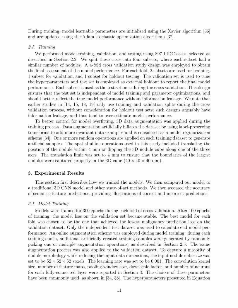
During training, model learnable parameters are initialized using the Xavier algorithm [36]and are updated using the Adam stochastic optimization algorithom [37].

2.5. Training

We performed model training, validation, and testing using 897 LIDC cases, selected asdescribed in Section 2.2. We split these cases into four subsets, where each subset had asimilar number of nodules. A 4-fold cross validation study design was employed to obtainthe final assessment of the model performance. For each fold, 2 subsets are used for training,1 subset for validation, and 1 subset for holdout testing. The validation set is used to tunethe hyperparameters and test set is employed as external holdout to report the final modelperformance. Each subset is used as the test set once during the cross validation. This designensures that the test set is independent of model training and parameter optimizations, andshould better reflect the true model performance without information leakage. We note thatearlier studies in [14, 15, 18, 19] only use training and validation splits during the crossvalidation process, without consideration for holdout test sets; such designs arguably haveinformation leakage, and thus tend to over-estimate model performance.

To better control for model overfitting, 3D data augmentation was applied during thetraining process. Data augmentation artificially inflates the dataset by using label-preservingtransforms to add more invariant data examples and is considered as a model regularizationscheme [34]. One or more random operations are applied on each training dataset to generateartificial samples. The spatial affine operations used in this study included translating theposition of the nodule within 4 mm or flipping the 3D nodule cube along one of the threeaxes. The translation limit was set to 4 mm to ensure that the boundaries of the largestnodules were captured properly in the 3D cube (40× 40× 40 mm).

3. Experimental Results

This section first describes how we trained the models. We then compared our model toa traditional 3D CNN model and other state-of-art methods. We then assessed the accuracyof semantic feature predictions, providing illustrations of correct and incorrect predictions.

3.1. Model Training

Models were trained for 300 epochs during each fold of cross-validation. After 100 epochsof training, the model loss on the validation set became stable. The best model for eachfold was chosen to be the one that achieved the lowest malignancy prediction loss on thevalidation dataset. Only the independent test dataset was used to calculate end model per-formance. An online augmentation scheme was employed during model training: during eachtraining epoch, additional artificially created training samples were generated by randomlypicking one or multiple augmentation operations, as described in Section 2.5. The sameaugmentation process was also applied to the validation dataset. To capture a majority ofnodule morphology while reducing the input data dimensions, the input nodule cube size wasset to be 52× 52× 52 voxels. The learning rate was set to be 0.001. The convolution kernelsize, number of feature maps, pooling window size, downscale factor, and number of neuronsfor each fully-connected layer were reported in Section 3. The choices of these parametershave been commonly used, as shown in [34, 38]. The hyperparameters presented in Equation

11

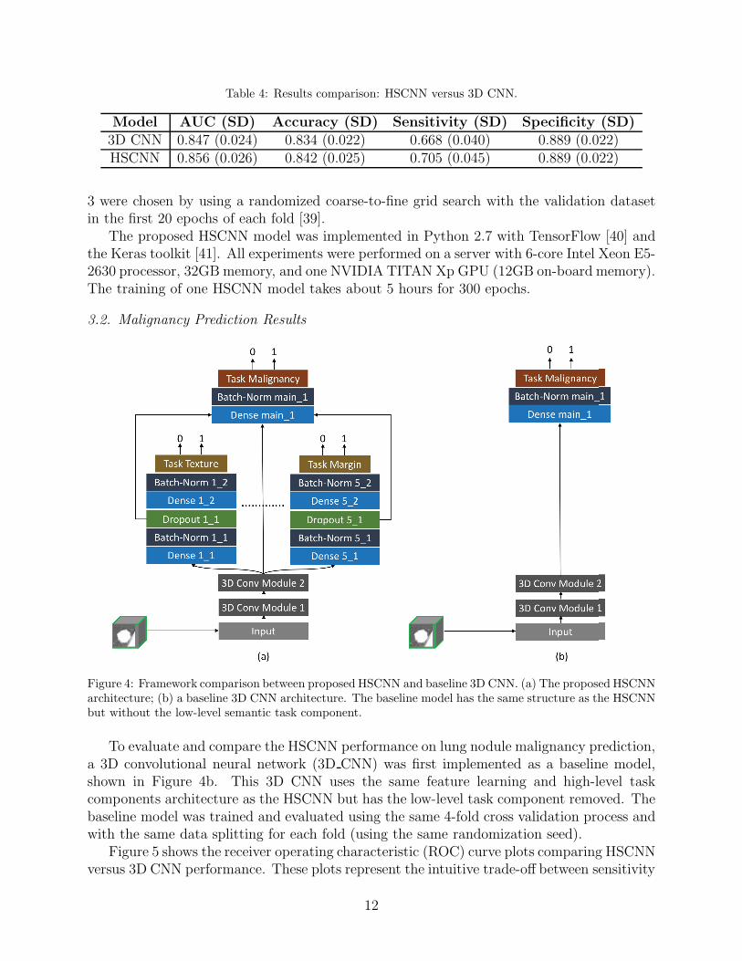
Table 4: Results comparison: HSCNN versus 3D CNN.

Model AUC (SD) Accuracy (SD) Sensitivity (SD) Specificity (SD)3D CNN 0.847 (0.024) 0.834 (0.022) 0.668 (0.040) 0.889 (0.022)HSCNN 0.856 (0.026) 0.842 (0.025) 0.705 (0.045) 0.889 (0.022)

3 were chosen by using a randomized coarse-to-fine grid search with the validation datasetin the first 20 epochs of each fold [39].

The proposed HSCNN model was implemented in Python 2.7 with TensorFlow [40] andthe Keras toolkit [41]. All experiments were performed on a server with 6-core Intel Xeon E5-2630 processor, 32GB memory, and one NVIDIA TITAN Xp GPU (12GB on-board memory).The training of one HSCNN model takes about 5 hours for 300 epochs.

3.2. Malignancy Prediction Results

Figure 4: Framework comparison between proposed HSCNN and baseline 3D CNN. (a) The proposed HSCNNarchitecture; (b) a baseline 3D CNN architecture. The baseline model has the same structure as the HSCNNbut without the low-level semantic task component.

To evaluate and compare the HSCNN performance on lung nodule malignancy prediction,a 3D convolutional neural network (3D CNN) was first implemented as a baseline model,shown in Figure 4b. This 3D CNN uses the same feature learning and high-level taskcomponents architecture as the HSCNN but has the low-level task component removed. Thebaseline model was trained and evaluated using the same 4-fold cross validation process andwith the same data splitting for each fold (using the same randomization seed).

Figure 5 shows the receiver operating characteristic (ROC) curve plots comparing HSCNNversus 3D CNN performance. These plots represent the intuitive trade-off between sensitivity

12

Figure 5: Receiver operating characteristic curve comparison: HSCNN versus 3D CNN. The AUC of 3DHSCNN is significantly higher than 3D CNN according to a paired T-test as shown in Table 5.

and specificity. By visual inspection of the ROC curves, HSCNN performs better than thetraditional 3D CNN model. The area under the ROC curve (AUC) quantitatively comparesthe overall performance of a classification model and is frequently used as a metric to accessperformance in nodule classification [15, 17, 26, 30, 31]. Table 5 summarizes the mean AUCscore, accuracy, sensitivity, and specificity for both models. The HSCNN model achieved amean AUC 0.856, mean accuracy 0.842, mean sensitivity 0.705 and mean specificity 0.889;while the 3D CNN model achieved a mean AUC 0.847, mean accuracy 0.834, mean sensitiv-ity 0.668 and mean specificity 0.889. Both ROC plots and metric assessments show that theproposed HSCNN achieved better performance for malignancy prediction compared with theconventional 3D CNN approach.

To assess the statistical significance of model performance improvements, we conducteda paired sample t-test to evaluate the mean differences in AUC scores between the HSCNNand 3D CNN model. Group 1 consists of the AUC score of the HSCNN model for eachholdout test fold during the cross validation. Group 2 consists of the corresponding AUCscore for the 3D CNN for the same fold. The null hypothesis is that the mean difference ofAUC score between these two models equals 0. Table 5 summarizes the AUC scores for thesegroups and results of a paired t-test. The test obtained a p-value of 0.005 and confidenceinterval of [0.0051, 0.0129], thus rejecting the null hypothesis and indicating that the HSCNNmodel achieved a statistically significantly better AUC relative to the 3D CNN. The meanimprovement of the AUC score was 0.009. This finding demonstrates that adding a low-leveltask component on an existing CNN structure may improve the prediction of malignancy ina lung nodule.

We also compared our results with current deep learning models for lung nodule malig-

13

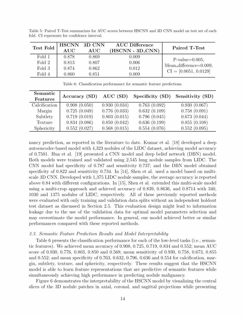
Table 5: Paired T-Test summarizes for AUC scores between HSCNN and 3D CNN model on test set of eachfold. CI represents for confidence interval.

Test FoldHSCNNAUC

3D CNNAUC

AUC Difference(HSCNN - 3D CNN)

Paired T-Test

Fold 1 0.878 0.869 0.009P-value=0.005,

Mean difference=0.009,CI = [0.0051, 0.0129]

Fold 2 0.813 0.807 0.006Fold 3 0.874 0.862 0.012Fold 4 0.860 0.851 0.009

Table 6: Classification performance for semantic feature predictions.

SemanticFeatures

Accuracy (SD) AUC (SD) Specificity (SD) Sensitivity (SD)

Calcification 0.908 (0.050) 0.930 (0.034) 0.763 (0.092) 0.930 (0.067)Margin 0.725 (0.049) 0.776 (0.033) 0.632 (0.109) 0.758 (0.091)Subtlety 0.719 (0.019) 0.803 (0.015) 0.796 (0.045) 0.673 (0.044)Texture 0.834 (0.086) 0.850 (0.042) 0.636 (0.199) 0.855 (0.108)Sphericity 0.552 (0.027) 0.568 (0.015) 0.554 (0.076) 0.552 (0.095)

nancy prediction, as reported in the literature to date. Kumar et al. [18] developed a deepautoencoder-based model with 4,323 nodules of the LIDC dataset, achieving model accuracyof 0.7501. Hua et al. [19] presented a CNN model and deep belief network (DBN) model.Both models were trained and validated using 2,545 lung nodule samples from LIDC. TheCNN model had specificity of 0.787 and sensitivity 0.737; and the DBN model obtainedspecificity of 0.822 and sensitivity 0.734. In [14], Shen et al. used a model based on multi-scale 3D CNN. Developed with 1,375 LIDC nodule samples, the average accuracy is reportedabove 0.84 with different configurations. In [15], Shen et al. extended this multi-scale modelusing a multi-crop approach and achieved accuracy of 0.839, 0.8636, and 0.8714 with 340,1030 and 1375 nodules of LIDC, respectively. All of these previously reported methodswere evaluated with only training and validation data splits without an independent holdouttest dataset as discussed in Section 2.5. This evaluation design might lead to informationleakage due to the use of the validation data for optimal model parameters selection andmay overestimate the model performance. In general, our model achieved better or similarperformances compared with these reported methods.

3.3. Semantic Feature Prediction Results and Model Interpretability

Table 6 presents the classification performance for each of the low-level tasks (i.e., seman-tic features). We achieved mean accuracy of 0.908, 0.725, 0.719, 0.834 and 0.552; mean AUCscore of 0.930, 0.776, 0.803, 0.850 and 0.568; mean sensitivity of 0.930, 0.758, 0.673, 0.855and 0.552; and mean specificity of 0.763, 0.632, 0.796, 0.636 and 0.554 for calcification, mar-gin, subtlety, texture, and sphericity, respectively. These results suggest that the HSCNNmodel is able to learn feature representations that are predictive of semantic features whilesimultaneously achieving high performance in predicting nodule malignancy.

Figure 6 demonstrates the interpretability of the HSCNN model by visualizing the centralslices of the 3D nodule patches in axial, coronal, and sagittal projections while presenting

14

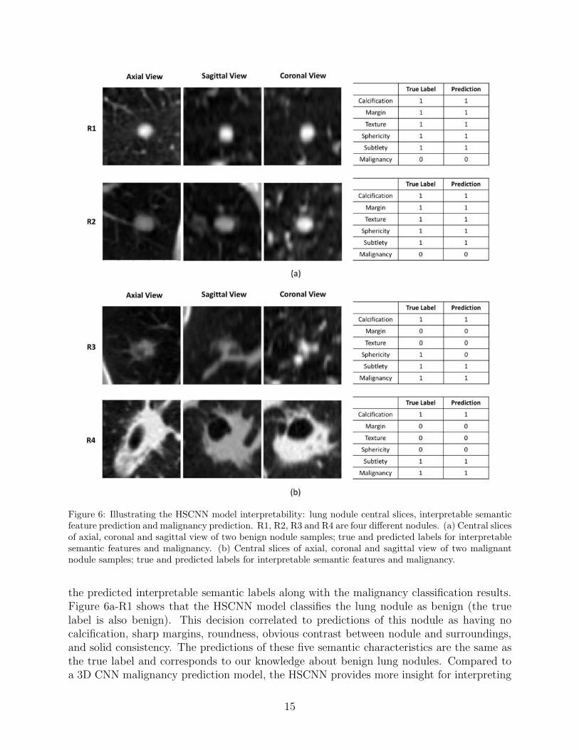
Figure 6: Illustrating the HSCNN model interpretability: lung nodule central slices, interpretable semanticfeature prediction and malignancy prediction. R1, R2, R3 and R4 are four different nodules. (a) Central slicesof axial, coronal and sagittal view of two benign nodule samples; true and predicted labels for interpretablesemantic features and malignancy. (b) Central slices of axial, coronal and sagittal view of two malignantnodule samples; true and predicted labels for interpretable semantic features and malignancy.

the predicted interpretable semantic labels along with the malignancy classification results.Figure 6a-R1 shows that the HSCNN model classifies the lung nodule as benign (the truelabel is also benign). This decision correlated to predictions of this nodule as having nocalcification, sharp margins, roundness, obvious contrast between nodule and surroundings,and solid consistency. The predictions of these five semantic characteristics are the same asthe true label and corresponds to our knowledge about benign lung nodules. Compared toa 3D CNN malignancy prediction model, the HSCNN provides more insight for interpreting

15

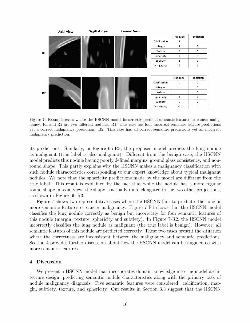
Figure 7: Example cases where the HSCNN model incorrectly predicts semantic features or cancer malig-nancy. R1 and R2 are two different nodules. R1: This case has four incorrect semantic feature predictionsyet a correct malignancy prediction. R2: This case has all correct semantic predictions yet an incorrectmalignancy prediction.

its predictions. Similarly, in Figure 6b-R3, the proposed model predicts the lung noduleas malignant (true label is also malignant). Different from the benign case, the HSCNNmodel predicts this nodule having poorly defined margins, ground glass consistency, and non-round shape. This partly explains why the HSCNN makes a malignancy classification withsuch nodule characteristics corresponding to our expert knowledge about typical malignantnodules. We note that the sphericity predictions made by the model are different from thetrue label. This result is explained by the fact that while the nodule has a more regularround shape in axial view, the shape is actually more elongated in the two other projections,as shown in Figure 6b-R3.

Figure 7 shows two representative cases where the HSCNN fails to predict either one ormore semantic features or cancer malignancy. Figure 7-R1 shows that the HSCNN modelclassifies the lung nodule correctly as benign but incorrectly for four semantic features ofthis nodule (margin, texture, sphericity and subtlety). In Figure 7-R2, the HSCNN modelincorrectly classifies the lung nodule as malignant (the true label is benign). However, allsemantic features of this nodule are predicted correctly. These two cases present the situationwhere the correctness are inconsistent between the malignancy and semantic predictions.Section 4 provides further discussion about how the HSCNN model can be augmented withmore semantic features.

4. Discussion

We present a HSCNN model that incorporates domain knowledge into the model archi-tecture design, predicting semantic nodule characteristics along with the primary task ofnodule malignancy diagnosis. Five semantic features were considered: calcification, mar-gin, subtlety, texture, and sphericity. Our results in Section 3.3 suggest that the HSCNN

16

model quantifies these nodule characteristics in a fully data-driven way yet in one integratedmodel that predicts nodule malignancy. The semantic labels are useful in interpreting themodel’s predictions for malignancy, mapping the features used by the network to predict thehigh-level task with established domain knowledge about pulmonary nodules. Section 3.2shows that this design of the HSCNN also improves the model performance for lung cancermalignancy classification. This study focuses mainly on exploring the values that are addedby incorporating the low-level semantic task component design into the CNN architecture.Further optimization of the network architecture to achieve higher prediction performancecan be performed. For instance, densely connected designs [42] and residual designs [43]could be used to potentially improve model performance. But due to limitations of com-putation power, not all designs are optimally searched; we will investigate these as part offuture work.

There are some limitations to this study. Our semantic labels did not include those ofknown higher association with malignancy, such as nodule size, margin spiculation, lobula-tion, and anatomic location, which have previously been reported as informative [44, 45].In the case of lobulation and spiculation, known labeling errors in the LIDC dataset madethem unsuitable for our use. Additionally, semantic labels are subject to moderate inter-reader variability; performance might be enhanced by limiting semantic labels to those onwhich there is high reader agreement. Third, the malignancy labels provided in the LIDCdataset do not reflect pathological diagnosis but rather, suspicion levels of the interpretingradiologists. Finally, the original semantic features have scales of 5 or 6; binarizing the labelsmay lose some of the semantic information. Changing the threshold for binary classificationwould also affect results. Our rationale for binary labels in this case was to overcome datasparsity, where the number of cases labeled for certain scales might be very small comparedwith the other scales (e.g., only 11 cases are labeled as linear for sphericity out of total4252 cases). Moreover, analysis shows that inter-reader agreement is much lower for 5 or6 scales compared with the proposed binary labels. Thus, binary labeling helps to reducelabeling noise caused by inter-reader variability. These limitations may be circumvented bytraining on large datasets that have been systematically annotated using a shared lexiconthat includes discriminating features. In future work we will explore model improvementby including discriminating semantic features, and investigate model variability using dif-ferent semantic labeling schemes. Although only five subtask modules are presented for theHSCNN architecture in this paper, the HSCNN framework and global loss function couldbe easily extended to increase or decrease the number of low-level semantic features. Thisstudy also paves the way to apply this idea in other disease domain to build interpretablemodels.

5. Conclusion

In this paper, we have developed a novel radiologist-interpretable HSCNN model forpredicting lung cancer in CT-detected indeterminate nodules. This model is able to simul-taneously predict nodule malignancy while classifying five nodule semantic characteristics,including calcification, margin, subtlety, texture, and sphericity of nodules. These diagnosticsemantic features predictions are intermediate outputs associated with the final malignancyprediction, and are useful to explain the diagnosis prediction. Information from each low-

17

level semantic feature prediction is incorporated into the malignancy prediction task byemploying jump connections. This framework is able to enforce the shared basic convolutionmodules in the HSCNN to learn features that are generalizable across tasks. This unifiedmodel is trained by minimizing a joint global loss function, where the losses of both malig-nancy and semantic feature prediction tasks are incorporated. Extensive experiments andstatistical tests show that the proposed HSCNN model is able to significantly improve theclassification performance for nodule malignancy prediction and the semantic characteristicspredictions have improved the model interpretability. This trained model could also serveas a lung nodule semantic feature generator.

Author Contributions

All authors contributed to the development of the project. SS developed the methodology,conducted the experiments and wrote the manuscript. SXH contributed to the experiments.AATB and DRA provided valuable advice and domain input. WH provided oversight overthe project and contributed to its design. All authors reviewed the manuscript.

Acknowledgement

The authors acknowledge the National Cancer Institute and the Foundation for the Na-tional Institutes of Health, and their critical role in the creation of the free publicly availableLIDC/IDRI Database used in this study. Research reported in this publication was partlysupported by the National Cancer Institute of the National Institutes of Health under awardnumber R01 CA210360, the Center for Domain-Specific Computing (CDSC) funded by theNSF Expedition in Computing Award CCF-0926127, and the National Science Foundationunder Grant No. 1722516. Computing resources were provided by the NIH Data CommonsPilot and a donation of a TITAN Xp graphics card by the NVIDIA Corporation. The con-tent is solely the responsibility of the authors and does not necessarily represent the officialviews of sponsor agencies.

18

References

References

[1] L. A. Torre, R. L. Siegel, A. Jemal, Lung cancer statistics, in: Lung Cancer andPersonalized Medicine, Springer, 2016, pp. 1–19.

[2] S. Shen, S. X. Han, P. Petousis, R. E. Weiss, F. Meng, A. A. Bui, W. Hsu, A bayesianmodel for estimating multi-state disease progression, Computers in biology and medicine81 (2017) 111–120.

[3] N. L. S. T. R. Team, et al., Reduced lung-cancer mortality with low-dose computedtomographic screening, N Engl J Med 2011 (2011) 395–409.

[4] K. ten Haaf, J. Jeon, M. C. Tammemagi, S. S. Han, C. Y. Kong, S. K. Plevritis, E. J.Feuer, H. J. de Koning, E. W. Steyerberg, R. Meza, Risk prediction models for selectionof lung cancer screening candidates: A retrospective validation study, PLoS medicine14 (2017) e1002277.

[5] B. Zhao, Y. Tan, D. J. Bell, S. E. Marley, P. Guo, H. Mann, M. L. Scott, L. H. Schwartz,D. C. Ghiorghiu, Exploring intra-and inter-reader variability in uni-dimensional, bi-dimensional, and volumetric measurements of solid tumors on ct scans reconstructed atdifferent slice intervals, European journal of radiology 82 (2013) 959–968.

[6] S. G. Armato, M. B. Altman, J. Wilkie, S. Sone, F. Li, A. S. Roy, et al., Automatedlung nodule classification following automated nodule detection on ct: A serial approach,Medical Physics 30 (2003) 1188–1197.

[7] S. Shen, A. A. Bui, J. Cong, W. Hsu, An automated lung segmentation approach usingbidirectional chain codes to improve nodule detection accuracy, Computers in biologyand medicine 57 (2015) 139–149.

[8] N. Duggan, E. Bae, S. Shen, W. Hsu, A. Bui, E. Jones, M. Glavin, L. Vese, A techniquefor lung nodule candidate detection in ct using global minimization methods, in: Inter-national Workshop on Energy Minimization Methods in Computer Vision and PatternRecognition, Springer, pp. 478–491.

[9] M. Firmino, G. Angelo, H. Morais, M. R. Dantas, R. Valentim, Computer-aided detec-tion (cade) and diagnosis (cadx) system for lung cancer with likelihood of malignancy,Biomedical engineering online 15 (2016) 2.

[10] G. J. Amir, H. P. Lehmann, After detection:: The improved accuracy of lung cancerassessment using radiologic computer-aided diagnosis, Academic radiology 23 (2016)186–191.

[11] P. Huang, S. Park, R. Yan, J. Lee, L. C. Chu, C. T. Lin, A. Hussien, J. Rathmell,B. Thomas, C. Chen, et al., Added value of computer-aided ct image features for earlylung cancer diagnosis with small pulmonary nodules: A matched case-control study,Radiology 286 (2017) 286–295.

19

[12] D. Zinovev, J. Feigenbaum, J. Furst, D. Raicu, Probabilistic lung nodule classificationwith belief decision trees, in: Engineering in medicine and biology society, EMBC, 2011annual international conference of the IEEE, IEEE, pp. 4493–4498.

[13] T. W. Way, B. Sahiner, H.-P. Chan, L. Hadjiiski, P. N. Cascade, A. Chughtai, N. Bogot,E. Kazerooni, Computer-aided diagnosis of pulmonary nodules on ct scans: Improve-ment of classification performance with nodule surface features, Medical physics 36(2009) 3086–3098.

[14] W. Shen, M. Zhou, F. Yang, C. Yang, J. Tian, Multi-scale convolutional neural networksfor lung nodule classification, in: International Conference on Information Processingin Medical Imaging, Springer, pp. 588–599.

[15] W. Shen, M. Zhou, F. Yang, D. Yu, D. Dong, C. Yang, Y. Zang, J. Tian, Multi-cropconvolutional neural networks for lung nodule malignancy suspiciousness classification,Pattern Recognition 61 (2017) 663–673.

[16] E. A. R. Piedra, R. K. Taira, S. El-Saden, B. M. Ellingson, A. A. Bui, W. Hsu, Assessingvariability in brain tumor segmentation to improve volumetric accuracy and character-ization of change, in: Biomedical and Health Informatics (BHI), 2016 IEEE-EMBSInternational Conference on, IEEE, pp. 380–383.

[17] F. Ciompi, B. de Hoop, S. J. van Riel, K. Chung, E. T. Scholten, M. Oudkerk, P. A.de Jong, M. Prokop, B. van Ginneken, Automatic classification of pulmonary peri-fissural nodules in computed tomography using an ensemble of 2d views and a convolu-tional neural network out-of-the-box, Medical image analysis 26 (2015) 195–202.

[18] D. Kumar, A. Wong, D. A. Clausi, Lung nodule classification using deep features in ctimages, in: Computer and Robot Vision (CRV), 2015 12th Conference on, IEEE, pp.133–138.

[19] K.-L. Hua, C.-H. Hsu, S. C. Hidayati, W.-H. Cheng, Y.-J. Chen, Computer-aided clas-sification of lung nodules on computed tomography images via deep learning technique,OncoTargets and therapy 8 (2015).

[20] A. Farag, A. Ali, J. Graham, A. Farag, S. Elshazly, R. Falk, Evaluation of geometricfeature descriptors for detection and classification of lung nodules in low dose ct scansof the chest, in: Biomedical Imaging: From Nano to Macro, 2011 IEEE InternationalSymposium on, IEEE, pp. 169–172.

[21] P.-L. Lin, P.-W. Huang, C.-H. Lee, M.-T. Wu, Automatic classification for solitarypulmonary nodule in ct image by fractal analysis based on fractional brownian motionmodel, Pattern Recognition 46 (2013) 3279–3287.

[22] W. Jorritsma, F. Cnossen, P. van Ooijen, Improving the radiologist–cad interaction:designing for appropriate trust, Clinical radiology 70 (2015) 115–122.

20

[23] H. Kim, C. M. Park, J. M. Goo, J. E. Wildberger, H.-U. Kauczor, Quantitative com-puted tomography imaging biomarkers in the diagnosis and management of lung cancer,Investigative radiology 50 (2015) 571–583.

[24] J. J. Erasmus, J. E. Connolly, H. P. McAdams, V. L. Roggli, Solitary pulmonarynodules: Part i. morphologic evaluation for differentiation of benign and malignantlesions, Radiographics 20 (2000) 43–58.

[25] A. Kaya, A. B. Can, A weighted rule based method for predicting malignancy ofpulmonary nodules by nodule characteristics, Journal of biomedical informatics 56(2015) 69–79.

[26] M. C. Hancock, J. F. Magnan, Lung nodule malignancy classification using onlyradiologist-quantified image features as inputs to statistical learning algorithms: prob-ing the lung image database consortium dataset with two statistical learning methods,Journal of Medical Imaging 3 (2016) 044504.

[27] S. G. Armato, G. McLennan, L. Bidaut, M. F. McNitt-Gray, C. R. Meyer, A. P. Reeves,B. Zhao, D. R. Aberle, C. I. Henschke, E. A. Hoffmoan, et al., The lung image databaseconsortium (lidc) and image database resource initiative (idri): a completed referencedatabase of lung nodules on ct scans, Medical physics 38 (2011) 915–931.

[28] M. F. McNitt-Gray, S. G. Armato, C. R. Meyer, A. P. Reeves, G. McLennan, R. C.Pais, J. Freymann, M. S. Brown, R. M. Engelmann, P. H. Bland, et al., The lung imagedatabase consortium (lidc) data collection process for nodule detection and annotation,Academic radiology 14 (2007) 1464–1474.

[29] A. P. Reeves, A. M. Biancardi, The lung image database consortium (lidc) nodule sizereport, http://www.via.cornell.edu/lidc/, 2011. Release: 2011-10-27-2.

[30] K. Clark, B. Vendt, K. Smith, J. Freymann, J. Kirby, P. Koppel, S. Moore, S. Phillips,D. Maffitt, M. Pringle, et al., The cancer imaging archive (tcia): maintaining andoperating a public information repository, Journal of digital imaging 26 (2013) 1045–1057.

[31] B. R. Froz, A. O. de Carvalho Filho, A. C. Silva, A. C. de Paiva, R. A. Nunes, M. Gat-tass, Lung nodule classification using artificial crawlers, directional texture and supportvector machine, Expert Systems with Applications 69 (2017) 176–188.

[32] The Cancer Imaging Archive, Lung image database consortium - readerannotation and markup - annotation and markup issues/comments,https://wiki.cancerimagingarchive.net/display/Public/LIDC-IDRI, 2017.

[33] S. Ioffe, C. Szegedy, Batch normalization: Accelerating deep network training by re-ducing internal covariate shift, arXiv preprint arXiv:1502.03167 (2015).

[34] A. Krizhevsky, I. Sutskever, G. E. Hinton, Imagenet classification with deep convo-lutional neural networks, in: Advances in neural information processing systems, pp.1097–1105.

21

[35] N. Srivastava, G. Hinton, A. Krizhevsky, I. Sutskever, R. Salakhutdinov, Dropout:A simple way to prevent neural networks from overfitting, The Journal of MachineLearning Research 15 (2014) 1929–1958.

[36] X. Glorot, Y. Bengio, Understanding the difficulty of training deep feedforward neu-ral networks, in: Proceedings of the thirteenth international conference on artificialintelligence and statistics, pp. 249–256.

[37] D. P. Kingma, J. Ba, Adam: A method for stochastic optimization, arXiv preprintarXiv:1412.6980 (2014).

[38] K. Simonyan, A. Zisserman, Very deep convolutional networks for large-scale imagerecognition, CoRR abs/1409.1556 (2014).

[39] J. Bergstra, Y. Bengio, Random search for hyper-parameter optimization, Journal ofMachine Learning Research 13 (2012) 281–305.

[40] M. Abadi, P. Barham, J. Chen, Z. Chen, A. Davis, J. Dean, M. Devin, S. Ghemawat,G. Irving, M. Isard, et al., Tensorflow: A system for large-scale machine learning., in:OSDI, volume 16, pp. 265–283.

[41] F. Chollet, et al., Keras, 2015.

[42] G. Huang, Z. Liu, K. Q. Weinberger, L. van der Maaten, Densely connected convolu-tional networks, arXiv preprint arXiv:1608.06993 (2016).

[43] K. He, X. Zhang, S. Ren, J. Sun, Deep residual learning for image recognition, in:Proceedings of the IEEE Conference on Computer Vision and Pattern Recognition, pp.770–778.

[44] A. McWilliams, M. C. Tammemagi, J. R. Mayo, H. Roberts, G. Liu, K. Soghrati, K. Ya-sufuku, S. Martel, F. Laberge, M. Gingras, et al., Probability of cancer in pulmonarynodules detected on first screening ct, New England Journal of Medicine 369 (2013)910–919.

[45] S. J. Swensen, M. D. Silverstein, D. M. Ilstrup, C. D. Schleck, E. S. Edell, The proba-bility of malignancy in solitary pulmonary nodules: application to small radiologicallyindeterminate nodules, Archives of internal medicine 157 (1997) 849–855.

22

Conflict of Interest Statement

None Declared.

23