Localization of Humans in Images Using Convolutional ...

Localization of Humans in ImagesUsing Convolutional Networks

by

Jonathan James Richard Tompson

A dissertation submitted in partial fulfillment

of the requirements for the degree of

Doctor of Philosophy

Department of Computer Science

New York University

May 2015

Professor Christoph Bregler

Dedication

To Vanessa, who‘s infinite patience, understanding and love has led me to this point.

ii

Acknowledgements

This work would not have been possible without the guidance and support of many

people, both friends and colleges alike.

Firstly, I would like to thank my family for the many years of love and support;

for being understanding of an overly curious child prone to taking things apart without

putting them back together. In particular I would like to thank my mother and father,

Diane and Phillip, for eventually teaching me how to put it all back together.

I would like to thank Ken Perlin for teaching me the value of truly creative think-

ing and for showing me how a powerful imagination can drive successful research. I

would also like to thank my advisor, Chris Bregler, for many hours spent proof reading

conference submissions at the last minute and for making the whole process a fun and

enjoyable experience. Many thanks to Yann LeCun, who was a constant source of key

insights and invaluable advice, which has help me learn the intuitions that led to much

of the work in this thesis.

Of course there are also many students at NYU who deserve a huge amount of credit

for helping me through my PhD. I would like to thank Murphy Stein for helping me

learn to ask the right questions. I owe a debt of gratitude to Arjun Jain for many, many

hours of insightful discussions, as well as helping me find all those annoying bugs. I

would like to thank Ross Goroshin for teaching me about auto-encoders and all things

“unsupervised” and I would like to thank Kristofer Schlachter for our shared love of

computer graphics.

Lastly, I owe a huge debt of gratitude to Alberto Lerner for teaching me the impor-

tance of detailed-oriented engineering. I am absolutely certain that I would still be a

terrible coder if not for your patients, understanding and “tough love” code reviews.

iii

Abstract

Tracking of humans in images is a long standing problem in computer vision re-

search for which, despite significant research effort, an adequate solution has not yet

emerged. This is largely due to the fact that human body localization is complicated

and difficult; potential solutions must find the location of body joints in images with

invariance to shape, lighting and texture variation and it must do so in the presence of

occlusion and incomplete data. However, despite these significant challenges, this work

will present a framework for human body pose localization that not only offers a signif-

icant improvement over existing traditional architectures, but has sufficient localization

performance and computational efficiency for use in real-world applications.

At its core, this framework makes use of Convolutional Networks to infer the loca-

tion of body joints efficiently and accurately. We describe solutions to two applications

1) hand-tracking from a depth image source and 2) human body-tracking from and RGB

image source. For both these applications we show that Convolutional Networks are able

to significantly out-perform existing state-of-the-art.

We proposes a new hybrid architecture that consists of a deep Convolutional Net-

work and a Probabilistic Graphical Model which can exploit structural domain con-

straints such as geometric relationships between body joint locations to improve track-

ing performance. We then explore the use of both color and motion features to improve

tracking performance. Finally we introduce a novel architecture which includes an ef-

ficient ‘position refinement’ model that is trained to estimate the joint offset location

within a small region of the image. This refinement model allows our network to im-

prove spatial localization accuracy even with large amounts of spatial pooling.

iv

Table of Contents

Dedication . . . . . . . . . . . . . . . . . . . . . . . . . . . . . . . . . . . . ii

Acknowledgements . . . . . . . . . . . . . . . . . . . . . . . . . . . . . . . iii

Abstract . . . . . . . . . . . . . . . . . . . . . . . . . . . . . . . . . . . . . iv

List of Figures . . . . . . . . . . . . . . . . . . . . . . . . . . . . . . . . . . viii

List of Tables . . . . . . . . . . . . . . . . . . . . . . . . . . . . . . . . . . xii

Introduction 1

Related Work 6

I Depth-Based Localization of Human Hands 15

1 Overview 16

2 Hand Tracking Architecture 20

2.1 Binary Classification . . . . . . . . . . . . . . . . . . . . . . . . . . . 20

2.2 Dataset Creation . . . . . . . . . . . . . . . . . . . . . . . . . . . . . . 23

2.3 Feature Detection . . . . . . . . . . . . . . . . . . . . . . . . . . . . . 28

v

2.4 Pose Recovery . . . . . . . . . . . . . . . . . . . . . . . . . . . . . . . 34

3 Experimental Results 37

3.1 Results . . . . . . . . . . . . . . . . . . . . . . . . . . . . . . . . . . . 37

3.2 Future Work . . . . . . . . . . . . . . . . . . . . . . . . . . . . . . . . 44

II RGB-Based Localization of Human Bodies 47

4 Overview 48

4.1 Overview . . . . . . . . . . . . . . . . . . . . . . . . . . . . . . . . . 48

5 Architecture 51

5.1 Model . . . . . . . . . . . . . . . . . . . . . . . . . . . . . . . . . . . 51


6.1 Results . . . . . . . . . . . . . . . . . . . . . . . . . . . . . . . . . . . 65

6.2 Multi-view Motion Capture . . . . . . . . . . . . . . . . . . . . . . . . 68

III Video-based Techniques for Improving Performance 71

7 Overview 72

7.1 Motion Features Overview . . . . . . . . . . . . . . . . . . . . . . . . 72

8 Architecture 74

8.1 Body-Part Detection Model . . . . . . . . . . . . . . . . . . . . . . . . 74


9.1 Results . . . . . . . . . . . . . . . . . . . . . . . . . . . . . . . . . . . 81

vi

IV Efficient Localization in the Presence of Pooling 86

10 Overview 87

10.1 Motivation and Pooling Overview . . . . . . . . . . . . . . . . . . . . 87

11 Architecture 89

11.1 Coarse Heat-Map Regression Model . . . . . . . . . . . . . . . . . . . 89

11.2 Fine Heat-Map Regression Model . . . . . . . . . . . . . . . . . . . . 93


12.1 Results . . . . . . . . . . . . . . . . . . . . . . . . . . . . . . . . . . . 98

Conclusions 106

Bibliography 109

vii

List of Figures

1 Difficult Samples for Human Body Pose Recognition . . . . . . . . . . 2

1.1 Pose Recovery Pipeline Overview . . . . . . . . . . . . . . . . . . . . 18

1.2 Pipeline Stage Outputs . . . . . . . . . . . . . . . . . . . . . . . . . . 19

2.1 Decision Forest Data: learned labels closely match target . . . . . . . . 21

2.2 RDF Overview . . . . . . . . . . . . . . . . . . . . . . . . . . . . . . 21

2.3 Linear Blend Skinning (LBS) Model [81] with 42 DOF . . . . . . . . . 23

2.4 Algorithm Pipeline For Dataset Creation . . . . . . . . . . . . . . . . . 24

2.5 Depth image overlaid with 14 feature locations and the heat-map for two

fingertip features. . . . . . . . . . . . . . . . . . . . . . . . . . . . . . 29

2.6 Convolutional Network Architecture . . . . . . . . . . . . . . . . . . . 30

2.7 Neural Network Input: Multi-Resolution Image Pyramid . . . . . . . . 31

2.8 High-Resolution Bank Feature Detector: (each stage: Nfeats,height,width) 32

2.9 2-Stage Neural Network To Create The 14 Heat Maps (with sizing of

each stage shown) . . . . . . . . . . . . . . . . . . . . . . . . . . . . . 32

3.1 RDF Error . . . . . . . . . . . . . . . . . . . . . . . . . . . . . . . . . 38

viii

3.2 Dataset Creation: Objective Function Data (with Libhand model [81]) . 39

3.3 Sample ConvNet Test Set images . . . . . . . . . . . . . . . . . . . . . 40

3.4 ConvNet Learning Curve . . . . . . . . . . . . . . . . . . . . . . . . . 40

3.5 Real-Time Tracking Results, a) Typical Hardware Setup, b) Depth with

Heat-Map Features, c) ConvNet Input and Pose Output . . . . . . . . . 42

3.6 Fail Cases: RGB ground-truth (top row), inferred model [81] pose (bot-

tom row) . . . . . . . . . . . . . . . . . . . . . . . . . . . . . . . . . . 43

3.7 Hand Shape/Size Tolerance: RGB ground-truth (top row), depth with

annotated ConvNet output positions (bottom row) . . . . . . . . . . . . 44

3.8 Comparison with state-of-the-art commercial system: RGB ground-

truth (top row), this work inferred model [81] pose (middle row), [1]

inferred model pose (bottom row) (images used with permission from

3Gear). . . . . . . . . . . . . . . . . . . . . . . . . . . . . . . . . . . . 45

4.1 Network architecture overview . . . . . . . . . . . . . . . . . . . . . . 49

5.1 Multi-Resolution Sliding-Window With Overlapping Receptive Fields . 51

5.2 Efficient Sliding Window Model with Single Receptive Field . . . . . . 52

5.3 Efficient Sliding Window Model with Overlapping Receptive Fields . . 53

5.4 Approximation of Fig 5.3 . . . . . . . . . . . . . . . . . . . . . . . . . 54

5.5 ConvNet Part Detector Fail Cases . . . . . . . . . . . . . . . . . . . . . 55

5.6 Linear chain MRF . . . . . . . . . . . . . . . . . . . . . . . . . . . . . 56

5.7 Star MRF . . . . . . . . . . . . . . . . . . . . . . . . . . . . . . . . . 58

5.8 Didactic Example of Message Passing Between the Face and Shoulder

Joints . . . . . . . . . . . . . . . . . . . . . . . . . . . . . . . . . . . 61

5.9 Single Round Message Passing Network . . . . . . . . . . . . . . . . . 62

ix

5.10 Torso heat-map utilization . . . . . . . . . . . . . . . . . . . . . . . . 63

6.1 Sample images from FLIC-plus dataset . . . . . . . . . . . . . . . . . . 66

6.2 Model Performance . . . . . . . . . . . . . . . . . . . . . . . . . . . . 67

6.3 (a) Model Performance (b) With and Without Spatial-Model (c) Part-

Detector Performance Vs Number of Resolution Banks (FLIC subset) . 68

6.4 Predicted Joint Positions, Top Row: FLIC Test-Set, Bottom Row: LSP

Test-Set . . . . . . . . . . . . . . . . . . . . . . . . . . . . . . . . . . 69

6.5 Tracking results . . . . . . . . . . . . . . . . . . . . . . . . . . . . . . 70

6.6 Overview of the Tracking Architecture . . . . . . . . . . . . . . . . . . 70

8.1 Results of optical-flow computation: (a) average of frame pair, (b) op-

tical flow on (a), (c) average of frame pair after camera compensation,

and (d) optical-flow on (c) . . . . . . . . . . . . . . . . . . . . . . . . . 77

8.2 Sliding-window with image and flow patches . . . . . . . . . . . . . . 78

8.3 Simple spatial model used to mask-out the incorrect shoulder activations

given a 2D torso position . . . . . . . . . . . . . . . . . . . . . . . . . 79

9.1 Predicted joint positions on the FLIC test-set. Top row: detection with

motion features (L2 motion flow). Bottom row: without motion features

(baseline). . . . . . . . . . . . . . . . . . . . . . . . . . . . . . . . . . 82

9.2 Model performance for various motion features . . . . . . . . . . . . . 83

9.3 Model performance for (a) varying motion feature frame offsets (b) with

and without camera motion compensation . . . . . . . . . . . . . . . . 84

9.4 Our model performance compared with our model using only flow mag-

nitude features (no RGB image), Toshev et al. [97], Jain et al. [43],

MODEC [79], Eichner et al. [27], Yang et al. [105] and Sapp et al. [80]. 85

x

11.1 Multi-resolution Sliding Window Detector With Overlapping Contexts

(model used on FLIC dataset) . . . . . . . . . . . . . . . . . . . . . . . 90

11.2 Standard Dropout after a 1D convolution layer . . . . . . . . . . . . . . 91

11.3 SpatialDropout after a 1D convolution layer . . . . . . . . . . . . . . . 92

11.4 Overview of our Cascaded Architecture . . . . . . . . . . . . . . . . . 94

11.5 Crop module functionality for a single joint . . . . . . . . . . . . . . . 94

11.6 Fine heat-map model: 14 joint Siamese network . . . . . . . . . . . . . 95

11.7 The fine heat-map network for a single joint . . . . . . . . . . . . . . . 96

12.1 Pooling impact on FLIC test-set Average Joint Accuracy for the coarse

heat-map model . . . . . . . . . . . . . . . . . . . . . . . . . . . . . . 99

12.2 User generated joint annotations . . . . . . . . . . . . . . . . . . . . . 100

12.3 Histogram of X error on FLIC test-set . . . . . . . . . . . . . . . . . . 101

12.4 Performance improvement from cascaded model . . . . . . . . . . . . . 102

12.5 FLIC performance of our shared-features cascade vs an independently

trained cascade . . . . . . . . . . . . . . . . . . . . . . . . . . . . . . 103

12.6 FLIC - average PCK for wrist and elbow . . . . . . . . . . . . . . . . . 104

12.7 MPII - average PCKh for all joints . . . . . . . . . . . . . . . . . . . . 105

xi

List of Tables

3.1 Heat-Map UV Error by Feature Type . . . . . . . . . . . . . . . . . . . 41

12.1 σ of (x, y) pixel annotations on FLIC test-set images (at 360× 240 reso-

lution) . . . . . . . . . . . . . . . . . . . . . . . . . . . . . . . . . . . 100

12.2 Forward-Propagation time (seconds) for each of our FLIC trained models 102

12.3 Comparison with prior-art on FLIC (PCK @ 0.05) . . . . . . . . . . . . 104

12.4 Comparison with prior-art: MPII (PCKh @ 0.5) . . . . . . . . . . . . . 105

xii

Introduction

Tracking of human bodies in images is a long standing problem in computer vision

research, with a history of prior art begging as early as the 1970s [32, 40]. The wide

variety of important applications that rely on accurate and stable estimates of human

pose has been a strong motivator for much of this research. Perhaps chief among these

applications has been motion capture for the entertainment industry, where human body

localization and pose inference enables accurate reconstruction and re-targeting of ani-

mation data to synthetic computer generated models. It is therefore not surprising that

a large portion of the literature relates to marker-based motion capture, with a specific

focus on capturing realistic skeletal animation data. Furthermore, many commercial so-

lutions exist for marker-based motion capture, such as those from Vicon and Optitrack,

which are able to predict marker location within sub-millimeter accuracy and at very

high frame-rates (up to a few thousand hertz).

However, there are many applications that require accurate tracking of humans in

images without the use of adding visual annotations or markers. Human-Computer-

Interaction (HCI), virtual reality, surveillance, gait analysis, medical diagnosis ap-

plications, biometrics, action recognition and many other applications are examples

where existing marker-based motion capture solutions are often inappropriate or in-

feasible. Furthermore, recent applications in HCI demand real-time performance which

has proven to be a particularly difficult constraint, especially for solutions using only

RGB-based capture devices. Targeting real-time and low-cost applications for human

pose estimation, this work focuses on human body localization without the use of visual

annotations - so called marker-less motion capture. Furthermore, this thesis explores

solutions of the localization problem that make use of only one camera view (or monoc-

1

ular capture) as this is the lowest barrier of entry for wide-spread use. While calibrated

multi-camera capture rigs are feasible for off-line applications, the ubiquity of single

RGB and depth cameras (in devices such as laptops and cell phones) make this input

modality an appealing research framework.

(a) Shape & Clothing Variation (b) Lighting Variation (c) Self Occlusion

Figure 1: Difficult Samples for Human Body Pose Recognition

Human body localization is complicated and difficult for numerous reasons, and

some difficult examples are shown in Figure 1. As with many computer vision ap-

plications, the high dimensional nature of the image input makes inferring the low-

dimensional pose representation difficult since the input dimensionality cannot be easily

enumerated. However, unlike many classic computer vision tasks, human body track-

ing also involves localizing body parts that undergo large amounts of deformation and

exhibit wide variation in both body-shape and appearance. Deformation increases the

intrinsic input dimensionality of the space of possible poses and furthermore leads to

occlusion, which means that pose inference must be performed with potentially miss-

ing data. Appearance variation can be the result of clothing, lighting variation or the

subjects age or gender; therefore any inference solution must learn invariance in order

to provide a stable estimate of pose under such wildly varying conditions. Lastly, large

and comprehensive datasets exist for image classification tasks [25], however human-

2

body pose datasets are many orders of magnitude smaller [79, 5, 48]. The lack of a

comprehensive standard dataset has traditionally made training robust discriminative ar-

chitectures difficult as such networks are prone to over-training when the training set

sizes are limited.

Despite these significant challenges, this work will present a framework for human

body pose localization that offers a significant improvement over existing traditional ar-

chitectures. The basis for all the tracking solutions presented in this thesis is the use

of Convolutional Networks (ConvNets), which have seen a recent surge in success and

popularity due to advances in Graphics Processing Unit (GPU) hardware as well as new

and improved techniques for training them. ConvNets are biologically inspired variants

of multi-layered perceptrons, which exploit spatial correlation in natural images by ex-

tracting features generated by localized convolution kernels. In the context of object

detection, the use of fully convolutional networks result in trained detectors which are

invariant to translation, and this work makes heavy use of this feature for the architec-

tures presented in Parts II, III and IV. A full-review of ConvNets - specifically their

formulation and training via the Back-Propagation algorithm - is outside the scope of

this thesis and interested readers should refer to [37] for an overview of seminal litera-

ture.

ConvNets have been used successfully to solve many difficult machine learning

problems: image classification [83, 82, 54, 92], scene understanding [29], video anal-

ysis [51] and natural language processing [91, 17]. Likewise, they have recently out-

performed all existing models on the task of hand-pose recognition [96] using an depth

camera source, and monocular human-body pose recognition using an RGB camera [95,

44, 43, 97, 16, 94]. In this work, we will present our results for the current state-of-the-

art models (at time of writing) for human body and hand pose recognition.

3

Thesis Outline

This thesis will explore solutions to two difficult computer vision problems related

to the localization of humans in images: 1. monocular hand-pose recognition from

depth images and 2. monocular full body-pose recognition from RGB images. This

exploration will cover four primary publications [96], [95], [44], [94] in Parts I, II, III

and IV respectively. Within each Part, the first Section will define the specific problem

and present an overview of the architecture. The Second section will present the model

and any algorithmic details necessary to repeat experiments. Then the final solution

will present experimental results, compare our work with previous state-of-the-art and

describe any limitations.

Summary of Contributions

The following is a summary of the major contributions of this thesis:

• In Part I we describe an novel pipeline for both off-line ground truth dataset cre-

ation, as well as real-time pose-detection of human hands in depth video. While

Neural Networks have been used for pose detection of a limited set of discrete

hand gestures (for instance discriminating between a closed fist and an open

palm) [67, 69], to our knowledge this is the first work that has attempted to use

such networks to perform dense feature extraction of human hands in order to

infer continuous pose.

• In Part II we describe a novel ConvNet architecture which combines a traditional

sliding-window based part detector with a Graphical Model. We describe a graph-

ical model formulation which is inspired by standard MRF belief propagation,

which can be trained jointly with a standard deep-learning architecture to improve

4

detection performance. At the time of writing, this model is the state-of-the-art

model for the FLIC [79], LSP [48] and MPII [5] datasets.

• In Part III we show that simple motion features can be used to significantly im-

prove the performance of traditional ConvNet architectures. To our knowledge,

this was the first work to empirically examine the impact of multi-frame inputs to

ConvNets in the application of pose detection.

• In Part IV we examine the issue of localization accuracy degradation in ConvNet

architecture due to spatial-pooling layers. We present a novel cascaded architec-

ture, that makes use of shared features, in order to improve localization accuracy

while maintaining runtime performance. We are the first to show that a ConvNet

trained to infer the 2D pose of humans in images is able to be competitive with -

and in some cases out-perform - humans trained on the same task.

5

Related Work

A large body of literature is devoted to real-time recovery of pose for marker-less

articulable objects, such as human bodies, clothes, and man-made objects. A full review

of all literature is outside the scope of this thesis. Instead we will discuss relevant prior

work that relates directly to: offline construction of ground-truth pose datasets, hand

pose recognition and localization of 2D human body joints from RGB and Depth image

sources.

Geometric Model-Based Hand Tracking and Hand-Pose Datasets

Many groups have created their own dataset of ground-truth labels and images to en-

able real-time pose recovery of the human hand. For example, Wang et al. [100] use the

CyberGlove II Motion Capture system to construct a dataset of labeled hand poses from

users, which are re-rendered as a colored glove with known-texture. A similar colored

glove is worn by the user at run-time, and the pose is inferred in real-time by matching

the imaged glove in RGB to their database of templates [99]. In later work, the Cyber-

Glove data was repurposed for pose inference using template matching on depth images,

without a colored glove. Wang et al. have recently commercialized their hand-tracking

system (which was developed by 3Gear Systems [1] as a proprietary framework, which

is now owned and managed by Facebook Inc.) and now uses a PrimeSense depth camera

oriented above the table to recognize a large range of possible poses. Our work differs

from 3Gear’s in a number of ways: 1) we attempt to perform continuous pose estimation

rather than recognition by matching into a static and discrete database and 2) we orient

the camera facing the user and so our system is optimized for a different set of hand

gestures.

6

TODO: Mention Magic Leap.

Also relevant to our work is that of Shotton et al. [85], who used randomized de-

cision forests to recover the pose of multiple bodies from a single frame by learning a

per-pixel classification of the depth image into 38 different body parts. Their training

examples were synthesized from combinations of known poses and body shapes. Our

hand-detection stage described in Part I can be seen as an implementation of the work

by Shotton et al. on a restricted label set.

In similar work, Keskin et al. [52] created a randomized decision forest classifier

specialized for human hands. Lacking a dataset based on human motion capture, they

synthesized a dataset from known poses in American Sign Language, and expanded the

dataset by interpolating between poses. Owing to their prescribed goal of recognizing

sign language signs themselves, this approach proved useful, but would not be feasible in

our case as we require unrestricted hand poses to be recovered. In a follow on work [53],

Keskin et al. presented a novel shape classification forest architecture to perform per-

pixel part classification.

Several other groups have used domain-knowledge and temporal coherence to con-

struct methods that do not require any dataset for tracking the pose of complicated

objects. For example, Wiese et al. [102] devise a real-time facial animation system

for range sensors using salient points to deduce transformations on an underlying face

model by framing it as energy minimization. In related work, Li et al. [59] showed

how to extend this technique to enable adaptation to the user’s own facial expressions

in an online fashion. Melax et al. [64] demonstrate a real-time system for tracking the

full pose of a human hand by fitting convex polyhedra directly to range data using an

approach inspired by constraint-based physics systems. Ballan et al. [7] show how to fit

high polygon hand models to multiple camera views of a pair of hands interacting with

7

a small sphere, using a combination of feature-based tracking and energy minimization.

In contrast to our method, their approach relies upon inter-frame correspondences to

provide optical-flow and good starting poses for energy minimization.

Early work by Rehg and Kanade [77] demonstrated a model-based tracking system

that fits a high-degree of freedom articulated hand model to greyscale image data us-

ing hand-designed 2D features. Zhao et al. [107] use a combination of IR markers and

RGBD capture to infer offline (at one frame per second) the pose of an articulated hand

model. Similar to this work, Oikonomidis et al. [70] demonstrate the utility of Particle

Swarm Optimization (PSO) for tracking single and interacting hands by searching for

parameters of an explicit 3D model that reduce the reconstruction error of a z-buffer ren-

dered model compared to an incoming depth image. Their work relies heavily on tempo-

ral coherence assumptions for efficient inference of the PSO optimizer, since the radius

of convergence of their optimizer is finite. Unfortunately, temporal coherence cannot be

relied on for robust real-time tracking since dropped frames and fast moving objects typ-

ically break this temporal coherency assumption. In contrast to their work, which used

PSO directly for interactive tracking on the GPU at 4-15fps, our hand-tracking work

shows that with relaxed temporal coherence assumptions in an offline setting, PSO is an

invaluable offline tool for generating labeled data.

ConvNet-Based Hand Tracking

To our knowledge, our work of [96] - presented in Part I - was the first to use Con-

vNets to recover continuous 3D pose of human hands from depth data. However, several

groups had shown ConvNets can recover the pose of rigid and non-rigid 3D objects such

as plastic toys, faces and even human bodies. One of the earliest applications of Con-

vNets to hand-tracking was by Nowlan and Platt [69], which used them to recover the

8

2D center of mass of the human hand as well as recognize discrete hand gestures. How-

ever, their system was limited to a constrained laboratory environment. By contrast, our

system can recover the full articulated pose of the hand in a broader range of environ-

ments.

LeCun et al. [57] used ConvNets to deduce the 6 Degree Of Freedom (DOF) pose

of 3D plastic toys by finding a low-dimensional embedding which maps RGB images

to a six dimensional space. Osadchy et al. [71] use a similar formulation to perform

pose detection of faces via a non-linear mapping to a low-dimensional manifold. Taylor

et al. [93] use crowd-sourcing to build a database of similar human poses from dif-

ferent subjects and then use ConvNets to perform dimensionality reduction to a low-

dimensional manifold, where similarity between training examples is preserved. Lastly,

Jiu et al. [46] use ConvNets to perform per-pixel classifications of depth images (whose

output is similar to [85]) in order to infer human body pose, but they do not evaluate the

performance of their approach on hand pose recognition.

Couprie et al. [19] use ConvNets to perform image segmentation of indoor scenes

using RGB-D data. The significance of their work is that it shows that ConvNets can

perform high level reasoning from depth image features.

Geometric Model Based Body-Tracking

One of the earliest works on articulated tracking in video was Hogg [40] in 1983

using edge features and a simple cylinder based body model. Several other model based

articulated tracking systems have been reported over the past two decades, most no-

tably [76, 50, 104, 12, 26, 86, 88]. The models used in these systems were explicit

2D or 3D jointed geometric models. Most systems had to be hand-initialized (except

[104]), and focused on incrementally updating pose parameters from one frame to the

9

next. More complex examples come from the HumanEva dataset competitions [87] that

use video or higher-resolution shape models such as SCAPE [6] and extensions. We

refer the reader to [74] for a complete survey of this era.

Most recently, such techniques have been shown to create very high-resolution an-

imations of detailed body and cloth deformations [24, 42, 90]. Our approaches differ,

since we are dealing with single view videos in unconstrained environments.

Statistical Based Body-Tracking

One of the earliest systems that used no explicit geometric model was reported by

Freeman et al. in 1995 [33] using oriented angle histograms to recognize hand config-

urations. This was the precursor for the bag-of-features, SIFT [61], STIP [55], HoG,

and Histogram of Flow (HoF) [21] approaches that boomed a decade later, most notably

including the work by Dalal and Triggs in 2005 [20].

For unconstrained image domains, many human body pose architectures have been

proposed, including “shape-context” edge-based histograms from the human body [65,

2] or just silhouette features [36]. Shakhnarovich et al. [84] learn a parameter sensitive

hash function to perform example-based pose estimation. Many techniques have been

proposed that extract, learn, or reason over entire body features. Some use a combination

of local detectors and structural reasoning [75] for coarse tracking and [14] for person-

dependent tracking.

Though the idea of using “Pictorial Structures” by Fischler and Elschlager [32] has

been around since the 1970s, matching them efficiently to images has only been possible

since the famous work on ‘Deformable Part Models’ (DPM) by Felzenszwalb et al. [30]

in 2008. Subsequently many algorithms have been developed that use DPM for creating

the body part unary distribution [4, 27, 105, 22] with spatial-models incorporating body-

10

part relationship priors. Algorithms which model more complex joint relationships,

such as Yang and Ramanan [105], use a flexible mixture of templates modeled by linear

SVMs. Johnson and Everingham [49], who also proposed the ‘Leeds Sports Database’

used for evaluation in this work, employ a cascade of body part detectors to obtain

more discriminative templates. Most recent approaches aim to model higher-order part

relationships.

Almost all best performing algorithms since have solely built on HoG and DPM for

local evidence, and yet more sophisticated spatial models. Pishchulin [72, 73] proposes

a model that augments the DPM model with Poselet conditioned priors of [9] to capture

spatial relationships of body-parts. Sapp and Taskar [79] propose a multi-modal model

which includes both holistic and local cues for mode selection and pose estimation,

where they cluster images in the pose-space and then find the mode which best describes

the input image. The pose of this mode then acts as a strong spatial prior, whereas the

local evidence is again based on HoG and gradient features.

Following the Poselets approach, the Armlets approach by Gkioxari et al. [35] em-

ploys a semi-global classifier for part configuration that incorporates edges, contours,

and color histograms in addition to the HoG features. Their technique shows good per-

formance on real-world data, however it is tested only on arms.

A common drawback to all of these earlier models is that they suffer from the fact

that they use hand crafted features such as HoG features, edges, contours, and color

histograms. Our work, and the subsequent success of deep ConvNet architectures on the

task of human body pose recognition, suggests that these hand-crafted features lack the

discriminative power to infer the location of human joints in RGB and they exhibit poor

generalization performance in unconstrained conditions, likely related to their inability

to learn adequately invariant features. Furthermore, our ConvNet formulation is able to

11

jointly learn both the local features and the global structure.

Lastly, the previously mentioned work of Shotton et al. [85] (discussed in the hand

tracking section above) is also a relevant reference for the human body pose detection

models described through Parts II, III and IV. Unlike the work of Shotton et al., our

system estimates 2D body pose in RGB images without the use of depth data and in a

wider variety of scenes and poses. As a means of reducing overall system latency and

avoiding repeated false detections, the work of Shotton et al. focuses on pose inference

using only a single depth image, whereas in our work (described in Part III) we use up to

2 frames of RGB data to significantly improve detection accuracy for ambiguous poses.

ConvNet Based Body-Tracking

The current state-of-the-art methods for the task of human-pose estimation in-the-

wild are built using ConvNets [97, 43, 95, 44, 16]. Toshev et al. [97] were the first to

show that a variant of deep-learning was able to outperform state-of-art on the ‘FLIC’

[79] dataset and was competitive with previous techniques on the ‘LSP’ [48] dataset. In

contrast to our work, they formulate the problem as a direct (continuous) regression to

joint location rather than a discrete heat-map output. However, their method performs

poorly in the high-precision region and we believe that this is because the mapping from

input RGB image to XY location adds unnecessary learning complexity which weakens

generalization.

For example, direct regression does not deal gracefully with multi-modal outputs

(where a valid joint is present in two spatial locations). Since the network is forced to

produce a single output for a given regression input, the network does not have enough

degrees of freedom in the output representation to afford small errors which we believe

leads to over-training (since small outliers - due to for instance the presence of a valid

12

body part - will contribute to a large error in XY).

Chen et al. [16] use a ConvNet to learn a low-dimensional representation of the input

image and use an image dependent spatial model and show improvement over [97].

In contrast to our work, the model of Part II (from [95, 44]) uses a multi-resolution

ConvNet architecture to perform heat-map likelihood regression which we train jointly

with a graphical model network to further promote joint consistency. This joint training

enables our work to outperform [16].

In an unrelated application, Eigen et al. [23] predict depth by using a cascade of

coarse to fine ConvNet models. In their work the coarse model is pre-trained and the

model parameters are fixed when training the fine model. By contrast, our model pre-

sented in Part IV proposes a novel shared-feature architecture which enables joint train-

ing of both models to improve generalization performance and which samples a subset

of the feature inputs to improve runtime performance.

Joint Training of a ConvNet and Graphical Model

Joint training of neural-networks and graphical models has been previously reported

by Ning et al. [68] for image segmentation, and by various groups in speech and lan-

guage modeling [10, 66]. To our knowledge no such model has been successfully used

for the problem of detecting and localizing body part positions of humans in images.

Recently, Ross et al. [78] use a message-passing inspired procedure for structured pre-

diction on computer vision tasks, such as 3D point cloud classification and 3D surface

estimation from single images. In contrast to this work, we formulate our message-

parsing inspired network in a way that is more amenable to back-propagation and so

can be implemented in existing neural networks.

Heitz et al. [38] train a cascade of off-the-shelf classifiers for simultaneously per-

13

forming object detection, region labeling, and geometric reasoning. However, because

of the forward nature of the cascade, a later classifier is unable to encourage earlier ones

to focus its effort on fixing certain error modes, or allow the earlier classifiers to ignore

mistakes that can be undone by classifiers further in the cascade. Bergtholdt et al. [8]

propose an approach for object class detection using a parts-based model where they

are able to create a fully connected graph on parts and perform MAP-inference using A∗

search, but rely on SIFT and color features to create the unary and pairwise potentials.

14

Part I

Depth-Based Localization of Human

Hands

15

Chapter 1

Overview

In this Part we present a solution to the difficult problem of inferring the continuous

pose of a human hand. We do so by first constructing an accurate database of labeled

ground-truth data in an automatic process, and then training a system capable of real-

time inference using ConvNets. Since the human hand represents a particularly difficult

kind of articulable object to track, we believe our solution is applicable to a wide range

of articulable objects. Our method has a small latency equal to one frame of video, is

robust to self-occlusion, requires no special markers, and can handle objects with self-

similar parts, such as fingers. To allow a broad range of applications, our method works

when the hand is smaller than 2% of the 640 × 480px image area.

Traditionally, commercial motion capture solutions have not included infrastructure

to infer hand pose and instead focus on full-body skeletal animation. This is largely due

to the difficulty that arises because articulable objects - like the human hand - have many

DOF, constrained parameter spaces, self-similar parts, and suffer from self-occlusion.

For this work we utilize a depth camera since it provides a dense set of accurate mea-

surements of the physical geometry of the hand, however even with this high dimen-

16

sional input modality, inferring the pose is still difficult because of data loss due to

“dropped-pixels” (an artifact of the depth sensing device) and self occlusion.

One common approach to “fill in” missing data is to combine multiple simultaneous

video streams; but this is a costly demand on the end-user and may prohibit widespread

use of otherwise good solutions. A second common approach, called “supervised learn-

ing” in computer vision and machine learning, is to train a model on ground-truth data,

which combines the full pose of the object in the frame with the depth image. The

trained model can then use a priori information from known poses to make informed

guesses about the likely pose in the current frame.

Large ground-truth datasets have been constructed for important articulable objects

such as human bodies. Unfortunately, most articulable objects, even common ones such

as human hands, do not have publicly available datasets, or these datasets do not ad-

equately cover the vast range of possible poses. Perhaps more importantly, it may be

desirable to infer the real-time continuous pose of objects that do not yet have such

datasets. The vast majority of objects seen in the world fall into this category, and a gen-

eral method for dataset acquisition of articulable objects is an important contribution of

this work.

The main difficulty with using supervised learning for training models to perform

real-time pose inference of a human hand is in obtaining ground-truth data for hand

pose. Typical models of the human hand have 25-50 degrees of freedom [28] and ex-

clude important information such as joint angle constraints. Since real hands exhibit

joint angle constraints that are pose dependent, faithfully expressing such limits is still

difficult in practice. Unfortunately, without such constraints, most models are capable of

poses which are anatomically incorrect. This means that sampling the space of possible

parameters using a real hand is more desirable than exploring it with a model. With

17

the advent of commodity depth sensors, it is possible to economically capture contin-

uous traversals of this constrained low-dimensional parameter space in video, and then

robustly fit hand models to the data to recover the pose parameters [70].

Offline Database Generation

ConvNet Feature

Extraction

RDF Image Segmentation

Inverse Kinematics

Pose Recovery

Figure 1.1: Pose Recovery Pipeline Overview

Our method can be generalized to track any articulable object that satisfies three

requirements: 1) the object to be tracked can be modeled as a 3D boned mesh, 2) a

binary classifier can be made to label the pixels in the image belonging to the object,

and 3) the projection from pose space (of the bones) to a projected 2D image in depth is

approximately one-to-one.

An overview of this pipeline is shown in Figure 1.1 and the output of each stage

is shown in Figure 1.2. The 3D boned mesh of the articulable object is used to au-

tomatically label depth video captured live from a user. This data is used to train a

Randomized Decision Forest (RDF) architecture for image segmentation (output shown

in Figure 1.2a), create a comprehensive database of depth images with ground-truth pose

labels (output shown in Figure 1.2b), which is then used to train a ConvNet to infer the

position of key model features in real-time (output shown in Figure 1.2c). We also sug-

gest a simple and robust inverse kinematics (IK) algorithm for real-time, high degree of

freedom pose inference from the ConvNet output (output shown in Figure 1.2d).

Note that our system can accommodate multiple commodity depth cameras for gen-

erating training data, but requires only a single depth camera for real-time tracking.

18

(a) RDF classification (b) Model Fitting (c) ConvNet Inference (d) IK

Figure 1.2: Pipeline Stage Outputs

As a single example, training our system on an open-source linear-blend-skinning

model of a hand with 42 degrees of freedom takes less than 10 minutes of human ef-

fort (18,000 frames at 30fps), followed by two days of autonomous computation time.

Tracking and pose inference for a person’s hand can then be performed in real-time us-

ing a single depth camera. Throughout our experiments, the camera is situated in front

of the user at approximately eye-level height. The trained system can be readily used to

puppeteer related objects such as alien hands, or real robot linkages, and as an input to

3D user interfaces [89].

19

Chapter 2

Hand Tracking Architecture

2.1 Binary Classification

For the task of hand-background depth image segmentation we trained an RDF clas-

sifier to perform per-pixel binary segmentation on a single image. The output of this

stage is shown in Figure 2.1. Decision forests are well-suited for discrete classification

of body parts [85]. Furthermore, since decision forest classification is trivially paral-

lelizable, it is well-suited to real-time processing in multi-core environments.

After Shotton et al., our RDF is designed to classify each pixel in a depth image as

belonging to a hand or background. Each tree in the RDF consists of a set of sequential

deterministic decisions, called weak-learners (or nodes), that compare the relative depth

of the current pixel to a nearby pixel located at a learned offset. The particular sequence

of decisions a pixel satisfies induces a tentative classification into hand or background.

An overview of the RDF architecture is shown in Figure 2.2. For each pixel in the image,

the algorithm starts at the root of each Randomized Decision Tree (RDT) and proceeds

down the left or right sub-trees according to the binary decision made by the weak-

20

(a) Ground-Truth Labels (b) Labels Inferred by RDF

Figure 2.1: Decision Forest Data: learned labels closely match target

learner at each node. The leaf nodes describe the distribution of labels in the training set

for the pixels that satisfy the weak-learner sequence. Averaging the classification from

all trees in the forest induces a final probability distribution for each pixel, where the

inferred label is taken as the argmax of the distribution. As our implementation differs

only slightly from that of Shotton et al., we refer interested readers to their past work,

and focus on the innovations particular to our implementation.

RDT1 RDT2

P1(L)

L

P2(L)

L

P1+P2

L

Figure 2.2: RDF Overview

While full body motion capture datasets are readily available [3], these datasets ei-

ther lack articulation data for hands or else do not adequately cover the wide variety of

21

poses that were planned for this system. Therefore, it was necessary to create a custom

database of full body depth images with binary hand labeling for RDF training (Figure

2.1). We had one user paint their hands bright red with body paint and used a simple

HSV-based distance metric to estimate a coarse hand labeling on the RGB image. The

coarse labeling is then filtered using a median filter to remove outliers. Since commod-

ity RGB+Depth (RGBD) cameras, typically exhibit imperfect alignment between depth

and RGB, we used a combination of graph cut and depth-sensitive flood fill to further

clean up the depth image labeling [11].

In order to train the RDF we randomly sample weak-learners from a family of func-

tions similar to [85]. At a given pixel (u, v) on the depth image I each node in the

decision tree evaluates:

I(u +

∆uI (u, v)

, v +∆v

I (u, v)

)− I (u, v) ≥ dt (2.1)

Where I (u, v) is the depth pixel value in image I, ∆u and ∆v are learned pixel offsets, and

dt is a learned depth threshold. Experimentally, we found that (2.1) requires a large dy-

namic range of pixel offsets during training to achieve good classification performance.

We suspect that this is because a given decision path needs to use both global and local

geometry information to perform efficient hand-background segmentation. Since train-

ing time is limited, we define a discrete set of weak-learners that use offset and threshold

values that are linear in log space and then we randomly sample weak-learners from this

space during training.

22

2.2 Dataset Creation

The goal of this stage is to create a database of RGBD sensor images representing a

broad range of hand gestures with accurate ground-truth estimates (i.e. labels) of joint

parameters in each image that may be used to train a ConvNet. The desired ground-truth

label consists of a 42-dimensional vector describing the full degree of freedom pose for

the hand in that frame. The DOF of each hand-joint is shown in Figure 2.3. After the

hand has been segmented from the background using the RDF-based binary classifica-

tion just described, we use a direct search method to deduce the pose parameters based

on the approach of Oikonomidis et al. [70]. An important insight of our work is that we

can capture the power of their direct search method in an offline fashion, and then use it

to train ConvNets (or similar algorithms) that are better suited to fast computation. One

advantage of this decoupling is that during offline training we are not penalized for using

more complicated models, which are more expensive to render, and which better explain

the incoming range data. A second advantage is that we can utilize multiple sensors for

training, thereby mitigating problems of self-occlusion during real-time interaction with

a single sensor.

6 DOF 3 DOF 2 DOF 1 DOF

Figure 2.3: Linear Blend Skinning (LBS) Model [81] with 42 DOF

23

The algorithm proposed by Oikonomidis et al. [70] and adopted with modifications

for this work is as follows; starting with an approximate hand pose, a synthetic depth

image is rendered and compared to the depth image using an scalar objective function.

This depth image is rendered in an OpenGL-based framework, where the only render

output is the distance from the camera origin and we use a camera with the same prop-

erties (e.g. focal length) as the PrimeSense IR sensor. In practice the hand pose is

estimated using the previous frame’s pose when fitting a sequence of recorded frames.

The pose is manually estimated using a simple UI for the first frame in a sequence. This

results in a single scalar value representing the quality of the fit given the estimated pose

coefficients. The particle swarm optimization with partial randomization (PrPSO) direct

search method [106] is used to adjust the pose coefficient values to find the best fit pose

that minimizes this objective function value. An overview of this algorithm is shown in

Figure 2.4.

Render Hypothesis Evaluate Fit

Adjust Hypothesis

Check Termination

PSO search space

coverage

Nelder-Mead Fast local

convergence

Figure 2.4: Algorithm Pipeline For Dataset Creation

Since PSO convergence is slow once the swarm positions are close to the final so-

24

lution (which is exacerbated when partial randomization is used to prevent premature

swarm collapse on early local minima), we then use a robust variant of the Nelder-Mead

optimization algorithm [98] after PSO has completed. The Nelder-Mead optimization

algorithm is a simplex-based direct-search optimization algorithm for non-linear func-

tions. We have found that for our optimization problem, it provides fast convergence

when sufficiently close to local optima.

Since this dataset creation stage is performed offline, we do not require it to be

fast enough for interactive frame rates. Therefore we used a high-quality, linear-blend-

skinning (LBS) model [81] (shown in Figure 2.3) as an alternative to the simple ball-

and-cylinder model of Oikonomidis et al. After reducing the LBS model’s face count to

increase render throughput, the model contains 1,722 vertices and 3,381 triangle faces,

whereas the high density source model contained 67,606 faces. While LBS fails to ac-

curately model effects such as muscle deformation and skin folding, it represents many

geometric details that ball-and-stick models cannot.

To mitigate the effects of self-occlusion we used three sensors (at viewpoints sepa-

rated by approximately 45 degrees surrounding the user from the front), with attached

vibration motors to reduce IR-pattern interference [15] and whose relative positions and

orientations were calibrated using a variant of the Iterative Closest Point (ICP) algo-

rithm [41]. While we use all three camera views to fit the LBS model using the algo-

rithm described above, we only use depth images taken from the center camera to train

the ConvNet. The contributions from each camera were accumulated into an overall

fitness function F (C), which includes two a priori terms (Φ (C) and P (C)) to maintain

anatomically correct joint angles as well as a data-dependent term ∆(Is,C) from each

camera’s contribution. The fitness function is as follows:

25

F (C) =

3∑s=1

(∆(Is,C)

)+ Φ (C) + P (C) (2.2)

Where Is is the s sensor’s depth image and C is a 42-dimensional coefficient vector

that represents the 6 DOF position and orientation of the hand as well as 36 internal

joint angles (shown in Figure 2.3). P (C) is an interpenetration term (for a given pose)

used to invalidate anatomically incorrect hand poses and is calculated by accumulating

the interpenetration distances of a series of bounding spheres attached to the bones of

the 3D model. We define interpenetration distance as simply the sum of overlap be-

tween all pairs of interpenetrating bounding spheres. Φ (C) enforces a soft constraint

that coefficient values stay within a predetermined range (Cmin and Cmax):

Φ (C) =

n∑k=1

wk [max (Ck −Ckmax, 0) + max (Ckmin −Ck, 0)]

Where, wk is a per-coefficient weighting term to normalize penalty contributions

across different units (since we are including error terms for angle and distance in the

same objective function). Cmin and Cmax were determined experimentally by fitting an

unconstrained model to a discrete set of poses which represent the full range of motion

for each joint. Lastly ∆(Is,C) of Equation (2.2), measures the similarity between the

depth image Is and the synthetic pose rendered from the same viewpoint:

∆ (Is,C) =∑u,v

min (|Is(u, v) − Rs(C, u, v)| , dmax)

Where, Is(u, v) is the depth at pixel (u, v) of sensor s, Rs(C, u, v) is the synthetic depth

given the pose coefficient C and dmax is a maximum depth constant. The result of this

function is a clamped L1-norm pixel-wise comparison. It should be noted that we do not

include energy terms that measure the silhouette similarity as proposed by Oikonomidis

26

et al. since we found that when multiple range sensors are used these terms are not

necessary.

Since the same pose is seen by multiple cameras from different viewpoints, it is

necessary to calculate an affine transformation from each camera’s viewpoint into a

consistent basis. Due to variations in the imaging systems of each camera, small three-

dimensional scale variations are common across views of the same object. For this rea-

son, classical iterative closest point (ICP) with scale [41] is insufficient for our needs,

and instead we use a straightforward weighted variant of ICP based on energy mini-

mization. In this variant, for an arbitrary 3D point in the data p j, and the corresponding

closest point q j on the model, we minimize the overall discrepancy of the fit E, given the

current camera to world coordinate transformation Ti (for each camera i), as follows:

E =

N∑i=1

M∑j=1

w j

∥∥∥Tiq j − p j

∥∥∥2

w j =max

(0, dot(q j,p j)−k

1−k

)1 +

∥∥∥p j − q j

∥∥∥Where there are N +1 cameras and M points in our system. The per-correspondence

weight w j biases the fit towards points that are already close and have normals p j, q j

pointing in the same direction. The resulting fit is mostly insensitive to the constant

k ∈ (0, 1), and we used k = 0.5. Using suitable calibration geometry and a known

approximate initial transformation, the above algorithm converges within 50 to 100 it-

erations using BFGS to perturb the parameters of the affine matrices Ti.

27

2.3 Feature Detection

We employ a multi-resolution, deep ConvNet architecture inspired by the work of

Farabet et al. [29] in order to perform feature extraction of 14 salient hand points from a

segmented hand image. Since depth images of hands tend to have many repeated local

image features (for instance fingertips), ConvNets are well suited to perform feature ex-

traction since multi-layered feature banks can share common features, thereby reducing

the number of required free parameters.

We recast the full hand-pose recognition problem as an intermediate collection of

easier individual hand-feature recognition problems, which can be more easily learned

by ConvNets. In early experiments we found inferring mappings between depth image

space and pose space directly (for instance measuring depth image geometry to extract

a joint angle), yielded inferior results to learning with intermediate features. We hy-

pothesize that one reason for this could be that learning intermediate features allows

ConvNets to concentrate the capacity of the network on learning local features, and on

differentiating between them. Using this framework the ConvNet is also better able

to implicitly handle occlusions; by learning compound, high-level image features the

ConvNet is able to infer the approximate position of an occluded and otherwise unseen

feature (for instance, when making a fist, hidden finger-tip locations can be inferred by

the knuckle locations).

We trained the ConvNet architecture to generate an output set of heat-map feature

images (Figure 2.5). Each feature heat-map can be viewed as a 2D Gaussian (truncated

to have finite support), where the pixel intensity represents the probability of that feature

occurring in that spatial location. The Gaussian UV mean is centered at one of 14

feature points of the user’s hand. These features represent key joint locations in the 3D

28

model (e.g., knuckles) and were chosen such that the inverse kinematics (IK) algorithm

described in Section 2.4 can recover a full 3D pose.

Figure 2.5: Depth image overlaid with 14 feature locations and the heat-map for twofingertip features.

We found that the intermediate heat-map representation not only reduces required

learning capacity but also improves generalization performance since failure modes are

often recoverable. Cases contributing to high test set error (where the input pose is

vastly different from anything in the training set) are usually heat-maps that contain

multiple hotspots. For instance, the heat-map for a fingertip feature might incorrectly

contain multiple lobes corresponding to the other finger locations as the network failed

to discriminate among fingers. When this situation occurs it is possible to recover a

reasonable feature location by simple heuristics to decide which of these lobes corre-

sponds to the desired feature (for instance if another heat-map shows higher probability

in those same lobe regions then we can eliminate these as spurious outliers). Similarly,

the intensity of the heat-map lobe gives a direct indication of the system’s confidence

for that feature, which is an extremely useful measure for practical applications.

Our multi-resolution ConvNet architecture is shown in Figure 2.6. The segmented

29

depth image is initially pre-processed, whereby the image is cropped and scaled by

a factor proportional to the mean depth value of the hand pixels, so that the hand is

in the center and has size that is depth invariant. The depth values of each pixel are

then normalized between 0 and 1 (with background pixels set to 1). The cropped and

normalized image is shown in Figure 2.5.

ConvNet Feature Detector 1



RDF Image Segmentation & Preprocessing

2 stage Neural Network

heat-maps

96x96

48x48

24x24

Figure 2.6: Convolutional Network Architecture

The preprocessed image is then filtered using local contrast normalization [45],

which acts as a high-pass filter to emphasize geometric discontinuities. The image is

then down-sampled twice (each time by a factor of 2) and the same filter is applied to

each image. This produces a multi-resolution band-pass image pyramid with 3 banks

(shown in Figure 2.7), whose total spectral density approximates the spectral density of

the input depth image. Since experimentally we have found that hand-pose extraction

requires knowledge of both local and global features, a single resolution ConvNet would

need to examine a large image window and thus would require a large learning capacity;

as such a multi-resolution architecture is very useful for this application.

The pyramid images are propagated through a 2-stage ConvNet architecture. The

highest resolution feature bank is shown in Figure 2.8. Each bank is comprised of 2

convolution modules, 2 piecewise non-linearity modules, and 2 max-pooling modules.

30

(a) 96×96px (b) 48×48px (c) 24×24px

Figure 2.7: Neural Network Input: Multi-Resolution Image Pyramid

Each convolution module uses a stack of learned convolution kernels with an additional

learned output bias to create a set of output feature maps (please refer to [56] for an

in-depth discussion). The convolution window sizes range from 4x4 to 6x6 pixels. Each

max-pooling [67] module sub-samples it’s input image by taking the maximum in a set

of non-overlapping rectangular windows. We use max-pooling since it effectively re-

duces computational complexity at the cost of spatial precision. The max-pooling win-

dows range from 2x2 to 4x4 pixels. The nonlinearity is a Rectify Linear Unit (ReLU),

which has been shown to improve training speed and discrimination performance in

comparison to the standard sigmoid units [54]. Each ReLU activation module computes

the following per-pixel non-linear function:

f (x) = max (0, x)

Lastly, the output of the ConvNet banks are fed into a 2-stage neural network shown

in Figure 2.9. This network uses the high-level convolution features to create the final 14

heat-map images; it does so by learning a mapping from localized convolution feature

activations to probability maps for each of the bone features. In practice these two large

and fully-connected linear networks account for more than 80% of the total computa-

31

convolution

16x92x92

ReLU + maxpool

1x96x96 16x23x23

32x22x22

convolution

32x9x9

ReLU + maxpool

Figure 2.8: High-Resolution Bank Feature Detector: (each stage: Nfeats,height,width)

tional cost of the ConvNet. However, reducing the size of the network has a very strong

impact on runtime performance. For this reason, it is important to find a good tradeoff

between quality and speed. Another drawback of this method is that the neural network

must implicitly learn a likelihood model for joint positions in order to infer anatomically

correct output joints. Since we do not explicitly model joint connectivity in the network

structure, the network requires a large amount of training data to perform this inference

correctly.

3x32x9x9 7776

Linear + ReLU

reshape

4536 4536 14x18x18 Heat-maps

reshape

Linear

Figure 2.9: 2-Stage Neural Network To Create The 14 Heat Maps (with sizing of eachstage shown)

32

ConvNet training was performed using the open-source machine learning package

Torch7 [18], which provides access to an efficient GPU implementation of the back-

propagation algorithm for training neural networks. During supervised training we use

stochastic gradient descent with a standard L2-norm error function, batch size of 64 and

the following learnable parameter update rule:

∆wi = γ∆wi−1 − λ

(ηwi −

∂L∂wi

)wi+1 = wi + ∆wi (2.3)

Where wi is a bias or weight parameter for each of the network modules for epoch i

(with each epoch representing one pass over the entire training-set) and ∂L∂wi

is the partial

derivative of the error function L with respect to the learnable parameter wi averaged

over the current batch. We use a constant learning rate of λ = 0.2, and a momentum

term γ = 0.9 to improve learning rate when close to the local minimum. Lastly, an L2

regularization factor of η = 0.0005 is used to help improve generalization.

During ConvNet training the pre-processed database images were randomly rotated,

scaled and translated to improve generalization performance [29]. Not only does this

technique effectively increase the size of the training set (which improves test / valida-

tion set error), it also helps improve performance for other users whose hand size is not

well represented in the original training set. We perform this image manipulation in a

background thread during batch-training so the impact on training time is minimal.

33

2.4 Pose Recovery

We formulate the problem of pose estimation from the heat-map output as an op-

timization problem, similar to inverse kinematics (IK). We extract 2D and 3D feature

positions from the 14 heat-maps and then minimize an appropriate objective function to

align 3D model features to each heat-map position.

To infer the 3D position corresponding to a heat-map image, we need to determine

the most likely UV position of the feature in the heat-map. Although the ConvNet

architecture is trained to output heat-map images of 2D Gaussians with low-variance,

in general, they output multimodal grayscale heat-maps which usually do not sum to

1. In practice, it is easy to deduce a correct UV position by finding the maximal peak

in the heat-map (corresponding to the location of greatest confidence). Rather than use

the most likely heat-map location as the final location, we fit a Gaussian model to the

maximal lobe to obtain sub-pixel accuracy.

First we clamp heat-map pixels below a fixed threshold to get rid of spurious out-

liers. We then normalize the resulting image so it sums to 1, and we fit the best 2D

Gaussian using Levenberg-Marquardt, and use the mean of the resulting Gaussian as

the UV position. Once the UV position is found for each of the 14 heat-maps, we per-

form a lookup into the captured depth frame to obtain the depth component at the UV

location. In case this UV location lies on a depth shadow where no depth is given in

the original image, we store the computed 2D image for this point in the original image

space. Otherwise, we store its 3D point.

We then perform unconstrained nonlinear optimization on the following objective

function:

34

f (m) =

n∑i=1

[∆i (m)] + Φ (C) (2.4)

∆i (m) =

∥∥∥ (u, v, d)t

i − (u, v, d)mi

∥∥∥2

If dti , 0∥∥∥ (u, v)t

i − (u, v)mi

∥∥∥2

otherwise

Where (u, v, d)ti is the target 3D heat-map position of feature i and (u, v, d)m

i is the

model feature position for the current pose estimate. Equation (2.4) is an L2 error norm

in 3D or 2D depending on whether or not the given feature has a valid depth component

associated with it. We then use a simple linear accumulation of these feature-wise error

terms as well as the same linear penalty constraint (Φ (C)) used in Section 2.2. We use

PrPSO to minimize Equation (2.4). Since function evaluations for each swarm particle

can be parallelized, PrPSO is able to run in real-time at interactive frame rates for this

stage. Furthermore, since a number of the 42 coefficients from Section 2.2 contribute

only subtle behavior to the deformation of the LBS model at real time, we found that

removing coefficients describing finger twist and coupling the last two knuckles of each

finger into a single angle coefficient significantly reduces function evaluation time of

(2.4) without noticeable loss in pose accuracy. Therefore, we reduce the complexity

of the model to 23 DOF during this final stage. Fewer than 50 PrPSO iterations are

required for adequate convergence.

This IK approach has one important limitation; the UVD target position may not

be a good representation of the true feature position. For instance, when a feature is

directly occluded by another feature, the two features will incorrectly share the same

depth value (even though one is in front of the other). However, we found that for a

broad range of gestures this limitation was not noticeable. In future work we hope to

35

augment the ConvNet output with a learned depth offset to overcome this limitation.

36

Chapter 3

Experimental Results

3.1 Results

For the results to follow, we test our system using the same experimental setup that

was used to capture the training data; the camera is in front of the user (facing them) and

is at approximately eye level height. We have not extensively evaluated the performance

of our algorithm in other camera setups.

The RDF classifier described in Section 2.2 was trained using 6,500 images (with an

additional 1,000 validation images held aside for tuning of the RDF meta-parameters)

of a user performing typical one and two handed gestures (pinching, drawing, clapping,

grasping, etc). Training was performed on a 24 core machine for approximately 12

hours. For each node in the tree, 10,000 weak-learners were sampled. The error ratio

of the number of incorrect pixel labels to total number of hand pixels in the dataset for

varying tree counts and tree heights is shown in Figure 3.1.

We found that 4 trees with a height of 25 was a good tradeoff of classification ac-

curacy versus speed. The validation set classification error for 4 trees of depth 25 was

37

5 10 15 20 250

20

40

60

80

100

Height of Trees

PercentageError

Test SetTraining Set

0 2 4 6 82

4

6

8

10

Number of Trees

PercentageError


Figure 3.1: RDF Error

4.1%. Of the classification errors, 76.3% were false positives and 23.7% were false neg-

atives. We found that in practice small clusters of false positive pixel labels can be easily

removed using median filtering and blob detection. The common classification failure

cases occur when the hand is occluded by another body-part (causing false positives), or

when the elbow is much closer to the camera than the hand (causing false positives on

the elbow). We believe this inaccuracy results from the training set not containing any

frames with these poses. A more comprehensive dataset, containing examples of these

poses, should improve performance in future.

Since we do not have a ground-truth measure for the 42 DOF hand model fitting,

quantitative evaluation of this stage is difficult. Qualitatively, the fitting accuracy was

visually consistent with the underlying point cloud. An example of a fitted frame is

shown in Figure 3.2. Only a very small number of poses failed to fit correctly; for these

difficult poses, manual intervention was required.

One limitation of this system was that the frame rate of the PrimeSense camera

(30fps) was not enough to ensure sufficient temporal coherence for correct convergence

of the PSO optimizer. To overcome this, we had each user move their hands slowly

38

(a) Sensor Depth (b) Synthetic Depth (c) Per-Pixel Error

Figure 3.2: Dataset Creation: Objective Function Data (with Libhand model [81])

during training data capture. Using a workstation with an Nvidia GTX 580 GPU and

4 core Intel processor, fitting each frame required 3 to 6 seconds. The final database

consisted of 76,712 training set images, 2,421 validation set images and 2,000 test set

images with their corresponding heat-maps, collected from multiple participants. A

small sample of the test set images is shown in Figure 3.3.

The ConvNet training took approximately 24 hours where early stopping is per-

formed after 350 epochs to prevent overfitting. ConvNet hyper parameters, such as

learning rate, momentum, L2 regularization, and architectural parameters (e.g., max-

pooling window size or number of stages) were chosen by coarse meta-optimization to

minimize a validation-set error. 2 stages of convolution (at each resolution level) and

2 full-connected neural network stages were chosen as a tradeoff between numerous

performance characteristics: generalization performance, evaluation time, and model

complexity (or ability to infer complex poses). Figure 3.4 shows the mean squared error

39

Figure 3.3: Sample ConvNet Test Set images

(MSE) after each epoch. The MSE was calculated by taking the mean of sum-of-squared

differences between the calculated 14 feature maps and the corresponding target feature

maps.

100

101

102

10−1

100

Learning Epoch

MSE

Error


Figure 3.4: ConvNet Learning Curve

The mean UV error of the ConvNet heat-map output on the test set data was 0.41px

(with standard deviation of 0.35px) on the 18x18 resolution heat-map image1. After

each heat-map feature was translated to the 640x480 depth image, the mean UV error

1To calculate this error we used the technique described in Section 2.4 to calculate the heat-map UVfeature location and then calculated the error distance between the target and ConvNet output locations

40

was 5.8px (with standard deviation of 4.9px). Since the heat-map downsampling ratio

is depth dependent, the UV error improves as the hand approaches the sensor. For

applications that require greater accuracy, the heat-map resolution can be increased for

better spatial accuracy at the cost of increased latency and reduced throughput.

Feature Type Mean (px) STD (px)Palm 0.33 0.30Thumb Base & Knuckle 0.33 0.43Thumb Tip 0.39 0.55Finger Knuckle 0.38 0.27Finger Tip 0.54 0.33

Table 3.1: Heat-Map UV Error by Feature Type

Table 3.1 shows the UV accuracy for each feature type. Unsurprisingly, we found

that the ConvNet architecture had the most difficulty learning fingertip positions, where

the mean error is 61% higher than the accuracy of the palm features. The likely cause

for this inaccuracy is twofold. Firstly, the fingertip positions undergo a large range

of motion between various hand-poses and therefore the ConvNet must learn a more

difficult mapping between local features and fingertip positions. Secondly, the Prime-

Sense Carmine 1.09 depth camera cannot always recover depth of small surfaces such

as fingertips. The ConvNet is able to learn this noise behavior, and is actually able to

approximate fingertip location in the presence of missing data, however the accuracy for

these poses is low.

The computation time of the entire pipeline is 24.9ms, which is within our 30fps

performance target. Within this period: decision forest evaluation takes 3.4ms, depth

image preprocessing takes 4.7ms, ConvNet evaluation takes 5.6ms and pose estimation

takes 11.2ms. The entire pipeline introduces approximately one frame of latency. For an

example of the entire pipeline running in real-time as well as puppeteering of the LBS

41

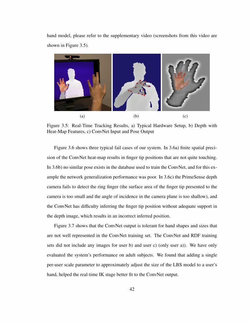
hand model, please refer to the supplementary video (screenshots from this video are

shown in Figure 3.5).

(a) (b) (c)

Figure 3.5: Real-Time Tracking Results, a) Typical Hardware Setup, b) Depth withHeat-Map Features, c) ConvNet Input and Pose Output

Figure 3.6 shows three typical fail cases of our system. In 3.6a) finite spatial preci-

sion of the ConvNet heat-map results in finger tip positions that are not quite touching.

In 3.6b) no similar pose exists in the database used to train the ConvNet, and for this ex-

ample the network generalization performance was poor. In 3.6c) the PrimeSense depth

camera fails to detect the ring finger (the surface area of the finger tip presented to the

camera is too small and the angle of incidence in the camera plane is too shallow), and

the ConvNet has difficulty inferring the finger tip position without adequate support in

the depth image, which results in an incorrect inferred position.

Figure 3.7 shows that the ConvNet output is tolerant for hand shapes and sizes that

are not well represented in the ConvNet training set. The ConvNet and RDF training

sets did not include any images for user b) and user c) (only user a)). We have only

evaluated the system’s performance on adult subjects. We found that adding a single

per-user scale parameter to approximately adjust the size of the LBS model to a user’s

hand, helped the real-time IK stage better fit to the ConvNet output.

42

a) b) c)

Figure 3.6: Fail Cases: RGB ground-truth (top row), inferred model [81] pose (bottomrow)

Comparison of the relative real-time performance of this work with relevant prior

art, such as that of [1] and [64], is difficult for a number of reasons. Firstly, [64] uses a

different capture device, which prevents fair comparison as it is impossible (without de-

grading sensor performance by using mirrors) for multiple devices to see the hand from

the same viewpoint simultaneously. Secondly, no third-party ground truth database of

poses with depth frames exists for human hands, so comparing the quantitative accuracy

of numerous methods against a known baseline is not possible. More importantly how-

ever, is that the technique utilized by [1] is optimized for an entirely different use case

and so fair comparison with their work is very difficult. [1] utilizes a vertically mounted

camera, can track multiple hands simultaneously, and is computationally less expensive

than the method presented in our work.

Figure 3.8 examines the performance of this work with the proprietary system of [1]

43

a) b) c)

Figure 3.7: Hand Shape/Size Tolerance: RGB ground-truth (top row), depth with anno-tated ConvNet output positions (bottom row)

(using the fixed-database version of the library), for 4 poses chosen to highlight the rel-

ative difference between the two techniques (images used with permission from 3Gear).

We captured this data by streaming the output of both systems simultaneously (using

the same RGBD camera). We mounted the camera vertically, as this is required for [1],

however our training set did not include any poses from this orientation. Therefore, we

expect our system to perform sub-optimally for this very different use case.

3.2 Future Work

As indicated in Figure 3.7, qualitatively we have found that the ConvNet general-

ization performance to varying hand shapes is acceptable but could be improved. We

are confident we can make improvements by adding more training data from users with

different hand sizes to the training set.

44

a) b) c) d)

Figure 3.8: Comparison with state-of-the-art commercial system: RGB ground-truth(top row), this work inferred model [81] pose (middle row), [1] inferred model pose(bottom row) (images used with permission from 3Gear).

For this work, only the ConvNet forward propagation stage was implemented on the

GPU. We are currently working on implementing the entire pipeline on the GPU, which

should improve performance of the other pipeline stages significantly. For example, the

GPU ConvNet implementation requires 5.6ms, while the same network executed on the

CPU (using optimized multi-threaded C++ code) requires 139ms.

The current implementation of our system can track two hands only if they are not

interacting. While we have determined that the dataset generation system can fit multiple

strongly interacting hand poses with sufficient accuracy, it is future work to evaluate the

45

neural network recognition performance on these poses. Likewise, we hope to evaluate

the recognition performance on hand poses involving interactions with non-hand objects

(such as pens and other man-made devices).

While the pose recovery implementation presented in this work is fast, we hope to

augment this stage by including a model-based fitting step that trades convergence ra-

dius for fit quality. Specifically, we suspect that replacing our final IK stage with an

energy-based local optimization method, inspired by the work of Li et al. [58] could

allow our method to recover second-order surface effects such as skin folding and skin-

muscle coupling from very limited data, and still with low-latency. In addition to in-

ference, such a localized energy-minimizing stage would enable improvements to the

underlying model itself. Since these localized methods typically require good registra-

tion, our method, which gives correspondence from a single image could advance the

state-of-the-art in non-rigid model capture.

Finally, we hope to augment our final IK stage with some form of temporal pose

prior to reduce jitter; for instance, using an extended Kalman filter as a post-processing

step to clean up the ConvNet feature output.

46

Part II

RGB-Based Localization of Human

Bodies

47

Chapter 4

Overview

4.1 Overview

In Part II (with extensions in Parts III and IV) we will address the problem of in-

ferring the 2D location of human joints in monocular RGB images - often called 2D

body-pose detection. Recent approaches to this problem fall into two broad categories:

1) more traditional deformable part models [79] and 2) deep-learning based discrimina-

tive models [97, 44, 43, 94, 95]. Bottom-up part-based models are a common choice for

this problem since the human body naturally segments into articulated parts. Tradition-

ally these approaches have relied on the aggregation of hand-crafted low-level features

such as SIFT [60] or HoG [20], which are then input to a standard classifier or a higher

level generative model. Care is taken to ensure that these engineered features are sensi-

tive to the part that they are trying to detect and are invariant to numerous deformations

in the input space (such as variations in lighting). On the other hand, discriminative

deep-learning approaches learn an empirical set of low and high-level features which are

typically more tolerant to variations in the training set and now outperform part-based

48

models. However, incorporating priors about the structure of the human body (such as

our prior knowledge about joint inter-connectivity) into such networks is difficult since

the low-level mechanics of these networks is often hard to interpret.

In this work we combine a ConvNet Part-Detector – which alone outperformed all

other existing methods at the time of publication [95] – with a part-based Spatial-Model

into a unified learning framework. An overview of this architecture is shown in Fig-

ure 4.1. In essence, this work is an attempt to combine the discriminative power of

deep-learning with the inter-joint connectivity priors enforced by the more traditional

deformable part models. In the first stage, we use a ConvNet to infer a probability dis-

tribution over spatial locations – or heat-map – describing the likelihood of each joint

occurring in that spatial location (in Figure 4.1 there are 14 ground truth joints and so the

ConvNet produces 14 heat-maps). The second stage graphical model inspired network

then “cleans up” the noisy heat-map outputs to enforce correct inter-joint consistency.

ConvNet

Part

Detector

GM to fix

mistakes

14 “noisy”

heat-maps

14 “clean”

heat-maps

Figure 4.1: Network architecture overview

Our translation-invariant ConvNet architecture utilizes a multi-resolution feature

representation with overlapping receptive fields. Additionally, our Spatial-Model is able

to approximate MRF loopy belief propagation, which is subsequently back-propagated

49

through, and learned using the same learning framework as the Part-Detector. We show

that the combination and joint training of these two models improves performance, and

allows us to significantly outperform existing state-of-the-art models on the task of hu-

man body pose recognition.

50

Chapter 5

Architecture

5.1 Model

5.1.1 Convolutional Network Part-Detector

Fully-Connected Layers

Image Patches

64x64

128x128

9x9x256LCN

64x64x3 30x30x128 13x13x128 9x9x128

LCN

64x64x3

512256

4

30x30x128 13x13x128 9x9x128

9x9x256

5x5 Conv + ReLU +

Pool

5x5 Conv + ReLU +

Pool

5x5 Conv + ReLU

Conv + ReLU + Pool (3 Stages)

LCN

Figure 5.1: Multi-Resolution Sliding-Window With Overlapping Receptive Fields

The first stage of our detection pipeline is a deep ConvNet architecture for body part

localization. The input is an RGB image containing one or more people and the output is

a heat-map, which produces a per-pixel likelihood for key joint locations on the human

skeleton.

51

A sliding-window ConvNet architecture is shown in Fig 5.1. The network is slid

over the input image to produce a dense heat-map output for each body-joint. Our

model incorporates a multi-resolution input with overlapping receptive fields. The upper

convolution bank in Fig 5.1 sees a standard 64x64 resolution input window, while the

lower bank sees a larger 128x128 input context down-sampled to 64x64. The input

images are then Local Contrast Normalized (LCN [18]) (after down-sampling with anti-

aliasing in the lower resolution bank) to produce an approximate Laplacian pyramid.

The advantage of using overlapping contexts is that it allows the network to see a larger

portion of the input image with only a moderate increase in the number of weights. The

role of the Laplacian Pyramid is to provide each bank with non-overlapping spectral

content which minimizes network redundancy.

Full Image 320x240px

Conv +

ReLU +Pool

(3 stages)

98x68x128 90x60x512 90x60x256 90x60x4

9x9 Conv + ReLU

1x1 Conv + ReLU

1x1 Conv + ReLU

Fully-connected equivalent model

Figure 5.2: Efficient Sliding Window Model with Single Receptive Field

An advantage of the Sliding-Window model (Fig 5.1) is that the detector is trans-

lation invariant. However a major drawback is that evaluation is expensive due to re-

dundant convolutions. Recent work [34, 82] has addressed this problem by performing

the convolution stages on the full input image to efficiently create dense feature maps.

These dense feature maps are then processed through convolution stages to replicate the

fully-connected network at each pixel. An equivalent but efficient version of the sliding

window model for a single resolution bank is shown in Fig 5.2. Note that due to pooling

in the convolution stages, the output heat-map will be a lower resolution than the input

52

image.

For our Part-Detector, we combine an efficient sliding window-based architecture

with multi-resolution and overlapping receptive fields; the subsequent model is shown

in Fig 5.3. Since the large context (low resolution) convolution bank requires a stride

of 1/2 pixels in the lower resolution image to produce the same dense output as the

sliding window model, the bank must process four down-sampled images, each with a

1/2 pixel offset, using shared weight convolutions. These four outputs, along with the

high resolution convolutional features, are processed through a 9x9 convolution stage

(with 512 output features) using the same weights as the first fully connected stage

(Fig 5.1) and then the outputs of the low resolution bank are added and interleaved with

the output of high resolution bank.

90x60x4Full Image 320x240px

98x68x128

Offset 4x160x120pximages

Conv +

ReLU +Pool

(3 stages)

Fully-connectioned equivalent model

Conv +

ReLU +Pool

(3 stages)

+53x38x128

Replicate + Offset + Stride 2

+ + +

(1, 1) (2, 1)(1, 2) (2, 2)

9x9 Conv + ReLU

...

...

90x60x512Interleaved

9x9 Conv + ReLU

9x9 Conv+ ReLU

9x9 Conv+ ReLU

Figure 5.3: Efficient Sliding Window Model with Overlapping Receptive Fields

To improve training time we simplify the above architecture by replacing the lower-

resolution stage with a single convolution bank as shown in Fig 5.4 and then upscale the

resulting feature map. In our practical implementation we use 3 resolution banks. Note

that the simplified architecture is no longer equivalent to the original sliding-window

network of Fig 5.1 since the lower resolution convolution features are effectively dec-

53

imated and replicated leading into the fully-connected stage, however we have found

empirically that the performance loss is minimal.

Full Image 320x240px

98x68x128

Half-res Image 160x120px

Conv +

ReLU +Pool

(3 stages)

Fully-connectioned equivalent model

90x60x512

Conv +

ReLU +Pool

(3 stages)

53x38x128

9x9 Conv + ReLU

45x30x12890x60x512

+Point-wiseUpscale

90x60x4

1x1 Conv+ ReLU

1x1 Conv+ ReLU

Figure 5.4: Approximation of Fig 5.3

Supervised training of the network is performed using batched Stochastic Gradient

Descent (SGD) with Nesterov Momentum. We use a Mean Squared Error (MSE) crite-

rion to minimize the distance between the predicted output and a target heat-map. The

target is a 2D Gaussian with a small variance and mean centered at the ground-truth joint

locations. At training time we also perform random perturbations of the input images

(randomly flipping and scaling the images) to increase generalization performance.

Note that an alternative model (such as in Tompson et al. [96]) would replace the

last 3 convolutional layers with a fully-connected neural network whose input context

is the feature activations for the entire input image. Such a model would be appropriate

if we knew a priori that there existed a strong correlation between skeletal pose and the

position of the person in the input frame since this alternative model is not invariant with

respect to the translation of the person within the image. However, the FLIC, LSP or

MPII datasets have no such strong pose-location bias (i.e. a subject’s torso is not always

in the same location in the image), and therefore a sliding-window based architecture is

more appropriate for our task.

54

5.1.2 Higher-Level Spatial-Model

(a) False Positive (b) Multiple Subjects

Figure 5.5: ConvNet Part Detector Fail Cases

The Part-Detector (Section 5.1.1) performance on our validation set predicts heat-

maps that contain many false positives and poses that are anatomically incorrect; for

instance when a peak for face detection is unusually far from a peak in the corresponding

shoulder detection. Figure 5.5a and 5.5b show two additional fail cases; when a strong

false positive outlier results in an incorrectly predicted joint location and when strong

activations from another subject result in the frame result in an incorrectly labeled joint.

Even in the presence of foreshortening, in both these cases it is clear that given the

length of the correctly labeled limbs, one should be able to improve the prediction given

that the incorrectly labeled limbs are anatomically incorrect.

In spite of the improved Part-Detector context (using our technique of overlapping

receptive fields), the feed forward network still has difficulty learning an implicit model

of the constraints of the body parts for the full range of body poses. We use a higher-level

Spatial-Model to constrain joint inter-connectivity and enforce global pose consistency.

The expectation of this stage is to not increase the performance of detections that are

55

already close to the ground-truth pose, but to remove false positive outliers that are

anatomically incorrect.

f

w e

s

e~e

s~sf

ww~

f~

sf ,

es,

we,

Figure 5.6: Linear chain MRF

Similar to Jain et al. [43], we formulate the Spatial-Model as an MRF model over the

distribution of spatial locations for each body part. The spatial model of [43] is shown

in Figure 5.6. f , s, e, w, f , s, e, and w are 2D random variables (or random Matrices),

describing the likelihood of the face, shoulder, elbow and wrist joints for each pixel

location in the input image 1. f , s, e and w are the noisy heat-maps from the ConvNet

output (Section 5.1.1) (or visible variables) and f , s, e, and w are the clean heat-maps

(or hidden variables) that we are trying to infer. Note that in practice, the full tree for

the LSP dataset will include 14 nodes and the tree for the FLIC dataset will include 7

nodes, one node for each of the joints we are trying to infer. For brevity only 4 nodes

are shown.

φ( f ), φ(s), φ(e) and φ(w) are the unary potentials (or sometimes called an image evi-

dence function when the factor between the hidden and visible variables is a 2D tensor),

and φ( f ), φ(s), φ(e) and ψ( f , s), ψ(s, e) and ψ(e,w) are the pair-wise factors describing

the joint priors between adjacent neighbors in the linear chain-MRF. As we will see,

1note that due to downsampling in the part detector this will be at a lower resolution than the input,and we use nearest-neighbor up-sampling to bring the heat-maps into the original resolution

56

these priors enforce inter-joint consistency. Using these factors, we can describe the

joint probability distribution as a product of factors, normalized by the partition func-

tion Z:

p(

f , s, e,w, f , s, e, w)

=1Z

∏i, j

ψ (xi)∏

k

φ (xk) (5.1)

The goal of our network is then to infer the distributions of the hidden variables

f , s, e and w by marginalization of other variables in the joint distribution. One such

method is to use a belief propagation formulation, which can be shown to converge to

an exact solution given that the MRF in Figure 5.6 is a tree-structured graph. After a

single round of belief propagation, the belief of a variable xi is given by the product of

incoming messages from each neighbor joint j, m ji (xi), multiplied by the unary factor

for the joint ψ (xi):

b (xi) = kφ (xi)∏j∈N(i)

m ji (xi) (5.2)

Here k is a normalizing partition function. Each incoming message from joint j to

joint i is described by the product of incoming messages to joint j from it’s neighbors

not including i (i.e. in the set N( j) − {i}, where N( j) is the set of adjacent neighbors

for node j), multiplied with the marginalized product of the unary potential for node j,

ψ(x j

), and the pair-wise factor between i and j, ψ

(x j, xi

):

m ji (xi)←∑

x j

φ(x j

)ψ

(x j, xi

) ∏k∈N( j)−{i}

mk j

(x j

)(5.3)

Since the height of our tree is 3, it can also be shown that message passing will

converge to the exact solution after 3 rounds. Writing out the full expression for the

57

marginalization of the hidden variable for the face joint we get:

b ( f ) = kφ( f )∑

s

φ(s)ψ(s, f )∑

e

φ(e)ψ(e, s)∑

w

φ(w)ψ(w, e) (5.4)

Note that we can also arrive at the same solution by marginalizing the joint distri-

bution of Equation 5.1, however the belief propagation formulation provides us with

invaluable insight as to the function of the pair-wise prior as we will show. Note that

the expression in Equation 5.4, requires sequential calculation of a 4D tensor and 2D

tensor products (for the multiplication of the pairwise and unary potentials), which is

then integrated over 2D to calculate the marginalized message distribution. To re-phrase

the above formation so that it is more amenable to implementation as a neural network,

we simplify Equation 5.4:

b ( f ) ≈ kφ( f )∏

i

∑xi

φ(xi)ψ(xi, f ) (5.5)

This means that rather than sequentially taking each product and multiplying before

marginalizing, the messages from adjacent joints can be calculated in parallel, which as

we shall see, is easier to implement as a single layer of neural network. However, by

doing so we have actually changed the structure of the MRF; the new formulation is a

star graph as shown in Figure 5.7 (visible nodes are not shown for brevity).

sf

e

w

s f

e

w

s

f

e

w

s

f

e

w

Figure 5.7: Star MRF

58

Note that Equation 5.5 is effectively a separate start graph for each of the joint

marginals that we will calculate, i.e. the marginalized hidden variable we infer for the

face joint, is not the same as the variable we use for the shoulder joint. Also not that we

have weakened our pair-wise priors; instead of modeling the tight coupling between the

shoulder and wrist, when incorporating evidence for marginalization of the face, instead

we will model the much looser pair-wise distribution of the wrist to face joint. Since

the average displacement between the face and wrist joint is large, the prior distribution

will not have high entropy and will therefore have a smaller impact on the marginalized

face distribution.

The 4D × 2D tensor product of the pairwise and unary factors as written in Equa-

tion 5.5 is extremely expensive to calculate. We therefore make one important approxi-

mation, instead of performing the tensor product then marginalizing, we instead replace

this with a convolution operator and use a ‘conditional pairwise’ factor as shown in

Equation 5.6. By doing so our implicit assumption is that the distribution of a joint‘s

location given the location of another joint is independent of the position in the input

image, i.e., the expected displacement between joints is the same and is independent of

the limb‘s position in the image. In our model this is a fair assumption for 2 reasons:

1) we expect that the movement of a joint is independent of the person‘s location in an

image and 2) we want to formulate a detector architecture that is translation invariant

and so modeling the full factor as a convolutional prior will achieve this.

b′ ( f ) ≈ kφ( f )∏

i

φ(xi) ∗ ψ(xi| f ) (5.6)

Note that this new formulation is no longer a traditional MRF, however it is still a

graphical model that is able to capture the inter-dependancies between joints. Lastly, we

add a scalar bias term, bxi | j, to each of the messages:

59

b′ ( f ) ≈ kφ( f )∏

i

φ(xi) ∗ ψ(xi| f ) + bxi | f (5.7)

This bias essentially sets a background probability distribution. This bias is ex-

tremely important since the ConvNet may output false negatives, particularly for diffi-

cult joints like the wrist and ankle, which results in a product with a zero probability,

causing strong positive activations for neighbor joints to be incorrectly attenuated. The

ratio between the dynamic range of the conditional prior and the strength of the bias

term sets how much a neighbor joint “trusts” the incoming message, and for strongly

coupled joints (like the face and shoulder), we indeed find that the network learns to set

the background bias close to zero during training. In contrast, for loosely coupled joints

(such as wrist and face), the network will learn to set the bias high and the dynamic

range of the prior term small.

Fig 5.8 shows a practical example of how the Spatial-Model is able to remove an

anatomically incorrect strong outlier from the face heat-map by incorporating the pres-

ence of a strong shoulder detection. For simplicity, only the shoulder and face joints are

shown, however, this example can be extended to incorporate all body part pairs. If the

shoulder heat-map shown in Fig 5.8 had an incorrect false-negative (i.e. no detection at

the correct shoulder location), the addition of the background bias bv→A would prevent

the output heat-map from having no maxima in the detected face region.

Fig 5.8 contains the conditional distributions for face and shoulder parts learned on

the FLIC [79] dataset. For any part xi the distribution ψ(xi, x j

)is the identity map,

and so the message passed from any joint to itself is its unary distribution. Since the

FLIC dataset is biased towards front-facing poses where the right shoulder is directly

to the lower right of the face, the model learns the correct spatial distribution between

these body parts and has high probability in the spatial locations describing the likely

60

x x

*

*

f|f

f|s

Face Unary

Shoulder Unary

Face

Shoulder

Face Unary

Shoulder Unary

*

*

s|f

s|s

=

=

=

=

Shoulder Face

Face Face Face Shoulder

Shoulder Shoulder

Figure 5.8: Didactic Example of Message Passing Between the Face and Shoulder Joints

displacement between the shoulder and face. For datasets that cover a larger range of the

possible poses (for instance the LSP [48] dataset), we would expect these distributions to

be less tightly constrained, and therefore this simple Spatial-Model will be less effective.

For our practical implementation we treat the distributions above as energies to avoid

the evaluation of k in Equation 5.7. There are 3 reasons why we do not include the par-

tition function. Firstly, we are only concerned with the maximum output value of our

network, and so we only need the output energy to be proportional to the normalized dis-

tribution. Secondly, since both the part detector and spatial model parameters contain

only shared weight (convolutional) parameters that are equal across pixel positions, eval-

uation of the partition function during back-propagation will only add a scalar constant

to the gradient weight, which would be equivalent to applying a per-batch learning-rate

modifier. Lastly, since the number of parts is not known a priori (since there can be

unlabeled people in the image), and since the distributions pv describe the part location

of a single person, we cannot normalize the Part-Model output. Our final model is a

modification to Eq 5.7:

61

eA = exp

∑v∈V

[log

(SoftPlus

(eA|v

)∗ ReLU (ev) + SoftPlus (bv→A)

)] (5.8)

where: SoftPlus (x) = 1/β log(1 + exp (βx)

), 1/2 ≤ β ≤ 2

ReLU (x) = max (x, ε) , 0 < ε ≤ 0.01

The network-based implementation of Eq 5.8 is shown in Fig 5.9. Eq 5.8 replaces the

outer multiplication of Eq 5.7 with a log space addition to improve numerical stability

and to prevent coupling of the convolution output gradients (the addition in log space

means that the partial derivative of the loss function with respect to the convolution

output is not dependent on the output of any other stages). However, this then requires

that our output criterion be before the outer exp, however for visualization the exp is

required. The inclusion of the SoftPlus and ReLU stages on the weights, biases and

input heat-map maintains a strictly greater than zero convolution output, which prevents

numerical issues for the values leading into the Log stage. Finally, a SoftPlus stage is

used to maintain continuous and non-zero weight and bias gradients during training.

With this modified formulation, Eq 5.8 is trained using back-propagation and SGD.

+

+

W11

Conv b

W

SoftPlusb11

SoftPluslog

W12

Conv b

W

SoftPlusb12

SoftPluslog

exp

exp

ReLU

ReLUW

21

Conv b

W

SoftPlusb21

SoftPluslog

W

SoftPlusb22

SoftPluslogConv

b

W22

Figure 5.9: Single Round Message Passing Network

The convolution sizes are adjusted so that the largest joint displacement is covered

62

within the convolution window. For our 90x60 pixel heat-map output, this results in

large 128x128 convolution kernels to account for a joint displacement radius of 64 pixels

(note that padding is added on the heat-map input to prevent pixel loss). Therefore

for such large kernels we use FFT convolutions based on the GPU implementation by

Mathieu et al. [62].

The convolution weights are initialized using the empirical histogram of joint dis-

placements created from the training examples. This initialization improves learned per-

formance, decreases training time and improves optimization stability. During training

we randomly flip and scale the heat-map inputs to improve generalization performance.

The FLIC and LSP datasets contain many frames with more than a single person,

while the joint locations from only one person in the scene are labeled. Therefore an

approximate torso bounding box is provided at test time for the single labeled person in

the scene. We incorporate this data by including an extra “torso-joint heat-map” to the

input of the Spatial-Model so that it can learn to select the correct feature activations in

a cluttered scene as shown in Figure 5.10.

Part-

Model

Spatial-

Model

Njnts

1

(Njnts+1)

torso heat-map:

Figure 5.10: Torso heat-map utilization

63

5.1.3 Unified Model

Since our Spatial-Model (Section 5.1.2) is trained using back-propagation, we can

combine our Part-Detector and Spatial-Model stages in a single Unified Model. To do so,

we first train the Part-Detector separately and store the heat-map outputs. We then use

these heat-maps to train a Spatial-Model. Finally, we combine the trained Part-Detector

and Spatial-Models and back-propagate through the entire network.

This unified fine-tuning further improves performance. We hypothesize that because

the Spatial-Model is able to effectively reduce the output dimension of possible heat-

map activations, the Part-Detector can use available learning capacity to better localize

the precise target activation.

64

Chapter 6


6.1 Results

The models from Sections 5.1.1 and 5.1.2 were implemented within the Torch7 [18]

framework (with custom GPU implementations for the non-standard stages above).

Training the Part-Detector takes approximately 48 hours, the Spatial-Model 12 hours,

and forward-propagation for a single image through both networks takes 51ms 1.

We evaluated our architecture on the FLIC [79] and extended-LSP [48] datasets.

These datasets consist of still RGB images with 2D ground-truth joint information gen-

erated using Amazon Mechanical Turk. The FLIC dataset is comprised of 5003 images

from Hollywood movies with actors in predominantly front-facing standing up poses

(with 1016 images used for testing), while the extended-LSP dataset contains a wider

variety of poses of athletes playing sport (10442 training and 1000 test images).

The FLIC-full dataset contains 20928 training images, however many of these train-

ing set images contain samples from the 1016 test set scenes and so would allow unfair

1We use a 12 CPU workstation with an NVIDIA Titan GPU

65

Figure 6.1: Sample images from FLIC-plus dataset

over-training on the FLIC test set. Therefore, we propose a new dataset - called FLIC-

plus (http://cims.nyu.edu/∼tompson/flic plus.htm) - which is a 17380 image subset from

the FLIC-plus dataset. Sample images from this dataset are shown in Figure 6.1. To cre-

ate this dataset, we produced unique scene labels for both the FLIC test set and FLIC-

plus training sets using Amazon Mechanical Turk. We then removed all images from

the FLIC-plus training set that shared a scene with the test set. Since 253 of the sample

images from the original 3987 FLIC training set came from the same scene as a test

set sample (and were therefore removed by the above procedure), we added these im-

ages back so that the FLIC-plus training set is a superset of the original FLIC training

set. Using this procedure we can guarantee that the additional samples in FLIC-plus are

sufficiently independent to the FLIC test set samples.

For evaluation of the test-set performance we use the measure suggested by Sapp et.

al. [79]. For a given normalized pixel radius (normalized by the torso height of each

sample) we count the number of images in the test-set for which the distance of the

predicted UV joint location to the ground-truth location falls within the given radius.

Fig 6.2a and 6.2b show our model’s performance on the the FLIC test-set for the el-

66

http://cims.nyu.edu/~tompson/flic_plus.htm

bow and wrist joints respectively and trained using both the FLIC and FLIC-plus training

sets. Performance on the LSP dataset is shown in Fig 6.2c and 6.3a. For LSP evaluation

we use person-centric (or non-observer-centric) coordinates for fair comparison with

prior work [97, 22]. Our model outperforms existing state-of-the-art techniques on both

of these challenging datasets with a considerable margin.

Ours (FLIC)

Ours (FLIC−plus)

Toshev et. al.

Jain et. al.

MODEC

Eichner et. al.

Yang et. al.

Sapp et. al.

0 2 4 6 8 10 12 14 16 18 200

10

20

30

40

50

60

70

80

90

100

Normalized distance error (pixels)

De

tectio

n r

ate

(a) FLIC: Elbow

0 2 4 6 8 10 12 14 16 18 200

10

20

30

40

50

60

70

80

90

100


De

tectio

n r

ate

(b) FLIC: Wrist

0 2 4 6 8 10 12 14 16 18 200

10

20

30

40

50

60

70

80

90

100


Dete

ction r

ate

Ours: wristOurs: elbowToshev et al.: wristToshev et al.: elbowDantone et al.: wristDantone et al.: elbowPishchulin et al.: wristPishchulin et al.: elbow

(c) LSP: Wrist and Elbow

Figure 6.2: Model Performance

Fig 6.3b illustrates the performance improvement from our simple Spatial-Model.

As expected the Spatial-Model has little impact on accuracy for low radii threshold,

however, for large radii it increases performance by 8 to 12%. Unified training of both

models (after independent pre-training) adds an additional 4-5% detection rate for large

radii thresholds.

The impact of the number of resolution banks is shown in Fig 6.3c). As expected, we

see a big improvement when multiple resolution banks are added. Also note that the size

of the receptive fields as well as the number and size of the pooling stages in the network

also have a large impact on the performance. We tune the network hyper-parameters

using coarse meta-optimization to obtain maximal validation set performance within

our computational budget (less than 100ms per forward-propagation).

67

0 2 4 6 8 10 12 14 16 18 200

10

20

30

40

50

60

70

80

90

100


De

tection r

ate

Ours: ankleOurs: kneeToshev et al.: ankleToshev et al.: kneeDantone et al.: ankleDantone et al.: kneePishchulin et al.: anklePishchulin et al.: knee

(a) LSP: Ankle and Knee

0 2 4 6 8 10 12 14 16 18 200

10

20

30

40

50

60

70

80

90

100


De

tection r

ate

Part−Model

Part and Spatial−Model

Joint Training

(b) FLIC: Wrist

0 2 4 6 8 10 12 14 16 18 200

10

20

30

40

50

60

70

80

90

100


De

tection r

ate

1 Bank

2 Banks

3 Banks

(c) FLIC: Wrist

Figure 6.3: (a) Model Performance (b) With and Without Spatial-Model (c) Part-Detector Performance Vs Number of Resolution Banks (FLIC subset)

Fig 6.4 shows the predicted joint locations for a variety of inputs in the FLIC and LSP

test-sets. Our network produces convincing results on the FLIC dataset (with low joint

position error), however, because our simple Spatial-Model is less effective for a number

of the highly articulated poses in the LSP dataset, our detector results in incorrect joint

predictions for some images. We believe that increasing the size of the training set will

improve performance for these difficult cases.

6.2 Multi-view Motion Capture

As an example of our detector used “in-the-wild”, Figure 6.6 shows results obtained

by using our detector‘s inferred heat-maps to improve an existing high-precision motion

capture system. This work was the result of a collaboration between NYU and MPII.

Our ConvNet model is used to estimate unary potentials for each joint of a kine-

matic skeleton model. These unary potentials are used to probabilistically extract pose

constraints for tracking by using weighted sampling from a pose posterior guided by

the model. In the final energy, these constraints are combined with an appearance-based

model-to-image similarity term. Poses can be computed very efficiently using iterative

68

Figure 6.4: Predicted Joint Positions, Top Row: FLIC Test-Set, Bottom Row: LSPTest-Set

local optimization, as ConvNet detection is fast, and our formulation yields a combined

pose estimation energy with analytic derivatives. In combination, this enables to track

full articulated joint angles at state-of-the-art accuracy and temporal stability with a very

low number of cameras. A very brief overview of the outline of this system is shown in

Figure 6.5. Since this work is as yet unpublished, we will refer interested readers to our

up-coming publication for more details.

69

Figure 6.5: Tracking results

Figure 6.6: Overview of the Tracking Architecture

70

Part III

Video-based Techniques for Improving

Performance

71

Chapter 7

Overview

7.1 Motion Features Overview

Traditional methods, as well as the architecture presented in Part II, typically use sin-

gle frame appearance cues such as texture patches, edges, color histograms, foreground

silhouettes or hand-crafted local features (such as histogram of gradients (HoG) [20]).

In Part III we will explore the use of motion-based features to improve performance

of our network architecture, and we will define and make use of many such features.

We will show that our results agree with psychophysical experiments [47], which have

shown that motion is a powerful visual cue that alone can be used to extract high-level

information, including articulated pose.

Previous work [31, 103] has reported that using motion features to aid pose infer-

ence has had little or no impact on performance. Simply adding high-order temporal

connectivity to traditional models would most often lead to intractable inference. In

Part III we show that deep learning is able to successfully incorporate motion features

and is able to out-perform existing state-of-the-art techniques. Further, we show that by

72

using motion features alone our method outperforms [27, 105, 80] (see Fig 6.2(a) and

(b)), which further strengthens our claim that information coded in motion features is

valuable and should be used when available.

We also present a new dataset called FLIC-motion, which is the FLIC dataset [79]

augmented with ‘motion-features’ for each of the 5003 images collected from Holly-

wood movies.

73

Chapter 8

Architecture

8.1 Body-Part Detection Model

We propose a simple extension to the model presented in Part II: Section 5.1.1;

the input to the network is an RGB image and an additional set of motion features.

Therefore, instead of the previous 3 channel input, the new model will now use 4 to

6 features depending on the motion feature used and we investigate a wide variety of

motion feature formulations (section 8.1.1). Finally, we will also introduce a simple

Spatial-Model to solve a specific sub-problem associated with evaluation of our model

on the FLIC-motion dataset (section 8.1.3). For Part III, we will use the full graphical

model described in Part II: Section 5.1.2, but rather we will implement a simplified

model in order to better highlight the impact of our chosen motion features.

8.1.1 Motion Features

Psychophysical experiments [47], have shown that motion is very a powerful visual

cue for extracting high-level information. In these experiments, the main joints of a

74

human were represented as a single point, thus degrading the appearance of the object

to a minimum, ensuring that any recognition must be based solely on motion. They

concluded that proximal motion patterns give the human visual system highly efficient

information that carry all the essential information needed for immediate visual identi-

fication of such human motions.

The aim of this section is to incorporate features that are representative of the true

motion-field (the perspective projection of the 3D velocity-field of moving surfaces) as

input to our detection network so that it can exploit motion as a cue for body part local-

ization. To this end, we evaluate and analyze four motion features which fall under two

broad categories: those using simple derivatives of the RGB video frames and those us-

ing optical flow features. For each RGB image pair fi and fi+δ, we propose the following

features:

• RGB image pair - { fi, fi+δ}

• RGB image and an RGB difference image - { fi, fi+δ − fi}

• Optical-flow1 vectors - { fi,FLOW( fi, fi+δ)}

• Optical-flow magnitude - { fi, ||FLOW( fi, fi+δ)||2}

The RGB image pair is by far the simplest way of incorporating the relative mo-

tion information between the two frames. However, this representation clearly suffers

from a lot of redundancy (i.e. if there is no camera movement) and is extremely high

dimensional. Furthermore, it is not obvious to the deep network what changes in this

high dimensional input space are relevant temporal information and what changes are

due to noise or camera motion. A simple modification to this representation is to use a

1We use the algorithm proposed by Weinzaepfel et al. [101] to compute optical-flow.

75

difference image, which reformulates the RGB input so that the algorithm sees directly

the pixel locations where high energy corresponds to motion (alternatively the network

would have to do this implicitly on the image pair). A more sophisticated representa-

tion is optical-flow, which is considered to be a high-quality approximation of the true

motion-field. Implicitly learning to infer optical-flow from the raw RGB input would

be non-trivial for the network to estimate, so we perform optical-flow calculation as a

pre-processing step (at the cost of greater computational complexity).

8.1.1.1 FLIC-motion dataset:

We propose a new dataset which we call FLIC-motion2. It is comprised of the orig-

inal FLIC dataset of 5003 labeled RGB images collected from 30 Hollywood movies,

of which 1016 images are held out as a test set, augmented with the aforementioned

motion features.

We experimented with different values for δ and investigated the above features with

and without camera motion compensation; we use a simple 2D projective motion model

between fi and fi+δ, and warp fi+δ onto fi using the inverse of this best fitting projection

to approximately remove camera motion. A comparison between image pairs with and

without warping can be seen in Fig 8.1.

To obtain fi+δ, we must know where the frames fi occur in each movie. Unfortu-

nately, this was non-trivial as the authors Sapp et al. [79] could not provide us with the

exact version of the movie that was used for creating the original dataset. Corresponding

frames can be very different in multiple versions of the same movie (4:3 vs wide-screen,

director’s cut, special editions, etc.). We estimate the best similarity transform S be-

tween fi and each frame f mj from the movie m, and if the distance | fi − S f m

j | is below

2This dataset can be downloaded from http://cs.nyu.edu/˜ajain/accv2014/

76

http://cs.nyu.edu/~ajain/accv2014/

(a)

20

15

10

5

(b) (c) (d)

Figure 8.1: Results of optical-flow computation: (a) average of frame pair, (b) opticalflow on (a), (c) average of frame pair after camera compensation, and (d) optical-flowon (c)

a certain threshold (10 pixels), we conclude that we found the correct frame. We visu-

ally confirm the resulting matches and manually pick frames for which the automatic

matching was unsuccessful (e.g. when enough feature points were not found).

8.1.2 Convolutional Network

As previously mentioned, the network architecture is a simple extension to the net-

work described in Section 5.1.1. The sliding window model of the new network is

shown in Figure 8.2, with the additional motion feature inputs. Another slight variation

to the model of Section 5.1.1 is that not only are the input patches first normalized using

Local Contrast Normalization (LCN [18]) for the RGB channels, we also normalize the

motion features with a new normalization method we call Local Motion Normalization

(LMN). We formulate LMN as the local subtraction with the response from a Gaussian

kernel with large standard deviation followed by a divisive normalization. The result is

that it removes some unwanted background camera motion as well as normalizing the

local intensity of motion (which helps improve network generalization for motions of

varying velocity but with similar pose). Note that the result of this stage is similar to the

technique of Matsushita et al. [63], who also use Gaussian high-pass filtering on motion

77

flow images to remove undesired camera motion when performing camera stabilization.

Prior to processing through the convolution stages, the normalized motion channels are

concatenated along the feature dimension with the normalized RGB channels, and the

resulting tensor is processed though the same efficient sliding window network architec-

ture as was presented in Section 5.1.1 and will not be replicated here for brevity.

5x5 Conv+ ReLU+ Pool

30

30

163 + nf

Image Patches

Flow Patches

64

64

3

13

13

16

5x5 Conv+ ReLU+ Pool

64

64

99

16

1296

512

256

4

5x5 Conv+ ReLU

nf

Conv + ReLU + Pool (3x)

64

64

LCN

LMN

Motion Feature Patches

...

...

...

...

Figure 8.2: Sliding-window with image and flow patches

8.1.3 Simple Spatial Model

Instead of using the spatial model from Section 5.1.2, we will use a simplified model

for the experiments in Section 9 to better highlight the impact of our chosen motion

features. When the full model is used, the performance on the FLIC dataset is so high

that the included motion features will have a marginal contribution to performance. We

believe that on harder datasets (such as LSP and MPII) this impact will be greater,

however at the time of writing we do not have access to multiple video frames for these

datasets.

The core of our simplified Spatial-Model is an empirically calculated joint-mask,

shown in Fig 8.3(b). The joint-mask layer describes the possible joint locations, given

78

that the supplied torso position is in the center of the mask. To create a mask layer for

body part A, we first calculate the empirical histogram of the part A location, xA, relative

to the torso position xT for the training set examples; i.e. xhist = xA − xT . We then turn

this histogram into a Boolean mask by setting the mask amplitude to 1 for pixels for

which p (xhist) > 0. Finally, we blur the mask using a wide Gaussian low-pass filter

which accounts for body part locations not represented in the training set (but which

might be present in the test set).

x =

(a) (b) (c)

Figure 8.3: Simple spatial model used to mask-out the incorrect shoulder activationsgiven a 2D torso position

The inclusion of this stage has two major advantages. Firstly, as with the full graphi-

cal model from Section 5.1.2 the correct feature activation from the Part-Detector output

is selected for the person for whom a ground-truth label was annotated. An example of

this is shown in Fig 8.3. Secondly, since the joint locations of each part are constrained

in proximity to the single ground-truth torso location, then (indirectly) the connectivity

between joints is also constrained, enforcing that inferred poses are anatomically viable

(i.e. the elbow joint and the shoulder joint cannot be to far away from the torso, which

in turn enforces spatial locality between the elbow and shoulder joints).

During test time, this joint-mask is shifted to the ground-truth torso location and the

per-pixel energy from the Part-Model (section 8.1.2) is then multiplied with the mask to

79

produce a filtered output. This process is carried out for each body part independently.

One can view this simplified model as a star graph with the torso joint as the root and

all joints as children to the torso. With weaker prior terms In comparison to the full

spatial model from Section 5.1.2 (since the torso is only weakly coupled to joints such

as the wrist and ankle), we do not expect this model to work as well but it will help

disambiguate when there are multiple subjects per frame.

It should be noted that while this Spatial-Model does enforce some anatomic consis-

tency, it does have limitations. Notably, we expect it to fail for datasets where the range

of poses is not as constrained as the FLIC dataset (which is primarily front facing and

standing up poses).

80

Chapter 9


9.1 Results

Training time on the FLIC-motion dataset (3957 training set images, 1016 test set

images) for the model of Section 8.1.2 is similar to the original model in Section 5;

approximately 12 hours. FPROP of a single image takes approximately 50ms1. For our

models that use optical flow as a motion feature input, the most expensive part of our

pipeline is the optical flow calculation, which takes approximately 1.89s per image pair.

We plan to investigate real-time flow estimations in the future.

Section 9.1.1 compares the performance of the motion features from section 8.1.1.

Section 9.1.2 compares our architecture with other techniques and shows that our system

significantly outperforms existing state-of-the-art techniques. Note that for all experi-

ments in Section 9.1.1 we use a smaller model with 16 convolutional features in the first

3 layers. A model with 128 instead of 16 features for the first 3 convolutional layers is

used for results in Section 9.1.2.1Analysis of our system was on a 12 core workstation with an NVIDIA Titan GPU

81

9.1.1 Comparison and Analysis of Proposed Motion Features

Fig 9.1 shows a selection of example images from the FLIC test set which highlights

the importance of using motion features for body pose detection. In Fig 9.1(a), the elbow

position is occluded by the actor’s sling, and no such examples exist in the training

set; however, the presence of body motion provides a strong cue for elbow location.

Figs 9.1(b) and (d) have extremely cluttered backgrounds and the correct joint location

is locally similar to the surrounding region (especially for the camouflaged clothing in

Fig 9.1(d)). For these images, motion features are essential in correct joint localization.

Finally, Fig 9.1(c) is an example where motion blur (due to fast joint motion) reduces

the fidelity of RGB edge features, which results in incorrect localization when motion

features are not used.

Figure 9.1: Predicted joint positions on the FLIC test-set. Top row: detection withmotion features (L2 motion flow). Bottom row: without motion features (baseline).

Figs 9.2(a) and (b) show the performance of the motion features of section 8.1.1 on

the FLIC-motion dataset for the elbow and wrist joints respectively. As per the evalua-

tion of Section 6, we again use the criterion proposed by Sapp et al. [79]. Surprisingly,

82

even the simple frame-difference temporal feature improves upon the baseline result

(which we define as a single RGB frame input – i.e. the model from Section 8.1.2) and

even outperforms the 2D optical flow input (see 9.1(b) inset).

0 2 4 6 8 10 12 14 16 18 200

20

40

60

80

100

Distance Threshold (pixels)

De

tectio

n R

ate

(p

erc

en

t)

BaselineMotion Flow Magnitude2D Motion FlowImage PairDifference Image

(a)

0 2 4 6 8 10 12 14 16 18 200

10

20

30

40

50

60

70

80


Dete

ction R

ate

(perc

ent)

BaselineMotion Flow Magnitude2D Motion FlowImage PairDifference Image

10 12 14

60

65

70

(b)

Figure 9.2: Model performance for various motion features

Note that stable and accurate calculation of optical-flow from arbitrary RGB videos

is a very challenging problem. Therefore, incorporating motion flow features as input

to the network adds non-trivial localization cues that would be very difficult for the

network to learn internally with limited learning capacity. Therefore, it is expected that

the best performing networks in Fig 9.2 are those that incorporate motion flow features.

However, it is surprising that using the magnitude of the flow vectors performs as well

as – and in some cases outperforms – the full 2D motion flow. Even though the input

data is richer, we hypothesize that when using 2D flow vectors the network must learn

invariance to the direction of joint movement; for instance, the network should predict

the same head position whether a person is turning his/her head to the left or right on

the next frame. On the other hand, when the L2 magnitude of the flow vector is used,

the network sees the high velocity motion cue but cannot over-train to the direction of

83

the movement.

Fig 9.3(a) shows that the performance of our network is relatively agnostic to the

frame separation (δ) between the samples for which we calculate motion flow; the av-

erage precision between 0 and 20 pixel radii degrades 3.9% from -10 pixels offset to -1

pixel offset. A frame difference of 10 corresponds to approximately 0.42sec (at 24fps),

and so we expect that large motions over this time period would result in complex non-

linear trajectories in input space for which a single finite difference approximation of

the pixel velocity would be inaccurate. Accordingly, our results show that performance

indeed degrades as a larger frame step is used.

−10 −8 −6 −4 −2 0 2 4 6 8 100.52

0.53

0.54

0.55

0.56

0.57

0.58

Frame Step Size for Optical Flow

Ave

rag

e P

recis

ion

(p

erc

en

t)

baseline

(a)

0 2 4 6 8 10 12 14 16 18 200

20

40

60

80

100


Dete

ction R

ate

(perc

ent)

Without Camera Correction

With Camera Correction

(b)

Figure 9.3: Model performance for (a) varying motion feature frame offsets (b) with andwithout camera motion compensation

Similarly, we were surprised that our camera motion compensation technique (de-

scribed in section 8.1.1) does not help to the extent that we expected, as shown in

Fig 9.3(b). Likely this is because either LMN removes a lot of constant background

motion or the network is able to learn to ignore the remaining foreground-background

parallax motion due to camera movement.

84

9.1.2 Comparison with Other Techniques

Fig 9.4(a) and 9.4(b) compares the performance of the Section 8.1.2 model with

other state-of-the-art models on the FLIC dataset for the elbow and wrist joints respec-

tively. Our detector is able to significantly outperform all prior techniques on this chal-

lenging dataset. However, this result is not surprising since the baseline model from

Section 5 also outperforms state-of-the-art.

Ours

Only Flow Mag.

Toshev et. al.

Jain et. al.

MODEC

Eichner et. al.

Yang et. al.

Sapp et. al.

0 2 4 6 8 10 12 14 16 18 200

20

40

60

80

100


Dete

ction R

ate

(perc

ent)

(a)

0 2 4 6 8 10 12 14 16 18 200

20

40

60

80

100


Dete

ction R

ate

(perc

ent)

(b)

Figure 9.4: Our model performance compared with our model using only flow magni-tude features (no RGB image), Toshev et al. [97], Jain et al. [43], MODEC [79], Eichneret al. [27], Yang et al. [105] and Sapp et al. [80].

Note that using only motion features already outperforms [27, 105, 80]. Also note

that using only motion features is less accurate than using a combination of motion

features and RGB images, especially in the high accuracy region. This is because fine

details such as eyes and noses are missing in motion features. Increasing the complexity

of our simple spatial model by using the full model from Section 5.1.2 will improve

performance further, specifically for large radii offsets.

85

Part IV

Efficient Localization in the Presence of

Pooling

86

Chapter 10

Overview

10.1 Motivation and Pooling Overview

A common characteristic of recent ConvNet architectures used for human body pose

detection [95, 44, 97, 16] to date, including the architectures presented in Parts I, II and

III, is that they make use of internal strided-pooling layers. These layers reduce the

spatial resolution by computing a summary statistic over a local spatial region (typi-

cally a max operation in the case of the commonly used Max-Pooling layer). The main

motivation behind the use of these layers is to promote invariance to local input trans-

formations (particularly translations) since their outputs are invariant to spatial location

within the pooling region. This is particularly important for image classification where

local image transformations obfuscate object identity. Therefore pooling plays a vital

role in preventing over-training while reducing computational complexity for classifica-

tion tasks.

As we will show in Section 12, the spatial invariance achieved by pooling layers

comes at the price of limiting spatial localization accuracy. As such, by adjusting the

87

amount of pooling in the network, for localization tasks a trade-off is made between

generalization performance, model size and spatial accuracy.

In Part IV we present a ConvNet architecture for efficient localization of human

skeletal joints in monocular RGB images that achieves high spatial accuracy without

significant computational overhead. This model allows us to use increased amounts of

pooling for computational efficiency, while retaining high spatial precision.

We begin by presenting a ConvNet architecture to perform coarse body part local-

ization that is based off the model presented in Section 5. This network outputs a low

resolution, per-pixel heat-map, describing the likelihood of a joint occurring in each

spatial location. We use this architecture as a platform to discuss and empirically eval-

uate the role of Max-pooling layers in convolutional architectures for dimensionality

reduction and improving invariance to noise and local image transformations. We then

present a novel network architecture that reuses hidden-layer convolution features from

the coarse heat-map regression model in order to improve localization accuracy. By

jointly-training these models, we show that our model outperforms recent state-of-the-

art on standard human body pose datasets [5, 79].

88

Chapter 11

Architecture

11.1 Coarse Heat-Map Regression Model

For the experimental results of Part IV, we use the multi-resolution ConvNet archi-

tecture shown in Figure 11.1 on the FLIC [79] dataset, and a similarly structured, albeit

deeper and wider, ConvNet model for the MPII [5] dataset. Both these models are an

extension of the model from Section 5. For brevity, in Section 11.1.1 we will only dis-

cuss the relevant extensions and refer readers to Section 5 for more details regarding the

higher-level network architecture.

11.1.1 Model Architecture

The network architecture of Figure 11.1 includes more features per convolution layer

and more layers than the architecture from Section 5. This is possible for 2 reasons.

Firstly, the Convolution and ReLU layers are implemented as a single layer, which

significantly reduces the GPU memory required to FPROP and BPROP the network.

This is possible because the output of the convolution layer is not needed when back-

89

LCN +

5x5 Conv+

ReLU +

2x2 MaxPool

3x256x256 128x128x128

5x5 Conv+

ReLU +

2x2 MaxPool

128x64x64 128x32x32

9x9 Conv+

ReLU

512x32x32

LCN +

5x5 Conv+

ReLU +

2x2 MaxPool

128x64x64

5x5 Conv+

ReLU +

2x2 MaxPool

128x32x32

5x5 Conv+

ReLU +

2x2 MaxPool

128x16x16

9x9 Conv+

ReLU

512x16x16 3x128x128

2x2 Upscale

512x32x32

+

512x32x32

1x1 Conv+

ReLU

256x32x32

1x1 Conv+

ReLU

256x32x32

1x1 Conv+

ReLU

14x32x32

Heat-Maps

SpatialDropout

5x5 Conv+

ReLU +

2x2 MaxPool

Figure 11.1: Multi-resolution Sliding Window Detector With Overlapping Contexts(model used on FLIC dataset)

propagating the output derivative through the ReLU layer; the output derivative is simply

‘zeroed’ for the pixel locations for which the output of the ReLU is zero and this zeroed

derivative map is then back-propagated through the convolution layer. Therefore, we can

use temporary memory for storing the intermediate output and gradient which reduces

overall memory usage. Secondly, we have added a new regularization mechanism, Spa-

tialDropout (discussed in Section 11.1.2), which allows us to add more features (thus

increasing learning capacity and performance) without over-training.

We use an input resolution of 320x240 and 256x256 pixels for the FLIC [79] and

MPII [5] datasets respectively.

11.1.2 SpatialDropout

As mentioned above, we improve upon the model of Section 5 ([95]), by adding

an additional dropout layer before the first 1x1 convolution layer in Figure 11.1. The

role of dropout is to improve generalization performance by preventing activations from

becoming strongly correlated [39], which in turn leads to over-training. In the standard

dropout implementation, network activations are “dropped-out” (by zeroing the activa-

tion for that neuron) during training with independent probability pdrop. At test time all

90

activations are used, but a gain of 1 − pdrop is multiplied to the neuron activations to

account for the increase in expected bias.

In initial experiments, we found that applying standard dropout (where each convo-

lution feature map activation is “dropped-out” independently) before the 1 × 1 convolu-

tion layer generally increased training time but did not prevent over-training. Since our

network is fully convolutional and natural images exhibit strong spatial correlation, the

feature map activations are also strongly correlated, and in this setting standard dropout

fails.

F2 F1

W2Pos1

W2Pos2

W1Pos1

W1Pos2

f2a f2b f1a f1b ( = dropped-out)

de/df1b de/df1a de/df2b de/df2a

Figure 11.2: Standard Dropout after a 1D convolution layer

Standard dropout at the output of a 1D convolution is illustrated in Figure 11.2.

The top two rows of pixels represent the convolution kernels for feature maps 1 and 2,

and the bottom row represents the output features of the previous layer. During back-

propagation, the center pixel of the W2 kernel receives gradient contributions from both

f2a and f2b as the convolution kernel W2 is translated over the input feature F2. In this

example f2b was randomly dropped out (so the activation was set to zero) while f2a was

not. Since F2 and F1 are the output of a convolution layer we expect f2a and f2b to

be strongly correlated: i.e. f2a ≈ f2b and de/d f2a ≈ de/d f2b (where e is the error function

to minimize). While the gradient contribution from f2b is zero, the strongly correlated

f2a gradient remains. In essence, the effective learning rate is scaled by the dropout

91

probability p, but independence is not enhanced.

Instead we formulate a new dropout method which we call SpatialDropout. For a

given convolution feature tensor of size nfeats × height × width, we perform only nfeats

dropout trials and extend the dropout value across the entire feature map. Therefore,

adjacent pixels in the dropped-out feature map are either all 0 (dropped-out) or all ac-

tive as illustrated in Figure 11.3. We have found this modified dropout implementation

improves performance, especially on the FLIC dataset, where the training set size is

small.

F2 F1

W2Pos1

W2Pos2

W1Pos1

W1Pos2

f2a f2b f1a f1b

de/df1b de/df1a de/df2b de/df2a

( = dropped-out)

Figure 11.3: SpatialDropout after a 1D convolution layer

11.1.3 Training and Data Augmentation

We train the model in Figure 11.1 by minimizing the Mean-Squared-Error (MSE)

distance of our predicted heat-map to a target heat-map. The target is a 2D Gaussian of

constant variance (σ ≈ 1.5 pixels) centered at the ground-truth (x, y) joint location. The

objective function is:

E1 =1N

N∑j=1

∑xy

∥∥∥H′j (x, y) − H j (x, y)∥∥∥2

(11.1)

Where H′j and H j are the predicted and ground truth heat-maps respectively for the

92

jth joint.

During training, each input image is randomly rotated (r ∈ [−20◦,+20◦]), scaled

(s ∈ [0.5, 1.5]) and flipped (with probability 0.5) in order to improve generalization per-

formance on the validation-set. Additionally we use the spatial model from Section 5.1.2

([95]) to discriminate between multiple people in each frame using the approximate

torso position supplied at test time for the FLIC and MPII datasets.

11.2 Fine Heat-Map Regression Model

In essence, the goal of Part IV is to recover the spatial accuracy lost due to pooling

of the model in Part II by using an additional ConvNet to refine the localization result

of the coarse heat-map. However, unlike a standard cascade of models, as in the work

of Toshev et al. [97], we reuse existing convolution features. This not only reduces

the number of trainable parameters in the cascade, but also acts as a regularizer for the

coarse heat-map model since the coarse and fine models are trained jointly.

11.2.1 Model Architecture

The full system architecture is shown in Figure 11.4. It consists of the heat-map-

based parts model from Section 11.1.1 for coarse localization, a module to sample and

crop the convolution features at a specified (x, y) location for each joint, as well as an

additional convolutional model for fine tuning.

Joint inference from an input image is as follows: we forward-propagate (FPROP)

through the coarse heat-map model then infer all joint (x, y) locations from the maximal

value in each joint’s heat-map. We then use this coarse (x, y) location to sample and crop

the first 2 convolution layers (for all resolution banks) at each of the joint locations. We

93

128x256x256

128x128x128

128x128x128

128x64x64

Coarse Heat-Map Model

conv

conv

3x conv

pool conv pool 2xconv+

pool

pool conv pool 2xconv+

pool

Crop

at

(x,y) 14x128x36x36

14x128x18x18

14x128x18x18

14x128x9x9

3x256x256

14x32x32

coarse (x,y)

Fine Heat-

Map Model

lcn

lcn

Final (x,y)

14x36x36 (¢x, ¢y)

refinement

Figure 11.4: Overview of our Cascaded Architecture

then FPROP these features through a fine heat-map model to produce a (∆x,∆y) offset

within the cropped sub-window. Finally, we add the position refinement to the coarse

location to produce a final (x, y) localization for each joint.

Figure 11.5 shows the crop module functionality for a single joint. We simply crop

out a window centered at the coarse joint (x, y) location in each resolution feature map,

however we do so by keeping the contextual size of the window constant by scaling

the cropped area at each higher resolution level. Note that back-propagation (BPROP)

through this module from output feature to input feature is trivial; output gradients from

the cropped image are simply added to the output gradients of the convolution stages in

the coarse heat-map model at the sampled pixel locations.

256x256

9x9

18x18

36x36 (x,y)

128x128

64x64

Figure 11.5: Crop module functionality for a single joint

The fine heat-map model is a Siamese network [13] of 7 instances (14 for the MPII

dataset), where the weights and biases of each module are shared (i.e. replicated across

94

all instances and updated together during BPROP). Since the sample location for each

joint is different, the convolution features do not share the same spatial context and so

the convolutional sub-networks must be applied to each joint independently. However,

we use parameter sharing amongst each of the 7 instances to substantially reduce the

number of shared parameters and to prevent over-training. At the output of each of the

7 sub-networks we then perform a 1x1 Convolution, with no weight sharing to output a

detailed-resolution heat-map for each joint. The purpose of this last layer is to perform

the final detection for each joint.

14x128x36x36 14x128x18x18 14x128x18x18

14x128x9x9

Face Instance

1x1 Conv+

ReLU 36x36

Lsho Instance

Lelb Instance

14 joints

total

Shared weights/biases

Figure 11.6: Fine heat-map model: 14 joint Siamese network

Note we are potentially performing redundant computations in the Siamese network.

If two cropped sub-windows overlap and since the convolutional weights are shared, the

same convolution maybe applied multiple times to the same spatial locations. However,

we have found in practice this is rare. Joints are infrequently co-located, and the spatial

context size is chosen such that there is little overlap between cropped sub-regions (note

that the context of the cropped images shown in Figures 11.4 and 11.7 are exaggerated

for clarity).

95

Each instance of the sub-network in Figure 11.6 is a ConvNet of 4 layers, as shown in

Figure 11.7. Since the input images are different resolutions and originate from varying

depths in the coarse heat-map model, we treat the input features as separate resolution

banks and apply a similar architecture strategy as used in Section 11.1.1. That is we

apply the same size convolutions to each bank, upscale the lower-resolution features to

bring them into canonical resolution, add the activations across feature maps then apply

1x1 convolutions to the output features.

64x36x36

7x7 Conv+

ReLU

64x36x36

9x9 Conv+

ReLU

128x36x36

64x18x18 64x18x18 128x18x18 128x36x36

128x36x36

2x2 Upscale

+

128x36x36

1x1 Conv+

ReLU

128x36x36

5x5 Conv+

ReLU

64x18x18 64x18x18 128x18x18 128x36x36

64x9x9 64x9x9 128x9x9 128x36x36 4x4 Upscale

128x18x18

128x18x18

128x9x9

Figure 11.7: The fine heat-map network for a single joint

It should be noted that this cascaded architecture can be extended further as is possi-

ble to have multiple cascade levels each with less and less pooling. However, in practice

we have found that a single layer provides sufficient accuracy, and in particular within

the level of label noise on the FLIC dataset (as we show in Section 12.1).

96

11.2.2 Joint Training

We jointly train both the coarse and fine heat-map models together by minimizing

the following objective function:

E2 = E1 + λ1N

N∑j=1

∑x,y

∥∥∥G′j (x, y) −G j (x, y)∥∥∥2

(11.2)

Where G′ and G are the set of predicted and ground truth heat-maps respectively

for the fine heat-map model, λ is a constant used to trade-off the relative importance of

both sub-tasks and E1 is the coarse heat-map model contribution from Equation 11.1.

We treat λ as another network hyper-parameter and is chosen to optimize performance

over our validation set (we use λ = 0.1). Ideally, a more direct optimization function

would attempt to measure the argmax of both heat-maps and therefore directly minimize

the final (x, y) prediction. However, since the argmax function is not differentiable we

instead reformulate the problem as a regression to a set of target heat-maps and minimize

the distance to those heat-maps.

97

Chapter 12


12.1 Results

The ConvNet architecture for Part IV was again implemented within the Torch7 [18]

framework and evaluation is performed on the FLIC [79] and MPII-Human-Pose [5]

datasets. Since the FLIC poses are predominantly front-facing and upright, FLIC is

considered to be less challenging. However the small number of training examples

makes the dataset a good indicator for generalization performance, which is a evaluation

test for our SpatialDropout layer. On the other-hand the MPII dataset is very challenging

and it includes a wide variety of full-body pose annotations within the 28,821 training

and 11,701 test examples. For evaluation of our model on the FLIC dataset we use again

the standard PCK [79] measure used in Parts II and III and we use the PCKh measure

of [5] for evaluation on the MPII dataset.

Figure 12.1 shows the PCK test-set performance of our coarse heat-map model (Sec-

tion 11.1.1) when various amounts of pooling are used within the network (keeping the

number of convolution features constant). Figure 12.1 results show quite clearly the

98

expected effect of coarse quantization in (x, y) and therefore the impact of pooling on

spatial precision; when more pooling is used the performance of detections within small

distance thresholds is reduced.

0 0.05 0.1 0.15 0.20

10

20

30

40

50

60

70

80

90

100

Normalized distance

De

tectio

n r

ate

, %

4x pool

8x pool

16x pool

Figure 12.1: Pooling impact on FLIC test-set Average Joint Accuracy for the coarseheat-map model

For joints where the ground-truth label is ambiguous and difficult for the human

mechanical-turkers to label, we do not expect our cascaded network to do better than

the expected variance in the user-generated labels. To measure this variance (and thus

estimate the upper bound of performance) we performed the following informal experi-

ment: we showed 13 users 10 random images from the FLIC training set with annotated

ground-truth labels as a reference so that the users could familiarize themselves with

the desired anatomical location of each joint. The users then annotated a consistent set

of 10 random images from the FLIC test-set for the face, left-wrist, left-shoulder and

left-elbow joints. Figure 12.2 shows the resultant joint annotations for 2 of the images.

To estimate joint annotation noise we calculate the standard deviation (σ) across

user annotations in x for each of the 10 images separately and then average the σ across

99

Figure 12.2: User generated joint annotations

the 10 sample images to obtain an aggregate σ for each joint. Since we down-sample

the FLIC images by a factor of 2 for use with our model we divide the σ values by the

same down-sample ratio. The result is shown in Table 12.1:

Face Shoulder Elbow Wrist

Label Noise (10 images) 0.65 2.46 2.14 1.57This work 4x (test-set) 1.09 2.43 2.59 2.82This work 8x (test-set) 1.46 2.72 2.49 3.41This work 16x (test-set) 1.45 2.78 3.78 4.16

Table 12.1: σ of (x, y) pixel annotations on FLIC test-set images (at 360×240 resolution)

The histogram of the coarse heat-map model pixel error (in the x dimension) on

the FLIC test-set when using an 8x internal pooling is shown in Figure 12.3a (for the

face and shoulder joints). For demonstration purposes, we quote the error in the pixel

coordinates of the input image to the network (which for FLIC is 360 × 240), not the

original resolution. As expected, in these coordinates there is an approximately uniform

uncertainty due to quantization of the heat-map within -4 to +4 pixels. In contrast to

this, the histogram of the cascaded network is shown in Figure 12.3b and is close to the

100

measured label noise1.

−10−8 −6 −4 −2 0 2 4 6 8 100

0.10.20.30.40.50.60.7

Pro

ba

bilt

iy

Prediction Error (X)

STD = 3.13

Face

−10−8 −6 −4 −2 0 2 4 6 8 100

0.10.20.30.40.50.60.7

Pro

ba

bilt

iy


STD = 1.09

Face

−10−8 −6 −4 −2 0 2 4 6 8 100

0.1

0.2

0.3

Pro

ba

bilt

iy


STD = 4.25

Shoulder

(a) Coarse model only

−10−8 −6 −4 −2 0 2 4 6 8 100

0.1

0.2

0.3

Pro

ba

bilt

iy


STD = 2.43

Shoulder

(b) Cascaded model

Figure 12.3: Histogram of X error on FLIC test-set

PCK performance on FLIC for face and wrist are shown in Figures 12.4a and 12.4b

respectively. For the face, the performance improvement is significant, especially for

the 8× and 16× pooling part models.

The FPROP time for a single image (using an Nvidia-K40 GPU) for each of our

models is shown in Table 12.2; using the 8× pooling cascaded network, we are able to

perform close to the level of label noise with a significant improvement in computation

time over the 4× network.

The performance improvement for wrist is also significant but only for the 8× and

16× pooling models. Our empirical experiments suggest that wrist detection (as one

of the hardest to detect joints) requires learning features with a large amount of spatial

1When calculating σ for our model, we remove all outliers with error > 20 and error < −20. Theseoutliers represent samples where our weak spatial model chose the wrong person’s joint and so do notrepresent an accurate indication of the spatial accuracy of our model.

101

0 0.05 0.1 0.15 0.20

10

20

30

40

50

60

70

80

90

100

Normalized distance

Dete

ction r

ate

, %

4x pool4x pool cascade8x pool8x pool cascade16x pool16x pool cascade

(a) Face

0 0.05 0.1 0.15 0.20

10

20

30

40

50

60

70

80

90

100

Normalized distance

Dete

ction r

ate

, %

4x pool4x pool cascade8x pool8x pool cascade16x pool16x pool cascade

(b) Wrist

Figure 12.4: Performance improvement from cascaded model

4x pool 8x pool 16x pool

Coarse-Model 140.0 74.9 54.7Fine-Model 17.2 19.3 15.9Cascade 157.2 94.2 70.6

Table 12.2: Forward-Propagation time (seconds) for each of our FLIC trained models

context. This is because the wrist joint undergoes larger amounts of skeletal deformation

than the shoulder or face, and typically has high input variability due to clothing and

wrist accessories. Therefore, with limited convolution sizes and sampling context in

the fine heat-map regression network, the cascaded network does not improve wrist

accuracy beyond the coarse approximation.

To evaluate the effectiveness of the use of shared features for our cascaded net-

work we trained a fine heat-map model that takes it’s inputs from a cropped version of

the input image rather than the first and second layer convolution feature maps of our

coarse heat-map model. This comparison model is a greedily-trained cascade, where

the coarse and fine models are trained independently. Additionally, since the network in

Figure 11.4 has a higher capacity than the comparison model, we add an additional con-

volution layer such that the number of trainable parameters is the same. Figures 12.5a

102

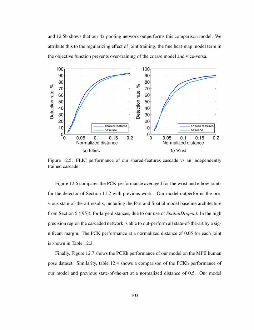
and 12.5b shows that our 4x pooling network outperforms this comparison model. We

attribute this to the regularizing effect of joint training; the fine heat-map model term in

the objective function prevents over-training of the coarse model and vice-versa.

0 0.05 0.1 0.15 0.20

10

20

30

40

50

60

70

80

90

100

Normalized distance

De

tectio

n r

ate

, %

shared features

baseline

(a) Elbow

0 0.05 0.1 0.15 0.20

10

20

30

40

50

60

70

80

90

100

Normalized distanceD

ete

ctio

n r

ate

, %

shared features

baseline

(b) Wrist

Figure 12.5: FLIC performance of our shared-features cascade vs an independentlytrained cascade

Figure 12.6 compares the PCK performance averaged for the wrist and elbow joints

for the detector of Section 11.2 with previous work . Our model outperforms the pre-

vious state-of-the-art results, including the Part and Spatial model baseline architecture

from Section 5 ([95]), for large distances, due to our use of SpatialDropout. In the high

precision region the cascaded network is able to out-perform all state-of-the-art by a sig-

nificant margin. The PCK performance at a normalized distance of 0.05 for each joint

is shown in Table 12.3.

Finally, Figure 12.7 shows the PCKh performance of our model on the MPII human

pose dataset. Similarity, table 12.4 shows a comparison of the PCKh performance of

our model and previous state-of-the-art at a normalized distance of 0.5. Our model

103

this work 4X

this work 8x

this work 16x

Tompson et al.

Toshev et al.

Jain et al.

MODEC

Yang et al.

Sapp et al.

0 0.025 0.05 0.075 0.1 0.125 0.15 0.175 0.20

10

20

30

40

50

60

70

80

90

100

Normalized distance

Dete

ction r

ate

, %

Figure 12.6: FLIC - average PCK for wrist and elbow

Head Shoulder Elbow Wrist

Yang et al. - - 22.6 15.3Sapp et al. - - 6.4 7.9Eichner et al. - - 11.1 5.2MODEC et al. - - 28.0 22.3Toshev et al. - - 25.2 26.4Jain et al. - 42.6 24.1 22.3Tompson et al. 90.7 70.4 50.2 55.4This work 4x 92.6 73.0 57.1 60.4This work 8x 92.1 75.8 55.6 56.6This work 16x 91.6 73.0 47.7 45.5

Table 12.3: Comparison with prior-art on FLIC (PCK @ 0.05)

out-performs all existing methods by a considerable margin.

104

0 0.05 0.1 0.15 0.2 0.25 0.3 0.35 0.4 0.45 0.50

10

20

30

40

50

60

70

80

90

100

Normalized distance

Dete

ction r

ate

, %

this work 4X

Pishchulin et al.

Figure 12.7: MPII - average PCKh for all joints

Head Shoulder Elbow Wrist Hip Knee Ankle Upper Body Full Body

Gkioxari et al. - 36.3 26.1 15.3 - - - 25.9 -Sapp & Taskar - 38.0 26.3 19.3 - - - 27.9 -Yang & Ramanan 73.2 56.2 41.3 32.1 36.2 33.2 34.5 43.2 44.5Pishchulin et al. 74.2 49.0 40.8 34.1 36.5 34.4 35.1 41.3 44.0This work 4x 96.0 91.9 83.9 77.7 80.9 72.2 64.8 84.5 82.0

Table 12.4: Comparison with prior-art: MPII (PCKh @ 0.5)

105

Conclusions

We have shown that discriminative ConvNet architectures are able to accurately and

efficiently estimate the pose of humans in images. While it is not clear if one architec-

ture is applicable to all problem domains, we have never-the-less shown that networks

adapted to the problem are able to out-perform existing methods via domain-specific

optimizations. We have demonstrated such optimizations on two example problem do-

mains: 1. monocular hand-pose recognition from depth images and 2. monocular full

body-pose recognition from RGB images.

In Part I we presented a novel pipeline for tracking the instantaneous pose of artic-

ulable objects from a single depth image. As an application of this pipeline we showed

state-of-the-art results for tracking human hands in real-time using commodity hard-

ware. This pipeline leverages the accuracy of offline model-based dataset generation

routines in support of a robust real-time ConvNet architecture for feature extraction.

We showed that it is possible to use intermediate heat-map features to extract accurate

and reliable 3D pose information at interactive frame-rates using inverse kinematics. To

build the ConvNet architecture we applied domain-specific applications related to the

human hand and since it is possible to use the output of the RDF stage to crop, center

and scale the incoming depth image around the hand, we showed that it is possible to use

a large fully-connected layer in the network architecture without significant overtraining

(since translation invariance need not be learned).

Building upon the results from Part I, in Parts II, III and IV we applied an adapted

sliding-window based ConvNet architecture to the problem of full-body tracking in

monocular RGB images. For this application we did not have access to a depth image

source, however we were able to incorporate connectivity priors to improve the ConvNet

106

architecture as a domain-specific optimization. This was achieved via a novel ConvNet

Part-Detector and an MRF inspired Spatial-Model which can be efficiently incorporated

into a single learning framework. This new network paradigm significantly outperforms

existing architectures on the task of human body pose recognition. Training and infer-

ence of our architecture uses commodity level hardware and runs at close to real-time

frame rates, making this technique tractable for a wide variety of application areas. For

future work we expect to further improve upon these results by increasing the complex-

ity and expressiveness of our simple spatial model (especially for unconstrained datasets

like LSP and MPII).

In Part II we showed that when incorporating both RGB and motion features in

our deep ConvNet architecture, our network is able to outperform existing state-of-the-

art techniques for the task of human body pose detection in video and improve upon

the baseline model of Part I. We have also shown that using motion features alone can

outperform some traditional algorithms [27, 105, 80]. Our findings suggest that even

very simple temporal cues can greatly improve performance with a very minor increase

in model complexity. As such, we suggest that future work should place more emphasis

on the correct use of motion features. We would also like to further explore higher

level temporal features, potentially via learned spatiotemporal convolution stages and

we hope that using a more expressive temporal-spatial model (using motion constraints)

will help improve performance significantly.

Though originally developed for the task of classification [56], Deep ConvNet have

been successfully applied to a multitude of other problems. In classification all vari-

ability except the object identity is suppressed. On the other hand, localization tasks

such as human body pose estimation often demand a high degree of spatial precision.

In Part III we presented a domain-specific optimization that is able to efficiently recover

107

the precision lost due to pooling in traditional ConvNet architectures while maintaining

the computational benefits of pooling. We presented a novel cascaded architecture that

combined fine and coarse scale convolutional networks, which achieved new state-of-

the-art results on the FLIC [79] and MPII-human-pose[5] datasets.

108

Bibliography

[1] 3Gear. 3Gear Sytems Hand-Tracking Development Platform. 2014.

[2] A. Agarwal, B. Triggs, I. Rhone-Alpes, and F. Montbonnot. “Recovering 3Dhuman pose from monocular images”. In: PAMI. 2006.

[3] Brett Allen, Brian Curless, and Zoran Popovic. “The space of human bodyshapes: reconstruction and parameterization from range scans”. In: ACM TOG.2003.

[4] M. Andriluka, S. Roth, and B. Schiele. “Pictorial structures revisited: Peopledetection and articulated pose estimation”. In: CVPR. 2009.

[5] Mykhaylo Andriluka, Leonid Pishchulin, Peter Gehler, and Bernt Schiele. “2DHuman Pose Estimation: New Benchmark and State of the Art Analysis”. In:CVPR. 2014.

[6] Dragomir Anguelov, Praveen Srinivasan, Daphne Koller, Sebastian Thrun, JimRodgers, and James Davis. “Scape: shape completion and animation of people”.In: ACM TOG. 2005.

[7] Luca Ballan, Aparna Taneja, Jurgen Gall, Luc Van Gool, and Marc Pollefeys.“Motion capture of hands in action using discriminative salient points”. In:ECCV. 2012.

109

[8] M. Bergtholdt, J. Kappes, S. Schmidt, and C. Schnorr. “A study of parts-basedobject class detection using complete graphs”. In: IJCV. 2010.

[9] L. Bourdev and J. Malik. “Poselets: Body Part Detectors Trained Using 3D Hu-man Pose Annotations”. In: ICCV. 2009.

[10] H. Bourlard, Y. Konig, and N. Morgan. “REMAP: recursive estimation and max-imization of a posteriori probabilities in connectionist speech recognition.” In:EUROSPEECH. 1995.

[11] Yuri Boykov, Olga Veksler, and Ramin Zabih. “Fast Approximate Energy Min-imization via Graph Cuts”. In: PAMI. 2001.

[12] Christoph Bregler and Jitendra Malik. “Tracking people with twists and expo-nential maps”. In: CVPR. 1998.

[13] Jane Bromley, James W Bentz, Leon Bottou, Isabelle Guyon, Yann LeCun, CliffMoore, Eduard Sackinger, and Roopak Shah. “Signature verification using aSiamese? time delay neural network”. In: PRAI. 1993.

[14] P. Buehler, A. Zisserman, and M. Everingham. “Learning sign language bywatching TV (using weakly aligned subtitles)”. In: CVPR. 2009.

[15] D. Alex Butler, Shahram Izadi, Otmar Hilliges, David Molyneaux, SteveHodges, and David Kim. “Shake’n’sense: reducing interference for overlappingstructured light depth cameras”. In: ACM HFCS. 2012.

[16] Xianjie Chen and Alan Yuille. “Articulated Pose Estimation by a GraphicalModel with Image Dependent Pairwise Relations”. In: NIPS. 2014.

[17] K. Cho, B. van Merrienboer, C. Gulcehre, D. Bahdanau, F. Bougares, H.Schwenk, and Y. Bengio. “Learning Phrase Representations using RNN EncoderDecoder for Statistical Machine Translation”. In: EMNLP. 2014.

110

[18] R. Collobert, K. Kavukcuoglu, and C. Farabet. “Torch7: A Matlab-like Environ-ment for Machine Learning”. In: NIPS Workshop. 2011.

[19] Camille Couprie, Clement Farabet, Laurent Najman, and Yann LeCun. “IndoorSemantic Segmentation using depth information”. In: ICLR. 2013.

[20] N. Dalal and B. Triggs. “Histograms of Oriented Gradients for Human Detec-tion”. In: CVPR. 2005.

[21] N. Dalal, B. Triggs, and C. Schmid. “Human detection using oriented histogramsof flow and appearance”. In: ECCV. 2006.

[22] M. Dantone, J. Gall, C. Leistner, and L. Van Gool. “Human Pose Estimationusing Body Parts Dependent Joint Regressors”. In: CVPR. 2013.

[23] Christian Puhrsch David Eigen and Rob Fergus. “Depth Map Prediction from aSingle Image using a Multi-Scale Deep Network”. In: NIPS. 2014.

[24] Edilson De Aguiar, Carsten Stoll, Christian Theobalt, Naveed Ahmed, Hans-Peter Seidel, and Sebastian Thrun. “Performance capture from sparse multi-view video”. In: TOG. 2008.

[25] Jia Deng, Wei Dong, Richard Socher, Li-Jia Li, Kai Li, and Li Fei-Fei. “Ima-genet: A large-scale hierarchical image database”. In: CVPR. 2009.

[26] Jonathan Deutscher, Andrew Blake, and Ian Reid. “Articulated body motioncapture by annealed particle filtering”. In: CVPR. 2000.

[27] M. Eichner and V. Ferrari. “Better Appearance Models For Pictorial Structures”.In: BMVC. 2009.

[28] Ali Erol, George Bebis, Mircea Nicolescu, Richard D Boyle, and XanderTwombly. “Vision-based hand pose estimation: A review”. In: CVIU. 2007.

111

[29] C. Farabet, C. Couprie, L. Najman, and Y. LeCun. “Learning Hierarchical Fea-tures for Scene Labeling”. In: PAMI. 2013.

[30] P. Felzenszwalb, D. McAllester, and D. Ramanan. “A discriminatively trained,multiscale, deformable part model”. In: CVPR. 2008.

[31] V. Ferrari, M. Marin-Jimenez, and A. Zisserman. “Progressive Search SpaceReduction for Human Pose Estimation”. In: CVPR. 2008.

[32] Martin A. Fischler and R.A. Elschlager. “The Representation and Matching ofPictorial Structures”. In: IEEE TOC. 1973.

[33] William T Freeman and Michal Roth. “Orientation histograms for hand gesturerecognition”. In: FG. 1995.

[34] A. Giusti, D. Ciresan, J. Masci, L. Gambardella, and J. Schmidhuber. “FastImage Scanning with Deep Max-Pooling Convolutional Neural Networks”. In:CoRR. 2013.

[35] G. Gkioxari, P. Arbelaez, L. Bourdev, and J. Malik. “Articulated Pose Estimationusing Discriminative Armlet Classifiers”. In: CVPR. 2013.

[36] K. Grauman, G. Shakhnarovich, and T. Darrell. “Inferring 3D Structure with aStatistical Image-Based Shape Model”. In: ICCV. 2003.

[37] Caglar Gulcehre. Deep Learning Reading List. deeplearning.net/reading-list/.2015.

[38] G. Heitz, S. Gould, A. Saxena, and D. Koller. “Cascaded Classification Models:Combining Models for Holistic Scene Understanding”. In: NIPS. 2008.

[39] Geoffrey E Hinton, Nitish Srivastava, Alex Krizhevsky, Ilya Sutskever, and Rus-lan R Salakhutdinov. “Improving neural networks by preventing co-adaptationof feature detectors”. In: arXiv preprint arXiv:1207.0580. 2012.

112

[40] David Hogg. “Model-based vision: a program to see a walking person”. In: ICV.1983.

[41] Berthold K. P. Horn. “Closed-form solution of absolute orientation using unitquaternions”. In: JOSA. 1987.

[42] Arjun Jain, Thorsten Thormahlen, Hans-Peter Seidel, and Christian Theobalt.“Moviereshape: Tracking and reshaping of humans in videos”. In: TOG. 2010.

[43] Arjun Jain, Jonathan Tompson, Micha Andriluka, Graham Taylor, and ChristophBregler. “Learning Human Pose Estimation Features with Convolutional Net-works”. In: ICLR. 2014.

[44] Arjun Jain, Jonathan Tompson, Yann LeCun, and Christoph Bregler. “MoDeep:A Deep Learning Framework Using Motion Features for Human Pose Estima-tion”. In: ACCV. 2014.

[45] K. Jarrett, K. Kavukcuoglu, M. Ranzato, and Y. LeCun. “What is the best multi-stage architecture for object recognition?” In: ICCV. 2009.

[46] Mingyuan Jiu, Christian Wolf, Graham W. W. Taylor, and Atilla Baskurt. “Hu-man body part estimation from depth images via spatially-constrained deeplearning”. In: Pattern Recognition Letters. 2013.

[47] G. Johansson. “Visual perception of biological motion and a model for its anal-ysis”. In: Perception and Psychophysics. 1973.

[48] S. Johnson and M. Everingham. “Clustered Pose and Nonlinear AppearanceModels for Human Pose Estimation”. In: BMVC. 2010.

[49] S. Johnson and M. Everingham. “Learning Effective Human Pose Estimationfrom Inaccurate Annotation”. In: CVPR. 2011.

113

[50] Ioannis A Kakadiaris and Dimitris Metaxas. “Model-based estimation of 3Dhuman motion with occlusion based on active multi-viewpoint selection”. In:CVPR. 1996.

[51] Andrej Karpathy, George Toderici, Sanketh Shetty, Thomas Leung, Rahul Suk-thankar, and Li Fei-Fei. “Large-scale Video Classification with ConvolutionalNeural Networks”. In: CVPR. 2014.

[52] C. Keskin, F. Kirac, Y.E. Kara, and L. Akarun. “Real time hand pose estimationusing depth sensors”. In: ICCV workshop. 2011.

[53] Cem Keskin, Furkan Kirac, Yunus Emre Kara, and Lale Akarun. “Hand Pose Es-timation and Hand Shape Classification Using Multi-layered Randomized Deci-sion Forests”. In: ECCV. 2012.

[54] Alex Krizhevsky, Ilya Sutskever, and Geoff Hinton. “ImageNet Classificationwith Deep Convolutional Neural Networks”. In: NIPS. 2012.

[55] Ivan Laptev. “On Space-Time Interest Points”. In: IJCV. 2005.

[56] Y. LeCun, L. Bottou, Y. Bengio, and P. Haffner. “Gradient-based learning ap-plied to document recognition”. In: Proceedings of the IEEE. 1998.

[57] Y. LeCun, Fu Jie Huang, and L. Bottou. “Learning methods for generic objectrecognition with invariance to pose and lighting”. In: CVPR. 2004.

[58] Hao Li, Robert W. Sumner, and Mark Pauly. “Global Correspondence Optimiza-tion for Non-Rigid Registration of Depth Scans”. In: SGP. 2008.

[59] Hao Li, Jihun Yu, Yuting Ye, and Chris Bregler. “Realtime Facial Animationwith On-the-fly Correctives”. In: ACM TOG. 2013.

[60] D. Lowe. “Object recognition from local scale-invariant features”. In: ICCV.1999.

114

[61] David G. Lowe. “Distinctive Image Features from Scale-Invariant Keypoints”.In: IJCV. 2004.

[62] M. Mathieu, M. Henaff, and Y. LeCun. “Fast Training of Convolutional Net-works through FFTs”. In: CoRR. 2013.

[63] Y. Matsushita, E. Ofek, Weina Ge, Xiaoou Tang, and Heung-Yeung Shum. “Full-frame video stabilization with motion inpainting”. In: PAMI. 2006.

[64] Stan Melax, Leonid Keselman, and Sterling Orsten. “Dynamics based 3D skele-tal hand tracking”. In: i3D. 2013.

[65] G. Mori and J. Malik. “Estimating human body configurations using shape con-text matching”. In: ECCV. 2002.

[66] F. Morin and Y. Bengio. “Hierarchical Probabilistic Neural Network LanguageModel”. In: AISTATS workshop. 2005.

[67] J. Nagi, F. Ducatelle, G.A. Di Caro, D. Ciresan, U. Meier, A. Giusti, F. Nagi, J.Schmidhuber, and L.M. Gambardella. “Max-pooling convolutional neural net-works for vision-based hand gesture recognition”. In: ICSIPA. 2011.

[68] F. Ning, D. Delhomme, Y. LeCun, F. Piano, L. Bottou, and P. Barbano. “TowardAutomatic Phenotyping of Developing Embryos from Videos”. In: IEEE TIP.2005.

[69] Steven J. Nowlan and John C. Platt. “A Convolutional Neural Network HandTracker”. In: NIPS. 1995.

[70] I. Oikonomidis, N. Kyriazis, and A. Argyros. “Efficient model-based 3D track-ing of hand articulations using Kinect”. In: BMVC. 2011.

115

[71] Margarita Osadchy, Yann LeCun, Matthew L. Miller, and Pietro Perona. “Syn-ergistic face detection and pose estimation with energy-based model”. In: NIPS.2005.

[72] L. Pishchulin, M. Andriluka, P. Gehler, and B. Schiele. “Poselet ConditionedPictorial Structures”. In: CVPR. 2013.

[73] L. Pishchulin, M. Andriluka, P. Gehler, and B. Schiele. “Strong Appearance andExpressive Spatial Models for Human Pose Estimation”. In: ICCV. 2013.

[74] R. Poppe. “Vision-based human motion analysis: An overview”. In: CVIU.2007.

[75] D. Ramanan, D. Forsyth, and A. Zisserman. “Strike a pose: Tracking people byfinding stylized poses”. In: CVPR. 2005.

[76] James M Rehg and Takeo Kanade. “Model-based tracking of self-occluding ar-ticulated objects”. In: ICCV. 1995.

[77] James M. Rehg and Takeo Kanade. “Visual Tracking of High DOF ArticulatedStructures: an Application to Human Hand Tracking”. In: ECCV. 1994.

[78] S. Ross, D. Munoz, M. Hebert, and J.A Bagnell. “Learning message-passinginference machines for structured prediction”. In: CVPR. 2011.

[79] Ben Sapp and Ben Taskar. “MODEC: Multimodal decomposable models forhuman pose estimation”. In: CVPR. 2013.

[80] Benjamin Sapp, Alexander Toshev, and Ben Taskar. “Cascaded Models for Ar-ticulated Pose Estimation”. In: ECCV. 2010.

[81] Marin Saric. LibHand: A Library for Hand Articulation. version 0.9. 2011. url:http://www.libhand.org/.

116

http://www.libhand.org/

[82] P. Sermanet, D. Eigen, X. Zhang, M. Mathieu, R. Fergus, and Y. LeCun. “Over-Feat: Integrated Recognition, Localization and Detection using ConvolutionalNetworks”. In: ICLR. 2014.

[83] Pierre Sermanet, Koray Kavukcuoglu, Soumith Chintala, and Yann LeCun.“Pedestrian Detection with Unsupervised Multi-stage Feature Learning”. In:CVPR. 2013.

[84] Gregory Shakhnarovich, Paul Viola, and Trevor Darrell. “Fast pose estimationwith parameter sensitive hashing”. In: ICCV. 2003.

[85] Jamie Shotton, Toby Sharp, Alex Kipman, Andrew Fitzgibbon, Mark Finocchio,Andrew Blake, Mat Cook, and Richard Moore. “Real-time human pose recog-nition in parts from single depth images”. In: CVPR. 2013.

[86] Hedvig Sidenbladh, Michael J Black, and David J Fleet. “Stochastic tracking of3D human figures using 2D image motion”. In: ECCV. 2000.

[87] L. Sigal, A. Balan, and Black. M. J. “HumanEva: Synchronized video and mo-tion capture dataset and baseline algorithm for evaluation of articulated humanmotion”. In: IJCV. 2010.

[88] Cristian Sminchisescu and Bill Triggs. “Covariance scaled sampling for monoc-ular 3D body tracking”. In: CVPR. 2001.

[89] Murphy Stein, Jonathan Tompson, Xiao Xiao, Charley Hendeee, Hiroshi Ishii,and Ken Perlin. “ARCADE: a system for augmenting gesture-based computergraphic presentations”. In: SIGGRAPH Computer Animation Festival. 2012.

[90] Carsten Stoll, Nils Hasler, Juergen Gall, H Seidel, and Christian Theobalt. “Fastarticulated motion tracking using a sums of gaussians body model”. In: ICCV.2011.

[91] Ilya Sutskever, Oriol Vinyals, and Quoc V. Le. “Sequence to Sequence Learningwith Neural Networks”. In: NIPS. 2014.

117

[92] C. Szegedy, W. Liu, Y. Jia, P. Sermanet, S. Reed, D. Anguelov, D. Erhan, V.Vanhoucke, and A. Rabinovich. “Going Deeper with Convolutions”. In: CVPR.2014.

[93] Graham W. Taylor, Ian Spiro, Christoph Bregler, and Rob Fergus. “Learninginvariance through imitation”. In: CVPR. 2011.

[94] Jonathan Tompson, Ross Goroshin, Arjun Jain, Yann LeCun, and Christoph Bre-gler. “Efficient Object Localization Using Convolutional Networks”. In: arxiv.2015.

[95] Jonathan Tompson, Arjun Jain, Yann LeCun, and Christoph Bregler. “Join Train-ing of a Convolutional Network and a Graphical Model for Human Pose Esti-mation”. In: NIPS. 2014.

[96] Jonathan Tompson, Murphy Stein, Yann LeCun, and Ken Perlin. “Real-TimeContinuous Pose Recovery of Human Hands Using Convolutional Networks”.In: TOG. 2014.

[97] A. Toshev and C. Szegedy. “DeepPose: Human Pose Estimation via Deep Neu-ral Networks”. In: CVPR. 2014.

[98] Paul Tseng. Fortified-Descent Simplicial Search Method: A General Approach.Tech. rep. SIAM booktitle of Optimization, 1995.

[99] Robert Y. Wang and Jovan Popovic. “Real-time hand-tracking with a colorglove”. In: SIGGRAPH. 2009.

[100] Robert Wang, Sylvain Paris, and Jovan Popovic. “6D hands: markerless hand-tracking for computer aided design”. In: UIST. 2011.

[101] Philippe Weinzaepfel, Jerome Revaud, Zaid Harchaoui, and Cordelia Schmid.“DeepFlow: Large displacement optical flow with deep matching”. In: ICCV.2013.

118

[102] Thibaut Weise, Hao Li, Luc Van Gool, and Mark Pauly. “Face/Off: Live FacialPuppetry”. In: Eurographics. 2009.

[103] David Weiss, Benjamin Sapp, and Ben Taskar. “Sidestepping Intractable Infer-ence with Structured Ensemble Cascades”. In: NIPS. 2010.

[104] C. Wren, A. Azarbayejani, T. Darrell, and A. Pentland. “Pfinder: Real-timetracking of the human body”. In: PAMI. 1997.

[105] Yi Yang and Deva Ramanan. “Articulated pose estimation with flexible mixturesof parts”. In: CVPR. 2011.

[106] T. Yasuda, K. Ohkura, and Y. Matsumura. “Extended PSO with partial random-ization for large scale multimodal problems”. In: WAC. 2010.

[107] Wenping Zhao, Jinxiang Chai, and Ying-Qing Xu. “Combining Marker-basedMocap and RGB-D Camera for Acquiring High-fidelity Hand Motion Data”.In: Eurographics. 2012.

119

Localization of Humans in Images Using Convolutional ...

Documents

Transcript of Localization of Humans in Images Using Convolutional ...