MD-Recon-Net: A Parallel Dual-Domain Convolutional Neural ...
17
1 Abstract—Compressed sensing magnetic resonance imaging (CS-MRI) is a theoretical framework that can accurately reconstruct images from undersampled k-space data with a much lower sampling rate than the one set by the classical Nyquist-Shannon sampling theorem. Therefore, CS-MRI can efficiently accelerate acquisition time and relieve the psychological burden on patients while maintaining high imaging quality. The problems with traditional CS-MRI reconstruction are solved by iterative numerical solvers, which usually suffer from expensive computational cost and the lack of accurate handcrafted priori. In this paper, inspired by deep learning’s (DL’s) fast inference and excellent end-to-end performance, we propose a novel cascaded convolutional neural network called MD-Recon-Net to facilitate fast and accurate MRI reconstruction. Especially, different from existing DL- based methods, which operate on single domain data or both domains in a certain order, our proposed MD-Recon- Net contains two parallel and interactive branches that simultaneously perform on k-space and spatial-domain data, exploring the latent relationship between k-space and the spatial domain. The simulated experimental results show that the proposed method not only achieves competitive visual effects to several state-of-the-art methods, but also outperforms other DL-based methods in terms of model scale and computational cost. Index Terms—Magnetic resonance imaging (MRI), compressed sensing, MRI reconstruction, information fusion, convolutional neural network I. INTRODUCTION agnetic resonance imaging (MRI) is a mainstream medical imaging technology that can reveal both internal anatomical structures and physiological functions noninvasively. Although MRI is superior to other medical imaging modalities in terms of both soft-tissue contrast and resolution, MRI’s sampling process in k-space suffers from prolonged acquisition time due to physiological and hardware constraints. Even worse, such long sampling time causes patients discomfort and potentially leads to motion artifacts. These limitations make MRI unsuitable for time-critical diagnostics such as stroke. Meanwhile, hybrid PET/MR imaging is growing in several clinical applications, such as early diagnosis for tumors and cardio-cerebral diseases [1-3]. Since the PET scan is much faster than MR, the imaging speed of PET/MR is dominated by the MR scan. As a result, efficient reconstruction algorithms that accelerate MRI are in high demand. Over the past few years, various efforts have been made to develop advanced reconstruction algorithms to reduce the acquisition time in MRI. These methods fall into two categories: the first one is hardware-based parallel MRI (pMRI) [4], which uses phased array coils containing multiple independent receiver channels [5]. Each coil has sensitivity to measure raw data from an individual tissue type, which requires specific MD-Recon-Net: A Parallel Dual-Domain Convolutional Neural Network for Compressed Sensing MRI Maosong Ran, Wenjun Xia, Yongqiang Huang, Zexin Lu, Peng Bao, Yan Liu, Huaiqiang Sun, Jiliu Zhou, Senior Member, IEEE, and Yi Zhang * , Senior Member, IEEE This work was supported in part by the National Natural Science Foundation of China under Grant 61671312, in part by the Sichuan Science and Technology Program under Grant 2018HH0070. (Corresponding author: Yi Zhang) M. Ran, W. Xia, Y. Huang, Z. Lu, P. Bao, J. Zhou and Y. Zhang are with th e College of Computer Science, Sichuan University, Chengdu 610065, China (e-mail: [email protected]; [email protected]; hyq_tsmotlp@163. com; [email protected]; [email protected]; [email protected]; [email protected] ) Y. Liu is with the School of Electrical Engineering Information, Sichuan Un iversity, Chengdu 610065, China(e-mail: [email protected]) H. Sun is with the Department of Radiology, West China Hospital of Sichua n University, Chengdu 610041, China (e-mail: [email protected]) M NN NN NN IFT (a) (b) (d) (e) NN IFT IFT NN Fig.1 DL-based methods for fast MRI. (a) Spatial-domain based methods; (b) k-space based methods; (c) iteration unrolling methods; (d) directly mapping from k-space to image; (e) cross-domain reconstruction. NN: Neural Network, IFT: Inverse Fourier Transform. NN IFT FT ⊕ (c)
-
Upload
khangminh22 -
Category
Documents
-
view
2 -
download
0
Transcript of MD-Recon-Net: A Parallel Dual-Domain Convolutional Neural ...
1
Abstract—Compressed sensing magnetic resonance
imaging (CS-MRI) is a theoretical framework that can
accurately reconstruct images from undersampled k-space
data with a much lower sampling rate than the one set by
the classical Nyquist-Shannon sampling theorem. Therefore,
CS-MRI can efficiently accelerate acquisition time and
relieve the psychological burden on patients while
maintaining high imaging quality. The problems with
traditional CS-MRI reconstruction are solved by iterative
numerical solvers, which usually suffer from expensive
computational cost and the lack of accurate handcrafted
priori. In this paper, inspired by deep learning’s (DL’s) fast
inference and excellent end-to-end performance, we
propose a novel cascaded convolutional neural network
called MD-Recon-Net to facilitate fast and accurate MRI
reconstruction. Especially, different from existing DL-
based methods, which operate on single domain data or
both domains in a certain order, our proposed MD-Recon-
Net contains two parallel and interactive branches that
simultaneously perform on k-space and spatial-domain data,
exploring the latent relationship between k-space and the
spatial domain. The simulated experimental results show
that the proposed method not only achieves competitive
visual effects to several state-of-the-art methods, but also
outperforms other DL-based methods in terms of model
scale and computational cost.
Index Terms—Magnetic resonance imaging (MRI), compressed
sensing, MRI reconstruction, information fusion, convolutional
neural network
I. INTRODUCTION
agnetic resonance imaging (MRI) is a mainstream
medical imaging technology that can reveal both internal
anatomical structures and physiological functions
noninvasively. Although MRI is superior to other medical
imaging modalities in terms of both soft-tissue contrast and
resolution, MRI’s sampling process in k-space suffers from
prolonged acquisition time due to physiological and hardware
constraints. Even worse, such long sampling time causes
patients discomfort and potentially leads to motion artifacts.
These limitations make MRI unsuitable for time-critical
diagnostics such as stroke. Meanwhile, hybrid PET/MR
imaging is growing in several clinical applications, such as
early diagnosis for tumors and cardio-cerebral diseases [1-3].
Since the PET scan is much faster than MR, the imaging speed
of PET/MR is dominated by the MR scan. As a result, efficient
reconstruction algorithms that accelerate MRI are in high
demand.
Over the past few years, various efforts have been made to
develop advanced reconstruction algorithms to reduce the
acquisition time in MRI. These methods fall into two categories:
the first one is hardware-based parallel MRI (pMRI) [4], which
uses phased array coils containing multiple independent
receiver channels [5]. Each coil has sensitivity to measure raw
data from an individual tissue type, which requires specific
MD-Recon-Net: A Parallel Dual-Domain Convolutional
Neural Network for Compressed Sensing MRI
Maosong Ran, Wenjun Xia, Yongqiang Huang, Zexin Lu, Peng Bao, Yan Liu, Huaiqiang Sun, Jiliu Zhou, Senior
Member, IEEE, and Yi Zhang*, Senior Member, IEEE
This work was supported in part by the National Natural Science Foundation
of China under Grant 61671312, in part by the Sichuan Science and Technology
Program under Grant 2018HH0070. (Corresponding author: Yi Zhang)
M. Ran, W. Xia, Y. Huang, Z. Lu, P. Bao, J. Zhou and Y. Zhang are with th
e College of Computer Science, Sichuan University, Chengdu 610065, China
(e-mail: [email protected]; [email protected]; hyq_tsmotlp@163.
com; [email protected]; [email protected]; [email protected];
Y. Liu is with the School of Electrical Engineering Information, Sichuan Un
iversity, Chengdu 610065, China(e-mail: [email protected])
H. Sun is with the Department of Radiology, West China Hospital of Sichua
n University, Chengdu 610041, China (e-mail: [email protected])
M
NN
NN
NN
IFT
(a)
(b)
(d)
(e)
NN IFT
IFT
NN
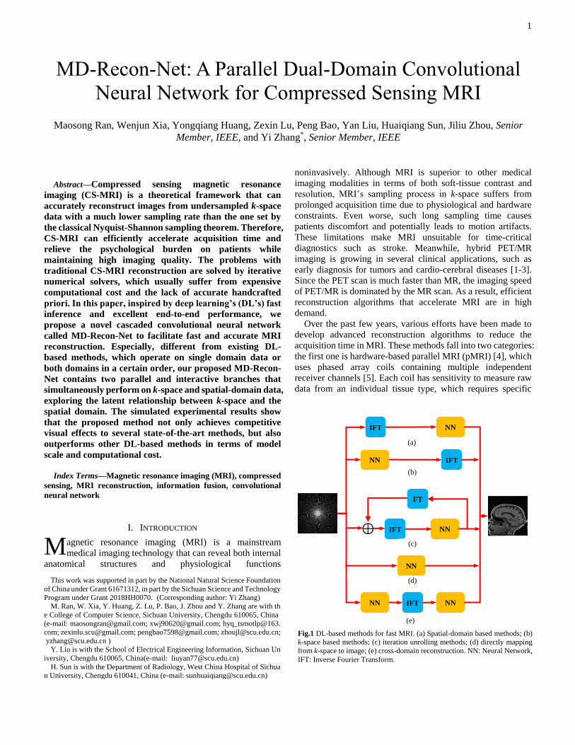
Fig.1 DL-based methods for fast MRI. (a) Spatial-domain based methods; (b)
k-space based methods; (c) iteration unrolling methods; (d) directly mapping
from k-space to image; (e) cross-domain reconstruction. NN: Neural Network,
IFT: Inverse Fourier Transform.
NN IFT
FT
⊕ (c)
2
pMRI reconstruction algorithms. These pMRI reconstruction
methods can be classified into three groups: (a) image domain
based methods, such as SENSE [6, 7] and its variants [8-11]; (b)
k-space based methods, such as SMASH [12-14] and GRAPPA
[15]; and (c) combinations of the previous two kinds of methods,
such as SPACE-RIP [16] and SPIRiT [17]. Despite wide
clinical application, pMRI still has modest acceleration rates.
The second acceleration strategy is based on the theory of
compressed sensing (CS) [18], called compressed sensing
magnetic resonance imaging (CS-MRI) [8, 19]. Because the
acceleration rate is proportional to the sampling ratio, CS-MRI
tries to accelerate reconstruction with undersampled k-space
data at a rate much lower than the one set by the classical
Nyquist-Shannon sampling theorem. In the sense of CS-MRI,
the image to reconstruct is assumed to be sparse after
application of a certain sparsifying transform. Typical
transforms include Fourier transform (FT), wavelet, total
variation (TV), and low-rank[8, 18-20]. Recently, two data-
driven based CS methods, dictionary learning and transform
learning, have been introduced to improve the performance of
CS-MRI [21-23]. Although these methods have achieved
considerable success, several critical drawbacks still hamper
the clinical practice of CS-MRI: (i) the iterative procedure is
time consuming. A complex regularization term would even
further aggravate the cost; (ii) parametric adjustment is
exhausting for users; and (iii) the handcrafted regularization
terms cannot ensure consistently superior performance for all
scanning protocols and patients because of the lack of accurate
prior information.
In recent years, the success of deep learning (DL) has
suggested a new orientation in fast MRI reconstruction. DL-
based fast MRI has gained much attention, and many new
methods have emerged. These methods can be roughly divided
into five groups according to data processing and specific
pipeline. The basic flowcharts are illustrated in Fig. 1. The first
group as shown in Fig. 1(a) is post-processing algorithms that
use the inverse Fourier transform (IFT) to obtain an initial
image as the first input to the network. In this group, the
network model acts a role of an image-to-image mapping
function [24-28]. For examples, [25, 28] are the earliest works
to introduce generative adversarial network (GAN) into post-
processing based fast MRI reconstruction. [28] added a data
consistency layer to ensure the points on the realistic data
manifold. [24] used a deeper generator and discriminator
networks with cyclic data consistency loss to further enhance
the imaging quality. This kind of method is the mainstream of
current DL-based models, as it is convenient to insert into the
current workflow of commercial scanners. In contrast, the
second class as shown in Fig. 1(b) directly deals with the
undersampled k-space data using a neural network, and after
that, IFT is applied to obtain the final results [29]. Because any
artifacts introduced by the network may spread to the whole
reconstructed image, this kind of method has not been widely
studied yet. The third branch in Fig. 1(c) comprises the iteration
unrolling methods [30-34]. Specifically, in [34], the data
consistency lay was embedded into the unrolling iteration
network and the same group improved the former network by
introducing dilated convolution and stochastic architecture [33].
In these methods, different iterative numerical solvers are
treated as different recurrent networks, and the learned
regularization terms constrain the image in terms of each
intermediate reconstructed result. Fig. 1(d) includes methods
that directly learn the image from the undersampled k-space
data [35]. Fully connected layers are usually needed for this
kind of model, and the network scale is generally huge. Until
now, all the methods mentioned above have all performed in a
single domain and have not fully explored the latent
relationship between k-space and the spatial domain. The last
pipeline illustrated in Fig. 1(e) has gained much attention very
recently. This type of method attempts to explore the
information in both k-space and the spatial domain [36-38]. It
usually adopts two cascaded networks performing on k-space
and spatial-domain data, with IFT employed to build the bridge
between the two networks. Currently, state-of-the-art
performance is achieved using such dual-domain based
methods. However, existing dual-domain methods [36-38]
process the k-space and spatial-domain data sequentially, which
implicitly adds a certain priority priori into the reconstruction
and may ignore the internal interplay between both domains. In
this paper, to essentially address the intrinsic relation between
the k-space and spatial domains, we propose a novel MRI Dual-
domain Reconstruction Network (MD-Recon-Net) to
accelerate magnetic resonance imaging. Different from current
methods, the proposed MD-Recon-Net contains two parallel
and interactive branches that simultaneously operate on k-space
and spatial-domain data. Data consistency layers are included
to improve performance further. At the end, dual-domain fusion
layers combine the results from the two branches.
The rest of this paper is organized as follows. Related works
and the proposed network are described in Section 2. The
experiments and evaluation are presented in Section 3. The final
section concludes this paper.
II. METHODS
A. Notations
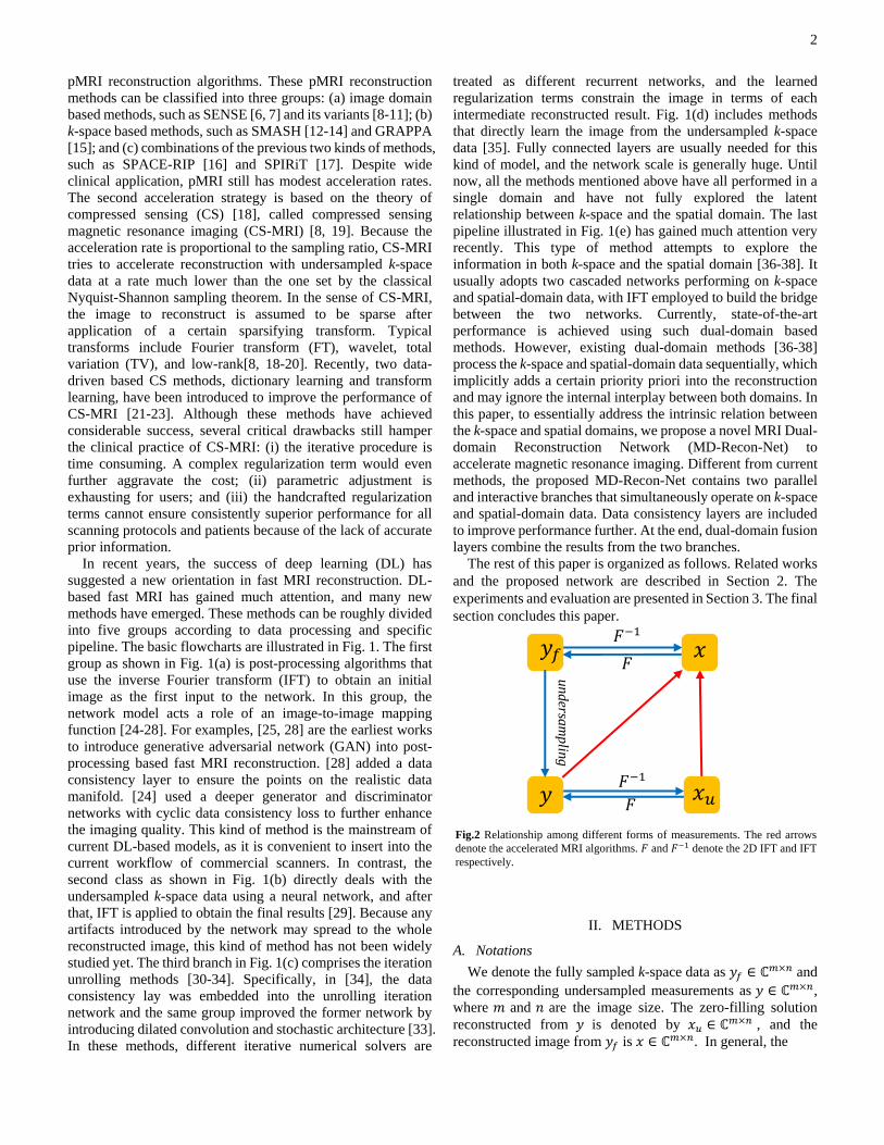
We denote the fully sampled k-space data as 𝑦𝑓 ∈ ℂ𝑚×𝑛 and
the corresponding undersampled measurements as 𝑦 ∈ ℂ𝑚×𝑛,
where 𝑚 and 𝑛 are the image size. The zero-filling solution
reconstructed from 𝑦 is denoted by 𝑥𝑢 ∈ ℂ𝑚×𝑛 , and the
reconstructed image from 𝑦𝑓 is 𝑥 ∈ ℂ𝑚×𝑛. In general, the
𝑦𝑓
𝑦
𝑥
𝑥𝑢
𝐹−1
𝐹
𝐹−1
𝐹
Fig.2 Relationship among different forms of measurements. The red arrows
denote the accelerated MRI algorithms. 𝐹 and 𝐹−1 denote the 2D IFT and IFT
respectively.
un
dersa
mp
ling
3
problem of image reconstruction can be approximately treated
as solving a linear system formulated as:
𝑦 = 𝑈 ⊙ 𝑦𝑓 + 𝜖 = 𝑈 ⊙ 𝐹𝑥 + 𝜖 = 𝐹𝑢𝑥 + 𝜖 (1)
where 𝐹 denotes the 2D FT operator, 𝑈 ∈ 𝑅𝑚×𝑛 represents the
binary undersampling mask, 𝐹𝑢 = 𝑈 ⊙ 𝐹 denotes the
undersampling Fourier encoding operator, ⊙ is element-wise
multiplication, and ϵ is acquisition noise. Fig. 2 illustrates the
relationships among different data forms, and the red arrows
indicate the accelerated MRI algorithms on which we focus
here.
B. CS-MRI
To solve the ill-posed problem in (1), classic model-based
CS-MRI [18, 19] constrains the solution space by exploiting
some prior knowledge, and the associated optimization problem
can be expressed as the following variational minimization:
min
𝑥
1
2‖𝐹𝑢𝑥 − 𝑦‖2
2 + 𝜆ℜ(𝑥) (2)
where the first term represents data fidelity, which guarantees
consistency between the reconstruction result and the original
undersampled k-space data, ℜ(𝑥) denotes the regularization
term that constrains the least squares data fidelity term, and λ ≥0 is a balancing parameter that controls the tradeoff between the
two terms. Especially, ℜ(𝑥) is usually an 𝑙0 norm or 𝑙1 norm in
a certain sparsifying transform field, and some typical
regularizers include FT, wavelet, total variation (TV), and low-
rank[8, 18-20].
DL-based CS-MRI combines the deep learning with CS-MRI
[24-27, 29, 34, 38-40], which makes the reconstructed image
and the corresponding fully sampled image as close as possible
by optimizing the parameter set 𝜃 of the neural network. This
method can be represented as:
𝑚𝑖𝑛
𝑥𝜆‖𝑓𝑛𝑛(𝑧|𝜃) − 𝑥‖2 +
1
2‖𝐹𝑢𝑥 − 𝑦‖2
2 (3)
where 𝑓𝑛𝑛 is the network model with parameter set 𝜃, 𝑧 is the
input of the model, either 𝑦 or 𝑥𝑢, and 𝑓𝑛𝑛(𝑧|𝜃) is the output of
𝑦
Sp
ati
al
do
ma
in p
roce
ssin
g
pip
elin
e
Freq
uen
cy do
ma
in p
rocessin
g
pip
eline
CNN KF
CNN SF
IFT
FT
CNN KDC
CNN SDC
SF
IFT
reconstructed
image:𝑥
Inpu
t
Ou
tpu
t
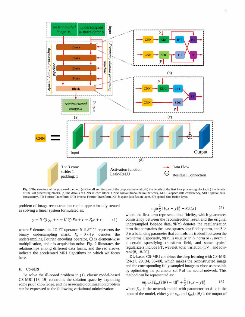
Fig. 3 The structure of the proposed method. (a) Overall architecture of the proposed network, (b) the details of the first four processing blocks, (c) the details
of the last processing blocks, (d) the details of CNN in each block. CNN: convolutional neural network, KDC: k-space data consistency, SDC: spatial data
consistency, FT: Fourier Transform, IFT: Inverse Fourier Transform, KF: k-space data fusion layer, SF: spatial data fusion layer.
𝑦
𝑦
𝑦
(b)
(c)
(d)
⨁
undersampled k-space data: 𝑦
undersampled
image:𝑥𝑢
Block
Block
Block
Block
(a)
KDC
SDC
Input Output
CNN = 3 × 3 conv
stride: 1
padding: 1
Activation function
LeakyReLU
Data Flow
Residual Connection ⨁
+
Block
4
the model, which denotes the predicted reconstruction result.
The critical part is how to design the architecture of network in
(3) as in [40] or even replace the energy minimization process
with the training process of a neural network, as in [24, 25, 36].
In this paper, we focus on the second strategy.
C. Proposed Method
In this section, we elaborate on the details of the proposed
MD-Recon-Net and introduce the network’s key components.
1) Network Architecture
The detailed architecture of the proposed MD-Recon-Net is
illustrated in Fig. 3(a). It consists of five basic blocks, and all
blocks share the same structure except for the last block. The
network takes both undersampled k-space data 𝑦 and zero-
filling reconstruction 𝑥𝑢 as input and predicts the full-sampling
reconstruction 𝑥. The proposed network contains two branches
to process the k-space and spatial data separately.
The overall structures of the basic processing blocks are
illustrated in Fig. 3(b) and (c). The block structure is key to the
proposed method and is the main contribution of this paper. The
first four blocks share the same structure, which is shown in Fig.
3(b). This block contains the following components: CNN, FT,
IFT, k-space data consistency (KDC), spatial data consistency
(SDC), k-space fusion (KF), and spatial fusion (SF) layers.
Each block accepts two inputs, k-space and spatial data, and
contains two CNN modules, which are used to extract and
recover the features in both domains. The details of the CNN
are shown in Fig. 3(d). It consists of 5 convolutional layers with
32, 32, 32, 32, and 2 filters, respectively. Residual connection
[41] is introduced to accelerate the training procedure and
preserve more detail. Because MR data are complex valued,
two channels are used to represent the real and imaginary parts,
respectively. The input of the first convolutional layer contains
two channels, and the last convolutional layer only contains two
filters. All kernels are set to 3 × 3 and are followed by a
LeakyReLU unit with negative slope 1𝑒−2. The stride is set to
1, and we set 𝑝𝑎𝑑𝑑𝑖𝑛𝑔 = 1 to keep the dimensions of the input
and output consistent.
The outputs of the two CNN modules are fed into two
different data consistency modules, KDC and SDC, to impose
data constraints on the intermediate results in both domains.
The details of KDC and SDC are given in section II.C.2. After
that, to fuse the results from different domains, FT and IFT are
applied to the spatial and k-space data, respectively. Then, the
outputs of KDC and FT are fed into the KF module, and the
outputs of SDC and IFT are fed into the SF module. The details
of KF and SF are elaborated in section II.C.3. Finally, the KF
and SF modules output the intermediate reconstructed results.
The last block, shown in Fig. 3(c), is similar to the previous
ones in Fig. 3(b), with the only difference occurring after the
data consistency layers. Because this block exports the final
reconstructed images instead of the dual-domain results, the FT
and KF modules are removed, and the final result is obtained
after spatial fusion.
For simplicity, mean square error (MSE) is adopted as the
proposed network’s loss function, and it is defined as:
𝐿 =
1
𝑁∑‖𝑥𝑖 − �̂�𝑖‖2
2
𝑁
𝑖=1
(4)
where �̂� is the predicted MR image of the network, and 𝑁
denotes the total number of samples.
2) Data Consistency Module
A data consistency layer is used to impose the constraints
from the original measurements. We follow the idea of [34] to
incorporate the data fidelity into the neural network, and we
adopt a formula for KDC according to the closed-form solution
of (3), as follows:
𝑠𝑟𝑒𝑐(𝑗) = {
�̂�(𝑗) 𝑖𝑓 𝑗 ∉ 𝛺�̂� + 𝛾𝑦(𝑗)
1 + 𝛾 𝑖𝑓 𝑗 ∈ 𝛺
(5)
where 𝑗 represents the index of the vectorized representation of
k-space data, �̂� denotes the predicted k-space data from the
previous CNN module, 𝑦 denotes the undersampled k-space
data, 𝛺 is the sampling index set, and 𝛾 is a hyperparameter.
In (5), if the k-space coefficients are not sampled (𝑗 ∉ 𝛺), the
value predicted by the CNN module is used; for the sampled
entries, this is a linear weighted summation between the CNN
predicted and original sampled data. SDC plays a similar role
to KDC but performs in spatial domain. It can be implemented
easily by adding FT and IFT before and after SDC. Because of
their simple expressions, the forward and backward passes of
KDC and SDC can be easily derived. Please refer to [34] for
more details.
3) Data Fusion Module
According to the previous study [38] and our experiments, it
can be noticed that although spatial domain network generally
has better performance than k-space domain network, some
details can only be recovered by k-space domain network.
Based on this observation, the proposed MD-Recon-Net tries to
take advantage of the merits in dual domains and a parallel
interactive architecture with two branches is used. One of the
main contributions in this paper is that the data from both
domains are not separate, but interactive via the fusion modules.
In Fig.3, two types of fusion modules, KF and SF, are used.
The formulae of two modules are same and the difference lies
in the used data forms. KF and SF modules respectively deal
with the k-space and spatial data. KF module takes the outputs
of previous KDC and FT as inputs and SF module takes the
outputs of previous SDC and IFT as inputs. The computations
of KF and SF are unified with a linear combination between two
inputs and can be formulated as:
𝐴 =
1
1 + 𝜇𝐴1 +
𝜇
1 + 𝜇𝐴2 (6)
where 𝐴 is the output of fusion module, 𝐴1 and 𝐴2 are the
inputs, 𝜇 is the balancing factor.
(a) (b)
(c)
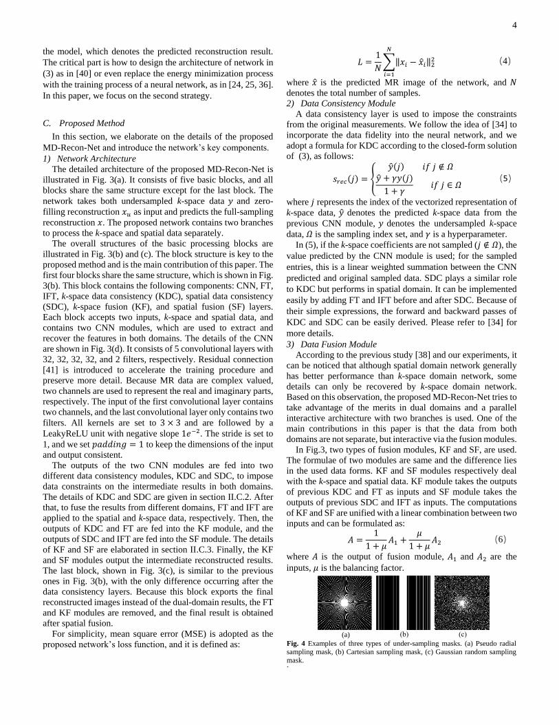
Fig. 4 Examples of three types of under-sampling masks. (a) Pseudo radial
sampling mask, (b) Cartesian sampling mask, (c) Gaussian random sampling
mask.
k
5
III. EXPERIMENTAL DESIGN AND REPRESENTATIVE RESULTS
A. Experimental Simulation Configuration
The public brain MR raw data set—the Calgary-Campinas
dataset1, which comes from a clinical MR scanner (Discovery
MR750; GE Healthcare, Waukesha, WI)—was used to train
and test our proposed model. In total, 4,524 slices from 25
subjects were randomly selected to form the training set, and
the testing set was composed of 1,700 slices from 10 other
subjects. The size of the acquisition matrix is 256 × 256.
Raw MR data are complex valued, but CNNs can only handle
real numbers. There are two common strategies to enable CNNs
to process complex numbers [25]: (a) using two separate
channels to represent the real and imaginary parts, and (b) using
the magnitude of the complex number as the network input. In
this paper, the first strategy was adopted.
The Adam optimizer [42] was used to optimize the network,
and its parameters were set as 𝛼 = 5𝑒−5, 𝛽1 = 0.9, 𝛽2 = 0.999.
The initial learning rate was 5𝑒−5. The parameters 𝛾 in (5) an
d 𝜇 in (6) were trained as network parameters. The PyTorch fr
amework was used for model implementation, and the training
was performed on a graphics processing unit (GTX 1080 Ti).
Our codes for this work are available on https://github.com/De
ep-Imaging-Group/MD-Recon-Net.
For undersampling strategies, three different types of
simulated masks were tested: pseudo radial sampling, Cartesian
sampling, and 2D random sampling (see Fig. 4). For pseudo
radial sampling, 10%, 20%, and 25% sampling rates were tested,
and only a 20% sampling rate was used for the other two types.
To evaluate the performance of the proposed MD-Recon-Net,
its performance was compared with that of five state-of-the-art
methods: DLMRI [21], PANO [43], ADMM-CSNet [30],
DIMENSION [36] and DAGAN [25]. DLMRI2 and PANO3 are
two typical CS-MRI methods based on dictionary learning and
nonlocal means, respectively. ADMM-CSNet 4 is a recently
proposed iteration unrolling method. DAGAN 5 and
DIMENSION are two post-processing network models that
perform on the spatial and dual domains, respectively. All codes
of the compared methods were downloaded from the authors’
websites or implemented strictly according to the original
papers.
To quantitatively evaluate the performance of different
methods, two metrics, peak signal to noise ratio (PSNR) and
structural similarity index measure (SSIM), were employed,
with the following definitions
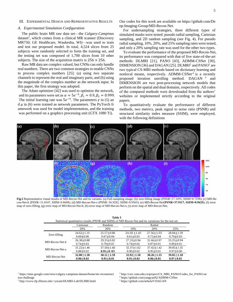
Fig.5 Representative visual results of MD-Recon-Net and its variants. (a) Full-sampling image; (b) zero-filling image (PSNR=27.1055, SSIM=0.7298); (c) MD-Re
con-Net-k (PSNR=31.0347, SSIM=0.8608); (d) MD-Recon-Net-s (PSNR=36.9282, SSIM=0.9565); (e) MD-Recon-Net(PSNR=37.9117, SSIM=0.9625); (f) error
map of zero-filling, (g) error map of MD-Recon-Net-k; (h) error map of MD-Recon-Net-s; (i) error map of MD-Recon-Net;
Table I
Statistical quantitative results (PSNR and SSIM) of MD-Recon-Net and its variations for the test set
Cartesian Random Radial
20% 20% 10% 20% 25%
Zero-filling 24.62±1.35
0.69±0.06
25.57±0.86
0.67±0.04
24.18 ±1.43
0.61±0.05
27.56±1.55
0.75±0.04
28.84±1.59
0.79±0.03
MD-Recon-Net-k 26.38±0.88
0.74±0.03
29.33±0.82
0.79±0.01
27.33±0.94
0.74±0.02
31.66±0.97
0.87±0.01
33.25±0.94
0.90±0.01
MD-Recon-Net-s 31.22±1.46
0.88±0.02
37.50±1.66
0.95±𝟎. 𝟎𝟏
32.37±1.62
0.90±0.02
37.42±1.42
0.95±0.01
39.85±1.35
0.97±0.00
MD-Recon-Net 32.00±1.38
0.90±0.02
38.11±1.59
0.95±0.01
32.92±1.50
0.91±0.02
38.26±1.35
0.96±0.01
39.85±1.18
0.97±0.01
1 https://sites.google.com/view/calgary-campinas-dataset/home/mr-reconstruct
ion-challenge 2 http://www.ifp.illinois.edu/~yoram/DLMRI-Lab/DLMRI.html
3 http://csrc.xmu.edu.cn/project/CS_MRI_PANO/Codes_for_PANO.rar 4 https://github.com/yangyan92/ADMM-CSNet 5 https://github.com/nebulaV/DAGAN
(a) (b) (c)
(d) (e)
(f) (g) (h) (i)
6
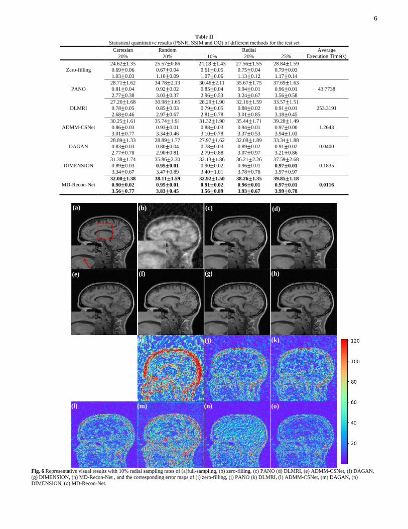
Table II
Statistical quantitative results (PSNR, SSIM and OQ) of different methods for the test set
Cartesian Random Radial Average
Execution Time(s) 20% 20% 10% 20% 25%
Zero-filling
24.62±1.35
0.69±0.06
1.03±0.03
25.57±0.86
0.67±0.04
1.10±0.09
24.18 ±1.43
0.61±0.05
1.07±0.06
27.56±1.55
0.75±0.04
1.13±0.12
28.84±1.59
0.79±0.03
1.17±0.14
PANO
28.71±1.62
0.81±0.04
2.77±0.38
34.78±2.13
0.92±0.02
3.03±0.37
30.46±2.11
0.85±0.04
2.96±0.53
35.67±1.75
0.94±0.01
3.24±0.67
37.69±1.63
0.96±0.01
3.56±0.58
43.7738
DLMRI
27.26±1.68
0.78±0.05
2.68±0.46
30.98±1.65
0.85±0.03
2.97±0.67
28.29±1.90
0.79±0.05
2.81±0.78
32.16±1.59
0.88±0.02
3.01±0.85
33.57±1.51
0.91±0.01
3.18±0.45
253.3191
ADMM-CSNet
30.25±1.61
0.86±0.03
3.01±0.77
35.74±1.91
0.93±0.01
3.34±0.46
31.32±1.90
0.88±0.03
3.10±0.78
35.44±1.71
0.94±0.01
3.37±0.53
39.28±1.49
0.97±0.00
3.94±1.03
1.2643
DAGAN
28.89±1.33
0.83±0.03
2.77±0.78
28.89±1.77
0.80±0.04
2.90±0.81
27.97±1.62
0.78±0.03
2.79±0.88
32.08±1.89
0.89±0.02
3.07±0.97
33.34±1.88
0.91±0.02
3.21±0.86
0.0400
DIMENSION
31.38±1.74
0.89±0.03
3.34±0.67
35.86±2.30
0.95±0.01
3.47±0.89
32.13±1.86
0.90±0.02
3.40±1.01
36.21±2.26
0.96±0.01
3.78±0.78
37.59±2.68
0.97±0.01
3.97±0.97
0.1835
MD-Recon-Net
32.00±1.38
0.90±0.02
3.56±0.77
38.11±1.59
0.95±0.01
3.83±0.45
32.92±1.50
0.91±0.02
3.56±0.89
38.26±1.35
0.96±0.01
3.93±0.67
39.85±1.18
0.97±0.01
3.99±0.78
0.0116
Fig. 6 Representative visual results with 10% radial sampling rates of (a)full-sampling, (b) zero-filling, (c) PANO (d) DLMRI, (e) ADMM-CSNet, (f) DAGAN,
(g) DIMENSION, (h) MD-Recon-Net , and the corresponding error maps of (i) zero-filling, (j) PANO (k) DLMRI, (l) ADMM-CSNet, (m) DAGAN, (n)
DIMENSION, (o) MD-Recon-Net.
(a) (b) (c) (d)
(e) (f) (g) (h)
(i) (j) (k)
(l) (m) (n) (o)
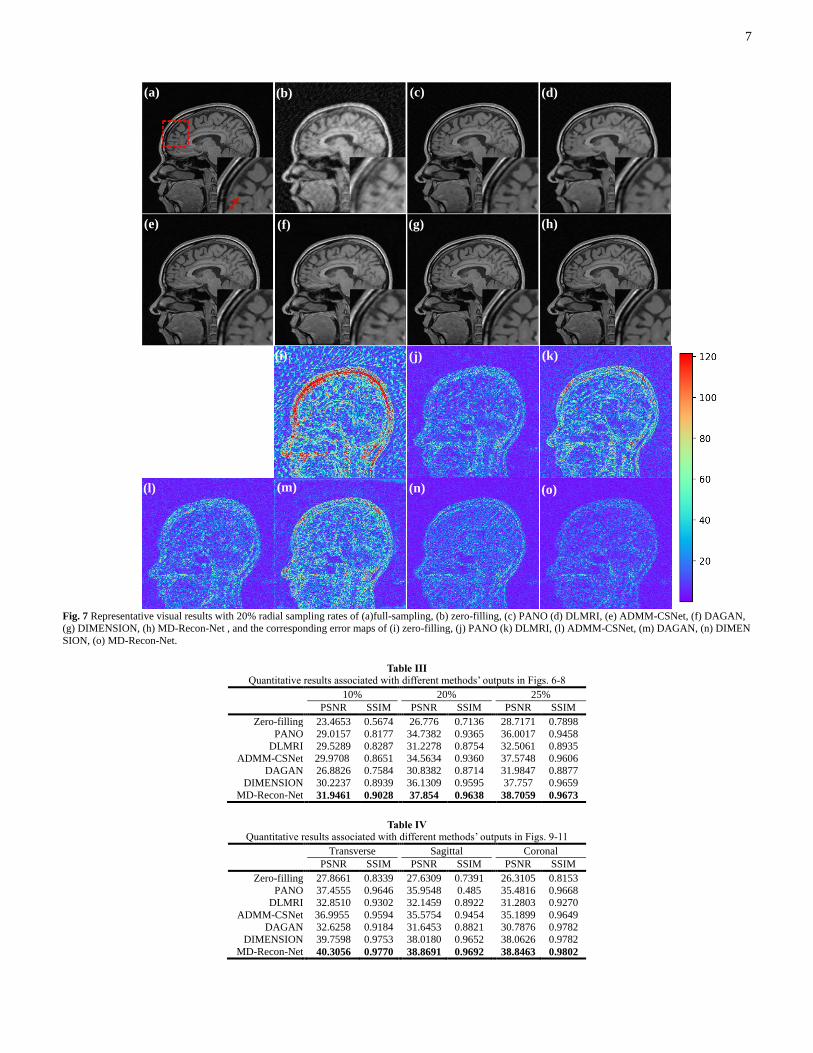
7
Fig. 7 Representative visual results with 20% radial sampling rates of (a)full-sampling, (b) zero-filling, (c) PANO (d) DLMRI, (e) ADMM-CSNet, (f) DAGAN,
(g) DIMENSION, (h) MD-Recon-Net , and the corresponding error maps of (i) zero-filling, (j) PANO (k) DLMRI, (l) ADMM-CSNet, (m) DAGAN, (n) DIMEN
SION, (o) MD-Recon-Net.
Table III
Quantitative results associated with different methods’ outputs in Figs. 6-8
10% 20% 25%
PSNR SSIM PSNR SSIM PSNR SSIM
Zero-filling 23.4653 0.5674 26.776 0.7136 28.7171 0.7898
PANO 29.0157 0.8177 34.7382 0.9365 36.0017 0.9458
DLMRI 29.5289 0.8287 31.2278 0.8754 32.5061 0.8935
ADMM-CSNet 29.9708 0.8651 34.5634 0.9360 37.5748 0.9606
DAGAN 26.8826 0.7584 30.8382 0.8714 31.9847 0.8877
DIMENSION 30.2237 0.8939 36.1309 0.9595 37.757 0.9659
MD-Recon-Net 31.9461 0.9028 37.854 0.9638 38.7059 0.9673
Table IV
Quantitative results associated with different methods’ outputs in Figs. 9-11
Transverse Sagittal Coronal
PSNR SSIM PSNR SSIM PSNR SSIM
Zero-filling 27.8661 0.8339 27.6309 0.7391 26.3105 0.8153
PANO 37.4555 0.9646 35.9548 0.485 35.4816 0.9668
DLMRI 32.8510 0.9302 32.1459 0.8922 31.2803 0.9270
ADMM-CSNet 36.9955 0.9594 35.5754 0.9454 35.1899 0.9649
DAGAN 32.6258 0.9184 31.6453 0.8821 30.7876 0.9782
DIMENSION 39.7598 0.9753 38.0180 0.9652 38.0626 0.9782
MD-Recon-Net 40.3056 0.9770 38.8691 0.9692 38.8463 0.9802
(a) (b) (c) (d)
(e) (f) (g) (h)
(i) (j) (k)
(l) (m) (n) (o)
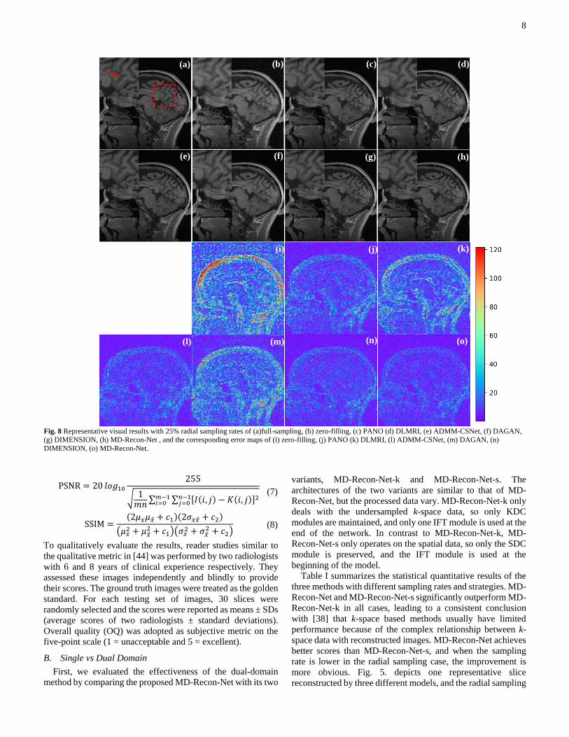
8
Fig. 8 Representative visual results with 25% radial sampling rates of (a)full-sampling, (b) zero-filling, (c) PANO (d) DLMRI, (e) ADMM-CSNet, (f) DAGAN,
(g) DIMENSION, (h) MD-Recon-Net , and the corresponding error maps of (i) zero-filling, (j) PANO (k) DLMRI, (l) ADMM-CSNet, (m) DAGAN, (n)
DIMENSION, (o) MD-Recon-Net.
PSNR = 20 𝑙𝑜𝑔10
255
√ 1𝑚𝑛
∑ ∑ [𝐼(𝑖, 𝑗) − 𝐾(𝑖, 𝑗)]2𝑛−1𝑗=0
𝑚−1𝑖=0
(7)
SSIM =
(2𝜇𝑥𝜇�̂� + 𝑐1)(2𝜎𝑥𝑥 + 𝑐2)
(𝜇𝑥2 + 𝜇�̂�
2 + 𝑐1)(𝜎𝑥2 + 𝜎�̂�
2 + 𝑐2) (8)
To qualitatively evaluate the results, reader studies similar to
the qualitative metric in [44] was performed by two radiologists
with 6 and 8 years of clinical experience respectively. They
assessed these images independently and blindly to provide
their scores. The ground truth images were treated as the golden
standard. For each testing set of images, 30 slices were
randomly selected and the scores were reported as means ± SDs
(average scores of two radiologists ± standard deviations).
Overall quality (OQ) was adopted as subjective metric on the
five-point scale (1 = unacceptable and 5 = excellent).
B. Single vs Dual Domain
First, we evaluated the effectiveness of the dual-domain
method by comparing the proposed MD-Recon-Net with its two
variants, MD-Recon-Net-k and MD-Recon-Net-s. The
architectures of the two variants are similar to that of MD-
Recon-Net, but the processed data vary. MD-Recon-Net-k only
deals with the undersampled k-space data, so only KDC
modules are maintained, and only one IFT module is used at the
end of the network. In contrast to MD-Recon-Net-k, MD-
Recon-Net-s only operates on the spatial data, so only the SDC
module is preserved, and the IFT module is used at the
beginning of the model.
Table I summarizes the statistical quantitative results of the
three methods with different sampling rates and strategies. MD-
Recon-Net and MD-Recon-Net-s significantly outperform MD-
Recon-Net-k in all cases, leading to a consistent conclusion
with [38] that k-space based methods usually have limited
performance because of the complex relationship between k-
space data with reconstructed images. MD-Recon-Net achieves
better scores than MD-Recon-Net-s, and when the sampling
rate is lower in the radial sampling case, the improvement is
more obvious. Fig. 5. depicts one representative slice
reconstructed by three different models, and the radial sampling
(a) (b) (c) (d)
(e) (f) (g) (h)
(i) (j) (k)
(l) (m) (n) (o)
9
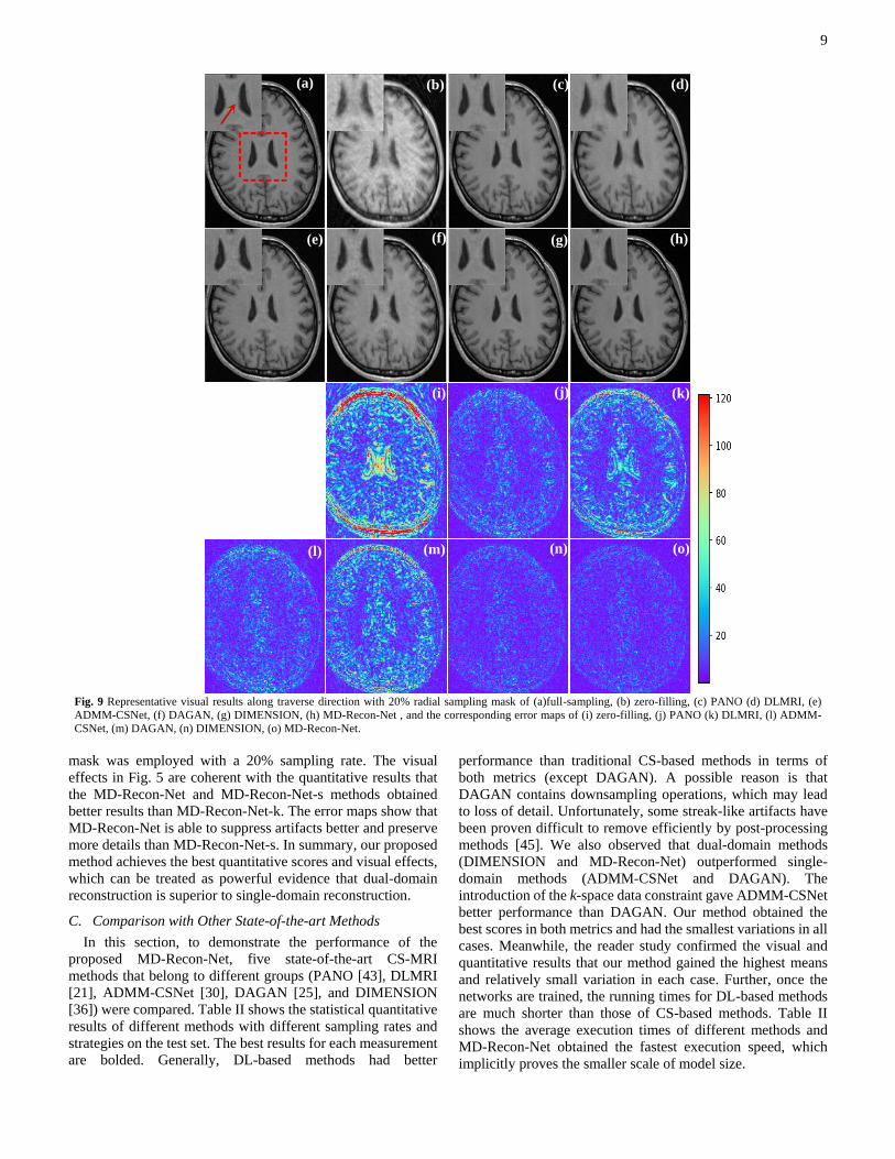
Fig. 9 Representative visual results along traverse direction with 20% radial sampling mask of (a)full-sampling, (b) zero-filling, (c) PANO (d) DLMRI, (e)
ADMM-CSNet, (f) DAGAN, (g) DIMENSION, (h) MD-Recon-Net , and the corresponding error maps of (i) zero-filling, (j) PANO (k) DLMRI, (l) ADMM-
CSNet, (m) DAGAN, (n) DIMENSION, (o) MD-Recon-Net.
mask was employed with a 20% sampling rate. The visual
effects in Fig. 5 are coherent with the quantitative results that
the MD-Recon-Net and MD-Recon-Net-s methods obtained
better results than MD-Recon-Net-k. The error maps show that
MD-Recon-Net is able to suppress artifacts better and preserve
more details than MD-Recon-Net-s. In summary, our proposed
method achieves the best quantitative scores and visual effects,
which can be treated as powerful evidence that dual-domain
reconstruction is superior to single-domain reconstruction.
C. Comparison with Other State-of-the-art Methods
In this section, to demonstrate the performance of the
proposed MD-Recon-Net, five state-of-the-art CS-MRI
methods that belong to different groups (PANO [43], DLMRI
[21], ADMM-CSNet [30], DAGAN [25], and DIMENSION
[36]) were compared. Table II shows the statistical quantitative
results of different methods with different sampling rates and
strategies on the test set. The best results for each measurement
are bolded. Generally, DL-based methods had better
performance than traditional CS-based methods in terms of
both metrics (except DAGAN). A possible reason is that
DAGAN contains downsampling operations, which may lead
to loss of detail. Unfortunately, some streak-like artifacts have
been proven difficult to remove efficiently by post-processing
methods [45]. We also observed that dual-domain methods
(DIMENSION and MD-Recon-Net) outperformed single-
domain methods (ADMM-CSNet and DAGAN). The
introduction of the k-space data constraint gave ADMM-CSNet
better performance than DAGAN. Our method obtained the
best scores in both metrics and had the smallest variations in all
cases. Meanwhile, the reader study confirmed the visual and
quantitative results that our method gained the highest means
and relatively small variation in each case. Further, once the
networks are trained, the running times for DL-based methods
are much shorter than those of CS-based methods. Table II
shows the average execution times of different methods and
MD-Recon-Net obtained the fastest execution speed, which
implicitly proves the smaller scale of model size.
(e) (f) (h)
(i) (j)
(g)
(k)
(l) (m) (n) (o)
(a) (b) (c) (d)
10
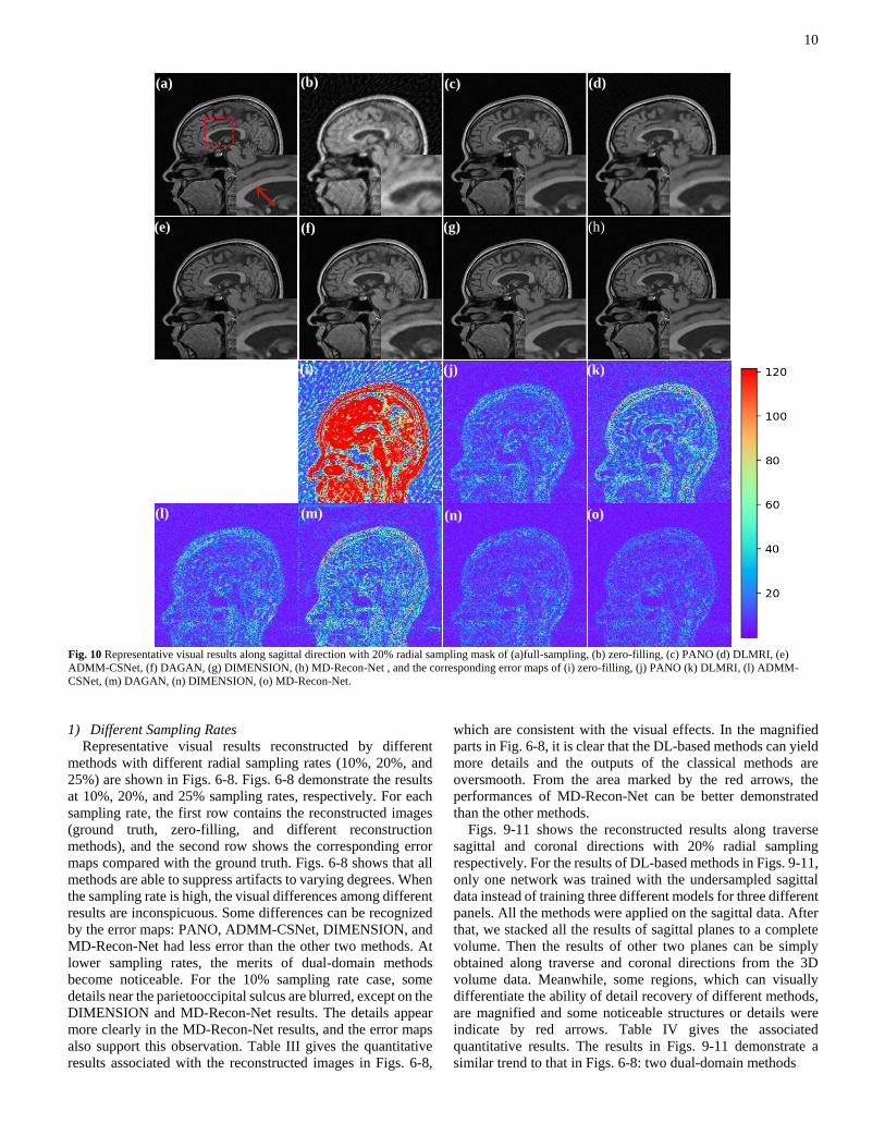
Fig. 10 Representative visual results along sagittal direction with 20% radial sampling mask of (a)full-sampling, (b) zero-filling, (c) PANO (d) DLMRI, (e)
ADMM-CSNet, (f) DAGAN, (g) DIMENSION, (h) MD-Recon-Net , and the corresponding error maps of (i) zero-filling, (j) PANO (k) DLMRI, (l) ADMM-
CSNet, (m) DAGAN, (n) DIMENSION, (o) MD-Recon-Net.
1) Different Sampling Rates
Representative visual results reconstructed by different
methods with different radial sampling rates (10%, 20%, and
25%) are shown in Figs. 6-8. Figs. 6-8 demonstrate the results
at 10%, 20%, and 25% sampling rates, respectively. For each
sampling rate, the first row contains the reconstructed images
(ground truth, zero-filling, and different reconstruction
methods), and the second row shows the corresponding error
maps compared with the ground truth. Figs. 6-8 shows that all
methods are able to suppress artifacts to varying degrees. When
the sampling rate is high, the visual differences among different
results are inconspicuous. Some differences can be recognized
by the error maps: PANO, ADMM-CSNet, DIMENSION, and
MD-Recon-Net had less error than the other two methods. At
lower sampling rates, the merits of dual-domain methods
become noticeable. For the 10% sampling rate case, some
details near the parietooccipital sulcus are blurred, except on the
DIMENSION and MD-Recon-Net results. The details appear
more clearly in the MD-Recon-Net results, and the error maps
also support this observation. Table III gives the quantitative
results associated with the reconstructed images in Figs. 6-8,
which are consistent with the visual effects. In the magnified
parts in Fig. 6-8, it is clear that the DL-based methods can yield
more details and the outputs of the classical methods are
oversmooth. From the area marked by the red arrows, the
performances of MD-Recon-Net can be better demonstrated
than the other methods.
Figs. 9-11 shows the reconstructed results along traverse
sagittal and coronal directions with 20% radial sampling
respectively. For the results of DL-based methods in Figs. 9-11,
only one network was trained with the undersampled sagittal
data instead of training three different models for three different
panels. All the methods were applied on the sagittal data. After
that, we stacked all the results of sagittal planes to a complete
volume. Then the results of other two planes can be simply
obtained along traverse and coronal directions from the 3D
volume data. Meanwhile, some regions, which can visually
differentiate the ability of detail recovery of different methods,
are magnified and some noticeable structures or details were
indicate by red arrows. Table IV gives the associated
quantitative results. The results in Figs. 9-11 demonstrate a
similar trend to that in Figs. 6-8: two dual-domain methods
(a) (b) (c) (d)
(e) (f) (g) (h)
(i) (j) (k)
(l) (m) (n) (o)
11
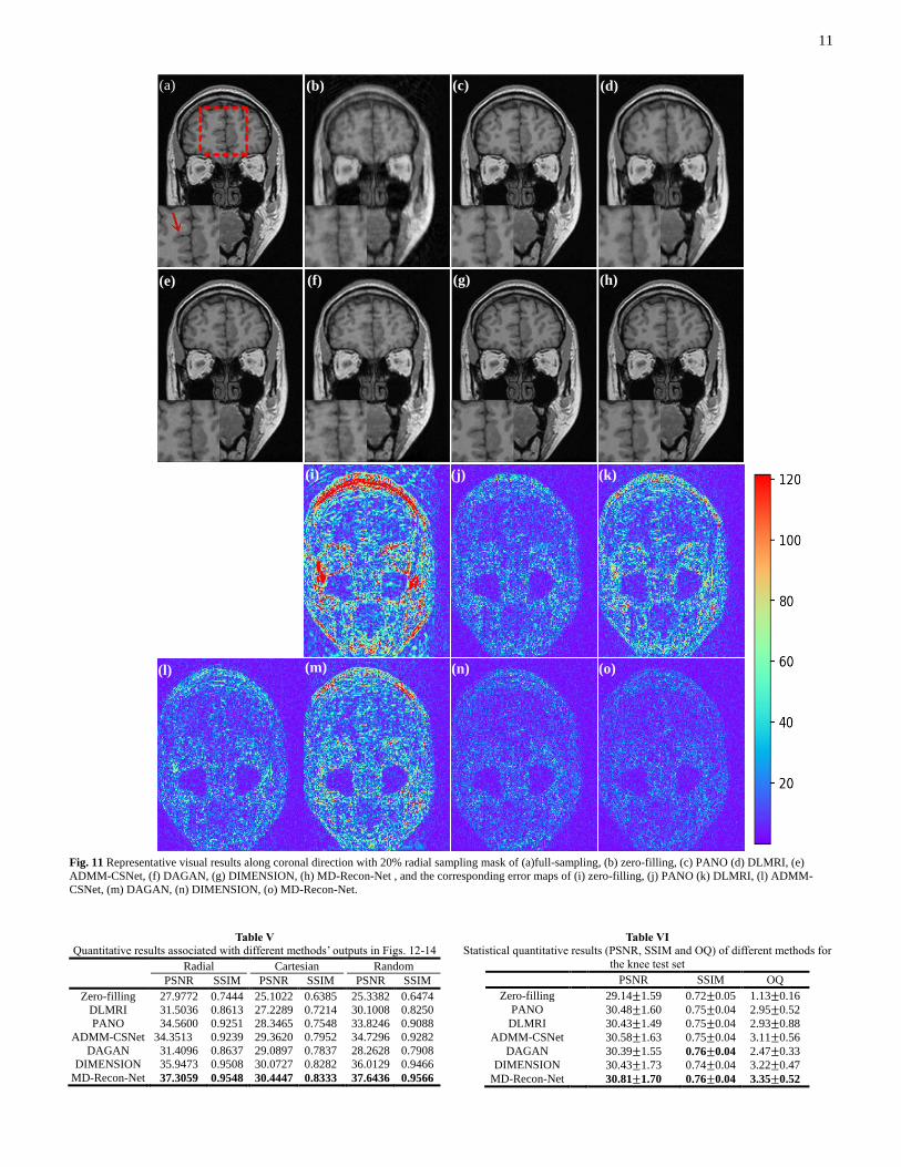
Fig. 11 Representative visual results along coronal direction with 20% radial sampling mask of (a)full-sampling, (b) zero-filling, (c) PANO (d) DLMRI, (e)
ADMM-CSNet, (f) DAGAN, (g) DIMENSION, (h) MD-Recon-Net , and the corresponding error maps of (i) zero-filling, (j) PANO (k) DLMRI, (l) ADMM-
CSNet, (m) DAGAN, (n) DIMENSION, (o) MD-Recon-Net.
Table V
Quantitative results associated with different methods’ outputs in Figs. 12-14
Radial Cartesian Random
PSNR SSIM PSNR SSIM PSNR SSIM
Zero-filling 27.9772 0.7444 25.1022 0.6385 25.3382 0.6474
DLMRI 31.5036 0.8613 27.2289 0.7214 30.1008 0.8250
PANO 34.5600 0.9251 28.3465 0.7548 33.8246 0.9088
ADMM-CSNet 34.3513 0.9239 29.3620 0.7952 34.7296 0.9282
DAGAN 31.4096 0.8637 29.0897 0.7837 28.2628 0.7908
DIMENSION 35.9473 0.9508 30.0727 0.8282 36.0129 0.9466
MD-Recon-Net 37.3059 0.9548 30.4447 0.8333 37.6436 0.9566
Table VI
Statistical quantitative results (PSNR, SSIM and OQ) of different methods for
the knee test set
PSNR SSIM OQ
Zero-filling 29.14±1.59 0.72±0.05 1.13±0.16
PANO 30.48±1.60 0.75±0.04 2.95±0.52
DLMRI 30.43±1.49 0.75±0.04 2.93±0.88
ADMM-CSNet 30.58±1.63 0.75±0.04 3.11±0.56
DAGAN 30.39±1.55 0.76±0.04 2.47±0.33
DIMENSION 30.43±1.73 0.74±0.04 3.22±0.47
MD-Recon-Net 30.81±1.70 0.76±0.04 3.35±0.52
(a) (b) (c) (d)
(e) (f) (g) (h)
(i) (j) (k)
(l) (m) (n) (o)
12
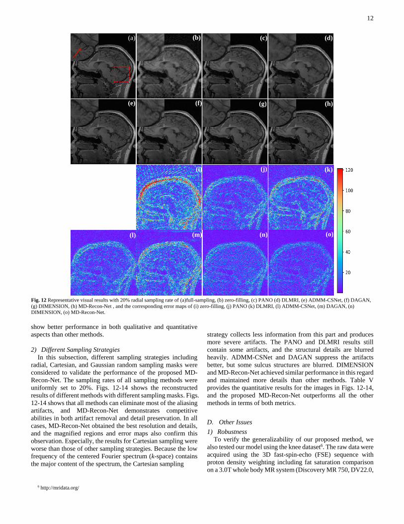
Fig. 12 Representative visual results with 20% radial sampling rate of (a)full-sampling, (b) zero-filling, (c) PANO (d) DLMRI, (e) ADMM-CSNet, (f) DAGAN,
(g) DIMENSION, (h) MD-Recon-Net , and the corresponding error maps of (i) zero-filling, (j) PANO (k) DLMRI, (l) ADMM-CSNet, (m) DAGAN, (n)
DIMENSION, (o) MD-Recon-Net.
show better performance in both qualitative and quantitative
aspects than other methods.
2) Different Sampling Strategies
In this subsection, different sampling strategies including
radial, Cartesian, and Gaussian random sampling masks were
considered to validate the performance of the proposed MD-
Recon-Net. The sampling rates of all sampling methods were
uniformly set to 20%. Figs. 12-14 shows the reconstructed
results of different methods with different sampling masks. Figs.
12-14 shows that all methods can eliminate most of the aliasing
artifacts, and MD-Recon-Net demonstrates competitive
abilities in both artifact removal and detail preservation. In all
cases, MD-Recon-Net obtained the best resolution and details,
and the magnified regions and error maps also confirm this
observation. Especially, the results for Cartesian sampling were
worse than those of other sampling strategies. Because the low
frequency of the centered Fourier spectrum (k-space) contains
the major content of the spectrum, the Cartesian sampling
6 http://mridata.org/
strategy collects less information from this part and produces
more severe artifacts. The PANO and DLMRI results still
contain some artifacts, and the structural details are blurred
heavily. ADMM-CSNet and DAGAN suppress the artifacts
better, but some sulcus structures are blurred. DIMENSION
and MD-Recon-Net achieved similar performance in this regard
and maintained more details than other methods. Table V
provides the quantitative results for the images in Figs. 12-14,
and the proposed MD-Recon-Net outperforms all the other
methods in terms of both metrics.
D. Other Issues
1) Robustness
To verify the generalizability of our proposed method, we
also tested our model using the knee dataset6. The raw data were
acquired using the 3D fast-spin-echo (FSE) sequence with
proton density weighting including fat saturation comparison
on a 3.0T whole body MR system (Discovery MR 750, DV22.0,
(b) (c)
(a) (b) (c) (d)
(e) (f) (g) (h)
(i) (j) (k)
(l) (m) (n) (o)

13
Fig. 13 Representative visual results with 20% cartesian sampling rate of (a)full-sampling, (b) zero-filling, (c) PANO (d) DLMRI, (e) ADMM-CSNet, (f)
DAGAN, (g) DIMENSION, (h) MD-Recon-Net , and the corresponding error maps of (i) zero-filling, (j) PANO (k) DLMRI, (l) ADMM-CSNet, (m) DAGAN,
(n) DIMENSION, (o) MD-Recon-Net.
GE Healthcare, Milwaukee, WI, USA). The repetition time and
echo time were 1,550 ms and 25 ms, respectively. There were
256 slices in total, and each slice’s thickness was 0.6 mm. The
field of view (FOV) was defined as 160×160 mm2, and the size
of acquisition matrix was 320×320. The voxel size was 0.5 mm,
and the number of coils was 8. However, our proposed method
is based on single coil data, so we used a coil compression
algorithm7 to produce single coil k-space data. Table VI shows
the statistical quantitative results of different methods with 20%
sampling rate, and with Cartesian sampling strategy on the
whole set. It can be seen that our MD-Recon-Net obtained the
best scores in both metrics. The results of reader study in Table
VI are coherent with the quantitative results that although the
differences among different methods are smaller than the ones
in previous dataset, the proposed MD-Recon-Net still
performed best in all cases. Fig. 15 shows a representative slice
reconstructed by different methods. DIMENSION and MD-
Recon-Net had the best visual effects. The results from other
7 http://mrsrl.stanford.edu/~tao/software.html
Table VII
Complexity evaluation of different network models
Parameters FLOPs(M)
DAGAN 98600449 2001
DIMENSION 848010 34577
MD-Recon-Net 289319 2106
methods appear slightly blurred, even if the quantitative scores
are close.
2) Model Scale and FLOPs
The complexity of the network model is an important factor
to evaluate the practicability of networks, because it has an
important impact on training difficulty and memory
requirements. Thus, to be fair, we need to compare model
complexity between the available options. In general, the
complexity of deep learning is measured by two metrics: the
amount of parameters (model scale) and floating point
(a) (b) (c) (d)
(e) (f) (g) (h)
(i) (j) (k)
(l) (m) (n) (o)
14
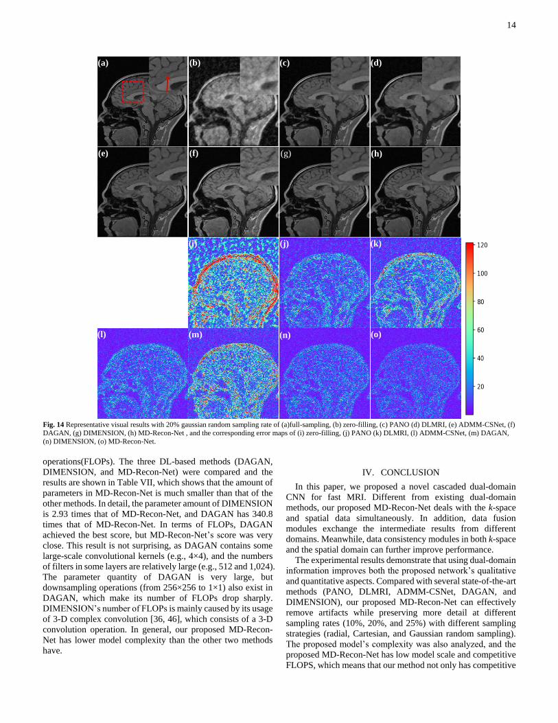
Fig. 14 Representative visual results with 20% gaussian random sampling rate of (a)full-sampling, (b) zero-filling, (c) PANO (d) DLMRI, (e) ADMM-CSNet, (f)
DAGAN, (g) DIMENSION, (h) MD-Recon-Net , and the corresponding error maps of (i) zero-filling, (j) PANO (k) DLMRI, (l) ADMM-CSNet, (m) DAGAN,
(n) DIMENSION, (o) MD-Recon-Net.
operations(FLOPs). The three DL-based methods (DAGAN,
DIMENSION, and MD-Recon-Net) were compared and the
results are shown in Table VII, which shows that the amount of
parameters in MD-Recon-Net is much smaller than that of the
other methods. In detail, the parameter amount of DIMENSION
is 2.93 times that of MD-Recon-Net, and DAGAN has 340.8
times that of MD-Recon-Net. In terms of FLOPs, DAGAN
achieved the best score, but MD-Recon-Net’s score was very
close. This result is not surprising, as DAGAN contains some
large-scale convolutional kernels (e.g., 4×4), and the numbers
of filters in some layers are relatively large (e.g., 512 and 1,024).
The parameter quantity of DAGAN is very large, but
downsampling operations (from 256×256 to 1×1) also exist in
DAGAN, which make its number of FLOPs drop sharply.
DIMENSION’s number of FLOPs is mainly caused by its usage
of 3-D complex convolution [36, 46], which consists of a 3-D
convolution operation. In general, our proposed MD-Recon-
Net has lower model complexity than the other two methods
have.
IV. CONCLUSION
In this paper, we proposed a novel cascaded dual-domain
CNN for fast MRI. Different from existing dual-domain
methods, our proposed MD-Recon-Net deals with the k-space
and spatial data simultaneously. In addition, data fusion
modules exchange the intermediate results from different
domains. Meanwhile, data consistency modules in both k-space
and the spatial domain can further improve performance.
The experimental results demonstrate that using dual-domain
information improves both the proposed network’s qualitative
and quantitative aspects. Compared with several state-of-the-art
methods (PANO, DLMRI, ADMM-CSNet, DAGAN, and
DIMENSION), our proposed MD-Recon-Net can effectively
remove artifacts while preserving more detail at different
sampling rates (10%, 20%, and 25%) with different sampling
strategies (radial, Cartesian, and Gaussian random sampling).
The proposed model’s complexity was also analyzed, and the
proposed MD-Recon-Net has low model scale and competitive
FLOPS, which means that our method not only has competitive
(a) (b) (c) (d)
(e) (f) (g) (h)
(i) (j) (k)
(l) (m) (n) (o)
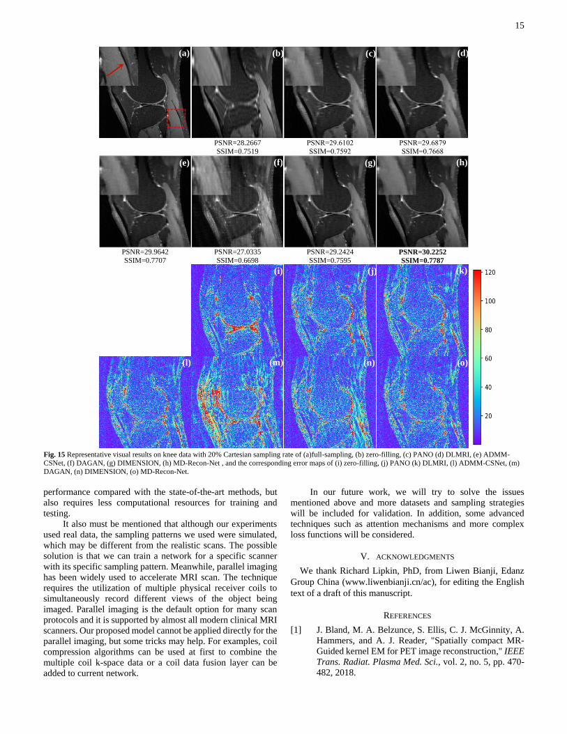
15
PSNR=28.2667
SSIM=0.7519 PSNR=29.6102 SSIM=0.7592
PSNR=29.6879 SSIM=0.7668
PSNR=29.9642 SSIM=0.7707
PSNR=27.0335 SSIM=0.6698
PSNR=29.2424 SSIM=0.7595
PSNR=30.2252 SSIM=0.7787
Fig. 15 Representative visual results on knee data with 20% Cartesian sampling rate of (a)full-sampling, (b) zero-filling, (c) PANO (d) DLMRI, (e) ADMM-
CSNet, (f) DAGAN, (g) DIMENSION, (h) MD-Recon-Net , and the corresponding error maps of (i) zero-filling, (j) PANO (k) DLMRI, (l) ADMM-CSNet, (m)
DAGAN, (n) DIMENSION, (o) MD-Recon-Net.
performance compared with the state-of-the-art methods, but
also requires less computational resources for training and
testing.
It also must be mentioned that although our experiments
used real data, the sampling patterns we used were simulated,
which may be different from the realistic scans. The possible
solution is that we can train a network for a specific scanner
with its specific sampling pattern. Meanwhile, parallel imaging
has been widely used to accelerate MRI scan. The technique
requires the utilization of multiple physical receiver coils to
simultaneously record different views of the object being
imaged. Parallel imaging is the default option for many scan
protocols and it is supported by almost all modern clinical MRI
scanners. Our proposed model cannot be applied directly for the
parallel imaging, but some tricks may help. For examples, coil
compression algorithms can be used at first to combine the
multiple coil k-space data or a coil data fusion layer can be
added to current network.
In our future work, we will try to solve the issues
mentioned above and more datasets and sampling strategies
will be included for validation. In addition, some advanced
techniques such as attention mechanisms and more complex
loss functions will be considered.
V. ACKNOWLEDGMENTS
We thank Richard Lipkin, PhD, from Liwen Bianji, Edanz
Group China (www.liwenbianji.cn/ac), for editing the English
text of a draft of this manuscript.
REFERENCES
[1] J. Bland, M. A. Belzunce, S. Ellis, C. J. McGinnity, A.
Hammers, and A. J. Reader, "Spatially compact MR-
Guided kernel EM for PET image reconstruction," IEEE
Trans. Radiat. Plasma Med. Sci., vol. 2, no. 5, pp. 470-
482, 2018.
(a) (b) (c) (d)
(e) (f) (g) (h)
(i) (j) (k)
(l) (m) (n) (o)
16
[2] J. Bland et al., "MR-guided kernel EM reconstruction
for reduced dose PET imaging," IEEE Trans. Radiat.
Plasma Med. Sci., vol. 2, no. 3, pp. 235-243, 2017.
[3] K. M. Ropella-Panagis, N. Seiberlich, and V. Gulani,
"Magnetic resonance fingerprinting: Implications and
opportunities for PET/MR," IEEE Trans. Radiat.
Plasma Med. Sci., vol. 3, no. 4, pp. 388-399, 2019.
[4] J. Hamilton, D. Franson, and N. Seiberlich, "Recent
advances in parallel imaging for MRI," Prog. Nucl.
Magn. Reson. Spectrosc., vol. 101, pp. 71-95, 2017.
[5] P. B. Roemer, W. A. Edelstein, C. E. Hayes, S. P. Souza,
and O. M. Mueller, "The NMR phased array," Magn.
Reson. Med., vol. 16, no. 2, pp. 192-225, 1990.
[6] K. P. Pruessmann, M. Weiger, P. Börnert, and P.
Boesiger, "Advances in sensitivity encoding with
arbitrary k‐space trajectories," Magn. Reson. Med., vol.
46, no. 4, pp. 638-651, 2001.
[7] K. P. Pruessmann, M. Weiger, M. B. Scheidegger, and
P. Boesiger, "SENSE: sensitivity encoding for fast
MRI," Magn. Reson. Med., vol. 42, no. 5, pp. 952-962,
1999.
[8] D. Liang, B. Liu, J. Wang, and L. Ying, "Accelerating
SENSE using compressed sensing," Magn. Reson. Med.,
vol. 62, no. 6, pp. 1574-1584, 2009.
[9] P. Kellman, F. H. Epstein, and E. R. McVeigh,
"Adaptive sensitivity encoding incorporating temporal
filtering (TSENSE)," Magn. Reson. Med., vol. 45, no. 5,
pp. 846-852, 2001.
[10] Y. J. Ma, W. Liu, X. Tang, and J. H. Gao, "Improved
SENSE imaging using accurate coil sensitivity maps
generated by a global magnitude‐phase fitting method,"
Magn. Reson. Med., vol. 74, no. 1, pp. 217-224, 2015.
[11] J. Wang, T. Kluge, M. Nittka, V. Jellus, B. Kuehn, and
B. Kiefer, "Parallel acquisition techniques with modified
SENSE reconstruction mSENSE," in Proceedings of the
First Würzburg Workshop on Parallel Imaging Basics
and Clinical Applications, 2001, p. 89.
[12] C. A. McKenzie, M. A. Ohliger, E. N. Yeh, M. D. Price,
and D. K. Sodickson, "Coil ‐ by ‐ coil image
reconstruction with SMASH," Magn. Reson. Med., vol.
46, no. 3, pp. 619-623, 2001.
[13] M. Bydder, D. J. Larkman, and J. V. Hajnal,
"Generalized SMASH imaging," Magn. Reson. Med.,
vol. 47, no. 1, pp. 160-170, 2002.
[14] D. K. Sodickson, "Simultaneous acquisition of spatial
harmonics (SMASH): ultra-fast imaging with
radiofrequency coil arrays," ed: Google Patents, 1999.
[15] M. A. Griswold et al., "Generalized autocalibrating
partially parallel acquisitions (GRAPPA)," Magn. Reson.
Med., vol. 47, no. 6, pp. 1202-1210, 2002.
[16] W. E. Kyriakos et al., "Sensitivity profiles from an array
of coils for encoding and reconstruction in parallel
(SPACE RIP)," Magn. Reson. Med., vol. 44, no. 2, pp.
301-308, 2000.
[17] M. Lustig and J. M. Pauly, "SPIRiT: iterative self‐
consistent parallel imaging reconstruction from arbitrary
k‐space," Magn. Reson. Med., vol. 64, no. 2, pp. 457-
471, 2010.
[18] D. L. Donoho, "Compressed sensing," IEEE Trans. Inf.
Theory, vol. 52, no. 4, pp. 1289-1306, 2006.
[19] M. Lustig, D. L. Donoho, J. M. Santos, and J. M. Pauly,
"Compressed sensing MRI," IEEE signal processing
magazine, vol. 25, no. 2, p. 72, 2008.
[20] M. Lustig, D. Donoho, and J. M. Pauly, "Sparse MRI:
The application of compressed sensing for rapid MR
imaging," Magn. Reson. Med., vol. 58, no. 6, pp. 1182-
1195, 2007.
[21] S. Ravishankar and Y. Bresler, "MR image
reconstruction from highly undersampled k-space data
by dictionary learning," IEEE Trans. Med. Imaging, vol.
30, no. 5, pp. 1028-1041, 2010.
[22] J. Caballero, A. N. Price, D. Rueckert, and J. V. Hajnal,
"Dictionary learning and time sparsity for dynamic MR
data reconstruction," IEEE Trans. Med. Imaging, vol. 33,
no. 4, pp. 979-994, 2014.
[23] S. Ravishankar and Y. Bresler, "Sparsifying transform
learning for compressed sensing MRI," in Proc. IEEE
13th Int. Symp. Biomed. Imag.(ISBI), 2013, pp. 17-20.
[24] T. M. Quan, T. Nguyen-Duc, and W.-K. Jeong,
"Compressed sensing MRI reconstruction using a
generative adversarial network with a cyclic loss," IEEE
Trans. Med. Imaging, vol. 37, no. 6, pp. 1488-1497,
2018.
[25] G. Yang et al., "DAGAN: deep de-aliasing generative
adversarial networks for fast compressed sensing MRI
reconstruction," IEEE Trans. Med. Imaging, vol. 37, no.
6, pp. 1310-1321, 2017.
[26] Y. Han, J. Yoo, H. H. Kim, H. J. Shin, K. Sung, and J.
C. Ye, "Deep learning with domain adaptation for
accelerated projection ‐ reconstruction MR," Magn.
Reson. Med., vol. 80, no. 3, pp. 1189-1205, 2018.
[27] D. Lee, J. Yoo, S. Tak, and J. C. Ye, "Deep residual
learning for accelerated MRI using magnitude and phase
networks," IEEE Trans. Biomed. Eng., vol. 65, no. 9, pp.
1985-1995, 2018.
[28] M. Mardani et al., "Deep generative adversarial neural
networks for compressive sensing MRI," IEEE Trans.
Med. Imaging, vol. 38, no. 1, pp. 167-179, 2018.
[29] Y. Han, L. Sunwoo, and J. C. Ye, "k-space deep learning
for accelerated MRI," IEEE Trans. Med. Imaging, 2019.
[30] Y. Yang, J. Sun, H. Li, and Z. Xu, "ADMM-CSNet: A
Deep Learning Approach for Image Compressive
Sensing," IEEE Trans. Pattern Anal. Mach. Intell., 2018.
[31] C. Qin, J. Schlemper, J. Caballero, A. N. Price, J. V.
Hajnal, and D. Rueckert, "Convolutional recurrent
neural networks for dynamic MR image reconstruction,"
IEEE Trans. Med. Imaging, vol. 38, no. 1, pp. 280-290,
2018.
[32] H. K. Aggarwal, M. P. Mani, and M. Jacob, "Modl:
Model-based deep learning architecture for inverse
problems," IEEE Trans. Med. Imaging, vol. 38, no. 2, pp.
394-405, 2018.
[33] J. Schlemper et al., "Stochastic deep compressive
sensing for the reconstruction of diffusion tensor cardiac
MRI," in International conference on medical image
computing and computer-assisted intervention, 2018:
Springer, pp. 295-303.
17
[34] J. Schlemper, J. Caballero, J. V. Hajnal, A. N. Price, and
D. Rueckert, "A deep cascade of convolutional neural
networks for dynamic MR image reconstruction," IEEE
Trans. Med. Imaging, vol. 37, no. 2, pp. 491-503, 2017.
[35] B. Zhu, J. Z. Liu, S. F. Cauley, B. R. Rosen, and M. S.
Rosen, "Image reconstruction by domain-transform
manifold learning," Nature, vol. 555, no. 7697, p. 487,
2018.
[36] S. Wang et al., "DIMENSION: Dynamic MR imaging
with both k-space and spatial prior knowledge obtained
via multi-supervised network training," NMR Biomed.,
2018.
[37] R. Souza, R. M. Lebel, and R. Frayne, "A Hybrid, Dual
Domain, Cascade of Convolutional Neural Networks for
Magnetic Resonance Image Reconstruction,"
Proceedings of Machine Learning vol. 1, p. 11, 2019.
[38] T. Eo, Y. Jun, T. Kim, J. Jang, H. J. Lee, and D. Hwang,
"KIKI ‐ net: cross ‐ domain convolutional neural
networks for reconstructing undersampled magnetic
resonance images," Magn. Reson. Med., vol. 80, no. 5,
pp. 2188-2201, 2018.
[39] K. Hammernik et al., "Learning a variational network
for reconstruction of accelerated MRI data," Magn.
Reson. Med., vol. 79, no. 6, pp. 3055-3071, 2018.
[40] S. Wang et al., "Accelerating magnetic resonance
imaging via deep learning," in Proc. IEEE 13th Int.
Symp. Biomed. Imag.(ISBI), 2016, pp. 514-517.
[41] K. He, X. Zhang, S. Ren, and J. Sun, "Deep residual
learning for image recognition," in Proceedings of the
IEEE conference on computer vision and pattern
recognition(CVPR), 2016, pp. 770-778.
[42] D. Kinga and J. B. Adam, "Adam: A method for
stochastic optimization," in Proc. Int. Conf. Learning
Representations (ICLR), 2015, vol. 5.
[43] X. Qu, Y. Hou, F. Lam, D. Guo, J. Zhong, and Z. Chen,
"Magnetic resonance image reconstruction from
undersampled measurements using a patch-based
nonlocal operator," Med. Image Anal., vol. 18, no. 6, pp.
843-856, 2014.
[44] M. Seitzer et al., "Adversarial and perceptual refinement
for compressed sensing MRI reconstruction," in Int.
Conf. Med. Image Comput. Comput. Assist.
Interv.(MICCAI), 2018: Springer, pp. 232-240.
[45] H. Chen et al., "LEARN: Learned experts’ assessment-
based reconstruction network for sparse-data CT," IEEE
Trans. Med. Imaging, vol. 37, no. 6, pp. 1333-1347,
2018.
[46] C. Trabelsi et al., "Deep complex networks," arXiv
preprint arXiv:1705.09792, 2017.