Linear Algebra and its Applications 429 (2008) 1191–1212

Available online at www.sciencedirect.com

www.elsevier.com/locate/laa

Linear system modelization of concatenated blockand convolutional codes�

Joan-Josep Climent a ,∗, Victoria Herranz b, Carmen Perea b

a Institut Universitari d’Investigacio Informatica, Departament de Ciencia de la Computacio i Intel·ligencia Artificial,Universitat d’Alacant, Campus de Sant Vicent del Raspeig, Ap. Correus 99, E-03080 Alacant, Spain

b Centro de Investigacion Operativa, Departamento de Estadıstica, Matematicas e Informatica,Universidad Miguel Hernandez, Avda. Universidad s/n, E-03202 Elche, Spain

Received 30 October 2006; accepted 11 September 2007Available online 29 October 2007

Submitted by P. Van Dooren

Abstract

In this paper, we characterize four models of concatenation of a block code and a convolutional codefrom a linear systems theory viewpoint. We provide the input-state-output representation of these modelsand we give conditions in order to get a non-catastrophic concatenated convolutional code with minimalrepresentation. Lower bounds on the free distances of the concatenated codes are also developed.© 2007 Elsevier Inc. All rights reserved.

Keywords: Concatenated code; Input-state-output representation; Minimal representation; Observable pair; Controllablepair; Column distance; Free distance; MDS code; Strongly MDS convolutional code

1. Introduction

The major difficulty of using coding for transmission is that, in an effort to approach thetheoretical limit for Shannon’s channel capacity, there is a need to increase the codeword lengthof a linear block code or a constraint length of a convolutional code, which, in turn, causes thecomputational complexity of a decoder to increase exponentially. The way to solve the problem is

� This work was partially supported by Spanish Grant MTM2005-05759. The work of the second and third authorswere also supported by Spanish regional Grants SA028A05 and E-GV06/078.

∗ Corresponding author. Tel.: +34 96 590 3655; fax: +34 96 590 3902.E-mail address: jcliment@ua.es (J.-J. Climent).

0024-3795/$ - see front matter ( 2007 Elsevier Inc. All rights reserved.doi:10.1016/j.laa.2007.09.006

1192 J.-J. Climent et al. / Linear Algebra and its Applications 429 (2008) 1191–1212

to use a concatenated code, where two (or more) constituent codes are used in serial or in parallel.For example, further enhancements to GSM networks are provided by Enhanced Data rates forGSM Evolution (EDGE) technology, in which a Forney scheme of concatenation is used, withouter q-ary Reed–Solomon code and inner binary convolutional code.

Nevertheless, our goal in this paper is to give a mathematical approximation of differentconcatenations of a block and a convolutional code, over any field, in order to characterize theseconcatenations and provide lower bounds on the free distances.

According to the Shannon theory, most codes are good provided that they are long enough[22]. However, decoding complexity is also known to increase with the code length. Concatenatedcodes were introduced by Forney [8] as a way of providing long codes with manageable decodingcomplexity, through a cascade of an outer block code and an inner convolutional code. Otherauthors introduced the concatenation of two convolutional codes [10]. During the last decades,some types of concatenation have appeared, such as the well-known turbo codes [3–5,17] andthe alternative concatenations of them have been studied [1,2]. More recently, Höst et al. [13]developed woven convolutional codes as a combination of serial and parallel concatenation ofconvolutional codes. The characteristics of these codes were further investigated in [9,14,16].Turbo codes have many applications, starting from data storage systems through to wire-line andwireless communications (used in digital video broadcasting, satellite communications, spaceexploring systems, and implementation technologies). Although turbo codes and woven convolu-tional codes use an interleaver, this does not affect the results of either the concatenation propertiesor the lower bounds on the free distance which we analyze in this paper.

Some types of concatenated codes have been studied using the generator matrix. Nevertheless,Climent et al. [6,7], presented a characterization of two kinds of concatenation of convolutionalcodes from a linear systems theory viewpoint.

The paper is structured as follows. Our starting point in Section 2 will be the linear systemsrepresentation of convolutional codes; we present some recent advances in this area. Using someclassical ideas from linear systems theory, we introduce the concatenation of a block code anda convolutional code in Section 3. In Section 4 we give the conditions for getting a minimalinput-state-output realization of the different models of concatenation. In Section 5 we give someresults on the column distances and free distances of the concatenated codes; in addition, wedevelop some conditions in order to obtain a strongly MDS convolutional code for two typesof concatenation. Finally, in Section 6 we give some relations between the differents models ofconcatenation.

2. Preliminary results

Throughout the paper, we denote by F = GF(q) the Galois field of q elements and F thealgebraic closure of F.

Error correcting codes are usually divided in two distinct classes: block codes and convolutionalcodes. A block code is the primary type of channel coding which was used in earlier mobilecommunication systems.

A block code B can be characterized as the set of codewords v ∈ Fn so that v = Gu for anyinformation vector u ∈ Fk (with k ∈ N), where G is an n × k matrix of full column rank called

a generator matrix of B. In addition, if G =(

IkP

), is said to be systematic. Observe that the

systematicity of the generator matrix is only a property of the generator matrix, but not a propertyof the code. We refer to B as an [n, k]-code. The dual of B is the code

J.-J. Climent et al. / Linear Algebra and its Applications 429 (2008) 1191–1212 1193

B⊥ = {v ∈ Fn|GTv = 0}.The Hamming weight wt(v) of a vector v ∈ Fn is the number of its nonzero components; theminimum distance of B is then defined as

dmin(B) = min{wt(v)|v ∈ B with v /= 0},and the code B can correct up to

⌊dmin(B)−1

2

⌋errors. So, we must consider a block code with as

large minimum distance as possible.A natural upper bound on the minimum distance of an [n, k]-code is given by the Singleton

bound

dmin(B) � n − k + 1.

A block code which attains this upper bound is called a maximum distance separable (MDS)block code, and it can be characterized in terms of its systematic generator matrix.

Theorem 1 (Theorem 5.3.7 of [18]). LetB be an [n, k]-code over F, then the following statementsare equivalent:

(a) B is an MDS block code.

(b) If G =(

IkP

)is a systematic generator matrix for B, then every square submatrix of P is

nonsingular.

On the other hand, a convolutional code C of rate k/n and degree δ, called an (n, k, δ)-code,can be given by the input-state-output representation (see [15,19,21])

xt+1 = Axt + But ,

yt = Cxt + Dut ,

vt =(

yt

ut

), x0 = 0,

(1)

where for each instant t , xt ∈ Fδ is the state vector, ut ∈ Fk is the information vector, yt ∈ Fn−k isthe parity vector and vt is a codeword of C. In that case, C is said to be generated by (A, B, C, D)

and by abuse of notation we denote it by C(A, B, C, D).Here A, B, C and D are matrices of sizes δ × δ, δ × k, (n − k) × δ and (n − k) × k, respec-

tively, that is, (A, B, C, D) is a minimal representation and it is characterized through the conditionthat the pair (A, B) is controllable, i.e.,

rank(B AB · · · Aδ−1B) = δ

or equivalently (see [11]),

rank(zI − A B) = δ, for all z ∈ F

(A, C) is said to be an observable pair if (AT, CT) is a controllable pair, i.e.,

rank

⎛⎜⎜⎜⎝C

CA...

CAδ−1

⎞⎟⎟⎟⎠ = δ

1194 J.-J. Climent et al. / Linear Algebra and its Applications 429 (2008) 1191–1212

or equivalently (see [11]),

rank

(zI − A

C

)= δ, for all z ∈ F.

We define a convolutional code C(A, B, C, D) to be observable if one and therefore everyencoder G(z) is right prime. If G(z) is an encoder of an observable convolutional code, thenG(z) is necessarily a non-catastrophic encoder. The following result shows that if (A, B) iscontrollable, then the observability of the pair (A, C) ensures that the linear system (1) describesa non-catastrophic convolutional encoder.

Lemma 2 (Lemma 2.11 of [21]). Assume that the matrices (A, B) form a controllable pair. Theconvolutional code C(A, B, C, D) defined through (1) represents an observable convolutionalcode if and only if (A, C) forms an observable pair.

Finally, in terms of the input-state-output representation (1), the free distance of a convolutionalcode C, that is, the minimum Hamming distances between any two code sequences of C, can becharacterized as (see [15])

dfree(C) = limj→∞ dc

j (C), (2)

where

dcj (C) = min

u0 /=0

⎧⎨⎩j∑

t=0

wt(ut ) +j∑

t=0

wt(yt )

⎫⎬⎭ (3)

is the j th column distance of the convolutional code C, for j = 0, 1, 2, . . ..For algebraic reasons we assume that vt in Eq. (1) is a finite-weight codeword (see [21]), i.e.,

Eq. (1) is satisfied for all t = 0, 1, 2, . . . and there is an integer γ such that xt+1 = 0, ut = 0, andtherefore yt = 0, for t � γ + 1, which is equivalent (see [21, Proposition 2.4]) to

(O Aγ B Aγ−1B · · · AB B

−I Tγ

)⎛⎜⎜⎜⎜⎜⎜⎜⎜⎜⎜⎜⎜⎝

y0y1...

yγ

u0u1...

uγ

⎞⎟⎟⎟⎟⎟⎟⎟⎟⎟⎟⎟⎟⎠= O, (4)

where

Tγ =

⎛⎜⎜⎜⎜⎜⎜⎝

D

CB D

CAB CB. . .

......

. . .CAγ−1B CAγ−2B · · · CB D

⎞⎟⎟⎟⎟⎟⎟⎠ .

Here and in the rest of the paper, we denote by O the zero matrix of the appropriate size.The free distance of an (n, k, δ)-code C is upper-bounded (see [20]) by the generalized Sin-

gleton bound

J.-J. Climent et al. / Linear Algebra and its Applications 429 (2008) 1191–1212 1195

dfree(C) � (n − k)

(⌊δ

k

⌋+ 1

)+ δ + 1

and C is said to be a maximum distance separable (MDS) code if its free distance attains thegeneralized bound. Furthermore, C is said to have maximum distance profile (see [15]) if

dcj (C) = (n − k)(j + 1) + 1 for j = 0, 1, . . . , L where L =

⌊δ

k

⌋+

⌊δ

n − k

⌋.

Finally, C is said to be a strongly MDS code (see [15]) if

dcM(C) = (n − k)

(⌊δ

k

⌋+ 1

)+ δ + 1 for M =

⌊δ

k

⌋+

⌈δ

n − k

⌉.

Clearly, a strongly MDS code is an MDS code.

Remark 3. Observe that if n − k divides δ, then M = L and a convolutional code C has amaximum distance profile if and only if C is strongly MDS.

To finish this section, we quote the following result due to Hutchinson et al. [15], for furtherreferences.

Theorem 4 (Corollary 2.5 of [15]). Let L = ⌊δk

⌋ +⌊

δn−k

⌋. Then, the matrices (A, B, C, D)

generate a maximum distance profile (n, k, δ)-code if and only if the matrix TL has the propertythat every minor which is non trivially zero is nonzero.

3. Models of concatenation of a block code and a convolutional code

In this section we introduce four models of concatenation of a block code and a convolutionalcode. These models are studied in order to provide, from a perspective of mathematical theory,strongly MDS convolutional codes from the concatenation of a block and convolutional codewhich are not necessarily MDS codes. Let Co be a block code, called outer code, and let Ci be aconvolutional code, called inner code. Let u

(1)t be the information vector of Co, and let x

(2)t , u(2)

t ,and y

(2)t be the state vector, the information vector and the parity vector of Ci , respectively.

3.1. First model

In the first model of concatenation, the outer code Co and the inner code Ci are serialized,one after the other (see Fig. 1), so that the input information u

(1)t is fed to Co and the obtained

codeword

Fig. 1. Concatenated code BC(1).

1196 J.-J. Climent et al. / Linear Algebra and its Applications 429 (2008) 1191–1212

v(1)t = Gu

(1)t (5)

is then encoded by Ci in a way that

u(2)t = v

(1)t . (6)

So, the codewords v(2)t of Ci are given by

v(2)t =

(y

(2)t

u(2)t

). (7)

We denote by BC(1) the corresponding concatenated convolutional code. Observe that the vectorstate xt , the information vector ut and the parity vector yt of BC(1) are given by

xt = x(2)t , ut = u

(1)t , and yt = y

(2)t . (8)

So the codewords vt of BC(1) are given by

vt =(

yt

ut

)=

(y

(2)t

u(1)t

). (9)

The next theorem introduces the input-state-output representation of the concatenated convo-lutional code BC(1) from the generator matrix of the outer code Co and the input-state-outputrepresentation of the inner code Ci .

Theorem 5. Let Co be an [m, k]-code with generator matrix G and let Ci (A2, B2, C2, D2) be an(n + m − k, m, δ)-code. Then the input-state-output representation for the rate k/n concatenatedcode BC(1) is given by system (1), with

A = A2, B = B2G, C = C2, and D = D2G. (10)

Proof. From expression (1) we have, for the code Ci ,

x(2)t+1 = A2x

(2)t + B2u

(2)t ,

y(2)t = C2x

(2)t + D2u

(2)t .

Now, taking into account expressions (5)–(8), the input-state-output representation of the concat-enated code BC(1) is given by

xt+1 = A2xt + B2Gut ,

yt = C2xt + D2Gut . �

3.2. Second model

If in the first model we consider that the generator matrix G of the block codeCo is in systematic

form, that is, G =(

IkP

)and we consider the parity check vector Pu

(1)t of the obtained codeword

v(1)t =

(u

(1)t

P u(1)t

)(11)

J.-J. Climent et al. / Linear Algebra and its Applications 429 (2008) 1191–1212 1197

Fig. 2. Concatenated code BC(1)sys.

of Co as the input of Ci , that is,

u(2)t = Pu

(1)t , (12)

then we obtain the concatenated code of Fig. 2. Here the codewords v(2)t of Ci are given by

v(2)t =

(y

(2)t

u(2)t

). (13)

We denote by BC(1)sys the corresponding concatenated convolutional code.

Analogously to the modelBC(1), the vector state xt , the information vector ut , the parity vectoryt and the codewords vt of BC

(1)sys are given by expressions (8) and (9). The input-state-output

representation of the concatenated code BC(1)sys is given by the following theorem whose proof is

similar to that of Theorem 5 and is omitted.

Theorem 6. LetCo be an [m, k]-code with generator matrixG =(

IkP

)and letCi (A2, B2, C2, D2)

be an (n + m − 2k, m − k, δ)-code. Then the input-state-output representation for the rate k/n

concatenated code BC(1)sys is given by system (1), with

A = A2, B = B2P, C = C2, and D = D2P. (14)

3.3. Third model

If we vary the codeBC(1) so that the codeword v(1)t of the outer code is a part of the concatenated

codeword (see Fig. 3), we obtain a new concatenated convolutional code that we denote byBC(2). Here, the information vector u

(1)t and the codeword v

(1)t of Co and the information vector

u(2)t and the codewords v

(2)t of Ci are the same as in the first model (see expressions (5)–(7)).

Then, the vector state xt , the information vector ut and the parity vector yt of BC(2) are givenby

Fig. 3. Concatenated code BC(2).

1198 J.-J. Climent et al. / Linear Algebra and its Applications 429 (2008) 1191–1212

xt = x(2)t , ut = u

(1)t , and yt =

(y

(2)t

v(1)t

)=

(y

(2)t

Gu(1)t

)(15)

and the codewords vt of BC(2) are given by

vt =(

yt

ut

)=

⎛⎜⎝ y(2)t

Gu(1)t

u(1)t

⎞⎟⎠ .

The next theorem, whose proof is similar to that of Theorem 5, provides the input-state-outputrepresentation of the convolutional code BC(2) from the generator matrix of the outer code Co

and the input-state-output representation of the inner code Ci .

Theorem 7. Let Co be an [m, k]-code with generator matrix G and let Ci (A2, B2, C2, D2) bean (n − k, m, δ)-code. Then the input-state-output representation for the rate k/n concatenatedcode BC(2) is given by system (1), with

A = A2, B = B2G, C =(

C2O

), and D =

(D2G

G

). (16)

3.4. Fourth model

Finally, if we make a similar variation to BC(2) as the one made to BC(1) in order to getBC

(1)sys, we obtain a concatenated convolutional code that we denote by BC

(2)sys (see Fig. 4). Here

the information vectors u(1)t and u

(2)t and the codewords v

(1)t and v

(2)t of Co and Ci , respectively,

are the same as in BC(1)sys (see expressions (11)–(13)). Also, the state vector xt and the information

vector ut ofBC(2)sys are the same as inBC

(1)sys (see expression (8) and the comments before Theorem

6). But in the concatenated code BC(2)sys, the parity vector yt and the codeword vt are given

by

yt =(

y(2)t

P u(1)t

)and vt =

(yt

ut

)=

⎛⎜⎝ y(2)t

P u(1)t

u(1)t

⎞⎟⎠ . (17)

So, the input-state-output representation of the concatenated code BC(2)sys is given by the fol-

lowing theorem, whose proof is similar to the previous theorems and is omitted.

Fig. 4. Concatenated code BC(2)sys.

J.-J. Climent et al. / Linear Algebra and its Applications 429 (2008) 1191–1212 1199

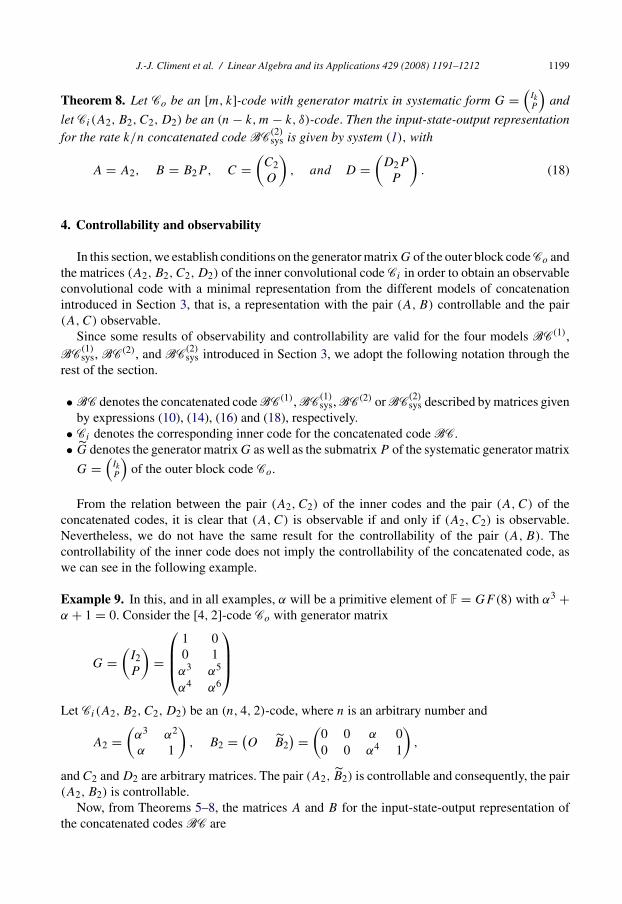
Theorem 8. Let Co be an [m, k]-code with generator matrix in systematic form G =(

IkP

)and

let Ci (A2, B2, C2, D2) be an (n − k, m − k, δ)-code. Then the input-state-output representationfor the rate k/n concatenated code BC

(2)sys is given by system (1), with

A = A2, B = B2P, C =(

C2O

), and D =

(D2P

P

). (18)

4. Controllability and observability

In this section, we establish conditions on the generator matrix G of the outer block codeCo andthe matrices (A2, B2, C2, D2) of the inner convolutional code Ci in order to obtain an observableconvolutional code with a minimal representation from the different models of concatenationintroduced in Section 3, that is, a representation with the pair (A, B) controllable and the pair(A, C) observable.

Since some results of observability and controllability are valid for the four models BC(1),BC

(1)sys, BC(2), and BC

(2)sys introduced in Section 3, we adopt the following notation through the

rest of the section.

• BC denotes the concatenated codeBC(1),BC(1)sys,BC(2) orBC

(2)sys described by matrices given

by expressions (10), (14), (16) and (18), respectively.• Ci denotes the corresponding inner code for the concatenated code BC.• G denotes the generator matrix G as well as the submatrix P of the systematic generator matrix

G =(

IkP

)of the outer block code Co.

From the relation between the pair (A2, C2) of the inner codes and the pair (A, C) of theconcatenated codes, it is clear that (A, C) is observable if and only if (A2, C2) is observable.Nevertheless, we do not have the same result for the controllability of the pair (A, B). Thecontrollability of the inner code does not imply the controllability of the concatenated code, aswe can see in the following example.

Example 9. In this, and in all examples, α will be a primitive element of F = GF(8) with α3 +α + 1 = 0. Consider the [4, 2]-code Co with generator matrix

G =(

I2P

)=

⎛⎜⎜⎝1 00 1α3 α5

α4 α6

⎞⎟⎟⎠Let Ci (A2, B2, C2, D2) be an (n, 4, 2)-code, where n is an arbitrary number and

A2 =(

α3 α2

α 1

), B2 = (

O B2) =

(0 0 α 00 0 α4 1

),

and C2 and D2 are arbitrary matrices. The pair (A2, B2) is controllable and consequently, the pair(A2, B2) is controllable.

Now, from Theorems 5–8, the matrices A and B for the input-state-output representation ofthe concatenated codes BC are

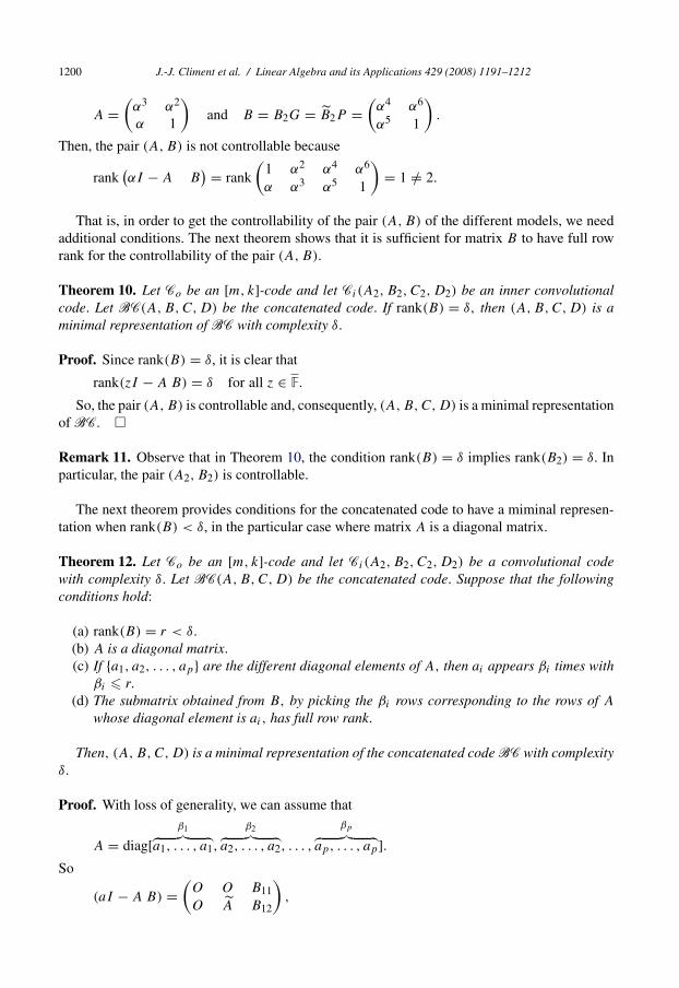
1200 J.-J. Climent et al. / Linear Algebra and its Applications 429 (2008) 1191–1212

A =(

α3 α2

α 1

)and B = B2G = B2P =

(α4 α6

α5 1

).

Then, the pair (A, B) is not controllable because

rank(αI − A B

) = rank

(1 α2 α4 α6

α α3 α5 1

)= 1 /= 2.

That is, in order to get the controllability of the pair (A, B) of the different models, we needadditional conditions. The next theorem shows that it is sufficient for matrix B to have full rowrank for the controllability of the pair (A, B).

Theorem 10. Let Co be an [m, k]-code and let Ci (A2, B2, C2, D2) be an inner convolutionalcode. Let BC(A, B, C, D) be the concatenated code. If rank(B) = δ, then (A, B, C, D) is aminimal representation of BC with complexity δ.

Proof. Since rank(B) = δ, it is clear that

rank(zI − A B) = δ for all z ∈ F.

So, the pair (A, B) is controllable and, consequently, (A, B, C, D) is a minimal representationof BC. �

Remark 11. Observe that in Theorem 10, the condition rank(B) = δ implies rank(B2) = δ. Inparticular, the pair (A2, B2) is controllable.

The next theorem provides conditions for the concatenated code to have a miminal represen-tation when rank(B) < δ, in the particular case where matrix A is a diagonal matrix.

Theorem 12. Let Co be an [m, k]-code and let Ci (A2, B2, C2, D2) be a convolutional codewith complexity δ. Let BC(A, B, C, D) be the concatenated code. Suppose that the followingconditions hold:

(a) rank(B) = r < δ.

(b) A is a diagonal matrix.(c) If {a1, a2, . . . , ap} are the different diagonal elements of A, then ai appears βi times with

βi � r.

(d) The submatrix obtained from B, by picking the βi rows corresponding to the rows of A

whose diagonal element is ai, has full row rank.

Then, (A, B, C, D) is a minimal representation of the concatenated code BC with complexityδ.

Proof. With loss of generality, we can assume that

A = diag[β1︷ ︸︸ ︷

a1, . . . , a1,

β2︷ ︸︸ ︷a2, . . . , a2, . . . ,

βp︷ ︸︸ ︷ap, . . . , ap].

So

(aI − A B) =(

O O B11

O A B12

),

J.-J. Climent et al. / Linear Algebra and its Applications 429 (2008) 1191–1212 1201

where

A = diag[β2︷ ︸︸ ︷

a1 − a2, . . . , a1 − a2, . . . ,

βp︷ ︸︸ ︷a1 − ap, . . . , a1 − ap].

Then, from condition (d), rank(B11) = β1 and, consequently,

rank(a1I − A B ) = δ.

The same argument follows for the rest of the elements in the diagonal of A. Therefore (A, B)

is controllable. �

As an immediate consequence of this theorem, we have the following corollaries.

Corollary 13. With the same notation as in Theorem 12, if the following conditions hold:

(a) rank(B) < δ.

(b) A is a diagonal matrix.(c) β1 = · · · = βp = 1.

(d) Each row of B has at least a nonzero element.

Then (A, B, C, D) is a minimal representation of the concatenated code BC with complexityδ.

Corollary 14. With the same notation as in Theorem 12, if the following conditions hold:

(a) k = 1.

(b) δ > 1.

(c) A is a diagonal matrix.(d) β1 = · · · = βp = 1.

(e) All elements of B are nonzero.

Then (A, B, C, D) is a minimal representation of the concatenated code BC with complexityδ.

5. Column distances and free distances

Once we get conditions that ensure us to have an observable concatenated convolutional codewith minimal representation, the aim of this section is to obtain strongly MDS convolutionalcodes from the concatenation of MDS codes or non MDS codes. For this purpose, we study someproperties of the column distances and the free distances of the concatenated codes. In the rest ofthe paper, we assume that the concatenated code is an observable convolutional code.

First of all, we provide a lower bound on the column distances of the concatenated codesBC(1)

and BC(1)sys, in terms of the column distances of the inner code Ci .

Theorem 15. LetCo be an [m, k]-code with generator matrix G. LetCi be an (n + m − k, m, δ)-code with maximum distance profile. If n � k + m − 2, then

1202 J.-J. Climent et al. / Linear Algebra and its Applications 429 (2008) 1191–1212

dcj (BC(1)) � dc

j (Ci ) − m(j + 1) + 1 f or j = 0, 1, . . . , L, (19)

where L = ⌊δm

⌋ +⌊

δn−k

⌋.

Proof. Suppose that (y0, y1, . . . , yj ; u0, u1, . . . , uj )T is a codeword of BC(1) with u0 /= 0; then

wt(Gu0, Gu1, . . . , Guj ) = r � dmin(Co). (20)

Now, from Theorem 4, every minor of matrix TL which is non trivially zero, is nonzero, andthen at most r − 1 rows of TL are orthogonal to (Gu0, Gu1, . . . , Guj )

T, because Guo /= 0. Sofrom expression (4), we obtain that at most r − 1 components of (y0, y1, . . . , yj )

T are zero, andconsequently,

wt(y0, y1, . . . , yj

)� (n − k)(j + 1) − (r − 1).

Now, taking into account that

wt(u0, u1, . . . , uj

)� 1, wt

(Gu0, Gu1, . . . , Guj

)� m(j + 1)

and expression (20), we have

wt(y0, y1, . . . , yj , u0, u1, . . . , uj ) = wt(y0, y1, . . . , yj ) + wt(u0, u1, . . . , uj )

� (n − k)(j + 1) − (r − 1) + 1

� (n − k)(j + 1) − m(j + 1) + 2

= dcj (Ci ) − m(j + 1) + 1 (21)

for j = 0, 1, . . . , L. Then, expression (19) follows from expressions (3) and (21). �

The next theorem, whose proof is similar to the previous one, gives a lower bound on thecolumn distances of the concatenated code BC

(1)sys.

Theorem 16. Let Co be an [m, k]-code with generator matrix in systematic form G =(

IkP

).

Suppose that the matrix P has rank k. Let Ci be an (n + m − 2k, m − k, δ)-code with maximumdistance profile, then

dcj (BC(1)

sys) � (n − m)(j + 1) + 2 f or j = 0, 1, . . . , L,

where

L =⌊

δ

m − k

⌋+

⌊δ

n − k

⌋. (22)

Observe that if in the previous theorem Co is an MDS block code, then through Theorem 1,we can ensure that rank(P ) = k, and consequently, we have the following result.

Corollary 17. Let Co be an [m, k]-MDS code with a generator matrix G =(

IkP

). Suppose that

k � m − k and let Ci be an (n + m − 2k, m − k, δ)-code with maximum distance profile, then

dcj (BC(1)

sys) � (n − m)(j + 1) + 2 f or j = 0, 1, . . . , L

where L is given by expression (22).

J.-J. Climent et al. / Linear Algebra and its Applications 429 (2008) 1191–1212 1203

Next, we obtain, for the concatenated codes BC(2) and BC(2)sys a lower bound on the column

distances in terms of the minimum distance of the outer block code and the column distances ofthe inner convolutional code. This result allows us to obtain a lower bound for the free distances.

Lemma 18. Let BC(2) be the concatenated code given by Theorem 7 from the outer block codeCo and the inner convolutional code Ci . Then,

dcj (BC(2)) � max{dmin(Co) + 1, dc

j (Ci ) + 1} f or j = 0, 1, 2, . . . (23)

Proof. Taking into account the relations between yt , y(2)t ; ut , u

(1)t , u

(2)t , and vt , v

(1)t , v

(2)t given

by expressions (5)–(7) and (15) (see also the comments before Theorem 7), we have

j∑t=0

wt(ut ) +j∑

t=0

wt(yt ) =j∑

t=0

wt(u

(1)t

)+

j∑t=0

wt(y

(2)t

)+

j∑t=0

wt(Gu

(1)t

)� wt

(u

(1)0

)+ wt

(Gu

(1)0

). (24)

So, from the definition of dmin(Co), expression (3), and the fact that u0 = u(1)0 , we obtain

dcj (BC(2)) � min

u(1)0 /=0

{wt

(u

(1)0

)+ wt

(Gu

(1)0

)}� 1 + dmin(Co). (25)

Similarly, from expressions (5), (6), (7) and (15) (see also the comments before Theorem 7) weobtain

j∑t=0

wt(ut ) +j∑

t=0

wt(yt ) =j∑

t=0

wt(u

(1)t

)+

j∑t=0

wt(y

(2)t

)+

j∑t=0

wt(u

(2)t

)

� wt(u

(1)0

)+

j∑t=0

wt(y

(2)t

)+

j∑t=0

wt(u

(2)t

).

Now, since u(2)0 = Gu

(1)0 and rank(G) = k, we have u0 = u

(1)0 /= 0 if and only if u

(2)0 = Gu

(1)0 /=

0. Therefore, from the above inequality and expression (3), we have

dcj (BC(2)) = min

u0 /=0

⎧⎨⎩j∑

t=0

wt(ut ) +j∑

t=0

wt(yt )

⎫⎬⎭� min

u(1)0 /=0

⎧⎨⎩wt(u

(1)0

)+

j∑t=0

wt(y

(2)t

)+

j∑t=0

wt(u

(2)t

)⎫⎬⎭� 1 + dc

j (Ci ). (26)

So inequality (23) follows from inequalities (25) and (26). �

Now, as an immediate consequence of expression (2) and the above lemma, we obtain thefollowing result.

1204 J.-J. Climent et al. / Linear Algebra and its Applications 429 (2008) 1191–1212

Theorem 19. Let BC(2) be the concatenated code given by Theorem 7 from the outer block codeCo and the inner convolutional code Ci . Then

dfree(BC(2)) � max{dmin(Co) + 1, dfree(Ci ) + 1}.

The free distance of the concatenated code BC(2)sys is always lower bounded by the minimum

distance of the outer block code, as in the case of the code BC(2) (see Lemma 21(a) below).Nevertheless, we cannot ensure that the free distance of the inner convolutional code is also alower bound of dfree(BC

(2)sys), as we can see in the following example.

Example 20. Let Co be the [5, 2]-code with systematic generator matrix

G =(

I2P

)=

⎛⎜⎜⎜⎜⎝1 00 11 α

α α2

0 0

⎞⎟⎟⎟⎟⎠ .

Observe that the nonsystematic part P of G has rank(P ) = 1 < 2, so Co is not an MDS blockcode. In fact, dmin(Co) = 2 < 4, which is the Singleton bound. Let Ci (A2, B2, C2, D2) be the(6, 3, 1)-code described by matrices

A2 = (α), B2 = (α 0 1), C2 =⎛⎝ 1

α2

α3

⎞⎠ , and D2 =⎛⎝ 1 α α2

α2 1 α3

α α4 α6

⎞⎠ ,

which is a maximum distance profile code with dfree(Ci ) = 4.So, through Theorems 8 and 10, the matrices

A = (α), B = (α α2), C2 =

⎛⎜⎜⎜⎜⎜⎜⎝

1α2

α3

000

⎞⎟⎟⎟⎟⎟⎟⎠ , and D2 =

⎛⎜⎜⎜⎜⎜⎜⎝

α6 1α4 α5

α6 11 α

α α2

0 0

⎞⎟⎟⎟⎟⎟⎟⎠are a minimal representation of the observable code BC

(2)sys with

dfree(BC(2)sys) = 2 < 4 = dfree(Ci ).

As we show in the next result, the fact that the matrix P has full column rank ensures thatdfree(Ci ) is a lower bound of dfree(BC

(2)sys).

Lemma 21. Let BC(2)sys be the concatenated code given by Theorem 8 from the outer block code

Co and the inner convolutional code Ci . Then

(a) dcj (BC

(2)sys) � dmin(Co) for j = 0, 1, 2, . . .

(b) If rank(P ) = k, then dcj (BC

(2)sys) � dc

j (Ci ) + 1 for j = 0, 1, 2, . . .

J.-J. Climent et al. / Linear Algebra and its Applications 429 (2008) 1191–1212 1205

Proof. Taking into account the relations between yt , y(1)t , y

(2)t ; ut , u

(1)t , u

(2)t , and vt , v

(1)t , v

(2)t

given by expressions (11), (12), (13) and (17) (see also the comments before Theorem 8) and witha similar argument to the one used to obtain inequality (24) in the proof of Lemma 18, we obtain

j∑t=0

wt(ut ) +j∑

t=0

wt(yt ) � wt(u

(1)0

)+ wt

(Pu

(1)0

)= wt

(Gu

(1)0

).

So, through expression (3) and taking into account that u0 = u(1)0 , we obtain the inequality of part

(a).Similarly, from expressions (11), (12), (13) and (17) we obtain

j∑t=0

wt(ut ) +j∑

t=0

wt(yt ) =j∑

t=0

wt(u

(1)t

)+

j∑t=0

wt(y

(2)t

)+

j∑t=0

wt(u

(2)t

)

� wt(u

(1)0

)+

j∑t=0

wt(y

(2)t

)+

j∑t=0

wt(u

(2)t

).

Now, since u(2)t = Pu

(1)t and rank(P ) = k, we have that u0 = u

(1)0 /= 0 if and only if u

(2)0 =

Pu(1)0 /= 0. Therefore, from the above inequality and expression (3) we have that

dcj (BC(2)

sys) � minu

(1)0 /=0

⎧⎨⎩wt(u

(1)0

)+

j∑t=0

wt(y

(2)t

)+

j∑t=0

wt(u

(2)t

)⎫⎬⎭ � 1 + dcj (Ci )

because u0 = u(1)0 . �

As an immediate consequence of expression (2) and the above lemma, we obtain the followingresult.

Theorem 22. Let BC(2)sys be the concatenated code given by Theorem 8 from the outer block code

Co and the inner convolutional code Ci . Then

(a) dfree(BC(2)sys) � dmin(Co).

(b) If rank(P ) = k, then dfree(BC(2)sys) � dfree(Ci ) + 1.

Our question now is how to obtain an optimal convolutional code from the concatenationof a block code and a convolutional code. One could think that if the constituent codes of theconcatenation are the best possible codes, that is, the outer code and the inner code are MDS blockcode and strongly MDS convolutional code, respectively, then the concatenated code would be a“good” code. In general, it is not true for the concatenated code BC(1), as shown in the followingexample.

Example 23. Consider the MDS [3, 2]-code Co with generator matrix

G =⎛⎝α3 α6

α α2

1 1

⎞⎠ .

Now, let Ci (A2, B2, C2, D2) be the (4, 3, 1)-code, where

1206 J.-J. Climent et al. / Linear Algebra and its Applications 429 (2008) 1191–1212

A2 = (1), B2 = (1 α α2), C2 = (1), and D2 = (1 1 1).

Observe that the pair (A2, C2) is observable. Furthermore, from Theorem 4, Ci is a strongly MDSconvolutional code with dfree(Ci ) = dc

1(Ci ) = 3.So, by applying Theorems 5 and 10, the minimal representation of the observable (3, 2, 1)-code

BC(1) is given by matrices

A = (1), B = (α3 α), C = (1), and D = (0 0).

But BC(1) is not an MDS convolutional code since dfree(BC(1)) = 2 < 3, which is the Sin-gleton bound.

As a consequence of the above example, the fact that the outer and the inner codes are optimalcodes, does not guarantee that the concatenated code BC(1) has large free distance. Furthermore,it is possible for the constituent codes to have a bad minimum and free distances, however, theconcatenated code BC(1) has maximum possible free distance, as we can see in the followingexample.

Example 24. Let Co be the [2, 1]-code with generator matrix

G =(

α

0

).

Since dmin(Co) = 1 < 2, this code is not an MDS block code.Now, let Ci (A2, B2, C2, D2) be the (3, 2, 1)-code, where

A2 = (α), B2 = (1 0), C2 = (1), and D2 = (1 0).

Then, the pair (A2, C2) is observable. Furthermore, we obtain that dfree(Ci ) = 1 < 3, which isthe Singleton bound. So Ci is not an MDS convolutional code.

Through Theorems 5 and 10, the minimal representation of the observable (2,1,1)-code BC(1)

is given by matrices

A = (α), B = (α), C = (1), and D = (α).

In addition, dc2(BC(1)) = 4, which is the Singleton bound, so the concatenated code BC(1) is a

strongly MDS convolutional code.

From the above examples, we conclude that the concatenated code BC(1) does not inherit thefree distance properties of the constituent codes. The next theorem provides a sufficient conditionfor the concatenated code BC(1) to be a strongly MDS convolutional code.

Theorem 25. Let BC(1) be the concatenated code described by expression (10) from the [m, k]-code Co and the (m + 1, m, 1)-code Ci , with k > 1. If the matrix

(D2G

C2B2G

)is the nonsystematic

part of a generator matrix of an MDS [k + 2, k]-code, then the concatenated code BC(1) is amaximum distance profile (k + 1, k, 1)-code.

Proof. Taking into account that⎛⎝ Ik

D2G

C2B2G

⎞⎠

J.-J. Climent et al. / Linear Algebra and its Applications 429 (2008) 1191–1212 1207

is the systematic generator matrix of an MDS [k + 1, k]-code, from Theorem 1 every minor of(D2G O

C2B2G D2G

)which is non trivially zero is nonzero. So by applying Theorem 4, BC(1) is a maximum distanceprofile convolutional code. �

Next, taking into account Remark 3, we obtain the following consequence of Theorem 25.

Corollary 26. LetBC(1) be the concatenated code described by expression (10), from the [m, k]-code Co and the (m + 1, m, 1)-code Ci . If the matrix

(D2G

C2B2G

)is the nonsystematic part of a

generator matrix of an MDS [k + 2, k]-code, then the concatenated code BC(1) is a stronglyMDS (k + 1, k, 1)-code.

For the concatenated code BC(1)sys, we have similar results. BC

(1)sys can be a non MDS convo-

lutional code even if the outer code is an MDS block code and the inner code is a strongly MDSconvolutional code, as we show in the following example.

Example 27. Consider the MDS [4, 1]-code Co with systematic generator matrix

G =

⎛⎜⎜⎝1α

1α3

⎞⎟⎟⎠ =(

I1P

).

Now, let Ci (A2, B2, C2, D2) be the strongly MDS (4, 3, 1)-code as in Example 23.So, by applying Theorems 6 and 10, the minimal representation of the observable (2,1,1)-code

BC(1)sys is given by matrices

A = (1), B = (α5), C = (1), and D = (0).

But dfree(BC(1)sys) = 3 < 4, which is the Singleton bound. So the concatenated code BC

(1)sys is not

an MDS convolutional code.

Furthermore, the concatenated code BC(1)sys can be a strongly MDS convolutional code even if

the constituent codes have bad minimum and free distances, as we show in the following example.

Example 28. Let Co be the [3, 1]-code with systematic generator matrix

G =⎛⎝1

α

0

⎞⎠ =(

I1P

).

We obtain that dmin(Co) = 2 < 3, which is the Singleton bound. So Co is not an MDS blockcode.

Now, let Ci (A2, B2, C2, D2) be the (3, 2, 1)-code, where

A2 = (α), B2 = (1 0), C2 = (α6), and D2 = (1 0).

Observe that the pair (A2, C2) is observable. Furthermore, we obtain that dfree(Ci ) = 1 < 3,which is the Singleton bound. So Ci is not an MDS convolutional code.

1208 J.-J. Climent et al. / Linear Algebra and its Applications 429 (2008) 1191–1212

Through Theorems 6 and 10, the minimal representation of the observable (2,1,1)-code BC(1)sys

is given by matrices

A = (α), B = (α), C = (α6), and D = (α).

We obtain that dc2(BC

(1)sys) = 4, which is the Singleton bound, so the concatenated code BC

(1)sys is

a strongly MDS convolutional code.

From the above examples, we conclude, as for the concatenated code BC(1), that the codeBC

(1)sys does not inherit the MDS property of the constituent codes. The next theorem, whose

proof is similar to that of Theorem 25, provides sufficient condition to obtain a strongly MDSconvolutional code BC

(1)sys.

Theorem 29. Let BC(1)sys be the concatenated code described by expression (14), from the [m, k]-

code Co and the (m − k + 1, m − k, 1)-code Ci , with k > 1. If the matrix(

D2P

C2B2P

)is the non-

systematic part of the generator matrix of an MDS [k + 2, k]-code, then the concatenated codeBC

(1)sys is a maximum distance profile (k + 1, k, 1)-code.

Similarly to Corollary 26 and taking into account Remark 3, we obtain the following conse-quence of Theorem 29.

Corollary 30. LetBC(1)sys be the concatenated code described by expression (14), from the [m, k]-

code and the (m − k + 1, m − k, 1)-code. If the matrix(

D2P

C2B2P

)is the nonsystematic part of a

generator matrix of an MDS [k + 2, k]-code, then the concatenated code BC(1)sys is a strongly

MDS (k + 1, k, 1)-code.

If the outer block code has dimension 1, we get the following two results for the concatenatedcode BC(1), which are similar to Theorem 25 and Corollary 26 respectively.

Theorem 31. Let BC(1) be the concatenated code described by expression (10), from the [m, 1]-code Co and the (m + 1, m, 1)-code Ci . If the vectors

DT2 , (C2B2)

T, (C2A2B2)T and (C2B2GC2B2 − C2A2B2GD2)

T

are not in C⊥o , then the concatenated code BC(1) is a maximum distance profile (2, 1, 1)-code.

Proof. The conditions of the theorem and the definition of the dual code of Co, allow us to ensurethat the matrix

T2 =⎛⎝ D2G

C2B2G D2G

C2A2B2G C2B2G D2G

⎞⎠ =⎛⎝ D

CB D

CAB CB D

⎞⎠has the property that every minor which is non trivially zero is nonzero (observe that in this caseL = � 1

1� + � 11� = 2). So, through Theorem 4, BC(1) has a maximum distance profile. �

Corollary 32. LetCo be an [m, 1]-code and letCi be an (m + 1, m, 1)-code.LetBC(1)(A, B, C, D)

be the concatenated code described by expression (10). If the vectors

J.-J. Climent et al. / Linear Algebra and its Applications 429 (2008) 1191–1212 1209

DT2 , (C2B2)

T, (C2A2B2)T and (C2B2GC2B2 − C2A2B2GD2)

T

are not in C⊥o , then the concatenated code BC(1) is a strongly MDS (2, 1, 1)-code.

Furthermore, if the outer block code has dimension one, we get two similar results for theconcatenated code BC

(1)sys. Since the proofs are analogous, they are omitted.

Theorem 33. Let BC(1)sys be the concatenated code described by expression (14), from the [m, 1]-

code Co and the (m, m − 1, 1)-code Ci . If the vectors(O

DT2

),

(O

(C2B2)T

),

(O

(C2A2B2)T

), and

(O

(C2B2GC2B2 − C2A2B2GD2)T

)are not in C⊥

o , then the concatenated code BC(1)sys is a maximum distance profile (2, 1, 1)-code.

Corollary 34. LetBC(1)sys be the concatenated code described by expression (14), from the [m, 1]-

code Co and the (m, m − 1, 1)-code Ci . If the vectors(O

DT2

),

(O

(C2B2)T

),

(O

(C2A2B2)T

)and

(O

(C2B2GC2B2 − C2A2B2GD2)T

)are not in C⊥

o , then the concatenated code BC(1)sys is a strongly MDS (2, 1, 1)-code.

Finally, for the concatenated codes BC(2) and BC(2)sys we cannot obtain conditions in order to

have a maximum distance profile concatenated code. In fact, as shown in the following theorem,these codes cannot have a maximum distance profile. The proof is a consequence of Theorem 4

and the fact that the matrix C of BC(2) and BC(2)sys is C =

(C2O

).

Theorem 35. Let BC(2) and BC(2)sys be the concatenated codes described by expression (16) and

(18), respectively, from the outer block code Co and the inner convolutional code Ci . Assumethat the pair (A, C) is observable, then, BC(2) and BC

(2)sys cannot have a maximum distance

profile.

Remark 36. As a consequence of Theorem 35 and Remark 3, if n − k divides δ, the codes BC(2)

and BC(2)sys cannot have the strongly MDS property.

6. The relations between different models of concatenation

In this section, we analyse the relations between different models of concatenation, in order todetermine which models give the best results. Although, we have analysed many examples (see[12]), including those from the F = GF(4) field , only the most important are presented here, allof them from the F = GF(8) field. In fact, it is only possible to compare the first model to thethird model (see Fig. 1 and 3) and the second model to the fourth model (see Fig. 2 and 4), sincethe same external and internal codes can be used for concatenation, although the concatenatedcodes obtained have different rates.

1210 J.-J. Climent et al. / Linear Algebra and its Applications 429 (2008) 1191–1212

Consider the [2, 1]-block code B1 with generator matrix P1 =(

0α6

)and the [3, 2]-block code

Bk generated by the matrix Pk , for k = 2, 3, 4, with

P2 =⎛⎝α3 1

1 α4

α6 α2

⎞⎠ , P3 =⎛⎝α2 α3

1 α

α6 0

⎞⎠ , P4 =⎛⎝α3 1

1 α2

α6 α4

⎞⎠ .

So, B4 is an MDS block code, whereas for k = 1, 2, 3, Bk is a non MDS block code.

Consider now the [3, 1]-block code Bs1, with systematic generator matrix G1 =

(I1P1

)and the

[5, 2]-block code Bsk , for k = 2, 3, 4 with systematic generator matrix Gk =

(I2Pk

). So, Bs

k is an

MDS block code, for k = 4, and it is a non MDS block code for k = 1, 2, 3.Let C1(A

(1)2 , B

(1)2 , C

(1)2 , D

(1)2 ) be the (3, 2, 1)-code generated by the matrices

A(1)2 = (α), B

(1)2 = (1 α), C

(1)2 = (1), D

(1)2 = (1 0),

and let C2(A(2)2 , B

(2)2 , C

(2)2 , D

(2)2 ) be the (4, 3, 1)-code generated by the matrices

A(2)2 = (1), B

(2)2 = (1 α α2), C

(2)2 = (1) and D

(2)2 = (1 1 1).

So, C1(A(1)2 , B

(1)2 , C

(1)2 , D

(1)2 ) is an MDS convolutional code, whereas C2(A

(2)2 , B

(2)2 , C

(2)2 , D

(2)2 )

is a strongly MDS convolutional code.In order to relate the different models of concatenation, we will denote both the block code

Bk (if we consider models 1 and 3) and the block code Bsk (if we consider models 2 and 4) by

Bk . Also, dSB will denote the Singleton bound for each concatenated code.In Table 1, we have considered the non MDS block codes B1 (for BC(1) and BC(2) concatena-

tions) andBs1 (forBC

(1)sys andBC

(2)sys concatenations) as the outer code and the MDS convolutional

codeC1 as the inner code. The result obtained is that no concatenated code is a convolutional MDScode, although the constituent codes are MDS. Furthermore, in this example, the free distance ofthe BC(1) and BC

(1)sys codes is closer to the corresponding Singleton bound than the free distance

of BC(2) and BC(2)sys codes.

However, if we consider the non MDS block codes B2 (for concatenations BC(1) and BC(2))and Bs

2 (for BC(1)sys and BC

(2)sys concatenations) as the outer code and the strongly MDS C2 convo-

lutional code as the inner code, the free distance of the BC(2) code is closer to the correspondingSingleton bound than the free distance of BC(1). We have the same result for the BC

(2)sys and

BC(1)sys codes, that is to say, the free distance of the BC

(2)sys code is closer to the Singleton bound

than the free distance of the BC(1)sys code (see Table 2).

Table 1Concatenation of B1 and C1 codes

Model ISO representation of BC dfree(BC) dfree(BC)/dSB

BC(1) A = (α), B = (1), C = (1), D = (0) dfree(BC) = 3 3/4

BC(1)sys Non MDS code

BC(2) A = (α), B = (1), C =⎛⎝1

00

⎞⎠, D =⎛⎝ 0

0α6

⎞⎠ dfree(BC) = 5 5/8

BC(2)sys Non MDS code

J.-J. Climent et al. / Linear Algebra and its Applications 429 (2008) 1191–1212 1211

Table 2Concatenation of B2 and C2 codes

Model ISO representation of BC dfree(BC) dfree(BC)/dSB

BC(1) A = (1), B = (α3 0), C = (1), D = (α5 α3) dfree(BC) = 2 2/3

BC(1)sys Non MDS code

BC(2) A = (1), B = (α3 0), C =

⎛⎜⎜⎝1000

⎞⎟⎟⎠, D =

⎛⎜⎜⎝α5 α3

α3 11 α4

α6 α2

⎞⎟⎟⎠ dfree(BC) = 5 5/6

BC(2)sys Non MDS code

Table 3 shows that it is possible for concatenated codes BC(1), BC(1)sys, BC(2) and BC

(2)sys to be

MDS.Furthermore, it is also possible for the BC(1) and BC

(1)sys codes to be MDS while the BC(2)

and BC(2)sys codes are not, as shown in Table 4.

Nevertheless, through the construction of different models of concatenation, it is assumed thatthe opposite is not possible, that is to say, if the concatenated codes BC(2) and BC

(2)sys are MDS

convolutional codes, then the concatenated codes BC(1) and BC(1)sys are necessarily MDS codes,

too.

Table 3Concatenation of B3 and C2 codes

Model ISO representation of BC dfree(BC)

BC(1) A = (1), B = (α2 α5), C = (1), D = (0 1) dfree(BC) = 3

BC(1)sys MDS code

BC(2) A = (1), B = (α2 α5), C =

⎛⎜⎜⎝1000

⎞⎟⎟⎠, D =

⎛⎜⎜⎝0 1α2 α3

1 α

α6 0

⎞⎟⎟⎠ dfree(BC) = 6

BC(2)sys MDS code

Table 4Concatenation of B4 and C2 codes

Model ISO representation of BC dfree(BC) dfree(BC)/dSB

BC(1) A = (1), B = (α3 α5), C = (1), D = (α3 α5) dc1(BC) = 3 3/3

BC(1)sys Strongly MDS code

BC(2) A = (1), B = (α3 α5), C =

⎛⎜⎜⎝1000

⎞⎟⎟⎠, D =

⎛⎜⎜⎝α3 α5

α3 11 α2

α6 α4

⎞⎟⎟⎠ dfree(BC) = 5 5/6

BC(2)sys Non MDS code

1212 J.-J. Climent et al. / Linear Algebra and its Applications 429 (2008) 1191–1212

References

[1] S. Benedetto, D. Divsalar, G. Montorsi, F. Pollara, Serial concatenation of interleaved codes: Performance analysis,design and iterative decoding, IEEE Trans. Inform. Theory 44 (3) (1998) 909–926.

[2] S. Benedetto, G. Montorsi, Serial concatenation of block and convolutional codes, Electron. Lett. 32 (13) (1996)887–888.

[3] S. Benedetto, G. Montorsi, Unveiling turbo codes: Some results on parallel concatenated coding schemes, IEEETrans. Inform. Theory 42 (1996) 409–428.

[4] C. Berrou, A. Glavieux, P. Thitimajshima, Near Shannon limit error-correcting coding and decoding: turbo codes(1), International Conference on Communication, IEEE, Geneva, Switzerland, 1993, pp. 1064–1070.

[5] C. Berrou, M. Jézéquel, Non binary convolutional codes for turbo coding, Electron. Lett. 35 (1) (1999) 39–40.[6] J.-J. Climent, V. Herranz, C. Perea, Composite linear time invariant systems and its applications to convolutional

codes, The Fifth International Conference on Engineering Computational Technology, Civil-Comp Press, 2006, pp.203–204.

[7] J.-J. Climent, V. Herranz, C. Perea, A first approximation of concatenated convolutional codes from linear systemstheory viewpoint, Linear Algebra Appl. 425 (2007) 673–699.

[8] G.D. Forney Jr., Concatenated Codes, M.I.T. Press, Cambridge, MA, 1966.[9] J. Freudenberger, M. Bossert, S. Shavgulidze, V. Zyablov, Woven codes with outer warp: Variations, design, and

distance properties, IEEE J. Select. Areas Commun. 19 (5) (2001) 813–824.[10] J. Hagenauer, P. Hoeher, Concatenated viterbi decoding, in: Proceedings of the Fourth Joint Swedish-Soviet Inter-

national Workshop on Information Theory, Gotland, Sweden, 1989, pp. 29–33.[11] M. Hautus, Controllability and observability condition for linear autonomous systems, Proceedings of Nedderlandse

Akademie voor Wetenschappen, Series A 72 (1969) 443–448.[12] V. Herranz, Estudio y construcción de códigos convolucionales: códigos perforados, códigos concatenados desde el

punto de vista de sistemas (Spanish). PhD Thesis, Universidad Miguel Hernández de Elche, Spain. March 2007.[13] S. Höst, R. Johannesson, V. Sidorenko, K.S. Zigangirov, V. Zyablov, A first encounter with binary woven convo-

lutional codes, in: Proceedings of the 4th International Symposium on Communication Theory and Applications,Lake Districts, UK, 1997, 13–18.

[14] S. Höst, R. Johannesson, V. Sidorenko, K.S. Zigangirov, V. Zyablov, Woven convolutional codes i: Encoder prop-erties, IEEE Trans. Inform. Theory 48 (4) (2002) 149–161.

[15] R. Hutchinson, J. Rosenthal, R. Smarandache, Convolutional codes with maximum distance profile,Systems ControlLett. 54 (1) (2005) 53–63.

[16] R. Jordan, S. Höst, R. Johannesson, M. Bosset, V.V. Zyablov, Woven convolutional codes ii: Decoding aspects, IEEETrans. Inform. Theory 50 (10) (2004) 2522–2529.

[17] L.C. Perez, J. Seghers, D.J. Costello, A Distance Spectrum Interpretation of Turbo Codes, IEEE Trans. Inform.Theory 42 (1996) 1698–1709.

[18] S. Roman, Coding and Information Theory, Springer-Verlag, New York, 1992.[19] J. Rosenthal, J. Schumacher, E.V. York, On behaviors and convolutional codes, IEEE Trans. Inform. Theory 42 (6)

(1996) 1881–1891.[20] J. Rosenthal, R. Smarandache, Maximum distance separable convolutional codes, Applicable algebra in engineering,

Commun. Comput. 10 (1999) 15–32.[21] J. Rosenthal, E.V. York, BCH convolutional codes, IEEE Trans. Inform. Theory 45 (6) (1999) 1833–1844.[22] C.E. Shannon, A mathematical theory of communication, The Bell System Tech. J. 27 (1948) 379–423., 623–656.