1

Convolutional Codes in Rank Metric withApplication to Random Network Coding

Antonia Wachter-Zeh, Markus Stinner, Vladimir Sidorenko

Abstract—Random network coding recently attracts attentionas a technique to disseminate information in a network. Thispaper considers a non-coherent multi-shot network, where theunknown and time-variant network is used several times. In orderto create dependencies between the different shots, particularconvolutional codes in rank metric are used. These codes areso-called (partial) unit memory ((P)UM) codes, i.e., convolutionalcodes with memory one. First, distance measures for convolu-tional codes in rank metric are shown and two constructions of(P)UM codes in rank metric based on the generator matrices ofmaximum rank distance codes are presented. Second, an efficienterror-erasure decoding algorithm for these codes is presented.Its guaranteed decoding radius is derived and its complexity isbounded. Finally, it is shown how to apply these codes for errorcorrection in random linear and affine network coding.

Index Terms—convolutional codes, network coding, (partial)unit memory codes, rank-metric codes

I. INTRODUCTION

Random linear network coding (RLNC, see e.g., [2]–[4])and more recently, random affine network coding (RANC,see [5]), are powerful means for distributing information innetworks. In these models, it is assumed that the packetsare vectors over a finite field and that each internal nodeof the network performs a random linear (or random affine,respectively) combination of all packets received so far andforwards this random combination to adjacent nodes. Noticethat affine combinations are particular linear combinations, see[5].

When we consider the transmitted packets as rows of amatrix, then the linear combinations performed by the nodesare elementary row operations on this matrix. During anerror- and erasure-free transmission over such a network, therow space of the transmitted matrix is therefore preserved.However, due to the linear combinations at the nodes, asingle erroneous packet can propagate widely throughout thenetwork. This makes error-correcting techniques in randomnetworks essential.

Parts of this work were presented at the IEEE International Symposiumon Network Coding 2012 (NETCOD), Cambridge, MA, USA, 2012 [1]. A.Wachter-Zeh’s work was supported in part by a Minerva Postdoctoral Fellow-ship and in part by the German Research Council “Deutsche Forschungs-gemeinschaft” (DFG) under Grant No. Bo867/21. M. Stinner’s work wassupported by an Alexander von Humboldt Professorship endowed by theGerman Federal Ministry of Education and Research. V. Sidorenko’s workwas supported by the German Research Council (DFG) under Grant No.Bo867/22.

A. Wachter-Zeh is with the Computer Science Department,Technion—Israel Institute of Technology, Haifa, Israel (e-mail:antonia@cs.technion.ac.il).

M. Stinner is with the Institute for Communications Engineering, TechnicalUniversity of Munich, Germany (e-mail: markus.stinner@tum.de).

V. Sidorenko is with the Institute for Communications Engineering, Tech-nical University of Munich, Germany (e-mail:vladimir.sidorenko@tum.de).

Based on these observations, Kotter and Kschischang [6]used subspace codes for error control in RLNC and introduceda channel model, called the operator channel. Silva, Kschis-chang and Kotter [7] showed that lifted rank-metric blockcodes result in almost optimal subspace codes for RLNC. Inparticular, they used Gabidulin codes [8]–[10], which are rank-metric analogs to Reed–Solomon codes. Both approaches wereextended to affine subspace codes by Gadouleau and Yan forerror correction in RANC [5].

In this paper, we consider non-coherent multi-shot networkcoding (see e.g., [11]). Therefore, we use the network severaltimes, where the internal structure of the network is unknownand might change in each shot. Creating dependencies betweenthe transmitted words of the different shots can help to copewith difficult error patterns and strongly varying channels. Weachieve these dependencies by using convolutional networkcodes.

In particular, we consider so-called (partial) unit memory((P)UM) codes [12], [13] in rank metric. (P)UM codes are aspecial class of convolutional codes with memory one. Theycan be constructed based on block codes, e.g., Reed–Solomon[14]–[16] or cyclic codes [17], [18]. The underlying blockcodes make an algebraic description of the convolutional codepossible, enable us to estimate the distance properties andallow us to take into account existing efficient block decodersin order to decode the convolutional code. Notice that aconvolutional code with arbitrary memory can be consideredas PUM convolutional code with larger block size. This isanother motivation to start working on (P)UM convolutionalcodes in rank metric; their generalization to multi-memorycodes in rank metric is an interesting topic for future work.

A convolutional code in Hamming metric can be charac-terized by its active row distance, which in turn is basicallydetermined by the free distance and the slope. These distancemeasures determine the error-correcting capability of the con-volutional code. In [12], [13], [15], [19], upper bounds on thefree (Hamming) distance and the slope of (P)UM codes werederived.

In [20], [21], distance measures for convolutional codes inrank metric were introduced and PUM codes based on theparity-check matrix of Gabidulin codes were constructed.

In this paper, we construct (P)UM codes based on the gen-erator matrix of Gabidulin codes and calculate their distanceproperties. As a distance measure, the sum rank metric isused, which is motivated by multi-shot network coding [11]and which is used to define the free rank distance and theactive row rank distance, see also [20], [21]. Moreover, weprovide an efficient decoding algorithm based on rank-metricblock decoders, which is able to handle errors and at the same

arX

iv:1

404.

7251

v2 [

cs.I

T]

19

Jan

2015

2

time column and row erasures. This decoding algorithm canbe seen as a generalization of the Dettmar–Sorger algorithm[22] to error-erasure decoding as well as to the rank metric.Further, we show how lifted PUM codes can be applied forerror-correction in RLNC and RANC.

There are other contributions devoted to convolutional net-work codes (see e.g. [23]–[26]). However, in most of thesepapers, convolutional codes are used to solve the problem ofefficiently mixing information in a multicast setup and none ofthese code constructions is based on codes in the rank metricand deals with the transmission over the operator channel asours. Our contribution can be seen as an equivalent to theblock code construction from [7].

This paper is structured as follows. In Section II, definitionsand notations for (lifted) rank-metric codes as well as forconvolutional codes are given. Section III shows distance mea-sures for convolutional codes in rank metric and in Section IV,we provide two explicit constructions of (P)UM codes basedon Gabidulin codes and we derive their distance properties.The first construction yields codes of low code rate, and isgeneralized by the second construction to arbitrary code rates.In Section V, we present an efficient decoding algorithm basedon rank-metric block decoders, which is able to handle errorsand row/column erasures. This decoding algorithm can be seenas a generalization of the Dettmar–Sorger algorithm [22]. InSection VI, we show—similar to [7]—how lifted (P)UM codescan be applied in RLNC and how decoding in RLNC reducesto error-erasure decoding of our (P)UM code construction,which can efficiently be decoded by our algorithm fromSection V. Finally, Section VII outlines how to apply our codesfor RANC and Section VIII concludes this paper.

II. PRELIMINARIES

A. Notations

Let q be a power of a prime and let us denote the q-powerfor any positive integer i by x[i] def

= xqi

. Let Fq denote thefinite field of order q and F = Fqm its extension field of orderqm. We use Fs×nq to denote the set of all s×n matrices over Fqand Fn = F1×n for the set of all row vectors of length n overF. LetRq (A) denote the row space of a matrix A over Fq andlet Is denote the s × s identity matrix. Moreover, denote theelements of a vector a(i) ∈ Fn by a(i) = (a

(i)0 a

(i)1 . . . a

(i)n−1).

Throughout this contribution, let the rows and columns of anm×n-matrix A be indexed by 0, . . . ,m− 1 and 0, . . . , n− 1and denote the set of integers [a, b] = {i : a ≤ i ≤ b, i ∈ Z}.

Let β = (β0 β1 . . . βm−1) be an ordered basis of F overFq . There is a bijective map Φβ of any vector a ∈ Fn on amatrix A ∈ Fm×nq , denoted as follows:

Φβ : Fn → Fm×nq

a = (a0 a1 . . . an−1) 7→ A,

where A = Φβ (a) ∈ Fm×nq is defined such that aj =∑m−1i=0 Ai,jβi, ∀j ∈ [0, n − 1]. In the following, we use

both representations (as a matrix over Fq or as a vector overF), depending on what is more useful in the context.

Consider the vector space Fnq of dimension n over Fq .The Grassmannian of dimension r ≤ n is the set of all

subspaces of Fnq of dimension r and is denoted by Gq(n, r).The cardinality of Gq(n, r) is the so-called Gaussian binomial,calculated by ∣∣Gq(n, r)∣∣ =

[n

r

]def=

r−1∏i=0

qn − qiqr − qi ,

with the upper and lower bounds (see e.g. [6, Lemma 4])

qr(n−r) ≤[n

r

]≤ 4qr(n−r). (1)

For two subspaces U ,V in Fnq , we denote by U+V the smallestsubspace containing the union of U and V . The subspacedistance between U ,V in Fnq is defined by

dS(U ,V) = dim(U + V)− dim(U ∩ V)

= 2 dim(U + V)− dim(U)− dim(V).

It can be shown that the subspace distance is indeed a metric(see e.g. [6]).

B. Rank Metric and Gabidulin Codes

We define the rank norm rk(a) as the rank of A = Φβ (a) ∈Fm×nq over Fq . The rank distance between a and b is the rankof the difference of the two matrix representations (see [9]):

dR(a,b)def= rk(a− b) = rank(A−B).

The minimum rank distance d of a code C ⊆ Fn is definedby

ddef= min

a,b∈Ca6=b

{dR(a,b) = rk(a− b)

}.

For linear codes of length n ≤ m and dimension k, theSingleton-like upper bound [8]–[10] implies that d ≤ n−k+1.If d = n− k+ 1, the code is called a maximum rank distance(MRD) code.

Gabidulin codes are a special class of rank-metric codes andcan be defined in vector representation by its generator matrixas follows.

Definition 1 (Gabidulin Code [9]) A linear GA[n, k] codeC ⊆ Fn of length n ≤ m and dimension k is defined byits k × n generator matrix GG:

GG =

g0 g1 . . . gn−1

g[1]0 g

[1]1 . . . g

[1]n−1

......

. . ....

g[k−1]0 g

[k−1]1 . . . g

[k−1]n−1

,

where g0, g1, . . . , gn−1 ∈ F are linearly independent over Fq .

Gabidulin codes are MRD codes, i.e., d = n− k+ 1, see [9].Let the matrix C ∈ Fm×nq = Φβ (c), where c = u · GG

for some u ∈ Fk, be a transmitted codeword that is corruptedby an additive error matrix E ∈ Fm×nq . At the receiver side,only the received matrix R ∈ Fm×nq , where R = C + E, isknown. The channel might provide additional side informationin the form of erasures, which help to increase the decodingperformance. This additional side information of the channelis assumed to be given in form of:

3

• % row erasures (in [7] called “deviations”) and• γ column erasures (in [7] called “erasures”),

such that the received matrix can be decomposed into

R = C + A(R)B(R) + A(C)B(C) + A(E)B(E)︸ ︷︷ ︸=E

, (2)

where A(R) ∈ Fm×%q , B(R) ∈ F%×nq , A(C) ∈ Fm×γq , B(C) ∈Fγ×nq , A(E) ∈ Fm×tq , B(E) ∈ Ft×nq are full rank matrices.The channel outputs R and additionally A(R) and B(C) to thereceiver. Further, t denotes the number of errors without sideinformation. The decomposition from (2) is not necessarilyunique, but we can use any of them.

The rank-metric block bounded minimum distance (BMD)error-erasure decoding algorithms from [7], [27] can recon-struct any c ∈ GA[n, k] from r = Φ−1

β (R) with complexityO(n2) operations over F if

2t+ %+ γ ≤ d− 1 = n− k. (3)

C. Lifted Gabidulin Codes

A constant-dimension code is a subset of a certain Grass-mannian. We shortly recall the definition from [7] of a specialclass of constant-dimension codes, called lifted Gabidulincodes.

Let CDq(n,MS, dS, r) denote a constant-dimension code inGq(n, r) with cardinality MS and minimum subspace distancedS. The lifting of a block code is defined as follows.

Definition 2 (Lifting of Matrix or Code) Consider the map

lift : Fr×(n−r)q → Gq(n, r)

X 7→ Rq ([Ir X]) .

The subspace lift(X) = Rq ([Ir X]) is called lifting of thematrix X. If we apply this map on all codewords (in matrixrepresentation) of a code C, then the constant-dimension codelift(C) is called lifting of C.

The following lemma shows the properties of a liftedGabidulin code.

Lemma 1 (Lifted Gabidulin Code [7]) Let C be aGabidulin GA[r, k] code over Fqn−r of length r ≤ n − r,minimum rank distance d = r − k + 1 and cardinalityMR = q(n−r)k.

Then, the lifting of the transposed codewords, i.e.,

lift(CT )def={

lift(CT ) = Rq([Ir CT ]

): Φ−1

β (C) ∈ C}

is a CDq(n,MS, dS, r) constant-dimension code of cardinalityMS = MR = q(n−r)k, minimum subspace distance dS = 2dand lies in the Grassmannian Gq(n, r).

D. Convolutional Codes and (Partial) Unit Memory CodesIn practical realizations, it does not make sense to consider

(semi-)infinite sequences and therefore, we consider onlylinear zero-forced terminated convolutional codes. Such aconvolutional code C is defined by the following terminatednon-catastrophic Nk × (n(N + µ)) generator matrix G overF, for some integer N :

G =

G(0) G(1) . . . G(µ)

G(0) G(1) . . . G(µ)

. . . . . . . . . . . .G(0) G(1) . . . G(µ)

, (4)

where G(i), ∀i = 0, . . . , µ, are k × n-matrices and µ denotesthe memory of G, see [28] and Definition 3. Each codewordof C is a sequence of N + µ blocks of length n over F, i.e.,c = (c(0) c(1) . . . c(N+µ−1)), represented equivalently as asequence of m × n matrices over Fq , i.e., C = Φβ (c) =(C(0) C(1) . . . C(N+µ−1)).

Memory and constraint length are properties of the gener-ator matrix. We follow Forney’s notations [29] based on thepolynomial representation of the generator matrix:

G(D) = G(0) + G(1)D + G(2)D2 + · · ·+ G(µ)Dµ

=(gi,j(D)

)i∈[0,k−1]

j∈[0,n−1],

where gi,j(D) = g(0)i,j + g

(1)i,j D + · · ·+ g

(µ)i,j D

µ and g(l)i,j ∈ Fq ,

∀l ∈ [0, µ], ∀i ∈ [0, k − 1] and ∀j ∈ [0, n− 1].

Definition 3 (Constraint Length and Memory) The i-thconstraint length νi of a polynomial generator matrix G(D)is

νidef= max

j∈[0,n−1]

{deg gi,j(D)

}, ∀i ∈ [0, k − 1].

The memory of G(D) is

µdef= max

i∈[0,k−1]{νi},

and the overall constraint length of G(D) is ν def=∑k−1i=0 νi.

(P)UM codes are a special class of convolutional codes ofmemory µ = 1, introduced by Lee and Lauer [12], [13]. Thesemi-infinite generator matrix consists therefore of two k× nsubmatrices G(0) and G(1). These matrices both have full rankk if we want to construct a UM(n, k) unit memory code.

For a PUM(n, k, k(1)) partial unit memory code over F,rank(G(0)) = k and rank(G(1)) = k(1) < k has to hold.W.l.o.g., for PUM codes, we assume that the lowermost k −k(1) rows of G(1) are zero and we denote:

G(0) =

(G(00)

G(01)

), G(1) =

(G(10)

0

), (5)

where G(00) and G(10) are k(1)×n matrices of full rank andG(01) is a full-rank (k−k(1))×n matrix over F. The encodingrule for each code block of a (P)UM code is hence given by

c(i) = u(i) ·G(0) + u(i−1) ·G(1), ∀i = 1, 2, . . . , (6)

where u(i) and u(i−1) ∈ Fk for all i. The memory of (P)UMcodes is µ = 1. The overall constraint length is ν = k for UMcodes and ν = k(1) for PUM codes.

4

III. DISTANCE MEASURES FOR CONVOLUTIONAL CODESIN RANK METRIC

In this section, we provide distance measures and upperbounds for convolutional codes based on a special rank metric,see also [21]. This special rank metric—the sum rank metric—was proposed by Nobrega and Uchoa-Filho under the name“extended rank metric” in [11] for multi-shot transmissions ina network.

A. Distance Parameters and Trellis Description

In [11], it is shown that the sum rank distance and thesubspace distance of the modified lifting construction arerelated in the same way as the rank distance and the subspacedistance of the lifting construction, see [7] and also Lemma 1.Hence, the use of the sum rank metric for multi-shot networkcoding can be seen as the analog to using the rank metric forsingle-shot network coding.

The sum rank weight and distance are defined as follows.

Definition 4 (Sum Rank Weight/Distance) Let two vectorsa,b ∈ FnN be decomposed into N subvectors of length nsuch that:

a = (a(0) a(1) . . . a(N−1)), b = (b(0) b(1) . . . b(N−1)),

with a(i),b(i) ∈ Fn, ∀i ∈ [0, N − 1]. The sum rank weight ofa is the sum of the ranks of the subvectors:

wtΣ(a)def=

N−1∑i=0

rk(a(i)). (7)

The sum rank distance between a and b is the sum rank weightof the difference of the vectors:

dΣ(a,b)def= wtΣ(a− b) =

N−1∑i=0

rk(a(i) − b(i)). (8)

Since the rank distance is a metric (see e.g. [9]), the sum rankdistance is also a metric.

An important measure for convolutional codes in Hammingmetric is the free distance, and consequently, we define thefree rank distance in a similar way in the sum rank metric.

Definition 5 (Free Rank Distance) The free rank distance ofa convolutional code C is the minimum sum rank distance (8)between any two different codewords a,b ∈ C:

dfdef= min

a,b∈C,a6=b

{dΣ(a,b)

}= min

a,b∈C,a6=b

{N−1∑i=0

rk(a(i) − b(i))

}.

For a linear convolutional code, the free rank distance is df =mina∈C,a6=0

{wtΣ(a)

}. Throughout this paper, we consider

only linear convolutional codes.Any convolutional code can be described by a minimal

code trellis, which has a certain number of states and theinput/output blocks are associated to the edges of the trellis.The current state in the trellis of a (P)UM code over F canbe associated with the vector s(i) = u(i−1)G(1), see e.g.,[16], and therefore there are qmk

(1)

possible states. We call

the current state zero state if s(i) = 0. A code sequence ofa terminated (P)UM code with N blocks can therefore beconsidered as a path in the trellis, which starts in the zerostate and ends in the zero state after N edges.

The error-correcting capability of convolutional codes isdetermined by active distances, a fact that will become obviousin view of our decoding algorithm in Section V. In thefollowing, we define the active row/column/reverse columnrank distances analog to active distances in Hamming metric[19], [28], [30]. In the literature, there are different definitionsof active distances in Hamming metric. Informally stated, for aj-th order active distance of C, we simply look at all sequencesof length j, and require some conditions on the passed statesin the minimal code trellis of C.

Let C(r)j denote the set of all codewords in a convolutional

code C, corresponding to paths in the minimal code trelliswhich diverge from the zero state at depth zero and returnto the zero state for the first time after j branches at depthj. W.l.o.g., we assume that we start at depth zero, as weonly consider time-invariant convolutional codes. This set isillustrated in Figure 1.

States

Time

0 1 2 . . . j

C(r)j

Figure 1. The set C(r)j : it consists of all codewords of C having paths in theminimal code trellis which diverge from the zero state at depth 0 and returnto the zero state for the first time at depth j.

Definition 6 (Active Row Rank Distance) The active rowrank distance of order j of a linear convolutional code isdefined as

d(r)j

def= min

c∈C(r)j

{wtΣ(c)

}, ∀j ≥ 1.

Clearly, for non-catastrophic encoders [28], the minimum ofthe active row rank distances of different orders is the sameas the free rank distance, see Definition 5: df = minj

{d

(r)j

}.

The slope of the active row rank distance is defined as follows.

Definition 7 (Slope of Active Row Rank Distance) Theslope of the active row rank distance (Definition 6) is

σdef= lim

j→∞

{d

(r)j

j

}.

As in Hamming metric [31, Theorem 1], [32, Theorem 2.7],the active row rank distance of order j can be lower boundedby a linear function d

(r)j ≥ max{j · σ + β, df} for some

β ≤ df .Similar to Hamming metric, we can introduce an active

column rank distance and an active reverse column rankdistance. Let C(c)

j denote the set of all words in the trellis

5

of length j blocks, leaving the zero state at depth zero andending in any state at depth j and let C(rc)

j denote the set ofall words starting in any state at depth zero and ending in thezero state in depth j, both without zero states in between (seeFigures 2 and 3). The active column rank distance and theactive reverse column rank distance are then defined by:

d(c)j

def= min

c∈C(c)j

{wtΣ(c)

}, ∀j ≥ 1. (9)

d(rc)j

def= min

c∈C(rc)j

{wtΣ(c)

}, ∀j ≥ 1. (10)

States

0 1 2 . . . j

Figure 2. The set C(c)j : all codewords of C diverging from the zero state atdepth 0, where no zero states between depths 0 and j are allowed.

States

0 1 2 . . . j

Figure 3. The set C(rc)j : all codewords of C ending in the zero state at depthj, where no zero states between depths 0 and j are allowed.

B. Upper Bounds on Distances of (P)UM Codes

In the following, we recall upper bounds on the free rankdistance df (Definition 5) and the slope σ (Definition 7) forUM and PUM codes based on the sum rank metric (7), (8).The derivation of the bounds uses known bounds for (P)UMcodes in Hamming metric [12], [13], [15].

Corollary 1 (Upper Bounds [21, Corollary 1]) For aUM(n, k) code, where ν = k, the free rank distance isbounded by:

df ≤ 2n− k + 1. (11)

For a PUM(n, k, k(1)) code, where ν = k(1) < k, the freerank distance is bounded by:

df ≤ n− k + ν + 1. (12)

For both, UM and PUM codes, the slope is bounded by:

σ ≤ n− k. (13)

IV. CONSTRUCTION OF CONVOLUTIONAL CODES IN RANKMETRIC

This section provides a construction of (P)UM codes whosesubmatrices of the generator matrix define Gabidulin codes.In the first step (Section IV-A), we adapt the constructionfrom [22] in Hamming metric to rank metric, yielding low-rate(P)UM codes. Later in Section IV-B, as in [33], we extend theconstruction to arbitrary code rates.

A. Low-Rate Code Construction

The following definition provides our code construction.

Definition 8 ((P)UM Code based on Gabidulin Code)Let k + k(1) ≤ n ≤ m, where k(1) ≤ k. Further, letg0, g1, . . . , gn−1 ∈ F be linearly independent over Fq .

For k(1) ≤ k, we define a PUM(n, k, k(1)) code, respec-tively a UM(n, k) code, over F by a zero-forced terminatedgenerator matrix G as in (4) with µ = 1. We use the k × nsubmatrices G(0) and G(1):

G(0) =

(G(00)

G(01)

)=

g0 g1 . . . gn−1

g[1]0 g

[1]1 . . . g

[1]n−1

......

. . ....

g[k(1)−1]0 g

[k(1)−1]1 . . . g

[k(1)−1]n−1

g[k(1)]0 g

[k(1)]1 . . . g

[k(1)]n−1

g[k(1)+1]0 g

[k(1)+1]1 . . . g

[k(1)+1]n−1

......

. . ....

g[k−1]0 g

[k−1]1 . . . g

[k−1]n−1

,

(14)and

G(1) =

(G(10)

0

)(15)

=

g[k]0 g

[k]1 . . . g

[k]n−1

g[k+1]0 g

[k+1]1 . . . g

[k+1]n−1

......

. . ....

g[k+k(1)−1]0 g

[k+k(1)−1]1 . . . g

[k+k(1)−1]n−1

0

.

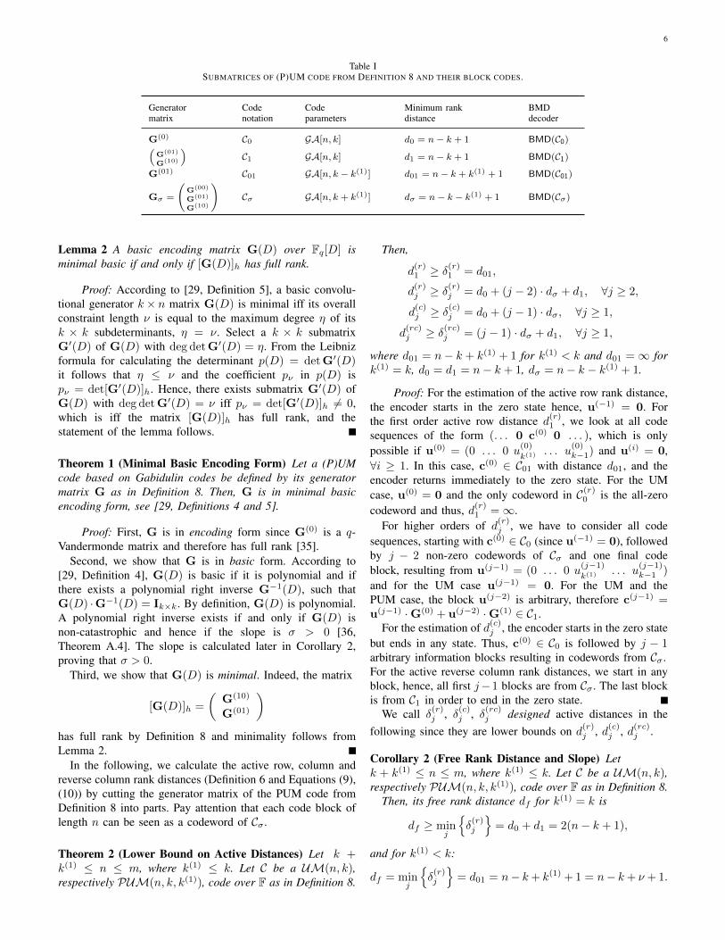
Table I denotes some Gabidulin codes, which are definedby submatrices of G, their minimum rank distances and theirblock rank-metric error-erasure BMD decoders (realized e.g.,by the decoders from [7], [27]). These BMD decoders decodecorrectly if (3) is fulfilled for the corresponding minimum rankdistance. If we consider unit memory codes with k = k(1),then d00 = d10 = n− k + 1, dσ = n− 2k + 1 and d01 =∞,since G(01) does not exist.

To show that the generator matrix G of Definition 8 is inminimal basic encoding form, see [29, Definitions 4 and 5]and [34], let us slightly generalize Theorem 6 from [34] forthe case of arbitrary finite field Fq as follows. Let [G(D)]hbe a matrix over Fq having the leading coefficient of gij(D)in position (i, j) if deg gij(D) = νi and 0 otherwise.

6

Table ISUBMATRICES OF (P)UM CODE FROM DEFINITION 8 AND THEIR BLOCK CODES.

Generatormatrix

Codenotation

Codeparameters

Minimum rankdistance

BMDdecoder

G(0) C0 GA[n, k] d0 = n− k + 1 BMD(C0)(G(01)

G(10)

)C1 GA[n, k] d1 = n− k + 1 BMD(C1)

G(01) C01 GA[n, k − k(1)] d01 = n− k + k(1) + 1 BMD(C01)

Gσ =

(G(00)

G(01)

G(10)

)Cσ GA[n, k + k(1)] dσ = n− k − k(1) + 1 BMD(Cσ)

Lemma 2 A basic encoding matrix G(D) over Fq[D] isminimal basic if and only if [G(D)]h has full rank.

Proof: According to [29, Definition 5], a basic convolu-tional generator k × n matrix G(D) is minimal iff its overallconstraint length ν is equal to the maximum degree η of itsk × k subdeterminants, η = ν. Select a k × k submatrixG′(D) of G(D) with deg det G′(D) = η. From the Leibnizformula for calculating the determinant p(D) = det G′(D)it follows that η ≤ ν and the coefficient pν in p(D) ispν = det[G′(D)]h. Hence, there exists submatrix G′(D) ofG(D) with deg det G′(D) = ν iff pν = det[G′(D)]h 6= 0,which is iff the matrix [G(D)]h has full rank, and thestatement of the lemma follows.

Theorem 1 (Minimal Basic Encoding Form) Let a (P)UMcode based on Gabidulin codes be defined by its generatormatrix G as in Definition 8. Then, G is in minimal basicencoding form, see [29, Definitions 4 and 5].

Proof: First, G is in encoding form since G(0) is a q-Vandermonde matrix and therefore has full rank [35].

Second, we show that G is in basic form. According to[29, Definition 4], G(D) is basic if it is polynomial and ifthere exists a polynomial right inverse G−1(D), such thatG(D) ·G−1(D) = Ik×k. By definition, G(D) is polynomial.A polynomial right inverse exists if and only if G(D) isnon-catastrophic and hence if the slope is σ > 0 [36,Theorem A.4]. The slope is calculated later in Corollary 2,proving that σ > 0.

Third, we show that G(D) is minimal. Indeed, the matrix

[G(D)]h =

(G(10)

G(01)

)has full rank by Definition 8 and minimality follows fromLemma 2.

In the following, we calculate the active row, column andreverse column rank distances (Definition 6 and Equations (9),(10)) by cutting the generator matrix of the PUM code fromDefinition 8 into parts. Pay attention that each code block oflength n can be seen as a codeword of Cσ .

Theorem 2 (Lower Bound on Active Distances) Let k +k(1) ≤ n ≤ m, where k(1) ≤ k. Let C be a UM(n, k),respectively PUM(n, k, k(1)), code over F as in Definition 8.

Then,

d(r)1 ≥ δ(r)

1 = d01,

d(r)j ≥ δ

(r)j = d0 + (j − 2) · dσ + d1, ∀j ≥ 2,

d(c)j ≥ δ

(c)j = d0 + (j − 1) · dσ, ∀j ≥ 1,

d(rc)j ≥ δ(rc)

j = (j − 1) · dσ + d1, ∀j ≥ 1,

where d01 = n− k + k(1) + 1 for k(1) < k and d01 =∞ fork(1) = k, d0 = d1 = n− k + 1, dσ = n− k − k(1) + 1.

Proof: For the estimation of the active row rank distance,the encoder starts in the zero state hence, u(−1) = 0. Forthe first order active row distance d

(r)1 , we look at all code

sequences of the form (. . . 0 c(0) 0 . . . ), which is onlypossible if u(0) = (0 . . . 0 u

(0)

k(1). . . u

(0)k−1) and u(i) = 0,

∀i ≥ 1. In this case, c(0) ∈ C01 with distance d01, and theencoder returns immediately to the zero state. For the UMcase, u(0) = 0 and the only codeword in C(r)

0 is the all-zerocodeword and thus, d(r)

1 =∞.For higher orders of d(r)

j , we have to consider all codesequences, starting with c(0) ∈ C0 (since u(−1) = 0), followedby j − 2 non-zero codewords of Cσ and one final codeblock, resulting from u(j−1) = (0 . . . 0 u

(j−1)

k(1). . . u

(j−1)k−1 )

and for the UM case u(j−1) = 0. For the UM and thePUM case, the block u(j−2) is arbitrary, therefore c(j−1) =u(j−1) ·G(0) + u(j−2) ·G(1) ∈ C1.

For the estimation of d(c)j , the encoder starts in the zero state

but ends in any state. Thus, c(0) ∈ C0 is followed by j − 1arbitrary information blocks resulting in codewords from Cσ .For the active reverse column rank distances, we start in anyblock, hence, all first j−1 blocks are from Cσ . The last blockis from C1 in order to end in the zero state.

We call δ(r)j , δ(c)

j , δ(rc)j designed active distances in the

following since they are lower bounds on d(r)j , d(c)

j , d(rc)j .

Corollary 2 (Free Rank Distance and Slope) Letk + k(1) ≤ n ≤ m, where k(1) ≤ k. Let C be a UM(n, k),respectively PUM(n, k, k(1)), code over F as in Definition 8.

Then, its free rank distance df for k(1) = k is

df ≥ minj

{δ

(r)j

}= d0 + d1 = 2(n− k + 1),

and for k(1) < k:

df = minj

{δ

(r)j

}= d01 = n− k+ k(1) + 1 = n− k+ ν + 1.

7

The slope σ of C for both cases is:

σ ≥ limj→∞

{δ

(r)j

j

}= dσ = n− k − k(1) + 1.

Thus, for any k(1) < k, the construction attains the upperbound on the free rank distance of PUM codes (12). Whenk(1) = k = 1, we attain the upper bound on the free rankdistance of UM codes, see (11). For k(1) = 1 ≤ k, the upperbound on the slope is attained.

If we compare this to the construction from [21], we seethat both constructions attain the upper bound on the free rankdistance for k(1) < k. It depends on the explicit values of n,k and k(1), which construction has a higher slope.

The construction based on the parity-matrix from [21]requires that R = k/n ≥ µH/(µH + 1), where µH ≥ 1,and provides therefore a high-rate code construction, whereasthe construction based on the generator matrix (Definition 8)results in a low-rate code since k + k(1) ≤ n has to hold.

B. Construction of Arbitrary Code Rate

In the sequel, we outline how to extend the constructionfrom Definition 8 to arbitrary code rates. Compared to thehigh-rate construction from [21], the advantage is that weare able to decode this code construction efficiently (see Sec-tion V). We apply the same strategy to extend the constructionfrom Definition 8 to arbitrary code rates as in [33] in Hammingmetric. Further, we use the same notations for the matrices asin the previous section, but with an additional prime symbolfor each matrix (e.g., G becomes G′).

So far, we have defined the code Cσ as a GA[n, k + k(1)]code with dσ = n − k − k(1) + 1, where k + k(1) ≤ n (seealso Table I). Overcoming the restriction k + k(1) ≤ n wouldenable us to choose an arbitrary code rate R = k/n of theconvolutional code C for any fixed k(1). However, at the sametime, if k+k(1) > n, there have to be linearly dependent rowsin(

G(0)′

G(1)′

).

Therefore, we define these matrices such that ϕ denotes thenumber of rows which are contained (amongst others) in both,G(0)′ and G(1)′. We define a full-rank (k+k(1)−ϕ)×n matrixG′all by

G′all =

AΦ

G(01)′

B

, (16)

where A and B are in F(k(1)−ϕ)×n, Φ is in Fϕ×n andG(01)′ ∈ F(k−k(1))×n such that G′all is a generator matrixof a GA[n, k + k(1) − ϕ] code of minimum rank distancedall = d′σ = n− k − k(1) + ϕ+ 1. Clearly, k + k(1) − ϕ ≤ nand d′σ ≤ n have to hold. Since G′all defines a Gabidulin code,any submatrix of consecutive rows defines a Gabidulin codeas well. Based on the definition of G′all, our generalized PUMcode construction is given as follows.

Definition 9 (Generalized (P)UM Code Construction) Letk+k(1)−ϕ ≤ n ≤ m, where ϕ < k(1) ≤ k. Further, let G′all

be as in (16), defining an GA[n, k+ k(1)−ϕ] code. Our ratek/n (P)UM code is defined by the following submatrices:

G(0)′ =

(G(00)′

G(01)′

)=

AΦ

G(01)′

, G(1)′ =

(G(10)′

0

)=

ΦB0

,(17)

where 0 is the all-zero matrix. We restrict ϕ < k(1) sinceotherwise all rows of G(1)′ are rows of G(0)′. Further, anycode rate k/n in combination with any k(1) is feasible withthis restriction since k+ 1 ≤ k+ k(1)−ϕ ≤ n and hence, wehave only the trivial restriction k < n.

Theorem 3 The generator matrix G′(D) = G(0)′ + G(1)′Dfrom Definition 9 of the Generalized (P)UM code is in minimalbasic encoding form.

Proof: The proof is similar to the one of Theorem 1. Thematrix G′ is minimal as the matrix

[G′(D)]h =

ΦB

G(01)′

has full rank by Definition 9, since it is a submatrix ofgenerator matrix of a Gabidulin code, and minimality followsfrom Lemma 2.

To calculate the active distances of the generalized codeconstruction from Definition 9, we need to take into accountthat consecutive non-zero information blocks can result in zerocode blocks due to the linear dependencies in the rows of G(0)′

and G(1)′. This is shown in the following example.

Example 1 (Zero Code Block) Let two consecutive infor-mation blocks u(j−1), u(j) ∈ Fk be:

u(j−1) = (u(j−1)0 . . . u

(j−1)ϕ−1 0 . . . 0),

u(j) = (0 . . . 0 u(j)

k(1)−ϕ . . . u(j)

k(1)−10 . . . 0).

By encoding c(j), we obtain

c(j) = u(j) ·

AΦ

G(01)′

+ u(j−1) ·

ΦB0

=(

(u(j)

k(1)−ϕ . . . u(j)

k(1)−1) + (u

(j−1)0 . . . u

(j−1)ϕ−1 )

)·Φ.

If (u(j)

k(1)−ϕ . . . u(j)

k(1)−1) = −(u

(j−1)0 . . . u

(j−1)ϕ−1 ), we obtain

an all-zero code block c(j) = 0 although u(j−1),u(j) 6= 0.

However, in the same way as in [33, Lemma 1], it can beshown that the maximum number of consecutive zero blocksis bounded from above by ` = dϕ/(k(1)−ϕ)e. Hence, after atmost ` zero code blocks, there has to be (at least) one non-zerocode block and the slope can be lower bounded by

σ′ ≥ d′σ`+ 1

=n− k − k(1) + ϕ+ 1

d k(1)

k(1)−ϕe. (18)

8

This provides the following extended distances:

d(r)′1 ≥ δ(r)′

1 = d01, (19)

d(r)j ≥ δ

(r)′j = d0 + (j − 2) · σ′ + d1, ∀j ≥ 2,

d(c)′j ≥ δ(c)′

j = d0 + (j − 1) · σ′, ∀j ≥ 1,

d(rc)′j ≥ δ(rc)′

j = (j − 1) · σ′ + d1, ∀j ≥ 1,

which reduces to the distances of Theorem 2 for ` = 0. Notethat d0, d01 and d1 are independent of ϕ and therefore thesame as in Table I. We see that there is a trade-off betweenthe code rate and the extended distances; namely, the higherthe code rate, the higher ϕ (for fixed k(1)), and the lower σ′

and the lower the extended distances (for constant ϕ− k).

V. ERROR-ERASURE DECODING OF PUM GABIDULINCODES

This section provides an efficient error-erasure decodingalgorithm for our construcion of (P)UM codes as in Defini-tion 8, using the block rank-metric decoders of the underlyingGabidulin codes in Table I. We explain the general idea,prove its correctness and show how to generalize the decodingalgorithm to the arbitrary-rate construction from Definition 9.

A. Bounded Row Distance Condition and Decoding Algorithm

We consider the terminated generator matrix of a (P)UMcode as in (4) and therefore, each codeword has lengthN + µ = N + 1. Let the received sequence r = c + e =(r(0) r(1) . . . r(N)) ∈ Fn(N+1) be given and let the matrixsequence R = (R(0) R(1) . . . R(N)) ∈ Fm×n(N+1)

q denotethe matrix representation of r, where R(i) = Φβ

(r(i)),

∀i ∈ [0, N ].Let R(i) = C(i) + E(i), for all i ∈ [0, N ], where R(i) ∈

Fm×nq can be decomposed as in (2), including t(i) errors, %(i)

row erasures and γ(i) column erasures in rank metric.Analog to Justesen’s definition in Hamming metric [16], we

define a bounded (row rank) distance decoder for convolutionalcodes in rank metric, incorporating additionally erasures.

Definition 10 (BRD Error–Erasure Decoder) Given a re-ceived sequence r = c + e ∈ Fn(N+1), a bounded rowdistance (BRD) error-erasure decoder in rank metric for aconvolutional code C guarantees to find the code sequencec ∈ C if

i+j−1∑h=i

(2 · t(h) + %(h) + γ(h)

)< δ

(r)j , (20)

∀i ∈ [0, N ], j ∈ [0, N − i+ 1],

where t(h), %(h), γ(h) denote the number of errors, row andcolumn erasures in block E(h) = Φβ

(e(h)

)∈ Fn as in (2).

In Algorithm 1, we present such a BRD rank-metric error-erasure decoder for (P)UM codes constructed as in Defini-tion 8. It is a generalization of the Dettmar–Sorger algorithm[22] to rank metric and to error-erasure correction. The gen-eralization to error-erasure decoding can be done in a similarway in Hamming metric.

The main idea of Algorithm 1 is to take advantage of thealgebraic structure of the underlying block codes and theirefficient decoders (see Table I). We use the outputs of theseblock decoders to build a reduced trellis, which has only veryfew states at every depth. As a final step of our decoder, thewell-known Viterbi algorithm is applied to this reduced trellis.Since there are only a few states in the trellis, the Viterbialgorithm has quite low complexity.

The first step of Algorithm 1 is to decode r(i), ∀i ∈[1, N − 1], with BMD(Cσ), since each code block c(i) is acodeword of Cσ , ∀i ∈ [1, N − 1]. This decoding is guaranteedto be successful if 2t(i) + %(i) + γ(i) < dσ . Because of thetermination, the first and the last block can be decoded in thecodes C0 and C01, respectively, which have a higher minimumrank distance than Cσ . Let c(i)′, for all i ∈ [0, N ], denote theresult of this decoding when it is successful.

Algorithm 1.c← BOUNDEDROWDISTANCEDECODERPUM

(r)

Input: Received sequencer = (r(0) r(1) . . . r(N)) ∈ Fn(N+1)

q

1 Step 1: Decode r(0) with BMD(C0)2 Decode r(i) with BMD(Cσ), for all i ∈ [1, N − 1]3 Decode r(N) with BMD(C01)4 Assign metric m(i) as in (21), for all i ∈ [0, N ]

5 Step 2: For all found c(i): decode `(i)f steps forward with6 BMD(C0),7 decode `(i)b steps backward with8 BMD(C1)9 Step 3: For all found c(i): decode r(i+1) with BMD(C01)

10 Assign metric m(i) as in (25), for all i ∈ [0, N ]

11 Step 4: Find complete path with smallest sum rank metric12 using the Viterbi algorithm

Output: Codeword sequencec = (c(0) c(1) . . . c(N)) ∈ Fn(N+1)

For all i ∈ [0, N ], we draw an edge in a reduced trelliswith the following edge metric:

m(i)=

rk(r(i) − c(i)′), if BMD(C0) (i = 0), BMD(Cσ)

(i ∈ [1, N − 1]), BMD(C01) (i = N )successful⌊

dσ+1+%(i)+γ(i)

2

⌋, else. (21)

Notice that the metric for the successful case is alwayssmaller than the metric for the non-successful case since

rk(r(i)−c(i)′) = t(i)+%(i)+γ(i) ≤⌊dσ + 1 + %(i) + γ(i)

2

⌋−1.

If the block error-erasure decoder BMD(Cσ)decodes correctly, the result is c(i)′ = u(i)G(0) +

(u(i−1)0 u

(i−1)1 . . . u

(i−1)

k(1)−1) · G(10). Since the minimum

distance is dσ ≥ 1, we can reconstruct the whole informationvector u(i) = (u

(i)0 u

(i)1 . . . u

(i)k−1) as well as the part of the

previous information vector, i.e., (u(i−1)0 u

(i−1)1 . . . u

(i−1)

k(1)−1).

9

Assume, we reconstructed u(i) and(u

(i−1)0 u

(i−1)1 . . . u

(i−1)

k(1)−1) in Step 1, then we can

calculate:

r(i+1)− (u(i)0 u

(i)1 . . . u

(i)

k(1)−1) ·G(10) = u(i+1)G(0) + e(i+1)

(22)

r(i−1)− (u(i−1)0 u

(i−1)1 . . . u

(i−1)

k(1)−1) ·G(00)

= (u(i−1)

k(1). . . u

(i−1)k−1 | u

(i−2)0 . . . u

(i−2)

k(1)−1)

(G01

G10

)+ e(i−1).

Hence, Step 2 uses the information from block i to decode`(i)f blocks forward with BMD(C0) and `(i)b blocks backward

with BMD(C1) from any node found in Step 1. This closes(most of) the gaps between two blocks correctly decodedby BMD(Cσ) (of course, it is not known, which blocks aredecoded correctly).

We define the values `(i)f and `(i)b as follows:

`(i)f =min

j

(j j∑h=1

(dσ −m(i+h))≥ δ

(c)j −

j∑h=1

(%(i+h) + γ(i+h)

)2

),

(23)

`(i)b = min

j

(j j∑h=1

(dσ −m(i−h))≥ δ

(rc)j −

j∑h=1

(%(i−h) + γ(i−h)

)2

).

(24)

These definitions are chosen such that we can guaranteecorrect decoding if the BRD condition (20) is fulfilled (seeSection V-B).

For Step 3 and some i ∈ [0, N − 1], assume we know(u

(i+1)0 u

(i+1)1 . . . u

(i+1)

k(1)−1) and u(i) from Step 1 or 2, then

as in (22), we can calculate

r(i+1)−(u(i+1)0 . . . u

(i+1)

k(1)−1)·G(00)− (u

(i)0 . . . u

(i)

k(1)−1)·G(10)

= (u(i+1)

k(1)u

(i+1)

k(1)+1. . . u

(i+1)

k(1)−1) ·G(01) + e(i+1),

which shows that we can use BMD(C01) to close a remaininggap in block i+ 1.

After Step 3, assign as metric to each edge

m(i) =

rk(r(i) − c(i)′), if BMD(C0), BMD(C1) or

BMD(C01) successful,⌊d01 + 1 + %(i) + γ(i)

2

⌋, else, (25)

∀i ∈ [0, N ], where c(i)′ denotes the result of a successfuldecoding. For one received block r(i), there can be severaldecoding results c(i)′ from the different BMD decoders. Thus,there can be more than one edge in the reduced trellis atdepth i. Each edge is labeled with regard to (25) using itscorresponding code block.

Finally, we use the Viterbi algorithm to find the path ofsmallest sum rank weight in this reduced trellis. As in [22],we use m(i), for all i ∈ [0, N ], as edge metric and the sumover different edges as path metric. The different steps of ourdecoding algorithm are roughly summarized in Algorithm 1,the details can be found in the preceding description andFigure 4 illustrates our decoding algorithm.

In Section V-B, we prove that if (20) is fulfilled, then afterthe three block decoders, all gaps are closed and the Viterbialgorithm finds the path with the smallest sum rank weight.

B. Proof of Correctness

In the following, we prove that decoding with Algorithm 1is successful if the BRD condition (20) is fulfilled. The prooffollows the proof of Dettmar and Sorger [22], [36]. Lemma 3shows that the gaps between two correct results of Step 1 arenot too big and Lemmas 4 and 5 show that the gap size afterSteps 1 and 2 is at most one if the BRD condition (20) isfulfilled. Theorem 4 shows that these gaps can be closed withBMD(C01) and the Viterbi algorithm finds the correct path.

Lemma 3 (Gap Between two Correct Results of Step 1)If the BRD condition (20) is satisfied, then the length of anygap between two correct decisions in Step 1 of Algorithm 1,denoted by c(i), c(i+j), is less than min{L(i)

f , L(i)b }, where

L(i)f =min

j

(j j∑h=1

(dσ −m(i+h))≥δ

(r)j −

j∑h=1

(%(i+h) + γ(i+h))

2

),

L(i)b =min

j

(j j∑h=1

(dσ −m(i−h))≥δ

(r)j −

j∑h=1

(%(i−h) + γ(i−h))

2

).

Proof: Decoding of a block r(i) in Step 1 fails or outputsa wrong result if there are at least (dσ − %(i) − γ(i))/2 errorsin rank metric. In such a case, the metric m(i) = b(dσ + 1 +%(i) + γ(i))/2c is assigned.

In order to prove the statement, assume there is a gap of atleast L(i)

f blocks after Step 1. Then,

L(i)f∑

h=1

t(i+h) ≥L

(i)f∑

h=1

dσ − %(i+h) − γ(i+h)

2≥

L(i)f∑

h=1

(dσ −m(i+h)

)

≥δ

(r)

L(i)f

−L

(i)f∑

h=1

(%(i+h) + γ(i+h)

)2

,

which follows from the definition of the metric (21) and fromthe definition of L(i)

f . This contradicts the BRD condition (20).Similarly, we can prove this for L(i+j)

b and hence, the gap sizehas to be less than min{L(i)

f , L(i)b }.

Note that L(i)f and `

(i)f differ only in using the active

row rank distance δ(r)j and the active column rank distance

δ(c)j , respectively. Further, Lemma 3 will not be used in the

following, but it shows an upper bound on the size of the gapsbetween two correctly decoded blocks after the first step ofour decoding algorithm.

Lemma 4 (Correct Path for Few Errors) Let c(i) andc(i+j) be decoded correctly in Step 1 of Algorithm 1. LetStep 2 of Algorithm 1 decode `(i)f blocks in forward directionstarting in c(i), and `

(i+j)b blocks in backward direction

starting in c(i+j) (see also (23), (24)).

10

r(0) . . . r(i) r(i+1) r(i+2) r(i+3) r(i+4) . . .Given:

Step 1:BMD(Cσ)

c(0) . . .BMD(C0)

c(i+2) c(i+4) . . .

Step 2:BMD(C0),BMD(C1)

c(0) . . . c(i+2) c(i+4)c(i+1) c(i+3)

. . .. . .. . .

Step 3:BMD(C01)

c(0) . . . c(i+2) c(i+3)c(i+1) c(i+4)c(i)

. . .

. . .

Step 4:

Viterbi

Figure 4. Illustration of the different steps of Algorithm 1: The received sequence (r(0) r(1) . . . r(N)) is given and the different steps and their decodingresults are shown. Dashed blocks/edges illustrate that they were found in a previous step.

Then, the correct path is in the reduced trellis if the BRDcondition (20) is satisfied and if in each block less thanmin{(d0 − %(i) − γ(i))/2, (d1 − %(i) − γ(i))/2} rank errorsoccurred.

Proof: If there are less thanmin

{(d0 − %(i) − γ(i))/2, (d1 − %(i) − γ(i))/2

}errors

in a block, BMD(C0) and BMD(C1) always yield the correctdecision. Due to the definition of `(i)f , see (23), the forwarddecoding with BMD(C0) terminates as soon as

`(i)f∑h=1

t(i+h) ≥`(i)f∑h=1

dσ − %(i+h) − γ(i+h)

2≥

`(i)f∑h=1

(dσ −m(i+h)

)

≥δ

(c)

`(i)f

−`(i)f∑h=1

(%(i+h) + γ(i+h)

)2

=d0

2+(`(i)f − 1

)dσ2−∑`

(i)f

h=1

(%(i+h) + γ(i+h)

)2

,

where the first inequality holds since the decoding result couldnot be found in Step 1 and the second and third hold due tothe definition of the metric (21) and the definition of `(i)f .

Similarly, backward decoding with BMD(C1) terminates if

`(i+j)b∑h=1

t(i+j−h) ≥d1

2+(`(i+j)b − 1

)dσ2

−∑`

(i+j)b

h=1

(%(i+j−h) + γ(i+j−h)

)2

.

The correct path is in the reduced trellis if `(i)f +`(i+j)b ≥ j−1,

since the gap is then closed. Assume now on the contrary that`(i)f + `

(i+j)b < j − 1. Since Step 1 was not successful for the

blocks in the gap, at least (dσ − %(h) − γ(h))/2 rank errorsoccured in every block r(h), ∀h ∈ [i+ `

(i)f +1, i+ j− `(i+j)b −

1], i.e, in the blocks in the gap between the forward and thebackward path. Then,

j−1∑h=1

t(i+h) ≥δ

(c)

`(i)f

−∑`(i)f

h=1(%(i+h) + γ(i+h))

2

≥`(i)f∑h=1

t(i+h)+

`(i+j)b∑h=1

t(i+j−h)+

j−1−`(i+j)b∑h=`

(i)f +1

dσ − %(i+h) + γ(i+h)

2

≥ d0

2+(`(i)f − 1

)dσ2−

`(i)f∑h=1

(%(i+h) + γ(i+h))

2

+d1

2+(`(i+j)b − 1

)dσ2−

`(i+j)b∑h=1

(%(i+j−h) + γ(i+j−h)

)2

+

(j − 1− `(i)f − `

(i+j)b

)2

dσ −

j−1−`(i+j)b∑h=`

(i)f +1

(%(i+h) + γ(i+h)

)2

≥ d0

2+d1

2+

(j − 3)

2dσ −

∑j−1h=1

(%(i+h) + γ(i+h)

)2

=δ

(r)j−1 −

∑j−1h=1

(%(i+h) + γ(i+h)

)2

,

which is a contradiction to the BRD condition (20) and thestatement follows.

Lemma 5 (Gap Size is at Most One After Steps 1 and 2)Let c(i) and c(i+j) be decoded correctly in Step 1 of

11

Algorithm 1 (with no other correct decisions in between) andlet the BRD condition (20) be fulfilled. Let d0 = d1.

Then, there is at most one error block e(h), h ∈ [i+ 1, i+j − 1], of rank at least (d0 − %(i) − γ(i))/2.

Proof: To fail in Step 1, there have to be at least (dσ −%(i)−γ(i))/2 errors in r(i), ∀i ∈ [i+ 1, i+ j−1]. If two errorblocks in this gap have rank at least (d0− %(i)− γ(i))/2, then

j−1∑h=1

t(i+h) ≥ 2 · d0

2+ (j − 3) · dσ

2−

j−1∑h=1

(%(i+h) + γ(i+h)

)2

≥δ

(r)j−1

2−∑j−1h=1

(%(i+h) + γ(i+h)

)2

,

which contradicts (20).Lemmas 4 and 5 show that if the BRD condition is satisfied,then the correct path is in the reduced trellis after Steps 1 and2, except for at most one block.

Theorem 4 (Correct Path is in Reduced Trellis) If theBRD condition (20) is satisfied, then the correct path is inthe reduced trellis after Step 3 of Algorithm 1.

Proof: Lemmas 4 and 5 guarantee that after Step 2, atmost one block of the correct path is missing in the reducedtrellis. For one block, say r(h), it follows from the BRDcondition that (2 · t(h) + %(h) + γ(h)) < δ

(r)1 = df and any

decoder of distance at least δ(r)1 is able to decode correctly in

this block. Hence, after Step 3, BMD(C01) is able to find thecorrect solution for this block since d01 = δ

(r)1 and the correct

path is in the reduced trellis.The complexity is determined by the complexity of the

BMD rank block error-erasure decoders from Table I, whichare all in the order O(n2) operations in F. Hence, the calcu-lation of the complexity of Algorithm 1 is straight-forward to[22, Theorem 3] and we can give the following bound on thecomplexity without proof.

Theorem 5 (BRD Decoding with Algorithm 1) Letk + k(1) ≤ n ≤ m, where k(1) ≤ k. Let C be azero-forced terminated UM(n, k) or PUM(n, k, k(1))code over F as in Definition 8. Let a received sequencer = (r(0) r(1) . . . r(N)) ∈ Fn(N+1) be given.

Then, Algorithm 1 finds the code sequence c =(c(0) c(1) . . . c(N)) ∈ Fn(N+1) with smallest sum rankdistance to r if the BRD condition from (20) is satisfied.The complexity of decoding one block of length n is at mostO(dσn

2) ≤ O(n3) operations in F.

C. Decoding of the Arbitrary-Rate Code Construction

For the arbitary-rate code construction from Section IV-B,our decoding algorithm from the previous section can bemodified straight-forward to [33]. Hence, we outline thisadaption only shortly here and refer the reader to [33] fordetails.

The linear dependencies in the matrices G(0)′ and G(1)′

(see Definition 9) have the effect that ` consecutive zero blocks

within the code sequence are possible (compare Section IV-B).Further, the dependencies spread the information to ` + 1blocks and we can therefore guarantee to reconstruct a certaininformation block u(i) only if ` + 1 consecutive blocks(including code block u(i)) could be decoded. This is shownin the following example.

Example 2 (Reconstructing Information Block) Let ϕ =2k(1)/3, where ` = 2 and Φ has twice as much rows as A.Assume, we have decoded c(0), c(1) and c(2) and we want toreconstruct u(1).

We decompose u(0),u(1),u(2) into sub-blocks, i.e.: u(j) =

(u(j)1 | u(j)

2 | u(j)3 | u(j)

4 ) for j = 0, 1, 2, where the first threesub-blocks have length k(1) − ϕ and the last sub-block haslength k − k(1). Then,

c(1) = (u(1)1 | u

(1)2 + u

(0)1 | u

(1)3 + u

(0)2 | u

(1)4 | u

(0)3 )·

AΦ1

Φ2

G(01)′

B

def= u(1) ·G′all,

where Φ =(

Φ1

Φ2

)and Φ1, Φ2 each have k(1) − ϕ rows.

Since we know c(1), and since G′all defines an MRD code,we can reconstruct the vector u(1). This directly gives usu

(1)1 and u

(1)4 . This reconstruction can be done in the same

way for c(0) and we obtain (amongst others) u(0)1 . To obtain

u(1)2 , we subtract u

(0)1 from the known sum u

(1)2 + u

(0)1 . The

reconstruction for c(2) provides u(1)3 and we have recovered

the whole information block u(1).This example has shown why ` + 1 consecutive decoded

blocks are necessary to reconstruct one information block. Itdoes not matter if the other decoded blocks precede or succeedthe required information block.

Apart from the reconstruction of the information, there arefurther parts in the decoding algorithm which have to bemodified. An error of minimum weight causing a sequenceof non-reconstructible information blocks in the first decodingstep has the following structure:

(0, . . . , 0,×︸ ︷︷ ︸`+1 blocks

| 0, . . . , 0,×︸ ︷︷ ︸`+1 blocks

| . . . | 0, . . . , 0,×︸ ︷︷ ︸`+1 blocks

| 0, . . . , 0︸ ︷︷ ︸` blocks

),

where × marks blocks (of length n) of rank weight at leastdσ/2. In this case, also the information of the ` error-freeblocks between the erroneous blocks cannot be reconstructedsince we need `+1 consecutive decoded blocks to reconstructthe information. Further, the last ` error-free blocks make itnecessary to decode ` additional steps in forward direction inthe second step of Algorithm 1.

In order to decode with Algorithm 1, we have to take intoaccount the slower increase of the resulting extended distancesdue to the sequences of possible zero code blocks. Hence, asin [33], we generalize (23) by simply subtracting ` in thesummation, which is equivalent to going ` steps further:

12

`(i)′f =min

j

(jj−`∑h=1

d′σ −m(i+h)

`+ 1≥δ(c)′j −

j∑h=1

(%(i+h) + γ(i+h)

)2

),

(26)which reduces to (23) for ` = 0. Further `(i)′b = `

(i)b .

Hence, in order to decode the arbitrary-rate construction wehave to modify Algorithm 1 as follows:• the reconstruction of information blocks requires ` + 1

consecutive code blocks as in Example 2,• the path extension `(i)f has to be prolonged as in (26),• the metric definitions in (21), (25) have to be modified

by simply adding “and u(i) could be reconstructed” inthe if-part of both definitions.

Then, as in Section V-B, we can guarantee that the correctpath is in the reduced trellis if

i+j−1∑h=i

(2 · t(h) + %(h) + γ(h)

)< δ

(r)′j ,

∀i ∈ [0, N ], j ∈ [0, N − i+ 1],

where δ(r)′j is defined as in (19).

VI. APPLICATION TO RANDOM LINEAR NETWORKCODING

Our motivation for considering convolutional codes in rankmetric is to apply them in multi-shot random linear networkcoding (RLNC). In this section, we first explain the modelof multi-shot network coding and show how to define lifted(P)UM codes in rank metric. Afterwards, we show howdecoding of these lifted (P)UM codes reduces to error-erasuredecoding of (P)UM codes in rank metric.

A. Multi-Shot Transmission of Lifted PUM Codes

As network channel model we assume a multi-shot transmis-sion over the so-called operator channel. The operator channelwas defined by Kotter and Kschischang in [6] and the conceptof multi-shot transmission over the operator channel was firstconsidered by Nobrega and Uchoa-Filho [11].

In this network model, a source transmits packets (whichare vectors over a finite field) to a sink. The network hasseveral directed links between the source, some internal nodesand the sink. The source and sink apply coding techniques forerror control, but have no knowledge about the structure of thenetwork. This means, we consider non-coherent RLNC. In amulti-shot transmission, we use the network several times andthe internal structure may change in every time instance. Indetail, we assume that we use it N+1 times. In the following,we shortly give basic notations for this network channel model.The notations are similar to [7], but we include additionallythe time dependency.

Let X(i) ∈ Fn×(n+m)q , ∀i ∈ [0, N ]. The rows represent

the transmitted packets X(i)0 , X

(i)1 , . . . , X

(i)n−1 ∈ Fn+m

q at time

instance (shot) i. Similarly, let Y(i) ∈ Fn(i)×(n+m)q be a

matrix whose n(i) rows correspond to the received packetsY

(i)0 , Y

(i)1 , . . . , Y

(i)

n(i)−1∈ Fm+n

q . Notice that n and n(i) do not

have to be equal since packets can be erased and/or additionalpackets might be inserted.

The term random linear network coding originates fromthe behavior of the internal nodes: they create random linearcombinations of the packets received so far in the currentshot i, ∀i ∈ [0, N ]. Additionally, erroneous packets might beinserted into the network and transmitted packets might be lostor erased.

Let the links in the network be indexed from 0 to `−1, then,as in [7], let the rows of a matrix Z(i) ∈ F`×(n+m)

q containthe error packets Z(i)

0 , Z(i)1 , . . . , Z

(i)`−1 inserted at the links 0

to `− 1 at shot i. If Z(i)j = 0, j ∈ [0, `− 1], then no corrupt

packet was inserted at link j ∈ [0, ` − 1] and time i. Due tothe linearity of the network, the output can be written as:

Y(i) = A(i)X(i) + B(i)Z(i), (27)

where A(i) ∈ Fn(i)×nq and B(i) ∈ Fn(i)×`

q are the (unknown)channel transfer matrices at time i.

When there are no errors or erasures in the network, the rowspace of Y(i) is the same as the row space of X(i). In [6], [7]it was shown that subspace codes constructed by lifted MRDcodes (as in Lemma 1) provide an almost optimal solutionto error control in the operator channel. Such lifted MRDcodes are a special class of constant-dimension codes (seeLemma 1). In the following, we define lifted PUM codes basedon Gabidulin codes in order to use these constant-dimensioncodes for error correction in multi-shot network coding.

Definition 11 (Lifted (Partial) Unit Memory Code) Let Cbe a zero-forced terminated UM(n, k) or PUM(n, k, k(1))code over F as in Definition 8. Represent each code blockc(i) ∈ Fn, ∀i ∈ [0, N ], as matrix C(i) = Φβ

(c(i))∈ Fm×nq .

Then, the lifting of C is defined by the following set ofsubspace sequences:

lift(C) def={(Rq([In C(0)T ]

). . . Rq

([In C(N)T ]

)):(

Φ−1β (C(0)) . . . Φ−1

β (C(N)))∈ C}.

As in Definition 2, we denote lift(C(i)T ) = Rq([In C(i)T ]

),

∀i ∈ [0, N ]. We transmit this sequence of subspaces over theoperator channel such that each transmitted matrix is a liftedblock of a codeword of the rank-metric PUM code, i.e., X(i) =[In C(i)T ], ∀i ∈ [0, N ]. Of course, any other basis of the rowspace can also be chosen as transmitted matrix.

By means of this lifted PUM code, we create dependenciesbetween the different shots in the network. Since each codeblock of length n is a codeword of the block code Cσ , eachtransmitted subspace is a codeword of a CDq(n + m, dS =2dσ, n) constant-dimension code, lying in Gq(n + m,n), see[7, Proposition 4] and Lemma 1. However, the lifted (P)UMcode contains additionally dependencies between the differentblocks and for decoding, we obtain therefore a better perfor-mance than simply lifting the block code Cσ as in Lemma 1.Since the PUM code transmits k information symbols per shot,a comparison with a lifted block code of rate k/n is muchfairer than comparing it with Cσ (see also Example 3).

13

B. Decoding of Lifted PUM Codes in the Operator Channel

In this section, we will show how the decoding problemin the operator channel reduces to error-erasure decoding ofPUM codes based on Gabidulin codes—analog to [7], whereit reduces to error-erasure decoding of Gabidulin codes. Sinceeach code block of length n of a PUM(n, k, k(1)) code isa codeword of the block code Cσ , we can directly use thereformulations of Silva, Kschischang and Kotter [7].

Let the transmitted matrix at time instance i be X(i) =[In C(i)T ] and denote by Y(i) = [A(i) Y(i)] ∈ Fn

(i)×(n+m)q

the received matrix after the multi-shot transmission over theoperator channel as in (27). The channel transfer matrices A(i)

and B(i) are time-variant. Moreover, assume rank(Y(i)) =n(i), since linearly dependent received packets are directlydiscarded. Then, as in [7], we denote the column and rowdeficiency of A(i) by:

γ(i) def= n−rank(A(i)), %(i) def

= n(i)−rank(A(i)), ∀i ∈ [0, N ].

If we calculate the reduced row echelon (RRE) form of Y(i)

(and fill it up with zero rows, if necessary), we obtain thefollowing matrix in F(n+%(i))×(n+m)

q (similar to [7, Proposi-tion 7], but in our notation):

RRE0

(Y(i)

)=

(In + B(i,C)T ITU(i) R(i)T

0 A(i,R)T

), (28)

for a set U (i) ⊆ [0, n − 1] with |U (i)| = γ(i) such thatITU(i)R

(i)T = 0 and ITU(i)B(i,C)T = −Iγ(i) , and IU(i) denotes

the submatrix of In consisting of the columns indexed by U (i).Moreover, B(i,C)T ∈ Fn×γ(i)

q and A(i,R)T ∈ F%(i)×nq .

Furthermore, it was shown in [7] that R(i) can be decom-posed into

R(i) = C(i) + A(i,R)B(i,R) + A(i,C)B(i,C) + A(i,E)B(i,E),

∀i ∈ [0, N ], where(Φ−1

β (C(0)) . . . Φ−1β (C(N))

)∈ C

and A(i,R) and B(i,C) are known to the receiver, since thematrix from (28) can be calculated from the channel output.Comparing this equation to (2) makes clear that the problemof decoding lifted PUM codes (as in Definition 11) in theoperator channel reduces to error-erasure decoding of the PUMcode in rank metric. For this purpose, we can use our decodingalgorithm from Section V, which is based on rank-metric error-erasure block decoders.

Now, let the received matrix sequence Y =(Y(0) Y(1) . . . Y(N)) as output of the operator channelbe given, then Algorithm 2 shows how to reconstruct thetransmitted information sequence.

Algorithm 2.u← NETWORKPUMDECODER

(Y)

Input: Received sequence Y = (Y(0) Y(1) . . . ,Y(N)),

where Y(i) ∈ Fn(i)×(n+m)q , ∀i ∈ [0, N ]

1 γ(i) ← n− rank(A(i)), ∀i ∈ [0, N ]

2 %(i) ← n(i) − rank(A(i)), ∀i ∈ [0, N ]

3 Calculate RRE0(Y(i)) and R(i) as in (28), ∀i ∈ [0, N ]

4 r = (r(0) . . . r(N))←(Φ−1

β (R(0)) . . . Φ−1β (R(N))

)5 c = (c(0) c(1) . . . c(N))←

BOUNDEDROWDISTANCEDECODERPUM(r)

withAlgorithm 1

6 Reconstruct u = (u(0) u(1) . . .u(N−1))

Output: Information sequenceu = (u(0) u(1) . . .u(N−1)) ∈ FkN

The asymptotic complexity of Algorithm 2 for decodingone matrix Y(i) of size n(i) × (n + m) scales cubic in nover F. Calculating the RRE is at most cubic in n overFq if we use Gaussian elimination. However, Algorithm 1has asymptotic complexity O(n3) over F, which dominatestherefore the complexity of Algorithm 2. The reconstruction ofthe information sequence from the code sequence is negligible.

Example 3 (Lifted PUM Code for Network Coding) LetN + 1 = 7, n = 8 ≤ m, k = 4, k(1) = 2 and therefored0 = d1 = 5, d01 = 7 and dσ = 3 (Table II). Let C bea PUM(n, k, k(1)) code as in Definition 8. Construct thelifting of C as in Definition 11.

Assume, Y = (Y(0) Y(1) . . . Y(6)) is given as output ofthe operator channel and apply Algorithm 2.

After calculating the RRE (and filling the matrix with zerorows as in (28)), let the number of errors, row erasures andcolumn erasures in each block be as in Table II. The results ofthe different decoding steps of Algorithm 1 for error-erasuredecoding of PUM codes are also shown. In this examplethe BRD condition (20) is fulfilled and correct decoding istherefore guaranteed due to Theorem 5.

The code rate of C is 1/2 and as a comparison with the(lifted) Gabidulin codes from [7], the last line in Table IIshows the decoding of a block Gabidulin code of rate 1/2 andminimum rank distance d = 5. For fairness, the last block isalso decoded with a GA[8, 2] code. The block decoder fails inShots 1 and 5.

However, similar to the ongoing discussion whether block orconvolutional codes are better, it depends on the distributionof the errors and erasures, i.e., on the channel, whether theconstruction from [7] or ours performs better.

VII. APPLICATION TO RANDOM AFFINENETWORK CODING

In this section, we outline the application of our constructionof (P)UM codes in rank metric to error control in randomaffine network coding (RANC), introduced by Gadouleau andGoupil in [5]. In this model, the transmitted packets areregarded as points in an affine space and the network performs

14

Table IIEXAMPLE FOR ERROR-ERASURE DECODING OF LIFTED (PARTIAL) UNIT MEMORY CODES BASED ON GABIDULIN CODES.

Shot i 0 1 2 3 4 5 6

%(i) + γ(i) 0 1 3 1 1 0 2

t(i) 2 2 0 1 0 3 2

PUM code Decoding with Cσ ,block 0 with C0,block N with C10

X× × × X ×

XDecoding with C0, C1 × X X ×Decoding with C01 X X

Block code Decoding with GA[8, 4] X × X X X × X

affine linear combinations of the received packets, i.e., the sumof the coefficients included in the linear combination equalsone. Instead of (linear) subspace codes, affine subspace codesare considered, i.e., a code is a set of affine subspaces of anaffine space, where an affine subspace of dimension r is alinear subspace of dimension r−1, which is translated by onepoint. RANC increases the data rate by around one symbol perpacket compared to RLNC. For details, the reader is referredto [5].

Similar to the linear lifting of Definition 2, an affinelifting can be used to construct affine subspace codes. Theaffine lifting of a code C is defined as follows: Let Ir−1 =

[0 Ir−1]T ∈ Fr×(r−1)q , where 0 = (0 0 . . . 0)T ∈ F(r−1)×1

q .Then, the subspace lifta(X) = Rq

([Ir−1 X]

)denotes the

affine lifting of X ∈ Fr×(n−r+1)q . Compared to the linear

lifting (Definition 2), the overhead is reduced by one columnand the size of X is increased by r symbols, which makesaffine lifting more efficient than linear lifting.

Based on the definition of affine lifting, we can immedi-ately consider the affine lifting of our (P)UM code C fromDefinition 11 by the following set of spaces:

lifta(C) def={(Rq([In−1 C(0)T ]

). . . Rq

([In−1 C(N)T ]

)):(

Φ−1β (C(0)) . . . Φ−1

β (C(N)))∈ C},

where In−1 = [0 In−1]T ∈ Fn×(n−1)q and therefore the

overhead is reduced by one column compared to Definition 11.Alternatively, we can also define C such that C(i) ∈ F(m+1)×n

q ,then the transmitted space has the same size as for RLNC, butwe transmit n additional information symbols over Fq .

As shown in [5, Section VI], the decoding of affine liftedcodes is not more complicated than the one of linear liftedcodes and, for our construction, it reduces in a similar way asin Section VI to error-erasure decoding of the (P)UM code.

VIII. CONCLUSION

In this paper, we have considered convolutional codes inrank metric, their decoding and their application to randomlinear network coding.

First, we have shown general distance measures for con-volutional codes based on a modified rank metric—the sumrank metric—and have recalled upper bounds on the free rank

distance and the slope of (P)UM codes based on the sumrank metric. Second, we have given an explicit constructionof (P)UM codes based on the generator matrices of Gabidulincodes and have calculated its free rank distance and slope.This (low-rate) construction achieves the upper bound on thefree rank distance. We have also generalized this constructionto arbitrary code rates. Third, we have presented an efficienterror-erasure decoding algorithm for our (P)UM construction.The algorithm guarantees to correct errors up to half the activerow rank distance and its complexity is cubic in the length.Finally, we have shown how constant-dimension codes, whichwere constructed by lifting the (P)UM code, can be appliedfor error control in random linear network coding and outlinedthe application of (P)UM codes in rank metric to affine linearnetwork coding.

ACKNOWLEDGMENT

The authors would like to thank Martin Bossert, AlexanderZeh, and Victor Zyablov for the valuable discussions and thereviewers for their very helpful comments.

REFERENCES

[1] A. Wachter-Zeh and V. Sidorenko, “Rank Metric Convolutional Codesfor Random Linear Network Coding,” in IEEE Int. Symp. NetworkCoding (Netcod), Jul. 2012.

[2] R. Ahlswede, N. Cai, S. Li, and R. Yeung, “Network Information Flow,”IEEE Trans. Inform. Theory, vol. 46, no. 4, pp. 1204–1216, Aug. 2000.

[3] T. Ho, R. Kotter, M. Medard, D. R. Karger, and M. Effros, “The Benefitsof Coding over Routing in a Randomized Setting,” in IEEE Int. Symp.Inf. Theory (ISIT), Jun. 2003, p. 442.

[4] T. Ho, M. Medard, R. Kotter, D. R. Karger, M. Effros, J. Shi, andB. Leong, “A Random Linear Network Coding Approach to Multicast,”IEEE Trans. Inform. Theory, vol. 52, no. 10, pp. 4413–4430, Oct. 2006.

[5] M. Gadouleau and A. Goupil, “A Matroid Framework for Noncoher-ent Random Network Communications,” IEEE Trans. Inform. Theory,vol. 57, no. 2, pp. 1031–1045, Feb. 2011.

[6] R. Kotter and F. R. Kschischang, “Coding for Errors and Erasures inRandom Network Coding,” IEEE Trans. Inform. Theory, vol. 54, no. 8,pp. 3579–3591, Jul. 2008.

[7] D. Silva, F. R. Kschischang, and R. Kotter, “A Rank-Metric Approachto Error Control in Random Network Coding,” IEEE Trans. Inform.Theory, vol. 54, no. 9, pp. 3951–3967, 2008.

[8] P. Delsarte, “Bilinear Forms over a Finite Field with Applications toCoding Theory,” J. Combin. Theory Ser. A, vol. 25, no. 3, pp. 226–241,1978.

[9] E. M. Gabidulin, “Theory of Codes with Maximum Rank Distance,”Probl. Inf. Transm., vol. 21, no. 1, pp. 3–16, 1985.

[10] R. M. Roth, “Maximum-Rank Array Codes and their Application toCrisscross Error Correction,” IEEE Trans. Inform. Theory, vol. 37, no. 2,pp. 328–336, 1991.

15

[11] R. W. Nobrega and B. F. Uchoa-Filho, “Multishot Codes for NetworkCoding Using Rank-Metric Codes,” in IEEE Wireless Network CodingConf. (WiNC), Jun. 2010, pp. 1–6.

[12] L.-N. Lee, “Short Unit-Memory Byte-Oriented Binary ConvolutionalCodes Having Maximal Free Distance,” IEEE Trans. Inform. Theory,pp. 349–352, May 1976.

[13] G. S. Lauer, “Some Optimal Partial-Unit Memory Codes,” IEEE Trans.Inform. Theory, vol. 23, no. 2, pp. 240–243, Mar. 1979.

[14] V. V. Zyablov and V. R. Sidorenko, On Periodic (Partial) Unit MemoryCodes with Maximum Free Distance, ser. Lecture Notes in ComputerScience, 1994, vol. 829, pp. 74–79.

[15] F. Pollara, R. J. McEliece, and K. A. S. Abdel-Ghaffar, “Finite-StateCodes,” IEEE Trans. Inform. Theory, vol. 34, no. 5, pp. 1083–1089,1988.

[16] J. Justesen, “Bounded Distance Decoding of Unit Memory Codes,” IEEETrans. Inform. Theory, vol. 39, no. 5, pp. 1616–1627, 1993.

[17] U. Dettmar and U. K. Sorger, “New Optimal Partial Unit Memory Codesbased on Extended BCH Codes,” Electronics Letters, vol. 29, no. 23,pp. 2024–2025, Nov. 1993.

[18] U. Dettmar and S. Shavgulidze, “New Optimal Partial Unit MemoryCodes,” Electronic Letters, vol. 28, pp. 1748–1749, Aug. 1992.

[19] C. Thommesen and J. Justesen, “Bounds on Distances and ErrorExponents of Unit Memory Codes,” IEEE Trans. Inform. Theory, vol. 29,no. 5, pp. 637–649, 1983.

[20] A. Wachter, V. Sidorenko, M. Bossert, and V. Zyablov, “Partial UnitMemory Codes Based on Gabidulin Codes,” in IEEE Int. Symp. Inf.Theory (ISIT), Aug. 2011, pp. 2487–2491.

[21] A. Wachter, V. R. Sidorenko, M. Bossert, and V. V. Zyablov, “On(Partial) Unit Memory Codes Based on Gabidulin Codes,” Probl. Inf.Transm., vol. 47, no. 2, pp. 38–51, 2011.

[22] U. Dettmar and U. K. Sorger, “Bounded Minimum Distance Decodingof Unit Memory Codes,” IEEE Trans. Inform. Theory, vol. 41, no. 2,pp. 591–596, 1995.

[23] E. Erez and M. Feder, “Convolutional Network Codes,” in IEEE Int.Symp. Inf. Theory (ISIT), Jun. 2004, p. 146.

[24] S. Y. R. Li and R. W. Yeung, “On Convolutional Network Coding,” inIEEE Int. Symp. Inf. Theory (ISIT), Jul. 2006, pp. 1743–1747.

[25] K. Prasad and B. S. Rajan, “On Network-Error Correcting ConvolutionalCodes Under the BSC Edge Error Model,” in IEEE Int. Symp. Inf. Theory(ISIT), Jun. 2010, pp. 2418–2422.

[26] W. Guo, N. Cai, X. Shi, and M. Medard, “Localized Dimension Growthin Random Network coding: A Convolutional Approach,” in IEEE Int.Symp. Inf. Theory (ISIT), Jul. 2011, pp. 1156–1160.

[27] E. M. Gabidulin and N. I. Pilipchuk, “Error and Erasure CorrectingAlgorithms for Rank Codes,” Des. Codes Cryptogr., vol. 49, no. 1-3,pp. 105–122, 2008.

[28] R. Johannesson and K. S. Zigangirov, Fundamentals of ConvolutionalCoding. Wiley-IEEE Press, 1999.

[29] G. D. Forney, “Convolutional Codes I: Algebraic Structure,” IEEE Trans.Inform. Theory, vol. 16, no. 6, pp. 720–738, 1970.

[30] S. Host, R. Johannesson, K. S. Zigangirov, and V. V. Zyablov, “Ac-tive Distances for Convolutional Codes,” IEEE Trans. Inform. Theory,vol. 45, no. 2, pp. 658–669, Mar. 1999.

[31] R. Jordan, V. Pavlushkov, and V. V. Zyablov, “Maximum Slope Con-volutional Codes,” IEEE Trans. Inform. Theory, vol. 50, no. 10, pp.2511–2526, 2004.

[32] R. Jordan, “Design Apects of Woven Convolutional Coding,” Ph.D.dissertation, Ulm University, Ulm, Germany, Apr. 2002.

[33] A. Wachter-Zeh, M. Stinner, and M. Bossert, “Efficient Decoding ofPartial Unit Memory Codes of Arbitrary Rate,” in IEEE Int. Symp. Inf.Theory (ISIT), Jul. 2012, pp. 2356–2360.

[34] R. Johannesson and Z.-X. Wan, “A Linear Algebra Approach to MinimalConvolutional Encoders,” IEEE Trans. Inform. Theory, vol. 39, no. 4,pp. 1219–1233, Jul. 1993.

[35] R. Lidl and H. Niederreiter, Finite Fields, ser. Encyclopedia of Mathe-matics and its Applications. Cambridge University Press, Oct. 1996.

[36] U. Dettmar, “Partial Unit Memory Codes,” Ph.D. dissertation, Universityof Darmstadt, Darmstadt, Germany, Jun. 1994.