TERRESTRIAL LASER SCANNING METRIC CONTROL:

ASSESSMENT OF METRIC ACCURACY FOR CULTURAL HERITAGE MODELING

J. G. Lahoza, D.G. Aguileraa, J. Finatb, J. Martíneza/b, J. Fernándezb and J. San Joséb

aIMAP3D Group, Land and Cartography Engineering Department, Univ. of Salamanca, Spain, fotod@usal.es

bDAVAP Group, Lab.2.2, Building I+D, Univ. of Valladolid, Spain ,jfinat@agt.uva.es KEY WORDS: Cultural Heritage, Laser scanning, Accuracy, Metric Control. ABSTRACT: This contribution gives account of one of the results achieved by the group MAPA (Models and Algorithms for the digital documentation of Architectural Heritage) that integrates the IMAP3D group and the DAVAP group. The group work is based on the assumption that preservation of cultural heritage is a responsibility for the whole cartographic community and that the recent advances in Digital Image Processing, Photogrammetry and Computer Graphics provide efficient tools for the digital documentation and visualization of the Cultural Heritage. The increasing availability of devices for 3D acquisition in digital format can be used to build very precise models of 3D objects in an effective and fast way and with a low personal cost. The aim of the group is to develop algorithms to test, process, integrate and visualize data acquired from singular historical buildings by means of a 3D laser scanner or by means of photogrammetric or surveying procedures. More specifically, through this paper we address the assessment of the accuracy of the 3D Laser Scanner while documenting a particular historical building: the church of "San Nicolás" in Ávila (Spain). To achieve so we have designed, developed and measured a control geodetic network, assessed the accuracy and reliability related to it and, finally, compared the coordinates obtained through the laser scanner with the coordinates obtained through the surveying process. The plan of the paper is, firstly, to establish the background of our work; then, to describe briefly the target building; next, to describe the sensors involved; afterwards, to describe the geodetic network and the methodology used to measure and adjust it, present the experimental results and, finally, summarize some relevant conclusions.

1. INTRODUCTION

There is no doubt that the 3D laser scanner has changed greatly the data acquisition process in disciplines that go from Surveying and Photogrammetry to Architecture, Civil Engineering, Industry and even Criminology. Nevertheless, its most outstanding feature - the fast, massive and automatic capture of 3D metric information - has its own drawbacks. On one hand, we have to deal with huge amounts of points, which demand very competitive processors. Besides this, information is obtained in a scan procedure, i.e. in a non selective way in which blunders or irrelevant information is mixed with the proper information. Points acquired show no structure at all. Even more, the singular points which express the object geometry may not have been captured at all. These factors must be managed in a several stations procedure in which we must adjust data clouds and in which we run the risk to be exposed to error propagation if orientation within point sets is approached in a consecutive way. These considerations highlight the need to develop a protocol in which we can asses the quality in a building model obtained by means of a 3D laser scanner. Specifically, our task was to control the accuracy of a model of the Church of San Nicolás in Ávila, obtained by means of Trimble GS200 laser scanner in a seven station sequence. To achieve this we have chosen an adequate surveying instrument - a Leica TPS 1000 total station - we have designed and measured a geodetic network integrated by 8 stations and 18 control points, we have adjusted it and assessed, applying the classical Least Squares criterion together with Baarda and Pope tests - style statistical procedures - and,

finally, we have compared the results obtained by the two sensors and methods.

2. THE CHURCH OF SAN NICOLAS

The origins of the church of San Nicolás (Figure 1) date back to the early days of the repopulation of Castille, a fact supported by an inscription which shows that its devotion to San Nicolás, the Bishop, took place in 1198. It is right in the middle of the Moorish quarter, 200 m outside the City Walls, and the poverty of its materials reflects in some way the poverty of its former parishioners.

Figure 1. Church of San Nicolás (Ávila)

From the outside it can be seen that the church has a single apse, a tower and two doors. The tower has three decreasing sections, and was built in two different periods, which explains why the access staircase is spiral in the first section, and made of wood supported by the walls in the upper half. Apparently, it never had bells.

The church is 30 m long (east-west direction), 22 m wide and 12 m tall in the central part with a maximum height at the tower with 24 m. This fact leads to an extra laser station, away enough of church in order to scan the upper part of the tower due to the limited scanning vertical range of Trimble GS200 (40º above the horizon). It is formed by a three naves main body, articulated with the apse, the tower and a minor construction devoted to the sacristy. It shows the typical romanic style absence of ornamentation except for the two doorways. They are placed at the north and south facades with five and two archivolts respectively and the also usual decorative motives that demand a higher resolution scan. The main nave exhibits four buttresses in its occidental part. The church is in the middle of a city garden and so, it makes easier to surround it and place the laser scanner or whatever sensor. The church is relatively well preserved, i.e. it shows a high regularity in its surfaces geometry and radiometry. On the side of the drawbacks, we may talk of a dense “curtain” of trees which occlude part of the facades. Both on the east and north parts, buildings are too close to the church to allow a flexible design of the geodetic network. On the west there is a high traffic street while at the east there is a quiet street but full of middle size vehicles parked there.

3. SENSOR DESCRIPTION

The 3D laser scanner Trimble GS200 has a 360º horizontal field of view while the vertical field ranges from 40º above horizon to 20º below horizon. The calibration certificate guarantees a 2.3 mm error at a distance of 25 meters and a 1.6 mm error related to a distance of 50 meters. Distances measured at the workspace were between these two thresholds. Maximum errors are expected to be of 3 mm for both distances. It has a resolution of 3 mm at 100 m and a speed of 5000 points per second. For the geodetic work, a Leica TPS 1000 total station was chosen due to its high capabilities: 0.5" angular accuracy and 1 mm + 1 ppm distances accuracy. It is also endowed with automatic correction of collimation error, vertical index, eccentricity, earth curvature and refraction. It was complemented with the Leica mini-prism in the measuring of distances. In addition to the low resolution camera placed within de laser scanner, a Nikon D70 of 3008 x 2000 pixels with a 14 mm focal length was used to acquire texture for the further renderization of the model.

Figure 2. 3D laser scanner Trimble GS200, Leica TPS 1000 total station and the Leica mini-prism

4. METRIC CONTROL METHODOLOGY

The geodetic network design was based on the following basic principles. The main objectives of a network design are:

To achieve an accuracy and reliability fixed beforehand.

To apply reliability controls based on statistical tests and on robust estimators to avoid any misleading due to gross errors.

To choose acceptable measuring procedures under practical and economical conditions.

According to this, the designing procedure will include the following steps:

Selection of appropriate instruments and measuring techniques.

Localization and assessment of every station in the network.

Specification of every possible observation.

To manage redundant observations a functional and a stochastic model are to be specified. The first one, to express the geometric idealized relations at the basis of the network and the second one, to express the uncertainty associated to the measuring task. So, we will use the Gauss-Markov Model to adjust our model with three types of equations, as usual: one for the observed distances, one for the observed horizontal angles and one more for the observed vertical angles. Every observation will provide an equation and as long as we will use the two first terms of the Taylor Theorem to linearize the model, the unknowns will be the corrections to be applied to the initial approximations.

The output of this procedure, as is well known, is the adjusted coordinates of the points in the network and the residuals or corrections of the observations, as well as the estimation of the accuracy and reliability associated to them. This result is based on the normal distribution hypothesis and is derived from the application of the error propagation principles expressed through the jacobian and the covariance matrix. The linearized functional model is in the form: AX-L=V, where X is the vector of unknowns, corrections to the initial approximations; L is the vector of observations and V is the vector of corrections to the observations. The weight matrix is defined as: W = σo

2Σll, where Σll is the covariance matrix of the observations that embrace distances, horizontal angles and vertical angles. The adjustment criterion is and leads to the solution:

where r is the redundancy in the adjustment. So, the model is fed by an input which has a basic geometric component (design matrix A) and a basic metric component (weight matrix W). The model provides as output:

• A vector of adjusted corrections to the initial coordinate approximations of the points: X

• A vector of adjusted residuals or corrections of the

observations: V

• A covariance matrix of the latter , that expresses, mainly through the terms in the principal diagonal an estimation of the accuracy of the solution.

• A covariance matrix of the adjusted residuals, ,

that contains, in the terms of principal diagonal, the redundancy numbers, i.e. an indication of the network robustness and so, a measure of the reliability of the solution.

• Statistical tests that asses the model global validity

(such as Chi2 test) and that detect gross errors (such as Baarda and Pope test).

In synthesis, three factors are addressed in the network design: 1. The instrument precision, reflected on the covariance matrix of the observations and, consequently on the weight matrix W. 2. The network geometry, reflected on the design matrix A. 3. Observation redundancy, reflected on √r factor that appears in the mean square error. We obtain the appropriate feedback through the covariance matrices of the unknowns and the residuals. According to Fraser (Fraser, 1987), the conceptual flow of the network design may be expressed as follows (Figure 3):

Figure 3. Network design scheme According to the previous concepts the network was designed as follows: A Leica total station TPS 1000 was chosen due to its high precision both in angles and distances. A Leica mini-prism was also chosen as a competitive complement of the former. It was decided to measure as much distances and angles as possible between whatever two network stations. The environment geometrical restrictions led to refuse the design of a double ring stations that would have produced a higher

WLAtWAANtNX

T

T

=

=

= −1

122^ −==∑ NQ oXXoXXσσ

rPVVAAQQQQ

TT

XXllVVVVoVV=−==∑ 2

02^ σσ

MínPVV T →=φ Precision and reliability criteria

Instrument selection Basic geometry configuration

Establish geometry (Matrix A)

Enough Precision?

END

Enough with scaling ?

Number of observations

Enough with changing

geometry?

Yes

No

Yes

Yes

No

No

∑ XX̂

∑VV̂

redundancy. Both to guarantee a trisection on the control points on the facades and to avoid an excessive reduction of the distances between the stations, a basic eight vertex figure was assumed as shown in Figure 4. This configuration provides a redundancy of 220 that seemed initially to be enough.

Figure 4. Eight vertex design of the network 18 control points to test the laser scanner accuracy were placed on the facades: four points were placed at the each of the short facades (east and west) and five at each of the long ones. For this purpose, we decided to use the targets provided by the laser scanner Trimble GS200 (Figure 5) in order to ease point cloud merging.

Figure 5. Target used as tie point for the point cloud merging, as well as control point

The scanning design was established on two basic principles:

Minimum station number to avoid multi station orientation procedures but enough station number to guarantee a global coverage of all surfaces and taking into account obstructions due to the presence of trees or cars.

Station settlement aiming at an optimization of the incidence ray angle at the façade, as well as a harmonization between the most efficient scanning distance accuracy (approximately 40 meters according to instrument specifications) and most efficient distance coverage (especially due to the limited vertical scanning range).

To ease the cloud merging procedure to a unique datum and to make this datum consistent with the geodetic one, we decided to use the control targets provided within the laser scanner Trimble GS200. Eighteen targets provided by the laser scanner Trimble GS200 were placed at the facades. As is explained before, these targets had a double mission: to facilitate the cloud merging process and to provide the basic framework for the comparison of the results achieved by the scanning procedure and by the geodetic one.

5. EXPERIMENTAL RESULTS

The scanning process at each station consisted on the acquisition of a low resolution RGB image with the scanner camera in order to manage the areas to be scanned and also to project the image texture on the point cloud. Measurement of target points used both to merge the diverse point clouds and to exert the geodetic control. Scanning of the correspondent building surfaces. The average parameters of this task were a 30 x 30 mm resolution for an average distance of 30 m. The post-processing of data included:

• Cloud point depuration applying spatial and topographic filters to eliminate overlapping areas and to erase noisy information. Manual segmentations were also applied to eliminate those features that were not eliminated by the filters.

• A semiautomatic register of the multiple clouds based

on the previous observation of the control targets. To achieve so, the iterative closest point algorithm (ICP) was applied.

• Georeferenciation of the total point cloud in the

geodetic network coordinate system. This process gave a final global error of 13 mm.

• Adjustment of the geodetic network applying the

Gauss Markov Model and applying Chi2, Baarda and Pope tests. No blunder at all was detected through these tests.

• Metric control of the scanner laser through a

dimensional analysis by a comparison of distances between every two control points. This task provided

a global average discrepancy between the laser scanner distances and the geodetic distances of 13 mm and a maximum discrepancy of 44 mm.

The adjustment of the geodetic network gave the precision figures collected in table 1 and in table 2. Station σx (m) σy(m) σz(m)

V1 0.000 0.002 -0.001 V2 -0.001 0.003 -0.000 V3 0.002 -0.004 0.001 V4 -0.002 0.001 0.002 V5 0.003 -0.001 -0.000 V6 0.001 0.003 -0.003 V7 -0.002 -0.002 0.001

Table 1. Standard deviation errors of the network stations Control Point

σx(m) σy(m) σz(m)

N1 -0.002 0.002 -0.000 N2 0.001 0.003 0.001 N3 0.002 0.001 0.003 N4 -0.003 -0.003 -0.001 N5 0.001 -0.000 0.005 S1 0.000 -0.003 0.004 S2 0.002 0.002 0.003 S3 -0.003 -0.003 -0.002 S4 -0.002 -0.004 -0.002 S5 0.001 0.004 -0.003 E1 -0.001 -0.005 0.002 E2 -0.003 -0.001 -0.001 E3 0.005 0.002 0.001 E4 0.003 0.001 -0.003 W1 -0.002 -0.003 0.005 W2 -0.001 -0.002 -0.005 W3 0.003 0.003 0.003 W4 -0.001 -0.003 -0.002

Table 2. Standard deviation errors of the control points

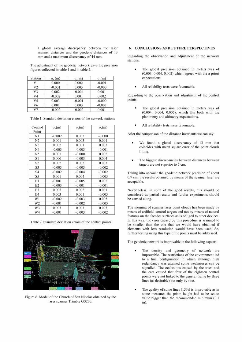
Figure 6. Model of the Church of San Nicolas obtained by the laser scanner Trimble GS200.

6. CONCLUSIONS AND FUTURE PERSPECTIVES

Regarding the observation and adjustment of the network stations:

• The global precision obtained in meters was of (0.003, 0.004, 0.002) which agrees with the a priori expectations.

• All reliability tests were favourable.

Regarding to the observation and adjustment of the control points:

The global precision obtained in meters was of (0.004, 0.004, 0.005), which fits both with the planimetry and altimetry expectations.

All reliability tests were favourable.

After the comparison of the distance invariants we can say:

• We found a global discrepancy of 13 mm that coincides with mean square error of the point clouds fitting.

• The biggest discrepancies between distances between

targets are not superior to 5 cm.

Taking into account the geodetic network precision of about 0.7 cm, the results obtained by means of the scanner laser are acceptable. Nevertheless, in spite of the good results, this should be considered as partial results and further experiments should be carried along. The merging of scanner laser point clouds has been made by means of artificial control targets and not by means of natural features on the facades surfaces as is obliged to other devices. In this way, the error caused by this procedure is assumed to be smaller than the one that we would have obtained if elements with less resolution would have been used. So, further testing using this type of tie points must be addressed. The geodetic network is improvable in the following aspects:

• The density and geometry of network are improvable. The restrictions of the environment led to a final configuration in which although high redundancy was attained some weaknesses can be signalled. The occlusions caused by the trees and the cars caused that four of the eighteen control points were not linked to the general frame by three lines (as desirable) but only by two.

• The quality of some lines (15%) is improvable as in

some measures the prism height had to be set to value bigger than the recommended minimum (0.1 m).

The density and distribution of the control points is improvable. Only 18 points were fixed to the facades due to time restrictions (the scanner laser observations and the surveying observations had to be carried along in the same day). This limitations suggest that further experiments should be addressed choosing an object and an environment in which the conditions can be controlled more closely. This object could be the building of the High Polytechnic School of Avila. On it a network with more and better distributed stations could be designed in which more and better control points could be settled distributed in both natural points and artificial targets. In addition, in this context redundancy could also be augmented by the repetition of measures as time restrictions could be minimized. Unfortunately, this would be an interesting case but not a natural case as these excessively controlled conditions are not met by natural objects placed at natural environments. So, the interest of these further proofs is only partial as the objective of our group is to determine the accuracy that laser scanner can attain under ordinary conditions and not under extraordinary conditions. Nevertheless, the artificial context would be appropriate to examine some critical factors of laser scanner quality. Some of these are:

• Perpendicularity of light rays that conditions both the scanning density as well as precision in distances.

• Average distance from the device station to object

depending on the scanner laser specifications.

• The presence / absence of geometrically well defined elements that allow (or not) a straightforward identification in cross referencing of point clouds.

• Object radiometric resolution that on some scanners

facilitate the cross referencing of point clouds.

• Number of device stations as a critical factor is orientation is transmitted in a sequential fashion. If point clouds are adjusted in a global way (aerotriangulation) this factor should be controllable but if they are oriented in a step by step procedure, errors would accumulate non linearly as a function of the number of stations.

7. REFERENCES

References from Journals: E. P. Baltsavias: A comparison between Photogrammetry and laser scanning. ISPRS Journal of Photogrammetry & Remote Sensing 54_1999.83–94. W. Boheler and A. Marbs: 3D Scanning and Photogrammetry for Heritage Recording: a comparison. Geoinformatics 2004.

Fraser C.S. 1987 "Limiting error propagation in network design". Photogrammetric engineering and remote sensing. 53 (5). 487 - 493. References from Books: W.F. Caspary, “Concepts of Network and Deformation Analysis”. Monografía 11, School of Surveying, The University of New South Wales, Kensington, N.S.W., Australia. Marzo de 1987. Chueca Pazos M. y otros. Redes Topográficas y locales. Microgeodesia. Tomo III. Editorial Paraninfo S.A. Fraser C.S. 1995. "Network design" Close range photogrammetry and Machine Vision. (Ed. Atkinson, K.B.) Whittles Publishing. London Kraus, K. 1997. Photogrammetry. V2. Ümmler. Bonn Mikhail E.M. 1976. "Observations and Least Squares" University press of America. New York.