Improving Data Hiding by Using Convolutional Codes and

Soft-Decision Decoding

Juan R. Hernandez, Jean-Francois Delaigle and Benoıt Macq

ABSTRACT

This paper presents an other way of considering watermarking methods, which are analyzed from thepoint of view of the Information Theory. Watermarking is thus a communication problem in which someinformation bits have to be transmitted through an additive noise channel subjected to distortions andattacks. Designing watermarking methods in such a way that this channel is Gaussian can be profitable.This paper shows to what extent error protection techniques extensively studied for digital communicationthrough Gaussian channels can be used advantageously for watermarking. Convolutional codes combinedwith soft-decision decoding are the best example. Especially, when soft-decision Viterbi decoding is em-ployed, this kind of coding schemes can achieve much better performance than BCH codes, at comparablelevels of complexity and redundancy, both for still and moving images.

1. INTRODUCTION

Watermarking is becoming more and more popular in the scientific literature1,2 as a technology enablingcopyright protection systems. Watermarking is often perceived as a technology providing security systemswith new features, such as content-based authentication3 , playback/copy control4 or detection of copyrightviolation5(i.e. monitoring). In this context, most of the efforts for designing new watermarking algorithms6

or enhancing existing ones7 , are dedicated to the improvement of the robustness. It is obvious thatwatermark messages must be retrieved after the usual processing that are authorized by the author orthe copyright owner. On the contrary, the resistance to malicious attacks is not always required by theapplications that uses watermarking technologies. For such applications, it is more important to maximizethe quantity of information the watermark is able to convey. It is clear that this remark is also relevant inthe case of secure applications but is maybe less crucial. This is why watermarking should also be viewedfrom the angle of the information theory. This is exactly the approach followed in this research work.There are few papers going in that direction8 . Watermarking is analyzed as a communication problemin which some information bits have to be transmitted through an additive noise channel subjected todistortions and attacks. In this communication environment, the original image contents play the role ofadditive noise. Manipulations such as compression and malicious attacks introduce additional noise, linearand non-linear distortions and synchronization mismatches.

This paper is structured as follows. In section 2, an equivalent noisy channel model is obtained by meansof a statistical analysis of the watermarking algorithms employed. Specifically, a low-cost watermarkingalgorithm is studied. As a result of this analysis, an equivalent Gaussian vector channel model is derived.This well-known model allows us to fully characterize the channel by means of the SNR at each channeloutput. One important consequence is that error protection techniques extensively studied for digitalcommunication through Gaussian channels can be used advantageously for watermarking.

In section 3, convolutional codes combined with soft-decision decoding are studied. It is demonstratedthat this kind of coding schemes, when soft-decision Viterbi decoding is employed, can achieve betterperformance than BCH codes, at comparable levels of complexity and redundancy, both for still andmoving images as shown in section 4.

In section 5, all the theoretical analyses will be contrasted with empirical data obtained through sim-ulations. The contribution of this approach is extensively demonstrated through a large set of results.

1

2. EQUIVALENT NOISY VECTOR CHANNEL MODEL

2.1. Watermark Embedding Algorithm

The watermarking algorithm analyzed in this paper operates in the spatial domain, with blocks of 8 � 8pixels. Therefore, the image is first divided in blocks of this size, some of these blocks are selected takinginto account perceptual criteria and then one bit of information is embedded in each block. Let xk[m]

represent the luminance component of the mth pixel of the kth block of the original image intended tobe watermarked. Both pixel and block indexes are, of course, two-dimensional, i.e. m = (m1,m2) andk = (k1, k2). Furthermore, n1, n2 2 f0, . . . , 7g and k1 2 f0, . . . , Lx�1g, k2 2 f0, . . . , Ly�1g, where Lx andLy are the dimensions of the original image measured in 8-pixel blocks. Throughout the rest of the paperwe will use vector notation to represent indexes in two-dimensional signals.

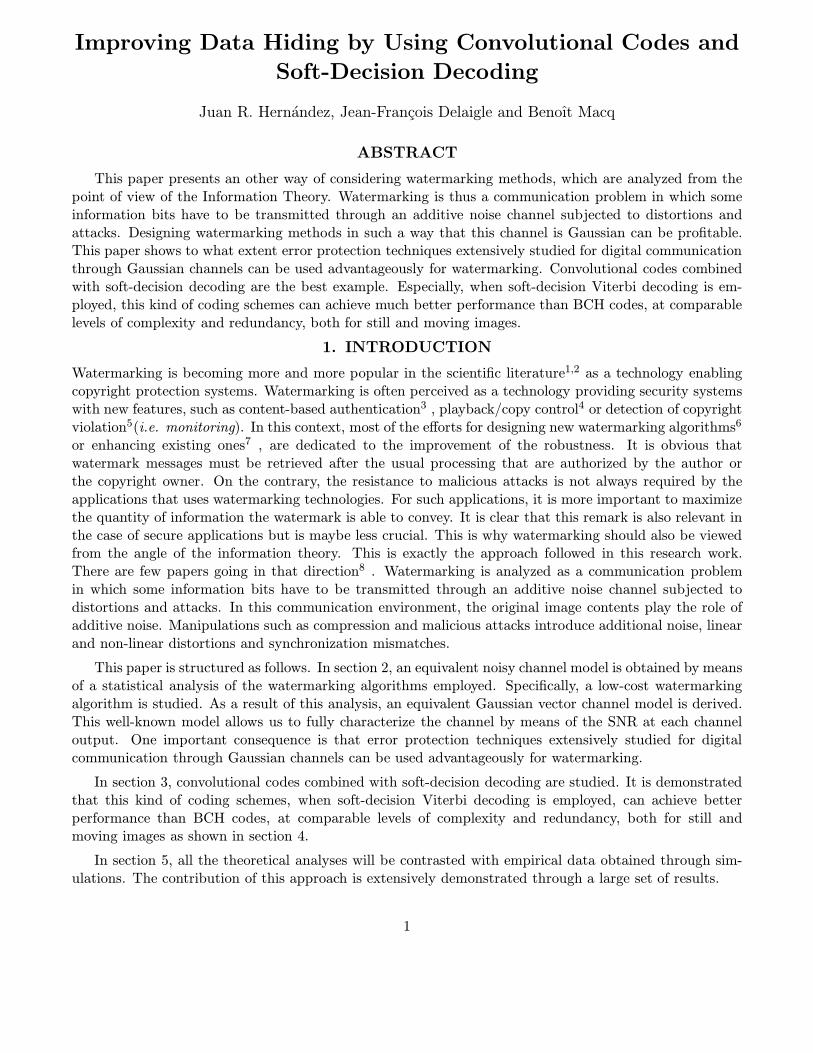
In Fig. 1 we present all the steps involved in the watermark embedding process.9

ENC Replic.BlockEmbed. Deinterl. ny [ ]k

Interl.x [ ]nk

OriginalImage

WatermarkedImage

SecretKey

kc [ ]ny [ ]k

x [ ]nk

b c

CodewordMessage

K

´´

´

Figure 1. Watermark embedding algorithm.

First, an Nu-bit message represented by the binary antipodal vector (b1, . . . , bNu), bi 2 f�1, 1g, 8i 2f1, . . . ,Nug is passed through an encoder, obtaining as a result theNc-bit antipodal coded vector (c1, . . . , cNc),ci 2 f�1, 1g, 8i 2 f1, . . . ,Ncg. Then, this codeword is expanded into a two-dimensional signal c0[k], withthe same size (measured in 8�8-pixel blocks) as the original image, by means of a replication process. Eachreplicated bit is then embedded into the corresponding image block. The original image blocks xk[m] arepassed through an interleaver and the output x0

k[m] is then fed into the bit-by-bit watermark embedder.The interleaving stage can be seen as a two-dimensional pseudo-random permutation of the image blocks.For security purposes, the pseudo-random permutation algorithm depends on the value of a secret key onlyknown by the copyright owner. Using mathematical notation, the relation between the output and theinput of the interleaver can be expressed as x0k[m] = xk0 [m], where k0 = P (K,k), P (�, �) representing a

key-dependent two-dimensional permutation function. From now on, all the names with the 0 symbol willrepresent variables in the interleaved domain. Thanks to the interleaver, an attacker will not be able toknow which information bit is embedded in each image block.

The block-by-block embedding algorithm includes a perceptual analysis process by means of which theblocks where an embedded bit could lead to severe perceptual artifacts are rejected. For the survivingblocks, the power of the embedded watermark is also controlled.9 Each block is divided into two zones(numbered 1 and 2), and each zone is then further subdivided into two categories, A and B. As a result, the64 pixels in each block are classified in four categories (1A, 1B, 2A and 2B). Let S 01A(k), S 01B(k), S 02A(k)and S 02B(k) represent the partition of the set of two-dimensional indexes f0, . . . , 7g � f0, . . . , 7g whichresults after this classification process applied to the kth block x0k[m]. In other words, S 01A(k) contains theindexes m of all the pixels in category 1A, S 01B(k) the indexes of pixels in category 1B, and so on. The

2

classification in categories A and B is performed by using a grid of 8� 8 binary elements. A different gridis taken from a set of predefined grids for each image block. However, the sequence followed for selectingthe grid associated to each block at the output of the interleaver is deterministic and independent of thesecret key.

If c0[k] 2 f�1, 1g is the bit assigned to the k-th 8 � 8 pixel block x0k[m], then the embedding rule forthe pixels in zone 1 is

y0k[m] =

x0k[m] + c0[k]l0[k]

n01B(k)n01A(k)+n

0

1B(k)if m 2 S 01A(k)

x0k[m]� c0[k]l0[k] n01A(k)n01A(k)+n0

1B(k)

if m 2 S 01B(k)(1)

where l0[k] is the embedding level corresponding to the block x0k[m] and n01A(k), n01B(k) are the number

of pixels in categories 1A and 1B respectively in this same block. A similar procedure is followed withzone 2 (categories 2A and 2B). The value of the embedding level is adaptively computed for each block byanalyzing the luminance pixel values.9 If the block is rejected by the perceptual analyser, this is equivalentto setting l0[k] to zero.

Finally, the marked blocks are reordered using a De-interleaver that obtains the inverse of the pseudo-random permutation performed in the interleaver. The relation between the input and the output of theDe-interleaver is yk[m] = y0

k0[m], where k = P (K,k0). Therefore, the embedding rule (1) can also be

expressed directly in the non-interleaved domain as

yk[m] =

xk[m] + c[k]l[k] n1B(k)

n1A(k)+n1B(k)if m 2 S1A(k)

xk[m]� c[k]l[k] n1A(k)n1A(k)+n1B(k)

if m 2 S1B(k)(2)

where c[k] is equal to the sequence c0[k] after being passed through the De-interleaver. In other words,c[k] = c0[k0], where k = P (K,k0). In this new expression of the embedding rule the secret key K onlyaffects the coefficients c[k]. The rest of the terms are key-independent. Note also that the secret key is onlyused in the interleaver and the De-interleaver, so these are the only points in the watermark embeddingalgorithm where secrecy is introduced.

2.2. Watermark Extraction Algorithm

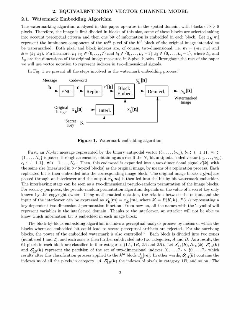
In Fig. 2 we show the different steps involved in the extraction of the watermark contents. The signalzk[m] represents the image intended to be tested, after being divided into 8� 8-pixel blocks as explainedin Section 2.1. It is in general a transformed version of yk[m], after suffering attacks and non maliciousmanipulations.

Σ DECz [ ]nk

ObservedVector

EstimatedMessage

BlockMetricInterl.

SecretKey

br

K

Image

kr [ ]´

Figure 2. Watermark extraction algorithm.

First, the image zk[m] is passed through the same key-dependent interleaver as that shown in Figure1. Then each 8�8-pixel block is processed to obtain a metric r0[k] which is used afterwards when decoding

3

the message carried by the watermark.9 The metric computation includes a perceptual processing stagein which the pixels in each block are classified in zones and categories following the same algorithm asthat used in the watermark embedding process (Sect. 2.1). As a result, for each block z0

k[m] the set of

two-dimensional indexes f0, . . . , 7g � f0, . . . , 7g is partitioned into the sets T 01A(k), T 0

1B(k), T 02A(k) and

T 02B(k). These sets are in general different to those obtained during the embedding process, due to thealterations introduced by the watermark. The metric for the k-th block is defined as9

r0[k] = Σ01[k] + Σ0

2[k], (3)

where

Σ01[k] =

1

n01A(k)

∑m2T 0

1A(k)

z0k[m]� 1

n01B(k)

∑m2T 0

1B(k)

z0k[m] (4)

Σ02[k] =

1

n02A(k)

∑m2T 0

2A(k)

z0k[m]� 1

n02B(k)

∑m2T 0

2B(k)

z0k[m]. (5)

We can see that Σ01[k] is computed as the difference between the average luminance in category 1A and

the average luminance in category 1B. The value Σ02[k] is computed following the same procedure with

categories 2A and 2B. Finally, the metrics r0[k] associated with blocks assigned to a same encoded bit aresummed together in order to obtain a global metric.

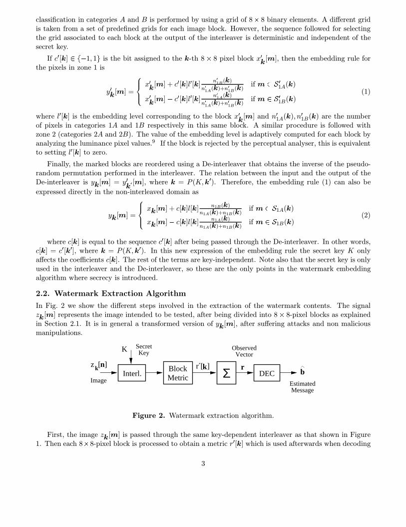
2.3. Equivalent Gaussian Channel

In the transmission chain represented in figures 1 and 2, all the elements between the vector c and thevector of observations r, including the manipulations and malicious attacks that transform yk[m] intozk[m], can be combined together and modeled as an equivalent noisy vector channel (Fig. 3). In thissection we will find a statistical characterization for this channel model, which will be later used whenproposing the convolutional codes and the soft-decision decoder structures.

ENC Channel bc rb

K

DEC

Figure 3. Equivalent Vector Channel Model.

In this paper we are interested in measuring, for a given fixed original image xk[m], the BER (BitError Rate) at the output of the decoder. In other words, we will measure the percentage of keys for whichan error occurs when extracting an arbitrary bit. For this reason, the secret key K will be treated as arandom variable and the original image will be left as a deterministic two-dimensional signal8 .

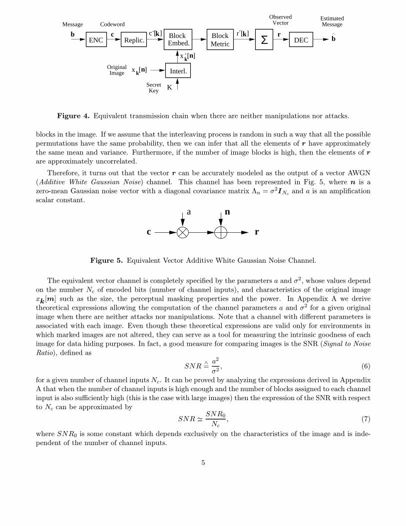
In Figure 4 we have represented the whole chain of processing elements between the message b and theestimate b when the marked image suffers neither attacks nor non-malicious manipulations.

In Fig. 4 we can see that each element of r is the sum of contributions from several 8� 8-pixel blockstaken all over the image. For this reason, if the number of blocks assigned to each encoded bit is sufficientlyhigh (more than 10) then we can apply the central limit theorem and model r as a Gaussian randomvector. In addition, as a consequence of the key-dependent interleaving operation performed before theblock embedding process (see Fig. 1), each element of r takes contributions from pseudorandomly chosen

4

ENC Replic.BlockEmbed.

Interl.

SecretKey K

Σ DEC

ObservedVector

BlockMetric

EstimatedMessage

kc [ ]

x [ ]nk

OriginalImage

x [ ]nk

b c

CodewordMessage

brkr [ ]´

´

´

Figure 4. Equivalent transmission chain when there are neither manipulations nor attacks.

blocks in the image. If we assume that the interleaving process is random in such a way that all the possiblepermutations have the same probability, then we can infer that all the elements of r have approximatelythe same mean and variance. Furthermore, if the number of image blocks is high, then the elements of rare approximately uncorrelated.

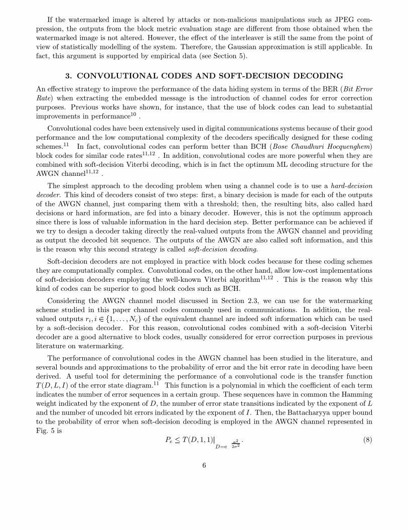
Therefore, it turns out that the vector r can be accurately modeled as the output of a vector AWGN(Additive White Gaussian Noise) channel. This channel has been represented in Fig. 5, where n is azero-mean Gaussian noise vector with a diagonal covariance matrix Λn = σ

2INc and a is an amplificationscalar constant.

a n

c r

Figure 5. Equivalent Vector Additive White Gaussian Noise Channel.

The equivalent vector channel is completely specified by the parameters a and σ2, whose values dependon the number Nc of encoded bits (number of channel inputs), and characteristics of the original imagexk[m] such as the size, the perceptual masking properties and the power. In Appendix A we derivetheoretical expressions allowing the computation of the channel parameters a and σ2 for a given originalimage when there are neither attacks nor manipulations. Note that a channel with different parameters isassociated with each image. Even though these theoretical expressions are valid only for environments inwhich marked images are not altered, they can serve as a tool for measuring the intrinsic goodness of eachimage for data hiding purposes. In fact, a good measure for comparing images is the SNR (Signal to NoiseRatio), defined as

SNR4

=a2

σ2, (6)

for a given number of channel inputsNc. It can be proved by analyzing the expressions derived in AppendixA that when the number of channel inputs is high enough and the number of blocks assigned to each channelinput is also sufficiently high (this is the case with large images) then the expression of the SNR with respectto Nc can be approximated by

SNR ' SNR0Nc

, (7)

where SNR0 is some constant which depends exclusively on the characteristics of the image and is inde-pendent of the number of channel inputs.

5

If the watermarked image is altered by attacks or non-malicious manipulations such as JPEG com-pression, the outputs from the block metric evaluation stage are different from those obtained when thewatermarked image is not altered. However, the effect of the interleaver is still the same from the point ofview of statistically modelling of the system. Therefore, the Gaussian approximation is still applicable. Infact, this argument is supported by empirical data (see Section 5).

3. CONVOLUTIONAL CODES AND SOFT-DECISION DECODING

An effective strategy to improve the performance of the data hiding system in terms of the BER (Bit ErrorRate) when extracting the embedded message is the introduction of channel codes for error correctionpurposes. Previous works have shown, for instance, that the use of block codes can lead to substantialimprovements in performance10 .

Convolutional codes have been extensively used in digital communications systems because of their goodperformance and the low computational complexity of the decoders specifically designed for these codingschemes.11 In fact, convolutional codes can perform better than BCH (Bose Chaudhuri Hocquenghem)block codes for similar code rates11,12 . In addition, convolutional codes are more powerful when they arecombined with soft-decision Viterbi decoding, which is in fact the optimum ML decoding structure for theAWGN channel11,12 .

The simplest approach to the decoding problem when using a channel code is to use a hard-decisiondecoder. This kind of decoders consist of two steps: first, a binary decision is made for each of the outputsof the AWGN channel, just comparing them with a threshold; then, the resulting bits, also called harddecisions or hard information, are fed into a binary decoder. However, this is not the optimum approachsince there is loss of valuable information in the hard decision step. Better performance can be achieved ifwe try to design a decoder taking directly the real-valued outputs from the AWGN channel and providingas output the decoded bit sequence. The outputs of the AWGN are also called soft information, and thisis the reason why this second strategy is called soft-decision decoding.

Soft-decision decoders are not employed in practice with block codes because for these coding schemesthey are computationally complex. Convolutional codes, on the other hand, allow low-cost implementationsof soft-decision decoders employing the well-known Viterbi algorithm11,12 . This is the reason why thiskind of codes can be superior to good block codes such as BCH.

Considering the AWGN channel model discussed in Section 2.3, we can use for the watermarkingscheme studied in this paper channel codes commonly used in communications. In addition, the real-valued outputs ri, i 2 f1, . . . ,Ncg of the equivalent channel are indeed soft information which can be usedby a soft-decision decoder. For this reason, convolutional codes combined with a soft-decision Viterbidecoder are a good alternative to block codes, usually considered for error correction purposes in previousliterature on watermarking.

The performance of convolutional codes in the AWGN channel has been studied in the literature, andseveral bounds and approximations to the probability of error and the bit error rate in decoding have beenderived. A useful tool for determining the performance of a convolutional code is the transfer functionT (D,L, I) of the error state diagram.11 This function is a polynomial in which the coefficient of each termindicates the number of error sequences in a certain group. These sequences have in common the Hammingweight indicated by the exponent of D, the number of error state transitions indicated by the exponent of Land the number of uncoded bit errors indicated by the exponent of I. Then, the Battacharyya upper boundto the probability of error when soft-decision decoding is employed in the AWGN channel represented inFig. 5 is

Pe � T (D, 1, 1)jD=e

�a2

2σ2. (8)

6

And the Battacharyya upper bound to the probability of bit error (BER), when the convolutional codehas a rate k/n, is

Pc �1

k

∂

∂IT (D, 1, I)j

D=e�a2

2σ2 ,I=1. (9)

In the work presented in this paper we have compared the performance of convolutional codes and BCHcodes with similar characteristics. Let us see a theoretical estimate of the BER when BCH block codes areused. In this case, only hard-decision decoding can be employed. The bit error rate at the output of thebit-by-bit hard-decision device can be easily shown to be

Pb = Q(pSNR

). (10)

Then, a good approximation to the BER at the output of the BCH binary block decoder is11

Pc '1

n

n∑m=t+1

m

(n

m

)Pmb (1� Pb)n�m, (11)

where m,n are the number of inputs and outputs respectively, of the block encoder and t is the errorcorrection capacity of the BCH code, i.e. the maximum number of bit errors that it can correct.

An interesting effect it is necessary to take into account when using channel codes for error correctionpurposes is that in general for each coding scheme there is a SNR level below which the code does notintroduce a gain in performance. In fact the BER for this interval of SNR values is worse than in theuncoded case. This effect can be seen graphically if we draw plots of the BER with respect to the SNR(see Section 5). If we do this, we will see that the BER curves for the uncoded and the coded cases havea crossing point at a certain SNR level. This fact might lead us to think that channel codes are of littleinterest. However, this is not true, since the BER for the uncoded case is already very high for SNR valuesbelow this crossing point.

4. EXTENSION TO VIDEO SEQUENCES

We have applied the same watermark embedding algorithm as that presented in Section 2.1 to videosequences. Specifically, the embedding scheme is applied frame by frame, in the spatial non-compresseddomain. The same message is embedded in all the frames, and the interleaver and the grid assignmentprocess are reinitialized for each new frame. In the watermark extraction process, the interleaver and themetric evaluation processes are performed for each frame exactly as explained in Section 2.2. Therefore,now for each frame we have a different vector r = (r1, . . . , rNc). Two different implementations of thedecoder have been tested in for performance comparison purposes.

In the first implementation, based on BCH codes, hard decisions are first performed for all the elementsof all the received vectors. Then, for each of theNc bits, a binary decision is done by majority-logic decodingalong the time axis. The resulting Nc-bit sequence is finally fed into a BCH block decoder. In the sequelwe will call this strategy binary time integration (BTI).

In the second implementation we used convolutional codes combined with soft-decision decoding. Inthis case all the contributions for each of the elements of the soft information vector (r1, . . . , rNc) aresummed together along the time axis by using a discrete-time integrator. Then, the Nc outputs of thebank of integrators are fed into a soft-decision Viterbi decoder. We will call this second scheme simplytime integration (TI).

Results from simulations show that the second implementation is clearly superior in performance. Thisfact is due to two reasons: first, the use of convolutional codes combined with soft-decision decoding leads to

7

better results, even if only one frame is available. Secondly, the mechanism used to combine contributionsfrom different frames is more efficient. In fact, the summation of the outputs of the equivalent AWGNvector channel along the time axis provides sufficient statistics for the decoding problem whenever theoutputs ri from any two different images (for a fixed i) are i.i.d. In practice, this is not the case, and ingeneral the parameters a and σ2 of the equivalent channel will be variable along time. In addition, theoutputs of the equivalent channel will be in general correlated along the time axis due to the intrinsictime correlation of the video contents. Therefore, in general the bank of integrators is not the optimumscheme for combining outputs from different frames. This mechanism, however, is good enough and leadsto better results than the binary time integration approach, as we will see in Section 5. An interesting lineof future research work is the design of computationally efficient methods for estimating the parameters aand σ2 of the equivalent vector channel for each of the frames and then using these estimates for weightingsoft-information contributions from different frames, in such a way that the overall SNR is optimized.

When applied to watermarking of video sequences, channel codes have an additional advantage: theycan reduce considerably the time needed to extract the embedded message with a certain desired level ofperformance in terms of bit error rate (BER). Let us consider first the soft-information time integrationscheme. If we think in terms of the AWGN channel model described in Section 2.3, it is clear that theoutputs of the bank of integrators can also be seen as outputs from an equivalent AWGN channel. In orderto achieve a target BER the equivalent channel must have a least a certain minimum SNR level. If thesoft information samples for each index i 2 f1, . . . ,Ncg can be modeled as outputs from an i.i.d. Gaussianrandom process, then the SNR at the output of the bank of integrators increases linearly with the numberof frames. The coding gain associated with the coding scheme used for error protection will allow us toreduce the SNR necessary to achieve a certain BER. Therefore, the number of frames needed can also bereduced. For instance, if the coding scheme introduces a coding gain of 3 dB, then the number of framesrequired can be reduced to one half.

5. EXPERIMENTAL RESULTS

In order to assess the improvement in performance associated with the use of convolutional codes combinedwith soft-decision decoding strategies, and in order to validate the accurateness of the Gaussian channelmodel and the theoretical approximations to the channel parameters derived in Section A, we have per-formed tests with four images, shown in Figure 6. These test images have been chosen considering theirdiffering characteristics in terms of presence of sharp edges, noisy textures, etc.

In Figure 7 we show histograms of the equivalent channel outputs when a symbol ci = 1 is introduced.We can see in the first plot, corresponding to the case in which the watermarked image is not altered, thatthe histogram has a Gaussian shape. The other two plots represent histograms of the soft informationwhen the watermarked image is compressed using the JPEG algorithm. A hard bit-by-bit decoder wouldsimply take the sign of the output of the channel. In other words, it would use a decision threshold locatedat the origin. If we take this into account we can clearly see how the probability of bit error degradesas the JPEG quality factor decreases. Note, however, that the Gaussian approximation is still applicableeven for extremely low values of the JPEG quality factor.

We have also studied how the SNR of the equivalent AWGN channel depends on the number of channelinputs, when the watermarked image does not suffer any alteration. In Fig. 8 we show empirical measure-ments of the SNR for coded message lengths ranging from Nc = 64 to Nc = 128. The SNR values havebeen measured by averaging out over 100 different keys. Given the the large size of these images, the ap-proximation given in Equation (7) is applicable. For each of the four curves in Figure 8 we have estimatedthe value of SNR0 by logarithmic regression. The corresponding regression curves are also shown in the

8

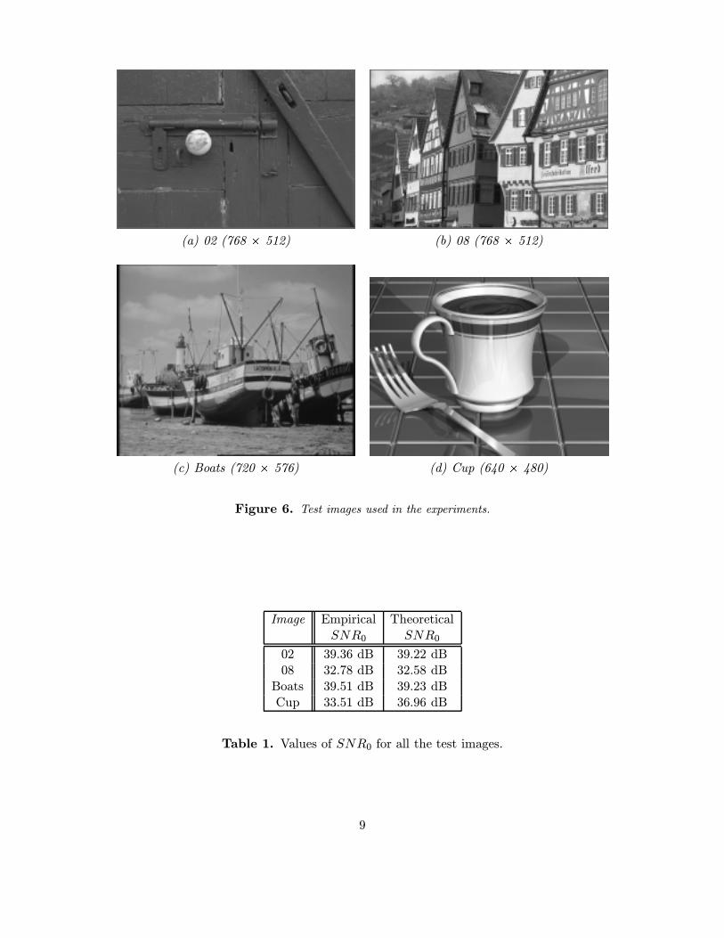
(a) 02 (768 � 512) (b) 08 (768 � 512)

(c) Boats (720 � 576) (d) Cup (640 � 480)

Figure 6. Test images used in the experiments.

Image Empirical TheoreticalSNR0 SNR0

02 39.36 dB 39.22 dB08 32.78 dB 32.58 dB

Boats 39.51 dB 39.23 dBCup 33.51 dB 36.96 dB

Table 1. Values of SNR0 for all the test images.

9

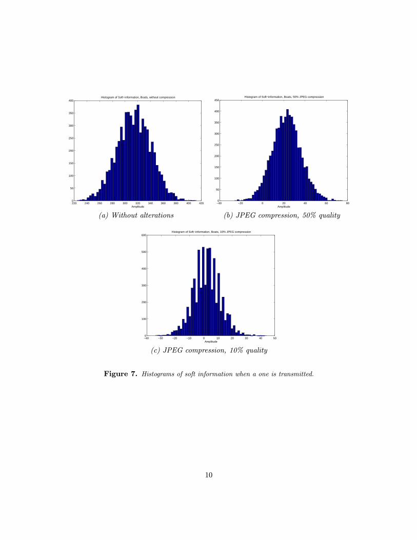
220 240 260 280 300 320 340 360 380 400 4200

50

100

150

200

250

300

350

400Histogram of Soft−information, Boats, without compression

Amplitude−40 −20 0 20 40 60 800

50

100

150

200

250

300

350

400

450Histogram of Soft−information, Boats, 50% JPEG compression

Amplitude

(a) Without alterations (b) JPEG compression, 50% quality

−40 −30 −20 −10 0 10 20 30 40 500

100

200

300

400

500

600Histogram of Soft−information, Boats, 10% JPEG compression

Amplitude

(c) JPEG compression, 10% quality

Figure 7. Histograms of soft information when a one is transmitted.

10

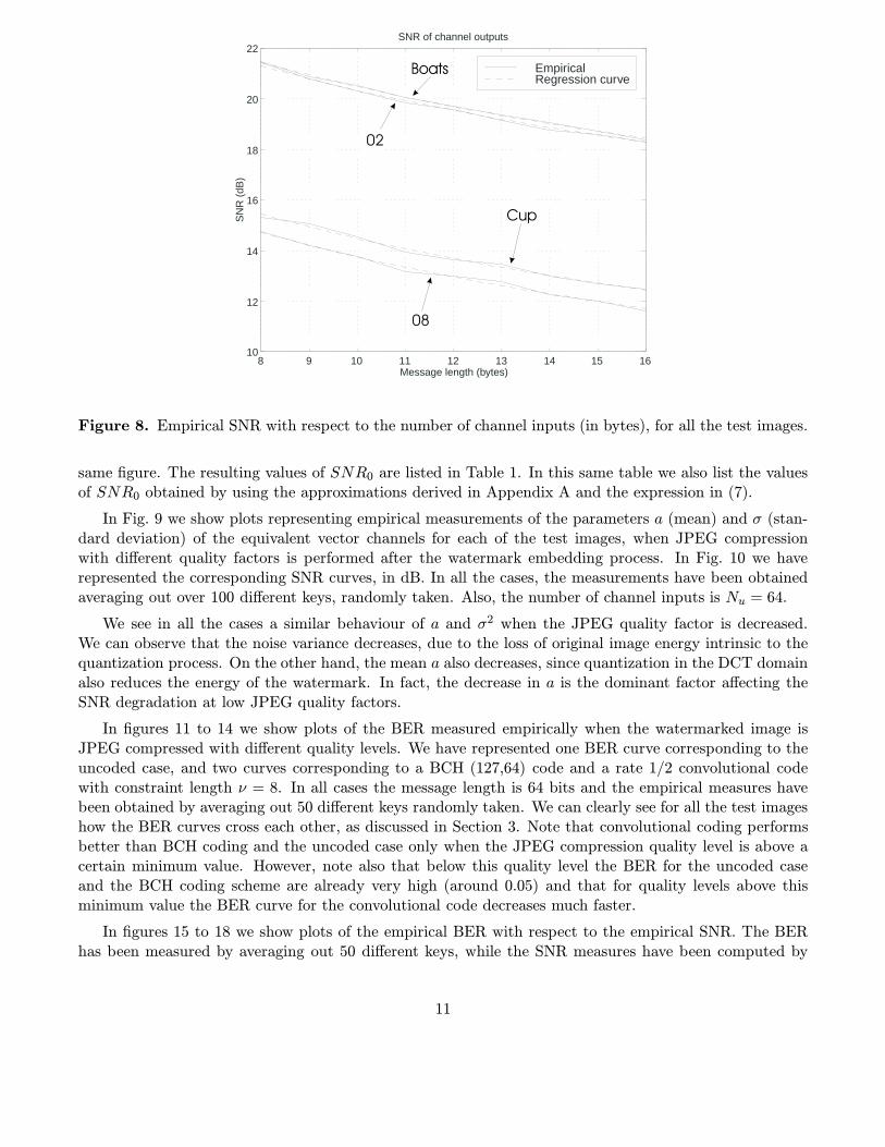
8 9 10 11 12 13 14 15 1610

12

14

16

18

20

22SNR of channel outputs

Message length (bytes)

SN

R(d

B)

EmpiricalRegression curve

Figure 8. Empirical SNR with respect to the number of channel inputs (in bytes), for all the test images.

same figure. The resulting values of SNR0 are listed in Table 1. In this same table we also list the valuesof SNR0 obtained by using the approximations derived in Appendix A and the expression in (7).

In Fig. 9 we show plots representing empirical measurements of the parameters a (mean) and σ (stan-dard deviation) of the equivalent vector channels for each of the test images, when JPEG compressionwith different quality factors is performed after the watermark embedding process. In Fig. 10 we haverepresented the corresponding SNR curves, in dB. In all the cases, the measurements have been obtainedaveraging out over 100 different keys, randomly taken. Also, the number of channel inputs is Nu = 64.

We see in all the cases a similar behaviour of a and σ2 when the JPEG quality factor is decreased.We can observe that the noise variance decreases, due to the loss of original image energy intrinsic to thequantization process. On the other hand, the mean a also decreases, since quantization in the DCT domainalso reduces the energy of the watermark. In fact, the decrease in a is the dominant factor affecting theSNR degradation at low JPEG quality factors.

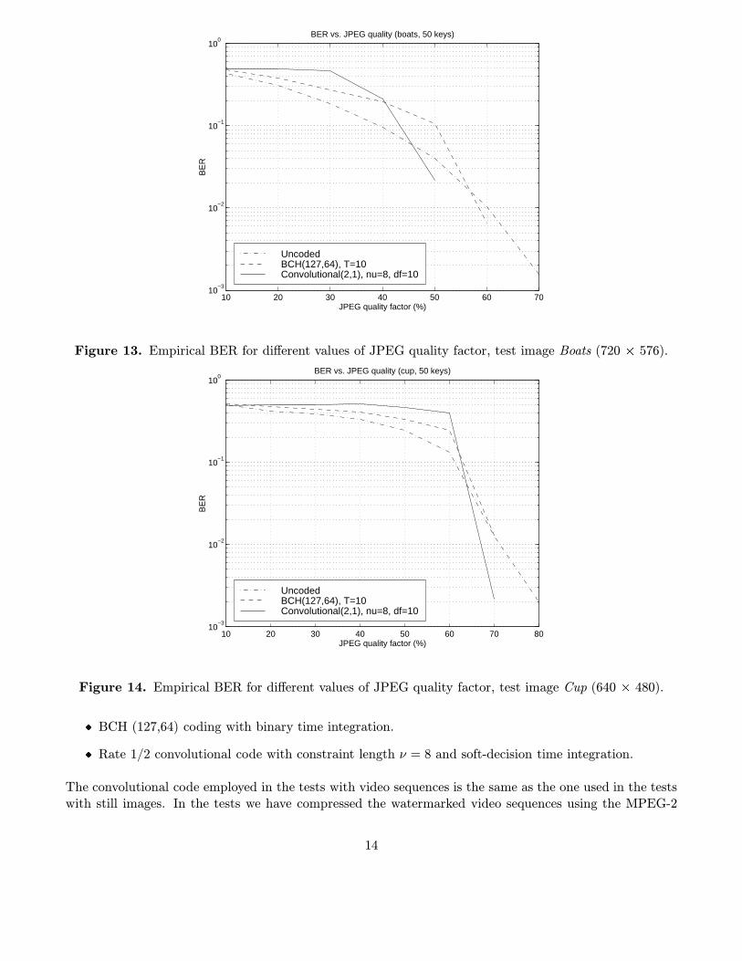
In figures 11 to 14 we show plots of the BER measured empirically when the watermarked image isJPEG compressed with different quality levels. We have represented one BER curve corresponding to theuncoded case, and two curves corresponding to a BCH (127,64) code and a rate 1/2 convolutional codewith constraint length ν = 8. In all cases the message length is 64 bits and the empirical measures havebeen obtained by averaging out 50 different keys randomly taken. We can clearly see for all the test imageshow the BER curves cross each other, as discussed in Section 3. Note that convolutional coding performsbetter than BCH coding and the uncoded case only when the JPEG compression quality level is above acertain minimum value. However, note also that below this quality level the BER for the uncoded caseand the BCH coding scheme are already very high (around 0.05) and that for quality levels above thisminimum value the BER curve for the convolutional code decreases much faster.

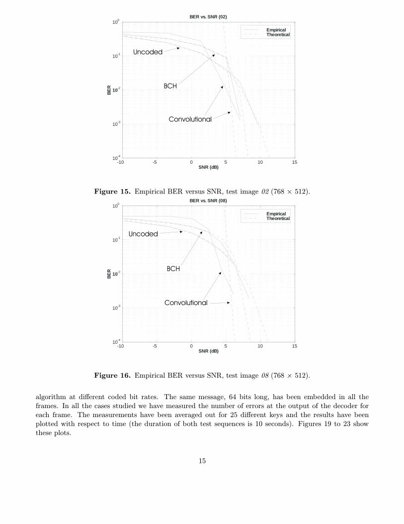
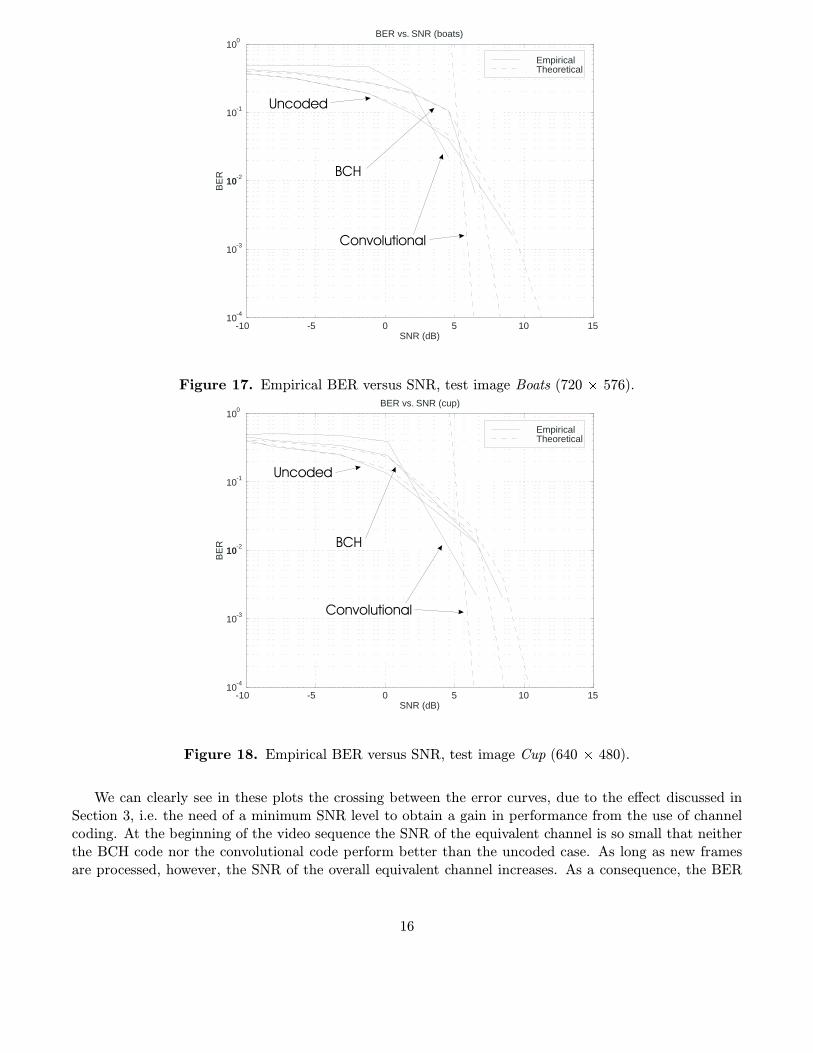
In figures 15 to 18 we show plots of the empirical BER with respect to the empirical SNR. The BERhas been measured by averaging out 50 different keys, while the SNR measures have been computed by

11

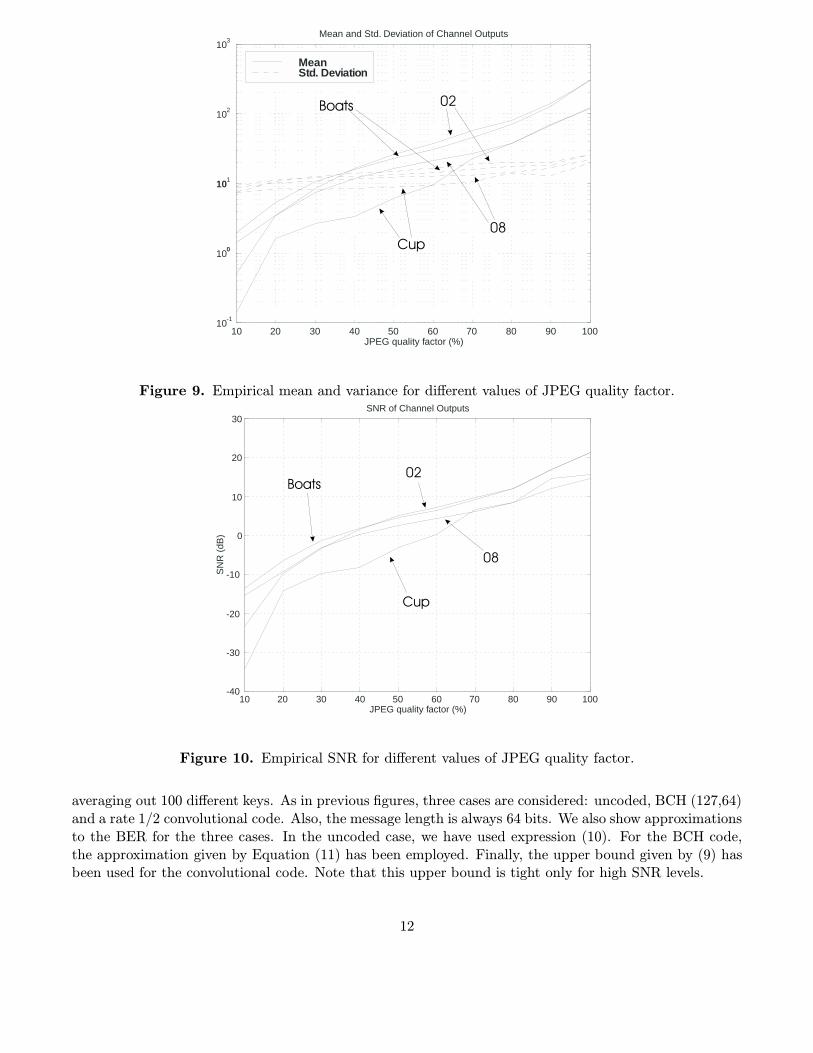
10 20 30 40 50 60 70 80 90 10010

-1

100

101

102

103

Mean and Std. Deviation of Channel Outputs

JPEG quality factor (%)

MeanStd. Deviation

Figure 9. Empirical mean and variance for different values of JPEG quality factor.

10 20 30 40 50 60 70 80 90 100-40

-30

-20

-10

0

10

20

30SNR of Channel Outputs

JPEG quality factor (%)

SN

R(d

B)

Figure 10. Empirical SNR for different values of JPEG quality factor.

averaging out 100 different keys. As in previous figures, three cases are considered: uncoded, BCH (127,64)and a rate 1/2 convolutional code. Also, the message length is always 64 bits. We also show approximationsto the BER for the three cases. In the uncoded case, we have used expression (10). For the BCH code,the approximation given by Equation (11) has been employed. Finally, the upper bound given by (9) hasbeen used for the convolutional code. Note that this upper bound is tight only for high SNR levels.

12

10 20 30 40 50 60 7010

−4

10−3

10−2

10−1

100

BER vs. JPEG quality (02, 50 keys)

JPEG quality factor (%)

BE

R

UncodedBCH(127,64), T=10Convolutional(2,1), nu=8, df=10

Figure 11. Empirical BER for different values of JPEG quality factor, test image 02 (768 � 512).

10 20 30 40 50 60 70 8010

−3

10−2

10−1

100

BER vs. JPEG quality (08, 50 keys)

JPEG quality factor (%)

BE

R

UncodedBCH(127,64), T=10Convolutional(2,1), nu=8, df=10

Figure 12. Empirical BER for different values of JPEG quality factor, test image 08 (768 � 512).

In order to assess the performance of the watermarking algorithms discussed in Section 4 for data hidingapplied to video sequences, we have performed tests with two video sequences (*** we should describe herecharacteristics of the video sequences. Maybe we should include one frame of each in the paper.***)employing three coding and decoding strategies:

� Uncoded, with binary time integration.

13

10 20 30 40 50 60 7010

−3

10−2

10−1

100

BER vs. JPEG quality (boats, 50 keys)

JPEG quality factor (%)

BE

R

UncodedBCH(127,64), T=10Convolutional(2,1), nu=8, df=10

Figure 13. Empirical BER for different values of JPEG quality factor, test image Boats (720 � 576).

10 20 30 40 50 60 70 8010

−3

10−2

10−1

100

BER vs. JPEG quality (cup, 50 keys)

JPEG quality factor (%)

BE

R

UncodedBCH(127,64), T=10Convolutional(2,1), nu=8, df=10

Figure 14. Empirical BER for different values of JPEG quality factor, test image Cup (640 � 480).

� BCH (127,64) coding with binary time integration.

� Rate 1/2 convolutional code with constraint length ν = 8 and soft-decision time integration.

The convolutional code employed in the tests with video sequences is the same as the one used in the testswith still images. In the tests we have compressed the watermarked video sequences using the MPEG-2

14

-10 -5 0 5 10 1510

-4

10-3

10-2

10-1

100

BER vs. SNR (02)

SNR (dB)

BE

R

EmpiricalTheoretical

Figure 15. Empirical BER versus SNR, test image 02 (768 � 512).

-10 -5 0 5 10 1510

-4

10-3

10-2

10-1

100

BER vs. SNR (08)

SNR (dB)

BE

R

EmpiricalTheoretical

Figure 16. Empirical BER versus SNR, test image 08 (768 � 512).

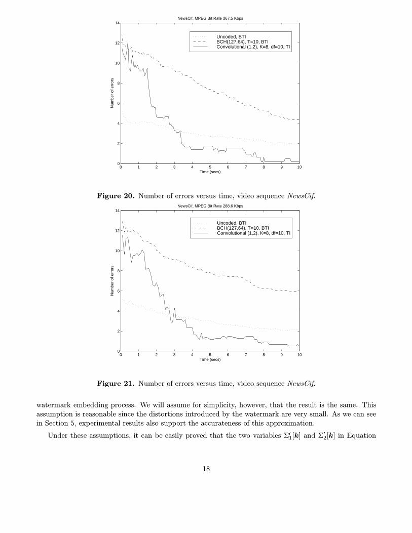
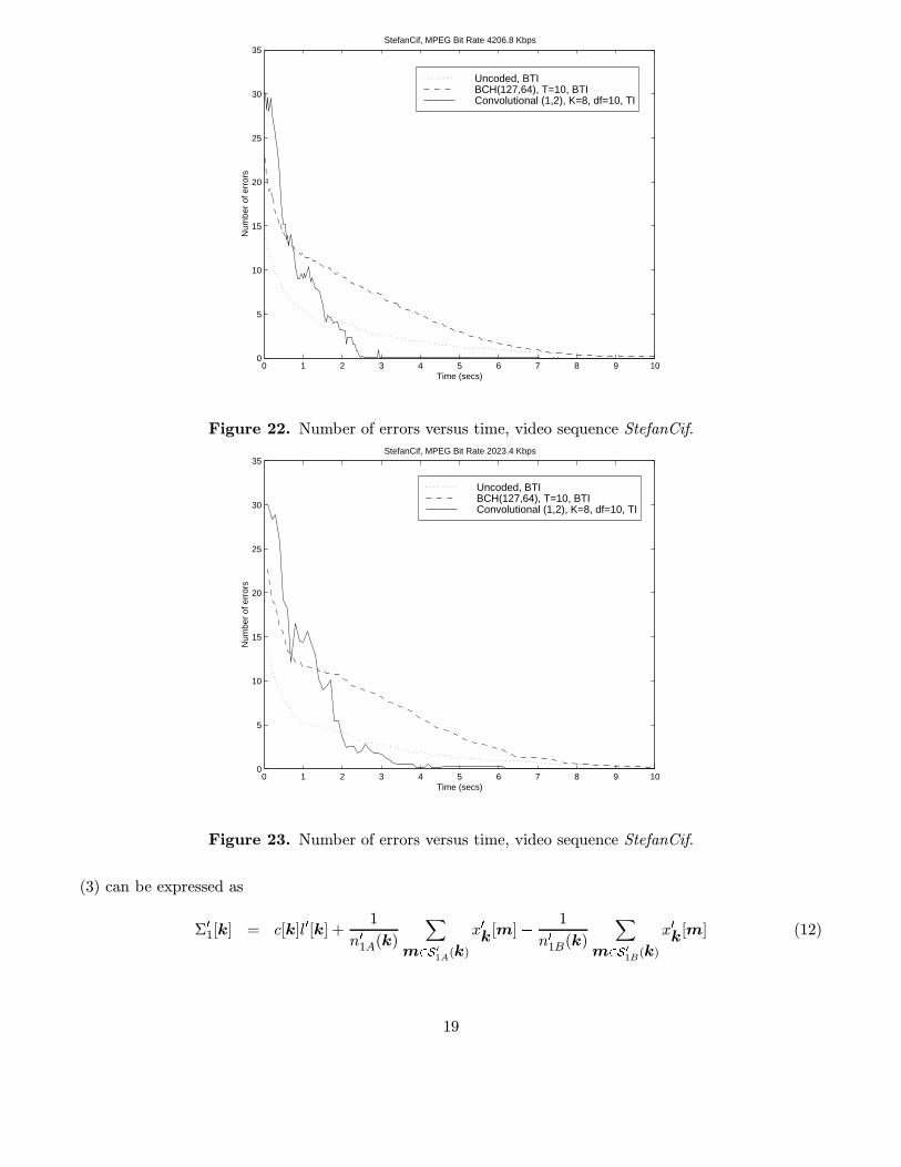
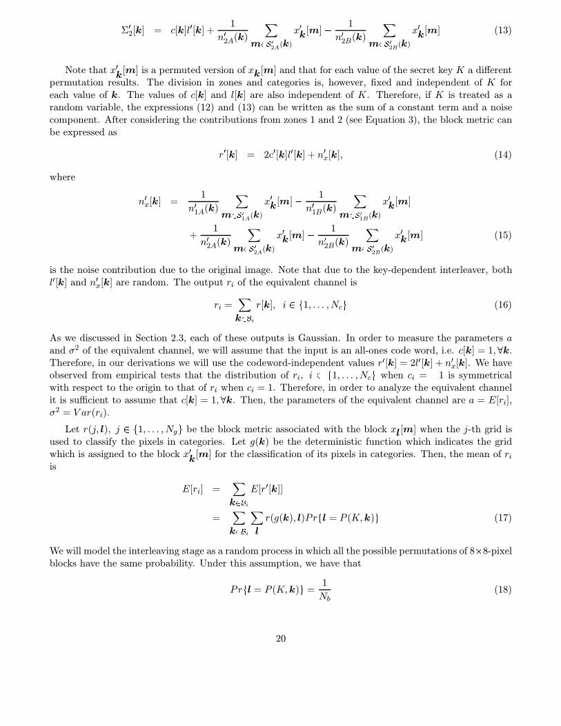
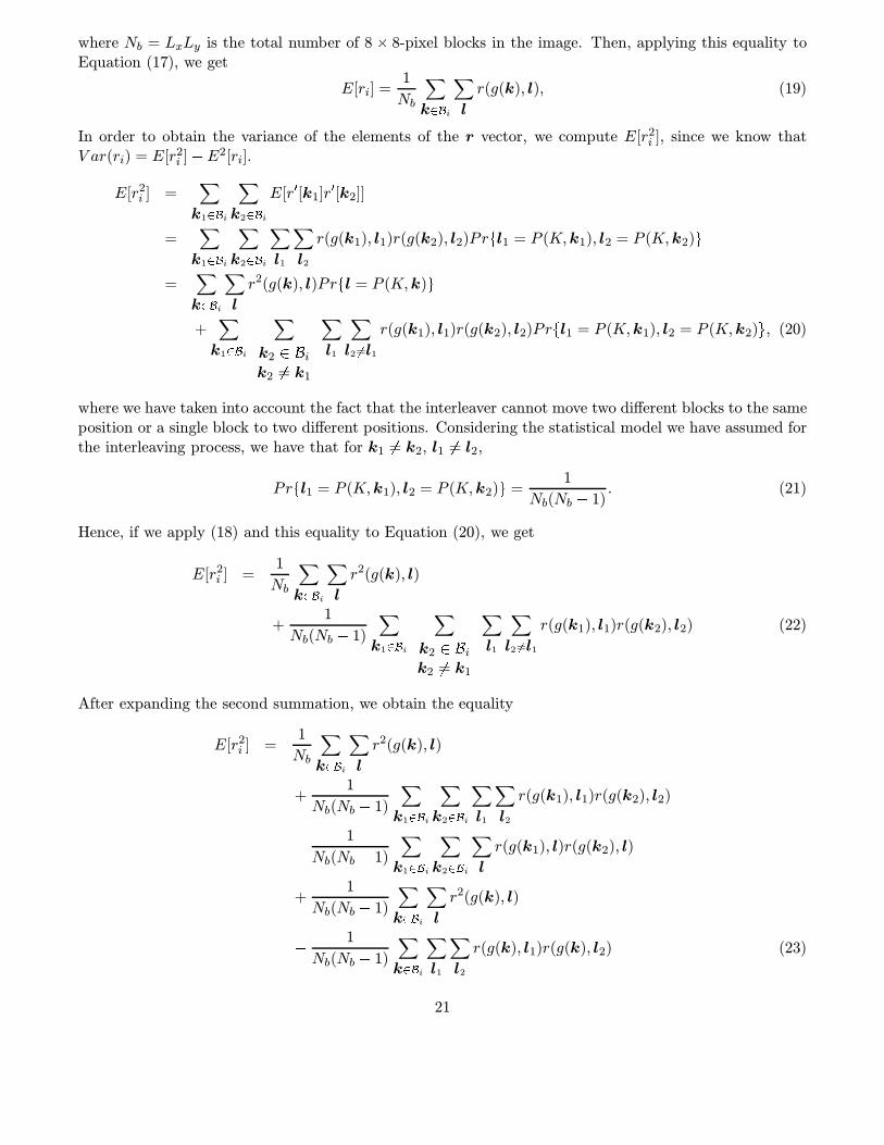
algorithm at different coded bit rates. The same message, 64 bits long, has been embedded in all theframes. In all the cases studied we have measured the number of errors at the output of the decoder foreach frame. The measurements have been averaged out for 25 different keys and the results have beenplotted with respect to time (the duration of both test sequences is 10 seconds). Figures 19 to 23 showthese plots.

15

-10 -5 0 5 10 1510

-4

10-3

10-2

10-1

100

BER vs. SNR (boats)

SNR (dB)

BE

R

EmpiricalTheoretical

Figure 17. Empirical BER versus SNR, test image Boats (720 � 576).

-10 -5 0 5 10 1510

-4

10-3

10-2

10-1

100

BER vs. SNR (cup)

SNR (dB)

BE

R

EmpiricalTheoretical

Figure 18. Empirical BER versus SNR, test image Cup (640 � 480).

We can clearly see in these plots the crossing between the error curves, due to the effect discussed inSection 3, i.e. the need of a minimum SNR level to obtain a gain in performance from the use of channelcoding. At the beginning of the video sequence the SNR of the equivalent channel is so small that neitherthe BCH code nor the convolutional code perform better than the uncoded case. As long as new framesare processed, however, the SNR of the overall equivalent channel increases. As a consequence, the BER

16

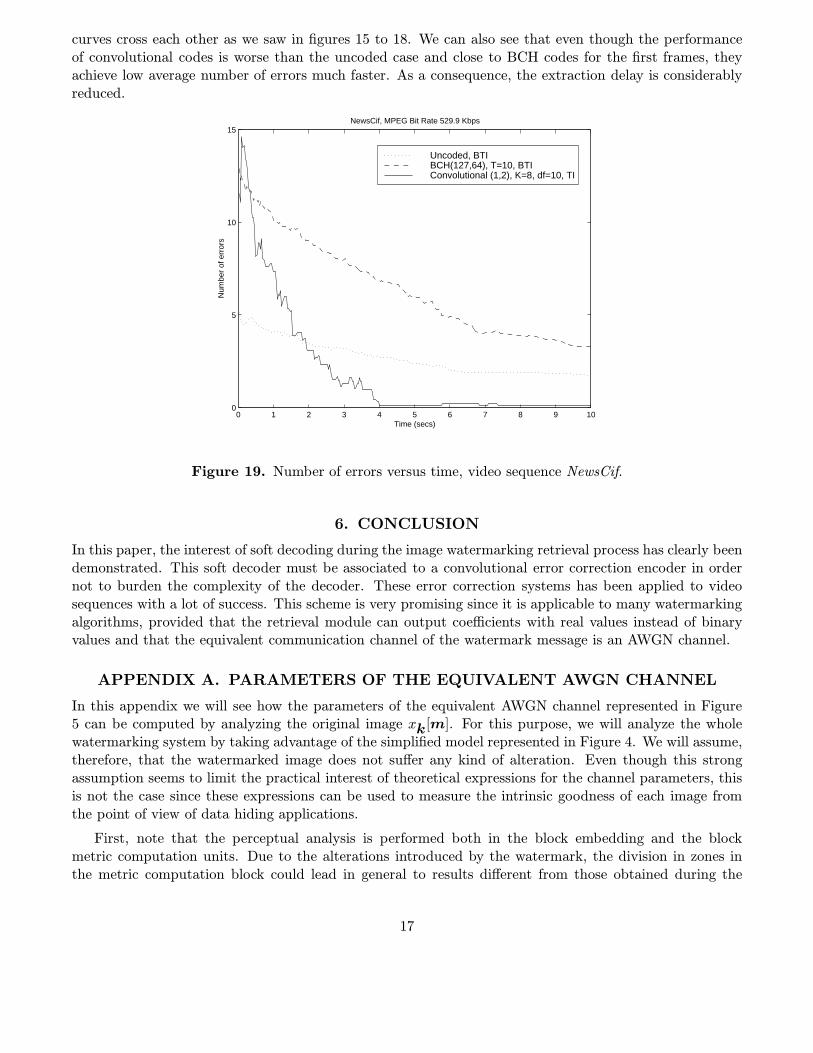
curves cross each other as we saw in figures 15 to 18. We can also see that even though the performanceof convolutional codes is worse than the uncoded case and close to BCH codes for the first frames, theyachieve low average number of errors much faster. As a consequence, the extraction delay is considerablyreduced.

0 1 2 3 4 5 6 7 8 9 100

5

10

15NewsCif, MPEG Bit Rate 529.9 Kbps

Time (secs)

Num

ber

of e

rror

s

Uncoded, BTIBCH(127,64), T=10, BTIConvolutional (1,2), K=8, df=10, TI

Figure 19. Number of errors versus time, video sequence NewsCif.

6. CONCLUSION

In this paper, the interest of soft decoding during the image watermarking retrieval process has clearly beendemonstrated. This soft decoder must be associated to a convolutional error correction encoder in ordernot to burden the complexity of the decoder. These error correction systems has been applied to videosequences with a lot of success. This scheme is very promising since it is applicable to many watermarkingalgorithms, provided that the retrieval module can output coefficients with real values instead of binaryvalues and that the equivalent communication channel of the watermark message is an AWGN channel.

APPENDIX A. PARAMETERS OF THE EQUIVALENT AWGN CHANNEL

In this appendix we will see how the parameters of the equivalent AWGN channel represented in Figure5 can be computed by analyzing the original image xk[m]. For this purpose, we will analyze the wholewatermarking system by taking advantage of the simplified model represented in Figure 4. We will assume,therefore, that the watermarked image does not suffer any kind of alteration. Even though this strongassumption seems to limit the practical interest of theoretical expressions for the channel parameters, thisis not the case since these expressions can be used to measure the intrinsic goodness of each image fromthe point of view of data hiding applications.

First, note that the perceptual analysis is performed both in the block embedding and the blockmetric computation units. Due to the alterations introduced by the watermark, the division in zones inthe metric computation block could lead in general to results different from those obtained during the

17

0 1 2 3 4 5 6 7 8 9 100

2

4

6

8

10

12

14NewsCif, MPEG Bit Rate 367.5 Kbps

Time (secs)

Num

ber

of e

rror

s

Uncoded, BTIBCH(127,64), T=10, BTIConvolutional (1,2), K=8, df=10, TI

Figure 20. Number of errors versus time, video sequence NewsCif.

0 1 2 3 4 5 6 7 8 9 100

2

4

6

8

10

12

14NewsCif, MPEG Bit Rate 288.6 Kbps

Time (secs)

Num

ber

of e

rror

s

Uncoded, BTIBCH(127,64), T=10, BTIConvolutional (1,2), K=8, df=10, TI

Figure 21. Number of errors versus time, video sequence NewsCif.

watermark embedding process. We will assume for simplicity, however, that the result is the same. Thisassumption is reasonable since the distortions introduced by the watermark are very small. As we can seein Section 5, experimental results also support the accurateness of this approximation.

Under these assumptions, it can be easily proved that the two variables Σ01[k] and Σ0

2[k] in Equation

18

0 1 2 3 4 5 6 7 8 9 100

5

10

15

20

25

30

35StefanCif, MPEG Bit Rate 4206.8 Kbps

Time (secs)

Num

ber

of e

rror

s

Uncoded, BTIBCH(127,64), T=10, BTIConvolutional (1,2), K=8, df=10, TI

Figure 22. Number of errors versus time, video sequence StefanCif.

0 1 2 3 4 5 6 7 8 9 100

5

10

15

20

25

30

35StefanCif, MPEG Bit Rate 2023.4 Kbps

Time (secs)

Num

ber

of e

rror

s

Uncoded, BTIBCH(127,64), T=10, BTIConvolutional (1,2), K=8, df=10, TI

Figure 23. Number of errors versus time, video sequence StefanCif.

(3) can be expressed as

Σ01[k] = c[k]l0[k] +

1

n01A(k)

∑m2S01A(k)

x0k[m]� 1

n01B(k)

∑m2S01B(k)

x0k[m] (12)

19

Σ02[k] = c[k]l0[k] +

1

n02A(k)

∑m2S02A(k)

x0k[m]� 1

n02B(k)

∑m2S02B(k)

x0k[m] (13)

Note that x0k[m] is a permuted version of xk[m] and that for each value of the secret key K a differentpermutation results. The division in zones and categories is, however, fixed and independent of K foreach value of k. The values of c[k] and l[k] are also independent of K. Therefore, if K is treated as arandom variable, the expressions (12) and (13) can be written as the sum of a constant term and a noisecomponent. After considering the contributions from zones 1 and 2 (see Equation 3), the block metric canbe expressed as

r0[k] = 2c0[k]l0[k] + n0x[k], (14)

where

n0x[k] =1

n01A(k)

∑m2S01A(k)

x0k[m]� 1

n01B(k)

∑m2S01B(k)

x0k[m]

+1

n02A(k)

∑m2S0

2A(k)

x0k[m]� 1

n02B(k)

∑m2S0

2B(k)

x0k[m] (15)

is the noise contribution due to the original image. Note that due to the key-dependent interleaver, bothl0[k] and n0x[k] are random. The output ri of the equivalent channel is

ri =∑k2Bi

r[k], i 2 f1, . . . ,Ncg (16)

As we discussed in Section 2.3, each of these outputs is Gaussian. In order to measure the parameters aand σ2 of the equivalent channel, we will assume that the input is an all-ones code word, i.e. c[k] = 1,8k.Therefore, in our derivations we will use the codeword-independent values r0[k] = 2l0[k] + n0x[k]. We haveobserved from empirical tests that the distribution of ri, i 2 f1, . . . ,Ncg when ci = �1 is symmetricalwith respect to the origin to that of ri when ci = 1. Therefore, in order to analyze the equivalent channelit is sufficient to assume that c[k] = 1,8k. Then, the parameters of the equivalent channel are a = E[ri],σ2 = V ar(ri).

Let r(j, l), j 2 f1, . . . ,Ngg be the block metric associated with the block xl[m] when the j-th grid isused to classify the pixels in categories. Let g(k) be the deterministic function which indicates the gridwhich is assigned to the block x0k[m] for the classification of its pixels in categories. Then, the mean of riis

E[ri] =∑k2Bi

E[r0[k]]

=∑k2Bi

∑l

r(g(k), l)Prfl = P (K,k)g (17)

We will model the interleaving stage as a random process in which all the possible permutations of 8�8-pixelblocks have the same probability. Under this assumption, we have that

Prfl = P (K,k)g = 1

Nb(18)

20

where Nb = LxLy is the total number of 8 � 8-pixel blocks in the image. Then, applying this equality toEquation (17), we get

E[ri] =1

Nb

∑k2Bi

∑l

r(g(k), l), (19)

In order to obtain the variance of the elements of the r vector, we compute E[r2i ], since we know thatV ar(ri) = E[r

2i ]�E2[ri].

E[r2i ] =∑k12Bi

∑k22Bi

E[r0[k1]r0[k2]]

=∑k12Bi

∑k22Bi

∑l1

∑l2

r(g(k1), l1)r(g(k2), l2)Prfl1 = P (K,k1), l2 = P (K,k2)g

=∑k2Bi

∑l

r2(g(k), l)Prfl = P (K,k)g

+∑k12Bi

∑k2 2 Bik2 6= k1

∑l1

∑l2 6=l1

r(g(k1), l1)r(g(k2), l2)Prfl1 = P (K,k1), l2 = P (K,k2)g, (20)

where we have taken into account the fact that the interleaver cannot move two different blocks to the sameposition or a single block to two different positions. Considering the statistical model we have assumed forthe interleaving process, we have that for k1 6= k2, l1 6= l2,

Prfl1 = P (K,k1), l2 = P (K,k2)g =1

Nb(Nb � 1). (21)

Hence, if we apply (18) and this equality to Equation (20), we get

E[r2i ] =1

Nb

∑k2Bi

∑l

r2(g(k), l)

+1

Nb(Nb � 1)

∑k12Bi

∑k2 2 Bik2 6= k1

∑l1

∑l2 6=l1

r(g(k1), l1)r(g(k2), l2) (22)

After expanding the second summation, we obtain the equality

E[r2i ] =1

Nb

∑k2Bi

∑l

r2(g(k), l)

+1

Nb(Nb � 1)

∑k12Bi

∑k22Bi

∑l1

∑l2

r(g(k1), l1)r(g(k2), l2)

� 1

Nb(Nb � 1)

∑k12Bi

∑k22Bi

∑l

r(g(k1), l)r(g(k2), l)

+1

Nb(Nb � 1)

∑k2Bi

∑l

r2(g(k), l)

� 1

Nb(Nb � 1)

∑k2Bi

∑l1

∑l2

r(g(k), l1)r(g(k), l2) (23)

21

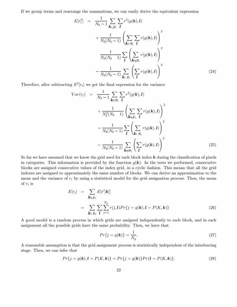
If we group terms and rearrange the summations, we can easily derive the equivalent expression

E[r2i ] =1

Nb � 1

∑k2Bi

∑l

r2(g(k), l)

+1

Nb(Nb � 1)

∑k2Bi

∑l

r(g(k), l)

2

� 1

Nb(Nb � 1)

∑l

∑k2Bi

r(g(k), l)

2

� 1

Nb(Nb � 1)

∑k2Bi

∑l

r(g(k), l)

2

(24)

Therefore, after subtracting E2[ri] we get the final expression for the variance

V ar(ri) =1

Nb � 1

∑k2Bi

∑l

r2(g(k), l)

+1

N2b (Nb � 1)

∑k2Bi

∑l

r(g(k), l)

2

� 1

Nb(Nb � 1)

∑l

∑k2Bi

r(g(k), l)

2

� 1

Nb(Nb � 1)

∑k2Bi

∑l

r(g(k), l)

2

(25)

So far we have assumed that we know the grid used for each block index k during the classification of pixelsin categories. This information is provided by the function g(k). In the tests we performed, consecutiveblocks are assigned consecutive values of the index grid, in a cyclic fashion. This means that all the gridindexes are assigned to approximately the same number of blocks. We can derive an approximation to themean and the variance of ri by using a statistical model for the grid assignation process. Then, the meanof ri is

E[ri] =∑k2Bi

E[r0[k]]

=∑k2Bi

∑l

Ng∑j=1

r(j, l)Prfj = g(k), l = P (K,k)g (26)

A good model is a random process in which grids are assigned independently to each block, and in eachassignment all the possible grids have the same probability. Then, we have that

Prfj = g(k)g = 1

Ng. (27)

A reasonable assumption is that the grid assignment process is statistically independent of the interleavingstage. Then, we can infer that

Prfj = g(k), l = P (K,k)g = Prfj = g(k)gPrfl = P (K,k)g. (28)

22

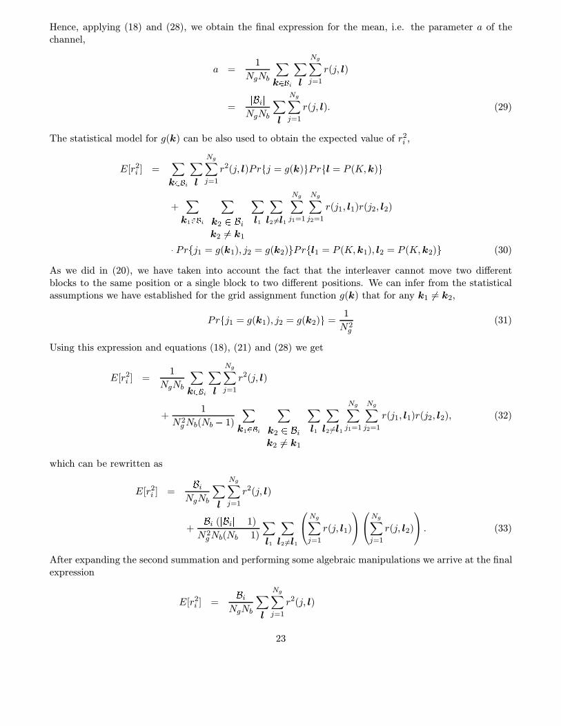
Hence, applying (18) and (28), we obtain the final expression for the mean, i.e. the parameter a of thechannel,

a =1

NgNb

∑k2Bi

∑l

Ng∑j=1

r(j, l)

=jBijNgNb

∑l

Ng∑j=1

r(j, l). (29)

The statistical model for g(k) can be also used to obtain the expected value of r2i ,

E[r2i ] =∑k2Bi

∑l

Ng∑j=1

r2(j, l)Prfj = g(k)gPrfl = P (K,k)g

+∑k12Bi

∑k2 2 Bik2 6= k1

∑l1

∑l2 6=l1

Ng∑j1=1

Ng∑j2=1

r(j1, l1)r(j2, l2)

� Prfj1 = g(k1), j2 = g(k2)gPrfl1 = P (K,k1), l2 = P (K,k2)g (30)

As we did in (20), we have taken into account the fact that the interleaver cannot move two differentblocks to the same position or a single block to two different positions. We can infer from the statisticalassumptions we have established for the grid assignment function g(k) that for any k1 6= k2,

Prfj1 = g(k1), j2 = g(k2)g =1

N2g(31)

Using this expression and equations (18), (21) and (28) we get

E[r2i ] =1

NgNb

∑k2Bi

∑l

Ng∑j=1

r2(j, l)

+1

N2gNb(Nb � 1)

∑k12Bi

∑k2 2 Bik2 6= k1

∑l1

∑l2 6=l1

Ng∑j1=1

Ng∑j2=1

r(j1, l1)r(j2, l2), (32)

which can be rewritten as

E[r2i ] =jBijNgNb

∑l

Ng∑j=1

r2(j, l)

+jBij(jBij � 1)

N2gNb(Nb � 1)

∑l1

∑l2 6=l1

Ng∑j=1

r(j, l1)

Ng∑j=1

r(j, l2)

. (33)

After expanding the second summation and performing some algebraic manipulations we arrive at the finalexpression

E[r2i ] =jBijNgNb

∑l

Ng∑j=1

r2(j, l)

23

+jBij(jBij � 1)

N2gNb(Nb � 1)

∑l

Ng∑j=1

r(j, l)

2

� jBij(jBij � 1)

N2gNb(Nb � 1)

∑l

Ng∑j=1

r(j, l)

2

(34)

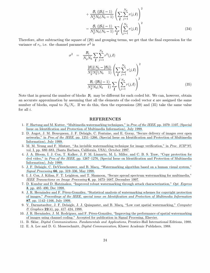
Therefore, after subtracting the square of (29) and grouping terms, we get that the final expression for thevariance of ri, i.e. the channel parameter σ2 is

σ2 =jBijNgNb

∑l

Ng∑j=1

r2(j, l)

� jBij(Nb � jBij)N2gN

2b (Nb � 1)

∑l

Ng∑j=1

r(j, l)

2

� jBij(jBij � 1)

N2gNb(Nb � 1)

∑l

Ng∑j=1

r(j, l)

2

(35)

Note that in general the number of blocks jBij may be different for each coded bit. We can, however, obtainan accurate approximation by assuming that all the elements of the coded vector c are assigned the samenumber of blocks, equal to Nb/Nc. If we do this, then the expressions (29) and (35) take the same valuefor all i.

REFERENCES

1. F. Hartung and M. Kutter, “Multimedia watermarking techniques,” in Proc.of the IEEE, pp. 1079–1107, (SpecialIssue on Identification and Protection of Multimedia Information), July 1999.

2. D. Augot, J. M. Boucqueau, J. F. Delaigle, C. Fontaine, and E. Goray, “Secure delivery of images over opennetworks,” in Proc.of the IEEE, pp. 1251–1266, (Special Issue on Identification and Protection of MultimediaInformation), July 1999.

3. M. M. Yeung and F. Mintzer, “An invisible watermarking technique for image verification,” in Proc. ICIP’97,vol. I, pp. 680–683, (Santa Barbara, California, USA), October 1997.

4. J. A. Bloom, I. J. Cox, T. Kalker, J. P. M. Linnartz, M. L. Miller, and C. B. S. Traw, “Copy protection fordvd video,” in Proc.of the IEEE, pp. 1267–1276, (Special Issue on Identification and Protection of MultimediaInformation), July 1999.

5. J. F. Delaigle, C. DeVleeschouwer, and B. Macq, “Watermarking algorithm based on a human visual system,”Signal Processing 66, pp. 319–336, May 1998.

6. I. J. Cox, J. Kilian, F. T. Leighton, and T. Shamoon, “Secure spread spectrum watermarking for multimedia,”IEEE Transactions on Image Processing 6, pp. 1673–1687, December 1997.

7. D. Kundur and D. Hatzinakos, “Improved robust watermarking through attack characterization,” Opt. Express3, pp. 485–490, Dec 1998.

8. J. R. Hernandez and F. Perez-Gonzalez, “Statistical analysis of watermarking schemes for copyright protectionof images,” Proceedings of the IEEE, special issue on Identification and Protection of Multimedia Information87, pp. 1142–1166, July 1999.

9. V. Darmstaedter, J. F. Delaigle, J. J. Quisquater, and B. Macq, “Low cost spatial watermarking,” Computer& Graphics 22(4), pp. 417–424, 1998.

10. J. R. Hernandez, J. M. Rodrıguez, and F. Perez-Gonzalez, “Improving the performance of spatial watermarkingof images using channel coding.” Accepted for publication in Signal Procesing, Elsevier.

11. B. Sklar, Digital Communications. Fundamentals and Applications, Prentice-Hall International Editions, 1988.

12. E. A. Lee and D. G. Messerschmitt, Digital Communication, Kluwer Academic Publishers, 1988.

24