PRODUCTIVITY DECODING OF FINANCIAL SIGNALS
149
PRODUCTIVITY DECODING OF FINANCIAL SIGNALS: A PRIMER FOR MANAGERS ON DETERMINISTIC PRODUCTIVITY ACCOUNfiNG V The Library BAZILJ. VAN of tlic Witwaterstand Johannesburg by WtTMEA PUBLISHER Productivity Measurement Associates United Kingdom
-
Upload
fami4real2000 -
Category
Documents
-
view
0 -
download
0
Transcript of PRODUCTIVITY DECODING OF FINANCIAL SIGNALS
PRODUCTIVITY DECODING OFFINANCIAL SIGNALS:
A PRIMER FOR MANAGERS ONDETERMINISTIC PRODUCTIVITY ACCOUNfiNG
V
The Library BAZILJ. VAN
of tlic Witwaterstand
Johannesburg
by
WtTMEA
PUBLISHERProductivity Measurement AssociatesUnited Kingdom
This book is copyright under the Berne Convention. In termsof the Copyright Act, No 98 of 1978, no part of this book maybe reproduced or transmitted in any form or by any means,electronic or mechanical, including photocopying, recording orby information storage and retrieval system, without permissionin writing from the Publisher.
Key words:- ProductivityDecodeFinancialSignalsManagerDeterministicAccounting
Prior to publication of this book, I communicated the ofdeterministic productivity accounting to university students and tothrough lectures, articles and books which assume the reader hat anappreciation of advanced mathematics.
This book attempts to introduce another dimension to the literature thesubject. It aims at providing the non—mathematical reader an overview q theproductivity notion and relates.the "hard" (i.e., mathematicallynotion of productivity measurement to the "soft" objective of
in a manner conducive to raising productivity.
My principal business activity is training and providing consulting sqtjportto management of corporations who have decided to adoptproductivity accounting as part of the productivity management jqtjrneydescribed jn this book. In addition, I enjoy lecturing part—time inuniversities on the subject covered by this book to both andpostgraduate students in engineering and commerce faculties. Such teictingactivities revealed a need for an introductory text book which providflt anoverview of the productivity concept and the role of productivityin improving productivity.
The demand for such a book extends beyond universities into the pqlicyformation arena as governments increasingly acknowledge the need for contreteprograms to foster productivity growth. Government agencies theriforeacknowledge that they are also targets for the ideas expressed in this
To simplify the measurement component of the ideas set forth in this asimple notation is employed. A more quantitative audience is referred myother works for a rigurous algebraic specification of the axioms on thework rests.
Growing awareness of this work in academic circles is evident from theincreasing number of candidates for higher degrees who aspire to use this &jorkfor their research. It is interesting that some candidates intendthe mathematical structure while others intend taking it as given to moflitorprogress in the soft i:omponents of the productivity improvement process.
Growing awareness of this work in business circles flows from two roots, Itis stimulated in part by a management recognition thatimprovement is a good idea whose time has come. It is also stimulated injartby the activities of postgraduate university students who perceive the peedfor sound productivity measurement to underpin systematic efforts tooperations and raise productivity.
I hope that this bcok will therefore serve the needs of productivityconstituents in universities, business and government. Toupfront intellectual investment which users of the concept need to make, barehas been taken to include an expert system in the latest softwareknown as Financial Productivity Management (FPM). Hence the principal Ueascontained in this book can readily be accessed from the software inform to reinforce in the mind of the user what is stated more fullybook.
Bazil J. van.
To the Players, onsite and offsite
COPYRIGHT 1988 Basil James van Loggerenberg
PREFACE
"In their deep concerns men clever enough to dissimulate". C.P. Snow
Published by
Productivity Measurement AssociatesP.O. Box 201WITS 2050
301014429
ISBN 0 620 10540 2BDOZZO61
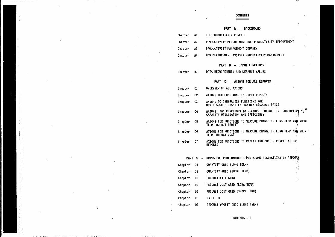
CONTENTS
PART A — BACKGROUND
Chapter Al TIlE PRODUCTIVITY CONCEPT
Chapter AZ PRODUCTIVITY MEASUREMENT AND PRODUCTIVITY IMPROVEMENT
Chapter A3 PRODUCTIVITY MANAGEMENT JOURNEY
Chapter A4 HOW MEASUREMENT ASSISTS PRODUCTIVITY MANAGEMENT
PART B — INPUT FUNCTIONS
Chapter Bl DATA REQUIREMENTS AND DEFAULT VALUES
PART C — AXIOMS FOR ALL REPORTS
Chapter Cl OVERVIEW OF ALL AXIOMS
Chapter C2 AXIOMS FOR FUNCTIONS IN INPUT REPORTS
Chapter C3 AXIOMS TO GENERALIZE FUNCTIONS FORNEW RESOURCE QUANTITY AND NEW RESOURCE PRICE
Chapter C4 AXIOMS FOR FUNCTIONS TO MEASURE CHANGE IN PRODUCTIVITY,4CAPACITY UTILIZATION AND EFFICIENCY
Chapter C5 AXIOMS FOR FUNCTIONS TO MEASURE CHANGE IN LONG TERM SHORT
TERM PRODUCT PROFIT
Chapter C6 AXIOMS FOR FUNCTIONS TO MEASURE CHANGE IN LONG TERM ANQ SHORTTERM PRODUCT COST
Chapter C7 AXIOMS FOR FUNCTIONS IN PROFIT AND COST RECONCILIATIONRE PORTS
PART 0 — GRIDS FOR PERFORMANCE REPORTS AND RECONCILIATION
Chapter Dl QUANTITY GRID (LONG TERM)
Chapter D2 QUANTITY GRID (SHORT TERM)
Chapter D3 PRODUCTIVITY GRID
Chapter D4 PRODUCT COST GRID (LONG TERM)
Chapter D5 PRODUCT COST GRID (SHORT TERM)
Chapter D6 PRiCE GRID
Chapter 07 PRODUCT PROFIT GRID (LONG TERM)
CONTENTS — I
Chapter
Chapter
Chapter
Chapter
Chapter
Chapter
Chapter
D8
09
D10
011
012
D13
Dl 4
CONTENTS — 2
Chapter 12 DETERMINISTIC PRODUCTIVITY ACCOUNTING EXTENSIONTO BENEFIT TO COST RATIOS
APPENDIX B - BIBLIOGRAPHY
CONTENTS — 3
PRODUCT PROFIT GRID (SHORT TERM)
PRODUCT MIX COST GRID
PRODUCT VOLUME COST GRID
INVESTMENT VARIANCE PROFIT GRID
RETURN ON REVENUE VARIANCE PROFIT GRID
TARGET ROI PROFIT GRID
GRIDS RECOMMENDED FOR PRODUCTIVITY DISCLOSURE
PART F — RESOURCE VARIABILITY (REVA
Chapter Fl 'VARIOUS CASES OF REVA
PART G — PROXY DATA
Chapter Gl PROXY PRICES AND PROXY QUANTITIES WHEN NONE ARE AVAILAWI
Chapter G2 SCORING MATRICES FOR PROXY PRODUCT QUANTITY
PART H — TRADEOFF ANALYSIS
Chapter Hl TRADITIONAL PRODUCTIVITY INDEX NUMBERS AND WORK STUDYAPPROACHES
Chapter HZ TRADITIONAL INFLATION ACCOUNTING APPROACH
Chapter H3 1RADITIONAL STANDARD COST ACCOUNTING APPROACH ANDEXPENSE TO REVENUE RATIO APPROACH
Chapter H4 DETERMINISTIC PRODUCTIVITY ACCOUNTING APPROACH
Chapter H5 COMPARISON OF TRADITIONAL STANDARD COSTING ANDPRODUCTIVITY ACCOUNTING APPROACHES
PART I — NET PRESENT VALUE
Chapter Ii DETERMINISTIC PRODUCTIVITY ACCOUNTING EXTENSIONTC NET PRESENT VALUE ANALYSIS
PART E — EXAMPLE
Chapter El EXAMPLE OF INPUT VALIDATION "A" REPORT
Chapter E2 EXAMPLE OF INPUT VALIDATION "B" REPORT
Chapter E3 EXAMPLE OF INPUT VARIANCE REPORT
Chapter E4 EXAMPLE OF INPUT RELATIVE REPORT
Chapter ES EXAMPLE OF INPUT COMPACT REPORT
Chapter E6 EXAMPLE OF INPUT NORMALIZED QUANTITY AND PRICE REPORT
Chapter E7 EXAMPLE OF PROFIT BACKGROUND REPORT
Chapter E8 EXAMPLE OF PROFIT RECONCILIATION REPORT
Chapter E9 EXAMPLE OF PROFIT OVERVIEW REPORT
Chapter E1O EXAMPLE OF LONG TERM PRODUCT PROFIT REPORT
Chapter Eli EXAMPLE OF SHORT TERM PROOUCT PROFIT REPORT
Chapter E12 EXAMPLE OF COST RECONCILIATION REPORT
Chapter E13 EXAMPLE OF COST OVERVIEW REPORT
Chapter
Chapter
EI4
ElS
EXAMPLE OF LONG TERM PRODUCT COST REPORT
EXAMPLE OF SHORT TERM PRODUCT COST REPORT
Chapter E16 EXAMPLE OF PRODUCTIVITY OLD AND NEW VARIANCE REPORT
Chapter E17 EXAMPLE OF PRODUCTIVITY COMPONENT VARIANCE REPORT
Chapter E18 EXAMPLE OF PRODUCTIVITY COMPONENT OLD & NEW REPORT
PART ,J — UNIT LIFE CYCLE COST
Chapter JI DETERMINISTIC PRODUCTIVITY ACCOUNTING EXTENSIONTO UNIT LIFE CYCLE COST ANALYSIS
PART K — PRODUCT NORMALIZATIONS
Chapter KI AXIOMS TO NORMALIZE NEW LEVELS OF PRODUCT QUANTITY AND PftICE
APPENDIX A - SPECIMEN EXPERT SYSTEM REPORTS
I
PART A — BACKGROUND
This part of the book presents the following 4 chapters.
Chapter Al THE PRODUCTIVITY CONCEPT
Chapter A2 PRODUCTIVITY NEASUREMENT AND PRODUCTIVITY IMPROVEMENT
Chapter A3 PRODUCTIVITY MANAGEMENT JOURNEY
Chapter A4 HOW MEASUREMENT ASSISTS PRODUCTIVITY MANAGEMENT
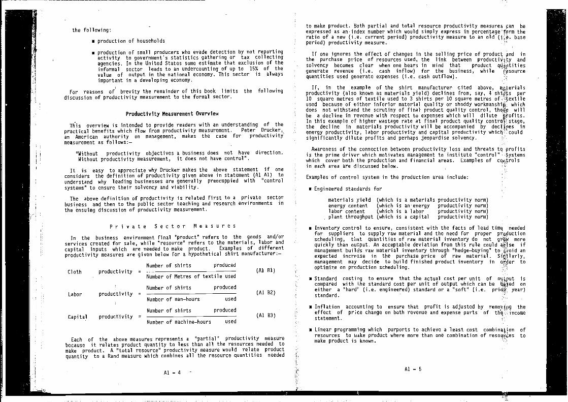
Chapter Al — THE PRODUCTIVITY CONCEPT
The purpose of this book is to bring to the attention of managers the notionof productivity and to expose them to a simplified form of a comprehensivemathematical structure (see Appendix B item A15 for the companionbook) which underpins proper productivity measurement. Simplyproductivity is the following quotient.
PRODUCT (i.e. OUTPUT) QUANTITYPRODUCTIVITY m (Al
RESOURCE (i.e. INPUT) QUANTITY
Whereas production refers to the conversion of resources comprising labor,material and capital (i.e. input) into goods and services of
a quotient which relates toa subset of resources used in the production process. Since usedin the production process extend beyond labor, the definition ofalso deals with resources other than labor. Yet labor plays a centrar rpl e,since capital and materials cannot produce anything unless labor theprocess. Although it is common to talk of productivity as output per oflabor input, it must be borne in mind that an increase in this canalso be driven by utilization of materials and capital
The author believes that managers should familiarise withproductivity and its proper measurement in view of the growing need fur thebenefits to be derived from productivity improvement. The relaflonshipbetween productivity measurement and productivity improvement is dftcussedin the ensuing chapter.
This chapter discusses the importance of promoting productivity growth,corrects common fallacies about the productivity concept, presents an q,jerviewof productivity measurement, identifies defects in conventionalmeasures and specifies characteristics for sound productivitywhich are satisfied by the approach defined in the companion techni4i bookcited above.
The Importance of Promoting Productivity Growth
Productivity is becoming a hot issue in the unpredictable,economic environment in which we live. It is increasingly recognized the
Al — 1
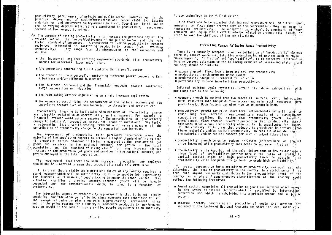
I11 productivity performance of private and public sector undertakings is theprincipal determinant of cost—effectiveness and hence viability. Leadingundertakings and government policy—makers in First, Second and Third Worldsare to varying degrees articulating a commitment to productivity improvementbecause of the rewards it brings.
C]\ The purpose of raising productivity is to increase the profitability of theJ private sector, the cost—effectiveness of thepublic sector and the realliving standard of consumers. A commitment to improve productivity createsaudiences interested in monitoring productivity trends (i.e. trackingproductivity). They range from the microcosm up to the macrocosm andinclude:
• the industrial engineer defining engineered standards (i.e productivitynorms) for labor and/or plant
• the accountant controlling a cost center within a profit center
i the product or group controller monitoring different profit centers withina business and/or different businesses
• the business economist and the financial/investment analyst monitoringlarge corporations or industries
• the rate—making officer adjudicating on a rate increase application
• the economist scrutinizing the performance of the national economy and itsunderlying sectors such as manufacturing, construction and services etc.
Productivity tracking is facilitated when measures of productivity changeare directly related to an operationally familiar measure, For example, afinancial officer would value a measure of the contribution of productivitychange to budgets for production, costs, net income or investment. Similarly,a rate—making (i.e., tariff—setting) tribunal would value a measure of the
• contribution of productivity change to the requested rate increase.
The improvement of productivity is of paramount importance where themajority of the population expects to achieve a higher standard of living thanit presently enjoys. Standard of living is measured as the consumption (ofgoods and services in the national economy) per person in the totalA\ population, and the standard of living cannot for long increase without
• increase in the production (of goods and services in the national economy) perperson employed in the total population.
The requirement that there should be increase in production per employeeshould not be construed to mean that productivity deals only with labor.
It is clear that a stable socio—political future of any country requires asound economy which will be sufficiently vigorous to provide job opportunityfor hundreds of thousands of people trying to enter the labor market. Thissituation signifies a growing economy. Economic growth will be largelydependent upon our competitiveness which, in turn, is a function ofproductivity.
The interesting aspect of productivity improvement is that it is not simplysomething for "the other party" to do, since everyone must contribute to it.The managerial cadre can play a key role in productivity improvement, sinceone of the prime reasons for a country's inadequate productivity performancemust be sought in the lack of highly skilled people together with an inability
Al — 2
to use technology to its fullest extent.
It is therefore to he expected that increasing pressure will be placed uponmanagers to focus their efforts more on the contributions they can make toincreasing productivity. The managerial cadre should be cognisant ofpressure and equip itself with knowledge related to productivity issues inorder to meet the challenge of the new situation.
Correcting Common Fallacies About Productivity
There is no commonly accepted intuitive definition of "productivity"there is, albeit imprecise, intuitive understanding of notions such as "bjm","unemployment", "inflation" and "profitability". It is thereforeto give cursory attention to the following examples of misleading rhetori&andhow they should be qualified:
• economic growth flows from a boom and not from productivity• productivity growth promotes unemployment• productivity change is irrelevant to inflation• profitability is niore important than productivity.
Informed opinion would typically correct the above ambiguities withpositions such as the following: -
• economic growth is derived from two potential sources, viz.,more resources into the production process and using such resources joreproductively. Both factors can give rise to an economic boom.
• productivity growth may cause short term retrenchments but will tocause long term increase in employment as a result of acompetitive position. The notion that productivity growth leads tounemployment flows from an incorrect perception that productivitydisplaces labor aione, specifically when capital is substituted forOn the contrary, it is clear that productivity growth can be derivedhigher materials and/or capital productivity. In this situation inthe materials and/or capital content per unit of output takes place.
• productivity growth tends to reduce inflation (defined here asprice increase) while productivity loss tends to increase inflation.
• productivity is the key, but not the sole, determinant of how sustainable agiven level of profitability (defined here as the ratio of tocapital assets) might be. High productivity tends to sustain sighprofitability while low productivity tends to erode high
To create perspective for a definition of productivity, one must ask whodetermines the level of productivity in the country. In a strict sense it istrue that anyone who works contributes to the productivity level thecountry as a whole. A comprehensive classification of the economy wguldreflect the following breakdown:
• formal sector, comprising all production of goods and services whichin the Sytem of National Accounts which is specified by internatiäpalconvention and which is subdivided into a private sector and asector.
• informal sector, comprising all production of goods and services notincluded in the System of National Accounts and which includes, inter alia,
Al — 3
the following:
• production of households
• production of small producers who evade detection by not reportingactivity to government's statistics gathering or tax collectingagencies. In the United States some estimate that exclusion of theinformal sector leads to an undercounting of up to 15% of thevalue of output in the national economy. This sector is alwaysimportant in a developing economy.
For reasons of' brevity the remainder of this book limits the followingdiscussion of productivity measurement to the formal sector.
Productivity Measurement Overview
This overview is intended to provide readers with an understanding of thepractical benefits which flow from productivity measurement. Peter Drucker,an American authority on management, makes the case for productivity'measurement as follows:—
"Without productivity objectives a business does not have direction.Without productivity measurement, it does not have control".
It is easy to appreciate why Drucker makes the above statement if one
considers the definition of productivity given above in statement (Al Al) tounderstand why leading businesses are generally preocuppied with "controlsystems" to ensure their solvency and viability.
The above definition of productivity is related first to a private sectorbusiness and then to the public sector teaching and research environments inthe ensuing discussion of productivity measurement.
Private Sector MeasuresIn the business environment final "product" refers to the goods and/or
services created for sale, while "resource" refers to the materials, labor andcapital inputs which are needed to make product. Examples of differentproductivity measures are given below for a hypothetical shirt manufacturer:—
Number of shirts producedCloth productivity = (Al Bl)
Labor productivity =
Capital productivity =
Number of shirts produced
Number of man—hours used
Number of shirts produced
Each of the above measures represents a "partial" productivity measurebecause it relates product quantity to less than all the resources needed tomake product. A "total resource" productivity measure would relate productquantity to a Rand measure which combines all the resource quantities needed
to make product. Both partial and total resource productivity measures beexpressed as an index number which would simply express in percetitage form theratio of a new (Le. current period) productivity measure to an old (j;e. baseperiod) productivity measure.
If one ignores the effect of changes in the selling price of product and inthe purchase price of resources used, the link between andsolvency becomes clear when one bears in mind that productgenerate revenue (i.e. cash inflow) for the business, whilequantities used generate expenses (i.e. cash outflow).
If, in the example of the shirt manufacturer cited above,productivity (also known as materials yield) declines from, say, 4 shk9s per10 square metres of textile used to 3 shirts per 10 square metres of7textileused because of either inferior material quality or shoddy workmanship whichdoes not withstand the scrutiny of final product quality control, willbe a decline in revenue with respect to expenses which will diluteIn this example of higher wastage rate at final product quality stage,the decline in materials productivity will be accompanied by inenergy productivity, labor productivity and capital productivitysignificantly dilute profits and perhaps jeopardise solvency.
Awareness of the connection between productivity loss and threats tq profitsis the prime driver which motivates management to institute "control"which cover both the production and financial areas. Examples of cqs',trolsin each area are discussed below.
materials yield (which is a materials productivity norm)energylaborplant
contentcontentthroughput
(which is anenergy(which is a labor(which is a capital
productivityproductivityproductivity
norm)norm)norm)
• Inventory control to ensure, consistent with the facts of lead time neededfor suppliers to supply raw material and the need for proper prcgJuctionscheduling, that quantities of raw material inventory do not morequickly than output. An acceptable deviation from this rule could ifmanagement builds raw material inventory through "hedge—buying" to floid anexpected increase in the purchase price of raw material. S4ilarly,management may decide to build finished product inventory in dSer tooptimize on production scheduling.
• Standard costing to ensure that the actual cost per unit of oqtput iscompared with he standard cost per unit of output which can be Uaed oneither a "hard' (i.e. engineered) standard or a "soft" (i.e. year)standard.
• Inflation accounting to ensure that profit is adjusted by theeffect of prce change on both revenue and expense parts of incomestatement.
• Linear programming which purports to achieve a least cost combinaL)on ofresources to product where more than one combination of tomake product is known.
Examples of control system in the production area include:
• Engineered star4ards for
(Al B2)
(Al B3)
Number of Metres of textile used
Al — 4Al — 5
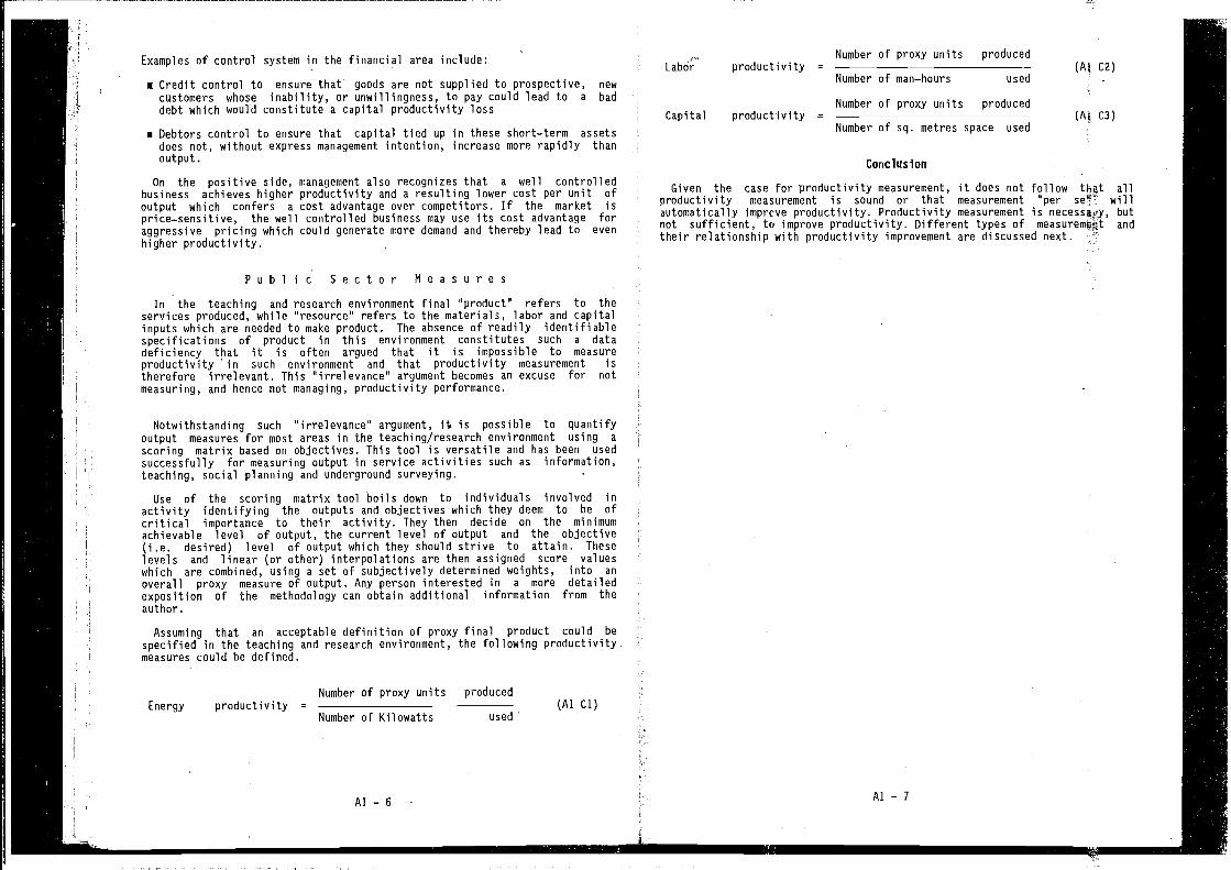
Examples of control system in the financial area include:
i Credit control to ensure that goods are not supplied to prospective, new
customers whose inability, or unwillingness, to pay could lead to a baddebt which would constitute a capital productivity loss
_________________________________
• Debtors control to ensure that capital tied up in these short—term assetsdoes not, without express management intention, increase more rapidly thanoutput. Conclusion
On the positive side, management also recognizes that a well controlledbusiness achieves higher productivity and a resulting lower cost per unit of Given the case for productivity measurement, it does not follow th4t alloutput which confers a cost advantage over competitors. If the market is productivity measurement is sound or that measurement 'per willprice—sensitive, the well controlled business may use its cost advantage for automatically imprcve productivity. Productivity measurement is necessagy, butaggressive pricing which could generate more demand and thereby lead to even not sufficient, to improve productivity. Different types of measuremeht and
higher productivity, their relationship with productivity improvement are discussed next. --
Public Sector MeasuresIn the teaching and research environment final "product" refers to the
services produced, while "resource" refers to the materials, labor and capitalinputs which are needed to make product. The absence of readily identifiablespecifications of product in this environment constitutes such a datadeficiency that it is often argued that it is impossible to measureproductivity in such environment and that productivity measurement istherefore irrelevant. This "irrelevance" argument becomes an excuse for notmeasuring, and hence not managing, productivity performance.
Notwithstanding such "irrelevance" argument, it is possible to quantifyoutput measures for most areas in the teaching/research environment using a
scoring matrix based on objectives. This tool is versatile and has been usedsuccessfully for measuring output in service activities such as information,teaching, social planning and underground surveying. -
Use of the scoring matrix tool boils down to individuals involved inactivity identifying the outputs and objectives which they deem to be ofcritical importance to their activity. They then decide on the minimumachievable level of output, the current level of output and the objective(i.e. desired) level of output which they should strive to attain. Theselevels and linear (or other) interpolations are then assigned score valueswhich are combined, using a set of subjectively determined weights, into an
overall proxy measure of output. Any person interested in a more detailedexposition of the methodology can obtain additional information from theauthor.
Assuming that an acceptable definition of proxy final product could be
specified in the teaching and research environment, the following productivity.measures could be defined.
Number of proxy units producedEnergy productivity = (Al Cl)
Number of Kilowatts used
Al—6 Al—7
-t
Number of proxy units producedLabor productivity = C2)
Number of man—hours used
Number of proxy units producedCapital productivity = (A! C3)
Number of sq. metres space used
Chapter A2 - PRODUCTIVITY IMPROVEMENT AND PRODUCTIVITY MEASUREMENT
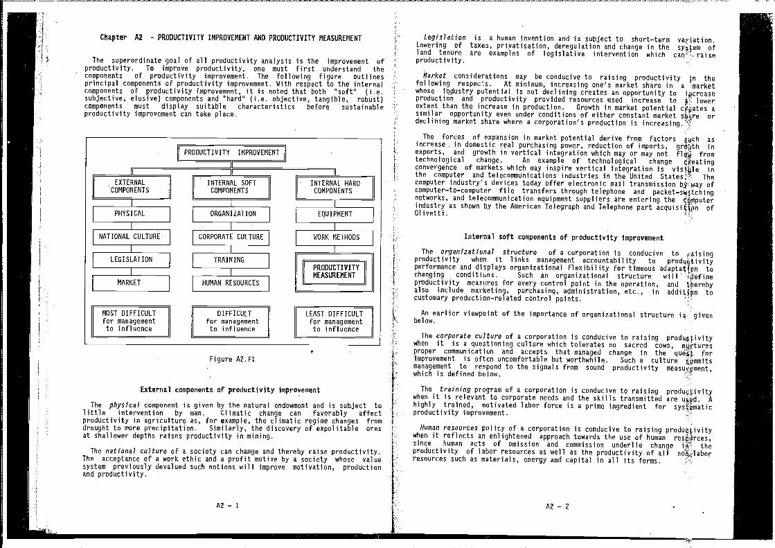
The superordinate goal of all productivity analysis is the improvement ofproductivity. To improve productivity, one must first understand thecomponents of productivity improvement. The following figure outlinesprincipal components of productivity improvement. With respect to the internalcomponents of productivity improvement, it is noted that both 'soft" (i.e.subjective, elusive) components and "hard" (i.e. objective, tangible, robust)components must display suitable characteristics before sustainableproductivity improvement can take place.
External components of productivity Improvement
The physical component is given by the natural endowment and is subject tolittle intervention by man. Climatic change can favorably affectproductivity in agriculture as, for example, the climatic regime changes fromdrought to more precipitation. Similarly, the discovery of expolitable oresat shallower depths raises productivity in mining.
The national culture of a society can change and thereby raise productivity.The acceptance of a work ethic and a profit motive by a society whose valuesystem previously devalued such notions will improve motivation, productionand productivity.
Legislation is a human invention and is subject to short—term variation.Lowering of taxes, privatisation, deregulation and change in the ofland tenure are examples of legislative intervention which raiseproductivity.
Market considerations may be conducive to raising productivity jn thefollowing respects. At minimum, increasing one's market share in a marketwhose industry potential is not declining creates an opportunity to Ipcreaseproduction and productivity provided resources used increase to lowerextent than the increase in production. Growth in market potential asimilar opportunity even under conditions of either constant market shire ordeclining market share where a corporation's production is increasing.
The forces of expansion in market potential derive from factors ;och asincrease in domestic real purchasing power, reduction of imports, inexports, and growth in vertical integration which may or may not fromtechnological change. An example of technological change
Fconvergence of markets which may inspire vertical integration is inthe computer and telecommunications industries in the United Thecomputer industry's devices today offer electronic mail transmission way ofcomputer—to—computer file transfers through telephone and packet—switching
• networks, and telecommunication equipment suppliers are entering the• industry as shown by the American Telegraph and Telephone part acquisitfon ofOlivetti.
Internal soft components of productivity Improvement
The organizational structure of a corporation is conducive to raisingproductivity when it links management accountability to prodqotivityperformance and displays organizational flexibility for timeous adaptat(pn tochanging conditions. Such an organizational structure will iiefineproductivity measures for every control point in the operation, andalso include marketing, purchasing, administration, etc., in additipn tocustomary production—related control points.
An earlier viewpoint of the importance of organizational structure is givenbelow.
The corporate culture of a corporation is conducive to raising productivitywhen it is a questioning culture which tolerates no sacred cows,proper communication and accepts that managed change in the quéi.j forimprovement is often uncomfortable but worthwhile. Such a culture {bmmitsmanagement to respond to the signals from sound productivitywhich is defined below.
The training program of a corporation is conducive to raisingwhen it is relevant to corporate needs and the skills transmitted are uud. Ahighly trained, motivated labor force is a prime ingredient forproductivity improvement.
Human resources policy of a corporation is conducive to raisingwhen it reflects an enlightened approach towards the use of humansince human acts of omission and commission underlie change i11 theproductivity of labor resources as well as the productivity of allresources such as materials, energy and capital in all its forms.
k
Figure A2.F1
A2—1 A2—2
Internal hard components of productivity improvement
The equipment (and supporting technology) used by a corporation are
conducive to raising productivity when they are the best available which can
be economically justified.
The work methods used by a corporation are conducive to raising productivitywhen they are the best available which can be economically justified. Work
methods include the following engineering ("hard system") approaches towards
improving operations: Value engineering, just—in—time, group technology, total
quality control, multiple resource planning, computer aided design, computer
aided manufacture, and so forth.
The productivity measurement system used by a corporation is conducive to
raising productivity when it is the best available which can be economically
justified. Deterministic and stochastic approaches to productivity
measurement are defined below as a prelude to a discussion of the strengths
and weaknesses of different types of productivity measurement.
Deterministic and stochastic approaches to measurement
Deterministic approaches to measurement start by defining certain equations
as axioms or identities (i.e. relationships which are always valid) and then
proceed to derive other relationships from transformations of the initialaxioms. A deterministic model permits total accuracy provided initial axioms
can be specified and the model can be populated with credible data.
Stochastic approaches to measurement start with the assumption that axioms
are not known to define the relationship in question. Stochastic approaches
therefore resort to probablistic equations which employ regressions (i.e.statistical inferences) to estimate a relationship which is not known with
certainty. A stochastic methodology is justified and plays an indispensable
role only when a deterministic one cannot be identified.
The approach presented in this volume is deterministic. The preference of
the engineering and accounting communities for rigor, precision and freedom
from ambiguity indicated at an early stage a need to develop, as far as
possible, a deterministic methodology in lieu of a stochastic one. Business
economists, industrial engineers and accountants have long used deterministic
models to appraise the performance of the individual producer establishment.
Yet the reader with econometrics training may be surprised to encounter in
this book some novel deterministic specifications in areas where stochasticspecifications are customarily found in econometric literature.
The author offers no apology for this fact, and points out that the adoption
of a stochastic methodology implies that a deterministic one cannot be
identified. On the contrary, the practitioners of stochastic methodology, for
those types of analysis for which a deterministic methodology has now been
identified, will be obliged to justify their stochastic practice.
General weakness and strength of all productivity measurement
A general weakness of all productivity measurement arises from the fact thatthe productivity quotient has no necessary causal significance. Changes in
productivity express effect and not cause. Causal insight can only be provided
by those familiar with a given operation. Ongoing productivity measurement,
known as productivity tracking, therefore poses rather than answers questions.
A2 — 3
A general strength of all productivity measurement with toproductivity improvement. efforts arises from its overall monitor as
attempts are made to change soft and hard components cited above. Ato improve productivity creates a need for productivity measurement.
productivity measurement there would be no score—card to ascertainsystematic efforts to raise productivity are bearing any fruit.
Productivity measurement is a hard component of productivity irlipregement
which can quantify the effect of productivity change on financialThe soft components must be activated to enable management to proceedeffect and thereby uncover cause so that remedial action to improvecan be formulated and implemented.
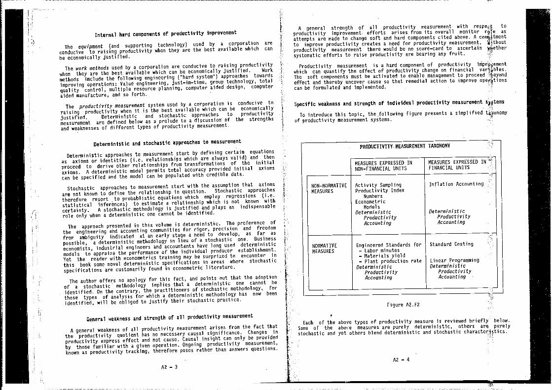
Specific weakness and strength of individual productivity measurement
To introduce this topic, the following figure presents a simplified tgAonomyof productivity measurement systems.
I
PRODUCTIVITY. MEASUREMENT TAXONOMY
MEASURES EXPRESSED INNON—FINANCIAL UNITS
•1
- MEASURES EXPRESSED INFINANCIAL UNITS
NON—NORMATIVE
MEASURES
Activity SamplingProductivity Index
NumbersEconometPi c
ModelsDeterministic
ProductivityAccounting
Inflation Accounting
DeterministicProductivityAccounting
NORMATIVEMEASURES
Engineered Standards for— Labor minutes— Materials yield— Plant production rate
DeterministicProductivityAccounting
Standard Costing
Linear ProgrammingDeterministic
ProductivityAccounting
Each of theSome of thestochastic and
Figure A2.F2
above types of productivity measure is reviewed briefly below.above measures are purely deterministic, others are purelyyet others blend deterministic and stochastic characterbtics.
AZ — 4
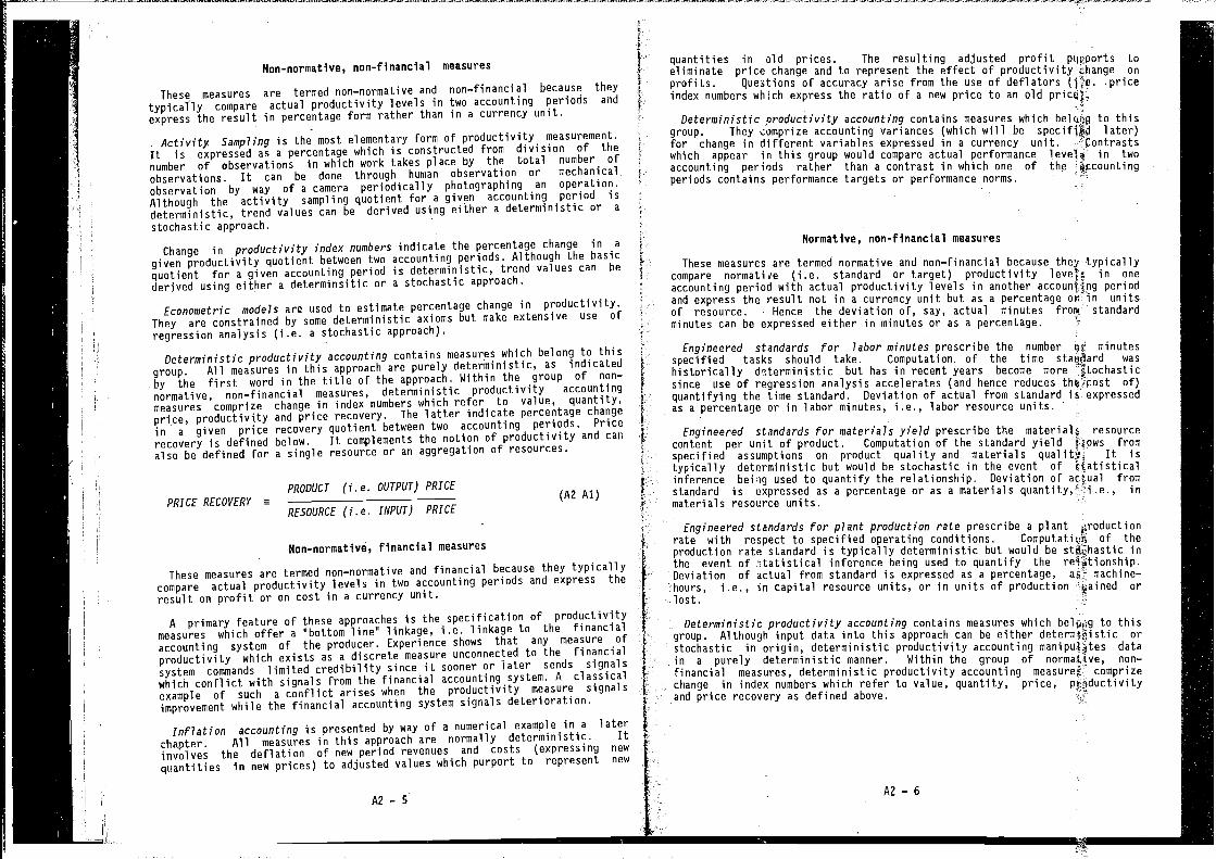
Non-norñiatiVe, non-financial measures
These measures are termed non—normative and non—financial because they
typically compare actual productivity levels in two accounting periods and
express the result in percentage form rather than in a currency unit.
Activity Sampling is the most elementary form of productivity measurement.
It is expressed as a percentage which is constructed from division of the
number of observations in which work takes place by the total number of
observations. It can be done through human observation or mechanical
observation by way of a camera periodically photographing an operation.
Although the activity sampling quotient for a given accounting period isdeterministic, trend values can be derived using either a deterministic or a
stochastic approach.
Change in productivity index numbers indicate the percentage change in a
given productivity quotient between two accounting periods. Although the basic
quotient for a given accounting period is deterministic, trend values can be
derived using either a determinsitic or a stochastic approach.
Econometric models are used to estimate percentage change in productivity.
They are constrained by some deterministic axioms but make extensive use of
regression analysis (i.e. a stochastic approach).
Deterministic productivity accounting contains measures which belong to this
group. All measures in this approach are purely deterministic, as indicated
by the first word in the title of the approach. Within the group of non—
normative, non—financial measures, deterministic productivity accounting
measures comprise change in index numbers which refer to value, quantity,price, productivity and price recovery. The latter indicate percentage change
in a given price recovery quotient between two accounting periods. Price
recovery is defined below. It complements the notion of productivity and canalso be defined for a single resource or an aggregation of resources.
PRDDUCT (i.e. DUTPUT) PRICEPRICE RECDVERY a
(A2 Al)RESDURCE (i.e. INPUT) PRICE
Non-normative, financial measures
These measures are termed non—normative and financial because they typicallycompare actual productivity levels in two accounting periods and express the
result on profit or on cost in a currency unit.
A primary feature of these approaches is the specification of productivitymeasures which offer a "bottom line" linkage, i.e. linkage to the financial
accounting system of the producer. Experience shows that any measure of
productivity which exists as a discrete measure unconnected to the financial
system commands limited credibility since it sooner or later sends signals
which conflict with signals from the financial accounting system. A classical
example of sqch a conflict arises when the productivity measure signalsimprovement while the financial accounting system signals deterioration.
Inflation accounting is presented by way of a numerical example in a laterchapter. All measures in this approach are normally deterministic. Itinvolves the deflation of new period revenues and costs (expressing new
quantities in new prices) to adjusted values which purport to represent new
quantities in old prices. The resulting adjusted profit pqrports toeliminate price change and to represent the effect of productivity ihange on
profits. Questions of accuracy arise from the use of deflators (Uè. .priceindex numbers which express the ratio of a new price to an old pricej.
Deterministic productivity accounting contains measures which to thisgroup. They comprise accounting variances (which will be specifj4d later)for change in different variables expressed in a currency unit.which appear in this group would compare actual performance leveh in twoaccounting periods rather than a contrast in which one of the accountingperiods contains performance targets or performance norms.
Normative, non-financial measures
These measures are termed normative and non—financial because they typicallycompare normative (i.e. standard or target) productivity in oneaccounting period with actual productivity levels in another accoun%(ng periodand express the result not in a currency unit but as a percentage oWin unitsof resource. Hence the deviation of, say, actual minutes frop4 standardminutes can be expressed either in minutes or as a percentage.
Engineered standards for 7abor minutes prescribe the number minutesspecified tasks should take. Computation. of the time sta&ard was
historically drterministic but has in recent years become more
since use of regression analysis accelerates (and hence reduces of)quantifying the time standard. Deviation of actual from standard is expressedas a percentage or in labor minutes, i.e., labor resource units. I
Engineered standards for materials yield prescribe the resourcecontent per unit of product. Computation of the standard yield fiows fromspecified assumptions on product quality and materials It istypically deterministic but would be stochastic in the event of hiatisticalinference being used to quantify the relationship. Deviation of acçual fromstandard is uxpressed as a percentage or as a materials quantityj:i.e., inmaterials resource units.
Engineered standards for plant production rate prescribe a plant productionrate with respect to specified operating conditions. of theproduction rate standard is typically deterministic but would be inthe event of 5tatistical inference being used to quantify the re44ionship.Deviation of actual from standard is expressed as a percentage, machine—
hours, i.e., in capital resource units, or in units of production orlost.
Deterministic productivity accounting contains measures which to thisgroup. Although input data into this approach can be either determjoistic orstochastic in origin, deterministic productivity accounting datain a purely deterministic manner. Within the group of normative, non-financial measures, deterministic productivity accounting measuret comprisechange in index numbers which refer to value, quantity, price,and price recovery as defined above.
A2—6A2-5
I
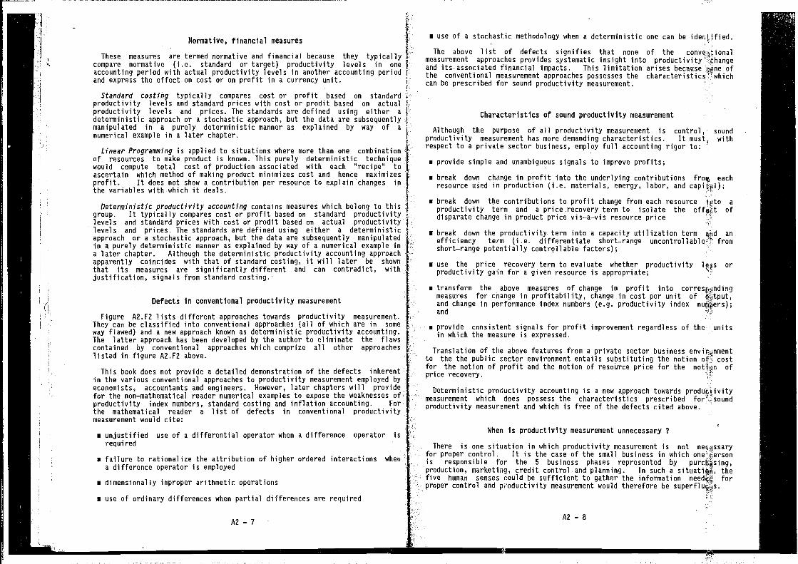
Normative, financial measures
These measures are termed normative and financial because they typicallycompare normative (i.e. standard or target) productivity levels in oneaccounting period with actual productivity levels in another accounting periodand express the effect on cost or on profit in a currency unit.
Standard costing typically compares cost or profit based on standardproductivity levels and standard prices with cost or prodit based on actualproductivity levels and prices. The standards are defined using either a
deterministic approach or a stochastic approach, but the data are subsequentlymanipulated in a purely deterministic manner as explained by way of a
numerical example in a later chapter. -
Linear Programming is applied to situations where more than one combinationof resources to make product is known. This purely deterministic techniquewould compute total cost of production associated with each "recipe" toascertain which method of making product minimizes cost and hence maximizesprofit. It does not show a contribution per resource to explain changes inthe variables with which it deals.
Deterministic productivity accounting contains measures which belong to thisgroup. It typically compares cost or profit based on standard productivitylevels and standard prices with cost or prodit based on actual productivitylevels and prices. The standards are defined using either a deterministicapproach or a stochastic approach, but the data are subsequently manipulatedin a purely deterministic manner as explained by way of a numerical example ina later chapter. Although the deterministic productivity accounting approachapparently coincides with that of standard costing, it will later be shownthat its measures are significantly different and can contradict, withjustification, signals from standard costing.
Defects in conventional productivity measurement
Figure A2,F2 lists different approaches towards productivity measurement.They can be classified into conventional approaches (all of which are in someway flawed) and a new approach known as deterministic productivity accounting.The latter approach has been developed by the author to eliminate the flawscontained by conventional approaches which comprize all other approacheslisted in figure A2.F2 above.
This book does not provide a detailed demonstration of the defects inherentin the various conventional approaches to productivity measurement employed byeconomists, accountants and engineers. However, later chapters will providefor the non—mathematical reader numerical examples to expose the weaknesses ofproductivity index numbers, standard costing and inflation accounting. Forthe mathematical reader a list of defects in conventional productivitymeasurement would cite:
• unjustified use of a differential operator when a difference operator isrequi red
• failure to rationalize the attribution of higher ordered interactions whena difference operator is employed
• dimensionally improper arithmetic operations
• use of ordinary differences when partial differences are required
• use of a stochastic methodology when a deterministic one can be
The above list of defects signifies that none of themeasurement approaches provides systematic insight into productivityand itsassociated financial impacts. This limitation arises because ofthe conventional measurement approaches possesses thecan be prescribed for sound productivity measurement.
Characteristics of sound productivity measurement
Although the purpose of all productivity measurement is control, soundproductivity measurement has more demanding characteristics. It withrespect to a private sector business, employ full accounting rigor to:
• provide simple and unambiguous signals to improve profits;
• break down change in profit into the underlying contributions froip eachresource in production (i.e. materials, energy, labor, and
i break down the contributions to profit change from each resource iHto a
productivity term and a price recovery term to isolate the ofdisparate change in product price vis—a—vis resource price
• break down the productivity- term into a capacity utilization term qud anefficiency term (i.e. differentiate short—range fromshort—range potentially controll able factors);
• use the price recovery term to evaluate whether productivity lqs orproductivity gain for a given resource is appropriate;
• transform the above measures of change in profit intomeasures for cnange in profitability, change in cost per unit ofand change in performance index numbers (e.g. productivity indexand
• provide consistent signals for profit improvement regardless of the- unitsin which the measure is expressed.
Translation of the above features from a private sector businessto the the public sector environment entails substituting the notion costfor the notion of profit and the notion of resource price for the notldn ofprice recovery. -
Deterministic productivity accounting is a new approach towards productivitymeasurement which does possess the characteristics prescribed soundproductivity measurement and which is free of the defects cited above.
When is productivity measurement unnecessary ?
There is one situation in which productivity measurement is notfor proper control. It is the case of the small business in whichis responsible for the 5 business phases represented by
• production, marketing, credit control and planning. In such a situatthji, thefive human senses could be sufficient to gather the information forproper control and productivity measurement would therefore be
A2 — 8A2 — 7
•
•1.
Productivity measurement is merely a component of the productivityimprovement process which is holistic by nature. If isolated from other softcomponents discussed above, productivity measurement will fail to thrive and
in consequence not contribute to productivity improvement. The processwhereby managers could strive to pilot the migration of an organisation fromproductivity measurement to productivity improvement is described by theproductivity management journey in the next chapter.
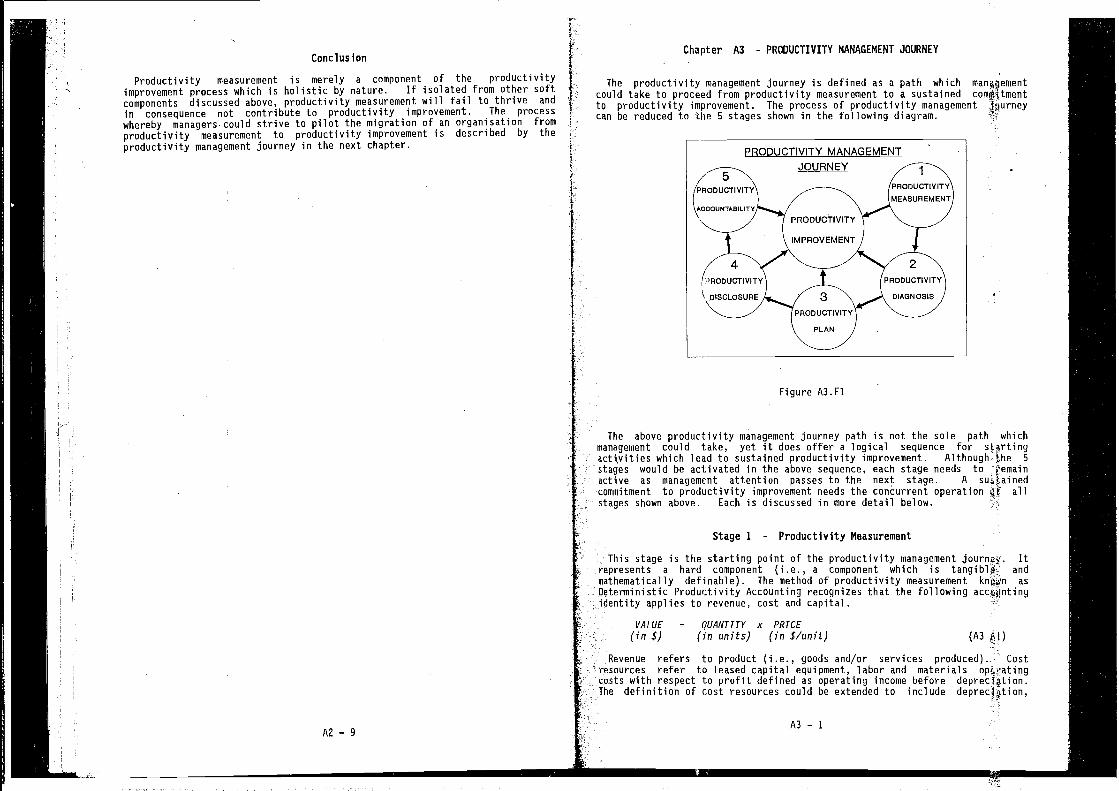
The productivity management journey is defined as a path whichcould take to proceed from productivity measurement to a sustainedto productivity improvement. The process of productivity managementcan be reduced to the 5 stages shown in the following diagram.
The above productivity management journey path is not the sole path whichmanagement could take, yet it does offer a logical sequence for startingactivities which lead to sustained productivity improvement. Although 5
stages would be activated in the above sequence, each stage needs toactive as management attention passes to the next stage. A
commitment to productivity improvement needs the concurrent operation allstages shown above. Each is discussed in more detail below.
Stage 1 - Productivity Measurement
This stage is the starting point of the productivity management journey. Itrepresents a hard component (i.e., a component which is andmathematically definable). The method of productivity measurement asDeterministic Productivity Accounting recognizes that the followingidentity applies to revenue, cost and capital.
VALUE = QUANTITY x PRICE(in 5) (in units) (in s/unit) (A3 fl)
Revenue refers to product (i.e., goods and/or services produced). Costresources refer to leased capital equipment, labor and materialscosts with respect to profit defined as operating income beforeThe definition of cost resources could be extended to include deprec4flion,
Chapter A3 - PRODUCTIVITY MANAGEMENT JOURNEYConclusion
PRODUCTIVITY MANAGEMENT
Figure A3.F1
A2—9A3—l
interest paid and other finance—related charges with respect to profit defined
as taxable income. Capital resources refer to fixed capital assets and to
working capital assets.
Deterministic Productivity Accounting employs the above value axiom to
derive various other axioms which include the following:
PRODUCT QUANTITY
PRODUCTIVITY a(A3 Bi)
RESOURCE QUANTITY
PRODUCT PRICE
PRICE RECOVERY a(A3 Cl)
RESOURCE PRICE
The above measures are then applied to uncover the financial effect of,
inter alia, productivity change and price recovery change of each cost
resource and capital resource used in a given operation.
The limitation of all productivity measurement is that it focusses on effect
rather than cause and is therefore a mechanism for posing rather than
answering questions. The strength of Deterministic Productivity Accounting is
that it provides an overall financial monitor of all systematic effort to
raise productivity.
Stage 2 - Productivity Diagnosis
This stage represents a soft component (i.e., a component which is
intangible and cannot be mathematically defined). It strives to proceed
beyond effect to uncover cause and hence to explain the reasons for
productivity change. Its strength is that it attempts to answer questions
posed by measurement, Yet it will fail whenever the corporate cultureresists ascertainment of cause.
Success in the productivity diagnosis stage depends upon management's
ability to create and nurture an open, questioning culture in which there are
no sacred cows to which the cause of productivity improvement can be held
hostage. Quality circles which are effective can be an example of such
desirable attributes in the corporate culture of an organization.
Stage 3 - Productivity Plan
This stage represents hard and soft components. Using the insights gained
by productivity diagnosis, this stage strives to formulate a productivity plan
which identifies what changes are needed to move the organization from itscurrent productivity levels to target productivity levels which are specified
in this stage and which are included in budgets.
A productivity plan typically contains hard components which includes
equipment, measures such as key performance ratios, productivity and price
recovery targets, as well as other engineering—based hard systems such as
value engineering, multiple resource planning and just—in—time control
systems. A productivity plan also contains soft components (i.e., changes in
organization, training and culture). This stage requires a clear specificationof objectives, strategy and tactics needed in the soft components to ensure
that the hard components of the plan will be achieved. It would also
A3 - 2
introduce productivity measurement as an overall financial monitor of effortto raise productivity.
Stage 4 Productivity Disclosure
This stage represents a hard component. It involves disclosing tg internaland external audiences the family of grids defined byProductivity Accounting as the profit grid, productivity grid, grid,price grid and cost grid. The grids preserve confidentiality of nuSric dataand simply show position with respect to defined segments in jach grid.Disclosure of the grids could start with internal audiences and ththteafter beextended to include external audiences.
Disclosure to internal audiences within the organization creates •awarenessof the productivity concept, assists its assimilation within the corporateculture and prepares the organization for the major step ofdisclosure to external audiences. External audiences are intended functionas a proxy for competition in markets where there are few In thecase of a private sector undertaking the external audience investorsand consumers, whereas in the case of a public sector a
central or local government body, the external audience comprizes :taxpayersand consumers.
Productivity disclosure to external audiences represents the acid test ofmanagement commitment to the notion of productivity Onceinitiated, this stage cannot easily be revoked and will inevitably to thefollowing stage.
Stage 5 - Productivity Accountability
This stage represents a soft component. It involvesaccountability for productivity performance disclosed by the grids specifiedabove.
Specifically, it relates to actual productivity performance well as
planned productivity performance. Actual productivity wouldrelate! actual productivity in a given accounting period to that indicated by
either a prior actual accounting period or a budget for theperiod. Planned productivity performance would relate planned ina given budget to that indicated by either a prior actual
a prior accounting period.
Irrespective of the signal from the grids at the time of initial disclosureto an external audience, management stands to gain credit from the action ofexternal disclosure. If the initial grids signal inproductivity, management is praised for candor in disclosing dfleriorationand, by inference, for committing itself to reverse the direction f$om one ofdeterioration to one of improvement in productivity. On the hand, ifthe initial gvids signal improvement in productivity, management :4p praisedfor good performance and, by inference, for committing itself sustainimprovement in productivity.
Management accountability for disclosed productivity willmotivate management to respond to signals from ongoing fl4ductivitymeasurement, productivity diagnosis and productivity planning. - In otherwords, productivity accountability will induce management to walkdown the path of productivity improvement. -
A3 — 3
C
The Outcome - Productivity Improvement
This stage represents hard and soft components. It will not be possible toattain and maintain productivity improvement unless hard and soft componentscited above are continually melded together. Productivity improvement wouldbe detected through productivity measurement and communicated to stakeholdersthrough productivity disclosure. Stakeholders are defined as suppliers,producers and consumers. Suppliers include the suppliers of labor, materialsand capital resources. In the case of the private sector investors supplyinvestment capital and are included in the definition of suppliers. In thecase of the public sector taxpayers supply investment capital and are includedin the definition of suppliers.
A disclosed, healthy productivity and price recovery track record would tendto reduce uninformed consumer resistance to increase in product price from a
private business, increase in utility rate from a rate—regulated utility orincrease in tax rate from central or local government. Instead it offersobjective facts which indicate the extent to which the producer achievesproductivity growth to finance the absorption of resource price increase whichhe does not recover from consumers by way of an increase in the product price,utility rate or tax rate. Hence the difference between the resource priceincrease and that which is recovered from the consumer would constitute priceunder—recovery and the transfer of a subsidy from the producer to theconsumer.
Conclusion
The productivity management journey contains hard and soft components. Itcan determine the extent of sustainable productivity improvement and hencecompetitive strength, the safety of the investment and the extent to which theproducer can afford to subsidise the consumer.
The productivity management journey can be usefully compared with themanagement of the flight path of an aircraft in the following manner. The
flight of an aircraft is managed by the pilot who is dependent upon bothdirect sensing devices, which provide data on fuel supply, speed etc., andremote sensing devices such as a radar altimeter which provides data on heightabove the earth, Throughout the flight altimetry provides ongoinginformation on the changing topographical features of the earth surface belowthe aircraft. The pilot can elect to disregard remotely sensed altimetricdata and thereby imperil the aircraft.
p
Similarly, the role of productivity measurement is to provide remote sensingof the financial consequences of the changing productivity terrain whicharises from movement of the organization through time and space. The managercan elect to disregard remotely sensed productivity data and thereby imperilthe organization.
Both altimetry and productivity measurement represent hard components withsoft objectives. They seek, respectively, to influence the decision behaviourpattern of the pilot managing the flight path of the aircraft and the managercharged with managing the productivity journey of the organization.
Success in the soft and hard components described in chapter A2 will impactupon productivity and hence financial performance as monitored bydeterministic productivity accounting. In the productivity management journeyproductivity measurement should therefore be seen as a background activity todetect productivity change and calibrate efforts to improve productivity.
A3—4
Chapter A4 - HOW MEASUREMENT ASSISTS PRODUCTIVITY MANAGEMENT
The purpose of this chapter is to define in practise how measurementprovides information to enable management to make better decisions,operations and progress along the productivity management journey.
Productivity Diagnosis for Management
The total resource productivity measurement approach described in this bookmeasures the profit contribution of each resource in terms of capacityutilization, efficiency, and price recovery. Using this information candiagnose which resources contribute significantly to higher profit potágtialwhich can be attained by better allocation of resources. k-
The price recovery term for each resource is used to determineproductivity gain or loss is appropriate for that resource. Subject t( anyappropriate constraints, resources making the less favorable toprice recovery should be targeted for productivity growth (i.e., reduced usageper unit of output) which must more than offset any trade—off productIvityloss (i.e., increased usage per unit of output) from resources making tha'morefavorable contributions to price recovery.
It is appropriate to contrast short term price recovery with efficiency (forshort—term control cycles). It is also appropriate to contrast long, termprice recovery with productivity (for long—term control cycles) since ip thelong term, all resources are variable and, hence, controllable. - Thiscomparison permits the systematic substitution of cheap resources forexpensive resources to optimize profit consistent with the length of thecontrol cycle. Since this approach provides bottom—line measures of chanfl incapacity utilization, efficiency, and price recovery for eachmanagement can pinpoint where productivity improvement efforts will thegreatest beneficial impact on the business.
Some corporations have attempted to analyze their productivity usingconventional approaches such as partial production measures, totalproductivity index numbers, inflation accounting, and/or standard Tcostaccounting. None of these conventional measurement approaches, howk.ver,provides systematic insight into productivity change and itsfinancial impacts. This limitation arises because none of the conventionalmeasurement approaches possesses the characteristics that can befor sound productivity measurement as specified in chapter A2 thediscussion of Characteristics of sound productvity measurement.
Management Control
The approach presented in this book shows that it is possible to thebottom—line impact of change in productivity and change in price recovery foreach resource used in the operation of a business. This fact hassignificance because it permits management to gauge the bottom—line dellareffect of change in the allocation of individual resources withincontrol points. This argument is explained below with respect to bgth alow level control print and a higher level control point.
Even if it is unable to influence price recovery because of itsto control product and resource prices, management at a low level cöwtrolpoint such as a production control point has some prospect of
A4 — 1
the efficiency term in the productivity change. Management at a low levelcontrol point which offers no control of price recovery can still use the
price recovery measure to validate its targets for productivity change.
Sound productivity targeting requires a net positive tradeoff from
changes in resource allocation which give rise to productivity gain
on resources which are used less intensively and to productivity loss on
resources which are used more intensively as a result of planned
substitutions. Business profit improves when relatively cheaper resources
are substituted for relatively dearer resources.
The price recovery variance per resource enables management to determine
whether resources making the least favorable contribution to price recoveryare targeted for productivity growth.- Productivity growth is achieved by
tolerating less than offsetting productivity loss in resources making a more
favorable contribution to price recovery. In this manner the price recovery
variance is used to validatE the direction of productivity change for each
resource.
The sign and magnitude of the bottom—line impact of the price recovery
variance for each resource can send different types of signals to various
levels of control points in a business. For example, negative pricerecovery for a given resource signifies that product price increase does notrecover the extent of price increase for that resource. From this signaldifferent control points may draw the following types of inference.
• A production control point may infer that it should strive throughresource reallocation to target that resource for productivitygrowth (i.e., reduced usage per unit of production).
• A purchasing control point may infer that it should strive, ifpossible, to lower the specification for that resource to achieve a
favorable purchasing variance.
• A production planning control point may infer that it should explore
a make—versus—buy option for that resource, and this analysis may
identify technological gaps that the research and development functioncould explore.
Existing control systems explore the above questions by way of discreteinitiatives which drive specific studies of these questions. The
proposed control system would expliciXly integrate the price recovery
signal, with its decomposition by resource, into the basic profit variance
analysis which is seen by management. This would help management focus
on what questions it should be asking on the setting of productivitytargets for selected individual resources or sets of resources.
At a higher level control point which makes decisions on both production
and product pricing, management may trade price recovery variance offagainst productivity variance in the following manner. If a product
experiences a price elasticity of demand greater than positive unity,management may decide to reduce product price (and hence opt for less
A4 — 2
favorable price recovery variance) to generate more—than—offsettjpg profitfrom production volume (and hence opt for more favorableproductivity variance which flows principally from improvqG capacityutilization).
This possibility of measuring for each resource the ofproductivity change and price recovery change to change in profit, suggeststhat their agjregation permits explaining the origin of in theincome statement as portrayed in the 9—box diagram on the cover book,
Summary
Profitability can be described as the result of the contribution of pricerecovery and productivity. Although management cannot always pricerecovery, it can always influence productivity. The first step influenceproductivity contributions of all resources used is to adopt a soun4 method bywhich they can be measured.
Sound productivity measurement possesses characteristics (a,j specifiedearlier) which should underpin all systematic efforts to raiseregardless of whether those efforts originate from high—level contSl pointssuch as the management committee or low—level control points such as costcenter expense budgets in a plant.
The model discussed above and the PM software implementation of the model
used in this book provide an analytical tool that can be used validateother studies focusing on improving productivity through such as
vertical integration, investment, technological change,incentive schemes, and training.
• A financialintegrationunattractiveprofitabilityquestion.
planningshould be
on costin the
control point may inferinvestigated if the make
grounds and there existsbusiness sector supplying the
that reverseoption is
acceptableresource in
L
A4 — 3
PART B — INPUT FUNCTIONS
part of the book presents the following chapter.
Chapter 81 DATA REQUIREMENTS AND DEFAULT VALUES
Chapter Bi DATA REQUIREMENTS AND DEFAULT VALUES
The 10 input functions (i.e. user specified functions) required by the modelare defined in this chapter. If the user fails to provide informationby the model, use is made of either default values (which are definedchapter) or proxy values (which are defined in Part G of the book).
The distinction between default values and proxy values is soajçwhatarbitrary, but is nonetheless clearly defined. With the exception of thefunction TARGET RETURN ON IN VESTMENT, whose default value is set at oldintrinsic return on investment, all default values of input functions setat 0 or at 1. In contrast, proxy values assume a wider range ofvalues as shown in Part 0.
The 10 input functions required from the user are specified in stateRents(81 Al) through (81 32).
Q (QUANTITY FUNCTION) is a user specified functibn.(81 Al)
dimension is typically given in physical units.(81
The above suite of statements refers to the level of a function. It dbtinesthe Quantity function which is specifed by the user on the basic partitthr ofaccounting data. This function is dimensioned and is typically expressed insome physical unit such as tons, work—hours etc. It is defined forand resource.
There is no default value for the quantity function, and its proxy valutc isdefined in Part.G of the book. 2
P (PRICE FUNCTION) is a user specified function.(81 hI)
P dimension is given in currency unit / physical units.(81
The above suite of statements refers to the level of a function. It detjnesthe Price function which is specifed by the user on the basic partitin ofaccounting data. This function is dimensioned and is typically insome currency unit divided by physical units. It is defined for product andresource.
There is no default value for the price function, and its proxy isdefined in Part 0 of the book.
81—1
W (INTERVAL WIDTH FUNCTION) is a user specified function.
W dimension is given in days or other unit of time.
(81 Cl)
(81 C2)
The above suite of statements refers to the level of a function. It definesthe user specified interval Width. This function is dimensioned and istypically expressed in some unit of time such as hours, shifts or days of a
given intensity. This feature of the model would, for example, allow a chainstore user to weight, say, a Saturday with a greater intensity than a Monday.This function is defined for product and resource.
Function W is important in the following two cases:
— high frequency control cycles (i.e., a month and shorter periods), sinceit is misleading to compare, say, an 18 workday month such as Februarywith a 22 workday month such as March.
— a change in th.e closing month for an accounting year could give rise todiffering numbers of months per year when the last of the old years andthe first of the new years are compared.
The following entity rule of function W is implemented in the axioms and isspecified below:
Function W is applied to function Q(U), i.e., product Quantity
Function W is applied to function Q(N), i.e., cost resource Quantity
Function W is applied to function T(K,), i.e., target rate of returnin turn applied toP(K) representingresource asset Price.
The value functions for revenue (i.e., product value), operating expense(i.e., cost resource value) and target profit (i.e., cost of capital) allcontain a time component in contrast with the value function for capitalassets (i.e., capital asset value) which is time free. In other wordsreve4lile, cost and target profit values are time bound since they refer to a
flow concept with respect to a time interval such as a month, quarter or yearwhereas asset value is time free since it refers to a point concept such as
the value at close of business on the last business day within such timeinterval
Given the axiom Value = Quantity * Price, a value function which has a timecomponent in the left hand expression creates a need to distribute the timecomponent to either the quantity function or the price function in the righthand expression. The above entity rule of function W signifies that the timecomponent in the value function is distributed to the quantity function forproduct and cost resources, and to the price function for capital resourcesvia function T (for Target return on investment) in a manner which is shown inthe following figure.
In the following figure, RAW DATA refers to the form of data at source,while DATA ENTRY refers to how data must be transformed before entry todistribute the time component from the value function to the quantity functionor the price function according to the entity rule of W specified above.
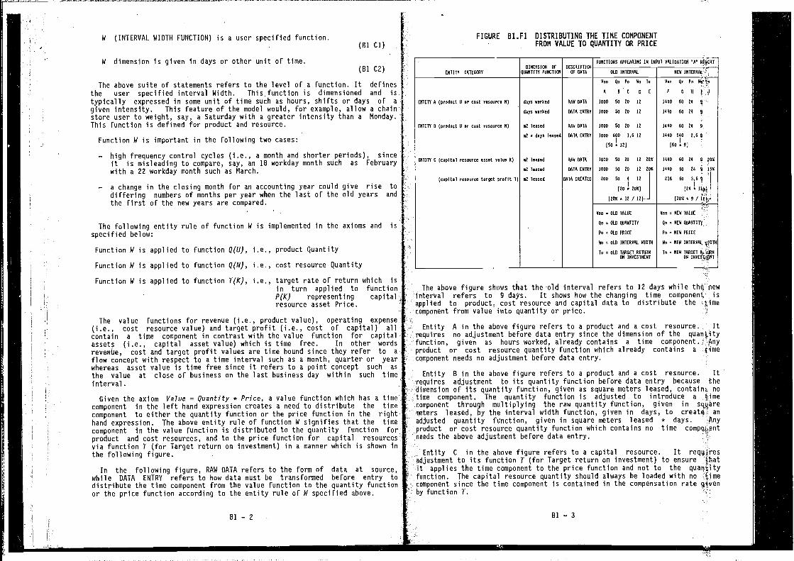
FIGURE B1.F1 DISTRIBUTING THE TIME COMPONENTFROM VALUE TO QUANTITY OR PRICE
ENTITY CAIEIONYDINENSION OF
QUANTITY FUNCTIONDESCRIPTIV4
OF DATA
FUNCTIONS APPEARING IN INPUT
OLD INTERAAL
VALIDATION NtAC41T
NEN
ENTITY 0 (product U or cost roosore, N) deys worked VAN DATA
Roe Qo Ps No To
A DC DC1000 DO 1D ID
Von Re Po
F OR1440 60 DO
days worked DOTA ENTVV DODD 10 DD ID 1440 NO D4
ENTDTT D (product U or coot rooource N) ml leased RAN DATA 1000 00 20 Il 1440 60 24 5
ml o doyo Teased DATA ENTRY 1000 ADO 16 Il[10 a Il]
1440 040 0,0
[60 0 4]
ENTITY C (capital reooorce wooeD 'jaDe, K)
(capital reoeerce taroet profit T)
ml leased
ml leased
ml loosed
RAN DATA
DATA ENTRY
DATA CREATED
1000 50 DO ID 20%
1000 10 20 Il 200
200 50 4 Il[20 o 00%)
[lOO0ll/lD)_J
1440 60 04 !INRO 00 24 ISO
216 00 3,0
[00 a
)lOTeD/l&I.
Poe = OLD VALUE One NEA VALUE
Re = OLD QUANTITY Qe = NEW QUANTITY
Po OLD PRICE Pn = NCA P01CC
Ne = OLD INTERVAL 01010
To = OLD TVROET VETOONON INVESTMENT
An NEW INTERVAL
Tn NEW TAOOET RAVURNON
The above figure shows that the old interval refers to 12 days while thg pewinterval refers to g days. It shows how the changing time component isapplied to productn cost resource and capital data to distribute the ttimecomponent from value into quantity or price.
Entity A in the above figure refers to a product and a cost resource. Itrequires no adjustment before data entry since the dimension of the quantityfunction, given as hours worked, already contains a time component.product or cost resource quantity function which already contains a fleeComponent needs no adjustment before data entry.
Entity B in the above figure refers to a product and a cost resource. Itrequires adjustment to its quantity function before data entry because thedimension of its quantity function, given as square meters leased, containt notime component. The quantity function is adjusted to introduce a timecomponent through multiplying the raw quantity function, given in sqparemeters leased, by the interval width function, given in days, to create. anadjusted quantity function, given in square meters leased * days. fryproduct or cost resource quantity function which contains no time compqt5entneeds the above adjustment before data entry.
Entity C in the above figure refers to a capital resource. It requiresadjustment to its function T (for Target return on investment) to ensure thatit applies the time component to the price function and not to thefunction. The capital resource quantity should always be loaded with no timecomponent since the time component is contained in the compensation rate givenby function T.
81—2 81—3
which iSfunctioncapital
The default value for the width function W is I unit of time. The modeluses the quotient of new interval width and old interval width and therebycreates a quotient of dimensionless unity when I unit of time is entered for,say, each of two years containing 365 days. A default value would bewhen the user specifies a quantity function but omits to specify a widthfunction. Proxy values for the width function arise when a proxy product or a
proxy cost resource is required, as specified in Part G of the book.
T is a dimensionless function.
(Cl DI)
(Cl D2)
The above suite of statements refers to the level of a function. It definesthe user specified Target return on investment which is used to define thetarget profit level by individual element of capital investment. It is definedonly for capital resources.
The default value for both old target return on investment and new targetreturn on investment is the function for old intrinsic return on investmentwith respect to a specified contrast. It is used when the user specifiescapital asset value but omits to specify a target return on investment. A
proxy value for target return on investment arises when proxy capital isrequired, as specified in Part G of the book.
S (RISK WEIGHT FOR INVESTMENT) is a user specified function.
S is a dimensionless function.
(Cl El)
(Cl E2)
The above suite of statements refers to the level of a function. It definesthe user specified risk weight on investment which is one of the functionsused to distribute the intrinsic profit level to the individual elements ofcapital investment.
The default value for risk weight for investment is dimensionless unity. Itis used when the user specifies capital quantity and price but omits tospecify a risk weight for investment. A proxy value for the risk weight forinvestment arises when proxy capital is required, as specified in Part G ofthe book.
REM (RESOURCE VARIABILITY RATIO) is a user specified function.
REV/i is a dimensionless function.(Cl F2)
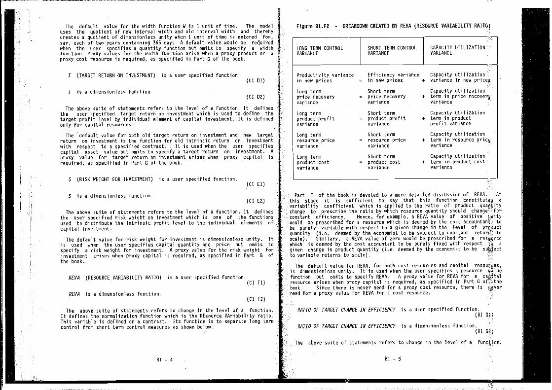
The above suite of statements refers to change in the level of a function.It defines thenormalization function which is the REsource VAriability ratio.This variable is defined on a contrast. Its function is to separate long termcontrol from short term control measures as shown
Part F of the book is devoted to a more detailed discussion of REVA. Atthis stage it is sufficient to say that this function constitutes a
variability coefficient which is applied to the ratio of product quafltitychange to prescribe the ratio by which resource quantity should change forconstant efficiency. Hence, for example, a REVA value of positive unitywould be prescribed for a resource which is deemed by the cost tobe purely variable with respect to a given change in the level ofquantity (i.e. deemed by the economist to be subject to constant returii toscale). Similary, a REVA value of zero would be prescribed for a resiurcewhich is deemed by the cost accountant to be purely fixed with respect a
given change in product quantity (i.e. deemed by the economist to be subjectto variable returns to scale).
The default value for REVA, for both cost resources and capitalis dimensionless unity. It is used when the user specifies a resourcefunction but omits to specify REVA. A proxy value for REVA for a caAitalresource arises when proxy capital is required, as specified in Part Gbook. Since there is never need for a proxy cost resource, there isheed for a proxy value for REVA for a cost resource.
B1—4 Bl—5
U
T (TARGET RETURN ON INVESTMENT) is a user specified function.
Figure B1.F2 -. BREAKDOWN CREATED BY REVA (RESOURCE VARIABILITY RATIQI
LONG TERM CONTROL SHORT TERM CONTROL CAPACITY UTILIZATIONVARIANCE VARIANCE VARIANCE
Efficiency variance Capacity utilization= in new prices + variance in new
Productivity variancein new prices
Long termprice recoveryvan ance
Long termproduct profitvan ance
Long termresource pricevariance
Long termproduct costvariance
Short term= price recovery
variance
Short term= product profit
variance
Short term= resource price
variance
Short term= product cost
variance
Capacity utilization+ term in price recovery
variance -
Capacity utilization+ term in product
profit variance
Capacity utilization+ term in resource
variance
Capacity utilization+ term in product cost
variance
(Cl Fl)
RATIO OF TARGET ClAP/GE IN EFFICIENCY is a user specified function.(BI Gi)
RATIO OF TARGET C/lANGE IN EFFICIENCY is a dimensionless function.(Bl Ga)
The above suite of statements refers to change in the level of a function.
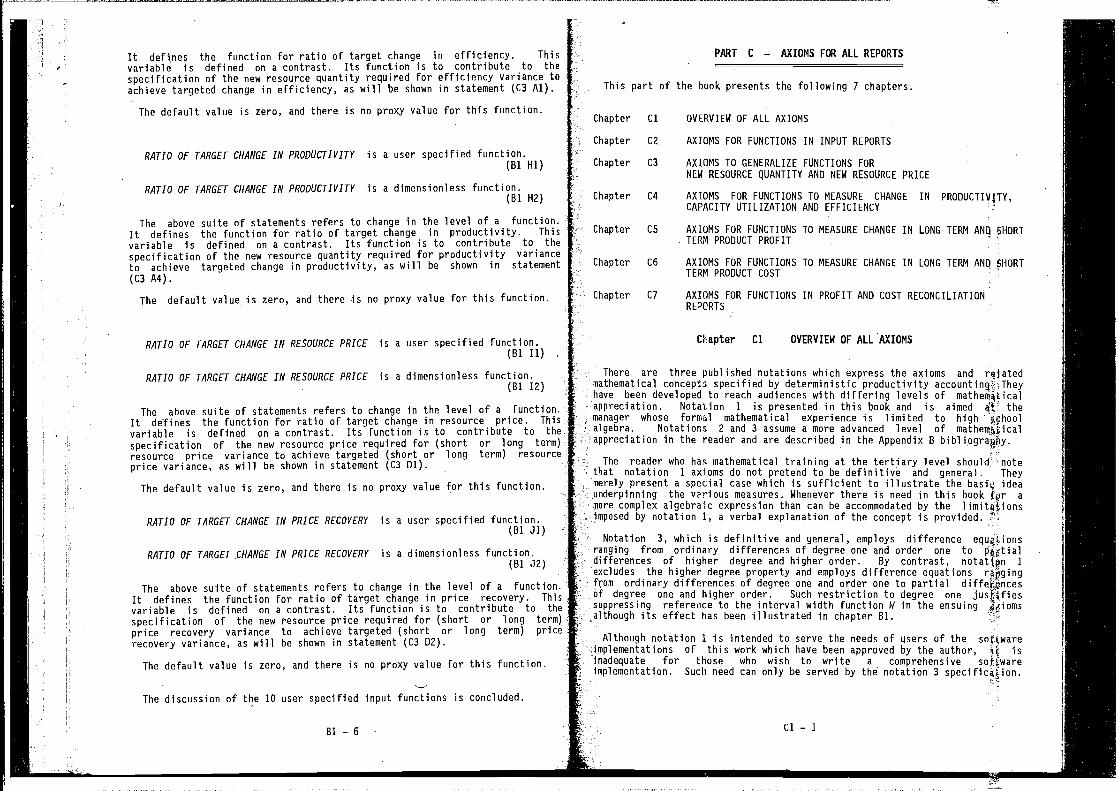
It defines the function for ratio of target change in efficiency. Thisvariable is defined on a contrast. Its function is to contribute to thespecification of the new resource quantity required for efficiency variance toachieve targeted change in efficiency, as will be shown in statement (C3 Al).
The default value is zero, and there is no proxy value for this function.
RATIO OF TARGET CHANGE IN PRODUCTIVITY is a user specified function.(Bl Hl)
RATIO OF TARGET CHANGE IN PROOUCTIVITY is a dimensionless function.(Bl H2)
The above suite of statements refers to change in the level of a function.It defines the function for ratio of target change in productivity. Thisvariable is defined on a contrast. Its function is to contribute to thespecification of the new resource quantity required for productivity varianceto achieve targeted change in productivity, as will be shown in statement(C3 A4).
The default value is zero, and there is no proxy value for this function.
RATIO OF TARGET CHANGE IN RESOURCE PRICE is a user specified function.(Bl Ii)
RATIO OF TARGET CHANGE IN RESOURCE PRICE is a dimensionless function.(Bl 12)
The above suite of statements refers to change in the level of a function.It defines the function for ratio of target change in resource price. Thisvariable is defined on a contrast. Its function is to contribute to thespecification of the new resource price required for (short or long term)resource price variance to achieve targeted (short or long term) resourceprice variance, as will be shown in statement (C3 Dl).
The default value is zero, and there is no proxy value for this function.
RATIO OF TARGET CHANGE IN PRICE RECOVERY is a user specified function.(B1 J1)
RATIO OF TARGET CHANGE IN PRICE RECOVERY is a dimensionless function.(BI J2)
The above suite of statements refers to change in the level of a function.It defines the function for ratio of target change in price recovery. Thisvariable is defined on a contrast. Its function is to contribute to thespecification of the new resource price required for (short or long term)price recovery variance to achieve targeted (short or long term) pricerecovery variance, as will be shown in statement (C3 02).
The default value is zero, and there is no proxy value for this function.
The discussion of the 10 user specified input functions is concluded.
Bl—6
PART C — AXIOMS FOR ALL REPORTS
This part of the book presents the following 7 chapters.
Chapter Cl OVERVIEW OF ALL AXIOMS
Chapter C2 AXIOMS FOR FUNCTIONS IN INPUT REPORTS
Chapter C3 AXIOMS TO GENERALIZE FUNCTIONS FORNEW RESOURCE QUANTITY AND NEW RESOURCE PRICE
Chapter C4 AXTONS FOR FUNCTIONS TO MEASURE CHANGE IN PRODUCTIVITY,CAPACITY UTILIZATION AND EFFICIENCY
Chapter C5 AXIOMS FOR FUNCTIONS TO MEASURE CHANGE IN LONG TERM ANQ SHORTTERM PRODUCT PROFIT
Chapter C6 AXIOMS FOR FUNCTIONS TO MEASURE CHANGE IN LONG TERM ANQ SHORTTERM PRODUCT COST
Chapter C7 AXIOMS FOR FUNCTIONS IN PROFIT AND COST RECONCILIATIONREPORTS
Chapter Cl OVERVIEW OF ALL AXIOMS
There are three published notations which express the axioms and rglatedmathematical concepts specified by deterministic productivity Theyhave been developed to reach audiences with differing levels ofappreciation. Notation I is presented in this book and is aimed themanager whose formal mathematical experience is limited to highalgebra. Notations 2 and 3 assume a more advanced level of matheniflicalappreciation in the reader and are described in the Appendix B bibliography.
The reader who has mathematical training at the tertiary level should notethat notation I axioms do not pretend to be definitive and general. Theymerely present a special case which is sufficient to illustrate the basiv ideaunderpinning the v?rious measures. Whenever there is need in this book fur a
more complex algebraic expression than can be accommodated by the limitAtionsimposed by notation 1, a verbal explanation of the concept is provided.
Notation 3, which is definitive and general, employs differenceranging from ordinary differences of degree one and order one to pfltialdifferences of higher degree and higher order. By contrast, Iexcludes the higher degree property and employs difference equationsfrom ordinary differences of degree one and order one to partialof degree one and higher order. Such restriction to degree onesuppressing reference to the interval width function W in the ensuingalthough its effect has been illustrated in chapter BI.
Although notation I is intended to serve the needs of users of the softwareimplementations of this work which have been approved by the author, isinadequate for those who wish to write a comprehensiveimplementation. Such need can only be served by the notation 3
k
Cl — 1

Cell
(5) , (6)
Report
Input Validation "A" Report
Input Compact Report
C2—2
I Chapter C2 AXIOMS FOR FUNCTIONS IN INPUT REPORTS
This chapter presents axioms for the 6 Input Reports implemented in the 1988software release of determinstic productivity accounting. Examples of theaxioms and their reports appear in chapters [1 through E6.
INTRINSIC PROFIT
This measure refers to the level of a function, and its dimensionalcoefficient is a currency unit. Numerical examples for old and new intervalsappear in the following references.
Chapter Cell Report
El (1) , (2) Input Validation "A" Report
E5 Input Compact Report
The following two axioms are self—explanatory. The second expressions ineach axiom provide the mneumonic for the functions which appear in the firstexpression.
OLD INTRINSIC PROFIT a OLD TOTAL REVENUE - OLD TOTAL COST RESOURCES
PRDFITo7d a REVENUEoId — COSTo7o'(C2 El (1))
NEW INTRINSIC PROFIT a NEW TOTAL REVENUE — NEW TOTAL COST RESOURCES
PRDFITneW a REVENUEnew — CDSTnew(C2 El (2))
The words OLD and NEW refer to different accounting periods employed for a
contrast. They could be two historical periods, two forecast (i.e., budget)periods, any permutation of historical and forecast data for a givenoperation, or two different operations making similar product with respect toany permutation of historical and forecast data.
The following axioms define the average intrinsic return on investment fortotal capital resources valued at asset valuation as distinct from targetprofit valuation.
INTRINSIC RETURN ON INVESTMENT
This measure refers to the level of a function, and its dimensionalcoefficient is dimensionless. Numerical examples for old and new intervalsappear in the following references which explain the significance of the timecomponent introduced by the intrinsic profit dividend (i.e., numerator).
Chapter Cell Report
El (3) , (4) Input Validation "A" Report
ES Input Compact Report
OLD INTRINSIC PROFITCo a
OLD TOTAL ASSET VALUE OF CAPITAL RESOURCES (K ROWS)
(C2 ci (3))WHERE Co = OLD INTRINSIC (ACTUAL) RETURN ON INVESTNENT
NEW INTRINSIC PROFITCn a
NEW TOTAL ASSET VALUE OF CAPITAL RESOURCES (K ROWS)
(C2 Rj (4))WHERE Co = NEW INTRINSIC (ACTUAL) RETURN ON INVESTMENT
TARGET PROFIT VALUE
This measure refers to the level of a function, and itscoefficient is a currency unit. Numerical examples for old and new irflervalsappear in the following references.
Chapter
El
ES
The following axioms define the target profit for each capital asset. Thismeasure defines a dollar cost value of capital assets per unit of time whichplaces capital and cost resources on to the same footing. Henceforth it willbe possible to treat capital and cost resources in exactly the same forpurposes of productivity measurement and analysis.
OLD TARGET PROFIT VALUE (Ti)
a OLD CAPITAL ASSET VALUE (Xi) * OLD TARGET RETURN ON CAPITAL
= Vo(Ki) *To(C2 El (5))
NEW TARGET PROFIT VALUE (Ti)
a NEW CAPITAL ASSET VALUE (Ki) * OLD RETURN ON CAPITAL
= Via (Xi) *. To
(C2 (6))
TARGET PROFIT PRICE
This measure refers to the level of a function, and itscoefficient is a currency unit divided by the dimension to which thequantity refers. Numerical examples for old and new intervals thefollowing references.
Chapter Cell Report
El (7) , (8) Input Validation "A" Report
ES Input Compact Report
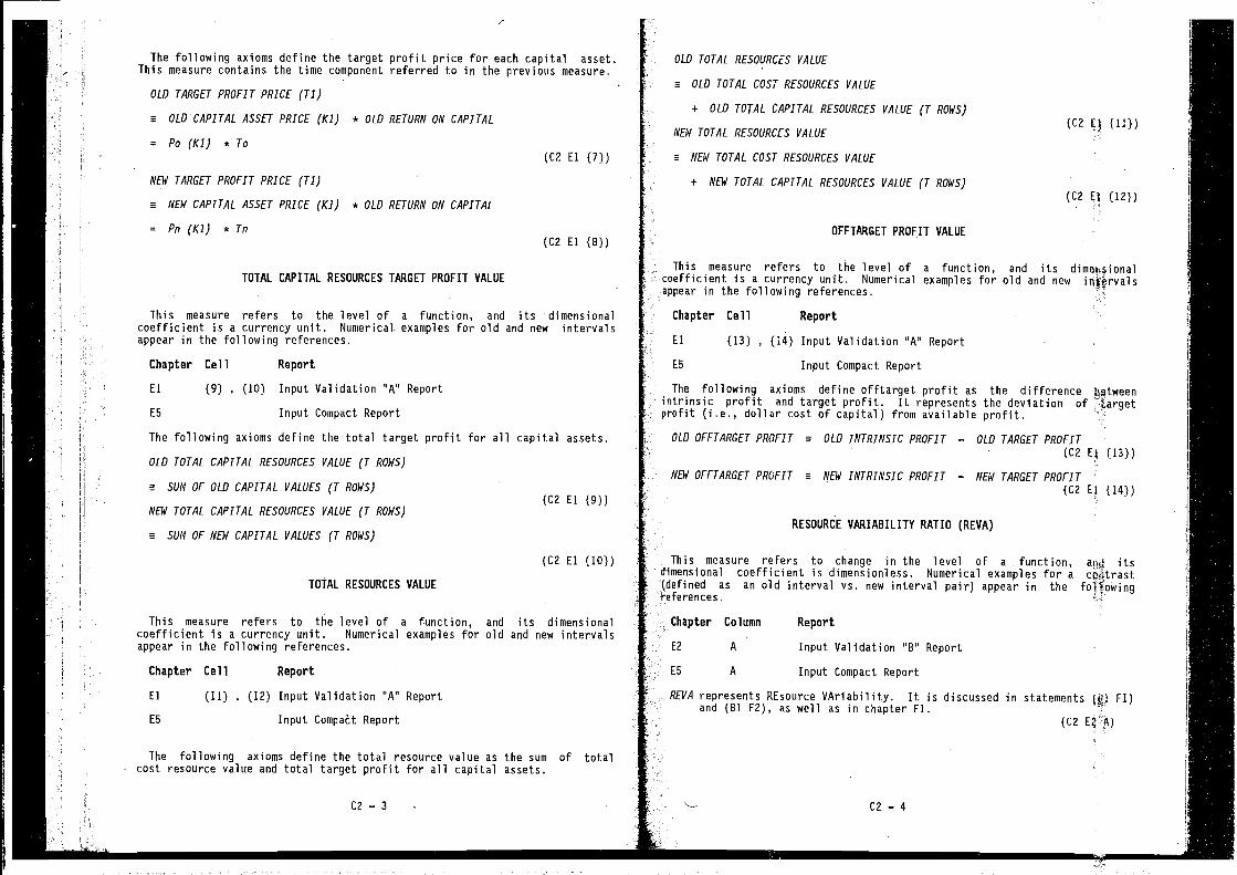
This measure refers to the level of a function, and its dimensionalcoefficient is a currency unit. Numerical, examples for old and new intervalsappear in the following references.
Chapter Cell Report
El (9) , (10) Input Validation 'A' Report
E5 Input Compact Report
The following axioms define the total target profit for all capital assets.
OLD TOTAL CAPITAL RESOURCES VALUE (T ROWS)
a SUM OF OLD CAPITAL VALUES (T ROWS)(C2 El (9))
MEW TOTAL CAPITAL RESOURCES VALUE (T ROWS)
a SUM OF NEW CAPITAL VALUES (T ROWS)
TOTAL RESOURCES VALUE
This measure refers to the level of a function, and its dimensionalcoefficient is a currency unit. Numerical examples for old and new intervalsappear in the following references.
Chapter Cell Report
El (11) , (12) Input Validation 'A' Report
E5 Input Report
The following axioms define the total resource value as the sum of totalcost resource value and total target profit for all capital assets.
This measure refers to the level of a function,coefficient is a currency unit. Numerical examples forappear in the following references.
Chapter Cell Report
El (13) , (14) Input Validation 'A' Report
E5 Input Compact Report
The following axioms define offtarget profit as the difference betweenintrinsic profit and target profit. It represents the deviation of 'targetprofit (i.e., dollar cost of capital) from available profit.
OLD OFFTARGET PROFIT m OLD INTRINSIC PROFIT — OLD TARGET PROFIT(C2 Ei (13))
C2—3 C2—4
The following axioms define the target profit price for each capital asset.This measure contains the time component referred to in the previous measure.
OLD TARGET PROFIT PRICE (Ti)
m OLDCAPITAL ASSET PRICE (Ki) * OLD RETURN ON CAPITAL
= Po (Ki) * To(C2 El (7))
NEW TARGET PROFIT PRICE (Ti)
m NEW CAPITAL ASSET PRICE (Ki) * OLD RETURN ON CAPITAL
= Pn(Ki) *Tn(C2 El (8))
TOTAL CAPITAL RESOURCES TARGET PROFIT VALUE
OLD TOTAL RESOURCES VALUE
m OLD TOTAL COST RESOURCES VALUE
+ OLD TOTAL CAPITAL RESOURCES VALUE (T ROWS)
NEW TOTAL RESOURCES VALUE
m NEW TOTAL COST RESOURCES VALUE
+ NEW TOTAL CAPITAL RESOURCES VALUE (T ROWS)
OFFTARGET PROFIT VALUE
(C2 EJ (11))
(C2 (12))
and itsold and new
(C2 El (10))
NEW OFFTARGET PROFIT a NEW INTRINSIC PROFIT — NEW TARGET PROFIT(C2 (14))
RESOURCE VARIABILITY RATIO (REVA)
This measure refers to change in the level of a function, aod itsdimensional coefficient is dimensionless. Numerical examples for a(defined as an old interval vs. new interval pair) appear in the foTTowingreferences.
Chapter Column Report
E2 A Input Validation "B' Report
E5 A Input Compact Report
REVA represents REsource VAriability. It is discussed in statements Fl)and (Bl F2), as well as in chapter Fl.
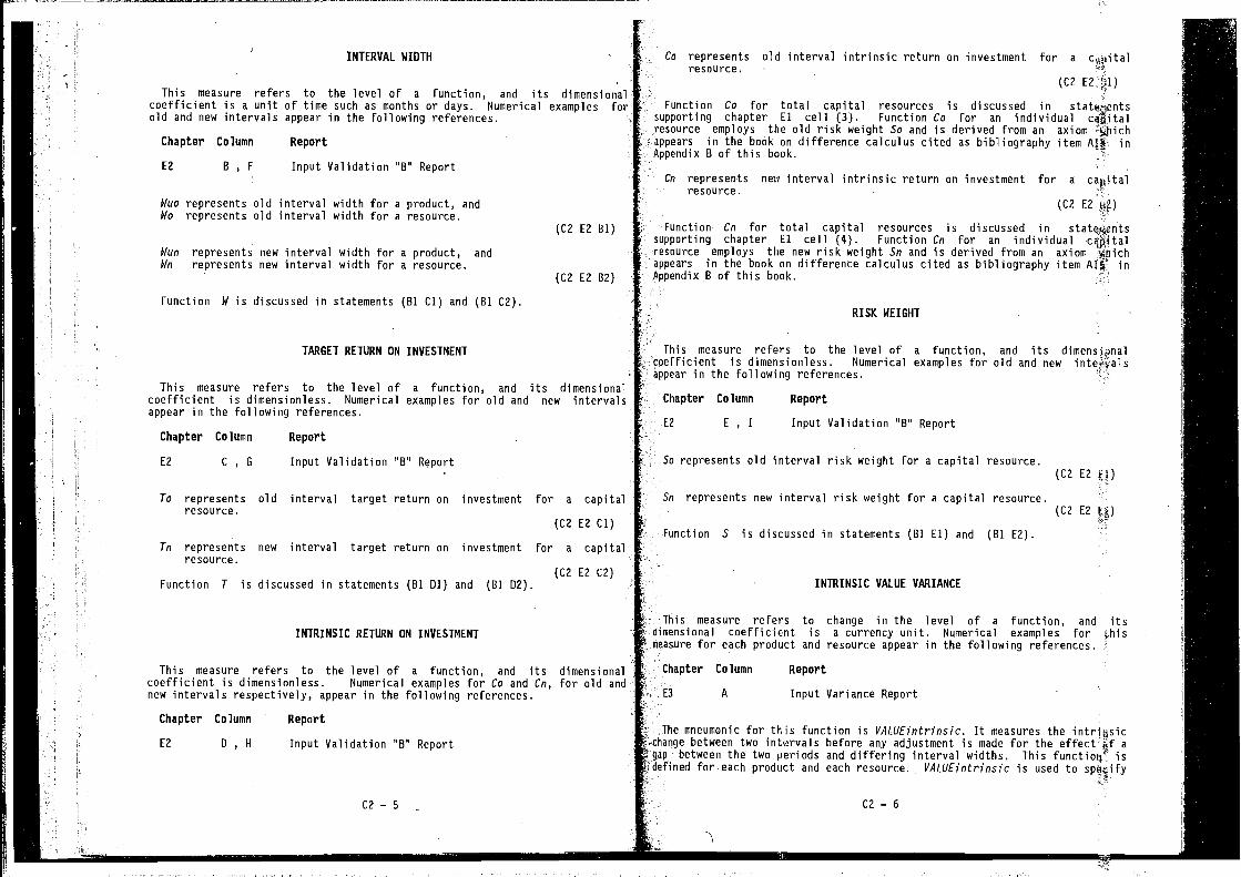
INTRINSIC RETURN ON INVESTMENT
This measure refers to the level of a function, and its dimensionalcoefficient is dimensionless. Numerical examples for Co and Cn, for old andnew intervals respectively, appear in the following references.
Chapter Column Report
E2 D , H Input Validation "B" Report
RISK WEIGHT
This measure refers to the level of a function, and itscoefficient is dimensionless. Numerical examples for old and new
in the following references.
Chapter Column Report
E2 E , I Input Validation "B" Report
So represents old interval risk weight for a capital resource.
Sn represents new interval risk weight for a capital resource.
Function S is discussed in statements (Bi El) and (Bi E2).
INTRINSIC VALUE VARIANCE
This measure refers to change in the level of a function, and itsdimensional coefficient is a currency unit. Numerical examples formeasure for each product and resource appear in the following references.
Chapter Column Report
E3 A Input Variance Report
The mneumonic for this function is VALUEintrinsic. It measures the intribsic• change between two intervals before any adjustment is made for the effectjf a
- gap between the two periods and differing interval widths. This functiow isdefined for.each product and each resource. V/lLUEintrinsfc is used to specify
C2—5 C2—6
Co represents old interval intrinsic return on investment for aresource.
• (C2
Function Co for total capital resources is discussed insupporting chapter El cell (3). Function Co for an individual cqitalresource employs the old risk weight So and is derived from an axiomappears in the book on difference calculus cited as bibliography item inAppendix B of this book.
Co represents new interval intrinsic return on investment for a ca&talresource.
(C2 E2 LiE)
Function Cn for total capital resources is discussed in statqthentssupporting chapter El cell (4). Function Cn for an individualresource employs the new risk weight Sn and is derived from an axiom jjhichappears in the book on difference calculus cited as bibliography item inAppendix B of this book,
INTERVAL WIOTH
This measure refers to the level of a function, and its dimensionalcoefficient is a unit of time such as months or days. Numerical examples forold and new intervals appear in the following references.
Chapter Column Report
E2 B , F Input Validation "B" Report
Wuo represents old interval width for a product, andWo represents old interval width for a resource.
(C2 E2 Bl)
Wun represents new interval width for a product, andWn represents new interval width for a resource.
(C2 E2 B2)
Function W is discussed in statements (Bl Cl) and (Bl C2).
TARGET RETURN ON INVESTMENT
This measure refers to the level of a function, and its dimensionalcoefficient is dimensionless. Numerical examples for old and new intervalsappear in the following references.
Chapter Column Report
E2 C , C Input Validation "B" Report
To represents old interval target return on investment for a capitalresource.
(C2 E2 Cl)
Tn represents new interval target return on investment for a capitalresource.
(C? E2 C2)Function T is discussed in statements (Bl Dl) and (Bl D2).
(C2 E2
(C2 E2
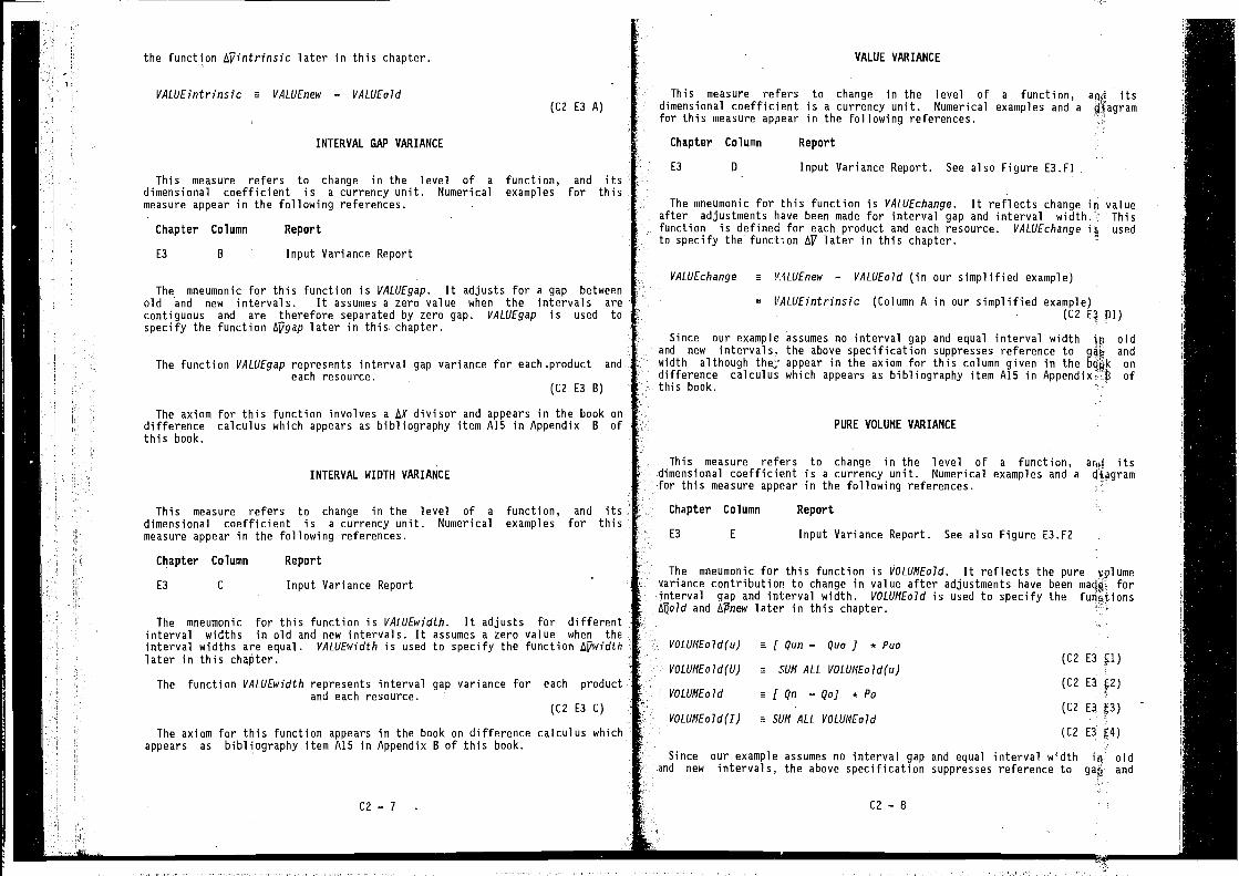
the function I$7intrinsic later in this chapter. VALUE VARIANCE
VALUEintrinsic a VALUErieW — VALUEo1d(C2 E3 A)
INTERVAL GAP VARIANCE
This measure refers to change in the level of a function, and itsdimensional coefficient is a currency unit. Numerical examples for thismeasure appear in the following references.
Chapter Column Report
E3 B Input Variance Report
The mneumonic for this function is VALUEgap. It adjusts for a gap betweenold and new intervals. It assumes a zero value when the intervals arecontiguous and are therefore separated by zero gap. VALUEgap is used tospecify the function Ajigap later in this chapter.
The function VALUEgap represents interval gap variance for each.product andeach resource.
(C2 E3 B)
The axiom for this function involves a AX divisor and appears in the book ondifference calculus which appears as bibliography item A15 in Appendix B ofthis book.
INTERVAL WIDTH VARIANCE
This measure refers to change in the level of a function, and itsdimensional coefficient is a currency unit. Numerical examples for thismeasure appear in the following references.
Chapter Column Report
E3 C Input Variance Report
The mneumonic for this function is VALUEwIdth. It adjusts for differentinterval widths in old and new intervals. It assumes a zero value when theinterval widths are equal. VALUEwidth is used to specify the function lit/widthlater in this chapter.
The function VALUEwidth represents interval gap variance for each productand each resource.
(C2 E3 C)
The axiom for this function appears in the book on difference calculus whichappears as bibliography item A15 in Appendix B of this book.
C2—7
This measure refers to change in the level of a function, aQj itsdimensional coefficient is a currency unit. Numerical examples and a çjlagramfor this measure appear in the following references.
Chapter Column Report
E3 D Input Variance Report. See also Figure E3.F1
The mneumonic for this function is VALUEchange. It reflects change in valueafter adjustments have been made for interval gap and interval width. Thisfunction is defined for each product and each resource. VALUEchaoge usedto specify the function AV later in this chapter.
VALUEchange a VALUEnew — VALUEo1d (in our simplified example)
= VALUEintrinsic (Column A in our simplified example)(C2 P1)
Since our example assumes no interval gap and equal interval width jn oldand new intervals, the above specification suppresses reference to andwidth although the; appear in the axiom for this column given in the bcjblc ondifference calculus which appears as bibliography item A15 in Appendix/B ofthis book.
PURE VDLUNE VARIANCE
This measure refers to change in the level of a function, arni itsdimensional coefficient is a currency unit. Numerical examples and a diagramfor this measure appear in the following references.
Chapter Column Report
E3 E Input Variance Report. See also Figure E3.F2
The mneumonic for this function is VOLUMEoJd. It reflects the purevariance contribution to change in value after adjustments have been forinterval gap and interval width. VOLUMEoJd is used to specify the functions
and later in this chapter.
VOLUME01d(u) ( Qun — Quo J * Puo(C2 E3 £1)
VOLUMEoJd(U) a SUM ALL VOLUMEoJd(u)(C2 E3 f2)
VOLUMEo1d a [ Qo — QoJ * PoE3
VOLUMEo1d(T) a SUM ALL VOLUMEoJd(C2 ES E4)
Since our example assumes no interval gap and equal interval width in oldand new intervals, the above specification suppresses reference to and
C2 — 8
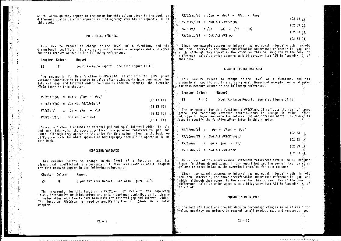
width although they appear in the axiom for this column given in the book on - PRICErep(u) m (Qun — Quo) * (Pun — Puo]difference which appears as bibliography item A15 in Appendix B of (C2 E3this book. . PRICErep(U) SUM ALL PRIrep(u)
(C2 E3PRICErep m (Qn — Qo] * (Pn — Po]
(C2 E3PURE PRICE VARIANCE PRICErep(I) SUN ALL PRIrep
(C2 E3 44)
This measure refers to change in the level of a function, and its Since our example assumes no interval gap and equal interval width in olddimensional coefficient is a currency unit. Numerical examples and a diagram and new intervals, the above specification suppresses reference to gap and
for this measure appear in the following references. width although they appear in the axiom for this column given in the book ondifference calculus which appears as bibliography item A15 in Appendix 4 of
Chapter Column Report this book.
E3 F Input Variance Report. See also Figure E3.F3ADJUSTED PRICE VARIANCE
The mneumonic for this function is PRICEo7d. It reflects the pure pricevariance contribution to change in value after adjustments have been made for This measure to change in the level of a function, and itsinterval gap and interval width. PRICEo1d is used to specify the function dimensional coefficient is a currency unit. Numerical examples and aAVoid later in this chapter. for this measure appear in the following references.
Chapter Column 'ReportPRICEo1d(u) a Quo * (Pun — Puo]
(C2 E3 Fl) E3 F + C Input Variance Report. See also Figure E3.F5PRICEo1d(U) a SUM ALL PRICEoJd(u)
(C2 E3 F2)PRICEo7d a Qo * (Pn — Po] The mneumonic for this function is PRICEneW. It reflects the sum of uure
(C2 E3 F3) price and repricing variance contributions to change in valuePRICEoJd(I) a SUM ALL PRICEo1d adjustments have beet made for interval gap and interval width. PRICEnety" is
(C2 E3 F4) used to specify the function IsPnew later in this chapter.
Since our example assumes no interval gap and equal interval width in old -
and new intervals, the above specification suppresses reference to gap and PRICEneW(u) m Qun * (Pun — Puo]
width although they appear in the axiom for this column given in the book on (C? E3 Ii)difference calculus which appears as bibliography item A15 jn Appendix B of PRICEnew(U) a SUM ALL PRICEnew(u) -
this book. (C? E3 Hg)PRICEnew a Qn * (Pn — Po]
(C? E3
REPRICING VARIANCE PRICEnew(I) a SUM ALL PRICEnew(C? £3 U4)
This measure refers to change in the level of a function, and its Below each of the above axioms, statement references cite Hi to H4dimensional coefficient is a currency unit. Numerical examples and a diagram these functions do not appear in any report but are the sum of two existingfor this measure appear in the following references. columns as cited below in the numerical examples for this measure.
Chapter Column Report Since our example assumes no interval gap and equal interval width in' oldand new intervals, the above specification suppresses reference to gap and
£3 C Input Variance Report. See also Figure E3.F4 width although they appear in the axiom for this column given in the book ondifference calculus which appears as bibliography item A15 in Appendix U ofthis book.
The mneumonic for this function is PRICErep. It reflects the repricing(i.e., interactive or joint volume and price) variance contribution to changein value after adjustments have been made for interval gap and interval width. CHANGE IN RELATIVES
The function PRICErep is used to specify the function APnew in a laterchapter.
The next six functions provide data on percentage changes in relatives forvalue, quantity and price with respect to all product made and resources
C2—g C2—1O
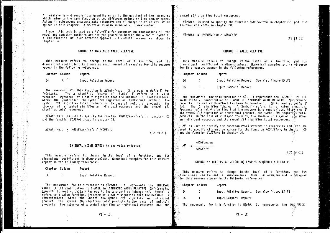
A relative is a dimensionless which is the quotient of two measureswhich refer to the same function at two different points in time and/or space.Axioms in subsequent chapters make extensive use of change in relatives whichappear in this chapter. A relative is also known as an index number.
Since this book is used as a help—file for computer implementations of themodel and computer monitors are not yet geared to handle the A and A symbols,a modification of such notation appears on a computer screen as shown inchapter E4.
CHANGE In INTRINSIC VALUE RELATIVE
This measure refers to change in the level of a function, and itsdimensional coefficient is dimensionless. Numerical examples for this measureappear in the following references.
Chapter Column Report
E4 A Input Relative Report
The mneumonic for this function is Afiintrinsic. It is read as delta V hatintrinsic. The A signifies "change in". Symbol V refers to a valuefunction. Presence of a hat A signifies that the measure is dimensionless.After the j7intrinsic the symbol (u) signifies an individual product, thesymbol (U) signifies total products in the case of multiple products, theabsence of a symbol signifies an individual resource and the symbol (I)signifies total resources.
Atjintrinsic is used to specify the function PROFlTintrinsic in chapter C7
and the function COSTintrinsic in chapter C8.
This measure refers to change in the level of a function, and itsdimensional coefficient is dimensionless. Numerical examples for this measureappear in the following references.
Chapter Column Report
E4 B Input Relative Report
The mneumonic for this function is Aj7width. It represents the INTERVALWIDTH EFFECT contribution to CHANGE in INTRINSIC VALUE RELATIVE Ai7intrinsic.At/width is read as delta V hat width. The A signifies "change in". Symbol V
refers to a value function. Presence of a hat A signifies that the measure isdimensionless. After the Vwidth the symbol (u) signifies an individualproduct, the symbol (U) signifies total products in the case of multipleproducts, the absence of a symbol signifies an individual resource and the
CHANGE In VALUE RELATIVE
This measure refers to change in the level of a function, itsdimensional coefficient is dimensionless. Numerical examples and a :diagramfor this measure appear in the following references.
Chapter Column Report
E4 C Input Relative Report. See also Figure E4.F1
ES H Input Compact Report
The mneumonic for this function is Ajl. It represents the CHANGE IN THEVALUE RELATIVE contribution to CHANGE in INTRINSIC VALUE RELATIVE Aiule,trinsiconce the interval width effect has been factored out. Aji is read as V
hat. The A signifies "change in". Symbol V refers to a value tunction.Presence of a hat A signifies that the measure is dimensionless. Afteb the Vthe symbol (u) signifies an individual product, the symbol (U) signiftps totalproducts in the case of multiple products, the absence of a symbol iigniflesan individual resource and the symbol (I) signifies total resources. 1'
AV is used to the function PROFlTrevenue in chapter C7 and can beused to specify alternative axioms for the function PROFIT1ong in ch4pter C5
and the function COSTlong in chapter C6.
At/ m
VALUEo ld(C2 Cl)
CHANGE Ii (OLD-PRICE-WEIGHTED) LASPEYRES QUANTITY RELATIVE
This measure refers to change in the level of a function, itsdimensional coefficient is dimensionless. Numerical examples and a
for this measure appear in the following references.
Chapter Column Report
E4 D Input Rdlative Report. See also Figure E4.F2
I Input Compact Report
The mneumonic for this function is 14o7d. It represents the
C2 — 11. C2 — 12
symbol (I) signifies total resources.
At/width is used to specify the function PROFITwidth in chapter C7 pnd thefunction COSTwidth in chapter CS.
At/width a VALUEwidth / VALUEoJd(C2 51)
I
At/intrinsic a VALUEintrinsic / VALUEoJd
INTERVAL WIDTH EFFECT In the value relative
(C2 E4 Al)
VALUEchange
E5
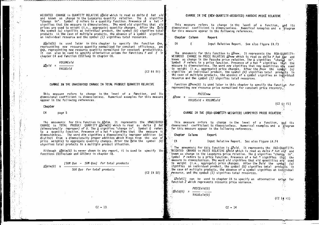
WEIGHTED CHANGE in QUANTITY RELATIVE i4old which is read as delta Q hat oldand known as change in the Laspeyres quantity relative. The A signifies"change in". Symbol Q refers to a quantity function. Presence of a hatsignifies that the measure is dimensionless. The word old signifies that oldprices are used to weight (i.e., aggregate) quantity changes. After thethe symbol (u) signifies an individual product, the symbol (U) signifies totalproducts in the case of multiple products, the absence of a symbol signifiesan individual resource and the symbol (I) signifies total resources.
is used later in this chapter to specify the function Qne,representing new resource quantity normalized for constant efficiency, aedQnp, representing new resource quantity normalized for constant productivity.It can also be used to specify alternative axioms for functions Y and E inchapter C4 and function COSTlong in chapter C6.
VOLUMEo lda
VALUEo Id(C2 E4 Dl)
CHANGE IN THE UNWEIGHTED CHANGE IN TOTAL PRODUCT QUANTITY RELATIVE
This measure refers to change in the level of a function, and itsdimensional coefficient is dimensionless. Numerical examples for this measureappear in the following references.
Chapter
E4 page 5
The mneumonic for this function is It represents the UNWEIGHTED
CHANGE in TDTAL PRDDUCT QUANTITY which is read as delta Q hat(dimensionally improper) of U. The A signifies "change in". Symbol Q refersto a quantity function. Presence of a hat A signifies that the measure isdimensionless. The word dim signifies a dimensionally improper addition (as
distinct from a dimensionally proper addition which flows from the use ofprice weights) to aggregate quantity changes. After the the symbol (U)signifies total products in a multiple product situation.
Although is never shown in any report, it is used to specify thefunctions COSTvolume and COSTmix in chapter C8.
CHANGE IN THE (NEW-QUANTITY-WEIGHTED) PAASCHE PRICE RELATIVE
This measure refers to change in the level of a function, itsdimensional coefficient is dimensionless. Numerical examples and a
for this measure appear in the following references.
Chapter Column Report
E4 E Input Relative Report. See also Figure E4.F3
The mneumonic for this function is It represents the NEW—QUANTITY—WEIGHTED CHANGE in PRICE RELATIVE which is read as delta P hat diw andkeown as change in the Paasche price relative. The A signifies in".Symbol P refersto a price function. Presence of a hat A signifies themeasure is dimensionless. The word new signifies that new quantities usedto weight (i.e., aggregate) price changes. After the Pnew the (u)signifies an individual product, the symbol (U) signifies total prodwts inthe case of multiple products, the absence of a symbol signifies an individualresource and the symbol (I) signifies total resources.
Function LtPnew(U) is used later in this chapter to specify the Pnrrepresenting new resource price normalized for constant price
APnew a
(C2 f4 El)
CHANGE IN THE (OLD-QUANTITY-WEIGHTED) LASPEVRES PRICE RELATIVE
This measure refers to change in the level of a function, abd itsdimensional coefficient is dimensionless. Numerical examples and a
for this measure appear in the following references. -
Chapter Column Report
F Input Relative Report. See also Figure E4.F4
The mneumonic for this function is Sold. It represents the OLD—QUANTITY—WEIGHTED CHANGE in PRICE RELATIVE /sPold which is read as delta P hat ai4 andknown as change in the Laspeyres price relative. The A signifies "changp in".Symbol P refers to a price function. Presence of a hat A signifies tim themeasure is dimensionless. The word old signifies that old quantities er-a- usedte weight (i.e., price changes. After the Pold the (u)signifies an individual product, the symbol (U) signifies total inthe case of multiple products, the absence of a symbol signifies an indfjtidualPesource, and the symbol (I) signifies total resources. -
APold(I) can be used in chapter C6 to specify an alternative forfunction Z which represents resource price variance. -
PRICEo ld(U)A?old(U) a
___________
VALUE0Id(U)
A-.
PRICEnew
VALUEo1d ÷ VOLUMEo1d
a
E4
[SUM Qun — SUM Quo] for total products
(C2 E4 D2)SUM Quo for total products
C? — 14
(C2 E4 El)
J
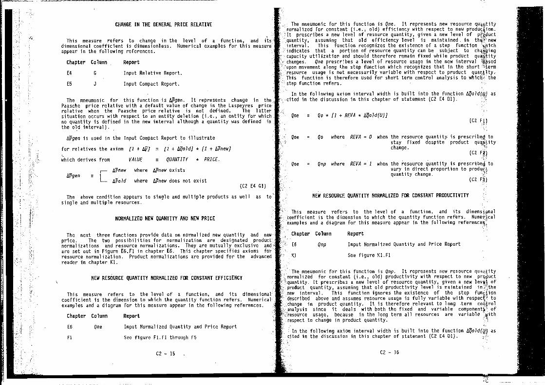
&i__
CHANGE IN THE GENERAL PRICE RELATIVE The mneumonic for this function is Qne. It represents new resource quantitynormalized for constant (i.e., old) efficiency with respect to new production.It prescribes a new level of resource quantity, given a new level of pfdduct
This measure refers to change in the level of a function, and its - quantity, assuming that old efficiency level is maintained in newdimensional coefficient is dimensionless. Numerical examples for this measure interval. This function recognizes the existence of a step functionappear in the following references. indicates that a portion of resource quantity can be subject to
capacity utilization and should therefore remain fixed while productChapter Column Report changes. Qne prescribes a level of resource usage in the new interval Ipsed
upon movement along the step function which recognizes that in the shortE4 G Input Relative Report. resource usage is nut necessarily variable with respect to product
This function is therefore used for short term control analysis to£5 J Input Compact Report. step function refers.
In the following axiom interval width is built into the function as
The mneumonic for this function is It represents change in the cited in the discussion in this chapter of statement (C2 E4 Dl).Paasche price relative with a default value of change in the Laspeyres pricerelative when the Paasche price relative is not defined. The lattersituation occurs with respect to an entity deletion (i.e., an entity for which Qne a Qo * [1 + REVA * AQold(1J)]no quantity is defined in the new interval although a quantity was defined in (C2 F))the old interval).
£Pgen is used in the Input Compact Report to illustrate Qne = Qo where REVA = 0 when the resource quantity is prescribes tostay fixed despite product
for relatives the axiom (1 + IsV.) m (1 ÷ * [1 + APnewJ change.- (C2 II)
which derives from VALUE a QUANTITY * PRICE.Qne = Qnp where REVA = 1 when the resource quantity is prescribed to
i— where IsPnew exists vary in direct proportion toAPgen a quantity change.
L__. LPo7d where NPnew does not exist (C2 fl)(C2 £4 Cl) -
The above condition appears to single and multiple products as well as to NEW RESOURCr QUANTITY NORMALIZED FOR CONSTANT PRODUCTIVITY
single and multiple resources.
This measure refers to the level of a function, and itsNORMALIZED NEW QUANTITY AND NEW PRICE coefficient is the dimension to which the quantity function refers.
examples and a diagram for this measure appear in the following referencea,
The next three functions provide data on normalized new quantity and new Chapter Column Reportprice. The two possibilities for normalization are designated productnormalizations and resource normalizations. They are mutually exclusive and - E6 Qnp Input Normalized quantity and Price Reportare set out in Figure E6.Fl in chapter £6. This chapter specifies axioms forresource normalization. Product normalizations are provided for the advanced Ki See figure K1.Flreader in chapter KI.
The mneumonic for this function is Qnp. It represents new resourceNEW RESOURCE QUANTITY NORMALIZED FOR CONSTANT EFFICIENCY normalized for constant (i.e., old) productivity with respect to new prutjuct
quantity. It prescribes a new level of resource quantity, given a new leve' ofproduct quantity, assuming that old productivity level is maintained in
the level of a function, and its dimensional new interval. This function ignores the existence of the step func$Joncoefficient is the dimension to which the quantity function refers. Numerical described above and assumes resource usage is fully variable with respecU toexamples and a diagram for this measure appear in the following references, change in product quantity. It is therefore relevant to long -term
analysis since it deals with both the fixed and variable ofChapter Column Report resource usage, because in the long term all resources are variable with
respect to change in product quantity.E6 Qne Input Normalized Quantity and Price Report
In the following axiom interval width is built into the function tsQold(Vj asFl See figure Fl.F1 through F5 cited in the discussion in this chapter of statement (C2 E4 Dl).
C2-15 C2-16
j
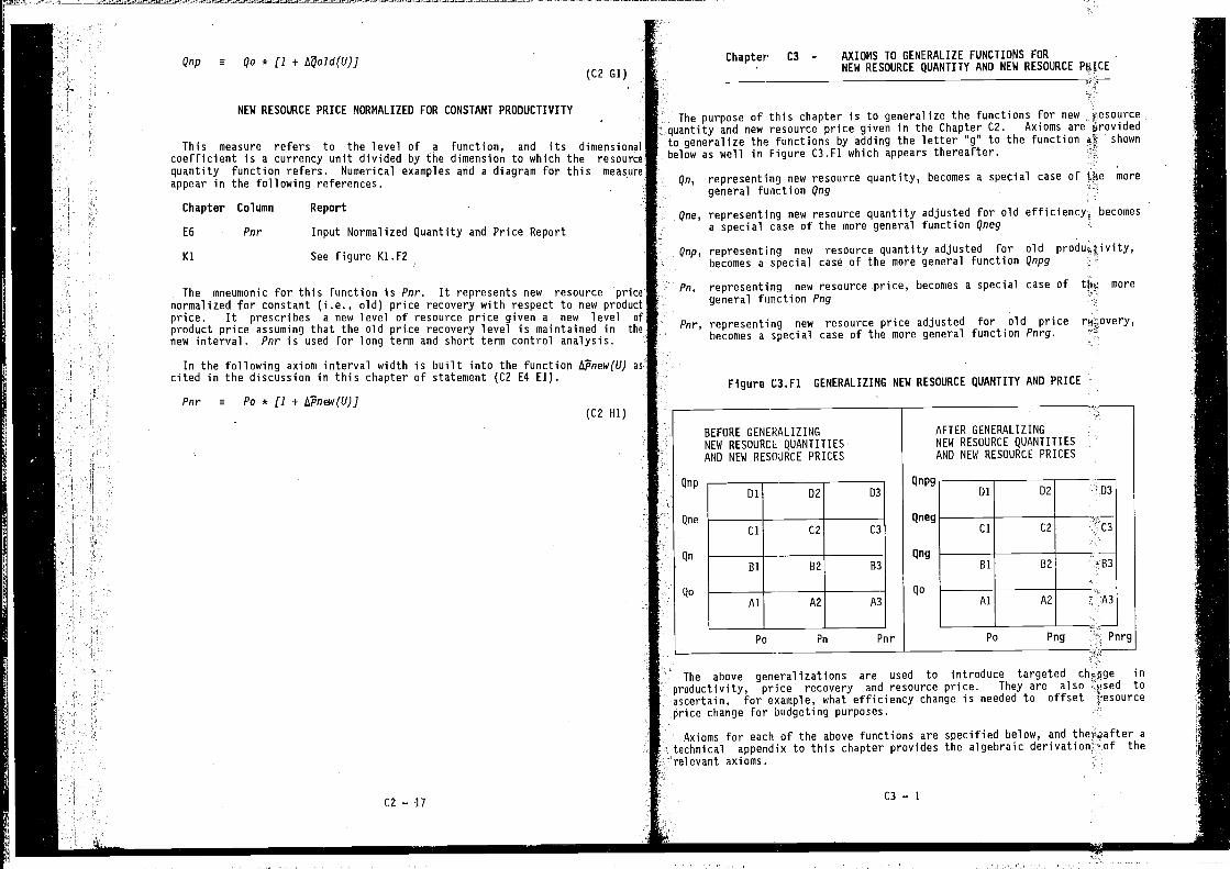
This measure refers to the level of a function, and its dimensionalcoefficient is a currency unit divided by the dimension to which the resourcequantity function refers. Numerical examples and a diagram for this measureappear in the following references.
Chapter Column Report
E6 Par Input Normalized Quantity and Price Report
KI See figure Ki.F2
The mneumonic for this function is Par. It represents new resource pricenormalized for constant (i.e., old) price recovery with respect to new productprice. It prescribes a new level of resource price given a new level ofproduct price assuming that the old price recovery level is maintained in thenew interval. Par is used for long term and short term control analysis.
In the following axiom interval width is built into the function Li2new(U) ascited in the discussion in this chapter of statement (C2 E4 El).
Par m Po * [1 + APaew(U)J(C2 Hi)
Chapter C3 - AXIOMS TO GENERALIZE FUNCTIONS FORNEW RESOURCE QUANTITY ANO NEW RESOURCE PiHCE
The purpose of this chapter is to generalize the functions for new resourcequantity and new resource price given in the Chapter C2. Axioms areto generalize the functions by adding the letter "g" to the function shown
below as well in Figure C3.Fi which appears thereafter.
qa, representing new resource quantity, becomes a special case of the more
general function Qag
Qne, representing new resource quantity adjusted for old efficiency, becomesa special case of the more general function Qaeg
Qap, representing new resource quantity adjusted for old produc4ivity,becomes a special case of the more general function Qapg
Pa, representing new resource price, becomes a special case of tk moregeneral function Png
Par, representing new resource price adjusted for old pricebecomes a special case of the more general function Parg.
Di 02
-
03
Cl
Bl
C2
B2
C3
B3
Al A2 A3
flnnrr
Dl D2
—.—--------—
RI B2
Al A2 A3
Po Pnrg
The above generalizations are used to introduce targeted inproductivity, price recovery and resource price. They are also toascertain, for example, what efficiency change is needed to offset ?esourceprice change for budgeting purposes.
Axioms for each of the above functions are specified below, and thereafter aappendix to this chapter provides the algebraic derivation of the
relevant axioms.
C3 — 1
Qap e Qo * (I + I4old(U)J
NEW RESOURCE PRICE NORMALIZED FOR CONSTANT PRODUCTIVITY
(C2 Gl)4..
C2—17
Figure C3.F1 GENERALIZING NEW RESOURCE QUANTITY AND PRICE
BEFORE GENERALIZINGNEW RESOURCE QUANTITIESAND NEW RESOURCE PRICES
AFTER GENERALIZINGNEW RESOURCE QUANTITIESAND NEW RESOURCE PRICES
Qnp
Qne
Qn
Qo
Cl C2 C3
Qng
Qo
Po Pn Pnr
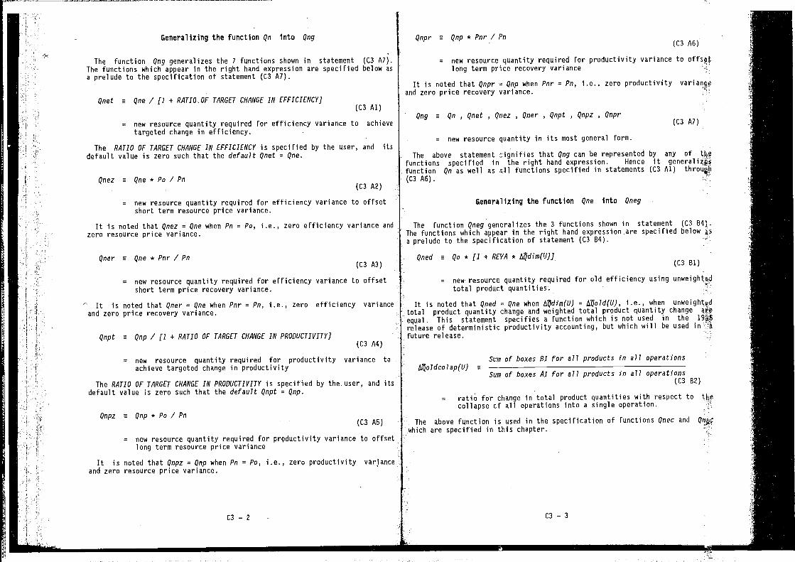
Generalizing the function Qn into Qng
The function Qng generalizes the 7 functions shown in statement (C3 A7).The functions which appear in the right hand expression are specified below asa prelude to the specification of statement (0 A7).
Qnet a Qne / (1 + TARGET CHANGE IN EFFICIENCY](C3 Al)
= new resource quantity required for efficiency variance to achievetargeted change in efficiency.
The RATIO OF TARGET CHANGE IN EFFICIENCY is specified by the user, and itsdefault value is zero such that the default Qnet = Qne.
Qnez a Qne*Po/Pn(C3 A2)
= new resource quantity required for efficiency variance to offsetshort term resource price variance.
It is noted that Qnez = Qne when Pn = Po, i.e., zero efficiency variance andzero resource price variance.
Qner a Qne * Pnr / Pp(C3 A3)
= new resource quantity required for efficiency variance to offsetshort term price recovery variance.
It is noted that Qner = Qne when Pnr = Pn, i.e., zero efficiency varianceand zero price recovery variance.
Qnpt a Qnp / (1 + RATIO OF TARGET CHANGE IN PRODUCTIVITY](C3 A4)
= new resource quantity required for productivity variance toachieve targeted change in productivity
The RATIO OF TARGET CHANGE IN PRODUCTIVITY is specified by the user, and itsdefault value is zero such that the default Qnpt = Qnp.
Qnpz a Qnp*Po/Pn(C3 A5)
= new resource quantity required for prQductivity variance to Offsetlong term resource price variance
It is noted that Qnpz = Qnp when Pn = Po, i.e., zero productivity varianceand zero resource price variance.
Generalizing the function Qne Into Qneg
The function Qneg generalizes the 3 functions shown in statement (C3 B4}.The functions which appear in the right hand expression are specified belowa prelude to the specification of statement (C3 B4).
Qned e Qo * [1 + REVA *(C3 Dl)
= new resource quantity required for old efficiency usingtotal product
It is noted that Qned = Qne when = /4old(U), i.e., whentotal product quantity change and weighted total product quantity change
a function which is not used in the 19DBrelease of deterministic productivity accounting, but which wiU be used in:afuture release.
Sum of boxes Dl for all products in all operations
Sum of boxes Al for all products in all operations(0 B2)
= ratio for change in total product quantities with respect tocollapse cf all operations into a single operation.
The above function is used in the specification of functions Qnec and Qnpc
which are specified in this chapter.
C3—2 C3—3
Qnpr a Qnp * Pnr / Pn(C3 A6)
= new resource quantity required for productivity variance to offsetlong term price recovery variance
It is noted that Qnpr = Qnp when Pnr = Pn, i.e., zero productivityand zero price recovery variance.
Qng e Qn , Qnet , Qnez , Qner , Qnpt , Qnpz , Qnpr(C3 A7)
= new resource quantity in its most general form.
The above statement zignifies that Qng can •be represented by any of thefunctions specified in the right hand expression. Hence it generalizpsfunction Qn as well as functions specified in statements (C3 Al)(C3 A6).
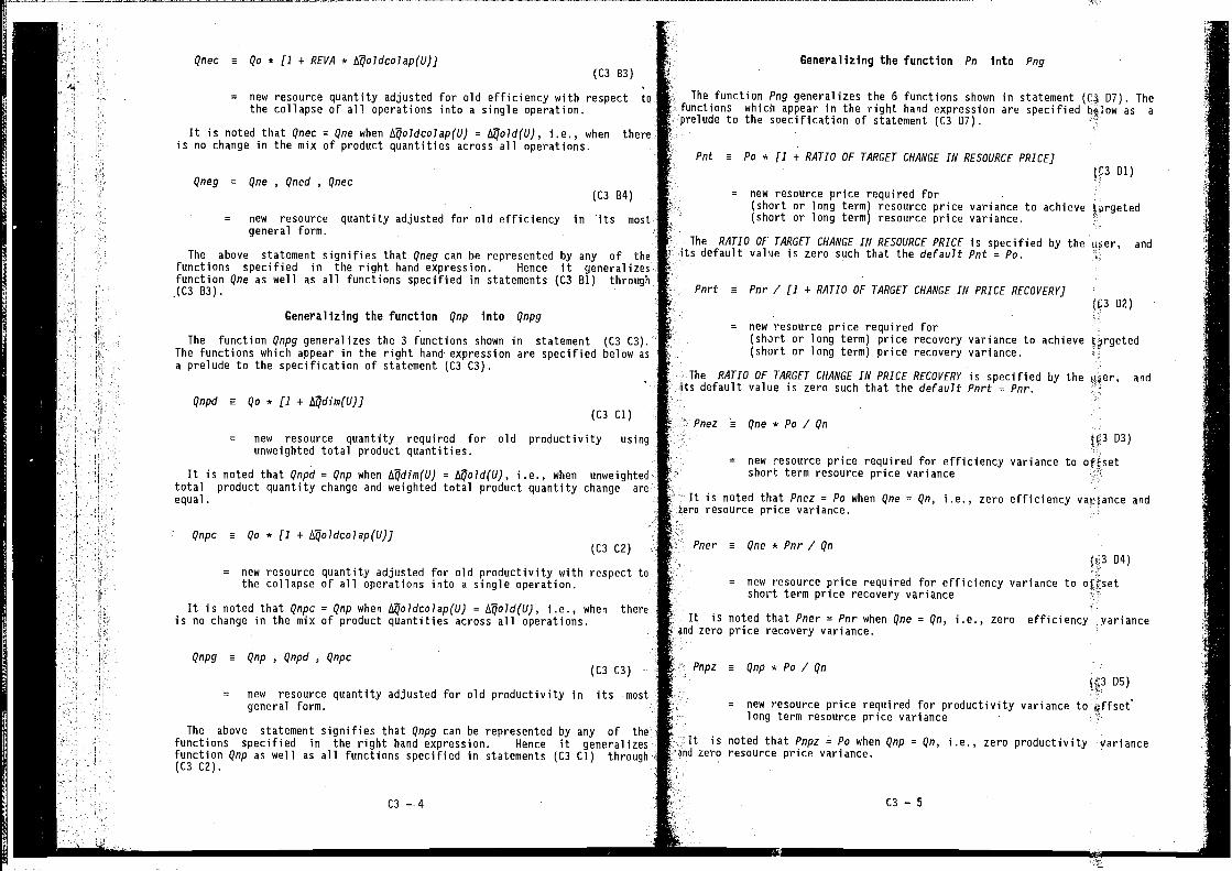
______________________________________- .-
Qnec m Oa * (1 + REVA * liQo7dcalap(U)](C3 83)
= new resource quantity adjusted for old efficiency with respect tethe collapse of all operations into a single operation.
It is noted that Qnec = One when I4aldcalap(U) = i.e., when thereis no change in the mix of product quantities across all operations.
Oneg = Qne , Qned , Qnec(C3 84)
= new resource quantity adjusted for old efficiency in •its mostgeneral form.
The above statement signifies that Qneg can be represented by any of thefunctions specified in the right hand expression. Hence it generalizesfunction One as well as all functions specified in statements (C3 81) through(C3 B3).
Generalizing the function Qnp into Qnpg
The function Qnpg generalizes the 3 functions shown in statement (C3 C3).The functions which appear in the right hand expression are specified below asa prelude to the specification of statement (C3 C3).
Qnpd a 00 * [1 +(C3 Cl)
= new resource quantity required for old productivity usingunweighted total product quantities.
It is noted that Qnpd = Qnp when = i.e., when unweightedtotal product quantity change and weighted total product quantity change areequal
Qnpc m Qo * [1 +(C3 C2)
= new resource quantity adjusted for old productivity with respect tethe collapse of all operations into a single operation.
It is noted that Qnpc = Qnp when t4oldco!ap(U) = i.e., when thereis no change in the mix of product quantities across all operations.
Qnpg a Qnp , Qnpd , Qnpc(C3 C3)
= new resource quantity adjusted for old productivity in its mostgeneral form.
The above statement signifies that Qnpg can be represented by any of thefunctions specified in the right hand expression. Hence it generalizesfunction Qnp as well as all functions specified in statements (C3 Cl) through(C3 C2).
Generalizing the function Pn into Png
The function Png generalizes the 6 functions shown in statement D7). Thefunctions which appear in the right hand expression are specified b*low as aprelude to the specification of statement (C3 D7).
Pnt a Pa * (1 + RATIO OF TARGET CHANGE IN RESOURCE PRICE](C3 01)
= new resource price required for(short or long term) resource price variance to achieve targeted(short or long term) resource price variance.
The RATIO OF TARGET CHANGE IN RESOURCE PRICE is specified by the &4er, andits default vaNe is zero such that the default Pnt = Pa.
Pnrt m Pnr / [1 + RATIO OF TARGET CHANGE IN PRICE RECOVERY](C3 D2)
= new resource price required for(short or long term) price recovery variance to achieve targeted(short or long term) price recovery variance.
The RATIO OF TARGET CHANGE IN PRICE RECOVERY is specified by the andits default value is zero such that the default Pnrt = Pnr.
Pnez One*Po/On03)
= new resource price required for efficiency variance to oftsetshort term resource price variance
It is noted that Pnez = Pa when One = On, i.e., zero efficiency variance andzero resource price variance.
Pner a One * Pnr / On04)
= new resource price required for efficiency variance to offsetshort term price recovery variance
It is noted that Pner = Pnr when One = On, i.e., zero efficiency varianceand zero price recovery variance.
Pnpz a Onp * Pa / OnD5)
= new resource price required for productivity variancelong term resource price variance
It is noted that Pnpz = Pa when Qnp = Qn, i.e., zero productivity varianceand zer? resource price variance.
C3—4 C3—5
H
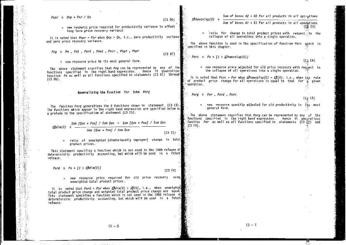
Pnpr a Qnp * Pnr / Qn(C3 06)
= new resource price required for productivity variance to offsetlong term price recovery variance
It is noted that Pnpr = Pnr when Qnp = Qn, i.e., zero productivity varianceand zero price recovery variance.
Png m Pn , Pnt , Pnrt , Pnez , Pner , Pnpz , Pnpr(C3 07)
= new resource price in its most general form.
The above statement signifies that Png can be represented by any of the
functions specified in the right hand expression. Hence it generalizesfunction Pn as well as all functions specified in statements (C3 Dl) through
(C3 06).
Generalizing the function Pnr Into Pnrg
The function Pnrg generalizes the 3 functions shown in statement (C3 ES).The functions which appear in the right hand expression are specified below asa prelude to the specification of statement (C3 ES).
Sum (Qun * Pun] / Sum Qun — Sum (Quo * Puo] / Sum Quoe
Sum (Quo * PuoJ / Sum Quo(C3 El)
= ratio of unweighted (dimensionally improper) change in totalproduct prices.
This statement specifies a function which is not used in the 1988 release efdeterministic productivity accounting, but which will be used in a future
release.
Pnrd a Pa * (1 + tsfidim(U)](C3 E2)
= new resource price required for old price recovery using
unweighted total product prices.
It is noted that Pnrd = Pnr when Ispdim(U) = i.e., when unweightedtotal product price change and weighted total product price change are equal
This statement specifies a function which is not used in the 1988 release at
deterministic productivity accounting, but which will be used in a future
release.
C3—-6
Sum of boxes A2 + 82 for all products in a77 operAtionsIsPnewcolap(U) a
Sum of boxes Al + Bl for all products in all operationsE3)
= ratio for change in total product prices with respect to thecollapse of all operations into a single operation.
The above function is used in the specification of function Pnrc which isspecified in this chapter. if
Pnrc a Po * (1 + bPnewcolap(U)]E4)
= new resource price adjusted for old price recovery with tothe collapse of all operations into a single operation. '
It is noted that Pnrc = Pnr when /sPnewcolap(U) = i.e., when tine rateof product price change for all operations is equal to that for 4' givenoperation.
Pnrg a Pnr , Pnrd , Pnrc(Q,i E5)
= new resource quantity adjusted for old productivity in Rn most• general form.
The above statement signifies that Pnrg can be represented by any pf thefunctions specified in the right hand expression. Hence itfunction Pnr as well as all functions specified in statements (C3 fl) and(13 E4). if
-i
13 — 7
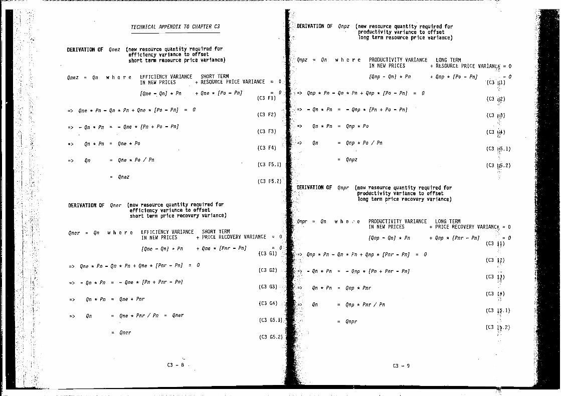
Qaez (new resource quantity required forefficiency variance to offsetshort term resource price variance)
e r e EFFICIENCY VARIANCE SHORT TERM
IN NEW PRICES + RESOURCE PRICE VARIANCE
[Qne—Qa]*Pa +Qae*(Po—Pa](C3
_Qn*Pa+Qae*[Po—Pa] = 0(C3
= — Qae * [Pa + Po — Pa](C3
= Qae * Po(C3
= Qae*Po/Pa
= Qaez
Qaer (new resource quantity required forefficiency variance to offsetshort term price recovery variance)
e r e EFFICIENCY VARIANCE SHORT TERM
IN NEW PRICES + PRICE RECOVERY VARIANCE = 0
[Qae—Qa] *Pa +Qae* [Par—Pa] = 0
(C3 Gl)
*Pa+Qae* [Par—Pa] = 0(C3 G2)
— Qae * [Pa + Par — Pa](C3 G3)
= Qae * Par(C3 G4)
= Qae*Par/Pa = Qaer(C3 G5.l)
= Qaer(C3 G5.2)
w h e r e PROOUCTIVITY VARIANCE LONG TERMIN NEW PRICES + RESOURCE PRICE = 0
[Qap—Qa]*Pa +Qap*(Po—Pa] =0(C3 111)
Qa*Pn+Qap*[Po—Pa] = 0(C3
= —Qap*[Pa+Po—Pa](C3
= Qnp*Po(C3 U4)
= Qap*Po/Pa(C3
= Qapz(C3
Qapr (new resource quantity required forproductivity variance to offsetlong term price recovery variance)
w ii e e PROOUCTIVITY VARIANCE LONG TERMIN NEW PRICES + PRICE RECOVERY VARIANC[ = 0
(Qap—Qa]*Pa +Qap*(Par—Pa] =0(C3 fl)
* Pa + Qap * [Par — Pa] = 0
(C3 12)
— Qap * [Pa + Par — Pa](C3 )3)
= Qap * Par(C3 14)
= Qap*Par/Pa(C3
= Qapr(C3
C3—8 C3—9
TECHNICAL APPENDIX TO CHAPTER C3 DERIVATION OF Qapz (new resource quantity required forproductivity variance to offsetlong term resource price variance)
DERIVATION OF
Qaez = Qa wh
=> Qae * Pa
— Qa * Pa
=> Qa*Pa
=> Qa
DERIVATION OF
=0=0
Fl)
F2)
F3)
F4)
(C3 F5.1)
(C3 F5.2)
Qapz = Qa
=> Qap * Pa —
a — Qa * Pa
=> Qa*Pa
=> Qa
DERIVATION OF
Qapr = Qa
Qaer = Qa wh
=> Qae * Pa — Qa
— Qa * Pa =
=> Qa*Pa
a Qa
H
a
Qap * Pa — Qa
—Qa*Pa =
Qa * Pa
Qa
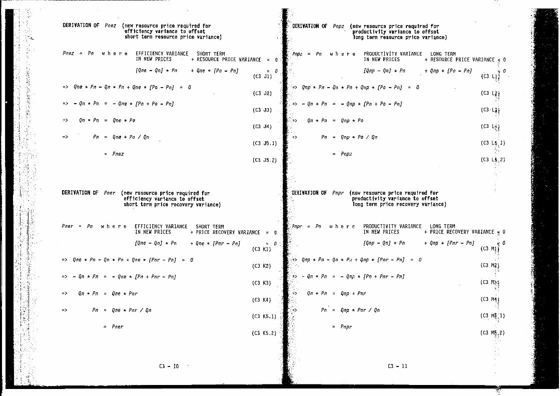
DERIVATION OF Pnez (new resource price required forefficiency variance to offsetshort term resource price variance)
Pnez = Pn w h e r e EFFICIENCY VARIANCE SHORT TERNIN NEW PRICES + RESOURCE PRICE VARIANCE =
[Qne—QnJ*Pn +Qne*(Po.-PnJ = 0
(C3 JI)
=> Qne*Pn—Qn*Pn+Qne*(Po_pn] = 0(C3 J2)
=> —Qn*Pn = —Qne*[Pn+Po—PnJ(C3 J3)
=> Qn*Pn = Qne*Po(C3 J4)
=> - Pn = Qne*Po/Qn(C3 J5.1)
= Pnez(C3 J5.2)
DERIVATION OF Pner (new resource price required forefficiency variance to offsetshort term price recovery variance)
Pner = Pn w h e r e EFFICIENCY VARIANCE SHORT TERMIN NEW PRICES + PRICE RECOVERY VARIANCE = 0
(Qne—QnJ*Pn +Qne*(Pnr—PnJ = 0
(C3 KI)
Qn*Pn+Qne*[Pnr—PnJ = 0
(C3 K2)
= —Qne* (Pn+Pnr—PnJ(C3 K3)
= Qne * Pnr(C3 K4)
= Qne*Pnr/Qn(C3 K5.l)
= Pner(C3 K5.2)
Pnpz (new resource price required forproductivity variance to offsetlong term resource price variance)
w h e r e PROOUCTIVITY VARIANCE LONG TERMIN NEW PRICES + RESOURCE PRICE VARIANCE 0
[Qnp—QnJ*Pn +Qnp*(Po—PnJ(C3
-Qn*Pn+Qnp*(Po—PnJ = 0
(C3 L?1
= —Qnp*[Pn+Po—PnJ(C3-
= Qnp*Po(C3
= Qnp * Po / Qn(C3
= Pnpz(C3
DERIVATION OF Pnpr (new resource price required forproductivity variance to offsetlong term price recovery variance)
a Qnp * Pn —
— Qn * Pp
'=> Qn *Pp
a Pn
w h e r e PROOUCTIVITY VARIANCE LONG TERMIN NEW PRICES + PRICE RECOVERY VARIANCE 0
(Qnp-QnJ*Pn +Qnp*(Pnr-PnJ(C3 Nfl
Qn*Pi-i-Qnp*(Pnr—PnJ = 0(C3 Mfl
= —Qnp*(Pn-i-Pnr—Pnj(C3
= Qnp-kPnr(C3 M4;
= Qnp*Pnr/Qn(C3
= Pnpr(C3
C3—l0 C3—1l
• DERIVATION OF
Pnpz = Pp
r> Qnp * Pp
a - Qn * pp
=> Qp*Pp
a Pp
It
Qne *
— Qn * pp
=>
=>
=>
=>
Pnpr = Pp
Qp * pp
pp
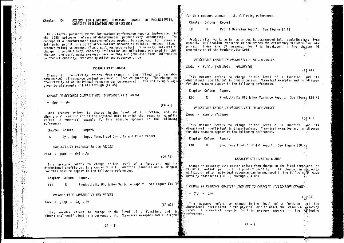
Chapter C4 AXIOMS FOR FUNCTIONS TO MEASURE CHANGE IN PRODUCTIVITY,CAPACITY UTILIZATION AND EFFICIENCY
This chapter presents axioms for various performance reports implemented in
the 1988 software release of determinstic productivity accounting. The
concept of a "performance" measure relates product to resource. For example,intrinsic profit is a performance measure because it relates revenue (i.e.,product value) to expense (i.e., cost resource value). Similarly, measures ofchange in productivity, capacity utilization and efficiency reviewed in thischapter are performance measures because they are generated from informationon product quantity, resource quantity and resource price.
PRODUCTIVITY CHANGE
Change in productivity arises from change in the (fixed and variablecomponents) of resource content per unit of product quantity. The change inproductivity of an individual resource can be measured in the following 5 waysgiven by statements (C4 Al) through (C4 AS).
CHANGE IN RESOURCE QUANTITY OUE TO PRODUCTIVITY CHANGE
= Qnp — Qn(C4 Al)
This measure refers to change in the level of a function, and itsdimensional coefficient is the physical unit to which the resource quantityrefers. A numerical example for this measure appears in the followingreferences.
Chapter Column Report
E6 Qn , Qnp Input Normalized Quantity and Price report
PRODUCTIVITY VARIANCE IN OLD PRICES
Yold = (Qnp — QnJ * Po(C4 A2)
This measure refers to change in the level of a function, and itsdimensional coefficient is a currency unit. Numerical examples and a diagranfor this measure appear in the following references.
Chapter Column Report
£16 B Productivity Old & New Variance Report. See figure E16.F1
PRODUCTIVITY VARIANCE IN NEW PRICES
Ynew = (Qnp — Qn] *(C4 A3)
This measure refers to change in the level of a function, and itsdimensional coefficient is a currency unit. Numerical examples and a diagran
C4 —
1
for this measure appear in the following references.
Chapter Column Report
£9 0 Profit Overview Report. See figure E9.Fl
Productivity variance in new prices is decomposed into contributiqns fromcapacity utilization variance in new prices and efficiency variance in newprices. There are 13 segments for this breakdown in the chapter D3presentation of the Productivity Grid.
PERCENTAGE CHANGE IN PRODUCTIVITY IN OLD PRICES
= Yold / [VALUEo7d + VOLUNE07d](q A4)
This measure refers to change in the level of a function, itsdimensional coefficient is dimensionless. Numerical examples and a
for this measure appear in the following references.
Chapter Column Report
£16 £ Productivity Old & New Variance Report. See figuru El6.F2
PERCENTAGE CRINGE IN PRODUCTIVITY IN NEW PRICES
A7new = Ynew / V'lLUEnew(Cf A5)
This measure refers to change in the level of a function, &nd itsdimensional coefficient is dimensionless. Numerical examples and a diagramfor this measure appear in the following references.
Chapter Column Report
£10 0 Long Term Product Profit Report. See figure
CAPACITY UTILIZATION CHANGE
Change in capacity utilization arises from change in the fixed ofresource content per unit of product quantity. The change inutilization of an individual resource can be measured in the waysgiven by statements (C4 81) through (C4 85).
CHANGE IN RESOURCE QUANTITY USED DUE TO CAPACITY UTILIZATION CHANGE
= Qnp — Qne
(Cf 81)
This measure refers to change in the level of a function, itsdimensional coefficient is the physical unit to which the resourcerefers. A numerical example for this measure appears in the fjllowingreferences. - -'
C4-2
1
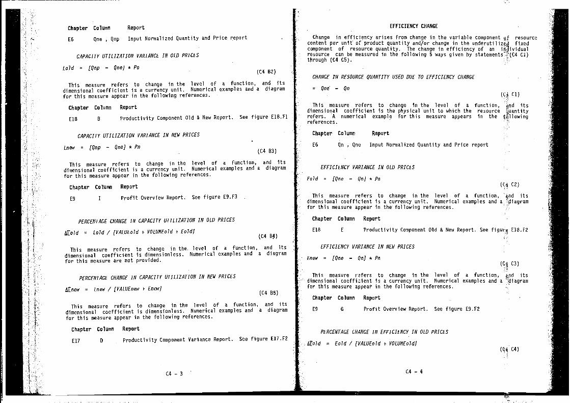
Chapter Column Report EFFICIENCY CHANGE
E6 Qne , Qnp Input Normalized Quantity and Price report Change in efficiency arises from change in the variable component resourcecontent per unit product quantity and/or change in the underutilized fixedcomponent of resource quantity. The change in efficiency of an
CAPACITY UTILIZATION VARIANCE IN OLD PRICES resource can be measured in the following 5 ways given by statements Cl)through (C4 C5).
Lold = [Qnp — QneJ*Po(C4 B2)
CHANGE IN RESOURCE QUANTITY USED DUE TO EFFICIENCY CHANGE
This measure refers to change in the level of a function, and itsdimensional coefficient is a currency unit. Numerical examples and a diagram = Qnd — Qn
for this measure appear in the following references. Cl)
Chapter Column Report This measure refers to change in the level of a function, itsdimensional coefficient is the physical unit to which the resource
E18 B Productivity Component Old & New Report. See figure E18.F1 refers. A numerical example for this measure appears in thereferences.
CAPACITY UTILIZATION VARIANCE IN NEW PRICES Chapter Column Report
Lnew = (Qnp — QneJ * E6 Qn , Qne Input Normalized Quantity and Price report(C4 B3)
This measure refers to change in the level of a function, and itsdimensional coefficient is a currency unit. Numerical examples and a diagram EFFICIENCY VARIANCE IN OLD PRICES
for this measure appear in the following references.Eold = [Qne — QnJ*Po
Chapter Column Report (C$ C2)
E9 I Profit Overview Report. See figure E9.F3 . This measure refers to change in the level of a function, itsH . dimensional coefficient is a currency unit. Numerical examples and a
for this measure appear in the following references. -.
PERCENTAGE CHANGE IN CAPACITY UTILIZATION IN OLD PRICES Chapter Column Report
pAtold = Lold / (VALUE0Jd + VOLUMEo7d + EoJdJ E18 E Productivity Component Old & New Report. See E18.F2
(C48fl
This measure refers to change in the. level of a function, and its EFFICIENCY VARIANCE IN NEW PRICES
dimensional coefficient is dimensionless. Numerical examples and a diagramfor this measure are not provided. Enew = (Qne — QnJ * Pn
C3)
PERCENTAGE CHANGE IN CAPACITY UTILIZATION IN NEW PRICES This measure refers to change in the level of a function, itsdimensional coefficient is a currency unit. Numerical examples and a
Atnew = Lnew / rVALUEOOW + EnewJ for this measure appear in the following references.(C4 B5)
Chapter Column Report
This measure refers to change in the level of a function, and its4 1
dimensional coefficient is dimeAsionless. Numerical examples and a diagram ES 0 Profit Overview Report. See figure E9.F2
Hfor this measure appear in the following references.
Chapter Column ReportPERCENTAGE CHANGE IN EFFICIENCY IN OLD PRICES
U E17 0 Productivity Component Variance Report. See figure E17.F2= Eold / (VALUE0Jd + VOLUMEoIdJ
(Q4 C4)
C4 -3 C4 -4
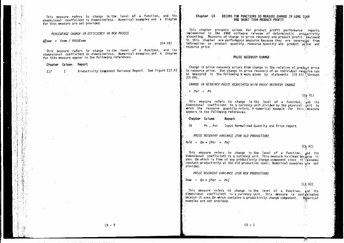
This measure refers to change in the level of a function, and its Chapter CS AXIOMS FOR FUNCTIONS TO NEASURE CHANGE IN LONGdimensional coefficient is dimensionless. Numerical examples and a diagram AND SHORT TERM PRODUCT PROFITfor this measure are not provided.
This chapter presents axioms for product profit performance reportsPERCENTAGE CHANGE IN EFFICIENCY IN NEW PRICES implemented in the 1988 software release of determinstic pro4uctivity
accounting. Measures of change in price recovery and product profitlsrnew = Enew / VALUEnew in this chapter are performance measures because they are from
(C4 CS) information on product quantity, resource quantity and product pj4ce andresource price.
This measure refers to change in the level of a function, and itsdimensional coefficient is dimensionless. Numerical examples and a diagramfor this measure appear in the following references. PRICE RECOVERY CHANGE
Chapter Column Report .
Change in price recovery arises from change in the relation of prodit$ priceE17 E Productivity Component Variance Report. See figure E17.F2 to resource price. The change in price recovery of an individual resdiirce can
be measured in the following 9 ways given by statements (C5 Al)• (C5 AS).
CHANGE IN RESOURCE PRICE ASSOCIATED WITH PRICE RECOVERY CHANGE
= Pnr — Pn
• (Ce: Al)
This measure refers to change in the level of a function, itsdimensional coefficient is a currency unit divided by the physical unit towhich the resource quantity refers. A numerical example for this
in the following references.
Chapter Column Report
E6 Pn , Pnr Input Normalized Quantity and Price report
PRICE RECOVERY VARIANCE (FOR OLD PRODUCTION)
Rold = Qa * [Per —
(c A2)This measure refers to change in the level of a function, its
- dimensional coefficient is a currency unit. This measure is clean itnses Qo which is free of any productivity change component sinceconstant productivity at the old production level. Numerical examples iwe notprovided.
PRICE RECOVERY VARIANCE (FOR NEW PRODUCTION)
Rnew = Qn*[Pnr — Pc]
This measure refers to change in the level of a function, end itsdimensional coefficient is a currency unit. This measure isbecause it uses Qn which contains a productivity change component. Nijjericalexamples are not provided.
C4-5 CS-i
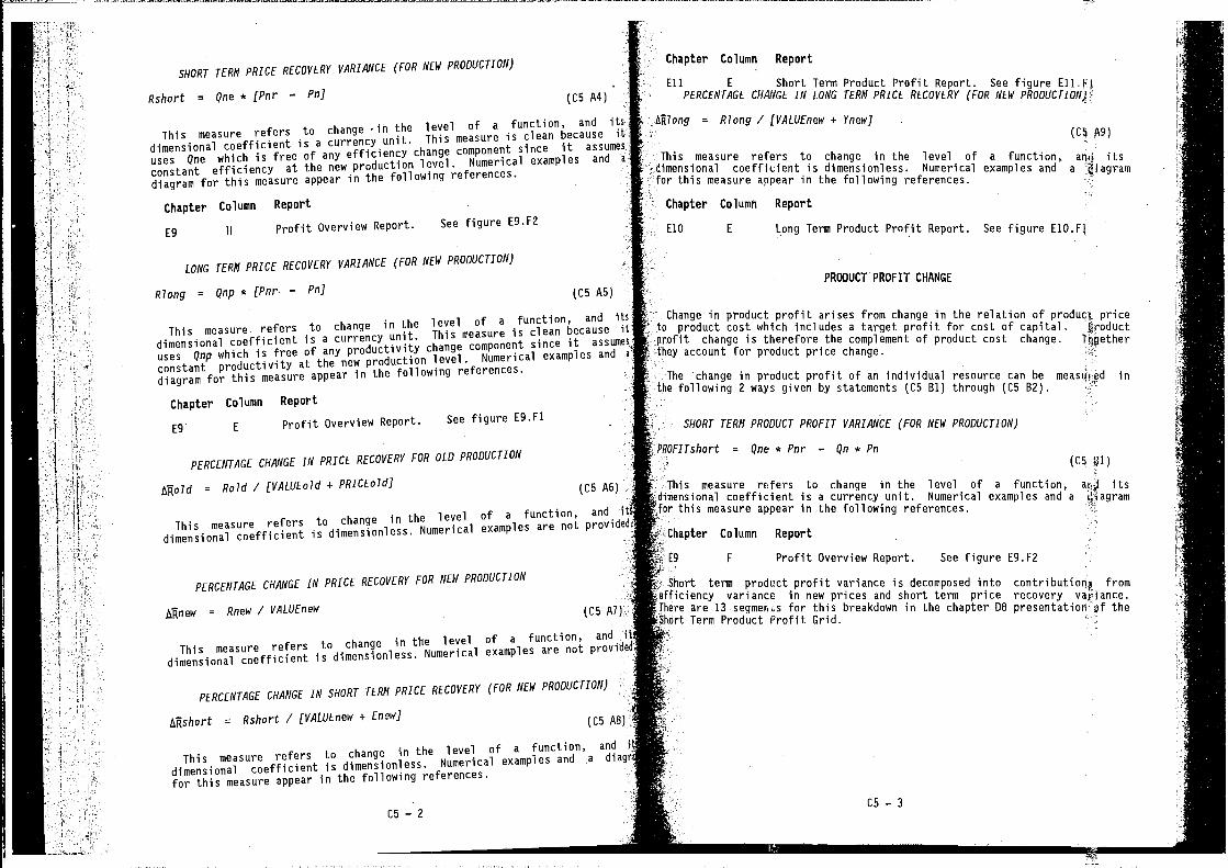
4—
Rshort = Qne * (P1w — PnJ
This measure refers to change •in the level of a function, and itdimensional coefficient is a currency unit. This measure is clean because L
uses Qne which is free of any efficiency change component since it assumes
constant efficiency at the new production level. Numerical examples and a
diagram for this measure appear in the following references.
Chapter Column Report
£9 H Profit Overview Report. See figure E9.F2
LONG TERM PRICE RECOVERYVARIANCE (FOR NEW PRODUCTION)
Riong = Qnp * fPnr — PnJ
This measure refers to change in the level of a function, and I.
dimensional coefficient is a currency unit. This measure is clean because L
uses Qnp which is free of any productivity change component since it assumes
constant productivity at the new production level. Numerical examples and a
diagram for this measure appear in the following references.
Chapter Column Report
E9 EProfit Overview Report. See figure E9.F1
PERCENTAGE CHANGE IN PRICE RECOVERY FOR OLD PRODUCTION
= Rold / [VALUE07d + PRICE0JdI
This measure refers to change in the level of a function, and i
dimensional coefficient is dimensionless. Numerical examples are not provides
PERCENTAGE CHANGE IN PRICE RECOVERY FOR NEW PRODUCTION
= Rnew / VALUEneW
This measure refers to change in the level of a function, and ii,
dimensional coefficient is dimensionless. Numerical examples are not
PERCENTAGE CHANGE IN SHORT TERN PRICE RECOVERY (FOR NEW PRODUCTION) H
CRshort = Rshort / (VALUEneW + Enew]
This measure refers to change in the level of a function, and i
dimensional coefficient is dimensionless. Numerical examples and a dirfor this measure appear in the following references.
C5 — 2
Chapter Column Report
?9)
E1O E Long Term Product Profit Report. See figure E1O.F1
PRODUCT PROFIT CHANGE
Change in product profit arises from change in the relation of product priceto product cost which includes a target profit for cost of capital. •roductprofit change is therefore the complement of product cost change.they account for product price change.
The •change in product profit of an individual resource can be inthe following 2 ways given by statements (CS 81) through (C5 82).
SHORT TERM PRODUCT PROFIT VARIANCE (FOR NEW PRODUCTION)
= Qne * Pnr — Qn *(CS
This measure refers to change in the level of a function,a currency unit. Numerical examples and a diagram
this measure appear in the following references.
sapter Column Report
F Profit Overview Report. See figure E9.F2
iort term product profit variance is decomposed into fromficiency variance in new prices and short term price recoveryere are 13 segmerics for this breakdown in the chapter 08 presentation pf the
Term Product Profit Grid.
CS — 3
SHORT TERN PRICE RECOVERY VARIANCE (FOR NEW PRODUCTION)
(CS A4)Eli E Short Term Product Profit Report. See figure
PERCENTAGE CHANGE IN LONG TERN PRICE RECOVERY (FOR NEW PRODUCTION)
= R7ong / (VALUEnew + Ynew)
This measure refers to change in the level of a function, itsdimensional coefficient is dimensionless. Numerical examples and a jjiagramfor this measure appear in the following references.
Chapter Column Report
(C5 All
(CS A8)
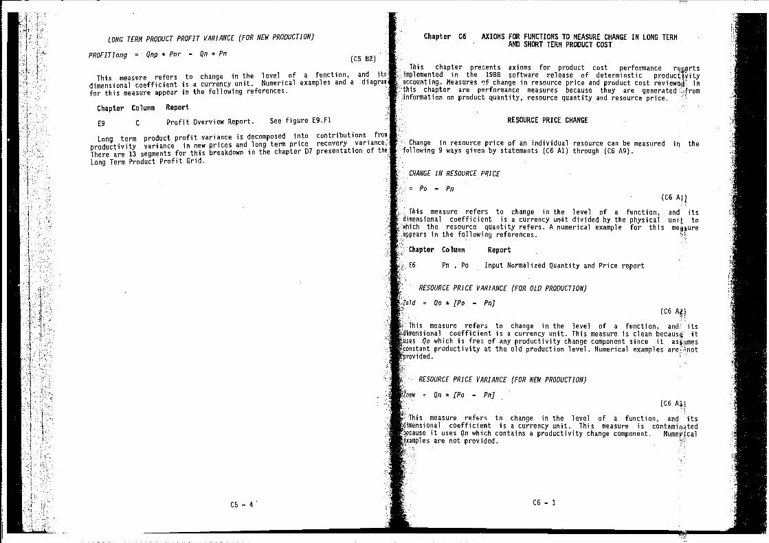
LONG TERM PRODUCT PROFIT VARIANCE (FOR NEW PRODUCTION) Chapter C6 AXIOMS FOR FUNCTIONS TO MEASURE CHANGE IN LONG TERNAND SHORT TERM PRODUCT COST
PROFITPong = Qnp * Pnr — Qn * Pn(CS 82)
This chapter presents axioms for product cost performance reportsThis measure refers to change in the level of a function, and its implemented in the 1988 software release of determinstic
dimensional coefficient is a currency unit. Numerical examples and a diagram -. accounting. Measures 'if change in resource price and product cost infor this measure appear in the following references. this chapter are performance measures because they are generated
information on product quantity, •resource quantity and resource price.Chapter Column Report
E9 C Profit Overview Report. See figure E9.F1 RESOURCE PRICE CHANGE
Long term product profit variance is decomposed into contributions from
productivity variance in new prices and long term price recovery variance. Change in resource price of an individual resource can be measured in theThere are 13 segments for this breakdown in the chapter D7 presentation of the following 9 ways given by statements (C6 Al) through (C6 A9).Long Term Product Profit Grid.
CHANGE IN RESOURCE PRICE
= Po — Pn
(C6 A!)
This measure refers to change in the level of a function and itsdimensional coefficient is a currency un.it divided by the physical unit towhich the resource quantity refers. A numerical example for this meOureappears in the following references.
Chapter Column Report
E6 Pn , Po Input Normalized quantity and Price report
RESOURCE PRICE VARIANCE (FOR OLD PRODUCTION)
laid = Qo * (P0 — Pn](C6
This measure refers to change in the level of a function, and itsdimensional coefficient is a currency unit. This measure is clean ituses Qo which is fre! of any productivity change component since it
productivity at the old production level. Numerical examplesprovided.
RESOURCE PRICE VARIANCE (FOR NEW PRODUCTION)
mew = Qn * (Po — PnJ
(C6A3i
This measure refers to change in the level of a function, and itsdimensional coefficient is a currency unit. This measure is contamits4tedbecause it uses Qn which contains a productivity change component. Numericalexamples are not provided.
C5—4 C6—1

SHORT TERM RESOURCE PRICE VARIANCE (FOR NEW PRODUCTION)
Zshort = Qne * (P0 — Pnj(C6 A4)
This measure refers to change in the level of a function, anddimensional coefficient is a currency unit. This measure is clean because I
uses Qne which is free of any efficiency change component since it assunsconstant efficiency at the new production level. Numerical examples anddiagram for this measure appear in the following references.
Chapter Column Report
E13 H Cost Overview Report. See figure E13.F2
LONG TERM RESOURCE PRICE VARIANCE (FOR NEW PROOUCTION)
Ziong = Qnp * (Po — Pn]
This measure refers to change in the level of a function, and Pdimensional coefficient is a currency unit. This measure is clean becauseuses Qnp which is free of any productivity change component since itconstant productivity at the new production level. Numerical examples anddiagram for this measure appear in the following references.
Chapter Column Report
E13 E Cost Overview Report. See figure E13.F1
PRODUCT COST CHANGE
Change in product cost (which includes a target profit for cost of capitsl)f an individual resource can be measured in the following 2 ways giventatements (C6 Ri) through (C6 B2).
SHORT TERM PRODUCT COST VARIANCE (FOR NEW PRODUCTION)
COSTshort = Qne * Pa — Qn * Pn(C6 Ri)
us measure refers to change in the level of a function, and itsnensional coefficient is a currency unit. Numerical examples and a diagram
this measure appear in the following references.
bct Column Report
E13 F Cost Overview Report. See figure E13.F2
term product cost variance is decomposed into contributions fromiciency variance in new prices and short term resource price
nre are 13 segments for this breakdown in the chapter D5 presentation of (lienrt Term Product Cost Grid.
LONG TERM PROOUCT COST VARIANCE (FOR NEW PRODUCTION)
COSTlong = Qnp * Pa — * Pn(C6 B2)
This measure refers to change in the level of a function, and itswnsional coefficient is a currency unit. Numerical examples and a diagfim
this measure appear in the following references. -:
Column Report
C Cost Overview Report. See figure E13.F1
term product cost variance is decomposed into contributions frqmctivity variance in new prices and long term resource price varianàj.e are 13 segments for this breakdown in the chapter 04 presentation of itue'Term Product Cost Grid.
PERCENTAGE CHANGE IN LONG TERM RESOURCE PRICE (FOR NEW PRODUCTION)
7/ong = — Ziong / (VALUE01d + VOLUMEoJd + Yold](C6
5 measure refers to change in the level of a function, andmensional coefficient is dimensionless. Numerical examples and a diaØamr this measure appear in the following references.
Chapter Column Report
i4 E Long Term Product Cost Report. See figure E14.F1
Attention is drawn to the footnote on the final page of chapter E15.
ii
4
it11
ft
PERCENTAGE CHANGE IN RESOURCE PRICE FOR OLD PRODUCTION
lxYold = — Zo7d / VALUEo7d
This measure refers to change in the level of a function, •anddimensional coefficient is dimensionless. Numerical examples are not provide
PERCENTAGE CHANGE IN RESOURCE PRICE FOR NEW PRODUCTION
A7new = — Znew / (VALUEoJd + VOLUMEoJd]
This measure refers to change in the level of a function, and I'dimensional coefficient is dimensionless. Numerical examples are not
PERCENTAGE CHANGE IN SHORT TERN RESOURCE PRICE (FOR NEW PRODUCTION)
ts7short = — Zshort / (VALUE0Jd + VOLUNEod + Eold](C6 AR)
This measure refers to change in the level of a function, anddimensional coefficient is dimensionless. Numerical examples and a d€for this measure appear in the following references.
Chapter Column ReportE15 E Short Term Product Cost Report. See figure E15.F1
C6 — 2 C6 — 3
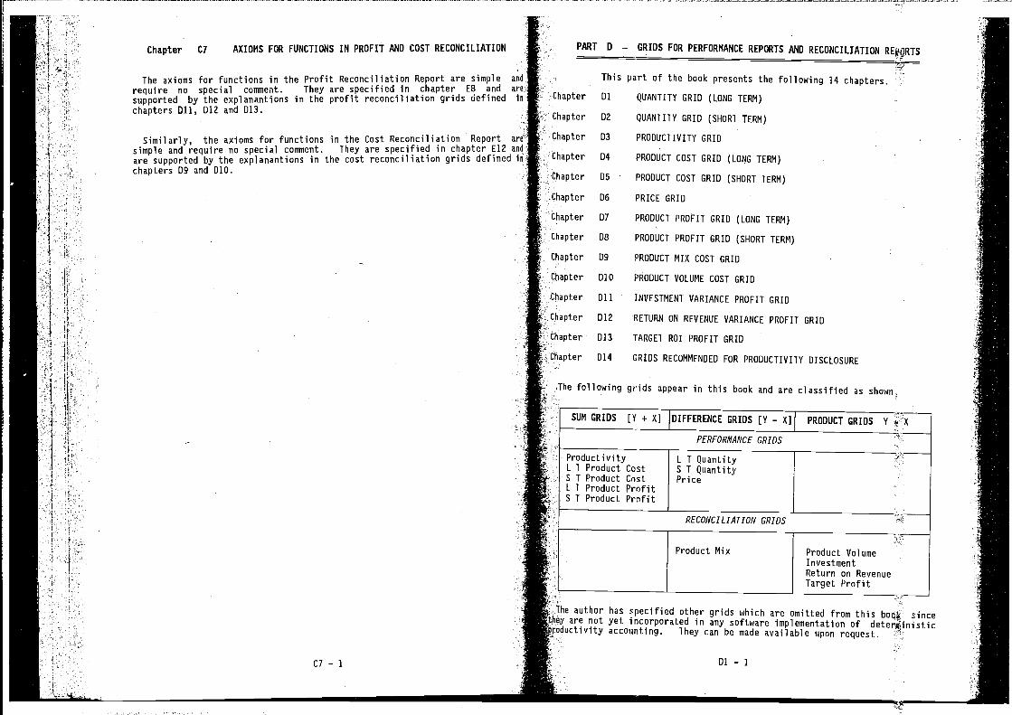
— — — — — — — — — — — — a a' U • ——
AXIOMS FOR FUNCTIONS IN PROFIT AND COST RECONCILIATION PART D — GRIDS FOR PERFORMANCE REPORTS AND RECONCILIATION RERQRTS
This part of the book presents the following 14 chapters.
Chapter D2 QUANTITY GRID
Chapter D3
(SHORT TERM)
PRODUCTIVITY GRID
Chapter D4 PRODUCT COST GRID
Chapter D5
TERM)
PRODUCT COST GRID
Chapter D6
(SHORT TERM)
PRICE GRID
Chapter
Chapter
D7
D8
PRODUCT PROFIT GRID (LONG TERM)
PRODUCT PROFIT GRID
Chapter D9
(SHORT TERM)
PRODUCT MIX COST GRID
Chapter 010 PRODUCT VOLUME COST GRID
Chapter
Chapter
D1I
D12
INVESTMENT VARIANCE PROFIT GRID
RETURN ON REVENUE VARIANCE
D13
PROFIT
TARGET ROl
GRID
GRID
Chapter C7
The axioms for functions in the Profit Reconciliation Report are simplerequire no special comment. They are specified in chapter E8 and a
supported by the explanantions in the profit reconciliation grids definedchapters Dli, 012 and 013.
Similarly, the axioms for functions in the Cost Reconciliation Report a
simple and require no special comment. They are specified in chapter E12 aare supported by the explanantions in the cost reconciliation grids definedchapters D9 and 010.
C7 — 1
Chapter
The following grids appear in this book and are classified as shown.
DIFFERENCE GRIDS [Y —
PERFORMANCE GRIDS
ProductivityL T Product CostS T Product CostL T Product ProfitS T Product Profit
L T QuantityS T QuantityPrice
PRODUCT GRIDS V kX
RECONCILIATION GRIOS
Product Mix Product VolumeInvestmentReturn on Revenue
I
Target Profit
he author has specified other grids which are omitted from this book sincey are not yet incorporated in any software implementation ofaccounting. They can be made available upon request.
01 — I
I
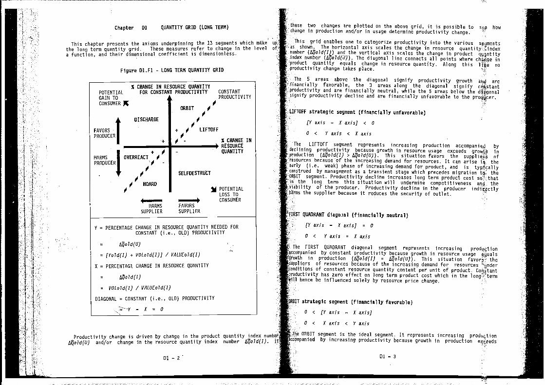
POTENTIALGAIN TOCONSUMER
% CHANGE IN RESOURCE QUANTITYFOR CONSTANT PRODUCTIVITY
DISCHARGE
OVERREACT 0'0 -
0
CONSTANTPRODUCTIVITY
4-
ii
ORBIT 0
FAVORS
PRODUCER
HARMS
PRODUCER
+
these two changes we plotted on the above grid, it is possible to howChapter 01 QUANTITY GRIO (LONG TERN)change in production and/or in usage determine productivity change.
This chapter presents the axioms underpinning the 13 segments which make This grid enables one to categorize productivity into the variousthe long term quantity grid. These measures refer to change in the level of as shown. The horizontal axis scales the change in resource quantity:t'index
number and the vertical axis scales the change in product quantitya function, and their dimensional coefficient is dimensionless.index number The diagonal line connects all points where inproduct quantity equals change in resource quantity. Along this lThe noproductivity change takes place.Figure D1.F1 - LONG TERN QUANTITY GRID
The 5 areas above the diagonal signify productivity growth aS arefinancially favorable, the 3 areas along the diagonal signify coPjstantproductivity and are financially neutral, while the 5 areas below thesignify productivity decline and are financially unfavorable to the
LIFTOFF strategic segment (financially unfavorable)
(Y axis — A' axis) < 0
0 C Y axis < x axis
_________________ __________________
The LIFTOFF segment represents increasing production accompanied bydeclining productivity because growth in resource usage exceeds inproduction > This situation favors the suppliers ofresources because of the increasing demand for resources. It can arise irp theearly (i.e. weak) phase of increasing demand for product, and is typfcally
'Censtrued by management as a transient stage which precedes migration tcu theORBIT segment. Productivity decline increases long term product cost thatin the long term this situation will undermine competitiveness and theviability of the producer. Productivity decline in the producerharms the supplier because it reduces the security of outlet.
FIRST QUADRANT dlagoial (financially neutral)
00
LI FTOFF
0 - % CHANGE INRESOURCEQUANTITY
POTENTIALLOSS TOCONSUMER
0
0
HOARD
HA RN S
SUPPLIER
SELFDESTRLICT
FAVORS
SUPPLIER
Y = PERCENTAGE CHANGE IN RESOURCE QUANTITY NEEDED FORCONSTANT (i.e., OLD) PRODUCTIVITY
=
= [Yold(I) + VOLold(I)) / V/ILUEoId(I)
X = PERCENTAGE CHANGE IN RESOURCE QUANTITY
[Yaxis — Xaxisj = 0
=
0 < Yaxis = Xaxis
= V0Lold(I) / VALUE0Id(I)
DIAGONAL = CONSTANT (i.e., OLD) PRODUCTIVITY
- A' = 0
Productivity change is driven by change in the product quantity index numberand/or change in the resource Quantity index number If,
The FIRST QUADRANT diagonal segment represents increasing prodqctionaccompanied by constant productivity because growth in resource usage ehualsgrowth in production (I4old(I) = This situation favora" thesuppliers of resources because of the increasing demand for resourcesconditions of constant resource quantity content per unit of product.roductivity has zero effect on long term product cost which in the long"term
Will hence be influenced solely by resource price change.
ORBIT strategic segment (financially favorable)
0 < [Y axis — A' axis)
0 < Xaxis C Yaxis
01—2 ' 01—3
irhe ORBIT segment is the ideal segment. It represents increasing produLtionccempanied by increasing productivity because growth in production
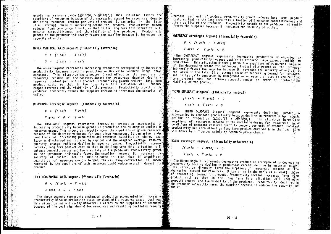
UPPER VERTICAL AXIS segment (financially favorable)
o c (V axis — X axis]
o = Xaxis < Yaxis
The above segment represents increasing production accompanied by increasingproductivity because growth in production occurs while resource usage staysconstant. This situation has a neutral direct effect on the suppliers ofresources because of the constant demand for resources despite decliningresource content per unit of product. Productivity growth reduces long termproduct cost, so that in the long term this situation will enhancecompetitiveness and the viability of the •producer. Productivity growth in theproducer indirectly favors the supplier because it increases the security ofoutlet.
DISCHARGE strategic segment (financially favorable)
o < (Y axis — X axis]
Xaxis < 0 < Yaxis
The DISCHARGE segment represents increasing production accompanied by
increasing productivity because growth in production occurs despite decline irresource usage. This situation directly harms the suppliers of given r::TTTbecause of the decreasing demand for such given resources. It can arise underconditions of increasing production and resource substitution where, say,labor is discharged and replaced by capital and the weighted average resourcequantity change reflects decline in resource usage. Productivityreduces long term product cost so that in the long term this situation willenhance competitiveness and the viability of the producer. Productivity growtFin the producer indirectly favors the supplier because it increases I.security of outlet. Yet it must be borne in mind that ifquantities of resources are discharged, the resulting contraction of inccreceived by the suppliers of such resources could reduce overall demandproduct.
HORIZONTAL AXIS' segment (financially favorable)
0 < (Y axis — X axis]
X axis < 0 = V axis
The above segment represents unchanged production accompanied by increasirproductivity because production stays constant while resource usage declines.This situation has a directly unfavorable effect on the suppliers ofbecause of the declining demand for resources and resulting declining resourcer,
The OVERREACT segment represents decreasing production accompanied byincreasing productivity because decline in resource usage exceeds inproduction. This situation directly harms the suppliers of resourcesef the decreasing for resources. Productivity growth in the prothicerindirectly favors the supplier because it increases the security of Itcan arise in the later (i.e. strong) phase of decreasing demand for product,and is typically construed by management as an essential step to reduce longterm product cost and enhance competitiveness in order to protect theviability of the producer.
THIRD QUADRANT diagonal (financially neutral)
[V axis — Xaxis] = 0
V axis = X axis < o
The THIRD QUADRANT diagonal segment represents decliningmn.nied by constant productivity because decline in resource usage equalsin production = I4old(U)). This situationsuppliers of resources because of the declining demand for resources uqderconditions of constant resource quantity content per unit of product.
r has zero effect on long term product cost which in the longwill hence be influenced solely by resource price change
HOARD strategic segmeit (financially unfavorable)
(V axis — X axis] < 0
V axis < x axis < o
The HOARD segment represents decreasing production accompanied by decreasjngproductivity because decline in production exceeds decline in resourceThis situation directly harms the suppliers of resources because ofecreasing demand for resources. It can arise in the early (i.e. weak) ph4se
F decreasing demand for product. Productivity decline increases longproduct cost so that in the long term this situation willcompetitiveness and the viability of the producer. Productivity decline-inthe producer indirectly harms the supplier because it reduces the security- ofoutlet.
growth in resource usage > This situation favorssuppliers of resources because of the increasing demand for resources despitedeclining resource content per unit of product. It can arise in the later(i.e. strong) phase of increasing demand for product. Productivity growthreduces long term product cost, so that in the long term this situation willenhance competitiveness and the viability of the producer. Productivitygrowth in the producer indirectly favors the supplier because it increases thesecurity of outlet.
content per unit of product. Productivity growth reduces long term productcost, so that in the 1ong term this situation will enhance andthe viability of the producer. Productivity growth in the producerfavors the supplier because it increases the security of outlet. -
OVERREACT 'strategis scgment (financially favorable)
o < (V axis — X axis]
Xaxis < Vaxis < 0
1-
ii.9
Dl—4 DI — 5
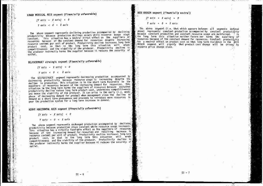
LOWER VERTICAL AXIS segment (financially unfavorable)
(Y axis — X axis] < 0
Y axis C 0 = X axis
The above segment represents declining production accompanied by decliningproductivity because production declines occurs while resource usage stays
constant. This situation has a neutral direct effect on the suppliers of
resources because of the constant demand for resources despite increasingresource content per unit of product. Productivity decline increases long termproduct cost, so that in the long term this situation will erode
competitiveness and the viability of the producer. Productivity decline in
the producer indirectly harms the supplier because it reduces the security of
outlet.
SELFDESTRIJCT strategic segment (financially unfavorable)
(Yaxis — Xaxis] < 0
Yaxis < 0 C laxis
The SELFDESTRLJCT segment represents decreasing production accompanied by
decreasing productivity because resource usage is increasing despite the
decline in production. This situation is in the short term favorable to the
suppliers of resources because of the increasing demand for resources. This
situation in the long term harms the suppliers of resources becauseproductivity decline raises long term product cost, undermines competitivenand hence the viability of the producer. It can arise in the early (i.e. w...,.,phase of decreasing demand for product when management views the decline in
demand as a short term phenomenon and proceeds to introduce more resources to
gear the production system for a long term increase in demand.
RIGHT HORIZONTAL AXIS segment (financially unfavorable)
(Y axis — X axis] < 0
V axis = 0 < X axis
The above segment represents unchanged production accompanied by declininfproductivity because production stays constant while resource usage increases.This situation has a directly favorable effect on the suppliers of resources
because of the increasing demand for resources and resulting increase IT,
resource content per unit of product. Productivity decline increases long ternproduct cost, so that in the long term this situation will erode
competitiveness and the viability of the producer. Productivity decline in
the producer indirectly harms the supplier because it reduces the security or
outlet.
AXIS ORIGIN segment (financially neutral)
[V axis — X axis] = 0
V axis = = X axis
The above segment (i.e. that which appears between all segments definedabove) represents constant production accompanied by constantbecause constant production and constant resource usage are maintained. Inthe long term this situation neither favors nor harms the of
..es because of the constant demand for resources. Constantproduct cost so that long term residence in the AXIS
N segment will signify that product cost change will be drivefl byresource price change alone. I-
— I I
ILLDl — 6
Dl — 7
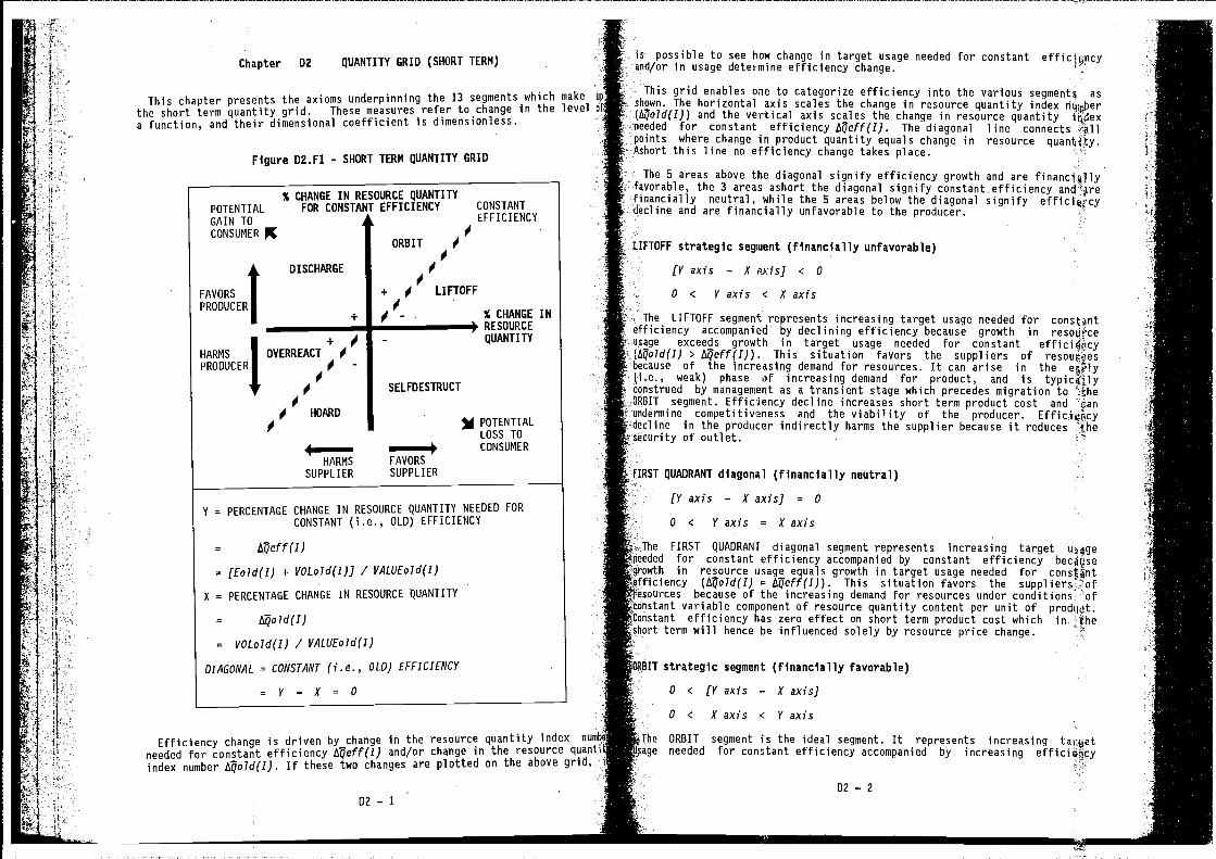
This chapter presents the axioms underpinning the 13 segments which makethe short term quantity grid. These measures refer to change in the levela function, and their dimensional coefficient is dimensionless.
Figure O2.Fl - SHORT TERM QUANTITY GRID
Efficiency change is driven by change in the resource quantity index nun
needed for constant efficiency LØeff(I) and/or change in the resource quantiindex number If these two changes are plotted on the above grid,
I
This grid enables one to categorize efficiency into the various segments asThe horizontal axis scales the change in resource quantity index
(/4old(I)) and the vertical axis scales the change in resource quantityneeded for constant efficiency The diagonal line connects 'Callpeints where change in product quantity equals change in resource quantity.Ashort this line no efficiency change takes place.
The 5 areas above the diagonal signify efficiency growth and arefavorable, the 3 areas ashort the diagonal signify constant efficiencyfinancially neutral, while the 5 areas below the diagonal signify efficlqncydecline and are financially unfavorable to the producer.
The LIFTOFF segment represents increasing target usage needed for constantefficiency accompanied by declining efficiency because growth in resource
exceeds growth in target usage needed for constant((I) > This situation favors the suppliers of
because of the increasing demand for resources. It can arise in the eflly(i.e., weak) phase of increasing demand for product, and is
by management as a transient stage which precedes migration toIT segment. Efficiency decline increases short term product cost and dan
'mine competitivaness and the viability of the producer..d in the producer indirectly harms the supplier because it reduces :the
(rity of outlet.
:::T QUADRANT diagonal (financially neutral)
(V axis — X axis] = 0
0 < V axis = axis
The FIRST QUADRANT diagonal segment represents increasing target usAgeeded for constant efficiency accompanied by constant efficiency becAuse
h in resource usage equals growth in target usage needed foriciency = This situation favors the
sources because of the increasing demand for resources under conditions ofvariable component of resource quantity content per unit of
,ftonstant efficiency has zero effect on short term product cost which in jheiert term will hence be influenced solely by resource price change.
T strategic segment (financially favorable)
0 < [V axis — K axis]
0 < Xaxis < Vaxis
he ORBIT segment is the ideal segment. It represents increasing targetneeded for constant efficiency accompanied by increasing
D2 — 2
Chapter 02 QUANTITY GRID (SHORT TERN)possible to see how change in target usage needed for constant effickpcy
and/or in usage determine efficiency change.
CONSTANTEFFICIENCY
% CHANGE IN+ RESOURCE
QUANTITY
LIFTOFF strategic segment (financially unfavorable)
1.
if
t
(V axis — K axis] < 0
0 < Yaxis < Xaxis
% CHANGE IN RESOURCE QUANTITYPOTENTIAL FOR CONSTANT EFFICIENCYGAIN TOCONSUMER % I
ORBIT #
DISCHARGE IFAVORS + p4 LIFTOFF
PRODUCER I+ 0-•
+1HARMS OVERREACT #PRODUCER p4 -
SELFOESTRUCT
HOARDPOTENTIALLOSS TOCONSUMER
HARMS FAVORS
SUPPLIER SUPPLIER
Y = PERCENTAGE CHANGE IN RESOURCE QUANTITY NEEDED FOR
CONSTANT (i.e., OLD) EFFICIENCY
=
= (Eold(I) + VOLold(I)] / VALUE01d(I)
X = PERCENTAGE CHANGE IN RESOURCE QUANTITY
=
= VOLo1d(I) / VALUEoIO(I)
DIAGONAL = CONSTANT (i.e., OLO) EFFICIENCY
=y—x=0
D2 — 1

because growth in target usage needed for constant efficiency exceeds gro"in resource usage > This situation favors the suppliof resources because of the increasing demand for resources despite declini.variable component of resource content per unit of product. It can arisethe later (i.e. strong) phase of increasing demand for product.growth reduces short term product cost, so that in the short term this -
situation will enhance competitiveness and the viability of the producer.
Efficiency growth in the producer indirectly favors the supplier because itincreases the security of outlet.
UPPER VERTICAL AXIS segment (financially favorable)
o < fY axis — K axis]
0 = K axis C Y axis
The above segment represents increasing target usage needed for constant
efficiency accompanied by increasing efficiency because growth in target usageneeded for constant efficiency occurs while resource usage stays constant.
This situation has a neutral direct effect on the suppliers of resources
because of the constant demand for resources despite declining resource
content per unit of product. Efficiency growth reduces short term product
cost, so that in the short term this situation will enhance competitiveness
and the viability of the producer. Efficiency growth in theindirectly favors the supplier because it increases the security of outlet.
DISCHARGE strategic segment (financially favorable)
o c fYaxis — Xaxis]
K axis c 0 < Y axis
The DISCHARGE segment represents increasing target usage needed for constaiefficiency accompanied by increasing efficiency because growth in targetneeded for constant efficiency occurs despite decline in resource usage.situation directly harms the suppliers of given resources because of Udecreasing demand for such given resources. It can arise under conditions' ci
increasing target usage needed for constant efficiency and resourci
substitution where, say, labor is discharged and replaced by capital and thi
weighted average resource quantity change reflects decline in resourceEfficiency increase reduces short term product cost so that in the short tthis situation will enhance competitiveness and the viability of the producerEfficiency growth in the producer indirectly favors the supplier because I,
increases the security of outlet. Yet it must be borne in mind that i
significant quantities of resources are discharged, the resulting contractiof income received by the suppliers of such resources could reduce overeli.
demand for product.
LEFT HORIZONTAL AXIS segment (financially favorable)
o < fY axis — K axis]
K axis < 0 = Y axis
The above segment represents unchanged target usage needed forefficiency accompanied by increasing efficiency because target usage neec
02 — 3
for constant efficiency stays constant while resource usage declines. Thissituation has a directly unfavorable effect on the suppliers ofbecause of the decUning demand for resources and resulting declining ra4ourcecontent per unit of product. Efficiency growth reduces short termcost, so that in the short term this situation will enhanceend the viability of the producer. Efficiency growth in the prAducerindirectly favors the supplier because it increases the security of outflt.
OVERREACT strategis segment (financially favorable)
0 c (V axis — K axis]
Kaxis C Yaxis < 0
The OVERREACT segment represents decreasing target usage needed forefficiency accompanied by increasing efficiency because decline in rOourceusage exceeds decline in target usage needed for constant efficiency,? Thissituation directly harms the suppliers of resources because of the decreasingdemand for resources. Efficiency growth in the producer indirectly favori thesupplier because it increases the security of outlet. It can arise thelater (i.e. strong) phase of decreasing demand for product, and is typicallyconstrued by management as an essential step to reduce short term costand enhance competitiveness in order to protect the viability of the prQAucer.
THIRD QUADRANT diagunal (financially neutral)
[Y axis — K axis] = 0
The THIRD QUADRANT diagonal segment represents declining target usage k5peded'ir constant efficiency accompanied by constant efficiency because decljeje inresource equals decline in target usage needed for constant
= LtQeff(J)). This situation harms the suppliers of resourcesthe declining demand for resources under conditions of constant variable...,..,it of resource quantity content per unit of product. Cogstantciency has zero effect on short term product cost which in the short? term
11 hence be influenced solely by resource price change.
WARD strategic segment (financially unfavorable)
(Y axis — K axis] < 0
HOARD segment represents decreasing target usage needed foraccompanied by decreasing efficiency because decline in target
e needed for constant efficiency exceeds decline in resource usage.[This,uation directly harms the suppliers of resources because of the
lenand for resources. It can arise in the early (i.e. weak) pha,4 ofJecreasing demand for product. Efficiency decline increases short term pSduct
so that in the short term this situation will undermineI the viability of the producer. Efficiency decline in therectly harms the supplier because it reduces the security of outlet.;
V axis < K axis < 0
V axis = K axis C 0
D2 — 4
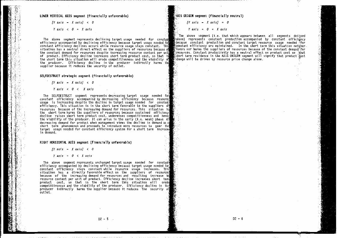
The above segment represents declining target usage needed for constao.efficiency accompanied by declining efficiency because target usage needed forconstant efficiency declines occurs while resource usage stays constant. Thisituation has a neutral direct effect on the suppliers of resources becausethe constant demand for resources despite increasing resource content per oniof product. Efficiency decline increases short term product cost, so that i
the short term this situation will erode competitiveness and the viabilitythe producer. Efficiency decline in the producer indirectly harms thosupplier because it reduces the security of outlet.
SELFOESTRUCT strategic segment (financially unfavorable)
(Y axis — X axis] < 0
Y axis < 0 c X axis
The SELFDESTRUCT segment represents decreasing target usage needed forconstant efficiency accompanied by decreasing efficiency because resource.usage is increasing despite the decline in target usage needed forefficiency. This situation is in the short term favorable to the suppliers
of the increasing demand for resources. This situation in?
the short term harms the suppliers of resources because sustained efficiencydecline raises short term product cost, undermines competitiveness and hencrthe viability of the producer. It can arise in the early (i.e. weak) phase of
decreasing demand for product when management views the decline in demand asshort term phenomenon and proceeds to introduce more resources to gear thetarget usage needed for constant efficiency system for a short term increasein demand.
RIGHT HORIZONTAL AXIS segment (financially unfavorable)
[V axis — X axis] C 0
The above segment represents unchanged target usage needed forefficiency accompanied by declining efficiency because target usage needed farconstant efficiency stays constant while resource usage increases. Thin;situation has a directly favorable effect on the suppliers of resourceo,because of the increasing demand for resources and resulting increase io,resource content per unit of product. Efficiency decline increases shortproduct cost, so that in the short term this situation will erodecompetitiveness and the viability of the producer. Efficiency decline in theproducer indirectly harms the supplier because it reduces the security ofoutlet.
Y axis = 0 c X axis
AXIS ORIGIN segment (financially neutral)
[V axis — XaxisJ = 0
Yaxis = 0 = Xaxis
The above segment (i.e. that which appears between all segments deflnedabove) represents constant production accompanied by constantbecause constant production and constant target resource usage neededconstant efficiency are maintained. In the short term this situation nelkher.favors nor harms the soppl i ers of resources because of the constantresources. Constant productivity has a neutral effect on product cost soshort term residence in the AXIS ORIGIN segment will signify that productchange will be driven by resource price change alone.
LOWER VERTICAL AXIS segment (financially unfavorable)
[V axis — X axis] < 0
V axis c 0 = X axis
ftii
ft
D2—5 D2 — 6
a
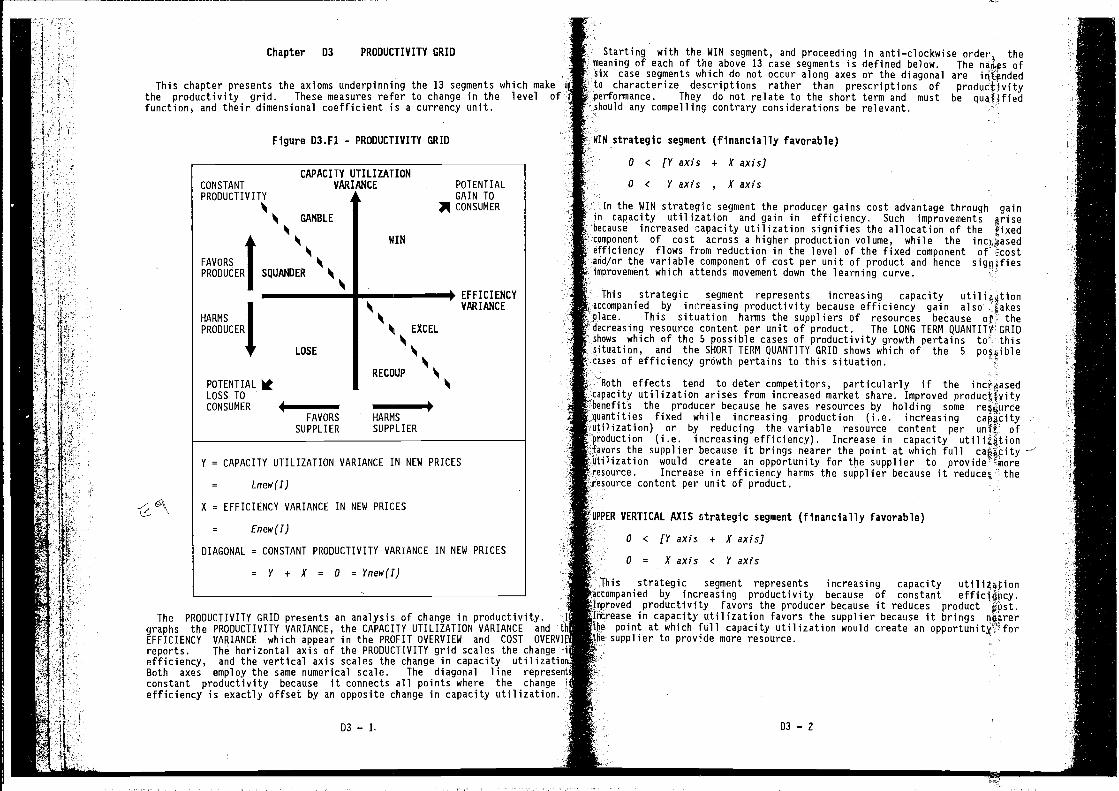
Chapter D3 PRODUCTIVITY GRID
This chapter presents the axioms underpinning the 13 segments which make up
the productivity grid. These measures refer to change in the level offunction, and their dimensional coefficient is a currency unit.
Figure D3.Fl - PRODUCTIVITY GRID
= Enew(I)
DIAGONAL = CONSTANT PRODUCTIVITY VARIANCE IN NEW PRICES
= Y + X = 0 = Ynew(I)
The PRODUCTIVITY GRID presents an analysis of change in productivity. I
graphs the PRODUCTIVITY VARIANCE, the CAPACITY UTILIZATION VARIANCE and th
EFFICIENCY VARIANCE which appear in the PROFIT OVERVIEW and COST OVERVIE
reports. The horizontal axis of the PRODUCTIVITY grid scales the change i
efficiency, and the vertical axis scales the change in capacity utilizationBoth axes employ the same numerical scale. The diagonal line representconstant productivity because it connects all points where the change i
efficiency is exactly offset by an opposite change in capacity utilization.
D3 — 1.
Starting with the WIN segment, and proceeding in anti—clockwise order, themeaning of each of the above 13 case segments is defined below. The ofsix case segments which do not occur along axes or the diagonal are intendedte characterize descriptions rather than prescriptions ofperformance. They do not relate to the short term and must be quaiifiedshould any compelling contrary considerations be relevant.
WIN strategic segment (financially favorable)
0 c [V axis + Xaxis]
0 c Vaxis , Xaxis
In the WIN strategic segment the producer gains cost advantage through gainin capacity utilization and gain in efficiency. Such improvements prisebecause increased capacity utilization signifies the allocation of the fixedcomponent of cost across a higher production volume, while the incr4asedefficiency flows from reduction in the level of the fixed component of
cost and hence signifiesImprovement which attends movement down the learning curve. -
This strategic segment represents increasing capacityaccompanied by increasing productivity because efficiency gain also fakesplace. This situation harms the suppliers of resources because of' thedecreasing resource content per unit of product. The LONG TERM QUANTITY GRIDshows which of the 5 possible cases of productivity growth pertains to' thissituation, and the SHORT TERN QUANTITY GRID shows which of the 5
eases of efficiency grOwth pertains to this situation.
Both effects tend to deter competitors, particularly if thecapacity utilization arises from increased market share. Improved productivity
Thenefits the producer because he saves resources by holding some re$urcefixed while increasing production (i.e. increasing caflcity
utilization) or by reducing the variable resource content per unit of-production (i.e. increasing efficiency). Increase in capacity utili2ftion-'favors the supplier because it brings nearer the point at which full —
would create an opportunity for the supplier toIncrease in efficiency harms the supplier because it the
'resource content per unit of product.
UPPER VERTICAL AXIS Ltrategic segment (financially favorable)
0 < [V axis + X axis]
0 = X axis c V axis
This strategic segment represents increasing capacityaccompanied by increasing productivity because of constant efficj4pcy.Improved productivity favors the producer because it reduces productIncrease in capacity utilization favors the supplier because it bringsthe point at which full capacity utilization would create an opportunity' forthe supplier to more resource.
CAPACITY UTILIZATIONVARIANCE
WIN
POTENTIALGAIN TOCONSUMER
+ EFFICIENCYVARIANCE
CONSTANTPRODUCTIVITY
b4 GANBLE
tFAVORSPRODUCER SQUANDER
I,
HA RN S
PRODUCER
POTENTIALLOSS TOCONSUMER
I''I EXCEL
LOSE
FAVORS
SUPPLIER
RECOUP
HA RN S
SUPPLIER
Y = CAPACITY UTILIZATION VARIANCE IN NEW PRICES
= Lnew(I)
X = EFFICIENCY VARIANCE IN NEW PRICES
03 — 2
S
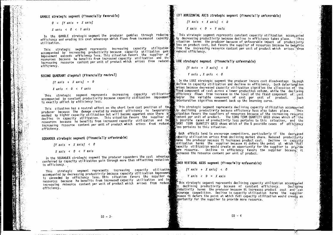
GAMBLE strategic segment (financially favorable)
o < (Y axis + X axis]
X axis < 0 < Y axis
In the GAMBLE strategic segment the producer gambles through reducirefficiency and eroding his cost advantage which flows from increased capacilutilization.
This strategic segment represents increasing capacity utilizaticaccompanied by increasing productivity because capacity utilization gaff
impovement exceeds efficiency loss. This situation favors the supplier ci
resources because he benefits from increased capacity utilization and tffincreasing resource content per unit of product which arises from reduced.
efficiency.
SECOND QUADRANT diagonal (financially neutral)
(V axis + X axis] = 0
X axis < 0 C Y axis
This strategic segment represents increasing capacity utilizataccompanied by constant productivity because capacity utilization impovemen
is exactly offset by efficiency loss.
This situation has a neutral effect on the short term cost position of t,
producer because the damage created by reduced efficiency is temporai'i.
masked by higher capacity utilization but will become apparent once there i
decline in capacity utilization. This situation favors the supplierresources because he benefits from increased capacity utilization and tL
increasing resource content per unit of product which arises froni reduce
efficiency.
SQUANDER strategic segment (financially unfavorable)
(Y axis + K axis] C 0
Kaxis C 0 < Y axis
In the SQUANDER strategic segment the producer squanders the cost advantag
conferred by capacity utilization gain through more than offsetting reductirin efficiency.
This strategic segment represents increasing capacity utilizattcaccompanied by decreasing productivity because capacity utilization impovemer
is exceeded by efficiency loss. This situation favors the supplier c
resources because he benefits from increased capacity utilization and rincreasing resource content per unit of product which arises from reduu
efficiency.
This strategic segment represents constant capacity utilizationdecreasing productivity because decline in efficiency takes place. This
tuation harms the producer because of unfavorable impact of productjvityis on product cost, but favors the supplier of resources because he
the increasing resource content per unit of product which arises ,cfromefficiency.
In the LOSE strategic segment the producer incurs cost disadvantage'dine in capacity utilization and decline in efficiency. •Suchises because decreased capacity utilization signifies the allocation of the
rnmnnn 'cnt of cost across a lower production volume, while the decflpingncy i from increase in the level of the fixed component of: cost
id/or the variable component of cost per unit of product. Suchsignifies movement back up the learning curve.
This strategic segment represents declining capacity utilizationry declining productivity because efficiency loss also takes place.
uation favors the suppliers of resources because of the increasing resQurceintent per unit of product. The LONG TERM QUANTITY GRID shows which thepossible cases of productivity loss pertains to this situation, and the
ORT TERM QUANTITY GRID shows which of the 5 possible cases of efficilcncypertains to this situation.
Both effects tend to encourage competitors, particularly if theapacity utilization arises from declining market share. Reduced productivity
...s the producer because it increases product cost. Decline inlization harms the supplier because it defers the point at which ]'ullacity utilization would create an opportunity for the supplier to prawidee resource. Decline in efficiency favors the supplier it
the resource content per unit of product.
VERTICAL AXIS segment (financially unfavorable)
Vaxis C 0 = Kaxis
This strategic segment represents declining capacity utilization accomp4flieddeclining productivity because of constant efficiency. Decltgiing
:cductivity harms the producer because it increases product cost andcompetition. Decline in capacity utilization harms the supplier
ause it defers the point at which full capacity utilization would anportunity for the supplier to provide more resource.
LEFT HORIZONTAL AXIS strategic segment (financially unfavorable)
(V axis + K axis] < 0
K axis < 0 = V axis
LOSE strategic segmeut (financially unfavorable)
(V axis + K axis] C 0
V axis , K acis C 0
:1
.4
I.
(V axis + Kaxis] C 0
I
03 — 3 03 — 4
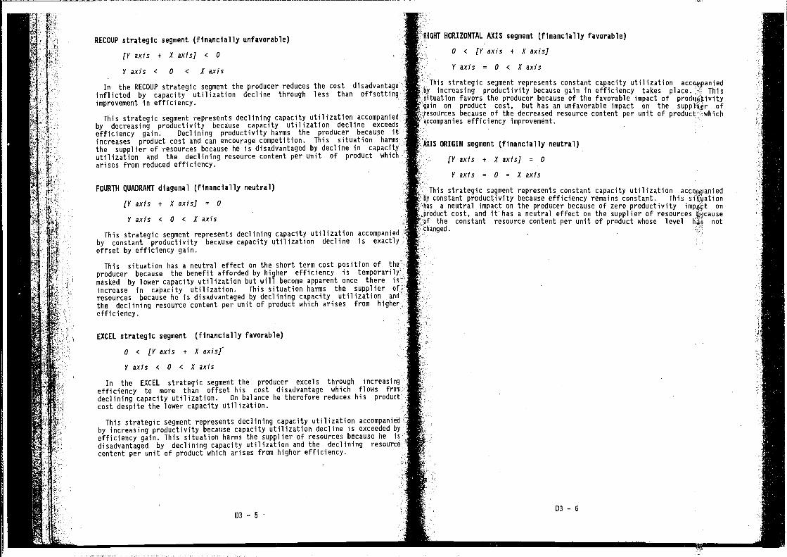
RECOUP strategic segment (financially unfavorable)
(Y axis + X axis] < 0
Y axis ( 0 < X axis
In the RECOUP strategic segment the producer reduces the cost disadvantageinflicted by capacity utilization decline through less than offsettingimprovement In efficiency.
This strategic segment represents declining capacity utilization accompaniedby decreasing productivity because capacity utilization decline exceedsefficiency gain. Declining productivity harms the producer because itincreases product cost and can encourage competition. This situation harms
the supplier of resources because he is disadvantaged by decline in capacityutilization and the declining resource content per unit of product whicharises from reduced efficiency.
FOURTH QUADRANT diagonal (financially neutral)
EY axis + X axis] = 0
Y axis < 0 < X axis
This strategic segment represents declining capacity utilization accompaniedby constant productivity because capacity utilization decline is exactlyoffset by efficiency gain.
This situation has a neutral effect on the short term cost position of theproducer because the benefit afforded by higher efficiency is temporarilymasked by lower capacity utilization but will become apparent once there isincrease in capacity utilization. This situation harms the supplier ofresources because he is disadvantaged by declining capacity utilization and
the declining resource content per unit of product which arises from higherefficiency.
EXCEL strategic segment (financially favorable)
0 < [Y axis + X axis]
Y axis < 0 < X axis
In the EXCEL strategic segment the producer excels through increasingefficiency to more than offset his cost disadvantage which flows fromdeclining capacity utilization. On balance he therefore reduces his productcost despite the lower capacity utilization.
This strategic segment represents declining capacity utilization accompaniedby increasing productivity because capacity utilization decline is exceeded byefficiency gain. This situation harms the supplier of resources because he isdisadvantaged by declining capacity utilization and the decliningcontent per unit of product which arises from higher efficiency.
This strategic segment represents constant capacity utilizationincreasing productivity because gain in efficiency takes place. This
::tion favors the producer because of the favorable impact of.n on product cost, but has an unfavorable impact on the suppler ofsources because of the decreased resource content per unit ofcompanies efficiency improvement.
This strategic segment represents constant capacity utilizationby constant productivity because efficiency remains constant. Thishas a neutral impact on the producer because of zero productivity onproduct cost, and it has a neutral effect on the supplier of resourcesof the constant resource content per unit of product whose level notchanged.
RIGHT HORIZONTAL AXIS segment (financially favorable)
o < (V axis + X axis]
V axis 0 < X axis
S ORIGIN segment (financially neutral)
(Y axis + K axis] = 0
Y axis = 0 = K axis
D3 — 5D3 — 6
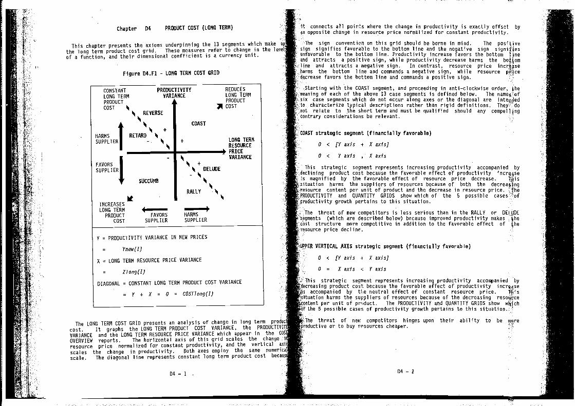
Chapter 04 PRODUCT COST (LONG TERM)
This chapter presents the axioms underpinning the 13 segments which makethe long term product cost grid. These measures refer to change in the levelof a function, and their dimensional coefficient is a currency unit.
V = PRODUCTIVITV VARIANCE IN NEW PRICES
= Ynew(I)
X = LONG TERM RESOURCE PRICE VARIANCE
= Zlong(I)
DIAGONAL = CONSTANT LONG TERM PRODUCT COST VARIANCE
= Y + X = 0 = COSTlong(I)
The LONG TERM COST GRIO presents an analysis of change in long term prodaj
cost. It graphs the LONG TERM PROOUCT COST VARIANCE, the PRODUCTIVI1
VARIANCE and the LONG TERM RESOURCE PRICE VARIANCE which appear in the 0
OVERVIEW reports. The horizontal axis of this grid scales the change
resource price normalized for constant productivity, and the vertical a:
scales the change in productivity. Both axes employ the same numerici
scale. The diagonal line represents constant long term product cost
04—1
It connects all points where the change in productivity is exactly offset byan opposite change in resource price normalized for constant productivity.
The sign convention on this grid should be borne in mind. The positivesign signifies favorable to the bottom line and the negative sign signiFIesanfavorable to the bottom line. Productivity increase favors the bottom flneand attracts a positive sign, while productivity decrease harms theline and attracts a negative sign. In contrast, resource price increjseharms the bottom line and commands a negative sign, while resourcedecrease favors the bottom line and commands a positive sign.
Starting with the COAST segment, and proceeding in anti—clockwise order, themeaning of each of the above 13 case segments is defined below. The nameçofSix case segments which do not occur along axes or the diagonal are inteuded4a characterize typical descriptions rather than rigid definitions. They
relate to the short term and must be qualified should any compellingcontrary considerations be relevant.
strategic segment (financially favorable)
o < [V axis + X axis]
o < Yaxis , Xaxis
This strategic segment represents increasing productivity accompanied byproduct cost because the favorable effect ol productivity incre3se
magnified by the favorable effect of resource price decrease. Thisharms the suppliers of resources because of both the
source content per unit of product and the decrease in resource price. - theIDUCTIVITY and QUANTITY GRIDS show which of the 5 possible cases of
growth pertains to this situation.
The threat of new competitors is less serious than in the RALLY or DELUDEsegments (which are described below) because improved productivity makes
structure more competitive in addition to the favorable effect of:-resource price decline.
VERTICAL AXIS strategic segment (financially favorable)
o < [V axis 4 X axis]
0 = Xaxis < Yaxis
is strategic segment represents increasing productivity accompanied bycreasing product cost because the favorable effect of productivity
accompanied by the neutral effect of constant resource price, istuation harms the suppliers of resources because of the decreasing resoàtcefltent per unit of prriduct. The PRODUCTIVITY and QUANTITY GRIDS showthe S possible cases of productivity growth pertains to this situation.
he threat of new competitors hinges upon their ability to beor to buy rosources cheaper.
Figure D4.F1 - LONG TERM COST GRID
PRODUCTIVITYVARIAMCE
ERSE
+RETARD
+
COAST
REDUCES
LONG TERMPRODUCT
$ COST
LOMG TERMRESOURCE
—0 PRICEVARIANCE
CONSTANTLONG TERMPRODUCT
COST
HARMS
SUPPLIER
FAVORS
SUPPLIER
INCREASESLONG TERM
PRODUCTCOST
+DELUDE
SUCCUMB
RALLY
4 p
FAVORS HARMS
SUPPLIER SUPPLIER
I04 — 2
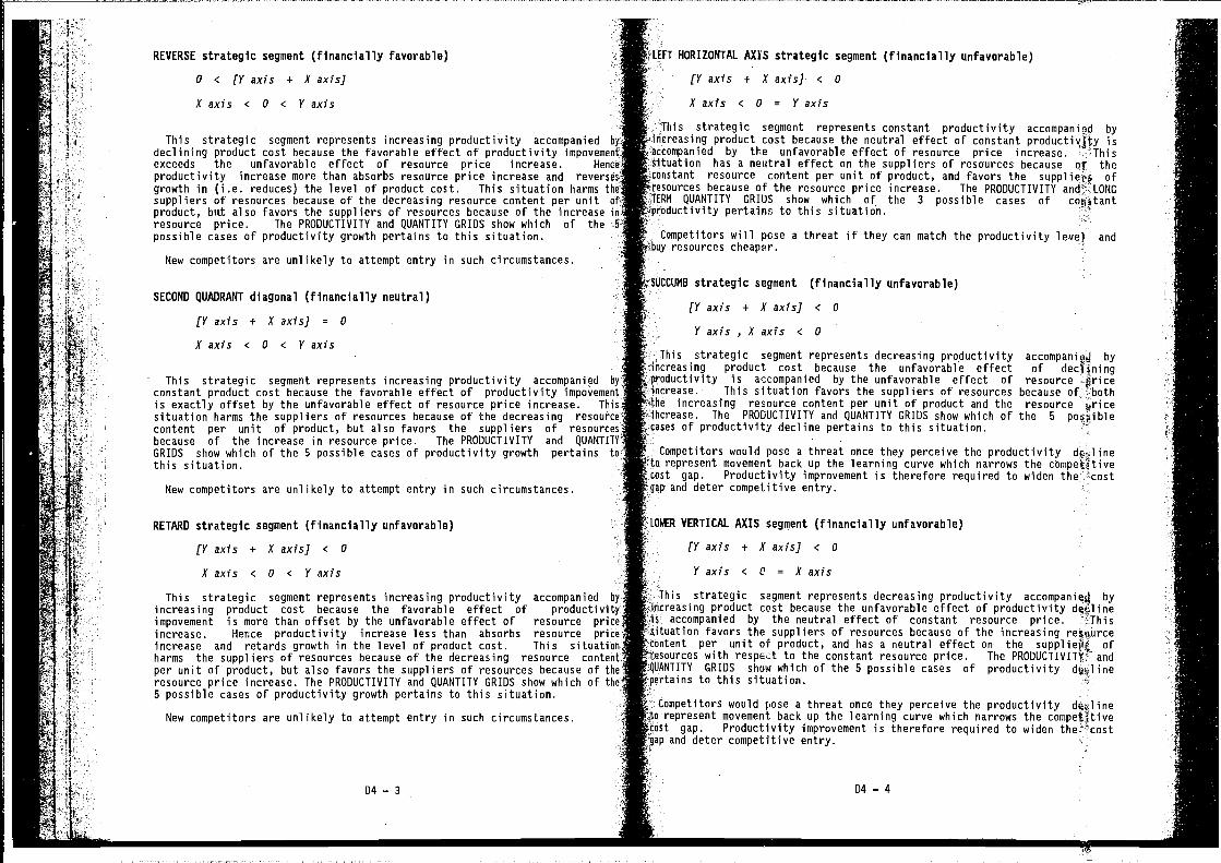
This strategic segment represents increasing productivity accompanied by.declining product cost because the favorable effect of productivity impovementexceeds the unfavorable effect of resource price increase.productivity increase more than absorbs resource price increase and reversesgrowth in (i.e. reduces) the level of product cost. This situation harms thesuppliers of resources because of the decreasing resource content per unit ofproduct, bu.t also favors the suppliers of resources because of the increase inresource price. The PRODUCTIVITY and QUANTITY GRIDS show which of the 5
possible cases of productivity growth pertains to this situation.
New competitors are unlikely to attempt entry in such circumstances.
SECOND QUADRANT diagonal (financially neutral)
(Yaxis + Kaxis] = 0
Xaxis < 0 < Yaxis
This strategic segment represents increasing productivity accompanied by
constant product cost because the favorable effect of productivity impovementis exactly offset by the unfavorable effect of resource price increase. Thissituation harms the suppliers of resources because of the decreasing resourcecontent per unit of product, but also favors the suppliers of resourcesbecause of the increase in resource price. The PRODUCTIVITY and QUANTITY
GRIDS show which of the 5 possible cases of productivity growth pertains tothis situation.
New competitors are unlikely to attempt entry in such circumstances.
RETARD strategic segment (financially unfavorable)
(Yaxis + Xaxis] c 0
X axis < 0 < Y axis
This strategic segment represents increasing productivity accompanied by
increasing product cost because the favorable effect of productivityimpovement is more than offset by the unfavorable effect of resource priceincrease. Hence productivity increase less than absorbs resource priceincrease and retards growth in the level of product cost. This situation,harms the suppliers of resources because of the decreasing resource contenUper unit of product, but also favors the suppliers of resources because of theresource price increase. The PRODUCTIVITY and QUANTITY GRIDS show which of thel5 possible cases of productivity growth pertains to this situation.
New competitors are unlikely to attempt entry in such circumstances.
HORIZONTAL AXiS strategic segment (financially unfavorable)
(Y axis + X axis] < 0
Xaxis < o = Yaxis
This strategic segment represents constant productivity accompanied byproduct cost because the neutral effect of constant productivity is
accompanied by the unfavorable effect of resource price increase. Thishas a neutral effect on the suppliers of resources because of the
constant resource content per unit of product, and favors the ofPesources because of the resource price increase. The PRODUCTIVITY and'. LONG
:TERM QUANTITY GRIDS show which of the 3 possible cases ofvproductivity pertains to this situation.
Competitors will pose a threat if they can match the productivity levei and-buy resources cheaper.
strategic segment (financially unfavorable)
(Y axis + X axis] c 0
V axis , X axis < 0
• This strategic segment represents decreasing productivity byproduct cost because the unfavorable effect of
productivity is accompanied by the unfavorable effect of resourceIncrease This situation favors the suppliers of resources because of
increasing resource content per unit of product and the resource ericeThe PRODUCTIVITY and QUANTITY GRIDS show which of the 5
cases of productivity decline pertains to this situation.
Competitors would pose a threat once they perceive the productivity dç;linerepresent movement back up the learning curve which narrows the
cost gap. Productivity improvement is therefore required to widen the•gap and deter competitive entry.
VERTICAL AXIS segment (financially unfavorable)
(Y axis + X axis] c 0
Yaxis c 0 = Xaxis
This strategic segment represents decreasing productivity accompanied byIncreasing product cost because the unfavorable effect of productivity dflline
:is accompanied by the neutral effect of constant resource price. TThisfavors the suppliers of resources because of the increasing
per unit of product, and has a neutral effect on the ofresources with respect to the constant resource price. The PRODUCTIVITy- andQUANTITY GRIDS show which of the 5 possible cases of productivitypertains to this situation.
Competitors would pose a threat once they perceive the productivity declineto represent movement back up the learning curve which narrows the competitivetest gap. Productivity improvement is therefore required to widengop and deter competitive entry.
REVERSE strategic segment (financially favorable)
o < (V axis + X axis]
X axis c 0 < Y axis
D4 — 3 D4—4
11
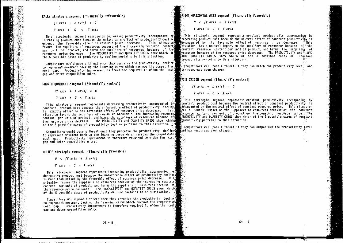
RALLY strategic segment (financially unfavorable)
(Y axis + X axis] c U
Yaxis < 0 C Xaxis
This strategic segment represents decreasing productivity accompaniedincreasing product cost because the unfavorable effect of productivity declineexceeds the favorable effect of resource price decrease. This situationfavors the suppliers of resources because of the increasing resource contentper unit of product, and harms the suppliers of resources because of the
resource price decrease. The PRODUCTIVITY and QUANTITY GRIDS show which of
the 5 possible cases of productivity decline pertains to this situation.
Competitors would pose a threat once they perceive the productivity declirto represent movement back up the learning curve which narrows the -
cost gap. Productivity improvement is therefore required to widen the cost
gap and deter competitive entry.
FOURTH QUADRANT diagonal (financially neutral)
(V axis + XaxisJ = 0
Y axis < 0 < X axis
This strategic segment represents decreasing productivity accompanied bj
constant product cost because the unfavorable effect of productivity declinis exactly offset be the favorable effect of resource price decrease. TT
situation favors the suppliers of resources because of the increasingcontent per unit of product, and harms the suppliers of resources because i
the resource price decrease. The PRODUCTIVITY and QUANTITY GRIDS show whiiof the 5 possible cases of productivity decline pertains to this situation.
Competitors would pose a threat once they perceive the productivity declineto represent movement back up the learning curve which narrows the competitivecost gap. Productivity improvement is therefore required to widen thegap and deter competitive entry.
DELUDE strategic segment (financially favorable)
0 < (V axis + X axis]
V axis < 0 < X axis
This strategic segment represents decreasing productivity accompanied frdecreasing product cost because the unfavorable effect of productivity decliois more than offset by the favorable effect of resource price decrease. T:.
situation favors the suppliers of resources because of the increasing resourcontent per unit of product, and harms the suppliers of resources becausethe resource price decrease. The PRODUCTIVITY and QUANTITY GRIDS show wh
of the 5 possible cases of productivity decline pertains to this situation.
Competitors would pose a threat once they perceive the productivity dec11
to represent movement back up the learning curve which narrows the competiticost gap. Productivity improvement is therefore required to widen the cgap and deter competitive entry.
IT HORIZONTAL AXIS segment (financially favorable)
0 < (V axis + X axis]
Y axis = 0 < X axis
This strategic segment represents constant productivity accompanicif byiecreasing product cost because the neutral effect of constant isaccompanied by the favorable effect of resource price decrease.;ituation has a neutral impact on the suppi iers of resources because of the:onstant resource content per unit of product, and harms the ofresources because of the resource price decrease. The PRODUCTIVITY and -IONG
QUANTITY GRIDS show which of the 3 possible cases ofroductivity pertains to this situation.
Competitors will pose a threat if they can match the productivity level andy resources even cheaper.
ORIGIN segment (financially neutral)
(V axis + Xaxis] = 0
V axis = U = X axis
This strategic segment represents constant productivity accompanieq bytonstant product cost because the neutral effett of constant productivity isaccompanied by the neutral effect of constant resource price. This
a neutral impact on the suppliers of resources because of the conttanturce content per unit of product and the constant resource price.7 The
.,.JUCTIVITY mnd QUANTITY GRIDS show which of the 3 possible cases of conflant'oductivity pertains to this situation.
will pose a threat if they can outperform the productivityend buy resources even cheaper.
U
04 — 5 04 — 6
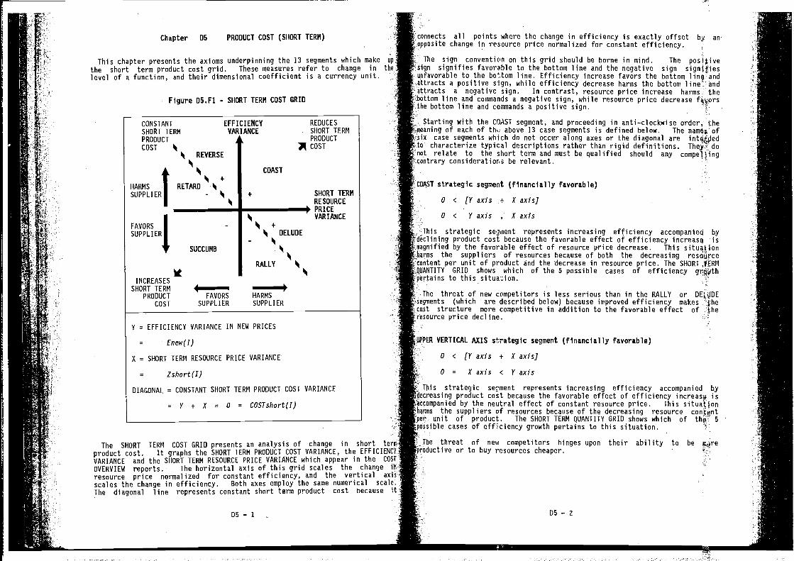
L
Chapter D5 PRODUCT COST (SHORT TERM)
This chapter presents the axioms underpinning the 13 segments which makethe short term product cost grid. These measures refer to change inlevel of a function, and their dimensional coefficient is a currency unit.
Figure D5.F1 - SHORT TERM COST GRID
all points where the change in efficiency is exactly offset anepposite change in resource price normalized for constant efficiency.
The sign conventipn on this grid should be borne in mind. The positivesign signifies favorable to the bottom line and the negative sign signjties
to the bottom line. Efficiency increase favors the bottom;ts a positive sign, while efficiency decrease harms the bottom line and'i a negative sign. In contrast, resource price increase harms the
tom line and commands a negative sign, while resource price decreasebottom line and commands a positive sign.
Starting with the COAST segment, and proceeding in anti—clockwise theof each of thti above 13 case segments is defined below. The namea of
a case segments which do not occur along axes or the diagonal arecharacterize typical descriptions rather than rigid definitions. do
it relate to the short term and must be qualified should anycontrary considerations be relevant. -
I strategic segment (financially favorable)
0 c [Y axis X axis]
CONSTANT EFFICIENCY REDUCES
SHORT TERM VARIANCE SHORT TERM
PRODUCT PRODUCT
COST COST
REVERSE
Ii
ICOAST
HARMS RETARD
SUPPLIER - + SHORT TERMRESOURCE
•j PRICE
VARIANCE
FAVORS +SUPPLIER b4 DELUDE
-SUCCUMB
RALLY
INCREASESSHORT TERN
PRODUCT FAVORS HARMS
COST SUPPLIER SUPPLIER
V = EFFICIENCY VARIANCE IN NEW PRICES
= Enew(I)
x = SHORT TERM RESOURCE PRICE VARIANCE
= Zshort(I)
DIAGONAL = CONSTANT SHORT TERM PRODUCT COST VARIANCE
= Y + X = 0 = CoSTshort(I)
The SHORT TERM COST GRID presents an analysis of change in short tproduct cost. It graphs the SHORT TERM PRODUCT COST VARIANCE, theVARIANCE and the SHORT TERM RESOURCE PRICE VARIANCE which appear in the COS
OVERVIEW reports. The horizontal axis of this grid scales the changeresource price normalized for constant efficiency, and the vertical a'"scales the change in efficiency. Both axes employ the same numerical scale.The diagonal line represents constant short term product cost because
05 — 1
o < Y axis , X axis
nis strategic segnent represents increasing efficiency accompanied bylining product cost because the favorable effect of efficiency increase isnified by the favorable effect of resource price decrease. This situationins the suppliers of resources because of both the decreasing resdurce
t per unit of product and the decrease in resource price. The SHORTV GRID shows which of the 5 possible cases of efficiency
ains to this situation.
The threat of new competitors is less serious than in the RALLY or OEIVOEegments (which are described below) because improved efficiency makes 4he
structure more competitive in addition to the favorable effect ofresource price decline, -
ER VERTICAL AXIS strategic segment (financially favorable)
0 < (Y axis + X axis]
0 = Kaxis < Yaxis
"s strategic segment represents increasing efficiency accompanied bylecreasing product cost because the favorable effect of efficiency increasv isccompanied by the neutral effect of constant resource price. This situatfonarms the suppliers of resources because of the decreasing resourcer unit of product. The SHORT TERM QUANTITY GRID shows which of thp 5
ssible cases of efflciency growth pertains to this situation. •
¶ke threat of new competitors hinges upon their ability to bemductive or to buy resources cheaper.
05 — 2
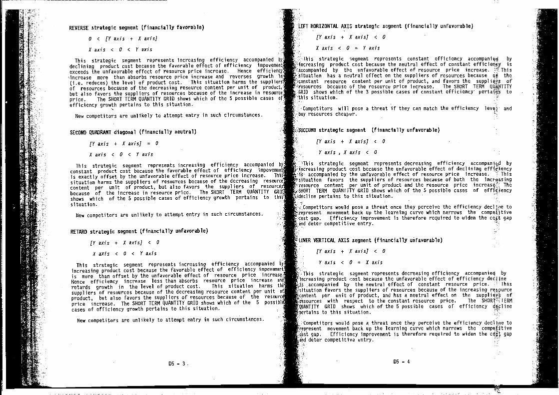
REVERSE strategic segment (financially favorable)
o < [V axis + X axis]
X axis < 0 < V axis
This strategic segment represents increasing efficiency accompanieddeclining product cost because the favorable effect of efficiency impovemelexceeds the unfavorable effect of resource price Increase. Hence efficieru
Increase more than absorbs resource price increase and reverses growth(i.e. reduces) the level of product cost. This situation harms the supplirof resources because of the decreasing resource content per unit of producibut also favors the suppliers of resources because of the increase in resounprice. The SHORT TERM QUANTITY GRID shows which of the 5 possible casesefficiency growth pertains to this situation.
New competitors are unlikely to attempt entry in such circumstances.
SECOND QUADRANT diagonal (financially neutral)
(Y axis + X axis] = 0
X axis C 0 < Y axis
This strategic segment represents increasing efficiency accompanied L,
constant product cost because the favorable effect of efficiency impoverneni
is exactly offset by the unfavorable effect of resource price increase. ThU
situation harms the suppliers of resources because of the decreasingcontent per unit of product, but also favors the suppliers of resobecause of the increase in resource price. The SHORT TERM QUANTITY G
shows which of the 5 possible cases of efficiency growth pertains tosituation.
New competitors are unlikely to attempt entry in such circumstances.
RETARD strategic segment (financially unfavorable)
(V axis + X axis] C 0
Kaxis < 0 < Vaxis
This strategic segment represents increasing efficiency accompanied b,
increasing product cost because the favorable effect of efficiency impoveeenis more than offset by the unfavorable effect of resource price increaseHence efficiency increase less than absorbs resource price increase a
retards growth in the level of product cost. This situation harmssuppliers of resources because of the decreasing resource content per unitproduct, but also favors the suppliers of resources because of the resourc
price increase. The SHORT TERM QUANTITY GRID shows which of the S possibl.cases of efficiency growth pertains to this situation.
New competitors are unlikely to attempt entry in such circumstances.
05 — 3
I:1
I
lEFT HORIZONTAL AXIS strategic segment (financially unfavorable)
This strategic egment represents constant efficiency accompaniqq byincreasing product cost because the neutral effect of constant efficierity is
companied by the unfavorable effect of resource price increase. Thistion has a neutral effect on the suppliers of resources because of thetnt resource content per unit of product, and favors the of
because of the resource price increase. The SHORT TERM
shows which of the 3 possible cases of constant efficiency pertaIns tothis situation.
Competitors will pose a threat if they can match the efficiency level andbuy resources cheaper.
strategic segment (financially unfavorable)
(Y axis + X axis] < 0
Y axis , X axis < 0
strategic segment represents decreasing efficiency accompanied byicreasing product cost because the unfavorable effect of declining
accompanied by the unfavorable effect of resource price increase. Thisituation favors the suppliers of resources because of both the
'eseurce content per unit of product and the resource price The)RT TERM QUANTITY GRID shows which of the 5 possible cases of effidency
!cline pertains to this situation.
Competitors would pose a threat once they perceive the efficiency declfne tomovement back up the learning curve which narrows the
cest gap. Efficiency improvement is therefore required to widen the gapdeter competitive entry.
LOWER VERTICAL AXIS segment (financially unfavorable)
(V axis + X axis] < 0
strategic segment represents decreasing efficiency accompanied byincreasing product cost because the unfavorable effect of efficiency declineis accompanied by the neutral effect of constant resource price. Thissituation favors the suppliers of resources because of the increasing respurce
per unit of product, and has a neutral effect on the ofesources with respect to the constant resource price. The SHORF TERMJANTITY GRID shows which of the 5 possible cases of efficiency
r.'taths to this situation.
* Competitors would pose a threat once they perceive the efficiency decliiie towesent movement back up the learning curve which narrows the compe,Utive
)st gap. Efficiency improvement is therefore required to widen the cqfl gapdeter competitive entry.
D5 — 4
(V axis + X axis] < 0
Xaxis < 0 = Vaxis
V axis < 0 = X axis
I
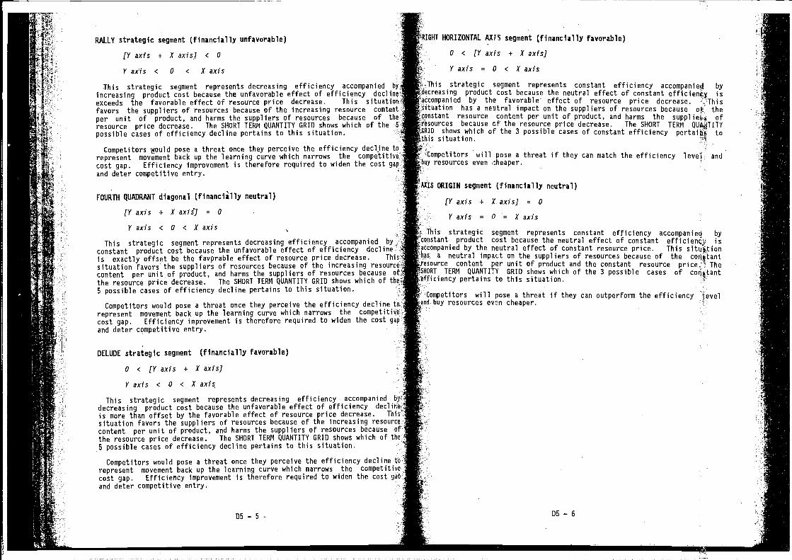
RALLY strategic segment (financially unfavorable)
axis + X axis] < 0
Yaxis < 0 < Xaxis
This strategic segment represents decreasing efficiency accompaniedincreasing product cost because the unfavorable effect of efficiencyexceeds the favorable effect of resource price decrease. This situatifavors the suppliers of resources because of the increasing resource contenper unit of product, and harms the suppliers of resources because of thresource price decrease. The SHORT TERM QUANTITY GRID shows which of thepossible cases of efficiency decline pertains to this situation.
Competitors Mould pose a threat once they perceive the efficiency decl.ine torepresent movement back up the learning curve which narrows the competiticost gap. Efficiency improvement is therefore required to widen the cost gapand deter competitive entry.
FOURTH QUADRANT diagonal (financlilly neutral)
(Yaxis + Xaxis'] = 0
Y axis c 0 < X axis
This strategic segment represents decreasing efficiency accompanied by
constant product cost because the unfavorable effect of efficiency declineis exactly offset be the favprable effect of resource price decrease, Thissituation favors the suppliers of resources because of the increasing resourcecontent per unit of product, and harms the suppliers of resources because of
the resource price decrease. The SHORT TERM QUANTITY GRID shows which of th5 possible cases of efficiency decline pertains to this situation.
Competitors would pose a threat once they perceive the efficiency declinerepresent movement back up the learning curve which narrows the competitivecost gap. Efficiency improvement is therefore required to widen the cost gapand deter competitive entry.
DELUDE strategic segment (financially favorable)
0 c (Yaxis + Xaxis]
Y axis < 0 c X axis
This strategic segment represents decreasing efficiency accompanieddecreasing product cost because the unfavorable effect of efficiency decliris more than offset by the favorable effect of resource price decrease. TLsituation favors the suppliers of resources because of the increasing resouncontent per unit of product, and harms the suppliers of resources becausethe resource price decrease. The SHORT TERM QUANTITY GRID shows which of5 possible cases of efficiency decline pertains to this situation.
Competitors would pose a threat once they perceive the efficiency declinerepresent movement back up the learning curve which narrows the competitircost gap. Efficiency improvement is therefore required to widen the costand deter competitive entry.
D5 — 5
IGHT HORIZONTAL AXIS segment (financially favorable)
V axis = 0 < X axis.
This strategic segment represents constant efficiency accompanied bydecreasing product cost because the neutral effect of constant isaccompanied by the favorable effect of resource price decrease.situation has a neutral impact on the suppliers of resources because of the-enstant resource content per unit of product, and harms the supplieiss ofesources because r.f the resource price decrease. The SHORT TERM QUAHTITYRID shows which of the 3 possible cases of constant efficiency to
situation.
uuv#ctitors will pose a threat if they can match the efficiency level andnay resources even
V axis = 0 A' axis
This strategic segment represents constant efficiency accompanied byConstant product cost because the neutral effect of constant isaccompanied by the neutral effect of constant resource price. This siti4tion
a neutral impact on the suppliers of resources because of the coriflantnurce content per unit of product and the constant resource price. TheiT TERM QUANTITY GRID shows which of the 3 possible cases of
pertains to this situation.
Competitors will pose a threat if they can outperform the efficiency ievel.1 buy resources cheaper.
D5 — 6
.4
0 c (V axis + A' axis]
ORIGIN segment (financially neutral)
(V axis + A' axis] = 0
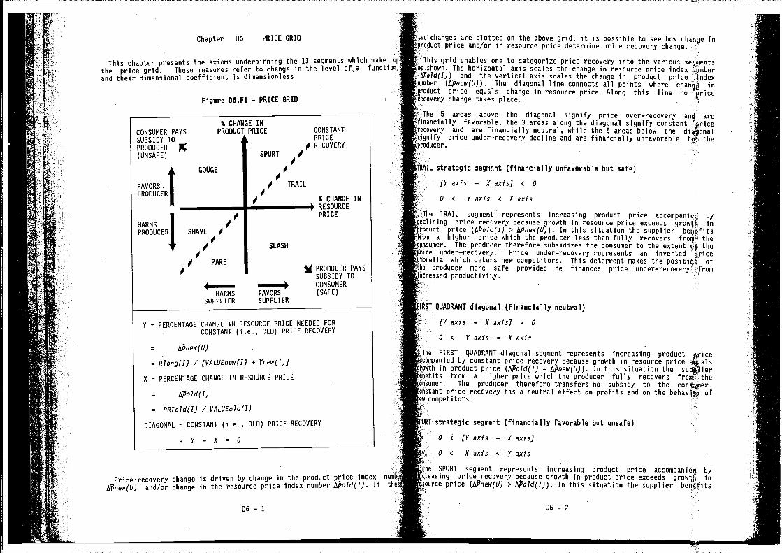
Chapter D6 PRICE GRID
This chapter presents the axioms uiiderpinning the 13 segments which make
the price grid. These measures refer to change in the level of, aand their dimensional coefficient is dimensionless.
Figure D6.Fl - PRICE GRID
Pricerecovery change is driven by change in the product price index nuni..
tsPnew(U) and/or change in the resource price index number APoJd(I). If
D6 - 1
s grid enables one to categorize price recovery into the various'n. The horizontal axis scales the change in resource price index
old(I)) and the vertical axis scales the change in product priceber (APnew(U)). The diagonal line connects all points where changQ induct price equals change in resource price. Along this line no Qriceavery change takes place. -
'e 5 areas above the diagonal signify price over—recovery and arencially favorable, the 3 areas along the diagonal signify constantvery and are financially neutral, while the 5 areas below the
price under—recovery decline and are financially unfavorable tw theoducer.
e TRAIL segment represents increasing product price accompanie4 bylining price recovery because growth in resource price exceeds induct price (lsPolci(T) > APnew(U)). In this situation the suppliero a higher price which the producer less than fully recovers from2 thesumer. The produ:er therefore subsidizes the consumer to the extent the
under—recovery. Price under—recovery represents an inverted priceolla which deters new competitors. This deterrent makes the ofproducer more safe provided he finances price under—recovery::from
creased productivity.
QUADRANT diagonal (financially neutral)
(Y axis — X axis) = 0
o < Yaxis = Xaxis
ie FIRST QUADRANT diagonal segment represents increasing product price)mpanied by constant price recovery because growth in resource price eqpals
Dwth in product price = In this situation thenefits from a higher price which the producer fully recovers from: the
sumer. The producer therefore transfers no subsidy to the cons)aoer.itant price recovery has a neutral effect on profits and on the ofcompetitors.
I strategic segment (financially favorable but unsafe)
0 < [V axis —. X axis]
o < Xaxis < Vaxis
SPURT segment represents increasing product price byprice recovery because growth in product price exceeds growth in
price > In this situation the supplier benpfits
D6 — 2
changes are plotted on the above grid, it is possible to see how chatwe tnduct price and/or in resource price determine price recovery change.
strategic segmnnt (financially unfavorable but safe)
[V axis — X axis] < 0
0 < Vaxis < Xaxis
% CHANGE INCONSUMER PAYS PRODUCT PRICE CONSTANT
SUBSIDY TO PRICE
PRODUCER p4 RECOVERY
(UNSAFE) SPURT p4
GOUGE
p4 TRAIL
PRODUCER p4
% CHANGE INRESOURCE
PRICE
HARMS p4
PRODUCER SHAVE
p4
0SLASH
PARE
0PRODUCER PAYSSUBSIDY TO
4CONSUMER
HARMS FAVORS (SAFE)SUPPLIER SUPPLIER
Y = PERCENTAGE CHANGE IN RESOURCE PRICE NEEDED FORCONSTANT (i.e., OLD) PRICE RECOVERY
= AThsew(U)
= Rlong(I) / [VALUEPeW(I) + Ynew(I)]
X = PERCENTAGE CHANGE IN RESOURCE PRICE
=
= PRIold(I) / VALUEoJd(I)
DIAGONAL = CONSTANT (i.e., OLD) PRICE RECOVERY
=y—x=o
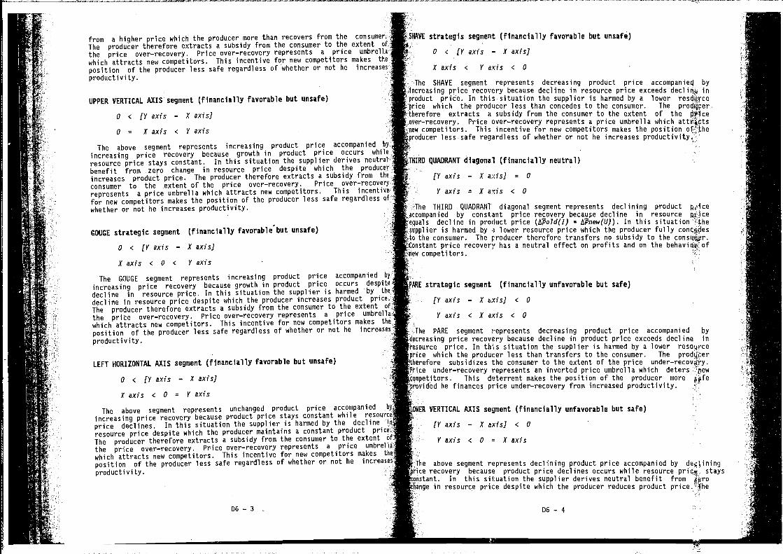
from a higher price which the producer more than recovers from theThe producer therefore extracts a subsidy from the consumer to the extentthe price over—recovery. Price over—recovery represents a price umbrell
which attracts new competitors. This incentive for new competitors makes t,position of the producer less safe regardless of whether or not he increase.
productivity.
UPPER VERTICAL AXIS segment (financially favorable but unsafe)
o < (Y axis — X axis]
o = Kaxis < Yaxis
The above segment represents increasing product price accompanied
increasing price recovery because growth in product price occurs while
resource price stays constant. In this situation the supplier derives neutralbenefit from zero change in resource price despite which the producer
increases product price. The producer therefore extracts a subsidy from the
consumer to the extent of the price over—recovery. Price over—recovery
represents a price umbrella which attracts new competitors. This incentivefor new competitors makes the position of the producer less safe regardless ef-iwhether or not he increases productivity.
GOUGE strategic segment (financially favorable but unsafe)
o < (Y axis — X axis]
X axis < 0 < Y axis
The GOUGE segment represents increasing product price accompanied by
increasing price recovery because growth in product price occurs despite
decline in resource price. In this situation the supplier is harmed by
decline in resource price despite which the producer increases product price.:The producer therefore extracts a subsidy from the consumer to the extent oh
the price over—recovery. Price over—recovery represents a price umbrell.
which attracts new competitors. This incentive for new competitors makes the
position of the producer less safe regardless of whether or not he increases
productivity.
LEFT HORIZONTAL AXIS segment (financially favorable but unsafe)
o < [Y axis — X axis]
X axis < 0 = Y axis
The above segment represents unchanged product price accompaniedincreasing price recovery because product price stays constant while resouri
price declines. In this situation the supplier is harmed by the declineresource price despite which the producer maintains a constant product prY
The producer therefore extracts a subsidy from the consumer to the extentthe price over—recovery. Price over—recovery represents a price umbrel
which attracts new competitors. This incentive for new competitors makes ti
position of the producer less safe regardless of whether or not he increas'
productivity.
DO — 3
The SHAVE segment represents decreasing product price accompanieØ byincreasing price recovery because decline in resource price exceeds inproduct price. In this situation the supplier is harmed by a lowerprice which the producer less than concedes to the consumer. The proelqcer
extracts a subsidy from the consumer to the extent of the TWice-——recovery. Price over—recovery represents a price umbrella which attr*cts
competitors. This incentive for new competitors makes the positionof whether or not he increases productivity.
The THIRD QUADRANT diagonal segment represents declining productaccompanied by constant price recovery because decline in resource pHceequals decline in product price (APold(I) = LtPnew(U)). In this situation -tesupplier is harmed by -e lower resource price which the producer fully concrijieso the consumer. The producer therefore transfers no subsidy to the consqür.onstant price recovery has a neutral effect on profits and on the
competitors.
PARE strategic segment (financially unfavorable but safe)
(Y axis — X axis] < 0
Y axis C X axis < 0
The PARE segment represents decreasing product price accompanied bycreasing price recovery because decline in product price exceeds decline in
esource price. In this situation the supplier is harmed by a lower resdurcerice which the producer less than transfers to the consumer. Theerefore subsidizes the consumer to the extent of the priceice under—recovery represents an inverted price umbrella which deterswtitors. This deterrent makes the position of the producer more
he finances price under—recovery from increased productivity.
_..!R VERTICAL AXIS segment (financially unfavorable but safe)
(Yaxis — Xaxis] C 0
Y axis < 0 = X axis
lie above segment represents declining product price accompanied by declininga recovery because product price declines occurs while resource price stays
estant. In this situation the supplier derives neutral benefit from flroange in resource price despite which the producer reduces product price:lhe
DO — 4
strategis segment (financially favorable but unsafe)
0 < (V axis — X axis]
X axis < V axis < 0
QUADRANT diagonal (financially neutral)
(V axis — X axis] = 0
Y axis = X aris C 0
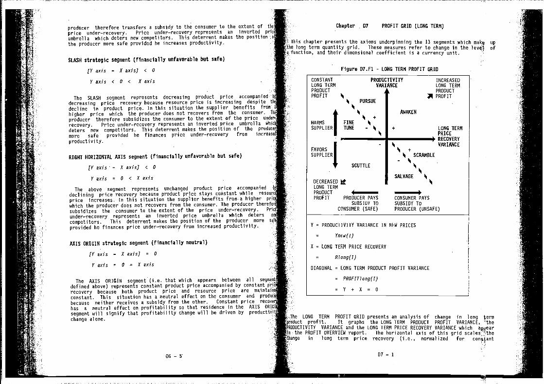
producer therefore transfers a subsidy to the consumer to the extent ofprice under—recovery. Price under—recovery represents an inverted priumbrella which deters new competitors. This deterrent makes the positionthe producer more safe provided he increases productivity.
SLASH strategic segment (financially unfavorable but safe)
(Y axis — X axis] < 0
Yaxis < 0 < Xaxis -
The SLASH segment represents decreasing product price accompanied
decreasing price recovery because resource price is increasing despitedecline in product price. In this situation the supplier benefitshigher price which the producer does not recovers from the consumer
producer therefore subsidizes the consumer to the extent of the price L.
recovery. Price under—recovery represents an inverted price umbrelladeters new competitors. This deterrent makes the position of the produce
more safe provided he finances price under—recovery from Increase
productivity.
RIGHT HORIZONTAL AXIS segment (financially unfavorable but safe)
[Y axis — X axis] < 0
Y axis = 0 < X axis
The above segment represents unchanged product price accompanied
declining price recovery because product price stays constant while reseurt
price increases. In this situation the supplier benefits from a higher pr4
which the producer does not recovers from the consumer. The producer theresubsidizes the consumer to the extent of the price under—recovery.under—recovery represents an inverted price umbrella which deterscompetitors. This deterrent makes the position of the producer more
provided he finances price under—recovery from increased productivity.
AXIS ORIGIN strategic segment (financially neutral)
jY axis — K axis] = 0
V axis = 0 = K axis
The AXIS ORIGIN segment (i.e. that which appears between all segme
defined above) represents constant product price accompanied by constantrecovery because both product price and resource price are maintaiconstant. This situation has a neutral effect on the consumer and produc'
because neither receives a subsidy from the other, Constant price recove
has a neutral effect on profitability so that residence in the AXIS ORI
segment will signify that profitability change will be driven by productichange alone.
Chapter D7 PROFIT GRID (LONG TERM)
This chapter presents the axioms underpinning the 13 segments which mak. uplong term quantity grid. These measures refer to change in the leve of
a function, and their dimensional coefficient is a currency unit.
The LONG TERM PROFIT GRID presents an analysis of change in long term"ict profit. It graphs the LONG TERM PRODUCT PROFIT VARIANCE,
CTIVITY VARIANCE and the LONG TERM PRICE RECOVERY VARIANCE whichthe PROFIT OVERVIEW report. The horizontal axis of this grid
iange in long term price recovery (i.e., normalized for
D7 — 1
Figure D7.F1 - LONG TERM PROFIT GRID
PRODUCTIVITYVARIANCE
PURSUE
AWAKEN
+FINETUNE
CONSTANTLONG TERMPRODUCT
PROFIT
HARMS
SUPPLIER
FAVORS
SUPPLIER
DECREASEDLONG TERMPRODUCT
PROFIT
INCREASEDLONG TERMPRODUCT
$ PROFIT
LONG TERMPRICERECOVERYVARIANCE
SCUTTLE
PROOUCER PAYSSUBSIDY TO
CONSUMER (SAFE)
sq
- SCRAMBLE
SALVAGE
CONSUMER PAYSSUBSIDY TOPRODUCER (UNSAFE)
F
k
L
Y = PROOUCTIVITY VARIANCE IN NEW PRICES
= yn&w(r)
X = LONG TERM PRICE RECOVERY
= Rlong(I)
DIAGONAL = LONG TERM PRODUCT PROFIT VARIANCE
= PROFIT7ong(I)
=Y+X=O
06 —
productivity), and the vertical axis scales the change in productivity. Bothaxes employ the same numerical scale. The diagonal line represents constantlong term product profit because it connects all points where the change inproductivity is exactly offset by an opposite change in long term pricerecovery normalized for constant productivity.
Starting with the AWAKEN segment, and proceeding in anti—clockwise order,the meaning of each of the above 13 case segments is defined below. Thenames of six case segments which do not occur along axes or the diagonal areintended to characterize typical •strategic reponses rather than rigidprescriptions. They do not relate to the short term and must be qualifiedshould any compelling contrary considerations be relevant.
AWAKEN strategic segment (financially favorable and partly unsafe)
0 < [Yaxis + Xaxis]
- 0 < Y axis , X axis
This strategic segment represents increasing productivity accompanied by
increasing long term product profit because price over—recovery also takesplace. This situation harms the suppliers of resources because of thedecreasing resource content per unit of product. It also harms the consumerbecause he pays to the producer a subsidy equivalent to the price over—recovery. The QUANTITY and PRODUCTIVITY GRIDS show which of the 5 possiblecases of productivity growth pertains to this situation, and the PRICE GRID
shows which of the 5 possible cases of price over—recovery pertains to thissituation.
Awaken a business in this strategic segment. The combination of increasinglong term product profit and umbrella pricing could trigger the entry ofcompetitors. However, even if competitive entry completely eliminates theprice umbrella, this business would reflect lower, but still positive,in long term product profit on account of productivity gain. The danger isnot as severe here as it is in the Scramble strategic segment.
UPPER VERTICAL AXIS strategic segment (financially favorable and safe)
o < [V axis + XaxisJ
o = Xaxis < Yaxis
This strategic segment represents increasing productivity accompanied byincreasing long term product profit because constant long term price recoverytakes place. This situation harms the suppliers of resources because ofdecreasing resource content per unit of product. It is also neutral toconsumer and producer because neither pays a subsidy to the other. The-QUANTITY and PRODUCTIVITY GRIDS show which of the S possible cases efproductivity growth pertains to this situation, and the PRICE GRID shows whichof the 3 possible cases of constant price recovery pertains to this situation,
In the UPPER VERTICAL AXIS strategic segment the entire productivity pie is -
retained by the producer to improve profitability.
D7 — 2
PURSUE strategic Legment (financially favorable and safe)
0 < [V axis + Xaxis]
Xaxis < 0 < Vaxis
This strategic segment represents increasing productivity accompapied byIncreasing long term product profit because productivity impovement' exceedsprice under—recovery.. This situation harms the suppliers of Vesourcesbecause of the decreasing resource content per unit of product. 'It alsofavors the consumer because he receives from the producer a subsidy qqpivalentto the price under—recovery. The QUANTITY and PRODUCTIVITY GRIDS whichof the S possible cases of productivity growth pertains to this situation, andthe PRICE GRID shows which of the S possible cases of price underrecovery
¾ perthins to this situation.
In the PURSUE strategic segment the productivity pie is shared befween theproducer and the consumer. -
Pursue the same path in a business in this strategic segment. This is themost favored of segments because productivity gain is being used td financethe creation of an inverted price umbrella consistent with longterm product profit. Despite improving long term product profit, newcompetitors are unlikely to attempt entry in the face of an invertüd priceumbrella and the productivity growth registered by the business.
SECOND QUADRANT diagonal (financially neutral and safe)
[V axis + Xaxis] = 0
Xaxis < 0 < Vaxis
This strategic segment represents increasing productivity byconstant long term product profit because productivity impovement is:: exactlyoffset by price under—recovery. This situation harms the suppljers ofresources because of the decreasing resource content per unit of product. It
- also favors the consumer because he receives from the producerequivalent to price under—recovery. The QUANTITY and PRODUCTIVITY GRIDSshow which of the 5 possible cases of productivity growth pertains -to thissituation, and the PRICE GRID shows which of the 5 possible cases ef priceunder—recovery pertains to this situation.
In the SECOND QUADRANT diagonal strategic segment the entire productivitypie is transferred by the producer to the consumer by way of pricj' under—
j.recovery.
FINETUNE strategic segment (financially unfavorable and safe)
[V axis + X axis] < 0
Xaxis < 0 .c Yaxis
This strategic segment represents increasing productivity bydecreasing long term product profit because productivity isexceeded by price under—recovery. This situation harms the supp[fers of
because of the decreasing resource content per unit of Italso favors the consumer because he receives from the producer
It
07 — 3
In the FINETUNE strategic segment a benefit which is more than the entireproductivity pie is transferred from the producer to the consumer. Thproducer dilutes profitability to the extent of the decline in long tL.product profit to finance the excess of the benefit over the productivity ph
Fine—Tune a business in this strategic segment. It has the samegrowth and inverted price umbrella characteristics as the Pursue stratisegment, but the balance between them requires fine—tuning. This can beeither by reducing the extent of the negative long term price recovery orfurther inversion of the price umbrella, provided it is more then offsetfurther increases in productivity growth.
LEFT HORIZONTAL AXIS strategic segment (financially unfavorable and safe)
(V axis + X axis) < 0
X axis < 0 = Y axis
This strategic segment represents constant productivity accompanieddecreasing long term product profit because price under—recovery takes plaiThis situation has a neutral impact on the suppliers of resources becausethe constant resource content per unit of product. It is also favorsconsumer because he receives from the producer a subsidy equal to the prunder—recovery. The QUANTITY and PRODUCTIVITY GRIDS show which of thepossible cases of constant productivity pertains to this situation, and U
PRICE GRID shows which of the 5 possible cases of price under—recoveipertains to this situation.
In the LEFT HORIZONTAL AXIS strategic segment there is no productivityto share between producer and consumer.
SCUTTLE strategic segment (financially unfavorable and partly unsafe)
(V axis + X axis) < 0
V axis , X axis < 0
This strategic segment represents decreasing productivity accompanieddecreasing long term product profit because price under—recovery also tplace. This situation favors the suppliers of resources because of tincreasing resource content per unit of product. It also favors the consun'because he receives from the producer a subsidy equivalent to the price underecovery. The QUANTITY and PRODUCTIVITY GRIDS show which of the 5 possibcases of productivity decline pertains to this situation, and the PRICE Ishows which of the 5 possible cases of price under—recovery pertains to tsituation.
In the SCUTTLE strategic segment there is no productivity pie to s:..between producer and consumer. Instead there is a productivity deficit.
Scuttle (i.e., abandon) a business in this strategic segment. Thistypically a dying business with high fixed cost which is unable to recover
D7 — 4 -
This strategic segment represents decreasing productivity accompaniej$ byecreasing long term product profit because constant long term priceekes place. This situation favors the suppliers of resources because oftheecreasing resource content per unit of product. It is also neutra toonsumer and producer because neither pays a subsidy to the other. The
and PRODUCTIVITY GRIDS show which of the S possible cases ofpreductivity decline pertains to this situation, and the PRICE GRIDwhich of the 3 possible cases of constant price recovery pertains to-4his
ion.
In the LOWER VERTICAL AXIS strategic segment there is no productivity piç toshare between producer and consumer. Instead there is a productivity
LVAGE strategic segment (financially unfavorable and unsafe)
(Y axis + X axis) < 0
Yaxis c 0 < Xaxis
This strategic segment represents decreasing productivity accompanigØ bydecreasing long term product profit because productivity decline exceeds pricever—recovery. This situation favors the suppliers of resources of:.a increasing resource content per unit of product. It also harms theDnsumer because he pays to the producer a subsidy equivalent to the pricever—recovery. The QUANTITY and PRODUCTIVITY GRIDS show which of 5
cases of productivity decline pertains to this situation,GRID shows which of the 5 possible cases of price over—recovery perUins
this situation.
the SALVAGE strategic segment there is no productivity pie to oAarebetween producer and consumer. Instead there is a productivity deficit. -
calvage a business in this strategic segment. Performance profit is:lining because productivity loss exceeds the price recovery gain creat.d by
umbrella pricing situation. Relief from dependence on umbrella isincentive to try to restore productivity levels and reversn the long eterm
roduct profit decline. The threat of newcomers entering under the pjiceis lower than in the next strategic segment.
DURTH QUADRANT diagonal (financially neutral and unsafe)
V axis C 0 < X axis
This strategic segment represents decreasing productivity byonstant long term product profit because productivity decline is
D7 — 5
a
equivalent to the price under—recovery. The QUANTITY and PRODUCTIVITY GRT'
show which of the 5 possible cases of productivity growth pertains to U
situation, and the PRICE GRID shows which of the 5 possible cases of p.
under—recovery pertains to this situation.
reduct price increase the full extent of the resource price increase to ghicht is exposed.
VERTICAL AXIS segment (financially unfavorable and partly unsafe)
(Y axis + X axis) < 0
V axis c 0 = X axis
(V axis + X dxis) = 0
offset by price over—recovery. This situation favors the suppliersresources because of the increasing resource content per unit of product.also harms the consumer because he pays to the producer a subsidy equivalrto the price over—recovery. The QUANTITY and PRODUCTIVITY GRIDS show whiof the 5 possible cases of productivity decline pertains to this situaticand the PRICE GRID shows which of the 5 possible cases of price over—recoverpertains to this situation.
In the FQURTH QUADRANT diagonal strategic segment there is no productivitpie to share between producer and consumer. Instead there is a producti.;deficit.
SCRAMBLE strategic segment (financially favorable and unsafe)
0 < (Y axis + X axis]
V axis < 0 < X axis
This strategic segment represents decreasing productivity accompaniedincreasing long term product profit because productivity decline is more t..offset by price over—recovery. This situation favors the suppliers o
resources because of the increasing resource content per unit of product. I
also harms the consumer because he pays to the producer a subsidy equivale-to the price over—recovery. The QUANTITY and PRODUCTIVITY GRIDS showof the 5 possible cases of productivity decline pertains to this situationand the PRICE GRID shows which of the 5 possible cases of price over—recoverpertains to this situation.
In the SCRAMBLE strategic segment there is no productivity pie tobetween producer and consumer. Instead there is a productivity deficit.
Scramble to protect a business in this strategic segment. Performance pis increasing because the umbrella pricing gain exceeds (and Ii
camouflages) productivity loss. The threat of new competitors is real becausof both umbrella pricing and increasing long term product profit. Furthermoreproductivity loss narrows the productivity gap between this business and tlow productivity levels of newcomers to the market. A quick turnaroundproductivity loss to gain is needed, since competitive erosion of theumbrella could transform this business from increasing to decreperformance profit.
RIGHT HORIZONTAL AXIS segment (financially favorable and unsafe)
0 < (Y axis + X axis]
Y axis = 0 C X axis
to share between producer and consumer.
5 ORIGIN segment (financially neutral)
(V axis + X axis] = 0
V axis = 0 = A' axis
This strategic soqment represents constant productivity accompanied byconstant long term product profit because constant price recovery takesThis situation has a neutral impact on the suppliers of resources becausi' of'ie constant, resource content per unit of product. It also has a
t on consumer and producer since neither pays a subsidy to the other,[Theand PRODUCTIVITY GRIDS show which of the 3 possible cases of
productivity pertains to this situation, and the PRICE GRID shows which otthe3 possible cases of constant long term price recovery pertains tosituation.
In the AXIS ORIGIN strategic segment there is no productivity pie to 4!arebetween producer and consumer.
The advanced reader will appreciate the grid rule on the following page,
D7 — 7
This strategic segment represents constant productivity accompanied b,
increasing long term product profit because price over—recovery takes placeThis situation has a neutral impact on the suppliers of resources because o
the constant resource content per unit of product. It is also harms tkconsumer because he pays to the producer a subsidy equal to the price overecovery. The QUANTITY and PRODUCTIVITY GRIDS show which of the 3 possi'cases of constant productivity pertains to thi situation, and the PRICE G
shows which of the 5 possible cases of price over—recovery pertains to +
situation.• In the RIGHT HORIZONTAL AXIS strategic segment there is no productivity p1
D7 — 6
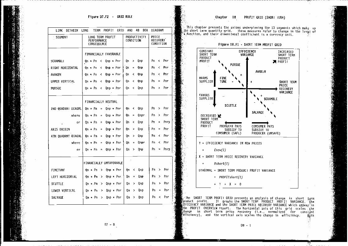
Figure D7.F2 - GRID RULE
LINK BETWEEN LONG TERM PROFIT GRID AND 48 BOX DIAGRAM
SEGMENT LONG TERM PROFITPERFORMANCE
CONSEQUENCE
PRODUCTIVITYCONDITION
PRICERECOVERYCONDITION
SCRAMBLE
RIGHT HORIZONTAL
AWAKEN
UPPER VERTICAL
PURSUE
FINANCIALLY FAVORABLE
Qn * Pn Qnp * Pnr
Qn * Pn < Qnp * Pnr
Qn * Pn < Qnp * Pnr
Qn * Pn < Qnp * Pnr
Qn * Pn < Qnp * Pnr
Qn > Qnp
Qn = Qnp
Qn < Qnp
Qn < Qnp
Qn < Qnp
Pn < Pnr
Pn < Pnr
Pn < Pnr
Pn = Pnr
Pn > Pnr
2ND QUADRNT DIAGNL
where
or
AXIS ORIGIN
4TH QUADRNT DIAGNL
where
or
FINANCIALLY NEUTRAL
Qn * Pn = Qnp * Pnr
Qn * Pn = Qnp * Pnr
Qn * Pn = Qnp * Pnr
Qn * Pn = Qnp * Pnr
Qn * Pn = Qnp * Pnr
Qn * Pn = Qnp * Pnr
Qn * Pn = Qnp * Pnr
Qn < Qnp
Qn = Qnpr
Qn < Qnp
Qn = Qnp
Qn > Qnp
Qn = Qnpr
Qn > qnp
Pn > Pnr
Pn > Pnr
Pn = Pnrp
Pn = Pnr
Pn < Pnr
Pn < Pnr
Pn = Pnrp
FINETUNE
LEFT HORIZONTAL
SCUTTLE
LOWER VERTICAL
SALVAGE
FINANCIALLY UNFAVORABLE
Qn * Pn > Qnp * Pnr
Qn * Pn > Qnp * Pnr
Qn *Pn > Qnp * Pnr
Qn * Pn > Qnp * Pnr
Qn * Pn > Qnp * Pnr
Qn < Qnp
Qn = Qnp
Qn > Qnp
Qn > Qnp
Qn > Qnp
Pn > Pnr
Pn > Pnr
Pn > Pnr
Pn = Pnr
Pn < Pnr
07 — 8
Chapter 08 PROFIT GRID (SHORT TERM)
This chapter presents the axioms underpinning the 13 segments which make upshort term quantity grid. These measures refer to change in the of
a function, and their dimensional coefficient is a currency unit.
Figure D8.F1 - SHORT TERM PROFIT GRID
The SHORT TERM PROFIT GRID presents an analysis of change in short)roduct profit. It graphs the SHORT TERM PRODUCT PROFIT VARIANCE, the
FICIENCY VARIANCE and the SHORT TERM PRICE RECOVERY VARIANCE whiche PROFIT OVERVIEW report. The horizontal axis of this grid scales (heange in short term price recovery (i.e., normalized for constant
and the vertical axis scales the change in efficiency.
08 — 1
CONSTANTSHORT TERMPRODUCT
PROF IT
EFFICIENCYVARIANCE
PURSUE
INCREASEDSHORT TERMPRODUCT
$ PROFIT
b1 +
FINE b1
TUNE -
AWAKEN
HARMS
SUPPLIER
FAVORS
SUPPLIER
+ SHORT TERMPRICE
+ RECOVERYVARIANCE
SCUTTLE
SCRAMBLE
'I,'
SALVAGEDECREASEDSHORT TERMPRODUCT
PROFIT PRODUCER PAYSSUBSIDY TO
CONSUMER (SAFE)
CONSUMER PAYSSUBSIDY TOPRODUCER (UNSAFE)
Y = EFFICIENCY VARIANCE IN NEW PRICES
= Enew(I)
X = SHORT TERM PRICE RECOVERY VARIANCE
= Rshort(I)
DIAGONAL SHORT TERM PRODUCT PROFIT VARIANCE
= PROFITshort(I)
= 'I + X = 0
axes employ the same numerical scale. The diagonal line represents constantshort term product profit because It connects all points where the change inefficiency Is exactly offset by an opposite change in short term price,recovery normalized for constant efficiency.
Starting with the AWAKEN segment, and proceeding in anti—clockwise order,the meaning of each of the above 13 case segments is defined below. Thenames of six case segments which do not occur along axes or the diagonal areintended to characterize typical strategic reponses rather than rigidprescriptions. They do not relate to the short term and must be qualifiedshould any compelling contrary considerations be relevant.
AWAKEN strategic segment (financially favorable and partly unsafe)
o < (Vax/s + lax/sfo < Vax/s , lax/s
This strategic segment represents increasing efficiency accompanied by
increasing short term product profit because price over—recovery also takesplace. This situation harms the suppliers of resources because of thedecreasing resource content per unit of product. It also harms the consumerbecause he pays to the producer a subsidy equivalent to the price oversrecovery. The SHORT TERM QUANTITY GRID shows which of the 5 possible casesof efficiency growth pertains to this situation, and the PRICE GRID shows'which of the 5 possible cases of price over—recovery pertains to thissituation.
Awaken a business in this strategic segment. The combination of increasingshort term product profit and umbrella pricing could trigger the entry of new
competitors. However, even if competitive entry completely eliminates theprice umbrella, this business would reflect lower, but still positive, changein short term product profit on account of efficiency gain. The danger isnot as severe here as it is in the Scramble strategic segment.
UPPER VERTICAL AXIS strategic segment (financially favorable and safe)
o < (V ax/s + I ax/sf
o = I ax/s c V ax/s
This strategic segment represents increasing efficiency accompanied by'increasing short term product profit because constant short term price-recovery takes place. This situation harms the suppliers of resourcesbecause of the decreasing resource content per unit of product. It is alsoneutral to consumer and producer because neither pays a subsidy to the other.The SHORT TERM QUANTITY GRID shows which of the 5 possible cases of efficiencrgrowth pertains to this situation, and the PRICE GRID shows which of the 3
possible cases of constant price recovery pertains to this situation.
In the UPPER VERTICAL AXIS strategic segment the entire efficiency pie isretained by the producer to improve profitability.
DR — 2
PURSUE strategic segment (financially favorable and safe)
0 < (Vax/s + lax/sflax/s < o < Yax/s -
This strategic segment represents increasing efficiency accompaniect by'increasing short term product profit because efficiency impovement exnedsprice under—recovery. This situation harms the suppliers of resoqgcesof the decreasing resource content per unit of product. It £lsofavors the consumer because he receives from the producer a subsidyto the price under—recovery. The SHORT TERM QUANTITY GRID shows which
of efficiency growth pertains to this situation, and thePRICE GRID shows which of the 5 possible cases of pricepartains to this situation.
In the PURSUE strategic segment the efficiency pie is shared between - kheproducer and the consumer.
Pursue the same path in a business in this strategic segment. This is ' themost favored of segments because efficiency gain is being used to finance thecreation of an inverted price umbrella consistent with increasing short Lrmproduct profit. Despite improving short term product profit, new'are unlikely to attempt entry in the face of an inverted price umbrellathe efficiency growth registered by the business.
SECOND QUADRANT diagonal (financially neutral and safe)
(Vax/s + lax/sf = 0
- lax/s < a < Vax/s
This strategic segment represents increasing efficiency accompanied by'constant short term product profit because efficiency impovement is exactly'offset by price under—recovery. This situation harms the suppliersresources because of the decreasing resource content per unit of product. Italso favors the consumer because he receives from the producer aeqoivalent to the price under—recovery. The SHORT TERM QUANTITY GRID shbwswhich of the 5 possible cases of efficiency growth pertains to this situatfçjai,'eod the PRICE GRID shows which of the S possible cases of price under—recoyfrypertains to this situation.
In the SECOND QUADRANT diagonal strategic segment the entire efficiency &etransferred by the producer to the consumer by way of price
FINETUNE strategic segment (financially unfavorable and safe)
(Vax/s + lax/sf C 0
I ax/s c 0 c V ax/s
This strategic segiaent represents increasing efficiency accompanied bydecreasing short term product profit because efficiency impovement isby price under—recovery. This situation harms the suppliers ofbecause of the decreasing resource content per unit of product. It aHofavors the consumer because he receives from the producer a subsidy equival'4jitto the price under—recovery. The SHORT TERM QUANTITY GRID shows which of
D8—3
5 possible cases of efficiency growth pertains to this situation, and the
PRICE GRID shows which of the S possible cases of price under—recoveypertains to this situation.
In the FINETUNE strategic segment a benefit which is more than the entirefficiency pie is transferred from the producer to the consumer. Th
producer dilutes profitability to the extent of the decline in short telproduct profit to finance the excess of the benefit over the efficiency pie.
Fine—Tune a business in this strategic segment. It has the same efficientgrowth and inverted price umbrella characteristics as the Pursue strategisegment, but the balance between them requires fine—tuning. This can be don
either by reducing the extent of the negative short term price recovery orfurther inversion of the price umbrella, provided it is more then offsetfurther increases in efficiency growth.
LEFT HORIZONTAL AXIS strategic segment (financially unfavorable and safe)
(V axis + Xaxisj < 0
X axis < 0 = V axis
This strategic segment represents constant efficiency accompanied hidecreasing short term product profit because price under—recovery takes place.This situation has a neutral impact on the suppliers of resources because of
the constant resource content per unit of product. It is also favors the
consumer because he receives from the producer a subsidy equal to theunder—recovery. The SHORT TERM QUANTITY GRID shows which of the 3 possiblecases of constant efficiency pertains to this situation, and the PRICE GRI
shows which of the 5 possible cases of price under—recovery pertains to thissituation.
In the LEFT HORIZONTAL AXIS strategic segment there is no efficiency pie to
share between producer and consumer.
SCUTTLE strategic segment (financially unfavorable and partly unsafe)
(Y axis + X axis] < 0
V axis , X axis < 0
This strategic segment represents decreasing efficiency accompanied by
decreasing short term product profit because price under—recovery also taketplace. This situation favors the suppliers of resources because ofincreasing resource content per unit of product. It also favors the consumtbecause he receives from the producer a subsidy equivalent to the pricerecovery. The SHORT TERM QUANTITY GRID shows which of the 5 possible cases
of efficiency decline pertains to this situation, and the PRICE GRID shewr
which of the 5 possible cases of price under—recovery pertains to thlcsituation.
In the SCUTTLE strategic segment there i.s no efficiency pie to share betweenproducer and consumer. Instead there is a efficiency deficit.
Scuttle (i.e., abandon) a business in this strategic segment. Thistypically a dying business with high fixed cost which is unable to recover hiproduct price increase the full extent of the resource price increase to which
DR — 4
dt is exposed.
LOWER VERTICAL AXIS segment (financially unfavorable and partly unsafe)
(V axis + X axis] < 0
V axis < C = X axis
This strategic segment represents decreasing efficiency accompaniq4 bydecreasing short term product profit because constant short term twicerecovery takes pluce. This situation favors the suppliers ofbecause of the increasing resource content per unit of product. It is 'alsoneutral to consumer and producer because neither pays a subsidy to the ojher.The SHORT TERM QUANTITY GRID shows which of the 5 possible cases ofdecline pertains to this situation, and the PRICE GRID shows which of 3possible cases of constant price recovery pertains to this situation.
In the LOWER VERTICAL AXIS strategic segment there is no efficiency toshare between producer and consumer. Instead there is a efficiency deficIt.
SALVAGE strategic segment (financially unfavorable and unsafe)
(V axis + X axis] c 0
Yaxis < 0 < Xaxis
This strategic segment represents decreasing efficiency accompanied bydecreasing short term product profit because efficiency decline exceedsrover_recovery. This situation favors the suppliers of resources ofthe increasing resource content per unit of product. It also harms theconsumer because he pays to the producer a subsidy equivalent to the pciceover—recovery. The SHORT TERM QUANTITY GRID shows which of the 5
cases of efficiency decline pertains to this situation, and the PRICEshows which of the 5 possible cases of price over—recovery pertains to thissituation.
In the SALVAGE strategic segment there is no efficiency pie to share betweenproducer and consumer. Instead there is an efficiency deficit.
Salvage a business in this strategic segment. Performance profit isdeclining because efficiency loss exceeds the price recovery gain by
'an umbrella pricing situation. Relief from dependence on umbrella prici4 isan incentive to try to restore efficiency levels and reverse the short termproduct profit decline. The threat of newcomers entering under theumbrella is lower than in the next strategic segment.
!OURTH QUADRANT diagonal (financially neutral and unsafe)
(Vaxis + = 0
V axis < 0 c A' axis
This strategic segment represents decreasing efficiency accompanied byconstant short term product profit because efficiency decline isoffset by price over—recovery. This situation favors the ofresources because of the increasing resource content per unit of It
F;!
08 — 5
S
also harms the consumer because he pays to the producer a subsidy equivato the price over—recovery. The SHORT TERM QUANTITY GRIO shows which of5 possible cases of efficiency decline pertains to this situation, andPRICE GRIO shows which of the 5 possible cases of price over—recovery pertato this situation.
In the FOURTH QUAORANT diagonal strategic segment there is no efficienc'to share between producer and consumer.. Instead there is a efficideficit.
SCRAMBLE strategic segment (financially favorable and unsafe)
0 < (Y axis + X axis]
Yaxis < 0 < Xaxis
This strategic segment represents decreasing efficiency accompaniedincreasing short term product profit because efficiency decline is more U.
offset by price over—recovery. This situation favors the suppliersresources because of the increasing resource content per unit of product.also harms the consumer because he pays to the producer a subsidyto the price over—recovery. The SHORT. TERM QUANTITY GRIO shows which of5 possible cases of efficiency decline pertains to this situation, andPRICE GRIO shows which of the 5 possible cases of price over—recovery pertato this situation.
In the SCRAMBLE strategic segment there is no efficiency pie tobetween producer and consumer. Instead there is a efficiency deficit.
Scramble to protect a business in this strategic segment. Performance pis increasing because the umbrella pricing gain exceeds (and h_,..
camouflages) efficiency loss. The threat of new competitors is real becauseboth umbrella pricing and increasing short term product profit. FurthermorEefficiency loss narrows the efficiency gap between this business and theefficiency levels of newcomers to the market. A quick turnaround fiefficiency loss to gain is needed, since competitive erosion of the p
umbrella could transform this business from increasing toperformance profit.
RIGHT HORIZONTAL AXIS segment (financially favorable and unsafe)
0 < (Y axis + X axis]
Y axis = 0 c X axis
This strategic segment represents constant efficiency accompaniedincreasing short term product profit because price over—recovery takes plarThis situation has a neutral impact on the suppliers of resources becausethe constant resource content per unit of product. It is also harmsconsumer because he pays to the producer a subsidy equal to the price e
recovery. The SHORT TERM QUANTITY GRIO shows which of the 3 possible c
of constant efficiency pertains to thi situation, and the PRICE CR10 s
which of the 5 possible cases of price over—recovery pertains to tsituation.
In the RIGHT HORIZONTAL AXIS strategic segment there is no efficiency pieshare between producer and consumer.
08 — 6
i,d5 strategic segment represents constant efficiency accompanied byshort term product profit because constant price recovery takes
3ce. This situation has a neutral impact on the suppliers ofresource content per unit of product. It also has a
eutral impact on consumer and producer since neither pays a subsidy to tháther. The SHORT TERM QUANTITY CR10 shows which of the 3 possible cases of'stant efficiency pertcins to this situation, and the PRICE CR10 shows whichthe 3 possible cases of constant short term price recovery pertains toLuat ion.
In the AXIS ORIGIN strategic segment there is no efficiency pie to shareetween producer and consumer.
The advanced reader will appreciate the grid rule on the next page.
08 — 7
ORIGIN segment (financially neutral)
[Yaxis + Xaxis] = 0
Y axis = 0 = I axis
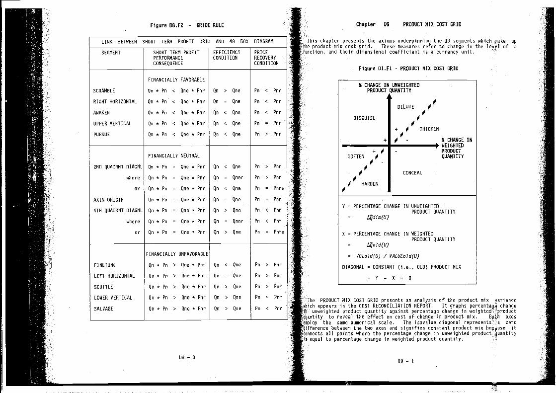
The PRODUCT MIX COST GRID presents an analysis of the product mix yariancewhich appears in the COST RECONCILIATION REPORT. It graphs changelii unweighted product quantity against percentage change inqaantity to reveal the effect on cost of change in product mix. Bpjh axesemploy the same numerical scale. The isovalue diagonal represents zerodifference betweei the two axes and signifies constant product mix beç4use itcannects all points where the percentage change in unweighted productis equal to percentage change in weighted product quantity.
LINK 8ETWEEN SHORT TERM PROFIT GRID AND 48 BOX DIAGRAM
Figure D8.F2 - GRIDE RULE Chapter D9 PRODUCT MIX COST GRID
This chapter presents the axioms underpinning the 13 segments which make upproduct mix cost grid. These measures refer to change in the of a
fanction, and their dimensional coefficient is a currency unit.
Figure D1.F1 - PRODUCT MIX COST GRID
% CHANGE IN UMWEIGHTEDPRODUCT QUANTITY
DISGUISE
DILUTE
THICKEN
SEGMENT SHORT TERM PROFITPERFORMANCE
CONSEQUENCE
EFFICIENCYCONDITION
PRICERECOVERY
CONDITION
SCRAMBLE
RIGHT HORIZONTAL
AWAKEN
UPPER VERTICAL
PURSUE
FINANCIALLY FAVORABLE
Qn * Pn < Qne * Pnr
Qn * Pn < Qne * Pnr
Qn * Pn c Qne * Pnr
Qn * Pn < Qne * Pnr
Qn * Pn < Qne * Pnr
Qn > Qne
Qn = Qne
Qn c Qne
Qn C Qne
Qn C Qne
Pn < Pnr
Pn < Pnr
Pn < Pnr
Pn = Pnr
Pn > Pnr
2ND QUADRNT DIAGNL
where
or
AXISORIGIN
4TH QUADRNT DIAGNL
where
or
FINANCIALLY NEUTRAL
qn * Pn = Qne * Pnr
Qn * Pn = Qne * Pnr
Qn*Pn = Qne*Pnr
Qn*Pn=Qne*Pnr
Qn * Pn = Qne * Pnr
Qn*Pn = Qne*Pnr
Qn*Pn = Qne*Pnr
Qn < Qne
Qn = Qner
Qn < Qne
Qn=Qne
Qn > Qne
Qn = Qner
Qn > Qne
Pn > Pnr
Pn > Pnr
Pn = Pnre
Pn=PnrPn < Pnr
Pn < Pnr
Pn = Pnre
FINETUNE
LEFT HORIZONTAL
SCUTTLE
LOWER VERTICAL
SALVAGE
FINANCIALLY UNFAVORABLE
Qn * Pn > Qne * Pnr
Qn * Pn > Qne * Pnr
Qn*Pn>Qne*Pnr
Qn * Pn > Qne * Pnr
Qn*Pn > Qne*Pnr
Qn < Qne
Qn = Qne
Qn>Qne
Qn > Qne
Qn > Qne
Pn > Pnr
Pn > Pnr
Pn>PnrPn = Per
Pn C Pnr
1-+
'4
% CHANGE IN4 WEIGHTED
PRODUCTQUANTITYSOFTEN
jJ'4
HARDEN
CONCEAL
'4
Y = PERCENTAGE CHANGE IN UNWEIGHTEDPRODUCT QUANTITY
IN WEIGHTEDPRODUCT QUANTITY
= PERCENTAGE CHANGE
=
= VOL0!d(LJ) / VALUEoJdflJ)
DIAGONAL = CONSTANT (i.e., OLD) PRODUCT MIX
= Y — X = 0
D8 — 8D9 — 1
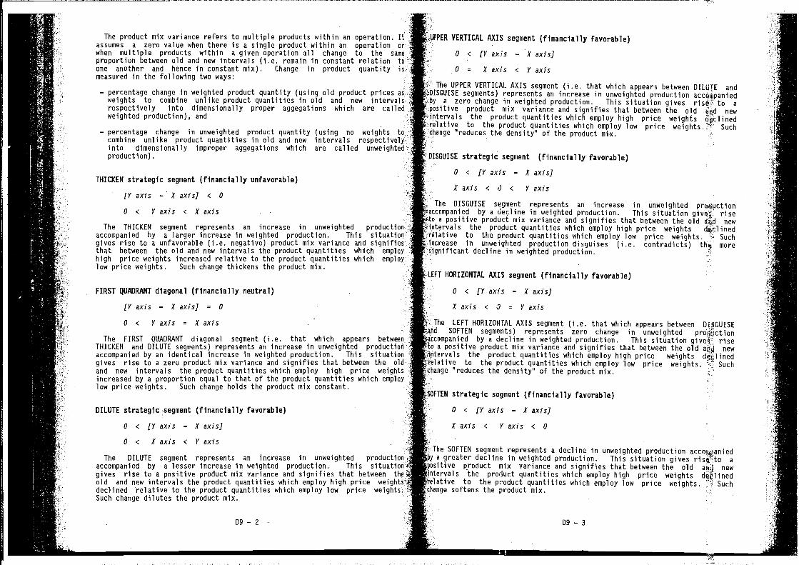
S
The product mix variance refers to multiple products within an operation. Itassumes a zero value when there is a single product within an operation orwhen multiple products within a given operation all change to the same -
proportion between old and new intervals (i.e. remain in constant relation toone another and hence in constant mix). Change in product quantity ismeasured in the following two ways:
— percentage change in weighted product quantity (using old product prices asweights to combine unlike product quantities in old and new intervalsrespectively into dimensionally proper aggegations which are calladweighted production), and
— percentage change in unweighted product quantity (using no weights tocombine unlike product quantities in old and new intervals respectivelyinto dimensionally improper aggegations which are called unweightedproduction).
THICKEN strategic segment (financially unfavorable)
[Yaxis — Xaxis] < 0
o < Yaxis < Xaxis
The THICKEN segment represents an increase in unweighted productionaccompanied by a larger increase in weighted production. This situationgives rise to a unfavorable (i.e. negative) product mix variance and signifiesthat between the old and new intervals the product quantities which employhigh price weights increased relative to the product quantities which employlow price weights. Such change thickens the product mix.
FIRST QUADRANT diagonal (financially neutral)
[V axis — Xaxis] = 0
o < V axis = K axis
The FIRST QUADRANT diagonal segment (i.e. that which appears betweenTHICKEN and DILUTE segments) represents an increase in unweighted productionaccompanied by an identical increase in weighted production. This situationgives rise to a zero product mix variance and signifies that between the oldand new intervals the product quantities which employ high price weightsincreased by a proportion equal to that of the product quantities which employlow price weights. Such change holds the product mix constant.
DILUTE strategic segment (financially favorable)
o < [V axis — K axis]
o < Xaxis < Yaxis
The DILUTE segment represents an increase in unweighted productionaccompanied by a lesser increase in weighted production. This situation',gives rise to a positive product mix variance and signifies that between thaiold and new intervals the product quantities which employ high pricedeclined relative to the product quantities which employ low price weights.Such change dilutes the product mix.
D9 — 2
ii
UPPER VERTICAL AXIS segment (financially favorable)
o < [V axis — K axis]
a = Kaxis < Vaxis
The UPPER VERTICAL AXIS segment (i.e. that which appears between DILUTE and£DISGUISE segments) represents an increase in unweighted production accthnpanied
a zero change in weighted production. This situation gives nsa: to aproduct mix variance and signifies that between the old new
'intervals the product quantities which employ high price weights duclinedrelative to the product quantities which employ low price weights .J' Suchchange "reduces the density" of the product mix.
DISGUISE strategic segment (financially favorable)
o < [V axis — K axis]
K axis < U < V axis
The DISGUISE segment represents an increase in unweighteda decline in weighted production. This situation rise
ste a positive product mix variance and signifies that between the old newthe product quantities which employ high price weights
to the product quantities which employ low price weights. I- Suchincrease in unweighted production disguises (i.e. contradicts) moresignificant decline in weighted production.
LEFT HORIZONTAL AXIS segment (financially favorable)
0 < [V axis — K axis]
The LEFT HORIZONTAL AXIS segment (i.e. that which appears between DiSGUISEand SOFTEN segments) represents zero change in unweighted productionaccompanied by a decline in weighted production. This situation rise
a positive product mix variance and signifies that between the old newintervals the product quantities which employ high price weights
to the product quantities which employ low price weights. Suchchange "reduces the density" of the product mix. —
SOFTEN strategic segment (financially favorable)
0 < [Yaxis — Xaxis]
Kaxis < Vaxis < 0
The SOFTEN segment represents a decline in unweighted productiona greater decline in weighted production. This situation gives a
pesitive product mix variance and signifies that between the old new'intervals the product quantities which employ high price weightsYelative to the product quantities which employ low price weights. Suchchange softens the product mix.
Dg — 3
K axis < 3 = V axis
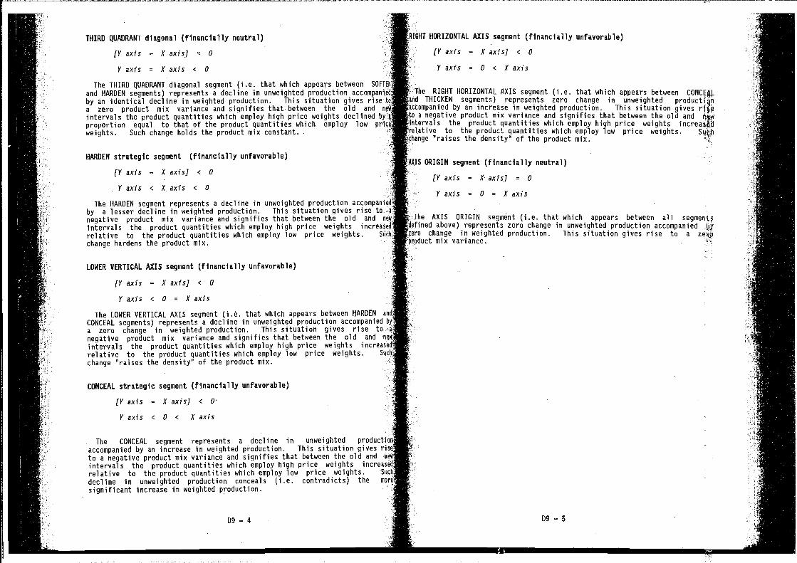
THIRD QUADRANT diagonal (financially neutral) RIGHT HORIZONTAL AXIS segment (financially unfavorable)
rv axis — X axis] = 0
V axis = X axis < 0
The THIRD QUADRANT diagonal segment (i.e. that which appears between SOFTEN
and HARDEN segments) represents a decline in unweighted production accompaniedby an identical decline in weighted production. This situation gives rise toa zero product mix variance and signifies that between the old and neW
intervals the product quantities which employ high price weights declined by aproportion equal to that of the product quantities which employ low priceweights. Such change holds the product mix constant.
HARDEN strategic segment (financially unfavorable)
(Y axis — X axis] < 0
V axis c X axis c 0
The HARDEN segment represents a decline in unweighted production accompanied'by a lesser decline in weighted production. This situation gives rise to a
negative product mix variance and signifies that between the old and new!
intervals the product quantities which employ high price weights increased!relative to the product quantities which employ low price weights. Such?
change hardens the product mix.
LOWER VERTICAL AXIS segment (financially unfavorable)
fY axis — X axis] c 0
V axis C 0 = A' axis
The LOWER VERTICAL AXIS segment (i.e. that which appears between HARDENa decline in unweighted production accompanied by
a zero change in weighted production. This situation gives rise to a
negative product mix variance and signifies that between the old and new
intervals the product quantities which employ high price weights increasedrelative to the product quantities which employ low price weights. Such
change "raises the density" of the product mix.
CONCEAL strategic segment (financially unfavorable)
(V axis — K axis] <
0 < Xaxis -
The CONCEAL segment represents a decline in unweighted productieiaccompanied by an increase in weighted This situation gives riseto a negative product mix variance and signifies that between the old and em
intervals the product quantities which employ high price weights increasedrelative to the product quantities which employ low price weights. Such
decline in unweighted production conceals (i.e. contradicts) the more
significant increase in weighted production. -
(V axis — K ax!s] < 0
V axis = 0 C K axis
T- The RIGHT HORIZONTAL AXIS segment (i.e. that which appears betweenand THICKEN segments) represents zero change in unweighted productiánaccompanied by an increase in weighted production. This situation givesto a negative product mix variance and signifies that between the old andintervals the product quantities which employ high price weights increasjdPelative to the product quantities which employ low price weights.
"raises the density" of the product mix.
AXIS ORIGIN segment (financially neutral)
[V axis — K-axis] = 0
V axis = 0 = K axis
'The AXIS ORIGIN segment (i.e. that which appears between alldefined above) represents zero change in unweighted production accompaniedtero change in weighted production. This situation gives rise to aproduct mix variance.
Log — 4 Dg — 5
a
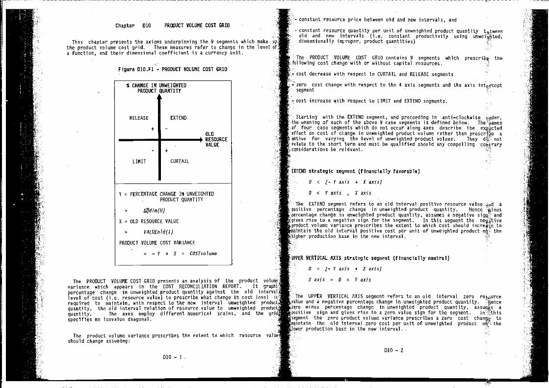
ri:
PRODUCT VOLUME COST GRID
This chapter presents the axioms underpinning the 9 segments which make up,
the product volume cost grid. These measures refer to change in the level ofa function, and their dimensional coefficient is a currency unit.
Figure D1O.FI - PRODUCT VOLUME COST GRID
—
The PRODUCT VOLUME COST GRID presents an analysis of the product volume
variance which appears in the COST RECONCILIATION REPORT. It graphspercentage change in unweighted product quantity against the old intervallevel of cost (i.e. resource value) to prescribe what change in cost levelrequired to maintain, with respect to the new interval unweighted productquantity, the old interval relation of resource value to unweighted productquantity. The axes employ different numerical scales, and the grid'specifies no isovalue diagonal.
The product volume variance prescribes the extent to which resource valueshould change assuming:
010—1-
— constant resource price between old and new intervals, and
— constant resource quantity per unit of unweighted product quantity Ltweenold and new intervals (i.e. constant productivity using
• dimensionally improper, product quantities)
The PROOUCT VOLUME COST GRID contains 9 segments which prescribe thefollowing cost change with or without capital resources.
— cost decrease with respect to CURTAIL and RELEASE segments
zero cost change with respect to the 4 axis segments and the axis interceptsegment
- cost increase with respect to LIMIT and EXTEND segments.
Starting with the EXTEND segment, and proceeding in anti—clockwise £*Vder,the eeaning of each of the above 9 case segments is defined below. The uaeesof four case segments which do not occur along axes describe the exppctedeffect on cost of change in unweighted product volume rather than amotive for varying the level of unweighted product volume. They notrelate to the short term and must be qualified should any compelling contraryconsiderations be relevant.
EXTEMD strategic segment (financially favorable)
0 < (—Vax/s * Xaxis]
0 < Vax/s , Xaxis
The EXTEND segment refers to an old interval positive resource value a
positive percentage change in unweighted product quantity. Hencepercentage change iii inweighted product quantity, assumes a negative and
-gives rise to a negative sign for the segment. In this segment the ne9jtiveproduct volume prescribes the extent to which cost should increfle to
the old interval positive cost per unit of unweighted product oh: thehigher production base in the new interval
The UPPER VERTICAL AXIS segment refers to an old interval zerovalue and a negative percentage change in unweighted product quantity. - Hence
minus percentage change in unweighted product quantity, assugks a
'positive sign and gives rise to a zero value sign for the segment. In-tthis'segment the zero product volume variance prescribes a zero cost tomaintain the old interval zero cost per unit of unweighted product oft thelower production base in the new interval . -
Chapter DiD
% CHANGE IN UNWEIGHTEDPRODUCT QUANTITY
RELEASE EXTEND
+OLDRESOURCE
VALUE- +
LIMIT CURTAIL
V = PERCENTAGE CHANGE IN UNWEIGHTEDPRODUCT QUANTITY
=
X = OLD RESOURCE VALUE
= VALUE0Pd(I)
PRODUCT VOLUME COST VARIANCE
= — V * K = COSTvoJumeUPPER VERTICAL AXIS strategic segment (financially neutral)
- 0 = (—Vax/s * Xaxis]
K axis = 0 < V axis
010 — 2
a
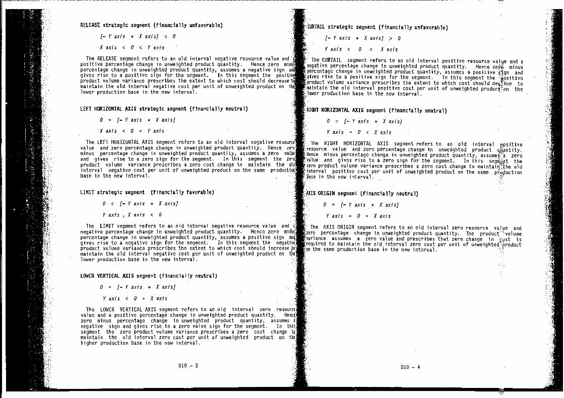
(— V axis * x axis] C 0
X axis < 0 < V axis
The RELEASE segment refers to an old interval negative resource value andpositive percentage change in unweighted product quantity. Hence zero minupercentage change in unweighted product quantity, assumes a negative sign aoi
gives rise to a positive sign for the segment. In this segment the positiviproduct volume variance prescribes the extent to which cost should decrease timaintain the old interval negative cost per unit of unweighted prodyct on thi
lower production base in the new interval.
LEFT HORIZONTAL AXIS strategic segment (financially neutral)
0 = (— V axis * X axis]
X axis < 0 = Y axis
The LEFT HORIZONTAL AXIS segment refers to an old interval negative resourcevalue and zero percentage change in unweighted product quantity. Hence zero
minus percentage change in unweighted product quantity, assumes a zero valUe
and gives rise to a zero sign for the segment. In this segment the zero
product volume variance prescribes a zero cost change to maintain the oldinterval negative cost per unit of unweighted product on the same productioubase in the new interval. -
LIMIT strategic segment (financially favorable)
0 < f—Yaxis * Xaxis]
V axis , X axis C 0
The LIMIT segment refers to an old interval negative resource value and a
negative percentage change in unweighted product quantity. Hence zero min'lis-
percentage change in unweighted product quantity, assumes a positive sign and
gives rise to a negative sign for the segment. In this segment the negativeproduct volume variance prescribes the extent to which cost should increase tomaintain the old interval negative cost per unit of unweighted product on th&lower production base in the new interval.
LOWER VERTICAL AXIS segment (financially neutral)
0 = 1— Y axis * X axis]
Y axis < 0 = X axis
The LOWER VERTICAL AXIS segment refers to an old interval zero resourcevalue and a positive percentage change in unweighted product quantity. Hence
zero minus percentage change in unweighted product quantity, assumes Inegative sign and gives rise to a zero value sign for the segment. In thissegment the zero product volume variance prescribes a zero cost change to
maintain the old interval zero cost per unit of unweighted product on the
higher production base in the new interval. -
(— V axis * X axis] > 0
Vaxis < 0 < Xaxis
The CURTAIL segment refers to an old interval positive resource value and a:negative percentage change in unweighted product quantity. Hence zeS minuspercentage change in unweighted product quantity, assumes a positive fign andgives rise to a positive sign for the segment. In this segment the jpsitiveproduct volume variance prescribes the extent to which cost should tomaintain the old interval positive cost per unit of unweighted product'on the
-lower production base in the new interval.
RIGHT HORIZONTAL AXIS segment (financially neutral)
0 = (— V axis * X axis]
V axis = 0 < X axis
The RIGHT HORIZONTAL AXIS segment refers to an old interval 1:psitiveresource value and zero percentage change in unweighted product
-Hence minus percentage change in unweighted product quantity, zerovalue and gives rise to a zero sign for the segment. In this thezero product volume variance prescribes a zero cost change to oldinterval positive cost per unit of unweighted product on the same pSoluctionbase in the new iiterval
AXIS ORIGIN segment (financially neutral)
= [— V axis * X axis]
V axis = 0 = X axis
The AXIS ORIGIN segment refers to an old interval zero resource vaiue andzero percentage change in unweighted product quantity. Thevariance assumes a zero value and prescribes that zero change in iust isrequired to maintain the old interval zero cost per unit of unweighted Øroducton the same production base in the new interval.
RELEASE strategic segment (financially unfavorable)-
CURTAIL strategic segment (financially unfavorable)
I
D1O— 3 010 — 4
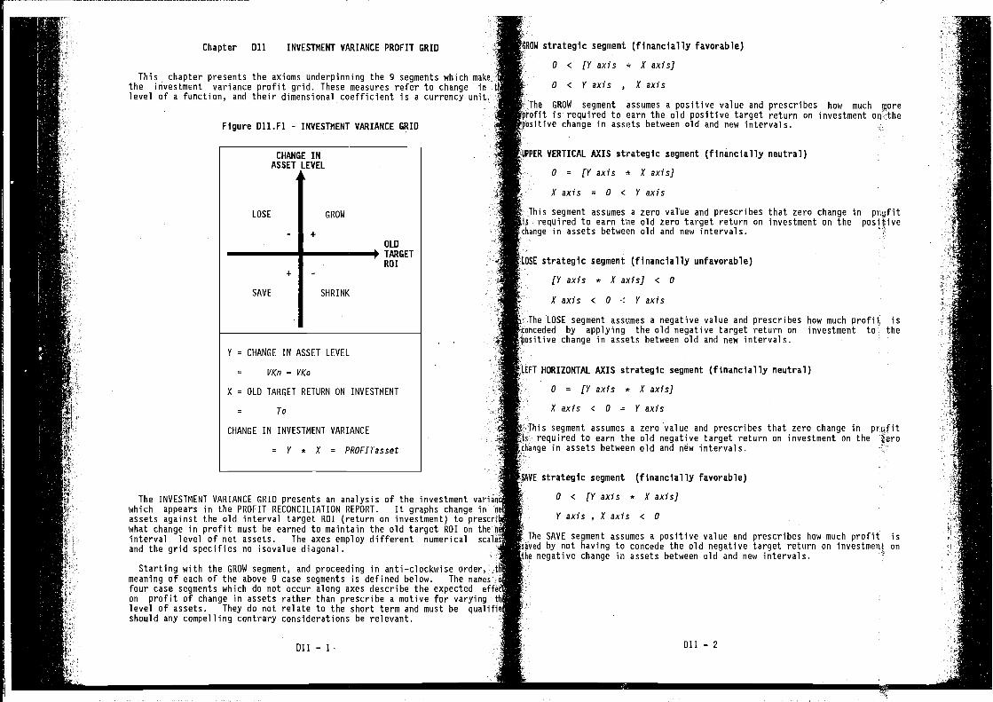
This chapter presents the axioms underpinning the 9 segments which ni-'-the investment variance profit grid. These measures refer to change inlevel of a function, and their dimensional coefficient is a currency
The INVESTMENT VARIANCE GRID presents an analysis of the investment variaiwhich appears in the PROFIT RECONCILIATION REPORT. It graphs change inassets against the old interval target ROI (return on investment) to prescwhat change in profit must be earned to maintain the old target ROI on theinterval level of net assets. The axes employ different numerical s
and the grid specifies no isovalue diagonal
Starting with the GROW segment, and proceeding in anti—clockwise order,meaning of each of the above 9 case segments is defined below. The namesfour case segments which do not occur along axes describe the expected e
on profit of change in assets rather than prescribe a motive for varyinglevel of assets. They do not relate to the short term and must be qualifshould any compelling contrary considerations be relevant.
Dli — 1
strategic segment (financially favorable)
0 < (V axis * K axis]
0 < Yaxis , Xaxis
GROW segment assumes a positive value and prescribes how much iaorejfit is required to earn the old positive target return on investment theositive change in assets between old and new intervals.
'PER VERTICAL AXIS strategic segment (financially neutral)
0 = TV axis * K axis]
K axis = 0 < Y axis
This segment assumes a zero value and prescribes that zero change inis required to earn old zero target return on investment on the positive
in assets between old and new intervals.
strategic segment (financially unfavorable)
(V axis * X axis] < 0
Kaxis < 0 Yaxis
The LOSE segment assumes a negative value and prescribes how much profit isby applying the old negative target return on investment to the
tive change in assets between old and new intervals.
HORIZONTAL AXIS strategic segment (financially neutral)
0 = (V axis * K axis]
K axis < 0 Y axis
This segment assumes a zero value and prescribes that zero change in profitrequired to earn the old negative target return on investment on the
ange in assets between old and new intervals.
strategic segment (financially favorable)
0 < [V axis * X axis]
V axis , K axis < 0
The SAVE segment assumes a positive value and prescribes how much profit is;aved by not having to concede the old negative target return on
in assets between old and new intervals.
Chapter Dli INVESTMENT VARIANCE PROFIT GRID
Figure D1l.Fl - INVESTMENT VARIANCE GRID
CHANGE INASSET LEVEL
LOSE GROW
+
+
OLD
TARGETROI
SAVE SHRINK
Y = CHANGE IN ASSET LEVEL
VKn — VK0
x= OLD TARGET RETURN ON INVESTMENT
To
CHANGE IN INVESTMENT VARIANCE
= Y*x = PROFiTasset
Dii — 2
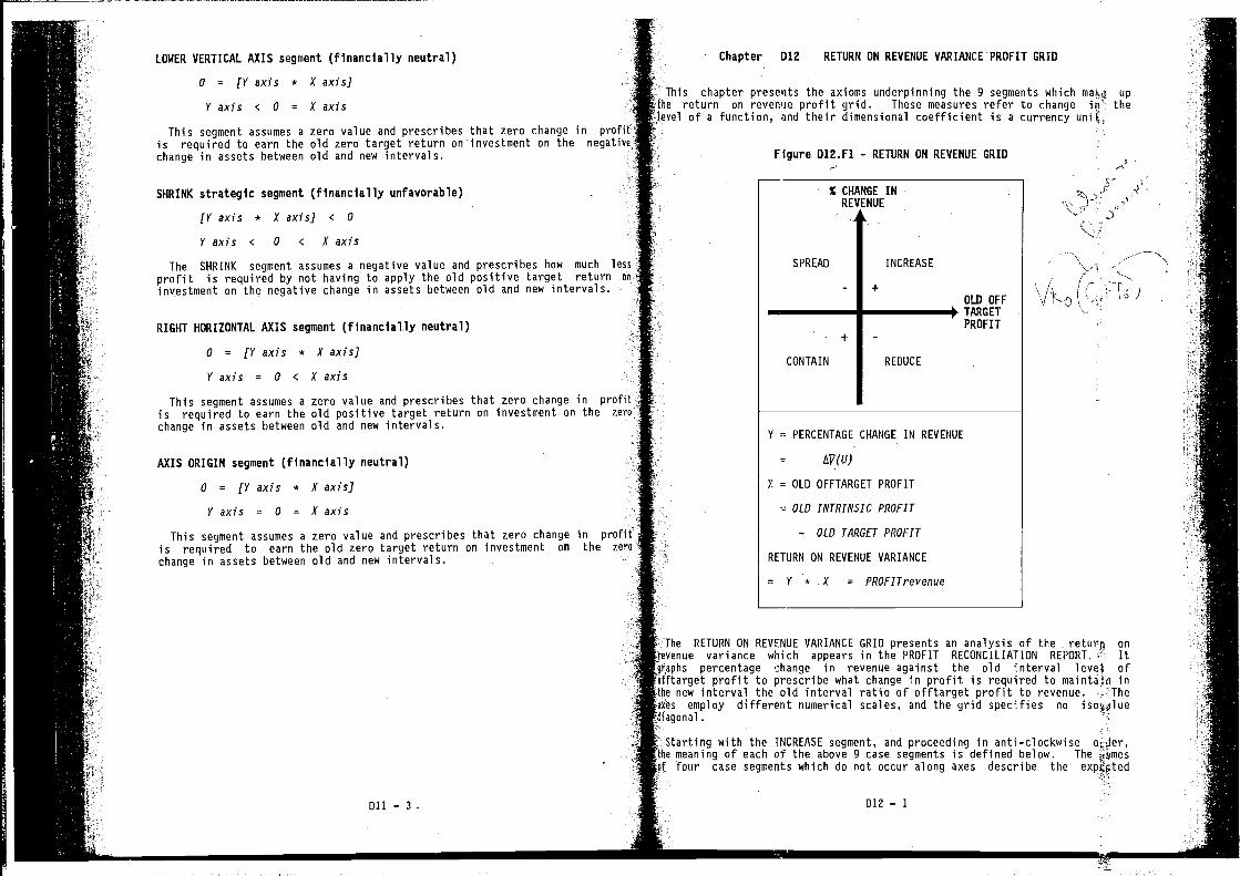
LOWER VERTICAL AXIS segment (financially neutral) Chapter 012 RETURN ON REVENUE VARIANCE PROFIT GRID
0 = (Y axis * X axis]This chapter presents the axioms underpinning the 9 segments which up
y axis < 0 = X axis return on revenue profit grid. These measures refer to change thelevel of a function, and their dimensional coefficient is a currency unit
This segment assumes a zero value and prescribes that zero change in profitis required to earn the old zero target return on investment on the negativechange in assets between old and new intervals. ' Figure D12.Fl - RETURN ON REVENUE GRID
SHRINK strategic segment (financially unfavorable) , % CHANGE IN '
REVENUE )-"(V axis * Xaxis] < 0 '4"
V axis c 0 c X axis
The SHRINK segment assumes a negative value and prescribes how much less SPREAD INCREASE N,
profit is required by not having to apply the old positive target return an - , ,r' '
investment on the negative change in assets between old and new intervals. +OLD OFF
RIGHT HORIZONTAL AXIS segment (financially neutral) - PROFIT-
0 = (V axis * X axis]CONTAIN REDUCE
Vaxis = 0 c Xaxis
This segment assumes a zero value and prescribes that zero change in profitis required to earn the old positive target return on investment on the zero
t change in assets between old and new intervals.V = PERCENTAGE CHANGE IN REVENUE
AXIS ORIGIN segment (financially neutral) = Loji(U)
= [V axis * X axis] ' 7 = OLD OFFTARGET PROFIT
V axis = 0 = X axis OLD INTRINSIC PROFIT
This segment assumes a zero value and prescribes that zero change in profit' — OLD TARGET PROFIT
is required to earn the old zero target return on investment on the zero
change in assets between old and new intervals. RETURN ON REVENUE VARIANCE
= V * X = PROFlTrevenue
The RETURN ON REVENUE VARIANCE GRID presents an analysis of the returg on- revenue variance which appears in the PROFIT RECONCILIATION REPORT. - It
graphs percentage change in revenue against the old interval level ofofftarget profit to prescribe what change in profit is required to mainta ii in
• the new interval the old interval ratio of offtarget profit to revenue. 'Theokes employ different numerical scales, and the grid specifies nodiagonal
Starting with the iNCREASE segment and proceeding in anti clockwisethe meaning of each of the above g case segments is defined below. The iiiomesof four case segments which do not occur along axes describe the
011 — 3 012 — 1
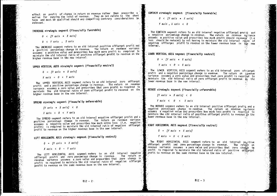
effect on profit of change in return on revenue rather than prescribe a
motive for varying the level of revenue. They do not relate to the short
term and must be qualified should any compelling contrary considerations be
relevant.
INCREASE strategic segment (financially favorable)
o < (V axis * X axis]
U < Y axis , X axis
The INCREASE segment refers to an old interval positive offtarget profit anda positive percentage change in revenue. The return on revenue variance
assumes a positive value and prescribes how much more profit is required to
maintain the old interval ratio of positive offtarget profit to revenue on thehigher revenue base in the new interval.
UPPER VERTICAL AXIS strategic segment (financially neutral)
o = (V axis * x axis]
X axis = U C Y axis
The UPPER VERTICAL AXIS segment refers to an old interval zero offtarget
profit and a positive percentage change in revenue. The return on revenue
variance assumes a zero value and prescribes that zero profit is required to
maintain the old interval ratio of zero offtarget profit to revenue on the
higher revenue base in the new interval
SPREAD strategic segment (financially unfavorable)
(Y axis * X axis] c U
X axis < U C V axis
The SPREAD segment refers to an old interval negative offtarget profit and apositive percentage change in revenue. The return on revenue variance
assumes a negative value and prescribes how much extra loss (i.e. negative
profit) is required to maintain the old interval ratio of negative offtargetprofit to revenue on the higher revenue base in the new interval.
LEFT HORIZONTAL AXIS strategic segment (financially neutral)
U = (V axis * X axis]
X axis < U = V axis
The LEFT HORIZONTAL AXIS segment refers to an old interval negative
offtarget profit and zero percentage change in revenue. The return on
revenue variance assumes a zero value and prescribes that zero change in
profit is required to maintain the old interval ratio of negative offtargetprofit to revenue on the same revenue base in the new interval
CONTAIN strategic segment (financially favorable)
U C (V axis * X axis]
V axis , X axis c U
The CONTAIN segment refers to an old interval negative offtarget profit anda negative percentage change in revenue. The return on revenue
a positive value and prescribes how much profit should (i.eloss should be reduced) by not having to maintain the old interval rfljo ofnegative offtarget profit to revenue on the lower revenue base in the newinterval
LOWER VERTICAL AXIS segment (financially neutral) -
U = (V axis * X axis]
V axis C U = X axis
The LOWER VERTICAL AXIS segment refers to an old interval zero oftt,argetprofit and a negative percentage change in revenue. The return onvariance assumes a zero value and prescribes that zero profit is tomaintain the old interval ratio of zero offtarget profit to revenue thelower revenue base in the new interval. -
REDUCE strategic segment (financially unfavorable)
(V axis- * X axis] < U
Yaxis < U < Xaxis
The REDUCE segment refers to an old interval positive offtarget profit and anegative percentage change in revenue. The return on revenue
a negative value and prescribes how much less profit is required tomaintain the old interval ratio of positive offtarget profit to revenue thelower revenue base in the new interval.
RIGHT HORIZONTAL AXIS segment (financially neutral)
U = (V axis * X axis]
V axis = U C X axis
The RIGHT HORIZONTAL AXIS segment refers to an old interval pqpitiveofftarget profit and zero percentage change in revenue. The onrevenue variance assumes a zero value and prescribes that zero in
- profit is required to maintain the old interval ratio of positiveprofit to revenue on the same revenue base in the new
012 —
I
012 — 3
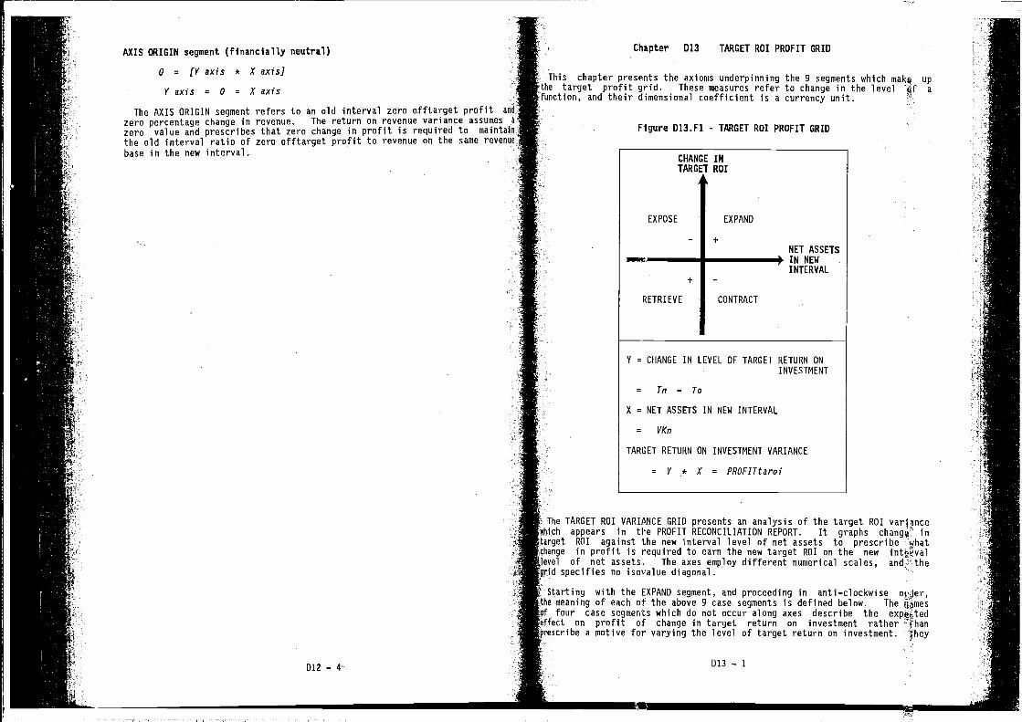
AXIS ORIGIN segment (financially neutral) Chapter D13 TARGET ROl PROFIT GRID
0 = (Y axis * K axis]This chapter presents the axioms underpinning the 9 segments which malce up
y axis = a = x axis the target profit grid. These measures refer to change in the level afunction, and their dimensional coefficient is a currency unit.
The AXIS ORIGIN segment refers to an old interval zero offtarget profit and
zero percentage change in revenue. The return on revenue variance assumeszero value and prescribes that zero change in profit is required to maintain Figure D13.FI - TARGET ROl PROFIT GRIDthe old interval ratio of zero offtarget profit to revenue on the same revenuebase in the new interval.
CHANGE INTARGET ROI
EXPOSE EXPAND
+NET ASSETSIN NEWINTERVAL
+ -
RETRIEVE CONTRACT
V = CHANGE IN LEVEL OF TARGET RETURN ONINVESTMENT
= Tn — To
X = NET ASSETS IN NEW INTERVAL
= VKn
TARGET RETURN ON INVESTMENT VARIANCE
= * K = PROFITtaroi
The TARGET ROl VARIANCE GRID presents an analysis of the target ROl variancewhich appears in the PROFIT RECONCILIATION REPORT. It graphs intarget ROI against the new interval level of net assets to prescribe whatchange in profit is required to earn the new target ROI on the newlevel of net assets. The axes employ different numerical scales, and theglid specifies no isovalue diagonal.
Starting with the EXPAND segment, and proceeding in anti—clockwise orjer,the meaning of each of the above 9 case segments is defined below. TheOf four case segments which do not occur along axes describe theeffect on profit of change in target return on investment ratherprescribe a motive for varying the level of target return on investment.
012—4 013—1
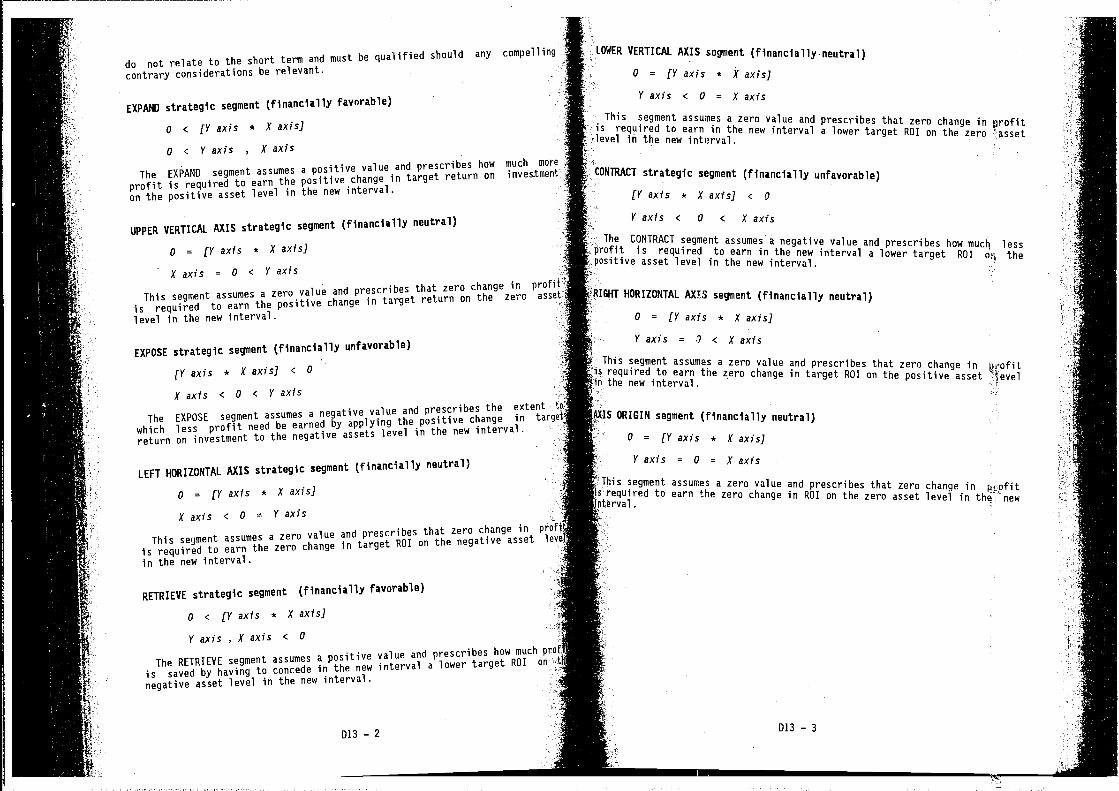
o = IY axis * X axis]
X axis = U < Y axis
This segment assumes a zero value and prescribes that zero change in profit
is required to earn the positive change in target return on the zero asset
level in the new interval.
EXPOSE strategic segment (financially unfavorable)
LY axis * X axis] < 0
X axis C 0 < Y axis
The EXPOSE segment assumes a negative value and prescribes the extent
which less profit need be earned by applying the positive change in targ
return on investment to the negative assets level in the new interval
LEFT HORIZONTAL AXIS strategic segment (financially neutral)
Q = fY axis * x axis]
Xaxis C 0 = Yaxis
This segment assumes a zero value and prescribes that zero change in preft!
is required to earn the zero change in target ROI on the negative asset
in the new interval
This segment assumes a zero value and prescribes that zero change in profitis required to earn in the new interval a lower target ROl on the zero'l in the new interval.
The CONTRACT segment assumes a negative value and prescribes how much lessprofit is required to earn in the new interval a lower target ROI thepositive asset level in the new interval
HORIZONTAL AXIS segment (financially neutral)
0 = [V axis * X axis]
Yaxis = U < Xaxis
This segment assumes a zero value and prescribes that zero change in Ps'ofitrequired to earn the zero change in target ROl on the positive asset levelthe new interval.
'5 ORIGIN segment (financially neutral)
0 = [V axis * Xaxis]
V axis = 0 = X axis
This segment assumes a zero value and prescribes that zero change in profitis required to earn the zero change in ROI on the zero asset level in the newiterval
do not relate to the short term and must be qualified should any compelling
contrary considerations be relevant.
EXPAND strategic segment (financially favorable)
o C (Y axis * X axis]
o < Y axis , X axis
The EXPANO segment assumes a positive value and prescribes how much mo
profit is required to earn the positive change in target return on inves.tment
on the positive asset level in the new interval.
UPPER VERTICAL AXIS strategic segment (financially neutral)
LOWER VERTICAL AXIS segment (financiallyneutral)
0 = [V axis * X axis]
V axis < 0 = X axis
CONTRACT strategic segment (financially unfavorable)
[V axis * X axis] < a
Vaxis < 0 c Xaxis
p
I
Lt
RETRIEVE strategic segment (financially favorable)
o c [V axis * X axis]
V axis , X axis < 0
The RETRIEVE segment assumes a positive value and prescribes how much prel
is saved by having to concede in the new interval a lower target ROI on I
negative asset level in the new interval.
013 — 2 013 — 3
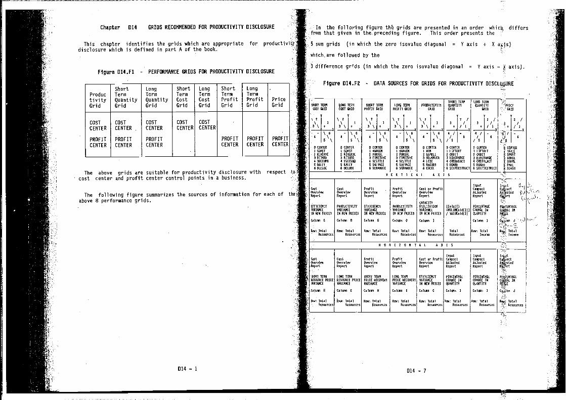
Chapter D14 GRIDS RECOMMENDED FOR PRODUCTIVITY DISCLOSURE
This chapter identifies the grids which are appropriate for productivitydisclosure which is defined in part A of the book.
Figure D14.Fl - PERFORMANCE GRIDS FOR PRODUCTIVITY DISCLOSURE
In the following figure grids are presented in an order which differsfrom that given in the preceding figure. This order presents the
5 sum grids (in which the zero isovalue diagonal = V axis + X axis)
whichare followed
3 difference grids
Figure D14.F2
ProductivityGrid
ShortTermQuantityGrid
LongTermQuantityGrid
ShortTermCostGrid
LongTermCostGrid
ShortTermProfitGrid
LongTermProfitGrid
.
PriceGrid
COSTCENTER
PROFITCENTER
COSTCENTER
PROFITCENTER
COST
CENTER
PROFITCENTER
COST
CENTER
COST
CENTER:
PROFITCENTER
PROFITCENTER
PROFITCENTER
by the
(in which the zero isovalue diagonal = V axis — X axis).
- DATA SOURCES FOR GRIDS FOR PRODUCTIVITY
SHtWT TERMQUARTIlEGRID
LENIG TERCI
COST GRID
0 CENTERI COAST2 RERER3E3 RETARE4 SRCCRNI
RALLY6 RELORE
SRONT TERM
PROFIT GRID
I CENTERI AWAKEN2 PARYYE3 FINETRRE4 OCOTTLES SALRACE6 SCRAWRLE
TERN
PROFIT GRID±0 CENTER1 AWAKEN2 PARYAE3 FINETYREV OCATTLES SALVAGE6 SCRAMILE
PRWACTIAITTORIR
CENTER
1 62W2 ORWRLE3 SRUANAER4 LOSE5 ARTOAN6 EACEL
IRENT TERNCOOT GRID
CENTER
I COAST2 RERERTE3 RETARD4 RACER MR
I RALLY6 DELUDE
tootReerelowReport
OFFICIENCTAMIANCEIN NEW PRICES
Column 0
Row: TotalReooorteo
LERO TERNRAW WIITT
GRID
S CENTER1 LIFIOFF2 ARRIT3 OIRCVAROE4 OVERREACT
WOARD
6 SELFSESSYACT
O CENTER2 LIFTOFFO ERIIT3 RISCRARGE4 OVERREACT5 WAAREN SELFEESIRACT
RERTICAL AS S
CootOverviewReport
PRARACTIRSTOWAR lAN C E
IN NEW PRICES
Colomv E
Row: TotalReooorceo
PRICE- GRID
CEWTER
4 TRAILo SPORT4 RUSE5 SVAAE
FARE
* SLASA
LLj'2PhSOENTAGE
IN
3
ENOvol Total
Income
ProfitOverviewReport
EFFICIENCYTARIANCEIN NEW PRICES
Column 0
Roe: TotalReooorceo
ProfitOverviewReport
FREN2ACTIRITTRARIANCEIN NEW PRICER
Coloov 0
Roe: TotalReooorceo
The above grids are suitable for productivity disclosure with respect to
cost center and profit center control points in a business.
The following figure summarizes the sources of information for each ofabove 8 performance grids.
D14 — 1
Coot or ProFitOoero lowReport
CVPVCITYUTILIZATIONRARUANCE
IN NEW PRICER
Colomv I
Woe: TotalReooorceo
IvpotCoopoctAdjoo tedReport
FERCLNYAGE
CVAWGE INOAAWTITT
Colown I
Row: TotalIncome
(to ld( I(+YALARL01d(IlI/ WALOEo14(I)
TotalReooorcoo
RU IZRNRAL AOIR
H
tootOverviewNeport
MART TERNREIRIRCE PRICENON lANCE
Column W
CootOverviewReport
LONG TERNRESMJRCE PRICERARIARCE
Column E
ProFitOverviewReport
SWCNT TERNPRICE RECORERYRN1IAWCE
Colomv W
Row: TotalRoooorceo
Coot or ProFItOverviewReport
EFFICIENCYWAR lANCE
IN NtN PRICES
Colown 0
ProfitOverviewReport
LONG TERNPAICE RCCSVEATVARIANCE
Colomo E
Row: TotalReoourcoo
lopotCompactAdjuotedReport
PERCENTAGE
CRANGE INOUANTITT
Coloioo I
Now: Total Row: TotalReooorcoo Roooorcno
InputCompactAdjuotedReport
PERCENTAGE
CWANGE IN
IRANYITA
Colomo I
tC4000E IN
Roe: TotalR000urceo
Row: Total Wow: Total Wow: TotalReooorceo Roooorcoo Roooorcno
k
D14 — 7
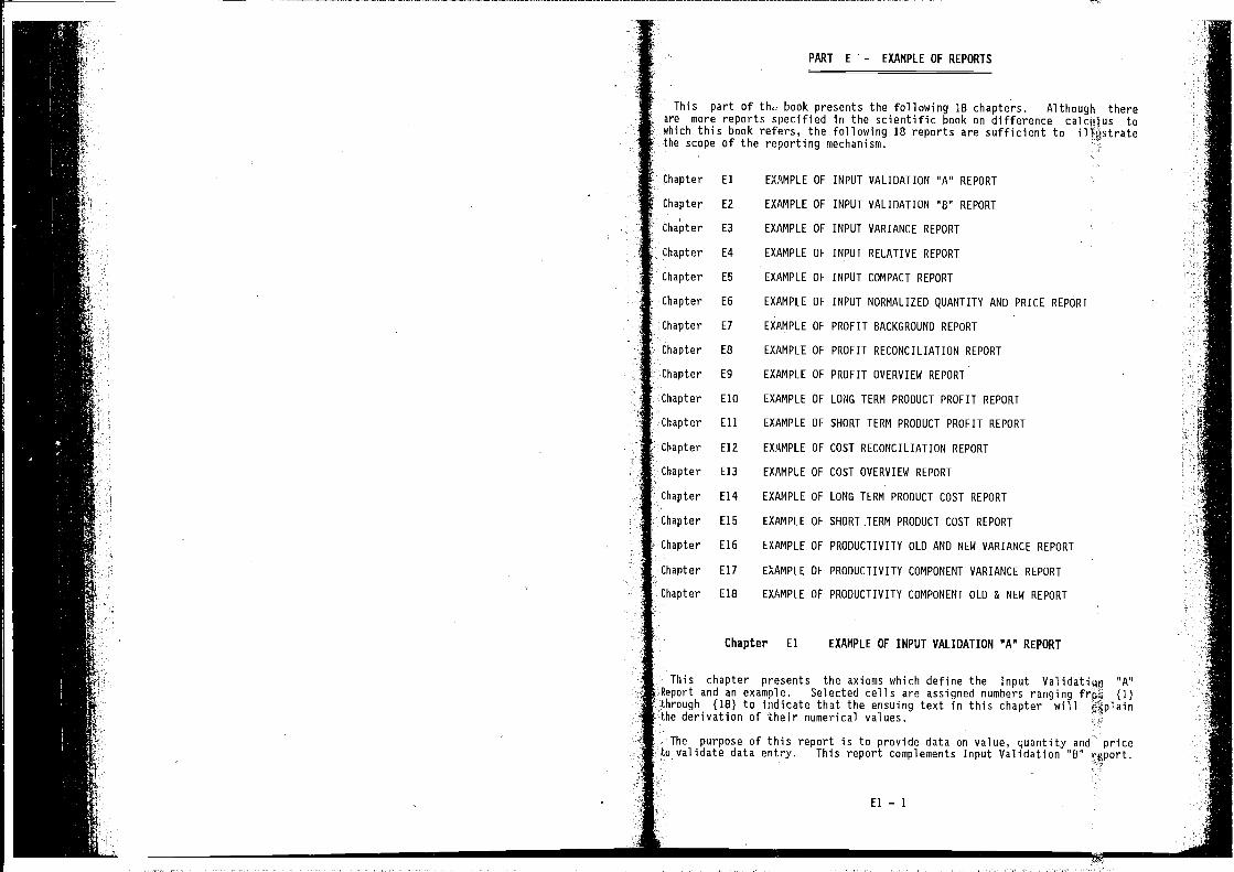
PART E - EXAMPLE OF REPORTS
This part of book presents the following 18 chapters. Although thereare more reports specified in the scientific book on difference towhich this book refers, the following 18 reports are sufficient to iltustratethe scope of the reporting mechanism.
Chapter El EXAMPLE OF INPUT VALIDATION 'A" REPORT
Chapter E2 EXAMPLE OF INPUT VALIDATION "B" REPORT
E3 EXAMPLE OF INPUT VARIANCE REPORT
Chapter E4 EXAMPLE OF INPUT RELATIVE REPORT
Chapter E5 EXAMPLE OF INPUT COMPACT REPORT
Chapter E6 EXAMPLE OF INPUT NORMALIZED QUANTITY AND PRICE REPORT
Chapter E7 EXAMPLE OF PROFIT BACKGROUND REPORT
Chapter EB EXAMPLE OF PROFIT RECONCILIATION REPORT
Chapter E9 EXAMPLE OF PROFIT OVERVIEW REPORT
Chapter ElO EXAMPLE OF LONG TERM PRODUCT PROFIT REPORT
Chapter EI1 EXAMPLE OF SHORT TERM PRODUCT PROFIT REPORT IChapter E12 EXAMPLE OF COST RECONCILIATION REPORT
Chapter EI3 EXAMPLE OF COST OVERVIEW REPORT
Chapter E14 EXAMPLE OF LONG TERM PRODUCT COST REPORT
Chapter E15 EXAMPLE OF SHORT TERM PRODUCT COST REPORT
Chapter E16 EXAMPLE OF PRODUCTIVITY OLD AND NEW VARIANCE REPORT
Chapter E17 EXAMPLE OF PRODUCTIVITY COMPONENT VARIANCE REPORT
Chapter E1B EXAMPLE oF PRODUCTIVITY COMPONENT OLD & NEW REPORT
Chapter El EXAMPLE OF INPUT VALIDATION "A" REPORT
This chapter presents the axioms which define the Input Validatiup "A"Report and an example. Selected cells are assigned numbers ranging frpe (I)through (18) to indicate that the ensuing text in this chapter willthe derivation of their numerical values. 1
The purpose of this report is to provide data on value, quantity and priceto validate data entry. This report complements Input Validation "B" report.
El — 1
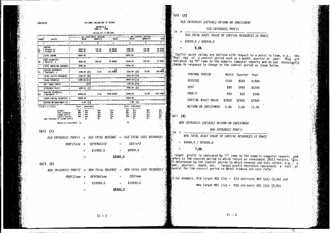
E1—2 E1—3
1989/09/Il PPM INPUT VALIDOTIFAI 0" REP80T
BUSINESS A1981 vs. 1989
Values are in DOLLARS
OLD (REFEDENCE) INTERVAL NEW (DEVIEW) INTEUVAL
INDEX ENTITY VALUE QUANTITY PRICE VALUE QUANTITY PRICI
I IU U C I E FL
INCOME:
UI Prsduct aI 6000.01 150.00 40.00000 1901.00 000.00 44.10000
02 Prsduct a2 4000.00 84.00 11.00001 9100.00 — — 140.00 60.00004
I(IXTAL INCOME 10000.00 18001.00
COST REX OIJRCES:
Ni Naterial a 8000.00 400.00 20.00000 12540.00
= 5,0%
570.00 22.00000
ITOTAL OPERATING EXPENSES 8000.00 12540.00
CAPITAL RESU1RCES:Ti Equipment a
[7) (8
1100.00 (5) 8.00 250.00100 3500.00 (6) 10.00 350.0000
TOTAL CAPITAL REOOJRCES 1000.00 (9) 3500.00 [II)
TOTAL RESO'JRCES 10000.00 (II) 16040.00 (12) I
TARSET PROFIT (13] 1960.00 (14)I
INTRINSIC PROFIT 2000.00 (1) . - 5460.00 [2) -
CAPITAL RESWRCES:KS Equipment a 40000.00 8.00 5001.00001 70000.00 10.00 7000.00014
ITOTAL CAPITAL RESWRCES 40000.00 71005.A0 I—
IRE1SRN 001 INOESTNENT (0) 5.00 [3) 7.80 (4) I
PUN CT I ON S Tstal Individual Tstal Individual
cest resnurce
prndsctcsst ressurcetarget prsfltcapital assetssr Sarget preP it
VOn
ANn
ATsADs
VusOne
Yts• VAn
Ye
RueRevQtaRAn
Ru
PusPenPEnPksPs
NonANn
ATnVOn
• NunYenVtnVAnAn
QusQnnQtnRAnRn
Pun
Pen
PinPA'Pn
,
'
Return On Onnesteent Cs
Cell (1)
Ce
CAPITAL ASSET VALUE
RETURN ON INVESTMENT
Cell (3)
OLD INTRINSIC (ACTUAL) RETURN ON INVESTNENT
OLD INTRINSIC PROFITCo
OLD TOTAL ASSET VALUE OF CAPITAL RESOURCES (K ROWS)
= $2000,O / $40000,0
Capital asset values are defined with respect to a point in time, e.g., thefinal day of a control period such as a month, quarter or year. They areiRdicated by sKe rows in the numeric computer reports and do not necessarilychange in response to change in the control period as shown below.
CONTROL PERIOO Month Quarter Year
REVEIIUE $100 $500 $1500
COST $80 $450 $1200
PROFIT $20 $50 $300
$2500 $2500 $2500
-0,8% 2,0% 12,0%
Cell (4)
,-Cn
= 7,8%
Target profit is indicated by rows in the numeric computer reportsrefers to the control period to which return on investment (ROl) relates. ThisIs determined by the control period to which revenue and cost relate, e.g.; ayear, quarter, month, etc. Target profit therefore represents a cost: ofCapital for the control period to which revenue and cost refer.
In our example, Old Target ROI (To) = Old Intrinsic ROl (Co) (5,0%) and
New Target ROl (Tn) = Old Intrinsic ROI (Ce) (5,0%)
Cell (2)
NEW INTRINSIC (ACTUAL) RETURN ON INVESTNENT
NEW INTRINSIC PROFIT
OLD INTRINSIC PROFIT e OLD TOTAL REVENUE — OLD TOTAL COST RESOURCES
PROFITo1d REVENUEo!d — COSToJd
= $I0000,O — $8000,O
$2000,0 :.
NEW INTRINSIC PROFIT NEW TOTAL REVENUE — NEW TOTAL COST RESOURCES
PROFITnoW a REVENUEnoW — COSTnew
= $18000,0 — $1254O,O
NEW TOTAL
= $546O,O /
ASSET VALUE OF CAPITAL RESOURCES (K ROWS)
$ 70000,0
$5460,0
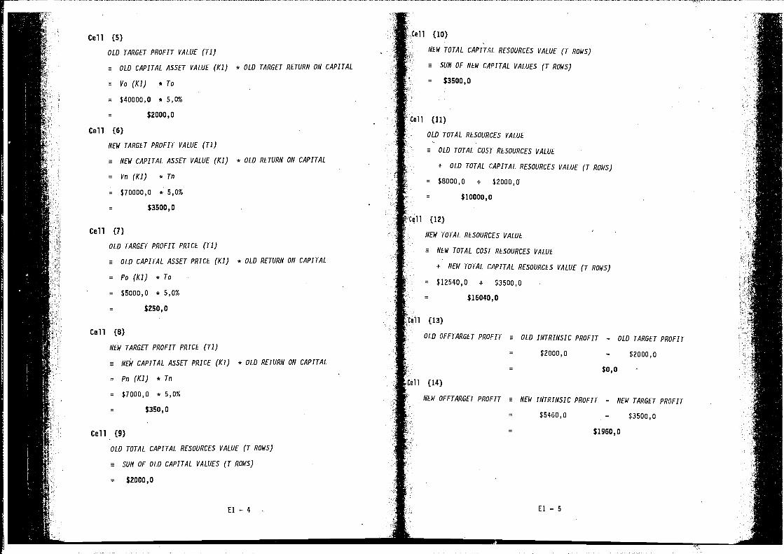
Cell (5)
OLD TARGET PROFIT VALUE (Ti)
E OLD CAPITAL ASSET VALUE (Ki) * OLD TARGET RETURN ON CAPITAL
= Vo(Ki) *To
= $40000,0 * 5,0%
= $2000,0
Cell (6)
NEW TARGET PROFIT VALUE (Ti)
E NEW CAPITAL ASSET VALUE (Ki) * OLD RETURN ON CAPITAL
= Vn(Ki) *Tn
$70000,0 * 5,0%
$3500,0
Cell (7)
OLD TARGET PROFIT PRICE (Ti)
OLD CAPITAL ASSET PRICE (Ki) * OLD RETURN ON CAPITAL
= Po (Ki) * To
= $5000,0 * 5,0%
= $250,0
Cell (8)
NEW TARGET PROFIT PRICE (Ti)
NEW CAPITAL ASSET PRICE (Ki) * OLD RETURN ON CAPITAL
= Pn (Ki) * Tn
= $7000,0 * 5,0%
= $350,0
Cell (9)
OLD TOTAL CAPITAL RESOURCES VALUE (T ROWS)
SUM OF OLD CAPITAL VALUES (T ROWS)
= $2000,0
Cell (10)
NEW TOTAL CAPITAL RESOURCES VALUE (T ROWS)
E SUN OF NEW CA°ITAL VALUES (T ROWS)
= $3500,0
Cell (11)
OLD TOTAL RESOURCES VALUE
E OLD TOTAL COST RESOURCES VALUE
+ OLD TOTAL CAPITAL RESOURCES VALUE (T ROWS)
= $8000,0 + $2000,0
= $10000,0
:-Cell (12)
NEW TOTAL RESOURCES VALUE
E NEW TOTAL COST RESOURCES VALUE
£
÷ NEW TOTAL CAPITAL RESOURCES VALUE (T ROWS)
= $12540,0 + $3500,0
Cell (14)
NEW OFFTARGET PROFIT NEW INTRINSIC PROFIT - NEW TARGET PROFIT
= $5460,0 — $3500,0
$16040, 0
Cell (13)
OLD OFFTARGET PROFIT OLD INTRINSIC PROFIT
= $2000,0
— OLD TARGET PROFIT
— $2000,0
$0, 0
E1—4
L
$ 1960,0
El — 5
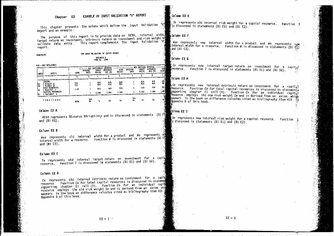
N/H NOT
INTERNAL KEN (REVIEW) INTERVAL
INDEA ENDITT
OLD (REFERENCE)INTERVAL TARGET INTRINSIC RISK INTERVAL TAROET INTRINSIC
RENA DAYS ROI)G) RRI (8) WEIGHT DAYS RGI)S) Vol )S)
F S H
I IA D C D E
INCENSE:
UI Product aI N/AI N/A N/A
N/A I N/A N/A N/A N/A N/A
1 N/AN/A
a
1 1.880 1.800
Column E2 A
REVuI represents REsource VAriabilitY and is discussed in statements (B] F
and (81 F2).
Column E2 B
Woo represents old interval width for a product and Wa represents
interval width for a resource. Function W is discussed in statements (81
and (81 C2).
Column E2 C
To represents old interval target return on investment for a cai
resource. Function T is discussed in statements (81 01) and (81 02).
Column E2 D
Co represents old interval intrinsic return on investment for a cap
resource. Function Co for total capital resources is discussed in staten!
supporting chapter El cell (3), Function Co for an individual ca'
resource employs the old risk weight So and is derived from an ark:appears in the book on difference calculus cited as bibliography itemAppendix B of this book.
Column E2 E
So represents old interval risk weight for a capital resource. Function Sdiscussed in statements (81 El) and (81 E2).
Wun represents new interval width for a product and Wn represents'erval width for a rosource. Function W is discussed in statements (81 tj)d (81 C2). -'
Tn represents new interval target return on investment for aesource. Function T is discussed in statements (81 Dl) and (81 02).
represents new interval intrinsic return on investment for a1source. Function Cn for total capital resources is discussed inipporting chapter El cell (4). Function Cn for an individual capitalDseurce employs the new risk weight Sn and is derived from an axiomopears in the book on difference calculus cited as bibliography item A15sendix B of this book.
represents new interval risk weight for a capital resource. Function £ Hdiscussed in statements (81 El) and (81 E2)
E2 I
Chapter E2 EXAMPLE OF INPUT VALIDATION "B" REPORT
This chapter presents the axioms which define the Input Validation
Report and an example.
The purpose of this report is to provide data on REVA, interval wT
target return on investment, intrinsic return on and risk weight
validate data entry. This report complements the Input Validation 'H
report.
IDea/ON/UIFPN INPUT RALIDNTIENS 'I' ENTITT REP88T
DUllNESS A1888 vs. 1888
nE2F
Column E2 C
FDNCTIDND Nue
REAA No To
E2 H
Ave
Cu Iv No Dv Ce
E2 — 1 - E2 — 2
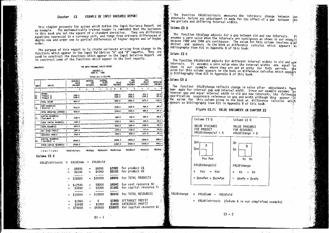
Chapter E3 EXAMPLE OF INPUT VARIANCE REPORT
This chapter presents the axioms which define the Input Variance Report and
an example. The mathematically trained reader is reminded that the variancesin this book are not the square of a standard deviation. They are differenceequations expressed in a currency unit, and range from ordinary differences efdegree one and order one to partial differences of higher degree and of higherorder.
The purpose of this report is to create variances arising from change in thefunctions which appear in the Input Validation "A" and "B" reports. They -areused to construct the functions which appear in the Input Relative Report and
to construct some of the functions which appear in the Cost reports.
PPM INPUT RAeIANCE ENTITY REPAST
BOSINESS Aegeevo. IRAN
Values are In 00I.LPAS
INleiNsic IVTEVVAL INTERVAL PURE PURE
VALUE GAP ROOm VALUE RALURE PRICE
INRES ENTITY VARIANCE VARIANCE VARIANCE VARIANCE VARIANCE VARIANCE
E + P + II I j A B +' C +0
INCASE:US Product alAl Product aO
—
2100.0 2900.0 0000.0 675.0 211.0
5100.0 5100.0 3000.0 1200.0 000.0
1121.;TOTAL INCeNE ROOtS R000.0 5000.0 ieis.e
CAST RESOURCES:
NI Material a - 4540.0 - - 4540.0 — 3400:0 800.0 - 340.0
3410.0 RVV.U 340.1I
ITOTAL OPERATING EAPENSES NR4V.U 454V.R
=CAPITAL RESOURCES:
Ti EVuIPISeOL a 1505.5 1500.0 500.0 eoo.e 200.0
TOTAL CAPITAL RESOURCES 1500.0 1500.0 500.0 800.0 200.0
=ITOTAL RESOURCES 4540.5 6040.0 3900.2 1600.0 140.0
CAPITAL RESOURCES:KO Equipment a 30000.0 30000.0 10000.0 16000.0 4002.0
IITOTAL CAPITRL RESOURCES 30005.5 30000.0 IR005.V 16000.0 4000.0
=
=
$8900$9100
—
— $4000 $5100 for product U2
= $18000 — $10000 $8000 for TOTAL PROOUCTS
=
=
=
$12540$3500
$16040
—
—
—
$8000$2000
$10000
$4540 for cost resource NI$1500 for capital resource TI
$6040 for TOTAL RESOURCES
=
=
=
$1960$5460
$70000
—
—
—
0
$2000$40000
$1960 OFFTARGET PROFIT
$3460 INTRINSIC PROFIT$30000 for capital resource Ki
'
The function VALLJEintrinsic measures the intrinsic change between twointervals before any adjustment is made for the effect of a gap between thetwo periods and differing interval widths.
Column E3 B
The function V.4LUEgap adjusts for a gap between old and new intervals. Itassumes a zero value when the intervals are contiguous as shown in our examplebecause 1989 and 1988 are contiguous. The axiom for this column involvesdivisor and appears in the book on difference calculus which asbibliography' item AI5 in Appendix 8 of this book.
Column E3 C
The function VALUEWIdtA adjusts for different interval widths in old and I0ewintervals. It assumes a zero value when the interval widths are equal tasshown in our example where they are set at unity for both periods.axiom for this column appears in the book on difference calculus which appe4rsas bibliography item AlS in Appendix B of this book.
Column E3 0
The function VALUEchange reflects change in value after adjustmentsbeen made for interval gap and interval width. Since our example assumes jointerval gap and equal interval width in old and new intervals, thespecification suppresses reference to gap and width although they appear linthe axiom for this column given in the book on difference calculus whijjhappears as bibliography item A15 in Appendix B of this book.
Figure E3.Fl VALUE VARIANCES IN CHAPTER E3
Column F3 0, Column E3 0
VALUE VALUE VARIANCEFOR PRODUCT FOR RESOURCEVALUEchange(u) = A VALUEchange = B
REPRICING
VARIANCE
TARGET PROFIT
IINTVINSSC PROFIT
1960.0
3460.0
1960.0 1000.0
3460.0
275.0
1600.0
501.0
1075.0 785.0
P U N C 1 1 5 N S RALAEIntrInuic AALSEqap AALAEuIdLh RALUCchange VOLUNEo1d
Column E3 A
VALUEintrinsic VALUEnew — VALUEo7d
PRICEuId PRICErep
Puo Pun
VALUEchange (a)
a Van — Vito
= Qun*Pun — Quo*Pao
0
Po Pn
VALUEchange
a Vn — Vo
= Qn*Pn — Qo*Po
A
VALUEchange a V/1LUEITeW — VALUEo!d
= VALUEintrinsjc (Column A in our simplified example)
E3 — 2
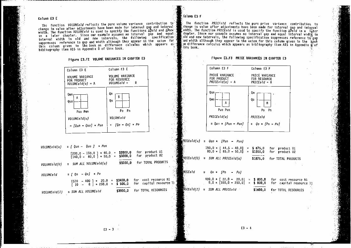
Column E3 E
The function VOLUMEoId reflects the pure volume variance contribution to
change in value after adjustments have been made for interval gap and intervalwidth. The function VOLUMEo1d is used to specify the functions and
in a later chapter. Since our example assumes no interval gap and equal
interval width in old and new intervals, the following specification
suppresses reference to gap and width although they appear in the axiom for
this column given in the book on difference calculus which appears as
bibliography item A15 in Appendix B of this book.
Figure E3.F2 VOLUME VARIANCES IN CHAPTER E3
Column E3 F
The function PRICFo!d reflects the pure price variance tochange in value after adjustments have been made for interval and
i. The function PRICEoId is used to specify the function in a later- "r. Since our example assumes no interval gap and equal interval width inand new intervals, the following specification suppresses referencewidth although they appear in the axiom for this column given in the
on difference calculus which appears as bibliography item A15 in Appendix ofthis book.
Figure E3.F3 PRICE VARIANCES IN CHAPTER E3
PRICE VARIANCE PRICE VARIANCEFOR PRODUCT FOR RESOURCEPRICEo7d(u) = A PRICE0Id = B
Qun -
Puo Pun
PRICEo !d(u)
a * [Pun — Puo]
Qn
Qo * (Pn — P0]
$2000,O$3000,O
$5000,O
for cost resource Nifor capital resource Ti
150,0 * [ 44,5 — 40,0] =
80,0 * [ 65,0 — 50,0] =for product Uifor product U2
for TOTAL PRODUCTS
for cost resource Nifor capital resource
for TOTAL RESOURCES
VOLUMEoJd(U) a ( Qun — Quo J * Puo
[200,0 — 150,0 1 * 40,0 =
[140,0 — 80,0 ] * 50,0 =
VOLUME01d(U) a SUM ALL VOLUMEoJd(u)
VOLUMEOId a ( Qn — Qo] * P0
for product Uifor product U2
for TOTAL PRODUCTS
Eold(u) a Quo * [Pun — Puo]
[570 — 400 1* 20,0 = $3400,O
10 — 8 1* 250,0 = $ 500,0
VOLUMEo1d(I) a SUM ALL VOLUMEoId $3900,O for TOTAL RESOURCES
$ 675,0$ 1200,0
a SUM ALL PRICEo7d(u) $1875,O
a Qo * (Pn — Po]
400,0 * [ 22,0 — 20,0] = $ 800,08,0 * [350,0 — 250,0] = $ 800,0
CEo7d(I) a SUM ALL PRICEo1d $1600,0
E3 — 4E3—3 -
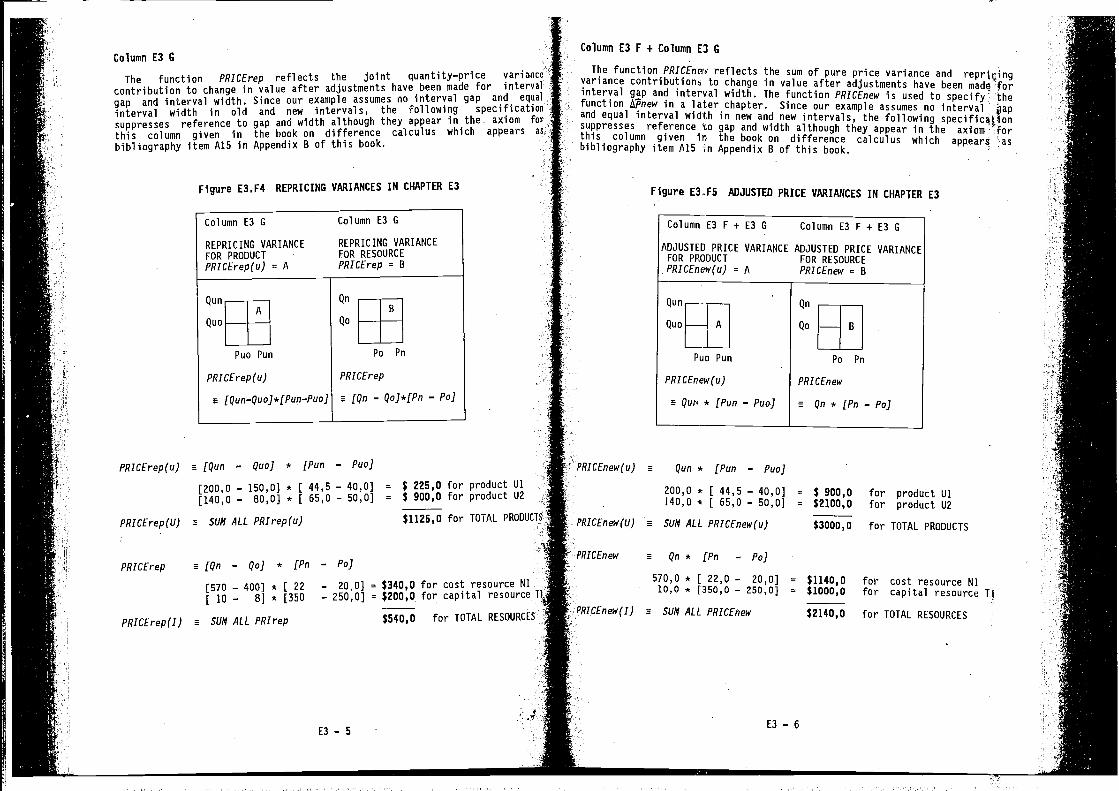
Column E3 C
The function PRICErep reflects the joint quantity—price variancecontribution to change in value after adjustments have been made for intervalgap and interval width. Since our example assumes no interval gap and e#:1
interval width in old and new intervals, the following specificationsuppresses reference to gap and width although they appear in the- axiom for
this column given in the book on difference calculus which appears as
bibliography item A15 in Appendix B of this book.
Figure E3.F4 REPRICING VARIANCES IN CHAPTER E3
Column E3 G Column E3 G
REPRICING VARIANCE REPRICING VARIANCEFOR PRODUCT FOR RESOURCE
PRICErep(u) = A PRICErep = B
Puo Pun
PRICErep (u)
e fQun—QuoJ*(PUP—PLlO]
Po Pn
PRICErep
a (Qn — QoJ*[Pn — Pa]
Column E3 F + Column U C
The function PRICEncr.v reflects the sum of pure price variance andvariance contributions to change in value after adjustments have beeninterval gap and interval width. The function PRICEnew is used to specify thefunction A7new in a later chapter. Since our example assumes no interval flpand equal interval width in new and new intervals, the following specificfl'lonsuppresses reference to gap and width although they appear in the axiomthis column given in the book on difference calculus which appears -asbibliography item AIS Appendix B of this book.
Figure E3.F5 ADJUSTED PRICE VARIANCES IN CHAPTER E3
Column E3 F + [3 G Column E3 F + E3 G
ADJUSTED PRICE VARIANCE ADJUSTED PRICE VARIANCEFOR PRODUCT FOR RESOURCEPRICEnew(e,) A PRICEnew = B
•
Puo Pun
PRICEnew(u)
aQur*[Pun—Pua]
Po Pn
PRICEnew
a
PRICErep(u) a (Qun — Quo] * (Pun — PuoJ
[200,0 — 150,0] * [44,5 — 40,0] = $ 225,0 for product UI[140,0 — 80,0] * [65,0 — 50,0] = $ 900,0 for product U2
PRICErep(U) a SUM ALL PRIrep(u) $1125,D for TOTAL PRODUCTS
PRICErep a (Qn — Qo] * (Pn — Po]
[570 — 400] * [ 22
[10— 8]*[350
PRICErep(I) a SUM ALL PRirep
570,0 * [ 22,0 — 20,0] = $1140,010,0 * [350,0 — 250,0] = $I000,o
for cost resource Nifor capital resource
PRICEnew(u) a Qun * [Pun — Puo]
200,0 * [ 44,5 — 40,0] = $ 900,0140,0 * [ 65,0 — 50,0] = $2100,0
for product UIfor product U2
PRICEnew(1J) a SUM ALL PRICEnew(u) $3000,D for TOTAL PRODUCTS
PRICEnew a Qn * (Pn — Po]
— 20,0] = $340,0 for cost resource Ni— 250,0] = $200,0 for capital resource
$540,0 for TOTAL RESOURCES
E3 — 5
PRICEnew(I) a SUM ALL PRICEnew $2i40,0 for TOTAL RESOURCES
E3 — 6
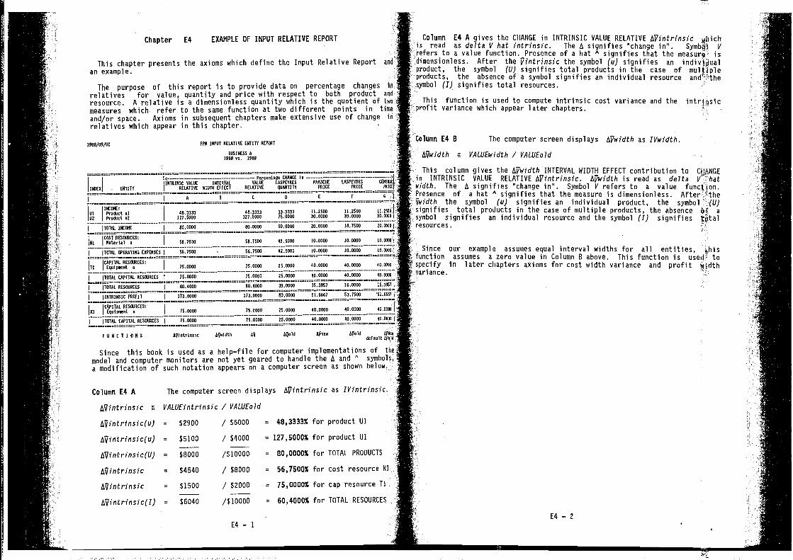
Chapter E4 EXAMPLE OF INPUT RELATIVE REPORT
This chapter presents the axioms which define the Input Relative Report and
an example.
The purpose of this report is to provide data on percentage changes in
relatives for value, quantity and price with respect to both product and
resource. A relative is a dimensionless quantity which is the quotient of twomeasures which refer to the same function at two different points in time
and/or space. Axioms in subsequent chapters make extensive use of change in
relatives which appear in this chapter.
1988/09/01 FPN INPUT RELATIVE ENTITY REPcNT
BUSINESS A1988 vs. 1989
Percentage CHANGE inINTERVAL VALUE LASPEYRES
WIDTH EFFECT RELATIVE qUANTITY
IA B C 0 C F 0
INCOME:
01 Product al02 Product a2
48.3333 48.3333 33.3333 11.2500 11.1000 11.2001
127.8000 127.0002 70.0000 30.0000 30.0000 30.0022
ITOTAL INCOME 00.0000 80.0000 SO.0000 20.0000 18.7000 20.0022
COST RESOURCES:
NI Material a 50.7500 — —— 56.7000 — 42.5000 10.0000 20.0000 20.0000
IIIOTAL OPERATINI EUPERSES 50.7500 - 56.7500 02.5000 10.0000 60.0000 10.0001
CAPITAL RESOURCES:TI Equipment a 75.0000 75.0000 21.0000 40.0000 00.0000 40.0000
ITOTRI CAPITAL RESOURCEST
75.0000 75.0000 25.0000 40.0000 00.0000 40.0002
39.0000 15.3057 16.0000 15.3811ITOTAL RESOURCES 60.4000
IIRIRINSIC PROFIT I173.0000 173.0000 80.0000 51.6607 53.7500 '52.6667
CAPITAL RESOURCES:
IEI Equipment a 75.0000 75.0000 20.0000 40.0000 40.0000 40.0000
IITOTOL CAPITAL RESOURCES
I78.0000 78.0000 20.0000 40.0000 40.0000 40.0000
anintrivaic APwidth an AQold Apnee Apolddefuult
Since this book is used as a help—file for computer implementations of the
model and computer monitors are not yet geared to handle the A and A symbols,a modification of such notation appears on a computer screen as shown below.
Column E4 A The computer Screen displays Aj7intrinsic as IVintrinsic.
AVintrinsic m VALUEintrinsic / V/1LUEoId
AVintrinsic(u) = $2900 / $6000 = 48,3333% for product Ui
$5100 / $4000 = 127,5000% for product Ui
$8000 /$10000 = 80,0000% for TOTAL PROOUCTS
= $4540 / $8000 = 56,7500% for cost resource Ni
/ $2000 = 75,0000% for cap resource TI
10000 = 60,4000% for TOTAL RESOURCES
E4 — 1
Column E4 A gives the CHANGE in INTRINSIC VALUE RELATIVE AVintrinsic shichis read as delta 'V hat intrinsic. The A signifies °change in". Vrefers to a value function. Presence of a hat A signifies that the is
- dimensionless. After the jiintrinsic the symbol (u) signifies an indiv{Øualproduct, the symbol (U) signifies total products in the case of mulflpleproducts, the absence of a symbol signifies an individual resourcesymbol (I) signifies total resources.
This function is used to compute intrinsic cost variance and theprofit variance which appear later chapters.
Column E4 B The computer screen displays Ajiwidth as IVwidth.
At/width m VALUEwidth / VALUEo1d
This column gives the AVwidth INTERVAL WIOTH EFFECT contribution to CIh4NGEin INTRINSIC VALUE RELATIVE Aj7intrinsic. is read as de7ta V
width. The A signifies "change inc. Symbol V refers to a value function.Presence of a hat A signifies that the measure is dimensionless. After
the symbol (2!) signifies an individual product, the symbol (U)signifies total products in the case of multiple products, the absence jif a
-symbol signifies an individual resource and the symbol (I) signifies totalresources.
Since our example assumes equal interval widths for all entities, thisfunction assumes a zero value in Column B above. This function is usej tospecify in later chapters axioms for cost width variance and profitvariance.
IROEO - ENTITYIIRTRINSC VALUE
RELATIVE
PMICHEPRICE
LA5PE ORES 0E4OEVL -
PRICE PRICE
FUN
AVintrinsic(u) =
At/intrinsic(U) =
At/intrinsic = $1500
Atiintrinsic(I) = $6040
A
II
41
E4 — 2
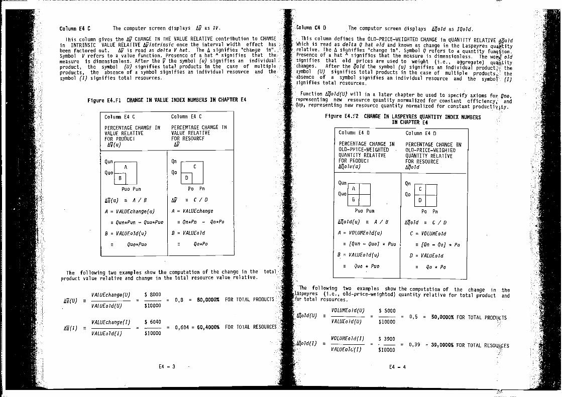
Column E4 C The computer screen displays AV as IV.
This column gives the Aj7 CHANGE IN THE VALUE RELATIVE contribution to CHANGEin INTRINSIC VALUE RELATIVE Aj7intrinsic once the interval width effect has
been factored out. Aj7 is read as delta V hat. The A signifies change in.Symbol V refers to a value function. Presence of a hat signifies that themeasure is dimensionless. After the ji the symbol (u) signifies an individualproduct, the symbol (U) signifies total products in the case of multipleproducts, the absence of a symbol signifies an individual resource and thesymbol (I) signifies total resources.
Column E4 C Column E,4 C
PERCENTAGE CHANGE IN PERCENTAGE CHANGE INVALUE RELATIVE VALUE RELATIVEFOR PRODUCT FOR RESOURCE
AV(u) Al?
QunA
Quo
Puo Pun
a A/BA = VALUEchange(u)
a Qun*Pun — Quo*Puo
B = VALUEo1d(u)
a Quo*Puo
QnC
Qo
P0 Pn
a C/B
A = VALUEchange
a Qn*Pn — Qo*Po
B = VALUEo1d
a Qo*Po
The following two examples show the computation of the change in the totalproduct value relative and change in the total resource value relative.
VALUEchange(U) $ 8000AV(U) a =
______
= 0,8 = 80,0000% FOR TOTAL PRODUCTS
VALUEo1d(U) $10000
VALuEchange(I) $ 6040AV(I) a =
______
= 0,604 = 60,4000% FOR TOTAL RESOURCES
VALUE01d(I) $10000
Column C4 0 The computer screen displays as IQold.
This column defines the OLD—PRICE—WEIGHTED CHANGE in QUANTITY RELATIVE goldwhich is read as delta Q hat old and known as change in the Laspeyres::lative. The A signifies change in. Symbol Q refers to a quantityPresence of a hat A cignifies that the measure is dimensionless. The oldsignifies that old prices are used to weight (i.e., aggregate) quaqtitychanges. After the Qold the symbol (u) signifies an individual product; thesymbol (U) signifies total products in the case of multiple products; theabsence of a symbol signifies an individual resource and the symbol (I)signifies total resources.
will in a later chapter be used to specify axioms fort Qne,representing new resource quantity normalized for constant andQnp, representing new resource quantity normalized for constant productivity.
Figure CHANGE IN LASPEYRES QUANTITY INDEX NUMBERSIN CHAPTER E4
Col umii E4 0 Col umn E4 D
PERCENTAGE CHANGE IN PERCENTAGE CHANGE INOLD—PFflCE—.WEIGHTED OLD—PRICE—WEIGHTEDQUANTiTY RELATIVE QUANTITY RELATIVEFOR PEODUCT FOR RESOURCE
QunM
Quo
B
Puo Pun
A
a
B =
a Quo*Puo
Qn
C
Qo
D
Po Pn
a C / B
C = VOLUMEo1d
a (Qn — Qo] * Po
B = VALUEo1d
a Qo*Po
The following two examples showpeyres (i.e., old—price—weighted)total resources
VOLUMEo1d(U) $ 5000a
____________
=
______
= 0,5 = 50,0000% FOR TOTAL PRODUCTSVALUE01d(U) $10000
Figure E4.F1 CHANGE IN VALUE INDEX NUMBERS IN CHAPTER E4
the computation of the change in thequantity relative for total product and
E4 — 3
VOLUMEo1d(I) $ 3900a =
______
= 0,39 = 39,0000% FOR TOTALVALUEo1cJ(f) $10000
E4 — 4
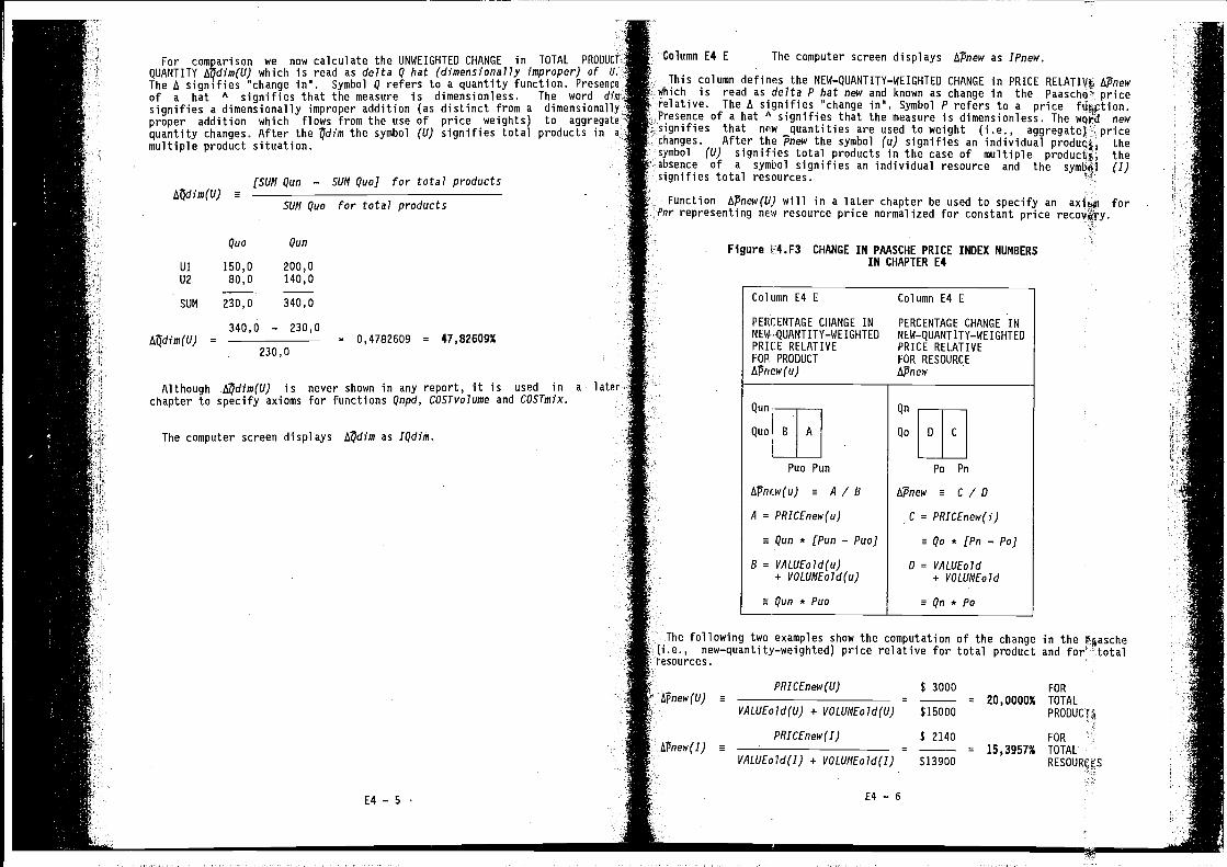
Quo Quo
UI 150,0U2 80,0
SUM 230,0
340,0 — 230,0=
______________
230,0
Column E4 EFor comparison we now calculate the UNWEIGHTED CHANGE in TOTAL PRODUCT
QUANTITY which is read as delta Q hat (dimensionally improper) of U.,The A signifies "change in". Symbol Q refers to a quantity function. Presenceof a hat A signifies that the measure is dimensionless. The word dimsignifies a dimensionally improper addition (as distinct from a dimensionallyproper addition which flows from the use of price weights) toquantity changes. After the the symbol (U) signifies total products in a
multiple product situation.
(SUM Quo — SUM Quo] for total products
SUM Quo for total products
200,0140,0
340,0
The computer screen displays LCpnew as IPnew.
This column defines the NEW—QUANTITY—WEIGHTED CHANGE in PRICE APnewwhich is read as delta P hat new and known as change in the pricerelative. The A signifies "change in". Symbol P refers to a pricePresence of a hat A signifies that the measure is dimensionless. The word newsignifies that nrw quantities are used to weight (i.e., aggregate). pricechanges. After the Pnew the symbol (u) signifies an individual thesymbol (U) signifies total products in the case of multiple theabsence of a symbol signifies an individual resource and the (I)signifies total resources.
Function APnew(U) will in a later chapter be used to specify an forPnr representing new resource price normalized for constant price recovjry.
Figure V4.F3 CHANGE IN PAASCHE PRICE INDEX NUNBERSIN CHAPTER E4
= 0,4782609 = 47,82609%
Although is never shown in any report, it is used in a laterchapter to specify axioms for functions Qnpd, COSTvolume and CQSTmix.
The computer screen displays I4dim as IQdiin.
Column E4 E Column E4 E
PERCENTAGE CHANGE IN PERCENTAGE CHANGE INNEW—QUANTITY—WEIGHTED
PRICE RELATIVE PRICE RELATIVEFOR PRODUCT FOR RESOURcEAPnew(u) APnew
Quo
A
Puo Pun
APncw(u) e A/BA = PRICEnew(u)
aQun*(Pun—Puo]
B = VALUEo1d(u)i- VOLUMEo1d(u)
sQun*Puo
Qn
Qo 0 C
Po Pn
APnew a C/BC = PRICEnew(i)
eQo*(Pn—Po]
B = VALUEo1d+ VOLUMEo1d
aQn*Po
The following two examples show the computation of the change in the(i.e., new—quantity—weighted) price relative for total product andresources.
PRICEnew(U) $ 3000 FORAPnew(U) e
__________________________
=
______
= 20,0000% TOTALVALUEo1d(U) + VOLUME01d(U) $15000
PRICEnew(I) $ 2140 FORàVnew(I) e
__________________________
=
______
= 15,3957% TOTALVALUEoJd(I) + VOLUME01d(I) $13900 RESOURCES
E4—5 E4—6
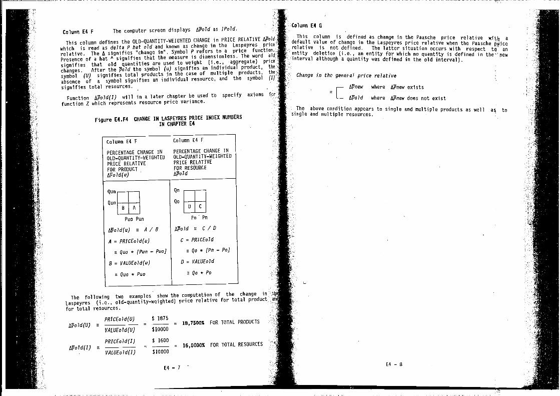
Column E4 F The computer screen displays Aflold as IPold.
This column defines the OLD_QUANTITY—WEIGHTED CHANGE in PRICE RELATIVE IsPold
which is read as delta P hat old and known as change in the Laspeyres price
relative. The A signifies "change in". Symbol P refers to a price function.
Presence of a hat A signifies that the measure is dimensionless. The word ol
signifies that old quantities are used to weight (i.e., aggregate) pr
changes. After the the symbol (u) signifies an individual product,
symbol (U) signifies total products in the case of multiple products,
absence of a symbol signifies an individual resource, and the symbol
signifies total resources.
Function APold(I) will in a later chapter be used to specify axioms
function Z which represents resource price variance.
Figure E4.F4 CHANGE IN LASPEYRES PRICE INDEX NIJNBERSIN CHAPTER E4
Column E4 G
This column is defined as change in the Paasche price relative with adefault value of change in the Laspeyres price relative when the Paascherelative is not defined. The latter situation occurs with respect tq anentity deletion (i.e., an entity for which no quantity is defined in pewinterval although a quantity was defined in the old interval).
APnew where Kflnew exists
where /fPnew does not exist
The above condition appears to single and multiple products as well as tosingle and multiple resources.
Change in the genera! price relative
Column E4 F Column E4 F
PERCENTAGE CHANGE INOLD_QUANTITY—WEIGHTEDPRICE RELATIVEFOR RESOURCEAPold
PERCENTAGE CHANGE INOLD_QUANTITY—WEIGHTEDPRICE RELATIVEFOR PRODUCTAPold(u)
Qun
QuoB A
Puo Pun
APold(u) a A / B
A = PRICEoId(u)
a Quo * (Pun —
Po Pn
APold a C/DC = PRICEoJd
a Qo * (Pn — Po]
B = VALUE0Id(u) D = VALUEoId
aquo*PUo aQo*Po
The following two examples show the computation of the change in
Laspeyres (i.e., old_quantity—weighted) price relative for total product ai
for total resources.
PRICE01d(U) $ 1875APold(U) a =
______
= 18,7500% FOR TOTAL PRODUCTS
VALUE01d(U) $10000
PRICEo1d(I) $ 1600APold(I) a =
______
= 16,0000% FOR TOTAL RESOURCES
VALUE01d(I) $10000
E4—7 -E4 — B
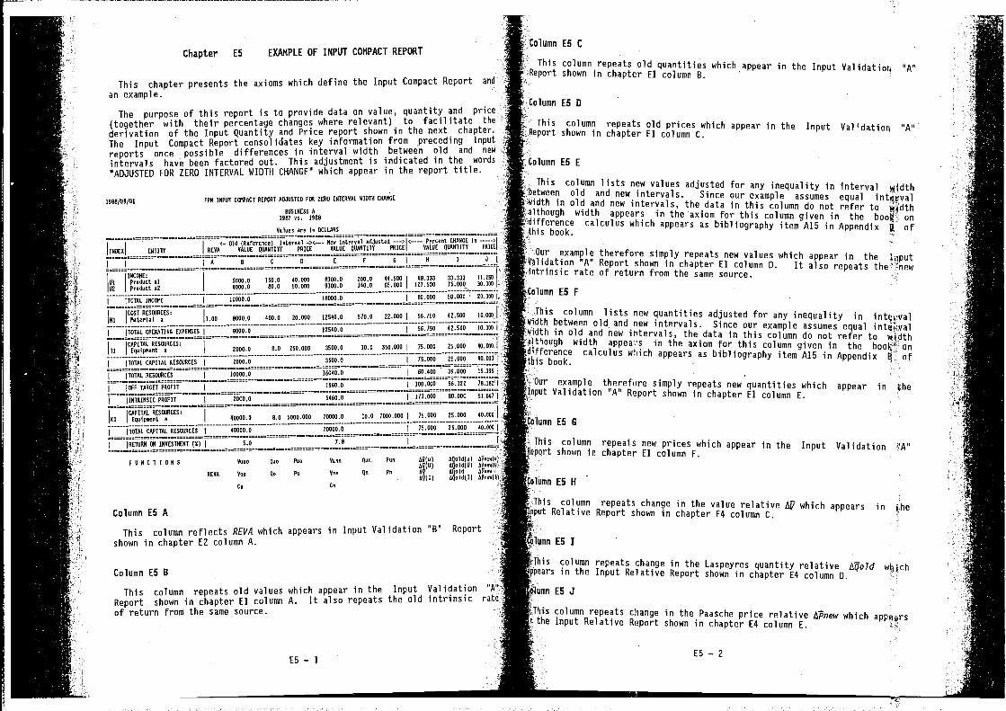
Chapter E5 EXAMPLE OF INPUT COMPACT REPORT
This chapter presents the axioms which define the Input Compact Report and
an example.
The purpose of this report is to provide data on value, quantity and price(together with their percentage changes where relevant) to facilitate the
derivation of the Input Quantity and Price report shown in the next chapter.The Input Compact Report consolidates key information from •preceding Input
reports once possible differences in interval width between old and new
intervals have been factored out. This adjustment is indicated in the words
"ADJUSTED FOR ZERO INTERVAL WIDTH CHANGE" which appear in the report title.
1968/09/01 FPM INPAT COMPACT REPOUT ADJuSTED 1042 ZERO INTERVAL WIDTH CHANGE
90516055 A1987 as. 1988
Values are On COLLARS
c. Old (Reference) Interval —no——— New Interval adjusted ——— <———— Percent tRANCE In
INDEX ENTITY REVA VALRE QUANTITY PRICE VALUE QUANTITY PRICE VALVE QUANTITY PRICE
IN 8 C 0 0 F 6) 8 1 JI
INCORE:RI Product al 6000.9 150.9 40.000 8900.0 200.0 44.100 48.333 33.333 11.210
92 Product a2 4000.0 80.0 10.000 9100.0 140.0 61.000 127.500 75.000 30.000
TOTAL INC04IE 10000.8 10000.0 80.000 10.000 20.000
COST RESOURCES:
NI Materiel a 1.00 8000.0 400.0 20.000 12540.0 510.2 22.000I
56.750 42.500 10.000
(TRIAL OPERATING EXPENSES 8000.0 12540.0 (50.750 42.500 10.000
CA;ITAL RESOURCES: - --TI Equiposent a 2000.0 8.0 200.000 3100.0 10.0 310,000
I
75.OAO 25.000 00.000
(TOTAL CAPITAL RESOURCES 2000.9 3500.0 (75.000 25.000 40
(TOTAL RESOURCES )10000.0 16040.0 60.400 39.000 28.1
(OFF TAROET PROFIT 2960.0 )100.000 06.122 78.1
(INTRINSIC PROFIT — - 2000.0 — 5460.0 —— )173.000 80.000
CAPITAL RESOURCES:
UI Eqaipment a 4OOUO.0 8.0 5OU0.000 70000.0 20.0 7000.000(
75.OUO 25.000 40.000
(TOTAL CAPITAL RESOURCES 40000.0 70000.0 75.000 25.000 40.000
)RETOAN 044 IHAESTNENT (5) 5.0 7.8 I
PUNt 79860 Ruse Ion Poe Vunn Run Pun
ROVA You Re Pe Ann Qn Fn
Ce Cn
Column E5 A
This column reflects REV/I which appears in Input Validation 0B'shown in chapter E2 column A.
Column E5 B
This column repeats old values which appear in the Input Validation °A"
Report shown in chapter El column A. It also repeats the old intrinsic rate!
of return from the same source.
This column lists new values adjusted for any inequality in Interval widthoetween old and new intervals. Since our example assumes equal intai)ovalwidth in old and new intervals, the data in this column do not refer to widthalthough width appears in the axiom for this column given in the ondifference calculus which appears as bibliography item A15 in Appendix a ofu)s book.
Our example therefore simply repeats new values which appear in the iv-,putTlidation Report Shown in chapter El column 0. It also repeatsthe same source.
This column lists new quantities adjusted for any inequality in intervalbetween old and new intervals. Since our example assumes equalin in this column do not refer to wtdthlthough width appears in the axiom for this column given in the boot onlifference calculus which appears as bibliography item A15 in Appendix ofs book.
Our example therefore simply repeats new quantities which appear in:t Validation Report shown in chapter El column E.
E5 G
column repeats new prices which appear in the Input Validationeport shown in chapter El column F.
lumn ES H
TiS column repeats change in the value relative Aj7 which appears in theit Relative Report shown in chapter E4 column C.
imn ES I
column repeats change in the Laspeyres quantity relative whichppRars in the Input Relative Report shown in chapter E4 column 0.
iumn ES J
Otis column repeats change in the Paaschm price relative APnew whichpthe Input Relative Report shown in chapter E4 column E.
E5 — 2
This column repeats old quantities which appear in the Input Validatios4 CACshown In chapter El column B.
ES 0
This column repeats old prices which appear in the Input Validation°°"rt shown in chapter El column C
:::i E5 E
'0
'O
Column ES F1!
00(u) UQeld(o(00(0) 000ld(UIàY UQeld09(1) AQnldI2)
Report:4
E5 — 1
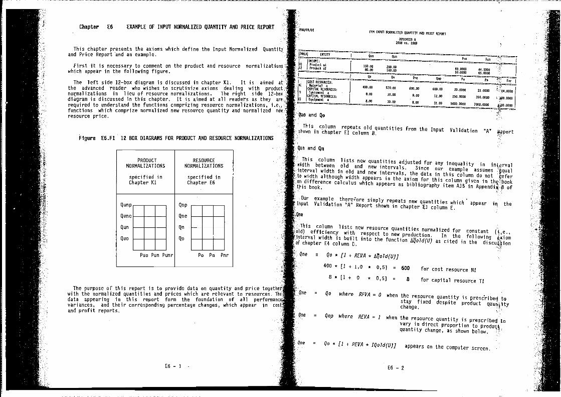
Chapter E6 EXAMPLE OF INPUT NORMALIZED QUANTITY AND PRICE REPORT
This chapter presents the axioms which define the Input Normalized Quantityand Price Report and an example.
First it is necessary to comment on the product and resource normalizationswhich appear In the following figure.
The left side 12—box diagram is discussed in chapter Ki. It is aimed atthe advanced reader who wishes to scrutinize axioms dealing with productnormalizations in lieu of resource normalizations. The right side 12—box
diagram is discussed in this chapter. It is aimed at all readers as they am
required to understand the functions comprizing resource normalizations, i.e.,functions which comprize normalized new resource quantity and normalized new
resource price.
PRODUCT RESOURCE
NORMALIZATIONS NORMALIZATIONS
specified in specified inChapter Ki Chapter E6
Puo Pun Punr Po Pn Pnr
The purpose of this report is to provide data on quantity and price togethwith the normalized quantities and prices which are relevant to resources. Tdata appearing in this report form the foundation of all performanvariances, and their corresponding percentage changes, which appear in c
and profit reports.
IC:
a2150.00 200.0040.00 140.00
I
40.0000 44.500050.0005 05.0000
COSIRESmIRCEST
I Rn Qn Qne Rap, Pu Pn PinI
TI
RI
Material a
CAPITALEquipment a
CAPITALEquipeia,5 a -=
400.00 570.00
4.00 10.00
8.00 10.00
600.00 600.00 20.0000 22.0050 24.0200-
6.00 12.00 250.0005 350.0000 '8.00 12.00 5000.0000 7000.0000
This column lists new quantities adjusted for any inequality in intervalwidth between old and new intervals. Since our example assumes 'equalinterval width in old and new intervals, the data in this column do notwidth although width appears in the axiom for this column given in thç -bookdifference calculus which appears as bibliography item hiS in B of'5 book.
Our example therefore simply repeats new quantities which appear iq the.t Validation cAn Report shown in chapter El column E.
This column lists new resource quantities normalized for constant (I.e.,efficiency with respect to new production. In the following1Mnterval width is buflt into the function as cited in theof chapter E4 column C.
0 Qo * (1 + REVA * I4old(U)]
40D * {l + 1,0 * O,5J = 6OD for cost resource NI8 * [1 + 0 * D,5J = 8 for capital resource Tl
= Qo where REVA = 0 when the resource quantity is presci-ibeci tostay fixed despite product quarqitychange.
= Qnp where REVA = 1 when the resource quantity is prescribed tovary in direct proportion toquantity change, as shown below.
= Qo * (1 + REI'A * IQoldflJ)] appears on the computer screen.
E6 — 2
1988/09/51FPN INPUT NC8IRRLIZEU 5208TITR AND PRICE REPORT
BUSINESS A1988 cm. 1988
Figure E6.F1 12 BOX DIAGRAMS FOR PRODUCT AND RESOURCE NORMALIZATIONS
Quo and Qo
This column repeats old quantitiesshown in chapter El column 8.
and Qn
from the Input Validation cAn
Qne
Qne
E6 — 1
Qne
5-
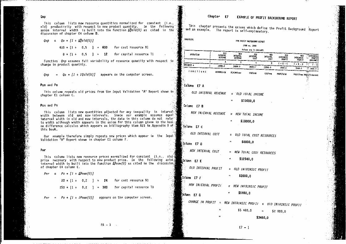
Qnp
This column lists new resource quantities normalized for constant (i.e.,old) productivity with respect to new product quantity. In the followingaxiom interval width is built into the function I4old(U) as cited in thediscussion of chapter E4 column 0.
Qnp a Qo * [1 +
400 * [1 + 0,5 ] = 600 for cost resource NI
8 * [1 + 0,5 1 = 12 for capital resource TI
Function Qnp assumes full variability of resource quantity with respect tochange in product quantity.
Qnp = Qo * (1 + IQold(U)J appears on the computer screen.
Pua and Pa
This column repeats old prices from the Input Validation "A" Report shown inchapter El column C.
Pun and Pn
This column lists new quantities adjusted for any inequality in intervalwidth between old and new intervals. Since our example assumes equalinterval width in old and new intervals, the data in this column do not referto width although width appears in the bookon difference calculus which appears as bibliography item A15 in Appendix B ofthis book.
Our example therefore simply repeats new prices which appear in the InputValidation "A" Report shown in chapter El column F.
Pnr
This column lists new resource prices normalized for constant (i.e.,price recovery with respect to new product price. In the followinginterval width is built into the function APnew(U) as cited in theof chapter E4 column E.
Pnr a Po * [1 + AThiew(U)J
20 * [1 + 0,2 1 = 24 for cost resource Ni
250 * [1 + 0,2 J = 300 for capital resource Tl
For = Po * [1 + IPnew(U,)J appears on the computer screen.
Chapter E7 EXAMPLE OF PROFIT BACKGROUND REPORT
This chapter presents the axioms which define the Profit Background Reportand an example. The report is self—explanatory.
PPM PROFIT O4CK0000RO REPeOT
1988 VS. 1989
are OOLLARO
OPERATICMOLD
ONTEROALMEW
INTERVALOLD
INTERVAL INTERVALMEW INTRINSIC
REVENuE REOENOE
=
COST COSTINIVIN5IC
PVOFOTINTRINSIC PROFIT
morn VARIANCE
F 0 N C T 1 0 9 S REVEROES1d REVENOEVVW COST,]d COSTnew POOFIToSA
E7 A
OLD INTERVAL REVENUE
r_lumn E7 B
PROFITVVW nherent
a OLD TOTAL INCOME
= 110000,0r:.t
'4NEW INTERVAL REVENUE e NEW TOTAL INCOME
= 118000,0
Column E7 C
OLD INTERVAL COST a OLD TOTAL COST RESOURCES
= 18000,0lumn El D
NEW INTERVAL COST = NEW TOTAL COST RESOURCES
= 112540,0Iumn E7 E
OLD INTERVAL PROFIT a OLD INTRINSIC PROFIT
= 12000,0column E7 F
NEW INTERVAL PROFIT a NEW INTRINSIC PROFIT
= 15460,0:olumn El C
CHANGE IN PROFIT = NEW INTRINSIC PROFIT a OLD INTRINSIC PROFIT
$5 460,0— $2 000,0
13460,0
E7 — .1E6—3 -
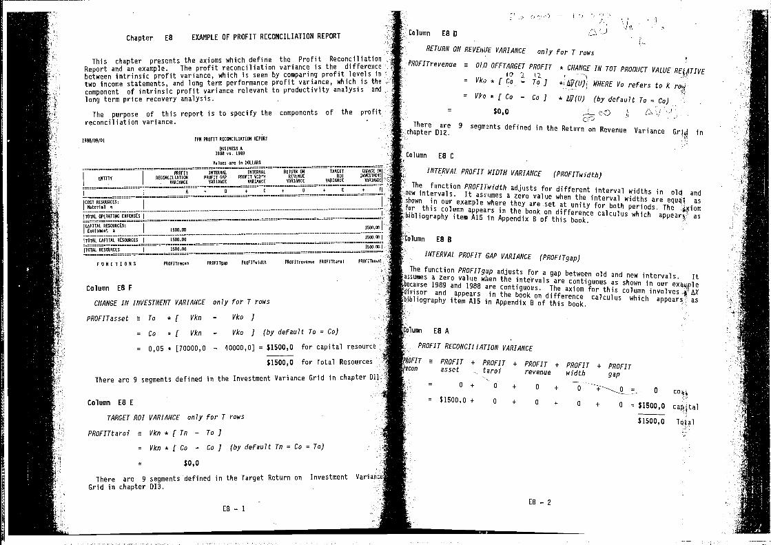
FPM PROFIT RECcNICILIATIOI REPORT
80018050 A1988 vs. 1989
Values are In OOLLARS
/'.i \JA
Chapter E8 EXAMPLE OF PROFIT RECONCILIATION REPORTColumn E8 0
RETURN ON REVEIWE VARIANCE only for T rowsPROFITre venue e 01.0 OFFTARGET PROFIT
10 2 \2= Vko*(Co To]
= Vko*(Co — Co]
There arechapter 012.
Column E8 C
* CHANGE IN TOT PRODUCT VALUE RE4ATIVE
*. AV(U)] WHERE Vo refers to K row
* Aji(U) (by default To =Co)30,0 c±C)
A
9 segments defined in the Return on Revenue Variance in
This chapter presents the axioms which define the Profit ReconciliatiooReport and an example. The profit reconciliation variance is the differencebetween intrinsic profit variance, which is seen by comparing profit levels intwo income statements, and long term performance profit variance, which is thecomponent of intrinsic profit variance relevant to productivity analysis and
long term price recovery analysis.
The purpose of this report is to specify the components of the profitreconcil iation variance.
198 8/09/01
PROFIT INTERVAL INTERVAL RETURN 01 TAREET CVVNSE IN
ENTITY RECENCILIATIEN PROFIT GAP PROFIT 81010 REVENUE RSI IN505TNENI
- - VARIANCE VARIANCE VARIANCE VARIANCE VARIANCE VVRIVNCE
A = 8 + C + U + E +
COST RESOJRCEI:NaEarIal a
ITOTAL OPERATING EVPEVSE5 - —- — - -— -
-I
CAPITAL RESENRCE5:EquVpnenE a 1500.00 1500.01
ITOTAL CAPITAL RESOORCES 1500.001500.00
I
TOTAL RESENRCES 1500.00 1500.00
F 0 N C T I 0 N S PROFITOeCOS PROFITgap PROFITwIdEA
Column E8 F
CHANGE IN INVESTMENT VARIANCE only for T rows
PROFITasset m To * ( Vkn — Vko J
= Co * ( Vkn — Vko ] (by default To = Co)
= 0,05 * [70000,0 — 40000,OJ = 31500,0 for capital resource
$1500,O for Total Resources -.
There are g segments defined in the Investment Variance Grid in chapter 011..
Column EB EI
TARGET ROI VARIANCE only for T rows
PROFITtaroi e Vkn * [ Tn — To ]
PROFITrRve,un PROFITEarOI PROFITa5snI
umn E88
VARIANCE (PROFITwIdt/i)
The function PROFITwidth adjusts for different interval widths in old andnew intervals. It assumes a zero value when the interval widths are aslown in our example where they are.set at unity for both periods. Thethis column appears in the book on difference calculus which asliography item A15 in Appendix B of this book.
INTER VAL PROFIT GAP VARIANCE (PROFITgap)
The function PROFITgap adjusts for a gap between old and new intervals. itsumes a zero value when the intervals are contiguous as shown in our exaooplermIIe 1989 and 1988 are contiguous. The axiom for this columnin the book on difference calculus which as1iography item A15 in Appendix B of this book.
iron E8A
PROFIT RECONCILIATION VARIANCE
a PROFIT + PROFIT + PROFIT + PROFIT + PROFITasset taroi revenue width gap
= 0+ + 0 +
= Vkn * (Co — Co] (bydefault Tn = Co = To)
= $1500,o + 0 +
$0, 0
There are 9 segments defined in the Target Return on Investment Variano
Grid in chapter 013.
£8 — 1
0 cost0 + 0 + 0 = $1500,o capJtaj
$l500,o Tqtal
£8 — 2
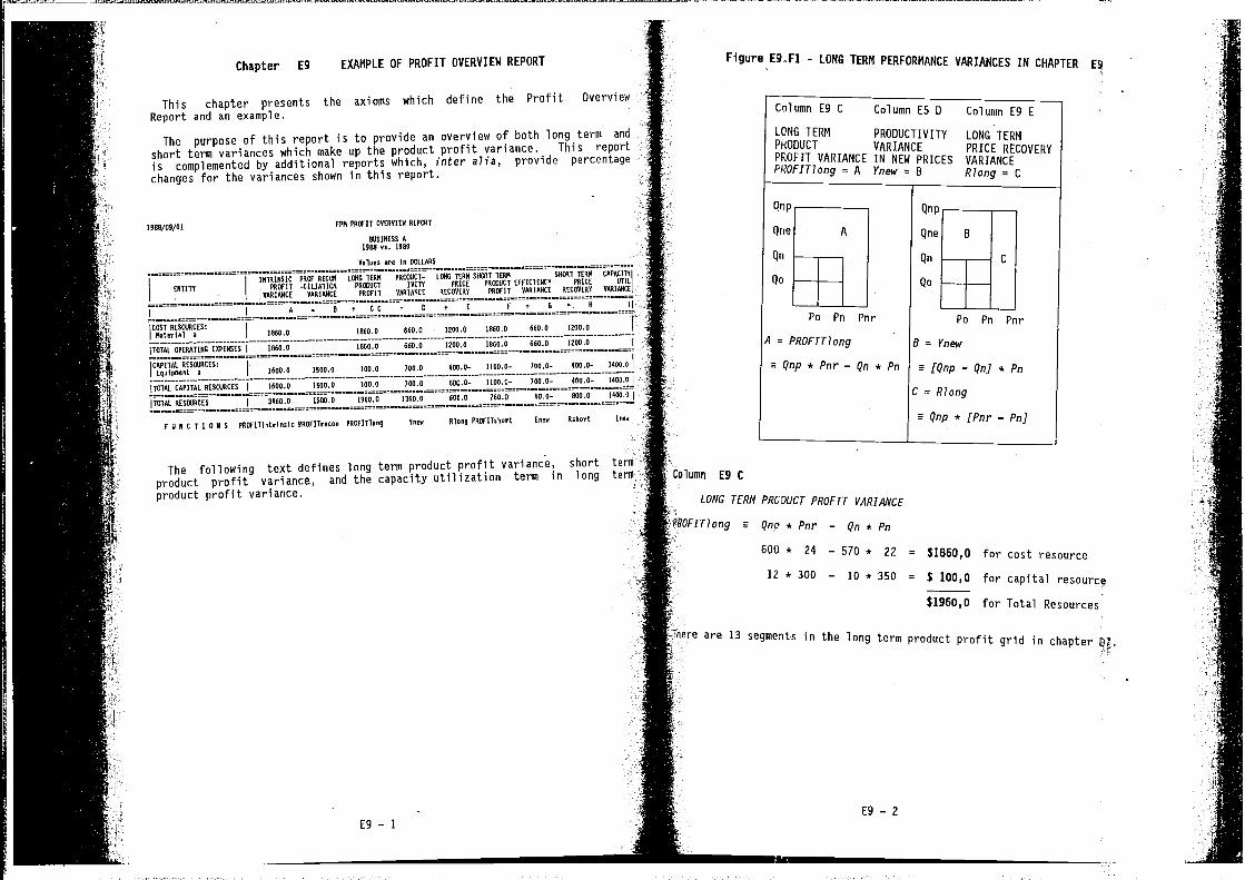
Chapter E9 EXAMPLE OF PROFIT OVERVIEW REPORT
This chapter presents the axioms which define the Profit Overview
Report and an example.
The purpose of this report is to provide an overview of both long term and
short term variances which make up the product profit variance. This report
is complemented by additional reports which, inter a7ia, provide percentage
changes for the variances shown in this report.
1988/09/01 PPM PROFIT OVERVIEW REPa8T
BUSINESS a1980 vs. 1989
Values are in DOLLARS
INTRINSIC PROP REC80 TERN PRODUCT— L880 TERM SHOiT TERM SHORT TERM CAPACITY
ENTITY PRRPIT —dIlATION PRODUCT IRITT PRICE PROEUCT EFFICIENCY PRICE 0Th
VYROUNCE RARIONCE PROFIT RARIARCE RECOVERY PROFIT VARIANCE RECOVERY VARIANCE
U I + CC 0 + E F 0 + 8 Ii
COST REOER1RCES: =
Material a 18600 1860.0 660.0 1l0O.R 1860.0 660.0 1200.0
TOTAL OPERATSNS EXPENSES I1860.0 1860.0 660.0 0200.0 1860.0 660.0 1000.0
CAPITAL RESWRCES:Equipment a —
—— 1600.0 1500.0 100.0 700.0—
608.0: 1100.0— 700.0 — 485.0— 1800.0
TOTAL CAPITAL REOWRCES I1800.0 1100.0 100.0 780.8 800.0— 2180.0— 708.0— 400.0— 1400.0
I
!T0b0. RE501RCES I3000.0 1000.0 1060.8 1360.0 = 680.0 708.0 60.0- 800.0
P 8 N C T I 09 S PROPITintrinsic PROPSTrecon PROFITYOng mew Rlnng PROFIT5VOrC Enen
The following text defines long term product profit variance, short term
product profit variance, and the capacity utilization term in long term
product profit variance.
Figure E9JI - LOMO TERM PERFORMAMCE VARIAMCES IM CHAPTER
Column Eg C Column E5 0 Column E9 E
LONG TERM PR000CTIVITy LONG TERMPI<ODUCT VARIANCE PRICE RECOVERYPROFIT VARIANCE IN NEW PRICES VARIANCEPh'OFIT7ong = A Ynew = B Rlong = C
ES — 1
There are 13 segments in the long term product profit grid in chapter
ES — 2
Po Pn Pnr
A =
a Qnp * Pnr — Qn * Pn
Rshort
Po Pn Pnr
Lena
B = Ynew
[Qnp — Qn] *
C = Riong
a Qnp * (Pnr — Pn]
Column ES C
LONG TERM
rlong a
PRCDUCT PROFIT VARIANCE
Qnc' * Pnr — Qn *
600 * 24 — 570 * 22 = $1860,O for cost resource
12 * 300 — 10 * 350 = $ 100,0 for capital resource
$1960.0 for Total Resources
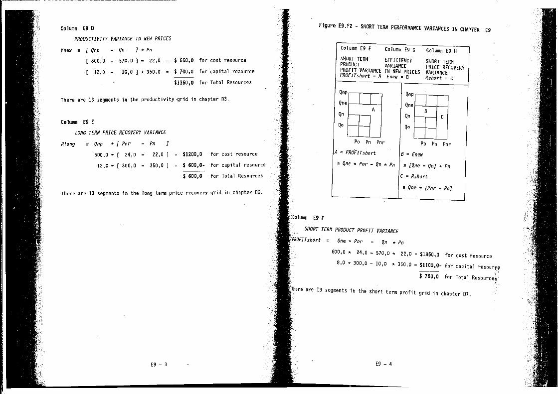
VARIANCE IN NEW PRICES
— Qn 7*Pn
— 570,0 * 22,0 = $ 660,0 for cost resource
— 10,0 3 * 350,0 = $ 700,0 for capital resource
$1360,0 for Total Resources
There are 13 segments in the productivity grid in chapter 03.
Column E9 E
LONG TERM PRICE RECOVERY VARIANCE
Riong a Qnp * [ Pnr — Pn J
600,0 * [ 24,0 — 22,0
12,0 * [ 300,0 — 350,0 3
There are 13 segments in the long term price recovery grid in chapter D6.
Column E9 F
SHORT TERM PRODUCT PROFIT VARIANCE
rlTshort a Qne * Pnr — Qn *
600,0 * 24,0 — 570,0 * 22,0 = $1860,0 for cost resource8,0 * 300,0 — 10,0 * 350,0 $1I00,0- for capital
$ 760,0 for Total Resource
There are 13 segments in the short term profit grid in chapter 07.
Column E9 0
PRODUCTIVITY
Ynew a f Qnp
600,0
12,0
Figure E9.F2 - SHORT TERM PERFORMANCE VARIANCES IN CHAPTER E9
$1200, 0
= $ 600,0-
$ 600,0
for cost resource
for capital resource
for Total Resources
E9 — 3 Eg—4
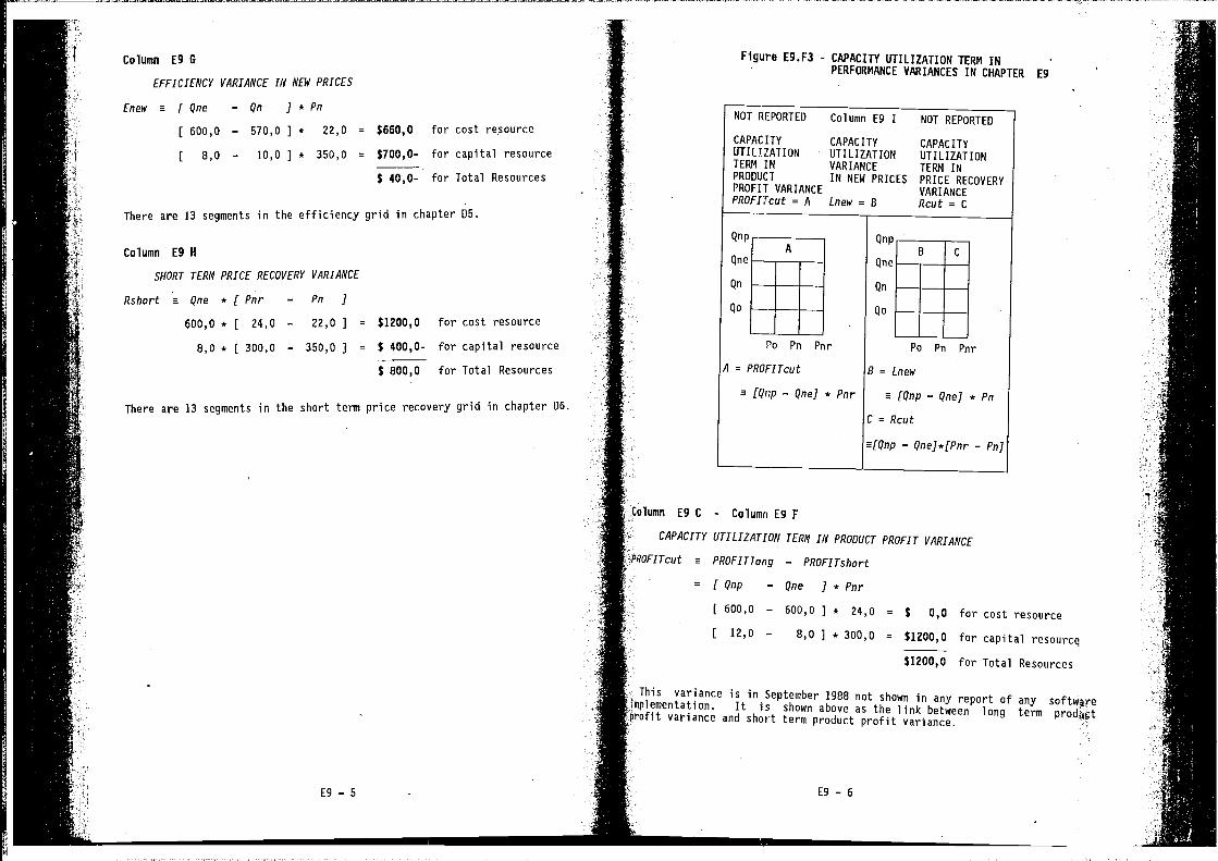
Enew a [ Qne — Qn ] *
600,0 — 570,0 1 * 22,0 = $660,O for cost resource
8,0 — 10,0 ] * 350,0 = $700,0- for capital resource
$ 40,0- for Total Resources
There are 13 segments in the efficiency grid in chapter D5.
Column E9 H
SHORT TERM PRICE RECOVERY VARIANCE
Rshort a Qne * ( Pnr — Pn J
600,0 * [ 24,0 — 22,0 1 =
8,0 * [ 300,0 — 350,0 ] =
There are 13 segments in the short term price recovery grid in chapter D6.
Column E9 C
CAPACITY
PROFITcut a
- Column E9 F
UTILIZATION TERM IN PRODUCT PROFIT VARIANCE
PROFIT1ong — PROFITshort
= (Qnp — Qne ]*Pnr600,0 — 600,0 1 * 24,0 = $ 0,0 for cost resource12,0 — 8,0 ] * 300,0 = $1200,0 for capital resource
$1200,O for Total Resources
This variance is in September 1988 not shown in any report of any softwareimplementation, It is shown above as the link between long termvariance and short term product profit variance.
Column E9 G
EFFICIENCY VARIANCE IN NEW PRICES
Figure E9.F3 - CAPACITY UTILIZATION TERM INPERFORMANCE VARIANCES IN CHAPTER E9
NOT REPORTED Column E9 I NOT REPORTED
CAPACITY CAPACITY CAPACITYUTILIZATION UTILIZATION UTILIZATIONTERN iN VARIANCE TERM INPRODUCT IN NEW PRICES PRICE RECOVERYPROFIT VARIANCE VARIANCEPROFITcut = A Lnew = 8 Rcut = C
$1200,O for cost resource
$ 400,0- for capital resource
$ 800,0 for Total Resources
Pn Pnr P0 Pn Pnr
A = PROFITcut
a [Qnp — Qne] * Pnr
B = Lnew
a(Qnp—Qne]*pp
C = Rcut
a[Qnp — QneJ*(Pnr — Pn]
E9 — 5 [9 — 6
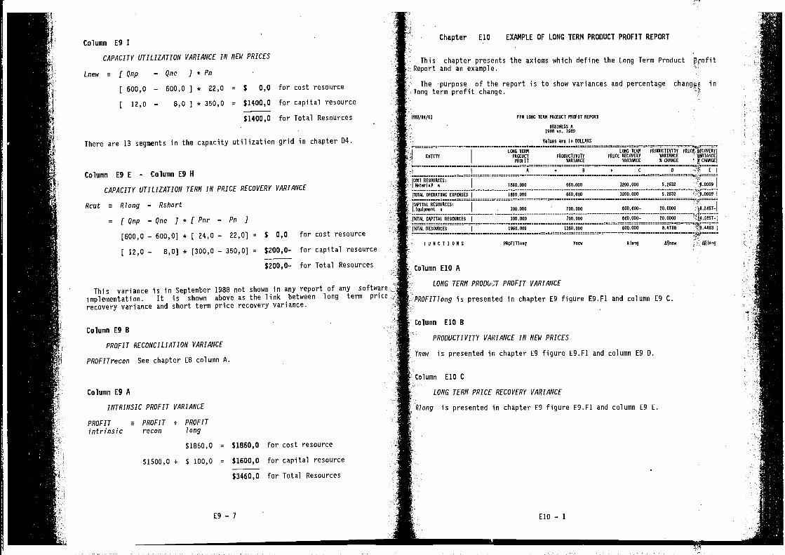
Column E9 I
CAPACITY UTILIZATION VARIANCE IN NEW PRICES
Lnew [Qnp — Qne J*Pn
[600,0 — 600,0] * 22,0 = $ 0,0 for cost resource
12,0 — 8,0 ] * 350,0 = $1400,O for capital resource
$1400,0 for Total Resources
There are 13 segments in the capacity utilization grid in chapter D4.
Column E9 E - Column E9 H
CAPACITY UTILIZATION TERM IN PRICE RECOVERY VARIANCE
Raft a Rlong — Rshort
= fQnp —Qne ] *[Pnr — Pn 3
[600,0 — 600,0] * [ 24,0 — 22,0] = $ 0,0
12,0 — 8,0] * [300,0 — 350,0] = $200,0—
$200,0- for Total Resources
This variance is in September 1988 not shown in any report of any software
implementation. It is shown above as the link between long term pricerecovery variance and short term price recovery variance.
Column E9 B
PROFIT RECONCILIATION VARIANCE
PROFITrecon See chapter E8 column A.
$1850,0 = $1B60,O for cost resource
$1500,0 + $ 100,0 = $1600,0 for capital resource
$3460,0 for Total Resources
Column ElO A
LONG TERM PROOL'JT PROFIT VARIANCE
PROFIT1ong is presented in chapter E9 figure E9.F1 and column E9 C.
Column ElO B
PRODUCTIVITY VARIANCE IN NEW PRICES
Ynew is presented in chapter E9 figure E9.F1 and column E9 0.
Column E1O C
LONG TERN PRICE RECOVERY VARIANCE
is presented in chapter £9 figure E9.F1 and column [9 [.
It Chapter E1O EXAMPLE OF LONG TERN PRODUCT PROFIT REPORT
This chapter presents the axioms which define the Long Term Product PcofitReport and an example.
The purpose of the report is to show variances and percentage inlong term profit change.
988/09/01 FPM LONG TERM PROOIUCT POOFIT REPONT
DUllNESS A1988 v, 1889
Values are I' DOLLARS
for cost resource
for capital resource
ENTITY PRWUCTPROFIT
A
PRONUCTI RIOTVARIANEE
9
powucnvIlTpRicr!kcovEoyPRICE RECOVERY VARIANCE IARIPJXCE
VARIANCE C CVANOE CNAOOE
+ C I) E
COOT RESOUOCES:
Material a 1880.000 660.000 1200.000 9.2632
TOTAL OPERATING EXPENSES 1860.000 660.000 1200.000 9.2032
CAPITAL RESWRCES:!
Equipme'L a 100.000 700.002 600.OSO— 20.0000 14.2857—
FONCTIONS PROFITOsng Ynew bong
A
INTRINSIC PROFIT VARIANCE
PROFIT a PROFIT + PROFIT
intrinsic recon long
4
E9 — 7 £10 — 1
a
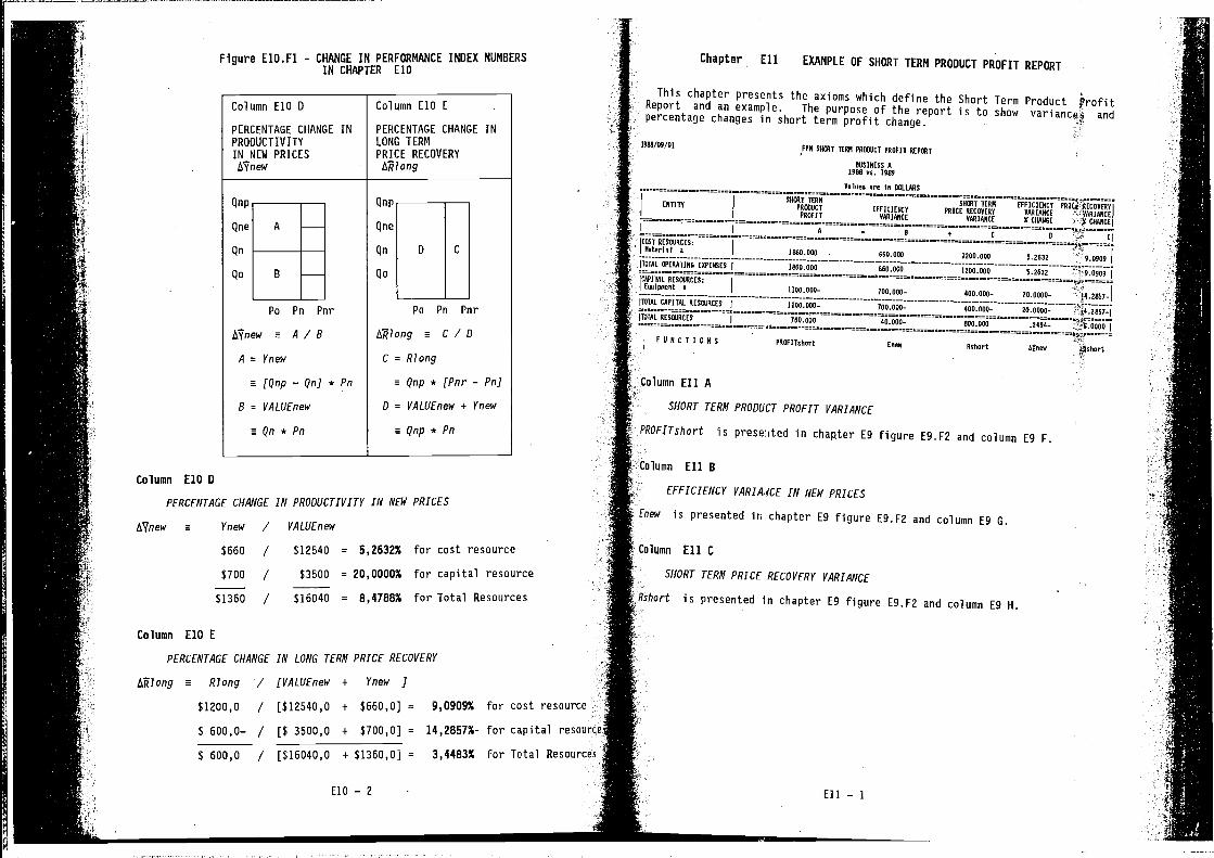
Column ElO D Column E10 E
PERCENTAGE CHANGEPRODUCTIVITYIN NEW PRICES
AVnew
IN PERCENTAGE CHANGE INLONG TERMPRICE RECOVERY
Po Pn Pnr P0 Pn Pnr
A7new a A / B a C / 0
A = Ynew C = Riong
a [Qnp — Qnj * Pn a Qnp * (Pnr — PnJ
B = VALUEnew 0 = VALUEnew + Ynew
mQn*Pn mqnp*Pn
Qnp
Qne
Qn
Qo
Column ElO D
PERCENTAGE CHANGE IN PRODUCTIVITY IN NEW PRICES
a Ynew / VALUEnew
$660 / $12540 = 5,2632% for cost resource
$700 / $3500 = 20,0000% for capital resource
$1360 / $16040 = 8,4788% for Total Resources
Column ElO E
PERCENTAGE CHANGE IN LONG TERM PRICE RECOVERY
a Riong / (VALUEnew + Ynew 3
$1200,O / [$12540,0 +
$ 600,0— / [$ 3500,0 +
$ 600,0 / [$16040,O +
Column Eli A
SHORT TERM PRODUCT PROFIT VARIANCE
PROFITshort is prese:ited in chapter E9 figure E9.F2 and column E9 F.
EFFICIENCY VARIAICE IN NEW PRICES
is presented in chapter E9 figure E9.F2 and column E9 G.
lumn Eli C
SHORT TERM PRICE RECOVERY VARIANCE
,lort is presented in chapter E9 figure E9.F2 and column E9 H.
Figure E10.Fi - CHANGE IN PERFORMANCE INDEX NUMBERSIN CHAPTER ElO
Chapter Eli EXAMPLE OF SHORT TERM PRODUCT PROFIT REPORT
This chapter presents the axioms which define the Short Term Product profitReport and an example. The purpose of the report is to show andpercentage changes in short term profit change.
rPM SHOUT TERN PROUUCI PROFIT REPOUT
NOSINESS A1988 vs. 1989
Values are In DOLLARS
ENTITYPROSUCT EFFICIENCY PRICE RECOVERY VARIANCE VARIANCEPROFIT VARIANCE VARIANCE % CWINGE CROSGE
COST RESOURCES:Material a 1800.000 660.000 1200.001 5.2632 ' 9.0909
TOTAL OPERATING EXPENSESI — — 1860.000 660.000 — 1200.000 5.2832
Equlpi,ent a 1100.000- 700.000— 400.000— 20.6000-TOTAL CAPITAL RESOURCES
I 1100.000- 700.000— 406.000—
J4.2857_
20.0000—TOTAL RESOURCES
J 760 000 48 000 900 000 2494— p5
0000I
hurt
$660,O] = 9,0909% for cost resource
$700,0] = 14,2857%- for capital resourc
$1360,O] 3,4483% for Total
ElO — 2 Eli — 1
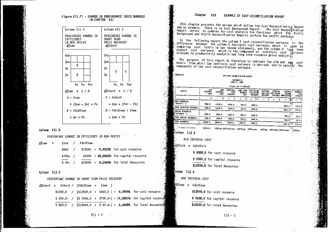
Chapter E12 EXAMPLE OF COST RECONCILIATION REPORT
This chapter presents the axioms which define the Cost ReconciliatitrnReportand an example. There is no Cost Background Report. The Cost ReconcfliationReport serves to combine for cost analysis the functions which ProfitBackground and ProFit Reconciliation Reports perform for profitIn the following report the column E cost reconciliation variance is thedifference between the column C intrinsic cost variance, which is seen bycomparing cost levels in two income statements, and the column D termproduct cost variance, which is the component of intrinsic cost Oriancerelevant to productivity analysis and long term resource price
The purpose of this report is therefore to indicate the old and costlevels from the intrinsic cost variance is derived, and to spec{fy thecomponents of the cost reconciliation variance.
C 5 4 EE P 4 + + I,
8000.0 12510.0 4540.0— 540.0— 4000.0— 3826.1— 173.9—EXPENSES
I0000.0 12540.0 4540.0— 540.0— 4000.0— 3026.1' 173.9—p
L
2000.0 3500.0 1520.0- 500.0- 1000.0- 43.5-I 2000.0 3500.0 1500.0— 500.0— 1000.0— oso.o:I 10000.0 16040.0 6040.0— 1040.0— 5000.0—
217.4_I
Figure EI1.F1 - CHANGE IN PERFORMANCE INDEX NUMBERSIN CHAPTER Eli
Column Eli D Column Eli E
PERCENTAGE CHANGEEFFICIENCYIN NEW PRICESlsrnew
IN PERCENTAGE CHANGE INSHORT TERMPRICE RECOVERY
Po Pn Pnr Po Pn Pnr
AEnew a A/BA C = Rshort
a(Qne—QnJ*Pn aqne*[Pnr—Pn]
B = VALUEnew U = VALUEnew + Enew
aqn*pn aQne*Pn
ENTITY
PPM COST RECONCILIATION REPLO2T
BUSINESS A2988 vs. 1989
Values are In DOLL000
OLD NEW INTRINSIC LONG TERN COST RECLOI INTERVAL INTERVAL P0000CTINTERVAL INTERVAL COST PROSUCT -CILIOTION COST GAP COST WIDTH 0010MW MbCOST COOT VARIANCE COST WAOIANCE VARIANCE VARIANCE ONVEIOVTEP EFrECTA — I
Column Eli 0
PERCENTAGE CHANGE IN EFFICIENCY IN NEW PRICES -
Atnew a Enew / VALUEnew
$660 / $i2540 = 5,2632% for cost resource
$700— / $3500 = 20,0000%- for capital resource
$ 40— / $16040 = 0,2494%- for Total Resources
Column Eli E
PERCENTAGE CHANGE IN SHORT TERN PRICE RECOVERY
a Rshort / (VALUEnew + Enew
$1200,0 / [$12540,O + $66O,0 ] = 9,0909% for cost resource! I
$ 400,0— / [$ 3500,0 ÷ $700,O—] = 14,2857%— for capital resoUA
$ 800,0 / [$16040,0 + $ 40,0—] = 5,0000% for Total Resoun
ElI — 2
1';P U N C T I 0 N S CGSTo1d COOTnee COSTintrinsIc COST9ong COSTrecon COSTgap COSTWIdEN COSTyolume
:olumn E12 A
OLD INTERVAL COST
'OSTo7d a VALUEO !L1
$ 8000,0 for cost resource
$ 2000,0 for capital resource
$l0000,0 for Total Resources
E12 8
NEW INTERVAL COST
OSTnew a VALUEnew
$12540,O for cost resource
$ 3500,0 for capital resource
$16040,O for Total Resources
E12 — I
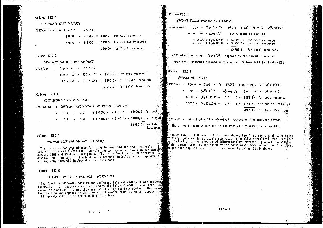
Column E12 C
INTRINSIC COST VARIANCE
COSTintrinsic a COSTa1d
$8000
$2000
Column E12 D
LONG TERM
COST1ong a
= 5540,0- for cost resource
= $500,0- for capital resource
$1040,0- for Total Resources
VARIANCE
COSTwidth + COSTv0 lame + COSTmIx
= 0,0 + 0,0 + 53826,1— + 5173,9— = 54000,0- for cost
= 0,0 + 0,0 + $ 956,5— + $ 43,5— = 51000,0- for capi
$5000.0- for Total
(see chapter E4 page 5)
= 53826,1- for cost resource= $ 956,5- for cost resource
$4782,6- for Total Resources
appears on the computer screen.
the Product Volume Grid in chapter 011.
COSTmIx a (Qnpd — QnpJ * Pa WHERE Qnpd = Qa * (1 + Mdim(U)J
= Va * — (see chapter £4 page 5)
$8000 * [0,4782609 — 0,5 ] = $173.9- for cost resource
$2000 * [0,4782609 — 0,5 = $ 43,5- for capital resource
5217,4- for Total
= Va * (IQdim(U) — IQold(U)J appears on the computer screen.
There are 9 segments defined in the Product Mix Grid in chapter Dli.
Column E12 F
INTERVAL COST GAP VARIANCE (COSTgap)
The function COSTgap adjusts for a gap between old and new intervals.assumes a zero value when the intervals are contiguous as shown in our examibecause 1989 and 1988 are contiguous. The axiom for this column involves adivisor and appears in the book on difference calculus which appears
bibliography item AlS in Appendix B of this book.
Column E12 8
INTERVAL COST WIDTH VARIANCE (COSTwidth)
The function COSTwidth adjusts for different interval widths in old andintervals. It assumes a zero value when the interval widths are equal
shown in our example where they are set at unity for both periods. The axi,
for this column appears in the book on difference calculus which appears
bibliography item A15 in Appendix B of this book.
E12 — 2
In columns £12 H and E12 I shown above, the first right hand expresstonsy Qnpd which represents new resource quantity normalized for
ductivity using unweighted (dimensionally improper) product quantities..s composition is indicated by the constraint shown alongside the fft-st
.'ight hand expression of the axiom covered by column £12 H above.
El? — 3
— COSTnew
— $12540 =
— $ 3500 =
$4540- for cost resource
$1500- for capital resource
$6040- for Total Resources
= — Vo * I4dim(U)
— $8000 * 0,4782609— $2000 * 0,4782609
PRODUCT COST VARIANCE
Qnp*Po — Qn*Pn
600 * 20 — 570 * 22
12*250 — 10*350
Column E12 H
PRODUCT VOLUME UNWEIGHTED VARIANCE
COSTvolame m [Qo — Qnpd] * Pa where Qnpd = Qo * (1 +
COSTvo lame = — Va * IQdim(U)
There are 9 segments defined in
E12 I
PRODUCT MIX EFFECT
Column El? E
COST RECONCILIATION
COSTrecon a COSTgap +
I
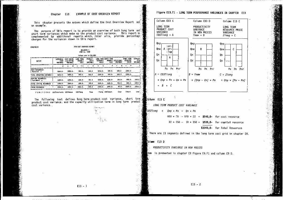
Chapter E13 EXAMPLE OF COST OVERVIEW REPORT
This chapter presents the axioms which define the Cost Overview Report and
an example.
The purpose of this report is to provide an overview of both long term and
short term variances which make up the product cost variance. This report iscomplemented by additional reports which, inter al/a, provide percentagechanges for the variances shown in this report.
1988/AM/Al PPM COST OREORSEA AEPCIOT
BUSINESS A1000 vs. 1818
— -—— Aalues are In DOLLARS
IN001MSIC COST 8ECOS LOSS TERN PROSUCT— 1880 TEAM SMOST TERM SAOTT TEAM CI
ENTITY COST -CILIATImI PRCOOCT TASTY AESmIACE P0000CT EFFICIENCY AESC4JACE
AURSYACE AmBIANCE COST AmBIANCE PRICE COST AAAIUNCE PAICE RI
A • B 4 CC D + E F 0 + A
COST RE5000CES:Material a 0540.0— AOOS.O— SASS— 080.0 1200.0— 540.0— 080.0 1200.0—
TOTAL OPERATING EUPEASES 454A.O- 4000.0- 540.0- 1000.0- 540.0- 080.0 1000.0-
CAPITAL RE5008CES:Equipiavnt a ISSO.0— 1000.0— 500.0— 700.0 1200.0— 1500.0— 700.0— 800.0— 1400.0
ITOTAL CAPITAL RE500RCES I1500.0— 1000.0— 500.0— 700.0 0200.0- 1500.0- 700.0— 800.0- 140011
ITOTAL RE5008CES = 8040.0— 5000.0— ;OAO.T 1380.0 2400.0— SOAO.O— AO.O— 2000.0— lASSOI
F 0 8 C T I 0 N S COSTT,trI,slc COSTrecon COSTlong Once Zlong COSTohorL
The following text defines long term product cost variance, short termproduct cost variance, and the capacity utilization term in long term productcost variance.
Cumn E13
LONG TERM PRODUCT COST VARIANCE
Qnp * Po — Qn * Pn
600 * 20 — 570 * 22 = $54O,O- for cost resource
12 * 250 — 10 * 350 = $500,O- for capital resource
$IO4O,O- for Total Resources
There are 13 segments defined in the long term cost grid in chapter DY.
Figure E13.F1 - LONG TERM PERFORMANCE VARIANCES IN CHAPTER E13
A
Column E13 C Column E13 D Column E13 E
LONG TERM PRODUCTIVITY LONG TERMPRODUCT COST VARIANCE RESOURCE PRICEVARIANCE IN NEW PRICES VARIANCECOSTlong = A Ynew = B Zlong = C
Po Pn Prir
= COSTlong
e Qnp * Po — Qn * Pn
=B÷C
Po Pn Pnr Po Pn Pnr
B = Ynew C = Zlong
(Qnp — QnJ * Pn m Qnp * [Po — PnJ
Enow 0 short Lnoo
m
E13 — I
PRODUCTIVITY VARIAMCE IN NEW PRICES
is presented in chapter E9 figure E9.F1 and column E9 0.
E13 — 2
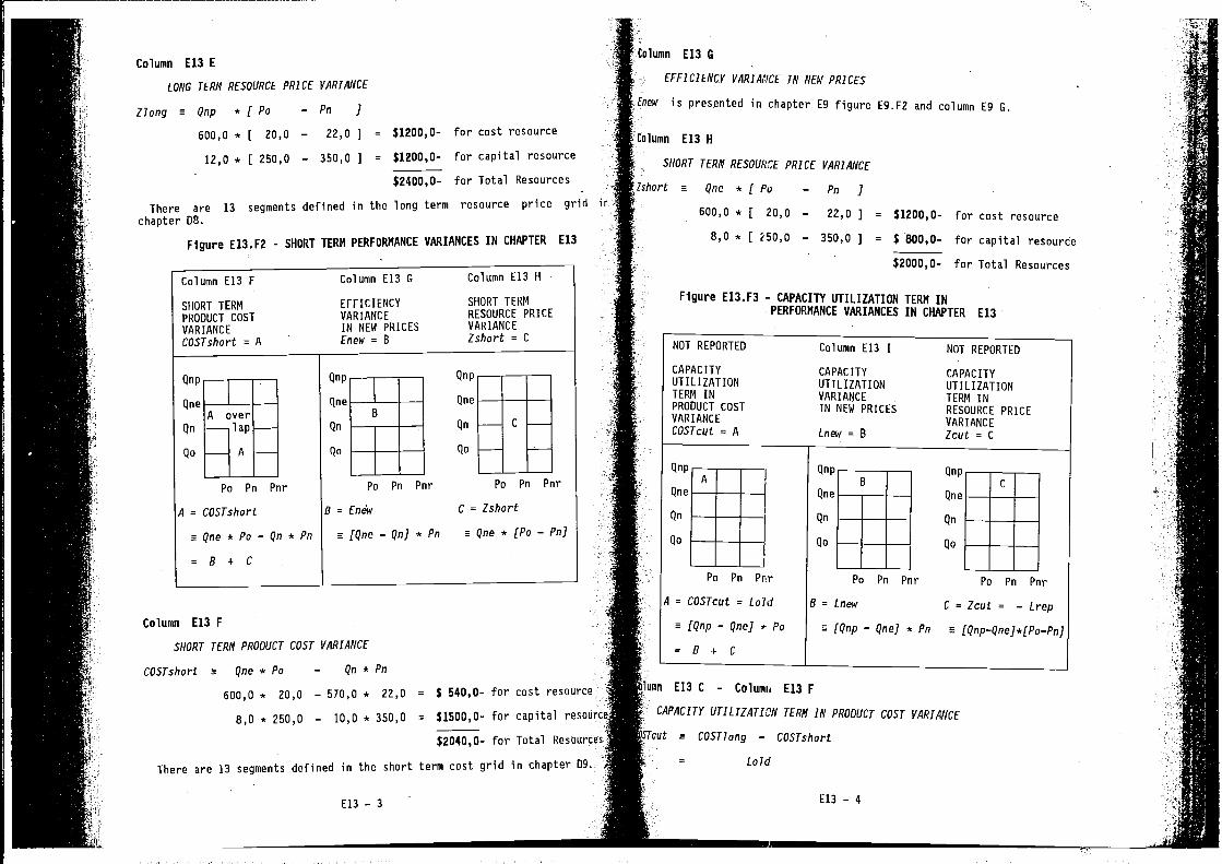
TERM RESOURCE PRICE VARIANCE
Qnp *[Po — Pn ]600,0 * [ 20,0
12,0 * [ 250,0
Column E13 F Column E13 G Column E13 H
SHORT TERM EFFICIENCY SHORT TERM
PRODUCT COST VARIANCE RESOURCE PRICE
VARIANCE IN NEW PRICES VARIANCE
COSTshort = A Enew = B Zshort = C
Qnp1
QneA over
P0 Pn Pnr
A = COsTshort
Qne * Pa — Qn * Pn
=B+C
Qnp Qnp
Qne Qne
B
C
Pa Pn Pnr P0 Pn Pnr
B = C = Zshort
(Qne — Qnj * Qne LP0 — PnJ
Column E13 F
SHORT TERM PRODUCT COST VARIANCE
COSTshort Qne * Pa — Qn *
600,0 * 20,0 — 570,0 * 22,0 = $ 540,0- for cost resource I8,0 * 250,0 — 10,0 * 350,0 = $1500,0- for capital
$2040,0- for Total Resources
There are 13 segments defined in the short term cost grid in chapter 09.
E13—3
E13 G
EFFICIENCY VARIAPCE IN NEW PRICES
is presented in chapter E9 figure E9.F2 and column E9 G.
SHORT TERM RESOURCE PRICE VARIANCE
Qne * [ Pa — Pn .1
600,0 * [ 20,0 — 22,0 1
8,0 * [ 250,0 — 350,0 1
Iumn E13 C - Columi, E13 F
CAPACITY UTILIZATION TERM IN PRODUCT COST VARIANCE
COSTiang — CO5Tshort
Column E13 E
LONG
Ziong
There are 13 segmentschapter 08.
— 22,0 ] = $1200,O- for cost resource
— 350,0 ] = $1200,0- for capital resource
$2400,0- for Total Resources
defined in the long term resource price grid in
Figure E13.F2 - SHORT TERM PERFORMANCE VARIANCES IN CHAPTER E13
= $1200,0- for cost resource
= $ 800,0- for capital resource
$2000,0- for Total Resources
Figure E13.F3 - CAPACITY UTILIZATION TERM INPERFORMANCE VARIANCES IN CHAPTER E13
NOT REPORTED Column E13 I NOT REPORTED
CAPACITY CAPACITY CAPACITYUTILIZATION UTILIZATION UTILIZATIONTERM IN VARIANCE TERM INPRODUCT COST IN NEW PRICES RESOURCE PRICEVARIANCE VARIANCECOSTcut = A Lnew = B Zcut = C
Po Pn Pnr
A = COSTcut = Loid
a [Qnp — Qne] * Pa
=B+C
Pa Pn Pnr Po Pn Pnr
B = Lnew C = Zcut = — Lrep
(Qnp — Qne] * Pn a (Qnp—Qne]*(Po—PnJ
Laid
E13 — 4
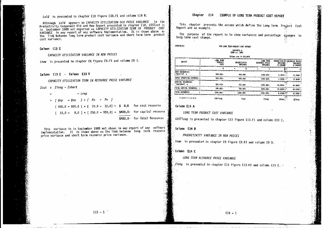
Cha!ter E14 EXAMPLE OF LONG TERN PRODUCT COST REPORT
This chapter presents the axioms which define the Long Term Prqjuct CostReport and an example.
The purpose of the report is to show variances and percentage inlong term cost change.
PROSOCTI VIII RE50JRCE PRICE RARIANCt VARIANCERARIARCE VARIANCE V V CHANGE
COST RESOVRCES:Naterlal a 540.000— 660.000 1100.000— 10.0000
TOTAl OPERA1560 EXPENSES 540.000- 660.000 1200.005— 5.2632:. 50.0050
CAPEIALRES mmcEquipment a soo.ooo— 700.000 1200.000— 20.0000 - 40.0000
Column E14 C
LONG TERM RESOURCE PRICE VARIANCE
?long is presentcd in chapter £13 figure E13.F1 and column £13 E. -
r
1006/09/01 PPN LONG TERN PRCCUCI COST AEPHAT
NOSINESS A1900 vs. 1909
- Values are I, 20L1065
ENTITI1010 TERN
PROS XC I
COST
Lold is presented in chapter £18 figure E18.F1 and column £18 B.
Although Lo7d appears as CAPACITY UTILIZATION OLO PRICE VARIANCE in the
Productivity Component Old and Mew Report presented in chapter E18, COSTcut is
in September 1988 not reported as CAPACITY UTILIZATION TERM IN PRODUCT COST
VARIANCE in any report of any software implementation. It is shown above as
the link between long term product cost variance and short term term product
cost variance.
Column E13 I
CAPACITY UTILIZATION VARIANCE IN NEW PRICES
Lnew is presented in chapter £9 figure E9.F3 and column
E Column E13 H -
CAPACITY UTILIZATION TERM IN RESOURCE PRICE VARIANCE
Zcut m Ziong — Zshort
= —Lrep
= (Qnp —Qne j*( Po — Rn]
600,0 — 600,0 3 * [ 20,0 — 22,0] $ 0,0 for cost resource
12,0 — 8,0] * [ 250,0 — 350,0] = $400,O- for capital resource
$400,O- for Total Resources
This variance is in September 1988 not shown in any report of any software
implementation. It is shown above as the link between long term resource
price variance and short term resource price variance.
£13 — 5 -
FANC 11090
Column E14 A
COOTiveg I've flung 07lsng
LONG TERN PRODUCT COST VARIANCE
COST/ong is presented in chapter £13 figure E13.F1 and column £13 C.
Column E14 B
PRODUCTIVITY VARIANCE IN NEW PRICES
Ynew is presented in chapter £9 figure E9.F1 and column £9 D.
£14 — I
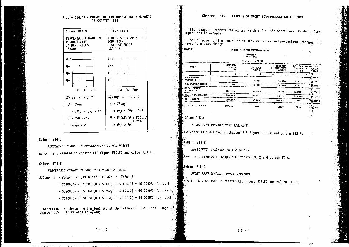
Column EM D Column E14 E
PERCENTAGE CHANGEPRODUCTIVITYIN NEW PRICESA7new
IN PERCENTAGE CHANGE INLONG TERNRESOURCE PRICEA7long
Po Pn Pnr Po Pn Pnr
A?new a A/B a -C /0A = Ynew C = Ziong
mTQnp_QnJ* Pn aqnp*[Po —PnJ
B = VALUEnew
mqn*Pn
0 = VALUEo7d
eQnp*Po
+ VOLold+ Yold
Column E14 D
PERCENTAGE CHANGE IN PRODUCTIVITY IN NEW PRICES
AVnew is presented in chapter E1O figure E1O.Fl and column ElO 0.
Column E14 E
PERCENTAGE CHANGE IN LONG TERM RESOURCE PRICE
Lt7long a — Ziong / [VALUEoId + VOLold + Yold ]
— 51200,0— / [58000,0 + 53400,0 + $ 600,0] = 10,0000% for cost
— $1200,0— / [5 2000,0 + $ 500,0 + $ 500,0] = 40,0000% for capital
— $2400,0— / [510000,0 + 53900,0 + 51100,0] = 16,0000% for Total
Attention is drawn to the footnote at the bottom of the final page
chapter E15. It/relates to IQiong.
umn E15 A
SHORT TERM PRODUCT COST VARIANCE
Tshort is presented in chapter E13 figure E13.F2 and column E13 F.
olumn ElS B
EFFICIENCY VARIANCE IN NEW PRICES
is presented in chapter E9 figure E9.F2 and column E9 0.
olumn E15 C
SHORT TERN RESOURCE PRICE VARIANCE
'short is presented in chapter E13 figure E13.F2 and column E13 H.
Figure E14.F1 - CHANGE IN PERFORMANCE INDEX NUMBERSIN CHAPTER E14
E1S EXAMPLE OF SHORT TERN PRODUCT COST REPORT
This chapter presents the axioms which define the Short Term Product CostReport and an example.
The purpose of the report is to show variances and percentage inshort term cost change.
PPM sHmT TERN CasT PERFOSVGAAICE REP%T
NOsINEss A5968 vs.
are lv ScuMs
ENTITYsVmT TERM
PR HAG C T
COST
58681 TERMEFFICIENCY REIeIRCE PRICE
VARIANCE VARIANCE
EFFICIENCY PRICEVARIANCE 44ARIANCE% CHANGE CHANGE
I 549.000— 660.000 1100.001— 5.2630
62 SHOES 540.000— 660.000 1200.OOO— .2631
1500.000— 700.000— 800.000— 10.0000— - 4P.OOOO
1500.000 10.0000 fl??.
FUNCTIONS COSTslisrE E,ew Eshurt Atvew
E14 — 2 ElS — 1
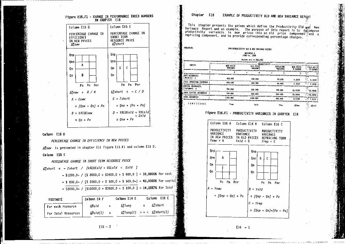
Column E15 D Column E15 E
PERCENTAGE CHANGE
EFFICIENCYIN NEW PRICES
IN PERCENTAGE CHANGE INSHORT TERMRESOURCE PRICEts2short
Po Pn Pnr Po Pn Pnr
a!new a A/B A7short a — C/U
A = Enew C = Zshort
a/Qne_Qnj* Pn aqne*(Po —Pn]
B = VALUEnew 0 = VALUEo!d + VOLold
eQn*Pn aqne*Po+ Eold
Column E15 0
PERCENTAGE CHANGE IN EFFICIENCY IN NEW PRICES
Isrnew is presented in chapter Eli figure Eil.Fl and column Eli D.
Column E15 E
PERCENTAGE CHANGE IN SHORT TERN RESOURCE PRICE
â7short a — Zshort / (VALUE07d + VOLold + Eold .1
— $1200,O— / [$ 8000,0 + $3400,O + $ 600,0] = 10,0000% for cost
{$ 2000,0 + $ 500,O + $ 500,0—] = 40,0000% for capit..
{$i0000,0 + $3900,0 + $ 100,0 ] = 14,2857% for Total
— $ 800,0— /
— $2000,0— /
Figure E15.F1 - CHANGE IN PERFORMANCE INDEX NUMBERSIN CHAPTER E15
Chapter E16 EXAMPLE OF PRODuCTIVITY OLD AND NEW VARIANCE
This chapter presents the axioms which define the Productivity Old qggl NewVariance Report and an example. The purpose of this report is to diEomposeproductivity variances in new prices into an old price component- arepricing component, and to provide corresponding percentage changes.
PPM PROUUCII VIII OLD & REV VARIANCE IEPCRT
905INESD A1908 us. 1989
Values are I, DOLLARS
ENTITY REV PRICEVARIANCE
::::::: ::__:OLD PRICE REPRICING REV PRICE
- PRICEVARIANCE VARIANCE 0 CHARGE - S CHANCE
I
- I
N60.101 601.011 60.008 5.1631 9.2632660.008
700.800
600.008
500.000
60.000
200.000
5.2632
20.0000
--: 0.2632I
20.0000NL CAPITAL RESOURCES
I 700.080 500.000 200.000 20.0000 '20.0000
FORE 2 IONS AsiA Vrep AVuew . A7s1d
Ftgure E16.F1 - PRODUCTIVITY VARIANCES IN CHAPTER E16
Column Ei6 A Column E16 B Column E16 C
PRD0UCTIVITY PRODUCTIVITY PRODUCTIVITYVARIANCE VARIANCE VARIANCEIN NEW PRICES IN OLD PRICES REPRICING TERM
FOOTNOTE Column E4 F
[For each resource
For Total Resources isPold(I)
E15 — 2
Column E14 E Column E15 E
a bjlong a b2short -:
a L2long(I) > = c ts7short(I)
Po Pn Pnr Po Pn Pnr
A=Ynew B=Yold
a[Qnp—Qn]*pn a[Qnp—Qn]*po
C = Yrep
a (Qnp — QnJ*(Pn — PoJ
E16 — 1
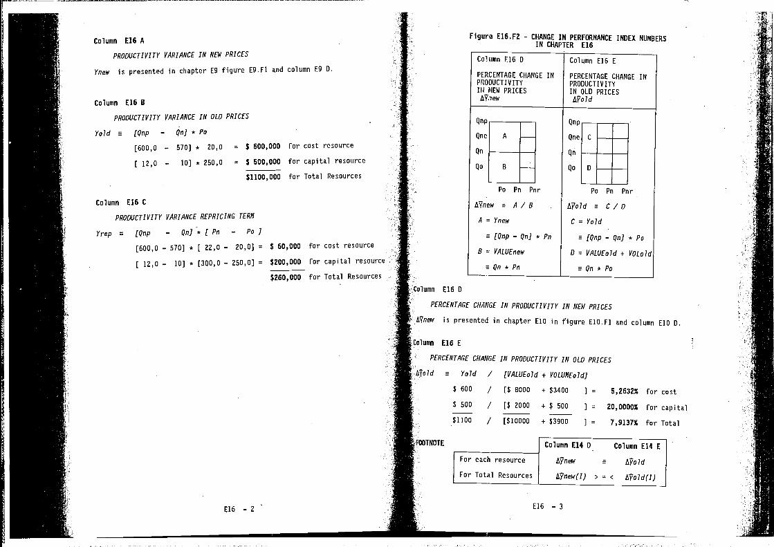
Column E16 A
PRODUCTIVITY VARIANCE IN NEW PRICES
Ynew is presented in chapter E9 figure E9.F1 and column E9 D.
Column E16 B
PRODUCTIVITY VARIANCE IN OLD PRICES
Yold a (Qnp — QnJ * P0
[600,0 — 570] * 20,0
12,0 — 10] * 250,0
Column E16 C
PRODUCTIVITY VARIANCE REPRICING TERM
Yrep a [Qnp — QnJ * I Pn — Po J
[600,0—570] * [ 22,0 — 20,0] = $60,000 for cost resource
12,0 — 101 * [300,0 — 250,0] = $200,000 for capital resource
$260,000 for Total Resources
E16 U
PERCENTAGE CHiINGE IN PRODUCTIVITY
AYnew is presented in chapter ElO in
umn E16
PERCENTAGE CHANGE
old a Yold
$ 600
$ 500
$1100
/ [V/1LUEo1d + VOLUMEoJd]
/ [$ 8000 + $3400
/ [$2000 +$500
/ [$10000 + $3900
Column E14 D Column E14 El
a
> = < AYold(I)
E16 — 3
Figure E16.F2 - CHANGE IN PERFORMANCE INDEX NUMBERSIN CHAPTER E16
= $ 600,000 for cost resource
= $ 500,000 for capital resource
$1100,000 for Total Resources
Column E16 D
PERCENTAGE CHANGEPRODUCTIVITYIn NEW PRICES
IN
Column E16 E
PERCENTAGE CHANGE INPRODUCTIVITYIN OLD PRICES
Qnp
Qne A
Qnp
Qn
Qne C
Qo B
Qn
Qo D
Po Pn
AVnew a A / B
Po Pn Pnr
A=)'new
. AVoid a C / D
a [Qnp — QnJ * Pn
C=Yold
B VALUEnew
a (Qnp — QnJ * Po
aQn*PnD = VALUEo/d + VOLoJd
E
IN NEW PRICES
figure E10.F1 and column ElO 0.
IN PRODUCTIVITY IN OLD PRICES
= 5,2632% for cost
= 20,0000% for capitai
= 7,9137% for Total
E16 — 2
For each resource
For Total Resources
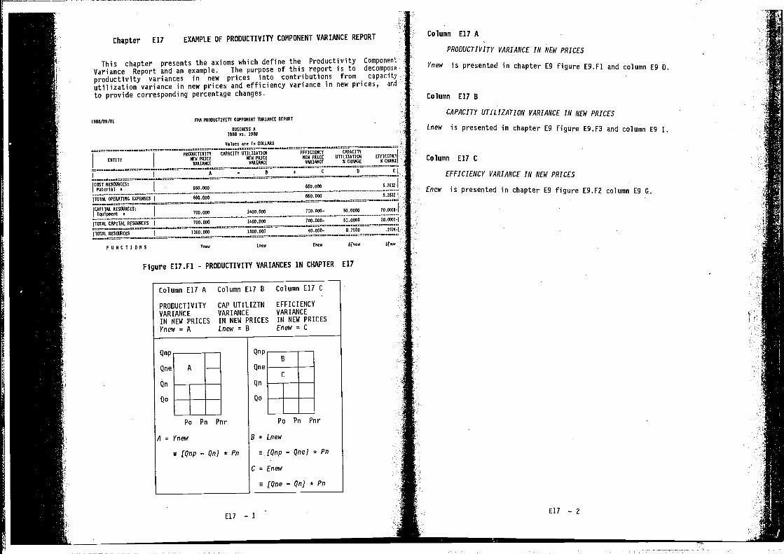
Chapter E17
This chapter presents the axioms which define the Productivity Component
Variance Report and an example. The purpose of this report is to decompose
productivity variances in new prices into contributions from capacityutilization variance in new prices and efficiency variance in new prices, and
to provide corresponding percentage changes.
ENTITY
PPCGOUCTIVIU CAPACITY OTILIZAOION EYIICIENCY CAPACITY
NEW NEW PRICE NEW PRICO UTILIZATION
VARIANCE YAeIANCE VAVIANCE S CHANGE
I
A I + C 0 1
CosT eEsoJeCEs:MateriAl a - 650.000 660.000 5.2632
TeTA. APEP.AIING EXPENSEs o&o.onn 600.003
CAPITAL REsOURCES:Equipment a 100.000 1400.000 100.000— 00.0000 20.0000-
110161 CAPiTAL eEsIoIecEs lnn.eno 1400.000 100.000- 50.0000
ITOIAL stoweCEs 1360.000 1400.000 40.000— 6.7500
Figure E17.FI - PRODUCTIVITY VARIANCES IN CHAPTER E17
Eli — 1E17 — 2
EXAMPLE OF PRODUCTIVITY COMPONENT VARIANCE REPORT
1980/09101 PPM PRONOCTI VITO VARIANCE REPONT
ROSINESS A1906 vs. 1909
Values are in 0011805
Column E17 A
PRODUCTIVITY VARIANCE IN NEW PRICES
Ynew is presented in chapter E9 figure E9.F1 and column E9 D.
Column E17 B
CAPACITY UTILIZATION VARIANCE IN NEW PRICES
Lnew is presented in chapter E9 figure E9.F3 and column E9 I.
Column E17 C
EFFICIENCY VARIANCE IN NEW PRICES
Enew is presented in chapter E9 figure E9.F2 column E9 C.
Column Eli A Column Eli B Column Eli C
PRODUCTIVITY CAP UTILIZTN EFFICIENCY
VARIANCE VARIANCE VARIANCE
IN NEW PRICES IN NEW PRICES IN NEW PRICESYnew=A Lnew=B Enew=C
Po Pn Pnr
A=Ynew
a (Qnp—QnJ*Pn
Po Pn Pnr
B=Lnew
a (Qnp—QneJ *Pn
C = Enew
a (Qne — QnJ *
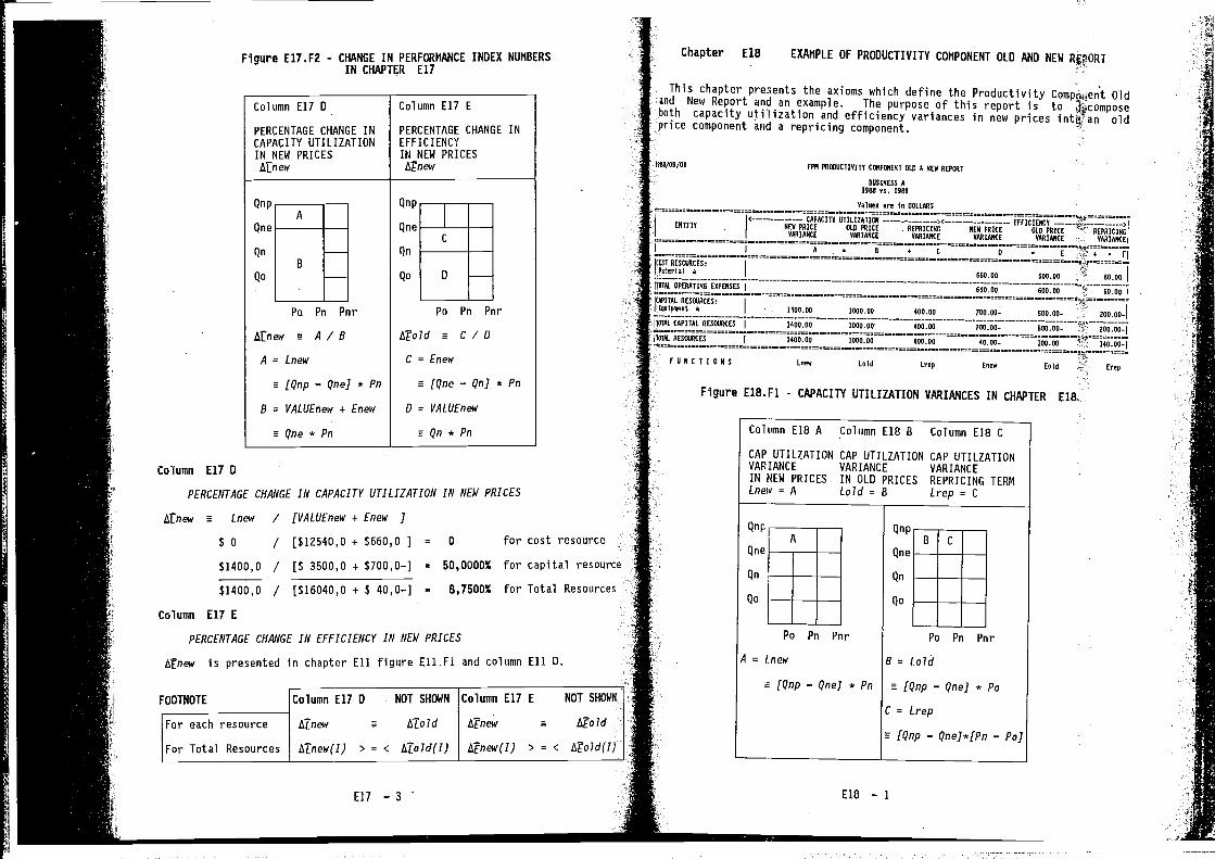
FPN PRmIUCTIVIIV CeIPO4ENT OLD & NEW REPORT
BUSINESS A1988 as. 1989
Values are In IOLLAWI
CAPACITY UTILIZATION —:EFFICIENCYENTITY NEW PUICE OLD PRICE REPRICING NEW PRICE OLD POUCE OEPVICING
YARIUNCE VARIANCE VURIARCE VARIANCE VARIANCE VARIARCE
B + C U
Figure E18.Fl - CAPACITY UTILIZATION VARIANCES IN CHAPTER E18
Column El8 A Column EI8 B Column E18 C
CAP UTILZATION CAP UTILZATION CAP UTILZATIONVARIANCE VARIANCE VARIANCEIN NEW PRICES IN OLD PRICES REPRICING TERMLnmw=A Lold=B Lrep=C
E18 — I
Figure E17.F2 - CHANGE IN PERFORMANCE INDEX NUMBERSIN CHAPTER E17
Chapter Ei8 EXAMPLE OF PRODUCTIVITY COMPONENT OLD AND NEW
Qnp
Qne
Qn
Qo
This chapter presents the axioms which define the Productivity Oldand New Report and an example. The purpose of this report is tobeth capacity utilization and efficiency variances in new prices oldprice component and a repricing component.
Column E17 D
PERCENTAGE CHANGE INCAPACITY UTILIZATIONIN NEW PRICESttnew
Column E17 E
PERCENTAGE CHANGE INEFFICIENCYIN NEW PRICESATnew
Po Pn Pnr
Atnew e A/BA=Lnew
efl7np—QneJ*Pn
B = VALUEnew + Enew
eQne*Pn
Po Pn Pnr
ATold C/DC=Enew
s[Qne—QnJ*Pn
0 = VALUEnew
eqn*Pn
A
:0
- E + F'
FVNCTIUNS
601.01 600.00 : 61.10
661.11 610.11 60.11
1411.11 1000.00 400.01 711.11— - 516.11— —
1411.11 1111.19 401.11 760.00— 500.00—--- 1400:00 400:00 100.00
Lnew bid brep Enew Eoid Erep
Column E17 D
PERCENTAGE CHANGE IN CAPACITY UTILIZATION IN NEW PRICES
Atnew a Lnew / (VALUEnew + Enew j$ 0 / [$12540,O + $660,O = 0 for cost resource
$1400,O / [$ 3500,0 + $700,O—] = 50,0000% for capital resource
$1400,O / [$16040,O + $ 40,0—] = 8,7500% for Total Resources
Column E17 E
PERCENTAGE CHANGE IN EFFICIENCY IN NEW PRICES
aTnew is presented in chapter Eli figure Eil.Fl and column Eli D.
FOOTNOTE Column E17
ATnew
0
a
NOT SHOWN
AEold
Column E17
L?new
E
eFor each resource
For Total Resources Ainew(I) > = c ATold(I) A?new(I) > =
NOT
ATold
< Is?old(I)
A = Lnew
(Qnp — Qne] * Pn
Eli — 3
Po Pn Pnr Po Pn Pnr
B = LoIS
(Qnp — Qne] * Po
C = Lrep
(Qnp — Qne]*(Pn —
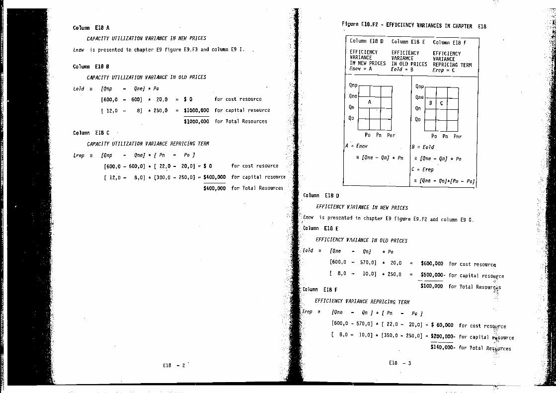
Column E18 B
CAPACITY UTILIZATION VARIANCE IN OLD PRICES
Lold a (Qnp — QneJ * P0
[600,0 — 600] * 20,0
12,0 — 8] * 250,0
Column E18 C
CAPACITY UTILIZATION VARIANCE REPRICING TERM
Lrep a (Qnp — QneJ * I Pn — Pa I
[600,0 — 600,0] * [ 22,0 — 20,0] = $0 for cost resource
12,0 — 8,0] * [300,0 — 250,0] = $400,000 for capital resource
$400,000 for Total ResourcesColumn E18 D
EFFICIENCY ViRIANCE IN NEW PRICES
Enew is presented in chapter E9 figure E9.F2 and column E9 G.
EFFICIENCY IN OLD PRICES
a [Qne — Qn] *Po
[600,0 -. 570,0] * 20,0
8,0 •- 10,0] * 250,0
Iolumn E18 F
EFFICIENCY VARIANCE REPRICING TERM
a [Qne — Qn 3 * [ — Pa 3
[600,0 — 570,0] * [ 22,0 — 20,0] = $ 60,000 for cost resource
1 8,0 — 10,0] * [350,0 — 250,0] = $200,000- for capital
$140,000- for Total
E18 — 3
Column E18 A
CAPACITY UTILIZATION VARIANCE IN NEW PRICES
Lnew is presented in chapter E9 figure E9.F3 and column E9 I.
Figure E18.F2 - EFFICIENCY VARIANCES IN CHAPTER FiB
= $0= $1000,000
$ 1000,000
Column E18 D Column E18 E Column E18 F
EFFICIENCY EFFICIENCY EFFICIENCYVARIANCE VARIANCE VARIANCEIN NEW PRICES IN OLD PRICES REPRICING TERMEnew = A Eold = B Erep C
for cost resource
for capital resource
for Total Resources
Pa Pn Pnr Po Pn Pnr
A=Enew B=Eold
a [Qne — Qn] * Pn a [Qne — Qn] * Po
C = Erep
a [Qne — Qn]*[Pn — Po]
Eo id
= $600,000 for cost resource
= $500,000- for capital resource
$100,000 for Total Resources
E18 — 2
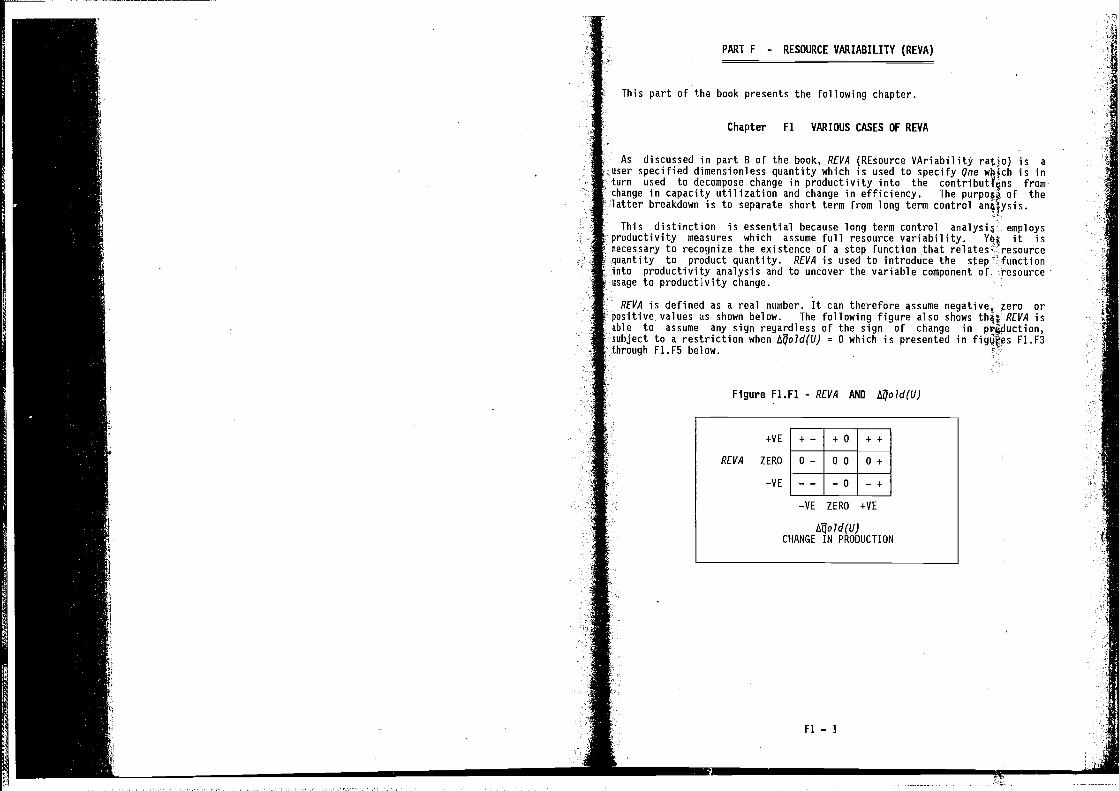
PART F - RESOURCE VARIABILITY (REVA)
This distinction is essential because long term control analysis employsproductivity measures which assume full resource variability. it isnecessary to recognize the existence of a step function that''ntity to product quantity. REV/i is used to introduce the step function
productivity analysis and to uncover the variable component of. resourceto productivity change.
REV/i is defined as a real number. It can therefore assume zero orositive. values shown below. The following figure also shows that REVA isble to assume any sign regardless of the sign of change in
to a restriction when = 0 which is presented in F1.F3through F1.F5 below.
Figure F1.FI - REV/i AND
Fl — 1
This part of the book presents the following chapter.
Chapter Fl VARIOUS CASES OF REVA
As discussed in part B of the book, REV/i (REsource VAriability ratio) is a
specified dimensionless quantity which is used to specify Qne is inturn used to decompose change in productivity into the from-change in capacity utilization and change in efficiency. The of thelatter breakdown is to separate short term from long term control
+VE +— -i-0 ++
REVA ZERO 0— 00 0+
—yE —— —O —+
—yE ZERO +VE
ld(U)CHANGE IN PRODUCTION
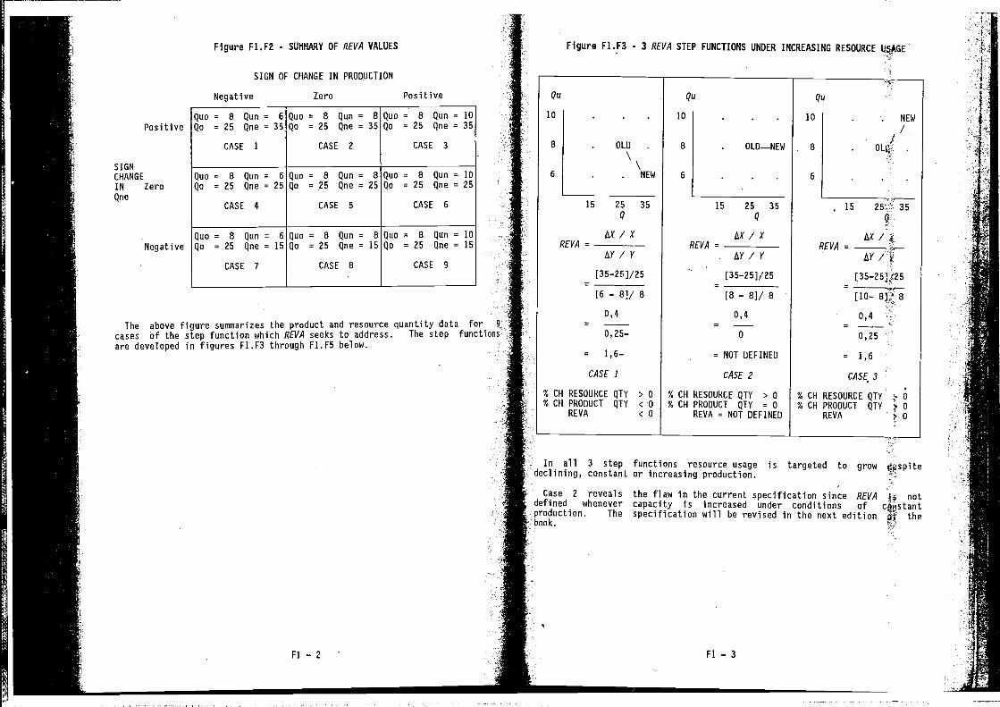
Figure F1.F2 - SUMMARY OF REVA VALUES
— [35—251/25
[6 — 8]/8
0,4
0,25—
1,6—
CASE I
RESOURCE QTY > 0PRODUCT QTY < •0REVA <0
@1
10
8
6
15 25 35Q
REVA =
__________
LY/Y
— [35—251/25
- [8 - 8J/ 8
Qu
10 . NEW
/8 .
6
15 35
Q
RE VA =lxY /
—
[10— 811 8
0,4
0,25
= 1,6
CASE 3
% CH RESOURCE QTY% CH PRODUCT QTY
REVA
Negative
SIGN OF CHANGE IN PRODUCTION
Zero Positive
SIGNCHANGE
INQne
Positive
Zero
Negative
Figure F1.F3 - 3 REVA STEP FUNCTIONS UNDER INCREASING RESOURCE USAGE
Quo = 8 Qun = 6
Qo = 25 Qne = 35
CASE 1
Quo = 8 Qun = 8
Qo = 25 Qne = 35
CASE 2
Quo = 8 Qun = 10Qo = 25 Qne = 35
CASE 3
Quo = 8 Qun = 6
Qo = 25 Qne = 25
CASE 4
Quo = 8 Qun = 8
Qo = 25 Qne = 25
CASE 5
Quo = 8 Qun = 10Qo = 25 Qne = 25
CASE 6
Quo = 8 Qun = 6
Qo = 25 Qne = 15
CASE 7
Quo = 8 Qun = B
Qo = 25 Qne = 15
CASE 8
Quo = 8 Qun = 10Qo = 25 Qne 15
CASE 9
Qu
10
8 OLD
\\
6 NEW
15 25 35Q
REVA= —/ Y
OLD—NEW
% CH% CH
0,4
0
= NOT DEFINED
CASE 2
% CH RESOURCE QTY > 0% CH PRODUCT QTY = 0
REVA = NOT DEFINED
The above figure summarizes the product and resource quantity data for 9
cases of the step function which REVA seeks to address. The step functionsare developed in figures F1.F3 through F1.F5 below.
Fl — 2
In all 3 step functions resource usage is targeted to growdeclining, constant or increasing production.
Case 2 revealsdefined wheneverproduction. Thebook.
the flaw in the current specification since REVA notcapacity is increased under conditions ofspecification will be revised in the next edition the
Fl — 3
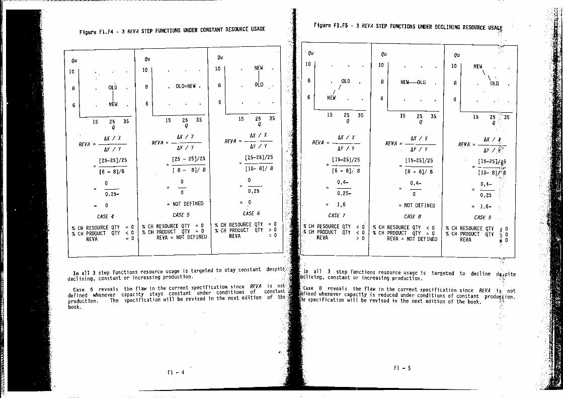
25
Q
AX/XREVA
/ V
In all 3 step functions resource usage is targeted to stay constant despite
declining, constant or increasing production.
Case 5 reveals the flaw in the current specification since REVA is
defined whenever capacity stays constant under conditions of constant
production. The specification will be revised in the next edition of the
book.
Fl — 4
In all 3 step functions resource usage is targeted to declineining, constant or increasing production.
8 reveals the flaw in the current specification since REVA notrifled whenever capacity is reduced under conditions of constant
specification will be revised in the next edition of the book.
Fl — 5
Figure F1.F4 - 3 REVA STEP FUNCTIONS UNDER CONSTANT RESOURCE USAGE
Qu Qu
10 . .. 10
8
6
Qu
10
OLD
NEW
Figure F1.F5 - 3 REVA STEP FUNCTIONS UNDER DECLINING
Qu
10
15
RESOURCE USAGE
8 OLD
//
NEW6
8 . OLD=NEW
6
35 15 25
Q
AX/XREVA =
AY / V
— [25 — 251/25
[8-. 81/80
0
NOT DEFINED
CASE 5
% CU RESOURCE QTY = 0% CH PRODUCT QTY = 0
REVA = NOT DEFINED
25 35Q
NEW
8 . OLD
6
15 25 35
Q
M/XREVA =
AY / V
[25—25]/25
- [10— 8J/ 8
0
0,25
=0CASE 6
% CU RESOURCE QTY = 0% CH PRODUCT QTY > 0
REVA =0
— [25—25]/25
— [6 — 81/8
0
0,25—
= 0
CASE 4
% CH RESOURCE QTY = 0% CU PRODUCT QTY < 0
REVA =0
Qu
10
8 NEW—OLD
6
15 25 35Q
AX/XREVA =
__________
LIV/Y
— [15—251/25
- [8 - 8]/ 8
0,4—
0
= NOT DEFINED
CASE 8
% CH RESOURCE QTY < 0% Cl-I PRODUCT QTY = 0
REVA = NOT DEFINED
15
REVA -—/ V
— [15—25]/25
[6 — 8
0,4—
0,25—
= 1,6
CASE 7
CU RESOURCE QTY < 0CH PRODUCT QTY < 0
REVA >0
Qu
10 NEW
\ \-8 . OLD
6
15
REVA =
_______
—
[10- 8)73
0,4—
— 0,25
= 1,6—
CASE 9
% CU RESOURCE QTY 0% CH PRODUCT QTY 0
REVA
PART G — PROXY DATA
This part of the book presents the following 2 chapters.
Chapter GI PROXY PRICES AND QUANTITIES WHEN NONE ARE AVAILABLE
Chapter G2 SCORING MATRICES FOR PROXY PRODUCT QUANTITY
Chapter Gl PROXY PRICES AND QUANTITIES WHEN. NONE ARE
Proxy prices for product and resources
The value axiom is the fundamental identity on which this work rests, Sincevalue is defined as the product of quantity and pricw, it is simplyto find two of the three functions and the model will derive thirdfunction. Although the data to populate the model exist, they are ofteninaccessible on grounds of cost of capture.
Readers would then be advised to use the value data, which areavailable, and to resort to price proxies for product and variabledata and to quantity proxies for fixed resources. Public priceproxies are provided by the price series published by government
a monthly basis. Use of published statistical wouldrequire the reader to assign individual series to specific product ähd costentities. Fixed capital proxies are normally easy to make if one a
a base period and then enquires from mapgementwhat is the relative capacity in a later period.
Proxy product quantities
If the accounting system allocates resources but not products to givencost center, it is necessary to define "proxy products" formeasurement and control. A familiar illustration is the shared resot*Ie caseof common costs categories. For example, corporate resources which fle notattributed to the individual businesses which carry their own costswould fall into this category.
When an operation contains no specified product, the model requires that theuser indicate which, of the set of operations that do have productsmust be used for proxy products in that particular operation.
Scalars for proxy product and resource quantities
Another need for oroxy data involving the use of scalars arises inapplications which compare operations in which technologies, aredissimilar in process or in order of scale, make identical Forexample, an electrical engineer enrolled for an MSc degree usingdeterministic productivity accounting to compare two different powertechnologies which make a homogeneous electricity of the same persecond. Similar research is being conducted by a mining engineer; alsoenrolled for an MSc degree, to compare two different mining technologii4 whichmake identical product. A simpler need for scalars arises incomparisons to avoid the analysis being swamped by a spuriousutilization effect caused by a spurious REVA.
G1 — I
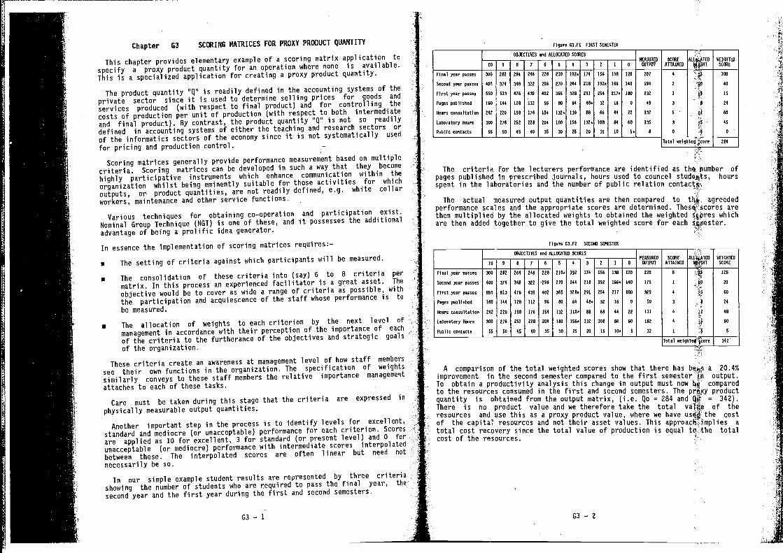
This chapter provides elementary example of a scoring matrix application to
specify a proxy product quantity for an operation where none is available.This is a specialized application for creating a proxy product quantity.
The product quantity "Q" is readily defined in the accounting systems of theprivate sector since it is used to determine selling prices for goods and
services produced (with respect to final product) and for controlling the
costs of production per unit of production (with respect to both intermediate
and final product). By contrast, the product quantity "Q" is not so readilydefined in accounting systems of either the teaching and research sectors or
of the informatics sectors of the economy since it is not systematically used
for pricing and production control. —
Scoring matrices generally provide performance measurement based on multiple
criteria. Scoring matrices can be developed in such a way that they become
highly participative instruments which enhance communication within the
organization whilst being eminently suitable for those activities for which
outputs, or product quantities, are not readily defined, e.g. white collarworkers, maintenance and other service functions.
Various techniques for obtaining co—operation and participation exist.Nominal Group Technique (NGT) is one of these, and it possesses the additionaladvantage of being a prolific idea generator.
In essence the implementation of scoring matrices requires:—
• The setting of criteria against which participants will be measured.
• The consolidation of these criteria into (say) 6 to 8 criteria per
matrix. In this process an experienced facilitator is a great asset. The
objective would be to cover as wide a range of criteria as possible, withthe participation and acquiescence of the staff whose performance is to
be measured.
• The allocation of weights to each criterion by the next level of
management in accordance with their perception of the importance of each
of the criteria to the furtherance of the objectives and strategic goals
of the organization.
These criteria create an awareness at management level of how staff members
see their own functions in the organization. The specification of weights
similarly conveys to these staff members the relative importance management
attaches to each of these tasks.
Care must be taken during this stage that the criteria are expressed in
physically measurable output quantities.
Another important step in the process is to identify levels for excellent,
standard and mediocre (or unacceptable) performance for each critorion. Scoresare applied as 10 for excellent, 3 for standard (or present level) and 0 for
unacceptable (or mediocre) performance with intermediate scores interpolated
between these. The interpolated scores are often linear but need not
necessarily be so.
In our simple example student results are represented by three criteriashowing the number of students who are required to pass the final year, the
second year and the first year during the first and second semesters.
G3 — 1
OBJECTIVES and AlLOCATED SCORESMEASURED SCORE
ATRAIHED
4
2
ALLOCATED WEIGHTED
SCORE
100
40
Final year passes
Sec,,d year passes
—10
30A
404
—9
292
374
—H
264
349
—7
246
322
—6
228
296
—5
210
270
—4
192a
244
—3
174
218
—2
156
IH2a
—I
13W
166
—0
128
14W
tIITPUT
287
194
First year passes 550 513 476 439 402 365 328 291 254 217* 184 232 1 15
PaRes published 160 144 126 lID 96 86 64 48a 32 16 H 49 3 8 24
Assrs censuitatiss 247 220 196 178 114 132* 11W 66 66 44 22 137 5 0 HO
Lubsratsry Hears 300 276 252 220 204 180 156 132a 108 84 HH 135 3 45
PubliccentacE, 55 00 45 40 35 30 25 20 15 10 Ha H 0 9 •
Tetal eeigete4 284
The criteria for the lecturers performance are identified as the pumber ofpages published in prescribed journals, hours used to councel studafls, hoursspent in the laboratories and the number of public relation contactj.
The actual measured output quantities are then compared to thi agreededperformance scales and the appropri4te scores are determined. arethen multiplied by the allocated weights to obtained the weighted sflres whichare then added together to give the total weighted score for each
Finalyearpannen
OBJECTIVES and ALLOCATED SCCAES— — — — — — — — — — — HEASUHEO
EtITFUT
220
SCORE
ATTAINED
5
WIGHTWEIGHTED
SCORE
US
16
300
9
U?
6
U4
7
246
6
228
5
flDa
4 3
lU
2
166
1
138
H
120
Secnnd year passe,
First year passe,
Page, published
Huur,c,n,ulEaEi,e
Laberatery Hears
Public cuntactn
420
594
160
242
300
55
374
513
144
220
276
DV
348
476
128
198
152
45
322
439
212
176
216
40
'296
402
96
154
1V4
35
270
385
80
132
186
30
244
329*
64
110*
166*
25
218
291
48*
88
132
20
192
254
32
66
108
IS
166*
217
16
64
84
IHa
140
IWO
0
20
6W
5
175
329
50
111
162
12
1
4
3
4
4
1
uA
Al
5
22
60
24
48
HO
5
A comparison of the total weighted scores show that there has a 20.4%Improvement in the second semester compared to the first semester in output.To obtain a productivity analysis this change in output must now comparedto the resources consumed in the first and second semesters. The productquantity is obtained from the output matrix, (i.e. Qo = 284 and = 342).There is no product value and we therefore take the total value of theresources and use this as a proxy product value, where we have the costof the capital resourcos and not their asset values. This a
total cost recovery since the total value of production is equal the totalcost of the resources.
Chapter G3 SCORING MATRICES FOR PROXY PRODUCT QUANTITY Figure 63.F1 FIHST SEHESTE6
Figure 03.F2 SECOND SEHESOEH
lutal weighte4icere 342
L
G3 — 2
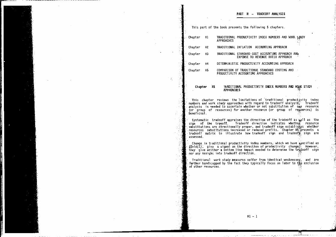
4
PART H — TRADEOFF ANALYSIS
This part of the book presents the following 5 chapters.
Chapter HI TRADITIONAL PRODUCTIVITY INDEX NUMBERS AND WORKAPPROACHES
Chapter H2 TRADITIONAL INFLATION ACCOUNTING APPROACH
Chapter H3 TRADITIONAL STANDARD COST ACCOUNTING APPROACH ANIiEXPENSE TO REVENUE RATIO APPROACH
Chapter H4 DETERMINISTIC PRODUCTIVITY ACCOUNTING APPROACH
Chapter H5 COMPARISON OF TRADITIONAL STANDARD COSTING ANDPRODUCTIVITY ACCOUNTING APPROACHES
Chapter Hi TRADITIONAL PRODUCTIVITY INDEX NUMBERS AND WONK STUDYAPPROACHES
This chapter reviews the limitations of traditional productivity indexnumbers and work study approaches with regard to tradeoff analysH Tradeoffanalysis is needed to ascertain whether or not substitution of o*e resource
• (or group of resources) for another resource (or group of reflurces) isbeneficial.
Systematic tradeoff appraises the direction of the tradeoff as Wi11 as thesign of the traeoff. Tradeoff direction indicates whethof resource
• substitutions are directionally proper, and tradeoff sign whetherresources substitutions increased or reduced profits. Chapter a
tradeoff matrix to illustrate how tradeoff sign and tradeoff- sign areassessed.
Change in traditional productivity index numbers, which we have asAVold(I), give a signal on the direction of productivity However,they give neither a bottom line impact needed to determine the trjdeoff signnor any insight into tradeoff direction.
Traditional work study measures suffer from identical weaknessek. and arefurther handicapped by the fact they typically focus on labor to exclusionef other resources.
Hi — I
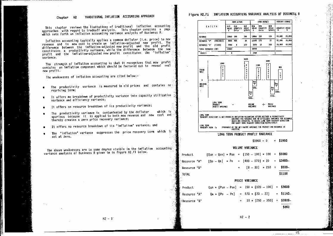
The weaknesses of inflation accounting are cited below:—
• The productivity variance is measured in old prices and contains no
repricing term;
• It offers no breakdown of productivity variance into capacity utilizationvariance and efficiency variance;
• It offers no resource breakdown of its productivity variance;
• The productivity variance is contaminated by the deflator which is
spurious because it is applied to both new revenue and new cost and
thereby creates a zero price recovery variance;
• It offers no resource breakdown of its "inflation" variance; and
i The "inflation" varianco suppresses the price recovery term which is
set at zero.
The above weaknesses are to some degree visible in the inflation accountingvariance analysis of Business B given in in figure H2.F1 below.
ENTITY
REHENOE
OLD OLD OLD
RALOE QOANTITT PRICENEN NEW NEN
OALOE QUANTITY PRICE QUANTITY PRICE
S UnIts 9/1JnIE
11001 III III
$ OnlEs 8/OnIE
10010 150 Ill
S S
50,000 00,000
RESOURCE (VARIABLE) 8000 400 DO 10540 570 00 40,100 10,000
RESOURCE (FISED)
TOTAL RESOURCE COST
PRom
DIII 8 210
10000
3100 II 350
10048
01,000 41.101
0 1908
50083008
1908P 1100 P
I
500—I
J 1140-3400—
LUND TERNPROUOCT = HOLUNE 4-. PRICE
PROFIT VARIANCE VARIANCE VARIANCE
LORO TERNTRADEOFF DIRECTIOU NOT KORAN AS INFLATICNI ACCOUNTINO OFFERS NEITHER A PROUUCTIHITT
VARIANCE PER RESOURCE NOR AN EFFICIENCY RARIANCE PER RESOURCEN4ICN ARE ESSENTIAL TO ASSESS LORD TERN TRASEOFF BIAECTIOUAND SHOUT TERN TRAOEOFF DIRECTION RESPECTIAELY
LOUD TERNTRADEOFF SOON FAVORABLE AS THE NET HOLUNE RARIANCE FOR PNOUACT AND RESOURCE IS
POSITINE
LONG TERM PRODUCT PROFIT VARIANCE
$1960 — 0 = $1960
Chapter H? TRADITIONAL INFLATION ACCOUNTING APPROACH
This chapter reviews the limitations of traditional inflation accounting
approaches with regard to tradeoff analysis. This chapter conatins a page
which sets forth an inflation accounting variance analysis of Business B.
Inflation accounting typically applies a common deflator (i.e. price) to newrevenue and to new cost to create an inflation—adjusted new profit. The
difference between the inflation—adjusted new profit and the old profitconstitutes a productivity variance, while the difference between the nRW
profit and the inflation—adjusted new profit constitutes the "inflation"variance.
The strength of inflation accounting is that it recognizes that new profitcontains an inflation component which should be factored out to reveal real
new profit.
Figure H2.F1 INFLATION ACCOUNTING VARIANCE ANALYSIS OF BUSINESS B
VOLUME VARIANCE
Resource "A" [Qo — Qn] * Po = [400 — 570] * 20 = $3400—
Resource "B" = [8 — 10] * 250 = $500—
TOTAL $1100
Product Qun * [Pun
PRICE
— Puo] =
VARIANCE
150 * [120 — 100] = $3000
Resource "A" Qn * [P0 — Pn] = 570 * [20— 22] = $1140—
Resource "B" = 10 * [250 — 350] = $1000—
H2—Y H2—2
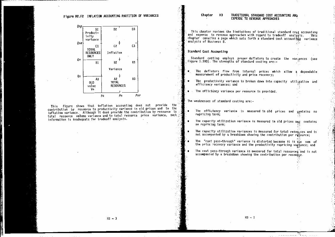
Chapter H3 TRADITIONAL STANDARD COST ACCOUNTING ANUEXPENSE TO REVENUE APPROACHES
This chapter reviews the limitations of traditional standard cost accountingand expense to revenue approaches with regard to tradeoff Thischapter conatins a page which sets forth a standard cost varianceanalysis of Business B.
Standard Cost Accounting
Standard costing employs proper deflators to create the vanances (seeFigure 1.39D). The strengths of standard costing are:--
• The deflators flow from internal prices which allow a dependablemeasurement of productivity and price recovery;
• The productivity variance is broken down into capacity utillntion andefficiency variances; and
• - The efficiency variance per resource is provided.
The weaknesses of standard costing are:—
• The efficiency variance is measured in old prices and norepricing term;
• The capacity utilization variance is measured in old prices containsno repricing term;
• The capacity utilization variances is measured for total and isnot accompanied by a breakdown showing the contribution per
• The "cost pass—through" variance is distorted because it is sum ofthe price :-ecovery variance and the productivity repricing valance; and
• The cost pass—through variance is measured for total resources and is notaccompanied by a breakdown showing the contribution per
Figure H2.F2 INFLATION ACCOUNTING PARTITION OF VARIANCES
QnpDI D2 D3
Product—lvi tyvariance
Qne -I- -Cl C2 C3
TOTALRESOURCES Infl ati on
ONLY
Qn +Bl B2 B3
Van ance
Qo +Al A2 A3
OLD TOTAL
value RESOURCES
Vo
Po Pn Pnr
This figure shows that inflation accounting does not provide the
contribution by resource to productivity variance in old prices and to the
inflation variance. Although it does provide the contribution by resource te
total resource volume variance and to total resource price variance, such
information is inadequate for tradeoff analysis.
H2—3 H3 — I
-4
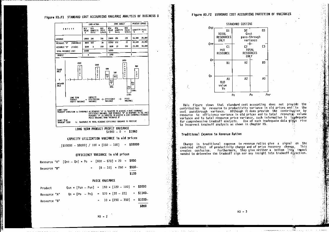
Figure H3.F1 STANDARD COST ACCOUNTING VARIANCE ANALYSIS OF BUSINESS B
ENTITY
1988 ACTUAL 1989
OLD OLD OLD
VALUE QUANTITY PRICE
5 Units 1/Unit
HEN HEN
VALUE QUANTITY PRICE
9 UniEs 5/UnIEQUANTITY PRICE
S S
REVENUE 10008 108 108 18008 ISO 100
570 DO
SD,RO0 10,000
48.50010,000RESOURCE 'U' (VARIABLE)
RESOURCE 'I' (FIXED)
TOTAL RESOURCE COST
OSOR 400 DR
0000 U DOD 3908 ID 3D0 09,000 40,000
10000 IUR4O
PRUFIT 8 1988
3000
600
BUD
500- Hen
1000-
1140-
—4— EFFICIENCY —4—PRICE
RARIANCE VARIANCE
SHOUT TERMTRADEOFF DIRECTION is FAVOURILE AS RESOURCE 'A' IS TARGETED 10 ACHIEVE A MOUE FAVOUABLE
EFFICIENCY RARIANCE THAN RESOURCE 'B' IN RESPONSE TO TUE FACTRESOURCE 'U' IS TARGETED TO ACHIEVE A LESS FAVOUABLE RESOURCE
PRICE VARIANCE TUAR 'RESOURCE B'
SHOUT TERNTRADEOFF SIGH Is FUROUABLE AS TOTAL RESOURCE EFFICIENCY VARIANCE IS POSITIVE
LONG TERM PRODUCT PROFIT VARIANCE$1960 — 0 = $1960
CAPACITY UTILIZATION VARIANCE in old prices
[$10000 — $8000] 100 * [150 — 100] = $10000
EFFICIENCY VARIANCE in old prices
Resource "A" [Qne — Qo] * Po = [600 — 570] * 20 = $600
Resource "B" = [8—10] *250= $500—
$100
Figure H3.F2 STANDARD COST ACCOUNTING PARTITION OF VARIANCES
Qnp
Qne
'5"
Qo
STANDARD COSTING
Po Pn Pnr
This figure shows that standard cost accounting does not provide thecontribution by resource to productivity variance in old prices to thecost passthrough variance. Although it does provide the contribflion by
resource to efficiency variance in old prices and to total resourcø: volumevariance and to total resource price variance, such information isfor comprehensive tradeoff analysis. Use of such inadequate data giVjjs riseto incorrect tradeoff analysis as shown in chapter H5.
Traditional Expense to Revenue Ratios
Change in traditional expense to revenue ratios give a signal on thecombined effect of productivity change and of price recovery changa. Thiscreates confusion. Furthermore, they give neither a bottom impactneeded to determine the tradeoff sign nor any insight into tradeoff direction.
Dl 02 D3
TOTAL CostRESOURCES pass—through
ONLY variance+Cl C2 C3
PER TOTALRESOURCE RESOURCES
ONLY
Bi B2 - B3
Al AZ - A3
OLDvalue
Vo
PRICE VARIANCE
Product Qun * [Pun — Puo] = 150 * [120— 100] = $3000
Resource "A" Qn * [P0 — Pn] = 570 * [20—22] = $1140—
Resource "B" = 10 * [250 — 350] = $1000—
$860
H3-2H3 —
-4
I3
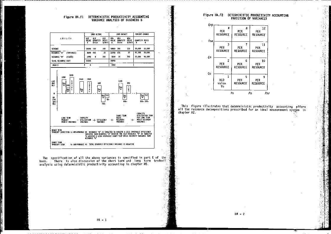
Figure H4.Fl DETERMINISTIC PRODUCTIVITY ACCOUNTINGVARIANCE ANALYSIS OF BUSINESS B
E N I I I Y
1988 ACTUAL 1989 BUDGET PERCENT CVANOE
OLD OLD OLD
VALUE QUANTITY PRICE
$ Units N/Unit
NEW MEW MEW
VALUE QUANTITY PRICE
$ Units S/UnitQUANTITY PRICE
0 0
REVENUE 10000 IDO 100 18000 150 120 50,000 20,000
RESOURCE (VONIABLE)
RESOURCE 9 (FIlED)
IRTAL RESOURCE COST
8000 400 20
2000 8 050
12540 570 22
3500 10 350
42,500 10,000
25,000 40,000
10000 16040
PROFIT 0 1960
19601860
1400 14001200FAN I
660 800OTA Rs
I
0 — — — — 1i___I±i —
—
ON B B
FAR • 40
COO 600— 200— 200—
BLE 700- -
CAPACITYSHOUT TERM UTILIZATION TERN
LONG TERM CAPACITY PRICE FOR LONG IE60IRECOVERY —4-- PRICE RECOVERYPRORUCI = BTILIZAIIOM —4— EFFICIENCY —4—
PROFIT VOUIUNCE VARIANCE VARIANCE VARIANCE VARIANCE
SHOUT TERMTRADEOFF DIRECTION is UNFAVOUABLE AS RESOURCE B IS TARGETED TO ACHIEVE A LESS FANcITABLE EFFICIENCY
VARIANCE 116AM RESOURCE A DESPITE THE FACT RESOURCE B IS TURGETEDTO ACHIEVE A LESS FAVOUARLE SVOUT TERM PRICE RECOVERY VARIANCE 11600RESOURCE A
SHOUT TERMTRADEOFF SIGN Is OMFVVCOARLE AS TOTAL RESOURCE EFFICIENCY VARIANCE IS NEGATIVE
The specification of all the above variances is specified in part E ofbook. There is also discussion of the short term and long termanalysis using deterministic productivity accounting in chapter H5.
Figure H4.F2 DETERMINISTIC PRODUCTIVITY ACCOUNTINGPARTITION OF VARIANCES
17,ie
4PER
RESOURCE
8PER
RESOURCE
12PER
RESOURCE
çn
Qo
3
PER
RESOURCE
7PER
RESOURCE
11PER
RESOURCE
2
PER
RESOURCE
6
PERRESOURCE
10PER
RESOURCE
1
OLD
valueVo
5
PER
RESOURCE
9
PER
RESOURCE
This figure thatall the resource decompositionschapter A2.
'5.,,,
Po Pn Pnr
deterministic productivity accounting offersprescribed for an ideal measurement systom in
H4 — 2
I
H4 — I
k
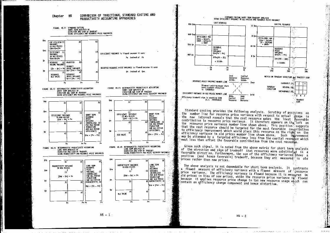
Standard costing provides the following analysis. Scrutiny of onthe number line for resource price variance with respect to actual (jsage inthe new interval reveals that the cost resource makes the least t1avorablecontribution to resource price variance. It therefore appears on onthe resource price variance number line shown above. This position suggeststhat the cost resource should be targeted for the most favorable cohfributionto efftciency improvement which would place this resource on the righj on theefficiency variattce in old prices number line shown above. Suchmay be attended by a targeted efficiency loss from the capital resouEce whichmust less than offset the favorable contribution from the costGiven such signal, it is noted from the above matrix for short terqj analysisof the direction and sign of tradeoff that resources were in afavorable directon. Furthermore, the sum of the efficiency variances shows apositive (and hence favorable) tradeoff, because they are measured in oldprices rather than new prices. -
The above analysis is not dependable for short term analysis. It- flawed measure of efficiency variance with a flawed measure of resourcevariance. The efficiency variance is flawed because it is meaAijred in.J prices in lieu of new prices, while the resource price variance flawedbecause it applies resource price change to the new resource usage which cancontain an efficiency change component and hence distortion.
FIGURE W5.FI STANDARD COSTINGbOUT TERN ANALYSIS SFDIRECTIcN AND SIGN SF TUADEGFFRUING EFFICIENCY AND REIaJRCE PRICE VARIANCES
qep
Qow
Re
Qo
Chapter H5 COMPARISON OF TRADITIONAL STANDARD COSTING ANOPRODUCTIVITY ACCOUNTING APPROACHES
EFFICIENCU VARIANCE Is flawed becaosw It uses
Ps test,ad of Fe
ADJU5IEII RESOURCE PRICE VARIANCE Is flawed becasue YR uses
Qe Iestead of Roe
CAP UTILIZTII UIVARIANCEIN OLD PRICES(Rep—New] Fe
Dl 13
EFFICIENCY CIVARIANCEIN OLD PRICES(Qew-Qo I Fe
CD CI
63
A3
RESCARCE UIVGLUNE VARIANCE
(Re — Re] * Fe
AlRESEeRCERID VALUE
ADJUSTED Dl
PRODUCT
PRICE VARIANCEQuo (Fun — Fus)
AlRES000CEPRICE VARIANCEQe .a (Fe — Fe]
STANDARD EDITING SNOUT TERM TRADEGFF ANALYSISUSING EFFICIENCY VARIANCE IN VII PRICES P341 RESOURCE PRICE VARIANCE
COST RESeIRCE
Fe Fe Per
FIGURE NS.FD DETERMINISTIC AlT? ACCOUNTING
SAOUT TERN ANALYSIS OFDIRECTION AND SIGN OF TRADEOFFUSING EFFICIENCY AND RESOUACE PRICE VARIANCES
FIGARE AS.F3 DETERMINISTIC PR000CTIVITY ACCOUNTINGSNOUT TERN ANALYSIS OFDIUECIION AND SIGN OF IRAGCGFFUSING EFFICIENCY AND PRICE RECOVERY VARIANCES
CssE CapItalResource Resource$1140- $1000-
YEDOURCE PRICE VARIANCE NARUER LINESown
\ /UtaRsuaf patrtng mea,s short \ /,Own tradeoff dtrwctluse /to FAAARAULE / \
EFFICIENCY RARIANCE IN GIl PRICES NANRER LINE" "
Estd1500— SOlDEfflcteecy GradwoFf stge to psstttyw DUOS Cwptcel CesE(I.e. FAAOUAULE) Resource ResourceRep --
Quo
Re
Ye
RepDl
QewCl
SACNT TERNRESOURCE
PRICE
Re VARIANCE(UtOUNUALIOED AlFOU NEA PGRIOUPRODUCTION
AND OlD FERIOU
Rs EFFICIENCY)AS
Row w (Pu — P0)
Fe Fe
FIGURE AN.F4 DETERNINIGTIC PRODUCTIVITY ACCOUNTINGLONG TERN ANALYSIS OFDIRECTION AND SIGN OF 1RADEOFFUSING PRODUCTIVITY AND REGOURCE PRICE YOUIAACEG
Dl' Dl
Cl C3
EFFICIENCY VARIANCE
IN Nflt PRICES(Qew — Re] 5 Fe
Ut II
Al AD
OLD YALGE
SAOUT TERNPRICE
RECOVERY
VARIANCE(VeRNALIZED UT
FOU NEW PERIODPR005CTIONAND OLD PERIODEFFICIENCY)
AS
Roe o (Per — Fe)
NAYNIS ON TRADEOFF DIRECTIOU TRADEOFF SIGN
FAOOUARLE )F(
TRADEOFF NEUTRAL (NbUIRECY)OU
UNFAYOUAILE (tip
IN F
TRADEOFFSIGN
Fe Pc Pu
FIGURE R5.F6 OETERNINISTIC FROUUCTIOITA ACCOUNTINGLONG TERN ANALYSIS OFDIRECTION AND SIGN OF TRADEOFFUSING PRODUCTIVITY AND PRICE RECRAORY VARIANCES
Rep
Quo
Re
Re
Dl' Dl Dl
FROUUCTIAITA VARIANCE LONG TERN
IN NEA PRICES RESOUACE
4 PRICE
CI Cl VARIANCE CD
(NOUNUALIOED
(Rep — Qe] a Fe tOU NEW PERIODFROUSCTIENAND OIl FERIOU
UI ID FROUACIIAITA) Il
Rep a )Ps — Fe]
Al Al - Al
Fe Pope Fe
Rep
Qee
Ye
Ye
TERNPROUACTIVITY VARIANCEIN NEW FRICEG
4Cl
(Rep — To] a Fe
Ut
Cl
ID
PRICERECAYERY
VARIANCE Cl(NOUNALIOESFOU NEW PERIODPRODUCTION
AND RID PERIODFVODUCTIAIIT) Dl
Qep a (For — Fe]
AlOLD VALUE
Al A3
Fe F,
115 — 1 -,
Per
115 — 2
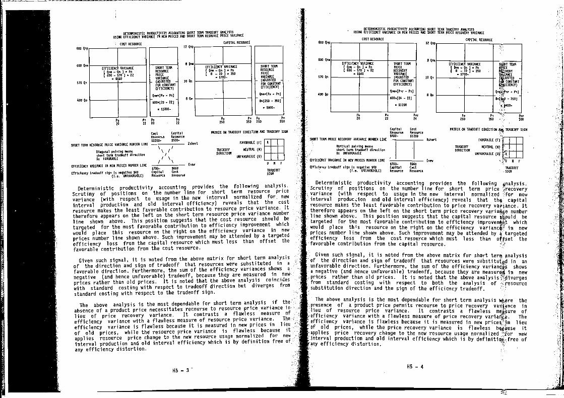
Pu20 22
Cost CapitalResource Resource$1200- $000-
Cohort
\ /
/\/ \
Esew
1700— 0660Capital CostResource Resource
Deterministic productivity accounting provides the following analysis.Scrutiny of positions on the number line for short term resource price
variance (with respect to usage in the new interval normalized for new
interval production and old interval efficiency) reveals that the cost
resource cakes the least favorable contribution to resource prfce variance. Ittherefore appears on the left on the short term resource price variance number
line shown above. This position suggests that the cost resource should be
targeted for the most favorable contribution to efficiency improvement which
would place this resource on the right on the efficiency variance in new
prices number line shown above. Such improvement may be attended by a targetedefficiency loss from the capital resource which must less than offset the
favorable contribution from the cost resource.
Given such signal, it is noted from the above matrix for short term analysisof the direction and sign of tradeoff that resources were substituted in a
favorable direction. Furthermore, the sum of the efficiency variances shows a
negative (and hence unfavorable) tradeoff, because they are measured in new
prices rather than old prices. It is noted that the above analysis coincides
with standard costing with respect to tradeoff direction but diverges from
standard costing with respect to the tradeoff sign.
The above analysis is the most dependable for short term analysis if the
absence of a product price necessitates recourse to resource price variance inlieu of price recovery variance. It contrasts a flawless measure of
efficiency variance with a flawless measure of resource price variance. The
efficiency variance is flawless because it is measured in new prices in lieu
of old prices, while the resource price variance is flawless because itapplies resource price change to the new resource usage normalized for new
interval production and old interval efficiency which is by definition free ofany efficiency distortion.
Resource Resource
SHRAT TERM PRICE RECOVERY AARIANCE POORER LINE$400- $1200
Rshurt FARmADLE (F)
Rertical pairing meansshort tern tredeof F directIon
, TRADEOFF
DIRECTItWiNEUTRAL (W$
is UMFARRAAWEE
DFFICItNCR VARIANCE IN NEW PRICES NUTIOER LINE
Efficiency tradeoff sign is negative 040(i e. UTTFAARAADLE)
$700-CapitalResoisrcn
1660CostResource
Esee
•
.ONFARtNARLE (U) 1 0
N F
-
TRADEOFF
Deterministic productivity accounting provides the following analysis.Scrutiny of positions on the number line for short term price recoveryvariance (with respect to usage in the new interval normalized for newinterval producdon and old interval efficiency) reveals that capitalresource makes the least favorable contribution to price recovery variance. Ittherefore appears on the left on the short term price recovery numberline shown above. This position suggests that the capital resource betargeted for the most favorable contribution to efficiency whichwould place this resource on the right on the efficiency in newprices number line shown above. Such improvement may be attended by a targetedefficiency loss from the cost resource which must less than oUset thefavorable contr)bution from the capital resource.
Given such signal, it is noted from the above matrix for short term analysisef the direction and sign of tradeoff that resources were substituted in anonfavorable direction. Furthermore, the sum of the efficiency variandO showsa negative (and hence unfavorable) tradeoff, because they are in new
- rather than old prices. It is noted that the abovestandard costing with respect to both the analysis of - resource
titution direction and the sign of the efficiency tradeoff.
The above analysis is the most dependable for short term analysis wj1ere theof a product price permits recourse to price recovery vanjmnce in
of resource price variance. It contrasts a flawless meflure ofciency variance with a flawless measure of price recovery varia4è. Theliciency variance is flawless because it is measured in new pricet--In lieuold prices, while the price recovery variance is flawless befluse it
plies price recovery change to •the new resource usage normalized for new.ul production and old interval efficiency which is by definitiq4-free of
v efficiency thstortion.
COST RESRARCE
DETERNINISTIC PRmUCTIRITT ACCmWTIAG SORAT TERN TRADEOFF AWALVEIRUSING EFFICIENCR RRRIANCE iN NEW PRICES RHO TERN RESRARCE PRICE R&VIANCE
EFFICIENCI Qne —I 600 —
CAPITAL RESRARCE
RARIANCE
is ) a Po70 3
a 2160
570 Qs
400 Re
SHRAT TERNRESRARCE
PRICERARIANCE
• (ADJUSTER -
FtR CONSTARTEFFSCRENCT)
RseoIPa —
WOAe(20 — 02]
$1200—
DETERNINISTIC PR000CTIRITT ACCmWT100 SHORT TERN TRADEOFF ANALYSISROING EFFICIENCY RARIARCE IN NEW PRICES OAR RHORT TERN PRICE RECORERY RARIANCE
COOT REStWJRCE CAPITAL RESOJRCE
Pu Pis
20 22
070 Qn
400 Ru
Ps200
EFFICOENCYRARIANCE SHORT TERMEQne—QnJsP, PRICE
WOO — 070 1 0 Dl RECORERO$660 RelIANCE
• (ADJUSTER -
Fm CONSTANTEFFICIENCY)
Qnea(Pnr —
600a(24 — 22] -
$1000
Ps Ps350 200
SRORT TERM RE506RCE PRICE VARIANCE WONDER LINE
Ria$osaT pairing meansshort tern tradeoff directionis FURtIRAILE
EFPICIERCT RAOIAWCE IN NEW PRICES NANRER LINE
Efficiency tradeoff sign is negatiee 140(I.e. UNFAVORAILE)
Pn
350
TWIRlS tNT TRADEOFF RIRECTION AND TRADEOFF SISN
/
'u Pn PerDO Dl 24
FARTRTARLE (F) S
TRASEOFF NEUTRAL (N)DIRCCTIIRT
ONFARORARLE (0)
ON F
IRADEOY F
SION
Pa Ps For250 350 - 300
Hb — 3H5 — 4
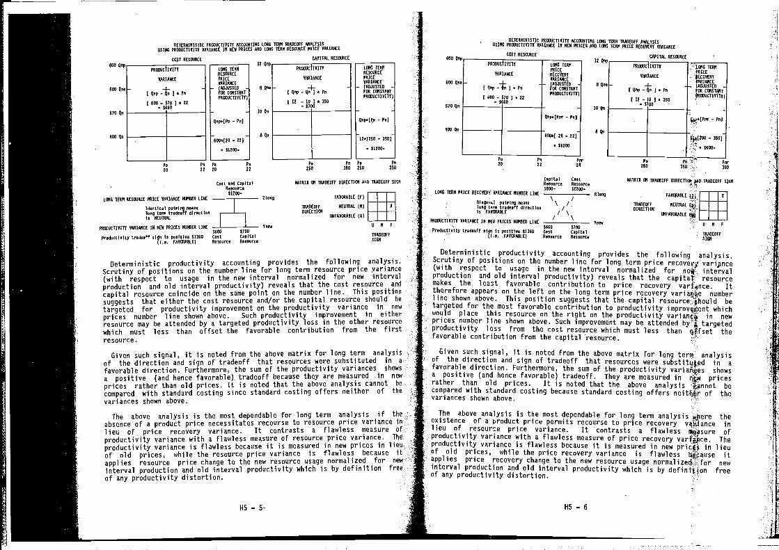
LUNG TERMRESOURCE
PRICERARIANCE(ADJUSTED -FUN CONSTANT
PROUUCTIRITT(
Deterministic productivity accounting provides the following analysis.Scrutiny of positions on the number line for long term resource price yariance(with respect to usage in the new interval normalized for new intervalproduction and old interval productivity) reveals that the cost resource and
capital resource coincide on the same point on the number line. This positionsuggests that either the cost resource and/or the capital resource should be
targeted for productivity improvement on the productivity variance in new
prices number line shown above. Such productivity improvement in eitherresource may be attended by a targeted productivity loss in the other resourcewhich must less than offset the favorable contribution from the firstresource.
Given such signal, it is noted from the above matrix for long term analysisof the direction and sign of tradeoff that resources were substituted in a
favorable direction. Furthermore, the sum of the productivity variances shows
a positive (and hence favorable) tradeoff because they are measured in new
prices rather than old prices. It is noted that the above analysis cannot be
compared with standard costing since standard costing offers neither of the
variances shown above.
The above analysis is the most dependable for long term analysis if theabsence of a product price necessitates recourse to resource price variance in
lieu of price recovery variance. It contrasts a flawless measure ofproductivity variance with a flawless measure of resource price variance. The
productivity variance is flawless because it is measured in new prices in lieuof old prices, while the resource price variance is flawless because itapplies resource price change to the new resource usage normalized for new
interval production and old interval productivity which is by definition freeof any productivity distortion.
Deterministic productivity accounting provides the following analysis.Scrutiny of positions on the number line for long term price recover1 vari?nce(with respect to usage in the new interval normalized for intervalproduction and old interval productivity) reveals that the capital resourcemakes the least favorable contribution to price recovery vart4nce. Ittherefore appears on the left on the long term price recovery numberline shown above. This position suggests that the. capital betargeted for the most favorable contribution to productivity improv ent whichwould place this resource on the right on the productivity in newprices number line shown above. Such improvement may be attended by targetedproductivity loss from the cost resource which must less than oSfset thefavorable contribution from the capital resource.
Given such signal, it is noted from the above matrix for long terra analysisof the direction and sign of tradeoff that resources were substituted in afavorable direction. Furthermore, the sum of the productivity varianães showsa positive (and hence favorable) tradeoff. They are measured in pricesrather than old prices. It is noted that the above analysis lannot becompared with standard costing because standard costing offers of thevariances shown above.
The above analysis is the most dependable for long term analysis theexistence of a product price permits recourse to price recovery inlieu of resource price variance. It contrasts a flawless ofproductivity variance with a flawless measure of price recovery varljpce. Theproductivity variance is flawless because it is measured in new pricfl in lieuof old prices, while the price recovery variance is flawless itapplies price recovery change to the new resource usage normalized. newinterval production and old interval productivity which is by definilion freeof any productivity distortion.
DETERMINISTIC PROUWCTI WIT? ACCOUNTING LONG TERM TRADEOPF ANALYSISRSING PROEOCIIVIIV VARIANCE IN MEW PRICES AND LUNG TERM RESOURCE PRICE VaRIANCE
CN$1 RESOURCE
PROUUCTI RITE
RONIANCE
(Qnp-tIaP,[ MOD — 57W 1 * 22
1660
600 gee
5lSWn
NeD i(o
W,pa(Po — P,,1
DETERMINISTIC PRONUCTIRITO ACCOUNTING LONG TERN TRADEWFF ANALTIISUSING PROURCTIRIOT RaDIANCE IN NEW PRICES AND LONG TEeN PRICE REC6RERT CARIANCE
CN$1 RESOURCECAPITAL RESOURCE
— 600'(lW — 22)
51200—
Po Po 7, Pc
2W 22 20 22
Coot and CapitalResourCe
51200—
LONG TERR WESOURCE PRICE VARIANCE WONDER LINE Ziong
Identical pairing mean,long Rena tradeoff directionI, NEUTRAL
PROUOCTIVITV VARIANCE IN NEA PRICES NUNRER LINE Inee1660 5700
ProduCtielty tradeoff sign iG po,itive 11365 Coot Capitol(i.e. FAUOUARLE( Resource Resource
PRmIUCIIRITT
RARIANCE
ERop-tIePo(12 — ID I ' 350
1700
UUO0n—. 12
PRXmCIIRITV LONG TERNPRICE
VARIANCE RECURERT
RARIANCENOD Rne . —)-- - (AUJORTED 0 Wee
(Rep — We J e Pc IOU CCNSTARTPROUUCTIAITV)
I dUO — 570 2 • 221660
SPORe - lOQe
gepalP,r — Pc]
WOOQe —
__________
. IQeUOOa( 24 — 22]
11200
Po Pc Per20 22 24
Capital CentRe,ource ResourcegROW— 51200—
LONG TERN PRICE RECOAERY AARIANCE NURSER LIRE Rlseg
pairing meano \ /long ten tradeoff direction /is FAVOUAOLE / \
PROEUCTIUITV VARIANCE IN OUR PRICES NUMBER LINE/
Veee1600 1700
Preductieity tradeoff sign io pesitiee 51360 Cost Capital(i.e. FAVOUASLE( Re,eurce Reseurce
LONG TERNtRICERECOVERYVARIANCE(ADJAUTED
CONSTANT
kPOCCACTIAITY
— Pn(
— 350]
- — gURU—
Pc? Per350 - 300
RWTRIA ON TRADEOFF DIRECTION AND TRADEOFF lIEN
FAVOUAOLE (F(
TRADEOFF REUTRAL (B] A
DIRECTIONURFAROUADLE (U)
UN F
TRADEOFF
SIGN
Pe
250
NUTRIA ON IRADEOFF MID TRADEOFF SIGR
- FAVOUARLE ifl1
TRADEOFF NEUTRALDIRECTION
_______
ANFARnERDLE
U N F
TRADEOFFSIGN
H5—5- -- H5—6
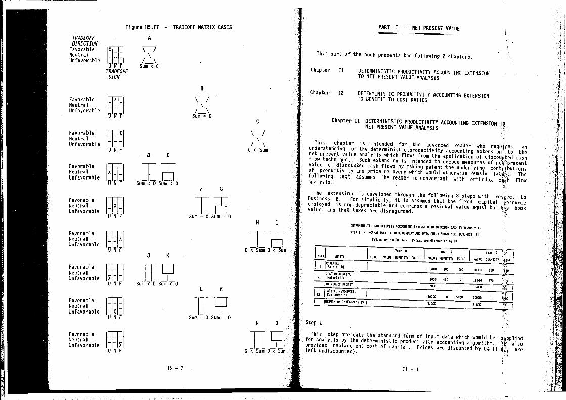
PART I — NET PRESENT VALUEFigure H5.F7 - TRADEOFF MATRIX CASES
TRADEOFF ADIRECTION
FavorableThis part of the book presents the following 2 chapters.Neutral \
Unfavorable — — —U Sum < 0
Chapter II DETERMINISTIC PRODUCTIVITY ACCOUNTING EXTENSIONTRADEOFFTO NET PRESENT VALUE ANALYSISSIGN
BChapter 12 DETERMINISTIC PRODUCTIVITY ACCOUNTING EXTENSION
TO BENEFIT TO COST RATIOSFavorableNeutral — —Unfavorable — -
u ii P Sum = 0Chapter Il DETERMINISTIC PRODUCTIVITY ACCOUNTING EXTENSION TQC
NET PRESENT VALUE ANALYSIS
HipFavorable —
— This chapter is intended for the advanced reader who an
Neutral — —
— understanding of the deterministic productivity accounting extension the
Unfavorable0 < SumU N P
net presept value analysis which flows from the application of cashD Eflow techniques. Such extension is intended to decode measures of
Favorable value of discounted cash flows by making patent the underlying contt1butionsNeutral of productivity and price recovery which would otherwise remain TheUnfavorable 1H IL analysis.following text assumes the reader is conversant with orthodox c4jh flowUNF Sum<OSum<O
F GThe extension is developed through the following 8 steps with toFavorable Business B. For simplicity, it is assumed that the fixed capital
NeutralUnfavorable '[II - employed is non-depreciable and commands a residual value equal to bookvalue, and that taxes are disregarded.
Sum = 0UN FH I
DETERMINISTIC PRaISCIIAITS ACCOUNTING EXTENSICM TN QQTN0005 CASH FLOW ANALYSIS
Favorable STEP I — NOUMUL HWE OF DATA DISPLAY ANN DATA ENT1IY SHOWN FCN NOSINESS NI
NeutralUnfavorable I YaToes are Is DOLLARS. PrIces are dlsceunEed by UN
OcSumO<SumJ
YearNJ
Yearl Year2U N FINSES ENTITY VERA VALUE QUANTITY PRICE VALUE QUANTITY PRICE AALYE QUANTITY FVCE
J K
REVENUE:
Favorable UI Shirts hiISUAS INS IOU 1850U 150Neutral
_______
Unfavorable [H II 25460
NI Nat,rIal hI0000 400 20 12540 570
INTRINSIC PNAFIT2000
UNF Sum<OSum<OL N CAPITAL RESOURCES:
01 EqutpmenL hI 40000 8 SAlON 70000 10IFavorable
NeutralUnfavorable HJI
5uJicUNF Sum = 0N 0 Stepl
Favorable This step presents the standard form of input data which would beNeutralUnfavorable provides replacement cost of capital. Prices are disounted by 0% are
for analysis by the deterministic productivity accounting algorithm. 14 also
O < Sum D C Som left undiscounted).UNF
ci Ii — 1115—7
L
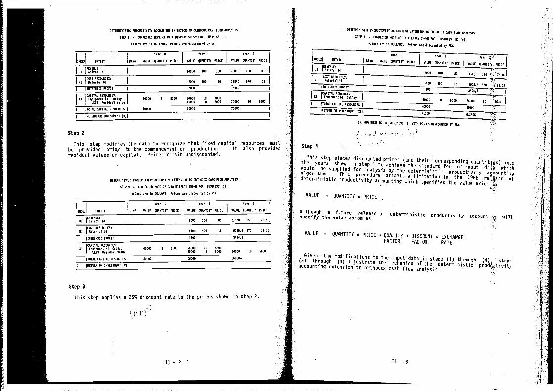
DETERMINISTIC PROSOCTIVITY ACCOUNTING EUTENSICNI 16 CAViOSOX CASH Flow ANALYSIS
STEP D — COURECTED NOSE OP DATA DISPLAY SHOW POU ROSINESS RI
Values are in DOLLAUD. Prices are discounted by IS
INDEX ENTITY
Tear 0 Year 1 Year 2
REVA VALUE QUARTITY PRICE VALUE QUARTITT PRICE VALUE QUANTITY PRICE
REVERIE:US Shirts bI
.
10000 100 III IR001 150 120
COST RESOURCES:
Ml Raterial bI 0000 401 20 12540 570 22
IIRTRSRSIC PROFIT 2110 5400
CAPITAL RESOURCES:Dl Equipment bI outlay
LESS Residual Value40000 N 5000 70000 II 7USD
40000 R S000 70000 10 7000
TOTAL CAPITOL RESOURCES 40000 30000 70000—
RETURN CR INOESTRERT (Oil
Step 2
This step modifies the data to recognize that fixed capital resources must
be provided prior to the commencement of production. It also providesresidual values of capital. Prices remain undiscounted.
DETERMINISTIC PROUHCTI VITO ACCOUNTING EXTENSIOS TO OSTHOSOU CASH PLON ARALYSIS
STEP 3 — COURECTCD NOSE OF DATA DISPLAY SHOW FOU ROSINESS RI
Values are In DOLLARS. Prices are discounted by 25%
INDEX ENTITY
Tear 0 Year I Tear 0
REVA VALUE QUORTITY PRICE AALOO QUANTITY PRICE VALUE QUANTITY PRICE
RERENUE:Ni Shirts hI WOO 100 NA 11020 150 76,0
COST RESOURCES:RI Raterial hI OAOX 600 SN 0A25,6 570 24,00
IINRVIN5IC PROFIT 2000 3RVR,4
CAPITAL RESOURCES:DI Equipment hi Outlay
LESS Residual Value40000 N SOVV 50000 10 5000
40000 N 5000 50000 10 5600
TOTAL CAPiTAL RESOURCES 40000 06000 50000—
I
Step 3
DETERRIVISTIC P0000CTiVITY ACCOUNTIRO EUTENSIOSTO OUTV0000 COON FLOU AVALYUIS
STEP 4 — COSRECTED NOSE OF DATA ENTRY SHOW POU ROSINESs RD (ai
Values are In DOLLARS. Prices are diocoonted by 250
VEVA VALUE QUANTITY PRICE VALUE QOARTITY PRICE I RALUE QUANTItY PUICE(
00 11020 250 760.!
MW 400 16 570 LAIR!
El Equipment hI Outlay40000 6 NOSY 56000 10
06000 -
I TOTAL CAPITAL REOCIJOCES:
:0:::6
OS IN RESIN
mi 00010050 RD ROSINESS N 67Th PRICED DISCOUNTED DV 25%
Step 4
I-f jJ t I
This step discounted prices (and their corresponding intothe years shown in step 1 to achieve the standard form of input data whichwould be supplied for analysis by the deterministic productivitya limitation in the 1988 rejgase ofdeterministic productivity accounting which specifies the value
a future release of deterministic productivity willspecify the value axiom as
VALUE = QUANTITY * PRICE * QUALITY * DISCOUNT * EXCHANGEFACTOR FACTOR RATE
Given the modifications to the input data in steps (1) through (4)a steps(5) through (8) illustrate the mechanics of the deterministicaccounting extension to orthodox cash flow analysis.
This step applies a 25% discount rate to the prices shown in step 2.
— 2
-I
II — 3
IL
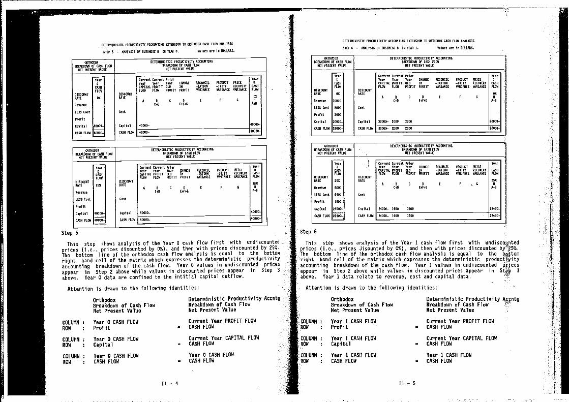
OWT00000RREAKARAN SF CASH FLAW
NET PRESENT VALUE
DETERMINISTIC PRCCIACTIYITY ACCOWNTINGBREAKDOWN OF CASH FLAW
NET PRESENT VALUE
AISCOWRTRATE
Revenue
LESS Cast
PraFiA
Capital
CASH FLOW
YearA
CASHFLAW
0%
4HAAA—
40000—
DISCERNTRATE
Cast
Capital
CASH FLOW
Current Current FriarYear Year Year CRRHGE YECENCIL PWAOACT PRICE
CAPITAL PRAFIT OLD IN —IATIOW —IYITY RECOVERY
FLAW FLOW PROFiT PROFIT VARIANCE RARIARCE YARIAHCE
A I C A E F A
Cvii E-vF+0
45uSD—
YearA
CASH
FLAW
ASH
AtH
4OAAS—
45500— 4ASAA—
OWTHOWAS
aREAKSAHN OF CASH FLOWNET PRESENT VALUE
DETERMINISTIC PROWACTIRSTY ACCOWNTIWOBREAKAOIRI SF CASH FLOW
NET PRESENT VALUE
DISCOWWTRATE
Revenue
LESS Caat
Fraf it
Capital
CASH FLOW
YearH
CASHFLOW
DNA
400A0—
40000—
DISCOWRT
RATE
Ceat
Capital
CASH FLOW
Current Current FriarYear Year Year CHANGE RECOWCIL P0055CY PRICE
CAPITAL PeAFIT ALA IN —IAYIOW —IHITT RECAYERY
FLOW FLOW PASFIT PROFIT HARIANCE VARIANCE YAROANCE
A I C 0 E F G
C+D E+FeG
AlIAS—
YearA
CASHFLAW
DUO
H
A+D
40000—
4ISAO— RAOEA—
Step 5
This step shows analysis of the Year 0 cash flow first with undiscountedprices (i.e., prices disounted by 0%), and then with prices discounted by 25%.The bottom line of the orthodox cash flow analysis is equal to the bottom
right hand cell of the matrix which expresses the deterministic productivityaccounting breakdown of the cash flow. Year 0 values in undiscounted prices
appear in Step 2 above while values in discounted prices appear in Step 3
above, Year 0 data are confined to the intitial capital outflow.
Attention is drawn to the following identities:
OWTAOWOA
BRE000ARWI OF CASH FLOW
NET FRESENY HALRE
DETERMINISTIC PRtOACTIYITY ACCOWNTIN0BREAKDAWN OF CASH FLOW
NET PRESENY VALUE
DISCOWNT
RATE
Revenue
Year1
CASHFLOW
DO
11111
DISCOHNTRATE
Current Current FriarYear Year Year CHAHGE RECOWCIL
CAPITAL PROFIT ALD IN —IATIOWFLOW FLOW PROFIT FROFIT YOWIANCE
A B C 5 0
Cvii EvFeG
FIOWACT
—IOSTYYARSANCE
F
FRICERECAAERYVARIANCE
I
YearI
CASA
FLOW
OW
A
0-va
LESS Cast RAIN Cast
PraFit 2050
Capital
CASH FLOW
30000—
2OWAA—
Capital
CASH FLOW
30000— DIII 2000 DaAIY—
3000W— 1100 1100 20000—
00THRREAKSSNN
HEY FRES
0000IF CASH FLOWWT OALAE
DETERMINISTIC FROWACTIOITT ACCOWNTINGBREAKDOWN RF CASH FLOW
NEY PRESENT RALUE
Year - Current Curraht Friar Year•
I Tear Year Year CRANOE RECOWCIL FROWACT PRICE I
CASH CAPITAL PROFIT OLD 1R —IATIOW —IKITY RECOISRY CASH
FLOW FLOW FLOW PROFIT PROFIT VOWIANCE HOWIANCE VOWIANCE FLOW
DISCOWNT SDSCOWHT
RATE 150 RATE ORG
Revenue 000WA I C S E
E+F+0F H
AvG
LESS Cast
Frafit
640W
1600
CaaO B
1
Capital
CASH FLOW
14010—
22400-
CvpiOii
CASH FLOW
14111— SAIl 1601 12450—
D4050— IAOO 1600 DD4AI—
Step 6
This step shows aralysis of the Year 1 cash flow first with undiscozwltedprices (i.e., prices Jisounted by 0%), and then with prices discounted bfls%.The bottom line of the orthodox cash flow analysis is equal to theright hand cell of the matrix which expresses the deterministic productjwityaccounting breakdown of the cash flow. Year 1 values in undiscounted ptlcesappear in Step 2 above while values in discounted prices appear in Stag 3
above. Year 1 data relate to revenue, cost and capital data.
Attention is drawn to the following identities:
- RETERMIBISTIC PROWUCTIHITY ACCOWNTINO ESTERSIOW TO OWTHOWAO CASW FLOW ARALYSIS
STEP S — ANALYSIS OF IRSINESS B SN TEAR A. Yalaea are 1' DOLLARS.
DETERNINSDTIC FROWOCTIRIIT ACCOWWTINI ESTENOSOW TA OW1WOWOS CASH FLOW ARALYSIS
STEP 6 — OWALYSIS OF BASINESS B IN YEAR I. Values are in DOLLARS.
OrthodoxBreakdown of Cash FlowNet Present Value
COLUNN : Year 0 CASH FLOWROW Profit
COLUMN : Year 0 CASH FLOWROW : Capital
COLUMN Year 0 CASH FLOWROW CASH FLOW
Oeterministic Productivity AccntgBreakdown of Cash FlowNet Present Value
Current Year PROFIT FLOW— CASH FLOW
Current Year CAPITAL FLOW— CASH FLOW
Year 0 CASH FLOW— CASH FLOW
COLUMN
ROW
OrthodoxBreakdown of Cash FlowMet Present Value
Year I CASH FLOWProfit
— 4
COLUMN : Year 1 CASH FLOW- ROW Capital
COLUMN
ROW
Oetermlnlstlc ProductivityBreakdown of Cash FlowMet Present Value
Current Year PROFIT FLOW— CASH FLOW
Current Year CAPITAL FLOW— CASH FLOW
Year 1 CASH FLOW— CASH FLOW
Year 1 CASH FLOWCASH FLOW
II — 5
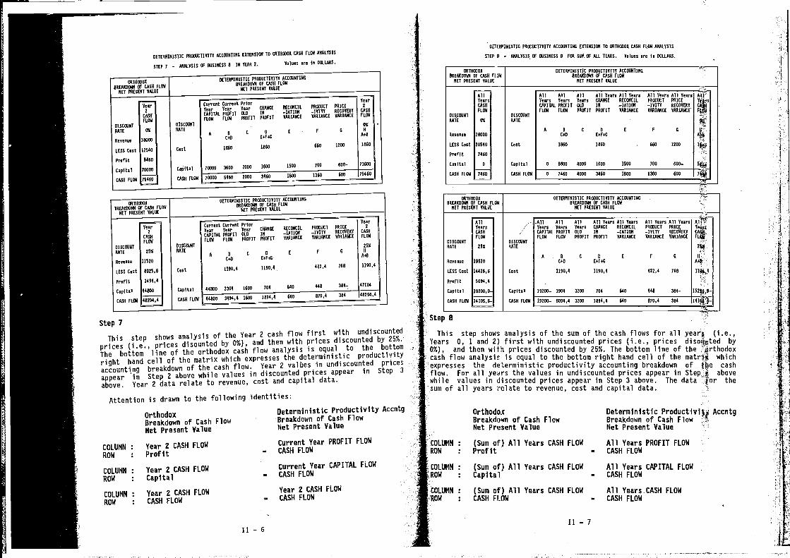
DETERMINISTIC PRAROCTIVITO HCCCGNTIHG ESTENSIOW TO OWSHAROU CASH nON ANALYSIS
STEP 7 — ANALYSIS OF NOSINESS B IN YEAR 2. values are In DOLLARS.
DETERMINISTIC PV000CIIYITT HCCOWNTIHGNR00000IHI or CASH FLOW
NET PRESENT VALHE
Current Current PrIorYear
Year Year Year CHANGE PROWOCT PRICE 2
CAPITAL PROFIT OLD SW —IATI&i —lAITY RECOYERY CASH
FLOW PLON PROFIT PROFIT HHRIARCE YARIARCE VARIANCE PLOH
ARTOAROSDETERNINISIIC POSHOCTIRITH ACCOUNTIWS
BREAKDOWN HF CASH PLeABREAKDOWN OF CAIN FLOW
NET PRESEWY YALHENET PRESENT HALSE
Year
ID 2
I CASH
CASH
I FLOHFLRH
DISCOWOT I DISCOWNO
PATE I 25% RATE
25%
I A N C B EA
Revenue 111520C-sO E+F+G
0+0
LESS Cest 8025,6 Cost 1100,4 1100,4 402,4 7H8 1500,4
PrnFlt 3404,4
Capital 44001
___________________________________________________________
CASH FLOW HHDR4.4
CWOTOCKIOO
BREAKDOWN OF CHOW FLOW
WET PRESENT YHLHE
Year
CASHFLOW
DISC RANT
lATE NA
Renanue 10000
LESS Cnst 12540
ProF It SNNN
CaplRal 70000
CASH FLOW 7SWAO
DETERMINISTIC PRRAOCTOA1IT ACCOWNTIWS EXTENSION TO 001110000 CAIN FLOW ANALYSIS
STEP 8 — ANALYSIS OF BUSINESS N VOW SON OF ALL YEARS. Values are In DOLLARS.
DISCOUNT
RATE0%
A B C I E - F G W
CeO E+F+RA+N
Cost 1800 1060 660 1200 1800
CapItal 70000 3600 2000 1000 1500 700 600— 73600
CASH FLOW 70000 N4NO 2000 3400 1500 1360 608 7S400
torrent Current PrIorYear Tear Year CHRNSE RECOWCSL PROWACT PRICE
CAPITAL PROFIT OLI IN —DATIOW —lAITY RECOYERY
FLOW PLOW PROFIT PROFIT VARIANCE YORIORCE VARIANCE
F C
OWTROWOU
NREAKOOWN OF CASH FtNET PRESENT RALNE
— DETERMINISTIC PROWOCTIVITY ACCOWNTIWO30 DREOKDOAN OF CASH FLOW
NET PRESENT NALOE
AllYearsCASW
FLOW
DISCOWNTDATE AR
Rooenoe 20000
LESS Cost 20540
ProFit 7460
CapItal 0
CAIN FLOW 7460=-
All All All HID Years All Teara All Tears All YearsTears Years Years CHANGE RECOWCIL PRAROCT PRICE YCosCAPITAL PROFIT OLO IN —IHTIOW —1051'! RECOVERY
FLOW FLOW PROFIT PROFIT VARIANCE VARIANCE VARIANCEDISCOUNTRATE
A 8 C D E F 6 irC+D E+FaG
Cost 5000 1800 - 660 1200
I SHOA 4000 1600 1500 700 600—
CHOW FLOW I 7460 4000 3460 1500 5360 600 744k=—
OWTOOWOO
BREAKDOWN OF CASH FLOVNET POESENT RALHt
- - DETERNINIOTIC PROWOCTI PITT ACCOUNTINGBREAKDOWN OF CAIN FLOW
NET PRESENT VALUE —
DIOCOWNT
RATE
Revanoe
LESS Cost
ProfIt
Capital
CASH FLOW
AllYearsCASH
FLOW
25%
10520
14425,6
5004,4
58200,0-.
54105W..
,
DISCOWNT
RATE
Cost
Capital
CASH FLOW
.
—All All All All Years All Tears All Years All YearsTears Years Years CHARGE RECOWCIL POOWOCT PRICECAPITAL PROFIT OLD IN —IWIIOW —IRITT RECROERY
FLOW FLOW PROFIT PROFIT VARIANCE RARIANCE RARIANCE
A N C D E F K
Cell E+F+G
5100,4 1110,4 422,4 768
11200— 3004 3200 704 640 448 304—
CA01+
,--
0.
-
10200— 5004,4 3200 5004,4 N4H 870,4 380
CapItal 44000 2304 1600 704 640 440 304— 47104
CASH FLOW 5448003484.4 1000 1804,4 640 870,4 304 40294,4
Step 7
This step shows analysis of the Year 2 cash flow first with undiscounted
prices (i.e., prices disounted by 0%), and then with prices discounted by 25%.
The bottom line of the orthodox cash flow analysis is equal to the bottom
right hand cell of the matrix which expresses the deterministic productivity
accounting breakdown of the cash flow. Year 2 valUes in undiscounted prices
appear in Step 2 above while values in discounted prices appear in Step 3
above. Year 2 data relate to revenue, cost and capital data.
Attention is drawn to the following identities:
- Step 8
This step shows analysis of the sum of the cash flows for all years (i.e.,Years 0, 1 and 2) first with undiscounted prices (i.e., prices by0%), and then with prices discounted by 25%. The bottom line of the jrthodox
- cash flow analysis is equal to the bottom right hand cell of the matr-}j whichexpresses the deterministic productivity accounting breakdown of tbe cashflow. For all years the values in undiscounted prices appear in Step 4 abovewhile values in discounted prices appear in Step 3 above. The data Lor thesum of all years relate to revenue, cost and capital data.
OrthodoxBreakdown of Cash FlowNet Present Value
COLUMN Year 2 CASH FLOWROW Profit
COLUMN Year 2 CASH FLOWROW : Capital
COLUMN Year 2 CASH FLOWROW CASH FLOW
Deterministic productivity AccntgBreakdown of Cash FlowNet Present Value
Current Year PROFIT FLOW— CASH FLOW
Current Year CAPITAL FLOW— CASH FLOW
Year 2 CASH FLOW— CASH FLOW
OrthodoiBreakdown of Cash FlowNet Prusent Value
- COLUMN
ROW
Deterministic Productlvltg AccntgBreakdown of Cash FlowNet Present Value
COLUMN : (Sum of) All Years CASH FLOW All Years PROFIT FLOW -
ROW Profit — CASH FLOW
Ii — 6
(Sum of) All Years CASH FLOWCapital
COLUMN (Sum of) All Years CASH FLOWROW CASH FLOW
Ii — 7
All Years CAPITAL FLOW— CASH FLOW
All Years.CASH FLOW— CASH FLOW
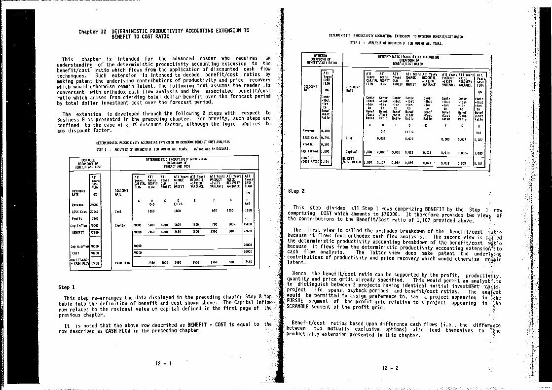
Chapter 12 DETERMINISTIC PRODUCTIVITY ACCOUNTING EXTENSION TOBENEFIT TO COST RATIO
This chapter Is intended for the advanced reader who requires an
understanding of the deterministic productivity accounting extension to thebenefit/cost ratio which flows from the application of discounted cash flowtechniques. Such extension is intended to decode benefit/cost ratios by
making patent the underlying contributions of productivity and price recoverywhich would otherwise remain latent. The following text assumes the reader Asconversant with orthodox cash flow analysis and the associated benefit/costratio which arises from dividing total dollar benefit over the forecast periodby total dollar investment cost over the forecast period.
The extension is developed through the following 2 steps with respect toBusiness B as presented in the preceding chapter. For brevity, such steps areconfined to the case of a 0% discount factor, although the logic applies toany discount factor.
DETERMINISTIC PRONUCTI VIII ACCOUNTING EXTENSImI TO OWThWAO BENEFIT COST ANALYSIS
STEP I — ANALTSIS OF BUSINESS B FOB SUM OF ALl. YEARS. Values are In DOLLARS.
OWTSOOIOO
IREA000IVI OFBENEFIT AND COST
SETESNINISTIC P0000CTI VIII ACCOUNTINGBRE00500N OF
BENEFIT AND COST
DISCeVITRATE
AllYearsCAlMFLOW
0%
DISCOUNT
RATE
All an all All Yeara All TearsYears Years Tears CAYNGE RECOWCIL
CAPITAL PROFIT OLD IN —IASSOW
FLOW FLOW PROFIT PROFIT VARIANCE
All Years All YearsPROWUCT PRICE—lAITY RECOVERT
VARIANCE VARIANCE
AllYearsCASO
FLOW
5%
Veeeeue D000V
A B C S E
CeO [WoOF 0 V
Aol
LESS Cest 26540 Cast 1000 IONS 005 1100 INNS
PraY It 740S .
Cap InFlow
BENEFIT
Cap OutFlow
COST
ENEFIT-COST= CASH FLOW
10000
77400
70000
7V555
7460
Capital
CASN FLOW
70000 BUSS 400S 1600 1000 700 000— 75600
10000 7400 4000 340S SBUS 130S 005 77600
70000 70000
70000 70005
7400 400S 3460 1500 1301 005 7460
Step I
This step re—arranges the data displayed in the precedingtable into the definition of benefit and cost shown above.row relates to the residual value of capital defined in theprevious chapter.
It is noted that the above row described as BENEFIT - COST is equal to therow described as CASH FLOW in the preceding chapter.
DETEVNINISTVC PROWOCTIVITY ACCOUNTING ESTENSIOW TO OWI1IOWOX BENEFIT/COST RATIO
STEP 2 — ANALYSIS OF BUSINESS B FOW SUN OF ALL YEARS.
BREAKDOWN OF
BENEFIT/COST RATIO
POOWOCTIVSTT ACCOUNTINGDRE0000IN OF
BENEFIT/COST RATIO
AllYearsCASA
FLOWOSSCmINTRATE OW
tonEr—Ibet—lenLa
Bene?/CsotRatio
Nenenue 0.400
LESS Cost 0,203
ProFIt 0,107
SSCOWNT
YAlE
Cost
All All All 011 Years 011 YearsYears Years Tears CHANGE OECOWCILCAPITAL PROFIT OLD IN —IATSOWFLOW FLOW PROFIT PROFIT VOWIANCE
Contr Cootr Centr Contr CanEr-Ibut —Ibat —Ibat —Ibat —IbaE—lan —Ion —Ion —Ian —Ianto On ta to to
Dccc? Ieee? Bane? Bone? lene?/Cost /Coot /CoaE /Cost /CesORatio RatIo Ratio RatIo Ratio
A B C 0 E
CoO EoF+G
0,027 0,026
All Tears All YsursPRODUCT PRICE—IVITT RECOVERYVARIANCE VARIANCE
-
CanEr CanEr—IbuE —lUst—Ion —Ionto to
lone? Ieee?/Cost /CastRatIo RatIo
F 6
0,000 0,017
All-TearsCASH
FLOW
NO
Centr—Ibut—Ianto
lone?/CostDatla
V
A+B
0,027
-
Cap InFloaq 1,000
BENEFIT/COST RATIO 1,107
CapItal
BEIIEFIT/COST RATIO
1,000 0,000 0,050 0,023 0,021 0.010 0,006— I,OOW
1,000 6,107 0,050 0,641 0,021 - 0,011 0,000 1,107
Step 2
This step divides all Step I rows comprizing BENEFIT by the Step 1 rowcomprizing COST which amounts to $70000. It therefore provides two ofthe contributions to the Benefit/Cost ratio of 1,107 provided above.
The first view is called the orthodox breakdown of the benefit/cost rflio Hbecause it flows from orthodox cash flow analysis. The second view is cOledthe deterministic productivity accounting breakdown of the benefit/cost i'4tiobecause it flows from the deterministic productivity accounting tocash flow analysis. The latter view does make patent thecontributions of productivity and price recovery which would otherwise rel$ainlatent.
Hence the benefit/cost ratio can be supported by the profit,quantity and price grids already specified. This would permit an analyst toto distinguish between 2 projects having identical initial inve$tiheiTt—-—Rons,project life spans, payback periods and benefit/cost ratios. The anajystwould be permitted to assign preference to, say, a project appearing in
the profit grid relative to a project appearing inSCRAMBLE segment of the profit grid.
Benefit/cost ratios based upon difference cash flows (i.e., the differodcebetween two mutually exclusive options) also lend themselves to ?lheproductivity extension presented in this chapter.
12—112 — 2
chapter Step 8 topThe Capital Inflowfirst page of tho
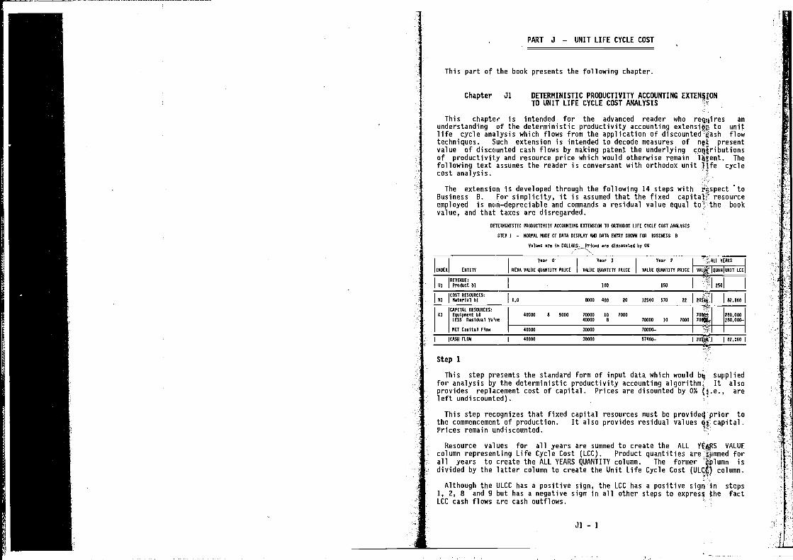
PART J — UNIT LIFE CYCLE COST
This part of the book presents the following chapter.
Chapter Ji DETERMINISTIC PRODUCTIVITY ACCOUNTINGTO UNIT LIFE CYCLE COST ANALYSIS
This chapter is intended for the advanced reader whounderstanding of the deterministic productivity accounting to unitlife cycle analysis which flows from the application of discounted flowtechniques. Such extension is intended to decode measures of presentvalue of discounted cash flows by making patent the underlying contributionsof productivity and resource price which would otherwise remain 4tent. Thefollowing text assumes the reader is conversant with orthodox unit cyclecost analysis.
The extension is developed through the following 14 steps withis assumed that the fixed capital resource
employed is non—depreciable and commands a residual value equal bookvalue, and that taxes are disregarded.
DETERMINISTIC PRODUCTIVITY ACCOUNTING EXTENSION TO ONTHODOS LIFE CYCLE COST ANALYSIS
STEP I — NORItAL MODE OF DATA DISPLAY AND DATA ENTRY SNUbRI FOD BUSINESS B
Values are DOLLARS. Prices are discounted by 0%
Year 0 Year I Year 2 YEARS
INDEX ENTITY
REVENUE:
UI Product bi
VERA VALUE QUANTITY
•
PRICE VALVE QUANTI
100
TV PRICE VALUE QUARTITY
INN
PRICE ICC
250
COST RESOURCES:
NI Material bI 1,0 OOUO 400 20 12540 57N 22 82.160
CAPITAL RESOURCES:El Equipsaent bI
LESS Residual Vaoe
RET Capital Flow --ICASN FLOW I--
40000 N 5000 10000 1040000 8
100070000 10
I
7000 70i0$.r280,000280,000—
40000
40000
30000
30000
70U00—
57460—
T
I 82,160 I
Step 1
This step presents the standard form of input data which would suppliedfor analysis by the deterministic productivity accounting algorithm. It alsoprovides replacement cost of capital. Prices are disounted by 0% (i.e., areleft undiscounted).
This step recognizes that fixed capital resources must be provided prior tothe commencement of production. It also provides residual values capital.Prices remain undiscounted.
Resource values for all years are summed to create the ALL VALUEcolumn representing Life Cycle Cost (LCC). Product quantities are forall years to create the ALL YEARS QUANTITY column. The former isdivided by the latter column to create the Unit Life Cycle Cost column.
Although the ULCC has a positive sign, the LCC has a positive in steps1, 2, 8 and 9 but has a negative sign in all other steps to express factLCC cash flows cash outflows.
— 1
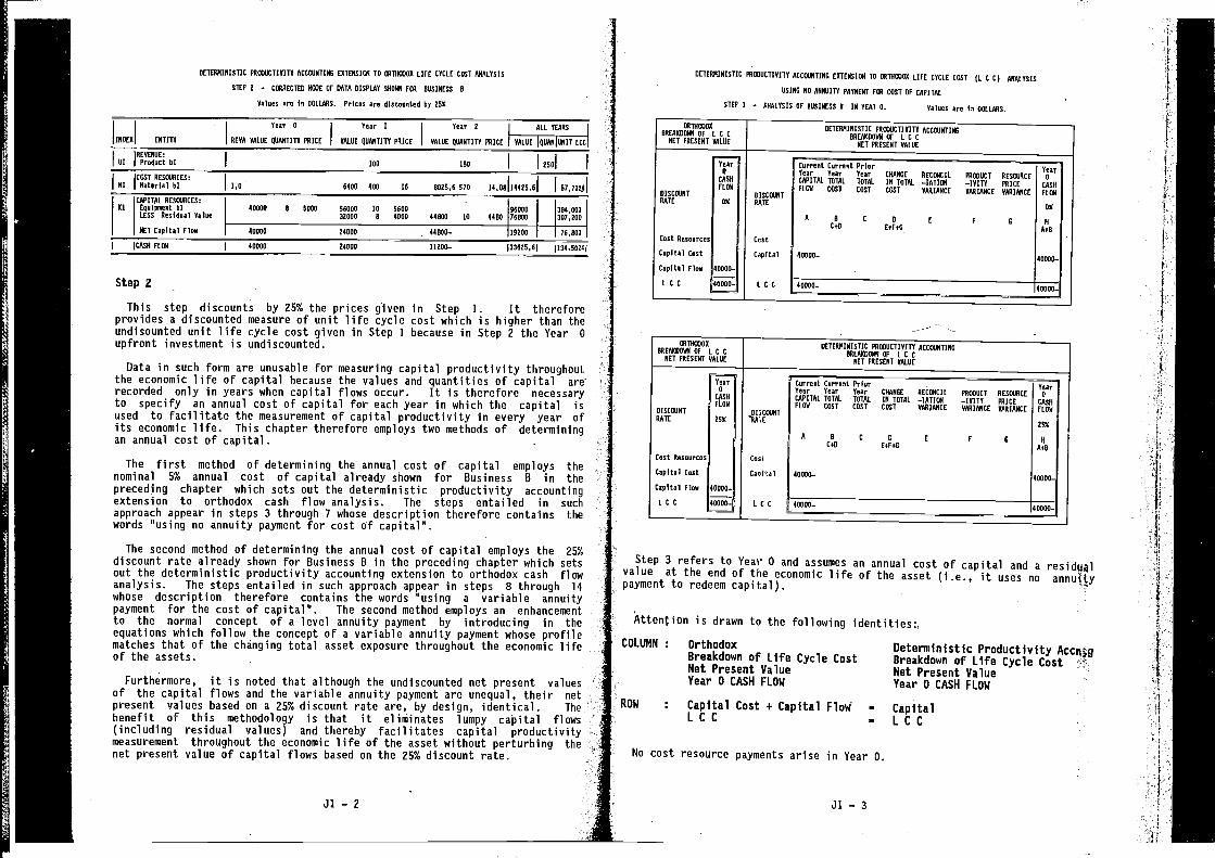
DETERMINISTIC PROSUCTI VITO ACCOUNTING EOTENSIcN1 TO DATROSOS LIFE CYCLE COST ANALYSIS
STEP 2 — CmOECTEI NOSE OF DATA DISPLAY S1I0AR FDA ROSINESS
Yalses are in DOLLARS. Prices are discoa,ted by 25%
INRER ENTITY RERA VALUE
Tear 0
QUANTITY PRICE
Sear
VALUE ROANT
1
ITT PRICE
Year 2
VALUE QUANTITY PRICE
ALL YEARS
VALUE QUANJARIT LCC
REVENUE:Dl Predact hi III ISO 250
EOST RESOURCES:NI Material hi 1,0 6400 400 16 0025,6 570
)
14,00)14425,61 57,7S2j
ElCAPITAL RESOURCES: I
EqaipmeaL hiI
LESS Residaal Yalsa
NET Capital Flow
40000
40000
8 5000 56000 1032000 8
24UVA
50004000
.
44800 10
44800—
4400
I
NOV0076800
p
102A0 f
I
384,000I
307,200
—
Step 2
This step discounts by 25% the prices givenprovides a discounted measure of unit life cycleundisounted unit life cycle cost given in Step 1upfront investment is undiscounted.
Data in such form are unusable for measuring capital productivity throughoutthe economic life of capital because the values and quantities of capital arerecorded only in years when capital flows occur. It is therefore necessaryto specify an annual cost of capital for each year in which the capital isused to facilitate the measurement of capital productivity in every year ofits economic life. This chapter therefore employs two methods of determiningan annual cost of capital
The first method of determining the annual cost of capital employs thenominal 5% annual cost of capital already shown for Business B in thepreceding chapter which sets out the deterministic productivity accountiVgextension to orthodox cash flow analysis. The steps entailed in suchapproach appear in steps 3 through 7 whose description therefore contains thewords "using no annuity payment for cost of capital".
The second method of determining the annual cost of capital employs the 25%discount rate already shown for Business B in the preceding chapter which setsout the deterministic productivity accounting extension to orthodox cash flowanalysis. The steps entailed in such approach appear in steps 8 through 14whose description therefore contains the words "using a variable annuitypayment for the cost of capital". The second method employs an enhancementto the normal concept of a level annuity payment by introducing in theequations which follow the concept of a variable annuity payment whose profilematches that of the changing total asset exposure throughout the economic lifeof the assets.
Furthermore, it is noted that although the undiscounted net present valuesof the capital flows and the variable annuity payment are unequal, their netpresent values based on a 25% discount rate are, by design, identical. Thebenefit of this methodology is that it eliminates lumpy caØital flows(including residual values) and thereby facilitates capital productivitymeasurement throughout the economic life of the asset without perturbing thenet present value of capital flows based on the 25% discount rate.
OUTNOSOY
BREAKDOWN OF L C CNET PRESENT VALUE
DETERMINISTIC POOSUCTIVITYDVEA0000N OF I C C
NET PRESENT VALVE
ACCmNTINS
DISCOUNTRATE
Year0
CASH
FLOW
IXDISCOUNTRATE
Carre,t Carre,t PrierYear Taar Year CHANGECAPITAL TOTAL TOTAL IN TOTALFLOW COST COST COST
RECONCIL
—IAT1S81
VARIANCE
PROSOCT
—lAITYVARIANCE
RESOURCE
PRICEVARIANCE
Year0
CASH
FLOW
A D C ICaR [WaG
E F 0
0%
N
Cost Researcea Ccet
AtO
Capital Cast Capital 40000—
Capital Flow
LCC
40000-
40000— LCC
40000—
40000—40000—
OUTVmIOSOREAKO VON HF L C C
NET PRESENT VALUE
— DETERMINISTIC PROSOCTIVITYDREAKO VAN OF L C C
NET PRESENT VALUE
ACCOUNTING
YearV
CASH
FLOA
Carreot Carreet PriorYear Year Year CHANGECAPITAL TOTAL TOTAL IN TOTALFLOW COST COST COST
RECOWCIL—IATIONVARIANCE
PRVOSCT
—lAITYVARIANCE
RESOURCE
PRICEVANIANCE
TearU
CASHFLOWDISCOUNT
RATE 25%DISCOUNT
A 8. C 0CaR [eFaG
E P 0
255
U
Coot Reeaarceo Cast
Capital Coat CapRal 40000—
Capital Flow
ICC40000—
0%000- LCC
40000—
fl140000-
Step 3 refers to Year 0 and assumes an annual cost of capital and avalue at the end of the economic life of the asset (i.e., it uses no annuitypayment to redeem capital).
Attention is drawn to the following identities:,
DETERMINISTIC P0000CTIVITY ACCOUNTING ESIENSIm4 TO milimloo LIFE CYCLE COST )L C C) ANALYSIS
USING 00 ANNUITY PATNENT FOU COST OF CAPITAL
sTEP 3 — ANALYSIS OF BUSINESS B IN YEAH H. Valaaa are I, GOLLARD.
in Step 1. It thereforecost which is higher than thebecause in Step 2 the Year 0
COLUMN OrthodoxBreakdown of Life Cycle CostNet Present ValueYear 0 CASH FLOW
ROW Capital Cost + Capital FloW —
LCC —
No cost resource payments arise in Year 0.
JI — 3J1—2
i
Deterministic Productivity AccrqgBreakdown of Life Cycle CostNet Present ValueYear 0 CASH FLOW
CapitalLCC
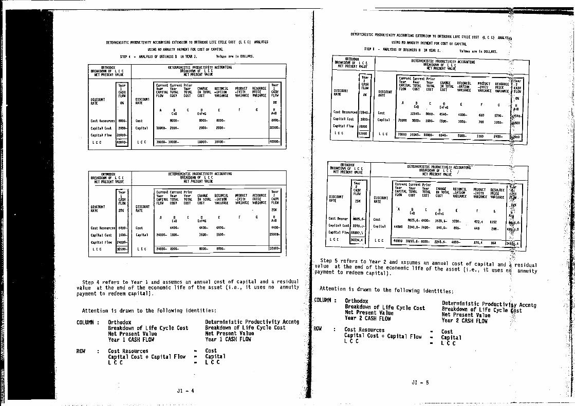
DETERMINISTIC PRUROCTIVITT ACCOUNTING EATENSIOW TO OUThUROX LIFE CYCLE COST (L C C) ANALYSIS
USING NO ANNUITY PAYMENT FOU COST OF CAPITAL
STEP 4 — AJIALYSIS OF NOSINESS U IN YEAR I. Values are In DOLLARS.
OU10C000NREA0001NIOF LCC
NET PRESENT VALUE
OETERNINISTIC PNCOUCTI VITA ACCOUNTINGNREA000hNOF LCC
NET PRESENT VALUE
DISCOUNTRATE
Cent Rennurcen
Capital Cant
Capital Flow
L C C
YearI
CASN
FLOW
0%
0011—
2000—
30000—
40000—
DISCOUNTRATE
Cost
CapItal
1 C C
Current Current PrierTear Teur Year CAANGE RECOWCIL PROSUCT RESOURCE
CAPITAL TOTAL TOTAL IN TOTAL —IAIICN —I VITA PRICE
FLOW COST COST COST VARIANCE VARIANCE VARIANCE
A I C S E P 0
CuD EFaG
0000— 0001— 0000—
30001- 2000— 2000— 20A0—
YearL
CATSV
FLOW
0%
A
0-el
0050—
32000—
30000— 10000— 10000— 10000— 40000—
OUTYOSOO
NREAE200N OF L C CNET PRESENT VALUE
DETERMINISTIC PR000CTIYITT ACCOUNTINGNREAEOO¾N OF L C C
NET PRESENT VALVE
DISCOUNTRATE
Coot Resources
Capital Coot
Capital Flow
ICC
YearI
CASR
FLOW
25%
0000—
IANO—
24000—
32000—
DISCOUNT
RATE
Cost
Capital
LCC
Current Current PrierTear Your Tear CNANGE RECOUCIL POOUUCT RESOURCE
CAPITAL TOTAL TOTAL IN TOTAL —IATIOW —IYITT PRICE
PLON COST COST COST VARIANCE VARIANCE VARIANCE
.
A U C I E F G
CuD E+EoD
0400— 6400-. 0400—
20000— 1000— 1000— 1000—
Tear1
CASV
FLOA
25%
N
A+l
6400—
25601-
24000— 0000— 0000— 0000— 32000—
Step 4 refers to Year I and assumes an annual cost of capital and a residualvalue at the end of the economic life of the asset (i.e.0 it uses no annuitypayment to redeem capital).
Attention is drawn to the following identities:
COLUMN Orthodox Deterministic Productivity AccntgBreakdown of Life Cycle Cost Breakdown of Life Cycle CostNet Present Value Net Present ValueYear 1 CASH FLOW Year 1 CASH FLOW
ROW Cost ResourcesCapital Cost + CapitalLCC
Flow—
a—
CostCapitalLCC
-
CHANGE RECOWCIL PROUOCT RESOURCE M 2IN TOTAL —IATIOW —IVITY PRICE t CASVCOST COST VARIAACE RARIANCE VARIANCEf FLOW
[NoE F 0 --to
4000— 660 1200— U,N40_1000- 700 2200— 500
7000020040— 20000— 6040— 5000— I3NO 2400—
Capital -
LCC
Current Current PriorTear Tear Year CHANGE VECOWCIL PREOUCT UESEEJVCECAPITAL TOTAL TOTAL IA TOTAL —IATIOW —lAITY PRICE toyiFLOW COST COST COST VARIANCE AAJ1IANCE VARIANCE
0-'
410*0
3Nfl,4
Step 5 refers to Year 2 and assumes an annual cost of capital and residualvalue at the end of the economic life of the asset (i.e.n it uses nà annuitypayment to redeem capital).
DETEOtNIOTIC PVOUUCTI 0211 ACCOUNTING EATENSIOW TO OUOUOUOV LIFE CTCLE COST (I C C) ANALTSfl
USING HO ANNOIIT PAVUENT FUR COST GF CAPITAL
STEP S — ANALYSIS OF NOSINESS I IN TEAS 2. Values are In DOLLARS.
00100000DETEONINI5TIC FROUOCTJR2TT ACCOUNTINGNREA020NN OF L C C
RVEA000IVI OF L C CNET PRESENT VALVENET PRESENT VALUE
N C SC-au Eu-P 4
12540- 0000- 4540-
7000N 3500— 2V00— 1500—
DETERNINISTIC POOUOCTIVITT ACCOUNTINGROEAKDOAN OF L C C
NET PRESENT VALUE -
LCC
A I C 2CuD Eu-FoG
NO2N.N— 6400— IO2N,6— 3200—
44000 2240,0— 1000— 640,0— 000—
E F 0
422,4 1252
440 200-
44RVA 10205,0— 0000— 2265.0— 4000— 070,0 064
Ji — 4
Attention is drawn to the following identities:COLUMN : Orthodox Deterministic AccntgBreakdown of Life Cycle Cost Breakdown of Life CycleNet Present Value Met Present Value
Year 2 CASH FLOW Year 2 CASH FLOW
ROW Cost Resources— Cost
Capital Cost + Capital Flow — CapitalLCC— LCC
Ji — 5
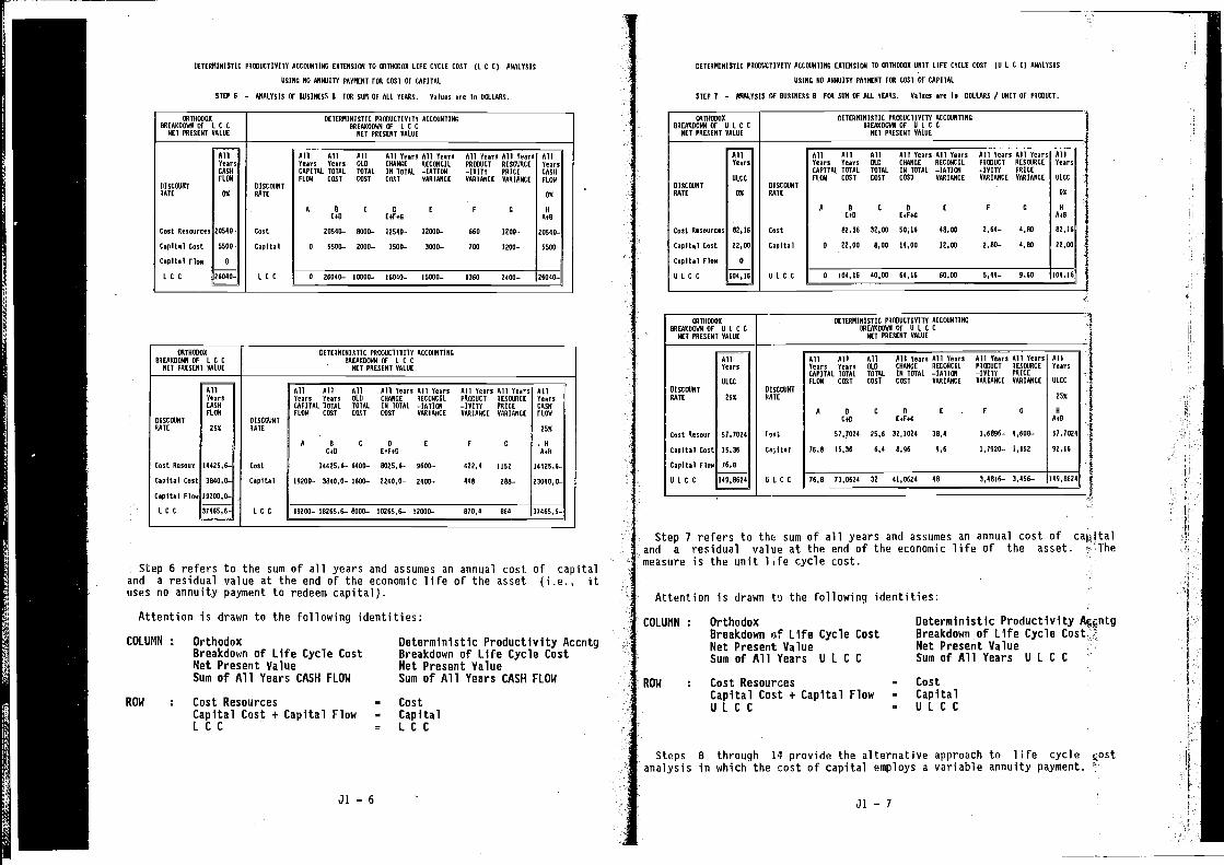
COLUMN OrthodoxBreakdown of Life Cycle CostNet Present ValueSum of All Years CASH FLOW
ROW Cost ResourcesCapital Cost + Capital FlowLCC
Oeterministic Productivity AccntgBreakdown of Life Cycle CostNet Present ValueSum of All Years CASH FLOW
= Cost— Capital= LCC
COLUMN OrthodoxBreakdown Gf Life Cycle CostNet Present ValueSumof All Years ULCC
ROW Cost ResourcesCapital Cost + Capital FlowULCC
— Cost— Capital• ULCC
DETERMINISTIC PROUOCII VITO ACCOUNTING ENTENSIOW TO OUIOOUOA LIFE CYCLE COOT )L C C) ANALYOIO
00260 NO A000ITY PAYMENT FOR COST OF CAPITAL
STEP 6 — ANALYSIS OF 20510ES5 N PEN SON OF ALL TEARS. Aalaes ore In DOLLARS.
DETERNINISTOC PROUOCTIRITT ACCOUNTING ETTENSIIAI TO OWTNOUOO OMIT LIFE CYCLE COST 10 L C C) ANALYSIS
05105 NO ANNOITT PAYMENT FEll COST OP CAPITAL
STEP 7 — NIALYSIS OP ROSINESS N rm SON OP ALL TEARS. Values are in DOLLARS / OMIT OF PNOSOCT.
01100100NOE0000VNI OF I C C
NET PRESENT YALNE
DETERMINISTIC PROUOCTIYITY ACCOUNTINGOREA000NAI OF I C C
NET PRESENT YALOE
AllTearsCASN
FLOW
DISCOUIITRATE OS
Cast Resources 20540—
Capital Cast 5500-.
Capital Plsw A
C C 26040—
DISCCAJNT
RATE
Cast
Capital
L C C
AlT All All All Years All Years All Tears All TearsTears Tears OLD COARSE RECOICIL PROUYCT RESOURCECAPITAL TOTAL TOTAL IN TOTAL —IASIOU —lAITY PRICEFLOW COST COOl COST YARIANCE VARIANCE YARIANCE
.
A N C 0 E P 0CeO E+F+O
20040— 0000— 12540- 22000— ROY 1200—
N 5000— 2000— 3500— 3000— 700 1200—
AllYearsCASA
FLOA
AX
A
A+O
20540—
5000—
S 20A4O— 10200— 10040— 16000— 1300 SAYS— 26040—
OUTAOUOA
NREAEDSAI4 OF L C CNET PRESENT YALOE
SETEANINISTIC PROSOCTI VITA ACCOUNTINGOREA000IsII SF L C C
NET PRESENT AALOE
AllTearsCASHFLYA
DISCOUI4TRATE DOS
Cast Ressor 14425,0—
Capital Cost 3840.0—
Capital Floo 18200.0—
C C 37465.6—
DISCOUNTRATE
Cost
Capioal
•
L C C
All All All All Years All Tears All Years All TearsYears Years OLS CHANGE SECONCIL PRTOISCT RESTYRCECAPITAL TOTAL TOTAL IN TOTAL —IATIOU —lAITY PRICEPLAN COST COST COST YARIANCE YARIAACE YANITNCE
A S C 0 E F S
C+S E+P+G
24420,6— 0400— 8025,6— NaRY— 422,4 1152
10100- 3840,0— 1000— 2240,0— 2400— 448 250—
AllTearsCASOFESA
25%
.0keN
11420,6—
23040,0—
19000— 28205,6— 8000— 20265,6— 22000— 870,4 804 17060,6—
OWTAOUOS
DREA050V.N OF N I C CNET PRESENT VALUE
DETERNIMISTIC PROUOCTIYITY ACCOUNTINDNREAEDOIsN OF N L C C
NET PRESENT RALNE
DISCOUNT
RATE
Cost Researceo
Capital Cost
Capital Plow
O L C C
AllTears
ULCC
DX
82,26
02,80
N
104,20
DISCOUNT
SATE
Coot
Capital
0 L C C
All All All All Tears All Years All Tears All TearsYears Years OLD COANSE RECONCIL PYOSUCT RESOURCE
CAPITAL TOTAL TOTAL IN TOTAL —IATIOU —lAITY PRICE
PLOW COST COST COST VARIANCE VARIANCE AARIANCE
A B C B E P 5Cell E+FeS
8D,SN 32,00 SO;iN 48.09 2,64— 4,00
8 22,00 8,00 24,80 12,00 2,00— 4,00
AllTears
•
YLCC
OS
N
A+l
80,26
22,00
0 104,16 40,00 04,26 60,00 5,44— 0,60 204.16
OUTOOUOS
DREA506VIIOF NLCCNET PRESENT RALSE
— DETERMINISTIC PROUUCTIRITT ACCOUNTING IONEA050ANOF OLCC
NET PRESENT AALOE A
DISCOUNTRATE
Coat Resoor
Capital Cost
Capital Flow
O L C C
AllYears
OLCC
55%
S1,PODA
15.34
76.8
149,8424
DISCOUNTNATE
lost
Ca2ital
AL C C
All All All All Years All Tears All Tears All TearsTears Years OLD CHANGE RECOICIL PROUUCT AESOURCE
CAPITAL TOTAL TOTAL IN TOTAL —IATIOW —lAITY PRICE
FLOW CAST COST COST VARIANCE VARIANCE VARIANCE
A C C 0 E - F S
EaFoG
51,7024 25,6 32,1024 30,4 2,6096— 4,600-
70,0 15,36 6,4 8,86 9.6 1,1920— 1,150
AllTears
-
YLCC
05%
H
YoU
51,1054
92.26
141,860476,8 73,0624 32 42,0624 45 3,4826— 3,456—
Step 6 refers to the sum of all years and assumes an annual cost of capitaland a residual value at the end of the economic life of the asset (i.e., ituses no annuity payment to redeem capital).
Attention is drawn to the following identities:
Step 7 refers to the sum of all years and assumes an annual cost of capitaland a residual value at the end of the economic life of the asset.measure is the unit 1 fe cycle cost.
Attention is drawn to the following identities:
Ji — 6
Oeterministic ProductivityBreakdown of Life Cycle Cost-Net Present ValueSumof All Years ULCC
j
Steps 8 through 14 provide the alternative approach to life cycle costanalysis in which the cost of capital employs a variable annuity payment.
J1 — 7
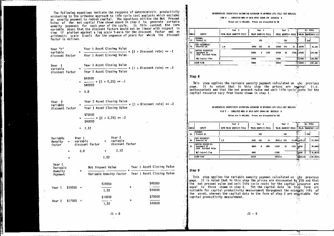
The following equations indicate the response of deterministic productivityaccounting to the orthodox approach to life cycle cost analysis which excludesan annuity payment to redeem capital. The equations utilize the Net PresentValue of the net capital flow shown above in step 2 to generate variableannuity payments for each year of the cycle. In this context the term
variable means that the discount factors would not be linear with respect totime If plotted against a log scale V—axis for the discount factor and an
arithmetic scale X—axis for the sequence of years for which the discountfactor is defined.
$40000- =—
$40000
$70000=
______
* [1 + 0,25] ** —2$40000
= 1,12
Variable Year 1 Year 2Annuityfactor
= variable +discount factor
variablediscount factor
= 0,8 + 1,12
BETEOMINISTIC ACCOUNTING EXTENSION TO 80100000 LIFt CYCLE COST ARALYSIU
STEP B CTRRECTED BOUE OF DATA ENTRY ROTaTOR FSR BUIIIIESS B
Values are in DOLLARS. Prices Ire discounted by 05
INDEX ENTITY
Year B
REYA YYLOE QOYNTITY PRICE
Year I
RALBE QUANTITY PRICE
Tear
VAIRE QOANTI
2 ALL YEARS
TV PRICE IYALOE IQOANIONIT ICC
- COST RESOURCES:Ni Material bi
CAPITAL REXTROCES:El Eqaipoeet HI
LESS Residual Value
BET Capital Ploa
iCYSR P100 -
1,8 8000 400
10000 B
20
1200
12140 570
17100 10
1:22 120140fff"
I
.
10000
18000
17000
30040
— 110,000
1192,160
Step 8
This step applies the variable annuity payment calculated on jhe previouspage. It is noted that in this step the prices are nijinal (i.e.undiscounted) and that the net present value and unit life cycleetosts for thecapital resource vary from those shown in step 1.
BETERRIBISTIC PRODUCTIVITY ACCOUNTIMO TO CNITOTROX LOPE CYCLE COST ANALYSIS
STCP B — CCOTRECTEB NOSE OP DATA ERTRY SHOWN POW ROSINESS B
Values are i' DOLLARS. Prices are discounted by 25%
Tear 0 Tear I Veer 2 ALL TEARS
IRDEI ENTITY RE0A VALUE QSORTITY PRICE VALUE QUANTITY PRICE VALUE RUANTITA PRICE IAUANIONIT LCC
REAETOUE:
01 Product HI 100 ISO 250
COST RESOURCES:RI BuLeriai HI 1,0 0400 400 16 8025,0 570 IU,08(ft420,b S7,7O24
CAPITAL RESOURCES:El Equipment HI 8000 B 1000 11210 10 1120 IØ200 70,0000
LESS Residoal Ralue
BET Capital Flow 0000 11200 76,0000
ICAS0 PLOW 04400 18225,6 14A25,Bl 113A,50241
Step 9
This step applies the variable annuity payment calculated on Qie previouspage. It is noted that in this step the prices are discounted byiS% and thatthe net present value and unit life cycle costs for the capital areequal to those shown in step 2. Yet the capital data in fore aresuitable for capital productivity measurement throughout the ecorlEllic life ofthe asset, whereas the capital data in the fore of step 2 are u4t&oitable forcapital productivity measurement.
REVENUE:81 Product HI 000 ISO 2501
Year °t°van ablediscount factor
Year t Asset Closing Value
Year 1
variable -discount factor
Year 1 Asset Closing Value
Year I Asset Closing Value
Year I Asset Closing Value
Year 2
variablediscount factor
= 0,8
Year 2 Asset Closing Value
Year 1 Asset Closing Value
* [1 + Discount rate] ** —t
* [1 + Discount rate] ** —i
* [1 + Discount rate] ** —2
1,92
Net Present Value Year t Asset Closing ValueYear tVariableAnnuityPayment
Year 1 $10000 =
Year 2 $17500 =
Variable Annuity Factor Year 1 Asset Closing Value
$19200 $40000
________
*1,92 $40000
$19200 $70000
1,92 $40000
________
*
J1—8 ji—g
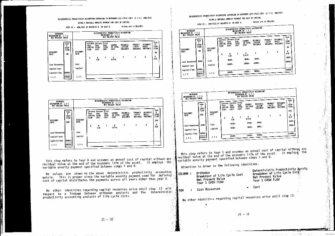
Current Current PriorTear Year Tear CHANGE RECONCIL PROUSCT RESOURCE 0
CAPITAL TOTAL TOTAL
FLOW COST COST
IN TOTALCOST
—lOTIONOARIANCE
—SHill PRICERARIANCE YARIANCE PLOW
OS
E F 0 0A 0 C
CoO EOF0O 0+0
DETERWINISYIC PROUACTINITY ACCOUNTIWO0000050WN OF I C C
NET PRESENT TALOE
Curront Current Prior Your
leer Yeor Year CHANGE RECONCIL PROUOCT RESOURCE
CAPITAL TOTAL TOTAL IN TOTAL —IATSON —lAITY PRICE CASH
PLOW COST COST COST 000IANCE YORIANCE OARIARCE FLOW
RETERRINSITIE PROUOCTITITT ACCEAJNIINO EOTENSIeI TO ORTNOUOX LIFE CYCLE COOT IL C C) ANALTOIS
00100 A YOWl WILE WNNAITY PAYMENT FUR COST OF CAPITAL
STEP 10 - ANALYSIS OF ROSINESS S IN YEAR N. Na)ues are in OOLLARS.
ORTOOROO
NREAEOOYW1 OF L C CNET PRESENT NOIRE
ORE0050)Wi OF L C CNET PRESENT OOLOE
Tear
CR50FLOW
OU
40000-
00000-
RETE001NISTIC PRWOCTIYITY ACCOUNTINGEOTENOIOW TO ORTWOUOA LIFE CYCLE COST )L C C) 000LYSSO
055WO A NORIORLE ARWOITY POAREWTFOR Cool OF CAPITOL
STEP IS — OCOLYSSS OF ROSINESS I IN YEAR I.NaiaeO are in 5011000-
RISCOUNYRATE
Coot
Capital
LCC
DISCOUNTRATE
Coot Re000r000
Capital Coot
Capital Flew
LEO
OUTNOUOO
0RE0000NN OP L C CRRE0000WW OF L C C
NET PRESENT NOLOEWET PRESENT AOLAE
Current Current PriorYear Year Year CHANGE RECONCIL
CAPITAL TOTAL TOTAL IN TOTAL —lOTION
PLOW COST COST COST YARIANCEI
IA
PROUACT RESOURCE
—INITY POICE
YARIONCE WORIAWCE
0 C Ii
COO E+F+O
0000—
UOOROUOO
ORE0000AN OF L C CRET PREOEWT AALOE
0
10000—
OUSO— 0000—
10000— 10000—
50000-
Year
COON
FLOW
210DISCOUNT DISCOUNT
HATE RATE- 050
A 0 C 0 0 F 0 N
CuD E+F+O 0+0
Cost Resources CosE
Capital Cost CapiEal
Capital Flow 40000—
_____________________________________________________________
LCC 40000— LCC
__________________________________________
This step refers to Year 0 and assumes an annual cost of capital without anyresidual value at the end of the economic life of the asset. It employs the
variable annuity payment specified between steps 7 and 8.
No values are shown in the above deterministic productivity accounting
matrix. This is proper since the variable annuity payment used for definiugcost of capital distributes the payments across all years other than year 0.
No other identities regarding capital resources arise until step 13 with
respect to a linkage between orthodox analysis and the deterministicproductivity accounting analysis of life cycle costs.
Ji — 10'
This step refers to Year 1 and assumes an annual cost of capital withood+ any
residual value at the end of the economic life of the asset. It emplofl the
variable annuity payment specified between steps 7 and 8.
Attention is drawn to the following identities:
COLUMN OrthodoxBreakdown of Life Cycle CostNet present ValueYear 1 CASH FLOW
ROW : Cost Resources
Oetermlnlstlc 4çcntg
Breakdown of Life Cycle Cost-Net present Value -
Year 1 CASH FLOW
= Cost
No otherregarding capital resources arise until step 13.
Ji — 11
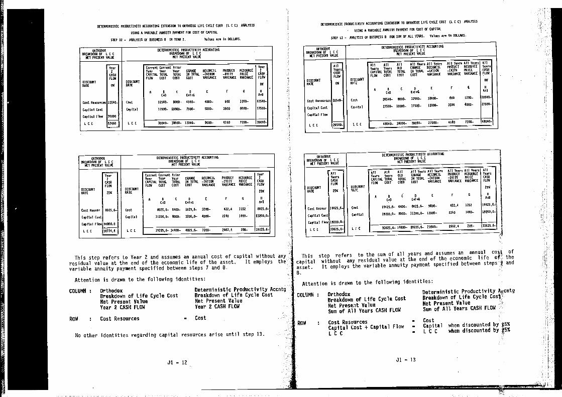
ENSTOE000
RREAE000NOF ICCNET PRESENT VALUE
DETERMINISTIC P000UCTI VITYIREAEDOI,00F ICC
NE! PRESENT VALUE
ACC01JNTING
DISCEWNYRAYE
Year2
CASh
FLOW
0%
DISCcOINTRATE
Current Current PrIorYear Year Tear CHANGE
CAPIYAL TOYAL YHYAL IN TOTALFLEW COSY COST COST
OECE4ICIL—IAYI01IAAUIANCE
PUEWOCT
—lAITYVARIANCE
RES01ITCEPRICEVARIANCE
Year2
CASH
FLOW
0%
-A N C S
CuD E+FoDE F U N
A+I
Cost Reuuurces 12540— Cost 12545— 0000— 4540— 4000— 660 1200— 12540—
Capital Cent Capital 17500— 10000— 7500— 5000— 3500 0005— 57100—
Capital Flow
C C
70000
57400 L C C 30040— 10000— 10040— 0000— 4160 7200— 30040—
OWTHWOO
IOtAKDO1,R1 OF L C CNET PRESENT VALAE
DETERMINISTIC P0000CTI VITOORE VE004,T4 OF L C C
NET PRESENT VOLOE
ACCOSNTINS
OISCWNTRATE
Year2
CASH
FLOW
250DISC060TRATE
Current Current PriorVeer Vear Year CHANGE
CAPITAL TOTAL TOTAL IN TOTALFLOW COST COST COST
RECONCIL—1011014VARIANCE
PREOUCT RESEAIRCE
—10110 PRICEVARIANCE VARIANCE
Year2
CASH
050
0 0 C 0
CuD E+F+O
E F 0 N
0+0
Cost Resour 0625,6— Coot 6025,0— 6400— 1625,0— 3200— 422.4 1102 6025,6—
Capital Coot Capital 11200,0— 8000— 3200,0— 4000— 2040 0400— 11200,0—
Capital Flow
ICC
44800,0
36774,4 L C C 01225,6— 14600— 4825,0— 7200— 2602,0 200-- 1R225,6—
This step refers to Year 2 and assumes an annual cost of capital withoutresidual value at the end of the economic life of the asset. It employsvariable annuity payment specified between steps 7 and 8.
Attention is drawn to the following identities:
AllYearsCASH
FLOW
RISCC*JNT
RATE 0%
DETERNINISTIC P0000CYI AlIT ACCEONTING ESTENSICN TO EMTiI0000 LIFE CYCLE COST (I C C) ANALYSIS
USING A VARIANLE ANNOITT PAYMENT FEW COST OF CAPITAL
STEP 02 — ANALVSIS OF NOSINESS N IN YEAR 2. Romeo are In DOLLARS.
REIERNINISTIC pREWACIIYITY ACCEOINTIMG EOTENSIGI TO EWT00600 LIFE CYCLE COST )L C C) ANALYSIS
-ASING A RAOIARLE ANNUITY PAYRE6T PENS COST OF CAPITAL
STEP 13 — ANALYSIS OF ROSINESS N FEll 506 OF ALL TEARS. Names are lo ROLLNSO5.
EWT5000S — DETERMINISTIC PRSI1OCTIVITY ACCEAJRYINO
RRE00000IM or L C C ORE0000I6O OF L C C
NET PRESENT VALOENET PRESENT VALOE
Coot Resources 20540—
Capital Coot
Capital FToa
LCC 20540—
All All All All Years All Years Oil Years AlT Years All
Tears Years OLD CHANGE RECEUICIL P0000CT RESEOIOCE Years
CAPITAL TOTAL YOTAL IN TOTAL —IATIENI —lAiTY PRICE CASH
FLOW COST COST COST VARIANCE VARIANCE VARIANCE FLEW
DO SC. WIT
HAIc0%
A R C U F F 0 0
CoO E+F+OAul
20540— 0600— 02540— 12001— 660 1200— 20540—
Camital 27500— 10000— 57500— 15000— 3500 6000— 27500—
C C 40040— 16000— 30040— 27000— 4160 1200— 40060—
-
anythe
ROW
COLUMN : OrthodoxBreakdown of Life Cycle CostNet Present ValueYear 2 CASH FLOW
Cost Resources — Cost
Deterministic Productivity AccntgBreakdown of Life Cycle CostNet Present ValueYear 2 CASH FLOW
This step refers to the sum of all years and assumes an annual cos% of
capital without any residual value at the end of the economic life of the
asset. It employs the variable annuity payment specified between steps and
8.
Attention is drawn to the following identities:
No other identities regarding capital resources arise until step 13.
Ji — 12
COLUMN OrthodoxBreakdown of Life Cycle CostNet Preseat ValueSum of All Years CASH FLOW
ROW : Cost ResourcesCapital Cost + Capital FlowLCC
Ji — 13
Deterministic ProductivityBreakdown of Life Cycle CosçNet Present Value -
Sum of All Years CASH FLOW -
— Cost— Capital when discounted by 45%— L C C when discounted by
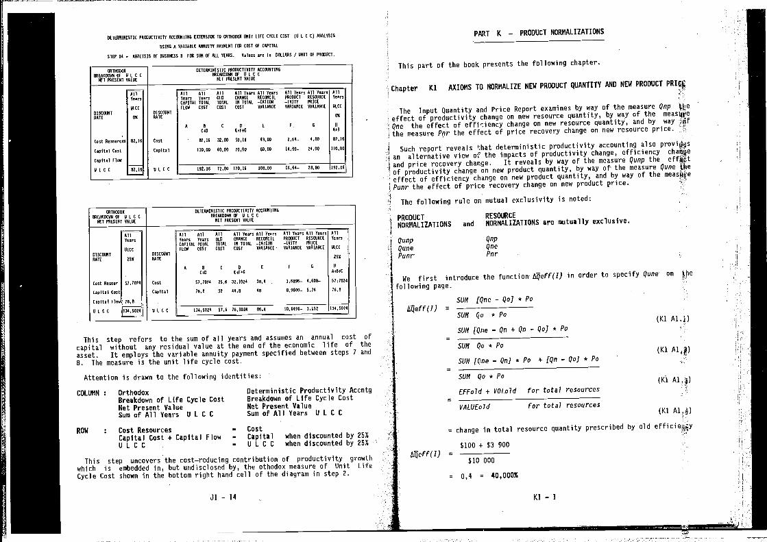
DETERMINISTIC PNODUCTIAITT ACCWNTIAG EXTENSIOW 10 ENTITWAA UNIT LIFE CYCLE COST (U L C C( ANALYSIS
RUING A TAAIAAL( ANNUITY PATMENT PEA CURT UP CAPITAL
STEP 14 — APENLYSIS UP RASINESS N PEA SAN UP ALL TEARS. Tallies are In DOLLARS / UNIT UP PRODUCT.
EATNODOG
NNEA000AN UP 0 1 C CNET PRESENT TAINt
DITERNINISTIC PNOUUCTIAITT ACCOUNTINGNNEAUOUENI OP U L C C
NET PRESENT AALUE
DISCOUNTRAID
Cost Neanarcen
Capital Cast
Capital Flew
N L C C
AllTears
61CC
0%
NO.16
R2,IN
OISCODNTNATE
CnnE
Capital
N I C C
All All All All Yearn All Years All Yearn All TearsYearn Tears ALl CAANRE NECONCIL PRODUCT NESOURCE
CAPITAL TOTAL TOTAL IN TOTAL —IATIEN1 —lAITY PRICE
PLOW COST COST COST AANIANCE TATIANCE AANIANCE
A I C 2 E P 0
Call EaPAG
NO.10 32,00 50,16 lOUT 2,64— 6,NO
11000 48,00 70,00 ROOT 14,00— 04,00
AllYears
ULCC
OS
A
YeN
60,10
hOOT
190,10 70,00 100,10 IAN,00 16,60— ON,NA INO,16
ODTNODOO
NNEACOORN UP A L C CRET PRESENT TALUE
DETENNINISTIC PN000CTIAITT ACCOUNTINGNNEAKOOAN UP A L C C
NET PNERENT AALOE
OISCEAINTTOTE
ConS Nennar
Capital Cost
Capital Ploe
N I C C
AllTears
NLCC
250
57,7604
76,1
I.34,5N04
DISCOUNT
NATE
Cost
Capital
N L C C
All All All All Tears All Years All Tears All TearsTears Tears OLD CNANGE DECORCIL PRODUCT NOSOROCE
CAPITAL TOTAL TOTAL IA TOTAL —IAIIOR —lAITY PRICE
PLOW CURT COST COST AANIARCE AANIANCO AANIANCE
A I C 0 E P 0
CeO (eP+O
57,7026 05,6 32,1024 38,4 l,NAAO— A,AON—
PRO TO 44,1 46 N,AATU— 1.76
134,0004 hR 76,9024 86.6 10,6416— 1,112
AllTears
ULCC
210
A
A+N+C
RT;7020
IR.N
134,1004
PART K — PRODUCT NORMALIZATIONS
This part of the book presents the following chapter.
Chapter Ki AXIOMS TO NORMALIZE NEW PRODUCT QUANTITY AND NEW PRODUCT PRICE
The Input Quantity and Price Report examines by way of the measure Qnp the
effect of productivity change on new resource quantity, by way of theQne the effect of effiiency change on new resource quantity, and by way Ifthe measure Pnr the effect of price recovery change on new resource price.
Such report reveals that deterministic productivity accounting alsoan alternative view of the impacts of productivity change, efficiencyand price recovery change. It reveals by way of the measure Qunp the effjttof productivity change on new product quantity, by way of the measure Qune floe
i effect of efficiency change on new product quantity, and by way of thePunr the effect of price recovery change on new product price.
The following rule on mutual exclusivity is noted:
Qunp Qnp
Qune Qne
Punr Pnr
We first introduce the function in order to specify Qune on the
following page.
SUM (Qne — Qo] * Po
SUM Qo * Po (Ki Al.!)
J1—14 1(1—1
PRODUCTMORMALIZATIOMS
RESOURCE
and MORMALIZATIOMS are mutually exclusive.
This step refers to the sum of all years and assumes an annual cost ofcapital without any residual value at the end of the economic life of the
asset. It employs the variable annuity payment specified between steps 7 and8. The measure is the unit life cycle cost.
Attention is drawn to the following identities:
COLUMN : OrthodoxBreakdown of Life Cycle CostNet Present ValueSum of All Years U L C C
ROW : Cost ResourcesCapital Cost + Capital Flow —
ULCC —
Deterministic Productivity AccntgBreakdown of Life Cycle CostMet Present ValueSum of All Years U L C C
CostCapitalULCC
when discounted by 25%when discounted by 25%
This step uncovers the cost—reducing contribution of productivity growth
which is embedded in, but undisclosed by, the othodox measure of Unit LifeCycle Cost shown in the bottom right hand cell of the diagram in step 2.
SUM fQne — Qn + Qn — QoJ * Po
SUM Qo * Po(Ki Al7?)
SUM fone—QnJ*Po +(Qn_QoJ*PO
SUM Qo*Po (K1 Al.3)EFFo1d + VOLold for total resources
VALUEo7d for total resources(Ki A1,4)
= change in total resource quantity prescribed by old
$100 + $3 900=
$10 000
= 0,4 = 40,000%
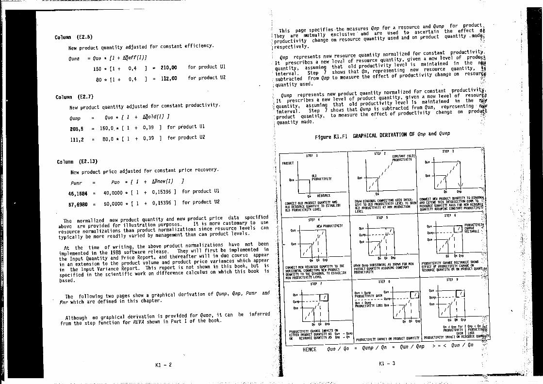
Column (E2.5}
New product quantity adjusted for constant efficiency.
Qune = Quo * (1 +
150 * [1 ÷ 0,4 ] = 210,00 for product Ui
80 * [1 + 0,4 ] = 112,00 for product U2
Column (E2.7}
New product quantity adjusted for constant productivity.
Qunp = Quo * + 14o7d(I) ]
208,5 = 150,0 * [ 1 + 0,39 ] for product Ui
111,2 = 80,0 * [ 1 + 0,39 ] for product U2
Column (E2.13)
New product price adjusted for constant price recovery.
Punr = Puo * (1 + ls2new(I)
46,1584 = 40,0000 * [ 1 + 0,15396 1 for product Ui
51,6980 = 50,0000 * 1 1 + 0,15396 ] for product U2
The normalized new product quantity and new product price data specified
above are provided for illustration purposes. It is more customary to use
resource normalizations than product normalizations since resource levels can
typically be more readily varied by management than can product levels.
At the time of writing, the above product normalizations have not been
implemented in the 1988 software release. They will first be implemented in
the Input Quantity and Price Report, and thereafter will in due course appear
in an extension to the product volume and product price variances which appear
in the Input Variance Report. This report is not shown in this book, but is
specified in the scientific work on difference calculus on which this book is
based.
The following two pages show a graphical derivation of Qunp, Qnp, Punr and
Pnr which are defined in this chapter.
Although no graphical derivation is provided for Qune, it can be inferred
from the step function for REVA shown in Part I of the book.
KI — 2
• This page specifies'the measures Qnp for a resource and Qunp for product,
They are mutually exclusive and are used to ascertain the effect
productivity change on resource quantity used and on product quantity
Qnp represents new resource quantity normalized for constant
it prescribes a new level of resource quantity, given a new level of produfl
quantity, assuming that old productivity level is maintained in the
interval. Step 7 shows that Qn, representing new resource quantity,
subtracted from Qnp to measure the effect of productivity change on
quantity used.
Qunp represents new product quantity normalized for constant productivity.
it prescribes a new level of product quantity, given a new level of resourO
quantity, assuming that old productivity level is maintained in the nui
interval. Step 7 shows that Qunp is subtracted from Qun, representing nn
product quantity, to measure the effect of productivity change on
made.
Figure K1.F1 GRAPHICAL DERIVATION OF Qnp and Qunp
STEPZS1EPXCONSTANT (OLD)
:E"L,Qo RESORDCE
0' 0'
CONNECT OLD PROROCT Q0ANTFn ANDDRAW DIASEWAL CONNECTION AXIS INTER—
CONNECT NEW PROROCT Q0ANTITY TO DIA0m4AL
I OLD REDORDCE QOONTITY TO ESTABLISHCEPT TO OLE POOROCTI WIlT LEVEL TO SOON
AND EXTEND This INTERSECTION SOON TO
OLD PRcDOCT1YITY LEVELALE pOOROCTI VIII AT ANY
RESORRCE QUANTITY AXIS FOR DEW REDCURCL I
LEVELQUANTITY 0050NINO CONSTANT PRORUCTI Vii!
sTEP 4STEP S
STEP 6 1
:: EENPOOROCTIVITY
Qo 0, Q'o Qo QnQo nQop
CONNECT DEN RESORRCE QUANTITY TO rOEDRAW Quop HORIZONTAL AS SHOWN FOR MEN
PROROCTINIIY CAANGE RECTANGLE SHOWS
HORIZONTAL CONNECTING MEN PROROCTPHORUCT QUANTITY ASSONINS CONSTANT
EFFECT OF PRORUCTINITY CHANGE OR
QUANIITT TO THE DIAGONAL TO ESTASLTSS PVOROCTSYITTSESOROCE QUANTITY OR OR PRORACT
DEN PROROCTIVITT LEVEL --
STEP 1sTEP 0
STEP S
Qo
Qo Qo Qo Qop
POOROCTIVITT CONNSE IMPACTS ON
Q, < Qop For Qop C I, W
EIThER PRORUCT QSHNTITT AS Qo' — QuopPOOROCTIVITY
OR NESOROCE OOANTITT AS Qop — Qo
GAIN LOSS
PROROCTENIIY IMPACT ON POORACT QOANTIITPRCOOCIIYITY IMPACT OR RE OROCE QUANUIY
HENCE Quo/Qo = Qunp/Qn = Qun/Qnp >=< Qun/Qn
K1—3
I
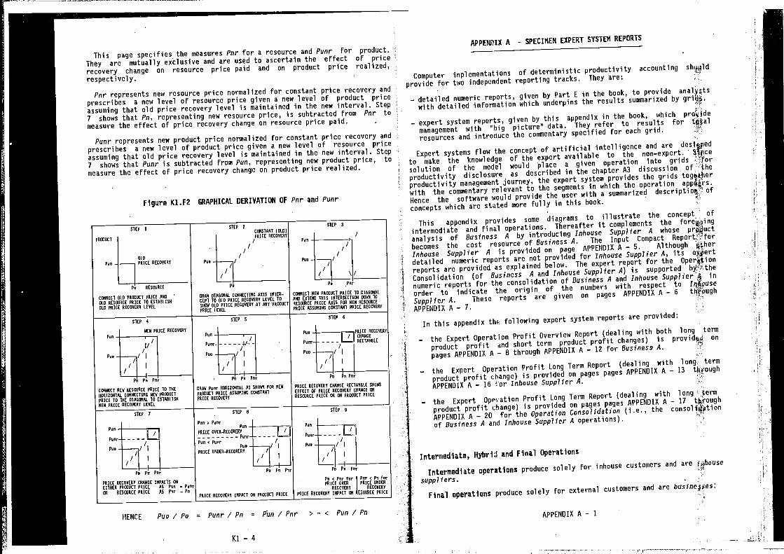
This page specifies the measures Pnr for a resource and Punr for product.
They are mutually exclusive and are used to ascertain the effect of price
recovery change on resource price paid and on product price realized,
respectively.
Pnr represents new resource price normalized for constant price recovery andprescribes a new level of resource price given a new level of product price
assuming that old price recovery level is maintained in the new interval . Step
7 shows that Pn, representing new resource price, is subtracted from Pnr to
measure the effect of price recovery change on resource price paid.
Punr represents new product price normalized for constant price recovery andprescribes a new level of product price given a new level of resource price
assuming that old price recovery level is maintained in the new interval. Step7 shows that Punr is subtracted from Pun, representing new product price, to
measure the effect of price recovery change on product price realized.
Figure K1.F2 GRAPHICAL DERIVATION OF Pnr and Punr
STEP I STEP I STEP 3
APPENDIX A - SPECIMEN EXPERT SYSTEM REPORTS
computer inplementations of deterministic productivity accounting shvgld
provide for two independent reporting tracks. They are:
— detailed numeric reports, given by Part E in the book, to provide
with detailed information which underpins the results summarized by griA$.
— expert system reports, given by this appendix in the book, which proiiide
management with "big picture" data. They refer to results for tflalresources and introduce the commentary specified for each grid.
Expert systems flow the concept of artificial intelligence and are deslgjied
to make the knowledge of the expert available to the non—expert. Sfvce
solution of the model would place a given operation into grids :for
productivity disclosure as described in the chapter A3 discussion of the
productivity management journey, the expert system provides the gridsto the segments in which the operation
Hence the software would provide the user with a summarized of
concepts which are stated more fully in this book.
This appendix provides some diagrams to illustrate the concept of
intermediate and final operations. Thereafter it complements the
analysis of Business A by introducing Inhouse Supplier A whose prpduct
becomes the cost resource of Business A. The Input compact
Inhouse Supplier A is provided on page APPENDIX A — 5. Although $her
detailed numeric reports are not provided for Inhouse supplier A, its
reports are provided as explained below. The expert report for the Operjtion
consolidation (of Business A and Inhouse Supplier A) is supported
numeric reports for the consolidation of Business A and Inhouse Supplier in
order to indicate the origin of the numbers with respect to
supplier A. These reports are given on pages APPENDIX A — 6
APPENDIX A - 7.
— the Expert Operation Profit Overview Report (dealing with both long term
product profit and short term product profit changes) is providpd on
pages APPENDIX A - B through APPENDIX A - 12 for Business A.
— the Expert Operation Profit Long Term Report (dealing with long- term
product profit change) is provided on pages pages APPENDIX A — 13
APPENDIX A - Cor Inhouse Supplier A.
— the Expert Oprvation Profit Long Term Report (dealing with long term
product profit change) is provided on pages pages APPENDIX A — 17
APPENDIX A — 20 for the Operation Consolidation (i.e., theof Business A and Inhouse Supplier A operations).
Intermediate, Hybrid and Final Operations
Intermediate operations produce solely for inhouse customers and are iahouse
suppliers.
Final operations produce solely for external customers and are
APPENDIX A - I
CONSTANT (OLD)PRICE RECAREAR
I/
I I
DRAW DIAGONAL CONNECTING AXIS INTER-CEPT TA OLD PRICE RECORERT LEREL TOSWAN OLD PRICE RECORERO AT ANT PRONACT
PRICE LEREL
STEP S
:4 - - -
Pa Pn Pnr
ROAN Punr AOUIZONTAL AS SHOW Fm NEWpR000CT PRICE ASSONING CONSTANTPRICE RECORERA
Pun //
Pun /
II \/Pa Par
CONNECT NEW PRONACT PRICE TO DIAGONALAND EXTEND TRIS INTERAECTION DOW TARESOURCE PRICE WAIT FON NEW RESOURCEPRICE ADAANINO CONSTANT PRICE RECAVERA
STEP N
Pan PRICE REC00000
I CNANOE
Puar— — — —
NECTRRDLE
Pua / I
/1/
Pa In Pnr
PRICE OECOAEOT CRANOE RECTANGLE SROATEFFECT OF PRICE RECAAERT CHANGE ONRESOURCE PRICE ON ON PROUACT PRICE
PRONACT
OLD
Pun PRICE RECDRERT
Pa REIOUDCE
CONNECT OLD FRONOCT PRICE ANDOLD RESOURCE PRICE 10 ESTANLIINDLD PNICE RECORERT LEVEL
SIEP 4
NEW PRICE RECDRERT
1/iPa Pn Pnr
CONNECT NEW RESOURCE PRICE TO IREHONIZONTAL CONRECTINO NEW POOUACTPRICE TO THE DIAOONAL 10 ESIADLISNNEW PRICE RECARERA LEREL
STEP 7
Pun
I /Panr — — — —,
Pun / I
/ I
Pa Pn Pnr
PRICE RECARERA COUNAE IMPACTS ONEIThER PROUOCT PRICE AX Pun — Punr
CO RESOURCE PRICE AS Par — Pn
4
In this appendix the following expert system reports are provided:
SIEP NSTEP
Pun PunrPun DPRICE RRER-OECDYEOVPuar
Pun A PuarPun
PRICE ANDER—RECARERA
Pa Pa Par
Pun
rmlI / i
Pa Pa
Pa < Par Far Par < Pa farPRICE ORER PRICE ORDER
RECOTERO RECATERA
PRICE RECORERO IMPACT ON PROUOCT PRICE PRICE RECORERA IMPACT ON ESOURCE PAICD
HENCE Puo/Po = Punr/Pn = Pbn/Pnr >=< Pun/Pn
Kl — 4
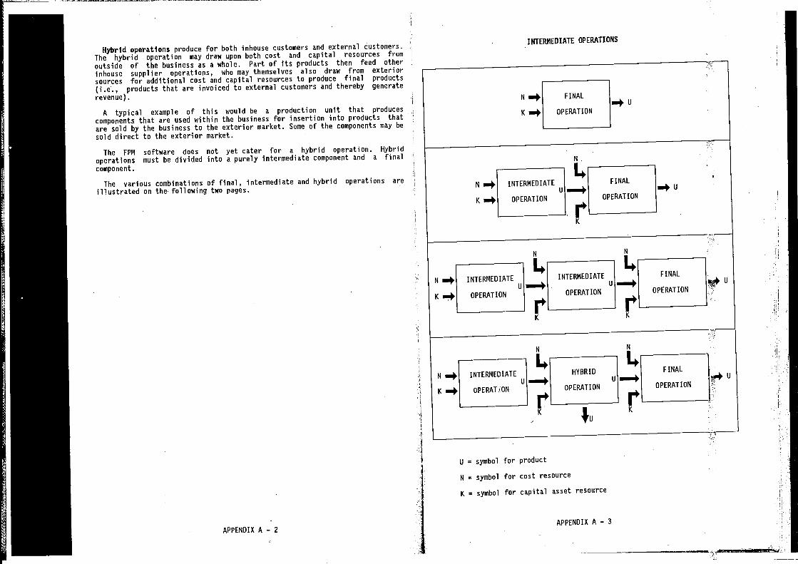
Hybrid operations produce for both inhouse customers and external customers.The hybrid operation may draw upon both cost and capital resources from
outside of the business as a whole. Part of Its products then feed otherinhouse supplier operations, who may themselves also draw from exteriorsources for additional cost and capital resources to produce final products
(i.e., products that are invoiced to external customers and thereby generate
revenue).
A typical example of this would be a production unit that produces
components that are used within the business for insertion into products thatare sold by the business to the exterior market. Some of the components may besold direct to the exterior market.
The FPM software does not yet cater for a hybrid operation. Hybrid
operations must be divided into a purely intermediate component and a finalcomponent.
The various combinations of final, intermediate and hybrid operations are
illustrated on the following two pages.
APPENDIX A — 2
U = symbol for product
N = symbol for cost resource
K = symbol for capital asset resource
APPENDIX A — 3
INTERMEDIATE OPERATIONS
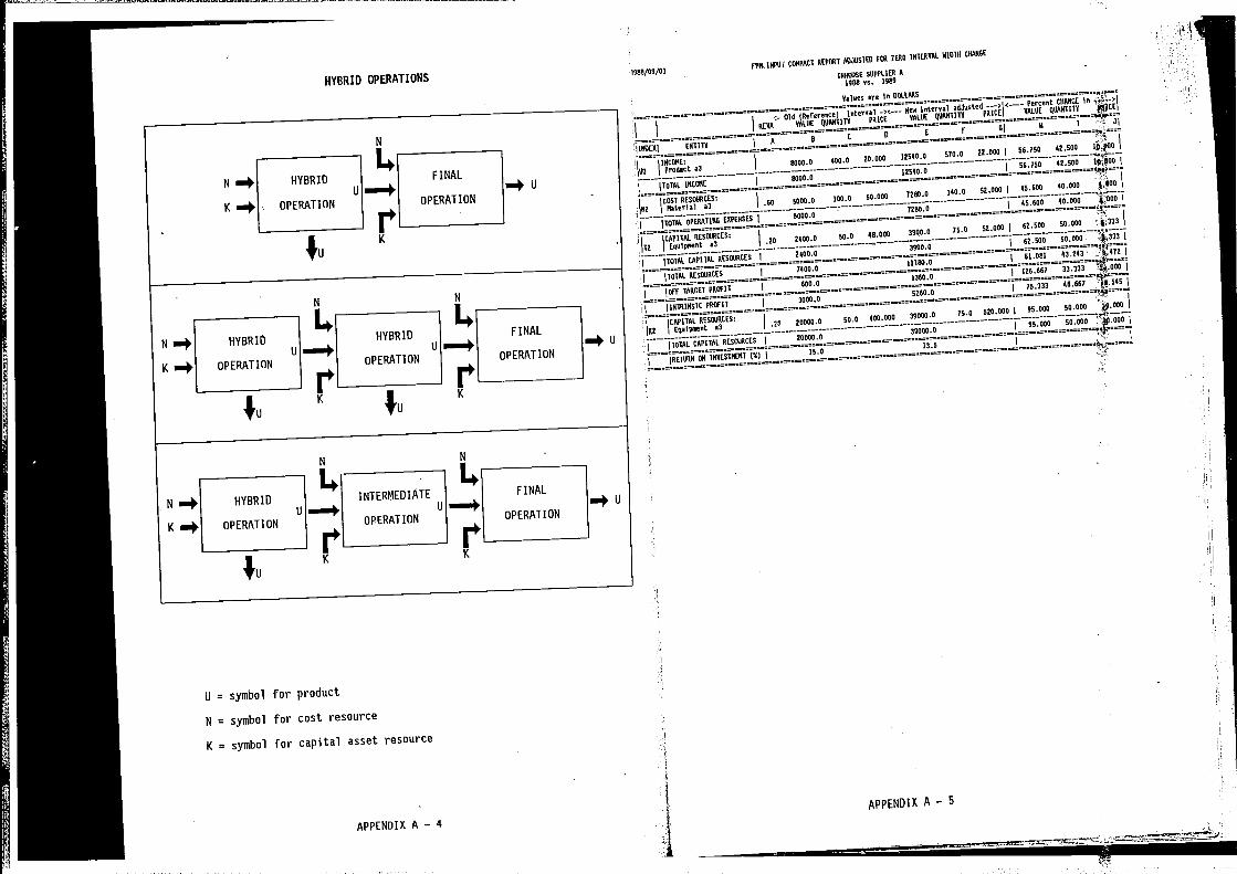
HYBRID OPERATIONS1900/00/01
PPM. INPUT CEIIPACT REPEOTADJUSTER PEI1 ZERO INTERVAL
WIDTH CHANGE
INVERSE SUPPLIER AIRAN vs. 1909
VeTOeR eve In DOLLARS
INREXIENTITY
Old (Reference)Interval —>c——— New InteresT
adjosted ———> C———— PRrCRIIECHANGE In
REVO VALUE QUANTITY PRICE VALUE QIJANTIB PRICE VALUE QUANTITY $JCE
A S C E E F El A
INCENE:
Y
03 PredatE w3
TRIAL INCCI4E
0000.9 4RR.0 20.000 12540.0 570.0 22.000 SR.75R 42.500 11,200
00000
I
.
COST IIE0000CES:
02 Naterlal a3 .00 5000.0 150.0 50.000 12R0.I 100.0 52.000 45.000 4R.E00
I -- TOTALETPE9GES - --
720045.600 40.000 ftoo I
TO Equipment s3 .20 2400.0 50.0 40.000 3500.0 15.0 52.000 62.500 50.000
.
30052.500 50:000 j333
;rTr;RorflI1NTOINSIC PROFIT
3000 05200 0
75 333 40 607 545
E2 EquIpment o3 .20 20000.0 50.0 400.000 39000.0 75.0 520.000 95.000 50.000 20.000
TOTAL CAPITAL RESEORCER20000.0
30000.0 j 95.000 50.000 'hOOD)
N = symbol for cost resource
APPENDIX A — 4
IAPPENDIX A — 5
-
NN
INTERNEDIATEFINAL
r ERATION
U
OPERATIONOP
4 KK
U = symbol for product
K = symbol for capital asset resource
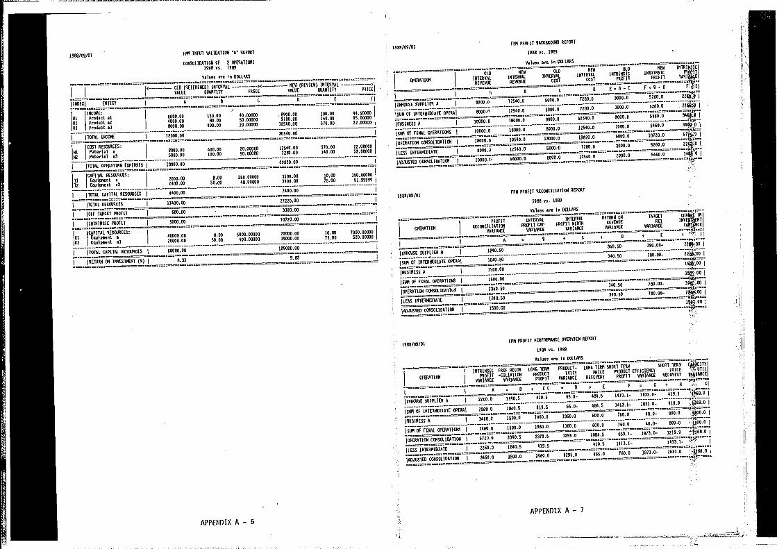
1988/09/01FPN INPUT VALIDATION 'U' REPORT
CONSOLIDAIION OF 2 OPERATIONS
1989 vs. 1909
Values are in DOLLARS
(iNDEX) ENTITY A I C D
INCOME:
UI Product ci 0000.00 100.00 40.00000 0000.00
02 ProducE a2 4000.00 90.00 50.00000 1100.00
03 Product a3 8000.00 400.00 20.00000 12540.00
INCOME 18000.00 30540.00
COST RESOURCES:
NI Maoerlal a 9000.00 400.00 00.00000 12540.00 570.00 22.00000
82 Material a3 5000.00 100.00 50.00000 7200.00 140.00 02.00000
IITOTUL OPERATING EXPENSES I
13000.0019820.00
CAPITAL RESOURCES:
TI Equipment a 0000.00 8.00 050.00000 3500.00 10.00 300.00000
TO Equipment a3 - 0000.00 50.00 40.00000 3900.00 70.00 01.09900
I)TOTUL CAPITAL RESOURCES I
4400.00 7400.00
ITOTAL RESOURCES I17400.00 27020.00
I10FF TARGET PROFIT I
600.00 3320.00 = -—
141018010 PROFIT 5000.00 10720.00
CAPITAL RESOURCES:
01 Eqalpoent a 40000.00 0.00 5000.00000 70000.00
02 Equipment u3 00000.00 50.00 400.00000 30000.00
I110101. CAPIIAL RESEOJRCEI 00000.00 109000.00
I044 INVESTMENT (5) 8.33 9.03
APPENDIX A — 6
1900/09/UI
0988/09/01
MEW OLD NEW OLD MEW 091009010
OLD (REFERENCE) INTERNALNEW (REVIEW) INTERVAL
UPERATIGII INTERVAL INTERVAL IMIERVUL INTERVAL 18I00051C INTRINSIC PR'#IT
VALUE QUANTITY PRICE VALUE QUANTITY PRICE1=_======?
FRONT PROFIT
i 1
0 EAC 7:8-0
(148GIISE SUPPLIER A I6000.0 12540.0 5000.0 700.0 3000.0 5200.0 2268.0 I
0:90
7280 3000 sooo
570.00 22.00000'
SUM OF FINAL OPERATIONS I00000.0 18000.0 8080.0 12540.0 2000.0 0400.0
(OPERATION CONSOLIDATION )
18000.0 30540.0 13000.0 19020.0 0000.0 10700.0 I
(LESS INTERMEDIATE = (8000.0 12540.0 5000.0 7280.0 3000.0 0080.0 I
(AUJUUIED CONSULIOUTIEM )100000 08000.0 -- 8000.0 - 12540.0 2000.0 5060.0 3440
1008/09/007PM PROFIT RECDNCILIATOE*I REPORT --
0988 vu. 0989
Values are in OOLL005
PROFIT INTERVAL INTERVAL UET000 UN TARGET 184 19
00 00 7000 00000OPERATION
RECONCILIATION PROFIT GAP PROFIT 90010 REVENUE RVI INVES — NT
75:02
VARIANCE VARIANCE VARIANCE VARIANCE VARIANCE 0*T4CE
L0 +
(INV005E SUPPLIER U I0800.50
340.50 780.00- I
(GUM OF INTERMEDIATE UPERU(02.00.50
340.50 780.00- 22goo I
(BUSINESS 8 I1500.00
10MO0 I
(000 OF FINAL OPERATIONS I0500.00
I
(070001188 CONSOLIDATION I= 3340.50
-- 340.00 780.00- I
(LE TEOIIEOIA'IE 1340.00340.50 .00
—
FF8 PROFIT BACKGROUND REPORT
198045. 0189
Values are In UOLLMS
FF8 PROFIT PERFUR1'GINCE OVERVIEN REPORT
1988 vs. 1089
APPENDIX:-7 —fl
.
!
0=8+ CC 0 + E P = 0 v
io.5 410.5;5.o_SOO.51413.i:10330_4149W4°I
2200,0 1840.5 419.5 00.0— 480.5 1413.1— 0833.0- 419.9 'fl6U.Q(
H
(00807 INTERMEDIATE
(BUSINESS A 3460.C 1000.0 1900.0 1360.0 600.0 700.0 40.0— 800.0 I
UP FINAL OPERATIONS I 3460.0 1500.0 0080.0 1300.0 600.0 760.0 40.0- 800.0
(SUN
(OPERATION CONSOLIDATION (5724.0 3340.0 2379.5 0290.0 0086.5 053.1- 1873.0- 1210.9 24100.0
1[i[cINT500EO10T
1
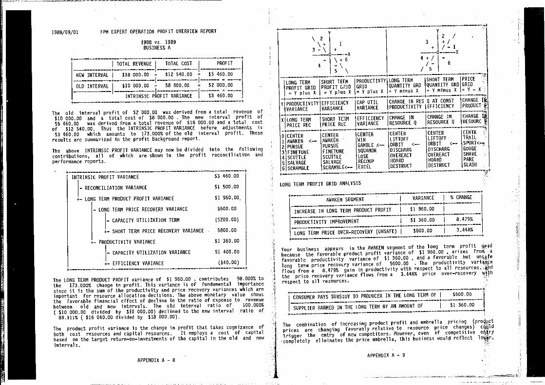
The old interval profit of $2 000.00 was derived from a total revenue of$10 000.00 and a total cost of $8 000.00 . The new interval profit of$5 460.00 was derived from a total revenue of $18 000.00 and a total cost
of $12 540.00. Thus the INTRINSIC PROFIT VARIANCE before adjustments is$3 460.00 which amounts to 173.000% of the old interval profit. These
results are summarized in the profit background report.
The above INTRINSIC PROFIT VARIANCE may now be dividedcontributions, all of which are shown in the profitperformance reports.
The LONG TERM PRODUCT PROFIT variance of $1 960.00 , contributes 98.000% tothe 173.000% change in profit. This variance is of fundamental importancesince it is the sum of the productivity and price recovery variances which areimportant for resource allocation decisions. The above monetary value shows
the favorable financial effect of decline in the ratio of expense to revenue
between old and new intervals. The old interval ratio of 100.000%
($10 000.00 divided by $10 000.00) declined to the new interval ratio of89.111% ( $16 040.00 divided by $18 000.00).
The product profit variance is the change in profit that takes cognizance ofboth cost resources and capital resources. It employs a cost of capitalbased on the target return—on—investments of the capital in the old and new
intervals.
\2 2/\+ 1
3 -s-/
3—\ ++ I—i
0 X 0 X
— \+6 4+! —
4 —\ /— 6
5 \ /5TERM SHORT TEEM PROOUCTIVTY LONG TERM SHORT TERM PRICE
GRID PROFIT G11D GRID QUANTITY GRD QUANTITY GRD GRID
=VplusX =YplusX =YplusX =YminusX =YminusX =Y-X+ + +
PRDDUCTIVITV EFFICIENCY CAP UTIL CHANGE IN RES Q AT CONST CHANGE
VARIANCE VARIANCE PRODUCTIVITY jEFFICIENCY
- .———— + +
TERM SHORT T[RM EFFICIENCY CHANGE IN CHANGE IN CHANGE
REC PRICE REC VARIANCE RESOURCE Q RESOURCE Q RESOURC
-+. + + -4
CENTER CENTER CENTER CENTER CENTR
<—— AWAKEN WIN LIFTOFF LIFTOFF TRAILORBIT c——
PURSUE
FINETUNESCUTTLESALVAGESCRAMBLEC——
GAMBLE c——
SQUANDR
LOSERECOUP
EXCEL
ORBITDISCHARG DISCHARG
OVEREACT OVEREACT
HOARD HOARD
DESTRUCT DESTRUCT
GOUGE
SHAVEPARE
SLASH
-
I N LONG TERM PRODUCT
F- +
PROFIT I$1 960.00
I8.479%
-PRODUCTIVITY IMPROVEMENT
LONG TERN PRICE OVCR—RECOVERY (UNSAFE)
Your business appears in the AWAKEN segment of the long term profitbecause the favorable product profit variance of $1 960.00 , arises fronj a
favorable productivity variance of $1 360.00 , and a favorable but
long term price recovery variance of $600.00 . The productivityflows from a B.479% gain in productivity with respect to all resources,the price recovery variance flows from a 3.448% price over—recovery with
respect to all resources.
++
CONSUMER PAYS SUBSIDY TO PRODUCER IN THE LONG TERM OF I$600.00
+
SUPPLIER HARMED IN THE LONG TERM BY AN AMOUNT OF I$1 360.00
+-t
The combination of increasing product profit and umbrella pricingprices are changing favorably relative to resource price changes)
trigger the entry of new competitors. However, even if competitive
-completely eliminates the price umbrella, this business would reflect
APPENDIX A — 9
1988/09/01 FPM EXPERT OPERATION PROFIT OVERVIEW REPORT
1988 vs. 1989BUSINESS A
NEW INTERVAL $18 000.00 — $12 540.00 = $5 460.00+ I I
OLD INTERVAL $10 000.00 — $8 000.00 = $2 000.00
INTRINSIC P/OFIT VARIANCE $3 460.00
into the followingreconciliation and
INTRINSIC PROFIT VARIANCE $3 460.00
RECONCILIATION VARIANCE $1 500.00
+— LONG TERM PRODUCT PROFIT VARIANCE $1 960.00
— LONG TERM PRICE RECOVERY VARIANCE $600.00
CAPACITY UTILIZATION TERM ($200.00)
+— SHORT TERM PRICE RECOVERY VARIANCE $800.00
+— PRODUCTIVITY VARIANCE $1 360.00
CAPACITY UTILIZATION VARIANCE $1 400.00
+— EFFICIENCY VARIANCE ($40.00)
LONG TERM PROFIT GRID ANALYSIS
$600.00 3.448%
APPENDIX A — 8
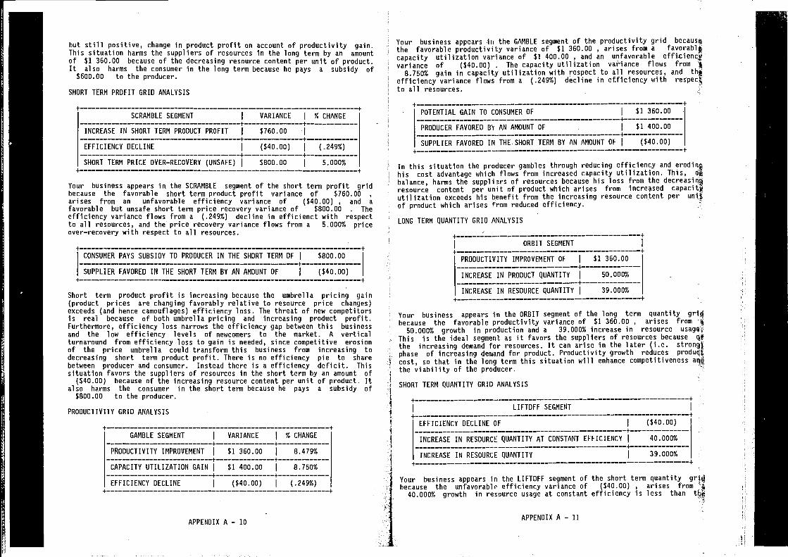
but still positive, change in product profit on account of productivity gain.This situation harms the suppliers of resources in the long term by an amountof $1 360.00 because of the decreasing resource content per unit of product.It also harms the consumer in the long term because he pays a subsidy of
$600.00 to the producer.
SHORT TERM PROFIT GRID ANALYSIS
Your business appears in. the SCRAMBLE segment of the short term profit gridbecause the favorable short term product profit variance of $760.00arises from an unfavorable efficiency variance of ($40.00) , and a
favorable but unsafe short term price recovery variance of $800.00 . Theefficiency variance flows from a (.249%) decline in efficienct with respectto all resources, and the price recovery variance flows from a 5.000% priceover—recovery with respect to all resources.
+ +
CONSUMER PAYS SUBSIDY TO PRODUCER IN THE SHORT TERM OF $800.00+
SUPPLIER FAVORED IN THE SHORT TERM BY AN AMOUNT OF ($40.00)
Short term product profit is increasing because the umbrella pricing gain(product prices are changing favorably relative to resource price changes)exceeds (and hence camouflages) efficiency loss. The threat of new competitorsis real because of both umbrella pricing and increasing product profit.Furthermore, efficiency loss narrows the efficiency gap between this businessand the low efficiency levels of newcomers to the market. A verticalturnaround from efficiency loss to gain is needed, since competitive erosionof the price umbrella could transform this business from increasing todecreasing short term product profit. There is no efficiency pie to sharebetween producer and consumer. Instead there is a efficiency deficit. Thissituation favors the suppliers of resources in the short term by an amount of
($40.00) because of the increasing resource content per unit of product. Italso harms the consumer in the short term because he pays a subsidy of
$800.00 to the producer.
PRODUCTIVITY GRID ANALYSIS
GAMBLE SEGMENT VARIANCE % CHANGE
PRODUCTIVITY IMPROVEMENT $1 360.00 8.479%
CAPACITY UTILIZATION GAIN $1 400.00 8.750%
EFFICIENCY DECLINE ($40.00) (.249%)
Your business appears the GAMBLE segment of the productivity grid becausethe favorable productivity variance of $1 36O.D0 , arises from a favorablicapacity utilization variance of $1 400.00 , and an unfavorable efficiencjvariance of ($40.00) . The capacity utilization vatiance flows from
8.750% gain in capacity utilization with respect to all resources, and thpefficiency variance flows from a (.249%) decline in efficiency with respectto all resources.
+ ÷
POTENTIAL GAIN TO CONSUMER OF $1 360.00+
PRODUCER FAVORED BY AN AMOUNT OF. I
$1 400.00+
SUPPLIER FAVORED IN THE SHORT TERM BY AN AMOUNT OF j($40.00)
In this situation the producer gambles through reducing efficiency and erodinghis cost advantage which flows from increased capacity utilization. This,balance, harms the supplisrs of resources because his loss from theresource content per unit of product which arises from increased capacitijutilization exceeds his benefit from the increasing resource content per unitof product which arises from reduced efficiency.
LONG TERM QUANTITY GRID ANALYSIS
Your business appears in the ORBIT segment of the long term quantity grI4because the favorable productivity variance of $1 360.00 , arises from
50.000% growth in production and a 39.000% increase in resourceThis is the ideal segment as it favors the suppliers of resources because dtthe increasing demand for resources. It can arise in the later (i.e.phase of increasing demand for product. Productivity growth reduces productcost, so that in the long term this situation will enhance competitivenessthe viability of the producer.
SHORT TERM QUANTITY GRID ANALYSIS
LIFTOFF SEGMENT I
EFFICIENCY DECLINE OF I($40.00)
+
INCREASE IN RESOURCE QUANTITY AT CONSTANT EFFICIENCY I40.000%
+
INCREASE IN RESOURCE QUANTITY 39.000%
Your business appears in the LIFTOFF segment of the short term quantitybecause the unfavorable efficiency variance of ($40.00) , arises from
40.000% growth in resource usage at constant efficiency is less than
APPENDIX A — 11
SCRAMBLE SEGMENTI
VARIANCE % CHANGE+ +
IMCREASE IN SHORT TERM PRODUCT PROFITI
$760.001
+ +
EFFICIENCY DECLINEI
($40.00) (.249%)+ +
SHORT TERM PRICE OVER—RECOVERY (UNSAFE)I
$800.00I
5.000%
ORBIT SEGMENT
PRODUCTIVITY IMPROVEMENT OF I$1 360.00
- +
INCREASE IN PRODUCT QUANTITY 50.000%- +
INCREASE IN RESOURCE QUANTITY 39.000%
APPENDIX A — 10
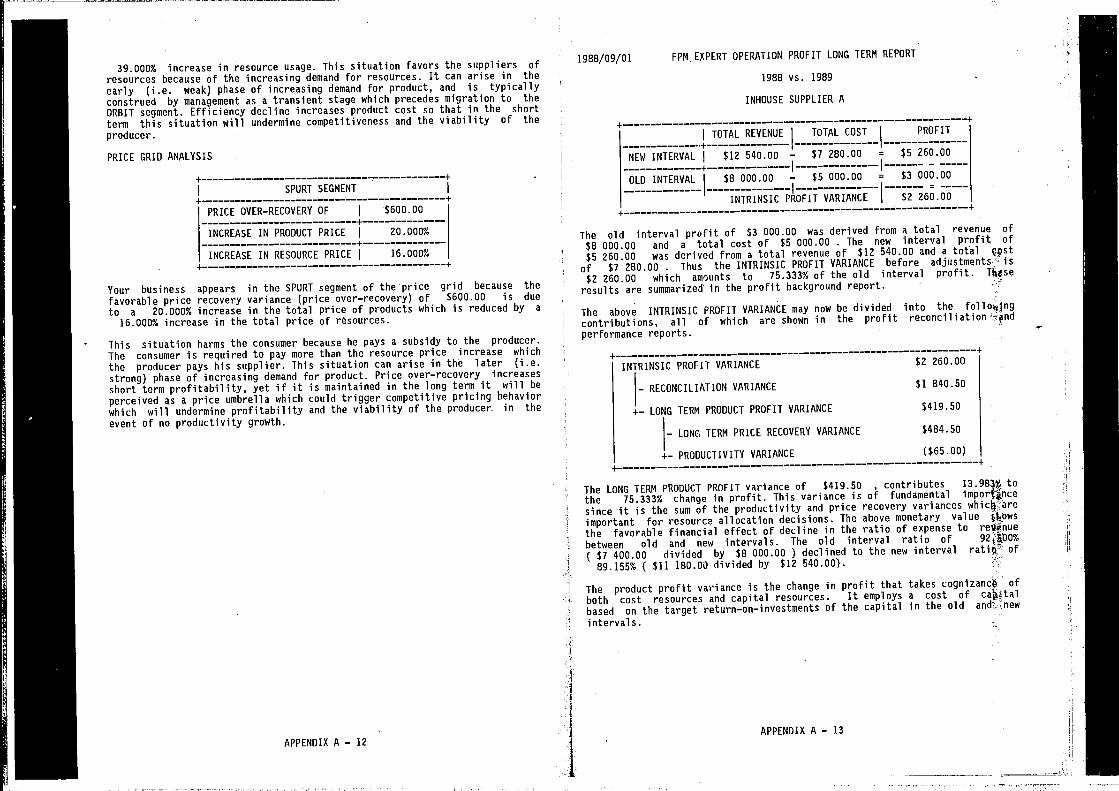
39.000% increase in resource usage. This situation favors the suppliers ofresources because of the increasing demand for resources. It can arise in the
early (i.e. weak) phase of increasing demand for product, and is typicallyconstrued by management as a transient stage which precedes migration to theORBIT segment. Efficiency decline increases product cost so that in the shortterm this situation will undermine competitiveness and the viability of the
producer.
PRICE GRID ANALYSIS
SPURT SEGMENT
+PRICE OVER—RECOVERY OF $600.00
+
INCREASE IN PRODUCT PRICE 20.000%+
INCREASE IN RESOURCE PRICE I16.000%
+
Your business appears in the SPURT segment of theprice grid because thefavorable price recovery variance (price over—recovery) of $600.00 is due
to a 20.000% increase in the total price of products which is reduced by a
16.000% increase in the total price of resources.
This situation harms the consumer because he pays a subsidy to the producer.The consumer is required to pay more than the resource price increase which
the producer pays his supplier. This situation can arise in the later (i.e.strong) phase of increasing demand for product. Price over—recovery increasesshort term profitability, yet if it is maintained in the long term it will beperceived as a price umbrella which could trigger competitive pricing behaviorwhich will undermine profitability and the viability of the producer- in the
event of no productivity growth.
APPENDIX A — 12
1988/09/01 FPM, EXPERT OPERATION PROFIT LONG TERM REPORT
1988 vs. 1989
INHOUSE SUPPLIER A
The old interval profit of $3 000.00 was derived from a total revenue of
$8 000.00 and a total cost of $5 000.00 . The new interval profit of
$5 260.00 was derived from a total revenue of $12 540.00 and a total çpst
of $7 280.00 . Thus the INTRINSIC PROFIT VARIANCE before adjustments Is
$2 260.00 which amounts to 75.333% of the old interval profit. These
results are summarized in the profit background report.
The above INTRINSIC PROFIT VARIANCE may now be divided into the followingcontributions, all of which are shown in the profitperformance reports.
The LONG TERM PRODUCT PROFIT variance of $419.50 contributes to
the 75.333% change in profit. This variance is of fundamental
since it is the sum of the productivity and price recovery variancesimportant for resource allocation decisions. The above monetary value shows
the favorable financial effect of decline in the ratio of expense to re$nue
between old and new intervals. The old interval ratio of 92J0O%
$7 400.00 divided by $8 000.00 ) declined to the new interval of89.155% ($11 180.00 divided by $12 540.00).
The product profit variance is the change in profit that takes cognizance of
both cost resources and capital resources. It employs a cost of c4italbased on the target return—on—investments of the capital in the oldintervals. -
APPENDIX A — 13
TOTAL REVENUE TOTAL COST PROFIT
—-F
NEW INTERVAL $12 540.00 — $7 280.00 = $5 260.00
+ I I
OLD INTERVAL $8 000.00 — $5 000.00 = $3 000.00
INTRINSIC PROFIT VARIANCE I$2 260.00
+INTRINSIC PROFIT VARIANCE $2 260.00
RECONCILIATION VARIANCE $1 840.50
+— LONG TERM PRODUCT PROFIT VARIANCE $419.50
LONG TERM PRICE RECOVERY VARIANCE $484.50
+— PRODUCTIVITY VARIANCE ($65.00)+
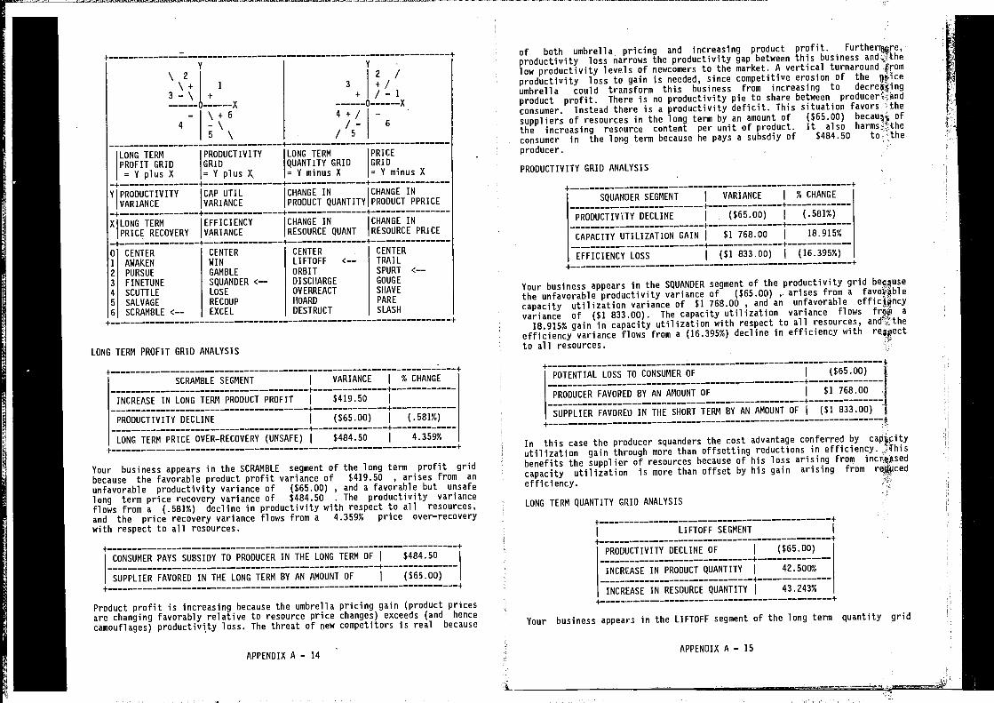
V\2\+ 1
3—\ ÷
— \+64 -\
5 \
Y
2 /3 +1
+ /—l—O —x
—
/— 6/5LONG TERMPROFIT GRID=YplusX
PRODUCTIVITYGRID=YplusX
LONG TERMQUANTITY GRID=YminusX
PRICEGRID=YminusX
PRODUCTIVITYVARIANCE
CAP UTILVARIANCE
CHANGE INPRODUCT QUANTITY
CHANGE INPRODUCT PPRICE
LONG TERNPRICE RECOVERY
EFFICIENCYVARIANCE
CHANGE INRESOURCE QUANT
CHANGE INRESOURCE PRICE
0 CENTER
1 AWAKEN
2 PURSUE
3 FINETUNE4 SCUTTLE5 SALVAGE6 SCRANBLE <——
CENTERWINGANBLESQUANDER c——
LOSE
RECOUP
EXCEL
CENTERLIFTOFF <——
ORBITDISCHARGEOVERREACTHOARD
DESTRUCT
CENTERTRAILSPURT c——
GOUGE
SHAVEPARE
SLASH
LONG TERN PROFIT GRID ANALYSIS
I$419.50 I
- + +
PRODUCTIVITY DECLINE I($65.00) (.581%)
- + +
LONG TERM PRICE OVER—RECOVERY (UNSAFE) I$484.50
I4.359%
- +
Your business appears in the SCRAMBLE segment of the long term profit gridbecause the favorable product profit variance of $419.50 , arises from an
unfavorable productivity variance of ($65.00) , and a favorable but unsafe
long term price recovery variance of $484.50 . The productivity varianceflows from a (.581%) decline in productivity with respect to all resources,and the price recovery variance flows from a 4.359% price over—recoverywith respect to all resources.
CONSUMER PAYS SUBSIDY TO PRODUCER IN THE LONG TERN OF I$484.50
+
SUPPLIER FAVORED IN THE LONG TERN BY AN ANOUNT OF ($65.00)+
Product profit is increasing because the umbrella pricing gain (product pricesare changing favorably relative to resource price changes) exceeds (and hencecamouflages) productivity loss. The threat of new competitors is real because
APPENDIX A — 14
of both umbrella, pricing and increasing product profit. Furtherrisre,productivity loss narrows the productivity gap between this business and.Jthelow productivity levels of newcomers to the market. A vertical turnaround fromproductivity loss to gain is needed, since competitive erosion of the
umbrella could transform this business from increasing toproduct profit. There is no productivity pie to share betweenconsumer. Instead there is a productivity deficit. This situation favors
the long term by an amount of ($65.00) ofthe increasing resource content per unit of product. It also harms?theconsumer in the long term because he pays a subsdiy of $484.50 to 'theproducer.
PRODUCTIVITY GRID ANALYSIS
SQUANDER SEGMENT VARIANCE % CHANGE
- + +
PRODUCTIVITY DECLINE ($65.00)I
(.581%)
+ +
CAPACITY UTILIZATION GAIN I$1 768.00
I18.915%
+ +
EFFICIENCY' LOSS I($1 833.00) I
(16.395%)
Your business appears in the SQUANDER segment of the productivity grid becausethe unfavorable productivity variance of ($65.00) , arises from acapacity utilization variance of $1 768.00 , and an unfavorable effictjncyvariance of ($1 83300). The capacity utilization variance flows a
18.915% gain in capacity utilization with respect to all resources,a (16.395%) decline in efficiency with
to all resources.
POTENTIAL LOSS TO+
PRODUCER FAVORED BY AN ANOUNT OF I$1 768.00
+
SHORT TERN BY AN AMOUNT OF ($1 833.00)SUPPLIER FAVORED+
In this case the producer squanders the cost advantage conferred byutilization gain through more than offsetting reductions in efficiency.benefits the supplier of resources because of his loss arising from incrnsedcapacity utilization is more than offset by his gain arising from
efficiency.
LONG TERN QUANTITY GRID ANALYSIS -
V LIFTOFF SEGMENT
PRODUCTIVITY DECLINE OF I($65.00)
+
INCREASE IN PRODUCT QUANTITY 42.500%+
INCREASE IN RESOURCE QUANTITY I43.243%
Your business appears in the LIFTOFF segment of the long term quantity grid
APPENDIX A — 15
I
-flu
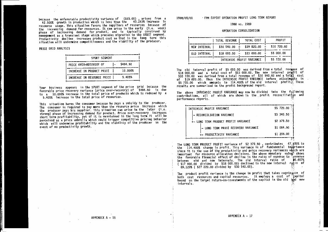
because the unfavorable productivity variance of ($65.00) , arises from a
42.500% growth in production which is less than the 43.243% ingrease inresource usage, This situation favors the suppliers of resources because .of
the increasing demand for resources. It can arise in the early (i.e. weak)
phase of increasing demand for product; and is typically construed bymanagement as a transient stage which precedes migration to the ORBIT segment.Productivity decline increases product cost so that in the long term thissituation will undermine competitiveness and the viability of the producer.
PRICE GRID ANALYSIS
SPURT SEGNENT
PRICE OVER—RECOVERY OF $484.50+
INCREASE IN PRODUCT PRICE j 10.000%+
INCREASE IN RESOURCE PRICE 5.405%
Your business appears in the SPURT segment of the price grid because thefavorable price recovery variance (price over—recovery) of $484.50 is due
to a 10.000% increase in the total price of products which is reduced by a
5.405% increase in the total price of resources.
This situation harms the consumer because he pays a subsidy to the producer.The consumer is required to pay more than the resource price increase which
the producer pays his supplier. This situation can arise in the later (i.e.strong) phase of increasing demand for product. Price over—recovery increasesshort term profitability, yet if it is maintained in the long term it will beperceived as a price umbrella which could trigger competitive pr.icing behaviorwhich will undermine profitability and the viability of the producer in the
event of no productivity growth.
The old interval profit of $5 000.00 was derived from a total revanue of$18 000.00 and a total cost of $13 000.00. The new interval prjfit of$10 720.00 was derived from a total revenue of $30 540.00 and a totk$ cost
of $19 820.00. Thus the INTRINSIC PROFIT VARIANCE before is$5 720.00 which amounts to 114.400% of the old interval These
results are summadzed in the profit background report.
The above INTRINSIC PROFIT VARIANCE may now be divided into thecontributions, all of which are shown in the profit reconciliat%an and
performance reports.
The LONG TERN PRODUCT PROFIT variance of $2 379.50 , contributes tothe 114.400% change in profit. This variance is of fundamentalsince it is the sum of the productivity and price recovery variances wkjch areimportant for resource allocation decisions. The above monetary value showsthe favorable financial effect of decline in the ratio of expense tobetween old and new intervals. The old interval ratio of 96.667%
( $17 400.00 divided by $18 000.00) declined to the new interval r*tio of89.129% ($27 220.00 divided by $30 540.00). -
The product profit variance is the change in profit that takes ofboth cost resources and capital resources. It employs a cost of lapitalbased on the target return—on—investments of the capital in the old new
intervals.
1988/09/01 FPN EXPERT OPERATION PROFIT LONG TERN REPORT
1988 vs. 1989
OPERATION CONSOLIDATION
-NEW INTERVAL
!$30 540.00 $19 820.00
- I
OLD INTEIIVAL $18 000.00 — $13 000.00 = $5 000.00
$10 720.00
IRIIIRI $5 720.00
RECONCILIATION VARIANCE $3 340.50 -
+— LONG TERM PRODUCT PROFIT VARIANCE $2 379.50
LONG TERN PRICE RECOVERY VARIANCE $1 084.50
+— PRODUCTIVITY VARIANCE $1 295.00
APPENDIX A — 16APPENDIX A — 17
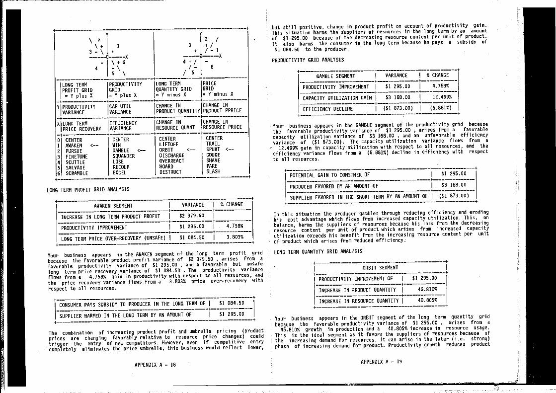
V\2\+ 1
3—\ +0 X
— \+64 —\
5 \
V
2 /3
+0 X
—
I— 6/5PRODUCTIVITY
GRID GRIDX = Y plus X
F— —
LONG TERMQUANTITY GRID= Y minus X
PRICEGRID= Yminus X
—
CAP UTIL CHANGE IN CHANGE IN
VARIANCE PRODUCT QUANTITY PRODUCT PPRICE- F- + -
EFFICIENCY CHANGE IN CHANGE IN
RECOVERY VARIANCE RESOURCE QUANT RESOURCE PRICE
CENTER
<—— WINGAMBLE C——
SQUANDER
LOSERECOUPEXCEL
CENTERLIFTOFFORBIT C——
DISCHARGEOVERREACTHOARD
DESTRUCT
CENTERTRAILSPURT <——
GOUGE
SHAVEPARESLASH
LONG TERM PROFIT GRID ANALYSIS
INCREASE IN LONG TERN PRODUCT PROFIT j $2 379.50
I$1 295.00 4.758%
+ +
LONG TERM PRICE OVER—RECOVERY (UNSAFE) I$1 084.50 I
3.803%
Your business appears in the AWAKEN segment of the long term profit gridbecause the favorable product profit variance of $2 379.50 , arises from a
favorable productivity variance of $1 295.00 , and a favorable but unsafe
long term price recovery variance of $1 084.50 . The productivity varianceflows from a 4.758% gain in productivity with respect to all resources, andthe price recovery variance flows from a 3.803% price over—recovery withrespect to all resources.
$1084.50
The combination of increasing product profit and umbrella pricing (productprices are changing favorably relative to resource price changes) could
trigger the entry of new competitors. However, even if competitive entry- completely eliminates the price umbrella, this business would reflect lower,
APPENDIX A —18
but still positive, change in product profit on account of productivity gain.This situation harms the of resources in the long term by an amount
of $1 295.00 because of the decreasing resource content per unit of product.It also harms the consumer in the long term because he pays a subsidy of$1 084.50 to the producer.
PRODUCTIVITY GRID ANALYSIS
GAMBLE SEGNENT
PRODUCTIVITY IMPROVEMENT
CAPACITY UTILIZATION GAIN
EFFICIENCY DECLINE
VARIANCE % CHANGE+
$1 295.00 I4.758%
+
$3 168.00 12.499%+
($1 873.00) I(6.881%)
Your business appears in the GAMBLE segment of the productivity grid because
the favorable productivity '!ariance of $1 295.00 , arises from a favorablecapacity utilization varlanre of $3 168.00 , and an unfavorable efficiencyvariance of ($1 873.00). The capacity utilization variance flows from a
12.499% gain in capacity utilization with respect to all resources, and theefficiency variance flows from a (6.881%) decline in efficiency with respectto all resources.
POTENTIAL GAIN TO CON&INER OF I
+
PRODUCER FAVORED BY AMOUNT OF ' $3 168.00
SUPPLIER FAVORED IN THE SHORT TERN BY AN AMOUNT OF ($1 873.00)+
+
In this situation the producer gambles through reducing efficiency and erodinghis cost advantage which flows from increased capacity utilization. This, on
balance, harms the suppliers of resources because his loss from the decreasingresource content per unit of product which arises from increased capacityutilization exceeds his benefit from the increasing resource content per unitof product which arises from reduced efficiency.
LONG TERM QUANTITY GRID ANALYSIS
PRODUCTIVITY IMPROVEMENT OFI
$1 295.00+
INCREASE IN PRODUCT QUANTITY I46.810%
+
INCREASE IN RESOURCE QUANTITY 40.805%+
Your business appears in the ORBIT segment of the long term quantity gridbecause the favorable productivity variance of $1 295.00 , arises from a
46.810% growth in production and a 40.805% increase in resource usage.
This is the ideal segment as it favors the suppliers of resources because ofthe increasing demand for resources. It can arise in the later (i.e. strong)phase of increasing demand for product. Productivity growth reduces product
APPENDIX A — 19
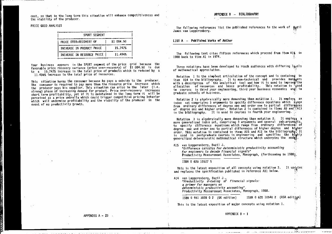
cost, so that in the long term this situation will enhance competitiveness andthe viability of the producer.
APPENDIX B — BIBLIOGRAPHY
The following references list the published references to the work ofJames van Loggerenberg.
The following text cites fifteen references which proceed from item in1988 back to item Al in 1974.
Your business appears in the SPURT segment of the price grid because thefavorable price recovery variance (price over—recovery) of $1 084.50 is due
to a 15.747% increase in the total price of products which is reduced by a
11.494% increase in the total price of resources.
This situation harms the consumer because he pays a subsidy to the producer.The consumer is required to pay more than the resource price increase whichthe producer pays his supplier. This situation can arise in the later (i.e.strong) phase of increasing demand for product. Price over—recovery increasesshort term profitability, yet if it is maintained in the long term it will beperceived as a price umbrella which could trigger competitive pricing behaviorwhich will undermine profitability and the viability of the producer in theevent of no productivity growth.
Three notations have been developed to reach audiences with differingof mathematical appreciation.
Notation 1 is the simplest articulation of the concept and is containe4 initem A14 in the bibliography. It is non—technical and provideswith a description of the analytical tool and how it is used toallocation of resources and hence profitability. This notation isin courses in third year engineering, third year business economics ingraduate schools of bjsiness.
Notation 2 is algebraically more demanding than notation 1. It employ; an
index set 3 arguments to specify difference equations whichfrom ordinary differences of degree one and order one to partial differodcesof degree one and higher order. Notation 2 is contained in items A9in the bibliography. It is used in courses in fourth year engineering.
Notation 3 is algebraically more demanding than notation 2. It a
more generalized index set, comprizing 3 arguments and severalto specify difference equations which range from ordinary differencer ofdegree one and order one to partial differences of higher degree and htgherorder. This notation is contained in items AlS and All in the Itis used in postgraduate courses in engineering and specifies thegeneralized deterministic mathematical structure which underpins the
A15 van Loggerenberg, Bazil J."Difference calculus for deterministic productivity accountingfor engineers to decode financial signals"Productivity Measurement Associates, Monograph, (forthcoming in
ISBN 0 620 10527 5
This is the latest exposition of all concepts using notation 3.and replaces the specification published in reference All below.
A14 van Loggerenberg, Bazil J.,"Productivity dncoding of financial signals:a primer for manngers ondeterministic productivity accounting".Productivity Measurement Associates, Monograph, 1988.
ISBN 0 951 3828 0 2 (UK edition)
It
ISBN 0 620 10540 2 (RSA
This is the latest exposition of major concepts using notation 1.
I
APPENDIX A — 20APPENDIX B —
PRICE GRID ANALYSIS
SPURT SEGMENT
PRICE OVER—RECOVERY OF $1 084.50+
INCREASE IN PRODUCT PRICE 15.747%+
INCREASE IN RESOURCE PRICEI
11.494%
LIST A — Published Works of Author
1988),
A13 van Loggerenberg, Basil J."A deterministic analysis of change in international unitlabor cost: import implications for U.S. industry"Managerial and Decision Economics
Vol. 8, 339—342 (1987)
This article is aimed at quantitative readers and presents a deterministicapproach to measure the relationship between productivity and unit labor costchange. The article employs the abridged notation cited under item E9 below.
A12 van Loggerenberg, Basil J."Deterministic productivity accounting for engineersto decode financial signals"S.A. Journal of Industrial Engineering
December 1987, Vol 1, No 2, (33 — 39)
This article provides engineers with an overview of the principal consepts.
All van Loggerenberg, Bazil J."Difference calculus for deterministic productivity accountingin the firm and in the economy"Productivity Measurement Inc., Monograph, 1986.
ISBN 0 620 09917 8 (1st edition)
This volume is aimed at mathematicians and presents the fully generalizednotation developed by the author to provide a comprehensive mathematicalspecification for deterministic productivity accounting. It updates itemA7 which is cited below. -
AlO van Loggerenberg, Basil J and Parsons, John"Tax rebates for productivity winners"The 5th World Productivity Congress,
Djarkata, Indonesia 1986, organised byThe World Confederation of Productivity Science.
This article aims at policy analysts and proposes a framework in whichfiscal policy can reward winners in the corporate productivity race. Thearticle is non—algebraic and addresses the issues raised by such a policyproposal.
A9 van toggerenberg, Basil J."The deterministic nexus between productivityand price change"South African Journal of Science
January 1986, vol 82 (34 — 45) ISSN 0038 2353
This article is aimed at mathematiciansd!terministic alternative to the customary
employed by econometrics to measure the relationship between productivity aqdprice change. The article presents an abridged version of thegeneralized notation specified in the PMI monograph cited in reference A)below.
A8 Visser, Jan H. and van Loggerenberg, Basil J."Product ivity and its proper measurement"South African Journal of Science
January 1986, vol 82 (21 — 23) ISSN 0038 2353
This article is aimed at scientists and brings to theirthe notion of productivity and its proper measurement in view Qtthe interest on the part of the authorities in linking the fundingteaching and research activities to productivity performance.
A7 van Loggerenberg, Basil J."A Mathematical Specification for Deterministic ProductivityAccounting in the Film and in the Economy",Productivity Measurement Inc., Monograph, November 1985,
ISBN 0 620 08958 X (1st edition)
This volume is aimed at mathematicians and presents the fully generalise4notation developed by the author to provide a comprehensive mathematica)specification for deterministic productivity accounting.
A6 van Loggerenberg, Basil J."Measuring business productivity",(Paper presented to theAmerican Institute for Decision Sciences
November 1983 Conference at San Antonio, Texas)
This article is aimed at business accountants and specifies geometricidentities to define variables. It reviews cost accounting measures andextends them with the additional measures introduced by the REALST model.
AS van Loggerenberg, Basil J."Deterministic growth accounting",DRI Statistician, December 1982
This article shows how a deterministic decomposition methodologycomprising a system of partial difference identities can be used tdvalidate stochastic models. The application entails testing part ofInput—Output model of DRI (Data Resources Inc.) which is the largest firmengaged in econometric modelling in the United States.
A4 van Loggerenberg, Basil J. and Cucchiaro, Stephen J."Productivity measurement and the bottom line",National Productivity , Winter 1981—82: 87—99.
This non—technical article is aimed at management and focusses on thephilosophy of the approach and on business applications.
APPENDIX B — 2
and presents a
stochastic approach
APPENDIX B — 3
A3 van Loggerenberg, Bazil J."Measuring telecommunications productivity"Telephony, 200(23): 28—31, 46, June 8, 1981.
This article contains a non—algebraic but technical, discussion of the workcovered by this approach.
A2 van Loggerenberg, Bazil J."Productivity targeting", inProductivity Measurement (An international review of
concepts, techniques, programmes and current issues)edited by David Bailey and Tony Hubert — 1980,ISBN 0—566—02230—3
This article is aimed at a technical audience but is non—algebraic incontent.
81 Sink, D.S."Organizational system performance: iscritical component?"Annual lIE Conrerence Proceedings, 1983
October 1974, Geneva)
This article is aimed at national accountants and statisticians. Itcontains an algebraic exposition of the imputation procedure employed bystatisticians to react to price change of a quality nature (including thoseinduced by technological change), and demonstrates flaws in suchprocedures.
LIST B — Citations In engineering literature
87 Parsons, John"Productivity Accounting and the Accountant"Pacific Rim International Productivity Conference,
American Institute of Industrial EngineersHawaii, February 1986.
B6 Sink, D.S.,"Productivity management: planning, measurement andevaluation, control and improvement",John Wiley & Son Inc., Monograph, 1985
ISBN 0—471—89176—2
LIST C — Citations in economics literature
C4 du Plooy, Roelf M.Productivity in South African Industry,South African Journal of Economics
Vol. 56 (1) , 82—93, (1988)
C3 Kendrick, John W."Improving Company Productivity"John Hopkins University Press, 1984
ISBN 0—8018—2992—5
C2 Guy, C.E., Brown, G.F., and O'Hara, D.J.,"A determinsitic profit attribution model— the postal service, a case study"
Managerial and Decision Economics 1983, 4(3) 208—213
CI Parsons, John"Profitability analysis in inter—firm comparison:A new approach", in
Productivity Measurement (An international review of
B5 Sink, D.S., Tuttle, T.C. and Devries, S.J.,"Productivity measurement and evaluation: what is available?"National Productivity Review, Summer 1984
concepts, techniques, programmes and current issues)edited by David Bailey and Tony Hubert — 1980,ISBN 0—566—02230—3
APPENDIX B — 4 APPENDIX B — 5
B4 Sink, D.S. and Devries, S.J.,"An in—depth study and review of the state—of—the—art andpractice productivity measurement techniques",Annual International lIE Conference Proceedings, 1984
B3 Swaim, J.C. and Sink, D.S.,"Productivity measurement in the service sector: ahotel/motel application of the multi—factor productivitymeasurementAnnual International lIE Conference Proceedings, 1984
Al van Loggerenberg, Bazil J.'Distortions in the existing price series"(Paper distributed to theUnited Nations Conference of Statisticians
B2 Swaim, J.C. ar,d Sink, D.S.,"Current in in firm orproductivity and evaluation",lIE Conference Proceedings, Fall, 1983
corporate level
a
LIST D — Citations in accounting literature
Dl Gordon, Paul N., and Parsons, John'Productivity: its impact on profits"Corporate Accounting Spring 1985, 3(2) 82—84
APPENDIX B — 6