SIGNALS AND SYSTEMS B.TECH

(II YEAR – I SEM) (2020-21)

DEPARTMENT OF ELECTRONICS AND COMMUNICATION ENGINEERING

MALLA REDDY COLLEGE OF ENGINEERING &TECHNOLOGY

(Autonomous Institution – UGC, Govt. of India) Recognized under 2(f) and 12 (B) of UGC ACT 1956

(Affiliated to JNTUH, Hyderabad, Approved by AICTE - Accredited by NBA & NAAC – ‘A’ Grade - ISO 9001:2015 Certified) Maisammaguda, Dhulapally (Post Via. Kompally), Secunderabad – 500100, Telangana State, India

MALLA REDDY COLLEGE OF ENGINEERING AND TECHNOLOGY II Year B.Tech ECE-I Sem L T/P/D C

3 -/-/- 3

(R18A0402) SIGNALS AND SYSTEMS OBJECTIVES:

The main objectives of the course are:

1. Coverage of continuous and discrete-time signals and representations and methods that is necessary for the analysis of continuous and discrete-time signals.

2. Knowledge of time-domain representation and analysis concepts as they relate to difference equations, impulse response and convolution, etc.

3. Knowledge of frequency-domain representation and analysis concepts using Fourier analysis tools, Z-transform.

4. Concepts of the sampling process. 5. Mathematical and computational skills needed in application areas like communication,

signal processing and control, which will be taught in other courses. UNIT I: INTRODUCTION TO SIGNALS: Elementary Signals- Continuous Time (CT) signals, Discrete Time (DT) signals, Classification of Signals ,Basic Operations on signals,. FOURIER SERIES: Representation of Fourier series, Continuous time periodic signals, Dirichlet’s conditions, Trigonometric Fourier Series, Exponential Fourier Series, Complex Fourier spectrum. UNIT II: FOURIER TRANSFORMS: Deriving Fourier transform from Fourier series, Fourier transform of arbitrary signal, Fourier transform of standard signals, Fourier transform of periodic signals, Properties of Fourier transforms. SAMPLING: Sampling theorem – Graphical and analytical proof for Band Limited Signals, impulse sampling, Natural and Flat top Sampling, Reconstruction of signal from its samples, effect of under sampling – Aliasing. UNIT III: SIGNAL TRANSMISSION THROUGH LINEAR SYSTEMS: Introduction to Systems, Classification of Systems, Linear Time Invariant (LTI) systems, impulse response, Transfer function of a LTI system. Filter characteristics of linear systems. Distortion less transmission through a system, Signal bandwidth, System bandwidth, Ideal LPF, HPF and BPF characteristics UNIT IV: CONVOLUTION AND CORRELATION OF SIGNALS: Concept of convolution in time domain, Cross correlation and auto correlation of functions, properties of correlation function, Energy density spectrum, Parseval’s theorem, Power density spectrum, Relation between convolution and correlation UNIT V: LAPLACE TRANSFORMS: Review of Laplace transforms, Inverse Laplace transform, Concept of region of convergence (ROC) for Laplace transforms, Properties of L.T’s relation between L.T’s, and F.T. of a signal. Z–TRANSFORMS: Concept of Z- Transform of a discrete sequence. Distinction between Laplace, Fourier and Z transforms, Region of convergence in Z-Transform, Inverse Z- Transform, Properties of Z-transforms.

TEXT BOOKS: 1. “Signals & Systems”, Special Edition – MRCET, McGraw Hill Publications, 2017 2. Signals, Systems & Communications - B.P. Lathi, BS Publications, 2003. 3. Signals and Systems - A.V. Oppenheim, A.S. Willsky and S.H. Nawab, PHI, 2nd Edn. 4. Signals and Systems – A. Anand Kumar, PHI Publications, 3rd edition.

REFERENCE BOOKS:

1. Signals & Systems - Simon Haykin and Van Veen,Wiley, 2nd Edition. 2. Network Analysis - M.E. Van Valkenburg, PHI Publications, 3rd Edn., 2000. 3. Fundamentals of Signals and Systems Michel J. Robert, MGH International Edition,

2008. 4. Signals, Systems and Transforms - C. L. Philips, J. M. Parr and Eve A. Riskin, Pearson

education.3rd Edition, 2004. OUTCOMES: After completion of the course, the student will be able to:

1. Represent any arbitrary signals in terms of complete sets of orthogonal functions and understands

2. Arbitrary signal (discrete) as Fourier transform to draw the spectrum. 3. Concepts of auto correlation and cross correlation and power Density Spectrum. 4. For a given system, response can be obtained using Laplace transform, properties and

ROC of L.T. 5. Study the continuous and discrete signal relation and relation between F.T., L.T. & Z.T,

properties, ROC of Z Transform

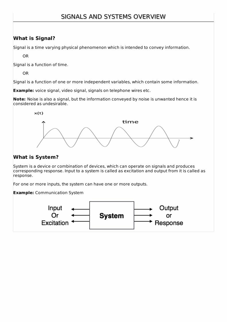
SIGNALS AND SYSTEMS OVERVIEWSIGNALS AND SYSTEMS OVERVIEW

What is Signal?Signal is a time varying physical phenomenon which is intended to convey information.

OR

Signal is a function of time.

OR

Signal is a function of one or more independent variables, which contain some information.

Example: voice signal, video signal, signals on telephone wires etc.

Note: Noise is also a signal, but the information conveyed by noise is unwanted hence it isconsidered as undesirable.

What is System?System is a device or combination of devices, which can operate on signals and producescorresponding response. Input to a system is called as excitation and output from it is called asresponse.

For one or more inputs, the system can have one or more outputs.

Example: Communication System

SIGNALS CLASSIFICATIONSIGNALS CLASSIFICATION

Signals are classified into the following categories:

Continuous Time and Discrete Time Signals

Deterministic and Non-deterministic Signals

Even and Odd Signals

Periodic and Aperiodic Signals

Energy and Power Signals

Real and Imaginary Signals

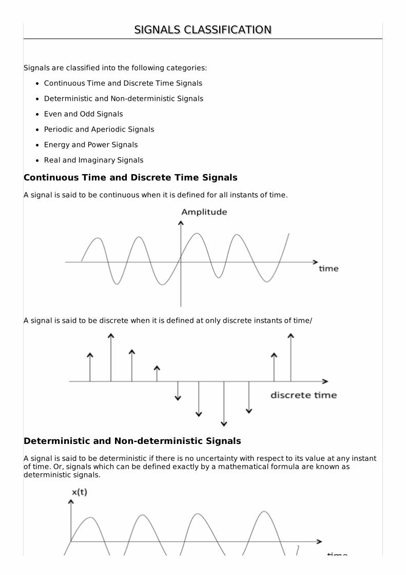
Continuous Time and Discrete Time SignalsA signal is said to be continuous when it is defined for all instants of time.

A signal is said to be discrete when it is defined at only discrete instants of time/

Deterministic and Non-deterministic SignalsA signal is said to be deterministic if there is no uncertainty with respect to its value at any instantof time. Or, signals which can be defined exactly by a mathematical formula are known asdeterministic signals.

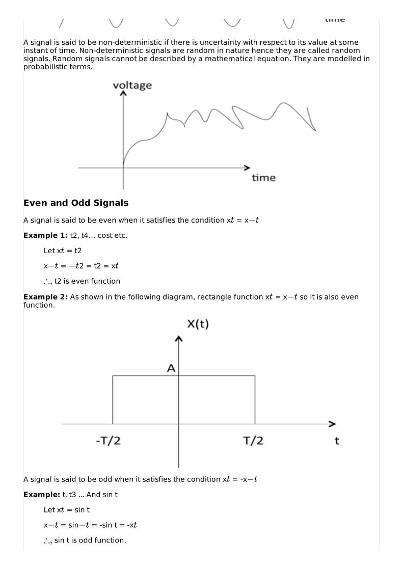
A signal is said to be non-deterministic if there is uncertainty with respect to its value at someinstant of time. Non-deterministic signals are random in nature hence they are called randomsignals. Random signals cannot be described by a mathematical equation. They are modelled inprobabilistic terms.

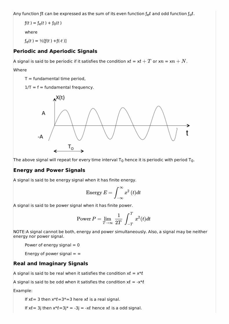
Even and Odd SignalsA signal is said to be even when it satisfies the condition x = x

Example 1: t2, t4… cost etc.

Let x = t2

x = 2 = t2 = x

t2 is even function

Example 2: As shown in the following diagram, rectangle function x = x so it is also evenfunction.

A signal is said to be odd when it satisfies the condition x = -x

Example: t, t3 ... And sin t

Let x = sin t

x = sin = -sin t = -x

sin t is odd function.

t −t

t

−t −t t

∴,

t −t

t −t

t

−t −t t

∴,

Any function ƒ can be expressed as the sum of its even function ƒe and odd function ƒo .

ƒ(t ) = ƒe(t ) + ƒ0(t )

where

ƒe(t ) = ½[ƒ(t ) +ƒ(-t )]

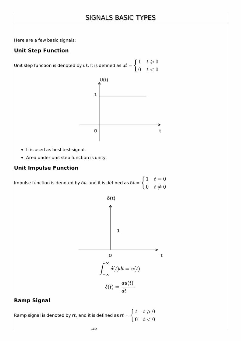
Periodic and Aperiodic Signals

A signal is said to be periodic if it satisfies the condition x = x or x = x .

Where

T = fundamental time period,

1/T = f = fundamental frequency.

The above signal will repeat for every time interval T0 hence it is periodic with period T0.

Energy and Power SignalsA signal is said to be energy signal when it has finite energy.

A signal is said to be power signal when it has finite power.

NOTE:A signal cannot be both, energy and power simultaneously. Also, a signal may be neitherenergy nor power signal.

Power of energy signal = 0

Energy of power signal = ∞

Real and Imaginary SignalsA signal is said to be real when it satisfies the condition x = x*

A signal is said to be odd when it satisfies the condition x = -x*

Example:

If x = 3 then x* =3*=3 here x is a real signal.

If x = 3j then x* =3j* = -3j = -x hence x is a odd signal.

t t t

t t + T n n + N

Energy E = (t)dt∫∞

−∞x2

Power P = (t)dtlimT→∞

12T

∫T

−T

x2

t t

t t

t t t

t t t t

Note: For a real signal, imaginary part should be zero. Similarly for an imaginary signal, real partshould be zero.

SIGNALS BASIC TYPESSIGNALS BASIC TYPES

Here are a few basic signals:

Unit Step Function

Unit step function is denoted by u . It is defined as u =

It is used as best test signal.Area under unit step function is unity.

Unit Impulse Function

Impulse function is denoted by δ . and it is defined as δ =

Ramp Signal

Ramp signal is denoted by r , and it is defined as r =

t t { 10

t ⩾ 0t < 0

t t { 10

t = 0t ≠ 0

δ(t)dt = u(t)∫∞

−∞

δ(t) =du(t)dt

t t { t

0t ⩾ 0t < 0

Area under unit ramp is unity.

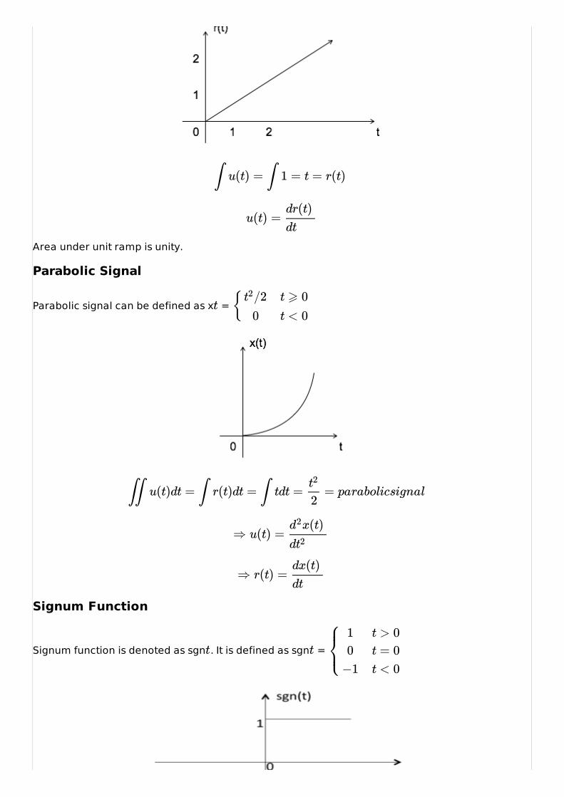
Parabolic Signal

Parabolic signal can be defined as x =

Signum Function

Signum function is denoted as sgn . It is defined as sgn =

∫ u(t) = ∫ 1 = t = r(t)

u(t) =dr(t)dt

t { /2t2

0

t ⩾ 0

t < 0

∬ u(t)dt = ∫ r(t)dt = ∫ tdt = = parabolicsignalt2

2

⇒ u(t) =x(t)d2

dt2

⇒ r(t) =dx(t)dt

t t

⎧⎩⎨⎪⎪

10

−1

t > 0t = 0t < 0

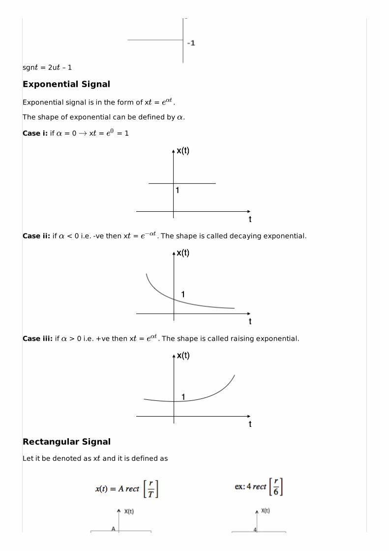
sgn = 2u – 1

Exponential Signal

Exponential signal is in the form of x = .

The shape of exponential can be defined by .

Case i: if = 0 x = = 1

Case ii: if < 0 i.e. -ve then x = . The shape is called decaying exponential.

Case iii: if > 0 i.e. +ve then x = . The shape is called raising exponential.

Rectangular SignalLet it be denoted as x and it is defined as

t t

t eαt

α

α → t e0

α t e−αt

α t eαt

t

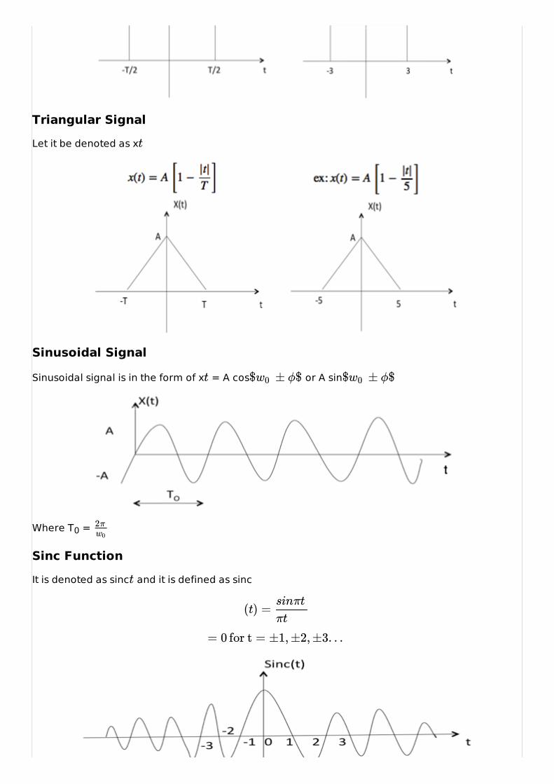
Triangular SignalLet it be denoted as x

Sinusoidal Signal

Sinusoidal signal is in the form of x = A cos or A sin

Where T0 =

Sinc FunctionIt is denoted as sinc and it is defined as sinc

t

t $ ± ϕ$w0 $ ± ϕ$w0

2πw0

t

(t) =sinπt

πt

= 0 for t = ±1, ±2, ±3. . .

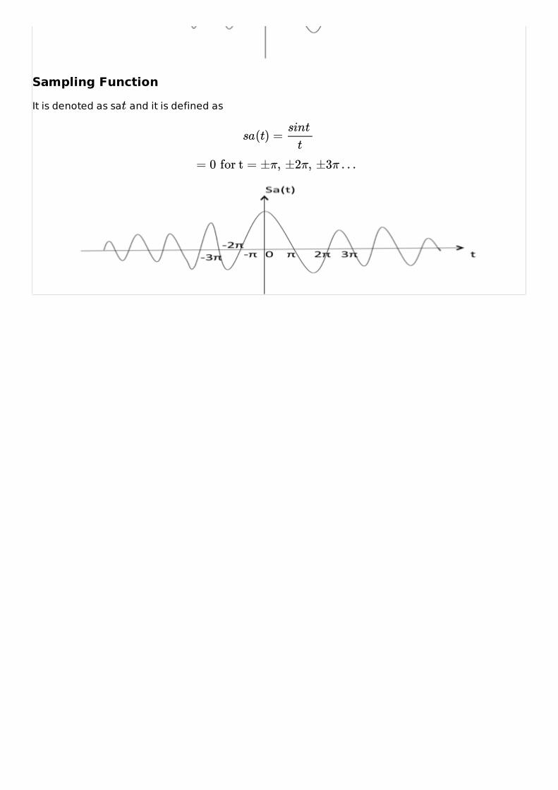
Sampling FunctionIt is denoted as sa and it is defined ast

sa(t) =sint

t

= 0 for t = ±π, ±2π, ±3π . . .

SIGNALS BASIC OPERATIONSSIGNALS BASIC OPERATIONS

There are two variable parameters in general:

1. Amplitude2. Time

The following operation can be performed with amplitude:

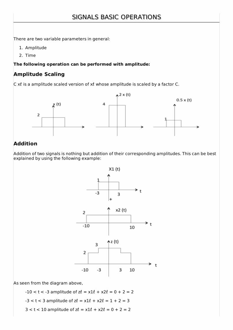
Amplitude ScalingC x is a amplitude scaled version of x whose amplitude is scaled by a factor C.

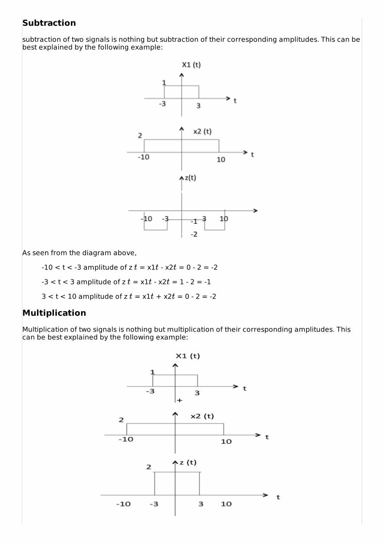
AdditionAddition of two signals is nothing but addition of their corresponding amplitudes. This can be bestexplained by using the following example:

As seen from the diagram above,

-10 < t < -3 amplitude of z = x1 + x2 = 0 + 2 = 2

-3 < t < 3 amplitude of z = x1 + x2 = 1 + 2 = 3

3 < t < 10 amplitude of z = x1 + x2 = 0 + 2 = 2

t t

t t t

t t t

t t t

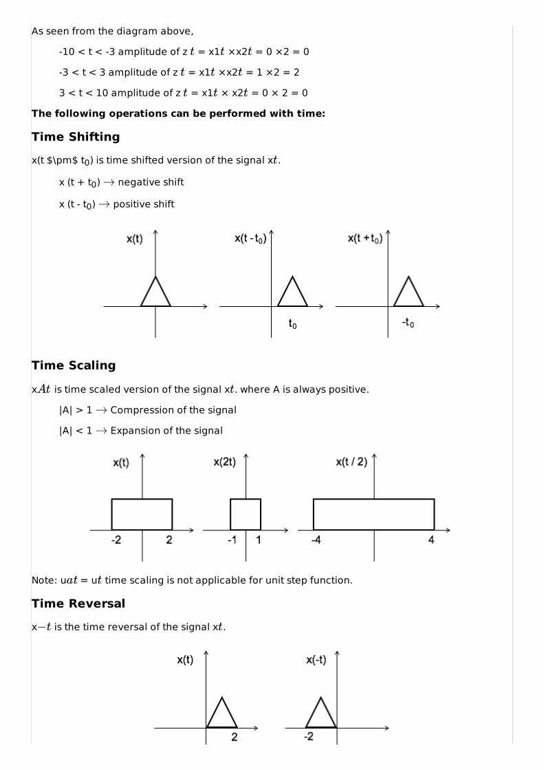
Subtractionsubtraction of two signals is nothing but subtraction of their corresponding amplitudes. This can bebest explained by the following example:

As seen from the diagram above,

-10 < t < -3 amplitude of z = x1 - x2 = 0 - 2 = -2

-3 < t < 3 amplitude of z = x1 - x2 = 1 - 2 = -1

3 < t < 10 amplitude of z = x1 + x2 = 0 - 2 = -2

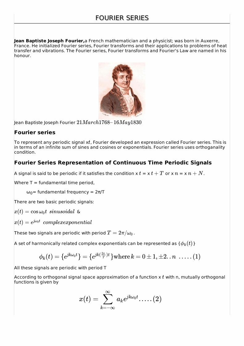
MultiplicationMultiplication of two signals is nothing but multiplication of their corresponding amplitudes. Thiscan be best explained by the following example:

t t t

t t t

t t t

As seen from the diagram above,

-10 < t < -3 amplitude of z = x1 ×x2 = 0 ×2 = 0

-3 < t < 3 amplitude of z = x1 ×x2 = 1 ×2 = 2

3 < t < 10 amplitude of z = x1 × x2 = 0 × 2 = 0

The following operations can be performed with time:

Time Shiftingx(t $\pm$ t0) is time shifted version of the signal x .

x (t + t0) negative shift

x (t - t0) positive shift

Time Scaling

x is time scaled version of the signal x . where A is always positive.

|A| > 1 Compression of the signal

|A| < 1 Expansion of the signal

Note: u = u time scaling is not applicable for unit step function.

Time Reversalx is the time reversal of the signal x .

t t t

t t t

t t t

t

→

→

At t

→

→

at t

−t t

FOURIER SERIESFOURIER SERIES

Jean Baptiste Joseph Fourier,a French mathematician and a physicist; was born in Auxerre,France. He initialized Fourier series, Fourier transforms and their applications to problems of heattransfer and vibrations. The Fourier series, Fourier transforms and Fourier's Law are named in hishonour.

Jean Baptiste Joseph Fourier

Fourier seriesTo represent any periodic signal x , Fourier developed an expression called Fourier series. This isin terms of an infinite sum of sines and cosines or exponentials. Fourier series uses orthoganalitycondition.

Fourier Series Representation of Continuous Time Periodic Signals

A signal is said to be periodic if it satisfies the condition x = x or x = x .

Where T = fundamental time period,

ω0= fundamental frequency = 2π/T

There are two basic periodic signals:

&

These two signals are periodic with period .

A set of harmonically related complex exponentials can be represented as { }

All these signals are periodic with period T

According to orthogonal signal space approximation of a function x with n, mutually orthogonalfunctions is given by

21March1768– 16May1830

t

t t+ T n n +N

x(t) = cos tω0 sinusoidal

x(t) = ej tω0 complexexponential

T = 2π/ω0

(t)ϕk

(t) = { } = { }wherek = 0± 1,±2. .n . . . . . (1)ϕk ejk tω0 ejk( )t2πT

t

x(t) = . . . . . (2)∑k=−∞

∞

akejk tω0

∞

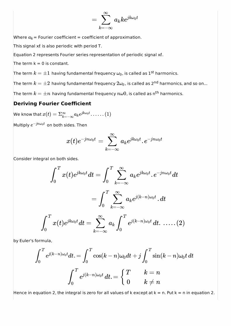
Where = Fourier coefficient = coefficient of approximation.

This signal x is also periodic with period T.

Equation 2 represents Fourier series representation of periodic signal x .

The term k = 0 is constant.

The term having fundamental frequency , is called as 1st harmonics.

The term having fundamental frequency , is called as 2nd harmonics, and so on...

The term having fundamental frequency , is called as nth harmonics.

Deriving Fourier Coefficient

We know that

Multiply on both sides. Then

Consider integral on both sides.

by Euler's formula,

Hence in equation 2, the integral is zero for all values of k except at k = n. Put k = n in equation 2.

= k∑k=−∞

∞

ak ejk tω0

ak

t

t

k = ±1 ω0

k = ±2 2ω0

k = ±n nω0

x(t) = . . . . . . (1)Σ∞k=−∞akejk tω0

e−jn tω0

x(t) = .e−jn tω0 ∑k=−∞

∞

akejk tω0 e−jn tω0

x(t) dt = . dt∫ T

0ejk tω0 ∫ T

0∑

k=−∞

∞

akejk tω0 e−jn tω0

= .dt∫ T

0∑

k=−∞

∞

akej(k−n) tω0

x(t) dt = dt. . . . . . (2)∫ T

0ejk tω0 ∑

k=−∞

∞

ak ∫ T

0ej(k−n) tω0

dt.= cos(k− n) dt+ j sin(k− n) t dt∫ T

0ej(k−n) tω0 ∫ T

0ω0 ∫ T

0ω0

dt.= {∫ T

0ej(k−n) tω0

T

0k = n

k ≠ n

T

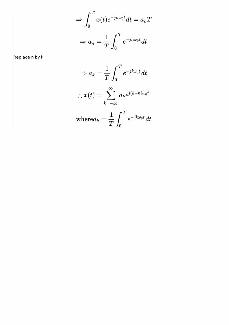
Replace n by k.

⇒ x(t) dt = T∫ T

0e−jn tω0 an

⇒ = dtan

1T

∫ T

0e−jn tω0

⇒ = dtak

1T

∫ T

0e−jk tω0

∴ x(t) = ∑k=−∞

∞

akej(k−n) tω0

where = dtak

1T

∫ T

0e−jk tω0

FOURIER SERIES PROPERTIESFOURIER SERIES PROPERTIES

These are properties of Fourier series:

Linearity Property

If &

then linearity property states that

Time Shifting Property

If

then time shifting property states that

Frequency Shifting Property

If

then frequency shifting property states that

Time Reversal Property

If

then time reversal property states that

If

Time Scaling Property

If

then time scaling property states that

If

Time scaling property changes frequency components from to .

Differentiation and Integration Properties

If

x(t) ← −−−−−−−−fourier series

− →−−−−−coefficient

fxn y(t) ← −−−−−−−−fourier series

− →−−−−−coefficient

fyn

a x(t) + b y(t) a + b← −−−−−−−−fourier series

− →−−−−−coefficient

fxn fyn

x(t) ← −−−−−−−−fourier series

− →−−−−−coefficient

fxn

x(t − )t0 ← −−−−−−−−fourier series

− →−−−−−coefficient

e−jnω0t0 fxn

x(t) ← −−−−−−−−fourier series

− →−−−−−coefficient

fxn

. x(t)ejnω0t0 ← −−−−−−−−fourier series

− →−−−−−coefficient

fx(n− )n0

x(t) ← −−−−−−−−fourier series

− →−−−−−coefficient

fxn

x(−t) ← −−−−−−−−fourier series

− →−−−−−coefficient

f−xn

x(t) ← −−−−−−−−fourier series

− →−−−−−coefficient

fxn

x(at) ← −−−−−−−−fourier series

− →−−−−−coefficient

fxn

ω0 aω0

x(t) ← −−−−−−−−fourier series

− →−−−−−coefficient

fxn

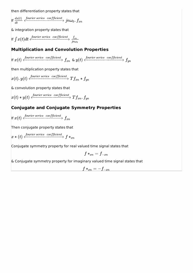
then differentiation property states that

If

& integration property states that

If

Multiplication and Convolution Properties

If &

then multiplication property states that

& convolution property states that

Conjugate and Conjugate Symmetry Properties

If

Then conjugate property states that

Conjugate symmetry property for real valued time signal states that

& Conjugate symmetry property for imaginary valued time signal states that

jn .dx(t)dt

← −−−−−−−−fourier series

− →−−−−−coefficient

ω0 fxn

∫ x(t)dt ← −−−−−−−−fourier series

− →−−−−−coefficient fxn

jnω0

x(t) ← −−−−−−−−fourier series

− →−−−−−coefficient

fxn y(t) ← −−−−−−−−fourier series

− →−−−−−coefficient

fyn

x(t). y(t) T ∗← −−−−−−−−fourier series

− →−−−−−coefficient

fxn fyn

x(t) ∗ y(t) T .← −−−−−−−−fourier series

− →−−−−−coefficient

fxn fyn

x(t) ← −−−−−−−−fourier series

− →−−−−−coefficient

fxn

x ∗ (t) f← −−−−−−−−fourier series

− →−−−−−coefficient

∗xn

f =∗xn f−xn

f = −∗xn f−xn

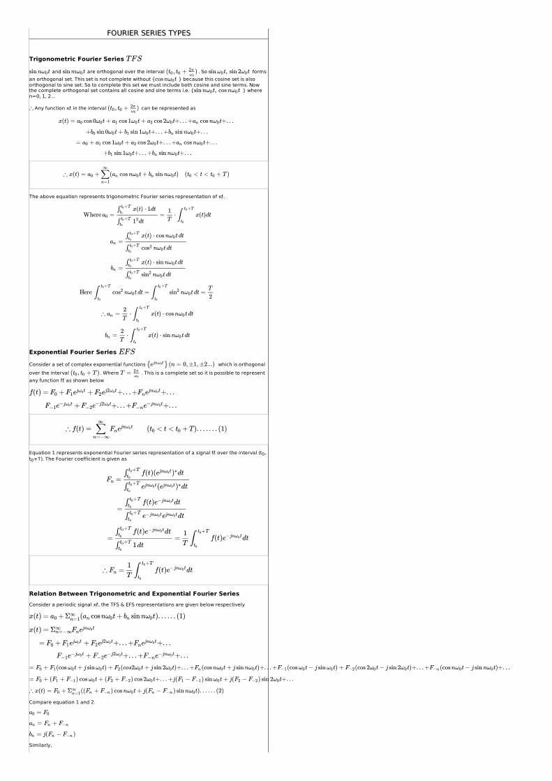
FOURIER SERIES TYPESFOURIER SERIES TYPES

Trigonometric Fourier Series

and are orthogonal over the interval . So formsan orthogonal set. This set is not complete without { } because this cosine set is alsoorthogonal to sine set. So to complete this set we must include both cosine and sine terms. Nowthe complete orthogonal set contains all cosine and sine terms i.e. { } wheren=0, 1, 2...

Any function x in the interval can be represented as

The above equation represents trigonometric Fourier series representation of x .

Exponential Fourier Series

Consider a set of complex exponential functions which is orthogonalover the interval . Where . This is a complete set so it is possible to representany function f as shown below

Equation 1 represents exponential Fourier series representation of a signal f over the interval (t0,t0+T). The Fourier coefficient is given as

Relation Between Trigonometric and Exponential Fourier SeriesConsider a periodic signal x , the TFS & EFS representations are given below respectively

Compare equation 1 and 2.

Similarly,

TFS

sin n tω0 sin m tω0 ( , + )t0 t02πω0

sin t, sin 2 tω0 ω0cos n tω0

sin n t, cos n tω0 ω0

∴ t ( , + )t0 t02πω0

x(t) = cos 0 t + cos 1 t + cos 2 t+. . . + cos n t+. . .a0 ω0 a1 ω0 a2 ω0 an ω0

+ sin 0 t + sin 1 t+. . . + sin n t+. . .b0 ω0 b1 ω0 bn ω0

= + cos 1 t + cos 2 t+. . . + cos n t+. . .a0 a1 ω0 a2 ω0 an ω0

+ sin 1 t+. . . + sin n t+. . .b1 ω0 bn ω0

∴ x(t) = + ( cos n t + sin n t) ( < t < + T )a0 ∑n=1

∞

an ω0 bn ω0 t0 t0

t

Where = = ⋅ x(t)dta0

x(t) ⋅ 1dt∫ +Tt0

t0

dt∫ +Tt0

t012

1T

∫+Tt0

t0

=an

x(t) ⋅ cos n t dt∫ +Tt0

t0ω0

n t dt∫ +Tt0

t0cos2 ω0

=bn

x(t) ⋅ sin n t dt∫ +Tt0

t0ω0

n t dt∫ +Tt0

t0sin2 ω0

Here n t dt = n t dt =∫+Tt0

t0

cos2 ω0 ∫+Tt0

t0

sin2 ω0T

2

∴ = ⋅ x(t) ⋅ cos n t dtan2T

∫+Tt0

t0

ω0

= ⋅ x(t) ⋅ sin n t dtbn2T

∫+Tt0

t0

ω0

EFS

{ } (n = 0, ±1, ±2...)ejn tω0

( , + T )t0 t0 T = 2πω0

t

f(t) = + + +. . . + +. . .F0 F1ej tω0 F2ej2 tω0 Fnejn tω0

+ +. . . + +. . .F−1e−j tω0 F−2e−j2 tω0 F−ne−jn tω0

∴ f(t) = ( < t < + T). . . . . . . (1)∑n=−∞

∞

Fnejn tω0 t0 t0

t

=Fn

f(t)( dt∫ +Tt0

t0ejn tω0 )∗

( dt∫ +Tt0

t0ejn tω0 ejn tω0 )∗

=f(t) dt∫ +Tt0

t0e−jn tω0

dt∫ +Tt0

t0e−jn tω0 ejn tω0

= = f(t) dtf(t) dt∫ +Tt0

t0e−jn tω0

1dt∫ +Tt0

t0

1T

∫ +Tt0

t0

e−jn tω0

∴ = f(t) dtFn

1T

∫ +Tt0

t0

e−jn tω0

t

x(t) = + ( cos n t + sin n t). . . . . . (1)a0 Σ∞n=1 an ω0 bn ω0

x(t) = Σ∞n=−∞Fnejn tω0

= + + +. . . + +. . .F0 F1ej tω0 F2ej2 tω0 Fnejn tω0

+ +. . . + +. . .F−1e−j tω0 F−2e−j2 tω0 F−ne−jn tω0

= + (cos t + j sin t) + (cos2 t + j sin 2 t)+. . . + (cos n t + j sin n t)+. . . + (cos t − j sin t) + (cos 2 t − j sin 2 t)+. . . + (cos n t − j sin n t)+. . .F0 F1 ω0 ω0 F2 ω0 ω0 Fn ω0 ω0 F−1 ω0 ω0 F−2 ω0 ω0 F−n ω0 ω0

= + ( + ) cos t + ( + ) cos 2 t+. . . +j( − ) sin t + j( − ) sin 2 t+. . .F0 F1 F−1 ω0 F2 F−2 ω0 F1 F−1 ω0 F2 F−2 ω0

∴ x(t) = + (( + ) cos n t + j( − ) sin n t). . . . . . (2)F0 Σ∞n=1 Fn F−n ω0 Fn F−n ω0

=a0 F0

= +an Fn F−n

= j( − )bn Fn F−n

= ( − j )1

= ( − j )Fn12

an bn

= ( + j )F−n12

an bn

FOURIER TRANSFORMSFOURIER TRANSFORMS

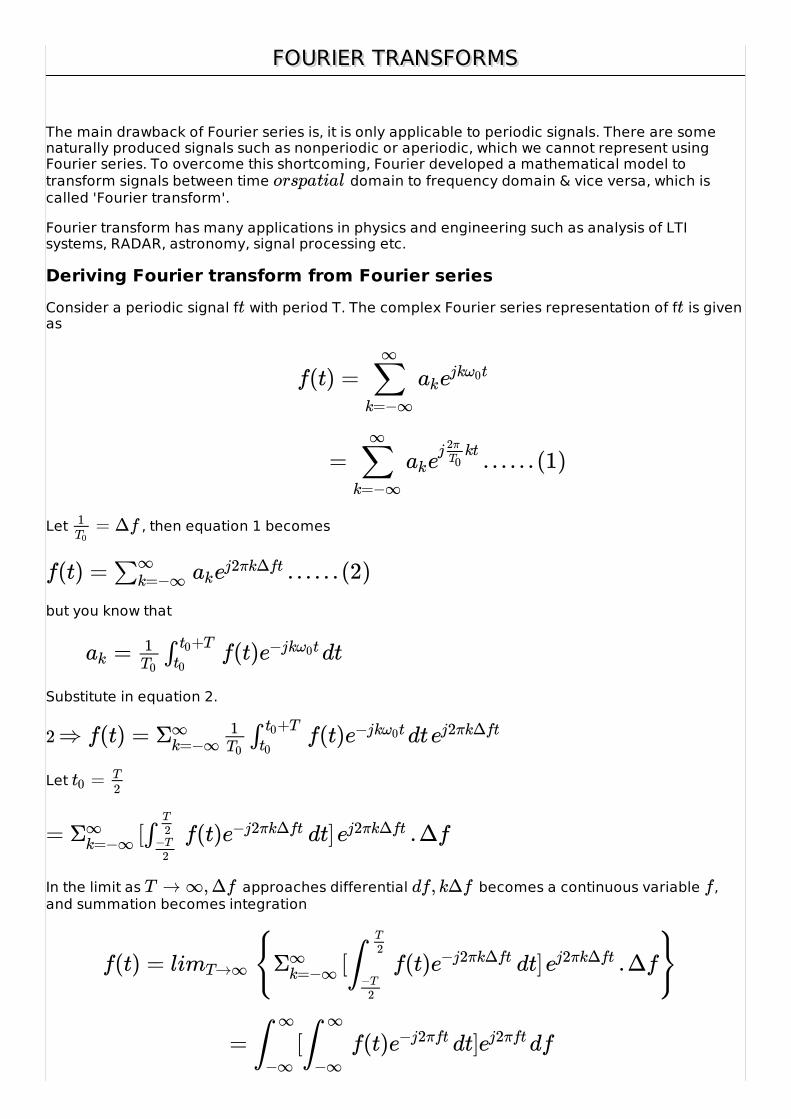
The main drawback of Fourier series is, it is only applicable to periodic signals. There are somenaturally produced signals such as nonperiodic or aperiodic, which we cannot represent usingFourier series. To overcome this shortcoming, Fourier developed a mathematical model totransform signals between time domain to frequency domain & vice versa, which iscalled 'Fourier transform'.

Fourier transform has many applications in physics and engineering such as analysis of LTIsystems, RADAR, astronomy, signal processing etc.

Deriving Fourier transform from Fourier seriesConsider a periodic signal f with period T. The complex Fourier series representation of f is givenas

Let , then equation 1 becomes

but you know that

Substitute in equation 2.

Let

In the limit as approaches differential becomes a continuous variable ,and summation becomes integration

orspatial

t t

f(t) = ∑k=−∞

∞

akejk tω0

= .. . . . . (1)∑k=−∞

∞

akej kt2π

T0

= Δf1T0

f(t) = . . . . . . (2)∑∞k=−∞ akej2πkΔft

= f(t) dtak1T0

∫ +Tt0t0

e−jk tω0

2⇒ f(t) = f(t) dtΣ∞k=−∞

1T0

∫ +Tt0t0

e−jk tω0 ej2πkΔft

=t0T2

= [ f(t) dt] .ΔfΣ∞k=−∞ ∫

T2

−T2

e−j2πkΔft ej2πkΔft

T → ∞,Δf df, kΔf f

f(t) = li { [ f(t) dt] .Δf}mT→∞ Σ∞k=−∞ ∫

T2

−T2

e−j2πkΔft ej2πkΔft

= [ f(t) dt] df∫ ∞

−∞∫ ∞

−∞e−j2πft ej2πft

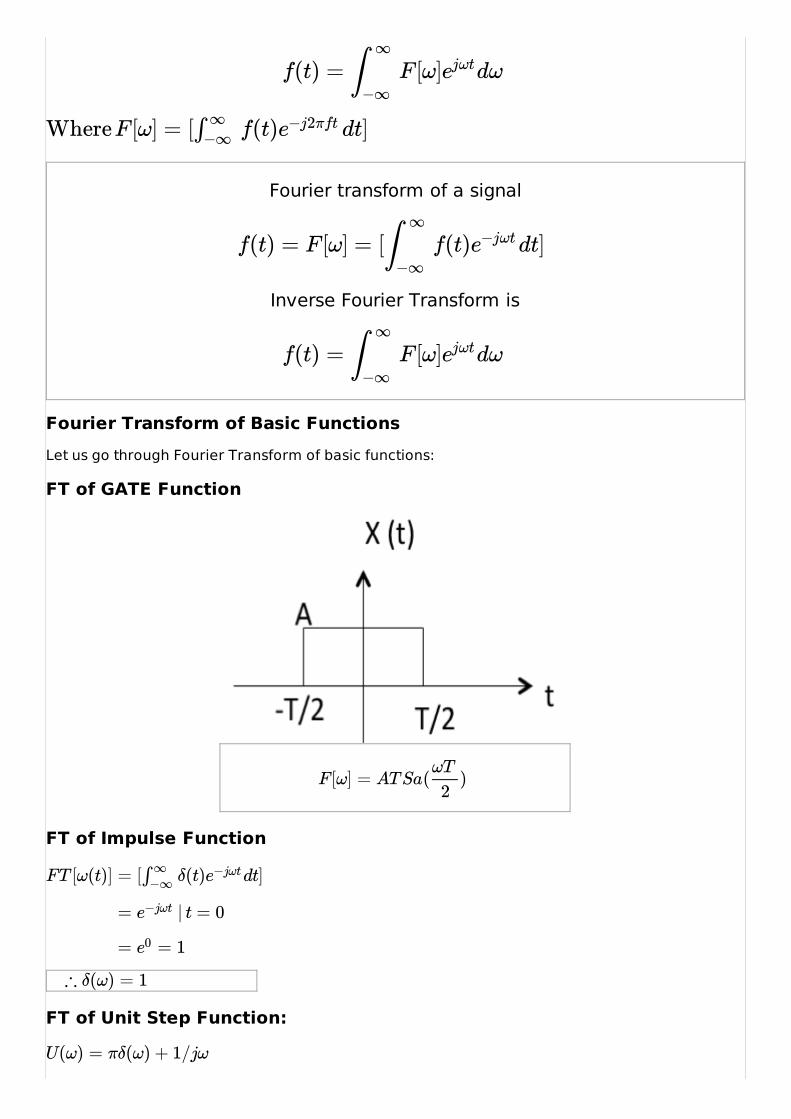
Fourier transform of a signal

Inverse Fourier Transform is

Fourier Transform of Basic FunctionsLet us go through Fourier Transform of basic functions:

FT of GATE Function

FT of Impulse Function

FT of Unit Step Function:

f(t) = F [ω] dω∫ ∞

−∞ejωt

WhereF [ω] = [ f(t) dt]∫ ∞−∞ e−j2πft

f(t) = F [ω] = [ f(t) dt]∫ ∞

−∞e−jωt

f(t) = F [ω] dω∫ ∞

−∞ejωt

F [ω] = AT Sa( )ωT

2

FT [ω(t)] = [ δ(t) dt]∫ ∞−∞ e−jωt

= | t = 0e−jωt

= = 1e0

∴ δ(ω) = 1

U(ω) = πδ(ω) + 1/jω

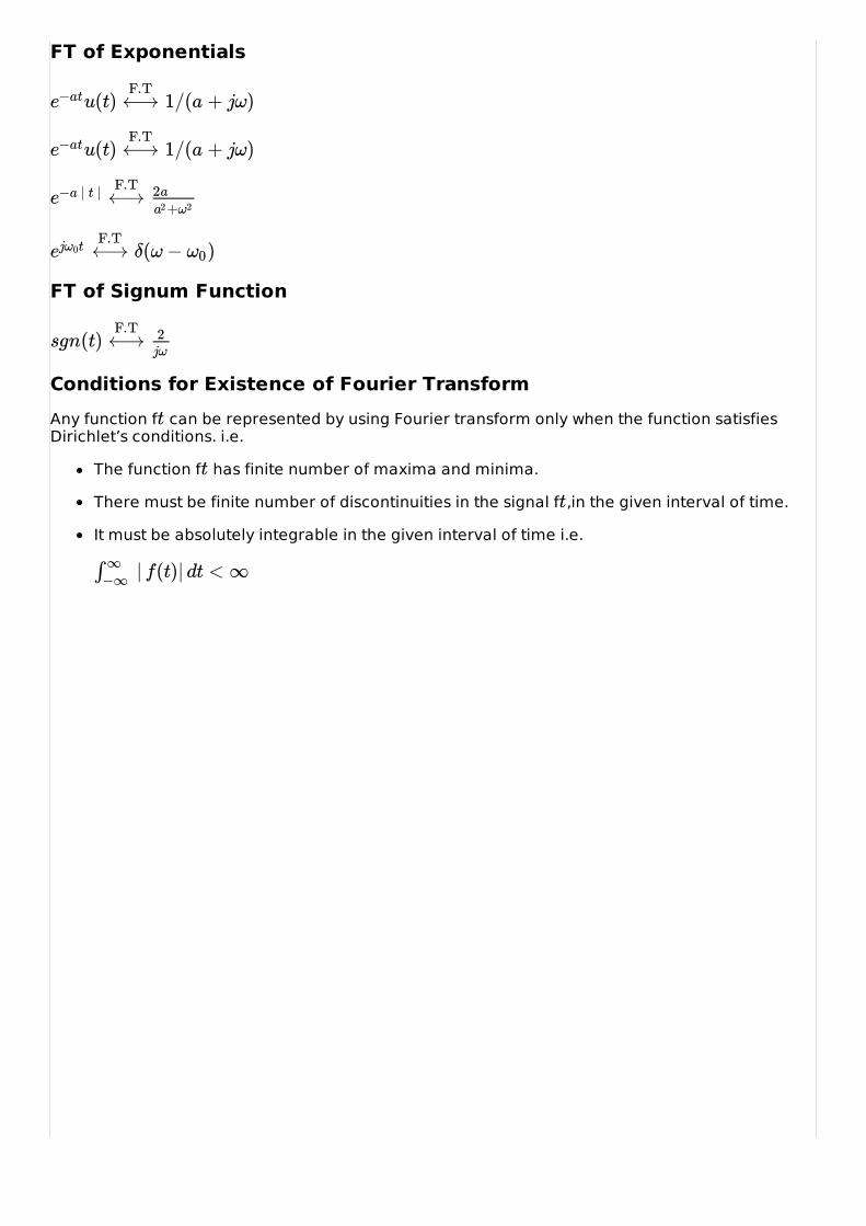
FT of Exponentials

FT of Signum Function

Conditions for Existence of Fourier TransformAny function f can be represented by using Fourier transform only when the function satisfiesDirichlet’s conditions. i.e.

The function f has finite number of maxima and minima.

There must be finite number of discontinuities in the signal f ,in the given interval of time.

It must be absolutely integrable in the given interval of time i.e.

u(t) 1/(a + jω)e−at ⟷F.T

u(t) 1/(a + jω)e−at ⟷F.T

e−a | t | ⟷F.T 2a

+a2 ω2

δ(ω − )ej tω0 ⟷F.T

ω0

sgn(t) ⟷F.T 2

jω

t

t

t

| f(t)| dt < ∞∫ ∞−∞

1 ∫π

FOURIER TRANSFORMS PROPERTIESFOURIER TRANSFORMS PROPERTIES

Here are the properties of Fourier Transform:

Linearity Property

Then linearity property states that

Time Shifting Property

Then Time shifting property states that

Frequency Shifting Property

Then frequency shifting property states that

Time Reversal Property

Then Time reversal property states that

Time Scaling Property

Then Time scaling property states that

Differentiation and Integration Properties

Then Differentiation property states that

If x(t) X(ω)⟷F.T

& y(t) Y (ω)⟷F.T

ax(t) + by(t) aX(ω) + bY (ω)⟷F.T

If x(t) X(ω)⟷F.T

x(t − ) X(ω)t0 ⟷F.T

e−jωt0

If x(t) X(ω)⟷F.T

. x(t) X(ω − )ej tω0 ⟷F.T

ω0

If x(t) X(ω)⟷F.T

x(−t) X(−ω)⟷F.T

If x(t) X(ω)⟷F.T

x(at) X1| a |

ωa

If x(t) X(ω)⟷F.T

and integration property states that

Multiplication and Convolution Properties

Then multiplication property states that

and convolution property states that

jω. X(ω)dx(t)dt

⟷F.T

(jω . X(ω)x(t)dn

dtn ⟷F.T

)n

∫ x(t) dt X(ω)⟷F.T 1

jω

∭ . . . ∫ x(t) dt X(ω)⟷F.T 1

(jω)n

If x(t) X(ω)⟷F.T

& y(t) Y (ω)⟷F.T

x(t). y(t) X(ω) ∗ Y (ω)⟷F.T

x(t) ∗ y(t) X(ω). Y (ω)⟷F.T 1

2π

SIGNALS SAMPLING THEOREMSIGNALS SAMPLING THEOREM

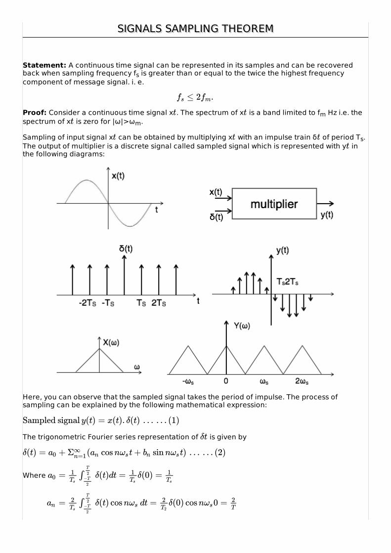
Statement: A continuous time signal can be represented in its samples and can be recoveredback when sampling frequency fs is greater than or equal to the twice the highest frequencycomponent of message signal. i. e.

Proof: Consider a continuous time signal x . The spectrum of x is a band limited to fm Hz i.e. thespectrum of x is zero for |ω|>ωm.

Sampling of input signal x can be obtained by multiplying x with an impulse train δ of period Ts.The output of multiplier is a discrete signal called sampled signal which is represented with y inthe following diagrams:

Here, you can observe that the sampled signal takes the period of impulse. The process ofsampling can be explained by the following mathematical expression:

The trigonometric Fourier series representation of is given by

Where

≤ 2 .fs fm

t tt

t t tt

Sampled signal y(t) = x(t). δ(t) . . . . . . (1)

δt

δ(t) = + ( cos n t + sin n t) . . . . . . (2)a0 Σ∞n=1 an ωs bn ωs

= δ(t)dt = δ(0) =a01Ts

∫T

2−T

2

1Ts

1Ts

= δ(t) cos n dt = δ(0) cos n 0 =an2Ts

∫T

2−T

2

ωs2T2

ωs2T

T

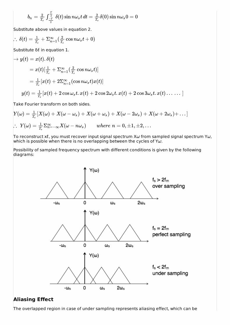
Substitute above values in equation 2.

Substitute δ in equation 1.

Take Fourier transform on both sides.

To reconstruct x , you must recover input signal spectrum X from sampled signal spectrum Y ,which is possible when there is no overlapping between the cycles of Y .

Possibility of sampled frequency spectrum with different conditions is given by the followingdiagrams:

Aliasing EffectThe overlapped region in case of under sampling represents aliasing effect, which can be

= δ(t) sin n t dt = δ(0) sin n 0 = 0bn2Ts

∫T

2−T

2

ωs2Ts

ωs

∴ δ(t) = + ( cos n t + 0)1Ts

Σ∞n=1

2Ts

ωs

t

→ y(t) = x(t). δ(t)

= x(t)[ + ( cos n t)]1Ts

Σ∞n=1

2Ts

ωs

= [x(t) + 2 (cos n t)x(t)]1Ts

Σ∞n=1 ωs

y(t) = [x(t) + 2 cos t. x(t) + 2 cos 2 t. x(t) + 2 cos 3 t. x(t) . . . . . . ]1Ts

ωs ωs ωs

Y (ω) = [X(ω) + X(ω − ) + X(ω + ) + X(ω − 2 ) + X(ω + 2 )+ . . . ]1Ts

ωs ωs ωs ωs

∴ Y (ω) = X(ω − n ) where n = 0, ±1, ±2, . . .1Ts

Σ∞n=−∞ ωs

t ω ωω

removed by

considering fs >2fm

By using anti aliasing filters.

SIGNALS SAMPLING TECHNIQUESSIGNALS SAMPLING TECHNIQUES

There are three types of sampling techniques:

Impulse sampling.

Natural sampling.

Flat Top sampling.

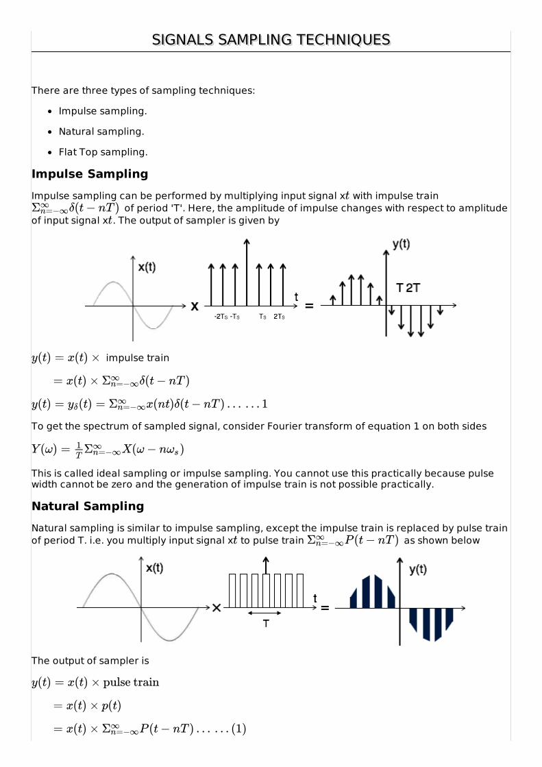
Impulse SamplingImpulse sampling can be performed by multiplying input signal x with impulse train

of period 'T'. Here, the amplitude of impulse changes with respect to amplitudeof input signal x . The output of sampler is given by

impulse train

To get the spectrum of sampled signal, consider Fourier transform of equation 1 on both sides

This is called ideal sampling or impulse sampling. You cannot use this practically because pulsewidth cannot be zero and the generation of impulse train is not possible practically.

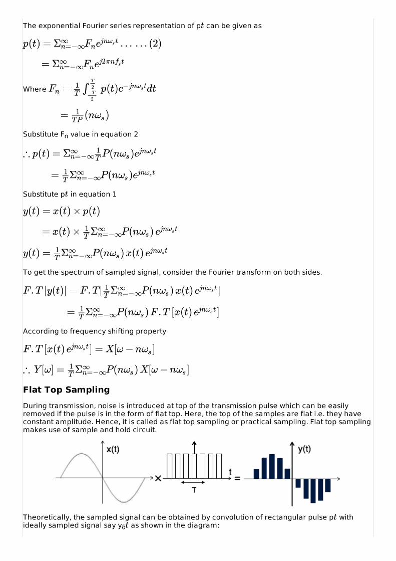
Natural SamplingNatural sampling is similar to impulse sampling, except the impulse train is replaced by pulse trainof period T. i.e. you multiply input signal x to pulse train as shown below

The output of sampler is

tδ(t − nT )Σ∞

n=−∞t

y(t) = x(t) ×

= x(t) × δ(t − nT )Σ∞n=−∞

y(t) = (t) = x(nt)δ(t − nT ) . . . . . . 1yδ Σ∞n=−∞

Y (ω) = X(ω − n )1T

Σ∞n=−∞ ωs

t P (t − nT )Σ∞n=−∞

y(t) = x(t) × pulse train

= x(t) × p(t)

= x(t) × P (t − nT ) . . . . . . (1)Σ∞n=−∞

The exponential Fourier series representation of p can be given as

Where

Substitute Fn value in equation 2

Substitute p in equation 1

To get the spectrum of sampled signal, consider the Fourier transform on both sides.

According to frequency shifting property

Flat Top SamplingDuring transmission, noise is introduced at top of the transmission pulse which can be easilyremoved if the pulse is in the form of flat top. Here, the top of the samples are flat i.e. they haveconstant amplitude. Hence, it is called as flat top sampling or practical sampling. Flat top samplingmakes use of sample and hold circuit.

Theoretically, the sampled signal can be obtained by convolution of rectangular pulse p withideally sampled signal say yδ as shown in the diagram:

t

p(t) = . . . . . . (2)Σ∞n=−∞Fnejn tωs

= Σ∞n=−∞Fnej2πn tfs

= p(t) dtFn1T

∫T

2−T

2

e−jn tωs

= (n )1TP

ωs

∴ p(t) = P(n )Σ∞n=−∞

1T

ωs ejn tωs

= P(n )1T

Σ∞n=−∞ ωs ejn tωs

t

y(t) = x(t) × p(t)

= x(t) × P(n )1T

Σ∞n=−∞ ωs ejn tωs

y(t) = P(n ) x(t)1T

Σ∞n=−∞ ωs ejn tωs

F . T [y(t)] = F . T [ P(n ) x(t) ]1T

Σ∞n=−∞ ωs ejn tωs

= P(n ) F . T [x(t) ]1T

Σ∞n=−∞ ωs ejn tωs

F . T [x(t) ] = X[ω − n ]ejn tωs ωs

∴ Y [ω] = P(n ) X[ω − n ]1T

Σ∞n=−∞ ωs ωs

tt

y(t) = p(t) × (t) . . . . . . (1)

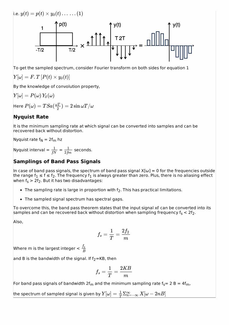
i.e.

To get the sampled spectrum, consider Fourier transform on both sides for equation 1

By the knowledge of convolution property,

Here

Nyquist RateIt is the minimum sampling rate at which signal can be converted into samples and can berecovered back without distortion.

Nyquist rate fN = 2fm hz

Nyquist interval = = seconds.

Samplings of Band Pass SignalsIn case of band pass signals, the spectrum of band pass signal X[ω] = 0 for the frequencies outsidethe range f1 ≤ f ≤ f2. The frequency f1 is always greater than zero. Plus, there is no aliasing effectwhen fs > 2f2. But it has two disadvantages:

The sampling rate is large in proportion with f2. This has practical limitations.

The sampled signal spectrum has spectral gaps.

To overcome this, the band pass theorem states that the input signal x can be converted into itssamples and can be recovered back without distortion when sampling frequency fs < 2f2.

Also,

Where m is the largest integer <

and B is the bandwidth of the signal. If f2=KB, then

For band pass signals of bandwidth 2fm and the minimum sampling rate fs= 2 B = 4fm,

the spectrum of sampled signal is given by

y(t) = p(t) × (t) . . . . . . (1)yδ

Y [ω] = F . T [P (t) × (t)]yδ

Y [ω] = P (ω) (ω)Yδ

P (ω) = T Sa( ) = 2 sin ωT /ωωT2

1fN

12fm

t

= =fs1T

2f2

m

f2

B

= =fs1T

2KB

m

Y [ω] = X[ω − 2nB]1T

Σ∞n=−∞

SYSTEMS CLASSIFICATIONSYSTEMS CLASSIFICATION

Systems are classified into the following categories:

Liner and Non-liner SystemsTime Variant and Time Invariant SystemsLiner Time variant and Liner Time invariant systemsStatic and Dynamic SystemsCausal and Non-causal SystemsInvertible and Non-Invertible SystemsStable and Unstable Systems

Liner and Non-liner SystemsA system is said to be linear when it satisfies superposition and homogenate principles. Considertwo systems with inputs as x1 , x2 , and outputs as y1 , y2 respectively. Then, according to thesuperposition and homogenate principles,

T [a1 x1 + a2 x2 ] = a1 T[x1 ] + a2 T[x2 ]

T [a1 x1 + a2 x2 ] = a1 y1 + a2 y2

From the above expression, is clear that response of overall system is equal to response ofindividual system.

Example:

= x2

Solution:

y1 = T[x1 ] = x12

y2 = T[x2 ] = x22

T [a1 x1 + a2 x2 ] = [ a1 x1 + a2 x2 ]2

Which is not equal to a1 y1 + a2 y2 . Hence the system is said to be non linear.

Time Variant and Time Invariant SystemsA system is said to be time variant if its input and output characteristics vary with time. Otherwise,the system is considered as time invariant.

The condition for time invariant system is:

y = y

The condition for time variant system is:

y y

Where y = T[x ] = input change

y = output change

Example:

t t t t

t t t t

∴, t t t t

t t

t t t

t t t

t t t t

t t

n, t n − t

n, t ≠ n − t

n, t n − t

n − t

y = x

y = T[x ] = x

y = x ) = x

y ≠ y . Hence, the system is time variant.

Liner Time variant and Liner Time Invariant Systems

If a system is both liner and time variant, then it is called liner time variant system.

If a system is both liner and time Invariant then that system is called liner time invariant system.

Static and Dynamic SystemsStatic system is memory-less whereas dynamic system is a memory system.

Example 1: y = 2 x

For present value t=0, the system output is y = 2x . Here, the output is only dependent uponpresent input. Hence the system is memory less or static.

Example 2: y = 2 x + 3 x

For present value t=0, the system output is y = 2x + 3x .

Here x is past value for the present input for which the system requires memory to get thisoutput. Hence, the system is a dynamic system.

Causal and Non-Causal SystemsA system is said to be causal if its output depends upon present and past inputs, and does notdepend upon future input.

For non causal system, the output depends upon future inputs also.

Example 1: y = 2 x + 3 x

For present value t=1, the system output is y = 2x + 3x .

Here, the system output only depends upon present and past inputs. Hence, the system is causal.

Example 2: y = 2 x + 3 x + 6x

For present value t=1, the system output is y = 2x + 3x + 6x Here, the system outputdepends upon future input. Hence the system is non-causal system.

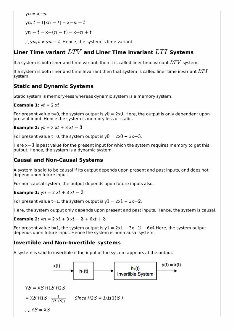
Invertible and Non-Invertible systemsA system is said to invertible if the input of the system appears at the output.

Y = X H1 H2

= X H1 · Since H2 = 1/ )

Y = X

n −n

n, t n − t −n − t

n − t −(n − t −n + t

∴ n, t n − t

LTV LTI

LT V

LT I

t t

0 0

t t t − 3

0 0 −3

−3

n t t − 3

1 1 −2

n t t − 3 t + 3

1 1 −2 4

S S S S

S S 1(H1(S))

S H1(S

∴, S S

t t

y = x

Hence, the system is invertible.

If y x , then the system is said to be non-invertible.

Stable and Unstable SystemsThe system is said to be stable only when the output is bounded for bounded input. For a boundedinput, if the output is unbounded in the system then it is said to be unstable.

Note: For a bounded signal, amplitude is finite.

Example 1: y = x2

Let the input is u then the output y = u2 = u = bounded output.

Hence, the system is stable.

Example 2: y =

Let the input is u then the output y = = ramp signal .

Hence, the system is unstable.

→ t t

t ≠ t

t t

t unitstepboundedinput t t t

t ∫ x(t) dt

t unitstepboundedinput t ∫ u(t) dtunboundedbecauseamplitudeoframpisnotfiniteitgoestoinfinitewhent$ → $infinite

CONVOLUTION AND CORRELATIONCONVOLUTION AND CORRELATION

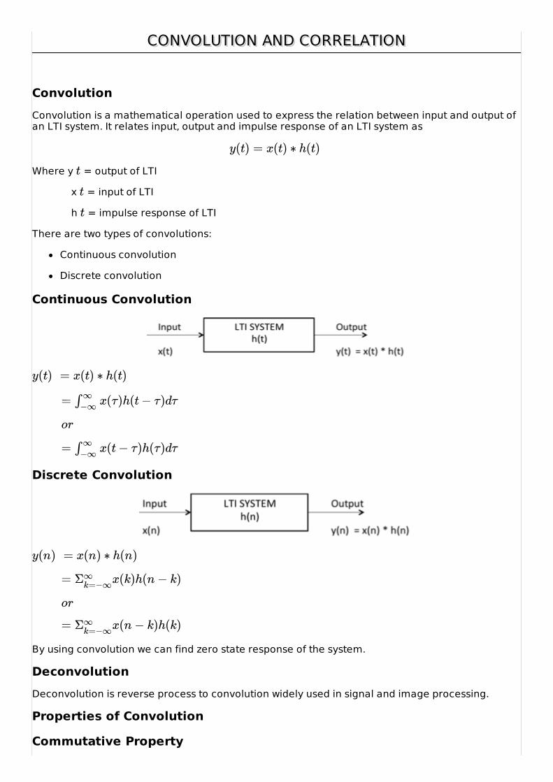
ConvolutionConvolution is a mathematical operation used to express the relation between input and output ofan LTI system. It relates input, output and impulse response of an LTI system as

Where y = output of LTI

x = input of LTI

h = impulse response of LTI

There are two types of convolutions:

Continuous convolution

Discrete convolution

Continuous Convolution

Discrete Convolution

By using convolution we can find zero state response of the system.

DeconvolutionDeconvolution is reverse process to convolution widely used in signal and image processing.

Properties of Convolution

Commutative Property

y(t) = x(t) ∗ h(t)

t

t

t

y(t) = x(t) ∗ h(t)

= x(τ)h(t − τ)dτ∫ ∞−∞

or

= x(t − τ)h(τ)dτ∫ ∞−∞

y(n) = x(n) ∗ h(n)

= x(k)h(n − k)Σ∞k=−∞

or

= x(n − k)h(k)Σ∞k=−∞

Distributive Property

Associative Property

Shifting Property

Convolution with Impulse

Convolution of Unit Steps

Scaling Property

If

then

Differentiation of Output

if

then

or

Note:

Convolution of two causal sequences is causal.

Convolution of two anti causal sequences is anti causal.

Convolution of two unequal length rectangles results a trapezium.

Convolution of two equal length rectangles results a triangle.

(t) ∗ (t) = (t) ∗ (t)x1 x2 x2 x1

(t) ∗ [ (t) + (t)] = [ (t) ∗ (t)] + [ (t) ∗ (t)]x1 x2 x3 x1 x2 x1 x3

(t) ∗ [ (t) ∗ (t)] = [ (t) ∗ (t)] ∗ (t)x1 x2 x3 x1 x2 x3

(t) ∗ (t) = y(t)x1 x2

(t) ∗ (t − ) = y(t − )x1 x2 t0 t0

(t − ) ∗ (t) = y(t − )x1 t0 x2 t0

(t − ) ∗ (t − ) = y(t − − )x1 t0 x2 t1 t0 t1

(t) ∗ δ(t) = x(t)x1

(t) ∗ δ(t − ) = x(t − )x1 t0 t0

u(t) ∗ u(t) = r(t)

u(t − ) ∗ u(t − ) = r(t − − )T1 T2 T1 T2

u(n) ∗ u(n) = [n + 1]u(n)

x(t) ∗ h(t) = y(t)

x(at) ∗ h(at) = y(at)1|a|

y(t) = x(t) ∗ h(t)

= ∗ h(t)dy(t)dt

dx(t)dt

= x(t) ∗dy(t)dt

dh(t)dt

A function convoluted itself is equal to integration of that function.

Example: You know that

According to above note,

Here, you get the result just by integrating .

Limits of Convoluted SignalIf two signals are convoluted then the resulting convoluted signal has following range:

Sum of lower limits < t < sum of upper limits

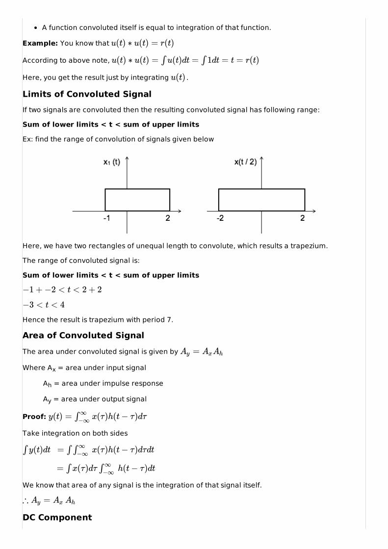
Ex: find the range of convolution of signals given below

Here, we have two rectangles of unequal length to convolute, which results a trapezium.

The range of convoluted signal is:

Sum of lower limits < t < sum of upper limits

Hence the result is trapezium with period 7.

Area of Convoluted SignalThe area under convoluted signal is given by

Where Ax = area under input signal

Ah = area under impulse response

Ay = area under output signal

Proof:

Take integration on both sides

We know that area of any signal is the integration of that signal itself.

DC Component

u(t) ∗ u(t) = r(t)

u(t) ∗ u(t) = ∫ u(t)dt = ∫ 1dt = t = r(t)

u(t)

−1 + −2 < t < 2 + 2

−3 < t < 4

=Ay AxAh

y(t) = x(τ)h(t − τ)dτ∫ ∞−∞

∫ y(t)dt = ∫ x(τ)h(t − τ)dτdt∫ ∞−∞

= ∫ x(τ)dτ h(t − τ)dt∫ ∞−∞

∴ =Ay Ax Ah

DC component of any signal is given by

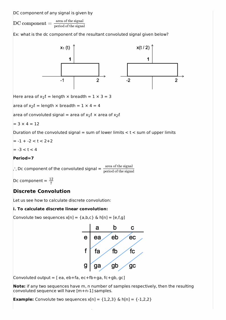
Ex: what is the dc component of the resultant convoluted signal given below?

Here area of x1 = length × breadth = 1 × 3 = 3

area of x2 = length × breadth = 1 × 4 = 4

area of convoluted signal = area of x1 × area of x2

= 3 × 4 = 12

Duration of the convoluted signal = sum of lower limits < t < sum of upper limits

= -1 + -2 < t < 2+2

= -3 < t < 4

Period=7

Dc component of the convoluted signal =

Dc component =

Discrete ConvolutionLet us see how to calculate discrete convolution:

i. To calculate discrete linear convolution:

Convolute two sequences x[n] = {a,b,c} & h[n] = [e,f,g]

Convoluted output = [ ea, eb+fa, ec+fb+ga, fc+gb, gc]

Note: if any two sequences have m, n number of samples respectively, then the resultingconvoluted sequence will have [m+n-1] samples.

Example: Convolute two sequences x[n] = {1,2,3} & h[n] = {-1,2,2}

DC component = area of the signalperiod of the signal

t

t

t t

∴ area of the signalperiod of the signal

127

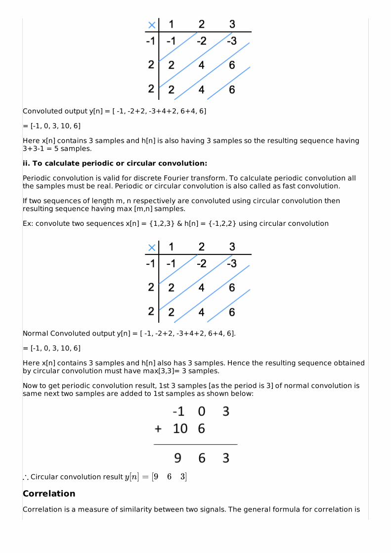
Convoluted output y[n] = [ -1, -2+2, -3+4+2, 6+4, 6]

= [-1, 0, 3, 10, 6]

Here x[n] contains 3 samples and h[n] is also having 3 samples so the resulting sequence having3+3-1 = 5 samples.

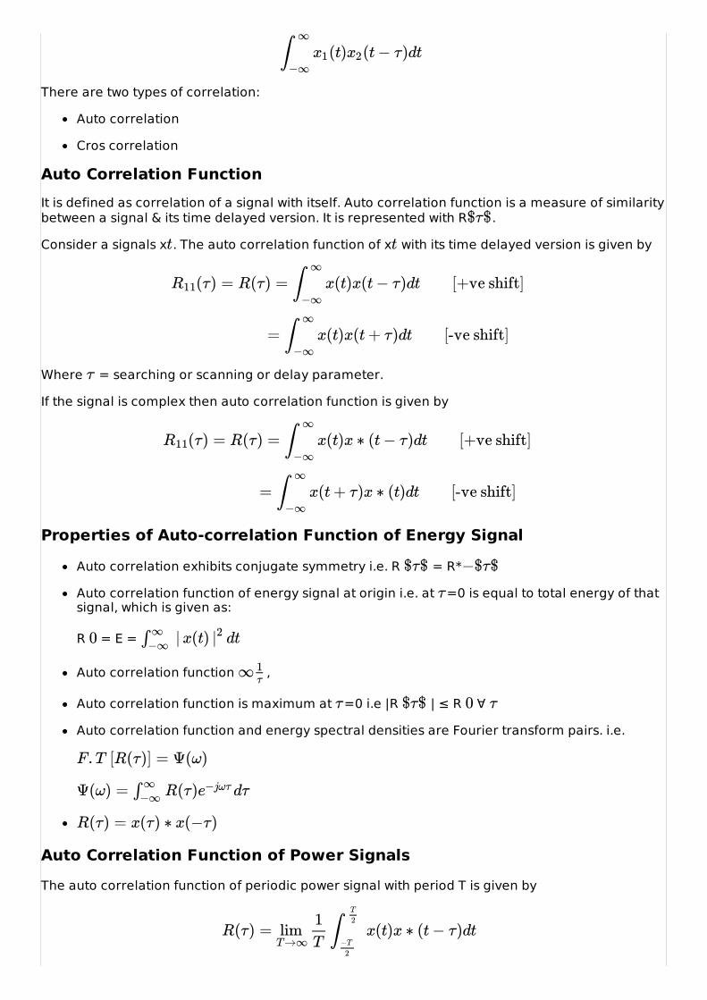
ii. To calculate periodic or circular convolution:

Periodic convolution is valid for discrete Fourier transform. To calculate periodic convolution allthe samples must be real. Periodic or circular convolution is also called as fast convolution.

If two sequences of length m, n respectively are convoluted using circular convolution thenresulting sequence having max [m,n] samples.

Ex: convolute two sequences x[n] = {1,2,3} & h[n] = {-1,2,2} using circular convolution

Normal Convoluted output y[n] = [ -1, -2+2, -3+4+2, 6+4, 6].

= [-1, 0, 3, 10, 6]

Here x[n] contains 3 samples and h[n] also has 3 samples. Hence the resulting sequence obtainedby circular convolution must have max[3,3]= 3 samples.

Now to get periodic convolution result, 1st 3 samples [as the period is 3] of normal convolution issame next two samples are added to 1st samples as shown below:

Circular convolution result

CorrelationCorrelation is a measure of similarity between two signals. The general formula for correlation is

∴ y[n] = [9 6 3]

∫∞

There are two types of correlation:

Auto correlation

Cros correlation

Auto Correlation FunctionIt is defined as correlation of a signal with itself. Auto correlation function is a measure of similaritybetween a signal & its time delayed version. It is represented with R .

Consider a signals x . The auto correlation function of x with its time delayed version is given by

Where = searching or scanning or delay parameter.

If the signal is complex then auto correlation function is given by

Properties of Auto-correlation Function of Energy Signal

Auto correlation exhibits conjugate symmetry i.e. R = R*

Auto correlation function of energy signal at origin i.e. at =0 is equal to total energy of thatsignal, which is given as:

R = E =

Auto correlation function ,

Auto correlation function is maximum at =0 i.e |R | ≤ R ∀

Auto correlation function and energy spectral densities are Fourier transform pairs. i.e.

Auto Correlation Function of Power SignalsThe auto correlation function of periodic power signal with period T is given by

(t) (t − τ)dt∫∞

−∞x1 x2

$τ$

t t

(τ) = R(τ) = x(t)x(t − τ)dt [+ve shift]R11 ∫∞

−∞

= x(t)x(t + τ)dt [-ve shift]∫∞

−∞

τ

(τ) = R(τ) = x(t)x ∗ (t − τ)dt [+ve shift]R11 ∫∞

−∞

= x(t + τ)x ∗ (t)dt [-ve shift]∫∞

−∞

$τ$ −$τ$

τ

0 | x(t) dt∫ ∞−∞ |2

∞ 1τ

τ $τ$ 0 τ

F . T [R(τ)] = Ψ(ω)

Ψ(ω) = R(τ) dτ∫ ∞−∞ e−jωτ

R(τ) = x(τ) ∗ x(−τ)

R(τ) = x(t)x ∗ (t − τ)dtlimT→∞

1T

∫T

2

−T

2

Properties

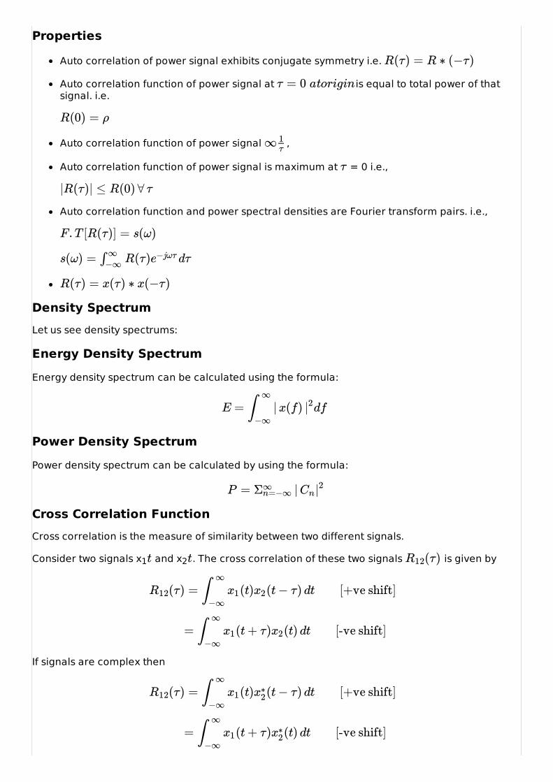
Auto correlation of power signal exhibits conjugate symmetry i.e.

Auto correlation function of power signal at is equal to total power of thatsignal. i.e.

Auto correlation function of power signal ,

Auto correlation function of power signal is maximum at = 0 i.e.,

Auto correlation function and power spectral densities are Fourier transform pairs. i.e.,

Density SpectrumLet us see density spectrums:

Energy Density SpectrumEnergy density spectrum can be calculated using the formula:

Power Density SpectrumPower density spectrum can be calculated by using the formula:

Cross Correlation FunctionCross correlation is the measure of similarity between two different signals.

Consider two signals x1 and x2 . The cross correlation of these two signals is given by

If signals are complex then

R(τ) = R ∗ (−τ)

τ = 0 atorigin

R(0) = ρ

∞ 1τ

τ

|R(τ)| ≤ R(0) ∀ τ

F . T [R(τ)] = s(ω)

s(ω) = R(τ) dτ∫ ∞−∞ e−jωτ

R(τ) = x(τ) ∗ x(−τ)

E = | x(f) df∫∞

−∞|2

P = |Σ∞n=−∞ Cn|2

t t (τ)R12

(τ) = (t) (t − τ) dt [+ve shift]R12 ∫∞

−∞x1 x2

= (t + τ) (t) dt [-ve shift]∫∞

−∞x1 x2

(τ) = (t) (t − τ) dt [+ve shift]R12 ∫∞

−∞x1 x∗

2

= (t + τ) (t) dt [-ve shift]∫∞

−∞x1 x∗

2

Properties of Cross Correlation Function of Energy and Power Signals

Auto correlation exhibits conjugate symmetry i.e. .

Cross correlation is not commutative like convolution i.e.

If R12 = 0 means, if , then the two signals are said to be orthogonal.

For power signal if then two signals are said to be orthogonal.

Cross correlation function corresponds to the multiplication of spectrums of one signal to thecomplex conjugate of spectrum of another signal. i.e.

This also called as correlation theorem.

Parsvel's TheoremParsvel's theorem for energy signals states that the total energy in a signal can be obtained by thespectrum of the signal as

Note: If a signal has energy E then time scaled version of that signal x has energy E/a.

(τ) = (t) (t − τ) dt [+ve shift]R21 ∫∞

−∞x2 x∗

1

= (t + τ) (t) dt [-ve shift]∫∞

−∞x2 x∗

1

(τ) = (−τ)R12 R∗21

(τ) ≠ (−τ)R12 R21

0 (t) (t)dt = 0∫ ∞−∞ x1 x∗

2

x(t) (t) dtlimT→∞1T

∫T

2−T

2

x∗

(τ) ←→ (ω) (ω)R12 X1 X∗2

E = |X(ω) dω12π

∫ ∞−∞ |2

at

DISTORTION LESS TRANSMISSIONDISTORTION LESS TRANSMISSION

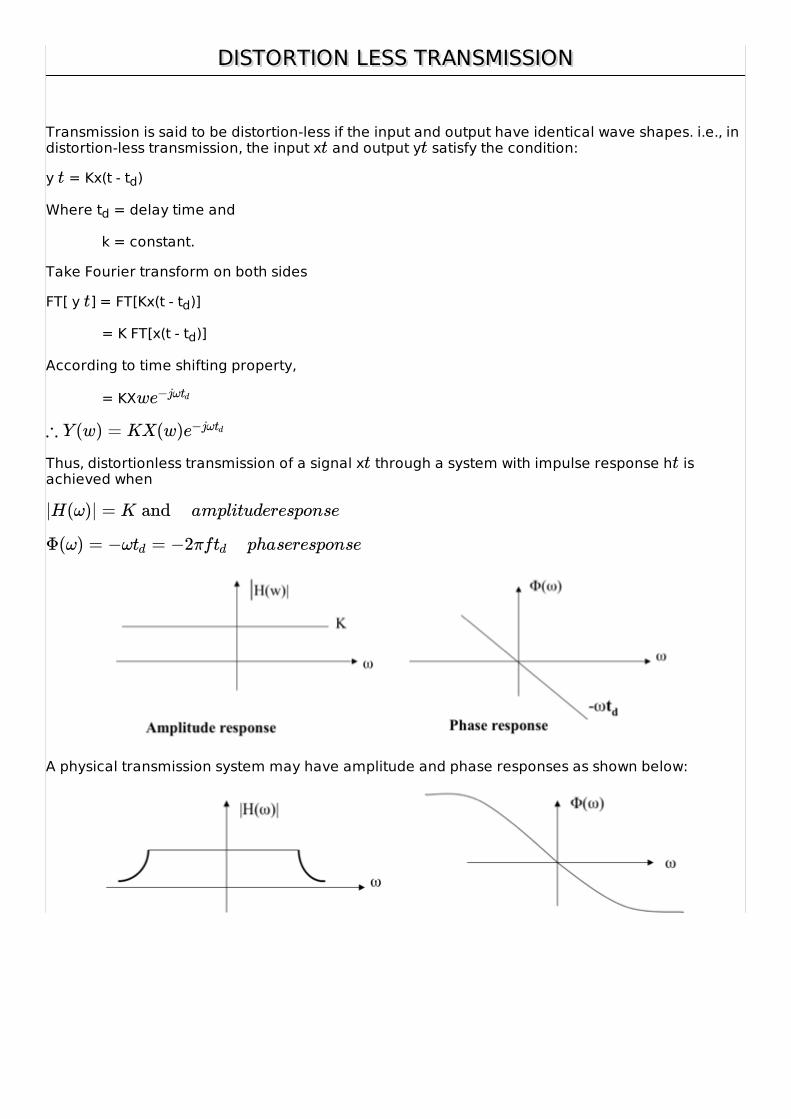
Transmission is said to be distortion-less if the input and output have identical wave shapes. i.e., indistortion-less transmission, the input x and output y satisfy the condition:

y = Kx(t - td)

Where td = delay time and

k = constant.

Take Fourier transform on both sides

FT[ y ] = FT[Kx(t - td)]

= K FT[x(t - td)]

According to time shifting property,

= KX

Thus, distortionless transmission of a signal x through a system with impulse response h isachieved when

A physical transmission system may have amplitude and phase responses as shown below:

t t

t

t

we−jωtd

∴ Y (w) = KX(w)e−jωtd

t t

|H(ω)| = K and amplituderesponse

Φ(ω) = −ω = −2πftd td phaseresponse

LAPLACE TRANSFORMS LAPLACE TRANSFORMS

Complex Fourier transform is also called as Bilateral Laplace Transform. This is used to solvedifferential equations. Consider an LTI system exited by a complex exponential signal of the form x = Gest.

Where s = any complex number = ,

σ = real of s, and

ω = imaginary of s

The response of LTI can be obtained by the convolution of input with its impulse response i.e.

Where H = Laplace transform of

Similarly, Laplace transform of

Relation between Laplace and Fourier transforms

Laplace transform of

Substitute s= σ + jω in above equation.

Inverse Laplace Transform

You know that

Here,

LLTT

t

σ + jω

y(t) = x(t) × h(t) = h(τ) x(t − τ)dτ∫ ∞−∞

= h(τ) G dτ∫ ∞−∞ es(t−τ)

= G . h(τ) dτest ∫ ∞−∞ e(−sτ)

y(t) = G . H(S) = x(t). H(S)est

S h(τ) = h(τ) dτ∫ ∞−∞ e−sτ

x(t) = X(S) = x(t) dt . . . . . . (1)∫ ∞−∞ e−st

x(t) = X(S) = x(t) dt∫ ∞−∞ e−st

→ X(σ + jω) = x(t) dt∫ ∞−∞ e−(σ+jω)t

= [x(t) ] dt∫ ∞−∞ e−σt e−jωt

∴ X(S) = F . T [x(t) ] . . . . . . (2)e−σt

X(S) = X(ω) for s = jω

X(S) = F . T [x(t) ]e−σt

→ x(t) = F . [X(S)] = F . [X(σ + jω)]e−σt T −1 T −1

= π X(σ + jω) dω12

∫ ∞−∞ ejωt

x(t) = X(σ + jω) dωeσt 12π

∫ ∞−∞ ejωt

= X(σ + jω) dω . . . . . . (3)12π

∫ ∞−∞ e(σ+jω)t

σ + jω = s

jdω = ds → dω = ds/j

∴ ( ) = ( ) . . . . . . (4)1 st

Equations 1 and 4 represent Laplace and Inverse Laplace Transform of a signal x .

Conditions for Existence of Laplace TransformDirichlet's conditions are used to define the existence of Laplace transform. i.e.

The function f has finite number of maxima and minima.

There must be finite number of discontinuities in the signal f ,in the given interval of time.

It must be absolutely integrable in the given interval of time. i.e.

Initial and Final Value TheoremsIf the Laplace transform of an unknown function x is known, then it is possible to determine theinitial and the final values of that unknown signal i.e. x at t=0+ and t=∞.

Initial Value TheoremStatement: if x and its 1st derivative is Laplace transformable, then the initial value of x is givenby

Final Value TheoremStatement: if x and its 1st derivative is Laplace transformable, then the final value of x is givenby

∴ x(t) = X(s) ds . . . . . . (4)12πj

∫ ∞−∞ est

t

t

t

| f(t)| dt < ∞∫ ∞−∞

tt

t t

x( ) = SX(S)0+ lims→∞

t t

x(∞) = SX(S)lims→∞

LAPLACE TRANSFORMS PROPERTIESLAPLACE TRANSFORMS PROPERTIES

The properties of Laplace transform are:

Linearity Property

If

&

Then linearity property states that

Time Shifting Property

If

Then time shifting property states that

Frequency Shifting Property

If

Then frequency shifting property states that

Time Reversal Property

If

Then time reversal property states that

Time Scaling Property

If

Then time scaling property states that

Differentiation and Integration Properties

If

Then differentiation property states that

x(t) X(s)⟷L.T

y(t) Y (s)⟷L.T

ax(t) + by(t) aX(s) + bY (s)⟷L.T

x(t) X(s)⟷L.T

x(t − ) X(s)t0 ⟷L.T

e−st0

x(t) X(s)⟷L.T

. x(t) X(s − )e ts0 ⟷L.T

s0

x(t) X(s)⟷L.T

x(−t) X(−s)⟷L.T

x(t) X(s)⟷L.T

x(at) X( )⟷L.T 1

|a|sa

x(t) X(s)⟷L.T

The integration property states that

Multiplication and Convolution Properties

If

and

Then multiplication property states that

The convolution property states that

s. X(s)dx(t)dt

⟷L.T

(s . X(s)x(t)dn

dtn ⟷L.T

)n

∫ x(t)dt X(s)⟷L.T 1

s

∭ . . . ∫ x(t)dt X(s)⟷L.T 1

sn

x(t) X(s)⟷L.T

y(t) Y (s)⟷L.T

x(t). y(t) X(s) ∗ Y (s)⟷L.T 1

2πj

x(t) ∗ y(t) X(s). Y (s)⟷L.T

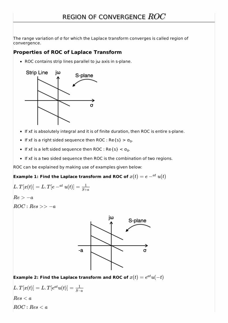
REGION OF CONVERGENCE REGION OF CONVERGENCE

The range variation of σ for which the Laplace transform converges is called region ofconvergence.

Properties of ROC of Laplace TransformROC contains strip lines parallel to jω axis in s-plane.

If x is absolutely integral and it is of finite duration, then ROC is entire s-plane.

If x is a right sided sequence then ROC : Re{s} > σo.

If x is a left sided sequence then ROC : Re{s} < σo.

If x is a two sided sequence then ROC is the combination of two regions.

ROC can be explained by making use of examples given below:

Example 1: Find the Laplace transform and ROC of

Example 2: Find the Laplace transform and ROC of

RROOCC

t

t

t

t

x(t) = e u(t)−at

L. T [x(t)] = L. T [e u(t)] =−at 1S+a

Re > −a

ROC : Res >> −a

x(t) = u(−t)eat

L. T [x(t)] = L. T [ u(t)] =eat 1S−a

Res < a

ROC : Res < a

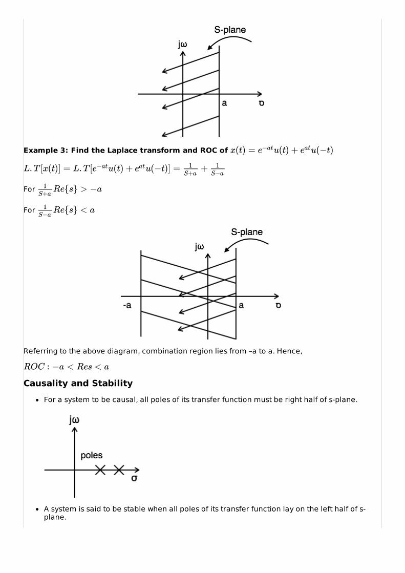
Example 3: Find the Laplace transform and ROC of

For

For

Referring to the above diagram, combination region lies from –a to a. Hence,

Causality and StabilityFor a system to be causal, all poles of its transfer function must be right half of s-plane.

A system is said to be stable when all poles of its transfer function lay on the left half of s-plane.

x(t) = u(t) + u(−t)e−at eat

L. T [x(t)] = L. T [ u(t) + u(−t)] = +e−at eat 1S+a

1S−a

Re{s} > −a1S+a

Re{s} < a1S−a

ROC : −a < Res < a

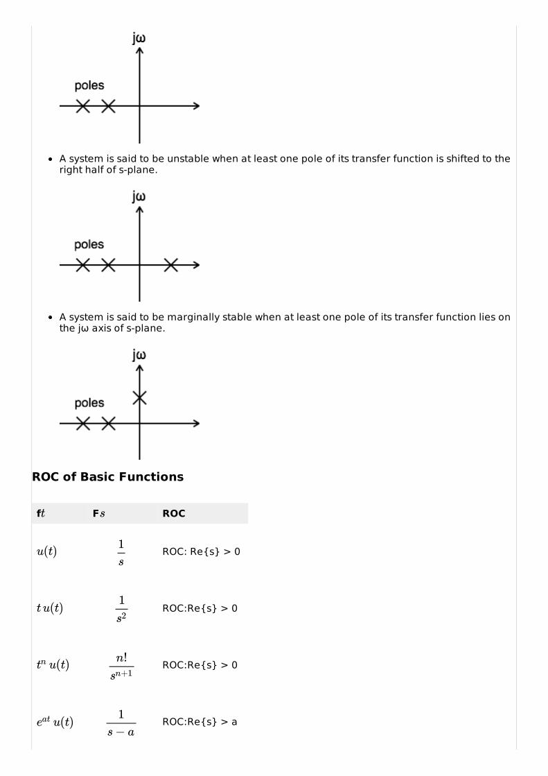
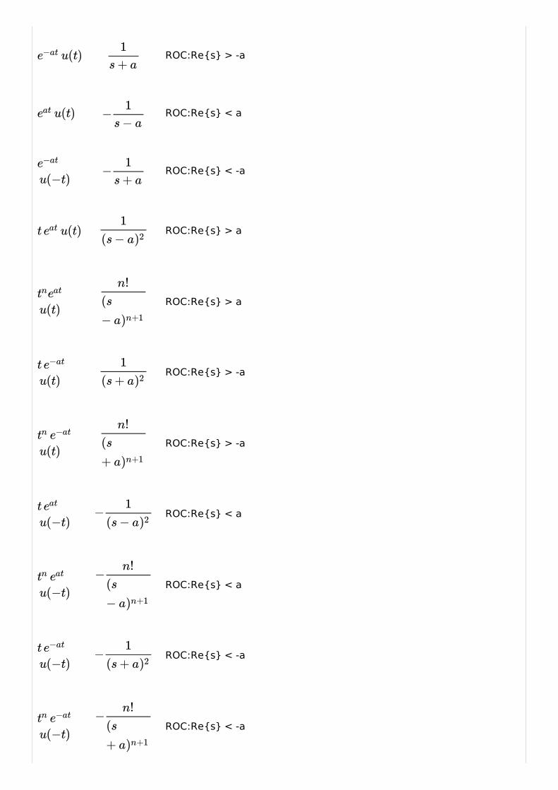
A system is said to be unstable when at least one pole of its transfer function is shifted to theright half of s-plane.

A system is said to be marginally stable when at least one pole of its transfer function lies onthe jω axis of s-plane.

ROC of Basic Functions

f F ROC

ROC: Re{s} > 0

ROC:Re{s} > 0

ROC:Re{s} > 0

ROC:Re{s} > a

t s

u(t) 1s

t u(t)1s2

u(t)tn n!sn+1

u(t)eat 1s − a

ROC:Re{s} > -a

ROC:Re{s} < a

ROC:Re{s} < -a

ROC:Re{s} > a

ROC:Re{s} > a

ROC:Re{s} > -a

ROC:Re{s} > -a

ROC:Re{s} < a

ROC:Re{s} < a

ROC:Re{s} < -a

ROC:Re{s} < -a

u(t)e−at 1s + a

u(t)eat −1

s − a

e−at

u(−t)−

1s + a

t u(t)eat1

(s − a)2

tneat

u(t)

n!(s

− a)n+1

t e−at

u(t)1

(s + a)2

tn e−at

u(t)

n!(s

+ a)n+1

t eat

u(−t)−

1(s − a)2

tn eat

u(−t)−

n!(s

− a)n+1

t e−at

u(−t)−

1(s + a)2

tn e−at

u(−t)−

n!(s

+ a)n+1

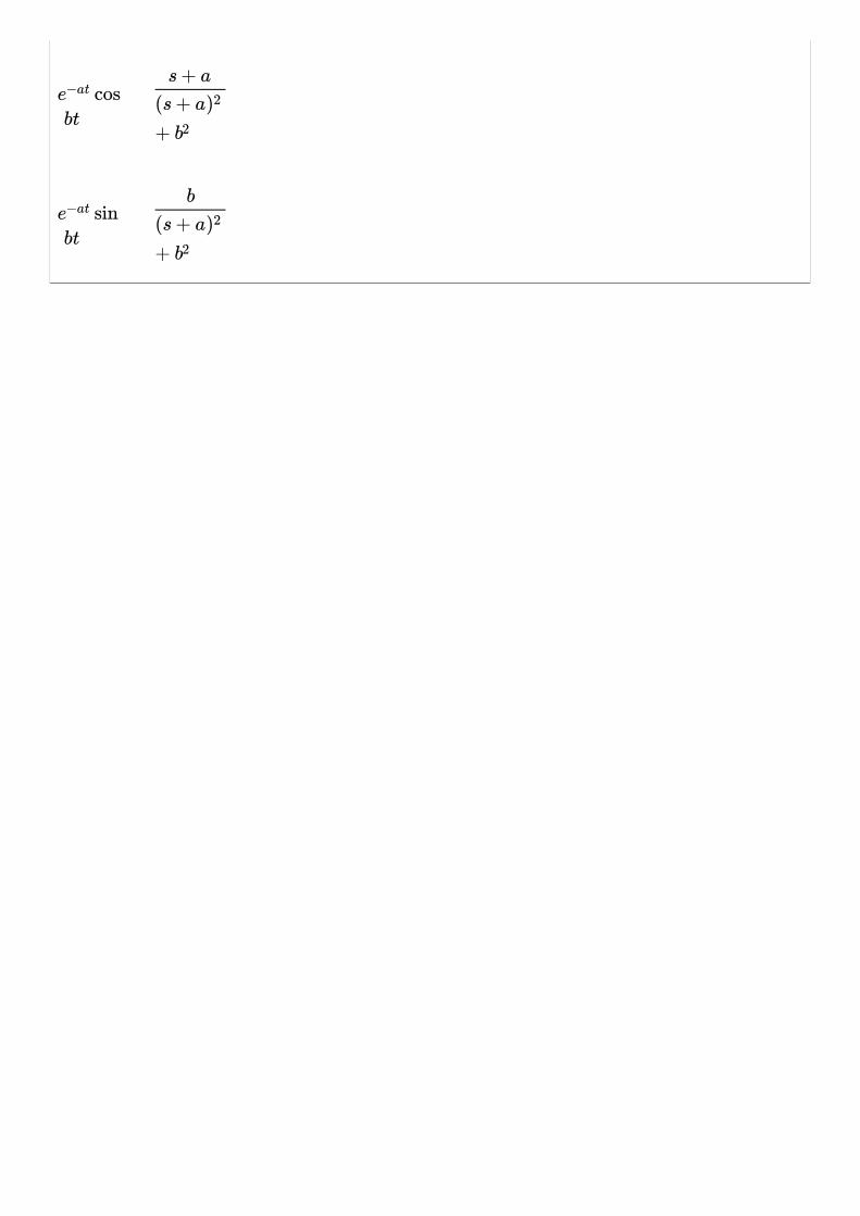
cose−at

bt

s + a

(s + a)2

+ b2

sine−at

bt

b

(s + a)2

+ b2

Z-TRANSFORMS Z-TRANSFORMS

Analysis of continuous time LTI systems can be done using z-transforms. It is a powerfulmathematical tool to convert differential equations into algebraic equations.

The bilateral z-transform of a discrete time signal x is given as

The unilateral z-transform of a discrete time signal x is given as

Z-transform may exist for some signals for which Discrete Time Fourier Transform doesnot exist.

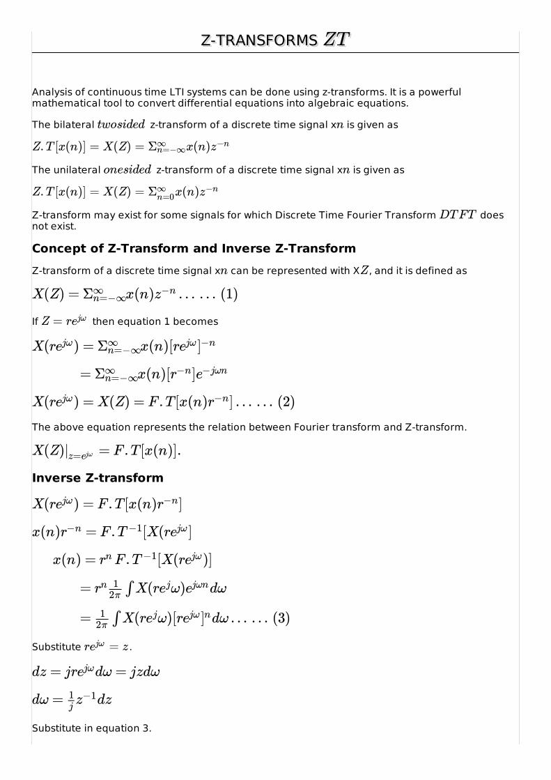
Concept of Z-Transform and Inverse Z-TransformZ-transform of a discrete time signal x can be represented with X , and it is defined as

If then equation 1 becomes

The above equation represents the relation between Fourier transform and Z-transform.

Inverse Z-transform

Substitute .

Substitute in equation 3.

ZZTT

twosided n

Z. T [x(n)] = X(Z) = x(n)Σ∞n=−∞ z−n

onesided n

Z. T [x(n)] = X(Z) = x(n)Σ∞n=0 z−n

DT FT

n Z

X(Z) = x(n) . . . . . . (1)Σ∞n=−∞ z−n

Z = rejω

X(r ) = x(n)[rejω Σ∞n=−∞ ejω ]−n

= x(n)[ ]Σ∞n=−∞ r−n e−jωn

X(r ) = X(Z) = F . T [x(n) ] . . . . . . (2)ejω r−n

X(Z) = F . T [x(n)].|z=ejω

X(r ) = F . T [x(n) ]ejω r−n

x(n) = F . [X(r ]r−n T −1 ejω

x(n) = F . [X(r )]rn T −1 ejω

= ∫ X(re ω) dωrn 12π

j ejωn

= ∫ X(re ω)[r dω . . . . . . (3)12π

j ejω ]n

r = zejω

dz = jr dω = jzdωejω

dω = dz1jz−1

3 → x(n) = ∫ X(z) dz = ∫ X(z) dz1 n 1 −1 1 n−1

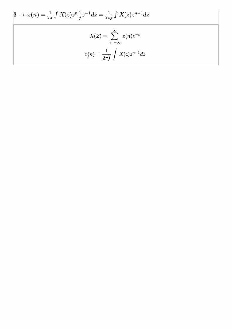
3 → x(n) = ∫ X(z) dz = ∫ X(z) dz12π

zn 1jz−1 1

2πjzn−1

X(Z) = x(n)∑n=−∞

∞

z−n

x(n) = ∫ X(z) dz1

2πjzn−1

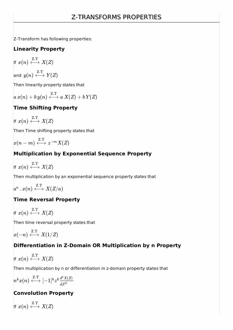
Z-TRANSFORMS PROPERTIESZ-TRANSFORMS PROPERTIES

Z-Transform has following properties:

Linearity Property

If

and

Then linearity property states that

Time Shifting Property

If

Then Time shifting property states that

Multiplication by Exponential Sequence Property

If

Then multiplication by an exponential sequence property states that

Time Reversal Property

If

Then time reversal property states that

Differentiation in Z-Domain OR Multiplication by n Property

If

Then multiplication by n or differentiation in z-domain property states that

Convolution Property

If

x(n) X(Z)⟷Z.T

y(n) Y (Z)⟷Z.T

a x(n) + b y(n) a X(Z) + b Y (Z)⟷Z.T

x(n) X(Z)⟷Z.T

x(n − m) X(Z)⟷Z.T

z−m

x(n) X(Z)⟷Z.T

. x(n) X(Z/a)an ⟷Z.T

x(n) X(Z)⟷Z.T

x(−n) X(1/Z)⟷Z.T

x(n) X(Z)⟷Z.T

x(n) [−1nk ⟷Z.T

]kzk X(Z)dk

dZK

x(n) X(Z)⟷Z.T

Z.T

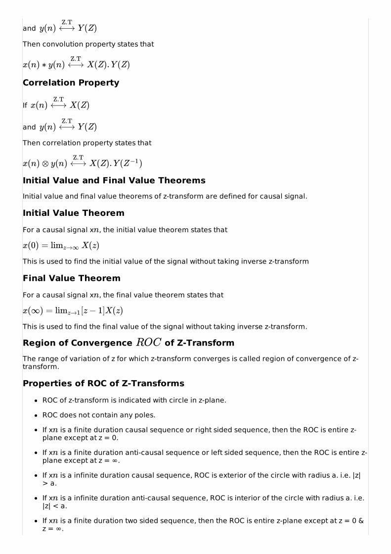
and

Then convolution property states that

Correlation Property

If

and

Then correlation property states that

Initial Value and Final Value TheoremsInitial value and final value theorems of z-transform are defined for causal signal.

Initial Value TheoremFor a causal signal x , the initial value theorem states that

This is used to find the initial value of the signal without taking inverse z-transform

Final Value TheoremFor a causal signal x , the final value theorem states that

This is used to find the final value of the signal without taking inverse z-transform.

Region of Convergence of Z-TransformThe range of variation of z for which z-transform converges is called region of convergence of z-transform.

Properties of ROC of Z-TransformsROC of z-transform is indicated with circle in z-plane.

ROC does not contain any poles.

If x is a finite duration causal sequence or right sided sequence, then the ROC is entire z-plane except at z = 0.

If x is a finite duration anti-causal sequence or left sided sequence, then the ROC is entire z-plane except at z = ∞.

If x is a infinite duration causal sequence, ROC is exterior of the circle with radius a. i.e. |z|> a.

If x is a infinite duration anti-causal sequence, ROC is interior of the circle with radius a. i.e.|z| < a.

If x is a finite duration two sided sequence, then the ROC is entire z-plane except at z = 0 &z = ∞.

y(n) Y (Z)⟷Z.T

x(n) ∗ y(n) X(Z). Y (Z)⟷Z.T

x(n) X(Z)⟷Z.T

y(n) Y (Z)⟷Z.T

x(n) ⊗ y(n) X(Z). Y ( )⟷Z.T

Z−1

n

x(0) = X(z)limz→∞

n

x(∞) = [z − 1]X(z)limz→1

ROC

n

n

n

n

n

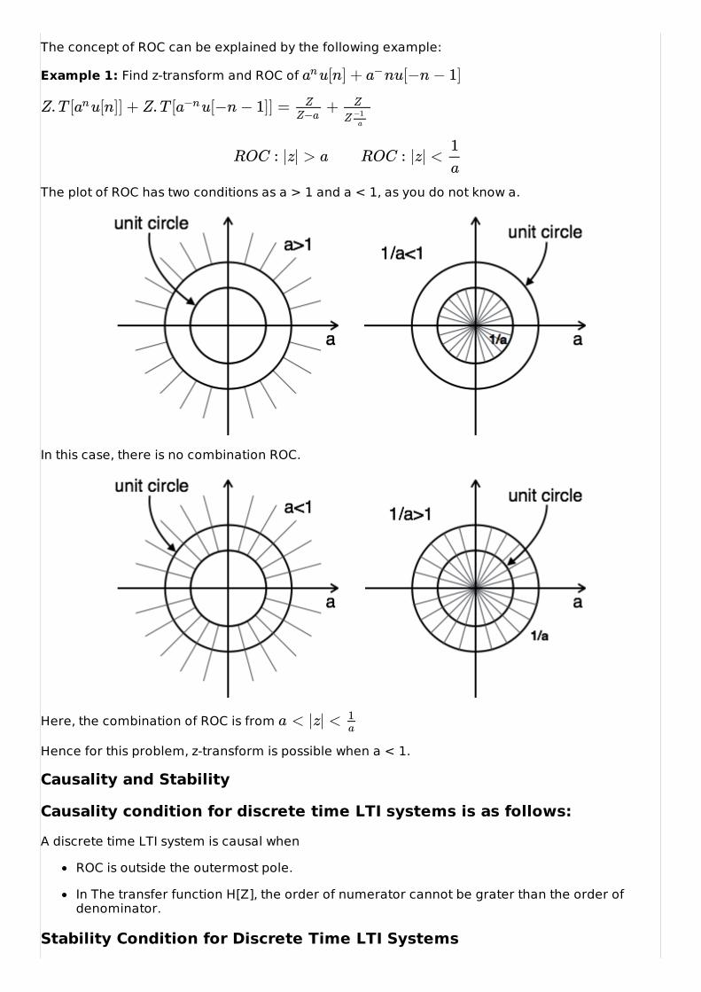
The concept of ROC can be explained by the following example:

Example 1: Find z-transform and ROC of

The plot of ROC has two conditions as a > 1 and a < 1, as you do not know a.

In this case, there is no combination ROC.

Here, the combination of ROC is from

Hence for this problem, z-transform is possible when a < 1.

Causality and Stability

Causality condition for discrete time LTI systems is as follows:A discrete time LTI system is causal when

ROC is outside the outermost pole.

In The transfer function H[Z], the order of numerator cannot be grater than the order ofdenominator.

Stability Condition for Discrete Time LTI Systems

u[n] + nu[−n − 1]an a−

Z. T [ u[n]] + Z. T [ u[−n − 1]] = +an a−n ZZ−a

Z

Z −1a

ROC : |z| > a ROC : |z| <1a

a < |z| < 1a

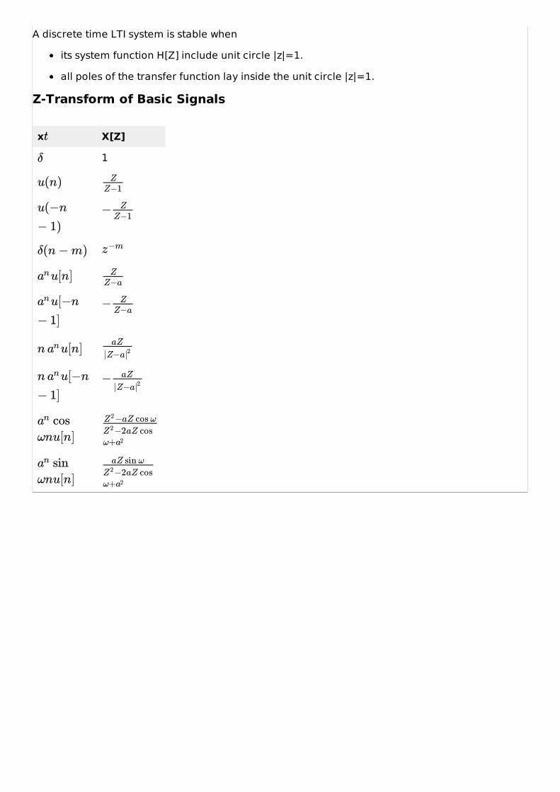
A discrete time LTI system is stable when

its system function H[Z] include unit circle |z|=1.

all poles of the transfer function lay inside the unit circle |z|=1.

Z-Transform of Basic Signals

x X[Z]

1

t

δ

u(n) ZZ−1

u(−n

− 1)− Z

Z−1

δ(n − m) z−m

u[n]an ZZ−a

u[−nan

− 1]− Z

Z−a

n u[n]an aZ

|Z−a|2

n u[−nan

− 1]− aZ

|Z−a|2

cosan

ωnu[n]

−aZ cos ωZ2

−2aZ cosZ2

ω+a2

sinan

ωnu[n]

aZ sin ω

−2aZ cosZ2

ω+a2