Chapter 3 Data and Signals - CSE IIT Kgp

3.1

Chapter 3

Data and Signals

Copyright © The McGraw-Hill Companies, Inc. Permission required for reproduction or display.

3.2

To be transmitted, data must be transformed to electromagnetic signals.

Note

3.3

3-1 ANALOG AND DIGITAL

Data can be analog or digital. The term analog data refers to information that is continuous; digital data refers to information that has discrete states. Analog data take on continuous values. Digital data take on discrete values.

Analog and Digital Data Analog and Digital Signals Periodic and Nonperiodic Signals

Topics discussed in this section:

3.4

Note

Data can be analog or digital. Analog data are continuous and take

continuous values. Digital data have discrete states and

take discrete values.

3.5

Signals can be analog or digital. Analog signals can have an infinite number of values in a range; digital

signals can have only a limited number of values.

Note

3.6

Figure 3.1 Comparison of analog and digital signals

3.7

In data communications, we commonly use periodic analog signals and

nonperiodic digital signals.

Note

3.8

3-2 PERIODIC ANALOG SIGNALS

Periodic analog signals can be classified as simple or composite. A simple periodic analog signal, a sine wave, cannot be decomposed into simpler signals. A composite periodic analog signal is composed of multiple sine waves.

Sine Wave Wavelength Time and Frequency Domain Composite Signals Bandwidth


3.9

Figure 3.2 A sine wave

3.10

We discuss a mathematical approach to sine waves in Appendix C.

Note

3.11

The power in your house can be represented by a sine wave with a peak amplitude of 155 to 170 V. However, it is common knowledge that the voltage of the power in U.S. homes is 110 to 120 V. This discrepancy is due to the fact that these are root mean square (rms) values. The signal is squared and then the average amplitude is calculated. The peak value is equal to 2½ × rms value.

Example 3.1

3.12

Figure 3.3 Two signals with the same phase and frequency, but different amplitudes

3.13

The voltage of a battery is a constant; this constant value can be considered a sine wave, as we will see later. For example, the peak value of an AA battery is normally 1.5 V.

Example 3.2

3.14

Frequency and period are the inverse of each other.

Note

3.15

Figure 3.4 Two signals with the same amplitude and phase, but different frequencies

3.16

Table 3.1 Units of period and frequency

3.17

The power we use at home has a frequency of 60 Hz. The period of this sine wave can be determined as follows:

Example 3.3

3.18

Express a period of 100 ms in microseconds.

Example 3.4

Solution From Table 3.1 we find the equivalents of 1 ms (1 ms is 10−3 s) and 1 s (1 s is 106 μs). We make the following substitutions:.

3.19

The period of a signal is 100 ms. What is its frequency in kilohertz?

Example 3.5

Solution First we change 100 ms to seconds, and then we calculate the frequency from the period (1 Hz = 10−3 kHz).

3.20

Frequency is the rate of change with respect to time.

Change in a short span of time

means high frequency.

Change over a long span of time means low frequency.

Note

3.21

If a signal does not change at all, its frequency is zero.

If a signal changes instantaneously, its frequency is infinite.

Note

3.22

Phase describes the position of the waveform relative to time 0.

Note

3.23

Figure 3.5 Three sine waves with the same amplitude and frequency, but different phases

3.24

A sine wave is offset 1/6 cycle with respect to time 0. What is its phase in degrees and radians?

Example 3.6

Solution We know that 1 complete cycle is 360°. Therefore, 1/6 cycle is

3.25

Figure 3.6 Wavelength and period

3.26

Figure 3.7 The time-domain and frequency-domain plots of a sine wave

3.27

A complete sine wave in the time domain can be represented by one

single spike in the frequency domain.

Note

3.28

The frequency domain is more compact and useful when we are dealing with more than one sine wave. For example, Figure 3.8 shows three sine waves, each with different amplitude and frequency. All can be represented by three spikes in the frequency domain.

Example 3.7

3.29

Figure 3.8 The time domain and frequency domain of three sine waves

3.30

A single-frequency sine wave is not useful in data communications;

we need to send a composite signal, a signal made of many simple sine waves.

Note

3.31

According to Fourier analysis, any composite signal is a combination of

simple sine waves with different frequencies, amplitudes, and phases.

Fourier analysis is discussed in Appendix C.

Note

3.32

If the composite signal is periodic, the decomposition gives a series of signals

with discrete frequencies; if the composite signal is nonperiodic, the decomposition gives a combination

of sine waves with continuous frequencies.

Note

3.33

Figure 3.9 shows a periodic composite signal with frequency f. This type of signal is not typical of those found in data communications. We can consider it to be three alarm systems, each with a different frequency. The analysis of this signal can give us a good understanding of how to decompose signals.

Example 3.8

3.34

Figure 3.9 A composite periodic signal

3.35

Figure 3.10 Decomposition of a composite periodic signal in the time and frequency domains

3.36

Figure 3.11 shows a nonperiodic composite signal. It can be the signal created by a microphone or a telephone set when a word or two is pronounced. In this case, the composite signal cannot be periodic, because that implies that we are repeating the same word or words with exactly the same tone.

Example 3.9

3.37

Figure 3.11 The time and frequency domains of a nonperiodic signal

3.38

The bandwidth of a composite signal is the difference between the

highest and the lowest frequencies contained in that signal.

Note

3.39

Figure 3.12 The bandwidth of periodic and nonperiodic composite signals

3.40

If a periodic signal is decomposed into five sine waves with frequencies of 100, 300, 500, 700, and 900 Hz, what is its bandwidth? Draw the spectrum, assuming all components have a maximum amplitude of 10 V. Solution Let fh be the highest frequency, fl the lowest frequency, and B the bandwidth. Then

Example 3.10

The spectrum has only five spikes, at 100, 300, 500, 700, and 900 Hz (see Figure 3.13).

3.41

Figure 3.13 The bandwidth for Example 3.10

3.42

A periodic signal has a bandwidth of 20 Hz. The highest frequency is 60 Hz. What is the lowest frequency? Draw the spectrum if the signal contains all frequencies of the same amplitude. Solution Let fh be the highest frequency, fl the lowest frequency, and B the bandwidth. Then

Example 3.11

The spectrum contains all integer frequencies. We show this by a series of spikes (see Figure 3.14).

3.43


3.44

A nonperiodic composite signal has a bandwidth of 200 kHz, with a middle frequency of 140 kHz and peak amplitude of 20 V. The two extreme frequencies have an amplitude of 0. Draw the frequency domain of the signal. Solution The lowest frequency must be at 40 kHz and the highest at 240 kHz. Figure 3.15 shows the frequency domain and the bandwidth.

Example 3.12

3.45


3.46

An example of a nonperiodic composite signal is the signal propagated by an AM radio station. In the United States, each AM radio station is assigned a 10-kHz bandwidth. The total bandwidth dedicated to AM radio ranges from 530 to 1700 kHz. We will show the rationale behind this 10-kHz bandwidth in Chapter 5.

Example 3.13

3.47

Another example of a nonperiodic composite signal is the signal propagated by an FM radio station. In the United States, each FM radio station is assigned a 200-kHz bandwidth. The total bandwidth dedicated to FM radio ranges from 88 to 108 MHz. We will show the rationale behind this 200-kHz bandwidth in Chapter 5.

Example 3.14

3.48

Another example of a nonperiodic composite signal is the signal received by an old-fashioned analog black-and-white TV. A TV screen is made up of pixels. If we assume a resolution of 525 × 700, we have 367,500 pixels per screen. If we scan the screen 30 times per second, this is 367,500 × 30 = 11,025,000 pixels per second. The worst-case scenario is alternating black and white pixels. We can send 2 pixels per cycle. Therefore, we need 11,025,000 / 2 = 5,512,500 cycles per second, or Hz. The bandwidth needed is 5.5125 MHz.

Example 3.15

3.49

3-3 DIGITAL SIGNALS

In addition to being represented by an analog signal, information can also be represented by a digital signal. For example, a 1 can be encoded as a positive voltage and a 0 as zero voltage. A digital signal can have more than two levels. In this case, we can send more than 1 bit for each level.

Bit Rate Bit Length Digital Signal as a Composite Analog Signal Application Layer


3.50

Figure 3.16 Two digital signals: one with two signal levels and the other with four signal levels

3.51

Appendix C reviews information about exponential and logarithmic functions.

Note

Appendix C reviews information about exponential and logarithmic functions.

3.52

A digital signal has eight levels. How many bits are needed per level? We calculate the number of bits from the formula

Example 3.16

Each signal level is represented by 3 bits.

3.53

A digital signal has nine levels. How many bits are needed per level? We calculate the number of bits by using the formula. Each signal level is represented by 3.17 bits. However, this answer is not realistic. The number of bits sent per level needs to be an integer as well as a power of 2. For this example, 4 bits can represent one level.

Example 3.17

3.54

Assume we need to download text documents at the rate of 100 pages per minute. What is the required bit rate of the channel? Solution A page is an average of 24 lines with 80 characters in each line. If we assume that one character requires 8 bits, the bit rate is

Example 3.18

3.55

A digitized voice channel, as we will see in Chapter 4, is made by digitizing a 4-kHz bandwidth analog voice signal. We need to sample the signal at twice the highest frequency (two samples per hertz). We assume that each sample requires 8 bits. What is the required bit rate? Solution The bit rate can be calculated as

Example 3.19

3.56

What is the bit rate for high-definition TV (HDTV)? Solution HDTV uses digital signals to broadcast high quality video signals. The HDTV screen is normally a ratio of 16 : 9. There are 1920 by 1080 pixels per screen, and the screen is renewed 30 times per second. Twenty-four bits represents one color pixel.

Example 3.20

The TV stations reduce this rate to 20 to 40 Mbps through compression.

3.57

Figure 3.17 The time and frequency domains of periodic and nonperiodic digital signals

3.58

Figure 3.18 Baseband transmission

3.59

A digital signal is a composite analog signal with an infinite bandwidth.

Note

3.60

Figure 3.19 Bandwidths of two low-pass channels

3.61

Figure 3.20 Baseband transmission using a dedicated medium

3.62

Baseband transmission of a digital signal that preserves the shape of the

digital signal is possible only if we have a low-pass channel with an infinite or

very wide bandwidth.

Note

3.63

An example of a dedicated channel where the entire bandwidth of the medium is used as one single channel is a LAN. Almost every wired LAN today uses a dedicated channel for two stations communicating with each other. In a bus topology LAN with multipoint connections, only two stations can communicate with each other at each moment in time (timesharing); the other stations need to refrain from sending data. In a star topology LAN, the entire channel between each station and the hub is used for communication between these two entities. We study LANs in Chapter 14.

Example 3.21

3.64

Figure 3.21 Rough approximation of a digital signal using the first harmonic for worst case

3.65

Figure 3.22 Simulating a digital signal with first three harmonics

3.66

In baseband transmission, the required bandwidth is proportional to the bit rate;

if we need to send bits faster, we need more bandwidth.

Note

In baseband transmission, the required bandwidth is proportional to the bit rate; if we need to send bits faster, we need

more bandwidth.

3.67

Table 3.2 Bandwidth requirements

3.68

What is the required bandwidth of a low-pass channel if we need to send 1 Mbps by using baseband transmission? Solution The answer depends on the accuracy desired. a. The minimum bandwidth, is B = bit rate /2, or 500 kHz. b. A better solution is to use the first and the third harmonics with B = 3 × 500 kHz = 1.5 MHz. c. Still a better solution is to use the first, third, and fifth harmonics with B = 5 × 500 kHz = 2.5 MHz.

Example 3.22

3.69

We have a low-pass channel with bandwidth 100 kHz. What is the maximum bit rate of this

channel? Solution The maximum bit rate can be achieved if we use the first harmonic. The bit rate is 2 times the available bandwidth, or 200 kbps.

Example 3.22

3.70

Figure 3.23 Bandwidth of a bandpass channel

3.71

If the available channel is a bandpass channel, we cannot send the digital

signal directly to the channel; we need to convert the digital signal to an analog signal before transmission.

Note

3.72

Figure 3.24 Modulation of a digital signal for transmission on a bandpass channel

3.73

An example of broadband transmission using modulation is the sending of computer data through a telephone subscriber line, the line connecting a resident to the central telephone office. These lines are designed to carry voice with a limited bandwidth. The channel is considered a bandpass channel. We convert the digital signal from the computer to an analog signal, and send the analog signal. We can install two converters to change the digital signal to analog and vice versa at the receiving end. The converter, in this case, is called a modem which we discuss in detail in Chapter 5.

Example 3.24

3.74

A second example is the digital cellular telephone. For better reception, digital cellular phones convert the analog voice signal to a digital signal (see Chapter 16). Although the bandwidth allocated to a company providing digital cellular phone service is very wide, we still cannot send the digital signal without conversion. The reason is that we only have a bandpass channel available between caller and callee. We need to convert the digitized voice to a composite analog signal before sending.

Example 3.25

3.75

3-4 TRANSMISSION IMPAIRMENT

Signals travel through transmission media, which are not perfect. The imperfection causes signal impairment. This means that the signal at the beginning of the medium is not the same as the signal at the end of the medium. What is sent is not what is received. Three causes of impairment are attenuation, distortion, and noise.

Attenuation Distortion Noise


3.76

Figure 3.25 Causes of impairment

3.77

Figure 3.26 Attenuation

3.78

Suppose a signal travels through a transmission medium and its power is reduced to one-half. This means that P2 is (1/2)P1. In this case, the attenuation (loss of power) can be calculated as

Example 3.26

A loss of 3 dB (–3 dB) is equivalent to losing one-half the power.

3.79

A signal travels through an amplifier, and its power is increased 10 times. This means that P2 = 10P1 . In this case, the amplification (gain of power) can be calculated as

Example 3.27

3.80

One reason that engineers use the decibel to measure the changes in the strength of a signal is that decibel numbers can be added (or subtracted) when we are measuring several points (cascading) instead of just two. In Figure 3.27 a signal travels from point 1 to point 4. In this case, the decibel value can be calculated as

Example 3.28

3.81

Figure 3.27 Decibels for Example 3.28

3.82

Sometimes the decibel is used to measure signal power in milliwatts. In this case, it is referred to as dBm and is calculated as dBm = 10 log10 Pm , where Pm is the power in milliwatts. Calculate the power of a signal with dBm = −30. Solution We can calculate the power in the signal as

Example 3.29

3.83

The loss in a cable is usually defined in decibels per kilometer (dB/km). If the signal at the beginning of a cable with −0.3 dB/km has a power of 2 mW, what is the power of the signal at 5 km? Solution The loss in the cable in decibels is 5 × (−0.3) = −1.5 dB. We can calculate the power as

Example 3.30

3.84

Figure 3.28 Distortion

3.85

Figure 3.29 Noise

3.86

The power of a signal is 10 mW and the power of the noise is 1 μW; what are the values of SNR and SNRdB ? Solution The values of SNR and SNRdB can be calculated as follows:

Example 3.31

3.87

The values of SNR and SNRdB for a noiseless channel are

Example 3.32

We can never achieve this ratio in real life; it is an ideal.

3.88

Figure 3.30 Two cases of SNR: a high SNR and a low SNR

3.89

3-5 DATA RATE LIMITS

A very important consideration in data communications is how fast we can send data, in bits per second, over a channel. Data rate depends on three factors: 1. The bandwidth available 2. The level of the signals we use 3. The quality of the channel (the level of noise)

Noiseless Channel: Nyquist Bit Rate Noisy Channel: Shannon Capacity Using Both Limits


3.90

Increasing the levels of a signal may reduce the reliability of the system.

Note

3.91

Does the Nyquist theorem bit rate agree with the intuitive bit rate described in baseband transmission? Solution They match when we have only two levels. We said, in baseband transmission, the bit rate is 2 times the bandwidth if we use only the first harmonic in the worst case. However, the Nyquist formula is more general than what we derived intuitively; it can be applied to baseband transmission and modulation. Also, it can be applied when we have two or more levels of signals.

Example 3.33

3.92

Consider a noiseless channel with a bandwidth of 3000 Hz transmitting a signal with two signal levels. The maximum bit rate can be calculated as

Example 3.34

3.93

Consider the same noiseless channel transmitting a signal with four signal levels (for each level, we send 2 bits). The maximum bit rate can be calculated as

Example 3.35

3.94

We need to send 265 kbps over a noiseless channel with a bandwidth of 20 kHz. How many signal levels do we need? Solution We can use the Nyquist formula as shown:

Example 3.36

Since this result is not a power of 2, we need to either increase the number of levels or reduce the bit rate. If we have 128 levels, the bit rate is 280 kbps. If we have 64 levels, the bit rate is 240 kbps.

3.95

Consider an extremely noisy channel in which the value of the signal-to-noise ratio is almost zero. In other words, the noise is so strong that the signal is faint. For this channel the capacity C is calculated as

Example 3.37

This means that the capacity of this channel is zero regardless of the bandwidth. In other words, we cannot receive any data through this channel.

3.96

We can calculate the theoretical highest bit rate of a regular telephone line. A telephone line normally has a bandwidth of 3000. The signal-to-noise ratio is usually 3162. For this channel the capacity is calculated as

Example 3.38

This means that the highest bit rate for a telephone line is 34.860 kbps. If we want to send data faster than this, we can either increase the bandwidth of the line or improve the signal-to-noise ratio.

3.97

The signal-to-noise ratio is often given in decibels. Assume that SNRdB = 36 and the channel bandwidth is 2 MHz. The theoretical channel capacity can be calculated as

Example 3.39

3.98

For practical purposes, when the SNR is very high, we can assume that SNR + 1 is almost the same as SNR. In these cases, the theoretical channel capacity can be simplified to

Example 3.40

For example, we can calculate the theoretical capacity of the previous example as

3.99

We have a channel with a 1-MHz bandwidth. The SNR for this channel is 63. What are the appropriate bit rate and signal level? Solution First, we use the Shannon formula to find the upper limit.

Example 3.41

3.100

The Shannon formula gives us 6 Mbps, the upper limit. For better performance we choose something lower, 4 Mbps, for example. Then we use the Nyquist formula to find the number of signal levels.

Example 3.41 (continued)

3.101

The Shannon capacity gives us the upper limit; the Nyquist formula tells us

how many signal levels we need.

Note

3.102

3-6 PERFORMANCE

One important issue in networking is the performance of the network—how good is it? We discuss quality of service, an overall measurement of network performance, in greater detail in Chapter 24. In this section, we introduce terms that we need for future chapters.

Bandwidth Throughput Latency (Delay) Bandwidth-Delay Product


3.103

In networking, we use the term bandwidth in two contexts.

❏ The first, bandwidth in hertz, refers to the range of frequencies in a composite signal or the range of frequencies that a channel can pass. ❏ The second, bandwidth in bits per second, refers to the speed of bit transmission in a channel or link.

Note

3.104

The bandwidth of a subscriber line is 4 kHz for voice or data. The bandwidth of this line for data transmission can be up to 56,000 bps using a sophisticated modem to change the digital signal to analog.

Example 3.42

3.105

If the telephone company improves the quality of the line and increases the bandwidth to 8 kHz, we can send 112,000 bps by using the same technology as mentioned in Example 3.42.

Example 3.43

3.106

A network with bandwidth of 10 Mbps can pass only an average of 12,000 frames per minute with each frame carrying an average of 10,000 bits. What is the throughput of this network? Solution We can calculate the throughput as

Example 3.44

The throughput is almost one-fifth of the bandwidth in this case.

3.107

What is the propagation time if the distance between the two points is 12,000 km? Assume the propagation speed to be 2.4 × 108 m/s in cable. Solution We can calculate the propagation time as

Example 3.45

The example shows that a bit can go over the Atlantic Ocean in only 50 ms if there is a direct cable between the source and the destination.

3.108

What are the propagation time and the transmission time for a 2.5-kbyte message (an e-mail) if the bandwidth of the network is 1 Gbps? Assume that the distance between the sender and the receiver is 12,000 km and that light travels at 2.4 × 108 m/s. Solution We can calculate the propagation and transmission time as shown on the next slide:

Example 3.46

3.109

Note that in this case, because the message is short and the bandwidth is high, the dominant factor is the propagation time, not the transmission time. The transmission time can be ignored.


3.110

What are the propagation time and the transmission time for a 5-Mbyte message (an image) if the bandwidth of the network is 1 Mbps? Assume that the distance between the sender and the receiver is 12,000 km and that light travels at 2.4 × 108 m/s. Solution We can calculate the propagation and transmission times as shown on the next slide.

Example 3.47

3.111

Note that in this case, because the message is very long and the bandwidth is not very high, the dominant factor is the transmission time, not the propagation time. The propagation time can be ignored.


3.112

Figure 3.31 Filling the link with bits for case 1

3.113

We can think about the link between two points as a pipe. The cross section of the pipe represents the bandwidth, and the length of the pipe represents the delay. We can say the volume of the pipe defines the bandwidth-delay product, as shown in Figure 3.33.

Example 3.48

3.114

Figure 3.32 Filling the link with bits in case 2

3.115

The bandwidth-delay product defines the number of bits that can fill the link.

Note

3.116

Figure 3.33 Concept of bandwidth-delay product

4.1

Chapter 4

Digital Transmission


4.2

4-1 DIGITAL-TO-DIGITAL CONVERSION

In this section, we see how we can represent digital data by using digital signals. The conversion involves three techniques: line coding, block coding, and scrambling. Line coding is always needed; block coding and scrambling may or may not be needed.

Line Coding Line Coding Schemes Block Coding Scrambling


4.3

Figure 4.1 Line coding and decoding

4.4

Figure 4.2 Signal element versus data element

4.5

A signal is carrying data in which one data element is encoded as one signal element ( r = 1). If the bit rate is 100 kbps, what is the average value of the baud rate if c is between 0 and 1?

Solution We assume that the average value of c is 1/2 . The baud rate is then

Example 4.1

4.6

Although the actual bandwidth of a digital signal is infinite, the effective

bandwidth is finite.

Note

4.7

The maximum data rate of a channel (see Chapter 3) is Nmax = 2 × B × log2 L (defined by the Nyquist formula). Does this agree with the previous formula for Nmax?

Solution A signal with L levels actually can carry log2L bits per level. If each level corresponds to one signal element and we assume the average case (c = 1/2), then we have

Example 4.2

4.8

Figure 4.3 Effect of lack of synchronization

4.9

In a digital transmission, the receiver clock is 0.1 percent faster than the sender clock. How many extra bits per second does the receiver receive if the data rate is 1 kbps? How many if the data rate is 1 Mbps? Solution At 1 kbps, the receiver receives 1001 bps instead of 1000 bps.

Example 4.3

At 1 Mbps, the receiver receives 1,001,000 bps instead of 1,000,000 bps.

4.10

Figure 4.4 Line coding schemes

4.11

Figure 4.5 Unipolar NRZ scheme

4.12

Figure 4.6 Polar NRZ-L and NRZ-I schemes

4.13

In NRZ-L the level of the voltage determines the value of the bit.

In NRZ-I the inversion or the lack of inversion

determines the value of the bit.

Note

4.14

NRZ-L and NRZ-I both have an average signal rate of N/2 Bd.

Note

4.15

NRZ-L and NRZ-I both have a DC component problem.

Note

4.16

A system is using NRZ-I to transfer 10-Mbps data. What are the average signal rate and minimum bandwidth?

Solution The average signal rate is S = N/2 = 500 kbaud. The minimum bandwidth for this average baud rate is Bmin = S = 500 kHz.

Example 4.4

4.17

Figure 4.7 Polar RZ scheme

4.18

Figure 4.8 Polar biphase: Manchester and differential Manchester schemes

4.19

In Manchester and differential Manchester encoding, the transition

at the middle of the bit is used for synchronization.

Note

4.20

The minimum bandwidth of Manchester and differential Manchester is 2 times

that of NRZ.

Note

4.21

In bipolar encoding, we use three levels: positive, zero, and negative.

Note

4.22

Figure 4.9 Bipolar schemes: AMI and pseudoternary

4.23

In mBnL schemes, a pattern of m data elements is encoded as a pattern of n

signal elements in which 2m ≤ Ln.

Note

4.24

Figure 4.10 Multilevel: 2B1Q scheme

4.25

Figure 4.11 Multilevel: 8B6T scheme

4.26

Figure 4.12 Multilevel: 4D-PAM5 scheme

4.27

Figure 4.13 Multitransition: MLT-3 scheme

4.28

Table 4.1 Summary of line coding schemes

4.29

Block coding is normally referred to as mB/nB coding;

it replaces each m-bit group with an n-bit group.

Note

4.30

Figure 4.14 Block coding concept

4.31

Figure 4.15 Using block coding 4B/5B with NRZ-I line coding scheme

4.32

Table 4.2 4B/5B mapping codes

4.33

Figure 4.16 Substitution in 4B/5B block coding

4.34

We need to send data at a 1-Mbps rate. What is the minimum required bandwidth, using a combination of 4B/5B and NRZ-I or Manchester coding?

Solution First 4B/5B block coding increases the bit rate to 1.25 Mbps. The minimum bandwidth using NRZ-I is N/2 or 625 kHz. The Manchester scheme needs a minimum bandwidth of 1 MHz. The first choice needs a lower bandwidth, but has a DC component problem; the second choice needs a higher bandwidth, but does not have a DC component problem.

Example 4.5

4.35

Figure 4.17 8B/10B block encoding

4.36

Figure 4.18 AMI used with scrambling

4.37

Figure 4.19 Two cases of B8ZS scrambling technique

4.38

B8ZS substitutes eight consecutive zeros with 000VB0VB.

Note

4.39

Figure 4.20 Different situations in HDB3 scrambling technique

4.40

HDB3 substitutes four consecutive zeros with 000V or B00V depending

on the number of nonzero pulses after the last substitution.

Note

4.41

4-2 ANALOG-TO-DIGITAL CONVERSION

We have seen in Chapter 3 that a digital signal is superior to an analog signal. The tendency today is to change an analog signal to digital data. In this section we describe two techniques, pulse code modulation and delta modulation.

Pulse Code Modulation (PCM) Delta Modulation (DM)


4.42

Figure 4.21 Components of PCM encoder

4.43

Figure 4.22 Three different sampling methods for PCM

4.44

According to the Nyquist theorem, the sampling rate must be

at least 2 times the highest frequency contained in the signal.

Note

4.45

Figure 4.23 Nyquist sampling rate for low-pass and bandpass signals

4.46

For an intuitive example of the Nyquist theorem, let us sample a simple sine wave at three sampling rates: fs = 4f (2 times the Nyquist rate), fs = 2f (Nyquist rate), and fs = f (one-half the Nyquist rate). Figure 4.24 shows the sampling and the subsequent recovery of the signal. It can be seen that sampling at the Nyquist rate can create a good approximation of the original sine wave (part a). Oversampling in part b can also create the same approximation, but it is redundant and unnecessary. Sampling below the Nyquist rate (part c) does not produce a signal that looks like the original sine wave.

Example 4.6

4.47

Figure 4.24 Recovery of a sampled sine wave for different sampling rates

4.48

Consider the revolution of a hand of a clock. The second hand of a clock has a period of 60 s. According to the Nyquist theorem, we need to sample the hand every 30 s (Ts = T or fs = 2f ). In Figure 4.25a, the sample points, in order, are 12, 6, 12, 6, 12, and 6. The receiver of the samples cannot tell if the clock is moving forward or backward. In part b, we sample at double the Nyquist rate (every 15 s). The sample points are 12, 3, 6, 9, and 12. The clock is moving forward. In part c, we sample below the Nyquist rate (Ts = T or fs = f ). The sample points are 12, 9, 6, 3, and 12. Although the clock is moving forward, the receiver thinks that the clock is moving backward.

Example 4.7

4.49

Figure 4.25 Sampling of a clock with only one hand

4.50

An example related to Example 4.7 is the seemingly backward rotation of the wheels of a forward-moving car in a movie. This can be explained by under-sampling. A movie is filmed at 24 frames per second. If a wheel is rotating more than 12 times per second, the under-sampling creates the impression of a backward rotation.

Example 4.8

4.51

Telephone companies digitize voice by assuming a maximum frequency of 4000 Hz. The sampling rate therefore is 8000 samples per second.

Example 4.9

4.52

A complex low-pass signal has a bandwidth of 200 kHz. What is the minimum sampling rate for this signal?

Solution The bandwidth of a low-pass signal is between 0 and f, where f is the maximum frequency in the signal. Therefore, we can sample this signal at 2 times the highest frequency (200 kHz). The sampling rate is therefore 400,000 samples per second.

Example 4.10

4.53

A complex bandpass signal has a bandwidth of 200 kHz. What is the minimum sampling rate for this signal?

Solution We cannot find the minimum sampling rate in this case because we do not know where the bandwidth starts or ends. We do not know the maximum frequency in the signal.

Example 4.11

4.54

Figure 4.26 Quantization and encoding of a sampled signal

4.55

What is the SNRdB in the example of Figure 4.26?

Solution We can use the formula to find the quantization. We have eight levels and 3 bits per sample, so

SNRdB = 6.02(3) + 1.76 = 19.82 dB

Increasing the number of levels increases the SNR.

Example 4.12

4.56

A telephone subscriber line must have an SNRdB above 40. What is the minimum number of bits per sample?

Solution We can calculate the number of bits as

Example 4.13

Telephone companies usually assign 7 or 8 bits per sample.

4.57

We want to digitize the human voice. What is the bit rate, assuming 8 bits per sample?

Solution The human voice normally contains frequencies from 0 to 4000 Hz. So the sampling rate and bit rate are calculated as follows:

Example 4.14

4.58

Figure 4.27 Components of a PCM decoder

4.59

We have a low-pass analog signal of 4 kHz. If we send the analog signal, we need a channel with a minimum bandwidth of 4 kHz. If we digitize the signal and send 8 bits per sample, we need a channel with a minimum bandwidth of 8 × 4 kHz = 32 kHz.

Example 4.15

4.60

Figure 4.28 The process of delta modulation

4.61

Figure 4.29 Delta modulation components

4.62

Figure 4.30 Delta demodulation components

4.63

4-3 TRANSMISSION MODES

The transmission of binary data across a link can be accomplished in either parallel or serial mode. In parallel mode, multiple bits are sent with each clock tick. In serial mode, 1 bit is sent with each clock tick. While there is only one way to send parallel data, there are three subclasses of serial transmission: asynchronous, synchronous, and isochronous.

Parallel Transmission Serial Transmission


4.64

Figure 4.31 Data transmission and modes

4.65

Figure 4.32 Parallel transmission

4.66

Figure 4.33 Serial transmission

4.67

In asynchronous transmission, we send 1 start bit (0) at the beginning and 1 or more stop bits (1s) at the end of each

byte. There may be a gap between each byte.

Note

4.68

Asynchronous here means “asynchronous at the byte level,” but the bits are still synchronized;

their durations are the same.

Note

4.69

Figure 4.34 Asynchronous transmission

4.70

In synchronous transmission, we send bits one after another without start or

stop bits or gaps. It is the responsibility of the receiver to group the bits.

Note

4.71

Figure 4.35 Synchronous transmission

5.1

Chapter 5

Analog Transmission


5.2

5-1 DIGITAL-TO-ANALOG CONVERSION

Digital-to-analog conversion is the process of

changing one of the characteristics of an analog

signal based on the information in digital data.

Aspects of Digital-to-Analog Conversion

Amplitude Shift Keying

Frequency Shift Keying

Phase Shift Keying

Quadrature Amplitude Modulation


5.3

Figure 5.1 Digital-to-analog conversion

5.4

Figure 5.2 Types of digital-to-analog conversion

5.5

Bit rate is the number of bits per second.

Baud rate is the number of signal

elements per second.

In the analog transmission of digital

data, the baud rate is less than

or equal to the bit rate.

Note

5.6

An analog signal carries 4 bits per signal element. If

1000 signal elements are sent per second, find the bit

rate.

Solution

In this case, r = 4, S = 1000, and N is unknown. We can

find the value of N from

Example 5.1

5.7

Example 5.2

An analog signal has a bit rate of 8000 bps and a baud

rate of 1000 baud. How many data elements are

carried by each signal element? How many signal

elements do we need?

Solution

In this example, S = 1000, N = 8000, and r and L are

unknown. We find first the value of r and then the value

of L.

5.8

Figure 5.3 Binary amplitude shift keying

5.9

Figure 5.4 Implementation of binary ASK

5.10

Example 5.3

We have an available bandwidth of 100 kHz which

spans from 200 to 300 kHz. What are the carrier

frequency and the bit rate if we modulated our data by

using ASK with d = 1?

Solution

The middle of the bandwidth is located at 250 kHz. This

means that our carrier frequency can be at fc = 250 kHz.

We can use the formula for bandwidth to find the bit rate

(with d = 1 and r = 1).

5.11

Example 5.4

In data communications, we normally use full-duplex

links with communication in both directions. We need

to divide the bandwidth into two with two carrier

frequencies, as shown in Figure 5.5. The figure shows

the positions of two carrier frequencies and the

bandwidths. The available bandwidth for each

direction is now 50 kHz, which leaves us with a data

rate of 25 kbps in each direction.

5.12

Figure 5.5 Bandwidth of full-duplex ASK used in Example 5.4

5.13

Figure 5.6 Binary frequency shift keying

5.14

Example 5.5

We have an available bandwidth of 100 kHz which

spans from 200 to 300 kHz. What should be the carrier

frequency and the bit rate if we modulated our data by

using FSK with d = 1?

Solution

This problem is similar to Example 5.3, but we are

modulating by using FSK. The midpoint of the band is at

250 kHz. We choose 2Δf to be 50 kHz; this means

5.15

Figure 5.7 Bandwidth of MFSK used in Example 5.6

5.16

Example 5.6

We need to send data 3 bits at a time at a bit rate of 3

Mbps. The carrier frequency is 10 MHz. Calculate the

number of levels (different frequencies), the baud rate,

and the bandwidth.

Solution

We can have L = 23 = 8. The baud rate is S = 3 MHz/3 =

1000 Mbaud. This means that the carrier frequencies

must be 1 MHz apart (2Δf = 1 MHz). The bandwidth is B

= 8 × 1000 = 8000. Figure 5.8 shows the allocation of

frequencies and bandwidth.

5.17

Figure 5.8 Bandwidth of MFSK used in Example 5.6

5.18

Figure 5.9 Binary phase shift keying

5.19

Figure 5.10 Implementation of BASK

5.20

Figure 5.11 QPSK and its implementation

5.21

Example 5.7

Find the bandwidth for a signal transmitting at 12

Mbps for QPSK. The value of d = 0.

Solution

For QPSK, 2 bits is carried by one signal element. This

means that r = 2. So the signal rate (baud rate) is S = N ×

(1/r) = 6 Mbaud. With a value of d = 0, we have B = S = 6

MHz.

5.22

Figure 5.12 Concept of a constellation diagram

5.23

Example 5.8

Show the constellation diagrams for an ASK (OOK),

BPSK, and QPSK signals.

Solution

Figure 5.13 shows the three constellation diagrams.

5.24

Figure 5.13 Three constellation diagrams

5.25

Quadrature amplitude modulation is a

combination of ASK and PSK.

Note

5.26

Figure 5.14 Constellation diagrams for some QAMs

5.27

5-2 ANALOG AND DIGITAL

Analog-to-analog conversion is the representation of

analog information by an analog signal. One may ask

why we need to modulate an analog signal; it is

already analog. Modulation is needed if the medium is

bandpass in nature or if only a bandpass channel is

available to us.

Amplitude Modulation

Frequency Modulation

Phase Modulation


5.28

Figure 5.15 Types of analog-to-analog modulation

5.29

Figure 5.16 Amplitude modulation

5.30

The total bandwidth required for AM

can be determined

from the bandwidth of the audio

signal: BAM = 2B.

Note

5.31

Figure 5.17 AM band allocation

5.32

The total bandwidth required for FM can

be determined from the bandwidth

of the audio signal: BFM = 2(1 + β)B.

Note

5.33

Figure 5.18 Frequency modulation

5.34

Figure 5.19 FM band allocation

5.35

Figure 5.20 Phase modulation

5.36

The total bandwidth required for PM can

be determined from the bandwidth

and maximum amplitude of the

modulating signal:

BPM = 2(1 + β)B.

Note

6.1

Chapter 6

Bandwidth Utilization:

Multiplexing and

Spreading


6.2

Bandwidth utilization is the wise use of

available bandwidth to achieve

specific goals.

Efficiency can be achieved by

multiplexing; privacy and anti-jamming

can be achieved by spreading.

Note

6.3

6-1 MULTIPLEXING

Whenever the bandwidth of a medium linking two

devices is greater than the bandwidth needs of the

devices, the link can be shared. Multiplexing is the set

of techniques that allows the simultaneous

transmission of multiple signals across a single data

link. As data and telecommunications use increases, so

does traffic.

Frequency-Division Multiplexing

Wavelength-Division Multiplexing

Synchronous Time-Division Multiplexing

Statistical Time-Division Multiplexing


6.4

Figure 6.1 Dividing a link into channels

6.5

Figure 6.2 Categories of multiplexing

6.6

Figure 6.3 Frequency-division multiplexing

6.7

FDM is an analog multiplexing technique

that combines analog signals.

Note

6.8

Figure 6.4 FDM process

6.9

Figure 6.5 FDM demultiplexing example

6.10

Assume that a voice channel occupies a bandwidth of 4

kHz. We need to combine three voice channels into a link

with a bandwidth of 12 kHz, from 20 to 32 kHz. Show the

configuration, using the frequency domain. Assume there

are no guard bands.

Solution

We shift (modulate) each of the three voice channels to a

different bandwidth, as shown in Figure 6.6. We use the

20- to 24-kHz bandwidth for the first channel, the 24- to

28-kHz bandwidth for the second channel, and the 28- to

32-kHz bandwidth for the third one. Then we combine

them as shown in Figure 6.6.

Example 6.1

6.11

Figure 6.6 Example 6.1

6.12

Five channels, each with a 100-kHz bandwidth, are to be

multiplexed together. What is the minimum bandwidth of

the link if there is a need for a guard band of 10 kHz

between the channels to prevent interference?

Solution

For five channels, we need at least four guard bands.

This means that the required bandwidth is at least

5 × 100 + 4 × 10 = 540 kHz,

as shown in Figure 6.7.

Example 6.2

6.13


6.14

Four data channels (digital), each transmitting at 1

Mbps, use a satellite channel of 1 MHz. Design an

appropriate configuration, using FDM.

Solution

The satellite channel is analog. We divide it into four

channels, each channel having a 250-kHz bandwidth.

Each digital channel of 1 Mbps is modulated such that

each 4 bits is modulated to 1 Hz. One solution is 16-QAM

modulation. Figure 6.8 shows one possible configuration.

Example 6.3

6.15


6.16

Figure 6.9 Analog hierarchy

6.17

The Advanced Mobile Phone System (AMPS) uses two

bands. The first band of 824 to 849 MHz is used for

sending, and 869 to 894 MHz is used for receiving.

Each user has a bandwidth of 30 kHz in each direction.

How many people can use their cellular phones

simultaneously?

Solution

Each band is 25 MHz. If we divide 25 MHz by 30 kHz, we

get 833.33. In reality, the band is divided into 832

channels. Of these, 42 channels are used for control,

which means only 790 channels are available for cellular

phone users.

Example 6.4

6.18

Figure 6.10 Wavelength-division multiplexing

6.19

WDM is an analog multiplexing

technique to combine optical signals.

Note

6.20

Figure 6.11 Prisms in wavelength-division multiplexing and demultiplexing

6.21

Figure 6.12 TDM

6.22

TDM is a digital multiplexing technique

for combining several low-rate

channels into one high-rate one.

Note

6.23

Figure 6.13 Synchronous time-division multiplexing

6.24

In synchronous TDM, the data rate

of the link is n times faster, and the unit

duration is n times shorter.

Note

6.25

In Figure 6.13, the data rate for each input connection is

3 kbps. If 1 bit at a time is multiplexed (a unit is 1 bit),

what is the duration of (a) each input slot, (b) each output

slot, and (c) each frame?

Solution

We can answer the questions as follows:

a. The data rate of each input connection is 1 kbps. This

means that the bit duration is 1/1000 s or 1 ms. The

duration of the input time slot is 1 ms (same as bit

duration).

Example 6.5

6.26

b. The duration of each output time slot is one-third of

the input time slot. This means that the duration of the

output time slot is 1/3 ms.

c. Each frame carries three output time slots. So the

duration of a frame is 3 × 1/3 ms, or 1 ms. The

duration of a frame is the same as the duration of an

input unit.


6.27

Figure 6.14 shows synchronous TDM with a data stream

for each input and one data stream for the output. The

unit of data is 1 bit. Find (a) the input bit duration, (b)

the output bit duration, (c) the output bit rate, and (d) the

output frame rate.

Solution


a. The input bit duration is the inverse of the bit rate:

1/1 Mbps = 1 μs.

b. The output bit duration is one-fourth of the input bit

duration, or ¼ μs.

Example 6.6

6.28

c. The output bit rate is the inverse of the output bit

duration or 1/(4μs) or 4 Mbps. This can also be

deduced from the fact that the output rate is 4 times as

fast as any input rate; so the output rate = 4 × 1 Mbps

= 4 Mbps.

d. The frame rate is always the same as any input rate. So

the frame rate is 1,000,000 frames per second.

Because we are sending 4 bits in each frame, we can

verify the result of the previous question by

multiplying the frame rate by the number of bits per

frame.


6.29


6.30

Four 1-kbps connections are multiplexed together. A unit

is 1 bit. Find (a) the duration of 1 bit before multiplexing,

(b) the transmission rate of the link, (c) the duration of a

time slot, and (d) the duration of a frame.

Solution


a. The duration of 1 bit before multiplexing is 1 / 1 kbps,

or 0.001 s (1 ms).

b. The rate of the link is 4 times the rate of a connection,

or 4 kbps.

Example 6.7

6.31

c. The duration of each time slot is one-fourth of the

duration of each bit before multiplexing, or 1/4 ms or

250 μs. Note that we can also calculate this from the

data rate of the link, 4 kbps. The bit duration is the

inverse of the data rate, or 1/4 kbps or 250 μs.

d. The duration of a frame is always the same as the

duration of a unit before multiplexing, or 1 ms. We

can also calculate this in another way. Each frame in

this case has four time slots. So the duration of a

frame is 4 times 250 μs, or 1 ms.


6.32

Figure 6.15 Interleaving

6.33

Four channels are multiplexed using TDM. If each

channel sends 100 bytes /s and we multiplex 1 byte per

channel, show the frame traveling on the link, the size of

the frame, the duration of a frame, the frame rate, and

the bit rate for the link.

Solution

The multiplexer is shown in Figure 6.16. Each frame

carries 1 byte from each channel; the size of each frame,

therefore, is 4 bytes, or 32 bits. Because each channel is

sending 100 bytes/s and a frame carries 1 byte from each

channel, the frame rate must be 100 frames per second.

The bit rate is 100 × 32, or 3200 bps.

Example 6.8

6.34


6.35

A multiplexer combines four 100-kbps channels using a

time slot of 2 bits. Show the output with four arbitrary

inputs. What is the frame rate? What is the frame

duration? What is the bit rate? What is the bit duration?

Solution

Figure 6.17 shows the output for four arbitrary inputs.

The link carries 50,000 frames per second. The frame

duration is therefore 1/50,000 s or 20 μs. The frame rate

is 50,000 frames per second, and each frame carries 8

bits; the bit rate is 50,000 × 8 = 400,000 bits or 400 kbps.

The bit duration is 1/400,000 s, or 2.5 μs.

Example 6.9

6.36


6.37

Figure 6.18 Empty slots

6.38

Figure 6.19 Multilevel multiplexing

6.39

Figure 6.20 Multiple-slot multiplexing

6.40

Figure 6.21 Pulse stuffing

6.41

Figure 6.22 Framing bits

6.42

We have four sources, each creating 250 characters per

second. If the interleaved unit is a character and 1

synchronizing bit is added to each frame, find (a) the data

rate of each source, (b) the duration of each character in

each source, (c) the frame rate, (d) the duration of each

frame, (e) the number of bits in each frame, and (f) the

data rate of the link.

Solution


a. The data rate of each source is 250 × 8 = 2000 bps = 2

kbps.

Example 6.10

6.43

b. Each source sends 250 characters per second;

therefore, the duration of a character is 1/250 s, or

4 ms.

c. Each frame has one character from each source,

which means the link needs to send 250 frames per

second to keep the transmission rate of each source.

d. The duration of each frame is 1/250 s, or 4 ms. Note

that the duration of each frame is the same as the

duration of each character coming from each source.

e. Each frame carries 4 characters and 1 extra

synchronizing bit. This means that each frame is

4 × 8 + 1 = 33 bits.


6.44

Two channels, one with a bit rate of 100 kbps and

another with a bit rate of 200 kbps, are to be multiplexed.

How this can be achieved? What is the frame rate? What

is the frame duration? What is the bit rate of the link?

Solution

We can allocate one slot to the first channel and two slots

to the second channel. Each frame carries 3 bits. The

frame rate is 100,000 frames per second because it carries

1 bit from the first channel. The bit rate is 100,000

frames/s × 3 bits per frame, or 300 kbps.

Example 6.11

6.45

Figure 6.23 Digital hierarchy

6.46

Table 6.1 DS and T line rates

6.47

Figure 6.24 T-1 line for multiplexing telephone lines

6.48

Figure 6.25 T-1 frame structure

6.49

Table 6.2 E line rates

6.50

Figure 6.26 TDM slot comparison

6.51

6-1 SPREAD SPECTRUM

In spread spectrum (SS), we combine signals from

different sources to fit into a larger bandwidth, but our

goals are to prevent eavesdropping and jamming. To

achieve these goals, spread spectrum techniques add

redundancy.

Frequency Hopping Spread Spectrum (FHSS)

Direct Sequence Spread Spectrum Synchronous (DSSS)


6.52

Figure 6.27 Spread spectrum

6.53

Figure 6.28 Frequency hopping spread spectrum (FHSS)

6.54

Figure 6.29 Frequency selection in FHSS

6.55

Figure 6.30 FHSS cycles

6.56

Figure 6.31 Bandwidth sharing

6.57

Figure 6.32 DSSS

6.58

Figure 6.33 DSSS example

7.1

Chapter 7

Transmission Media


7.2

Figure 7.1 Transmission medium and physical layer

7.3

Figure 7.2 Classes of transmission media

7.4

7-1 GUIDED MEDIA

Guided media, which are those that provide a conduit

from one device to another, include twisted-pair cable,

coaxial cable, and fiber-optic cable.

Twisted-Pair Cable

Coaxial Cable

Fiber-Optic Cable


7.5

Figure 7.3 Twisted-pair cable

7.6

Figure 7.4 UTP and STP cables

7.7

Table 7.1 Categories of unshielded twisted-pair cables

7.8

Figure 7.5 UTP connector

7.9

Figure 7.6 UTP performance

7.10

Figure 7.7 Coaxial cable

7.11

Table 7.2 Categories of coaxial cables

7.12

Figure 7.8 BNC connectors

7.13

Figure 7.9 Coaxial cable performance

7.14

Figure 7.10 Bending of light ray

7.15

Figure 7.11 Optical fiber

7.16

Figure 7.12 Propagation modes

7.17

Figure 7.13 Modes

7.18

Table 7.3 Fiber types

7.19

Figure 7.14 Fiber construction

7.20

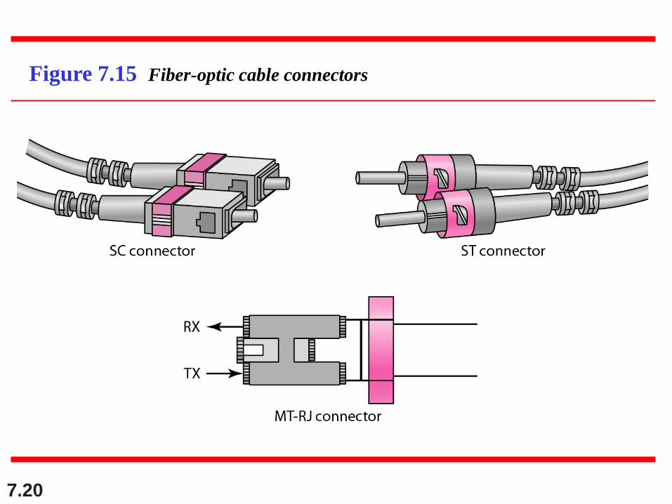
Figure 7.15 Fiber-optic cable connectors

7.21

Figure 7.16 Optical fiber performance

7.22

7-2 UNGUIDED MEDIA: WIRELESS

Unguided media transport electromagnetic waves

without using a physical conductor. This type of

communication is often referred to as wireless

communication.

Radio Waves

Microwaves

Infrared


7.23

Figure 7.17 Electromagnetic spectrum for wireless communication

7.24

Figure 7.18 Propagation methods

7.25

Table 7.4 Bands

7.26

Figure 7.19 Wireless transmission waves

7.27

Figure 7.20 Omnidirectional antenna

7.28

Radio waves are used for multicast

communications, such as radio and

television, and paging systems.

Note

7.29

Figure 7.21 Unidirectional antennas

7.30

Microwaves are used for unicast

communication such as cellular

telephones, satellite networks,

and wireless LANs.

Note

7.31

Infrared signals can be used for short-

range communication in a closed area

using line-of-sight propagation.

Note

9.1

Chapter 9

Using Telephone

and Cable Networks

for Data Transmission


9.2

9-1 TELEPHONE NETWORK

Telephone networks use circuit switching. The

telephone network had its beginnings in the late

1800s. The entire network, which is referred to as the

plain old telephone system (POTS), was originally an

analog system using analog signals to transmit voice.

Major Components

LATAs

Signaling

Services Provided by Telephone Networks


9.3

Figure 9.1 A telephone system

9.4

Intra-LATA services are provided by

local exchange carriers.

Since 1996, there are two

types of LECs: incumbent local

exchange carriers and competitive

local exchange carriers.

Note

9.5

Figure 9.2 Switching offices in a LATA

9.6

Figure 9.3 Point of presences (POPs)

9.7

The tasks of data transfer and signaling

are separated in modern telephone

networks: data transfer is done by one

network, signaling by another.

Note

9.8

Figure 9.4 Data transfer and signaling networks

9.9

Figure 9.5 Layers in SS7

9.10

9-2 DIAL-UP MODEMS

Traditional telephone lines can carry frequencies

between 300 and 3300 Hz, giving them a bandwidth of

3000 Hz. All this range is used for transmitting voice,

where a great deal of interference and distortion can

be accepted without loss of intelligibility.

Modem Standards


9.11

Figure 9.6 Telephone line bandwidth

9.12

Modem

stands for modulator/demodulator.

Note

9.13

Figure 9.7 Modulation/demodulation

9.14

Figure 9.8 The V.32 and V.32bis constellation and bandwidth

9.15

Figure 9.9 Uploading and downloading in 56K modems

9.16

9-3 DIGITAL SUBSCRIBER LINE

After traditional modems reached their peak data rate,

telephone companies developed another technology,

DSL, to provide higher-speed access to the Internet.

Digital subscriber line (DSL) technology is one of the

most promising for supporting high-speed digital

communication over the existing local loops.

ADSL

ADSL Lite

HDSL

SDSL

VDSL


9.17

ADSL is an asymmetric communication

technology designed for residential

users; it is not suitable for businesses.

Note

9.18

The existing local loops can handle

bandwidths up to 1.1 MHz.

Note

9.19

ADSL is an adaptive technology.

The system uses a data rate

based on the condition of

the local loop line.

Note

9.20

Figure 9.10 Discrete multitone technique

9.21

Figure 9.11 Bandwidth division in ADSL

9.22

Figure 9.12 ADSL modem

9.23

Figure 9.13 DSLAM

9.24

Table 9.2 Summary of DSL technologies

9.25

9-4 CABLE TV NETWORKS

The cable TV network started as a video service

provider, but it has moved to the business of Internet

access. In this section, we discuss cable TV networks

per se; in Section 9.5 we discuss how this network can

be used to provide high-speed access to the Internet.

Traditional Cable Networks

Hybrid Fiber-Coaxial (HFC) Network


9.26

Figure 9.14 Traditional cable TV network

9.27

Communication in the traditional cable

TV network is unidirectional.

Note

9.28

Figure 9.15 Hybrid fiber-coaxial (HFC) network

9.29

Communication in an HFC cable TV

network can be bidirectional.

Note

9.30

9-5 CABLE TV FOR DATA TRANSFER

Cable companies are now competing with telephone

companies for the residential customer who wants

high-speed data transfer. In this section, we briefly

discuss this technology.

Bandwidth

Sharing

CM and CMTS

Data Transmission Schemes: DOCSIS


9.31

Figure 9.16 Division of coaxial cable band by CATV

9.32

Downstream data are modulated using

the 64-QAM modulation technique.

Note

9.33

The theoretical downstream data rate

is 30 Mbps.

Note

9.34

Upstream data are modulated using the

QPSK modulation technique.

Note

9.35

The theoretical upstream data rate

is 12 Mbps.

Note

9.36

Figure 9.17 Cable modem (CM)

9.37

Figure 9.18 Cable modem transmission system (CMTS)

Chapter 3 Data and Signals - CSE IIT Kgp

Documents

Transcript of Chapter 3 Data and Signals - CSE IIT Kgp