Dynamic Indexability - cse hkust
96
1-1 Dynamic Indexability and Lower Bounds for Dynamic One-Dimensional Range Query Indexes Ke Yi HKUST
-
Upload
khangminh22 -
Category
Documents
-
view
0 -
download
0
Transcript of Dynamic Indexability - cse hkust

1-1
Dynamic Indexabilityand
Lower Bounds for DynamicOne-Dimensional Range Query Indexes
Ke Yi
HKUST
2-1
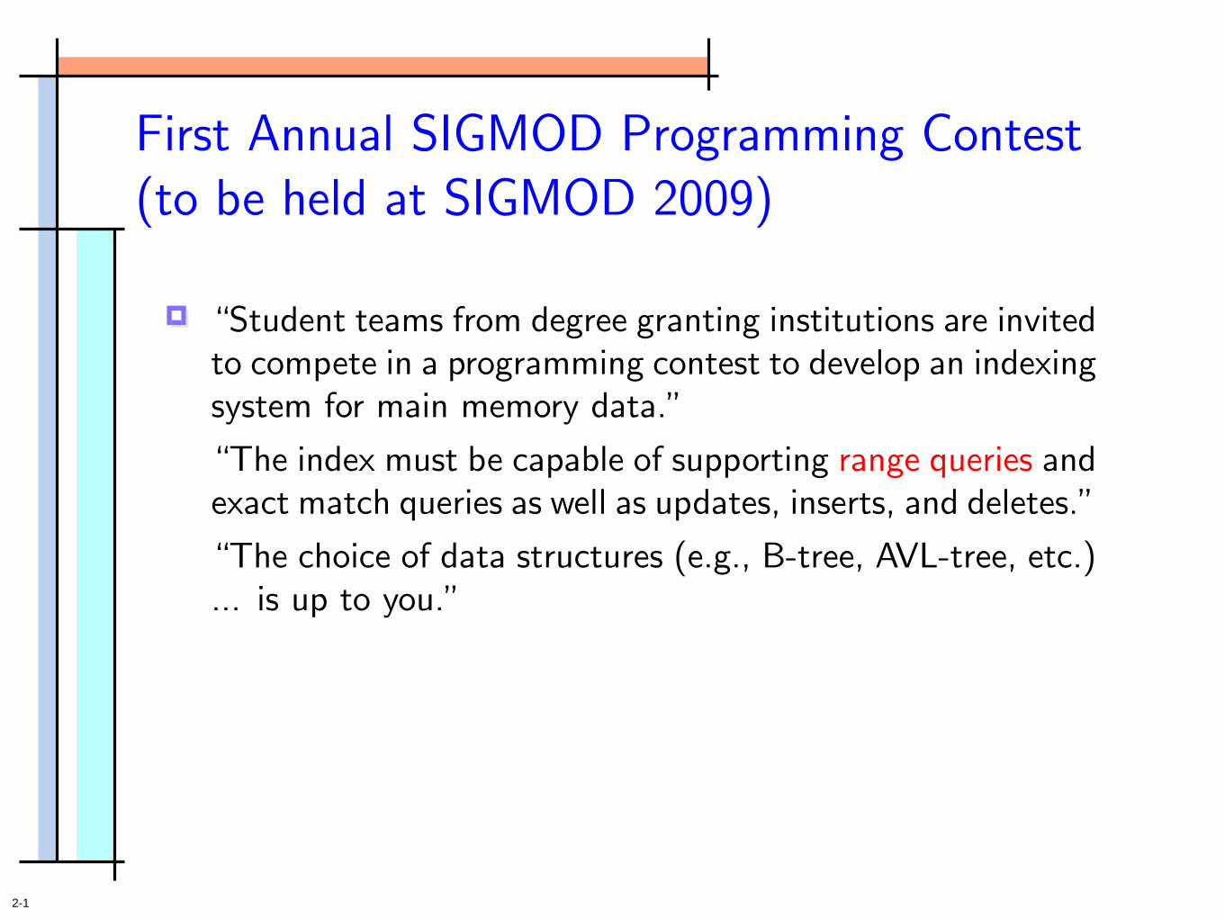
First Annual SIGMOD Programming Contest(to be held at SIGMOD 2009)
“Student teams from degree granting institutions are invitedto compete in a programming contest to develop an indexingsystem for main memory data.”
“The index must be capable of supporting range queries andexact match queries as well as updates, inserts, and deletes.”
“The choice of data structures (e.g., B-tree, AVL-tree, etc.)... is up to you.”

2-2
First Annual SIGMOD Programming Contest(to be held at SIGMOD 2009)
“Student teams from degree granting institutions are invitedto compete in a programming contest to develop an indexingsystem for main memory data.”
“The index must be capable of supporting range queries andexact match queries as well as updates, inserts, and deletes.”
“The choice of data structures (e.g., B-tree, AVL-tree, etc.)... is up to you.”
We think these problems are so basic that every DB gradstudent should know, but do we really have the answer?

3-1
Answer: Hash Table and B-tree!
Indeed, (external) hash tables and B-trees are both funda-mental index structures that are used in all database systems

3-2
Answer: Hash Table and B-tree!
Indeed, (external) hash tables and B-trees are both funda-mental index structures that are used in all database systems
Even for main memory data, we should still use external ver-sions that optimize cache misses

3-3
Answer: Hash Table and B-tree!
Indeed, (external) hash tables and B-trees are both funda-mental index structures that are used in all database systems
Even for main memory data, we should still use external ver-sions that optimize cache misses
External memory model (I/O model):
Each I/O reads/writes a block
Memory of size m
Disk partitioned into blocks of size b
Memory
Disk

4-1
The B-tree
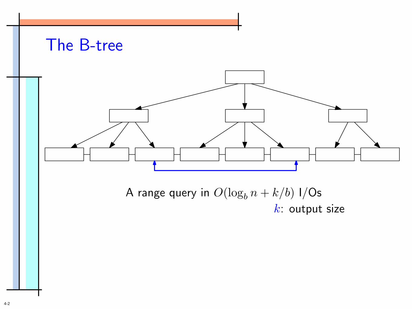
4-2
The B-tree
A range query in O(logb n+ k/b) I/Os
k: output size
4-3
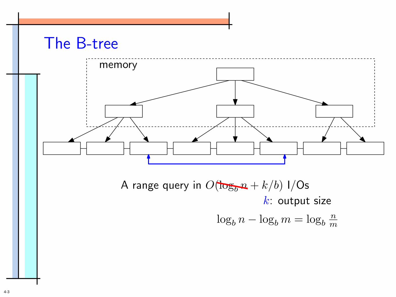
The B-tree
A range query in O(logb n+ k/b) I/Os
k: output size
memory
logb n− logbm = logbnm
4-4
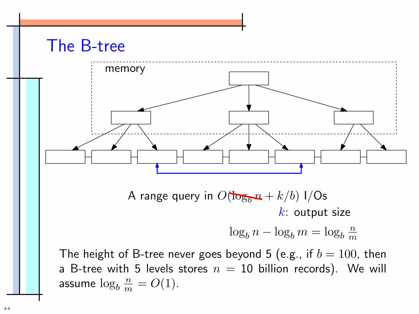
The B-tree
A range query in O(logb n+ k/b) I/Os
k: output size
memory
logb n− logbm = logbnm
The height of B-tree never goes beyond 5 (e.g., if b = 100, thena B-tree with 5 levels stores n = 10 billion records). We willassume logb
nm = O(1).

5-1
Now Let’s Go Dynamic
B-tree: Split blocks when necessary
Focus on insertions first: Both the B-tree and hash table do asearch first, then insert into the appropriate block
Hashing: Rebuild the hash table when too full; extensible hashing[Fagin, Nievergelt, Pippenger, Strong, 79]; linear hashing [Litwin,80]

5-2
Now Let’s Go Dynamic
B-tree: Split blocks when necessary
Focus on insertions first: Both the B-tree and hash table do asearch first, then insert into the appropriate block
These resizing operations only add O(1/b) I/Os amortized perinsertion; bottleneck is the first search + insert
Hashing: Rebuild the hash table when too full; extensible hashing[Fagin, Nievergelt, Pippenger, Strong, 79]; linear hashing [Litwin,80]

5-3
Now Let’s Go Dynamic
Cannot hope for lower than 1 I/O per insertion only if thechanges must be committed to disk right away (necessary?)
B-tree: Split blocks when necessary
Focus on insertions first: Both the B-tree and hash table do asearch first, then insert into the appropriate block
These resizing operations only add O(1/b) I/Os amortized perinsertion; bottleneck is the first search + insert
Hashing: Rebuild the hash table when too full; extensible hashing[Fagin, Nievergelt, Pippenger, Strong, 79]; linear hashing [Litwin,80]

5-4
Now Let’s Go Dynamic
Cannot hope for lower than 1 I/O per insertion only if thechanges must be committed to disk right away (necessary?)
B-tree: Split blocks when necessary
Otherwise we probably can lower the amortized insertion cost bybuffering, like numerous problems in external memory, e.g. stack,priority queue,... All of them support an insertion in O(1/b) I/Os— the best possible
Focus on insertions first: Both the B-tree and hash table do asearch first, then insert into the appropriate block
These resizing operations only add O(1/b) I/Os amortized perinsertion; bottleneck is the first search + insert
Hashing: Rebuild the hash table when too full; extensible hashing[Fagin, Nievergelt, Pippenger, Strong, 79]; linear hashing [Litwin,80]

6-1
Dynamic B-trees for Fast Insertions
LSM-tree [O’Neil, Cheng, Gawlick,O’Neil, 96]: Logarithmic method +B-tree
memory
`2m
`m
m

6-2
Dynamic B-trees for Fast Insertions
LSM-tree [O’Neil, Cheng, Gawlick,O’Neil, 96]: Logarithmic method +B-tree
memory
`2m
`m
m
Insertion: O( `b
log`nm
)
Query: O(log`nm
+ kb)

6-3
Dynamic B-trees for Fast Insertions
LSM-tree [O’Neil, Cheng, Gawlick,O’Neil, 96]: Logarithmic method +B-tree
memory
`2m
`m
m
Insertion: O( `b
log`nm
)
Query: O(log`nm
+ kb)
Stepped merge tree [Jagadish, Narayan, Seshadri, Sudar-shan, Kannegantil, 97]: variant of LSM-tree
Insertion: O( 1b
log`nm
)
Query: O(` log`nm
+ kb)

6-4
Dynamic B-trees for Fast Insertions
LSM-tree [O’Neil, Cheng, Gawlick,O’Neil, 96]: Logarithmic method +B-tree
memory
`2m
`m
m
Insertion: O( `b
log`nm
)
Query: O(log`nm
+ kb)
Stepped merge tree [Jagadish, Narayan, Seshadri, Sudar-shan, Kannegantil, 97]: variant of LSM-tree
Insertion: O( 1b
log`nm
)
Query: O(` log`nm
+ kb)
Usually ` is set to be a constant, then they both haveO( 1
b log nm ) insertion and O(log n
m + kb ) query

7-1
More Dynamic B-trees
Yet another B-tree (Y-tree) [Jermaine, Datta, Omiecinski, 99]
Buffer tree [Arge, 95]
7-2
More Dynamic B-trees
Yet another B-tree (Y-tree) [Jermaine, Datta, Omiecinski, 99]
Insertion: O( 1b
log nm
), pretty fast since b log nm
typically, butnot that fast; if O( 1
b) insertion required, query becomes O(bε + k
b)
Buffer tree [Arge, 95]
Query: O(log nm
+ kb), much worse than the static B-tree’s O(1+ k
b);
if O(1 + kb) query required, insertion cost becomes O( b
ε
b)
7-3
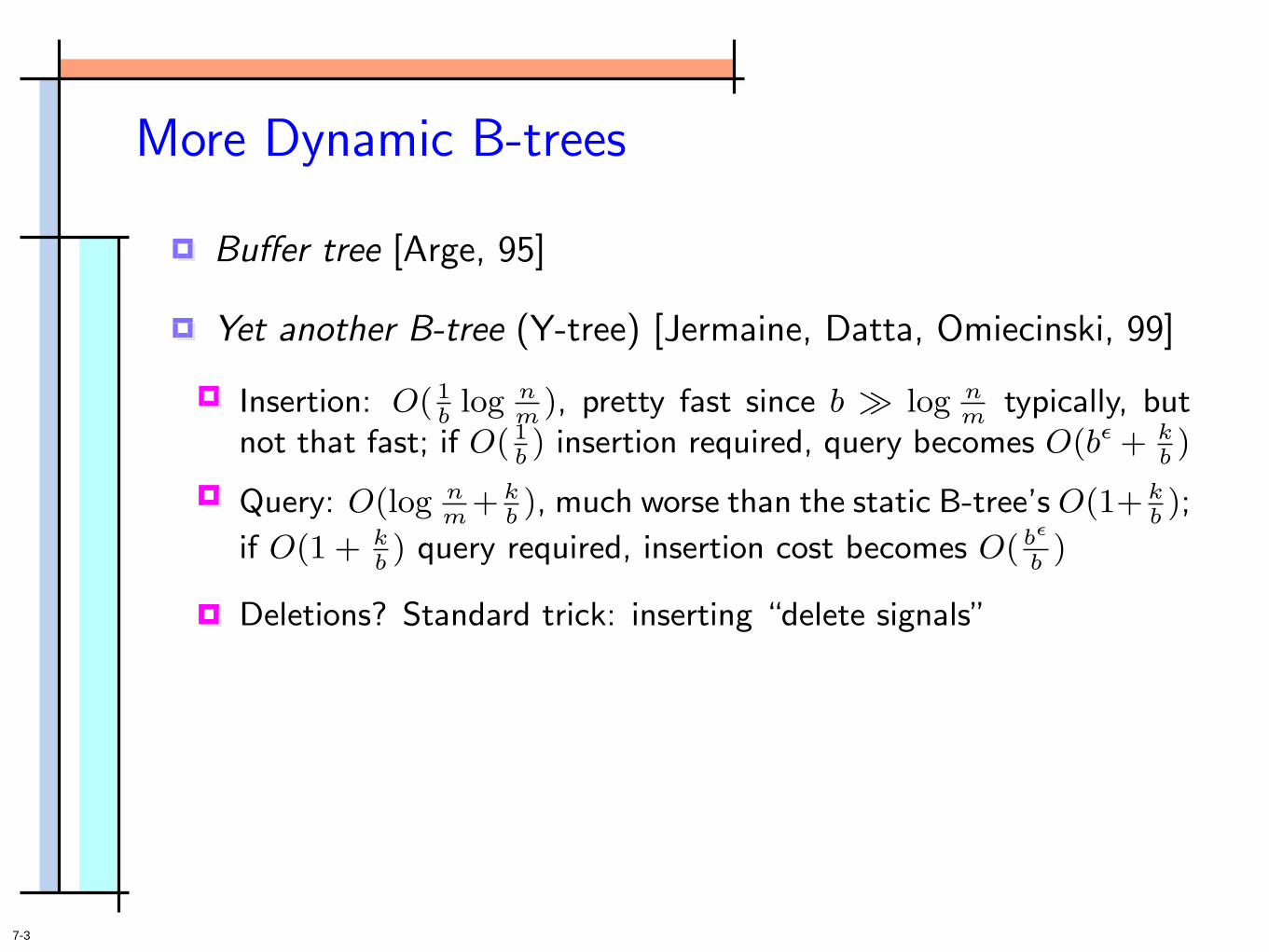
More Dynamic B-trees
Yet another B-tree (Y-tree) [Jermaine, Datta, Omiecinski, 99]
Insertion: O( 1b
log nm
), pretty fast since b log nm
typically, butnot that fast; if O( 1
b) insertion required, query becomes O(bε + k
b)
Buffer tree [Arge, 95]
Query: O(log nm
+ kb), much worse than the static B-tree’s O(1+ k
b);
if O(1 + kb) query required, insertion cost becomes O( b
ε
b)
Deletions? Standard trick: inserting “delete signals”
7-4
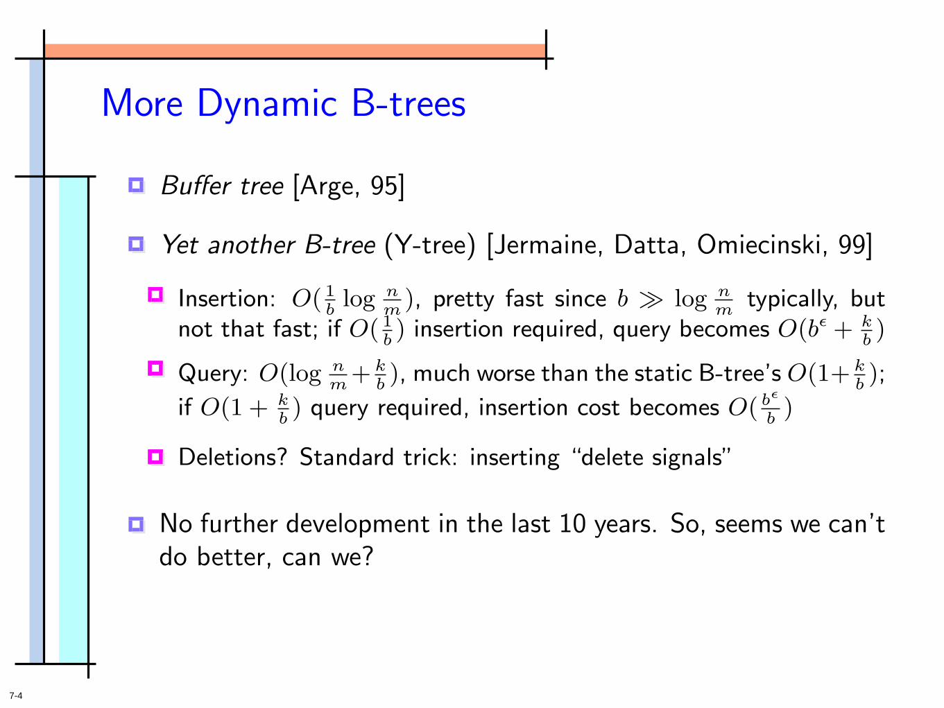
More Dynamic B-trees
Yet another B-tree (Y-tree) [Jermaine, Datta, Omiecinski, 99]
Insertion: O( 1b
log nm
), pretty fast since b log nm
typically, butnot that fast; if O( 1
b) insertion required, query becomes O(bε + k
b)
No further development in the last 10 years. So, seems we can’tdo better, can we?
Buffer tree [Arge, 95]
Query: O(log nm
+ kb), much worse than the static B-tree’s O(1+ k
b);
if O(1 + kb) query required, insertion cost becomes O( b
ε
b)
Deletions? Standard trick: inserting “delete signals”

8-1
Main Result
For any dynamic range query index with a query cost of q+O(k/b)and an amortized insertion cost of u/b, the following tradeoff holds
q · log(u/q) = Ω(log b), for q < α ln b, α is any constant;u · log q = Ω(log b), for all q.

8-2
Main Result
For any dynamic range query index with a query cost of q+O(k/b)and an amortized insertion cost of u/b, the following tradeoff holds
q · log(u/q) = Ω(log b), for q < α ln b, α is any constant;u · log q = Ω(log b), for all q.
Current upper bounds:q u
log nm log n
m
1 ( nm )ε
( nm )ε 1

8-3
Main Result
For any dynamic range query index with a query cost of q+O(k/b)and an amortized insertion cost of u/b, the following tradeoff holds
q · log(u/q) = Ω(log b), for q < α ln b, α is any constant;u · log q = Ω(log b), for all q.
Current upper bounds:q u
log nm log n
m
1 ( nm )ε
( nm )ε 1
Assuming logbnm
= O(1), all the bounds are tight!

8-4
Main Result
For any dynamic range query index with a query cost of q+O(k/b)and an amortized insertion cost of u/b, the following tradeoff holds
q · log(u/q) = Ω(log b), for q < α ln b, α is any constant;u · log q = Ω(log b), for all q.
Current upper bounds:q u
log nm log n
m
1 ( nm )ε
( nm )ε 1
Assuming logbnm
= O(1), all the bounds are tight!
The technique of [Brodal, Fagerberg, 03] for the predecessor prob-lem can be used to derive a tradeoff of
q · log(u log2 nm ) = Ω(log n
m ).
9-1
Lower Bound Model: Dynamic Indexability
Indexability: [Hellerstein, Koutsoupias, Papadimitriou, 97]

9-2
Lower Bound Model: Dynamic Indexability
Indexability: [Hellerstein, Koutsoupias, Papadimitriou, 97]
4 7 9 1 2 4 3 5 8 2 6 7 1 8 9 4 5
Objects are stored in disk blocks of size up to b, possibly withredundancy.Redundancy r = (total # blocks)/dn/be
9-3
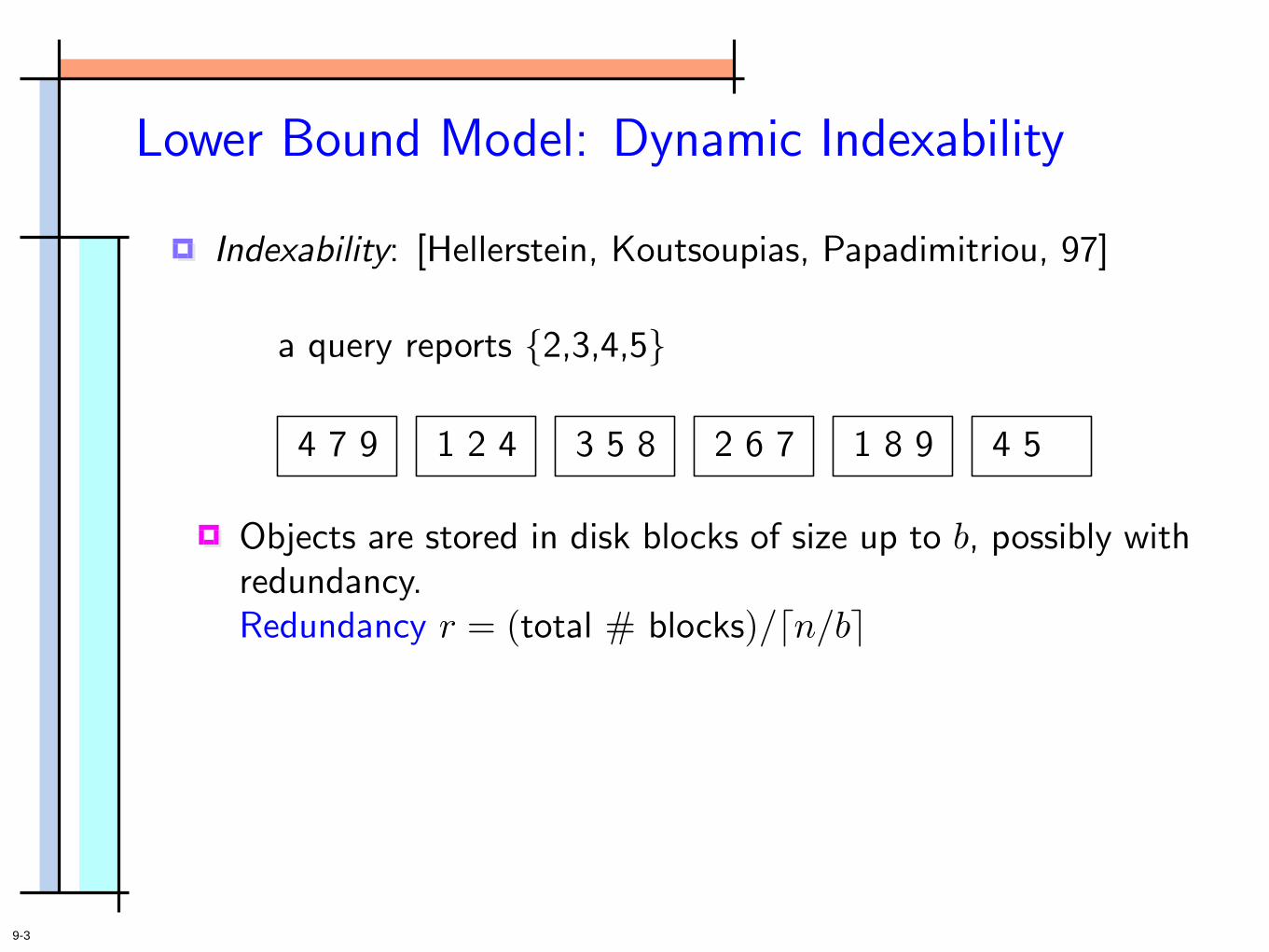
Lower Bound Model: Dynamic Indexability
Indexability: [Hellerstein, Koutsoupias, Papadimitriou, 97]
4 7 9 1 2 4 3 5 8 2 6 7 1 8 9 4 5
Objects are stored in disk blocks of size up to b, possibly withredundancy.Redundancy r = (total # blocks)/dn/be
a query reports 2,3,4,5

9-4
Lower Bound Model: Dynamic Indexability
Indexability: [Hellerstein, Koutsoupias, Papadimitriou, 97]
4 7 9 1 2 4 3 5 8 2 6 7 1 8 9 4 5
Objects are stored in disk blocks of size up to b, possibly withredundancy.Redundancy r = (total # blocks)/dn/be
a query reports 2,3,4,5
The query cost is the minimum number of blocks that cancover all the required results (search time ignored!).Access overhead A = (worst-case) query cost /dk/be
cost = 2

9-5
Lower Bound Model: Dynamic Indexability
Indexability: [Hellerstein, Koutsoupias, Papadimitriou, 97]
4 7 9 1 2 4 3 5 8 2 6 7 1 8 9 4 5
Objects are stored in disk blocks of size up to b, possibly withredundancy.Redundancy r = (total # blocks)/dn/be
a query reports 2,3,4,5
The query cost is the minimum number of blocks that cancover all the required results (search time ignored!).Access overhead A = (worst-case) query cost /dk/be
cost = 2
Similar in spirit to popular lower bound models: cell probemodel, semigroup model

10-1
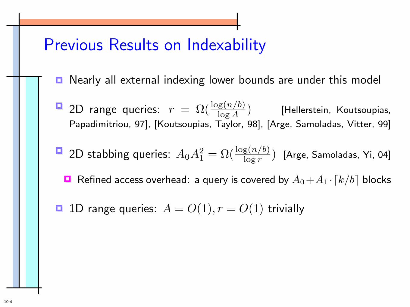
Previous Results on Indexability
Nearly all external indexing lower bounds are under this model

10-2
Previous Results on Indexability
2D range queries: r = Ω( log(n/b)logA ) [Hellerstein, Koutsoupias,
Papadimitriou, 97], [Koutsoupias, Taylor, 98], [Arge, Samoladas, Vitter, 99]
Nearly all external indexing lower bounds are under this model

10-3
Previous Results on Indexability
2D range queries: r = Ω( log(n/b)logA ) [Hellerstein, Koutsoupias,
Papadimitriou, 97], [Koutsoupias, Taylor, 98], [Arge, Samoladas, Vitter, 99]
2D stabbing queries: A0A21 = Ω( log(n/b)
log r ) [Arge, Samoladas, Yi, 04]
Refined access overhead: a query is covered by A0+A1 ·dk/be blocks
Nearly all external indexing lower bounds are under this model
10-4
Previous Results on Indexability
2D range queries: r = Ω( log(n/b)logA ) [Hellerstein, Koutsoupias,
Papadimitriou, 97], [Koutsoupias, Taylor, 98], [Arge, Samoladas, Vitter, 99]
2D stabbing queries: A0A21 = Ω( log(n/b)
log r ) [Arge, Samoladas, Yi, 04]
Refined access overhead: a query is covered by A0+A1 ·dk/be blocks
1D range queries: A = O(1), r = O(1) trivially
Nearly all external indexing lower bounds are under this model

10-5
Previous Results on Indexability
2D range queries: r = Ω( log(n/b)logA ) [Hellerstein, Koutsoupias,
Papadimitriou, 97], [Koutsoupias, Taylor, 98], [Arge, Samoladas, Vitter, 99]
2D stabbing queries: A0A21 = Ω( log(n/b)
log r ) [Arge, Samoladas, Yi, 04]
Refined access overhead: a query is covered by A0+A1 ·dk/be blocks
1D range queries: A = O(1), r = O(1) trivially
Adding dynamization makes it much more interesting!
Nearly all external indexing lower bounds are under this model

11-1
Dynamic Indexability
Still consider only insertions

11-2
Dynamic Indexability
Still consider only insertions
4 5time t:
memory of size m
4 7 9 ← snapshot1 2 7
blocks of size b = 3

11-3
Dynamic Indexability
Still consider only insertions
4 5time t:
memory of size m
4 7 9 ← snapshot1 2 7
blocks of size b = 3
4 5time t+ 1: 4 7 91 2 6 7 6 inserted

11-4
Dynamic Indexability
Still consider only insertions
4 5time t:
memory of size m
4 7 9 ← snapshot1 2 7
1 2 6 7
8 inserted
blocks of size b = 3
4 5time t+ 1: 4 7 91 2 6 7 6 inserted
1 2 5time t+ 2: 4 7 9 6 8

11-5
Dynamic Indexability
Still consider only insertions
4 5time t:
memory of size m
4 7 9 ← snapshot1 2 7
1 2 6 7
8 inserted
blocks of size b = 3
4 5time t+ 1: 4 7 91 2 6 7 6 inserted
1 2 5time t+ 2: 4 7 9 6 8
transition cost = 2

11-6
Dynamic Indexability
Still consider only insertions
4 5time t:
memory of size m
4 7 9 ← snapshot1 2 7
1 2 6 7
8 inserted
blocks of size b = 3
4 5time t+ 1: 4 7 91 2 6 7 6 inserted
1 2 5time t+ 2: 4 7 9 6 8
transition cost = 2
Redundancy (access overhead) is the worst redundancy (accessoverhead) of all snapshots

11-7
Dynamic Indexability
Still consider only insertions
4 5time t:
memory of size m
4 7 9 ← snapshot1 2 7
1 2 6 7
8 inserted
blocks of size b = 3
4 5time t+ 1: 4 7 91 2 6 7 6 inserted
1 2 5time t+ 2: 4 7 9 6 8
transition cost = 2
Redundancy (access overhead) is the worst redundancy (accessoverhead) of all snapshots
Update cost: u = the average transition cost per b insertions

12-1
Main Result Obtained in Dynamic Indexability
Theorem: For any dynamic 1D range query index with accessoverhead A and update cost u, the following tradeoff holds, pro-vided n ≥ 2mb2:
A · log(u/A) = Ω(log b), for A < α ln b, α is any constant;u · logA = Ω(log b), for all A.

12-2
Main Result Obtained in Dynamic Indexability
Theorem: For any dynamic 1D range query index with accessoverhead A and update cost u, the following tradeoff holds, pro-vided n ≥ 2mb2:
A · log(u/A) = Ω(log b), for A < α ln b, α is any constant;u · logA = Ω(log b), for all A.
Because a query cost O(q + dk/be) implies O(q · dk/be)

12-3
Main Result Obtained in Dynamic Indexability
Theorem: For any dynamic 1D range query index with accessoverhead A and update cost u, the following tradeoff holds, pro-vided n ≥ 2mb2:
A · log(u/A) = Ω(log b), for A < α ln b, α is any constant;u · logA = Ω(log b), for all A.
Because a query cost O(q + dk/be) implies O(q · dk/be)
The lower bound doesn’t depend on the redundancy r!

13-1
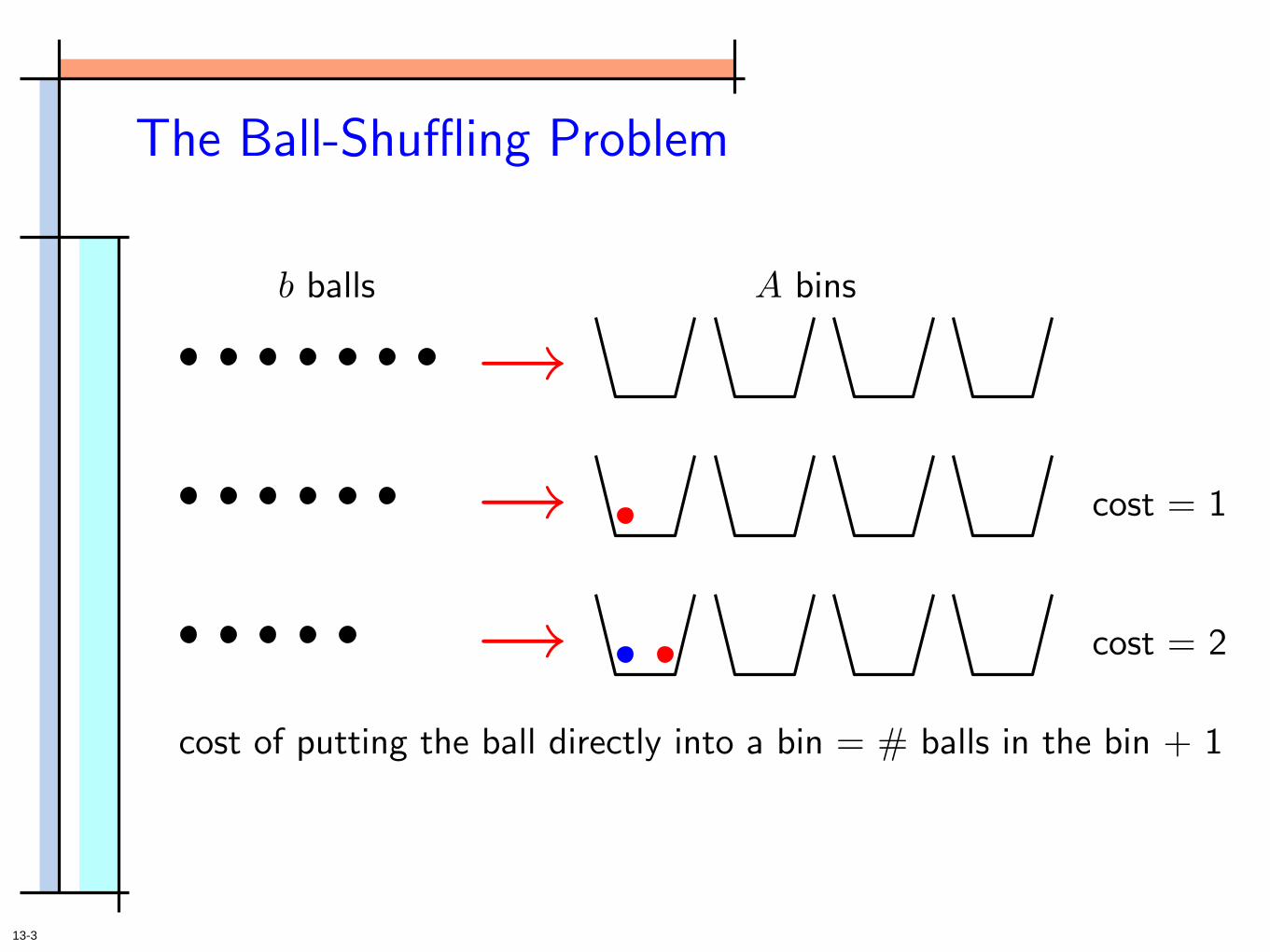
The Ball-Shuffling Problem
→b balls A bins

13-2
The Ball-Shuffling Problem
→b balls A bins
→ cost = 1
13-3
The Ball-Shuffling Problem
→b balls A bins
→ cost = 1
→ cost = 2
cost of putting the ball directly into a bin = # balls in the bin + 1

14-1
The Ball-Shuffling Problem
→b balls A bins

14-2
The Ball-Shuffling Problem
→b balls A bins
→ cost = 5Shuffle:

14-3
The Ball-Shuffling Problem
→b balls A bins
→ cost = 5
Cost of shuffling = # balls in the involved bins
Shuffle:

14-4
The Ball-Shuffling Problem
→b balls A bins
→ cost = 5
Cost of shuffling = # balls in the involved bins
Shuffle:
Putting a ball directly into a bin is a special shuffle

14-5
The Ball-Shuffling Problem
→b balls A bins
→ cost = 5
Cost of shuffling = # balls in the involved bins
Shuffle:
Putting a ball directly into a bin is a special shuffle
Goal: Accommodating all b balls using A bins with minimum cost

15-1
Ball-Shuffling Lower Bounds
Theorem: The cost of any solution for the ball-shuffling problemis at least
Ω(A · b1+Ω(1/A)), for A < α ln b where α is any constant;Ω(b logA b), for any A.
A
cost lower bound

15-2
Ball-Shuffling Lower Bounds
Theorem: The cost of any solution for the ball-shuffling problemis at least
Ω(A · b1+Ω(1/A)), for A < α ln b where α is any constant;Ω(b logA b), for any A.
A
cost lower bound
1
b2

15-3
Ball-Shuffling Lower Bounds
Theorem: The cost of any solution for the ball-shuffling problemis at least
Ω(A · b1+Ω(1/A)), for A < α ln b where α is any constant;Ω(b logA b), for any A.
A
cost lower bound
1
b2
b4/3
2

15-4
Ball-Shuffling Lower Bounds
Theorem: The cost of any solution for the ball-shuffling problemis at least
Ω(A · b1+Ω(1/A)), for A < α ln b where α is any constant;Ω(b logA b), for any A.
A
cost lower bound
1
b2
b4/3
2 log b
b log b

15-5
Ball-Shuffling Lower Bounds
Theorem: The cost of any solution for the ball-shuffling problemis at least
Ω(A · b1+Ω(1/A)), for A < α ln b where α is any constant;Ω(b logA b), for any A.
A
cost lower bound
1
b2
b4/3
2 log b
b log b
bε
b

15-6
Ball-Shuffling Lower Bounds
Theorem: The cost of any solution for the ball-shuffling problemis at least
Ω(A · b1+Ω(1/A)), for A < α ln b where α is any constant;Ω(b logA b), for any A.
A
cost lower bound
1
b2
b4/3
2 log b
b log b
bε
b
Tight (ignoring constants in big-Omega)for A = O(log b) and A = Ω(log1+ε b)
16-1
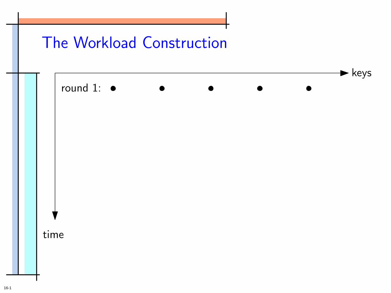
The Workload Construction
round 1:
keys
time

16-2
The Workload Construction
round 1:
round 2:
keys
time

16-3
The Workload Construction
round 1:
round 2:
keys
time
round 3:
· · ·
round b:

16-4
The Workload Construction
round 1:
round 2:
keys
time
round 3:
· · ·
round b:
Queries that we require the index to cover with A blocks# queries ≥ 2mb

16-5
The Workload Construction
round 1:
round 2:
keys
time
round 3:
· · ·
round b:
Queries that we require the index to cover with A blocks# queries ≥ 2mb
snapshot
snapshot
snapshot
snapshot
Snapshots of the dynamic index considered

17-1
The Workload Construction
round 1:
keys
time
round 2:
round 3:· · ·
round b:
There exists a query such that
• The ≤ b objects of the query reside in ≤ A blocksin all snapshots
• All of its objects are on disk in all b snapshots (wehave ≥ mb queries)
• The index moves its objects ub times in total
18-1
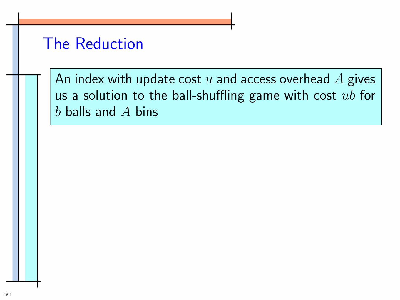
The Reduction
An index with update cost u and access overhead A givesus a solution to the ball-shuffling game with cost ub forb balls and A bins

18-2
The Reduction
An index with update cost u and access overhead A givesus a solution to the ball-shuffling game with cost ub forb balls and A bins
Lower bound on the ball-shuffling problem:
Theorem: The cost of any solution for the ball-shuffling problemis at least
Ω(A · b1+Ω(1/A)), for A < α ln b where α is any constant;Ω(b logA b), for any A.

18-3
The Reduction
An index with update cost u and access overhead A givesus a solution to the ball-shuffling game with cost ub forb balls and A bins
Lower bound on the ball-shuffling problem:
Theorem: The cost of any solution for the ball-shuffling problemis at least
Ω(A · b1+Ω(1/A)), for A < α ln b where α is any constant;Ω(b logA b), for any A.
A · log(u/A) = Ω(log b), for A < α ln b, α is any constant;u · logA = Ω(log b), for all A.
⇒

19-1
Ball-Shuffling Lower Bound Proof
Ω(A · b1+Ω(1/A)), for A < α ln b where α is any constant;Ω(b logA b), for any A.

19-2
Ball-Shuffling Lower Bound Proof
Ω(A · b1+Ω(1/A)), for A < α ln b where α is any constant;Ω(b logA b), for any A.
Will show: Any algorithm that handles the balls with an averagecost of u using A bins cannot accommodate (2A)2u balls ormore. ⇒b < (2A)2u, or u > log b
2 log(2A) , so the total cost of the algorithm
is ub = Ω(b logA b).

19-3
Ball-Shuffling Lower Bound Proof
Ω(A · b1+Ω(1/A)), for A < α ln b where α is any constant;Ω(b logA b), for any A.
Will show: Any algorithm that handles the balls with an averagecost of u using A bins cannot accommodate (2A)2u balls ormore. ⇒b < (2A)2u, or u > log b
2 log(2A) , so the total cost of the algorithm
is ub = Ω(b logA b).
Prove by induction on u
u = 1: Can handle at most A balls.

19-4
Ball-Shuffling Lower Bound Proof
Ω(A · b1+Ω(1/A)), for A < α ln b where α is any constant;Ω(b logA b), for any A.
Will show: Any algorithm that handles the balls with an averagecost of u using A bins cannot accommodate (2A)2u balls ormore. ⇒b < (2A)2u, or u > log b
2 log(2A) , so the total cost of the algorithm
is ub = Ω(b logA b).
Prove by induction on u
u = 1: Can handle at most A balls.
u→ u+ 12 ?

20-1
Ball-Shuffling Lower Bound Proof (2)
Need tol show: Any algorithm that handles the balls with an av-erage cost of u+ 1
2 using A bins cannot accommodate (2A)2u+1
balls or more. ⇔
To handle (2A)2u+1 balls, any algorithm has to pay an averagecost of more than u+ 1
2 per ball, or(u+
12
)(2A)2u+1 = (2Au+A)(2A)2u
in total.

20-2
Ball-Shuffling Lower Bound Proof (2)
Need tol show: Any algorithm that handles the balls with an av-erage cost of u+ 1
2 using A bins cannot accommodate (2A)2u+1
balls or more. ⇔
To handle (2A)2u+1 balls, any algorithm has to pay an averagecost of more than u+ 1
2 per ball, or(u+
12
)(2A)2u+1 = (2Au+A)(2A)2u
in total.
Divide all balls into 2A batches of (2A)2u each.

20-3
Ball-Shuffling Lower Bound Proof (2)
Need tol show: Any algorithm that handles the balls with an av-erage cost of u+ 1
2 using A bins cannot accommodate (2A)2u+1
balls or more. ⇔
To handle (2A)2u+1 balls, any algorithm has to pay an averagecost of more than u+ 1
2 per ball, or(u+
12
)(2A)2u+1 = (2Au+A)(2A)2u
in total.
Divide all balls into 2A batches of (2A)2u each.
Accommodating each batch by itself costs u(2A)2u

21-1
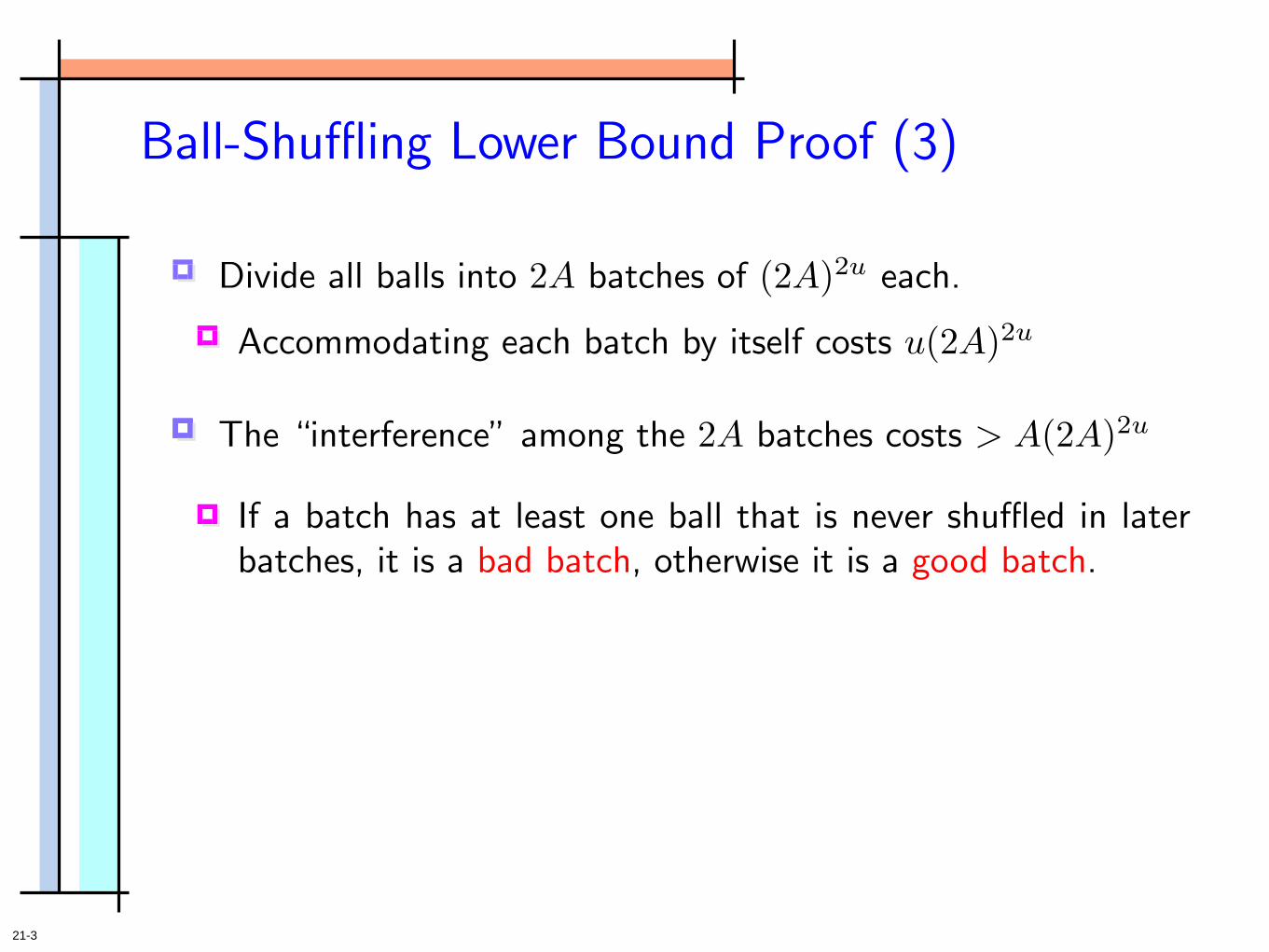
Divide all balls into 2A batches of (2A)2u each.
Accommodating each batch by itself costs u(2A)2u
Ball-Shuffling Lower Bound Proof (3)

21-2
Divide all balls into 2A batches of (2A)2u each.
Accommodating each batch by itself costs u(2A)2u
Ball-Shuffling Lower Bound Proof (3)
The “interference” among the 2A batches costs > A(2A)2u
21-3
Divide all balls into 2A batches of (2A)2u each.
Accommodating each batch by itself costs u(2A)2u
Ball-Shuffling Lower Bound Proof (3)
If a batch has at least one ball that is never shuffled in laterbatches, it is a bad batch, otherwise it is a good batch.
The “interference” among the 2A batches costs > A(2A)2u

21-4
Divide all balls into 2A batches of (2A)2u each.
Accommodating each batch by itself costs u(2A)2u
Ball-Shuffling Lower Bound Proof (3)
If a batch has at least one ball that is never shuffled in laterbatches, it is a bad batch, otherwise it is a good batch.
The “interference” among the 2A batches costs > A(2A)2u
There are at most A bad batches

21-5
Divide all balls into 2A batches of (2A)2u each.
Accommodating each batch by itself costs u(2A)2u
Ball-Shuffling Lower Bound Proof (3)
If a batch has at least one ball that is never shuffled in laterbatches, it is a bad batch, otherwise it is a good batch.
The “interference” among the 2A batches costs > A(2A)2u
There are at most A bad batches
There are at least A good batches

21-6
Divide all balls into 2A batches of (2A)2u each.
Accommodating each batch by itself costs u(2A)2u
Ball-Shuffling Lower Bound Proof (3)
If a batch has at least one ball that is never shuffled in laterbatches, it is a bad batch, otherwise it is a good batch.
The “interference” among the 2A batches costs > A(2A)2u
There are at most A bad batches
There are at least A good batches
Each good batch contributes at least (2A)2u to the “interfer-ence” cost
22-1
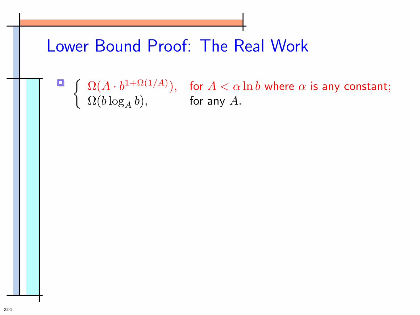
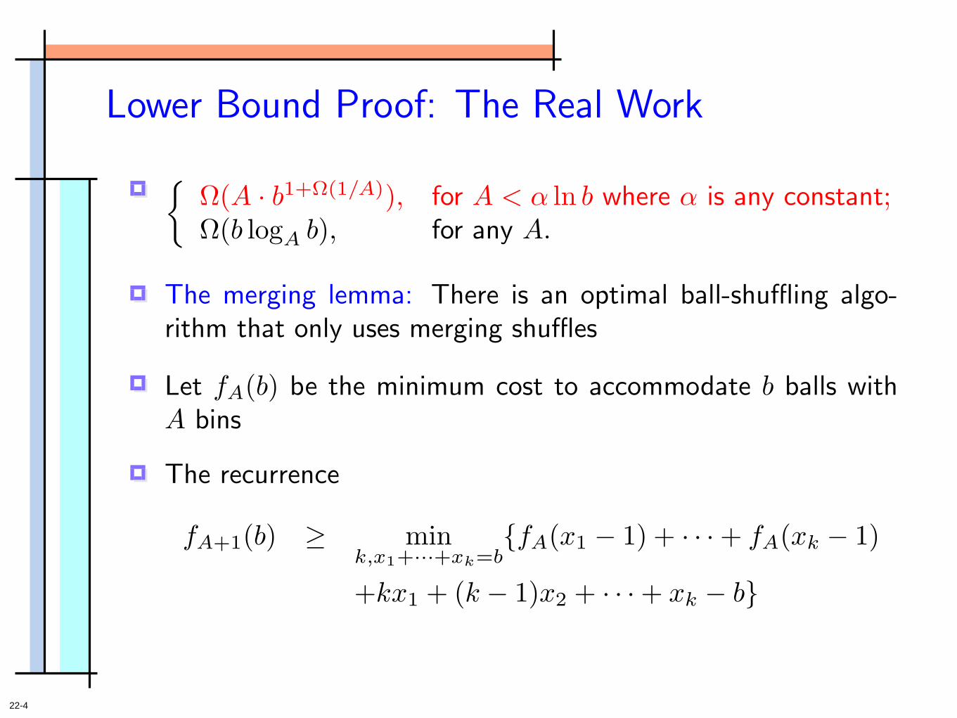
Lower Bound Proof: The Real Work
Ω(A · b1+Ω(1/A)), for A < α ln b where α is any constant;Ω(b logA b), for any A.

22-2
Lower Bound Proof: The Real Work
Ω(A · b1+Ω(1/A)), for A < α ln b where α is any constant;Ω(b logA b), for any A.
The merging lemma: There is an optimal ball-shuffling algo-rithm that only uses merging shuffles

22-3
Lower Bound Proof: The Real Work
Ω(A · b1+Ω(1/A)), for A < α ln b where α is any constant;Ω(b logA b), for any A.
Let fA(b) be the minimum cost to accommodate b balls withA bins
The merging lemma: There is an optimal ball-shuffling algo-rithm that only uses merging shuffles
22-4
Lower Bound Proof: The Real Work
Ω(A · b1+Ω(1/A)), for A < α ln b where α is any constant;Ω(b logA b), for any A.
Let fA(b) be the minimum cost to accommodate b balls withA bins
The recurrence
fA+1(b) ≥ mink,x1+···+xk=b
fA(x1 − 1) + · · ·+ fA(xk − 1)
+kx1 + (k − 1)x2 + · · ·+ xk − b
The merging lemma: There is an optimal ball-shuffling algo-rithm that only uses merging shuffles

23-1
Open Problems and Conjectures
1D range reporting
Current lower bound: query Ω(log b), update Ω( 1b log b). Im-
prove to (log nm , 1
b log nm )?

23-2
Open Problems and Conjectures
1D range reporting
Current lower bound: query Ω(log b), update Ω( 1b log b). Im-
prove to (log nm , 1
b log nm )?
Closely related problems: range sum (partial sum), predecessorsearch

24-1
The Grant Conjecture
range reporting
range sum
predecessor
Internal memory (RAM) External memory
O : (log n, log n)binary treeΩ : (log n, log n)[Patrascu, Demaine, 06]
w: word size b: block size (in words)

24-2
The Grant Conjecture
range reporting
range sum
predecessor
Internal memory (RAM) External memory
O : (log n, log n)binary treeΩ : (log n, log n)[Patrascu, Demaine, 06]
O : query = update =
min
log logn logwlog logw
,√
lognlog logn
Ω : . . .[Beame, Fich, 02]
w: word size b: block size (in words)

24-3
The Grant Conjecture
range reporting
range sum
predecessor
Internal memory (RAM) External memory
O : (log n, log n)binary treeΩ : (log n, log n)[Patrascu, Demaine, 06]
O : query = update =
min
log logn logwlog logw
,√
lognlog logn
Ω : . . .[Beame, Fich, 02]
O : (log log w, log w)O : (log log n, log n/ log log n)[Mortensen, Pagh, Patrascu, 05]Ω : open
w: word size b: block size (in words)
24-4
The Grant Conjecture
range reporting
range sum
predecessor
Internal memory (RAM) External memory
O : (log n, log n)binary treeΩ : (log n, log n)[Patrascu, Demaine, 06]
O : query = update =
min
log logn logwlog logw
,√
lognlog logn
Ω : . . .[Beame, Fich, 02]
O : (log log w, log w)O : (log log n, log n/ log log n)[Mortensen, Pagh, Patrascu, 05]Ω : open
w: word size b: block size (in words)
O : (log`nm
, `b
log`nm
)
B-tree + logarithmicmethod

24-5
The Grant Conjecture
range reporting
range sum
predecessor
Internal memory (RAM) External memory
O : (log n, log n)binary treeΩ : (log n, log n)[Patrascu, Demaine, 06]
O : query = update =
min
log logn logwlog logw
,√
lognlog logn
Ω : . . .[Beame, Fich, 02]
O : (log log w, log w)O : (log log n, log n/ log log n)[Mortensen, Pagh, Patrascu, 05]Ω : open
w: word size b: block size (in words)
O : (log`nm
, `b
log`nm
)
B-tree + logarithmicmethod
Optimal for all three?

24-6
The Grant Conjecture
range reporting
range sum
predecessor
Internal memory (RAM) External memory
O : (log n, log n)binary treeΩ : (log n, log n)[Patrascu, Demaine, 06]
O : query = update =
min
log logn logwlog logw
,√
lognlog logn
Ω : . . .[Beame, Fich, 02]
O : (log log w, log w)O : (log log n, log n/ log log n)[Mortensen, Pagh, Patrascu, 05]Ω : open
w: word size b: block size (in words)
O : (log`nm
, `b
log`nm
)
B-tree + logarithmicmethod
Optimal for all three?
How large does b needto be for B-tree to beoptimal?

24-7
The Grant Conjecture
range reporting
range sum
predecessor
Internal memory (RAM) External memory
O : (log n, log n)binary treeΩ : (log n, log n)[Patrascu, Demaine, 06]
O : query = update =
min
log logn logwlog logw
,√
lognlog logn
Ω : . . .[Beame, Fich, 02]
O : (log log w, log w)O : (log log n, log n/ log log n)[Mortensen, Pagh, Patrascu, 05]Ω : open
w: word size b: block size (in words)
O : (log`nm
, `b
log`nm
)
B-tree + logarithmicmethod
Optimal for all three?
How large does b needto be for B-tree to beoptimal?
We now know this is truefor range reporting forb = ( n
m)Ω(1); false for
b = o(log log n)

25-1
The End
T HANK YOU
Q and A