Linear Algebra - Department of Mathematics, HKUST
287
Linear Algebra Min Yan November 11, 2021
-
Upload
khangminh22 -
Category
Documents
-
view
0 -
download
0
Transcript of Linear Algebra - Department of Mathematics, HKUST

Linear Algebra
Min Yan
November 11, 2021

2

Contents
1 Vector Space 71.1 Definition . . . . . . . . . . . . . . . . . . . . . . . . . . . . . . . . . 7
1.1.1 Axioms of Vector Space . . . . . . . . . . . . . . . . . . . . . 71.1.2 Proof by Axiom . . . . . . . . . . . . . . . . . . . . . . . . . . 11
1.2 Linear Combination . . . . . . . . . . . . . . . . . . . . . . . . . . . . 121.2.1 Linear Combination Expression . . . . . . . . . . . . . . . . . 121.2.2 Row Operation . . . . . . . . . . . . . . . . . . . . . . . . . . 151.2.3 Row Echelon Form . . . . . . . . . . . . . . . . . . . . . . . . 171.2.4 Reduced Row Echelon Form . . . . . . . . . . . . . . . . . . . 19
1.3 Basis . . . . . . . . . . . . . . . . . . . . . . . . . . . . . . . . . . . . 211.3.1 Basis and Coordinate . . . . . . . . . . . . . . . . . . . . . . . 211.3.2 Spanning Set . . . . . . . . . . . . . . . . . . . . . . . . . . . 241.3.3 Linear Independence . . . . . . . . . . . . . . . . . . . . . . . 271.3.4 Minimal Spanning Set . . . . . . . . . . . . . . . . . . . . . . 311.3.5 Maximal Independent Set . . . . . . . . . . . . . . . . . . . . 331.3.6 Dimension . . . . . . . . . . . . . . . . . . . . . . . . . . . . . 351.3.7 Calculation of Coordinate . . . . . . . . . . . . . . . . . . . . 38
2 Linear Transformation 412.1 Linear Transformation and Matrix . . . . . . . . . . . . . . . . . . . 41
2.1.1 Linear Transformation of Linear Combination . . . . . . . . . 432.1.2 Linear Transformation between Euclidean Spaces . . . . . . . 452.1.3 Operation of Linear Transformation . . . . . . . . . . . . . . . 492.1.4 Matrix Operation . . . . . . . . . . . . . . . . . . . . . . . . . 512.1.5 Elementary Matrix and LU-Decomposition . . . . . . . . . . . 56
2.2 Onto, One-to-one, and Inverse . . . . . . . . . . . . . . . . . . . . . . 592.2.1 Onto and One-to-one for Linear Transformation . . . . . . . . 602.2.2 Isomorphism . . . . . . . . . . . . . . . . . . . . . . . . . . . . 652.2.3 Invertible Matrix . . . . . . . . . . . . . . . . . . . . . . . . . 68
2.3 Matrix of General Linear Transformation . . . . . . . . . . . . . . . . 722.3.1 Matrix with Respect to Bases . . . . . . . . . . . . . . . . . . 722.3.2 Change of Basis . . . . . . . . . . . . . . . . . . . . . . . . . . 772.3.3 Similar Matrix . . . . . . . . . . . . . . . . . . . . . . . . . . 79
3

4 CONTENTS
2.4 Dual . . . . . . . . . . . . . . . . . . . . . . . . . . . . . . . . . . . . 81
2.4.1 Dual Space . . . . . . . . . . . . . . . . . . . . . . . . . . . . 81
2.4.2 Dual Linear Transformation . . . . . . . . . . . . . . . . . . . 84
2.4.3 Double Dual . . . . . . . . . . . . . . . . . . . . . . . . . . . . 86
2.4.4 Dual Pairing . . . . . . . . . . . . . . . . . . . . . . . . . . . . 87
3 Subspace 91
3.1 Definition . . . . . . . . . . . . . . . . . . . . . . . . . . . . . . . . . 91
3.1.1 Subspace . . . . . . . . . . . . . . . . . . . . . . . . . . . . . . 91
3.1.2 Span . . . . . . . . . . . . . . . . . . . . . . . . . . . . . . . . 93
3.1.3 Calculation of Extension to Basis . . . . . . . . . . . . . . . . 96
3.2 Range and Kernel . . . . . . . . . . . . . . . . . . . . . . . . . . . . . 97
3.2.1 Range . . . . . . . . . . . . . . . . . . . . . . . . . . . . . . . 98
3.2.2 Rank . . . . . . . . . . . . . . . . . . . . . . . . . . . . . . . . 100
3.2.3 Kernel . . . . . . . . . . . . . . . . . . . . . . . . . . . . . . . 102
3.2.4 General Solution of Linear Equation . . . . . . . . . . . . . . 106
3.3 Sum of Subspace . . . . . . . . . . . . . . . . . . . . . . . . . . . . . 108
3.3.1 Sum and Direct Sum . . . . . . . . . . . . . . . . . . . . . . . 108
3.3.2 Projection . . . . . . . . . . . . . . . . . . . . . . . . . . . . . 111
3.3.3 Blocks of Linear Transformation . . . . . . . . . . . . . . . . . 115
3.4 Quotient Space . . . . . . . . . . . . . . . . . . . . . . . . . . . . . . 118
3.4.1 Construction of the Quotient . . . . . . . . . . . . . . . . . . 118
3.4.2 Universal Property . . . . . . . . . . . . . . . . . . . . . . . . 121
3.4.3 Direct Summand . . . . . . . . . . . . . . . . . . . . . . . . . 124
4 Inner Product 127
4.1 Inner Product . . . . . . . . . . . . . . . . . . . . . . . . . . . . . . . 127
4.1.1 Definition . . . . . . . . . . . . . . . . . . . . . . . . . . . . . 127
4.1.2 Geometry . . . . . . . . . . . . . . . . . . . . . . . . . . . . . 129
4.1.3 Positive Definite Matrix . . . . . . . . . . . . . . . . . . . . . 133
4.2 Orthogonality . . . . . . . . . . . . . . . . . . . . . . . . . . . . . . . 137
4.2.1 Orthogonal Sum . . . . . . . . . . . . . . . . . . . . . . . . . 137
4.2.2 Orthogonal Complement . . . . . . . . . . . . . . . . . . . . . 140
4.2.3 Orthogonal Projection . . . . . . . . . . . . . . . . . . . . . . 142
4.2.4 Gram-Schmidt Process . . . . . . . . . . . . . . . . . . . . . . 145
4.2.5 Property of Orthogonal Projection . . . . . . . . . . . . . . . 147
4.3 Adjoint . . . . . . . . . . . . . . . . . . . . . . . . . . . . . . . . . . 150
4.3.1 Adjoint . . . . . . . . . . . . . . . . . . . . . . . . . . . . . . 150
4.3.2 Adjoint Basis . . . . . . . . . . . . . . . . . . . . . . . . . . . 153
4.3.3 Isometry . . . . . . . . . . . . . . . . . . . . . . . . . . . . . . 156
4.3.4 QR-Decomposition . . . . . . . . . . . . . . . . . . . . . . . . 160

CONTENTS 5
5 Determinant 1635.1 Algebra . . . . . . . . . . . . . . . . . . . . . . . . . . . . . . . . . . 163
5.1.1 Multilinear and Alternating Function . . . . . . . . . . . . . . 1645.1.2 Column Operation . . . . . . . . . . . . . . . . . . . . . . . . 1655.1.3 Row Operation . . . . . . . . . . . . . . . . . . . . . . . . . . 1675.1.4 Cofactor Expansion . . . . . . . . . . . . . . . . . . . . . . . . 1695.1.5 Cramer’s Rule . . . . . . . . . . . . . . . . . . . . . . . . . . . 172
5.2 Geometry . . . . . . . . . . . . . . . . . . . . . . . . . . . . . . . . . 1745.2.1 Volume . . . . . . . . . . . . . . . . . . . . . . . . . . . . . . 1745.2.2 Orientation . . . . . . . . . . . . . . . . . . . . . . . . . . . . 1765.2.3 Determinant of Linear Operator . . . . . . . . . . . . . . . . . 1795.2.4 Geometric Axiom for Determinant . . . . . . . . . . . . . . . 180
6 General Linear Algebra 1836.1 Complex Linear Algebra . . . . . . . . . . . . . . . . . . . . . . . . . 184
6.1.1 Complex Number . . . . . . . . . . . . . . . . . . . . . . . . . 1846.1.2 Complex Vector Space . . . . . . . . . . . . . . . . . . . . . . 1856.1.3 Complex Linear Transformation . . . . . . . . . . . . . . . . . 1886.1.4 Complexification and Conjugation . . . . . . . . . . . . . . . . 1906.1.5 Conjugate Pair of Subspaces . . . . . . . . . . . . . . . . . . . 1936.1.6 Complex Inner Product . . . . . . . . . . . . . . . . . . . . . 195
6.2 Field and Polynomial . . . . . . . . . . . . . . . . . . . . . . . . . . . 1996.2.1 Field . . . . . . . . . . . . . . . . . . . . . . . . . . . . . . . . 1996.2.2 Vector Space over Field . . . . . . . . . . . . . . . . . . . . . 2026.2.3 Polynomial over Field . . . . . . . . . . . . . . . . . . . . . . 2046.2.4 Unique Factorisation . . . . . . . . . . . . . . . . . . . . . . . 2086.2.5 Field Extension . . . . . . . . . . . . . . . . . . . . . . . . . . 2096.2.6 Trisection of Angle . . . . . . . . . . . . . . . . . . . . . . . . 212
7 Spectral Theory 2177.1 Eigenspace . . . . . . . . . . . . . . . . . . . . . . . . . . . . . . . . . 217
7.1.1 Invariant Subspace . . . . . . . . . . . . . . . . . . . . . . . . 2187.1.2 Eigenspace . . . . . . . . . . . . . . . . . . . . . . . . . . . . . 2217.1.3 Characteristic Polynomial . . . . . . . . . . . . . . . . . . . . 2247.1.4 Diagonalisation . . . . . . . . . . . . . . . . . . . . . . . . . . 2277.1.5 Complex Eigenvalue of Real Operator . . . . . . . . . . . . . . 233
7.2 Orthogonal Diagonalisation . . . . . . . . . . . . . . . . . . . . . . . 2377.2.1 Normal Operator . . . . . . . . . . . . . . . . . . . . . . . . . 2377.2.2 Commutative ∗-Algebra . . . . . . . . . . . . . . . . . . . . . 2387.2.3 Hermitian Operator . . . . . . . . . . . . . . . . . . . . . . . . 2407.2.4 Unitary Operator . . . . . . . . . . . . . . . . . . . . . . . . . 244
7.3 Canonical Form . . . . . . . . . . . . . . . . . . . . . . . . . . . . . . 2467.3.1 Generalised Eigenspace . . . . . . . . . . . . . . . . . . . . . . 246

6 CONTENTS
7.3.2 Nilpotent Operator . . . . . . . . . . . . . . . . . . . . . . . . 2507.3.3 Jordan Canonical Form . . . . . . . . . . . . . . . . . . . . . . 2557.3.4 Rational Canonical Form . . . . . . . . . . . . . . . . . . . . . 257
8 Tensor 2638.1 Bilinear . . . . . . . . . . . . . . . . . . . . . . . . . . . . . . . . . . 263
8.1.1 Bilinear Map . . . . . . . . . . . . . . . . . . . . . . . . . . . 2638.1.2 Bilinear Function . . . . . . . . . . . . . . . . . . . . . . . . . 2658.1.3 Quadratic Form . . . . . . . . . . . . . . . . . . . . . . . . . . 266
8.2 Hermitian . . . . . . . . . . . . . . . . . . . . . . . . . . . . . . . . . 2738.2.1 Sesquilinear Function . . . . . . . . . . . . . . . . . . . . . . . 2738.2.2 Hermitian Form . . . . . . . . . . . . . . . . . . . . . . . . . . 2758.2.3 Completing the Square . . . . . . . . . . . . . . . . . . . . . . 2788.2.4 Signature . . . . . . . . . . . . . . . . . . . . . . . . . . . . . 2798.2.5 Positive Definite . . . . . . . . . . . . . . . . . . . . . . . . . 280
8.3 Multilinear . . . . . . . . . . . . . . . . . . . . . . . . . . . . . . . . . 2828.4 Invariant of Linear Operator . . . . . . . . . . . . . . . . . . . . . . . 283
8.4.1 Symmetric Function . . . . . . . . . . . . . . . . . . . . . . . 284
Chapter 1
Vector Space
Linear structure is one of the most basic structures in mathematics. The key objectfor linear structure is vector space, characterised by the operations of addition andscalar multiplication. The key relation between vector space is linear transformation,characterised by preserving the two operations. The key example of vector space isthe Euclidean space, which is the model for all finite dimensional vector spaces.
The theory of linear algebra can be developed over any field, which is a “numbersystem” that allows the usual four arithmetic operations. In fact, a more generaltheory (of modules) can be developed over any ring, which is a system that allowsaddition, subtraction and multiplication (but not necessarily division). Since thelinear algebra of real vector spaces already reflects most of the true spirit of linearalgebra, we will concentrate on real vector spaces until Chapter 6.
1.1 Definition
1.1.1 Axioms of Vector Space
Definition 1.1.1. A (real) vector space is a set V , together with the operations ofaddition and scalar multiplication
~u+ ~v : V × V → V, a~u : R× V → V,
such that the following are satisfied.
1. Commutativity: ~u+ ~v = ~v + ~u.
2. Additive associativity: (~u+ ~v) + ~w = ~u+ (~v + ~w).
3. Zero: There is an element ~0 ∈ V satisfying ~u+~0 = ~u = ~0 + ~u.
4. Negative: For any ~u, there is ~v (to be denoted −~u), such that ~u+~v = ~0 = ~v+~u.
5. One: 1~u = ~u.
7

8 CHAPTER 1. VECTOR SPACE
6. Multiplicative associativity: (ab)~u = a(b~u).
7. Scalar distributivity: (a+ b)~u = a~u+ b~u.
8. Vector distributivity: a(~u+ ~v) = a~u+ a~v.
Due to the additive associativity, we may write ~u + ~v + ~w and even longerexpressions without ambiguity.
Example 1.1.1. The zero vector space {~0} consists of a single element ~0. This leavesno choice for the two operations: ~0 + ~0 = ~0, a~0 = ~0. It can be easily verified thatall eight axioms are satisfied.
Example 1.1.2. The Euclidean space Rn is the set of n-tuples
~x = (x1, x2, . . . , xn), xi ∈ R.
The i-th number xi is the i-th coordinate of the vector. The Euclidean space is avector space with coordinate wise addition and scalar multiplication
(x1, x2, . . . , xn) + (y1, y2, . . . , yn) = (x1 + y1, x2 + y2, . . . , xn + yn),
a(x1, x2, . . . , xn) = (ax1, ax2, . . . , axn).
Geometrically, we may express a vector in the Euclidean space as a dot or anarrow from the origin ~0 = (0, 0, . . . , 0) to the dot. Figure 1.1.1 shows that theaddition is described by parallelogram, and the scalar multiplication is described bystretching and shrinking.
(x1 + y1, x2 + y2)
2(x1, x2)
−0.5(x1, x2)
(x1, x2)
(y1, y2)
−(y1, y2)
Figure 1.1.1: Euclidean space R2.
For the purpose of calculation (especially when mixed with matrices), it is moreconvenient to write a vector as a vertical n× 1 matrix, or the transpose (indicated
1.1. DEFINITION 9
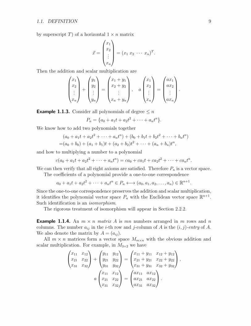
by superscript T ) of a horizontal 1× n matrix
~x =
x1
x2...xn
= (x1 x2 · · · xn)T .
Then the addition and scalar multiplication arex1
x2...xn
+
y1
y2...yn
=
x1 + y1
x2 + y2...
xn + yn
, a
x1
x2...xn
=
ax1
ax2...axn
.
Example 1.1.3. Consider all polynomials of degree ≤ n
Pn = {a0 + a1t+ a2t2 + · · ·+ ant
n}.We know how to add two polynomials together
(a0 + a1t+ a2t2 + · · ·+ ant
n) + (b0 + b1t+ b2t2 + · · ·+ bnt
n)
=(a0 + b0) + (a1 + b1)t+ (a2 + b2)t2 + · · ·+ (an + bn)tn,
and how to multiplying a number to a polynomial
c(a0 + a1t+ a2t2 + · · ·+ ant
n) = ca0 + ca1t+ ca2t2 + · · ·+ cant
n.
We can then verify that all eight axioms are satisfied. Therefore Pn is a vector space.The coefficients of a polynomial provide a one-to-one correspondence
a0 + a1t+ a2t2 + · · ·+ ant
n ∈ Pn ←→ (a0, a1, a2, . . . , an) ∈ Rn+1.
Since the one-to-one correspondence preserves the addition and scalar multiplication,it identifies the polynomial vector space Pn with the Euclidean vector space Rn+1.Such identification is an isomorphism.
The rigorous treatment of isomorphism will appear in Section 2.2.2.
Example 1.1.4. An m × n matrix A is mn numbers arranged in m rows and ncolumns. The number aij in the i-th row and j-column of A is the (i, j)-entry of A.We also denote the matrix by A = (aij).
All m × n matrices form a vector space Mm×n with the obvious addition andscalar multiplication. For example, in M3×2 we havex11 x12
x21 x22
x31 x32
+
y11 y12
y21 y22
y31 y32
=
x11 + y11 x12 + y12
x21 + y21 x22 + y22
x31 + y31 x32 + y32
,
a
x11 x12
x21 x22
x31 x32
=
ax11 ax12
ax21 ax22
ax31 ax32
.
10 CHAPTER 1. VECTOR SPACE
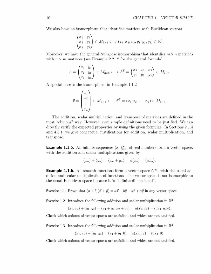
We also have an isomorphism that identifies matrices with Euclidean vectorsx1 y1
x2 y2
x3 y3
∈M3×2 ←→ (x1, x2, x3, y1, y2, y3) ∈ R6.
Moreover, we have the general transpose isomorphism that identifies m×n matriceswith n×m matrices (see Example 2.2.12 for the general formula)
A =
x1 y1
x2 y2
x3 y3
∈M3×2 ←→ AT =
(x1 x2 x3
y1 y2 y3
)∈M2×3.
A special case is the isomorphism in Example 1.1.2
~x =
x1
x2...xn
∈Mn×1 ←→ ~xT = (x1 x2 · · · xn) ∈M1×n.
The addition, scalar multiplication, and transpose of matrices are defined in themost “obvious” way. However, even simple definitions need to be justified. We candirectly verify the expected properties by using the given formulae. In Sections 2.1.4and 4.3.1, we give conceptual justifications for addition, scalar multiplication, andtranspose.
Example 1.1.5. All infinite sequences (xn)∞n=1 of real numbers form a vector space,with the addition and scalar multiplications given by
(xn) + (yn) = (xn + yn), a(xn) = (axn).
Example 1.1.6. All smooth functions form a vector space C∞, with the usual ad-dition and scalar multiplication of functions. The vector space is not isomorphic tothe usual Euclidean space because it is “infinite dimensional”.
Exercise 1.1. Prove that (a+ b)(~x+ ~y) = a~x+ b~y + b~x+ a~y in any vector space.
Exercise 1.2. Introduce the following addition and scalar multiplication in R2
(x1, x2) + (y1, y2) = (x1 + y2, x2 + y1), a(x1, x2) = (ax1, ax2).
Check which axioms of vector spaces are satisfied, and which are not satisfied.
Exercise 1.3. Introduce the following addition and scalar multiplication in R2
(x1, x2) + (y1, y2) = (x1 + y1, 0), a(x1, x2) = (ax1, 0).
Check which axioms of vector spaces are satisfied, and which are not satisfied.

1.1. DEFINITION 11
Exercise 1.4. Introduce the following addition and scalar multiplication in R2
(x1, x2) + (y1, y2) = (x1 + ky1, x2 + ly2), a(x1, x2) = (ax1, ax2).
Show that this makes R2 into a vector space if and only if k = l = 1.
Exercise 1.5. Show that all convergent sequences form a vector space.
Exercise 1.6. Show that all even smooth functions form a vector space.
Exercise 1.7. Explain that the transpose of matrix satisfies
(A+B)T = AT +BT , (cA)T = cAT , (AT )T = A.
Section 2.4.2 gives conceptual explanation of the equalities.
1.1.2 Proof by Axiom
We establish some basic properties of vector spaces. You can directly verify theseproperties in the Euclidean space. For general vector spaces, however, we shouldderive these properties from the axioms.
Proposition 1.1.2. The zero vector is unique.
Proof. Suppose ~01 and ~02 are two zero vectors. By applying the first equality inAxiom 3 to ~u = ~01 and ~0 = ~02, we get ~01 +~02 = ~01. By applying the second equalityin Axiom 3 to ~0 = ~01 and ~u = ~02, we get ~02 = ~01 +~02. Combining the two equalities,we get ~02 = ~01 +~02 = ~01.
Proposition 1.1.3. If ~u+ ~v = ~u, then ~v = ~0.
By Axioms 2, we also have ~v + ~u = ~u, then ~v = ~0. Both properties are thecancelation law.
Proof. Suppose ~u+ ~v = ~u. By Axiom 3, there is ~w, such that ~w+ ~u = ~0. We use ~winstead of ~v in the axiom, because ~v is already used in the proposition. Then
~v = ~0 + ~v (Axiom 3)
= (~w + ~u) + ~v (choice of ~w)
= ~w + (~u+ ~v) (Axiom 2)
= ~w + ~u (assumption)
= ~0. (choice of ~w)

12 CHAPTER 1. VECTOR SPACE
Proposition 1.1.4. a~u = ~0 if and only if a = 0 or ~u = ~0.
Proof. By Axioms 3, 7, 8, we have
0~u+ 0~u = (0 + 0)~u = 0~u, a~0 + a~0 = a(~0 +~0) = a~0.
Then by Proposition 1.1.3, we get 0~u = ~0 and a~0 = ~0. This proves the if part of theproposition.
The only if part means a~u = ~0 implies a = 0 or ~u = ~0. This is the same asa~u = ~0 and a 6= 0 implying ~u = ~0. So we assume a~u = ~0 and a 6= 0, and then applyAxioms 5, 6 and a~0 = ~0 (just proved) to get
~u = 1~u = (a−1a)~u = a−1(a~u) = a−1~0 = ~0.
Exercise 1.8. Directly verify Propositions 1.1.2, 1.1.3, 1.1.4 in Rn.
Exercise 1.9. Prove that the vector ~v in Axiom 4 is unique, and is (−1)~u. This justifiesthe notation −~u. Moreover, prove −(−~u) = ~u.
Exercise 1.10. Prove that a~v = b~v if and only if a = b or ~v = ~0.
Exercise 1.11. Prove the more general version of the cancelation law: ~u + ~v1 = ~u + ~v2
implies ~v1 = ~v2.
Exercise 1.12. We use Exercise 1.9 to define ~u−~v = ~u+(−~v). Prove the following properties
−(~u− ~v) = −~u+ ~v, −(~u+ ~v) = −~u− ~v.
1.2 Linear Combination
1.2.1 Linear Combination Expression
Combining addition and scalar multiplication gives linear combination
a1~v1 + a2~v2 + · · ·+ an~vn.
If we start with a nonzero seed vector ~u, then all its linear combinations a~u forma straight line passing through the origin ~0. If we start with two non-parallel vectors~u and ~v, then all their linear combinations a~u+ b~v form a plane passing through theorigin ~0. See Figure 1.2.1.
Exercise 1.13. What are all the linear combinations of two parallel vectors ~u and ~v?

1.2. LINEAR COMBINATION 13
~0
~u~v
0.5~u
1.5~u
−~u
2~u3~u~u+ ~v
2~u+ ~v
−~v ~u− ~v2~u− ~v
~u− 2~v
2~u− ~v
5~u− 4~v
−2~u+ 3~v
Figure 1.2.1: Linear combination.
By the axioms of vector spaces, we can easily verify the following
c1(a1~v1 + · · ·+ an~vn) + c2(b1~v1 + · · ·+ bn~vn)
= (c1a1~v1 + · · ·+ c1an~vn) + (c2b1~v1 + · · ·+ c2bn~vn)
= (c1a1 + c2b1)~v1 + · · ·+ (c1an + c2bn)~vn.
This show the linear combination of two linear combinations is still a linear combi-nation. The fact can be easily extended to more linear combinations.
Proposition 1.2.1. A linear combination of linear combinations is still a linearcombination.
Example 1.2.1. In R3, we try to express ~v = (10, 11, 12) as a linear combination ofthe following vectors
~v1 = (1, 2, 3), ~v2 = (4, 5, 6), ~v3 = (7, 8, 9).
This means finding suitable coefficients x1, x2, x3, such that
~v =
101112
= x1~v1 + x2~v2 + x3~v3
= x1
123
+ x2
456
+ x3
789
=
x1 + 4x2 + 7x3
2x1 + 5x2 + 8x3
3x1 + 6x2 + 9x3
.
In other words, we try to solve the system of linear equations
x1 + 4x2 + 7x3 = 10,
2x1 + 5x2 + 8x3 = 11,
3x1 + 6x2 + 9x3 = 12.

14 CHAPTER 1. VECTOR SPACE
By the way, we see the advantage of expressing Euclidean vectors in the vertical wayin calculations.
To solve the system, we may eliminate x1 in the second and third equations, byusing E2 − 2E1 (multiply the first equation by −2 and add to the second equation)and E3 − 3E1 (multiply the first equation by −3 and add to the third equation).The result of the two operations is
x1 + 4x2 + 7x3 = 10,
− 3x2 − 6x3 = −9,
− 6x2 − 12x3 = −18.
Then we use E3 − 2E2 to get
x1 + 4x2 + 7x3 = 10,
− 3x2 − 6x3 = −9,
0 = 0.
The last equation is trivial, and we only need to solve the first two equations. Wemay do −1
3E2 (multiplying −1
3to the second equation) to get
x1 + 4x2 + 7x3 = 10,
x2 + 2x3 = 3,
0 = 0.
From the second equation, we get x2 = 3−2x3. Substituting into the first equation,we get x1 = 10− 4(3− 2x3)− 7x3 = −2 + x3. The solution of the system is
x1 = −2 + x3, x2 = 3− 2x3, x3 arbitrary.
We conclude that ~v is a linear combination of ~v1, ~v2, ~v3, and there are many linearcombination expressions, i.e., the expression is not unique.
Example 1.2.2. In P2, we look for a, such that p(t) = 10 + 11t + at2 is a linearcombination of the following polynomials,
p1(t) = 1 + 2t+ 3t2, p2(t) = 4 + 5t+ 6t2, p3(t) = 7 + 8t+ 9t2,
This means finding suitable coefficients x1, x2, x3, such that
10 + 11t+ at2 = x1(1 + 2t+ 3t2) + x2(4 + 5t+ 6t2) + x3(7 + 8t+ 9t2)
= (x1 + 4x2 + 7x3) + (2x1 + 5x2 + 8x3)t+ (3x1 + 6x2 + 9x3)t2.
Comparing the coefficients of 1, t, t2, we get a system of linear equations
x1 + 4x2 + 7x3 = 10,
2x1 + 5x2 + 8x3 = 11,
3x1 + 6x2 + 9x3 = a.

1.2. LINEAR COMBINATION 15
We use the same simplification process in Example 1.2.1 to simplify the system.First we get
x1 + 4x2 + 7x3 = 10,
− 3x2 − 6x3 = −9,
− 6x2 − 12x3 = a− 30.
Then we getx1 + 4x2 + 7x3 = 10,
− 3x2 − 6x3 = −9,
0 = a− 12.
If a 6= 12, then the last equation is a contradiction, and the system has no solution.If a = 12, then we are back to Example 1.2.1, and the system has (non-unique)solution.
We conclude p(t) is a linear combination of p1(t), p2(t), p3(t) if and only if a = 12.
Exercise 1.14. Find the condition on a, such that the last vector can be expressed as alinear combination of the previous ones.
1. (1, 2, 3), (4, 5, 6), (7, a, 9), (10, 11, 12).
2. (1, 2, 3), (7, a, 9), (10, 11, 12).
3. 1 + 2t+ 3t2, 7 + at+ 9t2, 10 + 11t+ 12t2.
4. t2 + 2t+ 3, 7t2 + at+ 9, 10t2 + 11t+ 12.
5.
(1 22 3
),
(4 55 6
),
(7 aa 9
),
(10 1111 12
).
6.
(1 23 3
),
(7 a9 9
),
(10 1112 12
).
1.2.2 Row Operation
Examples 1.2.1 and 1.2.2 show that the problem of expressing a vector as a linearcombination is equivalent to solving a system of linear equations. The shape ofthe vector (Euclidean, or polynomial, or some other form) is not important for thecalculation. What is important is the coefficients in the vectors.
In general, to express a vector ~b ∈ Rm as a linear combination of ~v1, ~v2, . . . , ~vn ∈Rm, we use ~vi to form the columns of a matrix
A = (aij) =
a11 a12 · · · a1n
a21 a22 · · · a2n...
......
am1 am2 · · · amn
= (~v1 ~v2 · · · ~vn), ~vi =
a1i
a2i...ami
. (1.2.1)

16 CHAPTER 1. VECTOR SPACE
We denote the linear combination by A~x
A~x = x1~v1 + x2~v2 + · · ·+ xn~vn = x1
a11
a21...am1
+ x2
a12
a22...am2
+ · · ·+ xn
a1n
a2n...
amn
=
a11x1 + a12x2 + · · ·+ a1nxna21x1 + a22x2 + · · ·+ a2nxn
...am1x1 + am2x2 + · · ·+ amnxn
. (1.2.2)
Then the linear combination expression
A~x = x1~v1 + x2~v2 + · · ·+ xn~vn = ~b
means a system of linear equations
a11x1 + a12x2 + · · · + a1nxn = b1,
a21x1 + a22x2 + · · · + a2nxn = b2,
...
am1x1 + am2x2 + · · · + amnxn = bm.
We call A the coefficient matrix of the system, and call ~b = (b1, b2, . . . , bn) the rightside. The augmented matrix of the system is
(A~b) =
a11 a12 · · · a1n b1
a21 a22 · · · a2n b2...
......
...am1 am2 · · · amn bm
.
We have the correspondences
equations ⇐⇒ rows of (A~b),
variables ⇐⇒ columns of A.
A system of linear equations can be solved by the process of Gaussian elimina-tion, as illustrated in Examples 1.2.1 and 1.2.2. The idea is to eliminate variables,and thereby simplify equations. This is equivalent to the similar simplifications ofthe augmented matrix (A ~b). For example, the Gaussian elimination process inExample 1.2.1 corresponds to the following operations on rows1 4 7 10
2 5 8 113 6 9 12
R2−2R1R3−3R1−−−−→
1 4 7 100 −3 −6 −90 −6 −12 −18
R3−2R2
− 13R2−−−−→
1 4 7 100 1 2 30 0 0 0
. (1.2.3)
In general, we may use three types of row operations, which do not change solutionsof a system of linear equations.

1.2. LINEAR COMBINATION 17
• Ri ↔ Rj: exchange the i-th and j-th rows.
• cRi: multiply a number c 6= 0 to the i-th row.
• Ri + cRj: add the c multiple of the j-th row to the i-th row.
In Example 1.2.1, we use the third operation to create zero coefficients (and thereforesimpler matrix). We use the second operation to simplify the coefficients (say, −3is changed to 1). We may use the first operation to rearrange the equations fromthe most complicated (i.e., longest) to the simplest (i.e., shortest). We did not usethis operation in the example because the arrangement is already from the mostcomplicated to the simplest.
Example 1.2.3. We rearrange the order of vectors as ~v2, ~v3, ~v1 in Example 1.2.1.The corresponding row operations tell us how to express ~v as a linear combinationof ~v2, ~v3, ~v1. We remark that the first row operation is also used.4 7 1 10
5 8 2 116 9 3 12
R2−R1R3−R1−−−−→
4 7 1 101 1 1 12 2 2 2
R1−4R2R3−2R2−−−−→
0 3 −3 61 1 1 10 0 0 0
− 1
3R1
R1↔R2−−−−→
1 1 1 10 1 −1 20 0 0 0
R1−R2−−−−→
1 0 2 −10 1 −1 20 0 0 0
.
The system is simplified to x2 + 2x1 = −1 and x3 − x1 = 2. We get the generalsolution
x2 = −1− 2x1, x3 = 2 + x1, x1 arbitrary.
Exercise 1.15. Explain that row operations can always be reversed:
• The reverse of Ri ↔ Rj is Ri ↔ Rj .
• The reverse of cRi is c−1Ri.
• The reverse of Ri + cRj is Ri − cRj .
Exercise 1.16. Explain that row operations do not change the solutions of the correspondingsystem.
1.2.3 Row Echelon Form
We use three row operations to simplify a matrix. The simplest shape we can achieveis called the row echelon form. For the matrices in Examples 1.2.1 and 1.2.3, therow echelon form is• ∗ ∗ ∗0 • ∗ ∗
0 0 0 0
, • 6= 0, ∗ can be any number. (1.2.4)

18 CHAPTER 1. VECTOR SPACE
The entries indicated by • are called the pivots. The rows and columns containingthe pivots are pivot rows and pivot columns. In the row echelon form (1.2.4), thepivot rows are the first and second, and the pivot columns are the first and second.The following are all the 2× 3 row echelon forms(
• ∗ ∗0 • ∗
),
(• ∗ ∗0 0 •
),
(• ∗ ∗0 0 0
),
(0 • ∗0 0 •
),
(0 • ∗0 0 0
),
(0 0 •0 0 0
),
(0 0 00 0 0
).
In general, a row echelon form has the shape of upside down staircase (indicatingsimpler and simpler linear equations), and the shape is characterised by the locationsof the pivots. The pivots are the leading nonzero entries in the rows. They appearin the first several rows, and in later and later positions. The subsequent non-pivotrows are completely zero. We note that each row has at most one pivot and eachcolumn has at most one pivot. Therfore
number of pivot rows = number of pivots = number of pivot columns.
For an m × n matrix, the number above is no more than the number of rows andcolumns
number of pivots ≤ min{m,n}. (1.2.5)
Exercise 1.17. How can row operations improve the following shapes to become upsidedown staircase?
1.
0 • ∗ ∗0 0 0 0• ∗ ∗ ∗
. 2.
• ∗ ∗ ∗• ∗ ∗ ∗0 0 0 0
. 3.
0 • ∗ ∗0 • ∗ ∗• ∗ ∗ ∗
. 4.
0 • ∗ ∗0 0 • ∗• ∗ ∗ ∗
.
Then explain why the shape (1.2.4) cannot be further improved?
Exercise 1.18. Display all the 2×2 row echelon forms. How about 3×2 row echelon forms?
Exercise 1.19. How many m× n row echelon forms are there?
If a 6= 12 in Example 1.2.2, then the augmented matrix of the system has thefollowing row echelon form • ∗ ∗ ∗0 • ∗ ∗
0 0 0 •
The row (0 0 0 •) represents the equation 0 = •, a contradiction. Therefore thesystem has no solution. We remark that the row (0 0 0 •) means the last column ispivot.
1.2. LINEAR COMBINATION 19
If a = 12, then we do not have the contradiction, and the system has solution.Section 1.2.4 shows the existence of solution even more explicitly.
The discussion leads to the first part of the following.
Theorem 1.2.2. A system of linear equations A~x = ~b has solution if and only if ~bis not a pivot column of the augmented matrix (A~b). The solution is unique if andonly if all columns of A are pivot.
1.2.4 Reduced Row Echelon Form
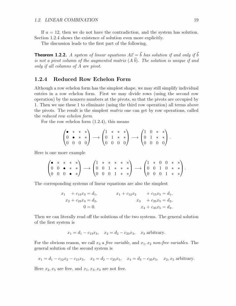
Although a row echelon form has the simplest shape, we may still simplify individualentries in a row echelon form. First we may divide rows (using the second rowoperation) by the nonzero numbers at the pivots, so that the pivots are occupied by1. Then we use these 1 to eliminate (using the third row operation) all terms abovethe pivots. The result is the simplest matrix one can get by row operations, calledthe reduced row echelon form.
For the row echelon form (1.2.4), this means• ∗ ∗ ∗0 • ∗ ∗0 0 0 0
−→1 ∗ ∗ ∗
0 1 ∗ ∗0 0 0 0
−→1 0 ∗ ∗
0 1 ∗ ∗0 0 0 0
.
Here is one more example• ∗ ∗ ∗ ∗0 0 • ∗ ∗0 0 0 • ∗
−→1 ∗ ∗ ∗ ∗ ∗
0 0 1 ∗ ∗ ∗0 0 0 1 ∗ ∗
−→1 ∗ 0 0 ∗ ∗
0 0 1 0 ∗ ∗0 0 0 1 ∗ ∗
.
The corresponding systems of linear equations are also the simplest
x1 + c13x3 = d1,
x2 + c23x3 = d2,
0 = 0.
x1 + c12x2 + c15x5 = d1,
x3 + c25x5 = d2,
x4 + c35x5 = d3.
Then we can literally read off the solutions of the two systems. The general solutionof the first system is
x1 = d1 − c13x3, x2 = d2 − c23x3, x3 arbitrary.
For the obvious reason, we call x3 a free variable, and x1, x2 non-free variables. Thegeneral solution of the second system is
x1 = d1 − c12x2 − c15x5, x3 = d2 − c25x5, x4 = d3 − c35x5, x2, x5 arbitrary.
Here x2, x5 are free, and x1, x3, x4 are not free.
20 CHAPTER 1. VECTOR SPACE
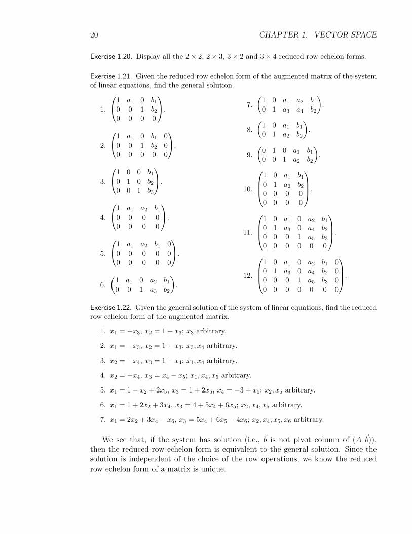
Exercise 1.20. Display all the 2× 2, 2× 3, 3× 2 and 3× 4 reduced row echelon forms.
Exercise 1.21. Given the reduced row echelon form of the augmented matrix of the systemof linear equations, find the general solution.
1.
1 a1 0 b10 0 1 b20 0 0 0
.
2.
1 a1 0 b1 00 0 1 b2 00 0 0 0 0
.
3.
1 0 0 b10 1 0 b20 0 1 b3
.
4.
1 a1 a2 b10 0 0 00 0 0 0
.
5.
1 a1 a2 b1 00 0 0 0 00 0 0 0 0
.
6.
(1 a1 0 a2 b10 0 1 a3 b2
).
7.
(1 0 a1 a2 b10 1 a3 a4 b2
).
8.
(1 0 a1 b10 1 a2 b2
).
9.
(0 1 0 a1 b10 0 1 a2 b2
).
10.
1 0 a1 b10 1 a2 b20 0 0 00 0 0 0
.
11.
1 0 a1 0 a2 b10 1 a3 0 a4 b20 0 0 1 a5 b30 0 0 0 0 0
.
12.
1 0 a1 0 a2 b1 00 1 a3 0 a4 b2 00 0 0 1 a5 b3 00 0 0 0 0 0 0
.
Exercise 1.22. Given the general solution of the system of linear equations, find the reducedrow echelon form of the augmented matrix.
1. x1 = −x3, x2 = 1 + x3; x3 arbitrary.
2. x1 = −x3, x2 = 1 + x3; x3, x4 arbitrary.
3. x2 = −x4, x3 = 1 + x4; x1, x4 arbitrary.
4. x2 = −x4, x3 = x4 − x5; x1, x4, x5 arbitrary.
5. x1 = 1− x2 + 2x5, x3 = 1 + 2x5, x4 = −3 + x5; x2, x5 arbitrary.
6. x1 = 1 + 2x2 + 3x4, x3 = 4 + 5x4 + 6x5; x2, x4, x5 arbitrary.
7. x1 = 2x2 + 3x4 − x6, x3 = 5x4 + 6x5 − 4x6; x2, x4, x5, x6 arbitrary.
We see that, if the system has solution (i.e., ~b is not pivot column of (A ~b)),then the reduced row echelon form is equivalent to the general solution. Since thesolution is independent of the choice of the row operations, we know the reducedrow echelon form of a matrix is unique.

1.3. BASIS 21
We also see the following correspondence
variables in A~x = ~b free non-freecolumns in A non-pivot pivot
In particular, the uniqueness of solution means no freedom for the variables. Bythe correspondence above, this means all columns of A are pivot. This explains thesecond part of Theorem 1.2.2.
1.3 Basis
1.3.1 Basis and Coordinate
In Example 1.2.2, we see the linear combination problem for polynomials is equiv-alent to the linear combination problem for Euclidean vectors. In Example 1.1.3, theequivalence is given by expressing polynomials as linear combinations of 1, t, t2, . . . , tn
with unique coefficients. In general, we ask for the following.
Definition 1.3.1. A ordered set α = {~v1, ~v2, . . . , ~vn} of vectors in a vector space Vis a basis of V , if for any ~x ∈ V , there exist unique x1, x2, . . . , xn, such that
~x = x1~v1 + x2~v2 + · · ·+ xn~vn.
The coefficients x1, x2, . . . , xn are the coordinates of ~x with respect to the (or-dered) basis. The unique expression means that the α-coordinate map
~x ∈ V 7→ [~x]α = (x1, x2, . . . , xn) ∈ Rn
is well defined. The reverse map is given by the linear combination
(x1, x2, . . . , xn) ∈ Rn 7→ x1~v1 + x2~v2 + · · ·+ xn~vn ∈ V.
The two way maps identify (called isomorphism) the general vector space V withthe Euclidean space Rn. Moreover, the following result shows that the coordinatepreserves linear combinations. Therefore we may use the coordinate to translatelinear algebra problems (such as linear combination expression) in a general vectorspace to corresponding problems in an Euclidean space.
Proposition 1.3.2. [~x+ ~y]α = [~x]α + [~y]α, [a~x]α = a[~x]α.
Proof. Let [~x]α = (x1, x2, . . . , xn) and [~y]α = (y1, y2, . . . , yn). Then by the definitionof coordinates, we have
~x = x1~v1 + x2~v2 + · · ·+ xn~vn, ~y = y1~v1 + y2~v2 + · · ·+ yn~vn.

22 CHAPTER 1. VECTOR SPACE
Adding the two together, we have
~x+ ~y = (x1 + y1)~v1 + (x2 + y2)~v2 + · · ·+ (xn + yn)~vn.
By the definition of coordinates, this means
[~x+ ~y]α = (x1 + y1, x2 + y2, . . . , xn + yn)
= (x1, x2, . . . , xn) + (y1, y2, . . . , yn) = [~x]α + [~y]α.
The proof of [a~x]α = a[~x]α is similar.
Example 1.3.1. The standard basis vector ~ei in Rn has the i-th coordinate 1 andall other coordinates 0. For example, the standard basis vectors of R3 are
~e1 = (1, 0, 0), ~e2 = (0, 1, 0), ~e3 = (0, 0, 1).
By the equality(x1, x2, . . . , xn) = x1~e1 + x2~e2 + · · ·+ xn~en,
any vector is a linear combination of the standard basis vectors. Moreover, theequality shows that, if two expressions on the right are equal
x1~e1 + x2~e2 + · · ·+ xn~en = y1~e1 + y2~e2 + · · ·+ yn~en,
then the two vectors are also equal
(x1, x2, . . . , xn) = (y1, y2, . . . , yn).
Of course this means exactly x1 = y1, x2 = y2, . . . , xn = yn, i.e., the uniqueness ofthe coefficients. Therefore the standard basis vectors for the standard basis ε ={~e1, ~e2, . . . , ~en} of Rn. The equality can be interpreted as
[~x]ε = ~x.
If we change the order in the standard basis, then we should also change theorder of coordinates
[(x1, x2, x3)]{~e1,~e2,~e3} = (x1, x2, x3),
[(x1, x2, x3)]{~e2,~e1,~e3} = (x2, x1, x3),
[(x1, x2, x3)]{~e3,~e2,~e1} = (x3, x2, x1).
Example 1.3.2. Any polynomial of degree ≤ n is of the form
p(t) = a0 + a1t+ a2t2 + · · ·+ ant
n.
The formula can be interpreted as that p(t) is a linear combination of monomials1, t, t2, . . . , tn. For the uniqueness of the linear combination, we consider the equality
a0 + a1t+ a2t2 + · · ·+ ant
n = b0 + b1t+ b2t2 + · · ·+ bnt
n.

1.3. BASIS 23
The equality usually mean equal functions. In other words, if we substitute anyreal number in place of t, the two sides have the same value. Taking t = 0, we geta0 = b0. Dividing the remaining equality by t 6= 0, we get
a1 + a2t+ · · ·+ antn−1 = b1 + b2t+ · · ·+ bnt
n−1 for t 6= 0.
Taking limt→0 on both sides, we get a1 = b1. Inductively, we find that ai = bi forall i. This shows the uniqueness of the linear combination. Therefore 1, t, t2, . . . , tn
form a basis of Pn. We have
[a0 + a1t+ a2t2 + · · ·+ ant
n]{1,t,t2,...,tn} = (a0, a1, a2, . . . , an).
Example 1.3.3. Consider the monomials 1, t− 1, (t− 1)2 at t0 = 1. Any quadraticpolynomial is a linear combination of 1, t− 1, (t− 1)2
a0 + a1t+ a2t2 = a0 + a1[1 + (t− 1)] + a2[1 + (t− 1)]2
= (a0 + a1 + a2) + (a1 + 2a2)(t− 1) + a2(t− 1)2.
Moreover, if two linear combinations are equal
a0 + a1(t− 1) + a2(t− 1)2 = b0 + b1(t− 1) + b2(t− 1)2,
then substituting t by t+ 1 gives the equality
a0 + a1t+ a2t2 = b0 + b1t+ b2t
2.
This means a0 = b0, a1 = b1, a2 = b2, or the uniqueness of the linear combinationexpression. Therefore 1, t − 1, (t − 1)2 form a basis of P2. In general, 1, t − t0, (t −t0)2, . . . , (t− t0)n form a basis of Pn.
Exercise 1.23. Show that the following 3 × 2 matrices form a basis of the vector spaceM3×2. 1 0
0 00 0
,
0 01 00 0
,
0 00 01 0
,
0 10 00 0
,
0 00 10 0
,
0 00 00 1
.
In general, how many matrices are in a basis of the vector space Mm×n of m×n matrices?
Exercise 1.24. For an ordered basis α = {~v1, ~v2, . . . , ~vn} is of V , explain that [~vi]α = ~ei.
Exercise 1.25. A permutation of {1, 2, . . . , n} is a one-to-one correspondence π : {1, 2, . . . , n} →{1, 2, . . . , n}. Let α = {~v1, ~v2, . . . , ~vn} be a basis of V .
1. Show that π(α) = {~vπ(1), ~vπ(2), . . . , ~vπ(n)} is still a basis.
2. What is the relation between [~x]α and [~x]π(α)?

24 CHAPTER 1. VECTOR SPACE
1.3.2 Spanning Set
The definition of basis consists of two parts, the existence of linear combinationexpression for all vectors, and the uniqueness of the expression. We study the twoproperties separately. The existence is the following property.
Definition 1.3.3. A set of vectors α = {~v1, ~v2, . . . , ~vn} in a vector space V spans Vif any vector in V can be expressed as a linear combination of ~v1, ~v2, . . . , ~vn.
For V = Rm, we form the m × n matrix A = (~v1 ~v2 · · ·~vn). Then the vectorsspanning V means the system of linear equations
A~x = x1~v1 + x2~v2 + · · ·+ xn~vn = ~b
has solution for all right side ~b.
Example 1.3.4. For ~u = (a, b) and ~v = (c, d) to span R2, we need the system of twolinear equations to have solution for all p, q
ax+ cy = p,
bx+ dy = q.
We multiply the first equation by b and the second equation by a, and then subtractthe two. We get
(bc− ad)y = bp− aq.If ad 6= bc, then we can solve for y. We may further substitute y into the originalequations to get x. Therefore the system has solution for all p, q.
We conclude that (a, b) and (c, d) span R2 in case ad 6= bc. For example, by1 · 4 6= 3 · 2, we know (1, 2) and (3, 4) span R2.
Exercise 1.26. Show that a linear combination of (1, 2) and (2, 4) is always of the form(a, 2a). Then explain that the two vectors do not span R2.
Exercise 1.27. Explain that, if ad = bc, then (a, b) and (c, d) do not span R2.
Example 1.3.5. The following vectors span R3
~v1 = (1, 2, 3), ~v2 = (4, 5, 6), ~v3 = (7, 8, 9),
if and only if (~v1 ~v2 ~v3)~x = ~b has solution for all~b. We apply the same row operationsin (1.2.3) to the augmented matrix
(~v1 ~v2 ~v3~b) =
1 4 7 b1
2 5 8 b2
3 6 9 b3
→1 4 7 b′1
0 1 2 b′20 0 0 b′3
.

1.3. BASIS 25
Although we may calculate the explicit formulae for b′i, which are linear combinationsof b1, b2, b3, we do not need these. All we need to know is that, since b1, b2, b3 arearbitrary, and the row operations can be reversed (see Exercise 1.15), the right sideb′1, b
′2, b′3 in the row echelon form are also arbitrary. In particular, it is possible to
have b′3 6= 0, and the system has no solution. Therefore the three vectors do notspan R3.
If we change the third vector to ~v3 = (7, 8, a), then the same row operations give
(~v1 ~v2 ~v3~b) =
1 4 7 b1
2 5 8 b2
3 6 a b3
→1 4 7 b′1
0 1 2 b′20 0 a− 9 b′3
.
If a 6= 9, then the last column is not pivot. By Theorem 1.2.2, the system alwayshas solution. Therefore (1, 2, 3), (4, 5, 6), (7, 8, a) span R3 if and only if a 6= 9.
Example 1.3.5 can be summarized as the following criterion for a set of vectorsto span the Euclidean space.
Proposition 1.3.4. Let α = {~v1, ~v2, . . . , ~vn} ⊂ Rm and A = (~v1 ~v2 · · · ~vn). Thefollowing are equivalent.
1. α spans Rm.
2. A~x = ~b has solution for all ~b ∈ Rm.
3. All rows of A are pivot. In other words, the row echelon form of A has no zerorow (0 0 · · · 0).
Moreover, we have m ≤ n in the above cases.
For the last property n ≥ m, we note that all rows pivot implies the number ofpivots is m. Then by (1.2.5), we get m ≤ min{m,n} ≤ n.
Example 1.3.6. To find out whether (1, 2, 3), (4, 5, 6), (7, 8, a), (10, 11, b) span R3,we apply the row operations in (1.2.3)1 4 7 10
2 5 8 113 6 a b
→1 4 7 10
0 1 2 30 0 a− 9 b− 12
.
The row echelon form depends on the values of a and b. If a 6= 9, then the result isalready a row echelon form • ∗ ∗ ∗0 • ∗ ∗
0 0 • ∗
.
26 CHAPTER 1. VECTOR SPACE
If a = 9, then the result is • ∗ ∗ ∗0 • ∗ ∗0 0 0 b− 12
.
Then we have two possible row echelon forms• ∗ ∗ ∗0 • ∗ ∗0 0 0 •
for b 6= 12;
• ∗ ∗ ∗0 • ∗ ∗0 0 0 0
for b = 12.
By Proposition 1.3.4, the vectors (1, 2, 3), (4, 5, 6), (7, 8, a), (10, 11, b) span R3 if andonly if a 6= 9, or a = 9 and b 6= 12.
If we restrict the row operations to the first three columns, then we find that allrows are pivot if and only if a 6= 9. Therefore the first three vectors span R3 if andonly if a 6= 9.
We may also restrict the row operations to the first, second and fourth columns,and find that all rows are pivot if and only if b 6= 12. This is the condition for(1, 2, 3), (4, 5, 6), (10, 11, b) to span R3.
Exercise 1.28. Find row echelon form and determine whether the column vectors span theEuclidean space.
1.
1 2 3 12 3 1 23 1 2 3
.
2.
1 2 32 3 13 1 21 2 3
.
3.
1 2 32 3 43 4 5
.
4.
1 2 3 42 3 4 53 4 5 a
.
5.
1 2 32 3 43 4 54 5 a
.
6.
0 2 −1 4−1 3 0 12 −4 −1 21 1 −2 7
.
7.
1 0 0 10 1 1 01 0 1 00 1 0 1
.
8.
1 0 0 10 1 1 01 0 1 a0 1 a b
.
Exercise 1.29. If ~v1, ~v2, . . . , ~vn span V , prove that ~v1, ~v2, . . . , ~vn, ~w span V .The property means that any set bigger than a spanning set is also a spanning set.
Exercise 1.30. Suppose ~w is a linear combination of ~v1, ~v2, . . . , ~vn. Prove that ~v1, ~v2, . . . , ~vn, ~wspan V if and only if ~v1, ~v2, . . . , ~vn span V .
The property means that, if one vector is a linear combination of the others, then wemay remove the vector without changing the spanning set property.
Exercise 1.31. Suppose ~v1, ~v2, . . . , ~vn ∈ V . If each of ~w1, ~w2, . . . , ~wm is a linear combinationof ~v1, ~v2, . . . , ~vn, and ~w1, ~w2, . . . , ~wm span V , prove that ~v1, ~v2, . . . , ~vn also span V .
Exercise 1.32. Prove that the following are equivalent for a set of vectors in V .
1. ~v1, . . . , ~vi, . . . , ~vj , . . . , ~vn span V .

1.3. BASIS 27
2. ~v1, . . . , ~vj , . . . , ~vi, . . . , ~vn span V .
3. ~v1, . . . , c~vi, . . . , ~vn, c 6= 0, span V .
4. ~v1, . . . , ~vi + c~vj , . . . , ~vj , . . . , ~vn span V .
Example 1.3.7. By the last part of Proposition 1.3.4, three vectors (1, 0,√
2, π),(log 2, e, 100,−0.5), (
√3, e−1, sin 1, 2.3) cannot span R4.
Exercise 1.33. If m > n in Proposition 1.3.4, what can you conclude?
Exercise 1.34. Explain that the vectors do not span the Euclidean space. Then interpretthe result in terms of systems of linear equations.
1. (10,−2, 3, 7, 2), (0, 8,−2, 5,−4), (8,−9, 3, 6, 5).
2. (10,−2, 3, 7, 2), (0, 8,−2, 5,−4), (8,−9, 3, 6, 5), (7,−9, 3,−5, 6).
3. (0,−2, 3, 7, 2), (0, 8,−2, 5,−4), (0,−9, 3, 6, 5), (0,−5, 4, 2,−7), (0, 4,−1, 3,−6).
4. (6,−2, 3, 7, 2), (−4, 8,−2, 5,−4), (6,−9, 3, 6, 5), (8,−5, 4, 2,−7), (−2, 4,−1, 3,−6).
1.3.3 Linear Independence
Definition 1.3.5. A set of vectors ~v1, ~v2, . . . , ~vn are linearly independent if the coef-ficients in linear combination are unique
x1~v1+x2~v2+· · ·+xn~vn = y1~v1+y2~v2+· · ·+yn~vn =⇒ x1 = y1, x2 = y2, . . . , xn = yn.
The vectors are linearly dependent if they are not linearly independent.
For V = Rm, we form the matrix A = (~v1 ~v2 · · ·~vn). Then the linear indepen-dence of the column vectors means the solution of the system of linear equations
A~x = x1~v1 + x2~v2 + · · ·+ xn~vn = ~b
is unique. By Theorem 1.2.2, we have the following criterion for linear independence.
Proposition 1.3.6. Let α = {~v1, ~v2, . . . , ~vn} ⊂ Rm and A = (~v1 ~v2 · · · ~vn). Thefollowing are equivalent.
1. α is linearly independent.
2. The solution of A~x = ~b is unique.
3. All columns of A are pivot.
Moreover, we have m ≥ n in the above cases.

28 CHAPTER 1. VECTOR SPACE
For the last property m ≥ n, we note that all columns pivot implies the numberof pivots is n. Then by (1.2.5), we get n ≤ min{m,n} ≤ m.
Example 1.3.8. We try to find the condition on a, such that
~v1 = (1, 2, 3, 4), ~v2 = (5, 6, 7, 8), ~v3 = (9, 10, 11, a)
are linearly independent. We carry out the row operations
(~v1 ~v2 ~v3) =
1 5 92 6 103 7 114 8 a
R4−R3R3−R2R2−R1−−−−→
1 5 91 1 11 1 11 1 a− 11
R1−R2R3−R2R4−R2−−−−→
0 4 81 1 10 0 00 0 a− 12
R1↔R2R3↔R4−−−−→
1 1 10 4 80 0 a− 120 0 0
.
We find all three columns are pivot if and only if a 6= 12. This is the condition forthe three vectors to be linearly independent.
Exercise 1.35. Determine the linear independence of the column vectors in Exercises 1.28.
Exercise 1.36. Prove that the following are equivalent.
1. ~v1, . . . , ~vi, . . . , ~vj , . . . , ~vn are linearly independent.
2. ~v1, . . . , ~vj , . . . , ~vi, . . . , ~vn are linearly independent.
3. ~v1, . . . , c~vi, . . . , ~vn, c 6= 0, are linearly independent.
4. ~v1, . . . , ~vi + c~vj , . . . , ~vj , . . . , ~vn are linearly independent.
Example 1.3.9. By the last part of Proposition 1.3.6, four vectors (1, log 2,√
3),(0, e, e−1), (
√2, 100, sin 1), (π,−0.5, 2.3) in R3 are linearly dependent.
Exercise 1.37. If m < n in Proposition 1.3.6, what can you conclude?
Exercise 1.38. Explain that the vectors are linearly dependent. Then interpret the resultin terms of systems of linear equations.
1. (1, 2, 3), (2, 3, 1), (3, 1, 2), (1, 3, 2), (3, 2, 1), (2, 1, 3).
2. (1, 3, 2,−4), (10,−2, 3, 7), (0, 8,−2, 5), (8,−9, 3, 6), (7,−9, 3,−5).
3. (1, 3, 2,−4), (10,−2, 3, 7), (0, 8,−2, 5), (π, 3π, 2π,−4π).
4. (1, 3, 2,−4, 0), (10,−2, 3, 7, 0), (0, 8,−2, 5, 0), (8,−9, 3, 6, 0), (7,−9, 3,−5, 0).

1.3. BASIS 29
The criterion for linear independence in Proposition 1.3.6 does not depend onthe right side. This means we only need to verify the uniqueness for the case ~b = ~0.We call the corresponding system A~x = ~0 homogeneous. The homogeneous systemalways has the zero solution ~x = ~0. Therefore we only need to ask the uniquenessof the solution of A~x = ~0.
The relation between the uniqueness for A~x = ~b and the uniqueness for A~x = ~0holds in general vector space.
Proposition 1.3.7. A set of vectors ~v1, ~v2, . . . , ~vn are linearly independent if andonly if
x1~v1 + x2~v2 + · · ·+ xn~vn = ~0 =⇒ x1 = x2 = · · · = xn = 0.
Proof. The property in the proposition is the special case of y1 = · · · = yn = 0 inthe definition of linear independence. Conversely, if the special case holds, then
x1~v1 + x2~v2 + · · ·+ xn~vn = y1~v1 + y2~v2 + · · ·+ yn~vn
=⇒ (x1 − y1)~v1 + (x2 − y2)~v2 + · · ·+ (xn − yn)~vn = ~0
=⇒ x1 − y1 = x2 − y2 = · · · = xn − yn = 0.
Example 1.3.10. By Proposition 1.3.7, a single vector ~v is linearly independent ifand only if a~v = ~0 implies a = 0. By Proposition 1.1.4, the property means exactly~v 6= ~0.
Example 1.3.11. To show that cos t, sin t, et are linearly independent, we only needto verify that the equality x1 cos t+ x2 sin t+ x3e
t = 0 implies x1 = x2 = x3 = 0.If the equality holds, then by evaluating at t = 0, π
2, π, we get
x1 + x3 = 0, x2 + x3eπ2 = 0, −x1 + x3e
π = 0.
Adding the first and third equations together, we get x3(1 + eπ) = 0. This impliesx3 = 0. Substituting x3 = 0 to the first and second equations, we get x1 = x2 = 0.
Example 1.3.12. To show t(t− 1), t(t− 2), (t− 1)(t− 2) are linearly independent,we onsider
a1t(t− 1) + a2t(t− 2) + a3(t− 1)(t− 2) = 0.
Since the equality holds for all t, we may take t = 0 and get a3(−1)(−2) = 0.Therefore a3 = 0. Similarly, by taking t = 1 and t = 2, we get a2 = 0 and a1 = 0.
In general, suppose t0, t1, . . . , tn are distinct, and1
pi(t) =∏j 6=i
(t− tj) = (t− t0)(t− t1) · · · (t− ti) · · · (t− tn)
1The notation ? is the mathematical convention that the term ? is missing.

30 CHAPTER 1. VECTOR SPACE
is the product of all t − t∗ except t − ti. Then p0(t), p(1(t), . . . , pn(t) are linearlyindependent.
Exercise 1.39. For a 6= b, show that eat and ebt are linearly independent. What about eat,ebt and ect?
Exercise 1.40. Prove that cos t, sin t, et do not span the vector space of all smooth functions,by showing that the constant function 1 is not a linear combination of the three functions.
Hint: Take several values of t in x1 cos t + x2 sin t + x3et = 1 and then derive contra-
diction.
Exercise 1.41. Determine whether the given functions are linearly independent, and whetherf(x), g(t) can be expressed as linear combinations of given functions.
1. cos2 t, sin2 t. f(t) = 1, g(t) = t.
2. cos2 t, sin2 t, 1. f(t) = cos 2t, g(t) = t.
3. 1, t, et, tet. f(t) = (1 + t)et, g(t) = f ′(t).
4. cos2 t, cos 2t. f(t) = a, g(t) = a+ sin2 t.
The following result says that linear dependence means some vector is a “waste”.The proof makes use of division by nonzero number.
Proposition 1.3.8. A set of vectors are linearly dependent if and only if one vectoris a linear combination of the other vectors.
Proof. If ~v1, ~v2, . . . , ~vn are linearly dependent, then by Proposition 1.3.7, we havex1~v1 + x2~v2 + · · ·+ xn~vn = ~0, with some xi 6= 0. Then we get
~vi = −x1
xi~v1 − · · · −
xi−1
xi~vi−1 −
xi+1
xi~vi+1 − · · · −
xnxi~vn.
This shows that the i-th vector is a linear combination of the other vectors.Conversely, if
~vi = x1~v1 + · · ·+ xi−1~vi−1 + xi+1~vi+1 + · · ·+ xn~vn,
then the left side is a linear combination with coefficients (0, . . . , 0, 1(i), 0, . . . , 0),and the right side has coefficients (x1, . . . , xi−1, 0(i), xi+1, . . . , xn). Since coefficientsare different, by definition, the vectors are linearly dependent.
Example 1.3.13. By Proposition 1.3.8, two vectors ~u and ~v are linearly dependent if andonly if either ~u is a linear combination of ~v, or ~v is a linear combination of ~u. In otherwords, the two vectors are parallel.
Two vectors are linearly independent if and only if they are not parallel.

1.3. BASIS 31
Exercise 1.42. Prove that ~v1, ~v2, . . . , ~vn, ~w are linearly independent if and only if ~v1, ~v2, . . . , ~vnare linearly independent, and ~w is not a linear combination of ~v1, ~v2, . . . , ~vn.
The property implies that any subset of a linearly independent set is also linearlyindependent. What does this tell you about linear dependence?
Exercise 1.43. Prove that ~v1, ~v2, . . . , ~vn are linearly dependent if and only if some ~vi is alinear combination of the previous vectors ~v1, ~v2, . . . , ~vi−1.
1.3.4 Minimal Spanning Set
Basis has two aspects, span and linear independence. If we already know that somevectors span a vector space, then we can achieve linear independence (and thereforebasis) by deleting “unnecessary” vectors.
Definition 1.3.9. A vector space is finite dimensional if it is spanned by finitelymany vectors.
Theorem 1.3.10. In a finite dimensional vector space, a set of vectors is a basis ifand only if it is a minimal spanning set. Moreover, any finite spanning set containsa minimal spanning set and therefore a basis.
By a minimal spanning set α, we mean α spans V , and any subset strictly smallerthan α does not span V .
Proof. Suppose α = {~v1, ~v2, . . . , ~vn} spans V . The set α is either linearly indepen-dent, or linearly dependent.
If α is linearly independent, then it is a basis by definition. Moreover, by Proposi-tion 1.3.8, we know ~vi is not a linear combination of ~v1, · · · , ~vi−1, ~vi+1 . . . , ~vn. There-fore after deleting ~vi, the remaining vectors ~v1, · · · , ~vi−1, ~vi+1 . . . , ~vn do not span V .This proves that α is a minimal spanning set.
If α is linearly dependent, then by Proposition 1.3.8, we may assume ~vi is a linearcombination of
α′ = α− {~vi} = {~v1, · · · , ~vi−1, ~vi+1 . . . , ~vn}.
By Proposition 1.2.1 (also see Exercise 1.30), linear combinations of α are also linearcombinations of α′. Therefore we get a strictly smaller spanning set α′. Then we mayask whether α′ is linearly dependent. If the answer is yes, then α′ contains strictlysmaller spanning set. The process continues and, since α is finite, will stop afterfinitely many steps. By the time we stop, we get a linearly independent spanningset. By definition, this is a basis.
We proved that “independence =⇒ minimal” and “dependence =⇒ notminimal”. This implies that “independence ⇐⇒ minimal”. Since a spanning setis independent if and only if it is a basis, we get the first part of the theorem. Thenthe second part is contained in the proof above in case α is linearly dependent.
32 CHAPTER 1. VECTOR SPACE
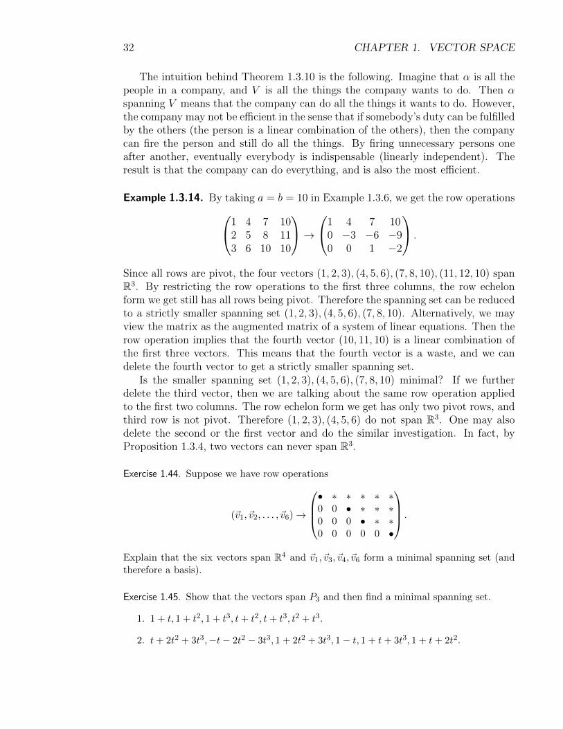
The intuition behind Theorem 1.3.10 is the following. Imagine that α is all thepeople in a company, and V is all the things the company wants to do. Then αspanning V means that the company can do all the things it wants to do. However,the company may not be efficient in the sense that if somebody’s duty can be fulfilledby the others (the person is a linear combination of the others), then the companycan fire the person and still do all the things. By firing unnecessary persons oneafter another, eventually everybody is indispensable (linearly independent). Theresult is that the company can do everything, and is also the most efficient.
Example 1.3.14. By taking a = b = 10 in Example 1.3.6, we get the row operations1 4 7 102 5 8 113 6 10 10
→1 4 7 10
0 −3 −6 −90 0 1 −2
.
Since all rows are pivot, the four vectors (1, 2, 3), (4, 5, 6), (7, 8, 10), (11, 12, 10) spanR3. By restricting the row operations to the first three columns, the row echelonform we get still has all rows being pivot. Therefore the spanning set can be reducedto a strictly smaller spanning set (1, 2, 3), (4, 5, 6), (7, 8, 10). Alternatively, we mayview the matrix as the augmented matrix of a system of linear equations. Then therow operation implies that the fourth vector (10, 11, 10) is a linear combination ofthe first three vectors. This means that the fourth vector is a waste, and we candelete the fourth vector to get a strictly smaller spanning set.
Is the smaller spanning set (1, 2, 3), (4, 5, 6), (7, 8, 10) minimal? If we furtherdelete the third vector, then we are talking about the same row operation appliedto the first two columns. The row echelon form we get has only two pivot rows, andthird row is not pivot. Therefore (1, 2, 3), (4, 5, 6) do not span R3. One may alsodelete the second or the first vector and do the similar investigation. In fact, byProposition 1.3.4, two vectors can never span R3.
Exercise 1.44. Suppose we have row operations
(~v1, ~v2, . . . , ~v6)→
• ∗ ∗ ∗ ∗ ∗0 0 • ∗ ∗ ∗0 0 0 • ∗ ∗0 0 0 0 0 •
.
Explain that the six vectors span R4 and ~v1, ~v3, ~v4, ~v6 form a minimal spanning set (andtherefore a basis).
Exercise 1.45. Show that the vectors span P3 and then find a minimal spanning set.
1. 1 + t, 1 + t2, 1 + t3, t+ t2, t+ t3, t2 + t3.
2. t+ 2t2 + 3t3,−t− 2t2 − 3t3, 1 + 2t2 + 3t3, 1− t, 1 + t+ 3t3, 1 + t+ 2t2.
1.3. BASIS 33
1.3.5 Maximal Independent Set
If we already know that some vectors are linearly independent, then we can achievethe span property (and therefore basis) by adding “independent” vectors. Thereforewe have two ways of constructing basis
span vector spacedelete vectors−−−−−−−→ basis
add vectors←−−−−−− linearly independent
Using the analogy of company, linear independence means there is no waste.What we need to achieve is to do all the things the company wants to do. If there isa job that the existing employees cannot do, then we need to hire somebody who cando the job. The new hire is linearly independent of the existing employees becausethe person can do something the others cannot do. We keep adding new necessarypeople until the company can do all the things, and therefore achieve the span.
Theorem 1.3.11. In a finite dimensional vector space, a set of vectors is a basis ifand only if it is a maximal linearly independent set. Moreover, any linearly inde-pendent set can be extended to a maximal linearly independent set and therefore abasis.
By a maximal linearly independent set α, if α is linearly independent, and anyset strictly bigger than α is linearly dependent.
Proof. Suppose α = {~v1, ~v2, . . . , ~vn} is a linearly independent set in V . The set αeither spans V , or does not span V .
If α spans V , then it is a basis by definition. Moreover, any vector ~v ∈ V is alinear combination of α. By Proposition 1.3.8, adding ~v to α makes the set linearlydependent. Therefore α is a maximal linearly independent set.
If α does not span V , then there is a vector ~v ∈ V which is not a linear com-bination of α. If α′ = α ∪ {~v} = {~v1, ~v2, . . . , ~vn, ~v} is linearly dependent, then byProposition 1.3.7, we have
a1~v1 + a2~v2 + · · ·+ an~vn + a~v = ~0,
and some coefficients are nonzero. If a = 0, then some of a1, a2, . . . , an are nonzero.By Proposition 1.3.7, this contradicts the linear independence of α. If a 6= 0, thenwe get
~v = −a1
a~v1 −
a2
a~v2 + · · · − an
a~vn,
contradicting the assumption that ~v is not a linear combination of α. This provesthat α′ is a linearly independent set strictly bigger than α.
Now we may ask whether α′ spans V . If the answer is no, then we can enlarge α′
further by adding another vector that is not a linear combination of α′. The resultis again a bigger linearly independent set. The process continues, and must stopafter finitely many steps due to the finite dimension assumption (full justification by

34 CHAPTER 1. VECTOR SPACE
Proposition 1.3.13). By the time we stop, we get a linearly independent spanningset, which is a basis by definition.
We proved that “span V =⇒ maximal” and “not span V =⇒ not maximal”.This implies that “span V ⇐⇒ maximal”. Since a linearly independent set spansthe vector space if and only if it is a basis, we get the first part of the theorem. Thenthe second part is contained in the proof above in case α does not span V .
Example 1.3.15. We take the transpose of the matrix in Example 1.3.14, and carryout row operations (this is the column operations on the earlier matrix)
1 2 34 5 67 8 1011 12 10
R4−R3R3−R2R2−R1−−−−→
1 2 33 3 33 3 43 3 0
R3−R2R4−R2−−−−→
1 2 33 3 30 0 10 0 −3
R2−3R1R4+3R3−−−−→
1 2 30 −3 −60 0 10 0 0
.
By Proposition 1.3.6, this shows that (1, 4, 7, 11), (2, 5, 8, 12), (3, 6, 10, 10) are linearlyindependent. However, since the last row is not pivot (or the last part of Proposition1.3.4), the three vectors do not span R4.
To enlarge the linearly independent set of three vectors, we try to add a vectorso that the same row operations produces (0, 0, 0, 1). The vector can be obtainedby reversing the operations on (0, 0, 0, 1)
0001
R2+R1R3+R2R4+R3←−−−−
0001
R4+R2R3+R2←−−−−
0001
R4−3R3R2+3R1←−−−−
0001
.
Then we have row operations1 2 3 04 5 6 07 8 10 011 12 10 1
−→
1 2 3 00 −3 −6 00 0 1 00 0 0 1
.
This shows that (1, 4, 7, 11), (2, 5, 8, 12), (3, 6, 10, 10), (0, 0, 0, 1) form a basis.If we try a more interesting vector (4, 3, 2, 1)
4193646
R2+R1R3+R2R4+R3←−−−−
4151710
R4+R2R3+R2←−−−−
4152−5
R4−3R3R2+3R1←−−−−
4321
,
then we find that (1, 4, 7, 11), (2, 5, 8, 12), (3, 6, 10, 10), (4, 19, 36, 46) form a basis.
Exercise 1.46. For the column vectors in Exercise 1.28, find a linearly independent subset,and then extend to a basis. Note that the linearly independent subset should be as big aspossible, to avoid the lazy choice such as picking the first column only.

1.3. BASIS 35
Exercise 1.47. Explain that t2(t−1), t(t2−1), t2−4 are linearly independent. Then extendto a basis of P3.
1.3.6 Dimension
Let V be a finite dimensional vector space. By Theorem 1.3.10, V has a basisα = {~v1, ~v2, . . . , ~vn}. Then the coordinate with respect to α translates the linearalgebra of V to the Euclidean space [·]α : V ↔ Rn.
Let β = {~w1, ~w2, . . . , ~wk} be another basis of V . Then the α-coordinate translatesβ into a basis [β]α = {[~w1]α, [~w2]α, . . . , [~wk]α} of Rn. Therefore [β]α (a set of kvectors) spans Rn and is also linearly independent. By the last parts of Propositions1.3.4 and 1.3.6, we get k = n. This shows that the following concept is well defined.
Definition 1.3.12. The dimension of a (finite dimensional) vector space is the num-ber of vectors in a basis.
We denote the dimension by dimV . By Examples 1.3.1, 1.3.2, and Exercise 1.23,we have dimRn = n, dimPn = n+ 1, dimMm×n = mn.
If dimV = m, then V can be identified with the Euclidean space Rm, and thelinear algebra in V is the same as the linear algebra in Rm. For example, we maychange Rm in Propositions 1.3.4 and 1.3.6 to any vector space V of dimension m,and get the following.
Proposition 1.3.13. Suppose V is a finite dimensional vector space.
1. If n vectors span V , then dimV ≤ n.
2. If n vectors in V are linearly independent, then dimV ≥ n.
Continuation of the proof of Theorem 1.3.11. The proof of the theorem creates big-ger and bigger linearly independent sets of vectors. By Proposition 1.3.13, however,the set is no longer linearly independent when the number of vectors is > dimV .This means that, if the set α we start with has n vectors, then the construction inthe proof stops after at most dimV − n steps.
We note that the argument uses Theorem 1.3.10, for the existence of basis andthen the concept of dimension. What we want to prove is Theorem 1.3.11, which isnot used in the argument.
Exercise 1.48. Explain that the vectors do not span the vector space.
1. 3 +√
2t− πt2 − 3t3, e+ 100t+ 2√
3t2, 4πt− 15.2t2 + t3.
2.
(3 84 9
),
(2 86 5
),
(4 75 0
).

36 CHAPTER 1. VECTOR SPACE
3.
(π√
31 2π
),
(√2 π
−10 2√
2
),
(3 100−77 6
),
(sin 2 π√
2π 2 sin 2
).
Exercise 1.49. Explain that the vectors are linearly dependent.
1. 3 +√
2t− πt2, e+ 100t+ 2√
3t2, 4πt− 15.2t2,√π + e2t2.
2.
(3 84 9
),
(2 86 5
),
(1 0−2 4
).
3.
(π√
31 2π
),
(√2 π
−10 2√
2
),
(3 100−77 6
),
(sin 2 π√
2π 2 sin 2
).
Theorem 1.3.14. Suppose α is a collection of vectors in a finite dimensional vectorspace V . Then any two of the following imply the third.
1. The number of vectors in α is dimV .
2. α spans V .
3. α is linearly independent.
To prove the theorem, we may translate into Euclidean space. Then by Propo-sitions 1.3.4 and 1.3.6, we only need to prove the following properties about systemof linear equations.
Theorem 1.3.15. Suppose A is an m × n matrix. Then any two of the followingimply the third.
1. m = n.
2. A~x = ~b has solution for all ~b.
3. The solution of A~x = ~b is unique.
Proof. If the second and third statement hold, then by Propositions 1.3.4 and 1.3.6,we have m ≤ n and m ≥ n. Therefore the first statement holds.
Now we assume the first statement, and prove that the second and third areequivalent. The first statement means A is an n× n matrix. By Proposition 1.3.4,the second statement means all rows are pivot, i.e., the number of pivots is n. ByProposition 1.3.6, the third statement means all columns are pivot, i.e., the numberof pivots is n. Therefore the two statements are the same.
Example 1.3.16. By Example 1.3.8, the three quadratic polynomials t(t− 1), t(t−2), (t − 1)(t − 2) are linearly independent. By Theorem 1.3.14 and dimP2 = 3, weknow the three vectors form a basis of P2.
For the general discussion, see Example 2.2.13.

1.3. BASIS 37
Exercise 1.50. Use Theorem 1.3.10 to give another proof of the first part of Proposition1.3.13. Use Theorem 1.3.11 to give another proof of the second part of Proposition 1.3.13.
Exercise 1.51. Suppose the number of vectors in α is dimV . Explain the following areequivalent.
1. α spans V .
2. α is linearly independent.
3. α is a basis.
Exercise 1.52. Show that the vectors form a basis.
1. (1, 1, 0), (1, 0, 1), (0, 1, 1) in R3.
2. (1, 1,−1), (1,−1, 1), (−1, 1, 1) in R3.
3. (1, 1, 1, 0), (1, 1, 0, 1), (1, 0, 1, 1), (0, 1, 1, 1) in R4.
Exercise 1.53. Show that the vectors form a basis.
1. 1 + t, 1 + t2, t+ t2 in P2.
2.
(1 11 0
),
(1 10 1
),
(1 01 1
),
(0 11 1
)in M2×2.
Exercise 1.54. For which a do the vectors form a basis?
1. (1, 1, 0), (1, 0, 1), (0, 1, a) in R3.
2. (1,−1, 0), (1, 0,−1), (0, 1, a) in R3.
3. (1, 1, 1, 0), (1, 1, 0, 1), (1, 0, 1, 1), (0, 1, 1, a) in R4.
Exercise 1.55. For which a do the vectors form a basis?
1. 1 + t, 1 + t2, t+ at2 in P2.
2.
(1 11 0
),
(1 10 1
),
(1 01 1
),
(0 11 a
)in M2×2.
Exercise 1.56. Show that (a, b), (c, d) form a basis of R2 if and only if ad 6= bc. What isthe condition for a to be a basis of R1?
Exercise 1.57. If the columns of a matrix form a basis of the Euclidean space, what is thereduced row echelon form of the matrix?
Exercise 1.58. Show that α is a basis if and only if β is a basis.

38 CHAPTER 1. VECTOR SPACE
1. α = {~v1, ~v2}, β = {~v1 + ~v2, ~v1 − ~v2}.
2. α = {~v1, ~v2, ~v3}, β = {~v1 + ~v2, ~v1 + ~v3, ~v2 + ~v3}.
3. α = {~v1, ~v2, ~v3}, β = {~v1, ~v1 + ~v2, ~v1 + ~v2 + ~v3}.
4. α = {~v1, ~v2, . . . , ~vn}, β = {~v1, ~v1 + ~v2, . . . , ~v1 + ~v2 + · · ·+ ~vn}.
Exercise 1.59. Use Exercises 1.32 and 1.37 to prove that the following are equivalent.
1. {~v1, . . . , ~vi, . . . , ~vj , . . . , ~vn} is a basis.
2. {~v1, . . . , ~vj , . . . , ~vi, . . . , ~vn} is a basis.
3. {~v1, . . . , c~vi, . . . , ~vn}, c 6= 0, is a basis.
4. {~v1, . . . , ~vi + c~vj , . . . , ~vj , . . . , ~vn} is a basis.
1.3.7 Calculation of Coordinate
In Examples 1.3.1 and 1.3.1, we see the coordinates with respect to simple bases arequite easy to find. For the more complicated bases, it takes some serious calculationto find the coordinates.
Example 1.3.17. We have a basis of R3 (confirmed by later row operations)
α = {~v1, ~v2, ~v3} = {(1,−1, 0), (1, 0,−1), (1, 1, 1)}.
The coordinate of a general vector ~x = (x1, x2, x3) ∈ R3 with respect to α is theunique solution of a system of linear equation, whose augmented matrix is
(~v1 ~v2 ~v3~b) =
1 1 1 x1
−1 0 1 x2
0 −1 1 x3
.
Of course we can find the coordinate [~x]α by carrying out the row operations on thisaugmented matrix.
Alternatively, we may first try to find the α-coordinates of the standard basisvectors ~e1, ~e2, ~e3. Then the α-coordinate of a general vector is
[(x1, x2, x3)]α = [x1~e1 + x2~e2 + x3~e3]α = x1[~e1]α + x2[~e2]α + x3[~e3]α.
The coordinate [~ei]α is calculated by row operations on the augmented matrix(~v1 ~v2 ~v3 ~ei). Note that the three augmented matrices have the same coefficient

1.3. BASIS 39
matrix part. Therefore we may combine the three calculations together by carryout the following row operations
(~v1 ~v2 ~v3 ~e1 ~e2 ~e3) =
1 1 1 1 0 0−1 0 1 0 1 00 −1 1 0 0 1
R3+R1+R2R1↔R2R2↔R3−−−−−−→
−1 0 1 0 1 00 −1 1 0 0 10 0 3 1 1 1
−R1−R213R3−−→
1 0 −1 0 −1 00 1 −1 0 0 −10 0 1 1
313
13
R1+R3R2+R3−−−−→
1 0 0 13−2
313
0 1 0 13
13−2
3
0 0 1 13
13
13
.
If we restrict the row operations to the first four columns (~v1 ~v2 ~v3 ~e1), then thereduced row echelon form is
(I [~e1]α) =
1 0 0 13
0 1 0 13
0 0 1 13
, where I = (I [~e1]α) =
1 0 00 1 00 0 1
= (~e1 ~e2 ~e3).
The fourth column of the reduced echelon form is the solution [~e1]α = (13, 1
3, 1
3).
Similarly, we get [~e2]α = (−23, 1
3, 1
3) (fifth column) and [~e3]α = (1
3,−2
3, 1
3) (sixth
column).By Proposition 1.3.2, the α-coordinate of a general vector in R3 is
[~b]α = x1[~e1]α + x2[~e2]α + x3[~e3]α
= x1
131313
+ x2
−23
1313
+ x3
13
−23
13
=1
3
1 −2 11 1 −21 1 1
~x.
In general, if α = {~v1, ~v2, . . . , ~vn} is a basis of Rn, then all rows and all columnsof A = (~v1 ~v2 . . . ~vn) are pivot. This means that the reduced row echelon form ofA is the identity matrix
I =
1 0 · · · 00 1 · · · 0...
......
0 0 · · · 1
= (~e1 ~e2 · · · ~en).
In other words, we have row operations changing A to I. Applying the same rowoperations to the n× 2n matrix (A I), we get
(A I)→ (I B).
Then columns of B are the coordinates [~ei]α of ~ei with respect to α, and the generalα-coordinate is given by
[~x]α = B~x.
Exercise 1.60. Find the coordinates of a general vector in Euclidean space with respect tobasis.

40 CHAPTER 1. VECTOR SPACE
1. (0, 1), (1, 0).
2. (1, 2), (3, 4).
3. (a, 0), (0, b), a, b 6= 0.
4. (cos θ, sin θ), (− sin θ, cos θ).
5. (1, 1, 0), (1, 0, 1), (0, 1, 1).
6. (1, 2, 3), (0, 1, 2), (0, 0, 1).
7. (0, 1, 2), (0, 0, 1), (1, 2, 3).
8. (0,−1, 2, 1), (2, 3, 2, 1), (−1, 0, 3, 2), (4, 1, 2, 3).
Exercise 1.61. Find the coordinates of a general vector with respect to the basis in Exercise1.52.
Exercise 1.62. Determine whether vectors form a basis of Rn. Moreover, find the coordi-nates with respect to the basis.
1. ~e1 − ~e2, ~e2 − ~e3, . . . , ~en−1 − ~en, ~en − ~e1.
2. ~e1 − ~e2, ~e2 − ~e3, . . . , ~en−1 − ~en, ~e1 + ~e2 + · · ·+ ~en.
3. ~e1 + ~e2, ~e2 + ~e3, . . . , ~en−1 + ~en, ~en + ~e1.
4. ~e1, ~e1 + 2~e2, ~e1 + 2~e2 + 3~e3, . . . , ~e1 + 2~e2 + · · ·+ n~en.
Exercise 1.63. Determine whether polynomials form a basis of Pn. Moreover, find thecoordinates with respect to the basis.
1. 1− t, t− t2, . . . , tn−1 − tn, tn − 1.
2. 1 + t, t+ t2, . . . , tn−1 + tn, tn + 1.
3. 1, 1 + t, 1 + t2, . . . , 1 + tn.
4. 1, t− 1, (t− 1)2, . . . , (t− 1)n.
Exercise 1.64. Suppose ad 6= bc. Find the coordinate of a vector in R2 with respect to thebasis (a, b), (c, d) (see Exercise 1.56).
Exercise 1.65. Suppose there is an identification of a vector space V with Euclidean spaceRn. In other words, there is a one-to-one correspondence F : V → Rn preserving vectorspace operations
F (~u+ ~v) = F (~u) + F (~v), F (a~u) = aF (~u).
Let ~vi = F−1(~ei) ∈ V .
1. Prove that α = {~v1, ~v2, . . . , ~vn} is a basis of V .
2. Prove that F (~x) = [~x]α.

Chapter 2
Linear Transformation
Linear transformation is the relation between vector spaces. We discuss generalconcepts about maps such as onto, one-to-one, and invertibility, and then specialisethese concepts to linear transformations. We also introduce matrices as the for-mula for linear transformations. Then operations of linear transformations becomeoperations of matrices.
2.1 Linear Transformation and Matrix
Definition 2.1.1. A map L : V → W between vector spaces is a linear transforma-tion if it preserves two operations in vector spaces
L(~u+ ~v) = L(~u) + L(~v), L(c~u) = cL(~u).
If V = W , then we also call L a linear operator. If W = R, then we also call L alinear functional.
Geometrically, the preservation of two operations means the preservation of par-allelogram and scaling.
The collection of all linear transformations from V to W is denoted Hom(V,W ).Here “Hom” refers to homomorphism, which means maps preserving algebraic struc-tures.
Example 2.1.1. The identity map I(~v) = ~v : V → V is a linear operator. We alsodenote by IV to emphasise the vector space V .
The zero map O(~v) = ~0: V → W is a linear transformation.
Example 2.1.2. Proposition 1.3.2 means that the α-coordinate map is a linear trans-formation.
41

42 CHAPTER 2. LINEAR TRANSFORMATION
Example 2.1.3. The rotation Rθ of the plane by angle θ and the reflection (flipping)Fθ with respect to the direction of angle ρ are linear, because they clearly preserveparallelogram and scaling.
Rθ
Fρ
ρ
Figure 2.1.1: Rotation by angle θ and flipping with respect to angle ρ.
Example 2.1.4. The projection of R3 to a plane R2 passing through the origin is alinear transformation. More generally, any (orthogonal) projection of R3 to a planeinside R3 and passing through the origin is a linear operator.
~x
P (~x)
R2
R3
Figure 2.1.2: Projection from R3 to R2.
Example 2.1.5. The evaluation of functions at several places is a linear transfor-mation
L(f) = (f(0), f(1), f(2)) : C∞ → R3.
In the reverse direction, the linear combination of several functions is a linear trans-formation
L(x1, x2, x3) = x1 cos t+ x2 sin t+ x3et : R3 → C∞.
The idea is extended in Exercise 2.19.

2.1. LINEAR TRANSFORMATION AND MATRIX 43
Example 2.1.6. In C∞, taking the derivative is a linear operator
f 7→ f ′ : C∞ → C∞.
The integration is a linear operator
f(t) 7→∫ t
0
f(τ)dτ : C∞ → C∞.
Multiplying a fixed function a(t) is also a linear operator
f(t) 7→ a(t)f(t) : C∞ → C∞.
Exercise 2.1. Is the map a linear transformation?
1. (x1, x2, x3) 7→ (x1, x2 +x3) : R3 → R2.
2. (x1, x2, x3) 7→ (x1, x2x3) : R3 → R2.
3. (x1, x2, x3) 7→ (x3, x1, x2) : R3 → R3.
4. (x1, x2, x3) 7→ x1+2x2+3x3 : R3 → R.
Exercise 2.2. Is the map a linear transformation?
1. f 7→ f2 : C∞ → C∞.
2. f(t) 7→ f(t2) : C∞ → C∞.
3. f 7→ f ′′ : C∞ → C∞.
4. f(t) 7→ f(t− 2) : C∞ → C∞.
5. f(t) 7→ f(2t) : C∞ → C∞.
6. f 7→ f ′ + 2f : C∞ → C∞.
7. f 7→ (f(0) + f(1), f(2)) : C∞ → R2.
8. f 7→ f(0)f(1) : C∞ → R.
9. f 7→∫ 1
0 f(t)dt : C∞ → R.
10. f 7→∫ t
0 τf(τ)dτ : C∞ → C∞.
2.1.1 Linear Transformation of Linear Combination
A linear transformation L : V → W preserves linear combination
L(x1~v1 + x2~v2 + · · ·+ xn~vn) = x1L(~v1) + x2L(~v2) + · · ·+ xnL(~vn) (2.1.1)
= x1 ~w1 + x2 ~w2 + · · ·+ xn ~wn, ~wi = L(~vi).
If ~v1, ~v2, . . . , ~vn span V , then any ~x ∈ V is a linear combination of ~v1, ~v2, . . . , ~vn, andthe formula implies that a linear transformation is determined by its values on aspanning set.
Proposition 2.1.2. If ~v1, ~v2, . . . , ~vn span V , then two linear transformations L,Kon V are equal if and only if L(~vi) = K(~vi) for each i.
Conversely, given assigned values ~wi = L(~vi) on a spanning set, the followingsays when the formula (2.1.1) gives a well defined linear transformation.

44 CHAPTER 2. LINEAR TRANSFORMATION
Proposition 2.1.3. If ~v1, ~v2, . . . , ~vn span a vector space V , and ~w1, ~w2, . . . , ~wn arevectors in W , then (2.1.1) gives a well defined linear transformation L : V → W ifand only if
x1~v1 + x2~v2 + · · ·+ xn~vn = ~0 =⇒ x1 ~w1 + x2 ~w2 + · · ·+ xn ~wn = ~0.
Proof. The formula gives a well defined map if and only if
x1~v1 + x2~v2 + · · ·+ xn~vn = y1~v1 + y2~v2 + · · ·+ yn~vn
impliesx1 ~w1 + x2 ~w2 + · · ·+ xn ~wn = y1 ~w1 + y2 ~w2 + · · ·+ yn ~wn.
Let zi = xi − yi. Then the condition becomes
z1~v1 + z2~v2 + · · ·+ zn~vn = ~0
implyingz1 ~w1 + z2 ~w2 + · · ·+ zn ~wn = ~0.
This is the condition in the proposition.After showing L is well defined, we still need to verify that L is a linear trans-
formation. For
~x = x1~v1 + x2~v2 + · · ·+ xn~vn, ~y = y1~v1 + y2~v2 + · · ·+ yn~vn,
by (2.1.1), we have
L(~x+ ~y) = L((x1 + y1)~v1 + (x2 + y2)~v2 + · · ·+ (xn + yn)~vn)
= (x1 + y1)~w1 + (x2 + y2)~w2 + · · ·+ (xn + yn)~wn
= (x1 ~w1 + x2 ~w2 + · · ·+ xn ~wn) + (y1 ~w1 + y2 ~w2 + · · ·+ yn ~wn)
= L(~x) + L(~y).
We can similarly show L(c~x) = cL(~x).
If ~v1, ~v2, . . . , ~vn is a basis of V , then the condition of Proposition 2.1.3 is satisfied(the first =⇒ is due to linear independence)
x1~v1 + x2~v2 + · · ·+ xn~vn = ~0 =⇒ x1 = x2 = · · · = xn = 0
=⇒ x1 ~w1 + x2 ~w2 + · · ·+ xn ~wn = ~0.
This leads to the following result.
Proposition 2.1.4. If ~v1, ~v2, . . . , ~vn is a basis of V , then (2.1.1) gives one-to-onecorrespondence between linear transformations L : V → W and the collections of nvectors ~w1 = L(~v1), ~w2 = L(~v2), . . . , ~wn = L(~vn) in W .

2.1. LINEAR TRANSFORMATION AND MATRIX 45
Example 2.1.7. The rotation Rθ in Example 2.1.3 takes ~e1 = (1, 0) to the vec-tor (cos θ, sin θ) of radius 1 and angle θ. It also takes ~e2 = (0, 1) to the vector(cos
(θ + π
2
), sin
(θ + π
2
)) = (− sin θ, cos θ) of radius 1 and angle θ + π
2. We get
Rθ(~e1) = (cos θ, sin θ), Rθ(~e2) = (− sin θ, cos θ).
Example 2.1.8. The derivative linear transformation P3 → P2 is determined bythe derivatives of the monomials 1′ = 0, t′ = 1, (t2)′ = 2t, (t3)′ = 3t2. It is alsodetermined by the derivatives of another basis (see Example 1.3.3) of P3: 1′ = 0,(t− 1)′ = 1, ((t− 1)2)′ = 2(t− 1), ((t− 1)3)′ = 3(t− 1)2.
Exercise 2.3. Suppose ~v1, ~v2, . . . , ~vn are vectors in V , and L is a linear transformation onV . Prove the following.
1. If ~v1, ~v2, . . . , ~vn are linearly dependent, then L(~v1), L(~v2), . . . , L(~vn) are linearly de-pendent.
2. If L(~v1), L(~v2), . . . , L(~vn) are linearly independent, then ~v1, ~v2, . . . , ~vn are linearlyindependent.
2.1.2 Linear Transformation between Euclidean Spaces
By Proposition 2.1.4, linear transformations L : Rn → W are in one-to-one corre-spondence with the collections of n vectors in W
~w1 = L(~e1), ~w2 = L(~e2), . . . , ~wn = L(~en).
In case W = Rm is also a Euclidean space, a linear transformation L : Rn → Rm
corresponds to the matrix of linear transformation
A = (~w1 ~w2 · · · ~wn) = (L(~e1) L(~e2) · · · L(~en)).
The formula for L is the left (1.2.2) of a system of linear equations
L(~x) = x1 ~w1 + x2 ~w2 + · · ·+ xn ~wn = A~x. (2.1.2)
Example 2.1.9. The matrix of the identity operator I : Rn → Rn is the identitymatrix, still denoted by I (or In to indicate the size)
(I(~e1) I(~e2) · · · I(~en)) = (~e1 ~e2 · · · ~en) =
1 0 · · · 00 1 · · · 0...
......
0 0 · · · 1
= In.
The zero transformation O = Rn → Rm has the zero matrix
O = Om×n =
0 0 · · · 00 0 · · · 0...
......
0 0 · · · 0
.

46 CHAPTER 2. LINEAR TRANSFORMATION
Example 2.1.10. By Example 2.1.7, we have the matrix of the rotation Rθ in Ex-ample 2.1.3
(Rθ(~e1) Rθ(~e2)) =
(cos θ − sin θsin θ cos θ
).
The reflection Fρ of R2 with respect to the direction of angle ρ takes ~e1 to thevector of radius 1 and angle 2ρ, and also takes ~e2 to the vector of radius 1 and angle2ρ− π
2. Therefore the matrix of Fρ is(
cos 2ρ cos(2ρ− π
2
)sin 2ρ sin
(2ρ− π
2
)) =
(cos 2ρ sin 2ρsin 2ρ − cos 2ρ
).
Example 2.1.11. The projection in Example 2.1.4 takes the standard basis ~e1 =(1, 0, 0), ~e2 = (0, 1, 0), ~e3 = (0, 0, 1) of R3 to (1, 0), (0, 1), (0, 0) in R2. The matrixof the projection is (
1 0 00 1 0
).
Example 2.1.12. The linear transformation corresponding to the matrix
A =
1 4 7 102 5 8 113 6 9 12
is
L
x1
x2
x3
x4
=
x1 + 4x2 + 7x3 + 10x4
2x1 + 5x2 + 8x3 + 11x4
3x1 + 6x2 + 9x3 + 12x4
: R4 → R3.
We note that
L(~e1) =
1 + 4 · 0 + 7 · 0 + 10 · 02 · 1 + 5 · 0 + 8 · 0 + 11 · 03 · 1 + 6 · 0 + 9 · 0 + 12 · 0
=
123
is the first column of A. Similarly, L(~e2), L(~e3), L(~e4) are the second, third andfourth columns of A.
Example 2.1.13. The orthogonal projection P of R3 to the plane x + y + z = 0 isa linear transformation. The columns of the matrix of P are the projections of thestandard basis vectors to the plane. These projections are not easy to see directly.On the other hand, we can easily find the projections of some other vectors.
First, the vectors ~v1 = (1,−1, 0) and ~v2 = (1, 0,−1) lie in the plane because theysatisfy x+y+z = 0. Since the projection clearly preserves the vectors on the plane,we get P (~v1) = ~v1 and P (~v2) = ~v2.
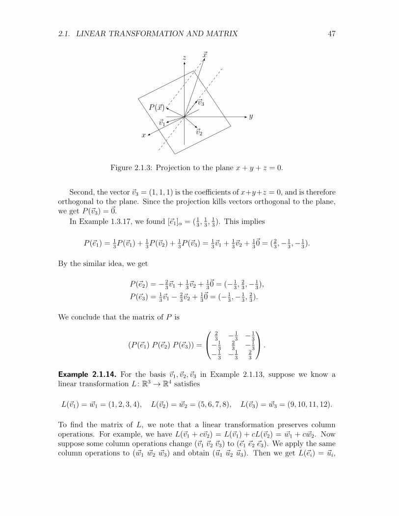
2.1. LINEAR TRANSFORMATION AND MATRIX 47
x
y
z
~v3
~v1
~v2
~x
P (~x)
Figure 2.1.3: Projection to the plane x+ y + z = 0.
Second, the vector ~v3 = (1, 1, 1) is the coefficients of x+y+z = 0, and is thereforeorthogonal to the plane. Since the projection kills vectors orthogonal to the plane,we get P (~v3) = ~0.
In Example 1.3.17, we found [~e1]α = (13, 1
3, 1
3). This implies
P (~e1) = 13P (~v1) + 1
3P (~v2) + 1
3P (~v3) = 1
3~v1 + 1
3~v2 + 1
3~0 = (2
3,−1
3,−1
3).
By the similar idea, we get
P (~e2) = −23~v1 + 1
3~v2 + 1
3~0 = (−1
3, 2
3,−1
3),
P (~e3) = 13~v1 − 2
3~v2 + 1
3~0 = (−1
3,−1
3, 2
3).
We conclude that the matrix of P is
(P (~e1) P (~e2) P (~e3)) =
23−1
3−1
3
−13
23−1
3
−13−1
323
.
Example 2.1.14. For the basis ~v1, ~v2, ~v3 in Example 2.1.13, suppose we know alinear transformation L : R3 → R4 satisfies
L(~v1) = ~w1 = (1, 2, 3, 4), L(~v2) = ~w2 = (5, 6, 7, 8), L(~v3) = ~w3 = (9, 10, 11, 12).
To find the matrix of L, we note that a linear transformation preserves columnoperations. For example, we have L(~v1 + c~v2) = L(~v1) + cL(~v2) = ~w1 + c~w2. Nowsuppose some column operations change (~v1 ~v2 ~v3) to (~e1 ~e2 ~e3). We apply the samecolumn operations to (~w1 ~w2 ~w3) and obtain (~u1 ~u2 ~u3). Then we get L(~ei) = ~ui,
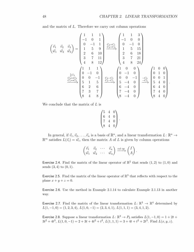
48 CHAPTER 2. LINEAR TRANSFORMATION
and the matrix of L. Therefore we carry out column operations
(~v1 ~v2 ~v3
~w1 ~w2 ~w3
)=
1 1 1−1 0 10 −1 11 5 92 6 103 7 114 8 12
C3+C1C3+C2−−−−→
1 1 3−1 0 00 −1 01 5 152 6 183 7 214 8 24
13C3
C2↔C3C1↔C2−−−−→
1 1 10 −1 00 0 −15 1 56 2 67 3 78 4 8
C2−C1C3−C1−−−−→
1 0 00 −1 00 0 −15 −4 06 −4 07 −4 08 −4 0
−C2−C3−−→
1 0 00 1 00 0 15 4 06 4 07 4 08 4 0
.
We conclude that the matrix of L is5 4 06 4 07 4 08 4 0
.
In general, if ~v1, ~v2, . . . , ~vn is a basis of Rn, and a linear transformation L : Rn →Rm satisfies L(~vi) = ~wi, then the matrix A of L is given by column operations(
~v1 ~v2 · · · ~vn~w1 ~w2 · · · ~wn
)col op−−−→
(IA
).
Exercise 2.4. Find the matrix of the linear operator of R2 that sends (1, 2) to (1, 0) andsends (3, 4) to (0, 1).
Exercise 2.5. Find the matrix of the linear operator of R3 that reflects with respect to theplane x+ y + z = 0.
Exercise 2.6. Use the method in Example 2.1.14 to calculate Example 2.1.13 in anotherway.
Exercise 2.7. Find the matrix of the linear transformation L : R3 → R4 determined byL(1,−1, 0) = (1, 2, 3, 4), L(1, 0,−1) = (2, 3, 4, 1), L(1, 1, 1) = (3, 4, 1, 2).
Exercise 2.8. Suppose a linear transformation L : R3 → P3 satisfies L(1,−1, 0) = 1 + 2t+3t2 + 4t3, L(1, 0,−1) = 2 + 3t+ 4t2 + t3, L(1, 1, 1) = 3 + 4t+ t2 + 2t3. Find L(x, y, z).

2.1. LINEAR TRANSFORMATION AND MATRIX 49
2.1.3 Operation of Linear Transformation
The addition of two linear transformations L,K : V → W is
(L+K)(~v) = L(~v) +K(~v) : V → W.
The following shows that L+K preserves the addition
(L+K)(~u+ ~v) = L(~u+ ~v) +K(~u+ ~v) (definition of L+K)
= (L(~u) + L(~v)) + (K(~u) +K(~v)) (L and K preserve addition)
= L(~u) +K(~u) + L(~v) +K(~v) (Axioms 1 and 2)
= (L+K)(~u) + (L+K)(~v). (definition of L+K)
We can similarly verify (L+K)(c~u) = c(L+K)(~u).The scalar multiplication of a linear transformation is
(cL)(~v) = cL(~v) : V → W.
We can similarly show that cL is a linear transformation.
Proposition 2.1.5. Hom(V,W ) is a vector space.
Proof. The following proves L+K = K + L
(L+K)(~u) = L(~u) +K(~u) = K(~u) + L(~u) = (K + L)(~u).
The first and third equalities are due to the definition of addition in Hom(V,W ).The second equality is due to Axiom 1 of vector space.
We can similarly prove the associativity (L + K) + M = L + (K + M). Thezero vector in Hom(V,W ) is the zero transformation O(~v) = ~0 in Example 2.1.1.The negative of L ∈ Hom(V,W ) is K(~v) = −L(~v). The other axioms can also beverified, and are left as exercises.
We can compose linear transformations K : U → V and L : V → W with match-ing domain and range
(L ◦K)(~v) = L(K(~v)) : U → W.
The composition preserves the addition
(L ◦K)(~u+ ~v) = L(K(~u+ ~v)) = L(K(~u) +K(~v))
= L(K(~u)) + L(K(~v)) = (L ◦K)(~u) + (L ◦K)(~v).
The first and fourth equalities are due to the definition of composition. The secondand third equalities are due to the linearity of L and K. We can similarly verifythat the composition preserves the scalar multiplication. Therefore the compositionis a linear transformation.

50 CHAPTER 2. LINEAR TRANSFORMATION
Example 2.1.15. The composition of two rotations is still a rotation: Rθ1 ◦ Rθ2 =Rθ1+θ2 .
Example 2.1.16. Consider the differential equation
(1 + t2)f ′′ + (1 + t)f ′ − f = t+ 2t3.
The left is the addition of three transformations f 7→ (1 + t2)f ′′, f 7→ (1 + t)f ′,f 7→ −f .
Let D(f) = f ′ be the derivative linear transformation in Example 2.1.6. LetMa(f) = af be the linear transformation of multiplying a function a(t). Then(1 + t2)f ′′ is the composition D2 = M1+t2 ◦ D ◦ D, (1 + t)f ′ is the compositionM1+t ◦D, and f 7→ −f is the linear transformation M−1. Therefore the left side ofthe differential equation is the linear transformation
L = M1+t2 ◦D ◦D +M1+t ◦D +M−1.
The differential equation can be expressed as L(f(t)) = b(t) with b(t) = t+2t3 ∈ C∞.In general, a linear differential equation of order n is
a0(t)dnf
dtn+ a1(t)
dn−1f
dtn−1+ a2(t)
dn−2f
dtn−2+ · · ·+ an−1(t)
df
dt+ an(t)f = b(t).
If the coefficient functions a0(t), a1(t), . . . , an(t) are smooth, then the left side is alinear transformation C∞ → C∞.
Exercise 2.9. Interpret the Newton-Leibniz formula f(t) = f(0)+∫ t
0 f′(τ)dτ as an equality
of linear transformations.
Exercise 2.10. The trace of a square matrix A = (aij) is the sum of its diagonal entries
trA = a11 + a22 + · · ·+ ann.
Explain that the trace is a linear functional on the vector space of Mn×n of n×n matrices,and trAT = trA.
Exercise 2.11. Fix a vector ~v ∈ V . Prove that the evaluation map L 7→ L(~v) : Hom(V,W )→W is a linear transformation.
Exercise 2.12. Let L : V →W be a linear transformation.
1. Prove that L ◦ (K1 +K2) = L ◦K1 + L ◦K2 and L ◦ (aK) = a(L ◦K).
2. Explain that the first part means that the map L∗ = L◦· : Hom(U, V )→ Hom(U,W )is a linear transformation.
3. Prove that I∗ = I, (L+K)∗ = L∗ +K∗, (aL)∗ = aL∗ and (L ◦K)∗ = L∗ ◦K∗.

2.1. LINEAR TRANSFORMATION AND MATRIX 51
4. Prove that L 7→ L∗ : Hom(V,W )→ Hom(Hom(U, V ), Hom(U,W )) is a linear trans-formation.
Exercise 2.13. Let L : V →W be a linear transformation.
1. Prove that (K1 +K2) ◦ L = K1 ◦ L+K2 ◦ L and (aK) ◦ L = a(K ◦ L).
2. Prove that L∗ = · ◦ L : Hom(W,U)→ Hom(V,U) is a linear transformation.
3. Prove that I∗ = I, (L+K)∗ = L∗ +K∗, (aL)∗ = aL∗ and (L ◦K)∗ = K∗ ◦ L∗.
4. Prove that L 7→ L∗ : Hom(V,W )→ Hom(Hom(W,U), Hom(V,U)) is a linear trans-formation.
Exercise 2.14. Denote by Map(X,Y ) all the maps from a set X to another set Y . For amap f : X → Y and any set Z, define
f∗ = f◦ : Map(Z,X)→ Map(Z, Y ), f∗ = ◦f : Map(Y,Z)→ Map(X,Z).
Prove that (f ◦ g)∗ = f∗ ◦ g∗ and (f ◦ g)∗ = g∗ ◦ f∗. This shows that (L ◦K)∗ = L∗ ◦K∗ inExercise 2.12 and (L◦K)∗ = K∗◦L∗ in Exercise 2.13 do not require linear transformation.
2.1.4 Matrix Operation
In Section 2.1.2, we have the equivalence
L ∈ Hom(Rn,Rm)←→ A ∈Mm×n, L(~x) = A~x, A = (L(~e1) L(~e2) · · · L(~en)).
Any operation we can do on one side should be reflected on the other side. Forexample, we know Hom(Rn,Rm) is a vector space. We define the addition andscalar multiplication of matrices in Mm×n in such a way to make the invertible mapHom(Rn,Rm)←→Mm×n an isomorphism of vector spaces.
Let L,K : Rn → Rm be linear transformations, with respective matrices
A =
a11 a12 . . . a1n
a21 a22 . . . a2n...
......
am1 am2 . . . amn
, B =
b11 b12 . . . b1n
b21 b22 . . . b2n...
......
bm1 bm2 . . . bmn
.
Then the i-th column of the matrix of L+K : Rn → Rm is
(L+K)(~ei) = L(~ei) +K(~ei) =
a1i
a2i...ami
+
b1i
b2i...bmi
=
a1i + b1i
a2i + b2i...
ami + bmi
.
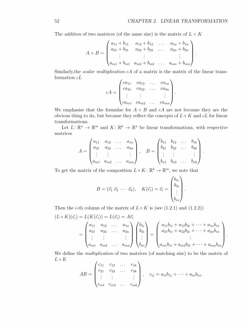
52 CHAPTER 2. LINEAR TRANSFORMATION
The addition of two matrices (of the same size) is the matrix of L+K
A+B =
a11 + b11 a12 + b12 . . . a1n + b1n
a21 + b21 a22 + b22 . . . a2n + b2n...
......
am1 + bm1 am2 + bm2 . . . amn + bmn
.
Similarly,the scalar multiplication cA of a matrix is the matrix of the linear trans-formation cL
cA =
ca11 ca12 . . . ca1n
ca21 ca22 . . . ca2n...
......
cam1 cam2 . . . camn
.
We emphasise that the formulae for A + B and cA are not because they are theobvious thing to do, but because they reflect the concepts of L+K and cL for lineartransformations.
Let L : Rn → Rm and K : Rk → Rn be linear transformations, with respectivematrices
A =
a11 a12 . . . a1n
a21 a22 . . . a2n...
......
am1 am2 . . . amn
, B =
b11 b12 . . . b1k
b21 b22 . . . b2k...
......
bn1 bn2 . . . bnk
.
To get the matrix of the composition L ◦K : Rk → Rm, we note that
B = (~v1 ~v2 · · · ~vk), K(~ei) = ~vi =
b1i
b2i...bni
.
Then the i-th column of the matrix of L ◦K is (see (1.2.1) and (1.2.2))
(L ◦K)(~ei) = L(K(~ei)) = L(~vi) = A~vi
=
a11 a12 . . . a1n
a21 a22 . . . a2n...
......
am1 am2 . . . amn
b1i
b2i...bni
=
a11b1i + a12b2i + · · ·+ a1nbnia21b1i + a22b2i + · · ·+ a2nbni
...am1b1i + am2b2i + · · ·+ amnbni
.
We define the multiplication of two matrices (of matching size) to be the matrix ofL ◦K
AB =
c11 c12 . . . c1k
c21 c22 . . . c2k...
......
cm1 cm2 . . . cmk
, cij = ai1b1j + · · ·+ ainbnj.
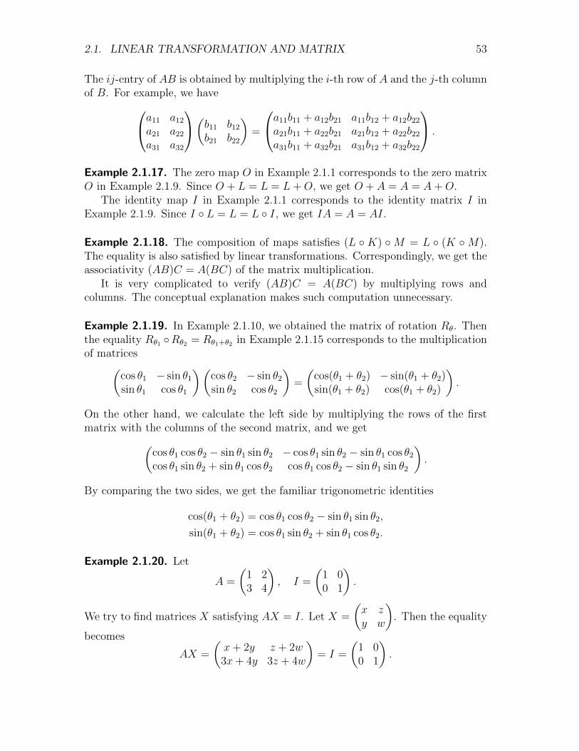
2.1. LINEAR TRANSFORMATION AND MATRIX 53
The ij-entry of AB is obtained by multiplying the i-th row of A and the j-th columnof B. For example, we havea11 a12
a21 a22
a31 a32
(b11 b12
b21 b22
)=
a11b11 + a12b21 a11b12 + a12b22
a21b11 + a22b21 a21b12 + a22b22
a31b11 + a32b21 a31b12 + a32b22
.
Example 2.1.17. The zero map O in Example 2.1.1 corresponds to the zero matrixO in Example 2.1.9. Since O + L = L = L+O, we get O + A = A = A+O.
The identity map I in Example 2.1.1 corresponds to the identity matrix I inExample 2.1.9. Since I ◦ L = L = L ◦ I, we get IA = A = AI.
Example 2.1.18. The composition of maps satisfies (L ◦ K) ◦M = L ◦ (K ◦M).The equality is also satisfied by linear transformations. Correspondingly, we get theassociativity (AB)C = A(BC) of the matrix multiplication.
It is very complicated to verify (AB)C = A(BC) by multiplying rows andcolumns. The conceptual explanation makes such computation unnecessary.
Example 2.1.19. In Example 2.1.10, we obtained the matrix of rotation Rθ. Thenthe equality Rθ1 ◦Rθ2 = Rθ1+θ2 in Example 2.1.15 corresponds to the multiplicationof matrices(
cos θ1 − sin θ1
sin θ1 cos θ1
)(cos θ2 − sin θ2
sin θ2 cos θ2
)=
(cos(θ1 + θ2) − sin(θ1 + θ2)sin(θ1 + θ2) cos(θ1 + θ2)
).
On the other hand, we calculate the left side by multiplying the rows of the firstmatrix with the columns of the second matrix, and we get(
cos θ1 cos θ2 − sin θ1 sin θ2 − cos θ1 sin θ2 − sin θ1 cos θ2
cos θ1 sin θ2 + sin θ1 cos θ2 cos θ1 cos θ2 − sin θ1 sin θ2
).
By comparing the two sides, we get the familiar trigonometric identities
cos(θ1 + θ2) = cos θ1 cos θ2 − sin θ1 sin θ2,
sin(θ1 + θ2) = cos θ1 sin θ2 + sin θ1 cos θ2.
Example 2.1.20. Let
A =
(1 23 4
), I =
(1 00 1
).
We try to find matrices X satisfying AX = I. Let X =
(x zy w
). Then the equality
becomes
AX =
(x+ 2y z + 2w3x+ 4y 3z + 4w
)= I =
(1 00 1
).

54 CHAPTER 2. LINEAR TRANSFORMATION
This means two systems of linear equations
x + 2y = 1,
3x + 4y = 0;
z + 2w = 0,
3z + 4w = 1.
We can solve two systems simultaneously by the row operations
(A I) =
(1 2 1 03 4 0 1
)→(
1 2 1 00 −2 −3 1
)→(
1 0 −2 10 1 3
2−1
2
).
From the first three columns, we get x = −2 and y = 32. from the first, second and
fourth columns, we get z = 1 and w = −12. Therefore
X =
(−2 1
32−1
2
).
In general, to solve AX = B, we may carry out the row operation on the matrix(A B).
Exercise 2.15. Composing the reflection Fρ in Examples 2.1.3 and 2.1.10 with itself is theidentity. Explain that this means the trigonometric identity cos2 θ + sin2 θ = 1.
Exercise 2.16. Geometrically, one can see the following compositions of rotations andrefelctions.
1. Rθ ◦ Fρ is a reflection. What is the angle of reflection?
2. Fρ ◦Rθ is a reflection. What is the angle of reflection?
3. Fρ1 ◦ Fρ2 is a rotation. What is the angle of rotation?
Interpret the geometrical observations as trigonometric identities.
Exercise 2.17. Use some examples (say rotations and reflections) to show that for two n×nmatrices, AB may not be equal to BA.
Exercise 2.18. Use the formula for matrix addition to show the commutativity A + B =B+A and the associativity (A+B)+C = A+(B+C). Then give a conceptual explanationto the properties without using calculation.
Exercise 2.19. Explain that the addition and scalar multiplication of matrices make the setMm×n of m×n matrices into a vector space. Moreover, the matrix of linear transformationgives an isomorphism (i.e., invertible linear transformation) Hom(Rn,Rm)→Mm×n.
Exercise 2.20. Explain that Exercise 2.12 means that the matrix multiplication satisfiesA(B + C) = AB + AC, A(aB) = a(AB), and the left multiplication X 7→ AX is a lineartransformation.

2.1. LINEAR TRANSFORMATION AND MATRIX 55
Exercise 2.21. Explain that Exercise 2.13 means that the matrix multiplication satisfies(A+B)C = AC+BC, (aA)B = a(AB), and the right multiplication X 7→ XA is a lineartransformation.
Exercise 2.22. Let A be an m × n matrix and let B be a k × m matrix. For the tracedefined in Example 2.10, explain that trAXB is a linear functional for X ∈Mn×k.
Exercise 2.23. Let A be an m × n matrix and let B be an n ×m matrix. Prove that thetrace defined in Example 2.10 satisfies trAB = trBA.
Exercise 2.24. Add or multiply matrices, whenever you can.
1.
(1 23 4
).
2.
(4 −2−3 1
).
3.
(0 1 01 0 1
).
4.
(1 0 10 1 0
).
5.
0 11 00 1
.
6.
1 1 11 1 11 1 1
.
Exercise 2.25. Find the n-th power matrix An (i.e., multiply the matrix to itself n times).
1.
(cos θ − sin θsin θ cos θ
).
2.
(cos θ sin θsin θ − cos θ
).
3.
a1 0 0 00 a2 0 00 0 a3 00 0 0 a4
.
4.
0 a 0 00 0 a 00 0 0 a0 0 0 0
.
5.
a b 0 00 a b 00 0 a b0 0 0 a
.
Exercise 2.26. Solve the matrix equations.
1.
(1 2 34 5 6
)X =
(7 89 10
).
2.
1 42 53 6
X =
7 108 11a b
.
3.
1 25 69 10
X =
3 47 811 b
.
Exercise 2.27. For the transpose of 2×2 matrices, verify that (AB)T = BTAT (the concep-tual reason will be given in Section 2.4.2).) Then use this to solve the matrix equations.
1. X
(1 23 4
)=
(1 00 1
). 2.
(1 23 4
)X
(4 −3−2 1
)=
(1 00 1
).

56 CHAPTER 2. LINEAR TRANSFORMATION
Exercise 2.28. Let A =
(−1 00 1
). Find all the matrices X satisfying AX = XA. Gener-
alise your result to diagonal matrix
A =
a1 0 · · · 00 a2 · · · 0...
......
0 0 · · · an
.
2.1.5 Elementary Matrix and LU-Decomposition
The row operations can be interpreted as multiplying on the left by some specialmatrices, called elementary matrices. In fact, the special matrix is obtained by ap-plying the same row operation to the identity matrix I. For example, by exchangingthe 2nd and 4th rows, by multiplying c to the 2nd row, and by adding c multiplesof the 3rd row to the 1st row, we get respectively
T24 =
1 0 0 00 0 0 10 0 1 00 1 0 0
, D2(c) =
1 0 0 00 c 0 00 0 1 00 0 0 1
, E13(c) =
1 0 c 00 1 0 00 0 1 00 0 0 1
.
Then
1. TijA exchanges i-th and j-th rows of A.
2. Di(c)A multiplies c to the i-th row of A.
3. Eij(c)A adds the c multiple of the j-th row to the i-th row.
Note that the elementary matrices can also be obtained by applying similarcolumn operations (already appeared in Exercises 1.32, 1.37, 1.59) to I. Then wehave
1. ATij exchanges i-th and j-th columns of A.
2. ADi(a) multiplies a to the i-th column of A.
3. AEij(a) adds the a multiple of the i-th column to the j-th column.
We know that any matrix can become (reduced) row echelon form after some rowoperations. This means that multiplying the left of the matrix by some elementarymatrices gives a (reduced) row echelon form.
Example 2.1.21. We have
T24D2(c) =
1 0 0 00 0 0 10 0 1 00 2 0 0
= D4(c)T24.

2.1. LINEAR TRANSFORMATION AND MATRIX 57
The equality can be obtained in four ways:
1. T24×: Exchange the 2nd and 4th rows of D2(c).
2. ×D2(c): Multiplying c to the 2nd column of T24.
3. ×T24: Exchange the 2nd and 4th columns of D4(c).
4. D4(c)×: Multiplying c to the 4th row of T24.
In general, we get TijDi(c) = Dj(c)Tij. We also have TijDj(c) = Di(c)Tij. Moreover,we have TijDk(c) = Dk(c)Tij for distinct i, j, k.
Example 2.1.22. The row operations in Example 1.2.1 can be interpreted as1 0 00 −1
30
0 0 1
1 0 00 1 00 −2 1
1 0 00 1 0−3 0 1
1 0 0−2 1 00 0 1
1 4 7 102 5 8 113 6 9 12
=
1 4 7 100 1 2 30 0 0 0
= U.
Here U is an upper triangle matrix. On the other hand, we used row operations cRi
and Ri + cRj with j < i. This means that all the elementary matrices are lowertriangular. The we move the elementary matrices to the right, and use Di(c)
−1 =Di(c
−1) and Eij(c)−1 = Eij(−c) to get1 4 7 10
2 5 8 113 6 9 12
=
1 0 02 1 00 0 1
1 0 00 1 03 0 1
1 0 00 1 00 2 1
1 0 00 −3 00 0 1
1 4 7 100 1 2 30 0 0 0
=
1 0 02 −3 03 −6 1
1 4 7 100 1 2 30 0 0 0
= LU.
We may also move −3 to U (i.e., remove D2(−13)) and get1 4 7 10
2 5 8 113 6 9 12
=
1 0 02 1 03 2 1
1 4 7 100 −3 −6 −90 0 0 0
.
The example shows that, if we can use only Ri + cRj with j < i to get a rowechelon form U of A, then we can write A = LU , where L is the combination of

58 CHAPTER 2. LINEAR TRANSFORMATION
the inverse of these Ri + cRj, and is a lower triangular square matrix with nonzerodiagonals. This is the LU-decomposition of the matrix A.
Not every matrix has LU -decomposition. For example, if a11 = 0 in A, then weneed to first exchange rows to make the term nonzero
A =
0 1 2 31 2 3 42 3 4 5
R1↔R2−−−−→
1 2 3 40 1 2 32 3 4 5
R3−2R1R3+R2−−−−→
1 2 3 40 1 2 30 0 0 0
= U.
This gives
PA =
0 1 01 0 00 0 1
0 1 2 31 2 3 42 3 4 5
=
1 0 00 1 02 −1 1
1 2 3 40 1 2 30 0 0 0
= LU.
Here the left multiplication by P permutes rows. In general, every matrix has LU -decomposition after suitable permutation of rows.
The LU -decomposition is useful for solving A~x = ~b. We may first solve L~y = ~bto get ~y and then solve U~x = ~y. Since L is lower triangular, it is easy to get theunique solution ~y by forward substitution. Since U is upper triangular, we can usebackward substituting to solve U~x = ~y.
Exercise 2.29. Write down the 5× 5 matrices: T24, T42, D4(c), E35(c), E53(c).
Exercise 2.30. What do you get by multiplying T13E13(−2)D2(3) to the left of1 4 72 5 83 6 9
.
What about multiplying on the right?
Exercise 2.31. Explain the following equalities
T 2ij = I,
Di(a)Di(b) = Di(ab),
Eij(a)Eij(b) = Eij(a+ b),
Eij(a) = Eik(a)Ekj(1)Eik(a)−1Ekj(1)−1.
Can you come up with some other equalities?
Exercise 2.32. Find the LU -decompositions of the matrices in Exercise 1.28 that do notinvolve parameters.
Exercise 2.33. The LU -decompositions is derived from using row operations of third type(and maybe also second type) to get a row echelon form. What do you get by using thesimilar column operations.

2.2. ONTO, ONE-TO-ONE, AND INVERSE 59
2.2 Onto, One-to-one, and Inverse
Definition 2.2.1. Let f : X → Y be a map.
1. f is onto (or surjective) if for any y ∈ Y , there is x ∈ X, such that f(x) = y.
2. f is one-to-one (or injective) if f(x) = f(x′) implies x = x′.
3. f is a one-to-one correspondence (or bijective) if it is onto and one-to-one.
The onto property can be regarded as that the equation f(x) = y has solutionfor all the right side y.
The one-to-one property also means that x 6= x′ implies f(x) 6= f(x′). Theproperty can be regarded as that uniqueness of the solution of the equation f(x) = y.
Proposition 2.2.2. Let f : X → Y be a map.
1. f is onto if and only if f has right inverse: There is a map g : Y → X, suchthat f ◦ g = idY .
2. f is one-to-one if and only if f has left inverse: There is a map g : Y → X,such that g ◦ f = idX .
3. f is a one-to-one correspondence if and only if it has inverse: There is a mapg : Y → X, such that f ◦ g = idY and g ◦ f = idX .
In the third statement, the map f is invertible, with inverse map g denotedg = f−1.
Proof. If f ◦ g = idY , then for any y ∈ Y , we have f(g(y)) = y. In other words,x = g(y) satisfies f(x) = y. Conversely, suppose f : X → Y is onto. We constructa map g : Y → X as follows. For any y ∈ Y , by f onto, we can find some x ∈ Xsatisfying f(x) = y. We choose one such x (strictly speaking, this uses the Axiomof Choice) and define g(y) = x. Then the map g satisfies (f ◦ g)(y) = f(x) = y.
If g ◦ f = idX , then we have g(f(x)) = x. Therefore
f(x) = f(x′) =⇒ g(f(x)) = g(f(x′)) =⇒ x = x′.
Conversely, suppose f : X → Y is one-to-one. We fix an element x0 ∈ X andconstruct a map g : Y → X as follows. For any y ∈ Y , if y = f(x) for some x ∈ X(i.e., y lies in the image of f), then we define g(y) = x. If we cannot find such x,then we define g(y) = x0. Note that in the first case, if y = f(x′) for another x′ ∈ X,then by f one-to-one, we have x′ = x. This shows that g is well defined. For thecase y = f(x), our construction of g implies (g ◦ f)(x) = g(f(x)) = x.
From the first and second parts, we know a map f is onto and one-to-one if andonly if there are maps g and h, such that f ◦ g = id and h ◦ f = id. Compared with

60 CHAPTER 2. LINEAR TRANSFORMATION
the definition of invertibility, for the third statement, we only need to show g = h.This follows from g = id ◦ g = h ◦ f ◦ g = h ◦ id = h.
Example 2.2.1. Consider the map (f =) Instructor: Courses → Professors.
The map is onto means every professor teaches some course. The map g inProposition 2.2.2 can take a professor (say me) to any one course (say linear algebra)the professor teaches.
The map is one-to-one means any professor either teaches one course, or does notteach any course. This also means that no professor teaches two or more courses.If a professor (say me) teaches one course, then the map g in Proposition 2.2.2takes the professor to the unique course (say linear algebra) the professor teaches.If a professor does not teach any course, then g may take the professor to any oneexisting course.
Example 2.2.2. The identity map I(x) = x : X → X is always onto and one-to-one,with I−1 = I.
The zero map O(~v) = ~0: V → W in Example 2.1.1 is onto if and only if W isthe zero vector space in Example 1.1.1. The zero map is one-to-one if and only if Vis the zero vector space.
The coordinate map in Section 1.3.7 is onto and one-to-one, with the linearcombination map as the inverse.
The rotation and flipping in Example 2.1.3 are invertible, with R−1θ = R−θ and
F−1θ = Fθ.
Exercise 2.34. Prove that the composition of onto maps is onto.
Exercise 2.35. Prove that the composition of one-to-one maps is one-to-one.
Exercise 2.36. Prove that the composition of invertible maps is invertible. Moreover, wehave (f ◦ g)−1 = g−1 ◦ f−1.
Exercise 2.37. Prove that if f ◦ g is onto, then f is onto. Prove that if g ◦ f is one-to-one,then f is one-to-one.
2.2.1 Onto and One-to-one for Linear Transformation
For a linear transformation L : V → W , we may regard the onto and one-to-oneproperties as the existence and uniqueness of solutions of the equation L(~x) = ~b. Forthe case V and W are Euclidean spaces, this becomes the existence and uniquenessof solutions of the system of linear equations A~x = ~b. This can be determined bythe row echelon form of the matrix A.
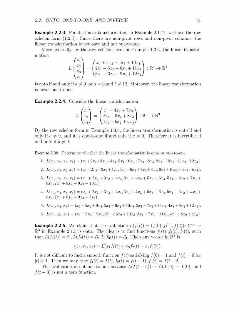
2.2. ONTO, ONE-TO-ONE, AND INVERSE 61
Example 2.2.3. For the linear transformation in Example 2.1.12, we have the rowechelon form (1.2.3). Since there are non-pivot rows and non-pivot columns, thelinear transformation is not onto and not one-to-one.
More generally, by the row echelon form in Example 1.3.6, the linear transfor-mation
L
x1
x2
x3
x4
=
x1 + 4x2 + 7x3 + 10x4
2x1 + 5x2 + 8x3 + 11x4
3x1 + 6x2 + 9x3 + 12x4
: R4 → R3
is onto if and only if a 6= 9, or a = 0 and b 6= 12. Moreover, the linear transformationis never one-to-one.
Example 2.2.4. Consider the linear transformation
L
x1
x2
x3
=
x1 + 4x2 + 7x3
2x1 + 5x2 + 8x3
3x1 + 6x2 + ax3
: R3 → R3
By the row echelon form in Example 1.3.6, the linear transformation is onto if andonly if a 6= 9, and it is one-to-one if and only if a 6= 9. Therefore it is invertible ifand only if a 6= 9.
Exercise 2.38. Determine whether the linear transformation is onto or one-to-one.
1. L(x1, x2, x3, x4) = (x1+2x2+3x3+4x4, 5x1+6x2+7x3+8x4, 9x1+10x2+11x3+12x4).
2. L(x1, x2, x3, x4) = (x1+2x2+3x3+4x4, 5x1+6x2+7x3+8x4, 9x1+10x2+ax3+bx4).
3. L(x1, x2, x3, x4) = (x1 + 2x2 + 3x3 + 4x4, 3x1 + 4x2 + 5x3 + 6x4, 5x1 + 6x2 + 7x3 +8x4, 7x1 + 8x2 + 9x3 + 10x4)
4. L(x1, x2, x3, x4) = (x1 + 2x2 + 3x3 + 4x4, 3x1 + 4x2 + 5x3 + 6x4, 5x1 + 6x2 + ax3 +8x4, 7x1 + 8x2 + 9x3 + bx4).
5. L(x1, x2, x3) = (x1 +5x2 +9x3, 2x1 +6x2 +10x3, 3x1 +7x2 +11x3, 4x1 +8x2 +12x3).
6. L(x1, x2, x3) = (x1 + 5x2 + 9x3, 2x1 + 6x2 + 10x3, 3x1 + 7x2 + 11x3, 4x1 + 8x2 +ax3).
Example 2.2.5. We claim that the evaluation L(f(t)) = (f(0), f(1), f(2)) : C∞ →R3 in Example 2.1.5 is onto. The idea is to find functions f1(t), f2(t), f3(t), suchthat L(f1(t)) = ~e1, L(f2(t)) = ~e2, L(f3(t)) = ~e3. Then any vector in R3 is
(x1, x2, x3) = L(x1f1(t) + x3f2(t) + x3f3(t)).
It is not difficult to find a smooth function f(t) satisfying f(0) = 1 and f(t) = 0 for|t| ≥ 1. Then we may take f1(t) = f(t), f2(t) = f(t− 1), f3(t) = f(t− 2).
The evaluation is not one-to-one because L(f(t − 3)) = (0, 0, 0) = L(0), andf(t− 3) is not a zero function.

62 CHAPTER 2. LINEAR TRANSFORMATION
Example 2.2.6. The derivation operator in Example 2.1.6 is onto due to the Newton-Leibniz formula. For any g ∈ C∞, we have g = f ′ for f(t) =
∫ t0g(τ)dτ ∈ C∞. It is
not one-to-one because all the constant functions are mapped to the zero function.The integration operator in Example 2.1.6 is not onto because any function
g(t) =∫ t
0f(τ)dτ must satisfy g(0) = 0. The operator is one-to-one because taking
derivative of∫ t
0f1(τ)dτ =
∫ t0f2(τ)dτ implies f1(t) = f2(t).
In fact, the Newton-Leibniz formula says derivation ◦ integration is the identitymap. Then by Proposition 2.2.2, the derivation is onto and the integration is one-to-one.
need exercises
Proposition 2.2.3. Suppose L : V → W is a linear transformation, and V,W arefinite dimensional. The following are equivalent.
1. L is onto.
2. L takes a spanning set of V to a spanning set of W .
3. There is a linear transformation K : W → V satisfying L ◦K = IW .
From the proof below, we note that the equivalence of the first two statementsonly needs V to be finite dimensional, and the equivalence of the first and thirdstatements only needs W to be finite dimensional.
Proof. Suppose ~v1, ~v2, . . . , ~vn span V . Then
~x ∈ V =⇒ ~x = x1~v1 + x2~v2 + · · ·+ xn~vn
=⇒ L(~x) = x1L(~v1) + x2L(~v2) + · · ·+ xnL(~vn).
The equality shows the first two statements are equivalent
L is onto ⇐⇒ L(~x) can be all the vectors in W
⇐⇒ L(~v1), L(~v2), . . . , L(~vn) span W.
By Proposition 2.2.2, we know the third statement implies the first. Conversely,assume L is onto. For a basis ~w1, ~w2, . . . , ~wm of W , we can find ~vi ∈ V satisfyingL(~vi) = ~wi. By Proposition 2.1.4, there is a linear transformation K : W → Vsatisfying K(~wi) = ~vi. By (L ◦K)(~wi) = L(K(~wi)) = L(~vi) = ~wi and Proposition2.1.2, we get L ◦K = IW .
Proposition 2.2.4. Suppose L : V → W is a linear transformation, and W is finitedimensional. The following are equivalent.
1. L is one-to-one.

2.2. ONTO, ONE-TO-ONE, AND INVERSE 63
2. L takes a linearly independent set in V to a linearly independent set in W .
3. L(~v) = ~0 implies ~v = ~0.
4. There is a linear transformation K : W → V satisfying K ◦ L = IV .
From the proof below, we note that the equivalence of the first three statementsdoes not need W to be finite dimensional.
Proof. Suppose L is one-to-one and vectors ~v1, ~v2, . . . , ~vn in V are linearly indepen-dent. The following shows that L(~v1), L(~v2), . . . , L(~vn) are linearly independent
x1L(~v1) + x2L(~v2) + · · ·+ xnL(~vn) = y1L(~v1) + y2L(~v2) + · · ·+ ynL(~vn)
=⇒ L(x1~v1 + x2~v2 + · · ·+ xn~vn) = L(y1~v1 + y2~v2 + · · ·+ yn~vn) (L is linear)
=⇒ x1~v1 + x2~v2 + · · ·+ xn~vn = y1~v1 + y2~v2 + · · ·+ yn~vn (L is one-to-one)
=⇒ x1 = y1, x2 = y2, . . . , xn = yn. (~v1, ~v2, . . . , ~vn are linearly independent)
Next we assume the second statement. If ~v 6= ~0, then by Example 1.3.10, thesingle vector ~v is linearly independent. By the assumption, the single vector L(~v)is also linearly independent. Again by Example 1.3.10, this means L(~v) 6= ~0. Thisproves ~v 6= ~0 =⇒ L(~v) 6= ~0, which is the same as L(~v) = ~0 =⇒ ~v = ~0.
The following proves that the third statement implies the first
L(~x) = L(~y) =⇒ L(~x− ~y) = L(~x)− L(~y) = ~0 =⇒ ~x− ~y = ~0 =⇒ ~x = ~y.
This completes the proof that the first three statements are equivalent.By Proposition 2.2.2, we know the fourth statement implies the first. It remains
to prove that the first three statements imply the fourth. This makes use of theassumption that W is finite dimensional.
Suppose ~v1, ~v2, . . . , ~vn in V are linearly independent. By the second statement,the vectors ~w1 = L(~v1), ~w2 = L(~v2), . . . , ~wn = L(~vn) in W are also linearly indepen-dent. By Proposition 1.3.13, we get n ≤ dimW . Since dimW is finite, this impliesthat V is also finite dimensional. Therefore V has a basis, which we still denoteby {~v1, ~v2, . . . , ~vn}. By Theorem 1.3.11, the corresponding linearly independent set{~w1, ~w2, . . . , ~wn} can be extended to a basis {~w1, ~w2, . . . , ~wn, ~wn+1, . . . , ~wm} ofW . ByProposition 2.1.4, there is a linear transformation K : W → V satisfying K(~wi) = ~vifor i ≤ n and K(~wi) = ~0 for n < i ≤ m. By (K ◦ L)(~vi) = K(L(~vi)) = K(~wi) = ~vifor i ≤ n and Proposition 2.1.2, we get K ◦ L = IV .
The following is comparable to Proposition 1.3.13. It reflects the intuition that, ifevery professor teaches some course (see Example 2.2.1), then the number of coursesis more than the number of professors. On the other hand, if each professor teachesat most one course, then the number of courses is less than the number of professors.

64 CHAPTER 2. LINEAR TRANSFORMATION
Proposition 2.2.5. Suppose L : V → W is a linear transformation between finitedimensional vector spaces.
1. If L is onto, then dimV ≥ dimW .
2. If L is one-to-one, then dimV ≤ dimW .
Proof. Suppose α = {~v1, ~v2, . . . , ~vn} is a basis of V . We denote the image of thebasis by L(α) = {L(~v1), L(~v2), . . . , L(~vn)}.
If L is onto, then by Proposition 2.2.3, L(α) spans W . By the first part of Propo-sition 1.3.13, we get dimV = n ≥ dimW . If L is one-to-one, then by Proposition2.2.4, L(α) is linearly independent. By the second part of Proposition 1.3.13, we getdimV = n ≤ dimW .
The following is the linear transformation version of Theorem 1.3.14.
Theorem 2.2.6. Suppose L : V → W is a linear transformation between finite di-mensional vector spaces. Then any two of the following imply the third.
• L is onto.
• L is one-to-one.
• dimV = dimW .
Let ~v1, ~v2, . . . , ~vn be a basis of V . The equivalence follows from Theorem 1.3.14,and applying the equivalence of the first two statements in Propositions 2.2.3 and2.2.4.
Example 2.2.7. For the evaluation L(f(t)) = (f(0), f(1), f(2)) : C∞ → R3 inExample 2.1.5, we find the functions f1(t), f2(t), f3(t) in Example 2.2.5 satisfy-ing L(f1(t)) = ~e1, L(f2(t)) = ~e2, L(f3(t)) = ~e3. This means that K(x1, x2, x3) =x1f1(t) + x3f2(t) + x3f3(t) satisfies L ◦K = I. This is actually the reason for L tobe onto in Example 2.2.5.
Example 2.2.8. The differential equation f ′′+(1+t2)f ′+tf = b(t) in Example 2.1.16can be interpreted as L(f(t)) = b(t) for a linear transformation L : C∞ → C∞. If weregard L as a linear transformation L : Pn → Pn+1 (restricting L to polynomials),then by Proposition 2.2.5, the restriction linear transformation is not onto. Forexample, we can find a polynomial b(t) of degree 5, such that f ′′+(1+t2)f ′+tf = b(t)cannot be solved for a polynomial f(t) of degree 4.
Exercise 2.39. Show that the linear combination map L(x1, x2, x3) = x1 cos t + x2 sin t +x3e
t : R3 → C∞ in Example 2.1.5 is not onto and is one-to-one.
2.2. ONTO, ONE-TO-ONE, AND INVERSE 65
Exercise 2.40. Show that the multiplication map f(t) 7→ a(t)f(t) : C∞ → C∞ in Example2.1.6 is onto if and only if a(t) 6= 0 everywhere. Show that the map is one-to-one if a(t) = 0at only finitely many places.
Exercise 2.41. Strictly speaking, the second statement of Proposition 2.2.3 can be aboutone spanning set or all spanning sets of V . Show that the two versions are equivalent.What about the second statement of Proposition 2.2.4?
Exercise 2.42. Suppose α is a basis of V . Prove that a linear transformation L : V → Wis onto if and only if L(α) spans W , and L is one-to-one if and only if L(α) is linearlyindependent.
Exercise 2.43. Prove that a linear transformation is onto if it takes a (not necessarilyspanning) set to a spanning set.
Exercise 2.44. Suppose L : V → W is an onto linear transformation. If V is finite dimen-sional, prove that W is finite dimensional.
Exercise 2.45. Let A be an m×n matrix. Explain that a system of linear equations A~x = ~bhas solution for all ~b ∈ Rm if and only if there is an n×m matrix B, such that AB = Im.Moreover, the solution is unique if and only if there is B, such that BA = In.
Exercise 2.46. Suppose L ◦K and K are linear transformations. Prove that if K is onto,then L is also a linear transformation.
Exercise 2.47. Suppose L ◦K and L are linear transformations. Prove that if L is one-to-one, then K is also a linear transformation.
Exercise 2.48. Recall the induced maps f∗ and f∗ in Exercise 2.14. Prove that if f is onto,then f∗ is onto and f∗ is one-to-one. Prove that if f is one-to-one, then f∗ is one-to-oneand f∗ is onto.
Exercise 2.49. Suppose L is an onto linear transformation. Prove that two linear transfor-mations K and K ′ are equal if and only if K ◦L = K ′ ◦L. What does this tell you aboutthe linear transformation L∗ : Hom(V,W )→ Hom(U,W ) in Exercise 2.13?
Exercise 2.50. Suppose L is a one-to-one linear transformation. Prove that two lineartransformations K and K ′ are equal if and only if L ◦K = L ◦K ′. What does this tellyou about the linear transformation L∗ : Hom(U, V )→ Hom(U,W ) in Exercise 2.12?
2.2.2 Isomorphism
Definition 2.2.7. An invertible linear transformation is an isomorphism. If thereis an isomorphism between two vector spaces V and W , then we say V and W are

66 CHAPTER 2. LINEAR TRANSFORMATION
isomorphic, and denote V ∼= W .
The isomorphism can be used to translate the linear algebra in one vector spaceto the linear algebra in another vector space.
Theorem 2.2.8. If a linear transformation L : V → W is an isomorphism, thenthe inverse map L−1 : W → V is also a linear transformation. Moreover, suppose~v1, ~v2, . . . , ~vn are vectors in V .
1. ~v1, ~v2, . . . , ~vn span V if and only if L(~v1), L(~v2), . . . , L(~vn) span W .
2. ~v1, ~v2, . . . , ~vn are linearly independent if and only if L(~v1), L(~v2), . . . , L(~vn) arelinearly independent.
3. ~v1, ~v2, . . . , ~vn form a basis of V if and only if L(~v1), L(~v2), . . . , L(~vn) form abasis of W .
The linearity of L−1 follows from Exercise 2.46 or 2.47. The rest of the proposi-tion follows from the second statements in Propositions 2.2.3 and 2.2.4.
Example 2.2.9. Given a basis α of V , we explained in Section 1.3.7 that the α-coordinate map [·]α : V → Rn has an inverse. Therefore the α-coordinate map is anisomorphism.
Example 2.2.10. A linear transformation L : R→ V gives a vector L(1) ∈ V . Thisis a linear map (see Exercise 2.11)
L ∈ Hom(R, V ) 7→ L(1) ∈ V.
Conversely, for any ~v ∈ V , we may construct a linear transformation L(x) =x~v : R→ V . The construction gives a map
~v ∈ V 7→ (L(x) = x~v) ∈ Hom(R, V ).
We can verify that the two maps are inverse to each other. Therefore we get anisomorphism Hom(R, V ) ∼= V .
Example 2.2.11. The matrix of linear transformation between Euclidean spacesgives an invertible map
L ∈ Hom(Rn,Rm)←→ A ∈Mm×n, A = (L(~e1) L(~e2) · · · L(~en)), L(~x) = A~x.
The vector space structure on Hom(Rn,Rm) is given by Proposition 2.1.5. Then theaddition and scalar multiplication in Mm×n are defined for the purpose of makingthe map into an isomorphism.
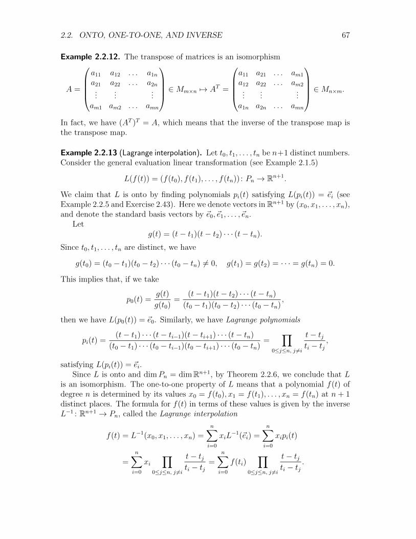
2.2. ONTO, ONE-TO-ONE, AND INVERSE 67
Example 2.2.12. The transpose of matrices is an isomorphism
A =
a11 a12 . . . a1n
a21 a22 . . . a2n...
......
am1 am2 . . . amn
∈Mm×n 7→ AT =
a11 a21 . . . am1
a12 a22 . . . am2...
......
a1n a2n . . . amn
∈Mn×m.
In fact, we have (AT )T = A, which means that the inverse of the transpose map isthe transpose map.
Example 2.2.13 (Lagrange interpolation). Let t0, t1, . . . , tn be n+1 distinct numbers.Consider the general evaluation linear transformation (see Example 2.1.5)
L(f(t)) = (f(t0), f(t1), . . . , f(tn)) : Pn → Rn+1.
We claim that L is onto by finding polynomials pi(t) satisfying L(pi(t)) = ~ei (seeExample 2.2.5 and Exercise 2.43). Here we denote vectors in Rn+1 by (x0, x1, . . . , xn),and denote the standard basis vectors by ~e0, ~e1, . . . , ~en.
Letg(t) = (t− t1)(t− t2) · · · (t− tn).
Since t0, t1, . . . , tn are distinct, we have
g(t0) = (t0 − t1)(t0 − t2) · · · (t0 − tn) 6= 0, g(t1) = g(t2) = · · · = g(tn) = 0.
This implies that, if we take
p0(t) =g(t)
g(t0)=
(t− t1)(t− t2) · · · (t− tn)
(t0 − t1)(t0 − t2) · · · (t0 − tn),
then we have L(p0(t)) = ~e0. Similarly, we have Lagrange polynomials
pi(t) =(t− t1) · · · (t− ti−1)(t− ti+1) · · · (t− tn)
(t0 − t1) · · · (t0 − ti−1)(t0 − ti+1) · · · (t0 − tn)=
∏0≤j≤n, j 6=i
t− tjti − tj
,
satisfying L(pi(t)) = ~ei.Since L is onto and dimPn = dimRn+1, by Theorem 2.2.6, we conclude that L
is an isomorphism. The one-to-one property of L means that a polynomial f(t) ofdegree n is determined by its values x0 = f(t0), x1 = f(t1), . . . , xn = f(tn) at n + 1distinct places. The formula for f(t) in terms of these values is given by the inverseL−1 : Rn+1 → Pn, called the Lagrange interpolation
f(t) = L−1(x0, x1, . . . , xn) =n∑i=0
xiL−1(~ei) =
n∑i=0
xipi(t)
=n∑i=0
xi∏
0≤j≤n, j 6=i
t− tjti − tj
=n∑i=0
f(ti)∏
0≤j≤n, j 6=i
t− tjti − tj
.

68 CHAPTER 2. LINEAR TRANSFORMATION
For example, a quadratic polynomial f(t) satisfying f(−1) = 1, f(0) = 2, f(1) = 3is uniquely given by
f(t) = 1t(t− 1)
(−1) · (−2)+ 2
(t+ 1)(t− 1)
1 · (−1)+ 3
(t+ 1)t
4 · 3= 2− 1
4t− 5
4t2.
Exercise 2.51. Suppose dimV = dimW and L : V → W is a linear transformation. Provethat the following are equivalent.
1. L is invertible.
2. L has left inverse: There is K : W → V , such that K ◦ L = I.
3. L has right inverse: There is K : W → V , such that L ◦K = I.
Moreover, show that the two K in the second and third parts must be the same.
Exercise 2.52. Explain dim Hom(V,W ) = dimV dimW .
Exercise 2.53. Explain that the linear transformation
f ∈ Pn 7→ (f(t0), f ′(t0), . . . , f (n)(t0)) ∈ Rn+1
is an isomorphism. What is the inverse isomorphism?
Exercise 2.54. Explain that the linear transformation (the right side has obvious vectorspace structure)
f ∈ C∞ 7→ (f ′, f(t0)) ∈ C∞ × R
is an isomorphism. What is the inverse isomorphism?
2.2.3 Invertible Matrix
A matrix A is invertible if the corresponding linear transformation L(~x) = A~x isinvertible (i.e., an isomorphism), and the inverse matrix A−1 is the matrix of theinverse linear transformation L−1. By Theorem 2.2.6 (and Theorems 1.3.14 and1.3.15), an invertible matrix must be a square matrix.
A linear transformation K is the inverse of L if L ◦ K = I and K ◦ L = I.Correspondingly, a matrix B is the inverse of A if AB = BA = I. Exercise 2.51shows that, in case of equal dimension, L ◦ K = I is equivalent to K ◦ L = I.Correspondingly, for square matrices, AB = I is equivalent to BA = I.
Example 2.2.14. Since the inverse of the identity linear transformation is the iden-tity, the inverse of the identity matrix is the identity matrix: I−1
n = In.

2.2. ONTO, ONE-TO-ONE, AND INVERSE 69
Example 2.2.15. The rotation Rθ of the plane by angle θ in Example 2.1.3 is in-vertible, with the inverse R−1
θ = R−θ being the rotation by angle −θ. Therefore thematrix of R−θ is the inverse of the matrix of Rθ(
cos θ − sin θsin θ cos θ
)−1
=
(cos θ sin θ− sin θ cos θ
).
One can directly verify that the multiplication of the two matrices is the identity.The flipping Fρ in Example 2.1.3 is also invertible, with the inverse F−1
ρ = Fρbeing the flipping itself. Therefore the matrix of Fρ is the inverse of itself (θ = 2ρ)(
cos θ sin θsin θ − cos θ
)−1
=
(cos θ sin θsin θ − cos θ
).
Exercise 2.55. Construct a 2 × 3 matrix A and a 3 × 2 matrix B satisfying AB = I2.Explain that BA can never be I3.
Exercise 2.56. What are the inverses of elementary matrices?
Exercise 2.57. Suppose A and B are invertible matrices. Prove that (AB)−1 = B−1A−1.
Exercise 2.58. Prove that the trace defined in Example 2.10 satisfies trAXA−1 = trX.
The following summarises many equivalent criteria for invertible matrix (andthere will be more).
Proposition 2.2.9. The following are equivalent for an n× n matrix A.
1. A is invertible.
2. A~x = ~b has solution for all ~b ∈ Rn.
3. The solution of A~x = ~b is unique.
4. The homogeneous system A~x = ~0 has only trivial solution ~x = ~0.
5. A~x = ~b has unique solution for all ~b ∈ Rn.
6. The columns of A span Rn.
7. The columns of A are linearly independent.
8. The columns of A form a basis of Rn.
9. All rows of A are pivot.
10. All columns of A are pivot.

70 CHAPTER 2. LINEAR TRANSFORMATION
11. The reduced row echelon form of A is the identity matrix I.
12. A is the product of elementary matrices.
Next we try to calculate the inverse matrix.
Let A be the matrix of an invertible linear transformation L : Rn → Rn. LetA−1 = (~w1 ~w2 · · · ~wn) be the matrix of the inverse linear transformation L−1. Then~wi = L−1(~ei) = A−1~ei. This implies A~wi = L(~wi) = ~ei. Therefore the i-th columnof A−1 is the solution of the system of linear equation A~x = ~ei. The solution can becalculated by the reduced row echelon form of the augmented matrix
(A ~ei)→ (I ~wi).
Here the row operations can reduce A to I by Proposition 2.2.9. Then the solutionof A~x = ~ei is exactly the last column of the reduced row echelon form (I ~wi).
Since the systems of liner equations A~x = ~e1, A~x = ~e2, . . . , A~x = ~en havethe same coefficient matrix A, we may solve these equations simultaneously bycombining the row operations
(A I) = (A ~e1 ~e2 · · · ~en)→ (I ~w1 ~w2 · · · ~wn) = (I A−1).
We have already used the idea in Example 1.3.17.
Example 2.2.16. The row operations in Example 2.1.20 give
(1 23 4
)−1
=
(−2 1
32−1
2
).
In general, we can directly verify that
(a bc d
)−1
=1
ad− bc
(d −b−c a
), ad 6= bc.
Example 2.2.17. The basis in Example 1.3.14 shows that the matrix
A =
1 4 72 5 83 6 10

2.2. ONTO, ONE-TO-ONE, AND INVERSE 71
is invertible. Then we carry out the row operations
(A I) =
1 4 7 1 0 02 5 8 0 1 03 6 10 0 0 1
→1 4 7 1 0 0
0 −3 −6 −2 1 00 −6 −11 −3 0 1
→
1 4 7 1 0 00 1 2 2
3−1
30
0 0 1 1 −2 1
→1 0 −1 −5
343
00 1 2 2
3−1
30
0 0 1 1 −2 1
→
1 0 0 −23−2
31
0 1 0 −43
113−2
0 0 1 1 −2 1
.
Therefore 1 4 72 5 83 6 10
−1
=
−23−2
31
−43
113−2
1 −2 1
.
Example 2.2.18. The row operation in Example 1.3.17 shows that 1 1 1−1 0 10 −1 1
−1
=1
3
1 −2 11 1 −21 1 1
.
In terms of linear transformation, the result means that the linear transformation
L
x1
x2
x3
=
x1 + x2 + x3
−x1 + x3
−x2 + x3
: R3 → R3
is invertible, and the inverse is
L−1
x1
x2
x3
=1
3
x1 − 2x2 + x3
x1 + x2 − 2x3
x1 + x2 + x3
: R3 → R3.
Exercise 2.59. What is the inverse of 1× 1 matrix (a)?
Exercise 2.60. Verify the formula for the inverse of 2 × 2 matrix in Example 2.2.16 bymultiplying the two matrices together. Moreover, show that the 2 × 2 matrix is notinvertible when ad = bc.
Exercise 2.61. Find inverse matrix.

72 CHAPTER 2. LINEAR TRANSFORMATION
1.
0 1 00 0 11 0 0
.
2.
0 0 1 01 0 0 00 0 0 10 1 0 0
.
3.
1 1 01 0 10 1 1
.
4.
1 1 1 01 1 0 11 0 1 10 1 1 1
.
5.
1 0 0a 1 0b c 1
.
6.
1 a b c0 1 a b0 0 1 a0 0 0 1
.
7.
b c 11 0 0a 1 0
.
8.
c a b 1b 1 a 0a 0 1 01 0 0 0
.
Exercise 2.62. Find the inverse matrix.
1.
1 1 1 · · · 10 1 1 · · · 10 0 1 · · · 1...
......
...0 0 0 · · · 1
.
2.
1 a1 a2 · · · an−1
0 1 a1 · · · an−2
0 0 1 · · · an−3...
......
...0 0 0 · · · 1
.
3.
0 0 · · · 0 10 0 · · · 1 a1
0 0 · · · a1 a2...
......
...1 a1 · · · an−2 an−1
.
2.3 Matrix of General Linear Transformation
By using bases to identify general vector spaces with Euclidean spaces, we mayintroduce the matrix of a general linear transformation with respect to bases.
2.3.1 Matrix with Respect to Bases
Let α = {~v1, ~v2, . . . , ~vn} and β = {~w1, ~w2, . . . , ~wm} be (ordered) bases of (finitedimensional) vector spaces V and W . Then a linear transformation L : V → W canbe translated into a linear transformation Lβα between Euclidean spaces.
VL−−−→ W
[·]α
y∼= ∼=y[·]β
Rn Lβα−−−→ Rn
Lβα([~v]α) = [L(~v)]β for ~v ∈ V.
Please pay attention to the notation, that Lβα is the corresponding linear transfor-mation from α to β.

2.3. MATRIX OF GENERAL LINEAR TRANSFORMATION 73
The matrix [L]βα of L with respect to bases α and β is the matrix of the lineartransformation Lβα, introduced in Section 2.1.2. To calculate this matrix, we applythe translation above to a vector ~vi ∈ α and use [~v]α = ~ei
~viL−−−→ L(~vi)y y
~eiLβα−−−→ [L(~vi)]β
Lβα(~ei) = Lβα([~vi]α) = [L(~vi)]β.
Denote L(α) = {L(~v1), L(~v2), . . . , L(~vn)}. Then we have
[L]βα = ([L(~v1)]β [L(~v2)]β · · · [L(~vn)]β) = [L(α)]β.
Specifically, suppose α = {~v1, ~v2} is a basis of V , and β = {~w1, ~w2, ~w3} is a basisof W . A linear transformation L : V → W is determined by
L(~v1) = a11 ~w1 + a21 ~w2 + a31 ~w3,
L(~v2) = a12 ~w1 + a22 ~w2 + a32 ~w3.
Then
[L(~v1)]β =
a11
a21
a31
, [L(~v2)]β =
a12
a22
a32
, [L]βα =
a11 a12
a21 a22
a31 a32
.
Note that the matrix [L]βα is obtained by combining all the coefficients in L(~v1),L(~v2) and then take the transpose.
Example 2.3.1. The orthogonal projection P of R3 to the plane x + y + z = 0 inExample 2.1.13 preserves vectors on the plan and maps vectors orthogonal to theplane to ~0. Specifically, with respect to the basis
α = {~v1, ~v2, ~v3}, ~v1 = (1,−1, 0), ~v2 = (1, 0,−1), ~v3 = (1, 1, 1),
we have
P (~v1) = ~v1, P (~v2) = ~v2, P (~v3) = ~0.
This means that
[P ]αα =
1 0 00 1 00 0 0
.
This is much simpler than the matrix with respect to the standard basis ε that weobtained in Example 2.1.13.

74 CHAPTER 2. LINEAR TRANSFORMATION
Example 2.3.2. With respect to the standard monomial bases α = {1, t, t2, t3}and β = {1, t, t2} of P3 and P2, the matrix of the derivative linear transformationD : P3 → P2 is
[D]βα = [(1)′, (t)′, (t2)′, (t3)′]{1,t,t2} = [0, 1, 2t, 3t2]{1,t,t2} =
0 1 0 00 0 2 00 0 0 3
.
For example, the derivative (1 + 2t+ 3t2 + 4t3)′ = 2 + 6t+ 12t2 fits into
2612
=
0 1 0 00 0 2 00 0 0 3
1234
.
If we modify the basis β to γ = {1, t− 1, (t− 1)2} in Example 1.3.3, then
[D]γα = [0, 1, 2t, 3t2]{1,t−1,(t−1)2}
= [0, 1, 2(1 + (t− 1)), 3(1 + (t− 1))2]{1,t−1,(t−1)2}
= [0, 1, 2 + 2(t− 1), 3 + 6(t− 1) + 3(t− 1)2]{1,t−1,(t−1)2}
=
0 1 2 30 0 2 60 0 0 3
.
Example 2.3.3. The linear transformation in Example 2.1.16
L(f) = (1 + t2)f ′′ + (1 + t)f ′ − f : P3 → P3
satisfies
L(1) = −1, L(t) = 1, L(t2) = 2 + 2t+ 3t2, L(t3) = 6t+ 3t2 + 8t3.
Therefore
[L]{1,t,t2,t3}{1,t,t2,t3} =
−1 1 2 00 0 2 60 0 3 30 0 0 8
.
To solve the equation L(f) = t+ 2t3 in Example 2.1.16, we have row operations−1 1 2 0 00 0 2 6 10 0 3 3 00 0 0 8 2
→−1 1 2 0 00 0 1 1 00 0 2 6 10 0 0 8 2
→−1 1 2 0 00 0 1 1 00 0 0 4 10 0 0 0 0
.

2.3. MATRIX OF GENERAL LINEAR TRANSFORMATION 75
This shows that L is not one-to-one and not onto. Moreover, the solution of thedifferential equation is given by
a3 = 14, a2 = −a3 = −1
4, a0 = 2 · 1
4+ a1 = 1
2+ a1.
In other words, the solution is (c = a1 is arbitrary)
f = 12
+ a1 + a1t− 14t2 + 1
4t3 = c(1 + t) + 1
4(2− t2 + t3).
Example 2.3.4. With respect to the standard basis of M2×2
σ = {S1, S2, S3, S4} =
{(1 00 0
),
(0 10 0
),
(0 01 0
),
(0 00 1
)},
the transpose linear transformation ·T : M2×2 →M2×2 has matrix
[·T ]σσ = [σT ]σ = [S1, S3, S2, S4]{S1,S2,S3,S4} =
1 0 0 00 0 1 00 1 0 00 0 0 1
.
Moreover, the linear transformation A· : M2×2 → M2×2 of left multiplying by A =(1 23 4
)has matrix
[A·]σσ = [Aσ]σ = [AS1, AS2, AS3, AS4]{S1,S2,S3,S4}
= [S1 + 3S3, S2 + 3S4, 2S1 + 4S3, 2S2 + 4S4]{S1,S2,S3,S4} =
1 0 2 00 1 0 23 0 4 00 3 0 4
.
Exercise 2.63. In Example 2.3.2, what is the matrix of the derivative linear transformationif α is changed to {1, t+ 1, (t+ 1)2}?
Exercise 2.64. Find the matrix of∫ t
0 : P2 → P3, with respect to the usual bases in P2 and
P3. What about∫ t
1 : P2 → P3?
Exercise 2.65. In Example 2.3.4, find the matrix of the right multiplication by A.
Proposition 2.3.1. The matrix of linear transformation has the following properties
[I]αα = I, [L+K]βα = [L]βα + [K]βα, [cL]βα = c[L]βα,
[L ◦K]γα = [L]γβ[K]βα.

76 CHAPTER 2. LINEAR TRANSFORMATION
Proof. The equality [I]αα = I is equivalent to that Iαα is the identity linear trans-formation. This follows from
Iαα([~v]α) = [I(~v)]α = [~v]α.
Alternatively, we have[I]αα = [α]α = I.
The equality [L+K]βα = [L]βα+[K]βα is equivalent to the equality (L+K)βα =Lβα+Kβα for linear transformations, which we can verify by using Proposition 1.3.2
(L+K)βα([~v]α) = [(L+K)(~v)]β = [L(~v) +K(~v)]β
= [L(~v)]β + [K(~v)]β = Lβα([~v]α) +Kβα([~v]α).
Alternatively, we have (the second equality is true for individual vectors in α)
[L+K]βα = [(L+K)(α)]β = [L(α) +K(α)]β
= [L(α)]β + [K(α)]β = [L]βα + [K]βα.
The verification of [cL]βα = c[L]βα is similar, and is omitted.The equality [L◦K]γα = [L]γβ[K]βα is equivalent to (L◦K)γα = Lγβ ◦Kβα. This
follows from
(L ◦K)γα([~v]α) = [(L ◦K)(~v)]γ = [L(K(~v))]γ
= Lγβ([K(~v)]β) = Lγβ(Kβα([~v]α)) = (Lγβ ◦Kβα)([~v]α).
Alternatively, we have (the third equality is true for individual vectors in K(α))
[L ◦K]γα = [(L ◦K)(α)]γ = [L(K(α))]γ = [L]γβ[K(α)]β = [L]γβ[K]βα.
Example 2.3.5 (Vandermonde Matrix). Applying the evaluation linear transforma-tion in Example 2.2.13 to the monomials, we get the matrix of the linear transfor-mation
[L]ε{1,t,...,tn} =
1 t0 t20 . . . tn01 t1 t21 . . . tn11 t2 t22 . . . tn2...
......
...1 tn t2n . . . tnn
.
This is called the Vandermonde matrix. Example 2.2.13 tells us that the matrixis invertible if and only if all ti are distinct. Moreover, the Lagrangian interpola-tion is the formula for L−1, and shows that the i-th column of the inverse of theVandermonde matrix is the coefficients in the polynomial
L−1(~ei) =(t− t1) · · · (t− ti−1)(t− ti+1) · · · (t− tn)
(t0 − t1) · · · (t0 − ti−1)(t0 − ti+1) · · · (t0 − tn).
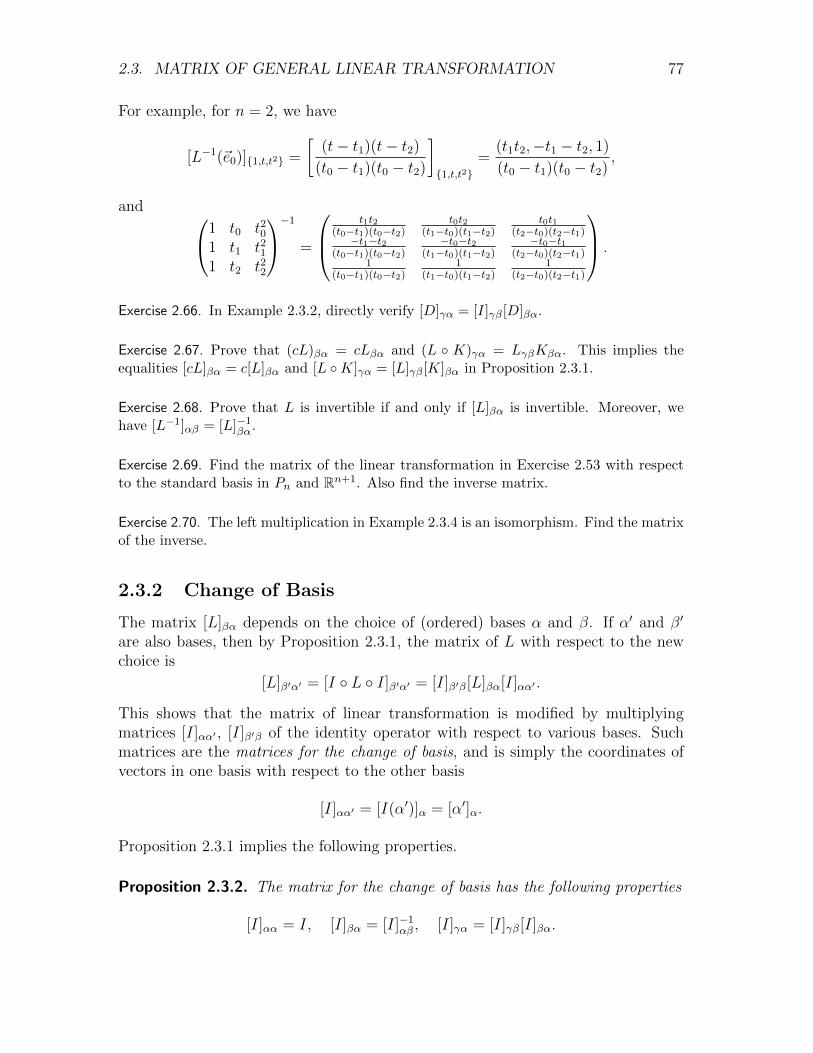
2.3. MATRIX OF GENERAL LINEAR TRANSFORMATION 77
For example, for n = 2, we have
[L−1(~e0)]{1,t,t2} =
[(t− t1)(t− t2)
(t0 − t1)(t0 − t2)
]{1,t,t2}
=(t1t2,−t1 − t2, 1)
(t0 − t1)(t0 − t2),
and 1 t0 t201 t1 t211 t2 t22
−1
=
t1t2
(t0−t1)(t0−t2)t0t2
(t1−t0)(t1−t2)t0t1
(t2−t0)(t2−t1)−t1−t2
(t0−t1)(t0−t2)−t0−t2
(t1−t0)(t1−t2)−t0−t1
(t2−t0)(t2−t1)1
(t0−t1)(t0−t2)1
(t1−t0)(t1−t2)1
(t2−t0)(t2−t1)
.
Exercise 2.66. In Example 2.3.2, directly verify [D]γα = [I]γβ[D]βα.
Exercise 2.67. Prove that (cL)βα = cLβα and (L ◦ K)γα = LγβKβα. This implies theequalities [cL]βα = c[L]βα and [L ◦K]γα = [L]γβ[K]βα in Proposition 2.3.1.
Exercise 2.68. Prove that L is invertible if and only if [L]βα is invertible. Moreover, wehave [L−1]αβ = [L]−1
βα.
Exercise 2.69. Find the matrix of the linear transformation in Exercise 2.53 with respectto the standard basis in Pn and Rn+1. Also find the inverse matrix.
Exercise 2.70. The left multiplication in Example 2.3.4 is an isomorphism. Find the matrixof the inverse.
2.3.2 Change of Basis
The matrix [L]βα depends on the choice of (ordered) bases α and β. If α′ and β′
are also bases, then by Proposition 2.3.1, the matrix of L with respect to the newchoice is
[L]β′α′ = [I ◦ L ◦ I]β′α′ = [I]β′β[L]βα[I]αα′ .
This shows that the matrix of linear transformation is modified by multiplyingmatrices [I]αα′ , [I]β′β of the identity operator with respect to various bases. Suchmatrices are the matrices for the change of basis, and is simply the coordinates ofvectors in one basis with respect to the other basis
[I]αα′ = [I(α′)]α = [α′]α.
Proposition 2.3.1 implies the following properties.
Proposition 2.3.2. The matrix for the change of basis has the following properties
[I]αα = I, [I]βα = [I]−1αβ , [I]γα = [I]γβ[I]βα.

78 CHAPTER 2. LINEAR TRANSFORMATION
Example 2.3.6. Let ε be the standard basis of Rn, and let α = {~v1, ~v2, . . . , ~vn} beanother basis. Then the matrix for changing from α to ε is
[I]εα = [α]ε = (~v1 ~v2 · · · ~vn) = (α).
In general, the matrix for changing from α to β is
[I]βα = [I]βε[I]εα = [I]−1εβ [I]εα = [β]−1
ε [α]ε = (β)−1(α).
For example, the matrix for changing from the basis in Example 2.2.17
α = {(1, 2, 3), (4, 5, 6), (7, 8, 10)}
to the basis in Examples 1.3.17, 2.2.18 and 2.3.1
β = {(1,−1, 0), (1, 0,−1), (1, 1, 1)}
is 1 1 1−1 0 10 −1 1
−11 4 72 5 83 6 10
=1
3
1 −2 11 1 −21 1 1
1 4 72 5 83 6 10
=1
3
0 0 1−3 −3 −56 15 25
.
Example 2.3.7. Consider the basis αθ = {(cos θ, sin θ), (− sin θ, cos θ)} of unit lengthvectors on the plane at angles θ and θ+ π
2. The matrix for the change of basis from
αθ1 to αθ2 is obtained from the αθ2-coordinates of vectors in αθ1 . Since αθ1 is obtainedfrom αθ2 by rotating θ = θ1 − θ2, the coordinates are the same as the ε-coordinatesof vectors in αθ. This means
[I]αθ2αθ1 =
(cos θ − sin θsin θ cos θ
)=
(cos(θ1 − θ2) − sin(θ1 − θ2)sin(θ1 − θ2) cos(θ1 − θ2)
).
This is consistent with the formula in Example 2.3.6
[I]αθ2αθ1 = (αθ2)−1(αθ1) =
(cos θ2 − sin θ2
sin θ2 cos θ2
)−1(cos θ1 − sin θ1
sin θ1 cos θ1
).
Example 2.3.8. The matrix for the change from the basis α = {1, t, t2, t3} of P3 toanother basis β = {1, t− 1, (t− 1)2, (t− 1)3} is
[I]βα = [1, t, t2, t3]{1,t−1,(t−1)2,(t−1)3}
= [1, 1 + (t− 1), 1 + 2(t− 1) + (t− 1)2,
1 + 3(t− 1) + 3(t− 1)2 + (t− 1)3]{1,t−1,(t−1)2,(t−1)3}
=
1 1 1 10 1 2 30 0 1 30 0 0 1
.

2.3. MATRIX OF GENERAL LINEAR TRANSFORMATION 79
The inverse of this matrix is
[I]αβ = [1, t− 1, (t− 1)2, (t− 1)3]{1,t,t2,t3}
= [1,−1 + t, 1− 2t+ t2,−1 + 3t− 3t2 + t3]{1,t,t2,t3}
=
1 −1 1 −10 1 −2 30 0 1 −30 0 0 1
.
We can also use the method outlined before Example 2.2.16 to calculate the inverse.But the method above is simpler.
The equality
(t+ 1)3 = 1 + 3t+ 3t2 + t3 = ((t− 1) + 2)3 = 8 + 12(t− 1) + 6(t− 1)2 + (t− 1)3
gives coordinates
[(t+ 1)3]α = (1, 3, 3, 1), [(t+ 1)3]β = (8, 12, 6, 1).
The two coordinates are related by the matrices for the change of basis81261
=
1 1 1 10 1 2 30 0 1 30 0 0 1
1331
,
1331
=
1 −1 1 −10 1 −2 30 0 1 −30 0 0 1
81261
.
Exercise 2.71. Use matrices for the change of basis in Example 2.3.8 to find the matrix[L]{1,t,t2,t3}{1,t−1,(t−1)2,(t−1)3} of the linear transformation L in Example 2.3.3.
Exercise 2.72. If the basis in the source vector space V is changed by one of three operationsin Exercise 1.59, how is the matrix of linear transformation changed? What about thesimilar change in the target vector space W?
2.3.3 Similar Matrix
For a linear operator L : V → V , we usually choose the same basis α for the domainV and the range V . The matrix of the linear operator with respect to the basis α is[L]αα. The matrices with respect to different bases are related by
[L]ββ = [I]βα[L]αα[I]αβ = [I]−1αβ [L]αα[I]αβ = [I]βα[L]αα[I]−1
βα.
We say the two matrices A = [L]αα and B = [L]ββ are similar in the sense that theyare related by
B = P−1AP = QAQ−1,
where P (matrix for changing from β to α) is an invertible matrix with P−1 = Q(matrix for changing from α to β).

80 CHAPTER 2. LINEAR TRANSFORMATION
Example 2.3.9. In Example 2.3.1, we showed that the matrix of the orthogonalprojection P in Example 2.1.13 with respect to α = {(1,−1, 0), (1, 0,−1), (1, 1, 1)}is very simple
[P ]αα =
1 0 00 1 00 0 0
.
On the other hand, by Examples 2.3.6 and 2.2.18, we have
[I]εα = [α]ε =
1 1 1−1 0 10 −1 1
, [I]−1εα =
1
3
1 −2 11 1 −21 1 1
.
Then we get the usual matrix of P (with respect the the standard basis ε)
[P ]εε = [I]εα[P ]αα[I]−1εα
=
1 1 1−1 0 10 −1 1
1 0 00 1 00 0 0
1 1 1−1 0 10 −1 1
−1
=1
3
2 −1 −1−1 2 −1−1 −1 2
.
The matrix is the same as the one obtained in Example 2.1.13 by another method.
Example 2.3.10. Consider the linear operator L(f(t)) = tf ′(t) + f(t) : P3 → P3.Applying the operator to the bases α = {1, t, t2, t3}, we get
L(1) = 1, L(t) = 2t, L(t2) = 3t2, L(t3) = 4t3.
Therefore
[L]αα =
1 0 0 00 2 0 00 0 3 00 0 0 4
.
Consider another basis β = {1, t− 1, (t− 1)2, (t− 1)3} of P2. By Example 2.3.8,we have
[I]βα =
1 1 1 10 1 2 30 0 1 30 0 0 1
, [I]αβ =
1 −1 1 −10 1 −2 30 0 1 −30 0 0 1
.
Therefore
[L]ββ = [I]βα[L]αα[I]αβ
=
1 1 1 10 1 2 30 0 1 30 0 0 1
1 0 0 00 2 0 00 0 3 00 0 0 4
1 −1 1 −10 1 −2 30 0 1 −30 0 0 1
=
1 1 0 00 2 2 00 0 3 30 0 0 4
.

2.4. DUAL 81
We can verify the result by directly applying L(f) = (tf(t))′ to vectors in β
L(1) = 1,
L(t− 1) = [(t− 1) + (t− 1)2]′ = 1 + 2(t− 1),
L((t− 1)2) = [(t− 1)2 + (t− 1)3]′ = 2(t− 1) + 3(t− 1)2,
L((t− 1)3) = [(t− 1)3 + (t− 1)4]′ = 3(t− 1)2 + 4(t− 1)3.
Exercise 2.73. Explain that if A is similar to B, then B is similar to A.
Exercise 2.74. Explain that if A is similar to B, and B is similar to C, then A is similarto C.
Exercise 2.75. Find the matrix of the linear operator of R2 that sends ~v1 = (1, 2) and~v2 = (3, 4) to 2~v1 and 3~v2. What about sending ~v1, ~v2 to ~v2, ~v1?
Exercise 2.76. Find the matrix of the reflection of R3 with respect to the plane x+y+z = 0.
Exercise 2.77. Find the matrix of the linear operator of R3 that circularly sends the basisvectors in Example 2.1.13 to each other
(1,−1, 0) 7→ (1, 0,−1) 7→ (1, 1, 1) 7→ (1,−1, 0).
2.4 Dual
2.4.1 Dual Space
A function on a vector space V is a map l : V → R. If the map is a linear transfor-mation
l(~u+ ~v) = l(~u) + l(~v), l(c~u) = c l(~u),
then we call the map a linear functional. All the linear functionals on a vector spaceV form a vector space, called the dual space
V ∗ = Hom(V,R).
An ordered bases α = {~v1, ~v2, . . . , ~vn} of V gives an isomorphism
l ∈ V ∗ ←→ l(α) = (l(~v1), l(~v2), . . . , l(~vn)) = (a1, a2, . . . , an) ∈ Rn. (2.4.1)
The 1 × n matrix on the right is the matrix [l(α)]1 = [l]1α of l with respect to thebasis α of V and the basis 1 of R. The formula for l (i.e., the inverse of (2.4.1)) isthen given by (2.1.1)
l(~x) = a1x1 + a2x2 + · · ·+ anxn, [~x]α = (x1, x2, . . . , xn). (2.4.2)

82 CHAPTER 2. LINEAR TRANSFORMATION
The isomorphism tells usdimV ∗ = dimV. (2.4.3)
Under the isomorphism (2.4.1), the standard basis ε of Rn corresponds to abasis α∗ = {~v∗1, ~v∗2, . . . , ~v∗n} of V ∗, called the dual basis. The correspondence means(~v∗i (~v1), ~v∗i (~v2), . . . , ~v∗i (~vn)) = ~ei, or
~v∗i (~vj) = δij =
{1, if i = j,
0, if i 6= j,
In other words, the linear functional ~v∗i is the i-th α-coordinate
~v∗i (x1~v1 + x2~v2 + · · ·+ xn~vn) = xi.
For ~x = x1~v1 + x2~v2 + · · ·+ xn~vn, we can also write this as
[~x]α = (~v∗1(~x), ~v∗2(~x), . . . , ~v∗n(~x)) = α∗(~x),
or~x = ~v∗1(~x)~v1 + ~v∗2(~x)~v2 + · · ·+ ~v∗n(~x)~vn.
Proposition 2.4.1. Suppose V is a finite dimensional vector space, and ~x, ~y ∈ V .Then ~x = ~y if and only if l(~x) = l(~y) for all l ∈ V ∗.
For the sufficiency, we take l to be ~v∗i and get [~x]α = [~y]α. Since the coordinatemap is an isomorphism, this implies ~x = ~y.
We may also interpret (2.4.2) as
[l]α∗ = (l(~v1), l(~v2), . . . , l(~vn)) = l(α),
orl = l(~v1)~v∗1 + l(~v2)~v∗2 + · · ·+ l(~vn)~v∗n.
Example 2.4.1. The dual basis of the standard basis of Euclidean space is given by
~e∗i (x1, x2, . . . , xn) = xi.
The isomorphism (2.4.1) is given by
l(x1, x2, . . . , xn) = a1x2 + a2x2 + · · ·+ anxn ∈ (Rn)∗ ←→ (a1, a2, . . . , an) ∈ Rn.
Example 2.4.2. We want to calculate the dual basis of the basis α = {~v1, ~v2, ~v3} ={(1,−1, 0), (1, 0,−1), (1, 1, 1)} in Example 1.3.17. The dual basis vector
~v∗1(x1, x2, x3) = a1x1 + a2x2 + a3x3
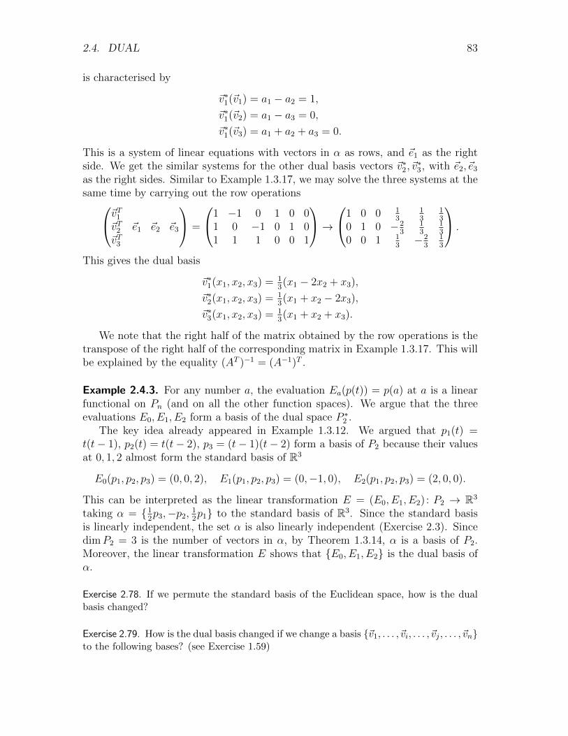
2.4. DUAL 83
is characterised by
~v∗1(~v1) = a1 − a2 = 1,
~v∗1(~v2) = a1 − a3 = 0,
~v∗1(~v3) = a1 + a2 + a3 = 0.
This is a system of linear equations with vectors in α as rows, and ~e1 as the rightside. We get the similar systems for the other dual basis vectors ~v∗2, ~v
∗3, with ~e2, ~e3
as the right sides. Similar to Example 1.3.17, we may solve the three systems at thesame time by carrying out the row operations~vT1~vT2 ~e1 ~e2 ~e3
~vT3
=
1 −1 0 1 0 01 0 −1 0 1 01 1 1 0 0 1
→1 0 0 1
313
13
0 1 0 −23
13
13
0 0 1 13−2
313
.
This gives the dual basis
~v∗1(x1, x2, x3) = 13(x1 − 2x2 + x3),
~v∗2(x1, x2, x3) = 13(x1 + x2 − 2x3),
~v∗3(x1, x2, x3) = 13(x1 + x2 + x3).
We note that the right half of the matrix obtained by the row operations is thetranspose of the right half of the corresponding matrix in Example 1.3.17. This willbe explained by the equality (AT )−1 = (A−1)T .
Example 2.4.3. For any number a, the evaluation Ea(p(t)) = p(a) at a is a linearfunctional on Pn (and on all the other function spaces). We argue that the threeevaluations E0, E1, E2 form a basis of the dual space P ∗2 .
The key idea already appeared in Example 1.3.12. We argued that p1(t) =t(t− 1), p2(t) = t(t− 2), p3 = (t− 1)(t− 2) form a basis of P2 because their valuesat 0, 1, 2 almost form the standard basis of R3
E0(p1, p2, p3) = (0, 0, 2), E1(p1, p2, p3) = (0,−1, 0), E2(p1, p2, p3) = (2, 0, 0).
This can be interpreted as the linear transformation E = (E0, E1, E2) : P2 → R3
taking α = {12p3,−p2,
12p1} to the standard basis of R3. Since the standard basis
is linearly independent, the set α is also linearly independent (Exercise 2.3). SincedimP2 = 3 is the number of vectors in α, by Theorem 1.3.14, α is a basis of P2.Moreover, the linear transformation E shows that {E0, E1, E2} is the dual basis ofα.
Exercise 2.78. If we permute the standard basis of the Euclidean space, how is the dualbasis changed?
Exercise 2.79. How is the dual basis changed if we change a basis {~v1, . . . , ~vi, . . . , ~vj , . . . , ~vn}to the following bases? (see Exercise 1.59)
84 CHAPTER 2. LINEAR TRANSFORMATION
1. {~v1, . . . , ~vj , . . . , ~vi, . . . , ~vn}.
2. {~v1, . . . , c~vi, . . . , ~vn}, c 6= 0.
3. {~v1, . . . , ~vi + c~vj , . . . , ~vj , . . . , ~vn}.
Exercise 2.80. Find the dual basis of a basis {(a, b), (c, d)} of R2.
Exercise 2.81. Find the dual basis of the basis {(1, 2, 3), (4, 5, 6), (7, 8, 10)} of R3.
Exercise 2.82. Find the dual basis of the basis {1− t, 1− t2, 1 + t+ t2} of P2.
Exercise 2.83. Find the dual basis of the basis {1, t, t2} of P2. Moreover, express the dualbasis in the form l(p(t)) =
∫ 10 p(t)λ(t)dt for suitable λ(t) ∈ P2.
Exercise 2.84. Find the basis of P2, such that the dual basis is the evaluations at threedistinct places t1, t2, t3. Moreover, extend your result to Pn.
Exercise 2.85. Find the basis of P2, such that the dual basis is the three derivatives at 0:p(t) 7→ p(0), p(t) 7→ p′(0), p(t) 7→ p′′(0). Extend to the derivatives up to n-order for Pn,and at a place a other than 0.
2.4.2 Dual Linear Transformation
A linear transformation L : V → W induces the dual linear transformation
L∗(l) = l ◦ L : W ∗ → V ∗, (L∗(l))(~v) = l(L(~v)).
This is the special case U = R of Exercise 2.13 (and therefore justifies that L∗ isa linear transformation). The following shows that the dual linear transformationcorresponds to the transpose of matrix.
Proposition 2.4.2. Suppose α, β are bases of V,W , and α∗, β∗ are the correspondingdual bases of V ∗,W ∗. Then
[L∗]α∗β∗ = [L]Tβα.
Proof. For 1 ≤ i ≤ m = dimW and 1 ≤ j ≤ n = dimV , denote (notice ji for L∗)
α = {~v1, ~v2, . . . , ~vn}, β = {~w1, ~w2, . . . , ~wm}, [L]βα = (aij), [L∗]α∗β∗ = (a∗ji).
Then (recall the 3× 2 matrix of L before Example 2.3.1)
L(~vj) = a1j ~w1 + a2j ~w2 + · · ·+ amj ~wm,
L∗(~w∗i ) = a∗1i~v∗1 + a∗2i~v
∗2 + · · ·+ a∗ni~v
∗n.

2.4. DUAL 85
Applying the linear functional ~w∗i to the first equality, and applying the secondequality to ~vj, we get
~w∗i (L(~vj)) = aij, (L∗(~w∗i ))(~vj) = a∗ji.
By the definition of L∗, we have (L∗(~w∗i ))(~vj) = ~w∗i (L(~vj)). Therefore aij = a∗ji.This means [L]Tβα = [L∗]α∗β∗ .
By Exercise 2.13, the dual linear transformation has the following properties
I∗ = I, (L+K)∗ = L∗ +K∗, (cL)∗ = cL∗, (L ◦K)∗ = K∗ ◦ L∗.
Then by Proposition 2.4.2, these translate into properties of the transpose of matrix
IT = I, (A+B)T = AT +BT , (cA)T = cAT , (AB)T = BTAT .
Exercise 2.86. Directly verify that L∗(l) : W ∗ → V ∗ is a linear transformation: L∗(l+k) =L∗(l) + L∗(k), L∗(cl) = cL∗(l).
Exercise 2.87. Directly verify that the dual linear transformation has the claimed proper-ties: I∗(l) = l, (L+K)∗(l) = L∗(l) +K∗(l), (cL)∗(l) = cL∗(l), (L ◦K)∗(l) = K∗(L∗(l)).
By the last statements of Propositions 2.2.3 and 2.2.4, we know that L ◦K = Iimplies L is onto and K is one-to-one. Applying the dual switches the order intoK∗ ◦ L∗ = I. This suggests that K∗ is onto and L∗ is one-to-one, and almost givesthe proof of the following result.
Proposition 2.4.3. Suppose L : V → W is a linear transformation between finitedimensional vector spaces.
1. If L is onto, then L∗ is one-to-one.
2. If L is one-to-one, then L∗ is onto.
Proof. Suppose L is onto, and l, k ∈ V ∗ satisfy L∗(l) = L∗(k). Then l(L(~v)) =L∗(l)(~v) = L∗(k)(~v) = k(L(~v)) for all ~v ∈ V . Since L is onto, every vector of W isof the form L(~v) for some ~v ∈ V . Therefore the equality means l(~w) = k(~w) for all~w ∈ W . This is the definition of l = k, and proves the first statement.
The following proves the second statement
L is one-to-one =⇒ K ◦ L = I (Proposition 2.2.4)
=⇒ L∗ ◦K∗ = I ((L ◦K)∗ = K∗ ◦ L∗)=⇒ L∗ is onto. (Proposition 2.2.3)
In fact, we may also use the similar idea to prove the first statement.

86 CHAPTER 2. LINEAR TRANSFORMATION
Exercise 2.88. Let A be an m× n matrix. What is the relation between the existence andthe uniqueness of solutions of the following two systems of linear equations?
1. A~x = ~b: m equations in n variables.
2. AT~y = ~c: n equations in m variables.
Exercise 2.89. By Proposition 2.4.3, what can you say about the pivots of the row echelonforms of a matrix A and its transpose AT ? Note that row operation on AT can also beregarded as column operation on A.
Exercise 2.90. Do we really need to assume finite dimension in Proposition 2.4.3?
2.4.3 Double Dual
Any vector ~v ∈ V induces a function on the dual space V ∗
~v∗∗(l) = l(~v).
As the special case W = R of Exercise 2.11, the function ~v∗∗ is a linear functionalon V ∗. Therefore ~v∗∗ is a vector in the double dual V ∗∗ = (V ∗)∗ of the dual spaceV ∗. This gives the natural double dual map
~v ∈ V 7→ ~v∗∗ ∈ V ∗∗.
The following shows that the double dual map is a linear transformation
(a~v + b~w)∗∗(l) = l(a~v + b~w) = al(~v) + bl(~w) = a~v∗∗(l) + b~w∗∗(l) = (a~v∗∗ + b~w∗∗)(l).
Proposition 2.4.1 can be interpreted as ~v∗∗(l) = ~w∗∗(l) for all l implying ~v = ~w.Therefore the double dual map V 7→ V ∗∗ is one-to-one. By using (2.4.3) twice, weget dimV ∗∗ = dimV . Then by Theorem 2.2.6, we conclude that the double dualmap is an isomorphism.
Proposition 2.4.4. The double dual of a finite dimensional vector space is naturallyisomorphic to itself.
A linear transformation L : V → W induces a linear transformation L∗ : W ∗ →V ∗, which further induces the double dual linear transformation
L∗∗ : V ∗∗ → W ∗∗.
Let us compare with the natural isomorphism in Proposition 2.4.4
VL−−−→ W
∼=y y∼=V ∗∗
L∗∗−−−→ W ∗∗

2.4. DUAL 87
The following shows that L∗∗ can be identified with L under the natural isomorphism(~v ∈ V and l ∈ W ∗)
L∗∗(~v∗∗)(l) = ~v∗∗(L∗(l)) = (L∗(l))(~v) = l(L(~v)) = (L(~v))∗∗(l).
Therefore like Proposition 2.4.4, the double dual L∗∗ of a linear transformation L isnaturally identified with the linear transformation L itself.
Let A = [L]βα be the matrix of a linear transformation. Then by Proposition2.4.2, we have AT = [L∗]α∗β∗ , and (AT )T = [L∗∗]β∗∗α∗∗ (Exercise 2.91 implicitly used).The natural identification of L∗∗ and L is then an elaborately way of explaining(AT )T = A.
Combining the natural identification of L∗∗ and L with Proposition 2.4.3 givesthe following more complete result.
Theorem 2.4.5. Suppose L : V → W is a linear transformation between finite di-mensional vector spaces.
1. L is onto if and only if L∗ is one-to-one.
2. L is one-to-one if and only if L∗ is onto.
Exercise 2.91. For a basis α = {~v1, ~v2, . . . , ~vn} of V , the notation α∗∗ = {~v∗∗1 , ~v∗∗2 , . . . , ~v∗∗n }has two possible meanings.
1. (α∗)∗: First get dual basis α∗ of V ∗. Then get the dual of the dual basis (α∗)∗ of(V ∗)∗.
2. α∗∗: The image under the natural transformation V → V ∗∗.
Explain that the two meanings are the same.
2.4.4 Dual Pairing
A function b : V ×W → R is bilinear if it is linear in V and also linear in W
b(x1~v1 + x2~v2, ~w) = x1b(~v1, ~w) + x2b(~v2, ~w),
b(~v, y1 ~w1 + y2 ~w2) = y1b(~v, ~w1) + y2b(~v, ~w2).
Let α = {~v1, ~v2, . . . , ~vm} and β = {~w1, ~w2, . . . , ~wn} be bases of V and W . Thenthe bilinear property imples
b(x1~v1 + x2~v2 + · · ·+ xm~vm, y1 ~w1 + y2 ~w2 + · · ·+ yn ~wn) =∑
1≤i≤m1≤j≤n
xiyjb(~vi, ~wj).
Denote the matrix of bilinear function with respect to the bases
[b]αβ = (bij), bij = b(~vi, ~wj).

88 CHAPTER 2. LINEAR TRANSFORMATION
Then we haveb(~x, ~y) =
∑i,j
bijxiyj = [~x]Tα [b]αβ[~y]β.
We can define the linear combination of bilinear functions in the obvious way
(c1 b1 + c2 b2)(~x, ~y) = c1 b1(~x, ~y) + c1 b2(~x, ~y).
This makes all the bilinear functions on V ×W into a vector space. It is also easyto see that
[c1 b1 + c2 b2]αβ = c1[b1]αβ + c2[b2]αβ.
Therefore the vector space of bilinear functions is isomorphic to the vector space ofm× n matrices, m = dimV , n = dimW .
For a bilinear function b(~x, ~y) on V ×W , the linearity in V gives a map
~y ∈ W 7→ b(·, ~y) ∈ V ∗.
Then the linearity in W implies that the map is a linear transformation. Conversely,a linear transformation L : W → V ∗, gives a bilinear function
b(~x, ~y) = L(~y)(~x).
Here L(~y) is a linear functional on V and can be applied to ~x. This gives anisomorphism between the vector space of all bilinear functions on V ×W and thevector space Hom(W,V ∗).
Due to the symmetry in V and W , we also have the isomorphism between thevector space of all bilinear functions on V ×W and the vector space Hom(V,W ∗).One direction is given by
~x ∈ V 7→ K(~x) = b(~x, ·) ∈ W ∗.
The converse is given by
K ∈ Hom(V,W ∗) 7→ b(~x, ~y) = K(~x)(~y).
Example 2.4.4. The evaluation pairing
e(~x, l) = l(~x) : V × V ∗ → R
is a bilinear function. The corresponding linear transformation in Hom(V ∗, V ∗) isthe identity. The corresponding linear transformation in Hom(V, (V ∗)∗) is the doubledual map ~v 7→ ~v∗∗.
Let α and β be bases of V and V ∗. Then [e]αβ = I if and only if β is the dualbasis of α.
Exercise 2.92. Explain that two bilinear functions on V ×W are equal if and only if theyare equal on two spanning sets of V and W .

2.4. DUAL 89
Exercise 2.93. How is the matrix of a bilinear function changed when the bases are changed?
Exercise 2.94. Prove that L ∈ Hom(W,V ∗) and K ∈ Hom(V,W ∗) give the same bilinearfunction on V ×W if and only if K = L∗, subject to the isomorphism in Proposition 2.4.4.
Exercise 2.95. A bilinear function b on V ×W corresponds to L ∈ Hom(W,V ∗) and K ∈Hom(V,W ∗). Let α, β be bases of V,W , and α∗, β∗ be the dual bases. How are thematrices [b]αβ, [L]α∗β, [K]β∗α related?
Exercise 2.96. For a bilinear function b(~v, ~w) on V ×W , bt(~w,~v) = b(~v, ~w) is a bilinearfunction on W × V . Let α, β be bases of V,W . How are the matrices [b]αβ and [bt]βαrelated? Moreover, the linear functions b and bt correspond to four linear transformations.How are these linear transformations related?
Exercise 2.97. Let b(~x, ~y) be a bilinear function on V ×W . Let L : U → V be a lineartransformation.
1. Explain that b(L(~z), ~y) is a bilinear function on U ×W .
2. Given bases for U, V,W , how are the matrices of b(~x, ~y) and b(L(~z), ~y) related?
3. The two bilinear functions correspond to four linear transformations. How are theselinear transformations related?
Finally, please study the same problem for b(~x, L(~z)).
Definition 2.4.6. A bilinear function b : V ×W → R is a dual pairing if both inducedlinear transformations V → W ∗ and W → V ∗ are isomorphisms.
By Exercise 2.94, the two linear transformations can be regarded as dual toeach other. Therefore we only need one of them to be isomorphic. Moreover, byProposition 2.4.5, the dual pairing is equivalent to both V → W ∗ and W → V ∗
being onto, and is also equivalent to both being one-to-one.The evaluation pairing in Example 2.4.4 is a basic example of dual pairing. Using
the same idea, a basis α = {~v1, ~v2, . . . , ~vn} of V and a basis β = {~w1, ~w2, . . . , ~wn} ofW are dual bases with respect to the dual pairing b if
b(~vi, ~wj) = δij, or [b]αβ = I.
This is equivalent to that the corresponding V → W ∗ maps the basis α of V to thedual basis β∗ of W ∗, and is also equivalent to that the corresponding W → V ∗ mapsthe basis β of W to the dual basis α∗ of V ∗. The dual bases with respect to thebilinear function also give
~x = b(~x, ~w1)~v1 + b(~x, ~w2)~v2 + · · ·+ b(~x, ~wn)~vn for any ~x ∈ V,~y = b(~v1, ~y)~w1 + b(~v2, ~y)~w2 + · · ·+ b(~vn, ~y)~wn for any ~y ∈ W.

90 CHAPTER 2. LINEAR TRANSFORMATION
Exercise 2.98. Prove that a bilinear function is a dual pairing if and only if its matrix withrespect to some bases is invertible.

Chapter 3
Subspace
As human civilisation became more sophisticated, they found it necessary to extendtheir number systems. The ancient Greeks found that the rational numbers Q wasnot sufficient for describing lengths in geometry, and the problem was solved laterby the Arabs who extended the rational numbers to the real numbers R. Then theItalians found it useful to take the square root of −1 in their search for the rootsof cubic equations, and the idea led to the extension of real numbers to complexnumbers C.
In extending the number system, we still wish to preserve the key features of theold system. This means that the inclusions Q ⊂ R ⊂ C are compatible with the fourarithmetic operations. In other words, 2 + 3 = 5 is an equality of rational numbers,and is also an equality of real (or complex) numbers. In this sense, we may call Qa sub-number system of R and C.
3.1 Definition
3.1.1 Subspace
Definition 3.1.1. A subset H of a vector space V is a subspace if it satisfies
~u,~v ∈ H, a, b ∈ R =⇒ a~u+ b~v ∈ H.
Using the addition and scalar multiplication of V , the subset H is also a vectorspace. One should imagine that a subspace is a flat and infinite (with the onlyexception of the trivial subspace {~0}) subset passing through the origin.
The smallest subspace is the trivial subspace. The biggest subspace is the wholespace V itself. Polynomials of degree ≤ 3 is a subspace of polynomials of degree≤ 5. All polynomials is a subspace of all functions. Although R3 can be identifiedwith a subspace of R5 (in many different ways), R3 is not a subspace of R5.
91

92 CHAPTER 3. SUBSPACE
Proposition 3.1.2. If H is a subspace of a finite dimensional vector space V , thendimH ≤ dimV . Moreover, H = V if and only if dimH = dimV .
Proof. Let α = {~v1, ~v2, . . . , ~vn} be a basis of H. Then α is a linearly independentset in V . By Proposition 1.3.13, we have dimH = k ≤ dimV . Moreover, ifk = dimH = dimV , then by Theorem 1.3.14, the linear independence of α impliesthat α also spans V . Since α spans H, we get H = V .
Exercise 3.1. Determine whether the subset is a subspace of R2.
1. {(x, 0) : x ∈ R}.
2. {(x, y) : x+ y = 0}.
3. {(x, y) : 2x− 3y = 0}.
4. {(x, y) : 2x− 3y = 1}.
5. {(x, y) : xy = 0}.
6. {(x, y) : x, y ∈ Q}.
Exercise 3.2. Determine whether the subset is a subspace of R3.
1. {(x, 0, z) : x, z ∈ R}.
2. {(x, y, z) : x+ y + z = 0}.
3. {(x, y, z) : x+ y + z = 1}.
4. {(x, y, z) : x+ y + z = 0, x+ 2y + 3z = 0}.
Exercise 3.3. Determine whether the subset is a subspace of Pn.
1. even polynomials.
2. polynomials satisfying f(1) = 0.
3. polynomials satisfying f(0) = 1.
4. polynomials satisfying f ′(0) = f(1).
Exercise 3.4. Determine whether the subset is a subspace of C∞.
1. odd functions.
2. functions satisfying f ′′ + f = 0.
3. functions satisfying f ′′ + f = 1.
4. functions satisfying f ′(0) = f(1).
5. functions satisfying limt→∞ f(t) = 0.
6. functions satisfying limt→∞ f(t) = 1.
7. functions such that limt→∞ f(t) diverges.
8. functions satisfying∫ 1
0 f(t)dt = 0.
Exercise 3.5. Determine whether the subset is a subspace of the space of all sequences (xn).

3.1. DEFINITION 93
1. xn converges.
2. xn diverges.
3. The series∑xn converges.
4. The series∑xn absolutely converges.
Exercise 3.6. If H is a subspace of V and V is a subspace of H, what can you conclude?
Exercise 3.7. Prove that H is a subspace if and only if ~0 ∈ H and a~u + ~v ∈ H for anya ∈ R and ~u,~v ∈ H.
Exercise 3.8. Suppose H is a subspace of V , and ~v ∈ V . Prove that ~v+H = {~v+~h : ~h ∈ H}is still a subspace if and only if ~v ∈ H.
Exercise 3.9. Suppose H is a subspace of V . Prove that the inclusion i(~h) = ~h : H → V isa one-to-one linear transformation.
For any linear transformation L : V →W , the restriction L|H = L ◦ i : H →W is stilla linear transformation.
Exercise 3.10. Suppose H and H ′ are subspaces of V .
1. Prove that the sum H +H ′ = {~h+ ~h′ : ~h ∈ H, ~h′ ∈ H ′} is a subspace.
2. Prove that the intersection H ∩H ′ is a subspace.
When is the union H ∪H ′ a subspace?
3.1.2 Span
The span of a set of vectors is the collection of all linear combinations
Spanα = Span{~v1, ~v2, . . . , ~vn}= {x1~v1 + x2~v2 + · · ·+ xn~vn : xi ∈ R}= R~v1 + R~v2 + · · ·+ R~vn.
By Proposition 1.2.1, a linear combination of linear combinations is still a linearcombination. This means Spanα is a subspace.
The span of a single nonzero vector is the straight line in the direction of thevector. If the vector is zero, then the span is reduced to the origin.
The span of two non-parallel vectors is the 2-dimensional plane containing theorigin and the two vectors (or containing the parallelogram formed by the two vec-tors, see Figure 1.2.1). If two vectors are parallel, then the span is reduced to a linein the direction of the two vectors.
Exercise 3.11. Prove that Spanα is the smallest subspace containing α.
Exercise 3.12. Prove that α ⊂ β implies Spanα ⊂ Spanβ.
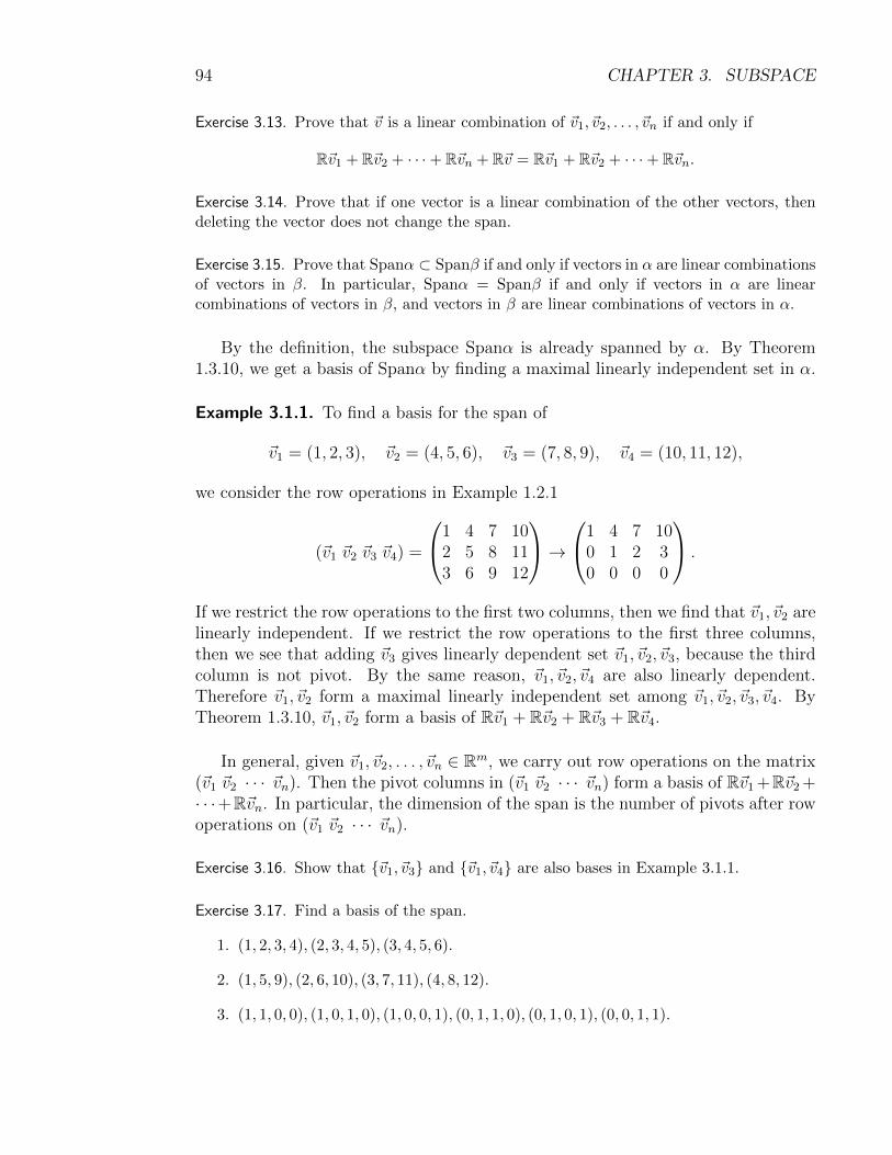
94 CHAPTER 3. SUBSPACE
Exercise 3.13. Prove that ~v is a linear combination of ~v1, ~v2, . . . , ~vn if and only if
R~v1 + R~v2 + · · ·+ R~vn + R~v = R~v1 + R~v2 + · · ·+ R~vn.
Exercise 3.14. Prove that if one vector is a linear combination of the other vectors, thendeleting the vector does not change the span.
Exercise 3.15. Prove that Spanα ⊂ Spanβ if and only if vectors in α are linear combinationsof vectors in β. In particular, Spanα = Spanβ if and only if vectors in α are linearcombinations of vectors in β, and vectors in β are linear combinations of vectors in α.
By the definition, the subspace Spanα is already spanned by α. By Theorem1.3.10, we get a basis of Spanα by finding a maximal linearly independent set in α.
Example 3.1.1. To find a basis for the span of
~v1 = (1, 2, 3), ~v2 = (4, 5, 6), ~v3 = (7, 8, 9), ~v4 = (10, 11, 12),
we consider the row operations in Example 1.2.1
(~v1 ~v2 ~v3 ~v4) =
1 4 7 102 5 8 113 6 9 12
→1 4 7 10
0 1 2 30 0 0 0
.
If we restrict the row operations to the first two columns, then we find that ~v1, ~v2 arelinearly independent. If we restrict the row operations to the first three columns,then we see that adding ~v3 gives linearly dependent set ~v1, ~v2, ~v3, because the thirdcolumn is not pivot. By the same reason, ~v1, ~v2, ~v4 are also linearly dependent.Therefore ~v1, ~v2 form a maximal linearly independent set among ~v1, ~v2, ~v3, ~v4. ByTheorem 1.3.10, ~v1, ~v2 form a basis of R~v1 + R~v2 + R~v3 + R~v4.
In general, given ~v1, ~v2, . . . , ~vn ∈ Rm, we carry out row operations on the matrix(~v1 ~v2 · · · ~vn). Then the pivot columns in (~v1 ~v2 · · · ~vn) form a basis of R~v1 +R~v2 +· · ·+R~vn. In particular, the dimension of the span is the number of pivots after rowoperations on (~v1 ~v2 · · · ~vn).
Exercise 3.16. Show that {~v1, ~v3} and {~v1, ~v4} are also bases in Example 3.1.1.
Exercise 3.17. Find a basis of the span.
1. (1, 2, 3, 4), (2, 3, 4, 5), (3, 4, 5, 6).
2. (1, 5, 9), (2, 6, 10), (3, 7, 11), (4, 8, 12).
3. (1, 1, 0, 0), (1, 0, 1, 0), (1, 0, 0, 1), (0, 1, 1, 0), (0, 1, 0, 1), (0, 0, 1, 1).

3.1. DEFINITION 95
4.
(1 10 0
),
(1 01 0
),
(1 00 1
),
(0 11 0
),
(0 10 1
),
(0 01 1
).
5. 1− t, t− t3, 1− t3, t3 − t5, t− t5.
By Exercise 1.32, the span has the following property.
Proposition 3.1.3. The following operations do not change the span.
1. {~v1, . . . , ~vi, . . . , ~vj, . . . , ~vn} → {~v1, . . . , ~vj, . . . , ~vi, . . . , ~vn}.
2. {~v1, . . . , ~vi, . . . , ~vn} → {~v1, . . . , c~vi, . . . , ~vn}, c 6= 0.
3. {~v1, . . . , ~vi, . . . , ~vj, . . . , ~vn} → {~v1, . . . , ~vi + c~vj, . . . , ~vj, . . . , ~vn}.
For vectors in a Euclidean space, the operations in Proposition 3.1.3 are columnoperations on the matrix (~v1 ~v2 · · · ~vn). The proposition basically says that columnoperations do not change the span. We can take advantage of the proposition tofind another way of calculating a basis of Spanα.
Example 3.1.2. For the four vectors in Example 3.1.1, we carry out column opera-tions on the matrix (~v1 ~v2 ~v3 ~v4)
1 4 7 102 5 8 113 6 9 12
C4−C3C3−C2C2−C1−−−−→
1 3 3 32 3 3 33 3 3 3
C4−C3C3−C2
13C2−−−−→
1 1 0 02 1 0 03 1 0 0
C1−C2C1↔C2−−−−→
1 0 0 01 1 0 01 2 0 0
.
The result is a column echelon form. By Proposition 3.1.3, we get
R~v1 + R~v2 + R~v3 + R~v4 = R(1, 1, 1) + R(0, 1, 2) + R(0, 0, 0) + R(0, 0, 0)
= R(1, 1, 1) + R(0, 1, 2).
The two pivot columns (1, 1, 1), (0, 1, 2) of the column echelon form are always lin-early independent, and therefore form a basis of R~v1 + R~v2 + R~v3 + R~v4.
Example 3.1.3. By taking the transpose of the row operation in Example 3.1.1, weget the column operation
1 2 34 5 67 8 910 11 12
→
1 0 04 −3 −67 −6 −1210 −9 −18
→
1 0 04 1 07 2 010 3 0
.
We find that (1, 4, 7, 10), (0, 1, 2, 3) form a basis of R(1, 4, 7, 10) + R(2, 5, 8, 11) +R(3, 6, 9, 12).

96 CHAPTER 3. SUBSPACE
In general, given ~v1, ~v2, . . . , ~vn ∈ Rm, we use column operations to find a columnechelon form of (~v1 ~v2 · · · ~vn). Then the pivot columns in the column echelon form(not the columns in the original matrix (~v1 ~v2 · · · ~vn)) is a basis of R~v1 + R~v2 +· · · + R~vn. In particular, the dimension of the span is the number of pivots aftercolumn operations on (~v1 ~v2 · · · ~vn). This is also the same as the number of pivotsafter row operations on the transpose (~v1 ~v2 · · · ~vn)T .
Comparing the dimension of the span obtained by two ways of calculating thespan, we conclude that applying row operations to A and AT give the same numberof pivots.
Exercise 3.18. Explain how Proposition 3.1.3 follows from Exercise 1.32.
Exercise 3.19. List all the 2× 3 column echelon forms.
Exercise 3.20. Explain that the nonzero columns in a column echelon form are linearlyindependent.
Exercise 3.21. Explain that, if the columns of an n × n matrix is a basis of Rn, then therows of the matrix is also a basis of Rn.
Exercise 3.22. Use column operations to find a basis of the span in Exercise 3.17.
3.1.3 Calculation of Extension to Basis
The column echelon form can also be used to extend linearly independent vectorsto a basis. By the proof of Theorem 1.3.11, this can be achieved by finding vectorsnot in the span.
Example 3.1.4. In Example 1.3.15, we use row operations to find that the vectors~v1 = (1, 4, 7, 11), ~v2 = (2, 5, 8, 12), ~v3 = (3, 6, 10, 10) in R4 are linearly independent.We may also use column operations to get
(~v1 ~v2 ~v3) =
1 2 34 5 67 8 1011 12 10
→
1 0 04 −3 −67 −6 −1111 −10 −23
→
1 0 04 −3 07 −6 111 −10 −3
.
This shows that (1, 4, 7, 11), (0,−3,−6,−10), (0, 0, 1,−3) form a basis of R~v1+R~v2+R~v3. In particular, the span has dimension 3. By Theorem 1.3.14, we find that~v1, ~v2, ~v3 are also linearly independent.
It is obvious that (1, 4, 7, 11), (0,−3,−6,−10), (0, 0, 1,−3), ~e4 = (0, 0, 0, 1) forma basis of R4. In fact, the same column operations (applied to the first three columns
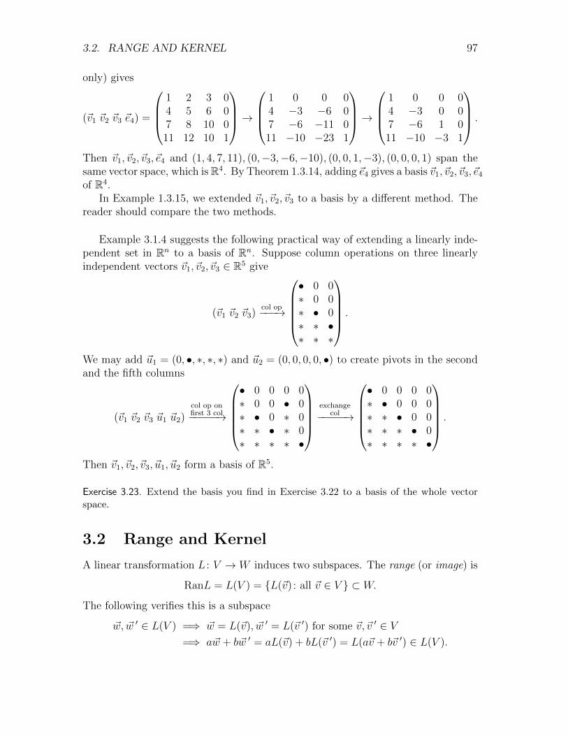
3.2. RANGE AND KERNEL 97
only) gives
(~v1 ~v2 ~v3 ~e4) =
1 2 3 04 5 6 07 8 10 011 12 10 1
→
1 0 0 04 −3 −6 07 −6 −11 011 −10 −23 1
→
1 0 0 04 −3 0 07 −6 1 011 −10 −3 1
.
Then ~v1, ~v2, ~v3, ~e4 and (1, 4, 7, 11), (0,−3,−6,−10), (0, 0, 1,−3), (0, 0, 0, 1) span thesame vector space, which is R4. By Theorem 1.3.14, adding ~e4 gives a basis ~v1, ~v2, ~v3, ~e4
of R4.In Example 1.3.15, we extended ~v1, ~v2, ~v3 to a basis by a different method. The
reader should compare the two methods.
Example 3.1.4 suggests the following practical way of extending a linearly inde-pendent set in Rn to a basis of Rn. Suppose column operations on three linearlyindependent vectors ~v1, ~v2, ~v3 ∈ R5 give
(~v1 ~v2 ~v3)col op−−−→
• 0 0∗ 0 0∗ • 0∗ ∗ •∗ ∗ ∗
.
We may add ~u1 = (0, •, ∗, ∗, ∗) and ~u2 = (0, 0, 0, 0, •) to create pivots in the secondand the fifth columns
(~v1 ~v2 ~v3 ~u1 ~u2)col op onfirst 3 col−−−−−→
• 0 0 0 0∗ 0 0 • 0∗ • 0 ∗ 0∗ ∗ • ∗ 0∗ ∗ ∗ ∗ •
exchange
col−−−−−→
• 0 0 0 0∗ • 0 0 0∗ ∗ • 0 0∗ ∗ ∗ • 0∗ ∗ ∗ ∗ •
.
Then ~v1, ~v2, ~v3, ~u1, ~u2 form a basis of R5.
Exercise 3.23. Extend the basis you find in Exercise 3.22 to a basis of the whole vectorspace.
3.2 Range and Kernel
A linear transformation L : V → W induces two subspaces. The range (or image) is
RanL = L(V ) = {L(~v) : all ~v ∈ V } ⊂ W.
The following verifies this is a subspace
~w, ~w ′ ∈ L(V ) =⇒ ~w = L(~v), ~w ′ = L(~v ′) for some ~v,~v ′ ∈ V=⇒ a~w + b~w ′ = aL(~v) + bL(~v ′) = L(a~v + b~v ′) ∈ L(V ).
98 CHAPTER 3. SUBSPACE
The kernel is the preimage of the zero vector
KerL = L−1(~0) = {~v : ~v ∈ V and L(~v) = ~0} ⊂ V.
The following verifies this is a subspace
~v,~v ′ ∈ KerL =⇒ L(~v) = ~0, L(~v ′) = ~0
=⇒ L(a~v + b~v ′) = aL(~v) + bL(~v ′) = a~0 + b~0 = ~0.
Exercise 3.24. Prove that Ran(L◦K) ⊂ RanL. Moreover, if K is onto, then Ran(L◦K) =RanL.
Exercise 3.25. Prove that Ker(L ◦K) ⊃ KerK. Moreover, if L is one-to-one, then Ker(L ◦K) = KerK.
Exercise 3.26. Suppose L : V → W is a linear transformation, and H ⊂ V is a subspace.Prove that L(H) = {L(~v) : all ~v ∈ H} is a subspace.
Exercise 3.27. Suppose L : V → W is a linear transformation, and H ⊂ W is a subspace.Prove that L−1(H) = {~v ∈ V : L(~v) ∈ H} is a subspace.
Exercise 3.28. Prove that L(H) ∩KerK = L(H ∩Ker(K ◦ L)).
3.2.1 Range
The range is actually defined for any map f : X → Y
Ranf = f(X) = {f(x) : all x ∈ X} ⊂ Y.
For the map Instructor: Courses → Professors, the range is all the professors whoteach some courses.
The map is onto if and only if f(X) = Y . This suggests that we may considerthe same map with smaller target
f : X → f(X), f(x) = f(x).
For the Instructor map, this means Instructor: Courses→ Teaching Professors. Theadvantage of the modification is the following.
Proposition 3.2.1. For any map f : X → Y , the corresponding map f : X → f(X)has the following properties.
1. f is onto.
2. f is one-to-one if and only if f is one-to-one.

3.2. RANGE AND KERNEL 99
Exercise 3.29. Prove Proposition 3.2.1.
Exercise 3.30. Prove that Ran(f ◦ g) ⊂ Ranf . Moreover, if g is onto, then Ran(f ◦ g) =Ranf .
Specialising to a linear transformation L : V → W , if α = {~v1, ~v2, . . . , ~vn} spansV , then any vector of V is a linear combination of α, and L is given by (2.1.1) forall vectors in V . This implies that the range subspace is a span
RanL = L(V ) = SpanL(α).
If L : Rn → Rm is actually a linear transformation of Euclidean spaces, with m× nmatrix A, then the interpretation above shows that the range of L is the span ofthe column vectors L(~ei) of A, called the column space
RanL = ColA ⊂ Rm.
Of course we can also consider the span of the rows of A and get the row space.The row and column spaces are clearly related by the transpose of the matrix
RowA = ColAT ⊂ Rn.
By Proposition 2.4.2 and the natural identification between (Rn)∗ and Rn in Example2.4.1, the row space corresponds to the range space of the dual linear transformationL∗.
Example 3.2.1. The derivative of a polynomial of degree n is a polynomial of degreen − 1. Therefore we have linear transformation D(f) = f ′ : Pn → Pm for m ≥ n − 1.By integrating polynomial (i.e., anti-derivative), we get RanD = Pn−1 ⊂ Pm. The lineartransformation is onto if and only if m = n− 1.
Example 3.2.2. Consider the linear transformation L(f) = f ′′ + (1 + t2)f ′ + tf : P3 → P4
in Example 2.3.3. The row operations in the earlier example shows that the following forma basis of RanL
L(1) = t, L(t) = 1 + 2t2, L(t2) = 2 + 2t+ 3t3, L(t3) = 6t+ 3t2 + 4t4.
Alternatively, we may carry out the column operations0 1 2 01 0 2 60 2 0 30 0 3 00 0 0 4
→
0 1 0 01 0 0 00 2 −4 30 0 3 00 0 0 4
→
0 1 0 01 0 0 00 2 −4 00 0 3 9
40 0 0 4
→
1 0 0 00 1 0 02 0 −4 00 0 3 90 0 0 16
.
This shows that 1 + 2t2, t,−4t2 + 3t3, 9t3 + 16t4 form a basis of RanL. It is also easy tosee that adding t4 gives a basis of P4.

100 CHAPTER 3. SUBSPACE
Example 3.2.3. Consider the linear transformation L(A) = A+AT : Mn×n →Mn×n. By(A+AT )T = AT +(AT )T = AT +A = A+AT , any X = A+AT ∈ RanL satisfies XT = X.Such matrices are called symmetric because they are of the form (for n = 3, for example)
X =
a11 a12 a13
a12 a22 a23
a13 a23 a33
=
a d ed b fe f c
.
Conversely, if X = XT , then for A = 12X, we have
L(A) = A+AT =1
2X +
1
2XT =
1
2X +
1
2X = X.
This shows that any symmetric matrix lies in RanL. Therefore the range of L consists ofexactly all the symmetric matrices. A basis of 3× 3 symmetric matrices is given bya d e
d b fe f c
= a
1 0 00 0 00 0 0
+ b
0 0 00 1 00 0 0
+ c
0 0 00 0 00 0 1
+ d
0 1 01 0 00 0 0
+ e
0 0 10 0 01 0 0
+ f
0 0 00 0 10 1 0
.
Exercise 3.31. Explain that A~x = ~b has solution if and only if ~b ∈ ColA.
Exercise 3.32. Suppose L : V →W is a linear transformation.
1. Prove the modified linear transformation (see Proposition 3.2.1) L : V → L(V ) isan onto linear transformation.
2. Let i : L(V )→W be the inclusion linear transformation in Exercise 3.9. Show thatL = i ◦ L.
Exercise 3.33. Suppose L : V → W is a linear transformation. Prove that L is one-to-oneif and only if L : V → L(V ) is an isomorphism.
Exercise 3.34. Show that the range of the linear transformation L(A) = A−AT : Mn×n →Mn×n consists of matrices X satisfying XT = −X. These are called skew-symmetricmatrices.
Exercise 3.35. Find the dimensions of the subspaces of symmetric and skew-symmetricmatrices.
3.2.2 Rank
The span of a set of vectors, the range of a linear transformation, and the columnspace of a matrix are different presentations of the same concept. Their size, which
3.2. RANGE AND KERNEL 101
is their dimension, is the rank
rankα = dim Spanα, rankL = dim RanL, rankA = dim ColA.
By the calculation of basis of span subspace in Section 3.1.1, the rank of a matrixA is the number of pivots in the row echelon form, and is also the number of pivots inthe column echelon form. Since column operation on A is the same as row operationon AT , we have
rankAT = rankA.
By Proposition 2.4.2, this means
rankL∗ = rankL.
Since the number of pivots of an m×n matrix is always no more than m and n,we have
rankAm×n ≤ min{m,n}.
If the equality holds, then the matrix has full rank. This means either rankAm×n = m(all rows are pivot), or rankAm×n = n (all columns are pivot). By Propositions 1.3.4,1.3.6, 2.2.9, we have the following.
Proposition 3.2.2. Let A be an m×n matrix. Then rankA ≤ min{m,n}. Moreover,
1. A~x = ~b has solution for all ~b if and only if rankA = m.
2. The solution of A~x = ~b is unique if and only if rankA = n.
3. A is invertible if and only if rankA = m = n.
The following is the same result for set of vectors. The first statement actu-ally follows from Proposition 3.1.2, and the second statement may be obtained byapplying Theorem 1.3.14 to V = Spanα.
Proposition 3.2.3. Let α be a set of n vectors in V . Then rankα ≤ min{n, dimV },Moreover,
1. α spans V if and only if rankα = dimV .
2. α is linearly independent if rankα = n.
3. α is a basis of V if and only if rankα = dimV = n.
The following is the same result for linear transformation. The first statementactually follows from Proposition 3.1.2, and the second statement may be obtainedby applying Theorem 2.2.6 to L : V → RanL in Exercises 3.32 and 3.33.
102 CHAPTER 3. SUBSPACE
Proposition 3.2.4. Let L : V → W be a linear transformation. Then rankL ≤min{dimV, dimW}. Moreover,
1. L is onto if and only if rankL = dimW .
2. L is one-to-one if and only if rankL = dimV .
3. L is invertible if and only if rankL = dimV = dimW .
Exercise 3.36. What is the rank of the vector set in Exercise 3.17?
Exercise 3.37. If a set of vectors is enlarged, how is the rank changed?
Exercise 3.38. Suppose the columns of an m×n matrix A are linearly independent. Provethat there are n rows of A that are also linearly independent. Similarly, if the rows of Aare linearly independent, then there are n columns of A that are also linearly independent.
Exercise 3.39. Directly prove Proposition 3.2.3.
Exercise 3.40. Consider a composition UK−→ V
L−→ W . Let L|K(U) : K(U) → W be therestriction of L to the subspace K(U).
1. Prove Ran(L ◦K) = RanL|K(U) ⊂ RanL.
2. Prove rank(L ◦K) ≤ min{rankL, rankK}.
3. Prove rank(L ◦K) = rankL when K is onto.
4. Prove rank(L ◦K) = rankK when L is one-to-one.
5. Translate the second part into a fact about matrices.
3.2.3 Kernel
By the third part of Proposition 2.2.4, we know that a linear transformation L isone-to-one if and only if KerL = {~0}. In contrast, the linear transformation is ontoif and only if RanL is the whole target space.
For a linear transformation L(~x) = A~x : Rn → Rm between Euclidean spaces,the kernel is all the solutions of the homogeneous system of linear equations, calledthe null space
NulA = KerL = {~v : all ~v ∈ Rn satisfying A~v = ~0}.
The uniqueness of solution means NulA = {~0}. In contrast, the existence of solution(for all right side) means ColA = Rm.

3.2. RANGE AND KERNEL 103
Example 3.2.4. To find the null space of
A =
1 4 7 102 5 8 113 6 9 12
,
we use the row operation in Example 1.2.1 and continue to get the reduced rowechelon form
A −→
1 4 7 100 1 2 30 0 0 0
−→1 0 −1 −2
0 1 2 30 0 0 0
As pointed out in Section 1.2.4, this is the same as the general solution of thehomogeneous system A~x = ~0. We express the solution in vector form
~x =
x1
x2
x3
x4
=
x3 + 2x4
−2x3 − 3x4
x3
x4
= x3
1−210
+ x4
2−301
= x3~v1 + x4~v2.
Since the free variables x3, x4 can be arbitrary, this shows that NulA = R~v1 + R~v2.The following further shows that ~v1, ~v2 are linearly independent
x3~v1 + x4~v2 = ~0 ⇐⇒ the solution ~x = ~0
=⇒ coordinates of the solution x3 = x4 = 0.
In general, the solution of a homogeneous system A~x = ~0 is ~x = c1~v1 + c2~v2 +· · ·+ ck~vk, where c1, c2, . . . , ck are all the free variables. This implies NulA = R~v1 +R~v2 + · · ·+R~vk. Moreover, the argument in the example shows that the vectors arealways linearly independent. Therefore ~v1, ~v2, . . . , ~vk form a basis of NulA.
The nullity dim NulA of a matrix is the dimension of the null space. The calcu-lation of the null space shows that the nullity is the number of non-pivot columns(corresponding to free variables) of A. Since rankA = dim ColA is the number ofpivot columns (corresponding to non-free variables) of A, we conclude that
dim NulA+ rankA = number of columns of A.
Translated into linear transformations, this means the following.
Theorem 3.2.5. If L : V → W is a linear transformation, then dim KerL+rankL =dimV .
Example 3.2.5. For the linear transformation L(f) = f ′′ : P5 → P3, we have
KerL = {f ∈ P5 : f ′′ = 0} = {a+ bt : a, b ∈ R}.

104 CHAPTER 3. SUBSPACE
The monomials 1, t form a basis of the kernel, and dim KerL = 2. Since L(P5) = P3
is onto, we have rankL = dimL(P5) = dimP3 = 4. Then
dim KerL+ rankL = 2 + 4 = 6 = dimP5.
This confirms Theorem 3.2.5.
Example 3.2.6. Consider the linear transformation
L(f) = (1 + t2)f ′′ + (1 + t)f ′ − f : P3 → P3
in Examples 2.1.16 and 2.3.3. The row operations in Example 2.3.3 show thatrankL = 3. Therefore dim KerL = dimP3 − rankL = 1. Since we already knowL(1 + t) = 0, we conclude that KerL = R(1 + t).
Example 3.2.7. By Exercise 2.20, the left multiplication by an m × n matrix A isa linear transformation
LA(X) = AX : Mn×k →Mm×k.
Let X = (~x1 ~x2 · · · ~xk). Then AX = (A~x1 A~x2 · · · A~xk). Therefore Y ∈ RanLA ifand only if all columns of Y lie in ColA, and X ∈ KerLA if and only if all columnsof X lie in NulA.
Let α = {~v1, ~v2, . . . , ~vr} be a basis of ColA (r = rankA). Then for the specialcase k = 2, the following is a basis of RanLA
(~v1~0), (~0 ~v1), (~v2
~0), (~0 ~v2), . . . , (~vr ~0), (~0 ~vr).
Therefore dim RanLA = 2r = 2 dim ColA. Similarly, we have dim KerLA = 2r =2 dim NulA.
In general, we have
dim RanLA = k dim ColA = k rankA,
dim KerLA = k dim NulA = k(n− rankA).
Example 3.2.8. In Example 3.2.3, we saw the range of linear transformation L(A) =A+ AT : Mn×n → Mn×n is exactly all symmetric matrices. The kernel of the lineartransformation consists those A satisfying A+AT = O, or AT = −A. These are theskew-symmetric matrices. See Exercises 3.34 and 3.35. We have
rankL = dim{symmetric matrices}
= 1 + 2 + · · ·+ n =1
2n(n+ 1),
and
dim{skew-symmetric matrices} = dimMn×n − rankL
= n2 − 1
2n(n+ 1) =
1
2n(n− 1).

3.2. RANGE AND KERNEL 105
Exercise 3.41. Use Theorem 3.2.5 to show that L : V → W is one-to-one if and only ifrankL = dimV (the second statement of Proposition 3.2.4).
Exercise 3.42. An m× n matrix A induces four subspaces ColA,RowA,NulA,NulAT .
1. Which are subspaces of Rm? Which are subspaces of Rn?
2. Which basis can you calculate by using row operations on A?
3. Which basis can you calculate by using column operations on A?
4. What are the dimensions in terms of the rank of A?
Exercise 3.43. Find a basis of the kernel of the linear transformation given by the matrix(some appeared in Exercise 1.28).
1.
1 2 3 43 4 5 65 6 7 87 8 9 10
.
2.
1 3 5 72 4 6 83 5 7 94 6 8 10
.
3.
1 2 32 3 43 4 14 1 2
.
4.
1 2 3 42 3 4 13 4 1 2
.
5.
1 2 3 12 3 1 23 1 2 3
.
6.
1 2 32 3 13 1 21 2 3
.
Exercise 3.44. Find the rank and nullity.
1. L(x1, x2, x3, x4) = (x1 + x2, x2 + x3, x3 + x4, x4 + x1).
2. L(x1, x2, x3, x4) = (x1 + x2 + x3, x2 + x3 + x4, x3 + x4 + x1, x4 + x1 + x2).
3. L(x1, x2, x3, x4) = (x1 − x2, x1 − x3, x1 − x4, x2 − x3, x2 − x4, x3 − x4).
4. L(x1, x2, . . . , xn) = (xi − xj)1≤i<j≤n.
5. L(x1, x2, . . . , xn) = (xi + xj)1≤i<j≤n.
Exercise 3.45. Find the rank and nullity.
1. L(f) = f ′′ + (1 + t2)f ′ + tf : P3 → P4.
2. L(f) = f ′′ + (1 + t2)f ′ + tf : P3 → P5.
3. L(f) = f ′′ + (1 + t2)f ′ + tf : Pn → Pn+1.
Exercise 3.46. Find the dimensions of the range and the kernel of right multiplication byan m× n matrix A
RA(X) = XA : Mk×m →Mk×n.
106 CHAPTER 3. SUBSPACE
3.2.4 General Solution of Linear Equation
Let L : V → W be a linear transformation, and ~b ∈ W . Then L(~x) = ~b has solution
(i.e., there is ~x0 ∈ V satisfying the equation) if and only if ~b ∈ RanL. Next, we try
to find the collection of all solutions (i.e., the preimage of ~b)
L−1(~b) = {~x ∈ V : L(~x) = ~b}.
ByL(~x) = ~b ⇐⇒ L(~x− ~x0) = ~b−~b = ~0 ⇐⇒ ~x− ~x0 ∈ KerL,
we conclude that
L−1(~b) = ~x0 + KerL = {~x0 + ~v : L(~v) = ~0}.
In terms of system of linear equations, this means that the solution of A~x = ~b (in
case ~b ∈ ColA) is of the form ~x0 +~v, where ~x0 is one special solution, and ~v ∈ NulAis any solution of the homogeneous system A~x = ~0.
Geometrically, the kernel is a subspace. The collection of all solutions is obtainedby shifting the subspace by one special solution ~x0.
We note the range (and ~x0) manifests the existence, while the kernel manifeststhe variations in the solution. In particular, the uniqueness of solution means novariation, or the triviality of the kernel.
Example 3.2.9. The system of linear equations
x1 + 4x2 + 7x3 + 10x4 = 1,
2x1 + 5x2 + 8x3 + 11x4 = 1,
3x1 + 6x2 + 9x3 + 12x4 = 1,
has an obvious solution ~x0 = 13(−1, 1, 0, 0). In Example 3.2.4, we found that ~v1 =
(1,−2, 1, 0) and ~v2 = (2,−3, 0, 1) form a basis of the kernel. Therefore the generalsolution is (c1, c2 are arbitrary)
~x = ~x0 + c1~v1 + c2~v2 =1
3
−1100
+ c1
1−210
+ c2
2−301
=
−1
3+ c1 + 2c2
13− 2c1 − 3c2
c1
c2
.
Geometrically, the solutions is the plane R(1,−2, 1, 0) + R(1,−2, 1, 0) shifted by~x0 = 1
3(−1, 1, 0, 0).
We may also use another obvious solution 13(0,−1, 1, 0) and get an alternative
formula for the general solution
~x =1
3
0−110
+ c1
1−210
+ c2
2−301
=
c1 + 2c2
−13− 2c1 − 3c2
13
+ c1
c2
.
3.2. RANGE AND KERNEL 107
Example 3.2.10. For the linear transformation in Examples 2.1.16 and 2.3.3
L(f) = (1 + t2)f ′′ + (1 + t)f ′ − f : P3 → P3,
we know from Example 3.2.6 that the kernel is R(1+t). Moreover, by L(1), L(t2), L(t3)in Example 2.3.3, we also know L(2 − t2 + t3) = 4t + 8t3. Therefore 1
4(2 − t2 + t3)
is a special solution of the differential equation in Example 2.1.16. Then we get thegeneral solution in Example 2.3.3
f = 14(2− t2 + t3) + c(1 + t).
Example 3.2.11. The general solution of the linear differential equation f ′ = sin tis
f = − cos t+ C.
Here f0 = − cos t is one special solution, and the arbitrary constants C form thekernel of the derivative linear transform
Ker(f 7→ f ′) = {C : C ∈ R} = R1.
Similarly, f ′′ = sin t has a special solution f0 = − sin t. Moreover, we have (seeExample 3.2.5)
Ker(f 7→ f ′′) = {C +Dt : C,D ∈ R} = R1 + Rt.
Therefore the general solution of f ′′ = sin t is f = − sin t+ C +Dt.
Example 3.2.12. The left side of a linear differential equation of order n (see Ex-ample 2.1.15)
L(f) =dnf
dtn+ a1(t)
dn−1f
dtn−1+ a2(t)
dn−2f
dtn−2+ · · ·+ an−1(t)
df
dt+ an(t)f = b(t)
is a linear transformation C∞ → C∞. A fundamental theorem in the theory ofdifferential equations says that dim KerL = n. Therefore to solve the differentialequation, we need to find one special function f0 satisfying L(f0) = b(t) and nlinearly independent functions f1, f2, . . . , fn satisfying L(fi) = 0. Then the generalsolution is
f = f0 + c1f1 + c2f2 + · · ·+ cnfn.
Take the second order differential equation f ′′+f = et as an example. We try thespecial solution f0 = aet and find (aet)′′+aet = 2aet = et implying a = 1
2. Therefore
f0 = 12et is a solution. Moreover, we know that both f1 = cos t and f2 = sin t satisfy
the homogeneous equation f ′′ + f = 0. By Example 1.3.11, f1 and f2 are linearlyindependent. This leads to the general solution of the differential equation
f = 12et + c1 cos t+ c2 sin t, c1, c2 ∈ R.
Exercise 3.47. Find a basis of the kernel of L(f) = f ′′+ 3f ′−4f by trying functions of theform f(t) = eat. Then find general solution.

108 CHAPTER 3. SUBSPACE
1. f ′′ + 3f ′ − 4f = 1 + t.
2. f ′′ + 3f ′ − 4f = et.
3. f ′′ + 3f ′ − 4f = cos t+ 2 sin t.
4. f ′′ + 3f ′ − 4f = 1 + t+ et.
3.3 Sum of Subspace
The sum of subspaces generalises the span. The direct sum of subspaces generalisesthe linear independence. Subspace, sum, and direct sum are the deeper linear algebraconcepts that replace vector, span, and linear independence.
3.3.1 Sum and Direct Sum
Definition 3.3.1. The sum of subspaces H1, H2, . . . , Hk ⊂ V is
H1 +H2 + · · ·+Hk = {~h1 + ~h2 + · · ·+ ~hk : ~hi ∈ Hi}.
The sum is direct if
~h1 + ~h2 + · · ·+ ~hk = ~h′1 + ~h′2 + · · ·+ ~h′k,~hi,~h
′i ∈ Hi =⇒ ~hi = ~h′i.
We indicate the direct sum by writing H1 ⊕H2 ⊕ · · · ⊕Hk.
If Hi = R~vi, then the sum is the span of α = {~v1, ~v2, . . . , ~vk}. If ~vi 6= ~0, then thedirect sum means that α is linearly independent.
Example 3.3.1. Let P evenn be all the even polynomials in Pn and P odd
n be all the oddpolynomials in Pn. Then Pn = P even
n ⊕ P oddn .
Example 3.3.2. For k = 1, we have the sum H1 of single vector space H1. Thesingle sum is always direct.
For H1 +H2 to be direct, we require
~h1 + ~h2 = ~h′1 + ~h′2 =⇒ ~h1 = ~h′1,~h2 = ~h′2.
Let ~v1 = ~h1 − ~h′1 ∈ H1 and ~v2 = ~h2 − ~h′2 ∈ H2. Then the condition becomes
~v1 + ~v2 = ~0 =⇒ ~v1 = ~v2 = ~0.
The equality on the left means ~v1 = −~v2, which is a vector in H1 ∩H2. Thereforethe condition above means exactly H1 ∩H2 = {~0}. This is the criterion for the sumH1 +H2 to be direct.
Example 3.3.3 (Abstract Direct Sum). Let V and W be vector spaces. Construct avector space V ⊕W to be the set V ×W = {(~v, ~w) : ~v ∈ V, ~w ∈ W}, together withaddition and scalar multiplication
(~v1, ~w1) + (~v2, ~w2) = (~v1 + ~v2, ~w1 + ~w2), a(~v, ~w) = (a~v, a~w).

3.3. SUM OF SUBSPACE 109
It is easy to verify that V ⊕W is a vector space. Moreover, V and W are isomorphicto the following subspaces of V ⊕W
V ∼= V ⊕~0 = {(~v,~0W ) : ~v ∈ V }, W ∼= ~0⊕W = {(~0V , ~w) : ~w ∈ W}.
Since any vector in V ⊕W can be uniquely expressed as (~v, ~w) = (~v,~0W ) + (~0V , ~w),we find that V ⊕W is the direct sum of two subspaces
V ⊕W = {(~v,~0W ) : ~v ∈ V } ⊕ {(~0V , ~w) : ~w ∈ W}.
This is the reason why V ⊕W is called abstract direct sum.The construction allows us to write Rm ⊕ Rn = Rm+n. Strictly speaking, Rm
and Rn are not subspaces of Rm+n. The equality means
1. Rm is isomorphic to the subspace of vectors in Rm+n with the last n coordinatesvanishing.
2. Rn is isomorphic to the subspace of vectors in Rm+n with the first m coordi-nates vanishing.
3. Rm+n is the direct sum of these two subspaces.
Exercise 3.48. Prove that
H1 +H2 = H2 +H1, (H1 +H2) +H3 = H1 +H2 +H3 = H1 + (H2 +H3).
Exercise 3.49. Prove that an intersection H1 ∩H2 ∩ · · · ∩Hk of subspaces is a subspace.
Exercise 3.50. Prove that H1 +H2 + · · ·+Hk is the smallest subspace containing all Hi.
Exercise 3.51. Prove that Spanα+ Spanβ = Span(α ∪ β).
Exercise 3.52. Prove that Span(α∩β) ⊂ (Spanα)∩ (Spanβ). Show that the two sides mayor may not equal.
Exercise 3.53. We may regard a subspace H as a sum of single subspace. Explain that thesingle sum is always direct.
Exercise 3.54. If a sum is direct, prove that the sum of a selection of subspaces is alsodirect.
Exercise 3.55. Prove that a sum H1+H2+· · ·+Hk is direct if and only if the sum expressionfor ~0 is unique
~h1 + ~h2 + · · ·+ ~hk = ~0, ~hi ∈ Hi =⇒ ~h1 = ~h2 = · · · = ~hk = ~0.
The generalises Proposition 1.3.7.
110 CHAPTER 3. SUBSPACE
Exercise 3.56. Prove that a sum H1 +H2 + · · ·+Hk is direct if and only if
~h1 + ~h2 + · · ·+ ~hk−1 ∈ Hk, ~hi ∈ Hi =⇒ ~h1 = ~h2 = · · · = ~hk−1 = ~0.
Explain that this generalises Proposition 1.3.8.
Exercise 3.57. Show that Mn×n is the direct sum of the subspace of symmetric matrices(see Example 3.2.3) and the subspace of skew-symmetric matrices (see Exercise 3.34). Inother words, any square matrix is the sum of a unique symmetric matrix and a uniqueskew-symmetric matrix.
Exercise 3.58. Let H,H ′ be subspaces of V . We have the sum H + H ′ ⊂ V and wealso have the abstract direct sum H ⊕ H ′ from Example 3.3.3. Prove that L(~h,~h′) =~h + ~h′ : H ⊕ H ′ → H + H ′ is an onto linear transformation, and KerL is isomorphic toH ∩H ′.
Exercise 3.59. Use Exercise 3.58 to prove dim(H +H ′) = dimH + dimH ′ − dim(H ∩H ′).
In general, a sum of sums of subspaces is a sum. For example, we have
(H1 +H2) +H3 + (H4 +H5) = H1 +H2 +H3 +H4 +H5.
We will show that the sum on the right is direct if and only if H1 +H2, H3, H4 +H5,(H1 +H2) +H3 + (H4 +H5) are direct sums.
To state the general result, we consider n sums
Hi = +jHij = +kij=1Hij = Hi1 +Hi2 + · · ·+Hiki , i = 1, 2, . . . , n.
Then we consider the sum
H = +i(+jHij) = +ni=1Hi = H1 +H2 + · · ·+Hn,
and consider the further splitting of the sum
H = +ijHij = H11 +H12 + · · ·+H1k1 +H21 +H22 + · · ·+H2k2
+ · · · · · ·+Hn1 +Hn2 + · · ·+Hnkn .
Proposition 3.3.2. The sum +ijHij is direct if and only if the sum +i(+jHij) isdirect and the sum +jHij is direct for each i.
Proof. Suppose H = +ijHij is a direct sum. To prove that H = +iHi = +i(+jHij)
is direct, we consider a vector ~h =∑
i~hi = ~h1 + ~h2 + · · ·+ ~hn, ~hi ∈ Hi, in the sum.
By Hi = +jHij, we have ~hi =∑
j~hij = ~hi1 + ~hi2 + · · · + ~hiki ,
~hij ∈ Hij. Then~h =
∑ij~hij. Since H = +ijHij is direct, we find that ~hij are uniquely determined

3.3. SUM OF SUBSPACE 111
by ~h. This implies that ~hi are also uniquely determined by ~h. This proves thatH = +iHi is direct.
Next we further prove that Hi = +jHij is also direct. We consider a vector~h =
∑j~hij = ~hi1 + ~hi2 + · · · + ~hiki ,
~hij ∈ Hij, in the sum. By taking ~hi′j = ~0 for
all i′ 6= i, we form the double sum ~h =∑
ij~hij. Since H = +ijHij is direct, all ~hpj,
p = i or p = i′, are uniquely determined by ~h. In particular, ~hi1,~hi2, . . . ,~hiki are
uniquely determined by ~h. This proves that Hi = +jHij is direct.Conversely, suppose the sum +i(+jHij) is direct and the sum +jHij is direct
for each i. To prove that H = +ijHij is direct, we consider a vector ~h =∑
ij~hij,
~hij ∈ Hij, in the sum. We have ~h =∑
i~hi for ~hi =
∑j~hij ∈ +jHij. Since
H = +i(+jHij) is direct, we find that ~hi are uniquely determined by ~h. Since
Hi = +jHij is direct, we also find that ~hij are uniquely determined by ~hi. Therefore
all ~hij are uniquely determined by ~h. This proves that +ijHij is direct.
For the special case Hij = R~vij is spanned by a single non-zero vector, theequality +i(+jHij) = +ijHij means that, if αi = {~vi1, ~vi2, . . . , ~viki} spans Hi foreach i, then the union α = α1 ∪ α2 ∪ · · · ∪ αk = {~vij : all i, j} spans the sumH = H1 + H2 + · · · + Hk. If αi is a basis of Hi, then by Propositions 1.3.13, 3.3.2and Theorem 1.3.14, we get the following.
Proposition 3.3.3. If H1, H2, . . . , Hk are finite dimensional subspaces, then
dim(H1 +H2 + · · ·+Hk) ≤ dimH1 + dimH2 + · · ·+ dimHk.
Moreover, the sum is direct if and only if the equality holds.
Exercise 3.60. Suppose αi are linearly independent. Prove that the sum Spanα1+Spanα2+· · ·+ Spanαk is direct if and only if α1 ∪ α2 ∪ · · · ∪ αk is linearly independent.
Exercise 3.61. Suppose αi is a basis of Hi. Prove that α1 ∪ α2 ∪ · · · ∪ αk is a basis ofH1 +H2 + · · ·+Hk if and only if the sum H1 +H2 + · · ·+Hk is direct.
3.3.2 Projection
A direct sum V = H ⊕ H ′ induces a map by picking the first term in the uniqueexpression
P (~v) = ~h, if ~v = ~h+ ~h′, ~h ∈ H, ~h′ ∈ H ′.
The direct sum implies that P is a well defined linear transformation satisfyingP 2 = P . See Exercise 3.62.
Definition 3.3.4. A linear operator P : V → V is a projection if P 2 = P .

112 CHAPTER 3. SUBSPACE
Conversely, given any projection P , we have ~v = P (~v) + (I − P )(~v). By P (I −P )(~v) = (P −P 2)(~v) = ~0, we have P (~v) ∈ RanP and (I −P )(~v) ∈ KerP . Therefore
V = RanP +KerP . On the other hand, if ~v = ~h+~h′ with ~h ∈ RanP and ~h′ ∈ KerP ,then ~h = P (~w) for some ~w ∈ V , and
P (~v) = P (~h) + P (~h′)
= P (~h) (~h′ ∈ KerP )
= P 2(~w) (~h = P (~w))
= P (~w) (P 2 = P )
= ~h.
This shows that ~h is unique. Therefore the decomposition ~v = ~h+~h′ is also unique,and we have a direct sum
V = RanP ⊕KerP.
We conclude that there is a one-to-one correspondence between projections of Vand decompositions of V into direct sums of two subspaces.
Example 3.3.4. With respect to the direct sum Pn = P evenn ⊕P odd
n in Example 3.3.1,the projection to even polynomials is given by f(t) 7→ 1
2(f(t) + f(−t)).
Example 3.3.5. In C∞, we consider subspaces
H = R1 = {constant functions}, H ′ = {f : f(0) = 0}.
Since any function f(t) = f(0) + (f(t)− f(0)) with f(0) ∈ H and f(t)− f(0) ∈ H ′,we have C∞ = H +H ′. Since H ∩H ′ consists of zero function only, we have directsum C∞ = H⊕H ′. Moreover, the projection to H is f(t) 7→ f(0) and the projectionto H ′ is f(t) 7→ f(t)− f(0).
Exercise 3.62. Given a direct sum V = H ⊕H ′, verify that P (~v) = ~h is well defined, is alinear operator, and satisfies P 2 = P .
Exercise 3.63. Directly verify that the matrix A of the orthogonal projection in Example2.1.13 satisfies A2 = A.
Exercise 3.64. For the orthogonal projection P in Example 2.1.13, explain that I − P isalso a projection. What is the subspace corresponding to I − P?
Exercise 3.65. If P is a projection, prove that Q = I − P is also a projection satisfying
P +Q = I, PQ = QP = O.

3.3. SUM OF SUBSPACE 113
Moreover, P and Q induce the same direct sum decomposition
V = H ⊕H ′, H = RanP = KerQ, H ′ = RanQ = KerP,
with the only exception that the order of H and H ′ are switched.
Exercise 3.66. Find the formula for the projections given by the direct sum in Exercise3.57
Mn×n = {symmetric matrix} ⊕ {skew-symmetric matrix}.
Exercise 3.67. Consider subspaces in C∞
H = R1⊕ Rt = {polynomials of degree ≤ 1}, H ′ = {f : f(0) = f(1) = 0}.
Show that we have a direct sum C∞ = H ⊕H ′, and find the corresponding projections.Moreover, generalise to higher order polynomials and evaluation at more points (and notnecessarily including 0 or 1).
Suppose we have a direct sum
V = H1 ⊕H2 ⊕ · · · ⊕Hk.
Then the direct sum V = Hi⊕ (⊕j 6=iHj) corresponds to a projection Pi : V → Hi ⊂V . It is easy to see that the unique decomposition
~v = ~h1 + ~h2 + · · ·+ ~hk, ~hi ∈ Hi,
gives (and is given by) ~hi = Pi(~v). The interpretation immediately implies
P1 + P2 + · · ·+ Pk = I, PiPj = O for i 6= j.
Conversely, given linear operators Pi satisfying the above, we get Pi = PiI = PiP1 +PiP2 + · · ·+ PiPk = P 2
i . Therefore Pi is a projection. Moreover, if
~v = ~h1 + ~h2 + · · ·+ ~hk, ~hi = Pi(~wi) ∈ Hi = RanPi,
then
Pi(~v) = PiP1(~w1) + PiP2(~w2) + · · ·+ PiPk(~wk) = P 2i (~wi) = Pi(~wi) = ~hi.
This implies the uniqueness of ~hi, and we get a direct sum.
Proposition 3.3.5. There is a one-to-one correspondence between direct sum de-compositions of a vector space V and collections of projections Pi satisfying
P1 + P2 + · · ·+ Pk = I, PiPj = O for i 6= j.

114 CHAPTER 3. SUBSPACE
Example 3.3.6. The basis in Examples 1.3.17 and 2.1.13
~v1 = (1,−1, 0), ~v2 = (1, 0,−1), ~v3 = (1, 1, 1),
gives a direct sum R3 = R~v1⊕R~v2⊕R~v3. Then we have three projections P1, P2, P3
corresponding to three 1-dimensional subspaces
~b = x1~v1 + x2~v2 + x3~v3 =⇒ P1(~b) = x1~v1, P2(~b) = x2~v2, P3(~b) = x3~v3.
The calculation of the projections becomes the calculation of the formulae of x1, x2, x3
in terms of ~b. In other words, we need to solve the equation A~x = ~b for the matrixA in Example 2.2.18. The solution isx1
x2
x3
= A−1~b =1
3
1 −2 11 1 −21 1 1
b1
b2
b3
.
Therefore
P1(~b) = 13(b1 − 2b2 + b3)(1,−1, 0),
P2(~b) = 13(b1 + b2 − 2b3)(1, 0,−1),
P3(~b) = 13(b1 + b2 + b3)(1, 1, 1).
The matrices of the projections are
[P1] = 13
1 −2 1−1 2 −10 0 0
, [P2] = 13
1 1 −20 0 0−1 −1 2
, [P3] = 13
1 1 11 1 11 1 1
.
We also note that the projection to the subspace R~v1 ⊕ R~v2 in the direct sumR3 = R~v1 ⊕ R~v2 ⊕ R~v3 is P1 + P2 (see Exercise 3.68)
~b = (x1~v1 + x2~v2) + x3~v3 7→ x1~v1 + x2~v2 = P1(~b) + P2(~b).
The matrix of the projection is [P1] + [P2], which can also be calculated as follows
[P1] + [P2] = I − [P3] = 13
2 −1 −1−1 2 −1−1 −1 2
.
Exercise 3.68. Suppose the direct sum V = H1 ⊕H2 ⊕H3 corresponds to the projectionsP1, P2, P3. Prove that the projection to H1 ⊕H2 in the direct sum V = (H1 ⊕H2) ⊕H3
is P1 + P2.
Exercise 3.69. For the direct sum given by the basis in Example 2.2.17
R3 = R(1, 2, 3)⊕ R(4, 5, 6)⊕ R(7, 8, 10),
find the projections to the three lines. Then find the projection to the plane R(1, 2, 3) ⊕R(4, 5, 6).
3.3. SUM OF SUBSPACE 115
Exercise 3.70. For the direct sum given by modifying the basis in Example 2.1.13
R3 = R(1,−1, 0)⊕ R(1, 0,−1)⊕ R(1, 0, 0),
find the projection to the plane R(1,−1, 0)⊕ R(1, 0,−1).
Exercise 3.71. In Example 3.1.4, a set of linearly independent vectors ~v1, ~v2, ~v3 is extendedto a basis by adding ~e4 = (0, 0, 0, 1). Find the projections related to the direct sumR4 = Span{~v1, ~v2, ~v3} ⊕ R~e4.
Exercise 3.72. We know the rank of
A =
1 4 7 102 5 8 113 6 9 12
is 2, and A~e1, A~e2 are linearly independent. Show that we have a direct sum R4 =NulA⊕ Span{~e1, ~e2}. Moreover, find the projections corresponding to the direct sum.
Exercise 3.73. The basis t(t − 1), t(t − 2), (t − 1)(t − 2) in Example 1.3.12 gives a directsum P2 = Span{t(t− 1), t(t− 2)} ⊕ R(t− 1)(t− 2). Find the corresponding projections.
3.3.3 Blocks of Linear Transformation
Suppose L : V → W is a linear transformation. Suppose α = {~v1, ~v2, ~v3} and β ={~w1, ~w2} are bases of V and W . Then the matrix of
L : V = R~v1 ⊕ R~v2 ⊕ R~v3 → W = R~w1 ⊕ R~w2
means
[L]βα =
(a11 a12 a13
a21 a22 a23
),
L(~v1) = a11 ~w1 + a21 ~w2,
L(~v2) = a12 ~w1 + a22 ~w2,
L(~v3) = a13 ~w1 + a23 ~w2.
Let P1 : W → W be the projection to R~w1. Then P1L|R~v2(x~v2) = a12x~w1. Thismeans that a12 is the 1×1 matrix of the linear transformation L12 = P1L|R~v2 : R~v2 →R~w1. Similarly, aij is the 1× 1 matrix of the linear transformation Lij : R~vj → R~wiobtained by restricting L to the direct sum components, and we may write
L =
(L11 L12 L13
L21 L22 L23
).
In general, a linear transformation L : V1⊕V2⊕ · · · ⊕Vn → W1⊕W2⊕ · · · ⊕Wm
has the block matrix
L =
L11 L12 . . . L1n
L21 L22 . . . L2n...
......
Lm1 Lm2 . . . Lmn
, Lij = PiL|Vj : Vj → Wi ⊂ W.

116 CHAPTER 3. SUBSPACE
Similar to the vertical expression of vectors in Euclidean spaces, we should write~w1
~w2...~wm
=
L11 L12 . . . L1n
L21 L22 . . . L2n...
......
Lm1 Lm2 . . . Lmn
~v1
~v2...~vn
,
which means~wi = Li1(~v1) + Li2(~v2) + · · ·+ Lin(~vn)
, andL(~v1 + ~v2 + · · ·+ ~vn) = ~w1 + ~w2 + · · ·+ ~wm.
Example 3.3.7. The linear transformation L : R4 → R3 given by the matrix
[L] =
1 4 7 102 5 8 113 6 9 12
can be decomposed as
L =
(L11 L12
L21 L22
): R1 ⊕ R3 → R2 ⊕ R1,
with matrices
[L11] =
(12
), [L12] =
(4 7 105 8 11
), [L21] = (3), [L22] = (6 9 12).
Example 3.3.8. Suppose a projection P : V → V corresponds to a direct sum V =H ⊕H ′. Then
P =
(I OO O
)with respect to the direct sum.
Example 3.3.9. The direct sum L = L1 ⊕ L2 ⊕ · · · ⊕ Ln of linear transformationsLi : Vi → Wi is the diagonal block matrix
L =
L1 O . . . OO L2 . . . O...
......
O O . . . Ln
: V1 ⊕ V2 ⊕ · · · ⊕ Vn → W1 ⊕W2 ⊕ · · · ⊕Wn,
given by
L(~v1 + ~v2 + · · ·+ ~vn) = L1(~v1) + L2(~v2) + · · ·+ Ln(~vn), ~vi ∈ Vi, Li(~vi) ∈ Wi.

3.3. SUM OF SUBSPACE 117
For example, the identity on V1 ⊕ · · · ⊕ Vn is the direct sum of identities
I =
IV1 O . . . OO IV2 . . . O...
......
O O . . . IVn
.
Exercise 3.74. What is the block matrix for switching the factors in a direct sum V ⊕W →W ⊕ V ?
The operations of block matrices are similar to the usual matrices, as long as the
direct sums match. For example, for linear transformations V1⊕V2⊕V3L,K−−→ W1⊕W2,
we have(L11 L12 L13
L21 L22 L23
)+
(K11 K12 K13
K21 K22 K23
)=
(L11 +K11 L12 +K12 L13 +K13
L21 +K21 L22 +K22 L23 +K23
),
a
(L11 L12 L13
L21 L22 L23
)=
(aL11 aL12 aL13
aL21 aL22 aL23
).
For the composition of linear tranformations U1⊕U2K−→ V1⊕ V2
L−→ W1⊕W2⊕W3,we haveL11 L12
L21 L22
L31 L32
(K11 K12
K21 K22
)=
L11K11 + L12K21 L11K12 + L12K22
L21K11 + L22K21 L21K12 + L22K22
L31K11 + L32K21 L31K12 + L32K22
.
Example 3.3.10. We have(I LO I
)(I KO I
)=
(I L+KO I
).
In particular, this implies (I LO I
)−1
=
(I −LO I
).
Exercise 3.75. For invertible L and K, find the inverses of
(L MO K
),
(L OM K
),
(O LK M
).
Exercise 3.76. Find the n-th power of
J =
λI L O . . . OO λI L . . . OO O λI . . . O...
......
...O O O . . . LO O O . . . λI
.

118 CHAPTER 3. SUBSPACE
Exercise 3.77. Use block matrix to explain that
Hom(V1 ⊕ V2 ⊕ · · · ⊕ Vn,W ) = Hom(V1,W )⊕Hom(V2,W )⊕ · · · ⊕Hom(Vn,W ),
Hom(V,W1 ⊕W2 ⊕ · · · ⊕Wn) = Hom(V,W1)⊕Hom(V,W2)⊕ · · · ⊕Hom(V,Wn).
3.4 Quotient Space
For a subspace H of V , the quotient space V/H measures the “difference” betweenH and V . This is achieved by ignoring the differences in H. When the differencebetween H and V is realised as a subspace of V , the subspace is the direct summandof H in V .
3.4.1 Construction of the Quotient
Given a subspace H ⊂ V , we regard two vectors in V to be equivalent if they differby a vector in H
~v ∼ ~w ⇐⇒ ~v − ~w ∈ H.
The equivalence relation has the following three properties.
1. Reflexivity: ~v ∼ ~v.
2. Symmetry: ~v ∼ ~w =⇒ ~w ∼ ~v.
3. Transitivity: ~u ∼ ~v and ~v ∼ ~w =⇒ ~u ∼ ~w.
The reflexivity follows from ~v − ~v = ~0 ∈ H. The symmetry follows from ~w − ~v =−(~v − ~w) ∈ H. The transitivity follows from ~u− ~w = (~u− ~v) + (~v − ~w) ∈ H.
The equivalence class of a vector ~v is all the vectors equivalent to ~v
v = {~u : ~u− ~v ∈ H} = {~v + ~h : ~h ∈ H} = ~v +H.
For example, Section 3.2.4 shows that all the solutions of a linear equation L(~x) = ~bform an equivalence class with respect to H = KerL.
Definition 3.4.1. Let H be a subspace of V . The quotient space is the collection ofall equivalence classes
V = V/H = {~v +H : ~v ∈ V },
together with the addition and scalar multiplication
(~u+H) + (~v +H) = (~u+ ~v) +H, a(~u+H) = a~u+H.
Moreover, we have the quotient map
π(~v) = v = ~v +H : V → V .

3.4. QUOTIENT SPACE 119
The operations in the quotient space can also be written as u + v = u+ v andau = au.
The following shows that the addition is well defined
~u ∼ ~u ′, ~v ∼ ~v ′ ⇐⇒ ~u− ~u ′, ~v − ~v ′ ∈ H=⇒ (~u+ ~v)− (~u ′ + ~v ′) = (~u− ~u ′) + (~v − ~v ′) ∈ H⇐⇒ ~u+ ~v ∼ ~u ′ + ~v ′.
We can similarly show that the scalar multiplication is also well defined.We still need to verify the axioms for vector spaces. The commutativity and
associativity of the addition in V follow from the commutativity and associativityof the addition in V . The zero vector 0 = ~0 + H = H. The negative vector−(~v + H) = −~v + H. The axioms for the scalar multiplications can be similarlyverified.
Proposition 3.4.2. The quotient map π : V → V is an onto linear transformationwith kernel H.
Proof. The onto property of π is tautology. The linearity of π follows from thedefinition of the vector space operations in V . In fact, we can say that the operationsin V are defined for the purpose of making π a linear transformation. Moreover, thekernel of π consists of ~v satisfying ~v ∼ ~0, which means ~v = ~v −~0 ∈ H.
Proposition 3.4.2 and Theorem 3.2.5 imply
dimV/H = rankπ = dimV − dim Kerπ = dimV − dimH.
Example 3.4.1. Let V = R2 and H = R~e1 = R× 0 = {(x, 0) : x ∈ R}. Then
(a, b) +H = {(a+ x, b) : x ∈ R = {(x, b) : x ∈ R}
are all the horizontal lines. See Figure 3.4.1. These horizontal lines are in one-to-onecorrespondence with the y-coordinate
(a, b) +H ∈ R2/H ←→ b ∈ R.
This identifies the quotient space R2/H with R. The identification is a linear trans-formation because it simply picks the second coordinate. Therefore we have anisomorphism R2/H ∼= R of vector spaces.
Exercise 3.78. For subsets X,Y of a vector space V , define
X + Y = {~u+ ~v : ~u ∈ X,~v ∈ Y }, aX = {a~u : ~u ∈ X}.
Verify the following properties similar to some axioms of vector space.

120 CHAPTER 3. SUBSPACE
H
(a, b) +H (a, b)
R2 R
b
Figure 3.4.1: Quotient space R2/R× 0.
1. X + Y = Y +X.
2. (X + Y ) + Z = X + (Y + Z).
3. {~0}+X = X = X + {~0}.
4. 1X = X.
5. (ab)X = a(bX).
6. a(X + Y ) = aX + aY .
Exercise 3.79. Prove that a subsetH of a vector space is a subspace if and only ifH+H = Hand aH = H for a 6= 0.
Exercise 3.80. A subset A of a vector space is an affine subspace if aA+ (1− a)A = A forany a ∈ R.
1. Prove that sum of two affine subspaces is an affine subspace.
2. Prove that a finite subset is an affine subspace if and only if it is a single vector.
3. Prove that an affine subspace A is a vector subspace if and only if ~0 ∈ A.
4. Prove that A is an affine subspace if and only if A = ~v + H for a vector ~v and asubspace H.
Exercise 3.81. An equivalence relation on a set X is a collection of ordered pairs x ∼ y(regarded as elements in X×X) satisfying the reflexivity, symmetry, and transitivity. Theequivalence class of x ∈ X is
x = {y ∈ X : y ∼ x} ⊂ X.
Prove the following.
1. For any x, y ∈ X, either x = y or x ∩ y = ∅.
2. X = ∪x∈X x.

3.4. QUOTIENT SPACE 121
If we choose one element from each equivalence class, and let I be the set of all suchelements, then the two properties imply X = tx∈I x is a decomposition of X into adisjoint union of non-empty subsets.
Exercise 3.82. Suppose X = ti∈IXi is a partition (i.e., disjoint union of non-empty sub-sets). Define x ∼ y ⇐⇒ x and y are in the same subset Xi. Prove that x ∼ y is anequivalence relation, and the equivalence classes are exactly Xi.
Exercise 3.83. Let f : X → Y be a map. Define x ∼ x′ ⇐⇒ f(x) = f(x′). Prove thatx ∼ x′ is an equivalence relation, and the equivalence classes are exactly the preimagesf−1(y) = {x ∈ X : f(x) = y} for y ∈ f(X) (otherwise the preimage is empty).
3.4.2 Universal Property
The quotient map π : V → V is a linear transformation constructed for the purposeof ignoring (or vanishing on) H. The map is universal because it can be used toconstruct all linear transformations on V that vanish on H.
Theorem 3.4.3. Suppose H is a subspace of V , and π : V → V = V/H is the
quotient map. Then a linear transformation L : V → W satisfies L(~h) = ~0 for all~h ∈ H (i.e., H ⊂ KerL) if and only if it is the composition L = L ◦ π for a lineartransformation L : V → W .
The linear transformation L can be described by the following commutative di-agram.
V W
V/H
L
π L
Proof. If L = L ◦ π, then H ⊂ KerL by
~h ∈ H =⇒ π(~h) = ~0 =⇒ L(~h) = L(π(~h)) = L(~0) = ~0.
Conversely, if H ⊂ KerL, then the following shows that L(v) = L(~v) is well defined
u = v ⇐⇒ ~u− ~v ∈ H =⇒ L(~u)− L(~v) = L(~u− ~v) = ~0 ⇐⇒ L(~u) = L(~v).
The following verifies that L is a linear transformation
L(au+ bv) = L(au+ bv) = L(a~u+ b~v) = aL(~u) + bL(~v) = aL(u) + bL(v).
The following verifies L = L ◦ π
L(~v) = L(v) = L(π(~v)) = (L ◦ π)(~v).

122 CHAPTER 3. SUBSPACE
Any linear transformation L : V → W vanishes on the kernel KerL. We maytake H = KerL in Proposition 3.4.3 and get
V W
V/KerL
L
π, onto L, one-to-one
Here the one-to-one property of L follows from
L(v) = ~0 ⇐⇒ ~v ∈ KerL ⇐⇒ v = ~v + KerL = KerL = 0.
If we further know that L is onto, then we get the following property.
Proposition 3.4.4. If a linear transformation L : V → W is onto, then L : V/KerL ∼=W is an isomorphism.
Example 3.4.2. The picking of the second coordinate (x, y) ∈ R2 → y ∈ R is anonto linear transformation with kernel H = R~e1 = R× 0. By Proposition 3.4.4, weget R2/H ∼= R. This is the isomorphism in Example 3.4.1.
In general, ifH = Rk×~0 is the subspace of Rn, such that the last n−k coordinatesvanish, then Rn/H ∼= Rn−k by picking the last n− k coordinates.
Example 3.4.3. The linear functional l(x, y, z) = x + y + z : R3 → R is onto, andits kernel H = {(x, y, z) : x + y + z = 0} is the plane in Example 2.1.13. Thereforel : R3/H → R is an isomorphism. The equivalence classes are the planes
(a, 0, 0) +H = {(a+ x, y, z) : x+ y + z = 0} = {(x, y, z) : x+ y + z = a} = l−1(a)
parallel to H.
Example 3.4.4. The orthogonal projection P of R3 in Example 2.1.13 is onto therange H = {(x, y, z) : x + y + z = 0}. The geometrical meaning of P shows thatKerP = R(1, 1, 1) is the line in direction (1, 1, 1) and passing through the origin.Then by Proposition 3.4.2, we have R3/R(1, 1, 1) ∼= H. Note that the vectors in thequotient space R3/R(1, 1, 1) are defined as all the lines in direction (1, 1, 1) (but notnecessarily passing through the origin). The isomorphism identifies the collection ofsuch lines with the plane H.
Example 3.4.5. The derivative map D(f) = f ′ : C∞ → C∞ is onto, and the kernelis all the constant functions KerD = {C : C ∈ R} = R. This induces an isomorphismC∞/R ∼= C∞.

3.4. QUOTIENT SPACE 123
The second order derivative map D2(f) = f ′′ : C∞ → C∞ vanishes on constantfunctions. By Theorem 3.4.3, we have D2 = D2 ◦ D. Of course we know D2 = Dand D2 = D2.
Exercise 3.84. Prove that the map L in Theorem 3.4.3 is one-to-one if and only if H =KerL.
Exercise 3.85. Use Exercise 3.58, Proposition 3.4.4 and dimV/H = dimV −dimH to proveProposition ??.
Exercise 3.86. Show that the linear transformation by the matrix is onto. Then explainthe implication in terms of quotient space.
1.
(1 −1 01 0 −1
).
2.
(1 4 7 102 5 8 11
).
3.
a1 −1 0 · · · 0a2 0 −1 · · · 0...
......
...an 0 0 · · · −1
.
Exercise 3.87. Explain that the quotient space Mn×n/{symmetric spaces} is isomorphic tothe vector space of all skew-symmetric matrices.
Exercise 3.88. Show that
H = {f ∈ C∞ : f(0) = 0}
is a subspace of C∞, and C∞/H ∼= R.
Exercise 3.89. Let k ≤ n and t1, t2, . . . , tk be distinct. Let
H = (t− t1)(t− t2) · · · (t− tk)Pn = {(t− t1)(t− t2) · · · (t− tk)f(t) : f ∈ Pn−k}.
Show that H is a subspace of Pn and the evaluations at t1, t2, . . . , tk gives an isomorphismbetween Pn/H and Rk.
Exercise 3.90. Show that
H = {f ∈ C∞ : f(0) = f ′(0) = 0}
is a subspace of C∞, and C∞/H ∼= R2.
Exercise 3.91. For fixed t0, the map
f ∈ C∞ 7→ (f(t0), f ′(t0), . . . , f (k)(t0)) ∈ Rn+1
can be regarded as the n-th order Taylor expansion at t0. Prove that the Taylor expansionis an onto linear transformation. Find the kernel of the linear transformation and interpretyour result in terms of quotient space.

124 CHAPTER 3. SUBSPACE
Exercise 3.92. Suppose ∼ is an equivalence relation on a set X. Define the quotient setX = X/ ∼ to be the collection of equivalence classes.
1. Prove that the quotient map π(x) = x : X → X is onto.
2. Prove that a map f : X → Y satisfies x ∼ x′ implying f(x) = f(x′) if and only if itis the composition of a map f : X → Y with the quotient map.
X Y
X/ ∼
f
π f
3.4.3 Direct Summand
Definition 3.4.5. A direct summand of a subspace H in the whole space V is asubspace H ′ satisfying V = H ⊕H ′.
A direct summand fills the gap between H and V , similar to that 3 fills the gapbetween 2 and 5 by 5 = 2 + 3. The following shows that a direct summand also“internalises” the quotient space.
Proposition 3.4.6. A subspace H ′ is a direct summand of H in V if and only if thecomposition H ′ ⊂ V → V/H is an isomorphism.
Proof. The proposition is the consequence of the following two claims and the k = 2case of Proposition 3.3.3 (see the remark after the earlier proposition)
1. V = H +H ′ if and only if the composition H ′ ⊂ V → V/H is onto.
2. The kernel of the composition H ′ ⊂ V → V/H is H ∩H ′.
For the first claim, we note that H ′ ⊂ V → V/H is onto means that for any
~v ∈ V , there is ~h′ ∈ H ′, such that ~v + H = ~h′ + H, or ~v − ~h′ ∈ H. Therefore ontomeans any ~v ∈ V can be expressed as ~h + ~h′ for some ~h ∈ H and ~h′ ∈ H ′. This isexactly V = H +H ′.
For the second claim, we note that the kernel of the composition is
{~h′ ∈ H ′ : π(~h′) = ~0} = {~h′ ∈ H ′ : ~h′ ∈ Kerπ = H} = H ∩H ′.
Example 3.4.6. A direct summand of H = R~e1 = R × 0 in R2 is a 1-dimensionalsubspace H ′ = R~v, such that R2 = R~e1⊕R~v. In other words, ~e1 and ~v form a basisof R2. The condition means exactly that the second coordinate of ~v is nonzero.

3.4. QUOTIENT SPACE 125
Therefore, by multiplying a non-zero scalar to ~v (which does not change H ′), wemay assume H ′ = R(a, 1). Since different a gives different line R(a, 1), this gives aone-to-one correspondence
{direct summand R(a, 1) of R× 0 in R2} ←→ a ∈ R.
H
(a, 1)
R2 R
H ′
1
Figure 3.4.2: Direct summands of R× 0 in R2.
Example 3.4.7. By Example 3.4.5, the derivative induces an isomorphism C∞/R ∼=C∞, where R is the subspace of all constant functions. By Proposition 3.4.6, a directsummand of constant functions R in C∞ is then a subspace H ⊂ C∞, such thatD|H : f ∈ H → f ′ ∈ C∞ is an isomorphism. For any fixed t0, we may choose
H(t0) = {f ∈ C∞ : f(t0) = 0}.
For any g ∈ C∞, we have f(t) =∫ tt0g(τ)dτ satisfying f ′ = g and f(t0) = 0. This
shows that D|H is onto. Since f ′ = 0 and f(t0) = 0 implies f = 0, we also knowthat the kernel of D|H is trivial. Therefore D|H is an isomorphism, and H(t0) is adirect summand.
Exercise 3.93. What is the dimension of a direct summand?
Exercise 3.94. Describe all the direct summands of Rk ×~0 in Rn.
Exercise 3.95. Is it true that any direct summand of R in C∞ is H(t0) in Example 3.4.7for some t0?
Exercise 3.96. Suppose α is a basis of H and α ∪ β is a basis of V . Prove that β spans adirect summand of H in V . Moreover, all the direct summands are obtained in this way.
A direct summand is comparable to an extension of a linearly independent set to abasis of the whole space.
Exercise 3.97. Prove that direct summands of a subspace H in V are in one-to-one corre-spondence with projections P of V satisfying P (V ) = H.
126 CHAPTER 3. SUBSPACE
Exercise 3.98. A splitting of a linear transformation L : V →W is a linear transformationK : W → V satisfying L ◦K = I. Let H = KerL.
1. Prove that L has a splitting if and only if L is onto. By Proposition 3.4.4, L inducesan isomorphism L : V/H ∼= W .
2. Prove that K is a splitting of L if and only if K(W ) is a direct summand of H inV .
3. Prove that splittings of L are in one-to-one correspondence with direct summandsof H in V .
Exercise 3.99. Suppose K is a splitting of L. Prove that K ◦L is a projection. Then discussthe relation between two interpretations of direct summands in Exercises 3.97 and 3.98.
Exercise 3.100. Suppose H ′ and H ′′ are two direct summands of H in V . Prove that thereis a self isomorphism L : V → V , such that L(H) = H and L(H ′) = H ′′. Moreover, provethat it is possible to further require that L satisfies the following, and such L is unique.
1. L fixes H: L(~h) = ~h for all ~h ∈ H.
2. L is natural: ~h′ +H = L(~h′) +H for all ~h′ ∈ H ′.
Exercise 3.101. Suppose V = H ⊕H ′. Prove that
A ∈ Hom(H ′, H) 7→ H ′′ = {(A(~h′),~h′) : ~h′ ∈ H ′}
is a one-to-one correspondence to all direct summands H ′′ of H in V . This extendsExample 3.4.6.
Suppose H ′ and H ′′ are direct summands of H in V . Then by Proposition 3.4.6,both natural linear transformations H ′ ⊂ V → V/H and H ′′ ⊂ V → V/H areisomorphisms. Combining the two isomorphisms, we find that H ′ and H ′′ are nat-urally isomorphic. Since the direct summand is unique up to natural isomorphism,we denote the direct summand by V H.
Exercise 3.102. Prove that H +H ′ = (H (H ∩H ′))⊕ (H ∩H ′)⊕ (H ′ (H ∩H ′)). Thenprove that
dim(H +H ′) + dim(H ∩H ′) = dimH + dimH ′.

Chapter 4
Inner Product
The inner product introduces geometry (such as length, angle, area, volume, etc.)into a vector space. Orthogonality can be introduced in an inner product space,as the most linearly independent (or direct sum) scenario. Moreover, we have therelated concepts of orthogonal projection and orthogonal complement. The innerproduct also induces natural isomorphism between a vector space and its dual space.
4.1 Inner Product
4.1.1 Definition
Definition 4.1.1. An inner product on a real vector space V is a function
〈~u,~v〉 : V × V → R,
such that the following are satisfied.
1. Bilinearity: 〈a~u+ b~u′, ~v〉 = a〈~u,~v〉+ b〈~u′, ~v〉, 〈~u, a~v + b~v〉 = a〈~u,~v〉+ b〈~u,~v′〉.
2. Symmetry: 〈~v, ~u〉 = 〈~u,~v〉.
3. Positivity: 〈~u, ~u〉 ≥ 0 and 〈~u, ~u〉 = 0 if and only if ~u = ~0.
An inner product space is a vector space equipped with an inner product.
Example 4.1.1. The dot product on the Euclidean space is
(x1, x2, . . . , xn) · (y1, y2, . . . , yn) = x1y1 + x2y2 + · · ·+ xnyn.
If we use the convention of expressing Euclidean vectors as vertical n× 1 matrices,then we have
~x · ~y = ~xT~y.
127

128 CHAPTER 4. INNER PRODUCT
This is especially convenient when the dot product is combined with matrices. Forexample, for matrices A = (~v1 ~v2 · · · ~vm) and B = (~w1 ~w2 · · · ~wn), where allcolumn vectors are in the same Euclidean space Rk, we have (AT is m × k, and Bis k × n)
ATB =
~vT1~vT2...~vTm
(~w1 ~w2 · · · ~wn) =
~v1 · ~w1 ~v1 · ~w2 . . . ~v1 · ~wn~v2 · ~w1 ~v2 · ~w2 . . . ~v2 · ~wn
......
...~vm · ~w1 ~vm · ~w2 . . . ~vm · ~wn
.
In particular, we have
AT~x =
~v1 · ~x~v2 · ~x
...~vm · ~x
.
Example 4.1.2. The dot product is not the only inner product on the Euclideanspace. For example, if all ai > 0, then the following is also an inner product
〈~x, ~y〉 = a1x1y1 + a2x2y2 + · · ·+ anxnyn.
For general discussion of inner products on Euclidean spaces, see Section 4.1.3.
Example 4.1.3. On the vector space Pn of polynomials of degree ≤ n, we mayintroduce the inner product
〈f, g〉 =
∫ 1
0
f(t)g(t)dt.
This is also an inner product on the vector space C[0, 1] of all continuous functionson [0, 1], or the vector space of continuous periodic functions on R of period 1.
More generally, if K(t) > 0, then 〈f, g〉 =∫ 1
0f(t)g(t)K(t)dt is an inner product.
Example 4.1.4. On the vector space Mm×n of m × n matrices, we use the traceintroduced in Exercise 2.10 to define
〈A,B〉 = trATB =∑i,j
aijbij, A = (aij), B = (bij).
By Exercises 2.10 and 2.22, the symmetry and bilinear conditions are satisfied. By〈A,B〉 =
∑i,j a
2ij ≥ 0, the positivity condition is satisfied. Therefore trATB is an
inner product on Mm×n.In fact, if we use the usual isomorphism between Mm×n and Rmn, the inner
product is translated into the dot product on the Euclidean space.

4.1. INNER PRODUCT 129
Exercise 4.1. Suppose 〈 , 〉1 and 〈 , 〉2 are two inner products on V . Prove that for anya, b > 0, a〈 , 〉1 + b〈 , 〉2 is also an inner product.
Exercise 4.2. Prove that ~u satisfies 〈~u,~v〉 = 0 for all ~v if and only if ~u = ~0.
Exercise 4.3. Prove that ~v1 = ~v2 if and only if 〈~u,~v1〉 = 〈~u,~v2〉 for all ~u. In other words,two vectors are equal if and only if their inner products with all vectors are equal.
Exercise 4.4. Let W be an inner product space. Prove that two linear transformationsL,K : V →W are equal if and only if 〈~w,L(~v)〉 = 〈~w,K(~v)〉 for all ~v ∈ V and ~w ∈W .
Exercise 4.5. Prove that two matrices A and B are equal if and only if ~x ·A~y = ~x ·B~y (i.e.,~xTA~y = ~xTB~y) for all ~x and ~y.
Exercise 4.6. Use the formula for the product of matrices in Example 4.1.1 to show that(AB)T = BTAT .
Exercise 4.7. Show that 〈f, g〉 = f(0)g(0) + f(1)g(1) + · · ·+ f(n)g(n) is an inner producton Pn.
4.1.2 Geometry
The usual Euclidean length is given by the Pythagorian theorem
‖~x‖ =√x2
1 + · · ·+ x2n =√~x · ~x.
In general, the length (or norm) with respect to an inner product is
‖~v‖ =√〈~v,~v〉.
We may take the square root because of the positivity property.Inspired by the geometry in R2, we define the angle θ between two nonzero
vectors ~u,~v by
cos θ =〈~u,~v〉‖~u‖ ‖~v‖
.
Two vectors are orthogonal if the angle between them is 12π. By cos 1
2π = 0, we
define ~u and ~v to be orthogonal, and denote ~u ⊥ ~v, if 〈~u,~v〉 = 0.For the definition of angle to make sense, however, we need the following result.
Proposition 4.1.2 (Cauchy-Schwarz Inequality). |〈~u,~v〉| ≤ ‖~u‖ ‖~v‖.
Proof. For any real number t, we have
0 ≤ 〈~u+ t~v, ~u+ t~v〉 = 〈~u, ~u〉+ 2t〈~u,~v〉+ t2〈~v,~v〉.

130 CHAPTER 4. INNER PRODUCT
For the quadratic function of t to be always non-negative, the coefficients mustsatisfy
(〈~u,~v〉)2 ≤ 〈~u, ~u〉〈~v,~v〉.
This is the same as |〈~u,~v〉| ≤ ‖~u‖ ‖~v‖.
Knowing the angle, we may compute the area of the parallelogram spanned bythe two vectors
Area(~u,~v) = ‖~u‖ ‖~v‖ sin θ
= ‖~u‖ ‖~v‖
√1−
(〈~u,~v〉‖~u‖ ‖~v‖
)2
=√‖~u‖2‖~v‖2 − (〈~u,~v〉)2.
Again, we can take the square root due to the Cauchy-Schwarz inequality.
Proposition 4.1.3. The vector length has the following properties.
1. Positivity: ‖~u‖ ≥ 0, and ‖~u‖ = 0 if and only if ~u = ~0.
2. Scaling: ‖a~u‖ = |a| ‖~u‖.
3. Triangle inequality: ‖~u+ ~v‖ ≤ ‖~u‖+ ‖~v‖.
The first two properties are easy to verify, and the triangle inequality is a con-sequence of the Cauchy-Schwarz inequality
‖~u+ ~v‖2 = 〈~u+ ~v, ~u+ ~v〉= 〈~u, ~u〉+ 〈~u,~v〉+ 〈~v, ~u〉+ 〈~v,~v〉≤ ‖~u‖2 + ‖~u‖ ‖~v‖+ ‖~v‖ ‖~u‖+ ‖~v‖2
= (‖~u‖+ ‖~v‖)2.
By the scaling property in Proposition 4.1.3, if ~v 6= ~0, then by dividing thelength, we get a unit length vector (i.e., length 1)
~u =~v
‖~v‖.
Note that ~u indicates the direction of the vector ~v by “forgetting” its length. Infact, all the directions in the inner product space form the unit sphere
S1 = {~u ∈ V : ‖~u‖ = 1} = {~u ∈ V : ~u · ~u = 1}.
Any nonzero vector has unique polar decomposition
~v = r~u, where r = ‖~v‖ > 0 and ‖~u‖ = 1.

4.1. INNER PRODUCT 131
Example 4.1.5. With respect to the dot product, the lengths of (1, 1, 1) and (1, 2, 3)are
‖(1, 1, 1)‖ =√
12 + 12 + 12 =√
3, ‖(1, 2, 3)‖ =√
12 + 22 + 32 =√
14.
Their polar decompositions are
(1, 1, 1) =√
3( 1√3, 1√
3, 1√
3), (1, 2, 3) =
√14( 1√
14, 2√
14, 3√
14).
The angle between the two vectors is given by
cos θ =1 · 1 + 1 · 2 + 1 · 3‖(1, 1, 1)‖ ‖(1, 2, 3)‖
=6√42.
Therefore the angle is arccos 6√42
= 0.1234π = 22.2077◦.
Example 4.1.6. Consider the triangle with vertices ~a = (1,−1, 0),~b = (2, 0, 1),~c =
(2, 1, 3). The area is half of the parallelogram spanned by ~u = ~b− ~a = (1, 1, 1) and~v = ~c− ~a = (1, 2, 3)
1
2
√‖(1, 1, 1)‖2‖(1, 2, 3)‖2 − ((1, 1, 1) · (1, 2, 3))2 =
1
2
√3 · 14− 62 =
√3
2.
Example 4.1.7. By the inner product in Example 4.1.3, the lengths of 1 and t are
‖1‖ =
√∫ 1
0
dt = 1, ‖t‖ =
√∫ 1
0
t2dt =1√3.
Therefore 1 has the unit length, and t has polar decomposition t = 1√3(√
3t). Theangle between 1 and t is given by
cos θ =
∫ 1
0tdt
‖1‖ ‖t‖=
√3
2.
Therefore the angle is 16π. Moreover, the area of the parallelogram spanned by 1
and t is √∫ 1
0
dt
∫ 1
0
t2dt−(∫ 1
0
tdt
)2
=1
2√
3.
Exercise 4.8. Show that the area of the triangle with vertices (0, 0), (a, b), (c, d) is 12 |ad−bc|.
More generally, the area of the triangle vertices ~0, ~x, ~y ∈ Rn is 12
√∑1≤i<j≤n(xiyj − xjyi)2.
Exercise 4.9. In Example 4.1.6, we calculated the area of the triangle by subtracting ~a. Bythe obvious symmetry, we can also calculate the area by subtracting ~b or ~c. Please verifythat the alternative calculations give the same results. Can you provide an argument forthe general case.

132 CHAPTER 4. INNER PRODUCT
Exercise 4.10. Prove that the distance d(~u,~v) = ‖~u−~v‖ in an inner product space has thefollowing properties.
1. Positivity: d(~u,~v) ≥ 0, and d(~u,~v) = 0 if and only if ~u = ~v.
2. Symmetry: d(~u,~v) = d(~v, ~u).
3. Triangle inequality: d(~u, ~w) ≤ d(~u,~v) + d(~v, ~w).
Exercise 4.11. Show that the area of the parallelogram spanned by two vectors is zero ifand only if the two vectors are parallel.
Exercise 4.12. Prove the polarisation identity
〈~u,~v〉 =1
4(‖~u+ ~v‖2 − ‖~u− ~v‖2) =
1
2(‖~u+ ~v‖2 − ‖~u‖2 − ‖~v‖2).
Exercise 4.13. Prove that two inner products 〈·, ·〉1 and 〈·, ·〉2 are equal if and only if theyinduce the same length: 〈~x, ~x〉1 = 〈~x, ~x〉2.
Exercise 4.14. Prove the parallelogram identity
‖~u+ ~v‖2 + ‖~u− ~v‖2 = 2(‖~u‖2 + ‖~v‖2).
Exercise 4.15. Find the length of vectors and the angle between vectors.
1. (1, 0), (1, 1).
2. (1, 0, 1), (1, 1, 0).
3. (1, 2, 3), (2, 3, 4).
4. (1, 0, 1, 0), (0, 1, 0, 1).
5. (0, 1, 2, 3), (4, 5, 6, 7).
6. (1, 1, 1, 1), (1,−1, 1,−1).
Exercise 4.16. Find the area of the triangle with the given vertices.
1. (1, 0), (0, 1), (1, 1).
2. (1, 0, 0), (0, 1, 0), (0, 0, 1).
3. (1, 2, 3), (2, 3, 4), (3, 4, 5).
4. (1, 1, 0), (1, 0, 1), (0, 1, 1).
5. (1, 0, 1, 0), (0, 1, 0, 1), (1, 0, 0, 1).
6. (0, 1, 2, 3), (4, 5, 6, 7), (8, 9, 10, 11).
Exercise 4.17. Find the length of vectors and the angle between vectors.
1. (1, 0, 1, 0, . . . ), (0, 1, 0, 1, . . . ).
2. (1, 2, 3, . . . , n), (n, n− 1, n− 2, . . . , 1).
3. (1, 1, 1, 1, . . . ), (1,−1, 1,−1, . . . ).
4. (1, 1, 1, 1, . . . ), (1, 2, 3, 4, . . . ).
Exercise 4.18. Redo Exercises 4.15, 4.16, 4.17 with respect to the inner product
〈~x, ~y〉 = x1y1 + 2x2y2 + · · ·+ nxnyn.
Exercise 4.19. Find the area of the triangle with given vertices, with respect to the innerproduct in Example 4.1.3.

4.1. INNER PRODUCT 133
1. 1, t, t2.
2. 0, sin t, cos t.
3. 1, at, bt.
4. 1− t, t− t2, t2 − 1.
Exercise 4.20. Redo Exercise 4.19 with respect to the inner product
〈f, g〉 =
∫ 1
0tf(t)g(t)dt.
Exercise 4.21. Redo Exercise 4.19 with respect to the inner product
〈f, g〉 =
∫ 1
−1f(t)g(t)dt.
4.1.3 Positive Definite Matrix
An inner product 〈·, ·〉 on a finite dimensional vector space V is a bilinear function.Let α = {~v1, ~v2, . . . , ~vn} be a basis of V . Then as explained in Section 2.4.4, thebilinear function is given by a matrix
〈~x, ~y〉 = [~x]TαA[~y]α, A =
a11 a12 · · · a1n
a21 a22 · · · a2n...
......
an1 an2 · · · ann
, aij = 〈~vi, ~vj〉.
For the special case V = Rn and α is the standard basis, the general inner productmay be compared with the dot product
〈~x, ~y〉 =∑
1≤i,j≤n
aijxixj = ~xTA~y = ~x · A~y, aij = 〈~ei, ~ej〉.
The symmetry property means that the matrix is symmetric
AT = A, aij = aji.
The positivity property is more subtle.
Definition 4.1.4. A matrix A is positive definite if it is a symmetric matrix, and~xTA~x > 0 for any ~x 6= ~0.
Given a basis of V , the inner products on V are in one-to-one correspondencewith positive definite matrices.
Example 4.1.8. A diagonal matrix
A =
a1 0 . . . 00 a2 . . . 0...
......
0 0 . . . an

134 CHAPTER 4. INNER PRODUCT
is positive definite if and only if all ai > 0. See Example 4.1.2.
Example 4.1.9. For A =
(1 22 a
), we have
~xTA~x = x21 + 4x1x2 + ax2
2 = (x1 + 2x2)2 + (a− 4)x22.
Therefore A is positive definite if and only if a > 4.
Exercise 4.22. Prove that
(a bb c
)is positive definite if and only if a > 0 and ac > b2.
Exercise 4.23. For symmetric matrices A and B, prove that
(A OO B
)is positive definite
if and only if A and B are positive definite.
Exercise 4.24. Suppose A and B are positive definite, and a, b > 0. Prove that aA+ bB ispositive definite.
Exercise 4.25. Prove that positive definite matrices are invertible.
Exercise 4.26. If A is positive definite and P is invertible, prove that P TAP is positivedefinite.
Exercise 4.27. If A is invertible, prove that ATA is positive definite. In fact, we only needA to be one-to-one (i.e., solution of A~x = ~b is unique).
Exercise 4.28. Suppose A is symmetric and q(~x) = ~x ·A~x. Prove the polarisation identity
~x ·A~y =1
4(q(~x+ ~y)− q(~x− ~y)) =
1
2(q(~x+ ~y)q(~x)− q(~y)).
Exercise 4.29. Prove that two symmetric matrices A and B are equal if and only if ~x ·A~x =~x ·B~x for all ~x.
In general, we may determine the positive definite property of a symmetric matrixA = (aij) by the process of completing the square similar to Example 4.1.9. Suppose
4.1. INNER PRODUCT 135
a11 6= 0, then we gather all the terms involving x1 and get
~xTA~x = a11x21 + 2a12x1x2 + · · ·+ 2a1nx1xn +
∑2≤i,j≤n
aijxixj
= a11
[x2
1 + 2x1 ·1
a11
(a12x12 + · · ·+ a1nx1n) +1
a211
(a12x12 + · · ·+ a1nx1n)2
]− 1
a11
(a12x12 + · · ·+ a1nx1n)2 +∑
2≤i,j≤n
aijxixj
= a11
[x1 +
a12
a11
x12 + · · ·+ a1n
a11
x1n
]2
+∑
2≤i,j≤n
a′ijxixj.
Here the matrixA′ = (a′ij), a′ij = aij −
a1ia1j
a11
,
is obtained by the “symmetric row and column operations”
A =
a11 a12 · · · a1n
a21 a22 · · · a2n...
......
an1 an2 · · · ann
Ri−ai1a11
R1
−−−−−−→
a11 a12 · · · a1n
0 a′22 · · · a′2n...
......
0 a′n2 · · · a′nn
=
(a11 ∗O A′
)
Ci−a1ia11
C1
−−−−−−→
a11 0 · · · 00 a′22 · · · a′2n...
......
0 a′n2 · · · a′nn
=
(a11 OO A′
).
In fact, the row operations are already sufficient for getting A′. We find that
~xTA~x = b1y21 + ~x ′TA′~x ′,
wherey1 = x1 +
a12
a11
x12 + · · ·+ a1n
a11
x1n, b1 = a11, ~x′ = (x2, . . . , xn).
We note that ~x ′TA′~x ′ does not involve x1. Therefore the process of completing thesquare can continue until we get
~xTA~x = b1y21 + b2y
22 + · · ·+ bny
2n, yi = xi + ci(i+1)xi+1 + · · ·+ cinxn.
Then ~xTA~x is positive definite if and only if all bi > 0.
Example 4.1.10. By the row operations
A =
1 2 32 2 43 4 5
→1 2 3
0 −2 −20 −2 −4
→1 2 3
0 −2 −20 0 −2
,

136 CHAPTER 4. INNER PRODUCT
we get ~xA~x = y21 − 2y2
2 − 2y23 after completing the square. The matrix A is therefore
not positive definite.By the row operations
B =
1 2 32 5 43 4 15
→1 2 3
0 1 −20 −2 6
→1 2 3
0 1 −20 0 2
,
the matrix B is positive definite. The corresponding inner product is
〈~x, ~y〉 = x1y1 + 5x2y2 + 15x3y3 + 2(x1y2 + x2y1) + 3(x1y3 + x3y1) + 4(x2y3 + x3y2).
Example 4.1.11. For
A =
1 3 13 13 91 9 14
,
we gather together all the terms involving x and complete the square
~xTA~x = x2 + 13y2 + 14z2 + 6xy + 2xz + 18yz
= [x2 + 2x(3y + z) + (3y + z)2] + 13y2 + 14z2 + 18yz − (3y + z)2
= (x+ 3y + z)2 + 4y2 + 13z2 + 12yz.
The remaining terms involve only y and z. Gathering all the terms involving y andcompleting the square, we get 4y2 + 13z2 + 12yz = (2y + 3z)2 + 4z2 and
~xTA~x = (x+ 3y + z)2 + (2y + 3z)2 + (2z)2 = u2 + v2 + w2,
for
~y =
uvw
=
x+ 3y + z2y + 3z
2z
=
1 3 10 2 30 0 2
xyz
,
or
~u = P~x, P =
1 3 10 2 30 0 2
.
In particular, the matrix is positive definite.The process of completing the square corresponds to the row operations
A =
1 3 13 13 91 9 14
→1 3 1
0 4 60 6 13
→1 3 1
0 4 60 0 4
.
The result of the completing the square can also be interpreted as
~xTA~x = ~uT~u = (P~x)T (P~x) = ~xTP TP~x.
By Exercise 4.29, this means A = P TP .

4.2. ORTHOGONALITY 137
If P is an invertible matrix, and ~y = P~x, then completing the square means
~xTA~x = b1y21 + b2y
22 + · · ·+ bny
2n = ~yTD~y = ~xTP TDP~x,
where D is diagonal
D =
b1 0 · · · 00 b2 · · · 0...
......
0 0 · · · bn
.
By Exercise 4.29, the equality ~xTA~x = ~xTP TDP~x means A = P TDP .
Exercise 4.30. Prove that all the diagonal terms in a positive definite matrix must bepositive.
Exercise 4.31. For any n× n matrix A and 1 ≤ i1 < i2 < · · · < ik ≤ n, let A(i1, i2, . . . , ik)be the k × k submatrix obtained by selecting the ip-rows and iq-columns, 1 ≤ p, q ≤ k. IfA is positive definite, prove that A(i1, i2, . . . , ik) is also positive definite. This generalizesExercise 4.30.
Exercise 4.32. Determine whether the matrix is positive definite.
1.
1 1 11 2 21 2 3
. 2.
1 −1 1−1 2 −21 −2 3
. 3.
1 −1 −1−1 2 −2−1 −2 3
.
Exercise 4.33. Find the condition for
(a 11 a
)and
a 1 01 a 10 1 a
to be positive definite, and
generalise to n× n matrix.
4.2 Orthogonality
In Section 3.3, we learned that the essence of linear algebra is not individual vectors,but subspaces. The essence of span is sum of subspace, and the essence of linearindependence is that the sum is direct. Similarly, the essence of orthogonal vectorsis orthogonal subspaces.
4.2.1 Orthogonal Sum
Two vectors are orthogonal if their inner product is 0. Therefore we may define theorthogonality of two subspaces.
Definition 4.2.1. Two spaces H and H ′ are orthogonal and denoted H ⊥ H ′, if〈~u,~v〉 = 0 for all ~u ∈ H and ~v ∈ H ′.

138 CHAPTER 4. INNER PRODUCT
Clearly, ~u ⊥ ~v if and only if R~u ⊥ R~v. We note that ~u and ~v are linearlydependent if the angle between them is 0 (or π). Although the two vectors becomelinearly independent when the angle is slightly away from 0, we still feel they arealmost dependent. In fact, we feel they are more and more independent when theangle gets bigger and bigger. We feel the greatest independence when the angle is12π. This motivates the following result.
Theorem 4.2.2. If subspaces H1, H2, . . . , Hn are pairwise orthogonal, then H1 +H2 + · · ·+Hn is a direct sum.
Proof. Suppose ~hi ∈ Hi satisfies ~h1 + ~h2 + · · · + ~hn = ~0. Then by the pairwiseorthogonality, we have
0 = 〈~hi,~h1 + ~h2 + · · ·+ ~hn〉 = 〈~hi,~h1〉+ 〈~hi,~h2〉+ · · ·+ 〈~hi,~hn〉 = 〈~hi,~hi〉.
By the positivity of the inner product, this implies ~hi = ~0.
To emphasis the orthogonality between subspaces, we express the orthogonal(direct) sum as H1 ⊥ H2 ⊥ · · · ⊥ Hk. Similarly, if
V = H1 ⊥ H2 ⊥ · · · ⊥ Hk,
W = H ′1 ⊥ H ′2 ⊥ · · · ⊥ H ′k,
and L : V → W satisfies L(Hi) ⊂ H ′i, then we have linear transformations Li : Hi →H ′i and denote the direct sum of linear transformations (see Example 3.3.9) as anorthogonal sum
L = L1 ⊥ L2 ⊥ · · · ⊥ Ln : H1 ⊥ H2 ⊥ · · · ⊥ Hk → H ′1 ⊥ H ′2 ⊥ · · · ⊥ H ′k.
Example 4.2.1. We have the direct sum Pn = P evenn ⊕ P odd
n in Example 3.3.1. Moreover,the two subspaces are orthogonal with respect to the inner product in Exercise 4.21.Therefore we have Pn = P even
n ⊥ P oddn .
Exercise 4.34. What is the subspace orthogonal to itself?
Exercise 4.35. Prove that H1+H2+· · ·+Hm ⊥ H ′1+H ′2+· · ·+H ′n if and only if Hi ⊥ H ′j forall i and j. What does this tell you about R~v1 +R~v2 + · · ·+R~vm ⊥ R~w1 +R~w2 + · · ·+R~wn?
Exercise 4.36. Show that H1 + H2 + H3 + H4 + H5 is an orthogonal sum if and only ifH1 + H2 + H3, H4 + H5, (H1 + H2 + H3) + (H4 + H5) are orthogonal sums. In general,extend Proposition 3.3.2.
In case Hi = R~vi, the pairwise orthogonal property in Theorem 4.2.2 means~v1, ~v2, . . . , ~vk are pairwise orthogonal, i.e., ~vi · ~vj = 0 whenever i 6= j. We call

4.2. ORTHOGONALITY 139
α = {~v1, ~v2, . . . , ~vk} an orthogonal set. Then Theorem 4.2.2 says that an orthogonalset of nonzero vectors is linearly independent.
If α is an orthogonal set of k nonzero vectors, and k = dimV , then α is a basisof V , called an orthogonal basis.
If all vectors in an orthogonal set have unit length, i.e., we have
~vi · ~vj = δij =
{0, i 6= j,
1, i = j,
then we have an orthonormal set. If the number of vectors in an orthonormal set isdimV , then we have an orthonormal basis.
An orthogonal set of nonzero vectors can be changed to an orthonormal set bydividing the vector lengths.
Example 4.2.2. The vectors ~v1 = (2, 2,−1) and ~v2 = (2,−1, 2) are orthogonal (withrespect to the dot product). To get an orthogonal basis of R3, we need to add onevector ~v3 = (x, y, z) satisfying
~v3 · ~v1 = 2x+ 2y − z = 0, ~v3 · ~v2 = 2x− y + 2z = 0.
The solution is y = z = −2x. Taking x = −1, or ~v3 = (−1, 2, 2), we get anorthogonal basis {(2, 2,−1), (2,−1, 2), (−1, 2, 2)}. By dividing the length ‖~v1‖ =‖~v2‖ = ‖~v3‖ = 3, we get an orthonormal basis {1
3(2, 2,−1), 1
3(2,−1, 2), 1
3(−1, 2, 2)}.
Example 4.2.3. By the inner product in Example 4.1.3, we have
〈t, t− a〉 =
∫ 1
0
t(t− a)dt =1
3− 1
2a.
Therefore t is orthogonal to t− a if and only if a = 23. By
‖t‖ =
√∫ 1
0
t2dt =1√3, ‖t‖ =
√∫ 1
0
(t− 2
3
)2
dt =1
3,
we get an orthonormal basis {√
3t, 3t− 2} of P1.
Exercise 4.37. For an orthogonal set {~v1, ~v2, . . . , ~vn}, prove the Pythagorean identity
‖~v1 + ~v2 + · · ·+ ~vn‖2 = ‖~v1‖2 + ‖~v2‖2 + · · ·+ ‖~vn‖2.
Exercise 4.38. Show that an orthonormal basis in R2 is either {(cos θ, sin θ), (− sin θ, cos θ)}or {(cos θ, sin θ), (sin θ,− cos θ)}.
Exercise 4.39. Find an orthonormal basis of Rn with the inner product in Exercise 4.18.
Exercise 4.40. For P2 with the inner product in Example 4.1.3, find an orthogonal basis ofP2 of the form a0, b0 + b1t, c0 + c1t+ c2t
2. Then convert to an orthonormal basis.

140 CHAPTER 4. INNER PRODUCT
4.2.2 Orthogonal Complement
By Exercise 4.35, if H is orthogonal to H ′1 and H ′2, then H is orthogonal to H ′1 +H ′2.This suggests there is a maximal subspace orthogonal to H. This maximal subspaceis given below.
Definition 4.2.3. The orthogonal complement of a subspace H of an inner productspace V is
H⊥ = {~v : 〈~v,~h〉 = 0 for all ~h ∈ H}.
The following shows that H⊥ is indeed a subspace
~v, ~w ∈ H⊥ ⇐⇒ 〈~v,~h〉 = 〈~w,~h〉 = 0 for all ~h ∈ H=⇒ 〈a~v + b~w,~h〉 = a〈~v,~h〉+ b〈~w,~h〉 = 0 for all ~h ∈ H⇐⇒ a~v + b~w ∈ H⊥.
Proposition 4.2.4. The orthogonal complement has the following properties.
1. H ⊂ H ′ implies H⊥ ⊃ H ′⊥.
2. (H1 +H2 + · · ·+Hn)⊥ = H⊥1 ∩H⊥2 ∩ · · · ∩H⊥n .
3. H ⊂ (H⊥)⊥.
4. If V = H ⊥ H ′, then H ′ = H⊥ and H = (H ′)⊥.
Proof. We only prove the fourth statement. The other properties are left as exercise.Assume V = H ⊥ H ′. By the definition of orthogonal subspaces, we have
H ′ ⊂ H⊥. Conversely, we express any ~x ∈ H⊥ as ~x = ~h + ~h′ with ~h ∈ H and~h′ ∈ H ′. Then we have
0 = 〈~x,~h〉 = 〈~h,~h〉+ 〈~h′,~h〉 = 〈~h,~h〉.
Here the first equality is due to ~x ∈ H⊥,~h ∈ H, and the third equality is due to~h′ ∈ H⊥,~h ∈ H. The overall equality implies ~h = ~0. Therefore ~x = ~h′ ∈ H ′. Thisproves H⊥ ⊂ H ′.
Exercise 4.41. Prove the first three statements in Proposition 4.2.4.
The following can be obtained from Exercise 4.35 and gives a practical way ofcomputing the orthogonal complement.
Proposition 4.2.5. The orthogonal complement of R~v1 + R~v2 + · · ·+ R~vk is all thevector orthogonal to ~v1, ~v2, . . . , ~vk.

4.2. ORTHOGONALITY 141
Consider an m × n matrix A = (~v1 ~v2 · · · ~vn), ~vi ∈ Rm. By Proposition 4.2.5,the orthogonal complement of the column space ColA consists of vectors ~x ∈ Rm
satisfying ~v1 · ~x = ~v2 · ~x = · · · = ~vn · ~x = 0. By the formula in Example 4.1.1, thismeans AT~x = ~0, or the null space of AT . Therefore we get
(ColA)⊥ = NulAT .
Taking transpose, we also get
(RowA)⊥ = NulA.
Example 4.2.4. The orthogonal complement of the line H = R(1, 1, 1) consists ofvectors (x, y, z) ∈ R3 satisfying (1, 1, 1) · (x, y, z) = x+ y + z = 0. This is the planein Example 2.1.13. In general, the solutions of a1x1 + a2x2 + · · ·+ amxm = 0 is thehyperplane orthogonal to the line R(a1, a2, . . . , am).
For another example, Example 3.2.4 shows that the orthogonal complement ofR(1, 4, 7, 10) + R(2, 5, 8, 11) + R(3, 6, 9, 12) is R(1,−2, 0, 0) + R(2,−3, 0, 1).
Example 4.2.5. We try to calculate the orthogonal complement of P1 (span of 1and t) in P3 with respect to the inner product in Example 4.1.3. A polynomialf = a0 + a1t+ a2t
2 + a3t3 is in the orthogonal complement if and only if
〈1, f〉 =
∫ 1
0
(a0 + a1t+ a2t2 + a3t
3)dt = a0 +1
2a1 +
1
3a2 +
1
4a3 = 0,
〈t, f〉 =
∫ 1
0
t(a0 + a1t+ a2t2 + a3t
3)dt =1
2a0 +
1
3a1 +
1
4a2 +
1
5a3 = 0.
We find two linearly independent solutions 2− 9t+ 10t3 and 1− 18t2 + 20t3, whichform a basis of the orthogonal complement.
Exercise 4.42. Find the orthogonal complement of the span of (1, 4, 7, 10), (2, 5, 8, 11),(3, 6, 9, 12) with respect to the inner product 〈(x1, x2, x3, x4), (y1, y2, y3, y4)〉 = x1y1 +2x2y2 + 3x3y3 + 4x4y4.
Exercise 4.43. Find the orthogonal complement of P1 in P3 respect to the inner productsin Exercises 4.7, 4.20, 4.21.
Exercise 4.44. Find all vectors orthogonal to the given vectors.
1. (1, 4, 7), (2, 5, 8), (3, 6, 9).
2. (1, 2, 3), (4, 5, 6), (7, 8, 9).
3. (1, 2, 3, 4), (2, 3, 4, 1), (3, 4, 1, 2).
4. (1, 0, 1, 0), (0, 1, 0, 1), (1, 0, 0, 1).
Exercise 4.45. Redo Exercise 4.44 with respect to the inner product in Exercise 4.18.
Exercise 4.46. Find all polynomials of degree 2 orthogonal to the given functions, withrespect to the inner product in Example 4.1.3.

142 CHAPTER 4. INNER PRODUCT
1. 1, t. 2. 1, t, 1 + t. 3. sin t, cos t. 4. 1, t, t2.
Exercise 4.47. Redo Exercise 4.46 with respect to the inner product in Exercises 4.20, 4.21.
4.2.3 Orthogonal Projection
In Section 3.3.2, a direct sum V = H ⊕H ′ is associated with a projection
P (~h+ ~h′) = ~h, ~h ∈ H, ~h′ ∈ H ′.
The projection depends on the choice of the direct summand H ′ of H in V .If V = H ⊥ H ′, then the projection is an orthogonal projection. We will prove
that, if H is finite dimensional, then V = H ⊥ H⊥, and H ′ must be H⊥. Thereforethe orthogonal projection depends only on H, and we denote it by projH~x. Sincewe have not yet proved V = H ⊥ H⊥, we define the orthogonal projection withoutusing the result.
Definition 4.2.6. The orthogonal projection of ~x ∈ V onto a subspace H ⊂ V is thevector ~h ∈ H satisfying ~x− ~h ⊥ H.
H ~0
~x
~h
Figure 4.2.1: Orthogonal projection.
For the uniqueness of ~h (i.e., projH~x is not ambiguous), we note that ~x−~h ⊥ H
and ~x−~h′ ⊥ H imply ~h′−~h = (~x−~h)− (~x−~h′) ⊥ H. Then by ~h′−~h ∈ H, we get~h′ − ~h = ~0.
Proposition 4.2.7. Orthogonal projection onto H exists if and only if V = H ⊥ H⊥.Moreover, we have (H⊥)⊥ = H.
The orthogonal sum V = H ⊥ H⊥ implies that the orthogonal projection is theprojection associated to a direct sum, and is therefore a linear transformation.
Proof. Suppose the orthogonal projection onto H exists. Let the orthogonal pro-jection of ~x ∈ V be ~h ∈ H. Then ~h′ = ~x − ~h ∈ H⊥, and we have ~x = ~h + ~h′ with

4.2. ORTHOGONALITY 143
~h ∈ H and ~h′ ∈ H⊥. This proves V = H + H⊥. Since the sum H + H⊥ is alwaysan orthogonal sum, we get V = H ⊥ H⊥.
Suppose V = H ⊥ H⊥. Then the projection P : V → H assocated to the directsum satisfies ~x− P (~x) ∈ H⊥. By definition, P (~x) is the orthogonal projection ontoH. On the other hand, we may also apply the fourth statement in Proposition 4.2.4to H ′ = H⊥ to get (H⊥)⊥ = H.
It remains to prove that (H⊥)⊥ = H implies V = H ⊥ H⊥.
The following gives the formula of the orthogonal projection in case H has afinite orthogonal basis.
Proposition 4.2.8. If α = {~v1, ~v2, . . . , ~vk} is an orthogonal basis of a subspace H ⊂V , then the orthogonal projection of ~x on H is
projH~x =~x · ~v1
~v1 · ~v1
~v1 +~x · ~v2
~v2 · ~v2
~v2 + · · ·+ ~x · ~vk~vk · ~vk
~vk.
If the basis is orthonormal, then
projH~x = (~x · ~v1)~v1 + (~x · ~v2)~v2 + · · ·+ (~x · ~vk)~vk.
In Section 4.2.4, we will prove that any finite dimensional subspace has an orthog-onal basis. Then the formula in the proposition shows the existence of orthogonalprojection.
We also note that, if ~x ∈ H = Spanα, then ~x = projH~x, and we get
~x =~x · ~v1
~v1 · ~v1
~v1 +~x · ~v2
~v2 · ~v2
~v2 + · · ·+ ~x · ~vk~vk · ~vk
~vk.
Proof. Let ~h be the formula in the proposition. We need to verify ~x − ~h ⊥ H. ByProposition 4.2.5 (and Exercise 4.35), we only need to show (~x − ~h) · ~vi = 0. The
following proves ~h · ~vi = ~x · ~vi.(~x · ~v1
~v1 · ~v1
~v1 +~x · ~v2
~v2 · ~v2
~v2 + · · ·+ ~x · ~vk~vk · ~vk
~vk
)· ~vi
=~x · ~v1
~v1 · ~v1
~v1 · ~vi +~x · ~v2
~v2 · ~v2
~v2 · ~vi + · · ·+ ~x · ~vk~vk · ~vk
~vk · ~vi
=~x · ~vi~vi · ~vi
~vi · ~vi = ~x · ~vi.
Example 4.2.6. In Example 2.1.13, we found the formula for the orthogonal pro-jection onto the subspace H ⊂ R3 given by x+ y + z = 0. Now we find the formulaagain by using Proposition 4.2.8. To get an orthogonal basis of H, we start with~v1 = (1,−1, 0) ∈ H. Since dimH = 2, we only need to find ~v2 = (x, y, z) ∈ Hsatisfying ~v1 · ~v2 = 0. This means
x+ y + z = 0, x− y = 0.

144 CHAPTER 4. INNER PRODUCT
The solution is x = y, z = −2y, with y arbitrary. By choosing y = 1, we get anorthogonal basis ~v1 = (1,−1, 0), ~v2 = (1, 1,−2) of H. Then by Proposition 4.2.8,we get
proj{x+y+z=0}
x1
x2
x3
=x1 − x2
1 + 1 + 0
1−10
+x1 + x2 − 2x3
1 + 1 + 4
11−2
=
1
3
2x1 − x2 − x3
−x1 + 2x2 − x3
−x1 − x2 + 2x3
.
Example 4.2.7 (Fourier series). The inner product in Example 4.3.3 is defined forall continuous (in fact square integrable on [0, 2π] is enough) periodic functions onR of period 2π. For integers m 6= n, we have
〈cosmt, cosnt〉 =1
2π
∫ 2π
0
cosmt cosntdt
=1
4π
∫ 2π
0
(cos(m+ n)t+ cos(m− n)t)dt
=1
4π
(sin(m+ n)t
m+ n+
sin(m− n)t
m− n
)π0
= 0.
We may similarly find 〈sinmt, sinnt〉 = 0 for m 6= n and 〈cosmt, sinnt〉 = 0.Therefore the vectors (1 = cos 0t)
1, cos t, sin t, cos 2t, sin 2t, . . . , cosnt, sinnt, . . .
form an orthogonal set.We can also easily find the lengths ‖ cosnt‖ = ‖ sinnt‖ = 1√
2for n 6= 0 and
‖1‖ = 1. If we pretend Proposition 4.2.8 works for infinite sum, then for a periodicfunction f(t) of period 2π, we may expect
f(t) = a0 + a1 cos t+ b1 sin t+ a2 cos 2t+ b2 sin 2t+ · · ·+ an cosnt+ bn sinnt+ · · · ,
with
a0 = 〈f(t), 1〉 =1
2π
∫ 2π
0
f(t)dt,
an = 2〈f(t), cosnt〉 =1
π
∫ 2π
0
f(t) cosntdt,
bn = 2〈f(t), sinnt〉 =1
π
∫ 2π
0
f(t) sinntdt.
This is the Fourier series.

4.2. ORTHOGONALITY 145
4.2.4 Gram-Schmidt Process
The following gives an inductive process for turning a basis of a subspace to anorthogonal basis of the subspace. In particular, it implies the existence of orthogonalbasis for finite dimensional subspace. By dividing the vector length, we may evenget orthonormal basis.
Proposition 4.2.9. Suppose α = {~v1, ~v2, . . . , ~vn} is a linearly independent set inan inner product space. Then there is an orthogonal set β = {~w1, ~w2, . . . , ~wn} ofnonzero vectors satisfying
R~w1 + R~w2 + · · ·+ R~wi = R~v1 + R~v2 + · · ·+ R~vi, i = 1, 2, . . . , n.
In particular, any finite dimensional inner product space has an orthonormal basis.
Proof. We start with ~w1 = ~v1 and get R~w1 = R~v1. Then we inductively assume~w1, ~w2, . . . , ~wi are constructed, and R~w1 +R~w2 + · · ·+R~wi = R~v1 +R~v2 + · · ·+R~viis satisfied. We denote the subspace by Hi and take
~wi+1 = ~vi+1 − projHi~vi+1.
Since α is linearly independent, we have ~vi+1 6∈ Hi. Therefore ~wi+1 6= ~0. Moreover,by the definition of orthogonal projection, we get ~wi+1 ⊥ Hi. This means ~wi+1 ⊥~w1, ~wi+1 ⊥ ~w2, . . . , ~wi+1 ⊥ ~wi. Therefore we get an orthogonal basis at the end.
Example 4.2.8. In Example 2.1.13, the subspace H of R3 given by the equationx+y+z = 0 has basis ~v1 = (1,−1, 0), ~v2 = (1, 0,−1). Then we derive an orthogonalbasis of H
~w1 = ~v1 = (1,−1, 0),
~w′2 = ~v2 −〈~v2, ~w1〉〈~w1, ~w1〉
~w1 = (1, 0,−1)− 1 + 0 + 0
1 + 1 + 0(1,−1, 0) =
1
2(1, 1,−2),
~w2 = 2~w′2 = (1, 1,−2).
Here we simplify the choice of vectors by suitable scalar multiplication, which doesnot change orthogonal basis. The orthogonal basis we get is the same as the oneused in Example 4.2.6.
Example 4.2.9. In Example 1.3.14, the vectors ~v1 = (1, 2, 3), ~v2 = (4, 5, 6), ~v3 =(7, 8, 10) form a basis of R3. We apply the Gram-Schmidt process to get an orthog-

146 CHAPTER 4. INNER PRODUCT
onal basis of R3.
~w1 = ~v1 = (1, 2, 3),
~w′2 = ~v2 −〈~v2, ~w1〉〈~w1, ~w1〉
~w1 = (4, 5, 6)− 4 + 10 + 18
1 + 4 + 9(1, 2, 3) = −3
7(4, 1,−2),
~w2 = (4, 1,−2),
~w′3 = ~v3 −〈~v3, ~w1〉〈~w1, ~w1〉
~w1 −〈~v3, ~w2〉〈~w2, ~w2〉
~w2
= (7, 8, 10)− 7 + 16 + 30
1 + 4 + 9(1, 2, 3)− 28 + 8− 20
16 + 1 + 4(4, 1,−2) = −1
6(1,−2, 1),
~w3 = (1,−2, 1).
Example 4.2.10. The natural basis {1, t, t2} of P2 is not orthogonal with respect tothe inner product in Example 4.1.3. We improve the basis to become orthogonal
f1 = 1,
f2 = t−∫ 1
0t · 1dt∫ 1
012dt
1 = t− 1
2,
f3 = t2 −∫ 1
0t2 · 1dt∫ 1
012dt
1−∫ 1
0t2(t− 1
2
)dt∫ 1
0
(t− 1
2
)2dt
(t− 1
2
)= t2 − t+
1
6.
By rescaling, we find that 1, 2t− 1, 6t2 − 6t+ 1 is an orthogonal basis of P2.We may use the orthogonal basis 1, 2t − 1 of P1 to calculate the orthogonal
projection of P3 to P1
projP1t2 =
∫ 1
0t2dt∫ 1
012dt
1 +
∫ 1
0(1− 2t)t2dt∫ 1
0(1− 2t)2dt
(1− 2t) =1
31− 1
2(1− 2t) = −1
6+ t,
projP1t3 =
∫ 1
0t3dt∫ 1
012dt
1 +
∫ 1
0(1− 2t)t3dt∫ 1
0(1− 2t)2dt
(1− 2t) =1
41− 9
20(1− 2t) = −1
5+
9
10t.
Combined with projP11 = 1 and projP1
t = t, we get
projP1(a0 + a1t+ a2t
2 + a3t3) = a0 + a1t+ a2
(−1
6+ t
)+ a3
(−1
5+
9
10t
)=
(a0 −
1
6a2 −
1
5a3
)+
(a1 + a2 +
9
10a3
)t.
Example 4.2.11. With respect to the inner product in Exercise 4.21, even and oddpolynomials are always orthogonal. Therefore to find an orthogonal basis of P3 withrespect to this inner product, we may apply the Gram-Schmidt process to 1, t2 and

4.2. ORTHOGONALITY 147
t, t3 separately, and then simply combine the results together. Specifically, we have
t2 −∫ 1
−1t2 · 1dt∫ 1
−112dt
1 = t2 −∫ 1
0t2 · 1dt∫ 1
012dt
1 = t2 − 1
3,
t3 −∫ 1
−1t3 · tdt∫ 1
−1t2dt
t = t3 −∫ 1
0t3 · tdt∫ 1
0t2dt
t = t3 − 3
5t.
Therefore 1, t, t2 − 13, t3 − 3
5t form an orthogonal basis of P3. By∫ 1
−1
12dt = 2,
∫ 1
−1
t2dt =2
3,∫ 1
−1
(t2 − 1
3
)2
dt =8
32 · 5,
∫ 1
−1
(t3 − 3
5t
)2
dt =8
52 · 7,
we divide the edge lengths and get an orthonormal basis
1√2,
√3√2t,
2√
2√5
(3t2 − 1),2√
2√7
(5t3 − 3t).
Exercise 4.48. Find an orthogonal basis of the subspace in Example 4.2.8 by starting with~v2 and then use ~v1.
Exercise 4.49. Find an orthogonal basis of the subspace in Example 4.2.8 with respectto the inner product 〈(x1, x2, x3), (y1, y2, y3)〉 = x1y1 + 2x2y2 + 3x3y3. Then extend theorthogonal basis to an orthogonal basis of R3.
Exercise 4.50. Apply the Gram-Schmidt process to 1, t, t2 with respect to the inner prod-ucts in Exercises 4.7 and 4.20.
Exercise 4.51. Use the orthogonal basis in Example 4.2.3 to calculate the orthogonal pro-jection in Example 4.2.10.
Exercise 4.52. Find the orthogonal projection of general polynomial onto P1 with respectto the inner product in Example 4.1.3. What about the inner products in Exercises 4.7,4.20, 4.21?
4.2.5 Property of Orthogonal Projection
Proposition 4.2.9 implies that any finite dimensional subspace H of an inner productspace V has orthogonal basis. Then Proposition 4.2.8 implies that the orthogonalprojection onto H exists. Further, Proposition 4.2.7 shows that (H⊥)⊥ = H.
In Section 4.2.2, for a matrix A, we have
(ColA)⊥ = NulAT , (RowA)⊥ = NulA.

148 CHAPTER 4. INNER PRODUCT
Applying (H⊥)⊥ = H, we get
(NulA)⊥ = RowA, (NulAT )⊥ = ColA.
We remark that the equality (NulAT )⊥ = ColA means that A~x = ~b has solution if
and only if ~b is orthogonal to all the solutions of the equation AT~x = ~0. Similarly,the equality (RowA)⊥ = NulA means that A~x = ~0 if and only if ~x is orthogonal to all~b such that AT~x = ~b has solution. These are called the complementarity principles.
Example 4.2.12. By Example 4.2.4 and (H⊥)⊥ = H, the orthogonal complementof R(1,−2, 0, 0) + R(2,−3, 0, 1) is R(1, 4, 7, 10) + R(2, 5, 8, 11) + R(3, 6, 9, 12).
Similarly, in Example 4.2.5, the orthogonal complement of R(2 − 9t + 10t3) +R(1− 18t2 + 20t3) in P3 is P1.
By Section 3.3.2, the orthogonal sum V = H ⊥ H⊥ implies (see Exercise 3.65)
~x = projH~x+ projH⊥~x.
In fact, if subspaces H1, H2 are orthogonal, then by Proposition 4.2.4, we have
V = H1 ⊥ H2 ⊥ (H1 ⊥ H2)⊥ = H1 ⊥ H2 ⊥ (H⊥1 ∩H⊥2 ).
By Exercise 3.68, we get
projH1⊥H2= projH1
+ projH2.
Example 4.2.13. We wish to calculate the matrix of the orthogonal projection tothe subspace of Rn of dimension n− 1
H = {(x1, x2, . . . , xn) : a1x1 + a2x2 + · · ·+ anxn = 0}.It would be complicated to find an orthogonal basis of H, like what we did inExample 4.2.6. Instead, we take advantage of the fact that
H = (R~a)⊥, ~a = (a1, a2, . . . , an).
Moreover, we may assume ‖~a‖ = 1 by dividing the length, then
proj{a1x1+a2x2+···+anxn=0}~x = ~x− projR~a~x = ~x− (a1x1 + a2x2 + · · ·+ anxn)~a
=
x1 − a1(a1x1 + a2x2 + · · ·+ anxn)x2 − a2(a1x1 + a2x2 + · · ·+ anxn)
...xn − an(a1x1 + a2x2 + · · ·+ anxn)
=
1− a2
1 −a1a2 · · · −a1an−a2a1 1− a2
2 · · · −a2an...
......
−ana1 −ana2 · · · 1− a2n
~x.
For ~a = 1√3(1, 1, 1), we get the same matrix as the earlier examples.

4.2. ORTHOGONALITY 149
Example 4.2.14. Let
A =
1 4 7 102 5 8 113 6 9 12
.
In Example 3.2.4, we get a basis (1,−2, 1, 0), (2,−3, 0, 1) for the null space NulA.The two vectors are not orthogonal. By
(2,−3, 0, 1)− (2,−3, 0, 1) · (1,−2, 1, 0)
(1,−2, 1, 0) · (1,−2, 1, 0)(1,−2, 1, 0) =
1
3(2,−1,−4, 3),
we get an orthogonal basis (1,−2, 1, 0), (2,−1,−4, 3) of NulA. Then
projNulA~x =x1 − 2x2 + x3
1 + 4 + 1
1−210
+2x1 − x2 − 4x3 + 3x4
4 + 1 + 16 + 9
2−1−43
=1
10
3 4 −1 2−4 7 −2 −1−1 −2 7 −42 −1 −4 3
~x.
By RowA = (NulA)⊥, we also get
projRowA~x = ~x− projNulA~x =1
10
7 −4 1 −24 3 2 11 2 3 4−2 1 4 7
~x.
Example 4.2.15. In Example 4.2.1, we have orthogonal sum decomposition
Pn = P evenn ⊕ P odd
n
with respect to the inner product in Exercise 4.21. By Example 4.2.11, we havefurther orthogonal sum decompositions
P even3 = R1⊕ R(t2 − 1
3), P odd
3 = Rt⊕ R(t3 − 35t).
This gives two orthogonal projections
P evenR1 (a0 + a2t
2) = P evenR1 ((a0 + 1
3a2) + a2(t2 − 1
3)) = a0 + 1
3a2 : P even
3 → R1
P oddRt (a1t+ a3t
3) = P oddRt ((a1 + 3
5a3)t+ a2(t3 − 3
5t)) = (a1 + 3
5a3)t : P odd
3 → Rt.
Then the orthogonal projection to P1 = R1⊕ Rt is
projR1⊕Rt(a0 + a1t+ a2t2 + a3t
3) = P evenR1 (a0 + a2t
2) + P oddRt (a1t+ a3t
3)
= a0 + 13a2 + (a1 + 3
5a3)t.
The idea of the example is extended in Exercise 4.53.

150 CHAPTER 4. INNER PRODUCT
Exercise 4.53. Suppose V = H1 ⊥ H2 ⊥ · · · ⊥ Hk is an orthogonal sum. Suppose H ′i ⊂ Hi
is a subspace, and Pi : Hi → H ′i are the orthogonal projections inside subspaces. Provethat
projH′1⊥H′2⊥···⊥H′k= P1 ⊕ P2 ⊕ · · · ⊕ Pk.
Exercise 4.54. Suppose H1, H2, . . . ,Hk are pairwise orthogonal subspaces. Prove that
projH1⊥H2⊥···⊥Hk = projH1+ projH2
+ · · ·+ projHk .
Then use the orthogonal projection to a line
projR~u =〈~v, ~u〉〈~u, ~u〉
~u
to derive the formula in Proposition 4.2.8.
Exercise 4.55. Prove that I = projH+projH′ if and only if H ′ is the orthogonal complementof H.
Exercise 4.56. Find the orthogonal projection the subspace x+y+z = 0 in R3 with respectto the inner product 〈(x1, x2, x3), (y1, y2, y3)〉 = x1y1 + 2x2y2 + 3x3y3.
Exercise 4.57. Directly find the orthogonal projection to the row space in Example 4.2.14.
4.3 Adjoint
The inner product gives a dual pairing of an inner product space with itself, makingthe space self-dual. Then the dual linear transformation can be interpreted as lineartransformations of the original vector spaces. This is the adjoint. We may use theadjoint to describe isometric linear transformations, which can also be described byorthonormal basis.
4.3.1 Adjoint
The inner product fits into Definition 2.4.6 of the dual pairing. The symmetric prop-erty of inner product implies that the two linear transformations in the definitionare the same.
Proposition 4.3.1. Suppose V is a finite dimensional inner product space. Thenthe inner product induces an isomorphism
~v 7→ 〈·, ~v〉 : V ∼= V ∗.
Proof. By dimV ∗ = dimV , to show that ~v 7→ 〈·, ~v〉 is an isomorphism, it is sufficientto argue the one-to-one property, or the triviality of the kernel. A vector ~v is in this

4.3. ADJOINT 151
kernel means that 〈~x,~v〉 = 0 for all ~x. By taking ~x = ~v and applying the positivityproperty of the inner product, we get ~v = ~0.
A linear transformation L : V → W between vector spaces has the dual trans-formation L∗ : W ∗ → V ∗. If V and W are finite dimensional inner product spaces,then we may use Proposition 4.3.1 to identify L∗ with a linear transformation fromW to V , which we still denote by L∗.
W ∗ L∗−−−→ V ∗
〈 , 〉W
x∼= ∼=x〈 , 〉V
WL∗−−−→ V
〈·, ~w〉WL∗−−−→ 〈·, L∗(~w)〉Vx x
~wL∗−−−→ L∗(~w)
If we start with ~w ∈ W , then the definition means L∗(〈·, ~w〉W ) = 〈·, L∗(~w)〉V .Applying the equality to · = ~v ∈ V , we get the following definition.
Definition 4.3.2. Suppose L : V → W is a linear transformation between two innerproduct spaces. Then the adjoint of L is the linear transformation L∗ : W → Vsatisfying
〈L(~v), ~w〉 = 〈~v, L∗(~w)〉 for all ~v ∈ V, ~w ∈ W.
Since the proof of Proposition 4.3.1 makes use of finite dimension, we know theadjoint exists for finite dimensional inner product spaces.
Example 4.3.1. In Example 4.1.1, the dot product on the Euclidean space is ~x ·~y =~xT~y. Then for L(~v) = A~v, we have
L(~v) · ~w = (A~v)T ~w = ~vTAT ~w = ~v · AT ~w.
Therefore L∗(~w) = AT ~w.
Example 4.3.2. Consider the vector space of polynomials with inner product inExample 4.1.3. The adjoint D∗ : Pn−1 → Pn of the derivative linear transformationD(f) = f ′ : Pn → Pn−1 is characterised by∫ 1
0
tpD∗(tq)dt =
∫ 1
0
D(tp)tqdt =
∫ 1
0
ptp−1tqdt =p
p+ q, 0 ≤ p ≤ n, 0 ≤ q ≤ n− 1.
For fixed q, let D∗(tq) = x0 + x1t + · · · + xntn. Then we get a system of linear
equations
1
p+ 1x0 +
1
p+ 2x1 + · · ·+ 1
p+ n+ 1xn =
p
p+ q, 0 ≤ p ≤ n.
The solution is quite non-trivial. For n = 2, we have
D∗(tq) =2
(1 + q)(2 + q)(11− 2q + 6(17 + q)t− 90t2), q = 0, 1.

152 CHAPTER 4. INNER PRODUCT
Example 4.3.3. Let V be the vector space of all smooth periodic functions on R ofperiod 2π, with inner product
〈f, g〉 =1
2π
∫ 2π
0
f(t)g(t)dt.
The derivative operator D(f) = f ′ : V → V takes periodic functions to periodicfunctions. By the integration by parts and period 2π, we have
〈D(f), g〉 =1
2π
∫ 2π
0
f ′(t)g(t)dt = f(2π)g(2π)− f(0)g(0)− 1
2π
∫ 2π
0
f(t)g′(t)dt
= − 1
2π
∫ 2π
0
f(t)g′(t)dt = −〈f,D(g)〉.
This implies D∗ = −D.
The same argument can be applied to the vector space of all smooth functionsf on R satisfying limt→∞ f
(n)(t) = 0 for all n ≥ 0, with inner product
〈f, g〉 =
∫ ∞−∞
f(t)g(t)dt.
We still get D∗ = −D.
Exercise 4.58. Prove that a linear operator L : V → V satisfies
〈L(~u), ~v〉+ 〈L(~v), ~u〉 = 〈L(~u+ ~v), ~u+ ~v〉 − 〈L(~u), ~u〉 − 〈L(~v), ~v〉.
Then prove that 〈L(~v), ~v〉 = 0 for all ~v if and only if L+ L∗ = 0.
Exercise 4.59. Calculate the adjoint of the derivative linear transformationD(f) = f ′ : Pn →Pn−1 with respect to the inner products in Exercises 4.7, 4.20, 4.21.
Exercise 4.60. Prove that (L1 ⊥ L2 ⊥ · · · ⊥ Lk)∗ = L∗1 ⊥ L∗2 ⊥ · · · ⊥ L∗k. What if the
subspaces are not orthogonal?
Since the adjoint is only the “translation” of the dual via the inner product,properties of the dual can be translated into properties of the adjoint
I∗ = I, (L+K)∗ = L∗ +K∗, (aL)∗ = aL∗, (L ◦K)∗ = K∗ ◦ L∗, (L∗)∗ = L.
All properties can be directly verified by definition. See Exercise 4.61.
Example 4.3.1 and (ColA)⊥ = NulAT suggest
(RanL)⊥ = KerL∗.

4.3. ADJOINT 153
The following is a direct argument for the equality
~x ∈ (RanL)⊥ ⇐⇒ 〈~w, ~x〉 = 0 for all ~w ∈ RanL ⊂ W
⇐⇒ 〈L(~v), ~x〉 = 0 for all ~v ∈ V⇐⇒ 〈~v, L∗(~x)〉 = 0 for all ~v ∈ V⇐⇒ L∗(~x) = ~0 for all ~v ∈ V⇐⇒ ~x ∈ KerL∗.
Substituting L∗ in place of L, we get (RanL∗)⊥ = KerL. Then we may use (H⊥)⊥ =H to get
(RanL)⊥ = NulL∗, (RanL∗)⊥ = NulL, (KerL)⊥ = RanL∗, (KerL∗)⊥ = RanL.
Exercise 4.61. Use the definition of adjoint to directly prove its properties.
Exercise 4.62. Prove that KerL = KerL∗L and rankL = rankL∗L.
Exercise 4.63. Prove that the following are equivalent.
1. L is one-to-one.
2. L∗ is onto.
3. L∗L is invertible.
Exercise 4.64. Prove that an operator P on an inner product space is the orthogonalprojection to a subspace if and only if P 2 = P = P ∗.
Exercise 4.65. Prove that there is a one-to-one correspondence between the decompositionof an inner product space into an orthogonal sum of subspaces and collection of linearoperators Pi satisfying
P1 + P2 + · · ·+ Pk = I, PiPj = O for i 6= j, P ∗i = Pi.
This is the orthogonal sum analogue of Proposition 3.3.5.
4.3.2 Adjoint Basis
Let α = {~v1, ~v2, . . . , ~vn} be a basis of V . Then we have the dual basis α∗ of the dualspace V ∗. Using the isomorphism in Proposition 4.3.1, we may identify α∗ with abasis β = {~w1, ~w2, . . . , ~wn} of V . This means
〈·, β〉 = {〈·, ~w1〉, 〈·, ~w2〉, . . . , 〈·, ~wn〉} = α∗ = {~v∗1, ~v∗2, . . . , ~v∗n}.
By the definition of dual basis in V ∗ and applying the above to · = ~vi, this means
〈~vi, ~wj〉 = ~v∗j (~vi) = δij.

154 CHAPTER 4. INNER PRODUCT
Therefore the dual basis is the specialisation of the dual basis in Section 2.4.4 whenthe inner product is used as the dual pairing.
We call β the adjoint basis of α with respect to the inner product, and evendenote β = α∗, ~wj = ~v∗j . However, we need to be clear that the same notation isused for two meanings:
1. The dual basis of α is a basis of V ∗. The concept is independent of the innerproduct.
2. The adjoint basis of α (with respect to an inner product) is a basis of V . Theconcept depends on the inner product.
The two meanings are related by the isomorphism in Proposition 4.3.1.In the second sense, a natural question is whether the adjoint β is the same as
the original α. In other words, whether α is a self-adjoint basis with respect to theinner product. Using the characterisation 〈~vi, ~wj〉 = δij, we get the following.
Proposition 4.3.3. A basis α of an inner product space is self-adjoint, in the sensethat α∗ = 〈·, α〉, if and only if α is an orthonormal basis.
Let α and β be bases of V and W . Then Proposition 2.4.2 gives the equality[L∗]α∗β∗ = [L]Tβα for the dual linear transformation and dual basis. Since the dualbases of V ∗,W ∗ are translated into the adjoint basis of V,W under the isomorphismin Proposition 4.3.1, and both are still denoted α∗, β∗, the equality is also true forthe adjoint linear transformation L∗ and adjoint bases α∗, β∗. In particular, byProposition 4.3.3, we have the following.
Proposition 4.3.4. Suppose L : V → W is a linear transformation of inner productspaces, and L∗ : W → V is the adjoint. If α and β are orthonormal bases, then[L∗]αβ = [L]Tβα.
Example 4.3.4. For the basis of R3 in Examples 1.3.17 and 2.1.13
~v1 = (1,−1, 0), ~v2 = (1, 0,−1), ~v3 = (1, 1, 1),
we would like to find the adjoint basis ~w1, ~w2, ~w3 of R3 with respect to the dotproduct. Let X = (~v1 ~v2 ~v3) and Y = (~w1 ~w2 ~w3), then the condition ~vi · ~wj = δijmeans XTY = I. By Example 2.2.18, we have
Y = (X−1)T =1
3
1 1 1−2 1 11 −2 1
.
This gives~w1 = 1
3(1,−2, 1), ~w2 = 1
3(1, 1,−2), ~w3 = 1
3(1, 1, 1).

4.3. ADJOINT 155
Example 4.3.5. For the basis α = {1, t, t2} of P2, we would like to find the adjointbasis α∗ = {p0(t), p1(t), p2(t)} with respect to the inner product in Example 4.1.3.Note that for p(t) = a0 + a1t+ a2t
2, we have
〈α, p(t)〉 =
∫ 1
0p(t)dt∫ 1
0tp(t)dt∫ 1
0t2p(t)dt
=
a0 + 12a1 + 1
3a2
12a0 + 1
3a1 + 1
4a2
13a0 + 1
4a1 + 1
5a2
=
1 12
13
12
13
14
13
14
15
[p(t)]{1,t,t2}.
Then the adjoint basis means 〈α, p0(t)〉 = ~e1, 〈α, p1(t)〉 = ~e2, 〈α, p2(t)〉 = ~e3. Thisis the same as 1 1
213
12
13
14
13
14
15
([p0(t)] [p1(t)] [p2(t)]) = I.
Therefore
([p0(t)] [p1(t)] [p2(t)]) =
1 12
13
12
13
14
13
14
15
−1
=
9 −36 30−36 192 −18030 −180 180
,
and we get the adjoint basis
p0(t) = 9− 36t+ 30t2, p1(t) = −36 + 192t− 180t2, p2(t) = 30− 180t+ 180t2.
Exercise 4.66. Find the adjoint basis of (a, b), (c, d) with respect to the dot product on R2.
Exercise 4.67. Find the adjoint basis of (1, 2, 3), (4, 5, 6), (7, 8, 10) with respect to the dotproduct on R3.
Exercise 4.68. If the inner product on R3 is given by 〈~x, ~y〉 = x1y1 + 2x2y2 + 3x3y3, whatwould be the adjoint basis in Example 4.3.4?
Exercise 4.69. If the inner product on P2 is given by Exercise 4.21, what would be theadjoint basis in Example 4.3.5?
Exercise 4.70. Suppose α = {~v1, ~v2, . . . , ~vn} is a basis of Rn and A is positive definite.What is the adjoint basis of α with respect to the inner product 〈~x, ~y〉 = ~xTA~y?
Exercise 4.71. Prove that if β is the adjoint basis of α with respect to an inner product,then α is the adjoint basis of β with respect to the same inner product.
Exercise 4.72. The adjoint basis can be introduced in another way. For a basis α of V , wehave a basis 〈·, α〉 of V ∗. Then the basis 〈·, α〉 corresponds to a basis β of V under theisomorphism in Proposition 4.3.1. Prove that β is also the adjoint basis of α.
Exercise 4.73. Prove that rankL = rankL∗.

156 CHAPTER 4. INNER PRODUCT
4.3.3 Isometry
A linear transformations preserves addition and scalar multiplication. Naturally, wewish a linear transformation between inner product spaces to additionally preservethe inner product.
Definition 4.3.5. A linear transformation L : V → W between inner product spacesis an isometry if it preserves the inner product
〈L(~u), L(~v)〉W = 〈~u,~v〉V for all ~u,~v ∈ V.
If the isometry is also invertible, then it is an isometric isomorphism. In case V = W ,the isometric isomorphism is also called an orthogonal operator.
An isometry preserves all the concepts defined by the inner product, such as thelength, the angle, the orthogonality, the area, and the distance
‖L(~u)− L(~v)‖ = ‖L(~u− ~v)‖ = ‖~u− ~v‖.
Conversely, a linear transformation preserving the length (or distance) must be anisometry. See Exercise 4.76.
A linear transformation L between finite dimensional inner product spaces is anisometry if
〈~u,~v〉 = 〈L(~u), L(~v)〉 = 〈~u, L∗L(~v)〉.By Exercise 4.4, this means that L∗L = I is the identity.
An isometry is always one-to-one by the following argument
~u 6= ~v =⇒ ‖~u− ~v‖ 6= 0 =⇒ ‖L(~u)− L(~v)‖ 6= 0 =⇒ L(~u) 6= L(~v).
By Theorem 2.2.6, for finite dimensional spaces, an isometry is an isomorphism ifand only if dimV = dimW . In this case, by L∗L = I, we get L−1 = L∗.
The following is the isometric version of Proposition 2.1.3.
Proposition 4.3.6. Suppose ~v1, ~v2, . . . , ~vn span a vector space V , and ~w1, ~w2, . . . , ~wnare vectors in W . Then L(~vi) = ~wi (see (2.1.1)) gives a well defined isometryL : V → W if and only if
〈~vi, ~vj〉 = 〈~wi, ~wj〉 for all i, j.
Proof. By the definition, the equality 〈~vi, ~vj〉 = 〈~wi, ~wj〉 is satisfied if L is an isom-etry. Conversely, suppose the equality is satisfied, then using the bilinearity of theinner product, we have
〈x1~v1 + x2~v2 + · · ·+ xn~vn, y1~v1 + y2~v2 + · · ·+ yn~vn〉
=∑ij
xiyj〈~vi, ~vj〉 =∑ij
xiyj〈~wi, ~wj〉
=〈x1 ~w1 + x2 ~w2 + · · ·+ xn ~wn, y1 ~w1 + y2 ~w2 + · · ·+ yn ~wn〉.

4.3. ADJOINT 157
By taking xi = yi, this implies
‖x1~v1 + x2~v2 + · · ·+ xn~vn‖ = ‖x1 ~w1 + x2 ~w2 + · · ·+ xn ~wn‖.
By ~x = ~0 ⇐⇒ ‖~x‖ = 0, the condition in Proposition 2.1.3 for L being well definedis satisfied. Moreover, the equality above means 〈~x, ~y〉 = 〈L(~x), L(~y)〉, i.e., L is anisometry.
Applying Proposition 4.3.6 to the α-coordinate of a finite dimensional vectorspace, we find that [·]α : V → Rn is an isometric isomorphism between V and theEuclidean space (with dot product) if and only if α is an orthonormal basis. SinceProposition 4.2.9 says that any finite dimensional inner product space has an or-thonormal basis, we get the following.
Theorem 4.3.7. Any finite dimensional inner product space is isometrically iso-morphic to a Euclidean space with the dot product.
Example 4.3.6. The inner product in Exercise 4.18 is
〈~x, ~y〉 = x1y1 + 2x2y2 + · · ·+ nxnyn = x1y1 + (√
2x2)(√
2y2) + · · ·+ (√nxn)(
√nyn).
This shows that L(x1, x2, . . . , xn) = (x1,√
2x2, . . . ,√nxn) is an isometric isomor-
phism from this inner product to the dot product.
Example 4.3.7. In Example 4.2.3, we get an orthonormal basis {√
3t, 3t− 2} of P1
with respect to the inner product in Example 4.1.3. Then
L(x1, x2) = x1(√
3t) + x2(3t− 2) = −2x2 + (√
3x1 + 3x2)t : R2 → P1
is an isometric isomorphism.
Example 4.3.8. In Exercise 4.76, we will show that a linear transformation is anisometry if and only if it preserves length. For example, the length in P1 with respectto the inner product in Example 4.1.3 is given by
‖a0 + a1t‖2 =
∫ 1
0
(a0 + a1t)2dt = a2
0 + a0a1 +1
3a2
1 =
(a0 +
1
2a1
)2
+
(1
2√
3a1
)2
.
Since the right side is the square of the Euclidean length of (a0 + 12a1,
12√
3a1) ∈ R2,
we find that
L(a0 + a1t) = (a0 + 12a1,
12√
3a1) : P1 → R2
is an isometric isomorphism between P1 with the inner product in Example 4.1.3and R2 with the dot product.

158 CHAPTER 4. INNER PRODUCT
Example 4.3.9. The map t→ 2t− 1: [0, 1]→ [−1, 1] is a linear change of variablebetween two intervals. We have∫ 1
−1
f(t)g(t)dt =
∫ 1
0
f(2t− 1)g(2t− 1)d(2t− 1) = 2
∫ 1
0
f(2t− 1)g(2t− 1)dt.
This implies that L(f(t)) =√
2f(2t − 1) : Pn → Pn is an isometric isomorphismbetween the inner product in Exercise 4.21 and the inner product in Example 4.1.3.We may apply the isometric isomorphism to the orthonormal basis in Example 4.2.11to get an orthonormal basis of P3 with respect to the inner product in Example 4.1.3
L(
1√2
)=√
2 1√2
= 1,
L(√
3√2t)
=√
2√
3√2(2t− 1) =
√3(2t− 1),
L(
2√
2√5
(3t2 − 1))
=√
22√
2√5
(3(2t− 1)2 − 1) = 8√5(6t2 − 6t+ 1),
L(
2√
2√7
(5t3 − 3t))
=√
22√
2√7
(5(2t− 1)3 − 3(2t− 1)) = 8√7(2t− 1)(10t2 − 10t+ 1).
Exercise 4.74. Prove that a composition of isometries is an isometry.
Exercise 4.75. Prove that the inverse of an isometric isomorphism is also an isometricisomorphism.
Exercise 4.76. Use the polarisation identity in Exercise 4.12 to prove that a linear trans-formation L is an isometry if and only if it preserves the length: ‖L(~v)‖ = ‖~v‖.
Exercise 4.77. Use Exercise 4.38 to prove that an orthogonal operator on R2 is either arotation or a reflection. What about an orthogonal operator on R1?
Exercise 4.78. In Example 4.1.2, we know that 〈(x1, x2), (y1, y2)〉 = x1y1 + 2x1y2 + 2x2y1 +ax2y2 is an inner product on R2 for a > 4. Find an isometric isomorphism between R2
with this inner product and R2.
Exercise 4.79. Find an isometric isomorphism between R3 and P2 with the inner productin Example 4.1.3, by two ways.
1. Similar to Example 4.3.8, calculate the length of a0 + a1t+ a2t2, and then complete
the square.
2. Similar to Example 4.3.9, find an orthogonal set of the form 1, t, a+ t2 with respectto the inner product in Exercise 4.21, divide the length, and then translate to theinner product in Example 4.1.3.
Exercise 4.80. Prove that a linear transformation L : V →W is an isometry if and only ifL takes an orthonormal bases of V to an orthonormal set of W .

4.3. ADJOINT 159
Exercise 4.81. For an orthonormal basis {~v1, ~v2, . . . , ~vn}, prove Parsival’s identity
〈~x, ~y〉 = 〈~x,~v1〉〈~v1, ~y〉+ 〈~x,~v2〉〈~v2, ~y〉+ · · ·+ 〈~x,~vn〉〈~vn, ~y〉.
Exercise 4.82. Suppose L : V →W is an isometric isomorphism, and β is the adjoint basisof a basis α of V . Explain that L(β) is the adjoint basis of L(α). Then use the isometricisomorphism in Example 4.3.9 to relate Example 4.3.5 and Exercise 4.69.
Exercise 4.83. A linear transformation is conformal if it preserves the angle. Prove that alinear transformation is conformal if and only if it is a scalar multiple of an isometry.
Let α and β be orthonormal bases of V and W . Then the isometric isomorphisms[·]α : V ∼= Rn and [·]β : W ∼= Rm translates an isometry L : V → W to an isometryLβα : Rn → Rm. The columns of the matrix Q = [L]βα = [Lβα] is the isometric imageof the standard basis of Rn, and is therefore an orthonormal set in Rm. The propertymeans QTQ = I, which is consistent with L∗L = I interpretation of isometry. Incase m = n, L becomes an isomorphism, and Q is described by the following concept.
Definition 4.3.8. An orthogonal matrix is a square matrix Q satisfying QTQ = I.
Orthogonal matrices are exactly the matrices of isometric isomorphisms withrespect to orthonormal bases. We have Q−1 = QT , corresponding to L−1 = L∗.Note that QQT = I means that the rows of Q also form an orthonormal basis.
Example 4.3.10. The orthogonal basis of R3 in Example 4.2.2 gives an orthogonalmatrix
Q =1
3
2 2 −12 −1 2−1 2 2
, QTQ = I.
The inverse of the matrix is simply the transpose
Q−1 = QT =1
3
2 2 −12 −1 2−1 2 2
.
Exercise 4.84. Find all the 2× 2 orthogonal matrices.
Exercise 4.85. Find an orthogonal matrix such that the first two columns are parallel to(1,−1, 0), (1, a, 1). Then find the inverse of the orthogonal matrix.
Exercise 4.86. Find an orthogonal matrix such that the first three columns are parallel to(1, 0, 1, 0), (0, 1, 0, 1), (1,−1, 1,−1). Then find the inverse of the orthogonal matrix.

160 CHAPTER 4. INNER PRODUCT
Exercise 4.87. Prove that the transpose, inverse and multiplication of orthogonal matricesare orthogonal matrices.
Exercise 4.88. Suppose α is an orthonormal basis. Prove that another basis β is orthonor-mal if and only if [I]βα is an orthogonal matrix.
4.3.4 QR-Decomposition
In Proposition 4.2.9, we apply the Gram-Schmidt process to a basis α to get anorthogonal basis β. The span property means that the two bases are related in“triangular” way, with aii 6= 0
~v1 = a11 ~w1,
~v2 = a12 ~w1 + a22 ~w2,
...
~vn = a1n ~w1 + a2n ~w2 + · · ·+ ann ~wn.
The vectors ~wi can also be expressed in ~vi in similar triangular way. The relationcan be rephrased in the matrix form
A = QR, A = (~v1 ~v2 · · · ~vn), Q = (~w1 ~w2 · · · ~wn), R =
a11 a12 · · · a1n
0 a22 · · · a2n...
......
0 0 · · · ann
.
If we make β to become orthonormal (by dividing the lengths), then the columnsof Q are orthonormal. The expression A = QR, with QTQ = I and R uppertriangular, is called the QR-decomposition of A. Any m× n matrix A of rank n hasQR-decomposition.
For the calculation, we first use the Gram-Schmidt process to get Q. ThenQTA = QTQR = IR = R.
Example 4.3.11. After dividing the vector length, the QR-decomposition for theGram-Schmidt process in Example 4.2.8 has
A =
1 1−1 00 −1
, Q =
1√2
1√6
− 1√2
1√6
0 −√
2√3
.
Then
R = QTA =
(1√2− 1√
20
1√6
1√6−√
2√3
) 1 1−1 00 −1
=
(√2 1√
2
0√
3√2
),

4.3. ADJOINT 161
and we get the QR-decomposition 1 1−1 00 −1
=
1 1−1 10 −2
(1 12
0 12
)=
1√2
1√6
− 1√2
1√6
0 −√
2√3
(√2 1√2
0√
3√2
).
For the Gram-Schmidt process in Example 4.2.9, we have
A =
1 4 72 5 83 6 10
, Q =
1√14
4√21
1√6
2√14
1√21
− 2√6
3√14− 2√
211√6
.
Therefore
R = QTA =
1√14
2√14
3√14
4√21
1√21− 2√
211√6− 2√
61√6
1 4 7
2 5 83 6 10
=
√
14 32√14
53√14
0 9√21− 12√
21
0 0 1√6
.
Exercise 4.89. In Example 2.1.13, the basis in Example 4.2.8 is extended to a basis of
R3, and we get the invertible matrix
1 1 1−1 0 10 −1 1
in Example 1.3.17. Find the QR-
decomposition of this matrix.
Exercise 4.90. Use Example 4.2.9 to find theQR-decomposition for
1 42 53 6
and
1 4 72 5 83 6 9
.
Then make a general observation.
The QR-decomposition is related to the least square solution. Here is the prob-lem: For a system of linear equations A~x = ~b to have solution, we need ~b ∈ ColA. If~b 6∈ ColA, then we may settle with the best approximate solution, in the sense thatthe Euclidean distance ‖A~x−~b‖ is the smallest possible.
Let ~h = projColA~b. Then A~x,~h ∈ ColA, so that A~x − ~h ∈ ColA and ~b − ~h ∈
(ColA)⊥ are orthogonal. Then we have
‖A~x−~b‖2 = ‖A~x− ~h‖2 + ‖~b− ~h‖2 ≥ ‖~b− ~h‖2.
This shows that the best approximate solution is the solution of A~x = ~h. This ischaracterised by A~x−~b ⊥ ColA. In other words, for any ~y, we have
0 = (A~x−~b) · A~y = AT (A~x−~b) · ~y.
Since this should hold for all ~y, we get ATA~x = AT~b.

162 CHAPTER 4. INNER PRODUCT
ColA ~0
~b
~hA~x
Figure 4.3.1: Least square method.
We conclude that the least square solution of A~x = ~b is the same as the solutionof ATA~x = AT~b. In general, the solution is not unique. In fact, by Exercise 4.62, wehave NulATA = NulA. In case the solution of A~x = ~0 is unique, i.e., the columnsof A are linearly independent, then the square matrix ATA is invertible, and we getthe unique least square solution
~x = (ATA)−1AT~b.
Note that the linear independence of the columns of A implies A = QR. ThenATA = RTQTQR = RTR, and the solution becomes
~x = (RTR)−1RTQT~b = R−1QT~b.
Since R is upper triangular, it is very easy to calculate R−1. Therefore R−1QT~b iseasier than (ATA)−1AT~b.
Chapter 5
Determinant
Determinant first appeared as the numerical criterion that “determines” whether asystem of linear equations has a unique solution. More properties of the determi-nant were discovered later, especially its relation to geometry. We will define thedeterminant by axioms, derive the calculation technique from the axioms, and thendiscuss the geometric meaning.
5.1 Algebra
Definition 5.1.1. The determinant of n× n matrices A is the function detA satis-fying the following properties.
1. Multilinear: The function is linear in each column vector
det(· · · a~u+ b~v · · · ) = a det(· · · ~u · · · ) + b det(· · · ~v · · · ).
2. Alternating: Exchanging two columns introduces a negative sign
det(· · · ~v · · · ~u · · · ) = − det(· · · ~u · · · ~v · · · ).
3. Normal: The determinant of the identity matrix is 1
det I = det(~e1 ~e2 · · · ~en) = 1.
For a multilinear function D, taking ~u = ~v in the alternating property gives
D(· · · ~u · · · ~u · · · ) = 0.
Conversely, if D satisfies the equality above, then
0 = D(· · · ~u+ ~v · · · ~u+ ~v · · · )= D(· · · ~u · · · ~u · · · ) +D(· · · ~u · · · ~v · · · )
+D(· · · ~v · · · ~u · · · ) +D(· · · ~v · · · ~v · · · )= D(· · · ~u · · · ~v · · · ) +D(· · · ~v · · · ~u · · · ).
We recover the alternating property.
163

164 CHAPTER 5. DETERMINANT
5.1.1 Multilinear and Alternating Function
A multilinear and alternating function D of 2× 2 matrices is given by
D
(a11 a12
a21 a22
)= D(a11~e1 + a21~e2 a12~e1 + a22~e2)
= D(~e1 ~e1)a11a12 +D(~e1 ~e2)a11a22 +D(~e2 ~e1)a21a12 +D(~e2 ~e2)a21a22
= 0a11a12 +D(~e1 ~e2)a11a22 −D(~e1 ~e2)a21a12 + 0a21a22
= D(~e1 ~e2)(a11a22 − a21a12).
A multilinear and alternating function D of 3× 3 matrices is given by
D(a11~e1 + a21~e2 + a31~e3 a12~e1 + a22~e2 + a32~e3 a13~e1 + a23~e2 + a33~e3)
= D(~e1 ~e2 ~e3)a11a22a33 +D(~e2 ~e3 ~e1)a21a32a13 +D(~e3 ~e1 ~e2)a31a12a23
+D(~e1 ~e3 ~e2)a11a32a23 +D(~e3 ~e2 ~e1)a31a22a13 +D(~e2 ~e1 ~e3)a21a12a33
= D(~e1 ~e2 ~e3)(a11a22a33 + a21a32a13 + a31a12a23 − a11a32a23 − a31a22a13 − a21a12a33).
Here in the first equality, we use the alternating property that D(~ei ~ej ~ek) = 0whenever two of i, j, k are equal. In the second equality, we exchange (i.e., switchingtwo indices) distinct i, j, k (which must be a rearrangement of 1, 2, 3) to get theusual order 1, 2, 3. For example, we have
D(~e3 ~e1 ~e2) = −D(~e1 ~e3 ~e2) = D(~e1 ~e2 ~e3).
In general, a multilinear and alternating function D of n× n matrices A = (xij)is
D(A) = D(~e1 ~e2 · · · ~en)∑±ai11ai22 · · · ainn,
where the sum runs over all the rearrangements (or permutations) (i1, i2, . . . , in) of(1, 2, . . . , n). Moreover, the ± sign, usually denoted by sign(i1, i2, . . . , in), is deter-mined in the following way.
• If it takes even number of exchanges to transform (i1, i2, . . . , in) to (1, 2, . . . , n),then sign(i1, i2, . . . , in) = 1.
• If it takes odd number of exchanges to transform (i1, i2, . . . , in) to (1, 2, . . . , n),then sign(i1, i2, . . . , in) = −1.
The argument above can be carried out on any vector space, by replacing thestandard basis of Rn by an (ordered) basis of V .
Theorem 5.1.2. Multilinear and alternating functions of n vectors in a vector spaceof dimension n are unique up to multiplying constants. Specifically, in terms of thecoordinates with respect to a basis α, such a function D is given by
D(~v1, ~v2, . . . , ~vn) = c∑
(i1,i2,...,in)
sign(i1, i2, . . . , in)ai11ai22 · · · ainn,

5.1. ALGEBRA 165
where
[~vj]α = (a1j, a2j, . . . , anj).
In case the constant c = D(α) = 1, the formula in the theorem is the determinant.
Exercise 5.1. What is the determinant of a 1× 1 matrix?
Exercise 5.2. How many terms are in the explicit formula for the determinant of n × nmatrices?
Exercise 5.3. Show that any alternating and bilinear function on 2 × 3 matrices is zero.Can you generalise this observation?
Exercise 5.4. Find explicit formula for an alternating and bilinear function on 3×2 matrices.
Theorem 5.1.2 is a very useful tool for deriving properties of the determinant.The following is a typical example.
Proposition 5.1.3. detAB = detA detB.
Proof. For fixed A, we consider the function D(B) = detAB. Since AB is obtainedby multiplying A to the columns of B, the function D(B) is multilinear and alternat-ing in the columns of B. By Theorem 5.1.2, we get D(B) = c detB. To determinethe constant c, we let B to be the identity matrix and get detA = D(I) = c det I = c.Therefore detAB = D(B) = c detB = detA detB.
Exercise 5.5. Prove that detA−1 = 1detA . More generally, we have detAn = (detA)n for
any integer n.
Exercise 5.6. Use the explicit formula for the determinant to verify detAB = detAdetBfor 2× 2 matrices.
5.1.2 Column Operation
The explicit formula in Theorem 5.1.2 is too complicated to be a practical way ofcalculating the determinant. Since matrices can be simplified by row and columnoperations, it is useful to know how the determinant is changed by the operations.
The alternating property means that the column operation Ci ↔ Cj introducesa negative sign
det(· · · ~v · · · ~u · · · ) = − det(· · · ~u · · · ~v · · · ).

166 CHAPTER 5. DETERMINANT
The multilinear property implies that the column operation cCi multiplies the de-terminant by the scalar
det(· · · c~u · · · ) = c det(· · · ~u · · · ).Combining the multilinear and alternating properties, the column operation Ci+cCjpreserves the determinant
det(· · · ~u+ c~v · · · ~v · · · ) = det(· · · ~u · · · ~v · · · ) + c det(· · · ~v · · · ~v · · · )= det(· · · ~u · · · ~v · · · ) + c · 0= det(· · · ~u · · · ~v · · · ).
Example 5.1.1. By column operations, we have
det
1 4 72 5 83 6 a
C2−4C1C3−7C1==== det
1 0 02 −3 −63 −6 a− 21
C3−2C23C2==== −3 det
1 0 02 1 03 2 a− 9
(a−9)C3==== −3(a− 9) det
1 0 02 1 03 2 1
C2−2C3C1−2C2C1−3C3==== −3(a− 9) det
1 0 00 1 00 0 1
= −3(a− 9).
The column operations can simplify a matrix to a column echelon form, whichis a lower triangular matrix. By column operations, the determinant of a lowertriangular matrix is the product of diagonal entries
det
a1 0 · · · 0∗ a2 · · · 0...
......
∗ ∗ · · · an
= a1a2 · · · an det
1 0 · · · 0∗ 1 · · · 0...
......
∗ ∗ · · · 1
= a1a2 · · · an det
1 0 · · · 00 1 · · · 0...
......
0 0 · · · 1
= a1a2 · · · an.
The argument above assumes all ai 6= 0. If some ai = 0, then the last column inthe column echelon form is the zero vector ~0. By the linearity of the determinant inthe last column, the determinant is 0. This shows that the equality always holds.We also note that the argument for lower triangular matrices also applies to uppertriangular matrices
det
a1 ∗ · · · ∗0 a2 · · · ∗...
......
0 0 · · · an
= a1a2 · · · an = det
a1 0 · · · 0∗ a2 · · · 0...
......
∗ ∗ · · · an
.

5.1. ALGEBRA 167
Example 5.1.2. We subtract the first column from the later columns and get
det
a1 a1 a1 · · · a1 a1
a2 b2 a2 · · · a2 a2
a3 ∗ b3 · · · a3 a3...
......
......
an−1 ∗ ∗ · · · bn−1 an−1
an ∗ ∗ · · · ∗ bn
= det
a1 0 0 · · · 0 0a2 b2 − a2 0 · · · 0 0a3 ∗ b3 − a3 · · · 0 0...
......
......
an−1 ∗ ∗ · · · bn−1 − an−1 0an ∗ ∗ · · · ∗ bn − an
= a1(b2 − a2)(b3 − a3) . . . (bn − an).
A square matrix is invertible if and only if all the diagonal entries in the columnechelon form are pivots, i.e., all ai 6= 0. This proves the following.
Theorem 5.1.4. A square matrix is invertible if and only if its determinant isnonzero.
In terms of a system of linear equations with equal number of equations andvariables, this means that whether A~x = ~b has unique solution is “determined” bydetA 6= 0.
5.1.3 Row Operation
To find out the effect of row operations on the determinant, we use the idea for theproof of Proposition 5.1.3. The key is that a row operation preserves the multilinearand alternating property. In other words, suppose A 7→ A is a row operation, thendet A is still a multilinear and alternating function of A.
By Theorem 5.1.2, therefore, we have det A = a detA for a constant a. Theconstant a can be calculated from the special case that A = I is the identity ma-trix. In Section 2.1.5, we see that I = Tij, Di(c), Eij(c) respectively for the threerow operations. Then we may use column operations to get a = det I = −1, c, 1respectively for the three operations. We conclude that the effect of row operationson the determinant is the same as the effect of column operations. By the same ideaof proving rankAT = rankA, we get the following result.
Proposition 5.1.5. detAT = detA.

168 CHAPTER 5. DETERMINANT
A consequence of the proposition is that the determinant is also multilinear andalternating in the row vectors.
Proof. A column operation A 7→ B is equivalent to a row operation AT 7→ BT .The discussion above shows that detB = a detA if and only if detBT = a detAT .Therefore detA = detAT if and only if detB = detBT .
If A is invertible, then we may apply a sequence of column operations to reduceA to I. The transpose of these column operations is a sequence of row operationsthat reduces AT to IT = I. Since det I = det IT , by what we proved above, we getdetA = detAT .
If A is not invertible, then AT is also not invertible. By Theorem 5.1.4, we getdetAT = 0 = detA.
Example 5.1.3. We calculate the determinant in Example 5.1.1 by mixing row andcolumn operations
det
1 4 72 5 83 6 a
R3−R2R2−R1==== det
1 4 71 1 11 1 a− 8
C3−C2C2−C1==== det
1 3 31 0 01 0 a− 9
C1↔C2C2↔C3R2↔R3==== − det
3 3 10 a− 9 10 0 1
= −3 · (a− 9) · 1 = −3(a− 9).
Note that the negative sign after the third equality is due to odd number of ex-changes.
Exercise 5.7. Prove that any orthogonal matrix has determinant ±1.
Exercise 5.8. Prove that the determinant is the unique function that is multilinear andalternating on the row vectors, and satisfies det I = 1.
Exercise 5.9. Suppose A and B are square matrices. Suppose O is the zero matrix. Usethe multilinear and alternating property on columns of A and rows of B to prove
det
(A ∗O B
)= detAdetB = det
(A O∗ B
).
Exercise 5.10. Suppose A is an m×n matrix. Use Exercise 3.38 to prove that, if rankA = n,then there is an n×n submatrix B inside A, such that detB 6= 0. Similarly, if rankA = m,then there is an m×m submatrix B inside A, such that detB 6= 0.
Exercise 5.11. Suppose A is an m × n matrix. Prove that if columns of A are linearlydependent, then for any n × n submatrix B, we have detB = 0. Similarly, if rows of Aare linearly dependent, then any m×m submatrix inside A has vanishing determinant.

5.1. ALGEBRA 169
Exercise 5.12. Let r = rankA.
1. Prove that there is an r × r submatrix B of A, such that detB 6= 0.
2. Prove that if s > r, then any s× s submatrix of A has vanishing determinant.
We conclude that the rank r is the biggest number such that there is an r × r submatrixwith non-vanishing determinent.
5.1.4 Cofactor Expansion
The first column of an n× n matrix A = (aij) = (~v1 ~v2 · · · ~vn) is
~v1 =
a11
a21...an1
= a11~e1 + a21~e2 + · · ·+ an1~en.
By the linearity of detA in the first column, we get
detA = a11D1(A) + a21D2(A) + · · ·+ an1Dn(A),
where
Di(A) = det(~ei ~v2 · · · ~vn)
= det
0 a12 · · · a1n...
......
0 a(i−1)2 · · · a(i−1)n
1 ai2 · · · ain0 a(i+1)2 · · · a(i+1)n...
......
0 an2 · · · ann
= det
0 a12 · · · a1n...
......
0 a(i−1)2 · · · a(i−1)n
1 0 · · · 00 a(i+1)2 · · · a(i+1)n...
......
0 an2 · · · ann
= (−1)i+1 det
1 0 · · · 00 a12 · · · a1n...
......
0 a(i−1)2 · · · a(i−1)n
0 a(i+1)2 · · · a(i+1)n...
......
0 an2 · · · ann
= (−1)i−1 det
(1 OO Ai1
)= (−1)i−1 detAi1.
Here the third equality is by the third type column operations, the fourth equalityis by the first type row operations. The (n− 1)× (n− 1) matrix Ai1 is obtained by

170 CHAPTER 5. DETERMINANT
deleting the i-th row and the 1st column of A. The last equality is due to the fact
that det
(1 OO Ai1
)is multilinear and alternating in columns of Ai1. We conclude
the cofactor expansion formula
detA = a11 detA11 − a21 detA21 + · · ·+ (−1)n−1an1 detAn1.
For a 3× 3 matrix, this means
det
a11 a12 a13
a21 a22 a23
a31 a32 a33
= a11 det
(a22 a23
a32 a33
)−a21 det
(a12 a13
a32 a33
)+a31 det
(a12 a13
a22 a23
).
We may carry out the same argument with respect to the i-th column insteadof the first one. Let Aij be the matrix obtained by deleting the i-th row and j-thcolumn from A. Then we get the cofactor expansions along the i-th column
detA = (−1)1−ia1i detA1i + (−1)2−ia2i detA2i + · · ·+ (−1)n−iani detAni.
By detAT = detA, we also have the cofactor expansion along the i-th row
detA = (−1)i−1ai1 detAi1 + (−1)i−2ai2 detAi2 + · · ·+ (−1)i−nain detAin.
The combination of the row operation, column operation, and cofactor expansiongives an effective way of calculating the determinant.
Example 5.1.4. Cofactor expansion is the most convenient along rows or columnswith only one nonzero entry.
det
t− 1 2 42 t− 4 24 2 t− 1
C1−C3==== det
t− 5 2 40 t− 4 2
−t+ 5 2 t− 1
R3+R1==== det
t− 5 2 40 t− 4 20 4 t+ 3
cofactor C1==== (t− 5) det
(t− 4 2
4 t+ 3
)= (t− 5)(t2 − t− 20) = (t− 5)2(t+ 4).
Example 5.1.5. We calculate the determinant of the 4× 4 Vandermonde matrix in

5.1. ALGEBRA 171
Example 2.3.5
det
1 t0 t20 t301 t1 t21 t311 t2 t22 t321 t3 t23 t33
C4−t0C3C3−t0C2C2−t0C1==== det
1 0 0 01 t1 − t0 t1(t1 − t0) t21(t1 − t0)1 t2 − t0 t2(t2 − t0) t22(t2 − t0)1 t3 − t0 t3(t3 − t0) t23(t3 − t0)
= det
t1 − t0 t1(t1 − t0) t21(t1 − t0)t2 − t0 t2(t2 − t0) t22(t2 − t0)t3 − t0 t3(t3 − t0) t23(t3 − t0)
(t1−t0)R1
(t2−t0)R2
(t3−t0)R3==== (t1 − t0)(t2 − t0)(t3 − t0) det
1 t1 t211 t2 t221 t3 t23
.
The second equality uses the cofactor expansion along the first row. We find thatthe calculation is reduced to the determinant of a 3 × 3 Vandermonde matrix. Ingeneral, by induction, we have
det
1 t0 t20 · · · tn01 t1 t21 · · · tn11 t2 t22 · · · tn2...
......
...1 tn t2n · · · tnn
=∏i<j
(tj − ti).
Exercise 5.13. Calculate the determinant.
1.
2 1 −3−1 2 13 −2 1
.2.
0 1 2 31 2 3 02 3 0 13 0 1 2
. 3.
2 0 0 10 1 3 0−2 0 −1 20 3 1 2
.
Exercise 5.14. Calculate the determinant.
1.
t− 3 −1 31 t− 5 36 −6 t+ 2
.
2.
t 2 31 t− 1 1−2 −2 t− 5
.
3.
t− 2 1 1 −1
1 t− 2 −1 11 −1 t− 2 1−1 1 1 t− 2
.
Exercise 5.15. Calculate the determinant.
1.
a b cb c ac a b
.2.
1 t0 t20 t401 t1 t21 t411 t2 t22 t421 t3 t23 t43
.

172 CHAPTER 5. DETERMINANT
3.
1 t20 t30 t401 t21 t31 t411 t22 t32 t421 t23 t33 t43
.
Exercise 5.16. Calculate the determinant.
1.
t 0 · · · 0 0 a0
−1 t · · · 0 0 a1
0 −1 · · · 0 0 a2...
......
......
0 0 · · · −1 t an−2
0 0 · · · 0 −1 t+ an−1
.
2. det
b1 a1 a1 · · · a1 a1
a2 b2 a2 · · · a2 a2
a3 a3 b3 · · · a3 a3...
......
......
an an an · · · an bn
.
Exercise 5.17. The Vandermonde matrix comes from the evaluation of polynomials f(t) ofdegree n at n+ 1 distinct points. If two points t0, t1 are merged to the same point t0, thenthe evaluations f(t0) and f(t1) should be replaced by f(t0) and f ′(t0). The idea leads tothe “derivative” Vandermonde matrix such as
1 t0 t20 t30 · · · tn00 1 2t0 3t20 · · · ntn−1
0
1 t2 t22 t32 · · · tn2...
......
......
1 tn t2n t3n · · · tnn
.
Find the determinant of the matrix. What about the general case of evaluations att1, t2 . . . , tk, with multiplicitiesm1,m2, . . . ,mk (i.e., taking values f(ti), f
′(ti), . . . , f(mi−1)(ti))
satisfying m1 +m2 + · · ·+mk = n?
Exercise 5.18. Use cofactor expansion to explain the determinant of upper and lower tri-angular matrices.
5.1.5 Cramer’s Rule
The cofactor expansion suggests the adjugate matrix of a square matrix A
adj(A) =
detA11 − detA21 · · · (−1)n−1 detAn1
− detA12 detA22 · · · (−1)n−2 detAn2...
......
(−1)1−n detA1n (−1)2−n detA2n · · · (−1)n−n detAnn
.
The ij-entry of the matrix multiplication A adj(A) is
cij = (−1)j−1ai1 detAj1 + (−1)j−2ai2 detAj2 + · · ·+ (−1)j−nain detAjn.
The cofactor expansion of detA along the j-th row shows that the diagonal entriescjj = detA. In case i 6= j, we compare with the cofactor expansion of detA along the

5.1. ALGEBRA 173
j-th row, and find that cij is the determinant of the matrix B obtained by replacingthe j-th row (aj1, aj2, . . . , ajn) of A by the i-th row (ai1, ai2, . . . , ain). Since both thei-th and the j-th rows of B are the same as the i-th row of A, by the alternatingproperty of the determinant in the row vectors, we conclude that the off-diagonalentry cij = 0. For the 3 × 3 case, the argument is (a1i = a1i, the hatˆ is added toindicate along which row the cofactor expansion is made)
c12 = −a11 detA21 + a12 detA22 − a13 detA23
= −a11 det
(a12 a13
a32 a33
)+ a12 det
(a11 a13
a31 a33
)− a13 det
(a11 a12
a31 a32
)
= det
a11 a12 a13
a11 a12 a13
a31 a32 a33
= 0.
The calculation of A adj(A) gives
A adj(A) = (detA)I.
In case A is invertible, this gives an explicit formula for the inverse
A−1 =1
detAadj(A).
A consequence of the formula is the following explicit formula for the solution ofA~x = ~b.
Proposition 5.1.6 (Cramer’s Rule). If A = (~v1 ~v2 · · · ~vn) is an invertible matrix,
then the solution of A~x = ~b is given by
xi =det(~v1 · · ·
(i)
~b · · · ~vn)
detA.
Proof. In case A is invertible, the solution of A~x = ~b is
~x = A−1~b =1
detAadj(A)~b.
Then xi is the i-th coordinate
xi =1
detA[(−1)1−i(detA1i)b1 + (−1)2−1(detA2i)b2 + · · ·+ (−1)n−i(detAni)bn],
and (−1)1−i(detA1i)b1 +(−1)2−1(detA2i)b2 + · · ·+(−1)n−i(detAni)bn is the cofactor
expansion of the determinant of the matrix (~v1 · · ·(i)
~b · · · ~vn) obtained by replacing
the i-th column of A by ~b.

174 CHAPTER 5. DETERMINANT
For the system of three equations in three variables, the Cramer’s rule is
x1 =
det
b1 a12 a13
b2 a22 a23
b3 a32 a33
det
a11 a12 a13
a21 a22 a23
a31 a32 a33
, x2 =
det
a11 b1 a13
a21 b2 a23
a31 b3 a33
det
a11 a12 a13
a21 a22 a23
a31 a32 a33
, x3 =
det
a11 a12 b1
a21 a22 b2
a31 a32 b3
det
a11 a12 a13
a21 a22 a23
a31 a32 a33
.
Cramer’s rule is not a practical way of calculating the solution for two reasons. Thefirst is that it only applies to the case A is invertible (and in particular the numberof equations is the same as the number of variables). The second is that the rowoperation is much more efficient method for finding solutions.
5.2 Geometry
The determinant of a real square matrix is a real number. The number is determinedby its absolute value (magnitude) and its sign. The absolute value is the volumeof the parallelotope spanned by the column vectors of the matrix. The sign isdetermined by the orientation of the Euclidean space.
5.2.1 Volume
The parallelogram spanned by (a, b) and (c, d) may be divided into five piecesA,B,B′, C, C ′. The center piece A is a rectangle. The triangle B has the samearea (due to same base and height) as the dotted triangle below A. The triangle B′
is identical to B. Therefore the areas of B and B′ together is the area of the dottedrectangle below A. By the same reason, the areas of C and C ′ together is the areaof the dotted rectangle on the left of A. The area of the parallelogram is then thesum of the areas of the rectangle A, the dotted rectangle below A, and the dottedrectangle on the left of A. This sum and is clearly
ad− bc = det
(a cb d
).
Strictly speaking, the picture used for the argument assumes that (a, b) and (c, d)are in the first quadrant, and the first vector is “below” the second vector. One maytry other possible positions of the two vectors and find that the area (which is always≥ 0) is always the determinant up to a sign. Alternatively, we may also use the

5.2. GEOMETRY 175
c a
b
d
A
B′
B
C ′
C
Figure 5.2.1: Area of parallelogram.
formula for the area in Section 4.1.1
Area((a, b), (c, d)) =√‖(a, b)‖2‖(c, d)‖2 − ((a, b) · (c, d))2
=√
(a2 + b2)(c2 + d2)− (ac+ bd)2
=√
(a2c2 + a2d2 + b2c2 + b2d2)− (a2c2 + 2abcd+ b2d2)
=√a2d2 + b2c2 − 2abcd = |ad− bc|.
Proposition 5.2.1. The absolute value of the determinant of A = (~v1 ~v2 · · · ~vn) isthe volume of the parallelotope spanned by column vectors
P (A) = {x1~v1 + x2~v2 + · · ·+ xn~vn : 0 ≤ xi ≤ 1}.
Proof. We show that a column operation has the same effect on the volume vol(A)of P (A) and on | detA|. We illustrate the idea by only looking at the operations onthe first two columns.
The operation C1 ↔ C2 is
A = (~v1 ~v2 · · · ) 7→ A = (~v2 ~v1 · · · ).
The operation does not change the parallelotope. Therefore P (A) = P (A), and weget vol(A) = vol(A). This is the same as | det A| = | − detA| = | detA|.
The operation C1 → aC2 is
A = (~v1 ~v2 · · · ) 7→ A = (a~v1 ~v2 · · · ).
The operation stretches the parallelotope by a factor of |a| in the ~v1 direction, andkeeps all the other directions fixed. Therefore the volume of P (A) is |a| times thevolume of P (A), and we get vol(A) = |a|vol(A). This is the same as | det A| =|a detA| = |a|| detA|.
The operation C1 → C1 + aC2 is
A = (~v1 ~v2 · · · ) 7→ A = (~v1 + a~v2 ~v2 · · · ).

176 CHAPTER 5. DETERMINANT
The operation moves ~v1 vertex of the parallelotope along the direction of ~v2, andkeeps all the other directions fixed. Therefore P (A) and P (A) have the same basealong the subspace Span{~v2, . . . , ~vn} (the (n−1)-dimensional parallelotope spannedby ~v2, . . . , ~vn) and the same height (from the tips of ~v1 + a~v2 or ~v1 to the baseSpan{~v2, . . . , ~vn}). This implies that the operation preserves the volume, and weget vol(A) = vol(A). This is the same as | det A| = | detA|.
If A is invertible, then the column operation reduces A to the identity matrixI. The volume of P (I) is 1 and we also have det I = 1. If A is not invertible, thenP (A) is degenerate and has volume 0. We also have detA = 0 by Proposition 5.1.4.This completes the proof.
Example 5.2.1. The volume of the tetrahedron is 16
of the corresponding parallelo-tope. For example, the volume of the tetrahedron with vertices ~v0 = (1, 1, 1), ~v1 =(1, 2, 3), ~v2 = (2, 3, 1), ~v3 = (3, 1, 2) is
1
6| det(~v1 − ~v0, ~v2 − ~v0, ~v3 − ~v0)| = 1
6
∣∣∣∣∣∣det
0 1 21 2 02 0 1
∣∣∣∣∣∣ =1
6
∣∣∣∣∣∣det
0 1 21 2 00 −4 1
∣∣∣∣∣∣=
1
6
∣∣∣∣− det
(1 2−4 1
)∣∣∣∣ =1
6| − 9| = 3
2.
In general, the volume of the simplex with vertices ~v0, ~v1, ~v2, . . . , ~vn is
1
n!| det(~v1 − ~v0 ~v2 − ~v0 · · · ~vn − ~v0)|.
5.2.2 Orientation
The line R has two orientations: positive and negative. The positive orientationis represented by a positive number (such as 1), and the negative orientation isrepresented by a negative number (such as −1).
The plane R2 has two orientations: counterclockwise, and clockwise. The coun-terclockwise orientation is represented by an ordered pair of directions, such thatgoing from the first to the second direction is counterclockwise. The clockwise orien-tation is also represented by an ordered pair of directions, such that going from thefirst to the second direction is clockwise. For example, {~e1, ~e2} is counterclockwise,and {~e2, ~e1} is clockwise.
The space R3 has two orientations: right hand, and left hand. The left handorientation is represented by an ordered triple of directions, such that going fromthe first to the second and then the third follows the right hand rule. The lefthand orientation is also represented by an ordered triple of directions, such thatgoing from the first to the second and then the third follows the left hand rule. Forexample, {~e1, ~e2, ~e3} is right hand, and {~e2, ~e1, ~e3} is left hand.

5.2. GEOMETRY 177
How can we introduce orientation in a general vector space? For example, theline H = R(1,−2, 3) is a 1-dimensional subspace of R3. The line has two direc-tions represented by (1,−2, 3) and −(1,−2, 3) = (−1, 2,−3). However, there is nopreference as to which direction is positive and which is negative. Moreover, both(1,−2, 3) and 2(1,−2, 3) = (2,−4, 6) represent the same directions. In fact, allvectors representing the same direction as (1,−2, 3) form the set
o(1,−2,3) = {c(1,−2, 3) : c > 0}.
We note that any vector c(1,−2, 3) ∈ o(1,−2,3) can be continuously deformed to(1,−2, 3) in H without passing through the zero vector
~v(t) = ((1− t)c+ t)(1,−2, 3) ∈ H, ~v(t) 6= ~0 for all 0 ≤ t ≤ 1,
~v(0) = c(1,−2, 3), ~v(1) = (1,−2, 3).
Similarly, the set
o(−1,2,−3) = {c(−1, 2,−3) : c > 0} = {c(1,−2, 3) : c < 0}
consists of all the vectors in H that can be continuously deformed to (−1, 2,−3) inH without passing through the zero vector.
Suppose dimV = 1. If we fix a nonzero vector ~v ∈ V −~0, then the two directionsof V are represented by the disjoint sets
o~v = {c~v : c > 0}, o−~v = {−c~v : c > 0} = {c~v : c < 0}.
Any two vectors in o~v can be continuously deformed to each other without passingthrough the zero vector, and the same can be said about o−~v. Moreover, we haveo~v t o−~v = V −~0. An orientation of V is a choice of one of the two sets.
Suppose dimV = 2. An orientation of V is represented by a choice of orderedbasis α = {~v1, ~v2}. Another choice β = {~w1, ~w2} represents the same orientation ifα can be continuously deformed to β through bases (i.e., without passing throughlinearly dependent pair of vectors). For the special case of V = R2, it is intuitivelyclear that, if going from ~v1 to ~v2 is counterclockwise, then going from ~w1 to ~w2 mustalso be counterclockwise. The same intuition applies to the clockwise direction.
Let α = {~v1, ~v2, . . . , ~vn} and β = {~w1, ~w2, . . . , ~wn} be ordered bases of a vectorspace V . We say α and β are compatibly oriented if there is
α(t) = {~v1(t), ~v2(t), . . . , ~vn(t)}, t ∈ [0, 1],
such that
1. α(t) is continuous, i.e., each ~vi(t) is a continuous function of t.
2. α(t) is a basis for each t.

178 CHAPTER 5. DETERMINANT
3. α(0) = α and α(1) = β.
In other words, α and β are connected by a continuous family of ordered bases.We can imagine α(t) to be a “movie” that starts from α and ends at β. If α(t)
connects α to β, then the reverse movie α(1− t) connects β to α. If α(t) connectsα to β, and β(t) connects β to γ, then we may stitch the two movies together andget a movie {
α(2t), for t ∈ [0, 12],
β(2t− 1), for t ∈ [12, 1],
that connects α to γ. This shows that the compatible orientation is an equivalencerelation.
In R1, a basis is a nonzero number. Any positive number can be deformed(through nonzero numbers) to 1, and any negative number can be deformed to −1.
In R2, a basis is a pair of non-parallel vectors. Any such pair can be deformed(through non-parallel pairs) to {~e1, ~e2} or {~e1,−~e2}, and {~e1, ~e2} cannot be deformedto {~e1,−~e2} without passing through parallel pair.
Proposition 5.2.2. Two ordered bases α, β are compatibly oriented if and only ifdet[I]βα > 0.
Proof. Suppose α, β are compatibly oriented. Then there is a continuous familyα(t) of ordered bases connecting the two. The function f(t) = det[I]α(t)α is acontinuous function satisfying f(0) = det[I]αα = 1 and f(t) 6= 0 for all t ∈ [0, 1].By the intermediate value theorem, f never changes sign. Therefore det[I]βα =det[I]α(1)α = f(1) > 0. This proves the necessity.
For the sufficiency, suppose det[I]βα > 0. We study the effect of the operationson sets of vectors in Proposition 3.1.3 on the orientation. We describe the operationson ~u and ~v, which are regarded as ~vi and ~vj. The other vectors in the set are fixedand are omitted in the formula.
1. The sets {~u,~v} and {~v,−~u} are connected by the “90◦ rotation” (the quotationmark indicates that we only pretend {~u,~v} to be orthonormal)
α(t) = {cos tπ2~u+ sin tπ
2~v,− sin tπ
2~u+ cos tπ
2~v}.
Therefore the first operation plus a sign change preserves the orientation.Combining two such rotations also shows that {~u,~v} and {−~u,−~v} are con-nected by “180◦ rotation”, and are therefore compatibly oriented.
2. For any c > 0, ~v and c~v are connected by α(t) = ((1− t)c+ t)~v. Therefore thesecond operation with positive scalar preserves the orientation.
3. The sets {~u,~v} and {~u+c~v,~v} are connected by the sliding α(t) = {~u+tc~v,~v}.Therefore the third operation preserves the orientation.

5.2. GEOMETRY 179
By these operations, any ordered basis can be modified to become certain “reducedcolumn echelon set”. If V = Rn, then the “reduced column echelon set” is either{~e1, ~e2, . . . , ~en−1, ~en} or {~e1, ~e2, . . . , ~en−1,−~en}. In general, we use the β-coordinateisomorphism V ∼= Rn to translate into a Euclidean space. Then we can use asequence of operations above to modify α to either β = {~w1, ~w2, . . . , ~wn−1, ~wn} orβ′ = {~w1, ~w2, . . . , ~wn−1,−~wn}. Correspondingly, we have a continuous family α(t)of ordered bases connecting α to β or β′.
By the just proved necessity, we have det[I]α(1)α > 0. On the other hand, theassumption det[I]βα > 0 implies det[I]β′α = det[I]β′β det[I]βα = − det[I]βα < 0.Therefore α(1) 6= β′, and we must have α(1) = β. This proves that α and β arecompatibly oriented.
Proposition 5.2.2 shows that the orientation compatibility gives exactly twoequivalence classes. We denote the equivalence class represented by α by
oα = {β : α, β compatibly oriented} = {β : det[I]βα > 0}.
We also denote the other equivalence class by
−oα = {β : α, β incompatibly oriented} = {β : det[I]βα < 0}.
In general, the set of all ordered bases is the disjoint union o∪o′ of two equivalenceclasses. The choice of o or o′ specifies an orientation of the vector space. In otherwords, an oriented vector space is a vector space equipped with a preferred choiceof the equivalence class. An ordered basis α of an oriented vector space is positivelyoriented if α belongs to the preferred equivalence class, and is otherwise negativelyoriented.
The standard (positive) orientation of Rn is the equivalence class represented bythe standard basis {~e1, ~e2, . . . , ~en−1, ~en}. The standard negative orientation is thenrepresented by {~e1, ~e2, . . . , ~en−1,−~en}.
Proposition 5.2.3. Let A be an n×n invertible matrix. Then detA > 0 if and onlyif the columns of A form a positively oriented basis of Rn, and detA < 0 if and onlyif the columns of A form a negatively oriented basis of Rn.
5.2.3 Determinant of Linear Operator
A linear transformation L : V → W has the matrix [L]βα with respect to bases α, βof V,W . For the matrix to be square, we need dimV = dimW . Then we cancertainly define det[L]βα to be the “determinant with respect to the bases”. Theproblem is that det[L]βα depends on the choice of α, β.
If L : V → V is a linear operator, then we usually choose α = β and considerdet[L]αα. If we choose another basis α′ of V , then [L]α′α′ = P−1[L]ααP , where

180 CHAPTER 5. DETERMINANT
P = [I]αα′ is the matrix between the two bases. Further by Proposition 5.1.3, wehave
det(P−1[L]ααP ) = (detP )−1(det[L]αα)(detP ) = det[L]αα.
Therefore the determinant of a linear operator is well defined.
Exercise 5.19. Prove that det(L ◦K) = detLdetK, detL−1 = 1detL , detL∗ = detL.
Exercise 5.20. Prove that det(aL) = adimV detL.
In another case, suppose L : V → W is a linear transformation between orientedinner product spaces. Then we may consider [L]βα for positively oriented orthonor-mal bases α and β. If α′ and β′ are other orthonormal bases, then [I]αα′ and [I]β′βare orthogonal matrices, and we have det[I]αα′ = ±1 and det[I]β′β = ±1. If wefurther know that α′ and β′ are positively oriented, then these determinants arepositive, and we get
det[L]β′α′ = det[I]β′β det[L]βα det[I]αα′ = 1 det[L]βα 1 = det[L]βα.
This shows that the determinant of a linear transformation between oriented innerproduct spaces is well defined.
The two cases of well defined determinant of linear transformations suggest acommon and deeper concept of determinant for linear transformations between vec-tor spaces of the same dimension. The concept will be clarified in the theory ofexterior algebra.
5.2.4 Geometric Axiom for Determinant
An n× n invertible matrix A gives an (n+ k)× (n+ k) invertible matrix
(A OO I
),
called the stabilisation of A. The parallelotope P
(A OO I
)is the “orthogonal prod-
uct” of P (A) in Rn and P (I) in Rk. Moreover, P (I) is the unit cube and shouldhave volume 1. Therefore we expect the stabilisation property for the determinant
det
(A OO I
)= detA.
The other property we expect from the geometry is the multiplication property forinvertible n× n matrices A and B
detAB = detA detB.
Theorem 5.2.4. The determinant of invertible matrices is the unique function sat-isfying the stabilisation property, the multiplication property, and D(a) = a.

5.2. GEOMETRY 181
Proof. Let D be a function with the properties in the theorem. By taking A =B = I in the multiplication property, we get D(I) = 1. By taking B = A−1 in themultiplication property, we get D(A−1) = D(A)−1.
A row operation of third type is obtained by multiplying an elementary matrixEij(c) to the left. The following shows that E12(c) = E13(c)E32(1)E13(c)−1E32(1)−1.1 c 0
0 1 00 0 1
=
1 0 c0 1 00 0 1
1 0 00 1 00 1 1
1 0 c0 1 00 0 1
−11 0 00 1 00 1 1
−1
.
By thinking of the matrix multiplication as happing only to the i-th, j-th and k-thcolumns and rows, the equality shows that Eij(c) = Eik(c)Ekj(1)Eik(c)
−1Ekj(1)−1.Then by the multiplication property, we have (at least for n× n matrices, n ≥ 3)
D(Eij(c)) = D(Eik(c)) D(Ekj(1)) D(Eik(c))−1 D(Ekj(1))−1 = 1.
By the multiplication property again, we have D(Eij(c)A) = D(A). In other words,row operations of third type do not change D.
Next we argue that third type row operations can change any invertible matrixto a diagonal one. The key is the following “skew row exchange” operation similarto the first type row operation(
~a~b
)R1−R2−−−−→
(~a−~b~b
)R2+R1−−−−→
(~a−~b~a
)R1−R2−−−−→
(−~b~a
).
Since the operation is a combination of three third type row operations, it does notchange D.
An invertible n × n matrix A can be reduced to I by row operations. In moredetail, we may first use first type row operation to move a nonzero entry in the firstcolumn of A into the 11-entry position, so that the 11-entry is nonzero. Of coursethis can also be achieved by “skew row exchange”, with the cost of adding “−” sign.In other words, we may use third type row operations to make the 11-entry nonzero.Then we may use more third type row operations to make the other entries in thefirst column into 0. Therefore we may use only third type row operations to get
A→(a1 ∗O A1
),
where A1 is an invertible (n− 1)× (n− 1) matrix. Then we repeat the process forA1. This means using third type row operations to make the 22-entry nonzero, andall the other entries in the second column into 0. Inductively, we use third type rowoperations to get a diagonal matrix
A→ A =
a1 0 · · · 00 a2 · · · 0...
......
0 0 · · · an
, ai 6= 0.

182 CHAPTER 5. DETERMINANT
Since only third type row operations are used, we have D(A) = D(A) and detA =det A.
For a diagonal matrix, we have a sequence of third type row operations (the last→ is a combination of three third type row operations)(
b 00 a
)→(b 10 a
)→(
b 1−ab 0
)→(
0 1−ab 0
)→(ab 00 1
).
By repreatedly using this, we may use third type row operations to get
A→(a OO I
), a = a1a2 . . . an.
Then we get D(A) = D(A) = D
(a OO I
)and detA = det A = det
(a OO I
). By the
stabilisation property, we get D(A) = D(a) = a. We also know detA = det(a) = a.This completes the proof that D = det.
Behind the theorem is the algebraic K-theory of real numbers. The theorydeals with the problem of invertible matrices that are equivalent up to stabilisationand third type operations. The proof of the theorem shows that, for real numbermatrices, every invertible matrix is equivalent to the diagonal matrix with diagonalentries a, 1, 1, . . . , 1.

Chapter 6
General Linear Algebra
A vector space is characterised by addition V × V → V and scalar multiplicationR×V → V . The addition is an internal operation, and the scalar multiplication usesR which is external to V . Therefore the concept of vector space can be understoodin two steps. First we single out the internal structure of addition.
Definition 6.0.1. An abelian group is a set V , together with the operation of addi-tion
u+ v : V × V → V,
such that the following are satisfied.
1. Commutativity: u+ v = v + u.
2. Associativity: (u+ v) + w = u+ (v + w).
3. Zero: There is an element 0 ∈ V satisfying u+ 0 = u = 0 + u.
4. Negative: For any u, there is v, such that u+ v = 0 = v + u.
For the external structure, we may use scalars other than the real numbers R,and most of the linear algebra theory remain true. For example, if we use rationalnumbers Q in place of R in Definition 1.1.1 of vector spaces, then all the chaptersso far remain valid, with taking square roots (in inner product space) as the onlyexception. A much more useful scalar is the complex numbers C, for which allchapters remain valid, except a more suitable version of the complex inner productneeds to be developed.
Further extension of the scalar could abandon the requirement that nonzeroscalars can be divided. This leads to the useful concept of modules over rings.
183

184 CHAPTER 6. GENERAL LINEAR ALGEBRA
6.1 Complex Linear Algebra
6.1.1 Complex Number
A complex number is of the form a + ib, with a, b ∈ R and i =√−1 satisfying
i2 = −1. A complex number has the real and imaginary parts
Re(a+ ib) = a, Im(a+ ib) = b.
The addition and multiplication of complex numbers are
(a+ ib) + (c+ id) = (a+ c) + i(b+ d),
(a+ ib)(c+ id) = (ac− bd) + i(ad+ bc).
It can be easily verified that the operations satisfy the usual properties (such ascommutativity, associativity, distributivity) of arithmetic operations. In particular,the subtraction is
(a+ ib)− (c+ id) = (a− c) + i(b− d),
and the division is
a+ ib
c+ id=
(a+ ib)(c− id)
(c+ id)(c− id)=
(ac+ bd) + i(−ad+ bc)
c2 + d2.
All complex numbers C can be identified with the Euclidean space R2, with thereal part as the first coordinate and the imaginary part as the second coordinate.The corresponding real vector has length r and angle θ (i.e., polar coordinate), andwe have
a+ ib = r cos θ + ir sin θ = reiθ.
The first equality is trigonometry, and the second equality uses the expansion (thetheoretical explanation is the complex analytic continuation of the exponential func-tion of real numbers)
eiθ = 1 +1
1!iθ +
1
2!(iθ)2 + · · ·+ 1
n!(iθ)n + · · ·
=
(1− 1
2!θ2 +
1
4!θ4 + · · ·
)+ i
(θ − 1
3!θ3 +
1
5!θ5 + · · ·
)= cos θ + i sin θ.
The complex exponential has the usual properties of the real exponential (becauseof complex analytic continuation), and we can easily get the multiplication anddivision of complex numbers
(reiθ)(r′eiθ′) = rr′ei(θ+θ
′),reiθ
r′eiθ′=r
r′ei(θ−θ
′).
6.1. COMPLEX LINEAR ALGEBRA 185
The polar viewpoint easily shows that multiplying reiθ means scaling by r androtation by θ.
The complex conjugation a+ bi = a− bi preserves the four arithmetic operations
z1 + z2 = z1 + z2, z1 − z2 = z1 − z2, z1z2 = z1z2,
(z1
z2
)=z1
z2
.
Therefore the conjugation an automorphism (self-isomorphism) of C. Geometri-cally, the conjugation means reflection with respect to the x-axis. This gives theconjugation in polar coordinates
reiθ = re−iθ.
The length can also be expressed in terms of the conjugation
zz = a2 + b2 = r2, |z| = r =√zz.
This suggests that the positivity of the inner product can be extended to complexvector spaces, as long as we modify the inner product by using the complex conju-gation.
A major difference between R and C is that the polynomial t2 + 1 has no rootin R but has a pair of roots ±i in C. In fact, complex numbers has the following socalled algebraically closed property.
Theorem 6.1.1 (Fundamental Theorem of Algebra). Any non-constant complex poly-nomial has roots.
The real number R is not algebraically closed.
6.1.2 Complex Vector Space
By replacing R with C in the definition of vector spaces, we get the defintion ofcomplex vector spaces.
Definition 6.1.2. A (complex) vector space is a set V , together with the operationsof addition and scalar multiplication
~u+ ~v : V × V → V, a~u : C× V → V,
such that the following are satisfied.
1. Commutativity: ~u+ ~v = ~v + ~u.
2. Associativity for addition: (~u+ ~v) + ~w = ~u+ (~v + ~w).
3. Zero: There is an element ~0 ∈ V satisfying ~u+~0 = ~u = ~0 + ~u.

186 CHAPTER 6. GENERAL LINEAR ALGEBRA
4. Negative: For any ~u, there is ~v (to be denoted −~u), such that ~u+~v = ~0 = ~v+~u.
5. One: 1~u = ~u.
6. Associativity for scalar multiplication: (ab)~u = a(b~u).
7. Distributivity in the scalar: (a+ b)~u = a~u+ b~u.
8. Distributivity in the vector: a(~u+ ~v) = a~u+ a~v.
The complex Euclidean space Cn has the usual addition and scalar multiplication
(x1, x2, . . . , xn) + (y1, y2, . . . , yn) = (x1 + y1, x2 + y2, . . . , xn + yn),
a(x1, x2, . . . , xn) = (ax1, ax2, . . . , axn).
All the material in the chapters on vector space, linear transformation, subspaceremain valid for complex vector spaces. The key is that complex numbers C has fourarithmetic operations like real numbers R, and all the properties of the arithmeticoperations remain valid. The most important is the division that is used in thecancelation property and the proof of results such as Proposition 1.3.8.
The conjugate vector space V of a complex vector space V is the same set V withthe same addition, but with the scalar multiplication modified by the conjugation
a~v = a~v.
Here ~v is the vector ~v ∈ V regarded as a vector in V . Then a~v is the scalarmultiplication in V . On the right side is the vector a~v ∈ V regarded as a vector inV . The definition means that multiplying a in V is the same as multiplying a in V .For example, the scalar multiplication in the conjugate Euclidean space Cn is
a(x1, x2, . . . , xn) = (ax1, ax2, . . . , axn).
Let α = {~v1, ~v2, . . . , ~vn} be a basis of V . Let α = {~v1, ~v2, . . . , ~vn} be the sameset considered as being inside V . Then α is a basis of V (see Exercise 6.2). The“identity map” V → V is
~v = x1~v1 + x2~v2 + · · ·+ xn~vn ∈ V 7→ x1~v1 + x2~v2 + · · ·+ xn~vn = ~v ∈ V .
Note that the scalar multiplication on the right is in V . This means
[~v]α = [~v]α.
Exercise 6.1. Prove that a complex subspace of V is also a complex subspace of V . More-over, sum and direct sum of subspaces in V and V are the same.
Exercise 6.2. Suppose α is a set of vectors in V , and α is the corresponding set in V .

6.1. COMPLEX LINEAR ALGEBRA 187
1. Prove that α and α span the same subspace.
2. Prove that α is linearly independent in V if and only if α is linearly independent inV .
If we restrict the scalars to real numbers, then a complex vector space becomes areal vector space. For example, the complex vector space C becomes the real vectorspace R2, with z = x + iy ∈ C identified with (x, y) ∈ R2. In general, Cn becomesR2n, and dimR V = 2 dimC V for any complex vector space V .
Conversely, how can a real vector space V be obtained by restricting the scalarsof a complex vector space to real numbers? Clearly, we need to add the scalarmultiplication by i. This is a special real linear operator J : V → V satisfyingJ2 = −I. Given such an operator, we define the complex multiplication by
(a+ ib)~v = a~v + bJ(~v).
Then we can verify all the axioms of the complex vector space. For example,
(a+ ib)((c+ id)~v) = (a+ ib)(c~v + dJ(~v))
= a(c~v + dJ(~v)) + bJ(c~v + dJ(~v))
= ac~v + adJ(~v) + bcJ(~v) + bdJ2(~v)
= (ac− bd)~v + (ad+ bc)J(~v),
((a+ ib)(c+ id))~v = ((ac− bd) + i(ad+ bc))~v
= (ac− bd)~v + (ad+ bc)J(~v).
Therefore the operator J is a complex structure on the real vector space.
Proposition 6.1.3. A complex vector space is a real vector space equipped with alinear operator J satisfying J2 = −I.
Exercise 6.3. Prove that R has no complex structure. In other words, there is no real linearoperator J : R→ R satisfying J2 = −I.
Exercise 6.4. Suppose J is a complex structure on a real vector space V , and ~v ∈ V isnonzero. Prove that ~v, J(~v) are linearly independent.
Exercise 6.5. Suppose J is a complex structure on a real vector space V . Suppose ~v1,J(~v1), ~v2, J(~v2), . . . , ~vk, J(~vk) are linearly independent. Prove that if ~v is not in the spanof these vectors, then ~v1, J(~v1), ~v2, J(~v2), . . . , ~vk, J(~vk), ~v, J(~v) is still linearly independent.
Exercise 6.6. Suppose J is a complex structure on a real vector space V . Prove thatthere is a set α = {~v1, ~v2, . . . , ~vn}, and we get J(α) = {J(~v1), J(~v2), . . . , J(~vn)}, such thatα∪J(α) is a real basis of V . Moreover, prove that α is a complex basis of V (with complexstructure given by J) if and only if α ∪ J(α) is a real basis of V .

188 CHAPTER 6. GENERAL LINEAR ALGEBRA
Exercise 6.7. If a real vector space has an operator J satisfying J2 = −I, prove that thereal dimension of the space is even.
6.1.3 Complex Linear Transformation
A map L : V → W of complex vector spaces is (complex) linear if
L(~u+ ~v) = L(~u) + L(~v), L(a~v) = aL(~v).
Here a can be any complex number. It is conjugate linear if
L(~u+ ~v) = L(~u) + L(~v), L(a~v) = aL(~v).
Using the conjugate vector space, the following are equivalent
1. L : V → W is conjugate linear.
2. L : V → W is linear.
3. L : V → W is linear.
We have the vector space Hom(V,W ) of linear transformations, and also the vectorspace Hom(V,W ) of conjugate linear transformations. They are related by
Hom(V,W ) = Hom(V ,W ) = Hom(V, W ).
A conjugate linear transformation L : Cn → Cm is given by a matrix
L(~x) = L(x1~e1 + x2~e2 + · · ·+ xn~en)
= x1L(~e1) + x2L(~e2) + · · ·+ xnL(~en) = A~x.
The matrix of L isA = (L(~e1) L(~e2) . . . L(~en)) = [L]εε.
If we regard L as a linear transformation L : Cn → Cm, then the formula becomes
L(~x) = A~x = A~x, or A = [L]εε. If we regard L as L : Cn → Cm, then the formulabecomes L(~x) = A~x, or A = [L]εε.
In general, the matrix of a conjugate linear transformation L : V → W is
[L]βα = [L(α)]β, [L(~v)]β = [L]βα[~v]α.
Then the matrices of the two associated linear transformations are
[L : V → W ]βα = [L]βα, [L : V → W ]βα = [L]βα.
We see that conjugation on the target adds conjugation to the matrix, and theconjugation on the source preserves the matrix.

6.1. COMPLEX LINEAR ALGEBRA 189
Due to two types of linear transformations, there are two dual spaces
V ∗ = Hom(V,C), V ∗ = Hom(V,C) = Hom(V, C) = Hom(V ,C).
We note that Hom(V ,C) means the dual space (V )∗ of the conjugate space V .Moreover, we have a conjugate linear isomorphism (i.e., invertible conjugate lineartransformation)
l(~x) ∈ V ∗ 7→ l(~x) = l(~x) ∈ V ∗,
which can also be regarded as a usual linear isomorphism between the conjugate V ∗
of the dual space V ∗ and the dual V ∗ of the conjugate space V . In this sense, thereis no ambiguity about the notation V ∗.
A basis α = {~v1, ~v2, . . . , ~vn} of V has the corresponding conjugate basis α ofV and the dual basis α∗ of V ∗. Both further have the same corresponding basisα∗ = {~v∗1, ~v∗2, . . . , ~v∗n} of V ∗, given by
~v∗i (x1~v1 + x2~v2 + · · ·+ xn~vn) = xi = ~v∗i (~x).
We can use this to justify the matrices of linear transformations
[L]βα = [L(α)]β = β∗(L(α)) = β∗(L(α)) = [L(α)]β = [L]βα,
[L]βα = [L(α)]β = [L(α)]β = [L]βα.
In the second line, L in L(α) means L : V → W , and L in L(α) means L : V → W .Therefore they are the same in W .
A conjugate linear transformation L : V → W induces a conjugate linear trans-formation L∗ : V ∗ → W ∗. We have (aL)∗ = aL∗, which means that the map
Hom(V,W )→ Hom(W ∗, V ∗)
is a linear transformation. Then the equivalent viewpoints
Hom(V,W )→ Hom(W ∗, V ∗) = Hom(W ∗, V ∗)
are conjugate linear, which means (aL)∗ = aL∗.
Exercise 6.8. What is ¯V ? What is V ∗? What is Hom(V , W )? What is Hom(V ,W )?
Exercise 6.9. We have Hom(V,W ) = Hom(V , W )? What is the relation between [L]βα and[L]βα?
Exercise 6.10. What is the composition of a (conjugate) linear transformation with another(conjugate) linear transformation? Interpret this as induced (conjugate) linear transfor-mations L∗, L
∗ and repeat Exercises 2.12, 2.13.

190 CHAPTER 6. GENERAL LINEAR ALGEBRA
6.1.4 Complexification and Conjugation
For any real vector space W , we may construct its complexification V = W ⊕ iW .Here iW is a copy of W in which a vector ~w ∈ W is denoted i~w. Then V becomesa complex vector space by
(~w1 + i~w2) + (~w′1 + i~w′2) = (~w1 + ~w′1) + i(~w2 + ~w′2),
(a+ ib)(~w1 + i~w2) = (a~w1 − b~w2) + i(b~w1 + a~w2).
A typical example is Cn = Rn ⊕ iRn.Conversely, when is a complex vector space V the complexification of a real
vector space W? This is the same as finding a real subspace W ⊂ V (i.e., ~u,~v ∈ Wand a, b ∈ R implying a~u + b~v ∈ W ), such that V = W ⊕ iW . By Exercise 6.6, forany (finite dimensional) complex vector space V , such W is exactly the real span
SpanRα = {x1~v1 + x2~v2 + · · ·+ xn~vn : xi ∈ R}= R~v1 + R~v2 + · · ·+ R~vn
of a complex basis α = {~v1, ~v2, . . . , ~vn} of V . For example, if we take the standardbasis ε of V = Cn, then we get W = SpanRε = Rn. This makes Cn into thecomplexification of Rn.
Due to the many possible choices of complex basis α, the subspace W is notunique. For example, V = Cn is also the complexification of W = iRn (real span ofiε = {i~e1, i~e2, . . . , i~en}). Next we show that such W are in one-to-one correspondencewith conjugation operators on V .
A conjugation of a complex vector space is a conjugate linear operator C : V → Vsatisfying C2 = I. The basic example of conjugation is
(z1, z2, . . . , zn) = (z1, z2, . . . , zn) : Cn → Cn.
If V = W ⊕ iW , then
C(~w1 + i~w2) = ~w1 − i~w2
is a conjugation on V . Conversely, if C is a conjugation on W , then we introduce
W = ReV = {~w : C(~w) = ~w}.
For ~u = i~w ∈ iW , we have C(~u) = C(i~w) = iC(~w) = −i~w = −~u, and we get
iW = ImV = {~u : C(~u) = −~u}.
Moreover, any ~v ∈ V has the unique decomposition
~v = ~w1 + i~w2, ~w1 = 12(~v + C(~v)) ∈ W, ~w2 = 1
2(~v − C(~v)) ∈ iW.
This gives the direct sum V = W ⊕ iW = ReV ⊕ ImV .

6.1. COMPLEX LINEAR ALGEBRA 191
For a given complexification V = W ⊕ iW , or equivalently a conjugation C, wewill not use C and instead denote the conjugation by
~w1 + i~w2 = ~w1 − i~w2, ~w1, ~w2 ∈ W.
A complex subspace H ⊂ V has the corresponding conjugate subspace
H = {~v : ~v ∈ H} = {~w1 − i~w2 : ~w1, ~w2 ∈ W, ~w1 + i~w2 ∈ H}.
Note that we also use H to denote the conjugate space of H. For the given conju-gation on V , the two notations are naturally isomorphic.
Example 6.1.1. Let C : C → C be a conjugation. Then we have a fixed complexnumber c = C(1), and C(z) = C(z1) = zC(1) = cz. The formula satisfies the firsttwo properties of the conjugation. Moreover, we have C2(z) = C(cz) = ccz = |c|2z.Therefore the third condition means |c| = 1. We find that conjugations on C are inone-to-one correspondence with points c = eiθ on the unit circle.
For C(z) = eiθz, we have (the real part with respect to c)
ReθC = {z : eiθz = z} = {reρ : eiθe−ρ = eρ, r ≥ 0}
= {reρ : 2ρ = θ mod 2π, r ≥ 0} = Reiθ2 .
This is the real line of angle θ2. The imaginary part
ImθC = iReiθ2 = e
π2Rei
θ2 = Rei
θ+π2
is the real line of angle θ+π2
, and is orthogonal to ReθC.
Exercise 6.11. Suppose V = W ⊕ iW is a complexification. What is the conjugation withrespect to the complexification V = iW ⊕W?
Exercise 6.12. Suppose V = W ⊕ iW is a complexification, and α ⊂ W is a set of realvectors.
1. Prove that SpanCα is the complexification of SpanRα.
2. Prove that α is R-linearly independent if and only if it is C-linearly independent.
3. Prove that α is an R-basis of W if and only if it is a C-basis of V .
Exercise 6.13. For a complex subspace H of a complexification V = W ⊕ iW , prove thatH = H if and only if H = U ⊕ iU for a real subspace U of W .
Exercise 6.14. Suppose V is a complex vector space with conjugation. Suppose α is a setof vectors, and α is the set of conjugations of vectors in α.

192 CHAPTER 6. GENERAL LINEAR ALGEBRA
1. Prove that Spanα = Spanα.
2. Prove that α is linearly independent if and only if α is linearly independent.
3. Prove that α is a basis of V if and only if α is a basis of V .
Exercise 6.15. Prove that
RanA = RanA, NulA = NulA, rankA = rankA.
Consider a complex linear transformation between complexifications of real vec-tor spaces
L : V ⊕ iV → W ⊕ iW.We have R-linear transformations L1 = ReL,L2 = ImL : V → W given by
L(~v) = L1(~v) + iL2(~v), ~v ∈ V.
Then the whole L is determined by L1, L2
L(~v1 + i~v2) = L(~v1) + iL(~v2)
= L1(~v1) + iL2(~v1) + i(L1(~v2) + iL2(~v2))
= L1(~v1)− L2(~v2) + i(L2(~v1) + L1(~v2)).
This means that, in the block form, we have (using iV ∼= V and iW ∼= W )
L =
(L1 −L2
L2 L1
): V ⊕ (i)V → W ⊕ (i)W.
Let α and β be R-bases of V and W . Then we have real matrices [L1]βα and[L2]βα. Moreover, we know α and β are also C-bases of V ⊕ iV and W ⊕W , and
[L]βα = [L1]βα + i[L2]βα.
The conjugation on the target space also gives the conjugation of L
L(~v) = L(~v) : V ⊕ iV → W ⊕ iW.
We haveL(~v) = L1(~v)− iL2(~v), ~v ∈ V,
and[L]βα = [L1]βα − i[L2]βα = [L]βα.
Exercise 6.16. Prove that a complex linear transformation L : V ⊕ iV →W ⊕ iW satisfiesL(W ) ⊂ W if and only if it preserves the conjugation: L(~v) = L(~v) (this is the same asL = L).
Exercise 6.17. Suppose V = W ⊕ iW = W ′ ⊕ iW ′ are two complexifications. What canyou say about the real and imaginary parts of the identity I : W ⊕ iW →W ′ ⊕ iW ′?

6.1. COMPLEX LINEAR ALGEBRA 193
6.1.5 Conjugate Pair of Subspaces
We study a complex subspace H of a complixification V = W ⊕ iW satisfyingV = H ⊕ H, where H is the conjugation subspace.
The complex subspace H has a complex basis
α = {~u1 − i~w1, ~u2 − i~w2, . . . , ~um − i~wm}, ~uj, ~wj ∈ W.
Then α = {~u1 + i~w1, ~u2 + i~w2, . . . , ~um + i~wm} is a complex basis of H, and α ∪ α isa (complex) basis of V = H ⊕ H. We introduce the real and imaginary parts of α
β = {~u1, ~u2, . . . , ~um}, β† = {~w1, ~w2, . . . , ~wm}.
Since vectors in α ∪ α and vectors in β ∪ β† are (complex) linear combinations ofeach other, and the two sets have the same number of vectors, we know β ∪ β† isalso a complex basis of V .
Since the vectors in β ∪ β† are in W , the set is actually a (real) bases of the realsubspace W . We introduce real subspaces
E = Spanβ, E† = Spanβ†, W = E ⊕ E†.
We also introduce a real isomorphism by taking ~uj to ~wj
† : E ∼= E†, ~u†j = ~wj.
Because ~uj − i~u†j = ~uj − i~wj ∈ α ⊂ H, the isomorphism has the property that
~u− i~u† ∈ H for any ~u ∈ E.
Proposition 6.1.4. Suppose V = W ⊕ iW = H ⊕ H for a real vector space W anda complex subspace H. Then there are real subspaces E,E† and an isomorphism~u↔ ~u† between E and E†, such that
W = E ⊕ E†, H = {(~u1 + ~u†2) + i(~u2 − ~u†1) : ~u1, ~u2 ∈ E}.
Conversely, any complex subspace H constructed in this way satisfies V = H ⊕ H.
We note that E and E† are not unique. For example, given a basis α of H, thefollowing is also a basis of H
α′ = {i(~u1 − i~w1), ~u2 − i~w2, . . . , ~um − i~wm}= {~w1 + i~u1, ~u2 − i~w2, . . . , ~um − i~wm}.
Therefore we may also choose
E = R~w1 + R~u2 + · · ·+ R~um, E† = R(−~u1) + R~w2 + · · ·+ R~wm,
in our construction and take ~w†1 = −~u1, ~u†j = ~wj for j ≥ 2.

194 CHAPTER 6. GENERAL LINEAR ALGEBRA
Proof. First we need to show that our construction gives the formula of H in theproposition. For any ~u1, ~u2 ∈ E, we have
~h(~u1, ~u2) = ~u1 + ~u†2 + i(~u2 − ~u†1) = ~u1 − i~u†1 + i(~u2 − i~u†2) ∈ H.
Conversely, we want to show that any ~h ∈ H is of the form ~h(~u1, ~u2). We have thedecomposition
~h = ~u+ i~w, ~u = ~u1 + ~u†2 ∈ W, ~w ∈ W, ~u1, ~u2 ∈ E.
Then~w − ~u2 + ~u†1 = −i(~h− ~h(~u1, ~u2)) ∈ H.
However, we also know ~w − ~u2 + ~u†1 ∈ W . By
~v ∈ H ∩W =⇒ ~v = ~v ∈ H =⇒ ~v ∈ H ∩ H = {~0},
we conclude ~w − ~u2 + ~u†1 = ~0, and
~h = ~u+ i~w = ~u1 + ~u†2 + i(~u2 − ~u†1) = ~h(~u1, ~u2).
Now we show the converse, that H as constructed in the proposition is a complexsubspace satisfying V = H⊕H. First, since E and E† are real subspaces, H is closedunder addition and scalar multiplication by real numbers. To show H is a complexsubspace, therefore, it is sufficient to prove ~h ∈ H implies i~h ∈ H. This follows from
i(~u1 + ~u†2) + i(~u2 − ~u†1)) = −~u2 + ~u†1 + i(~u1 + ~u†2) = ~h(−~u2, ~u1).
Next we prove W ⊂ H + H, which implies iW ⊂ H + H and V = W + iW ⊂H + H. For ~u ∈ E, we have
~u = 12(~u− i~u†) + 1
2(~u− i~u†) = ~h(1
2~u, 0) + ~h(1
2~u, 0) ∈ H,
~u† = 12(~u† + i~u) + 1
2(~u† + i~u) = ~h(0, 1
2~u) + ~h(0, 1
2~u) ∈ H.
This shows that E ⊂ H and E† ⊂ H, and therefore W = E + E† ⊂ H.Finally, we prove that H + H is a direct sum by showing that H ∩ H = {~0}. A
vector in the intersection is of the form ~h(~u1, ~u2) = ~h(~w1, ~w2). By V = E ⊕ E† ⊕iE ⊕ iE†, the equality gives
~u1 = ~w1, ~u†2 = ~w†2, ~u2 = −~w2, −~u†1 = ~w†1.
Since † is an isomorphism, ~u†2 = ~w†2 and −~u†1 = ~w†1 imply ~u2 = ~w2 and −~u1 = ~w1.Then it is easy to show that all component vectors vanish.
Exercise 6.18. Prove that E in Proposition 6.1.4 uniquely determines E† by
E† = {~w ∈W : ~u− i ~w ∈ H for some ~u ∈ E}.

6.1. COMPLEX LINEAR ALGEBRA 195
In the setup of Proposition 6.1.4, we consider a linear operator L : V → Vsatisfying L(W ) ⊂ W and L(H) ⊂ H. The condition L(W ) ⊂ W means L is a realoperator with respect to the complex conjugation structure on V . The property isequivalent to L commuting with the conjugation operation (see Exercise 6.16). Thecondition L(H) ⊂ H means that H is an invariant subspace of L.
By L(H) ⊂ H and the description of H in Proposition 6.1.4, there are lineartransformations L1, L2 : E → E defined by
L(~u)− iL(~u†) = L(~u− i~u†) = (L1(~u) + L2(~u)†) + i(L2(~u)− L1(~u)†), ~u ∈ E.
By V = W ⊕ iW and L(~u), L(~u†) ∈ L(W ) ⊂ W , we get
L(~u) = L1(~u) + L2(~u)†, L(~u†) = −L2(~u) + L1(~u)†,
or
L
(~u1
~u†2
)=
(L1(~u1)L2(~u1)†
)+
(−L2(~u2)L1(~u2)†
)=
(L1 −L2
L2 L1
)(~u1
~u†2
).
In other words, with respect to the direct sum W = E ⊕E† and using E ∼= E†, therestriction L|W : W → W has the block matrix form
L|W =
(L1 −L2
L2 L1
).
6.1.6 Complex Inner Product
The complex dot product between ~x, ~y ∈ Cn cannot be x1y1 + x2y2 + · · · + xnynbecause complex numbers do not satisfy x2
1 + x22 + · · · + x2
n ≥ 0. The correct dotproduct that has the positivity property is
(x1, x2, . . . , xn) · (y1, y2 . . . , yn) = x1y1 + · · ·+ xnyn = ~xT~y.
More generally, a bilinear function b on V × V satisfies b(i~v, i~v) = i2b(~v,~v) =−b(~v,~v). Therefore the bilinearity is contradictory to the positivity.
Definition 6.1.5. A (Hermitian) inner product on a complex vector space V is afunction
〈~u,~v〉 : V × V → C,
such that the following are satisfied.
1. Sesquilinearity: 〈a~u+b~u′, ~v〉 = a〈~u,~v〉+b〈~u′, ~v〉, 〈~u, a~v+b~v〉 = a〈~u,~v〉+ b〈~u,~v′〉.
2. Conjugate symmetry: 〈~v, ~u〉 = 〈~u,~v〉.
3. Positivity: 〈~u, ~u〉 ≥ 0 and 〈~u, ~u〉 = 0 if and only if ~u = ~0.

196 CHAPTER 6. GENERAL LINEAR ALGEBRA
The sesquilinear (sesqui is Latin for “one and half”) property is the linearity inthe first vector and the conjugate linearity in the second vector. Using the conjugatevector space v, this means that the function is bilinear on V × V .
The length of a vector is still ‖~v‖ =√〈~v,~v〉. Due to the complex value of the
inner product, the angle between nonzero vectors is not defined, and the area is notdefined. The Cauchy-Schwarz inequality (Proposition 4.1.2) still holds, so that thelength still has the three properties in Proposition 4.1.3.
Exercise 6.19. Suppose a function b(~u,~v) is linear in ~u and is conjugate symmetric. Provethat b(~u,~v) is conjugate linear in ~v.
Exercise 6.20. Prove the complex version of the Cauchy-Schwarz inequality.
Exercise 6.21. Prove the polarisation identity in the complex inner product space (compareExercise 4.12)
〈~u,~v〉 =1
4(‖~u+ ~v‖2 − ‖~u− ~v‖2 + i‖~u+ i~v‖2 − i‖~u− i~v‖2).
Exercise 6.22. Prove the parallelogram identity in the complex inner product space (com-pare Exercise 4.14)
‖~u+ ~v‖2 + ‖~u− ~v‖2 = 2(‖~u‖2 + ‖~v‖2).
Exercise 6.23. Prove that 〈~u,~v〉V = 〈~v, ~u〉V is a complex inner product on the conjugatespace V . The “identity map” V → V is a conjugate linear isomorphism that preserves thelength, but changes the inner product by conjugation.
The orthogonality ~u ⊥ ~v is still defined by 〈~u,~v〉 = 0, and hence the concepts oforthogonal set, orthonormal set, orthonormal basis, orthogonal complement, orthog-onal projection, etc. Due to conjugate linearity in the second variable, one needs tobe careful with the order of vectors in formulae. For example, the formula for thecoefficient in Proposition 4.2.8 must have ~x as the first vector in inner product.
The Gram-Schmidt process still works, with the formula for the real Gram-Schmidt process still valid. Consequently, any finite dimensional complex innerproduct space is isometrically isomorphic to the complex Euclidean space with thedot product.
The inner product induces a linear isomorphism
~v ∈ V 7→ 〈~v, ·〉 ∈ V ∗
and a conjugate linear isomorphism
~v ∈ V 7→ 〈·, ~v〉 ∈ V ∗.
A basis is self-dual if it is mapped to its dual basis. Under either isomorphism, abasis is self-dual if and only if it is orthonormal.

6.1. COMPLEX LINEAR ALGEBRA 197
A linear transformation L : V → W has the dual linear transformation L∗ : W ∗ →V ∗. Using the conjugate linear isomorphisms induced by the inner product, the dualL∗ is translated into the adjoint L∗ : W → V
W ∗ L∗(dual)−−−−−→ V ∗
〈·, ~w〉x∼= ∼=
x〈·,~v〉W
L∗(adjoint)−−−−−−→ V
, 〈L(~v), ~w〉 = 〈~v, L∗(~w)〉.
Due to the combination of two conjugate linear isomorphisms, the adjoint L∗ is a(non-conjugate, i.e., usual) complex linear transformation.
The adjoint satisfies
I∗ = I, (L+K)∗ = L∗ +K∗, (aL)∗ = aL∗, (L ◦K)∗ = K∗ ◦ L∗, (L∗)∗ = L.
In particular, the adjoint is a conjugate linear isomorphism
L 7→ L∗ : Hom(V,W ) ∼= Hom(W,V ).
The conjugate linearity can be verified directly
〈~v, (aL)∗(~w)〉 = 〈aL(~v), ~w〉 = a〈L(~v), ~w〉 = a〈~v, L∗(~w)〉 = 〈~v, aL∗(~w)〉.
Let α = {~v1, ~v2, . . . , ~vn} and β = {~w1, ~w2, . . . , ~wm} be bases of V and W . ByProposition 2.3.1, we have
[L∗ : W ∗ → V ∗]α∗β∗ = [L]Tβα.
If we further know that α and β are orthonormal, then α ⊂ V is taken to α∗ ⊂ V ∗
and α ⊂ W is taken to β∗ ⊂ W . The calculation in Section 6.1.3 shows that thecomposition with the conjugate linear isomorphism W ∼= W ∗ does not change thematrix, but the composition with the conjugate linear isomorphism V ∼= V ∗ addscomplex conjugation to the matrix. Therefore we get
[L∗ : W → V ]αβ = [L∗ : W ∗ → V ∗]α∗β∗ = [L]T
βα = [L]∗βα.
Here we denote the conjugate transpose of a matrix by A∗ = AT .For the special case of complex Euclidean spaces with dot products and the
standard bases, the matrix for the adjoint can be verified directly
A~x · ~y = (A~x)T~y = ~xTAT~y = ~xTA∗~y = ~x · A∗~y.
A linear transformation L : V → W is an isometry (i.e., preserves the innerproduct) if and only if L∗L = I. In case dimV = dimW , this implies L is invertible,L−1 = L∗, and LL∗ = I.
In terms of matrix, a square complex matrix U is called a unitary matrix if itsatisfies U∗U = I. A real unitary matrix is an orthogonal matrix. A unitary matrixis always invertible with U−1 = U∗. Unitary matrices are precisely the matrices ofisometric isomorphisms with respect to orthonormal bases.

198 CHAPTER 6. GENERAL LINEAR ALGEBRA
Exercise 6.24. Prove
(RanL)⊥ = KerL∗, (RanL∗)⊥ = KerL, (KerL)⊥ = RanL∗, (KerL∗)⊥ = RanL.
Exercise 6.25. Prove that the formula in Exercise 4.58 extends to linear operator L oncomplex inner product space
〈L(~u), ~v〉+ 〈L(~v), ~u〉 = 〈L(~u+ ~v), ~u+ ~v〉 − 〈L(~u), ~u〉 − 〈L(~v), ~v〉.
Then prove that the following are equivalent
1. 〈L(~v), ~v〉 is real for all ~v.
2. 〈L(~u), ~v〉+ 〈L(~v), ~u〉 is real for all ~u,~v.
3. L = L∗.
Exercise 6.26. Prove that 〈L(~v), ~v〉 is imaginery for all ~v if an donly if L∗ = −L.
Exercise 6.27. Define the adjoint L∗ : W → V of a conjugate linear transformation L : V →W by 〈L(~v), ~w〉 = 〈~v, L∗(~w)〉. Prove that L∗ is conjugate linear, and find the matrix of L∗
with respect to orthonormal bases.
Exercise 6.28. Prove that the following are equivalent for a linear transformation L : V →W .
1. L is an isometry.
2. L preserves length.
3. L takes an orthonormal basis to an orthonormal set.
4. L∗L = I.
5. The matrix A of L with respect to orthonormal bases of V and W satisfies A∗A = I.
Exercise 6.29. Prove that the columns of a complex matrix A form an orthogonal set withrespect to the dot product if and only if A∗A is diagonal. Moreover, the columns form anorthonormal set if and only if A∗A = I.
Exercise 6.30. Prove that P is an orthogonal projection if and only if P 2 = P = P ∗.
Suppose W is a real vector space with real inner product. Then we may extendthe inner product to the complexification V = W ⊕ iW in the unique way
〈~u1 + i~u2, ~w1 + i~w2〉 = 〈~u1, ~w1〉+ 〈~u2, ~w2〉+ i〈~u2, ~w1〉 − i〈~u1, ~w2〉.
In particular, the length satisfies the Pythagorean theorem
‖~w1 + i~w2‖2 = ‖~w1‖2 + ‖~w2‖2.

6.2. FIELD AND POLYNOMIAL 199
The other property is that ~v = ~u+ i~w and ~v = ~u− i~w are orthogonal if and only if
0 = 〈~u+ i~w, ~u− i~w〉 = ‖~u‖2 − ‖~w‖2 + 2i〈~u, ~w〉.
This means that‖~u‖ = ‖~w‖, 〈~u, ~w〉 = 0.
In other words, ~u, ~w is the scalar multiple of an orthonormal pair.Conversely, we may restrict the inner product of a complexification V = W ⊕ iW
to the real subspace W . If the restriction always takes the real value, then it is aninner product on W , and the inner product on V is the complexification of the innerproduct on W .
Problem: What is the condition for the restriction of inner product to be real?
Exercise 6.31. Suppose H1, H2 are subspaces of real inner product space V . Prove thatH1⊕iH1, H2⊕iH2 are orthogonal subspaces in V ⊕iV if and only if H1, H2 are orthogonalsubspaces of V .
6.2 Field and Polynomial
6.2.1 Field
The scalars is external to vector spaces. In the theory of vector spaces we devel-oped so far, only the four arithmetic operations of the scalars are used until theintroduction of the inner product. If we regard any system with four arithmeticoperations as “generalised numbers”, then the similar linear algebra theory withoutinner product can be developed over such generalised numbers.
Definition 6.2.1. A field is a set with arithmetic operations +,−,×,÷ satisfyingthe usual properties.
In fact, only two operations +,× are required in a field, and −,÷ are regardedas the “opposite” or “inverse” of the two operations. Here are the axioms for + and×.
1. Commutativity: a+ b = b+ a, ab = ba.
2. Associativity: (a+ b) + c = a+ (b+ c), (ab)c = a(bc).
3. Distributivity: a(b+ c) = ab+ ac.
4. Unit: There are 0, 1, such that a+ 0 = a = 0 + a, a1 = a = 1a.
5. Inverse: For any a, there is b, such that a + b = 0 = b + a. For any a 6= 0,there is c, such that ac = 1 = ca.

200 CHAPTER 6. GENERAL LINEAR ALGEBRA
The real numbers R, the complex numbers C and the rational numbers Q areexamples of fields.
Example 6.2.1. The field of√
2-rational numbers is Q[√
2] = {a+ b√
2: a, b ∈ Q}.The four arithmetic operations are
(a+ b√
2) + (c+ d√
2) = (a+ c) + (b+ d)√
2,
(a+ b√
2)− (c+ d√
2) = (a− c) + (b− d)√
2,
(a+ b√
2)(c+ d√
2) = (ac+ 2bd) + (ad+ bc)√
2,
a+ b√
2
c+ d√
2=
(a+ b√
2)(c− d√
2)
(c+ d√
2)(c− d√
2)=ac− 2bd
c2 − 2d2+−ad+ bc
c2 − 2d2
√2.
The field is a subfield of R, just like a subspace.In general, for any integer p with no square factors, we have the field of
√p-
rational numbers Q[√p] = {a+ b
√p : a, b ∈ Q}, with
(a+ b√p) + (c+ d
√p) = (a+ c) + (b+ d)
√p,
(a+ b√p)(c+ d
√p) = (ac+ pbd) + (ad+ bc)
√p.
Example 6.2.2. We have the field of (√
2,√
3)-rational numbers
Q[√
2,√
3] = {a+ b√
2 + c√
3 + d√
6: a, b, c, d ∈ Q}.
The field can be understood as similar to (Q[√
2])[√
3], where Q[√
2] plays the roleof Q in Q[
√3]
(Q[√
2])[√
3] = {a+ b√
3: a, b ∈ Q[√
2]}= {(a1 + a2
√2) + (b1 + b2
√2)√
3: a1, a2, b1, b2 ∈ Q}= {a+ b
√2 + c
√3 + d
√6: a, b, c, d ∈ Q}.
In particular, we know how to divide numbers in this field. They key is the reciprocal
1
a+ b√
2 + c√
3 + d√
6=
(a+ b√
2)− (c+ d√
2)√
3
[(a+ b√
2) + (c+ d√
2)√
3][(a+ b√
2)− (c+ d√
2)√
3]
=(a+ b
√2)− (c+ d
√2)√
3
(a+ b√
2)2 − 3(c+ d√
2)2.
The rest of the division calculation is similar to Q[√
2].
Example 6.2.3. For any integer p with no cubic factors, we have the field of 3√p-
rational numbers
Q[ 3√p] = {a+ b 3
√p+ c 3
√p2 : a, b, c ∈ Q}.

6.2. FIELD AND POLYNOMIAL 201
The +,−,× operations in Q[ 3√p] are obvious. We only need to explain ÷. Specifi-
cally, we need to explain the existence of the reciprocal of x = a+ b 3√p+ c 3
√p2 6= 0.
The idea is that Q[ 3√p] is a Q-vector space spanned by 1, 3
√p, 3√p2. Therefore the
four vectors 1, x, x2, x3 are Q-linearly dependent (this is the linear algebra theoryprior to inner product)
a0 + a1x+ a2x2 + a3x
3 = 0, ai ∈ Q.
If a0 6= 0, then the equality implies
1
x= −a1
a0
− a2
a0
x− a3
a0
x2
= −a1
a0
− a2
a0
(a+ b 3√p+ c 3
√p2)− a3
a0
(a+ b 3√p+ c 3
√p2)2
= c0 + c13√p+ c2
3√p2, c0, c1, c2 ∈ Q.
If x0 = 0, then we get a1 + a2x + a3x2 = 0 and ask whether a1 6= 0. The precess
goes on and eventually gives the formula for 1x
in all cases.
Example 6.2.4. The field of integers modulo a prime number 5 is the set of mod 5congruence classes
Z5 = {0, 1, 2, 3, 4}.For example,
2 = {2 + 5k : k ∈ Z} = {. . . ,−8,−3, 2, 7, 12, . . . }
is the set of all integers n such that n − 2 is divisible by 5. In particular, n = 0means n is divisible by 5.
The addition and multiplication are the obvious operations, such as
3 + 4 = 3 + 4 = 7 = 2, 3 · 4 = 3 · 4 = 12 = 2.
The two operations satisfy the usual properties. The addition has the obviousopposite operation of subtraction, such as 3− 4 = 3− 4 = −1 = 4.
The division is a bit more complicated. This means that, for any x ∈ Z∗5 = Z5−0,we need to find y ∈ Z5 satisfying x · y = 1. Then we have y = x−1. To find y, weconsider the following map
Z5 → Z5, y 7→ xy = xy.
Since x 6= 0 means that x is not divisible by 5, the following shows the map isone-to-one
xy = xz =⇒ x(y − z) = xy − xz = xy − xz = 0
=⇒ x(y − z) is divisible by 5
=⇒ y − z is divisible by 5
=⇒ y = z.

202 CHAPTER 6. GENERAL LINEAR ALGEBRA
Here the reason for the third =⇒ is that x is not divisible by 5, and 5 is a primenumber. Since both sides of the map y 7→ xy are finite sets of the same size, theone-to-one property implies the onto property. In particular, we have xy = 1 forsome y.
In general, for any prime number p, we have the field
Fp = {0, 1, 2, . . . , p− 1}.
We use F instead of Z to emphasise field.
Exercise 6.32. A homomorphism of fields is a nonzero map between two fields preservingthe arithmetic operations. Prove that a homomorphism of fields is always one-to-one.
Exercise 6.33. Prove that the conjugation a+b√
2 7→ a−b√
2 is a homomorphism of Q[√
2]to itself. Moreover, this is the only non-trivial self-homomorphism of Q[
√2].
Exercise 6.34. Find all the self-homomorphism of Q[√
2,√
3].
Exercise 6.35. Show that it makes sense to introduce the field F5[√
2]. When would youhave difficulty introducing Fp[
√n]? Here p is a prime number and 1 ≤ n < p.
Exercise 6.36. Prove that (x + y)p = xp + yp in Fp. In particular, x 7→ xp is a self-homomorphism of Fp. In fact, this is a self-homomorphism of any field of characteristicp.
Given a field F, we consider the natural map Z → F that takes n to n =1 + 1 + · · · + 1, where 1 is the unit element of F. The map preserves addition andmultiplication. If the map is injective, then we have a copy of Z inside F. By usingthe division in F, we get Q ⊂ F. In this case, we say F has characteristic 0.
If the map is not injective, we let p is the smallest natural number that is mappedto 0 (if −p is mapped to 0, then p is mapped to 0). If p = p1p2 has two integralfactors, then p1p2 = 0 in a field F implies p1 = 0 or p2 = 0. Therefore p is a primenumber, and Fp ⊂ F. We say F has characteristic p.
6.2.2 Vector Space over Field
By changing R in Definition 1.1.1 to a field F, we get the definition of a vector spaceover a field. Chapters 1, 2, 3 and Section 5.1 remain valid over any field. The partof linear algebra related to geometric measurement may not extend to any field.This includes inner product space, and the geometric aspect of the determinant.Another minor exception is expressing any matrix as the sum of a symmetric and askew-symmetric matrix. Since dividing 2 is used, the fact is no longer true over afield of characteristic 2.

6.2. FIELD AND POLYNOMIAL 203
If one field is contained in another field F ⊂ E, then we say F is a subfield of E,and E is a field extension of F. For example, Q is a subfield of Q[
√2], and Q[
√2] is
a subfield of Q[√
2,√
3]. Moreover, both Q[√
2] and Q[√
2,√
3] are field extensionsof Q.
Suppose F ⊂ E is a field extension. Then for a, b ∈ F and u, v ∈ E, we haveau + bv ∈ E. This makes E into a vector space over F. For example, Q[
√2] has
basis {1,√
2} over Q, and Q[√
2,√
3] has basis {1,√
2,√
3,√
6} over Q. Thereforewe have the Q-dimensions
dimQQ[√
2] = 2, dimQ Q[√
2,√
3] = 4.
Since any element in Q[√
2,√
3] has the expression
a+ b√
2 + c√
3 + d√
6 = (a+ b√
2) + (c+ d√
2)√
3
for unique “coefficients” a + b√
2, c + d√
2 ∈ Q[√
2], we find that {1,√
3} is a basisof the vector space Q[
√2,√
3] over the field Q[√
2]
dimQ[√
2] Q[√
2,√
3] = 2.
Usually we use more convenient notation [E : F] for dimF E. Then
[Q[√
2] : Q] = 2, [Q[√
2,√
3] : Q] = 4, [Q[√
2,√
3] : Q[√
2]] = 2.
Proposition 6.2.2. Suppose three fields satisfy F1 ⊂ F2 ⊂ F3. Then
[F3 : F1] = [F3 : F2][F2 : F1].
Proof. Suppose v1, v2, . . . , vm ∈ F3 is a basis of F3 as F2-vector space. Supposew1, w2, . . . , wn ∈ F2 is a basis of F2 as F1-vector space.
Any element x ∈ F3 is a linear combination
x = y1v1 + y2v2 + · · ·+ ymvm, yi ∈ F2.
The elements yi of F2 are also linear combinations
yi = zi1w1 + zi2w2 + · · ·+ zinwn, zij ∈ F1.
Then we get
x =∑i
yivi =∑i
(∑j
zijwj
)vi =
∑ij
zijwjvi.
This is a linear combination of wjvi ∈ F3 with zij ∈ F1 as coefficients. Therefore allwjvi span F3 as an F1-vector space.
204 CHAPTER 6. GENERAL LINEAR ALGEBRA
Next we show that wjvi are F1-linearly independent. Consider the equality oflinear combinations in F3 with F1-coefficients∑
ij
zijwjvi =∑ij
z′ijwjvi, zij, z′ij ∈ F1.
Let yi =∑
j zijwj and y′i =∑
j z′ijwj. Then yi, y
′i ∈ F2, and the above becomes an
equality of linear combinations in F3 with F2-coefficients∑i
yivi =∑i
y′ivi, yi, y′i ∈ F2.
Since v1, v2, . . . , vm is a basis of F3 as F2-vector space, the F2-coefficients are equal.The equality yi = y′i is then an equality of linear combinations in F2 with F1-coefficients ∑
j
zijwj =∑j
z′ijwj, zij, z′ij ∈ F1.
Since w1, w2, . . . , wn is a basis of F2 as F1-vector space, we get zij = z′ij. This provesthe linear independence of all wjvi.
Therefore the mn vectors w1v1, w1v2, . . . , wnvm form a basis of F3 as F1-vectorspace, and we get [F3 : F1] = mn = [F3 : F2][F2 : F1].
6.2.3 Polynomial over Field
We denote all the polynomials over a field F by
F[t] = {f(t) = a0 + a1t+ a2t2 + · · ·+ ant
n : ai ∈ F}.
The polynomial has degree n if an 6= 0, and is monic if an = 1.
We have +,−,× operations in F[t] but not ÷. In fact, F[t] is very similar to theintegers Z. Both belong to the concept of integral domain, which is a set R withtwo operations +,× satisfying the following.
1. Commutativity: a+ b = b+ a, ab = ba.
2. Associativity: (a+ b) + c = a+ (b+ c), (ab)c = a(bc).
3. Distributivity: a(b+ c) = ab+ ac.
4. Unit: There are 0, 1, such that a+ 0 = a = 0 + a, a1 = a = 1a.
5. Negative: For any a, there is b, such that a+ b = 0 = b+ a.
6. No zero divisor: ab = 0 implies a = 0 or b = 0.

6.2. FIELD AND POLYNOMIAL 205
The first four axioms are the same as the field. The only modification is that theexistence of the multiplicative inverse (allowing ÷ operation) is replaced by theno zero divisor condition. The condition is equivalent to the cancelation property:ab = ac and a 6= 0 =⇒ b = c.
Due to the cancelation property, we may construct the field of rational numbersas the quotients of integers
Q = {ab
: a, b ∈ Z, b 6= 0}.
Similarly, we have the field of rational functions
F(t) = {f(t)g(t)
: f(t), g(t) ∈ F[t], g(t) 6= 0}.
In general, an integral domain can be regarded as a system with +,−,× that canbe embedded into a field.
Integers and polynomials are special kinds of integral domain, in that they havecertain division process. For an integer a and a nonzero integer b, there are uniqueintegers q and r, such that
a = qb+ r, 0 ≤ r < |b|.
We say the division of a by the divisor b has the quotient q and the remainder r.When the remainder r = 0, we say b divides a or is a factor of a, and we denote b|a.
Polynomials over a field have the similar division process. For example, let
a(t) = (t+ 1)(t− 1)2(t2 − t+ 1) = t5 − 2t4 + t3 + t2 − 2t+ 1,
b(t) = (t+ 1)3(t− 1) = t4 + 2t3 − 2t− 1.
The following calculation
t− 4
t4 + 2t3 − 2t− 1)
t5 − 2t4 + t3 + t2 − 2t + 1− t5 − 2t4 + 2t2 + t
− 4t4 + t3 + 3t2 − t + 14t4 + 8t3 − 8t− 4
9t3 + 3t2 − 9t− 3
shows that
a(t) = t5 − 2t4 + t3 + t2 − 2t+ 1
= (t− 4)(t4 + 2t3 − 2t− 1) + 9t3 + 3t2 − 9t− 3
= q(t)b(t) + r(t),
whereq(t) = t− 4, r(t) = 9t3 + 3t2 − 9t− 3.
In general, we have the following.

206 CHAPTER 6. GENERAL LINEAR ALGEBRA
Proposition 6.2.3. Suppose f(t), g(t) are polynomials over a field F. If g(t) 6= 0,then there are unique polynomials q(t) and r(t), such that
f(t) = q(t)g(t) + r(t), deg r(t) < deg q(t).
Again, the division of f(t) by the divisor g(t) has the quotient q(t) and theremainder r(t). If r(t) = 0, the g(t) divides (is a factor of) f(t), and we denoteg(t)|f(t).
Definition 6.2.4. A Euclidean domain is an integral domain R, with a functiond : R− 0→ non-negative integers, such that the following division process happens:For any a, b ∈ R, with b 6= 0, there are unique q, r ∈ R, such that
a = qb+ r, r = 0 or d(r) < d(b).
We may take d(a) = |a| for R = Z and d(f(t)) = deg f(t) for R = F[t]. Alldiscussion of the rest of this section applies to the Euclidean domain.
An integer d ∈ Z is a common divisor of a and b if d|a and d|b. We say d is agreatest common divisor, and denote d = gcd(a, b), if
c|a and c|b ⇐⇒ c|d.
As defined, the greatest common divisor is unique up to ± sign. We usually preferchoosing the positive one. Moreover, it is easy to extend the concept of greatestcommon divisor to more than two integers.
The greatest common divisor can be calculated by the Euclidean algorithm. Thealgorithm is based on the fact that, if a = qb + r, then c|a and c|b is equivalent toc|b and c|r. For example, by 96 = 2× 42 + 12, we have c|96 and c|42 ⇐⇒ c|42 andc|12. The process repeats until we reach complete division (i.e., zero remainder).
c|96 and c|42 ⇐⇒ c|42 and c|12 by 96 = 2× 42 + 12
⇐⇒ c|12 and c|6 by 42 = 3× 12 + 6
⇐⇒ c|6 and c|0 by 12 = 2× 6 + 0
⇐⇒ c|6.
We conclude 6 = gcd(96, 42).The Euclidean algorithm is based on the division process, and is therefore valid in
any Euclidean domain. In particular, this proves the existence of greatest commondivisor in any Euclidean domain. For polynomials over a field, the following divisions
t5 − 2t4 + t3 + t2 − 2t+ 1 = (t− 4)(t4 + 2t3 − 2t− 1) + 3(3t3 + t2 − 3t− 1),
t4 + 2t3 − 2t− 1 = 19(3t+ 5)(3t3 + t2 − 3t− 1) + 4
9(t2 − 1),
3t3 + t2 − 3t− 1 = (3t+ 1)(t2 − 1)

6.2. FIELD AND POLYNOMIAL 207
imply
gcd(t5 − 2t4 + t3 + t2 − 2t+ 1, t4 + 2t3 − 2t− 1)
= gcd(t4 + 2t3 − 2t− 1, 3t3 + t2 − 3t− 1)
= gcd(3t3 + t2 − 3t− 1, t2 − 1)
= gcd(t2 − 1, 0)
=t2 − 1.
We note that, for polynomials, the greatest common divisor is unique up to mul-tiplying a nonzero element in the field. Therefore we may ignore the field coefficientssuch as 3 and 4
9in the calculation above. In particular, we usually choose a monic
polynomial as the preferred greatest common divisor.The algorithm can be applied to more than two polynomials. Among several
polynomials, we may always choose the polynomial of smallest degree to divide theother polynomials. We gather this divisor polynomial and replace all the other poly-nomials by the remainders. Then we repeat the process. This proves the existenceof the greatest common divisor among several polynomials.
Proposition 6.2.5. Suppose f1(t), f2(t), . . . , fk(t) ∈ F[t] are nonzero polynomials.Then there is a unique monic polynomial d(t), such that g(t) divides every one off1(t), f2(t), . . . , fk(t) if and only if g(t) divides d(t).
The Euclidean algorithm can also be used to express the greatest common divisoras a combination of the original numbers or polynomials. For example, we have
6 = 42− 3× 12 = 42− 3× (96− 2× 42)
= −3× 96 + (1 + 3× 2)× 42 = −3× 96 + 7× 42.
Similarly,
t2 − 1 = 94(t4 + 2t3 − 2t− 1)− 1
4(3t+ 5)(3t3 + t2 − 3t− 1)
= 94(t4 + 2t3 − 2t− 1)
− 112
(3t+ 5)[(t5 − 2t4 + t3 + t2 − 2t+ 1)− (t− 4)(t4 + 2t3 − 2t− 1)]
= (−14t− 5
12)(t5 − 2t4 + t3 + t2 − 2t+ 1)
+ (14t2 − 17
20t+ 33
20)(t4 + 2t3 − 2t− 1).
This also extends to more than two polynomials.
Proposition 6.2.6. Suppose f1(t), f2(t), . . . , fk(t) ∈ F[t] are nonzero polynomials.Then there are polynomials u1(t), u2(t), . . . , uk(t), such that
gcd(f1(t), f2(t), . . . , fk(t)) = f1(t)u1(t) + f2(t)u2(t) + · · ·+ fk(t)uk(t).

208 CHAPTER 6. GENERAL LINEAR ALGEBRA
Several polynomials are coprime if their greatest common divisor is 1. In otherwords, the only polynomials dividing every one of f1(t), f2(t), . . . , fk(t) are nonzeroelements of the field. In this case, we can find polynomials u1(t), u2(t), . . . , uk(t)satisfying
f1(t)u1(t) + f2(t)u2(t) + · · ·+ fk(t)uk(t) = 1.
6.2.4 Unique Factorisation
We know any nonzero integer is a unique product of prime numbers. We analysethe detailed reason behind this fact, and justify the similar property for polynomialsover a field.
An element a of an integral domain R is called invertible if there is b, such thatab = 1 = ba. It is easy to show that b is unique. Then we denote b = a−1, and wedenote the set of all invertibles by R∗. We have Z∗ = {1,−1}. For any field F, wehave F∗ = F− 0, and F[t]∗ = F∗.
Definition 6.2.7. Let p be a non-invertible element in an integral domain R.
1. p is irreducible if p = ab implies either a or b is invertible.
2. p is prime if p|ab implies p|a or p|b.
The concept of irreducible is used to construct factorisation. The concept ofprime is used to justify the uniqueness of factorisation. It happens that the twoconcepts are equivalent in a Euclidean domain, such as Z and F[t].
First, we construct factorisation in Z. We start with a nonzero integer a and askwhether a = bc for some b, c 6= ±1. If not, then a is irreducible. If yes, then |b| < |a|and we further ask the same question for b in place of a. Since |b| < |a| in each step,the precess eventually stops, and we get an irreducible factor p of a. Now we repeatthe precess with a
p∈ Z in place of a, and find another irreducible factor q of a
p, and
so on. Since |ap| < |a|, the precess eventually stops, and we express a as a product of
irreducibles. The expression is a = ±pm11 pm2
2 . . . pmkk , where pi are distinct positiveirreducible numbers, and mi are natural numbers.
Second, we argue about the uniqueness of factorisation in Z. Therefore weassume pm1
1 pm22 . . . pmkk = qn1
1 qn22 . . . qnll . Suppose we also know that the irreducibles
pi, qj are also primes. Then p1|qn11 qn2
2 . . . qnll implies p1 divides some qj. In otherwords, we have qi = cp1. Since qi is irreducible, and p1 is not invertible, we findc = ±1 to be invertible. Since we choose p1, qj > 0, we get c = 1. Without lossof generality, therefore, we may assume p1 = q1. Then we get pm1−1
1 pm22 . . . pmkk =
qn1−11 qn2
2 . . . qnll , and we may use induction to prove the uniqueness of factorisation.Finally, we compare irreducible integers and prime integers. In fact, the second
step above assumed that any irreducible p is also a prime. To see this, we assumep|ab and p - a, and wish to prove p|b. If b divides p and a, then by p irreducible,

6.2. FIELD AND POLYNOMIAL 209
we have b = ±1 or ±p. Since b = ±p - a, we have b = ±1. Therefore the greatestcommon divisor of p and a is 1. By the Euclidean algorithm, we have pu + av = 1for some integers u, v. Then p divides b = pbu+ abv.
We note that the proof of irreducible implying prime uses the Euclidean algo-rithm, and is therefore valid in any Euclidean domain. Conversely, assume a primep = ab. Then p|a or p|b. If p|a, then a = pc for some integer c. Then p = ab = pcb,and we get cb = 1. This implies that b is invertible, and proves that any primeis irreducible. We note that the key to the proof is the cancelation of p from theequality p = pcb. The cancelation holds in any integral domain.
With the degree of polynomial in place of the absolute value, the argument abovefor the integers Z is also valid for the polynomials F[t] over a field.
Proposition 6.2.8. For any nonzero polynomial f(t) ∈ F[t], there are c ∈ F∗,unique monic irreducible polynomials p1(t), p2(t), . . . , pk(t), and natural numbersm1,m2, . . . ,mk, such that
f(t) = cp1(t)m1p2(t)m2 . . . pk(t)mk .
The unique factorisation can be used to obtain the greatest common divisor. Forexample, we have
gcd(96, 42) = gcd(25 · 3, 2 · 3 · 7) = 2min{5,1} · 3min{1,1} · 7min{0,1} = 2 · 3 = 6,
and
gcd(x5 − 2x4 + x3 + x2 − 2x+ 1, x4 + 2x3 − 2x− 1)
= gcd((x+ 1)(x− 1)2(x2 − x+ 1), (x+ 1)3(x− 1))
=(x+ 1)(x− 1) = x2 − 1.
Exercise 6.37. The Fundamental Theorem of Algebra (Theorem 6.1.1) says that any non-constant complex polynomial has root. Use this to show that complex irreducible polyno-mials are linear functions.
Exercise 6.38. Show that if a complex number r is a root of a real polynomial, then thecomplex conjugate r is also a root of the polynomial. Then use this to explain realirreducible polynomials are the following
• Linear: a+ bt, with a, b ∈ R and b 6= 0.
• Quadratic: a+ bt+ ct2, with a, b, c ∈ R and the discriminant b2 − 4ac < 0.
6.2.5 Field Extension
The complex field is obtained from the attempt of solving the equations at2+bt+c =0 for a, b, c ∈ R. This can be achieved by adding the solution of t2 + 1 = 0 to R.

210 CHAPTER 6. GENERAL LINEAR ALGEBRA
The field Q[√
2] is obtained from the attempt of solving the polynomial equationt2 − 2 = 0, when the only known numbers are the rational numbers Q.
In general, let F ⊂ C be a number field (a subfield of complex numbers). Then Fhas characteristic 0 and contains at least all the rationals Q. For a complex numberr ∈ C, we wish to extend F to a bigger field containing r. The bigger field shouldat least contain all the polynomials of r with coefficient in F
F[r] = {f(r) : f(t) ∈ F[t]} = {a0 + a1r + a2r2 + · · ·+ anr
n : ri ∈ F}.
For any polynomials f(t), g(t) ∈ F[t], we have f(r)+g(r), f(r)g(r) ∈ F[r]. ThereforeF[r] is an integral domain. It remains to introduce division.
We need to consider two possibilities:
1. r is algebraic over F: f(r) = 0 for some f(t) ∈ F[t].
2. r is transcendental over F: If f(t) ∈ F[t] is nonzero, then f(r) 6= 0.
A number is transcendental if it is not the root of a nonzero polynomial. Thismeans that 1, r, r2, . . . , rn are linearly independent over F for any n, so that F [r]is an infinite dimensional vector space over F. An example is e = 2.71828 · · · overF = Q. In this case, the map
f(t) 7→ f(r) : F [t]→ F [r] ⊂ C
is injective. As a consequence, we conclude that the map on rational functions
f(t)
g(t)7→ f(r)
g(r): F (t)→ F (r) ⊂ C
is also injective. In particular, the smallest field extension of F containing r is F (r),which is strictly bigger than F [r].
A number is algebraic if 1, r, r2, . . . , rn are linearly dependent for sufficientlylarge n. Suppose n is the smallest number, such that 1, r, r2, . . . , rn are linearlydependent over F. Then we have a monic polynomial m(t) ∈ F[t] of degree n, suchthat m(r) = 0. Moreover, since n is the smallest number, we know 1, r, r2, . . . , rn−1
are linearly independent over F. This means that
s(t) ∈ F[t], s(r) = 0, deg r < n =⇒ s(t) = 0.
Now suppose f(t) ∈ F[t] satisfies f(r) = 0. We have f(t) = q(t)m(t) + s(t) withdeg s < deg f = n. Then 0 = f(r) = q(r)m(r) + s(r) = s(r). By the property abouts(t) above, we have s(t) = 0. Therefore we get
f(r) = 0 =⇒ m(t)|f(t).
Of course, we also have
m(t)|f(t) =⇒ f(t) = g(t)m(t) =⇒ f(r) = g(r)m(r) = g(r)0 = 0.

6.2. FIELD AND POLYNOMIAL 211
In other words, a polynomial vanishes at r if and only if it is divisible by m(t).Therefore we call m(t) the minimal polynomial of the algebraic number r.
The number√−1 is algebraic over R, with the minimal polynomial t2 + 1. If
an integer a 6= 0, 1,−1 has no square factor, then√a is algebraic over Q, with the
minimal polynomial t2 − a. Moreover, 3√
2 is algebraic over Q, with the minimalpolynomial t3 − 2.
Examples 6.2.1, 6.2.2, 6.2.3 suggest that for algebraic r, F[r] admits division,and is therefore the smallest field extension containing r.
Theorem 6.2.9. Suppose r is algebraic over a field F. Suppose m(t) ∈ F[t] is theminimal polynomial of r, and degm(t) = n. Then F[r] is a field, and [F[r] : F] = n.
Proof. Let
m(t) = a0 + a1t+ a2t2 + · · ·+ an−1t
n−1 + tn, ai ∈ F.
Then m(r) = 0 implies that rn is a linear combination of 1, r, r2, . . . , rn−1
rn = −a0 − a1r − a2r2 − · · · − an−1r
n−1.
This implies that rn+1 is also a linear combination of 1, r, r2, . . . , rn−1
rn+1 = −a0r − a1r2 − a2r
3 − · · · − an−2rn−1 − an−1r
n
= −a0r − a1r2 − a2r
3 − · · · − an−2rn−1
+ an−1(a0 + a1r + a2r2 + · · ·+ an−1r
n−1)
= b0 + b1r + b2r2 + · · ·+ bn−1r
n−1, bi ∈ F.
Inductively, we know rk is a linear combination of 1, r, r2, . . . , rn−1. Therefore
F[r] = {c0 + c1r + c2r2 + · · ·+ cn−1r
n−1 : ci ∈ F}.
Moreover, since 1, r, r2, . . . , rn−1 are linearly independent, we get dimF F[r] = n.It remains to show F[r] is a field. It is sufficient to argue that any
0 6= x = c0 + c1r + c2r2 + · · ·+ cn−1r
n−1 ∈ F[r]
has inverse in F[r]. We may use the argument in Example 6.2.3. Specifically, sincedimF F[r] = n, the n + 1 vectors 1, x, x2, . . . , xn in F[r] must be linearly dependent.Therefore there is a polynomial f(t) ∈ F[t] of degree ≤ n, such that f(x) = 0.Without loss of generality, we may further assume that f(x) is a monic polynomial,and has the smallest degree among all polynomials satisfying f(x) = 0 (i.e., f(t) isthe minimal polynomial of x). Let
f(t) = b0 + b1t+ b2t2 + · · ·+ bk−1t
k−1 + tk, k ≤ n.

212 CHAPTER 6. GENERAL LINEAR ALGEBRA
If b0 = 0, then f(x) = 0 implies b1 + b2x+ · · ·+ bk−1xk−2 + xk−1 = 0, contradicting
the smallest degree assumption. Then f(x) = 0 implies that
1
x= −b1
b0
− b2
b0
r − · · · − bk−1
b0
rk−2 − 1
b0
rk−1.
Substituting x = c0 + c1r+ c2r2 + · · ·+ cn−1r
n−1 into above and expand, we find theabove is in F[r].
Exercise 6.39. Suppose E is a finite dimensional field extension of F. Prove that a numberis algebraic over E if and only if it is algebraic over F. How are the degrees of minimalpolynomials over respective fields related?
Exercise 6.40. Suppose a and b are algebraic over F. Prove that a+ b, a− b, a× b, a÷ b arealso algebraic over F.
Exercise 6.41. Explain [Q[ 3√
2] : Q] = 3 and [Q[ 4√
5] : Q] = 4. Then explain [Q[ 3√
2, 4√
5] :Q] = 12.
Exercise 6.42. Suppose E is a field extension of F, such that [E : F] is a prime number. Ifr ∈ E− F, prove that E = F[r].
6.2.6 Trisection of Angle
A classical Greek problem is to use ruler and compass to divide any angle into threeequal parts. For example, when the angle is 1
3π (60 degrees), this means drawing an
angle of 19π (20 degrees).
Here is the precise meaning of construction by ruler and compass:
1. We start with two points on the plane. The two points are considered asconstructed.
2. If two points are constructed, then the straight line passing through the twopoints is constructed.
3. If two points are constructed, then the circle centered at one point and passingthrough the other point is constructed.
4. The intersection of two constructed lines or circles is constructed.
Denote all the constructed points, lines and circles by C. We present some basicconstructions.
• Given a line l and a point p in C, the line passing through p and perpendicularto l is in C.

6.2. FIELD AND POLYNOMIAL 213
• Given a line l and a point p in C, the line passing through p and parallel to lis in C.
• Given a line l and three points p, x, y in C, such that p ∈ l. Then there are twopoints on l, such that the distance to p is the same as the distance between xand y. The two points are constructed.
Figure 6.2.6 gives the constructions. The first construction depends on whether p ison l or not. The numbers indicate the order of constructions.
l
p
12 3
4
lp
1
2 3
4
l
p
1
2
lp
xy
1
2
34
Figure 6.2.1: Basic constructions.
Now we parameterise the construction by complex numbers. We set the twoinitial points to be 0 and 1. The construction of perpendicular line shows that acomplex number can be constructed if and only if the real and imaginary parts canbe constructed. Therefore we only need to consider the set CR of all the points onthe real line that can be constructed. The numbers in CR are constructible numbers.The trisection problem of the angle 1
3π is the same as whether cos 1
9π is in CR.
Proposition 6.2.10. The constructible numbers CR is a field. Moreover, if a ∈ CRis positive, then
√a ∈ CR.
The proposition is proved by Figure 6.2.6.
aba1
b
1a−1
0 1 a
√a
Figure 6.2.2: Constructible numbers is a field, and is closed under square root.
The constructible numbers can be considered as a field extension of Q. Fromthis viewpoint, we start with Q. Then each ruler and compass construction addsnew constructible numbers one by one. Each new constructible number gives a field

214 CHAPTER 6. GENERAL LINEAR ALGEBRA
extension. Then finitely many constructions gives a finite sequence of real numberfield extensions Q ⊂ F1 ⊂ F2 ⊂ . . . ⊂ Fk.
Suppose we get a field F after certain number of steps. The next constructiblenumber is obtained from the intersection of two lines or circles based on the numbersin F. In other words, a line is ax+ by = c with a, b, c ∈ F, and a circle is (x− a)2 +(y − b)2 = c2 with a, b, c ∈ F. The following are the possible intersections.
1. The intersection of two lines a1x+ b1y = c1 and a2x+ b2y = c2 is obtained bysolving the system of two equations. The solution is obtained by arithmeticoperations of the coefficients, and therefore still lies in F.
2. The intersection of a1x + b1y = c1 and (x − a2)2 + (y − b2)2 = c22 is reduced
to quadratic equations of single variables with coefficients in F. Therefore thesolution is in F or F[
√a] for some positive a ∈ F.
3. The intersection of (x − a1)2 + (y − b1)2 = c21 and (x − a2)2 + (y − b2)2 = c2
2
also gives a number in F or F[√a].
This proves the following.
Proposition 6.2.11. If a is a constructible number, then there is a sequence of fieldextensions Q = F0 ⊂ F1 ⊂ F2 ⊂ . . . ⊂ Fk, such that Fi+1 = Fi[
√ai] for some ai ∈ Fi,
and a ∈ Fk.
Propositions 6.2.10 and 6.2.11 are complementary, and actually gives the nec-essary and sufficient condition for a real number to be constructible. Now we areready to tackle the trisection problem.
Theorem 6.2.12. cos 19π is not constructible by ruler and compass.
Proof. By cos 13π = 1
2and cos 3θ = 4 cos3 θ − 3 cos θ, we find that r = cos 1
9π is a
root of f(t) = 8t3−6t−1. If f(t) is not irreducible, then it has a linear factor at+b.We may arrange to have a, b to be coprime integers. The linear factor means thatf(− b
a) = 0, which is the same as a(6b−a) = 8b2. Since a, b are coprime, we have a|8.
This implies b|(6b− a), or b|a. By the coprime assumption again, we have b = ±1,and a(±6− a) = 8. Then it is easy to see that no integer a satisfies a(±6− a) = 8.
Therefore f(t) is irreducible. By Theorem 6.2.9, we get [Q[r] : Q] = 3. On theother hand, if r is constructible, then r ∈ Fk for a sequence of field extensions inProposition 6.2.11. This implies Q[r] ⊂ Fk.
By applying Proposition 6.2.2 to Q ⊂ Q[r] ⊂ Fk, we find that
[Fk : Q] = [Fk : Q[r]] [Q[r] : Q] = 3[Fk : Q[r]].
Therefore the Q-dimension [Fk : Q] of Fk is divisible by 3. On the other hand,applying Theorem 6.2.9 to Fi+1 = Fi[
√ai], we get [Fi+1 : Fi] = 2. Then we apply

6.2. FIELD AND POLYNOMIAL 215
Proposition 6.2.2 to Q = F0 ⊂ F1 ⊂ F2 ⊂ . . . ⊂ Fk to get
[Fk : Q] = [Fk : Fk−1] · · · [F2 : F1] [F1 : F0] = 2k.
Since 3 does not divide 2k, we get a contradiction.

216 CHAPTER 6. GENERAL LINEAR ALGEBRA
Chapter 7
Spectral Theory
The famous Fibonacci numbers 0, 1, 1, 2, 3, 5, 8, 13, 21, 34, 55, 89, 144, . . . is definedthrough the recursive relation
F0 = 0, F1 = 1, Fn = Fn−1 + Fn−2.
Given a specific number, say 100, we can certainly calculate F100 by repeatedlyapplying the recursive relation 100 times. However, it is not obvious what thegeneral formula for Fn should be.
The difficulty for finding the general formula is due to the lack of understandingof the structure of the recursion process. The Fibonacci numbers is a linear systembecause it is governed by a linear equation Fn = Fn−1 + Fn−2. Many differentialequations such as Newton’s second law F = m~x′′ are also linear. Understanding thestructure of linear operators inherent in linear systems helps us solving problemsabout the system.
7.1 Eigenspace
We illustrate how understanding the geometric structure of a linear operator helpssolving problems.
Example 7.1.1. Suppose a pair of numbers xn, yn is defined through the recursiverelation
x0 = 1, y0 = 0, xn = xn−1 − yn−1, yn = xn−1 + yn−1.
To find the general formula for xn and yn, we rewrite the recursive relation as alinear transformation
~xn =
(xnyn
)=
(1 −11 1
)~xn−1 = A~xn−1, ~x0 =
(10
)= ~e1.
By
A =√
2
(cos π
4− sin π
4
sin π4
cos π4
),
217

218 CHAPTER 7. SPECTRAL THEORY
the linear operator is the rotation by π4
and scalar multiplication by√
2. Therefore
~xn is obtained by rotating ~e1 by nπ4
and multiplication by (√
2)n. We conclude that
xn = 2n2 cos nπ
4, yn = 2
n2 sin nπ
4.
For example, we have (x8k, y8k) = (24k, 0) and (x8k+3, y8k+3) = (−24k+1√
2, 24k+1√
2).
Example 7.1.2. Suppose a linear system is obtained by repeatedly applying thematrix
A =
(13 −4−4 7
).
To find An, we note that
A
(12
)= 5
(12
), A
(−21
)= 15
(−21
).
This implies
An(
12
)= 5n
(12
), An
(−21
)= 15n
(−21
).
Then we may apply An to the other vectors by expressing as linear combinations of~v1 = (1, 2), ~v2 = (−2, 1). For example, by (0, 1) = 2
5~v1 + 1
5~v2, we get
An(
01
)=
2
5An~v1 +
1
5An~v2 =
2
55n~v1 +
1
515n~v2 = 5n−1
(2− 2 · 3n
4 + 3n
).
Exercise 7.1. In Example 7.1.1, what do you get if you start with x0 = 0 and y0 = 1?
Exercise 7.2. In Example 7.1.2, find the matrix An.
7.1.1 Invariant Subspace
We have better understanding of a linear operator L on V if it decomposes withrespect to a direct sum V = H1 ⊕H2 ⊕ · · · ⊕Hk
~v = ~h1 + ~h2 + · · ·+ ~hk =⇒ L(~v) = L1(~h1) + L2(~h2) + · · ·+ Lk(~hk).
In block notation, this means
L = L1 ⊕ L2 ⊕ · · · ⊕ Ln =
L1 O
L2
. . .
O Lk
.
The linear operator in Example 7.1.2 is decomposed into multiplying 5 and 15 withrespect to the direct sum R2 = R(1, 2)⊕ R(−2, 1).
7.1. EIGENSPACE 219
In the decomposition above, we have
~h ∈ Hi =⇒ L(~h) ∈ Hi.
This leads to the following concept.
Definition 7.1.1. For a linear operator L : V → V , a subspace H ⊂ V is invariantif ~h ∈ H =⇒ L(~h) ∈ H.
The zero space {~0} and the whole space V are trivial examples of invariantsubspaces. We wish to express V as a direct sum of invariant subspaces.
It is easy to see that a 1-dimensional subspace R~x is invariant if and only ifL(~x) = λ~x for some scalar λ. In this case, we say λ is an eigenvalue and ~x is aneigenvector.
Example 7.1.3. Both R~v1 and R~v2 in Example 7.1.2 are invariant subspaces of thematrix A. In fact, ~v1 is an eigenvector of A of eigenvalue 5, and ~v2 is an eigenvectorof A of eigenvalue 15.
Are there any other eigenvectors? If a~v1 + b~v2 is an eigenvector of eigenvalue λ,then
A(a~v1 + b~v2) = 5a~v1 + 15b~v2 = λ(a~v1 + b~v2) = λa~v1 + λb~v2.
Since ~v1, ~v2 are linearly independent, we get λa = 5a and λb = 15b. This implieseither a = 0 or b = 0. Therefore there are no other eigenvectors except non-zeromultiples of ~v1, ~v2. In other words, R~v1 and R~v2 are the only 1-dimensional invariantsubspaces.
Example 7.1.4. Consider the derivative operator D : C∞ → C∞. If f ∈ Pn ⊂ C∞,then D(f) ∈ Pn−1. Therefore the polynomial subspaces Pn are D-invariant.
Example 7.1.5. Let L be a linear operator on V . Then for any ~v ∈ V , the subspace
H = R~v + RL(~v) + RL2(~v) + · · ·
is L-invariant, called the L-cyclic subspace generated by ~v. This is clearly the small-est invariant subspace of L containing ~v.
If ~v, L(~v), L2(~v), . . . , Ln(~v) are linearly dependent for some n (this happens whenV is finite dimensional, as we can take any n > dimV ), then we let k be the smallestnumber, such that α = {~v, L(~v), L2(~v), . . . , Lk−1(~v)} is linearly independent. Thisimplies Lk(~v) is a linear combination of α. In other words, we have
Lk(~v) + ak−1Lk−1(~v) + ak−2L
k−2(~v) + · · ·+ a1L(~v) + a0~v = ~0.
This further implies that Ln(~v) is a linear combination of α for any n ≥ k. Theminimality of k implies that α is linearly independent. Therefore α is a basis of thecyclic subspace H.

220 CHAPTER 7. SPECTRAL THEORY
Exercise 7.3. Show that
(1 10 1
)has only one 1-dimensional invariant subspace.
Exercise 7.4. For the derivative operator D : C∞ → C∞, find the smallest invariant sub-space containing tn, and the smallest invariant subspace containing sin t.
Exercise 7.5. Show that if a rotation of R2 has a 1-dimensional invariant subspace, thenthe rotation is either I or −I.
Exercise 7.6. Prove that RanL is L-invariant. What about KerL?
Exercise 7.7. Suppose LK = KL. Prove that RanK and KerK are L-invariant.
Exercise 7.8. Suppose H is an invariant subspace of L and K. Prove that H is an invariantsubspace of L+K, aL,L ◦K. In particular, H is an invariant subspace of any polynomialf(L) = anL
n + an−1Ln−1 + · · ·+ a1L+ a0I of L.
Exercise 7.9. Suppose ~v1, ~v2, . . . , ~vn span H. Prove that H is L-invariant if and only ifL(~vi) ∈ H.
Exercise 7.10. Prove that sum and intersection of L-invariant subspaces are still L-invariant.
Exercise 7.11. Suppose L is a linear operator on a complex vector space with conjugation.If H is an invariant subspace of L, prove that H is an invariant subspace of L.
Exercise 7.12. What is the relation between the invariant subspaces of K−1LK and L?
Exercise 7.13. Suppose V = H ⊕ H ′. Prove that H is an invariant subspace of a linearoperator L on V if and only if the block form of L with respect to the direct sum is
L =
(L1 ∗O L2
).
What about H ′ being an invariant subspace of L?
Exercise 7.14. Prove that the L-cyclic subspace generated by ~v is the smallest invariantsubspace containing ~v.
Exercise 7.15. For the cyclic subspace H in Example 7.1.5, we have the smallest numberk, such that α = {~v, L(~v), L2(~v), . . . , Lk−1(~v)} is linearly independent. Let
f(t) = tk + ak−1tk−1 + ak−2t
k−2 + · · ·+ a1t+ a0, f(L)(~v) = ~0.
We also note that L|H is a linear operator on the subspace H.
1. Prove that f(L)(~h) = ~0 for all ~h ∈ H. This means f(L|H) = O.

7.1. EIGENSPACE 221
2. If f(t) = g(t)h(t), prove that Kerg(L|H) ⊃ Ranh(L|H) 6= {~0}.
Exercise 7.16. In Example 7.1.5, show that the matrix of the restriction of L to the cyclicsubspace H with respect to the basis α is
[L|H ]αα =
0 0 · · · 0 0 −a0
1 0 · · · 0 0 −a1
0 1 · · · 0 0 −a2...
......
......
0 0 · · · 1 0 −ak−2
0 0 · · · 0 1 −ak−1
.
7.1.2 Eigenspace
The simplest direct sum decomposition L = L1 ⊕L2 ⊕ · · · ⊕Ln is that L multipliesa scalar λi on each Hi (this may or may not exist)
~v = ~h1 + ~h2 + · · ·+ ~hk, ~hi ∈ Hi =⇒ L(~v) = λ1~h1 + λ2
~h2 + · · ·+ λk~hk.
In other words, we have
L = λ1I ⊕ λ2I ⊕ · · · ⊕ λkI,
where I is the identity operator on subspaces. If λi are distinct, then the equalitymeans exactly Hi = Ker(L− λiI), so that
V = Ker(L− λ1I)⊕Ker(L− λ2I)⊕ · · · ⊕Ker(L− λkI).
We note that, for finite dimensional V , the subspace Hi 6= {~0} if and only if L−λiIis not invertible. This means L(~v) = λi~v for some nonzero ~v.
Definition 7.1.2. A number λ is an eigenvalue of a linear operator L : V → V ifL− λI is not invertible. The associated kernel subspace is the eigenspace
Ker(L− λI) = {~v : L(~v) = λ~v}.
For finite dimensional V , the non-invertiblity of L − λI is equivalent to thatthe eigenspace Ker(L − λI) 6= {~0}. Any nonzero vector in the eigenspace is aneigenvector.
Example 7.1.6. For the orthogonal projection P of R3 to the plane x+ y+ z = 0 inExample 2.1.13, the plane is the eigenspace of eigenvelue 1, and the line R(1, 1, 1)orthogonal to the plane is the eigenspace of eigenvelue 0. The fact is used in theexample (and Example 2.3.9) to get the matrix of P .

222 CHAPTER 7. SPECTRAL THEORY
Example 7.1.7. By Exercise 3.65, a projection P on V induces
V = RanP ⊕ Ran(I − P ) = Ker(I − P )⊕KerP = Ker(P − 1 · I)⊕Ker(P − 0 · I).
Therefore P has eigenvalues 1 and 0, with respective eigenspaces RanP and Ran(I−P ).
Example 7.1.8. The transpose operation of square matrices has eigevalues 1 and−1,with symmetric matrices and skew-symmetric matrices as respective eigenspaces.
Example 7.1.9. Consider the derivative linear transformation D(f) = f ′ on thespace of all real valued smooth functions f(t) on R. The eigenspace of eigenvalue λconsists of all functions f satisfying f ′ = λf . This means exactly f(t) = ceλt is aconstant multiple of the exponential function eλt. Therefore any real number λ isan eigenvalue, and the eigenspace Ker(D − λI) = Reλt.
Example 7.1.10. We may also consider the derivative linear transformation on thespace V of all complex valued smooth functions f(t) on R of period 2π. In thiscase, the eigenspace KerC(D− λI) still consists of ceλt, but c and λ can be complexnumbers. For the function to have period 2π, we further need eλ2π = eλ0 = 1. Thismeans λ = in ∈ iZ. Therefore the (relabeled) eigenspaces are KerC(D−inI) = Ceint.The “eigenspace decomposition” V = ⊕nCeint essentially means the Fourier series.More details will be given in Example 7.2.2.
Exercise 7.17. Prove that 0 is the eigenvalue of a linear operator if and only if the linearoperator is not invertible.
Exercise 7.18. Suppose L = λ1I ⊕ λ2I ⊕ · · · ⊕ λkI on V = H1 ⊕H2 ⊕ · · · ⊕Hk, and λi aredistinct. Prove that λ1, λ2, . . . , λk are all the eigenvalues of L, and any invariant subspaceof L is of the form W1 ⊕W2 ⊕ · · · ⊕Wk, with Wi ⊂ Hi.
Exercise 7.19. Suppose L is a linear operator on a complex vector space with conjugation.Prove that L(~v) = λ~v implies L(~v) = λ~v. In particular, if H = Ker(L−λI) is an eigenspaceof L, then the conjugate subspace H = Ker(L− λI) is an eigenspace of L.
Exercise 7.20. What is the relation between the eigenvalues and eigenspaces of K−1LKand L?
For any polynomial f(t) = antn + an−1t
n−1 + · · ·+ a1t+ a0 ∈ F[t], we define
f(L) = anLn + an−1L
n−1 + · · ·+ a1L+ a0I.
The set of all polynomials of L
F[L] = {f(L) : f is a polynomial}

7.1. EIGENSPACE 223
is a commutative algebra in the sense that
K1, K2 ∈ F[L] =⇒ a1K1 + a2K2 ∈ F[L], K1K2 = K2K1 ∈ F[L].
If L(~h) = λ~h, then we easily get Li(~h) = λi~h, and
f(L)(~h) = anLn(~h) + an−1L
n−1(~h) + · · ·+ a1L(~h) + a0I(~h)
= anλn~h+ an−1λ
n−1~h+ · · ·+ a1λ~h+ a0~h = f(λ)(~h).
Therefore we have the following result, which implies that a simplest direct sumdecomposition for L is also simplest for all polynomials of L.
Proposition 7.1.3. If L is multiplying λ on a subspace H and f(t) is a polynomial,then f(L) is multiplying f(λ) on H.
The maximal subspace on which L is multiplying λ is the eigenspace Ker(L−λI).The following shows that, in order to get the simplest direct sum decomposition, itis sufficient to show that V is a sum of eigenspaces.
Proposition 7.1.4. The sum of eigenspaces with distinct eigenvalues is a direct sum.
Proof. Suppose L is multiplying λi on Hi, and λi are distinct. Suppose
~h1 + ~h2 + · · ·+ ~hk = ~0, ~hi ∈ Hi.
Inspired by Example 2.2.13, we take
f(t) = (t− λ2)(t− λ3) · · · (t− λk).
By Proposition 7.1.3, we have f(L)(~hi) = f(λi)~hi for ~hi ∈ Hi. Applying f(L) to the
equality ~0 = ~h1 + ~h2 + · · ·+ ~hk and using f(λ2) = · · · = f(λk) = 0, we get
~0 = f(L)(~h1 + ~h2 + · · ·+ ~hk) = f(λ1)~h1 + f(λ2)~h2 + · · ·+ f(λk)~hk = f(λ1)~h1.
By f(λ1) 6= 0, we get ~h1 = ~0. By taking f to be the other similar polynomials, we
get all ~hi = ~0.
The following is a very useful property about eigenspaces when there are twocommuting operators.
Proposition 7.1.5. Suppose L and K are linear operators on V . If LK = KL, thenany eigenspace of L is an invariant subspace of K.
Proof. If ~v ∈ Ker(L − λI), then L(~v) = λ~v. This implies L(K(~v)) = K(L(~v)) =K(λ~v) = λK(~v). Therefore K(~v) ∈ Ker(L− λI).

224 CHAPTER 7. SPECTRAL THEORY
Exercise 7.21. Suppose L = λ1I ⊕ λ2I ⊕ · · · ⊕ λkI on V = H1⊕H2⊕ · · · ⊕Hk. Prove that
detL = λdimH11 λdimH2
2 · · ·λdimHkk ,
and
(L− λ1I)(L− λ2I) . . . (L− λkI) = O.
Exercise 7.22. Suppose L = L1 ⊕L2 ⊕ · · · ⊕Lk and K = K1 ⊕K2 ⊕ · · · ⊕Kk with respectto the same direct sum decomposition V = H1 ⊕H2 ⊕ · · · ⊕Hk.
1. Prove that LK = KL if and only if LiKi = KiLi for all i.
2. Prove that if Li = λiI for all i, then LK = KL.
The second statement is the converse of Proposition 7.1.5.
Exercise 7.23. Suppose a linear operator satisfies L2 + 3L + 2 = O. What can you sayabout the eigenvalues of L?
Exercise 7.24. A linear operator L is nilpotent if it satisfies Ln = O for some n. Showthat the derivative operator from Pn to itself is nilpotent. What are the eigenvalues ofnilpotent operators?
Exercise 7.25. Prove that f(K−1LK) = K−1f(L)K for any polynomial f .
7.1.3 Characteristic Polynomial
By Proposition 5.1.4, λ is an eigenvalue of a linear operator L on a finite dimensionalvector space if and only if det(L− λI) = 0. This is the same as det(λI − L) = 0.
Definition 7.1.6. The characteristic polynomial of a linear operator L is det(tI−L).
Let α be a basis of the vector space, and the vector space has dimension n. LetA = [L]αα. Then
det(tI − A) = tn − σ1tn−1 + σ2t
n−2 + · · ·+ (−1)n−1σn−1t+ (−1)nσn.
The polynomial is independent of the choice of basis because the characteristicpolynomials of P−1AP and A are the same.
Exercise 7.26. Prove that the eigenvalues of an upper or lower triangular matrix are thediagonal entries.
Exercise 7.27. Suppose L1 and L2 are linear operators. Prove that the characteristic poly-
nomial of
(L1 ∗O L2
)is det(tI−L1) det(tI−L2). Prove that the same is true for
(L1 O∗ L2
).

7.1. EIGENSPACE 225
Exercise 7.28. What is the characteristic polynomial of the derivative operator on Pn?
Exercise 7.29. What is the characteristic polynomial of the transpose operation on n × nmatrices?
Exercise 7.30. For 2× 2 matrix A =
(a bc d
), show that
det(tI −A) = t2 − (trA)t+ detA, trA = a+ d, detA = ad− bc.
Exercise 7.31. Prove that σn = detA, and
σ1 = tr
a11 a12 · · · a1n
a21 a22 · · · a2n...
......
an1 an2 · · · ann
= a11 + a22 + · · ·+ ann.
Exercise 7.32. Let I = (~e1 ~e2 · · · ~en) and A = (~v1 ~v2 · · · ~vn). Then the term (−1)n−1σn−1tin det(tI −A) is
(−1)n−1σn−1t =∑
1≤i<j≤ndet(−~v1 · · · t~ei · · · − ~vn)
=∑
1≤i<j≤n(−1)n−1tdet(~v1 · · · ~ei · · · ~vn),
where the i-th columns of A is replaced by t~ei. Using the argument similar to the cofactorexpansion to show that
σn−1 = detA11 + detA22 + · · ·+ detAnn.
Exercise 7.33. For an n × n matrix A and 1 ≤ i1 < i2 < · · · < ik ≤ n, let A(i1, i2, . . . , ik)be the k× k submatrix of A of the i1, i2, . . . , ik rows and i1, i2, . . . , ik columns. Prove that
σk =∑
1≤i1<i2<···<ik≤ndetA(i1, i2, . . . , ik).
Exercise 7.34. Suppose L = λ1I ⊕ λ2I ⊕ · · · ⊕ λkI on V = H1⊕H2⊕ · · · ⊕Hk. Prove that
det(tI − L) = (t− λ1)dimH1(t− λ2)dimH2 · · · (t− λk)dimHk .
Then verify directly that the polynomial f(t) = det(tI − L) satisfies f(L) = O.
Exercise 7.35. Show that the characteristic polynomial of the matrix in Example 7.16 (forthe restriction of a linear operator to a cyclic subspace) is tn + an−1t
n−1 + · · ·+ a1t+ a0.
Proposition 7.1.7. If H is an invariant subspace of a linear operator L on V ,then the characteristic polynomial det(tI − L|H) of the restriction L|H divides thecharacteristic polynomial det(tI − L) of L.

226 CHAPTER 7. SPECTRAL THEORY
Proof. Let H ′ be a direct summand of H: V = H ⊕H ′. Since H is L-invariant, wehave (see Exercise 7.13)
L =
(L|H ∗O L′
).
Here the linear operator L′ is the H ′-component of the restriction of L on H ′. Thenby Exercise 7.27, we have
det(tI − L) = det
(tI − L|H ∗
O tI − L′)
= det(tI − L|H) det(tI − L′).
Theorem 7.1.8 (Cayley-Hamilton Theorem). Let f(t) = det(tI − L) be the charac-teristic polynomial of a linear operator L. Then f(L) = O.
By Exercise 7.30, for a 2× 2 matrix, the theorem says(a bc d
)2
− (a+ d)
(a bc d
)+ (ad− bc)
(1 00 1
)=
(0 00 0
).
One could imagine that a direct computational proof would be very complicated.
Proof. For any vector ~v, construct the cyclic subspace in Example 7.1.5
H = R~v + RL(~v) + RL2(~v) + · · · .
The subspace is L-invariant and has a basis α = {~v, L(~v), L2(~v), . . . , Lk−1(~v)}. More-over, the fact that Lk(~v) is a linear combination of α
Lk(~v) = −ak−1Lk−1(~v)− ak−2L
k−2(~v)− · · · − a1L(~v)− a0~v
means that g(t) = tk + ak−1tk−1 + ak−2t
k−2 + · · ·+ a1t+ a0 satisfies g(L)(~v) = ~0.By Exercises 7.16 and 7.35, the characteristic polynomial det(tI−L|H) is exactly
the polynomial g(t) above. By Proposition 7.1.7, we know f(t) = h(t)g(t) for apolynomial h(t). Then
f(L)(~v) = h(L)(g(L)(~v)) = h(L)(~0) = ~0.
Since this is proved for all ~v, we get f(L) = O.
Example 7.1.11. The characteristic polynomial of the matrix in Example 2.2.18 is
det
t− 1 −1 −11 t −10 1 t− 1
= t(t− 1)2 − 1 + (t− 1) + (t− 1) = t3 − 2t2 + 3t− 3.
By Cayley-Hamilton Theorem, this implies
A3 − 2A2 + 3A− 3I = O.

7.1. EIGENSPACE 227
This is the same as A(A2 − 2A+ 3I) = 3I and gives
A−1 =1
3(A2 − 2A+ 3I)
=1
3
0 0 3−1 −2 01 −1 0
− 2
1 1 1−1 0 10 −1 1
+ 3
1 0 00 1 00 0 1
=
1
3
1 −2 11 1 −21 1 1
.
The result is the same as Example 2.2.18, but the calculation is more complicated.
7.1.4 Diagonalisation
We saw that the simplest case for a linear operator L on V is that V is the directsum of eigenspaces of L. If we take a basis of each eigenspace, then the union ofsuch bases is a basis of V consisting of eigenvectors of L. Therefore the simplestcase is that L has a basis of eigenvectors.
Let α = {~v1, ~v2, . . . , ~vn} be a basis of eigenvectors, with corresponding eigenvaluesd1, d2, . . . , dn. The numbers dj are the eigenvalues λi repeated dim Ker(L − λiI)times. The equalities L(~vj) = dj~vj mean that the matrix of L with respect to thebasis α is diagonal
[L]αα =
d1 O
d2
. . .
O dn
= D.
For this reason, we describe the simplest case for a linear operator as follows.
Definition 7.1.9. A linear operator is diagonalisable if it has a basis of eigenvectors.
Suppose L is a linear operator on Fn, with corresponding matrix A. If L has abasis α of eigenvectors, then for the standard basis ε, we have
A = [L]εε = [I]εα[L]αα[I]αε = PDP−1, P = [α]ε = (~v1 ~v2 · · · ~vn).
We call the formula A = PDP−1 a diagonalisation of A. A diagonalisation is thesame as a basis of eigenvectors (which form the columns of P ).
The following is a special diagonalisable case.
Proposition 7.1.10. If a linear operator on an n-dimensional vector space has ndistinct eigenvalues, then the linear operator is diagonalisable.

228 CHAPTER 7. SPECTRAL THEORY
Proof. The condition means det(tI−L) = (t−λ1)(t−λ2) · · · (t−λn), with λi distinct.In this case, we pick one eigenvector ~vi for each eigenvalue λi. By Proposition7.1.4, the eigenvectors ~v1, ~v2, . . . , ~vn are linearly independent. Since the space hasdimension n, the eigenvectors form a basis. This proves the proposition.
To find diagonalisation, we may first solve det(tI − L) = 0 to find eigenvaluesλ. Then we solve (L − λI)~x = ~0 to find (a basis of) the eigenspace Ker(L − λI).The number dim Ker(L− λI) is the geometric multiplicity of λ, and the operator isdiagonalisable if and only if the sum of geometric multiplicities is the dimension ofthe whole space.
Example 7.1.12. For the matrix in Example 7.1.2, we have
det(tI − A) = det
(t− 13 4
4 t− 7
)= (t− 13)(t− 7)− 16 = t2 − 20t+ 75 = (t− 5)(t− 15).
This gives two possible eigenvalues 5 and 15.The eigenspace Ker(A− 5I) is the solutions of
(A− 5I)~x =
(13− 5 −4−4 7− 5
)~x =
(8 −4−4 2
)~x = ~0.
We get Ker(A− 5I) = R(1, 2), and the geometric multiplicity is 1.The eigenspace Ker(A− 15I) is the solutions of
(A− 15I)~x =
(13− 15 −4−4 7− 15
)~x =
(−2 −4−4 −8
)~x = ~0.
We get Ker(A− 15I) = R(2,−1), and the geometric multiplicity is 1.The sum of geometric multiplicities is 2 = dimR2. Therefore the matrix is
diagonalisable, with basis of eigenvectors {(1, 2), (2,−1)}. The corresponding diag-onalisation is (
13 −4−4 7
)=
(1 22 −1
)(5 00 15
)(1 22 −1
)−1
.
If A = PDP−1, then An = PDnP−1. It is easy to see that Dn simply meanstaking the n-th power of the diagonal entries. Therefore(
13 −4−4 7
)n=
(1 22 −1
)(5n 00 15n
)(1 22 −1
)−1
=1
5
(1 22 −1
)(5n 00 15n
)(1 22 −1
)= 5n−1
(1 + 4 · 3n 2− 2 · 3n2− 2 · 3n 4 + 3n
).
By using Taylor expansion, we also have f(A) = Pf(D)P−1, where the function fis applied to each diagonal entry of D. For example, we have
e
(13 −4−4 7
)=
(1 22 −1
)(e5 00 e15
)(1 22 −1
)−1
.

7.1. EIGENSPACE 229
Example 7.1.13. For the matrix in Example 7.1.1, we have
det(tI − A) = det
(t− 1 1−1 t− 1
)= (t− 1)2 + 1 = (t− 1− i)(t− 1 + i).
This gives two possible eigenvalues λ = 1 + i, λ = 1 − i. We need to view the realmatrix A as an operator on the complex vector space C2 because they are complexeigenvalues.
The eigenspace Ker(A− λI) is the solutions of
(A− (1 + i)I)~x =
(1− (1 + i) −1
1 1− (1 + i)
)~x =
(−i −11 −i
)~x = ~0.
We have the complex eigenspace KerC(A− λI) = C(1,−i), and the geometric mul-tiplicity is 1.
Since A is a real matrix, by Example 7.19, we know KerC(A− λI) = C(1,−i) =C(1, i) is also a complex eigenspace of A, with the same geometric multiplicity 1.
The sum of geometric multiplicities is 2 = dimC C2. Therefore the matrix isdiagonalisable, with basis of eigenvectors {(1,−i), (1, i)}. The corresponding diago-nalisation is (
1 −11 1
)=
(1 1−i i
)(1 + i 0
0 1− i
)(1 1−i i
)−1
.
Example 7.1.14. By Example 5.1.4, we have
A =
1 −2 −4−2 4 −2−4 −2 1
, det(tI − A) = (t− 5)2(t+ 4).
We get eigenvalues 5 and −4, and
A− 5I =
−4 −2 −4−2 −1 −2−4 −2 −4
, A+ 4I =
5 −2 −4−2 9 −2−4 −2 5
.
The eigenspaces are Ker(A − 5I) = R(−1, 2, 0) ⊕ R(−1, 0, 1) and Ker(A + 4I) =R(2, 1, 2). We get a basis of eigenvectors {(−1, 2, 0), (−1, 0, 1), (2, 1, 2)}, with thecorresponding diagonalisation 1 −2 −4
−2 4 −2−4 −2 1
=
−1 −1 22 0 10 1 2
5 0 00 5 00 0 −4
−1 −1 22 0 10 1 2
−1
.
Example 7.1.15. For the matrix
A =
3 1 −3−1 5 −3−6 6 −2
,

230 CHAPTER 7. SPECTRAL THEORY
we have
det(tI − A) = det
t− 3 −1 31 t− 5 36 −6 t+ 2
= det
t− 4 −1 3t− 4 t− 5 3
0 −6 t+ 2
= det
t− 4 −1 30 t− 4 00 −6 t+ 2
= (t− 4)2(t+ 2).
We get eigenvalues 4 and −2, and
A− 4I =
−1 1 −3−1 1 −3−6 6 −6
, A+ 2I =
5 1 −3−1 7 −3−6 6 0
.
The eigenspaces are Ker(A − 4I) = R(1, 1, 0) and Ker(A + 2I) = R(1, 1, 2), withgeometric multiplicities 1 and 1. Since 1 + 1 < dimR3, the matrix is not diagonal-isable.
Example 7.1.16. By Proposition 7.1.10, the matrix 1 0 0√2 2 0π sin 1 e
has three distinct eigenvalues 1, 2, e, and is therefore diagonalisable. The actualdiagonalisation is quite complicated to calculate.
Exercise 7.36. Find eigenspaces and determine whether this is a basis of eigenvectors.Express the diagonalisable matrix as PDP−1.
1.
(0 11 0
).
2.
(0 1−1 0
).
3.
1 2 30 4 50 0 6
.
4.
1 0 02 4 03 5 6
.
5.
0 0 10 1 01 0 0
.
6.
3 1 0−4 −1 04 −8 −2
.
7.
3 1 −3−1 5 −3−6 6 −2
.
8.
1 1 1 11 −1 −1 11 −1 1 −11 1 −1 −1
.
Exercise 7.37. Suppose a matrix has the following eigenvalues and eigenvectors. Find thematrix.
1. (1, 1, 0), λ1 = 1; (1, 0,−1), λ2 = 2; (1, 1, 2), λ3 = 3.

7.1. EIGENSPACE 231
2. (1, 1, 0), λ1 = 2; (1, 0,−1), λ2 = 2; (1, 1, 2), λ3 = −1.
3. (1, 1, 0), λ1 = 1; (1, 0,−1), λ2 = 1; (1, 1, 2), λ3 = 1.
4. (1, 1, 1), λ1 = 1; (1, 0, 1), λ2 = 2; (0,−1, 2), λ3 = 3.
Exercise 7.38. Let A = ~v~vT , where ~v is a nonzero vector regarded as a vertical matrix.
1. Find the eigenspaces of A.
2. Find the eigenspaces of aI + bA.
3. Find the eigenspaces of the matrixb a . . . aa b . . . a...
......
a a . . . b
.
Exercise 7.39. Describe all 2× 2 matrices satisfying A2 = I.
Exercise 7.40. What are diagonalisable nilpotent operators? Then use Exercise 7.24 toexplain that the derivative operator on Pn is not diagonalisable.
Exercise 7.41. Is the transpose of n× n matrix diagonalisable?
Exercise 7.42. Suppose H is an invariant subspace of a linear operator L. Prove that if Lis diagonalisable, then the restriction operator L|H is also diagonalisable.
Exercise 7.43. Prove that L1 ⊕ L2 is diagonalisable if and only if L1 and L2 are diagonal-isable.
Exercise 7.44. Prove that two diagonalisable matrices are similar if and only if they havethe same characteristic polynomial.
Exercise 7.45. Suppose two real matrices A,B are complex diagonalisable, and have thesame characteristic polynomial. Is it true that B = PAP−1 for a real matrix P?
Exercise 7.46. Suppose det(tI − L) = (t − λ1)n1(t − λ2)n2 · · · (t − λk)nk , with λi distinct.The number ni is the algebraic multiplicity of λi. Denote the geometric multiplicity bygi = dim Ker(L− λiI).
1. By taking H = Ker(L− λiI) in Proposition 7.1.7, prove that gi ≤ ni.
2. Explain that gi ≥ 1.
3. Prove that L is diagonalisable if and only if gi = ni.

232 CHAPTER 7. SPECTRAL THEORY
Example 7.1.17. To find the general formula for the Fibonacci numbers, we intro-duce
~xn =
(FnFn+1
), ~x0 =
(01
), ~xn+1 =
(Fn+1
Fn+1 + Fn
)= A~xn, A =
(0 11 1
).
Then the n-th Fibonacci number Fn is the first coordinate of ~xn = An~x0.The characteristic polynomial det(tI − A) = t2 − t− 1 has two roots
λ1 =1 +√
5
2, λ2 =
1−√
5
2.
By
A− λ1I =
(−λ1 1
1 1− λ1
)=
(−1+
√5
21
1 1−√
52
),
we get the eigenspace Ker(A−λ1I) = R(1, 1+√
52
). If we substitute√
5 by −√
5, then
we get the other eigenspace Ker(A− λ2I) = R(1, 1−√
52
). To find ~xn, we decompose~x0 according to the basis of eigenvectors
~x0 =
(01
)=
1√5
(1
1+√
52
)− 1√
5
(1
1−√
52
).
The two coefficients can be obtained by solving a system of linear equations. Then
~xn =1√5An(
11+√
52
)− 1√
5An(
11−√
52
)=
1√5λn1
(1
1+√
52
)− 1√
5λn2
(1
1−√
52
).
Picking the first coordinate, we get
Fn =1√5
(λn1 − λn2 ) =1
2n√
5
[(1 +
√5)n − (1−
√5)n].
Exercise 7.47. Find the general formula for the Fibonacci numbers that start with F0 = 1,F1 = 0.
Exercise 7.48. Given the recursive relations and initial values. Find the general formula.
1. xn = xn−1 + 2yn−1, yn = 2xn−1 + 3yn−1, x0 = 1, y0 = 0.
2. xn = xn−1 + 2yn−1, yn = 2xn−1 + 3yn−1, x0 = 0, y0 = 1.
3. xn = xn−1 + 2yn−1, yn = 2xn−1 + 3yn−1, x0 = a, y0 = b.
4. xn = xn−1 + 3yn−1 − 3zn−1, yn = −3xn−1 + 7yn−1 − 3zn−1, zn = −6xn−1 + 6yn−1 −2zn−1, x0 = a, y0 = b, zn = c.

7.1. EIGENSPACE 233
Exercise 7.49. Consider recursive relation xn = an−1xn−1 + an−2xn−2 + · · ·+ a1x1 + a0x0.Prove that if the polynomial tn − an−1t
n−1 − an−2tn−2 − · · · − a1t− a0 has distinct roots
λ1, λ2, . . . , λn, then
xn = c1λn1 + c2λ
n2 + · · ·+ cnλ
nn.
Here the coefficients c1, c2, . . . , cn may be calculated from the initial values x0, x1, . . . , xn−1.Then apply the result to the Fibonacci numbers.
Exercise 7.50. Consider the recursive relation xn = an−1xn−1+an−2xn−2+· · ·+a1x1+a0x0.Prove that if the polynomial tn−an−1t
n−1−an−2tn−2−· · ·−a1t−a0 = (t−λ1)(t−λ2) . . . (t−
λn−1)2, and λj are distinct (i.e., λn−1 is the only double root), then
xn = c1λn1 + c2λ
n2 + · · ·+ cn−2λ
nn−2 + (cn−1 + cnλn)λnn.
Can you imagine the general formula in case tn − an−1tn−1 − an−2t
n−2 − · · · − a1t− a0 =(t− λ1)n1(t− λ2)n2 . . . (t− λk)nk?
7.1.5 Complex Eigenvalue of Real Operator
In Example 7.1.13, the real matrix is diagonalised by using complex matrices. Wewish to know what this means in terms of only real matrices.
An eigenvalue λ of a real matrix A can be real (λ ∈ R) or not real (λ ∈ C−R).In case λ is not real, the conjugate λ is another distinct eigenvalue.
Suppose λ ∈ R. Then the we have the real eigenspace KerR(A− λI). It is easyto see that the complex eigenspace
KerC(A− λI) = {~v1 + i~v2 : ~v1, ~v2 ∈ Rn, A(~v1 + i~v2) = λ(~v1 + i~v2)}= {~v1 + i~v2 : ~v1, ~v2 ∈ Rn, A~v1 = λ~v1, A~v2 = λ~v2}
is the complexification KerR(A− λI)⊕ iKerR(A− λI) of the real eigenspace. If wechoose a real basis α = {~v1, ~v2, . . . , ~vm} of KerR(A− λI), then
A~vj = λ~vj.
Suppose λ ∈ C − R. By Exercise 7.19, we have a pair of complex eigenspacesH = KerC(A − λI) and H = KerC(A − λI) in Cn. By Proposition 7.1.4, the sumH+ H is direct. Let α = {~u1− i~w1, ~u2− i~w2, . . . , ~um− i~wm}, ~uj, ~wj ∈ Rn, be a basisof H. Then α = {~u1 +i~w1, ~u2 +i~w2, . . . , ~um+i~wm} is a basis of H. By the direct sumH⊕H, the union α∪ α is a basis of H⊕H. The set β = {~u1, ~w1, ~u2, ~w2, . . . , ~um, ~wm}of real vectors and the set α ∪ α can be expressed as each other’s complex linearcombinations. Since the two sets have the same number of vectors, the real set β isalso a complex basis of H ⊕ H. In particular, β is a linearly independent set (overreal or over complex, see Exercise 6.12). Therefore β is the basis of a real subspaceSpanRβ ⊂ Rn.

234 CHAPTER 7. SPECTRAL THEORY
The vectors in β appear in pairs ~uj, ~wj. If λ = µ+iν, µ, ν ∈ R, then A(~uj−i~wj) =λ(~uj − i~wj) means
A~uj = µ~uj + ν ~wj,
A~wj = −ν~uj + µ~wj.
This means that the restriction of A to the 2-dimensional subspace R~uj ⊕ R~wj hasthe matrix
[A|R~uj⊕R~wj ] =
(µ −νν µ
)= r
(cos θ − sin θsin θ cos θ
), λ = reθ.
In other words, the restriction of the linear transformation is the rotation by θ andscalar multiplication by r. We remark that the rotation does not mean there is aninner product. In fact, the concepts of eigenvalue, eigenspace and eigenvector donot require inner product. The rotation only means that, if we “pretend” {~uj, ~wj}to be an orthonormal basis (which may not be the case with respect to the usualdot product, see Example 7.1.18), then the linear transformation is the rotation byθ and scalar multiplication by r.
The pairs in β give a pair of real subspaces that form SpanRβ = E ⊕ E†
E = R~u1 + R~u2 + · · ·+ R~um,E† = R~w1 + R~w2 + · · ·+ ~wm.
Moreover, we have an isomorphism † : E ∼= E† given by ~u†j = ~wj. Then we have
A|E⊕E† =
(µI −νIνI µI
).
The discussion extends to complex eigenvalue of real linear operator on complexvector space with conjugation. See Section 6.1.5.
In Example 7.1.13, we have
λ = 1 + i =√
2eiπ4 , ~u− i~w = (1,−i),
andE = R(1, 0), E† = R(0, 1), (1, 0)† = (0, 1).
Proposition 7.1.11. Suppose a real square matrix A is complex diagonalisable, withcomplex basis of eigenvectors
. . . , ~vj, . . . , ~uk − i~u†k, ~uk + i~u†k, . . . ,
and corresponding eigenvalues
. . . , dj, . . . , ak + ibk, ak − ibk, . . . .

7.1. EIGENSPACE 235
Then
A = PDP−1, P = (· · · ~vj · · · ~uk ~u†k · · · ), D =
. . .
dj O. . .
ak −bkO bk ak
. . .
.
In more conceptual language, which is applicable to a complex diagonalisablereal linear operator L on a real vector space V , the result is
L = λ1I ⊕ λ2I ⊕ · · · ⊕ λpI ⊕(µ1I −ν1Iν1I µ1I
)⊕(µ2I −ν2Iν2I µ2I
)⊕ · · · ⊕
(µqI −νqIνqI µqI
),
with respect to direct sum decomposition
V = H1 ⊕H2 ⊕ · · · ⊕Hp ⊕ (E1 ⊕ E1)⊕ (E2 ⊕ E2)⊕ · · · ⊕ (Eq ⊕ Eq).
Here E⊕E actually means the direct sum E⊕E† of two different subspaces, togetherwith an isomorphism † that identifies the two subspaces.
Example 7.1.18. Consider
A =
1 −2 42 2 −10 3 0
, det(tI − A) = (t− 3)(t2 + 9).
We find Ker(A− 3I) = R(1, 1, 1). For the conjugate pair of eigenvalues 3i,−3i, wehave
A− 3iI =
1− 3i −2 42 2− 3i −10 3 −3i
.
For complex vector ~x ∈ Ker(A−3iI), the last equation tells us x2 = ix3. Substitutinginto the second equation, we get
0 = 2x1 + (2− 3i)x2 − x3 = 2x1 + (2− 3i)ix3 − x3 = 2x1 + (2 + 2i)x3.
Therefore x1 = −(1 + i)x3, and we get Ker(A − 3iI) = C(−1 − i, i, 1). This gives~u = (−1, 0, 1), ~u† = (1,−1, 0), and
A =
1 −1− i −1 + i1 i −i1 1 1
3 0 00 3i 00 0 −3i
1 −1− i −1 + i1 i −i1 1 1
−1
=
1 −1 11 0 −11 1 0
3 0 00 0 −30 3 0
1 −1 11 0 −11 1 0
−1
.

236 CHAPTER 7. SPECTRAL THEORY
Geometrically, the operator fixes (1, 1, 1), “rotate” {(−1, 0, 1), (1,−1, 0)} by 90◦,and then multiply the whole space by 3.
Example 7.1.19. Consider the linear operator L on R3 that flips ~u = (1, 1, 1) toits negative and rotate the plane H = (R~u)⊥ = {x + y + z = 0} by 90◦. Here therotation of H is compatible with the normal direction ~u of H by the right hand rule.
In Example 4.2.8, we obtained an orthogonal basis ~v = (1,−1, 0), ~w = (1, 1,−2)of H. By
det(~v ~w ~u) = det
1 1 1−1 1 10 −2 1
= 6 > 0,
the rotation from ~v to ~w is compatible with ~v, and we have
L(
~v‖~v‖
)= ~w‖~w‖ , L
(~w‖~w‖
)= − ~v
‖~v‖ , L(~u) = −~u.
This means
L(√
3~v) = ~w, L(~w) = −√
3~v, L(~u) = −~u.
Therefore the matrix of L is (taking P = (√
3~v ~w ~u))
√3 1 1
−√
3 1 10 −2 1
0 −1 01 0 00 0 −1
√3 1 1
−√
3 1 10 −2 1
−1
=1
3
−1√
3− 1√
3− 1√3− 1 −1 −
√3− 1
−√
3− 1√
3− 1 1
.
From the meaning of the linear operator, we also know that the 4-th power of thematrix is the identity.
Exercise 7.51. Let ~v = (1, 1, 1, 1), ~w = (1, 1,−1,−1). Let H = R~v ⊕R~w. Find the matrix.
1. Rotate H by 45◦ in the direction of ~v to ~w. Flip H⊥.
2. Rotate H by 45◦ in the direction of ~w to ~v. Flip H⊥.
3. Rotate H by 45◦ in the direction of ~v to ~w. Identity on H⊥.
4. Rotate H by 45◦ in the direction of ~v to ~w. Rotate H⊥ by 90◦. The orientation ofR4 given by the two rotations is the positive orientation.
5. Orthogonal projection to H, then rotate H by 45◦ in the direction of ~v to ~w.

7.2. ORTHOGONAL DIAGONALISATION 237
7.2 Orthogonal Diagonalisation
7.2.1 Normal Operator
Let V be a complex vector space with (Hermitian) inner product 〈 , 〉. The simplestcase for a linear operator L on V is an orthogonal sum
L = λ1I ⊥ λ2I ⊥ · · · ⊥ λkI,
with respect toV = H1 ⊥ H2 ⊥ · · · ⊥ Hk.
This means that L has an orthonormal basis of eigenvectors, or orthogonally diago-nalisable.
By Exercise 4.60 and (λI)∗ = λI, the simplest case implies
L∗ = λ1I ⊥ λ2I ⊥ · · · ⊥ λkI.
Then we get L∗L = LL∗.
Definition 7.2.1. A linear operator L on an inner product space is normal if L∗L =LL∗.
The discussion before the definition proves the necessity of the following result.The sufficiency will follow from the much more general Theorem 7.2.4.
Theorem 7.2.2. A linear operator on a complex inner product space is orthogonallydiagonalisable if and only if it is normal.
The adjoint of a complex matrix A is A∗ = AT (with respect to the standardcomplex dot product). Therefore a normal matrix means A∗A = AA∗. The theoremsays that A is normal if and only if A = UDU−1 = UDU∗ for a diagonal matrix Dand a unitary matrix U . This is the unitary diagonalisation of A.
Exercise 7.52. Prove that L1 ⊥ L2 is orthogonally diagonalisable if and only if L1 and L2
are orthogonally diagonalisable.
Exercise 7.53. Prove the following are equivalent.
1. L is normal.
2. L∗ is normal.
3. ‖L(~v)‖ = ‖L∗(~v)‖ for all ~v.
4. In the decomposition L = L1 + L2, L∗1 = L1, L∗2 = −L2, we have L1L2 = L2L1.

238 CHAPTER 7. SPECTRAL THEORY
Exercise 7.54. Suppose L is a normal operator on V .
1. Use Exercise 4.62 to prove that KerL = KerL∗.
2. Prove that Ker(L− λI) = Ker(L∗ − λI).
3. Prove that eigenspaces of L with distinct eigenvalues are orthogonal.
Exercise 7.55. Suppose L is a normal operator on V .
1. Use Exercises 6.24 and 7.54 to prove that RanL = RanL∗.
2. Prove that V = KerL ⊥ RanL.
3. Prove that RanLk = RanL and KerLk = KerL.
4. Prove that RanLjL∗k = RanL and KerL∗kLj = KerL.
Now we apply Theorem 7.2.2 to a real linear operator L of real inner productspace V . The normal property means L∗L = LL∗, or the corresponding matrixA with respect to an orthonormal basis satisfies ATA = AAT . By applying theproposition to the natural extension of L to the complexification V ⊕ iV , we get thediagonalisation as described in Proposition 7.1.11 and the subsequent remark. Thenew concern here is the orthogonality. The vectors ~vj are real eigenvectors with real
eigenvalues, and can be chosen to be orthonormal. The vector pairs ~uk−i~u†k, ~uk+i~u†kare eigenvectors corresponding to a conjugate pair of non-real eigenvalues. Since thetwo conjugate eigenvalues are distinct, by the third part of Exercise 7.54, the twovectors are orthogonal with respect to the complex inner product. As argued earlierin Section 6.1.6, this means that we may also choose the vectors . . . , ~uk, ~u
†k, . . . to
be orthonormal. Therefore we get
L = λ1I ⊥ · · · ⊥ λpI ⊥(µ1I −ν1Iν1I µ1I
)⊥ · · · ⊥
(µqI −νqIνqI µqI
),
with respect to
V = H1 ⊥ · · · ⊥ Hp ⊥ (E1 ⊥ E1) ⊥ · · · ⊥ (Eq ⊥ Eq).
Here E ⊥ E means the direct sum E ⊥ E† of two orthogonal subspaces, togetherwith an isometric isomorphism † that identifies the two subspaces.
7.2.2 Commutative ∗-Algebra
In Propositions 7.1.3 and 7.1.5, we already saw the simultaneous diagonalisation ofseveral linear operators. If a linear operator L on an inner product space is normal,then we may consider the collection of polynomials of L and L∗
C[L,L∗] = {∑
aijLiL∗j : i, j non-negative integers}.

7.2. ORTHOGONAL DIAGONALISATION 239
By L∗L = LL∗, we have (LiL∗j)(LkL∗l) = Li+kL∗ j+l. We also have (LiL∗j)∗ =LjL∗i. Therefore C[L,L∗] is an example of the following concept.
Definition 7.2.3. A collection A of linear operators on an inner product space is acommutative ∗-algebra if the following are satisfied.
1. Algebra: L,K ∈ A implies aL+ bK,LK ∈ A.
2. Closed under adjoint: L ∈ A implies L∗ ∈ A.
3. Commutative: L,K ∈ A implies LK = KL.
The definition allows us to consider more general situation. For example, if L,Kare operators, such that L,L∗, K,K∗ are mutually commutative. Then the collectionC[L,L∗, K,K∗] of polynomials of L,L∗, K,K∗ is also a commutative ∗-algebra. Wemay then get an orthonormal basis of eigenvectors for both L and K.
An eigenvector of A is the eigenvector of every linear operator in A.
Theorem 7.2.4. A commutative ∗-algebra of linear operators on a finite dimensionalinner product space is orthogonally diagonalisable.
The proof of the theorem is based on Proposition 7.1.5 and the following result.Both do not require normal operator.
Lemma 7.2.5. If H is L-invariant, then H⊥ is L∗-invariant.
Proof. Let ~v ∈ H⊥. For any ~h ∈ H, we have L(~h) ∈ H, and therefore
〈~h, L∗(~v)〉 = 〈L(~h), ~v〉 = 0.
Since this holds for all ~h ∈ H, we get L∗(~v) ∈ H⊥.
Proof of Theorem 7.2.4. If every operator in A is a constant multiple on the wholeV , then any basis is a basis of eigenvectors for A. So we assume an operator L ∈ Ais not a constant multiple. By the fundamental theorem of algebra (Theorem 6.1.1),the characteristic polynomial of L has a root and gives an eigenvalue λ. Since L isnot a constant multiple, the corresponding eigenspace H = Ker(L − λI) is neitherzero nor V .
Since any K ∈ A satisfies KL = LK, by Proposition 7.1.5, H is K-invariant.Then by Lemma 7.2.5, H⊥ is K∗-invariant. Since we also have K∗ ∈ A, the conclu-sion remains true if K is replaced by K∗. By (K∗)∗ = K, we find that H⊥ is alsoK-invariant.
Since both H and H⊥ are K-invariant for every K ∈ A, we may restrict A tothe two subspaces and get two sets of operators AH and AH⊥ of the respective inner

240 CHAPTER 7. SPECTRAL THEORY
product spaces H and H⊥. Moreover, both AH and AH⊥ are still commutative∗-algebras.
Since H is neither zero nor V , both H and H⊥ have strictly smaller dimensionthan V . By induction on the dimension of underlying space, both AH and AH⊥ areorthogonally diagonalisable. This implies that A is orthogonally diagonalisable (seeExercise 7.52).
It remains to justify the beginning of the induction, which is when dimV = 1.Since every linear operator is a constant multiple in this case, the conclusion followstrivially.
Theorem 7.2.4 can be greatly extended. The infinite dimensional version of thetheorem is the theory of commutative C∗-algebra.
Exercise 7.56. Suppose H is an invariant subspace of a normal operator L. Use Exercise7.18 and orthogonal diagonalisation to prove that both H and H⊥ are invariant subspacesof L and L∗.
Exercise 7.57. Suppose H is an invariant subspace of a normal operator L. Suppose P isthe orthogonal projection to H.
1. Prove that H is an invariant subspace of L if and only if (I − P )LP = O.
2. For X = PL(I − P ), prove that trXX∗ = 0.
3. Prove that H⊥ is an invariant subspace of a normal operator L.
This gives an alternative proof of Exercise 7.56 without using the diagonalisation.
7.2.3 Hermitian Operator
An operator L is Hermitian if L = L∗. This means
〈L(~v), ~w〉 = 〈~v, L(~w)〉 for all ~v, ~w.
Therefore we also say that L is self-adjoint. Hermitian operators are normal.
Proposition 7.2.6. A linear operator on a complex inner product space is Hermitianif and only if it is orthogonally diagonalisable and all the eigenvalues are real.
A matrix A is Hermitian if A∗ = A, and we get A = UDU−1 = UDU∗ for a realdiagonal matrix D and a unitary matrix U .
Proof. By Theorem 7.2.2, we only need to show that a normal operator is Hermitianif and only if all the eigenvalues are real. Let L(~v) = λ~v, ~v 6= ~0. Then
〈L(~v), ~v〉 = 〈λ~v,~v〉 = λ〈~v,~v〉,〈~v, L(~v)〉 = 〈~v, λ~v〉 = λ〈~v,~v〉.
By L = L∗, the left are equal. Then by 〈~v,~v〉 6= 0, we get λ = λ.

7.2. ORTHOGONAL DIAGONALISATION 241
Example 7.2.1. The matrix
A =
(2 1 + i
1− i 3
)is Hermitian, with characteristic polynomial
det
(t− 2 −1− i−1 + i t− 3
)= (t− 2)(t− 3)− (12 + 12) = t2 − 5t+ 4 = (t− 1)(t− 4).
By
A− I =
(1 1 + i
1 + i 2
), A− 4I =
(−2 1 + i
1− i −1
),
we get Ker(A− I) = C(1 + i,−1) and Ker(A− 4I) = C(1, 1− i). By ‖(1 + i,−1)‖ =√3 = ‖(1, 1− i)‖, we get
C2 = C(1 + i,−1) ⊥ C(1, 1− i) = C 1√3(1 + i,−1) ⊥ C 1√
3(1, 1− i), A = 1 ⊥ 4,
and the unitary diagonalisation(2 1 + i
1− i 3
)=
(1+i√
31√3
− 1√3
1−i√3
)(1 00 4
)( 1+i√3
1√3
− 1√3
1−i√3
)−1
.
Example 7.2.2 (Fourier Series). We extend Example 4.3.3 to the vector space V ofcomplex valued smooth periodic functions f(t) of period 2π, and we also extend theinner product
〈f, g〉 =1
2π
∫ 2π
0
f(t)g(t)dt.
By the calculation in Example 4.3.3, the derivative operator D(f) = f ′ on V satisfiesD∗ = −D. This implies that the operator L = iD is Hermitian.
As pointed out earlier, Theorems 7.2.2, 7.2.4 and Proposition 7.2.6 can be ex-tended to infinite dimensional spaces (Hilbert spaces, to be more precise). Thissuggests that the operator L = iD should have an orthogonal basis of eigenvectorswith real eigenvalues. Indeed we have found in Example 7.1.10 that the eigenvaluesof L are precisely integers n, and the eigenspace Ker(nI−L) = Ceint. Moreover (byExercise 7.54, for example), the eigenspaces are always orthogonal. The following isa direct verification of the orthonormal property
〈eimt, eint〉 =1
2π
∫ 2π
0
eimte−intdt =
{1
2πi(m−n)ei(m−n)t|2π0 = 0, if m 6= n,
12π
2π = 1, if m = n.
The diagonalisation means that any periodic function of period 2π should be ex-pressed as
f(t) =∑n∈Z
cneint = c0 +
+∞∑n=1
(cneint + c−ne
−int) = a0 ++∞∑n=1
(an cosnt+ bn sinnt).

242 CHAPTER 7. SPECTRAL THEORY
Here we use
eint = cosnt+ i sinnt, an = cn + c−n, bn = cn − c−n.
We conclude that the Fourier series grows naturally out of the diagonalisation of thederivative operator. If we apply the same kind of thinking to the derivative operatoron the second vector space in Example 4.3.3 and use the eigenvectors in Example7.1.9, then we get the Fourier transformation.
Exercise 7.58. Prove that a Hermitian operator L satisfies
〈L(~u), ~v〉 = 14(〈L(~u+ ~v), ~u+ ~v〉 − 〈L(~u− ~v), ~u− ~v〉− i〈L(~u+ i~v), ~u+ i~v〉 − i〈L(~u− i~v), ~u− i~v〉).
Exercise 7.59. Prove that L is Hermitian if and only if 〈L(~v), ~v〉 = 〈~v, L(~v)〉 for all ~v.
Exercise 7.60. Prove that L is Hermitian if and only if 〈L(~v), ~v〉 is real for all ~v.
Exercise 7.61. Prove that the determinant of a Hermitian operator is real.
Next we apply Proposition 7.2.6 to a real linear operator L of a real inner productspace. The self-adjoint property means L∗ = L, or the corresponding matrix withrespect to an orthonormal basis is symmetric. Since all the eigenvalues are real, thecomplex eigenspaces are complexifications of real eigenspaces. The orthogonalitybetween complex eigenspaces is then the same as the orthogonality between realeigenspaces. Therefore we conclude
L = λ1I ⊥ λ2I ⊥ · · · ⊥ λpI, λi ∈ R.
Proposition 7.2.7. A real matrix is symmetric if and only if it is (real) orthogonallydiagonalisable. In other words, we have A = UDU−1 = UDUT for a real diagonalmatrix D and an orthogonal matrix U .
Example 7.2.3. Even without calculation, we know the symmetric matrix in Exam-ples 7.1.2 and 7.1.12 has orthogonal diagonalisation. From the earlier calculation,we have orthogonal decomposition
R2 = R 1√5(1, 2) ⊥ R 1√
5(2,−1), A = 5 ⊥ 15,
and the orthogonal diagonalisation
(13 −4−4 7
)=
(1√5
1√2
2√5− 1√
5
)(5 00 15
)( 1√5
1√2
2√5− 1√
5
)−1
.

7.2. ORTHOGONAL DIAGONALISATION 243
Example 7.2.4. The symmetric matrix in Example 7.1.14 has an orthogonal diag-onalisation. The basis of eigenvectors in the earlier example is not orthogonal. Wemay apply the Gram-Schmidt process to get an orthogonal basis of Ker(A− 5I)
~v1 = (−1, 2, 0),
~v2 = (−1, 0, 1)− 1+0+01+4+0
(−1, 2, 0) = 15(−4,−2, 5).
Together with the basis ~v3 = (2, 1, 2) of Ker(A+ 4I), we get an orthogonal basis ofeigenvectors. By further dividing the length, we get the orthogonal diagonalisation
A =
−1√5− 4
3√
523
2√5− 2
3√
513
0√
53
23
5 0 0
0 5 00 0 −4
−
1√5− 4
3√
523
2√5− 2
3√
513
0√
53
23
−1
.
Example 7.2.5. The matrix 1√
2 π√2 2 sin 1π sin 1 e
is numerically too complicated to calculate the eigenvalues and eigenspaces. Yet westill know that the matrix is orthogonally diagonalisable.
Exercise 7.62. Find orthogonal diagonalisation.
1.
(0 11 0
). 2.
(a bb a
).
3.
−1 2 02 0 20 2 1
. 4.
0 2 42 −3 24 2 0
.
Exercise 7.63. Suppose a 3 × 3 real symmetric matrix has eigenvalues 1, 2, 3. Suppose(1, 1, 0) is an eigenvector with eigenvalue 1. Suppose (1,−1, 0) is an eigenvector witheigenvalue 2. Find the matrix.
Exercise 7.64. Suppose A and B are real symmetric matrices satisfying det(tI − A) =det(tI −B). Prove that A and B are similar.
Exercise 7.65. What can you say about a real symmetric matrix A satisfying A3 = O.What about satisfying A2 = I?
Exercise 7.66 (Legendre Polynomial). The Legendre polynomials Pn are obtained by applyingthe Gram-Schmidt process to the polynomials 1, t, t2, . . . with respect to the inner product〈f, g〉 =
∫ 1−1 f(t)g(t)dt. The following steps show that
Pn =1
2nn!
dn
dtn[(t2 − 1)n].

244 CHAPTER 7. SPECTRAL THEORY
1. Prove [(1− t2)P ′n]′ + n(n+ 1)Pn = 0.
2. Prove∑∞
n=0 Pnxn = 1√
1−2tx+x2.
3. Prove Bonnet’s recursion formula (n+ 1)Pn+1 = (2n+ 1)tPn − nPn−1.
4. Prove that∫ 1−1 PmPndt =
2δm,n2n+1 . [eigenvectors of hermitian operator used]
..........................
An operator L is skew-Hermitian if L = −L∗. This means
〈L(~v), ~w〉 = −〈~v, L(~w)〉 for all ~v, ~w.
Skew-Hermitian operators are normal.Note that L is skew-Hermitian if and only if iL is Hermitian. By Proposition
7.2.6, therefore, L is skew-Hermitian if and only if it is orthogonally diagonalisableand all the eigenvalues are imaginary.
Now we apply to a real linear operator L of a real inner product space. The skew-self-adjoint property means L∗ = −L, or the corresponding matrix with respect toan orthonormal basis is skew-symmetric. The eigenvalues of L are either 0 or a pair±iλ with λ > 0. Therefore we get
L = O ⊥ λ1
(O −II O
)⊥ λ2
(O −II O
)⊥ · · · ⊥ λq
(O −II O
),
with respect to
V = H ⊥ (E1 ⊥ E1) ⊥ (E2 ⊥ E2) ⊥ · · · ⊥ (Eq ⊥ Eq).
Exercise 7.67. For any linear operator L, prove that L = L1 + L2 for unique HermitianL1 and skew Hermitian L2. Moreover, L is normal if and only if L1 and L2 commute. Infact, the algebras C[L,L∗] and C[L1, L2] are equal.
Exercise 7.68. What can you say about the determinant of a skew-Hermitian operator?What about a skew-symmetric real operator?
Exercise 7.69. Suppose A and B are real skew-symmetric matrices satisfying det(tI−A) =det(tI −B). Prove that A and B are similar.
Exercise 7.70. What can you say about a real skew-symmetric matrix A satisfying A3 = O.What about satisfying A2 = −I?
7.2.4 Unitary Operator
An operator U is unitary if it is an isometric isomorphism. The isometry meansU∗U = I. Then the isomorphism means U−1 = U∗. Therefore we have U∗U = I =UU∗, and unitary operators are normal.

7.2. ORTHOGONAL DIAGONALISATION 245
Proposition 7.2.8. A linear operator on a complex inner product space is unitary ifand only if it is orthogonally diagonalisable and all the eigenvalues satisfy |λ| = 1.
The equality |λ| = 1 follows directly from ‖U(~v)‖ = ‖~v‖. Conversely, it is easyto see that, if |λi| = 1, then U = λ1I ⊥ λ2I ⊥ · · · ⊥ λpI preserves length and istherefore unitary.
Now we may apply Proposition 7.2.8 to an orthogonal operator U of a real innerproduct space V . The real eigevalues are 1, −1, and complex eigenvalues appear asconjugate pairs e±iθ = cos θ ± i sin θ. Therefore we get
U = I ⊥ −I ⊥ Rθ1I ⊥ Rθ2I ⊥ · · · ⊥ RθqI, Rθ =
(cos θ − sin θsin θ cos θ
),
with respect to
V = H+ ⊥ H− ⊥ (E1 ⊥ E1) ⊥ (E2 ⊥ E2) ⊥ · · · ⊥ (Eq ⊥ Eq).
The decomposition implies the following understanding of orthogonal operators.
Proposition 7.2.9. Any orthogonal operator on a real inner product space is theorthogonal sum of identity, reflection, and rotations (on planes).
A real matrix A is orthogonal if and only if ATA = I = AAT . The propositionimplies that this is equivalent to A = UDU−1 = UDUT for an orthogonal matrix Uand
D =
. . .
1 O. . .
−1. . .
cos θ − sin θO sin θ cos θ
. . .
.
Note that an orthogonal operator has determinant detU = (−1)dimH− . ThereforeU preserves orientation (i.e., detU = 1) if and only if dimH− is even. This meansthat the −1 entries in the diagonal can be grouped into pairs and form rotations by180◦ (
−1 00 −1
)=
(cosπ − sin πsin π cos π
).
Therefore an orientation preserving orthogonal operator is an orthogonal sum ofidentities and rotations. For example, an orientation preserving orthogonal operatoron R3 is always a rotation around a fixed axis.

246 CHAPTER 7. SPECTRAL THEORY
Example 7.2.6. Let L : R3 → R3 be an orthogonal operator. If all eigenvalues of Lare real, then L is one of the following.
1. L = ±I, the identity or the antipodal.
2. L fixes a line and is antipodal on the plane orthogonal to the line.
3. L flips a line and is identity on the plane orthogonal to the line.
If L has non-real eigenvalue, then L is one of the following.
1. L fixes a line and is rotation on the plane orthogonal to the line.
2. L flips a line and is rotation on the plane orthogonal to the line.
Exercise 7.71. Describe all the orthogonal operators of R2.
Exercise 7.72. Describe all the orientation preserving orthogonal operators of R4.
Exercise 7.73. Suppose an orthogonal operator exchanges (1, 1, 1, 1) and (1, 1,−1,−1), andfixes (1,−1, 1,−1). What can the orthogonal operator be?
7.3 Canonical Form
Example 7.1.15 shows that there are non-diagonalisable linear operators. We stillwish to understand the structure of general linear operators by decomposing intothe direct sum of blocks of some standard shape. If the decomposition is uniquein some way, then it is canonical. The canonical form can be used to answer thequestion whether two general square matrices are similar.
The most famous canonical form is the Jordan canonical form, for linear oper-ators whose characteristic polynomial completely factorises. This always happensover complex numbers. Over general fields, we always have the rational canonicalform.
7.3.1 Generalised Eigenspace
We study the structure of a linear operator L by thinking of the algebra F[L] ofpolynomials of L over the base field F. We will take advantage of the division ofpolynomials and the consequences of division algorithm in Section 6.2.3.
Let d(t) be the greatest common divisor of polynomials f1(t), f2(t), . . . , fk(t).Then we have polynomials u1(t), u2(t), . . . , uk(t), such that
d(t) = f1(t)u1(t) + f2(t)u2(t) + · · ·+ fk(t)uk(t).

7.3. CANONICAL FORM 247
Applying the equality to a linear operator L, we get
d(L) = f1(L)u1(L) + f2(L)u2(L) + · · ·+ fk(L)uk(L),
Therefore
f1(L)(~v) = f2(L)(~v) = · · · = fk(L)(~v) = ~0 =⇒ d(L)(~v) = ~0,
andRan d(L) ⊂ Ranf1(L) + Ranf2(L) + · · ·+ Ranfk(L).
In fact, since fi(t) = d(t)qi(t) for some polynomial qi(t), we also have
Ranfi(L) = Ran d(L)qi(L) ⊂ Ran d(L).
Therefore we conclude
Ran d(L) = Ranf1(L) + Ranf2(L) + · · ·+ Ranfk(L).
For the special case that the polynomials are coprime, we have d(t) = 1, d(L) = I,Ran d(L) = V , and therefore the following.
Lemma 7.3.1. Suppose L is a linear operator on V , and f1(t), f2(t), . . . , fk(t) arecoprime. Then
V = Ranf1(L) + Ranf2(L) + · · ·+ Ranfk(L).
Moreover, f1(L)(~v) = f2(L)(~v) = · · · = fk(L)(~v) = ~0 implies ~v = ~0.
Recall that any monic polynomial is a unique product of monic irreducible poly-nomials
f(t) = p1(t)n1p2(t)n2 · · · pk(t)nk , p1(t), p2(t), . . . , pk(t) distinct.
For example, by the Fundamental Theorem of Algebra (Theorem 6.1.1), the irre-ducible polynomials over C are t− λ. Therefore we have
f(t) = (t− λ1)n1(t− λ2)n2 · · · (t− λk)nk , λ1, λ2, . . . , λk ∈ C distinct.
The irreducible polynomials over R are t−λ and t2 +at+b, with a2 < 4b. Thereforewe have
f(t) = (t−λ1)n1(t−λ2)n2 · · · (t−λk)nk(t2+a1t+b1)m1(t2+a2t+b2)m2 · · · (t2+alt+bl)ml .
The quadratic factor t2 + at + b has a conjugate pair of complex roots λ = µ + iν,λ = µ− iν, µ, ν ∈ R. We will use specialised irreducible polynomials over C and Ronly in the last moment. Therefore most part of our theory applies to any field.

248 CHAPTER 7. SPECTRAL THEORY
Suppose L is a linear operator on a finite dimensional F-vector space V . Weconsider the annilator
AnnL = {g(t) ∈ F[t] : g(L) = O},
which is all the polynomials vanishing on L. The Cayley-Hamilton Theorem (Theo-rem 7.1.8) says such polynomials exist. Moreover, if g1(L) = O and g2(L) = O, andd(t) is the greatest common divisor of g1(t) and g2(t), then the discussion beforeLemma 7.3.1 says d(L) = O. Therefore there is a unique monic polynomial m(t)satisfying
AnnL = m(t)F[t] = {m(t)q(t) : q(t) ∈ F[t]}.
Definition 7.3.2. The minimal polynomial m(t) of a linear operator L is the monicpolynomial with the property that g(L) = O if and only if m(t) divides g(t).
Suppose the characteristic polynomial of L is factorised into distinct irreduciblepolynomials
f(t) = det(tI − L) = p1(t)n1p2(t)n2 · · · pk(t)nk .
Then the minimal polynomial divides f(t), and we have (mi ≥ 1 is proved in Exercise7.75)
m(L) = p1(t)m1p2(t)m2 · · · pk(t)mk , 1 ≤ mi ≤ ni.
Example 7.3.1. The characteristic polynomial in the matrix in Example 7.1.15 is(t− 4)2(t+ 2). The minimal polynomial is either (t− 4)(t+ 2) or (t− 4)2(t+ 2). By
(A− 4I)(A+ 2I) =
−1 1 −3−1 1 −3−6 6 −6
5 1 −3−1 7 −3−6 6 0
=
12 ∗ ∗∗ ∗ ∗∗ ∗ ∗
6= O,
the polynomial (t−4)(t+2) is not minimal. The minimal polynomial is (t−4)2(t+2).
In fact, Example 7.1.15 shows that A is not diagonalisable. Then we may alsouse the subsequent Exercise 7.74 to see that the minimal polynomial cannot be(t− 4)(t+ 2).
Proposition 7.3.3. Suppose L is a linear operator, and f(t) = p1(t)n1p2(t)n2 · · · pk(t)nkfor distinct irreducible polynomials p1(t), p2(t), . . . , pk(t). If f(L) = O, then
V = Ker p1(L)n1 ⊕Ker p2(L)n2 ⊕ · · · ⊕Ker pk(L)nk .
For the case F = C is the complex numbers, we have pi(L) = L − λiI. Thekernel Ker(L−λiI)ni contains the eigenspace, and is called a generalised eigenspace.Therefore the proposition generalises Proposition 7.1.4.

7.3. CANONICAL FORM 249
Proof. Let
fi(t) =f(t)
pi(t)ni= p1(t)n1 · · · pi−1(t)ni−1pi+1(t)ni+1 · · · pk(t)nk =
∏l 6=i
pl(t)nl .
Then f1(t), f2(t), . . . , fk(t) are coprime. By Lemma 7.3.1, we have
V = Ranf1(L) + Ranf2(L) + · · ·+ Ranfk(L).
By pi(L)nifi(L)(~v) = f(L) = O, we have Ranfi(L) ⊂ Ker pi(L)ni . Therefore
V = Ker p1(L)n1 + Ker p2(L)n2 + · · ·+ Ker pk(L)nk .
To show the sum is direct, we consider
~v1 + ~v2 + · · ·+ ~vk = ~0, ~vi ∈ Ker pi(L)ni .
We will prove that fj(L)(~vi) = ~0 for all i, j. Then by Lemma 7.3.1 and the fact thatf1(t), f2(t), . . . , fk(t) are coprime, we get all ~vi = ~0.
For i 6= j, let
fij(t) =f(t)
pi(t)nipj(t)nj=
fi(t)
pj(t)nj=∏l 6=i,j
pl(t)nl .
Then
fj(L)(~vi) = fij(L)pi(L)ni(~vi) = ~0.
This proves fj(L)(~vi) = ~0 for all i 6= j. Applying fi(L) to ~0 = ~v1 + ~v2 + · · ·+ ~vk, weget
~0 = fi(L)(~v1) + fi(L)(~v2) + · · ·+ fi(L)(~vk) = fi(L)(~vi).
This proves that we also have fj(L)(~vi) = ~0 for i = j. Therefore we indeed havefj(L)(~vi) = ~0 for all i, j.
Example 7.3.2. For the matrix in Example 7.1.15, we have Ker(A+2I) = R(1, 1, 2)and
(A− 4I)2 =
1 −1 31 −1 36 −6 6
2
= 18
1 −1 11 −1 12 −2 1
,
Ker(A− 4I)2 = R(1, 1, 0)⊕ R(1, 0,−1).
Then we have the direct sum decomposition
R3 = Ker(A− 4I)2 ⊕Ker(A+ 2I) = (R(1, 1, 0)⊕ R(1, 0,−1))⊕ R(1, 1, 2).
250 CHAPTER 7. SPECTRAL THEORY
Exercise 7.74. Prove that a linear operator is diagonalisable if and only if the minimalpolynomial completely factorises and has no repeated root: m(t) = (t−λ1)(t−λ2) · · · (t−λk), with λ1, λ2, . . . , λk distinct.
Exercise 7.75. Suppose det(tI − L) = p1(t)n1p2(t)n2 · · · pk(t)nk , where p1(t), p2(t), . . . ,pk(t) are distinct irreducible polynomials. Suppose m(L) = p1(t)m1p2(t)m2 · · · pk(t)mk isthe minimal polynomial of L.
1. Prove that Ker pi(t)ni 6= {~0}. Hint: First use Exercise 7.15 to prove the case of
cyclic subspace. Then induct.
2. Prove that mi > 0.
3. Prove that eigenvalues are exactly roots of the minimal polynomial. In other words,the minimal polynomial and the characteristic polynomial have the same roots.
Exercise 7.76. Suppose p1(t)m1p2(t)m2 · · · pk(t)mk is the minimal polynomial of L. Provethat Ker pi(t)
mi+1 = Ker pi(t)mi ) Ker pi(t)
mi−1.
Exercise 7.77. Prove that the minimal polynomial of the linear operator on the cyclicsubspace in Example 7.1.5 is tk + ak−1t
k−1 + ak−2tk−2 + · · ·+ a1t+ a0.
Exercise 7.78. Find minimal polynomial. Determine whether the matrix is diagonalisable.
1.
(1 23 4
).
2.
3 −1 00 2 01 −1 2
. 3.
3 −1 00 2 00 −1 2
. 4.
0 0 01 0 02 3 0
.
Exercise 7.79. Describe all 3× 3 matrices satisfying A2 = I. What about A3 = A?
Exercise 7.80. Find the minimal polynomial of the derivative operator on Pn.
Exercise 7.81. Find the minimal polynomial of the transpose of n× n matrix.
7.3.2 Nilpotent Operator
By Proposition 7.1.5, the subspace H = Ker pi(L)ni in Proposition 7.3.3 is L-invariant. Therefore it remains to study the restriction L|H of L to H. Sincepi(L|H)ni = O, the operator T = pi(L|H) has the following property.
Definition 7.3.4. A linear operator T is nilpotent if T n = O for some n.
We may regard applying a linear operator as “hitting” vectors. A nilpotentoperator means that every vector is killed by hitting sufficiently many times.
Exercise 7.82. Prove that the only eigenvalue of a nilpotent operator is 0.
7.3. CANONICAL FORM 251
Exercise 7.83. Consider the matrix that shifts the coordinates by one position
A =
0 O1 0
1. . .. . . 0
O 1 0
:
x1
x2
x3...xn
→
0x1
x2...
xn−1
.
Show that An = O and An−1 6= O.
Exercise 7.84. Show that any matrix of the following form is nilpotent0 0 · · · 0 0∗ 0 · · · 0 0...
......
...∗ ∗ · · · 0 0∗ ∗ · · · ∗ 0
,
0 ∗ · · · ∗ ∗0 0 · · · ∗ ∗...
......
...0 0 · · · 0 ∗0 0 · · · 0 0
.
Let T be a nilpotent operator on V . Let m be the smallest number such thatTm = O. This means that all vectors are killed after hitting m times. We may thenask more refined question on how vectors are killed:
1. What is the exact number i of hits needed to kill a vector ~v? This meansT i(~v) = ~0 and T i−1(~v) 6= ~0.
2. A vector may be the result of prior hits. This means that the vector is T j(~v).If ~v needs exactly i hits to get killed, then T j(~v) needs exactly i − j hits toget killed.
The second question leads to the search for “fresh” vectors that have no history ofprior hits, i.e., not of the form T (~v). This means that we find a direct summand F(for fresh) of T (V )
V = F ⊕ T (V ).
We expect vectors in T (V ) to be obtained by applying T repeatedly to the freshvectors in F .
Now we ask the first question on F , which is the exact number of hits needed tokill vectors. We start with vectors that must be hit maximal number of times. Inother words, they cannot be killed by m − 1 hits. This means we take Fm to be adirect summand of the subspace KerTm−1 of vectors that are killed by fewer thanm hits
V = Fm ⊕KerTm−1.
Next we try to find fresh vectors that are killed by exactly m− 1 hits. This meanswe exclude the subspace KerTm−2 of vectors that are killed by fewer than m − 1

252 CHAPTER 7. SPECTRAL THEORY
hits. We also should exclude T (Fm), which are killed by exactly m− 1 hits but arenot fresh. Therefore we take Fm−1 to be a direct summand
KerTm−1 = Fm−1 ⊕ (T (Fm) + KerTm−2).
Continuing with the similar idea, we inductively take Fi to be a direct summand
KerT i = Fi ⊕ (T (Fi+1) + T 2(Fi+2) + · · ·+ Tm−i(Fm) + KerT i−1). (7.3.1)
We claim that the sum (7.3.1) is actually direct
KerT i = Fi ⊕ T (Fi+1)⊕ T 2(Fi+2)⊕ · · · ⊕ Tm−i(Fm)⊕KerT i−1. (7.3.2)
The first such statement (for i = m) is V = Fm ⊕ KerTm−1, which is direct by ourconstruction. We inductively assume the direct sum (7.3.2) for KerT i+1, and try toprove the similar sum (7.3.1) for KerT i is also direct. Here we note that the inductionstarts from i = m and goes down to i = 0. By Proposition 3.3.2, for the sum (7.3.1)to be direct, we only need to prove T (Fi+1) + T 2(Fi+2) + · · ·+ Tm−i(Fm) + KerT i−1
is direct. By Exercise 3.56, this means that, if
T (~vi+1) + T 2(~vi+2) + · · ·+ Tm−i(~vm) ∈ KerT i−1, ~vj ∈ Fj for i < j ≤ m,
then all the terms in the sum T j−i(~vj) = ~0. Note that the above is the same as
~vi+1 + T (~vi+2) + · · ·+ Tm−i−1(~vm) ∈ KerT i.
By the inductively assumed direct sum (7.3.2) for KerT i+1, and Exercise 3.56, weget
~vi+1 = T (~vi+2) = · · · = Tm−i−1(~vm) = ~0.
This impliesT (~vi+1) = T 2(~vi+2) = · · · = Tm−i(~vm) = ~0.
Combining all direct sums (7.3.2), and using Proposition 3.3.2, we get
V = Fm ⊕KerTm−1
= Fm ⊕ Fm−1 ⊕ T (Fm)⊕KerTm−2
= Fm ⊕ Fm−1 ⊕ T (Fm)⊕ Fm−2 ⊕ T (Fm−1)⊕ T 2(Fm)⊕KerTm−3
= · · ·= ⊕0≤j<i≤mT
j(Fi).
We summarise the direct sum decomposition into the following.
Km FmKm−1 Fm−1 T (Fm)Km−2 Fm−2 T (Fm−1) T 2(Fm)
......
......
K2 F2 T (F3) T 2(F4) · · · Tm−2(Fm)K1 F1 T (F2) T 2(F3) · · · Tm−2(Fm−1) Tm−1(Fm)V F T (F ) T 2(F ) · · · Tm−2(F ) Tm−1(F )

7.3. CANONICAL FORM 253
We claim that all the diagonal subspaces are isomorphic. This means applyingT repeatedly gives isomorphisms
Fi ∼= T (Fi) ∼= T 2(Fi) ∼= · · · ∼= T i−1(Fi).
Since the map T j|Fi : Fi → T j(Fi) is automatically onto, we only need to showKer(T j|Fi) = Fi ∩ KerT j = {~0} for j < i. This is a consequence of the direct sumFi ⊕KerT i−1 as part of (7.3.2), and KerT j ⊂ KerT i−1 for j < i.
The isomorphisms between diagonal subspaces imply that the direct sum ofdiagonal subspaces is a direct sum of copies of the leading fresh subspace
Gi = Fi ⊕ T (Fi)⊕ T 2(Fi)⊕ · · · ⊕ T i−1(Fi) ∼= Fi ⊕ Fi ⊕ Fi ⊕ · · · ⊕ Fi. (7.3.3)
The subspace Gi is T -invariant, and the restriction T |Gi is simply the “right shift”
T (~v1, ~v2, ~v3, . . . , ~vi) = (~0, ~v1, ~v2, . . . , ~vi−1), ~vj ∈ Fi.
In block form, we have V = G1 ⊕G2 ⊕ · · · ⊕Gm, and
T = T |G1 ⊕ T |G2 ⊕ · · · ⊕ T |Gm , T |Gi =
O OI O
I. . .. . . O
O I O
.
The block matrix is i × i, and each entry in the block matrix is dimGi × dimGi.However, it is possible to have some Gi = {~0}. In this case, the block T |Gi is notneeded (or does not appear) in the decomposition for T .
Instead of taking the diagonal sum above for the decomposition V = ⊕0≤j<i≤mTj(Fi),
we may also take the column sum or row sum. The first column adds up to becomethe subspace
F = Fm ⊕ Fm−1 ⊕ · · · ⊕ F1
of all fresh vectors. The sum of subspaces in the i-th column is then the subspace
T i−1(F ) = T i−1(Fm)⊕ T i−1(Fm−1)⊕ · · · ⊕ T i−1(Fi)
obtained by hitting fresh vectors i− 1 times, and we get
V = F ⊕ T (F )⊕ T 2(F )⊕ · · · ⊕ Tm−1(F ).
In other words, V consists of fresh vectors and the various hits of the fresh vectors.If we add the subspaces in the k-th row, we get the subspace of vectors killed by
exactly k hits
Kk = Fk ⊕ T (Fk+1)⊕ T 2(Fk+2)⊕ · · · ⊕ Tm−k(Fm).

254 CHAPTER 7. SPECTRAL THEORY
The whole space is then decomposed by counting the exact hits
V = Km ⊕Km−1 ⊕Km−2 ⊕ · · · ⊕K1.
In particular, we know KerT k consists of vectors killed by exactly i hits, for all i ≤ k
KerT k = Kk ⊕Kk−1 ⊕ · · · ⊕K1.
Example 7.3.3. Continuing the discussion of the matrix in Example 7.1.15. We havethe nilpotent operator T = A− 4I on V = Ker(A− 4I)2 = R(1, 1, 0)⊕ R(1, 0,−1).In Example 7.3.2, we get Ker(A− 4I) = R(1, 1, 0) and the filtration
V = Ker(A− 4I)2 = R(1, 1, 0)⊕ R(1, 0,−1) ⊃ Ker(A− 4I) = R(1, 1, 0) ⊃ {~0}.
We may choose the fresh F2 = R(1, 0,−1) between the two kernels. Then T (F2) isthe span of
T (1, 0,−1) = (A− 4I)(1, 0,−1) = (2, 2, 0).
This suggests us to revise the basis of V to
Ker(A− 4I)2 = R(1, 0,−1)⊕ R((A− 4I)(1, 0,−1)) = R(1, 0,−1)⊕ R(2, 2, 0).
The matrices of T |Ker(A−4I)2 and A|Ker(A−4I)2 with respect to the basis are
[T |Ker(A−4I)2 ] =
(0 01 0
), [A|Ker(A−4I)2 ] = [T ] + 4I =
(4 01 4
).
We also have Ker(A+ 2I) = R(1, 1, 2). With respect to the basis
α = {(1, 0,−1), (2, 2, 0), (1, 1, 2)},
we have
[A]αα =
([A|Ker(A−4I)2 ] O
O [A|Ker(A+2I)]
)=
4 0 01 4 00 0 −2
,
and
A =
1 2 10 2 1−1 0 2
4 0 01 4 00 0 −2
1 2 10 2 1−1 0 2
−1
.
We remark that there is no need to introduce F1 because T (F2) already fills upKer(A− 4I). If Ker(A− 4I) 6= T (F2), then we need to find the direct summand F1
of T (F2) in Ker(A− 4I).
Example 7.3.4. The derivative operator D(f) = f ′ : Pn → Pn satisfies Dn+1 = O.In fact, we know KerDi = Pi−1 is the subspace of polynomials of degree < i.

7.3. CANONICAL FORM 255
Note that Fn+1 is the direct summand of KerDn = Pn−1 in KerDn+1 = Pn. Thismeans Fn+1 = Rf(t), for a polynomial f(t) of degree n. For example, we may choose
f = tn
n!(another good choice is f = (t−a)n
n!). Then we have D(f) = tn−1
(n−1)!, and
Pn−1 = RD(f)⊕ Pn−2, or KerDn = D(Fn+1)⊕KerDn−1.
Therefore Fn = {~0}. Next, we have D2(f) = tn−2
(n−2)!, and (note D(Fn) = {~0})
Pn−2 = RD2(f)⊕ Pn−3, or KerDn−1 = D(Fn)⊕D2(Fn+1)⊕KerDn−2.
Therefore Fn−1 = {~0}. In general, we have
Fn+1 = R tn
n!, Dn−i(Fn+1) = R ti
i!, Fn = Fn−1 = · · · = F1 = {~0},
andPn = Fn+1 ⊕D(Fn+1)⊕D2(Fn+1)⊕ · · · ⊕Dn(Fn+1).
The equality means that a polynomial of degree ≤ n equals its n-th order Taylorexpansion at 0. If we use f = (t−a)n
n!, then the equality means that the polynomial
equals its n-th order Taylor expansion at a.If we use the basis f,D(f), D2(f), . . . , Dn(f), then the matrix of D with respect
to the basis is
[D] =
0 0 · · · 0 01 0 · · · 0 00 1 · · · 0 0...
......
...0 0 · · · 0 00 0 · · · 1 0
.
7.3.3 Jordan Canonical Form
In this section, we assume the characteristic polynomial f(t) = det(tI − L) com-pletely factorises. This means pl(t) = t−λl in the earlier discussions, and the directsum in Proposition 7.3.3 becomes
V = V1 ⊕ V2 ⊕ · · · ⊕ Vk, Vl = Ker(L− λlI)nl .
Correspondingly, we have
L = (T1 + λ1I)⊕ (T2 + λ2I)⊕ · · · ⊕ (Tk + λkI),
where Tl = L|Vl − λlI satisfies T nll = O and is therefore a nilpotent operator on Vl.Suppose ml is the smallest number such that Tmll = O. Then we have further
direct sum decomposition
Vl = ⊕0≤j<i≤mlTjl (Fil) ∼= ⊕1≤i≤mlF
⊕iil .

256 CHAPTER 7. SPECTRAL THEORY
For each i, F⊕iil is the direct sum of i copies of Fil, and restriction of Tl is the “rightshift”. This means
L|Vl = Tl + λlI = ⊕1≤i≤ml
λlI OI λlI
I. . .. . . λlI
O I λlI
i×i
.
The identity I in the block is on the subspace Fil.To explicitly write down the matrix of the linear operator, we may take a basis
αil of the subspace Fil ⊂ Vl ⊂ V . Then the disjoint union
α = ∪1≤l≤k ∪0≤j<i≤ml Tjl (αil)
is a basis of V . The fresh part of the basis is α0 below
α0 = ∪1≤l≤k ∪1≤i≤ml αil, α = α0 ∪ T (α0) ∪ T 2(α0) ∪ · · · .
Each fresh basis vector ~v ∈ α0 belongs to some αil. The fresh basis vector generatesan L-invariant subspace (actually Tl-cyclic subspace, see Example 7.1.5)
R~v ⊕ RTl(~v)⊕ · · · ⊕ RT i−1l (~v).
The matrix of the restriction of L with respect to the basis is called a Jordan block
J =
λl O1 λl
1. . .. . . λl
O 1 λl
i×i
.
The matrix of the whole L is a direct sum of the Jordan blocks, one for each freshbasis vector.
Theorem 7.3.5 (Jordan Canonical Form). Suppose the characteristic polynomial ofa linear operator completely factorises. Then there is a basis, such that the matrixof the linear operator is a direct sum of Jordan blocks.
Exercise 7.85. Find the Jordan canonical form of the matrix in Example 7.78.
Exercise 7.86. In terms of Jordan canonical form, what is the condition for diagonalisabil-ity?
Exercise 7.87. Prove that for complex matrices, A and AT are similar.
7.3. CANONICAL FORM 257
Exercise 7.88. Compute the powers of a Jordan block. Then compute the exponential ofa Jordan block.
Exercise 7.89. Prove that the geometric multiplicity dim Ker(L − λlI) is the number ofJordan blocks with eigenvalue λl.
Exercise 7.90. Prove that the minimal polynomial m(t) = (t−λ1)m1(t−λ2)m2 · · · (t−λk)mk ,where mi is the smallest number such that Ker(L− λlI)ml = Ker(L− λlI)ml+1.
Exercise 7.91. By applying the complex Jordan canonical form, show that any real linearoperator is a direct sum of following two kinds of real Jordan canonical forms
d O1 d
1. . .. . . d
O 1 d
,
a −b Ob a 01 0 a −b
1 b a. . .
1 0. . .
. . .
1. . .
. . .. . .
. . .. . . a −b. . . b a 0
1 0 a −bO 1 b a
.
7.3.4 Rational Canonical Form
In general, the characteristic polynomial f(t) = det(tI − L) may not completelyfactorise. We need to study the restriction of L to the invariant subspace Ker pl(L)nl .
We assume L is a linear operator on V , and
p(t) = tp + an−1tn−1 + · · ·+ a2t
2 + a1t+ a0 (7.3.4)
is an (monic) irreducible polynomial of degree d, and T = p(L) is nilpotent. Let mbe the smallest number satisfying Tm = p(L)m = O. In Section 7.3.2, we constructfresh subspaces Fm, Fm−1, . . . , F1 inductively by (7.3.2), which we rewrite as
KerT i = Fi ⊕Wi ⊕KerT i−1, (7.3.5)
withWi = T (Fi+1)⊕ T 2(Fi+2)⊕ · · · ⊕ Tm−i(Fm). (7.3.6)
Moreover, for each i, we have direct sum and isomorphism (7.3.3).For any polynomial f(t), we divide by p(t), and then divide the quotient by p(t),
and then repeat the process. We get
f(t) = r0(t) + r1(t)p(t) + r2(t)p(t)2 + · · · , deg rj(t) < deg p(t) = d.

258 CHAPTER 7. SPECTRAL THEORY
By T = p(L) and T i = O on Fi, for any ~v ∈ Fi, we have
f(L)(~v) = r0(L)(~v) + T (r1(L)(~v)) + T 2(r2(L)(~v)) + · · ·+ T i−1(ri−1(L)(~v)).
For this to be compatible with the direct sum (7.3.3), we wish to have all rj(L)(~v) ∈Fi. Then by the isomorphisms in (7.3.3), we may regard
f(L)(~v) = (r0(L)(~v), r1(L)(~v), r2(L)(~v), . . . , ri−1(L)(~v)) ∈ F⊕ii .
By deg ri(t) < d, we need to consider
r(L)(~v) = a0~v + a1L(~v) + a2L2(~v) + · · ·+ ad−1L
d−1(~v).
Then our wish can be interpreted as finding a suitable “home” Ei for ~v.
Lemma 7.3.6. There are subspaces Ei that give direct sums
Fi = {r(L)(~v) : ~v ∈ Ei, deg r(t) < d}= Ei ⊕ L(Ei)⊕ L2(Ei)⊕ · · · ⊕ Ld−1(Ei),
and they satisfy (7.3.5).
Recall Fi is inductively constructed as direct summand of Wi⊕KerT i−1 in (7.3.5).The direct summand is obtained by picking vectors ~v1, ~v2, · · · between Wi⊕KerT i−1
and KerT i one by one, to make sure they are always linearly independent. Thenthese vectors span Fi. In fact, we should regard the picking to be 1-dimensionalsubspaces R~v1,R~v2, · · · that give a direct sum Fi = R~v1 ⊕ R~v2 ⊕ · · · .
The refinement we wish to make in the lemma is the following. When we pick ~v1,we obtain not just one vector, but d vectors ~v1, L(~v1), L2(~v1), . . . , Ld−1(~v1). Thereforeinstead of picking R~v1, we actually pick a subspace C(~v1), where
C(~v) = R~v + RL(~v) + RL2(~v) + · · ·+ RLd−1(~v) = {r(L)(~v) : deg r(t) < d}. (7.3.7)
Then the next pick ~v2 is between C(~v1) ⊕Wi ⊕ KerT i−1 and KerT i, such that thesubspace C(~v2) we obtain is independent of C(~v1). In other words, we need keepthe sum C(~v1) + C(~v2) to be direct. The process continues, and Fi is a direct sumof C(~vi) instead of R~vi in the original construction.
Finally, we note that Ei = R~v1 ⊕ R~v2 ⊕ · · · in the lemma. Then the direct sumin the lemma means the sum (7.3.7) that defines C(~v) is direct.
Proof. We construct Ei inductively. First we assume Em, Em−1, . . . , Ei+1 have beenconstructed. Then we have the subspaces Fm, Fm−1, . . . , Fi+1 as given by the lemma,and the subspace Wi as given by (7.3.6). Next we pick ~v1 ∈ KerT i−(Wi⊕KerT i−1),and ask whether C(~v1) +Wi⊕KerT i−1 is the whole KerT i. If the answer is no, then

7.3. CANONICAL FORM 259
we pick ~v2 ∈ KerT i − (C(~v1) + Wi ⊕ KerT i−1), and ask whether C(~v1) + C(~v2) +Wi ⊕KerT i−1 is the whole KerT i. The process continues until we get
KerT i = C(~v1)⊕ C(~v2)⊕ · · · ⊕ C(~vli)⊕Wi ⊕KerT i−1. (7.3.8)
We need to show the sum above is direct, and the sum in (7.3.7) is also direct.We show the direct sum (7.3.9) by induction. Suppose we already have the direct
sumH = C(~v1)⊕ C(~v2)⊕ · · · ⊕ C(~vl−1)⊕Wi ⊕KerT i−1. (7.3.9)
Then for the next pick ~w = ~vl ∈ KerT i − H, we need to argue that C(~w) + H isdirect.
The key here is that H is L-invariant. By TL = p(L)L = Lp(L) = LT , we knowT i−1(~x) = ~0 =⇒ T i−1(L(~x)) = L(T i−1(~x)) = L(~0) = ~0. This shows KerT i−1 isL-invariant. For Wi, by (7.3.6), we consider applying L to T k−i(Fk), i < k ≤ m. Bythe inductive assumption, we have
Fk = Ek + L(Ek) + L2(Ek) + · · ·+ Ld−1(Ek),
L(Fk) = L(Ek) + L2(Ek) + · · ·+ Ld−1(Ek) + Ld(Ek) ⊂ Fk + Ld(Ek),
L(T k−i(Fk)) = T k−i(L(Fk)) ⊂ T k−i(Fk) + T k−i(Ld(Ek)).
By T k−i(Fk) ⊂ Wi ⊂ H, the problem L(T k−i(Fk)) ⊂ H is reduced to T k−i(Ld(Ek)) ⊂H. Since p(t) is a monic polynomial of degree d, we have p(t) = r(t) + td withdeg r(t) < d. Then Ld = −r(L) + p(L) = −r(L) + T , and for any ~x ∈ Ek, we have
Ld(~x) = −r(L)(~x) + T (~x) ∈ Fk + T (Ek) ⊂ Fk + T (KerT k),
T k−i(Ld(~x)) ∈ T k−i(Fk) + T k−i+1(KerT k) ⊂ Wi + KerT i−1 ⊂ H.
For C(~vk), 1 ≤ k < l, we have the similar argument
L(C(~vk)) = RL(~vk) + RL2(~vk) + · · ·+ RLd−1(~vk) + RLd(~vk) ⊂ C(~vk) + RLd(~vk),Ld(~vk) = −r(L)(~vk) + T (~vk) ∈ C(~vk) + T (KerT i) ⊂ C(~vk) + KerT i−1 ⊂ H.
Next we argue the direct sum C(~w)⊕H. By Exercise 3.56, this means
r(L)(~w) ∈ H, deg r(t) < d =⇒ r(L)(~w) = ~0.
If r(t) 6= 0, then by deg r(t) < deg p(t) and p(t) irreducible, we know r(t) and p(t)m
are coprime. Therefore we have s(t)r(t) + q(t)p(t)m = 1 for some polynomials s(t)and q(t). Then by p(L)m = Tm = O, we get
~w = s(L)r(L)(~w) + q(L)p(L)m(~w) = s(L)r(L)(~w).
Since r(L)(~w) ∈ H, and H is L-invariant, we get s(L)r(L)(~w) ∈ H. This contradicts~w ∈ KerT i −H. Therefore r(t) = 0, and r(L)(~w) = ~0. This proves the direct sumC(~w)⊕H.
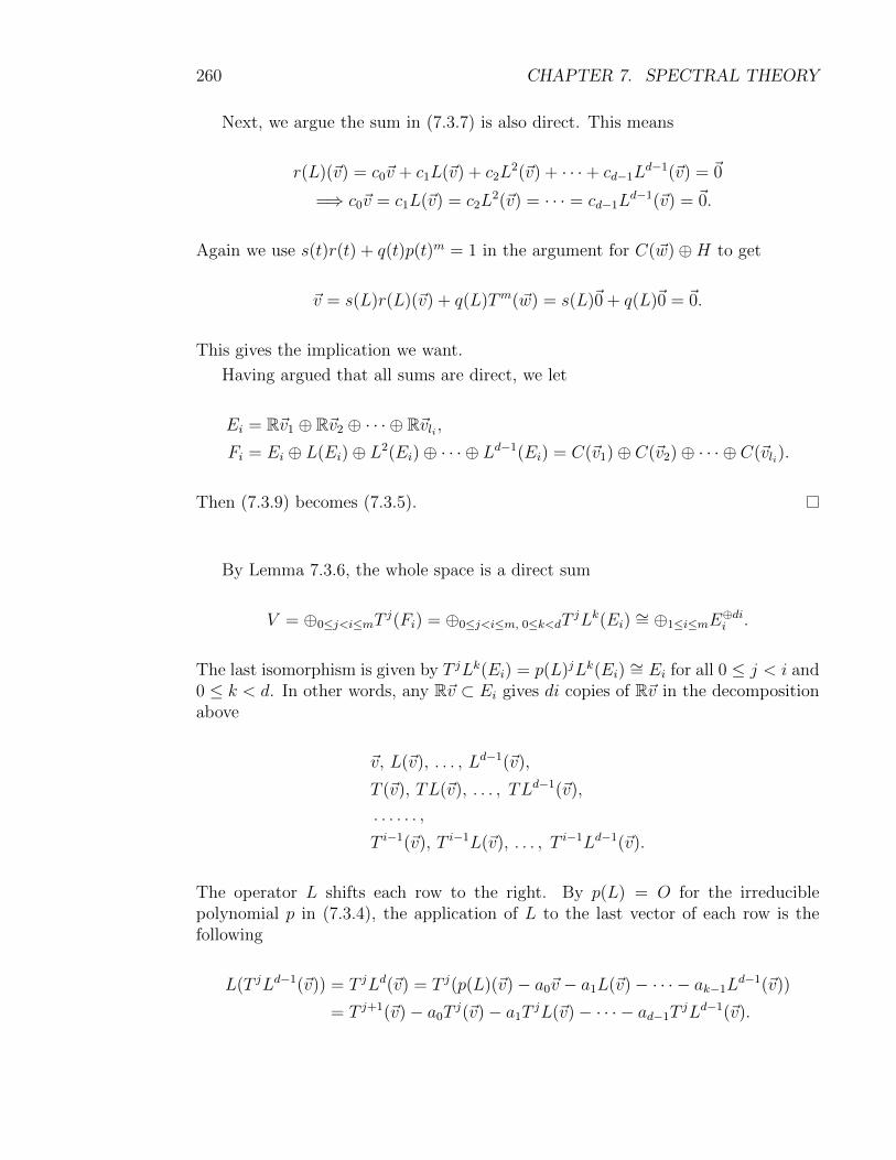
260 CHAPTER 7. SPECTRAL THEORY
Next, we argue the sum in (7.3.7) is also direct. This means
r(L)(~v) = c0~v + c1L(~v) + c2L2(~v) + · · ·+ cd−1L
d−1(~v) = ~0
=⇒ c0~v = c1L(~v) = c2L2(~v) = · · · = cd−1L
d−1(~v) = ~0.
Again we use s(t)r(t) + q(t)p(t)m = 1 in the argument for C(~w)⊕H to get
~v = s(L)r(L)(~v) + q(L)Tm(~w) = s(L)~0 + q(L)~0 = ~0.
This gives the implication we want.
Having argued that all sums are direct, we let
Ei = R~v1 ⊕ R~v2 ⊕ · · · ⊕ R~vli ,Fi = Ei ⊕ L(Ei)⊕ L2(Ei)⊕ · · · ⊕ Ld−1(Ei) = C(~v1)⊕ C(~v2)⊕ · · · ⊕ C(~vli).
Then (7.3.9) becomes (7.3.5).
By Lemma 7.3.6, the whole space is a direct sum
V = ⊕0≤j<i≤mTj(Fi) = ⊕0≤j<i≤m, 0≤k<dT
jLk(Ei) ∼= ⊕1≤i≤mE⊕dii .
The last isomorphism is given by T jLk(Ei) = p(L)jLk(Ei) ∼= Ei for all 0 ≤ j < i and0 ≤ k < d. In other words, any R~v ⊂ Ei gives di copies of R~v in the decompositionabove
~v, L(~v), . . . , Ld−1(~v),
T (~v), TL(~v), . . . , TLd−1(~v),
. . . . . . ,
T i−1(~v), T i−1L(~v), . . . , T i−1Ld−1(~v).
The operator L shifts each row to the right. By p(L) = O for the irreduciblepolynomial p in (7.3.4), the application of L to the last vector of each row is thefollowing
L(T jLd−1(~v)) = T jLd(~v) = T j(p(L)(~v)− a0~v − a1L(~v)− · · · − ak−1Ld−1(~v))
= T j+1(~v)− a0Tj(~v)− a1T
jL(~v)− · · · − ad−1TjLd−1(~v).
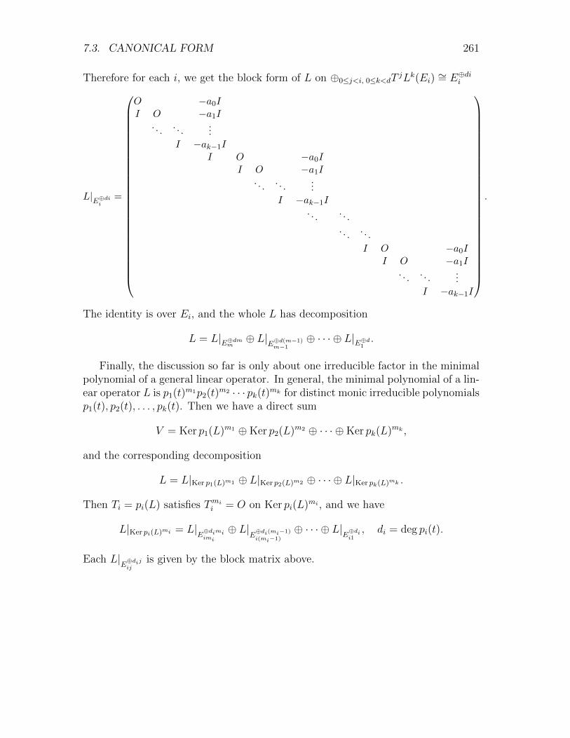
7.3. CANONICAL FORM 261
Therefore for each i, we get the block form of L on ⊕0≤j<i, 0≤k<dTjLk(Ei) ∼= E⊕dii
L|E⊕dii=
O −a0II O −a1I
. . .. . .
...I −ak−1I
I O −a0II O −a1I
. . .. . .
...I −ak−1I
. . .. . .. . .
. . .
I O −a0II O −a1I
. . .. . .
...I −ak−1I
.
The identity is over Ei, and the whole L has decomposition
L = L|E⊕dmm⊕ L|
E⊕d(m−1)m−1
⊕ · · · ⊕ L|E⊕d1.
Finally, the discussion so far is only about one irreducible factor in the minimalpolynomial of a general linear operator. In general, the minimal polynomial of a lin-ear operator L is p1(t)m1p2(t)m2 · · · pk(t)mk for distinct monic irreducible polynomialsp1(t), p2(t), . . . , pk(t). Then we have a direct sum
V = Ker p1(L)m1 ⊕Ker p2(L)m2 ⊕ · · · ⊕Ker pk(L)mk ,
and the corresponding decomposition
L = L|Ker p1(L)m1 ⊕ L|Ker p2(L)m2 ⊕ · · · ⊕ L|Ker pk(L)mk .
Then Ti = pi(L) satisfies Tmii = O on Ker pi(L)mi , and we have
L|Ker pi(L)mi = L|E⊕dimiimi
⊕ L|E⊕di(mi−1)
i(mi−1)
⊕ · · · ⊕ L|E⊕dii1, di = deg pi(t).
Each L|E⊕dijij
is given by the block matrix above.

262 CHAPTER 7. SPECTRAL THEORY

Chapter 8
Tensor
8.1 Bilinear
8.1.1 Bilinear Map
Let U, V,W be vector spaces. A map B : V ×W → U is bilinear if it is linear in Uand linear in V
B(x1~v1 + x2~v2, ~w) = x1B(~v1, ~w) + x2B(~v2, ~w),
B(~v, y1 ~w1 + y2 ~w2) = y1B(~v, ~w1) + y2B(~v, ~w2).
In case U = F, the bilinear map is a bilinear function b(~x, ~y).The bilinear property extends to
B(x1~v1 + x2~v2 + · · ·+ xm~vm, y1 ~w1 + y2 ~w2 + · · ·+ yn ~wn) =∑
1≤i≤m1≤j≤n
xiyjB(~vi, ~wj).
If α = {~v1, ~v2, . . . , ~vm} and β = {~w1, ~w2, . . . , ~wn} are bases of V and W , then theformula above shows that bilinear maps B are in one-to-one correspondence withthe collection of values B(~vi, ~wj) on bases. These values form an m× n “matrix”
[B]αβ = (Bij), Bij = B(~vi, ~wj).
In case U = F, we denote bij = b(~vi, ~wj), and get
b(~x, ~y) =∑i,j
bijxiyj = [~x]Tα [b]αβ[~y]β.
We may define linear combination of bilinear maps V ×W → U is obvious way.This makes all the bilinear maps into a vector space Bilinear(V ×W,U). On theother hand, we may regard a bilinear map as a linear transformation
~v 7→ B(~v, ·) : V → Hom(W,U).
263

264 CHAPTER 8. TENSOR
We may also regard a bilinear map as another linear transformation
~w 7→ B(·, ~w) : W → Hom(V, U).
The three viewpoints are equivalent. This means we have an isomorphism of vectorspaces
Hom(V,Hom(W,U)) ∼= Bilinear(V ×W,U) ∼= Hom(W,Hom(V, U)).
Example 8.1.1. In a real inner product space, the inner product is a bilinear func-tion 〈·, ·〉 : V × V → R. The complex inner product is not bilinear because it isconjugate linear in the second vector. The matrix of the inner product with respectto an orthonormal basis α is [〈·, ·〉]αα = I.
Example 8.1.2. Recall the dual space V ∗ = Hom(V,F) of linear functionals on anF-vector space V . The evaluation pairing
b(~x, l) = l(~x) : V × V ∗ → F
is a bilinear function. The corresponding map for the second vector V ∗ → Hom(V,F)is the identity. The corresponding map for the first vector V → Hom(V ∗,F) = V ∗∗
is ~v 7→ ~v∗∗, ~v∗∗(l) = l(~v).
Example 8.1.3. The cross product in R3
(x1, x2, x3)× (y1, y2, y3) = (x2y3 − x3y2, x3y1 − x1y3, x1y2 − x2y1)
is a bilinear map, with ~ei × ~ej) = ±~ek when i, j, k are distinct, and ~ei × ~ei = ~0. Thesign ± is given by the orientation of the basis {~ei, ~ej, ~ek}. The cross product alsohas the alternating property ~x× ~y = −~y × ~x.
Example 8.1.4. Composiiton of linear transform. Product of matrix.
Exercise 8.1. For matching linear transformations L, show that the compositionsB(L(~v), ~w),B(~v, L(~w)), L(B(~v, ~w)) are still linear transformations.
Exercise 8.2. Show that a bilinear map B : V ×W → U1⊕U2 is given by two bilinear mapsB1 : V ×W → U1 and B2 : V ×W → U2. What if V or W is a direct sum?
Exercise 8.3. Show that a map B : V ×W → Fn is bilinear if and only if each coordinatebi : V ×W → F of B is a bilinear function.
Exercise 8.4. For a linear functional l(x1, x2, x3) = a1x1 +a2x2 +a3x3, what is the bilinearfunction l(~x× ~y)?

8.1. BILINEAR 265
8.1.2 Bilinear Function
A bilinear function b : V × W → F is determined by its values bij = b(~vi, ~wj) onbases α = {~v1, . . . , ~vm} and β = {~w1, . . . , ~wn} of V and W
b(~x, ~y) =∑i,j
bijxiyj = [~x]TαB[~y]β, [~x]α = (x1, . . . , xm), [~y]β = (y1, . . . , yn).
Here the matrix of bilinear function is
B = [b]αβ = (b(~vi, ~wj))m,ni,j=1.
By b(~x, ~y) = [~x]Tα [b]αβ[~y]β and [~x]α′ = [I]α′α[~x]α, we get the change of matrix causedby the change of bases
[b]α′β′ = [I]Tαα′ [b]αβ[I]ββ′ .
A bilinear function induces a linear transformation
L(~v) = b(~v, ·) : V → W ∗.
Conversely, a linear transformation L : V → W ∗ gives a bilinear function b(~v, ~w) =L(~v)(~w).
If W is a real inner product space, then we have the induced isomorphism W ∗ ∼=W by Proposition 4.3.1. Combined with the linear transformation above, we get alinear transformation, still denoted L
L : V → W ∗ ∼= W, ~v 7→ b(~v, ·) = 〈L(~v), ·〉.
This meansb(~v, ~w) = 〈L(~v), ~w〉 for all ~v ∈ V, ~w ∈ W.
Therefore real bilinear functions b : V ×W → R are in one-to-one correspondencewith linear transformations L : V → W .
Similarly, the bilinear function also corresponds to a linear transformation
L∗(~w) = b(·, ~w) : W → V ∗.
The reason for the notation L∗ is that the linear transformation is W ∼= W ∗∗ L∗−→ V ∗,or the dual linear transformation up to the natural double dual isomorphism of W .If we additionally know that V is a real inner product space, then we may combineW → V ∗ with the isomorphism V ∗ ∼= V by Proposition 4.3.1, to get the followinglinear transformation, still denoted L∗
L∗ : W → V ∗ ∼= V, ~w 7→ b(·, ~w) = 〈·, L∗(~w)〉.
This meansb(~v, ~w) = 〈~v, L∗(~w)〉 for all ~v ∈ V, ~w ∈ W.
If both V and W are real inner product spaces, then we have
b(~v, ~w) = 〈L(~v), ~w〉 = 〈~v, L∗(~w)〉.

266 CHAPTER 8. TENSOR
Exercise 8.5. What are the matrices of bilinear functions b(L(~v), ~w), b(~v, L(~w)), l(B(~v, ~w))?
Example 8.1.5. An inner product 〈·, ·〉 : V ×V → R is a dual pairing. The inducedisomorphism
V ∼= V ∗ : ~a 7→ 〈~a, ·〉
makes V into a self dual vector space. In a self dual vector space, it makes sense toask for self dual basis. For inner product, a basis α is self dual if
〈~vi, ~vj〉 = δij.
This means exactly that the basis is orthonormal.
Example 8.1.6. The evaluation pairing in Example 8.1.2 is a dual pairing. For abasis α of V , the dual basis with respect to the evaluation pairing is the dual basisα∗ in Section 2.4.1.
Example 8.1.7. The function space is infinite dimensional. Its dual space needs toconsider the topology, which means that the dual space consists of only continuouslinear functionals. For the vector space of power p integrable functions
Lp[a, b] = {f(t) :
∫ b
a
|f(t)|pdt <∞}, p ≥ 1,
the continuous linear functionals on Lp[a, b] are of the form
l(f) =
∫ b
a
f(t)g(t)dt,
where the function g(t) satisfies∫ b
a
|g(t)|qdt <∞, 1
p+
1
q= 1.
This shows that the dual space Lp[a, b]∗ of all continuous linear functionals on Lp[a, b]is Lq[a, b]. In particular, the Hilbert space L2[a, b] of square integrable functions isself dual.
8.1.3 Quadratic Form
A quadratic form on a vector space V is q(~x) = b(~x, ~x), where b is some bilinearfunction on V ×V . Since replacing b with the symmetric bilinear function 1
2(b(~x, ~y)+
b(~y, ~x)) gives the same q, we will always take b to be symmetric
b(~x, ~y) = b(~y, ~x).

8.1. BILINEAR 267
Then (the symmetric) b can be recovered from q by polarisation
b(~x, ~y) =1
4(q(~x+ ~y)− q(~x− ~y)) =
1
2(q(~x+ ~y)− q(~x)− q(~y)).
The discussion assumes that 2 is invertible in the base field F. If this is not thecase, then there is a subtle difference between quadratic forms and symmetric forms.The subsequent discussion always assumes that 2 is invertible.
The matrix of q with respect to a basis α = {~v1, . . . , ~vn} is the matrix of b withrespect to the basis, and is symmetric
[q]α = [b]αα = B = (b(~vi, ~vj)).
Then the quadratic form can be expressed in terms of the α-coordinate [~x]α =(x1, . . . , xn)
q(~x) = [~x]Tα [q]α[~x]α =∑
1≤i≤n
biix2i + 2
∑1≤i<j≤n
bijxixj.
For another basis β, we have
[q]β = [I]Tαβ[q]α[I]αβ = P TBP, P = [I]αβ.
In particular, the rank of a quadratic form is well defined
rank q = rank[q]α.
Exercise 8.6. Prove that a function is a quadratic form if and only if it is homogeneous ofsecond order
q(c~x) = c2q(~x),
and satisfies the parallelogram identity
q(~x+ ~y) + q(~x− ~y) = 2q(~x) + 2q(~y).
Similar to the diagonalisation of linear operators, we may ask about the canonicalforms of quadratic forms. The goal is to eliminate the cross terms bijxixj, i 6= j,by choosing a different basis. Then the quadratic form consists of only the squareterms
q(~x) = b1x21 + · · ·+ bnx
2n.
We may get the canonical form by the method of completing the square. Themethod is a version of Gaussian elimination, and can be applied to any base field Fin which 2 is invertible.
In terms of matrix, this means that we want to express a symmetric matrix Bas P TDP for diagonal D and invertible P .
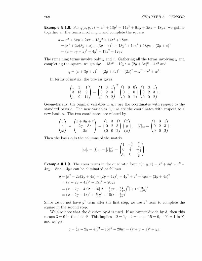
268 CHAPTER 8. TENSOR
Example 8.1.8. For q(x, y, z) = x2 + 13y2 + 14z2 + 6xy + 2xz + 18yz, we gathertogether all the terms involving x and complete the square
q = x2 + 6xy + 2xz + 13y2 + 14z2 + 18yz
= [x2 + 2x(3y + z) + (3y + z)2] + 13y2 + 14z2 + 18yz − (3y + z)2
= (x+ 3y + z)2 + 4y2 + 13z2 + 12yz.
The remaining terms involve only y and z. Gathering all the terms involving y andcompleting the square, we get 4y2 + 13z2 + 12yz = (2y + 3z)2 + 4z2 and
q = (x+ 3y + z)2 + (2y + 3z)2 + (2z)2 = u2 + v2 + w2.
In terms of matrix, the process gives1 3 13 13 91 9 14
=
1 3 10 2 30 0 2
T 1 0 00 1 00 0 1
1 3 10 2 30 0 2
.
Geometrically, the original variables x, y, z are the coordinates with respect to thestandard basis ε. The new variables u, v, w are the coordinates with respect to anew basis α. The two coordinates are related byuv
w
=
x+ 3y + z2y + 3z
2z
=
1 3 10 2 30 0 2
xyz
, [I]αε =
1 3 10 2 30 0 2
.
Then the basis α is the columns of the matrix
[α]ε = [I]εα = [I]−1αε =
1 −32
74
0 12−3
4
0 0 12
.
Example 8.1.9. The cross terms in the quadratic form q(x, y, z) = x2 + 4y2 + z2 −4xy − 8xz − 4yz can be eliminated as follows
q = [x2 − 2x(2y + 4z) + (2y + 4z)2] + 4y2 + z2 − 4yz − (2y + 4z)2
= (x− 2y − 4z)2 − 15z2 − 20yz
= (x− 2y − 4z)2 − 15[z2 + 43yz +
(23y)2
] + 15(
23y)2
= (x− 2y − 4z)2 + 203y2 − 15(z + 2
3y)2.
Since we do not have y2 term after the first step, we use z2 term to complete thesquare in the second step.
We also note that the division by 3 is used. If we cannot divide by 3, then thismeans 3 = 0 in the field F. This implies −2 = 1, −4 = −4, −15 = 0, −20 = 1 in F,and we get
q = (x− 2y − 4z)2 − 15z2 − 20yz = (x+ y − z)2 + yz.

8.1. BILINEAR 269
We may further eliminate the cross terms by introducing y = u + v, z = u − v, sothat
q = (x+ y − z)2 + u2 − v2 = (x+ y − z)2 + 14(y + z)2 − 1
4(y − z)2.
Example 8.1.10. The quadratic form q = xy + yz has no square term. We mayeliminate the cross terms by introducing x = u+ v, y = u− v, so that q = u2− v2 +uz − vz. Then we complete the square and get
q =(u− 1
2z)2 −
(v + 1
2z)2
= 14(x+ y − z)2 − 1
4(x− y + z)2.
Example 8.1.11. The cross terms in the quadratic form
q = 4x21 + 19x2
2 − 4x24
− 4x1x2 + 4x1x3 − 8x1x4 + 10x2x3 + 16x2x4 + 12x3x4
can be eliminated as follows
q = 4[x21 − x1x2 + x1x3 − 2x1x4] + 19x2
2 − 4x24 + 10x2x3 + 16x2x4 + 12x3x4
= 4[x2
1 + 2x1
(−1
2x2 + 1
2x3 − x4
)+(−1
2x2 + 1
2x3 − x4
)2]
+ 19x22 − 4x2
4 + 10x2x3 + 16x2x4 + 12x3x4 − 4(−1
2x2 + 1
2x3 − x4
)2
= 4(x1 − 1
2x2 + 1
2x3 − x4
)2+ 18
[x2
2 + 23x2x3 + 2
3x2x4
]− x2
3 − 8x24 + 16x3x4
= (2x1 − x2 + x3 − 2x4)2 + 18[x2
2 + 2x2
(13x3 + 1
3x4
)+(
13x3 + 1
3x4
)2]
− x23 − 8x2
4 + 16x3x4 − 18(
13x3 + 1
3x4
)2
= (2x1 − x2 + x3 − 2x4)2 + 18(x2 + 1
3x3 + 1
3x4
)2 − 3(x23 − 4x3x4)− 10x2
4
= (2x1 − x2 + x3 − 2x4)2 + 2(3x2 + x3 + x4)2
− 3[x23 + 2x3(−2x4) + (−2x4)2]− 10x2
4 + 3(−2x4)2
= (2x1 − x2 + x3 − 2x4)2 + 2(3x2 + x3 + x4)2 − 3(x3 − 2x4)2 + 2x24
= y21 + 2y2
2 − 3y33 + 2y2
4.
The new variables y1, y2, y3, y4 are the coordinates with respect to the basis of thecolumns of
2 −1 1 −20 3 1 10 0 1 −20 0 0 1
−1
=
12
16−2
3−1
2
0 13−1
3−1
0 0 1 20 0 0 1
.
Example 8.1.12. For the quadratic form q(x, y, z) = x2 +iy2 +3z2 +2(1+i)xy+4yz

270 CHAPTER 8. TENSOR
over complex numbers C, the following eliminates the cross terms
q = [x2 + 2(1 + i)xy + ((i+ 1)y)2] + iy2 + 3z2 + 4yz − (i+ 1)2y2
= (x+ (1 + i)y)2 − iy2 + 3z2 + 4yz
= (x+ (1 + i)y)2 − i[y2 + 4iyz + (2iz)2
]+ 3z2 + i(2i)2z2
= (x+ (1 + i)y)2 − i(y + 2iz)2 + (3− 4i)z2.
We may further use (pick one of two possible complex square roots)
√−i =
√e−i
π2 = e−i
π4 = 1−i√
2,√
3− 4i =√
(2− i)2 = 2− i,
to get
q = (x+ (1 + i)y)2 +(
1−i√2y +√
2(1 + i)z)2
+ ((2− i)z)2.
In terms of matrix, the process gives 1 1 + i 01 + i i 2
0 2 3
=
1 1 + i 0
0 1−i√2
√2(1 + i)
0 0 2− i
T 1 0 00 1 00 0 1
1 1 + i 0
0 1−i√2
√2(1 + i)
0 0 2− i
.
The new variables x+ (1 + i)y, 1−i√2y +√
2(1 + i)z, (2− i)z are the coordinates withrespect to some new basis. By the row operation1 1 + i 0 1 0 0
0 1−i√2
√2(1 + i) 0 1 0
0 0 2− i 0 0 1
1+i√2R2
−−−→2+i5R3
1 1 + i 0 1 0 00 1 2i 0 1+i√
20
0 0 1 0 0 2+i5
R2−2iR3−−−−−→
1 1 + i 0 1 0 00 1 0 0 1+i√
2−2+4i
5
0 0 1 0 0 2+i5
R1−(1+i)R2−−−−−−−→
1 0 0 1√
2i −6+2i5
0 1 0 0 1+i√2
−2+4i5
0 0 1 0 0 2+i5
,
the new basis is the last three columns of last matrix above.
Exercise 8.7. Eliminate the cross terms.
1. x2 + 4xy − 5y2.
2. 2x2 + 4xy.
3. 4x21 + 4x1x2 + 5x2
2.
4. x2 + 2y2 + z2 + 2xy − 2xz.
5. −2u2 − v2 − 6w2 − 4uw + 2vw.
6. x21 + x2
3 + 2x1x2 + 2x1x3 + 2x1x4 + 2x3x4.
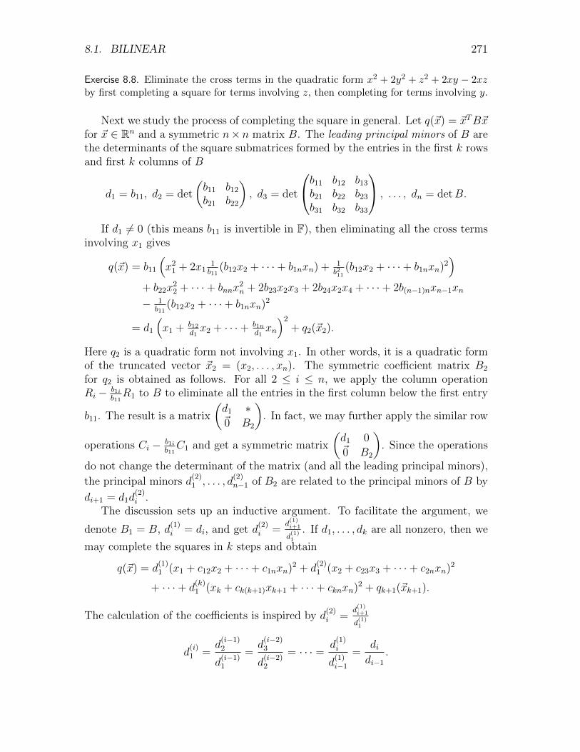
8.1. BILINEAR 271
Exercise 8.8. Eliminate the cross terms in the quadratic form x2 + 2y2 + z2 + 2xy − 2xzby first completing a square for terms involving z, then completing for terms involving y.
Next we study the process of completing the square in general. Let q(~x) = ~xTB~xfor ~x ∈ Rn and a symmetric n× n matrix B. The leading principal minors of B arethe determinants of the square submatrices formed by the entries in the first k rowsand first k columns of B
d1 = b11, d2 = det
(b11 b12
b21 b22
), d3 = det
b11 b12 b13
b21 b22 b23
b31 b32 b33
, . . . , dn = detB.
If d1 6= 0 (this means b11 is invertible in F), then eliminating all the cross termsinvolving x1 gives
q(~x) = b11
(x2
1 + 2x11b11
(b12x2 + · · ·+ b1nxn) + 1b211
(b12x2 + · · ·+ b1nxn)2)
+ b22x22 + · · ·+ bnnx
2n + 2b23x2x3 + 2b24x2x4 + · · ·+ 2b(n−1)nxn−1xn
− 1b11
(b12x2 + · · ·+ b1nxn)2
= d1
(x1 + b12
d1x2 + · · ·+ b1n
d1xn
)2
+ q2(~x2).
Here q2 is a quadratic form not involving x1. In other words, it is a quadratic formof the truncated vector ~x2 = (x2, . . . , xn). The symmetric coefficient matrix B2
for q2 is obtained as follows. For all 2 ≤ i ≤ n, we apply the column operationRi − b1i
b11R1 to B to eliminate all the entries in the first column below the first entry
b11. The result is a matrix
(d1 ∗~0 B2
). In fact, we may further apply the similar row
operations Ci − b1ib11C1 and get a symmetric matrix
(d1 0~0 B2
). Since the operations
do not change the determinant of the matrix (and all the leading principal minors),
the principal minors d(2)1 , . . . , d
(2)n−1 of B2 are related to the principal minors of B by
di+1 = d1d(2)i .
The discussion sets up an inductive argument. To facilitate the argument, we
denote B1 = B, d(1)i = di, and get d
(2)i =
d(1)i+1
d(1)1
. If d1, . . . , dk are all nonzero, then we
may complete the squares in k steps and obtain
q(~x) = d(1)1 (x1 + c12x2 + · · ·+ c1nxn)2 + d
(2)1 (x2 + c23x3 + · · ·+ c2nxn)2
+ · · ·+ d(k)1 (xk + ck(k+1)xk+1 + · · ·+ cknxn)2 + qk+1(~xk+1).
The calculation of the coefficients is inspired by d(2)i =
d(1)i+1
d(1)1
d(i)1 =
d(i−1)2
d(i−1)1
=d
(i−2)3
d(i−2)2
= · · · = d(1)i
d(1)i−1
=didi−1
.
272 CHAPTER 8. TENSOR
Moreover, the coefficient of x2k+1 in qk+1 is d
(k+1)1 =
dk+1
dk.
Proposition 8.1.1 (Lagrange-Beltrami Identity). Suppose q(~x) = ~xTB~x is a quadraticform of rank r, over a field in which 2 6= 0. If all the leading principal minorsd1, . . . , dr of the symmetric coefficient matrix B are nonzero, then there is an uppertriangular change of variables
yi = xi + ci(i+1)xi+1 + · · ·+ cinxn, i = 1, . . . , r,
such that
q = d1y21 +
d2
d1
y22 + · · ·+ dr
dr−1
y2r .
Examples 8.1.9 and 8.1.10 shows that the nonzero condition on leading principalminors may not always be satisfied. Still, the examples show that it is alwayspossible to eliminate cross terms after a suitable change of variable.
Proposition 8.1.2. Any quadratic form of rank r and over a field in which 2 6= 0can be expressed as
q = b1x21 + · · ·+ brx
2r
after a suitable change of variable.
In terms of matrix, this means that any symmetric matrix B can be written asB = P TDP , where P is invertible and B is a diagonal matrix with exactly r nonzeroentries. For F = C, we may further get the unique canonical form by replacing xiwith
√bixi
q = x21 + · · ·+ x2
r, r = rank q.
Two quadratic forms q and q′ are equivalent if q′(~x) = q(L(~x)) for some invertiblelinear transformation. In terms of symmetric matrices, this means that S and P TSPare equivalent. The unique canonical form above implies the following.
Theorem 8.1.3. Two complex quadratic forms are equivalent if and only if theyhave the same rank.
For F = R, we may replace xi with√bixi in case bi > 0 and with
√−bixi in case
bi < 0. The canonical form we get is (after rearranging the order of xi if needed)
q = x21 + · · ·+ x2
s − x2s+1 − · · · − x2
r.
Theorem 8.2.4 discusses this canonical form.

8.2. HERMITIAN 273
8.2 Hermitian
8.2.1 Sesquilinear Function
The complex inner product is not bilinear. It is a sesquilinear function (defined forcomplex vector spaces V and W ) in the following sense
s(x1~v1 + x2~v2, ~w) = x1s(~v1, ~w) + x2s(~v2, ~w),
s(~v, y1 ~w1 + y2 ~w2) = y1s(~v, ~w1) + y2s(~v, ~w2).
The sesquilinear function can be regarded as a bilinear function s : V × W → C,where W is the conjugate vector space of W .
A sesquilinear function is determined by its values sij = s(~vi, ~wj) on bases α ={~v1, . . . , ~vm} and β = {~w1, . . . , ~wn} of V and W
s(~x, ~y) =∑i,j
sijxiyj = [~x]TαS[~y]β, [~x]α = (x1, . . . , xm), [~y]β = (y1, . . . , yn).
Here the matrix of sesquilinear function is
S = [s]αβ = (s(~vi, ~wj))m,ni,j=1.
By s(~x, ~y) = [~x]Tα [s]αβ[~y]β and [~x]α′ = [I]α′α[~x]α, we get the change of matrix causedby the change of bases
[s]α′β′ = [I]Tαα′ [s]αβ[I]ββ′ .
A sesquilinear function s : V ×W → C induces a linear transformation
L(~v) = s(~v, ·) : V → W ∗ = Hom(W,C) = Hom(W ,C).
Here W ∗ is the conjugate dual space consisting of conjugate linear functionals. Wehave a one-to-one correspondence between sesquilinear functions s and linear trans-formations L.
If we also know that W is a complex (Hermitian) inner product space, thenwe have a linear isomorphism ~w 7→ 〈~w, ·〉 : W ∼= W ∗, similar to Proposition 4.3.1.Combined with the linear transformation above, we get a linear transformation, stilldenoted L
L : V → W ∗ ∼= W, ~v 7→ s(~v, ·) = 〈L(~v), ·〉.
This meanss(~v, ~w) = 〈L(~v), ~w〉 for all ~v ∈ V, ~w ∈ W.
Therefore sesquilinear functions s : V ×W → C are in one-to-one correspondencewith linear transformations L : V → W .
The sesquilinear function also induces a conjugate linear transformation
L∗(~w) = s(·, ~w) : W → V ∗ = Hom(V,C),

274 CHAPTER 8. TENSOR
The correspondence s 7→ L∗ is again one-to-one if V and W have finite dimensions.If we also know V is a complex inner product space, then we have a conjugate linearisomorphism ~v 7→ 〈·, ~v〉 : V ∼= V ∗, similar to Proposition 4.3.1. Combined with theconjugate linear transformation above, we get a linear transformation, still denotedL∗
L∗ : W → V ∗ ∼= V, ~w 7→ s(·, ~w) = 〈·, L(~w)〉.This means
s(~v, ~w) = 〈~v, L∗(~w)〉 for all ~v ∈ V, ~w ∈ W.Therefore sesquilinear functions s : V ×W → C are in one-to-one correspondencewith linear transformations L∗ : W → V .
If both V and W are complex inner product spaces, then we have
s(~v, ~w) = 〈L(~v), ~w〉 = 〈~v, L∗(~w)〉.
Exercise 8.9. Suppose s(~x, ~y) is sesquilinear. Prove that s(~y, ~x) is also sesquilinear. Whatare the linear transformations induced by s(~y, ~x)? How are the matrices of the twosesquilinear functions related?
A sesquilinear function is a conjugate dual pairing if both L : V → W ∗ andL∗ : W → V ∗ are isomorphisms. In fact, one isomorphism implies the other. This isalso the same as both are one-to-one, or both are onto.
The basic examples of conjugate dual pairing are the complex inner product andthe evaluation pairing
s(~x, l) = l(~x) : V × V ∗ → C.A basis α = {~v1, . . . , ~vn} of V and a basis β = {~w1, . . . , ~wn} of W are dual baseswith respect to the dual pairing if
s(~vi, ~wj) = δij, or [s]αβ = I.
We may express any ~x ∈ V in terms of α
~x = s(~x, ~w1)~v1 + s(~x, ~w2)~v2 + · · ·+ s(~x, ~wn)~vn,
and express any ~y ∈ W in terms of β
~y = s(~v1, ~y)~w1 + s(~v2, ~y)~w2 + · · ·+ s(~vn, ~y)~wn,
For the inner product, a basis is self dual if and only if it is an orthonormalbasis. For the evaluation pairing, the dual basis α∗ = {~v∗1, . . . , ~v∗n} ⊂ V ∗ of α ={~v1, . . . , ~vn} ⊂ V is given by
~v∗i (~x) = xi, [~x]α = (x1, . . . , xn).
Exercise 8.10. Suppose a sesquilinear form s : V ×W → C is a dual pairing. Suppose αand β are bases of V and W . Prove that the following are equivalent.

8.2. HERMITIAN 275
1. α and β are dual bases with respect to s.
2. L takes α to β∗ (conjugate dual basis of W ∗).
3. L∗ takes β to α∗ (dual basis of V ∗).
Exercise 8.11. Prove that if α and β are dual bases with respect to dual pairing s(~x, ~y),then β and α are dual bases with respect to s(~y, ~x).
Exercise 8.12. Suppose α and β are dual bases with respect to a sesquilinear dual pairings : V ×W → C. What is the relation between matrices [s]αβ, [L]β∗α, [L∗]α∗β?
8.2.2 Hermitian Form
A sesquilinear function s : V × V → C is Hermitian if it satisfies
s(~x, ~y) = s(~y, ~x).
A typical example is the complex inner product. If we take ~x = ~y, then we get aHermitian form
q(~x) = s(~x, ~x).
Conversely, the Hermitian sesquilinear function s can be recovered from q by polar-isation (see Exercise 6.21)
s(~x, ~y) = 14(q(~x+ ~y)− q(~x− ~y) + iq(~x+ i~y)− iq(~x− i~y)).
Proposition 8.2.1. A sesquilinear function s(~x, ~y) is Hermitian if and only if s(~x, ~x)is always a real number.
Exercise 6.25 is a similar result.
Proof. If s is Hermitian, then s(~x, ~y) = s(~y, ~x) implies s(~x, ~x) = s(~x, ~x), which meanss(~x, ~x) is a real number.
Conversely, suppose s(~x, ~x) is always a real number. We want to show s(~x, ~y) =s(~y, ~x), which is the same as s(~x, ~y)+s(~y, ~x) is real and s(~x, ~y)−s(~y, ~x) is imaginary.This follows from
s(~x, ~y) + s(~y, ~x) = s(~x+ ~y, ~x+ ~y)− s(~x, ~x)− s(~y, ~y)
is(~x, ~y)− is(~y, ~x) = s(i~x+ ~y, i~x+ ~y)− s(i~x, i~x)− s(~y, ~y).
In terms of the matrix S = [q]α = [s]αα with respect to a basis α of V , theHermitian property means that S∗ = S, or S is a Hermitian matrix. For anotherbasis β, we have
[q]β = [I]Tαβ[q]α[I]αβ = P ∗SP, P = [I]αβ.

276 CHAPTER 8. TENSOR
Suppose V is an inner product space. Then the Hermitian form is given by alinear operator L by q(~x) = 〈L(~x), ~x〉. By Proposition 8.2.1, we know q(~x) is a realnumber, and therefore q(~x) = 〈L(~x), ~x〉 = 〈~x, L(~x)〉. By polarisation, we get
〈L(~x), ~y〉 = 〈~x, L(~y)〉 for all ~x, ~y.
This means that Hermitian forms are in one-to-one correspondence with self-adjointoperators.
By Propositions 7.2.6 and 7.2.7, L has an orthonormal basis α = {~v1, . . . , ~vn}of eigenvectors, with eigenvalues d1, . . . , dn. Then we have 〈L(~vi), ~vj〉 = 〈di~vi, ~vj〉 =diδij. This means
[q]α =
d1
. . .
dn
is diagonal, and the expression of q in α-coordinate has no cross terms
q(~x) = d1x1x1 + · · ·+ dnxnxn = d1|x1|2 + · · ·+ dn|xn|2.
Let λmax = max di and λmin = min di be the maximal and minimal eigenvaluesof L. Then the formula above implies (‖~x‖2 = |x1|2 + · · · + |xn|2 by orthonormalbasis)
λmin‖~x‖2 ≤ q(~x) = 〈L(~x), ~x〉 ≤ λmax‖~x‖2.
Moreover, the right equality is reached if and only if xi = 0 whenever di 6= λmax.Since⊕di=λR~vi = Ker(L−λI), the right equality is reached exactly on the eigenspaceKer(L − λmaxI). Similarly, the left equality is reached exactly on the eigenspaceKer(L− λminI).
Proposition 8.2.2. For self-adjoint operator L on an inner product space, the max-imal and minimal eigenvalues of L are max‖~x‖=1〈L(~x), ~x〉 and min‖~x‖=1〈L(~x), ~x〉.
Proof. We provide an alternative proof by using the Lagrange multiplier. We tryto find the maximum of the function q(~x) = 〈L(~x), ~x〉 = 〈~x, L(~x)〉 subject to theconstraint g(~x) = 〈~x, ~x〉 = ‖~x‖2 = 1. By
q(~x0 + ∆~x) = 〈L(~x0 + ∆~x), ~x0 + ∆~x〉= 〈L(~x0), ~x0〉+ 〈L(~x0),∆~x〉+ 〈L(∆~x), ~x0〉+ 〈L(∆~x),∆~x〉= q(~x0) + 〈L(~x0),∆~x〉+ 〈∆~x, L(~x0)〉+ o(‖∆~x‖),
we get (the “multi-derivative” is a linear functional)
q′(~x0) = 〈L(~x0), ·〉+ 〈·, L(~x0)〉.
By the similar reason, we have
g′(~x0) = 〈~x0, ·〉+ 〈·, ~x0〉.

8.2. HERMITIAN 277
If the maximum of q subject to the constraint g = 1 happens at ~x0, then we have
q′(~x0) = 〈L(~x0), ·〉+ 〈·, L(~x0)〉 = 〈λ~x0, ·〉+ 〈·, λ~x0〉 = λg′(~x0)
for a real number λ. Let ~v = L(~x0)−λ~x0. Then the equality means 〈~v, ·〉+〈·, ~v〉 = 0.Taking the variable · to be ~v, we get 2‖~v‖2 = 0, or ~v = ~0. This proves thatL(~x0) = λ~x0. Moreover, the maximum is
max‖~x‖=1
q(~x) = q(~x0) = 〈L(~x0), ~x0〉 = 〈λ~x0, ~x0〉 = λg(~x0) = λ.
For any other eigenvalue µ, we have L(~x) = µ~x for a unit length vector ~x and get
µ = µ〈~x, ~x〉 = 〈µ~x, ~x〉 = 〈L(~x), ~x〉 = q(~x) ≤ q(~x0) = λ.
This proves that λ is the maximum eigenvalue.
Example 8.2.1. In Example 7.2.1, we have the orthogonal diagonalisation of a Her-mitian matrix(
2 1 + i1− i 3
)=
(1+i√
31√3
− 1√3
1−i√3
)(1 00 4
)( 1+i√3
1√3
− 1√3
1−i√3
)−1
=
(1−i√
3− 1√
31√3
1+i√3
)∗(1 00 4
)(1−i√3− 1√
31√3
1+i√3
).
In terms of Hermitian form, this means
2xx+ (1 + i)xy + (1− i)yx+ 3yy =∣∣∣ 1√
3((1− i)x− y)
∣∣∣2 + 4∣∣∣ 1√
3(x+ (1 + i)y)
∣∣∣2 .Example 8.2.2. In Example 7.2.4, we found an orthogonal diagonalisation of thesymmetric matrix in Example 7.1.14
1 −2 −4−2 4 −2−4 −2 1
=
−1√5
2√5
0
− 43√
5− 2
3√
5
√5
323
13
23
T 5 0 0
0 5 00 0 −4
−
1√5
2√5
0
− 43√
5− 2
3√
5
√5
323
13
23
.
Here we use U−1 = UT for orthogonal matrix. In terms of Hermitian form, thismeans
xx+ 4yy + zz − 2xy − 2yx− 4xz − 4zx− 2yz − 2zy
= 5∣∣∣− 1√
5x+ 2√
5y∣∣∣2 + 5
∣∣∣− 43√
5x− 2
3√
5y +
√5
3z∣∣∣2 − 4
∣∣23x+ 1
3y + 2
3z∣∣2 .

278 CHAPTER 8. TENSOR
In terms of quadratic form, this means
x2 + 4y2 + z2 − 4xy − 8xz − 4yz
= 5(− 1√
5x+ 2√
5y)2
+ 5(− 4
3√
5x− 2
3√
5y +
√5
3z)2
− 4(
23x+ 1
3y + 2
3z)2.
We remark that the quadratic form is also diagonalised by completing the square inExample 8.1.9.
Exercise 8.13. Prove that a linear operator on a complex inner product space is self-adjointif and only if 〈L(~x), ~x〉 is always a real number. Compare with Proposition 7.2.6.
8.2.3 Completing the Square
In Examples 8.2.1 and 8.2.2, we use orthogonal diagonalisation of Hermitian opera-tors to eliminate the cross terms in Hermitian forms. We may also use the methodof completing the square similar to the quadratic forms.
Example 8.2.3. For the Hermitian form in Example 8.2.1, we have
2xx+ (1 + i)xy + (1− i)yx+ 3yy
= 2[xx+ x1−i
2y + 1−i
2yx+ 1−i
2y 1−i
2y]− |1−i|
2
2yy + 3yy
=∣∣x+ 1−i
2y∣∣2 + 2|y|2.
Example 8.2.4. We complete squares
xx− yy + 2zz + (1 + i)xy + (1− i)yx+ 3iyz − 3izy
=[xx+ (1 + i)xy + (1− i)yx+ (1− i)y(1− i)y
]− yy + 2zz + 3iyz − 3izy − |1− i|2yy
= |x+ (1− i)y|2 − 3yy + 2zz + 3iyz − 3izy
= |x+ (1− i)y|2 − 3[yy − iyz + izy + iziz
]+ 2zz + 3|i|2zz
= |x+ (1− i)y|2 − 3|y + iz|2 + 5|z|2.
In terms of Hermitian matrix, this means 1 1 + i 01− i −1 3i
0 −3i 2
=
1 1− i 00 1 i0 0 1
∗1 0 00 −3 00 0 5
1 1− i 00 1 i0 0 1
.
The new variables x+ (1− i)y, y+ iz, z are the coordinates with respect to the basisof the columns of the inverse matrix1 1− i 0
0 1 i0 0 1
−1
=
1 −1 + i 1 + i0 1 −i0 0 1
.

8.2. HERMITIAN 279
The Lagrange-Beltrami Identity (Proposition 8.1.1) remains valid for Hermitianforms. We note that, by Exercise 7.61, all the principal minors of a Hermitian matrixare real.
Proposition 8.2.3 (Lagrange-Beltrami Identity). Suppose q(~x) = ~xTS~x is a Hermi-tian form of rank r. If all the leading principal minors d1, . . . , dr of the Hermitiancoefficient matrix S are nonzero, then there is an upper triangular change of vari-ables
yi = xi + ci(i+1)xi+1 + · · ·+ cinxn, i = 1, . . . , r,
such that
q = d1|y1|2 +d2
d1
|y2|2 + · · ·+ drdr−1
|yr|2.
8.2.4 Signature
For Hermitian forms (including real quadratic forms), we may use either orthogonaldiagonalisation or completing the square to reduce the form to
q(~x) = d1|x1|2 + · · ·+ dr|xr|2.
Here di are real numbers, and r is the rank of q. By replacing xi with√|di|xi and
rearranging the orders of the variables, we may further get the canonical form ofthe Hermitian form
q(~x) = |x1|2 + · · ·+ |xs|2 − |xs+1|2 − · · · − |xr|2.
Here s is the number of di > 0, and r−s is the number of di < 0. From the viewpointof orthogonal diagonalisation, we have q(~x) = 〈L(~x), ~x〉 for a self-adjoint operatorL. Then s is the number of positive eigenvalues of L, and r − s is the number ofnegative eigenvalues of L.
We know the rank r is unique. The following says that s is also unique. Thereforethe canonical form of the Hermitian form is unique.
Theorem 8.2.4 (Sylvester’s Law). After eliminating the cross terms in a quadraticform, the number of positive coefficients and the number of negative coefficients areindependent of the elimination process.
Proof. Suppose
q(~x) = |x1|2 + · · ·+ |xs|2 − |xs+1|2 − · · · − |xr|2
= |y1|2 + · · ·+ |yt|2 − |yt+1|2 − · · · − |yr|2
in terms of the coordinates with respect to bases α = {~v1, . . . , ~vn} and basis β ={~w1, . . . , ~wn}.

280 CHAPTER 8. TENSOR
We claim that ~v1, . . . , ~vs, ~wt+1, . . . , ~wn are linearly independent. Suppose
x1~v1 + · · ·+ xs~vs + yt+1 ~wt+1 + · · ·+ yn ~wn = ~0.
Thenx1~v1 + · · ·+ xs~vs = −yt+1 ~wt+1 − · · · − yn ~wn.
Applying q to both sides, we get
|x1|2 + · · ·+ |xs|2 = −|yt+1|2 − · · · − |yr|2 ≤ 0.
This implies x1 = · · · = xs = 0 and yt+1 ~wt+1 + · · · + yn ~wn = ~0. Since β is a basis,we get yt+1 = · · · = yn = 0. This completes the proof of the claim.
The claim implies s+(n−t) ≤ n, or s ≤ t. By symmetry, we also have t ≤ s.
The number s − t is called the signature of the quadratic form. The Hermi-tian (quadratic) forms in Examples 8.1.8, 8.1.9, 8.1.10, 8.1.11, 8.2.1 have signatures3, 1, 0, 2, 2.
If all the leading principal minors are nonzero, then the Lagrange-Beltrami Iden-tity gives a way of calculating the signature by comparing the signs of leadingprincipal minors.
An immediate consequence of Sylvester’s Law is the following analogue of Propo-sition 8.1.3.
Theorem 8.2.5. Two Hermitian quadratic forms are equivalent if and only if theyhave the same rank and signature.
8.2.5 Positive Definite
Definition 8.2.6. Let q(~x) be a Hermitian form.
1. q is positive definite if q(~x) > 0 for any ~x 6= 0.
2. q is negative definite if q(~x) < 0 for any ~x 6= 0.
3. q is positive semi-definite if q(~x) ≥ 0 for any ~x 6= 0.
4. q is negative semi-definite if q(~x) ≤ 0 for any ~x 6= 0.
5. q is indefinite if the values of q can be positive and can also be negative.
The type of Hermitian form can be easily determined by its canonical form. Lets, r, n be the signature, rank, and dimension. Then we have the following correspon-dence
+ − semi + semi − indefs = r = n −s = r = n s = r −s = r s 6= r, −s 6= r

8.2. HERMITIAN 281
The Lagrange-Beltrami Identity (Proposition 8.2.3) gives another criterion.
Proposition 8.2.7 (Sylvester’s Criterion). Suppose q(~x) = ~xTS~x is a Hermitian formof rank r and dimension n. Suppose all the leading principal minors d1, . . . , dr of Sare nonzero.
1. q is positive semi-definite if and only if d1, d2, . . . , dr are all positive. If wefurther have r = n, then q is positive definite.
2. q is negative semi-definite if and only if d1,−d2, . . . , (−1)rdr are all positive.If we further have r = n, then q is negative definite.
3. Otherwise q is indefinite.
If some d1, . . . , dr are zero, then q cannot be positive or negative definite. Thecriterion for the other possibilities is a little more complicated1.
Exercise 8.14. Suppose a Hermitian form has not square term |x1|2 (i.e., the coefficients11 = 0). Prove that the form is indefinite.
Exercise 8.15. Prove that if a quadratic form q(~x) is positive definite, then q(~x) ≥ c‖~x‖2for any ~x and a constant c > 0. What is the maximum of such c?
Exercise 8.16. Suppose q and q′ are positive definite, and a, b > 0. Prove that aq + bq′ ispositive definite.
The types of quadratic forms can be applied to self-adjoint operators L, byconsidering the Hermitian form 〈L(~x), ~x〉. For example, L is positive definite if〈L(~x), ~x〉 > 0 for all ~x 6= ~0.
Using the orthogonal diagonalisation to eliminate cross terms in 〈L(~x), ~x〉, thetype of L can be determined by its eigenvalues λi.
+ − semi + semi − indefall λi > 0 all λi < 0 all λi ≥ 0 all λi ≤ 0 some λi > 0, some λj < 0
Exercise 8.17. Prove that positive definite and negative operators are invertible.
Exercise 8.18. Suppose L and K are positive definite, and a, b > 0. Prove that aL+ bL ispositive definite.
Exercise 8.19. Suppose L is positive definite. Prove that Ln is positive definite.
1Sylvester’s Minorant Criterion, Lagrange-Beltrami Identity, and Nonnegative Definiteness, bySudhir R. Ghorpade, Balmohan V. Limaye, in The Mathematics Student. Special CentenaryVolume (2007), 123-130

282 CHAPTER 8. TENSOR
Exercise 8.20. For any self-adjoint operator L, prove that L2 − L + I is positive definite.What is the condition on a, b such that L2 + aL+ bI is always positive definite?
Exercise 8.21. Prove that for any linear operator L, L∗L is self-adjoint and positive semi-definite. Moreover, if L is one-to-one, then L∗L is positive definite.
A positive semi-definite operator has decomposition
L = λ1I ⊥ · · · ⊥ λkI, λi ≥ 0.
Then we may construct the operator√λ1I ⊥ · · · ⊥
√λkI, which satisfies the fol-
lowing definition.
Definition 8.2.8. Suppose L is a positive semi-definite operator. The square rootoperator
√L is the positive semi-definite operator K satisfying K2 = L and KL =
LK.
By applying Theorem 7.2.4 to the commutative ∗-algebra (the ∗-operation istrivial) generated by L and K, we find that L and K have simultaneous orthogonaldecompositions
L = λ1I ⊥ · · · ⊥ λkI, K = µ1I ⊥ · · · ⊥ µkI.
Then K2 = L means µ2i = λi. Therefore
√λ1I ⊥ · · · ⊥
√λkI is the unique operator
satisfying the definition.Suppose L : V → W is an one-to-one linear transformation between inner prod-
uct spaces. Then L∗L is a positive definite operator, and A =√L∗L is also a positive
definite operator. Since positive definite operators are invertible, we may introducea linear transformation U = LA−1 : V → W . Then
U∗U = A−1L∗LA−1 = A−1A2A−1 = I.
Therefore U is an isometry. The decomposition L = UA is comparable to the polardecomposition of complex numbers
z = eiθr, r = |z| =√zz,
and is therefore called the polar decomposition of L.
8.3 Multilinear
tensor of twotensor of manyexterior algebra

8.4. INVARIANT OF LINEAR OPERATOR 283
8.4 Invariant of Linear Operator
The quantities we use to describe the structure of linear operators should dependonly on the linear operator itself. Suppose we define such a quantity f(A) by thematrix A of the linear operator with respect to a basis. Since a change of basischanges A to P−1AP , we need to require f(PAP−1) = f(A). In other words, f is asimilarity invariant. Examples of invariants are the rank, the determinant and thetrace (see Exercise 8.22)
tr
a11 a12 · · · a1n
a21 a22 · · · a2n...
......
an1 an2 · · · ann
= a11 + a22 + · · ·+ ann.
Exercise 8.22. Prove that trAB = trBA. Then use this to show that trPAP−1 = trA.
The characteristic polynomial det(tI − L) is an invariant of L. It is a monicpolynomial of degree n = dimV and can be completely decomposed using complexroots
det(tI − L) = tn − σ1tn−1 + σ2t
n−2 − · · ·+ (−1)n−1σn−1t+ (−1)nσn
= (t− λ1)n1(t− λ2)n1 · · · (t− λk)nk , n1 + n2 + · · ·+ nk = n
= (t− d1)(t− d2) · · · (t− dn).
Here λ1, λ2, . . . , λk are all the distinct eigenvalues, and nj is the algebraic multiplicityof λj. Moreover, d1, d2, . . . , dn are all the eigenvalues repeated in their multiplici-ties (i.e., λ1 repeated n1 times, λ2 repeated n2 times, etc.). The (unordered) set{d1, d2, . . . , dn} of all roots of the characteristic polynomial is the spectrum of L.
The polynomial is the same as the coefficients σ1, σ2, . . . , σn. The “polynomial”σ1, σ2, . . . , σn determines the spectrum {d1, d2, . . . , dn} by “finding the roots”. Con-versely, the spectrum determines the polynomial by Vieta’s formula
σk =∑
1≤i1<i2<···<ik≤n
di1di2 · · · dik .
Two special cases are the trace
σ1 = d1 + d2 + · · ·+ dn = trL,
and the determinant
σn = d1d2 · · · dn = detL.
The general formula of σj in terms of L is given in Exercise 7.33.

284 CHAPTER 8. TENSOR
8.4.1 Symmetric Function
Suppose a function f(A) of square matrices A is an invariant of linear operators. IfA is diagonalisable, then
A = PDP−1, D =
d1 O. . .
O dn
, f(A) = f(PDP−1) = f(D).
Therefore f(A) is actually a function of the spectrum {d1, d2, . . . , dn}. Note thatthe order does not affect the value because exchanging the order of dj is the sameof exchanging columns of P . This shows that the invariant is really a functionf(d1, d2, . . . , dn) satisfying
f(di1 , di2 , . . . , din) = f(d1, d2, . . . , dn)
for any permutation (i1, i2, . . . , in) of (1, 2, . . . , n). These are symmetric functions.The functions σ1, σ2, . . . , σn given by Vieta’s formula are symmetric. Since the
spectrum (i.e., unordered set of possibly repeated numbers) {d1, d2, . . . , dn} is thesame as the “polynomial” σ1, σ2, . . . , σn, symmetric functions are the same as func-tions of σ1, σ2, . . . , σn
f(d1, d2, . . . , dn) = g(σ1, σ2, . . . , σn).
For this reason, we call σ1, σ2, . . . , σn elementary symmetric functions.For example, d3
1 + d32 + d3
3 is clearly symmetric, and we have
d31 + d3
2 + d33 = (d1 + d2 + d3)3 − 3(d1 + d2 + d3)(d1d2 + d1d3 + d2d3) + 3d1d2d3
= σ31 − 3σ1σ2 + 3σ3.
We note that σ1, σ2, . . . , σn are defined for n variables, and
σk(d1, d2, . . . , dn) = σk(d1, d2, . . . , dn, 0, . . . , 0), k ≤ n.
Theorem 8.4.1. Any symmetric polynomial f(d1, d2, . . . , dn) is a unique polynomialg(σ1, σ2, . . . , σn) of the elementary symmetric polynomials.
Proof. We prove by induction on n. If n = 1, then f(d1) is a polynomial of theonly symmetric polynomial σ1 = d1. Suppose the theorem is proved for n − 1.Then f(d1, d2, . . . , dn−1) = f(d1, d2, . . . , dn−1, 0) is a symmetric polynomial of n− 1variables. By induction, we have f(d1, d2 . . . , dn−1) = g(σ1, σ2, . . . , σn−1) for a poly-nomial g and elementary symmetric polynomials σ1, σ2, . . . , σn−1 of d1, d2, . . . , dn−1.Now consider
h(d1, d2 . . . , dn) = f(d1, d2 . . . , dn)− g(σ1, σ2, . . . , σn−1),

8.4. INVARIANT OF LINEAR OPERATOR 285
where σ1, σ2, . . . , σn−1 are the elementary symmetric polynomials of d1, d2, . . . , dn.The polynomial h(d1, d2, . . . , dn) is still symmetric. By σk(d1, d2, . . . , dn−1, 0) =σk(d1, d2, . . . , dn−1), we have
h(d1, d2, . . . , dn−1, 0) = f(d1, d2, . . . , dn−1, 0)− g(σ1, σ2, . . . , σn−1) = 0.
This means that all the monomial terms of h(d1, d2, . . . , dn) have a dn factor. Bysymmetry, all the monomial terms of h(d1, d2, . . . , dn) also have a dj factor for everyj. Therefore all the monomial terms of h(d1, d2, . . . , dn) have σn = d1d2 · · · dn factor.This implies that
h(d1, d2, . . . , dn) = σnk(d1, d2, . . . , dn),
for a symmetric polynomial k(d1, d2, . . . , dn). Since k(d1, d2, . . . , dn) has strictlylower total degree than f , a double induction on the total degree of h can be used.This means that we may assume k(d1, d2, . . . , dn) = k(σ1, σ2, . . . , σn) for a polyno-mial k. Then we get
f(d1, d2, . . . , dn) = g(σ1, σ2, . . . , σn−1) + σnk(σ1, σ2, . . . , σn).
For the uniqueness, we need to prove that, if g(σ1, σ2, . . . , σn) = 0 as a poly-nomial of d1, d2, . . . , dn, then g = 0 as a polynomial of σ1, σ2, . . . , σn. Again weinduct on n. By taking dn = 0, we have σn = σn(d1, d2 . . . , dn−1, 0) = 0 andg(σ1, σ2, . . . , σn−1, 0) = 0 as a polynomial of d1, d2, . . . , dn−1. Then by induction,we get g(σ1, σ2, . . . , σn−1, 0) = 0 as a polynomial of σ1, σ2, . . . , σn−1. This impliesthat g(σ1, σ2, . . . , σn−1, 0) = 0 as a polynomial of σ1, σ2, . . . , σn−1 and further impliesthat g(σ1, σ2, . . . , σn−1, σn) = σnh(σ1, σ2, . . . , σn−1, σn) for some polynomial h. Sinceσn 6= 0 as a polynomial of d1, d2, . . . , dn, the assumption g(σ1, σ2, . . . , σn) = 0 asa polynomial of d1, d1 . . . , dn implies that h(σ1, σ2, . . . , σn) = 0 as a polynomial ofd1, d1 . . . , dn. Since h has strictly lower degree than g, a further double induction onthe degree of g implies that h = 0 as a polynomial of σ1, σ2, . . . , σn.
Exercise 8.23 (Newton’s Identity). Consider the symmetric polynomial
sk = dk1 + dk2 + · · ·+ dkn.
Explain that for i = 1, 2, . . . , n, we have
dni − σ1dn−1i + σ2d
n−2i − · · ·+ (−1)n−1σn−1di + (−1)nσn = 0.
Then use the equalities to derive
sn − σ1sn−1 + σ2sn−2 − · · ·+ (−1)n−1σn−1s1 + (−1)nnσn = 0.
This gives a recursive relation for expressing sn as a polynomial of σ1, σ2, . . . , σn.

286 CHAPTER 8. TENSOR
The discussion so far assumes the linear operator is diagonalisable. To extendthe result to general not necessarily diagonalisable linear operators, we establish thefact that any linear operator is a limit of diagonalisable linear operators.
First we note that if det(λI −L) has no repeated roots, and n = dimV , then wehave n distinct eigenvalues and corresponding eigenvectors. By Proposition 7.1.4,these eigenvectors are linearly independent and therefore must be a basis of V . Weconclude the following.
Proposition 8.4.2. Any complex linear operator is the limit of a sequence of diago-nalisable linear operators.
Proof. By Proposition 7.1.10, the proposition is the consequence of the claim thatany complex linear operator is approximated by a linear operator such that thecharacteristic polynomial has no repeated root. We will prove the claim by inductingon the dimension of the vector space. The claim is clearly true for linear operatorson 1-dimensional vector space.
By the fundamental theorem of algebra (Theorem 6.1.1), any linear operator Lhas an eigenvalue λ. Let H = Ker(λI − L) be the corresponding eigenspace. Thenwe have V = H ⊕H ′ for some subspace H ′. In the blocked form, we have
L =
(λI ∗O K
), I : H → H, K : H ′ → H ′.
By induction on dimension, K is approximated by an operator K ′, such that det(tI−K ′) has no repeated root. Moreover, we may approximate λI by the diagonal matrix
T =
λ1
. . .
λr
, r = dimH,
such that λi are very close to λ, are distinct, and are not roots of det(tI−K ′). Then
L′ =
(T ∗O K ′
)approximates L, and by Exercise 7.27, has det(tI−L′) = (t−λ1) · · · (t−λr) det(tI−K ′). By our setup, the characteristic polynomial of L′ has no repeated root.
Since polynomials are continuous, by using Proposition 8.4.2 and taking thelimit, we may extend Theorem 8.4.1 to all linear operators.
Theorem 8.4.3. Polynomial invariants of linear operators are exactly polynomialfunctions of the coefficients of the characteristic polynomial.

8.4. INVARIANT OF LINEAR OPERATOR 287
A key ingredient in the proof of the theorem is the continuity. The theoremcannot be applied to invariants such as the rank because it is not continuous
rank
(a 00 0
)=
{1 if a 6= 0,
0 if a = 0.
Exercise 8.24. Identify the traces of powers Lk of linear operators with the symmetricfunctions sn in Exercises 8.23. Then use Theorem 8.4.3 and Newton’s identity to showthat polynomial invariants of linear operators are exactly polynomials of trLk, k = 1, 2, . . . .