Alternative pre-mRNA Splicing: Signals and Evolution
142
ausgetrickst Alternative pre-mRNA Splicing: Signals and Evolution Inaugural - Dissertation zur Erlangung des Doktorgrades der Mathematisch-Naturwissenschaftlichen Fakult¨ at der Universit¨ atzuK¨oln vorgelegt von Ivana Vukusic aus Hilden K¨oln,2008
-
Upload
khangminh22 -
Category
Documents
-
view
0 -
download
0
Transcript of Alternative pre-mRNA Splicing: Signals and Evolution

ausgetrickst
Alternative pre-mRNA Splicing:Signals and Evolution
Inaugural - Dissertation
zur
Erlangung des Doktorgrades
der Mathematisch-Naturwissenschaftlichen Fakultat
der Universitat zu Koln
vorgelegt von
Ivana Vukusicaus Hilden
Koln, 2008

Berichterstatter: Prof. Dr. Thomas Wiehe
Prof. Dr. Peter Nurnberg
Tag der letzten mundlichen Prufung: 18.11.2008

+Für Michal+ Acknowledgements „…odlazi cirkus iz našeg malog grada…“ Djordje Balašević, 1980 Für die Unterstützung während der Promotionszeit bedanke ich mich herzlich bei meinem Doktorvater, Prof. Thomas Wiehe, der es mir ermöglicht hat als Informatiker in der Biologie zu promovieren. Sein offenes Ohr, sei es für Vorschläge, Kritik, Sorgen oder verrückte Ideen, z.B. s.exons zu realisieren, waren immer ein guter Antrieb für mich. Dankbar bin ich ihm auch für die einmalige Gelegenheit, mich 2 Monate lang am Europäischen Biotechnologie-Zentrum in Barcelona forschen zu lassen. Diese Erfahrung hat mich persönlich sehr geprägt. I am also deeply grateful for the support and inspiration of an extraordinary bright and shiny person, PhD Sushma Nagaraja Grellscheid who taught me to see chances and structure in even the greatest chaos and disaster, and to realize and focus on important things, in science and in life. Bei Prof. Bernhard Haubold bedanke ich mich für seine Tipps eine gute Arbeit zu schreiben, sowie für seine Beharrlichkeit das A-Feature zu erforschen. Prof. Nürnberg danke ich für seine Skepsis und Expertise bezüglich der Splicing-Daten. Ich werde meine Freunde im Garlic-Room sehr vermissen und bedanke mich beim Danielsan für seine zynische Art, sowie beim Dalesan fürs Englisch-Tuning der wichtigen Begriffe, sowie einige exzellente Tournament-Runden. Mit Andreas war es schön auch endlich mal wieder „Informatisch“ zu sprechen und Katya machte unsere kleine Doktoranden-Truppe komplett. Ohne Evas Hilfe hätte ich vermutlich weder Gehalt noch Urlaub gehabt, sie war die gute Fee des Hauses und löste die administrativen Aufgaben gutgelaunt und vor allem ohne Bürokratie. Bei diesem Stichwort danke ich auch Fr. Gotzmann, der vermutlich besten Dekanin der Universitätsgeschichte, die es versteht einen einfachen Pfad in den komplizierten Dschungel der Paragraphen zu schlagen. Bei Anton und Frank bedanke ich mich für die Computer Administration und schnelle Hilfe, und vor allem für die letzten 2 (nahezu) absturzfreien Jahre. Mein besonderer Dank gilt meiner wundervollen Mama *cmok*, die für mich viele Personen in einer vereint: eine Heldin, Schönheit und beste Freundin. Jürgen bin ich dankbar für die anregenden Gespräche, die schönen Abende im Sauerland, das Interesse an meiner Forschung, sowie die vielen, vielen Mails zur aktuellen Lage. Marta danke ich, dass sie mich immer wieder mit Köstlichkeiten und gutem Gespräch aufpäppeln konnte. Stefan danke ich im Voraus dafür, dass er mich eventuell eines Tages aus dem Gefängnis für Steuersünder rausholen wird. Ovim putem koristim šansu da pošaljem mojoj baka Savki, koja je sto posto strašno ponosna na mene, milion poljubaca. Auch dem Rest meiner Familie (in diesem Wort sind die Freunde inkludiert) danke ich vom Herzen, da es ein gutes Gefühl ist zu wissen, dass sie immer für mich da sind. +Diese Arbeit wäre ohne Deine grandiose Unterstützung niemals so zustande gekommen, daher widme ich Dir den ersten und letzten Gedanken dieser Danksagung, sowie eines jeden meines Tages+


i
Abstract
Alternative pre-mRNA splicing is a major source of transcriptome and proteome diversity.
In humans, aberrant splicing is a cause for genetic disease and cancer. Until recently it was
believed that almost 95% of all genes undergo constitutive splicing, where introns are always
excised and exons are always included into the mature mRNA transcript. It is now widely
accepted that alternative splicing is the rule rather than the exception and that perhaps
more than 75% of all human genes are alternatively spliced. Despite its importance and
its potential role in causing disease, the molecular basis of alternative splicing is still not
fully understood. The incompleteness of our knowledge about the human transcriptome
makes ab initio predictions of alternative splicing a recent, but important research area.
This thesis investigates different aspects of alternative splicing in humans, based upon
computational large-scale analyses. We introduce a genetic programming approach to pre-
dict alternative splicing events without using expressed sequence tags (ESTs). In contrast
to existing methods, our approach relies on sequence information only, and is therefore
independent of the existence of orthologous sequences.
We analyzed 27,519 constitutively spliced and 9,641 cassette exons (SCE) together with
their neighboring introns; in addition we analyzed 33,316 constitutively spliced introns and
2,712 retained introns (SIR). We find that our tool for classifying yields highly accurate
predictions on the SIR data, with a sensitivity of 92.1% and a specificity of 79.2%. Pre-
diction accuracies on the SCE data are lower: 47.3% (sensitivity) and 70.9% (specificity),
indicating that alternative splicing of introns can be better captured by sequence properties
than that of exons.
We critically question these findings and in particular discuss the huge impact of the feature
”length” on predictions in retained introns. We find that the number of adenosines in an
exon, called ”feature A” is a highly prominent feature for classification of exons. Adenosines
are especially overrepresented in the most abundant exonic splicing enhancers, found in
constitutive exons. Furthermore we comment on inconsistencies of the nomenclature and on
problems of handling the splicing data. We make suggestions to improve the terminology.
For further in silico exploration of sequence properties of exons, we generated a dataset
of synthetic exons. We describe a general rule for creating sequences with similar exonic
splicing enhancer and -silencer densities to real exons, as well as similar exonic splicing
enhancer networks. We find that exonic splicing enhancer densities are well suited for

ii
differentiating real and randomized exons, whereas the densities of SR protein binding
sites are largely uninformative. Generally, we find that features described on small scale
experimental data are not transferable to computational large-scale analyses, which makes
creation of rules for alternative splicing prediction based only upon DNA/RNA sequence,
an extraordinarily difficult task.
According to our findings, we suggest that in case of the SCE, only 20%, and in case of
SIR, only 30% of the whole splicing information is encoded on sequence level.
In the last chapter we investigated the question whether alternative splicing may be con-
nected to adaptive evolutionary processes in a species or population. Unfortunately, the
currently available population genetical tools are not sensitive enough to identify traces of
positive or balancing selection on the scale of a few 100bp. Additional problems are the in-
complete SNP databases and SNP ascertainment bias. The evolutionary role of alternative
splicing remains, at least for the moment, speculative.

iii
Zusammenfassung
Alternatives pre-mRNA Splicing ist die Hauptquelle fur Transkriptom- und Pro-
teomvielfalt. Bei Menschen ist anormales Splicing eine Entstehungsursache fur genetisch
bedingte Krankheiten und Krebs. Bis vor einigen Jahren wurde angenommen, dass beinahe
95% aller Gene konstitutiv gespleißt werden, wobei Introns grundsatzlich herausgeschnit-
ten und Exons immer in das reife Transkript eingeschlossen werden. Heutzutage ist allge-
mein akzeptiert, dass alternatives Splicing eher die Regel als die Ausnahme ist, und dass
wahrscheinlich mehr als 75% aller menschlichen Gene alternativ gespleißt werden. Trotz
seiner herausragenden Bedeutung und der wachsenden Erkenntnis, dass der Mechanismus
des alternativen Splicings in Zusammenhang zu einigen Krankheiten steht, wird er noch
nicht vollstandig verstanden. Die Unvollstandigkeit unseres Wissens uber das menschliche
Transkriptom macht ”ab initio” Vorhersagen uber alternatives Splicing zu einem innova-
tiven und bedeutenden Forschungsgebiet.
Diese Arbeit untersucht die unterschiedlichen Aspekte des alternativen Splicings beim Men-
schen mit Hilfe von computergestutzen Genomanalysen. Wir verwenden die Methode der
Genetischen Programmierung, um das Auftreten des alternativen Splicings ohne die Ver-
wendung von Expressed Sequence Tags (ESTs) Information vorauszusagen. Im Gegensatz
zu anderen Methoden basiert unser Ansatz nur auf Sequenzinformationen innerhalb der
Zelle, und er ist daher unabhangig von orthologen Sequenzen anderer Spezies, oder an-
deren, der Zelle nicht zuganglichen Informationen.
Wir haben 27.519 konstitutiv gespleißte und 9.641 Kassettenexons (SCE) inklusive ihrer
Nachbar-Regionen analysiert. Zusatzlich haben wir 33.316 konstitutiv gespleißte Introns
mit 2.712 alternativen Introns verglichen. Wir fanden heraus, dass der Klassifikator eine
hoch prazise Voraussage mit einer Sensivitat von 92,1% und einer Spezifitat von 79,2% auf
den SIR Daten erzielte. Voraussagegenauigkeiten auf den SCE Daten sind niedriger: 47,3%
(Sensivitat) und 70,9% (Spezifitat). Dies zeigt, dass alternatives Splicing von Introns durch
Sequenzeigenschaften besser erfasst werden kann als das von Exons.
Wir hinterfragen diese Ergebnisse kritisch und machen den großen Einfluss der Eigenschaft
”Lange” in erfassten Introns deutlich. Außerdem haben wir herausgefunden, dass das ”Fea-
ture A” das wichtigste Merkmal fur die Klassifizierung von Exons ist, da es insbesondere
in den haufigsten exonischen Spliceverstarkern angreichert ist, die in konstitutiven Exons
gefunden wurden. Daruber hinaus heben wir Inkonsistenzen bei den Bezeichnungen sowie

iv
im Umgang mit gespleißten Daten hervor und zeigen auf, wie die Terminologie verbessert
werden kann.
Um Sequenzeigenschaften von Exons zu erforschen, haben wir einen neuen Datensatz, die
”synthetischen Exons” generiert. Wir haben zusatzlich eine allgemeine Regel zur Erschaf-
fung von Sequenzen mit ahnlichen Dichten an exonischen Spliceverstarkern und -hemmern
wie in realen Exons sowie von exonischen spliceverstarkenden Netzwerken beschrieben.
Wir fanden heraus, dass die Dichten der exonischen Spliceverstarker gut geeignet fur die
Trennung von echten und zufalligen Exonen sind. Dagegen erwiesen sich die Dichten von
SR Proteinbindungsstellen zur Losung dieser Aufgaben als nicht hilfreich. Im Allgemeinen
fanden wir heraus, dass Eigenschaften, die in klein angelegten experimentellen Versuchen
beschrieben sind, nicht auf computergestutzte Genomanalysen ubertragbar sind. Dies
macht das Aufstellen von Regeln fur die Voraussage von alternativem Splicing, die nur auf
DNA/RNA-Sequenzen basieren, zu einer sehr schweren Aufgabe.
Aufgrund unserer Ergebnisse legen wir nahe, dass im Fall von SCE nur 20% und im Fall
von SIR nur 30% der gesamten Splicing Information in der Sequenz codiert sind.
Der letzte Teil der Dissertation zeigt die Notwendigkeit der Justierung des ”Ascertain-
ment Bias”, wenn man sich mit den evolutionaren Aspekten des alternativen Splicings im
Allgemeinen und mit Hapmap Daten im Speziellen beschaftigt.

v
PUBLICATIONS
Parts of this work are included in the following publications:
Article:
Ivana Vukusic, Sushma Nagaraja Grellscheid, and Thomas Wiehe ”Applying genetic
programming to the prediction of alternative mRNA splice variants”. Genomics, 2007,
89, 471-479
Miscellaneous:
Ivana Vukusic, Andre Corvelo, Sushma Nagaraja Grellscheid, Eduardo Eyras, and Thomas
Wiehe ”Intron Retention: alternative path to exonization?”. Alternative Splicing - Special
Interest Group meeting in Vienna, July 19-20, 2007, p. 42-43 (conference materials)
Ivana Vukusic, Sushma-Nagaraja Grellscheid, and Thomas Wiehe (2006) ”Features of se-
quence composition and population genetical measures of selection to analyse alternatively
spliced exons and introns”. 14th Annual International Conference on Intelligent Systems
For Molecular Biology in Fortaleza, Brazil, August 6-10, 2006, p. L-30 (conference
materials)
Ivana Vukusic and Thomas Wiehe ”Features of sequence composition and population
genetical measures of selection to analyse alternatively spliced exons and introns”.
Symposium on Alternate Transcript Diversity II - Biology, and Therapeutics EMBL
Heidelberg, March 21-23, 2006 (poster)
Ivana Vukusic ”Two different views on alternative mRNA splicing”. SFB Seminar Day
Cologne, March 17, 2006 (talk)
Ivana Vukusic ”Predicting alternative mRNA splice variants using genetic program-
ming”. International BCB-Workshop on Gene Annotation Analysis and Alternative Splic-
ing Charite Berlin, December 13-14, 2004 (talk)

Contents
1 Introduction 1
1.1 Motivation . . . . . . . . . . . . . . . . . . . . . . . . . . . . . . . . . . . . 1
1.2 Organization of the thesis . . . . . . . . . . . . . . . . . . . . . . . . . . . 2
2 Background 4
2.1 Splicing . . . . . . . . . . . . . . . . . . . . . . . . . . . . . . . . . . . . . 4
2.1.1 The basal splicing mechanism . . . . . . . . . . . . . . . . . . . . . 4
2.1.2 Alternative Splicing . . . . . . . . . . . . . . . . . . . . . . . . . . . 7
2.1.3 Regulation of alternative splicing . . . . . . . . . . . . . . . . . . . 8
2.1.4 Strategies for identifying enhancer and silencer . . . . . . . . . . . . 11
2.1.5 Identifying alternative splicing events . . . . . . . . . . . . . . . . . 13
2.2 Genetic Programming . . . . . . . . . . . . . . . . . . . . . . . . . . . . . 18
2.2.1 Basic Units in GP . . . . . . . . . . . . . . . . . . . . . . . . . . . 18
2.2.2 Program Structures . . . . . . . . . . . . . . . . . . . . . . . . . . . 20
2.2.3 Genetic Operators . . . . . . . . . . . . . . . . . . . . . . . . . . . 20
2.2.4 Fitness and Selection . . . . . . . . . . . . . . . . . . . . . . . . . . 23
2.2.5 Process of evolution . . . . . . . . . . . . . . . . . . . . . . . . . . . 23
2.3 Discipulus . . . . . . . . . . . . . . . . . . . . . . . . . . . . . . . . . . . . 25
2.3.1 Genetic Parameters . . . . . . . . . . . . . . . . . . . . . . . . . . . 25
2.3.2 Feature-Matrix . . . . . . . . . . . . . . . . . . . . . . . . . . . . . 26
CONTENTS vii
3 Prediction of alternative splicing variants in human 27
3.1 Introduction . . . . . . . . . . . . . . . . . . . . . . . . . . . . . . . . . . . 27
3.2 Materials and Methods . . . . . . . . . . . . . . . . . . . . . . . . . . . . . 28
3.2.1 Dataset . . . . . . . . . . . . . . . . . . . . . . . . . . . . . . . . . 28
3.2.2 Feature-Matrix . . . . . . . . . . . . . . . . . . . . . . . . . . . . . 29
3.3 Results and Discussion . . . . . . . . . . . . . . . . . . . . . . . . . . . . . 32
3.3.1 Sequence features . . . . . . . . . . . . . . . . . . . . . . . . . . . . 32
3.3.2 Prediction accuracies . . . . . . . . . . . . . . . . . . . . . . . . . . 35
3.3.3 Best Features . . . . . . . . . . . . . . . . . . . . . . . . . . . . . . 36
3.3.4 Best Programs . . . . . . . . . . . . . . . . . . . . . . . . . . . . . 39
3.3.5 Improving hit rates on a more restrictive data set . . . . . . . . . . 40
3.3.6 Testing the robustness of the retained intron dataset . . . . . . . . 41
4 Critical evaluation of alternative splicing prediction 42
4.1 Additional features for classification of skipped exons . . . . . . . . . . . . 43
4.1.1 A-stretches . . . . . . . . . . . . . . . . . . . . . . . . . . . . . . . 43
4.1.2 Composition of Exonic Splicing Enhancers . . . . . . . . . . . . . . 44
4.1.3 Do ESE cluster? . . . . . . . . . . . . . . . . . . . . . . . . . . . . 46
4.1.4 Exons with intronic properties . . . . . . . . . . . . . . . . . . . . . 47
4.1.5 Transformations from ESE to ESS . . . . . . . . . . . . . . . . . . 47
4.1.6 Separating the datasets according to their inclusion levels . . . . . . 48
4.2 Short constitutive introns (short constI) . . . . . . . . . . . . . . . . . . . 50
4.3 Comparing our results with a Support Vector Machine approach . . . . . . 52
4.4 General remarks on the terminology of splicing . . . . . . . . . . . . . . . . 53
4.4.1 Improving the terminology of splicing . . . . . . . . . . . . . . . . . 54
4.5 Conclusions . . . . . . . . . . . . . . . . . . . . . . . . . . . . . . . . . . . 55
5 Modeling the exons 56
5.1 Introduction . . . . . . . . . . . . . . . . . . . . . . . . . . . . . . . . . . . 56
5.2 Methods . . . . . . . . . . . . . . . . . . . . . . . . . . . . . . . . . . . . . 57
5.2.1 Generalized Approach . . . . . . . . . . . . . . . . . . . . . . . . . 57
5.2.2 Specific Approach . . . . . . . . . . . . . . . . . . . . . . . . . . . . 59
5.3 Results . . . . . . . . . . . . . . . . . . . . . . . . . . . . . . . . . . . . . . 60

viii CONTENTS
5.3.1 ESE - Densities . . . . . . . . . . . . . . . . . . . . . . . . . . . . . 60
5.3.2 ESE regulatory networks . . . . . . . . . . . . . . . . . . . . . . . 61
5.3.3 ESS - Densities . . . . . . . . . . . . . . . . . . . . . . . . . . . . . 64
5.3.4 STOP-Codon - Densities . . . . . . . . . . . . . . . . . . . . . . . . 64
5.3.5 SR-Proteins and additional ESE- and ESS datasets . . . . . . . . . 65
5.3.6 Creating synthetic SCE-s.exons . . . . . . . . . . . . . . . . . . . . 66
5.3.7 Generating one open reading frame in each s.exon . . . . . . . . . . 67
5.3.8 Prediction accuracies . . . . . . . . . . . . . . . . . . . . . . . . . . 67
5.3.9 Best features . . . . . . . . . . . . . . . . . . . . . . . . . . . . . . 69
5.4 Conclusions . . . . . . . . . . . . . . . . . . . . . . . . . . . . . . . . . . . 74
6 Alternative splicing and evolution 76
6.1 Introduction . . . . . . . . . . . . . . . . . . . . . . . . . . . . . . . . . . . 76
6.2 Analyzing skipped exons with population genetical measures of selection . 77
6.2.1 Background . . . . . . . . . . . . . . . . . . . . . . . . . . . . . . . 77
6.2.2 Materials and Methods . . . . . . . . . . . . . . . . . . . . . . . . . 78
6.2.3 Results and Discussion . . . . . . . . . . . . . . . . . . . . . . . . . 79
6.2.4 Conclusions . . . . . . . . . . . . . . . . . . . . . . . . . . . . . . . 85
6.3 On the origins of intron retention . . . . . . . . . . . . . . . . . . . . . . . 85
6.3.1 Background . . . . . . . . . . . . . . . . . . . . . . . . . . . . . . . 85
6.3.2 Results . . . . . . . . . . . . . . . . . . . . . . . . . . . . . . . . . . 86
6.3.3 Conclusions . . . . . . . . . . . . . . . . . . . . . . . . . . . . . . . 91
7 Summary and Outlook 93
Bibliography 97
8 Appendix to chapters 2-6 109
8.1 Appendix to Chapter 2 . . . . . . . . . . . . . . . . . . . . . . . . . . . . . 109
8.2 Appendix to Chapter 4 . . . . . . . . . . . . . . . . . . . . . . . . . . . . . 111
8.2.1 A-stretches . . . . . . . . . . . . . . . . . . . . . . . . . . . . . . . 111
8.2.2 Composition of Exonic Splicing Enhancers . . . . . . . . . . . . . . 113
8.2.3 Exons with intronic properties . . . . . . . . . . . . . . . . . . . . . 115
8.2.4 Transformations from ESE to ESS . . . . . . . . . . . . . . . . . . 115

CONTENTS ix
8.2.5 Separating the datasets according to their inclusion levels . . . . . . 117
8.2.6 Improving the terminology of splicing . . . . . . . . . . . . . . . . . 117
8.3 Appendix to Chapter 5 . . . . . . . . . . . . . . . . . . . . . . . . . . . . . 119
8.4 Appendix to Chapter 6 . . . . . . . . . . . . . . . . . . . . . . . . . . . . . 119

x CONTENTS

Chapter 1
Introduction
1.1 Motivation
Sequencing the human genome a few years ago revealed a great surprise. Instead of support-
ing the expected number of 100,000-140,000 genes, nowadays only around 22,000 genes are
assumed. This number is not much bigger compared to the primitive nematode C.elegans.
However, the repertoire of the human proteins and their functions is clearly more complex
compared to invertebrates. Science is confronted with new challenges. In violation of the
”one gene, one protein” dogma, alternative splicing allows individual genes to produce
more than one mature transcript.
Alternative splicing carries a decisive meaning for the flexibility that allows the entire
organism to adapt phenomenally to certain or changing environmental conditions. The
richness of genetic information contained in the genetic make-up is, during the whole
life-cycle, interpreted as an precise interchange with the environment, depending on the
situation. Only by doing so, the organism can defend itself efficiently, e.g. against intrusive
bacteria, virus and other pathogenic micro organisms. Wounds can re-close after injuries,
broken bones can heal and the female organism can adapt to the crucial changes during
pregnancy. If mistakes or disturbances occur in this precisely balanced interchange between
genetic constitution and environment, they can lead to crucial functional changes or losses.
These often mean severe consequences for the human, stretching from serious malaise,
dangerous diseases, chronic pain, to death. Recently, the elementary meaning of alternative
mRNA-Splicing becomes obvious when it comes to the formation and chronification of
differently occurring hereditary diseases.
The Eucaryotic Cell Biology Research Group from the Roskilde University in Den-

2 1 Introduction
mark, reported very recently that basic pathological changes of the brain-metabolism,
as they are observed in the context of the appearance of an Alzheimer’s disease,
are apparently directly associated with the phenomenon of the alternative splicing
(Dahmcke and Mitchelmore 2008). Other results point out that a connection be-
tween the different splicing variants of subunits of the membrane-continuous estrogen-
receptor, might be implicated in the development and progression of colorectal cancers
(Jiang et al. 2008).
These two examples may demonstrate the significant importance of a proper splicing regu-
lation. Until very recently, RNA was considered to be mere a genomic servant for ”ferrying”
protein-coding instructions from DNA, whereas the DNA has been thought to be the mas-
ter molecule of the genome. Nowadays the outstanding importance of post-transcriptional
gene regulation by alternative splicing is getting more and more obvious. Based on these
findings, useful therapeutical means of intervention can be found, with the knowledge
about the exact procedure of alternative splicing as a key role. The better it succeeds to
decipher these molecular mechanisms on biological level, the more target-oriented the drug
design can be proceeded. Especially, the medical control of pathogenic alternative splicing
variants can open completely new horizons at the individual, custom designed treatment
of illnesses, namely the therapeutic ones; or maybe even prophylactic individual-medicine
can be a reachable task.
The goal of this thesis was to study two special alternative splicing events, the most
prevalent one in human, exon skipping, and intron retention. We addressed the questions
of how the splicing information is encoded within the human genomic sequence, and how
this information is used to specify whether an exon or intron has the potential to be
spliced alternatively, or not. The concept thereby was not to rely on data inaccessible
to the organism, such as conservation levels to other species, but to only use sequence
information.
1.2 Organization of the thesis
Chapter 2 provides an overview on alternative splicing, and an introduction to Genetic
Programming (GP). Starting with the biological background of alternative splicing, the
reader is introduced to the technique of EST-clustering, to identify alternative splicing
events, as well as to different strategies for identifying splicing regulatory elements, such as

1.2 Organization of the thesis 3
exonic splicing enhancers (ESEs) and -silencers (ESSs). The subsequent section explains
the main ideas and concepts of GP, and provides en example for their realization within
the GP-system Discipulus. The concept of the feature matrix is introduced in this chapter,
as well.
Chapter 3 describes a GP approach, we used for the prediction of alternative splicing
variants in human. It introduces the basic feature matrix and gives an overview about
the best features suited for the task of classification. We show that retained introns are
distinguishable from real introns, because they tend to bear ”exonlike”properties. On the
other hand, skipped exons are very similar to constitutive exons and we find that the most
important feature to separate them is the number of ”A”s.
Chapter 4 addresses the unsolved questions of the previous chapter, such as the reason
for the importance of the A-Feature in the exon dataset, as well as the reason for the
big discrepancy between the prediction abilities within the two different splicing variants,
intron retention and exon skipping. We start with an attempt to increase the prediction
accuracies on exon data by investigating and adding new features to the feature matrix.
Although we find that the most prevalent ESEs in exons tend to be especially A-rich in case
of constitutive exons, we are unable to derive a general rule and to increase the prediction
accuracies. Therefore we critically question the hypothesis that sequence composition is
responsible for the good recognition of intron retention events, by analyzing a subset of
short constitutive introns. To eliminate the possibility of achieving poor results on skipped
exon data only due to the GP-system used, we compare our results with a SVM approach.
Finally we comment on inconsistencies of the nomenclature and on problems of handling
the splicing data. We make suggestions to improve the terminology.
Chapter 5 describes our attempt to understand the content and sequence composition of
exons, by creating a dataset of synthetic exons (s.exons).
Chapter 6 is separated into two parts. The first part investigates skipped an constitutive
exons by applying population genetical measures of selection with the SNPs (Single Nu-
cleotide Polymorphism) found in these sequences. The latter part investigates orthologous
regions of retained introns in human and other species, to search for the origins of retained
introns. We are interested in finding out if retained introns are intronic parts on their way
to generate bigger exons, or if they are evidence of the separation of big exons into smaller
pieces.
Chapter 7 summarizes the results and gives an outlook to the future perspectives.
Chapter 2
Background
2.1 Splicing
2.1.1 The basal splicing mechanism
Higher metazoan genomes have a split gene structure where ”exon islands” are embed-
ded in an order of a magnitude larger ”sea” of noncoding nucleotides, the so-called in-
trons (Gilbert 1978). An average human gene is 27,000 nucleotides long and composed
of ten exons of 145 nucleotides that are separated by nine introns (Consortium 2004;
Lander and all 2001). The process by which the introns are removed from the precur-
sors of messenger RNA (pre-mRNA) after transcription, and exons are ligated together
to form the mature mRNA, is called splicing. It is carried out inside the nucleus by a
huge protein complex, the spliceosome, which consists of five small T1-rich nuclear RNA
(snRNA) molecules (U1,U2,U4,U5 and U6 snRNA) and more than 150 proteins. Each of
the five snRNA’s binds to multiple proteins to form small nuclear ribonucleoprotein parti-
cles (snRNPs) in order to regulate splicing (Zhou et al. 2002; Jurica and Moore 2003;
Jurica 2008). The spliceosome must also integrate the splicing regulation with other
steps in RNA processing, such as capping, cleavage and polyadenylation. The con-
trol of gene expression is believed to be a network of interactions between transcription
and RNA processing, export and transcript quality control. (Holste and Ohler 2008;
Maniatis and Reed 2002; Nilsen 2003). The spliceosome is one of the most complex
macromolecular machines in the cell and despite intense research, the mechanisms govern-
1Since splicing is analyzed mainly from a genomic viewpoint, T is written instead of U throughout thisthesis, also when referring to RNA sequence

2.1 Splicing 5
ing splicing are not fully understood (Nilsen 2003; Brown 1999; Stamm et al. 2006).
There are at least five classes of introns which differ significantly from one another re-
garding their lengths and sequences; each of the classes has a different intron excision
mechanism (Brown 1999). Here, we focus on the most abundant form of spliceosomal
introns, the U2-type introns, where almost all introns start with the dinucleotide GT and
end with AG. In addition to the canonical /GT and AG/ termini, there is also a very
small fraction of U2-type introns with /GC-AG/ termini, spliced with the same mecha-
nism (Holste and Ohler 2008; Roy and Gilbert 2006).
Four basal splice signals are required to specify the exon-intron boundaries (Figure 2.1)
(Kim et al. 2008b).
• The donor splice site (5’ splice site) demarcates the exon-intron junction. Across
mammals this sequence is conserved, the consensus sequence is MAGgtragt (exonic nu-
cleotides are written in capital letters, intronic are in lower case) (McKeown 1992).
Thereby M represents either A or C and R represents A or G (NC-IUB 2004).
• The acceptor splice site (3’ splice site) labels the intron-exon junction. The mam-
malian specific consensus sequence is yagG (Smith et al. 1989).
• The acceptor splice site is preceded by a stretch of pyrimidines (Yn, thereby Y
represents C or T), known as the polypyrimidine tract (ppt) (Sharma et al. 2008).
• The branch point sequence (BPS) is located upstream of the polypyrimidine tract, in
a vicinity of 18-40bp to the 3’ splice site. In contrast to yeast, where the BPS
is strictly defined, the BPS signal in mammals is degenerate and poorly char-
acterized (Wang and Burge 2008). A consensus sequence for the mammalian
BPS is ynytray; the branch point ”a” is underlined (Reed and Maniatis 1985;
Smith and Valcarcel 2000; Gooding et al. 2006). However, a very recent study
from this year suggests that the BPS in humans is even more degenerate than ex-
pected and that the consensus sequence is yunay (Gao et al. 2008).
Spliceosome assembly proceeds in a defined order as illustrated in Figure 2.1. The process
starts with the binding of specific proteins to each of the four core splice signals within
the intron: the U1 snRNP binds to the donor splice site; SF1 (Splicing Factor 1) inter-
acts with the branch point sequence; the U2 snRNP auxiliary factor (U2AF), a dimer of
65 and 35kDa subunits, binds the polypyrimidine tract and the acceptor splice site. In

6 2 Background
the next step, the tri-snRNP consisting of U4, U5 and U6 enters the spliceosome. The
U6 snRNP replaces U1 by binding to the donor splice site, and U1 and U4 are released
from the spliceosome. After mRNA cleavage at the donor splice site, the 5’ intron end
is attached to branch point adenine, forming a lariat structure. The intron remains in
the nucleus and is degraded, while ligated exons are transported outside to the cytoplasm
(Alberts et al. 2002; Black 2003; Burge et al. ).
Figure 2.1: Workflow of the splicing mechanism
exon- and intron-definition models
During spliceosome assembly, the splice sites are not recognized independently, but there
are interactions between the donor- and acceptor splice sites, and the splicing factors
that recognize them. The pairs of recognized splice sites can be either across exons
(exon-definition (ED)) or across introns (intron-definition (ID)) (McGuire et al. 2008;
Ast 2004). Typically, in pre-mRNA with exons smaller than introns, the spliceosome
searches for closely spaced 3’ss-5’ss termini across an exon. In contrast, intron-definition is

2.1 Splicing 7
a process, where the spliceosome searches for closely spaced 5’ss-3’ss termini across an in-
tron. Experiments in yeast and Drosophila have shown that in species where splice sites are
presumably recognized by ID, a mutation of a single splice site disrupts splicing of the intron
adjacent to the mutation. The intron remains retained instead of being spliced out, how-
ever nearby introns are not effected (Romfo et al. 2000; Talerico and Berget 1994).
Mutations in splice sites which are introduced by the ED model affect both introns flanking
the exon adjacent to the mutation, and lead to exon skipping, which is also the most preva-
lent type of splicing in many metazoans(Talerico and Berget 1990; Berget 1995;
Ast 2004). Therefore, it is believed that with ID, splicing errors are more likely to re-
sult in intron retention, whereas with ED, splicing errors lead to exon skipping. Both
models are not mutually exclusive; in Drosophila there is a case of ED and ID within a
single mRNA (McGuire et al. 2008).
2.1.2 Alternative Splicing
In violation of the ”one gene, one protein” rule, alternative splicing allows individual genes
to produce more than one mature transcript. Different transcripts from one gene are often
translated into different protein isoforms. Therefore alternative splicing is a major source
of transcriptome and proteome diversity and plays a central role in generating complex pro-
teomes, such as in higher eukaryotes (Matlin et al. 2005). In human, aberrant splicing
is an important cause for genetic diseases and cancer (Kim et al. 2008a; Wirth 2002;
Kalnina et al. 2005; Venables 2004; Wang et al. 2005; Zhang et al. 2005). It has
been estimated that at least 15%, and perhaps as many as 50%, of human genetic dis-
eases arise from mutations within the splice sites and the cis-regulatory regions involved
in splicing (Matlin et al. 2005; Pagani and Baralle 2004; Cartegni et al. 2002;
Caceres and Kornblihtt 2002). The impact of alternative splicing was underestimated
for many years. In the mid-1990s it was still believed that almost 95% of all genes undergo
constitutive splicing, where exons are always included and introns are always excluded from
the mature mRNA (Fig. 2.2.A.a). It is now widely accepted that alternative splicing is the
rule rather than the exception and that perhaps more than 75% of all human genes are alter-
natively spliced (Mironov et al. 1999; Brett et al. 2000; Clark and Thanaraj 2002;
Johnson et al. 2003; Stamm et al. 2006).
Most forms of alternative splicing can be classified into the following basic events (Figure
2.2.A.):

8 2 Background
• Cassette exon splicing. This is the most frequent type of alternative splicing
(Sugnet et al. 2004; Thanaraj et al. 2004). Stamm et al. report that in human,
52% of the basic alternative events are of this type (Stamm et al. 2006). Cassette
exons can be either included or excluded from the ripe mRNA. They are further sub-
divided into ”skipped” and ”cryptic” exons according to whether the main observed
variant includes or excludes the exons, respectively (Figure 2.2.A.b).
• Intron Retention. In 17% of alternative cases, an intron remains retained in the final
transcript (Figure 2.2.A.c).
• Alternative donor or acceptor sites account for 27% of alternative cases (Figure
2.2.A.d and 2.2.A.e). This event is also known as ”competing 5’ and 3’ splice sites”
and represents exon modification events. A special case of the alternative accep-
tor site is the highly controversial alternative splicing at NAGNAG acceptors (also
called tandem acceptors), with 3’ splice site insertion/deletion (indel) events of 3bp
(Hiller et al. 2004; Hiller et al. 2006; Chern et al. 2006).
• Mutually exon exclusion events involve the selection of only one from an array of two
or more exon variants and occur in 4% of alternative transcripts (Figure 2.2.A.f).
Finally, there are more complex events, since the basic events can also be combined with
one another (e.g. and an exon can make several alternative splice site choices) to produce
sometimes rather complex splicing patterns. Furthermore alternative splicing can be cou-
pled to transcriptional variations such as alternative transcription start sites and multiple
polyadenylation sites (Matlin et al. 2005). However, this thesis focuses on splice variants
described in Figure 2.2.A.(a-c): Constitutive splicing, simple cassette exons (SCE) and
simple intron retention (SIR). SCEs are exons which are either skipped or not, and their
flanking exons have no alternative 3’- or 5’- splice sites. Also in case of SIR, the exons that
flank the retained intron do not undergo modifications (Stamm et al. 2006).
2.1.3 Regulation of alternative splicing
The spliceosome is highly conserved from yeast to human, with increasingly more com-
plex eukaryotes adding more components to the regulatory network; e.g., in yeast there
are no serine/aginine-rich (SR) proteins, contrary to flies and mammals, where these pro-
teins are used to regulate constitutive and alternative splicing. In contrast to yeast, the

2.1 Splicing 9
Figure 2.2: Basic types of splicing events and regulatory elements. A: Constitutive exonsare shown in white and alternatively spliced exons in grey, introns are represented bysolid lines and dashed lines indicate splicing activities. B: Auxiliary splicing elements.Splicing enhancers, exonic and intronic (ESEs and ISEs), can activate adjacent splicesites or antagonize silencers, whereas silencers (ESS and ISS) can repress splice sites orenhancers.
four basal splicing signals (Figure 2.1) are rather degenerative in higher organisms and
do not contain sufficient content for a proper recognition of exons and introns. It has
been estimated that in metazoans these signals provide only half of the information re-
quired (Lim and Burge 2001). Moreover, real splice sites are outnumbered by an order
of magnitude, by false sites (also called pseudo splice sites) that match the consensus se-
quence as well or better than the true sites, but are never used (Senapathy et al. 1990;
Zhang et al. 2003). Also, splicing can be regulated differently, depending on the different
factors, like:
10 2 Background
• developmental stage of the cell
• tissue or cell-type
• external stimuli, like heat shock, stress conditions or presence of hormones (e.g. in
pregnancy) (Stamm 2002)
Additional signals are necessary, in particular when weak or regulated splice sites are in-
volved. Recent global studies have discovered that the relative enrichment in exonic splicing
enhancers (ESEs) and exonic splicing silencers (ESSs) helps distinguishing between authen-
tic and pseudo exons (Zhang and Chasin 2004; Zhang et al. 2005; Wang et al. 2004).
These auxiliary splicing elements are highly variable in sequence and ubiquitous in con-
stitutive as well as in alternative splicing (Figure 2.2). Motifs that promote splicing
are called enhancers, while those that inhibit splicing are named silencers. Depending
on their location and activity they are categorized as exon splicing enhancers and si-
lencers; and intron splicing enhancers and silencers (ISE and ISS) (Blencowe 2000;
Wang et al. 2006). Similar to transcription factor binding sites, ESE act as cis-regulatory
elements for the trans-binding serine/aginine-rich (SR) proteins. The binding of SR pro-
teins to enhancer motifs facilitates the splice site recognition and stimulates the spliceosome
assembly (Graveley 2000). However, these positive effects can be antagonized by het-
erogeneous nuclear ribonucleoproteins (hnRNPs) that preferentially bind silencer elements
(Pozzoli and Sironi 2005). The same sequence motif can however, depending on its dis-
tance to the splice sites, act as an enhancer or silencer; e.g. if a factor binds too close to the
splice site and therefore sterically prevents the spliceosome assembly (Goren et al. 2006).
As mentioned above, alternative splicing can be controlled in a tissue- or stimulus-specific
manner. This is achieved by changes in concentrations of the splicing factors in different
environments. Since SFs have different potential mRNA targets, a change in the concentra-
tion of one specific SF can influence the splicing of numerous transcripts at the same time.
One example is the neuronal splicing factor Nova-1, which is expressed in the brain and
which regulates the splicing of several mRNAs in a brain-specific manner (Ule et al. 2006;
Ule et al. 2005).
In addition to regulating various different transcripts, several SFs have been shown to con-
trol the splicing of their own pre-mRNAs by autoregulatory loops (Zachar et al. 1987;
Jumaa and Nielsen 1997). Prominent examples are the polypyrimdine tract binding
protein (PTB) and the human tra2-beta SF, which autoregulate their protein concen-
trations by influencing the own splicing (Wollerton et al. 2004; Stoilov et al. 2004).
2.1 Splicing 11
In case of high concentrations of SF tra2-beta, it binds to four ESEs present in exon
2 of its own pre-mRNA, leading to an inclusion of this exon. However this exon intro-
duces a premature termination codon (PTC) into the ripe transcript that is afterwards,
due to nonsense-mediated mRNA decay (NMD), not translated into a functional protein
(Stoilov et al. 2004).
Due to NMD, alternative splicing might have introduced a quality control
system, and therefore play an additional important role in gene regulation,
(Lejeune and Maquat 2005) across several kingdoms of life (Kerenyi et al. 2008).
Aberrant or deliberately produced mRNA isoforms that harbor PTCs due to e.g. al-
ternative exons encoding an in-frame stop-codon, or alternative exons not being divisible
by three, and therefore causing shifts of the original reading-frame, might be translated
into truncated and possibly harmful proteins. These transcripts are candidate substrates
for NMD and in fact they are degraded rapidly, so that usually little or no protein is
produced (Behm-Ansmant et al. 2007). Computational studies indicate that 35% of the
alternative splice forms carry a PTC, suggesting that coupling alternative splicing and
NMD provides a mechanism for the regulation of the protein level which is independent of
the transcription level (Lewis et al. 2003; Green et al. 2003; Baek and Green 2005).
However, it should be mentioned that first studies with splicing-sensitive micro-arrays and
NMD mutants have so far failed to detect large support for a widespread utilization of
this mechanism. The impact of NMD is therefore still a topic of controversial debates
(Pan et al. 2006).
2.1.4 Strategies for identifying enhancer and silencer
Several computational and/or experimental assays have been developed to identify ESEs
and other splicing regulatory elements. In following, some of the strategies are introduced.
• Computational identification of ESEs and ESSs
Starting from the observation that ESEs compensate for weaker splice sites, a compu-
tational screen (RESCUE) was developed to predict ESEs, by comparing the counts
of all 4,096 hexamers in exonic vs. intronic sequences, and in constitutive exons with
weak vs. exons with strong splice sites (Fairbrother et al. 2002). A total of 238
human RESCUE-ESE hexamers was found that were significantly enriched in exons
with weak splice sites.
Zhang and Chasin have developed a method, similar in spirit to RESCUE, resulting

12 2 Background
in the detection of 2,060 putative ESEs and 1,019 putative ESS octamer motifs. In
order to identify ESEs and ESSs, they compared oligomer frequencies of non-coding
exons against both, pseudo-exons and 5’ untranslated regions (UTRs) of intronless
(one-exon) genes. By considering only non-coding exons, they avoided any potential
bias resulting from protein coding sequences. Clusters of octamers overrepresented
in non-coding exons but rare in both control groups were selected as putative ESEs,
whereas significantly enriched motifs in pseudo-exons and the UTR of intronless genes
were considered as putative ESSs (Zhang and Chasin 2004).
• Functional SELEX (Systematic Evolution of Ligands by Exponential En-
richment)
In order to identify ESE motifs by functional in vivo or in vitro SELEX, Cartegni
and Krainer constructed a minigene2, containing ESE sequences that are required for
the efficient splicing of its pre-mRNA. The natural enhancer was replaced by a ran-
dom sequence from an oligonucleotide library. The resulting pool of minigenes was
then transcribed in vitro, or transfected into cultured cells, to create a pool of pre-
mRNAs. After splicing, the pools of spliced mRNAs were amplified by RT-PCR and
gel-purified. This pool of enhancer-enriched sequences was then used to reconstruct
new minigenes, serving as templates for the new enrichment cycle. The iteration of
this entire procedure yielded a limited number of ”winners” - sequences, that is ESEs
with outcompeting splicing enhancer activities (Cartegni et al. 2003).
The results of this study, integrated into a tool named ESEfinder, are the position
weight matrices of the four well-known SR proteins: ASF/SF2, SC35, SRp40, and
SRp55 (Cartegni et al. 2008).
It needs to be noted that in addition to exonic splicing enhancers and silencers, there are
also studies predicting ISE motifs (e.g. RESCUE-ISE by Yeo and Burge (Yeo et al. 2004)),
as well as motifs associated with brain-specific splicing ((Brudno et al. 2001a)
and (Miriami et al. 2003)). Comparative genomics has also been used very re-
cently to identify splicing cis-regulatory elements((Voelker and Berglund 2007)
and(Goren et al. 2006)).
2A minigene is a compact version of a gene with intact protein function. It consists of a transcriptionalenhancer/promoter, which is required for gene expression; an upstream exon and 5’ splice site; a clonedgenomic fragment from a gene of interest, containing the exon of interest (including up- and downstreamflanking genomic regions); and cis-elements for 3’end formation (Holste and Ohler ).

2.1 Splicing 13
2.1.5 Identifying alternative splicing events
EST-based approach for identifying alternative splicing events
Common strategies for alternative splicing detection in a genome-wide manner rely on
expressed sequence tags (ESTs) and complementary DNA (cDNA). ESTs are short (200-
800bp long), unedited, randomly selected single-pass sequence reads derived from cDNA
libraries (Cohen and Emanuel 1994; Nagaraj et al. 2007). They are generated either
from 5’ or 3’ end of a cDNA clone, and often they are shorter than the entire transcript. Due
to the fact that ESTs are generated in only one sequencing step, they are rather error-prone,
especially at the first and the last 40 % of the sequence positions (Nagaraj et al. 2007;
Sorek and Safer 2003). Nevertheless, since 1992 the number of ESTs is increasing,
during the 1990s exponentially, in this decade linearly (Figure 2.3) (Boguski 1995).
Figure 2.3: Growth of GenBank and its expressed sequence tag (EST) division. From aninitially exponential growth of the number of EST sequences to a linear growth nowadays,the ratio to other GenBank sequences has been constant for at least the last five years.EST data are most abundant for human and mice (8.1 mio and 4.9 mio). The data forthis graph are collected from various sources (NN c; NN d; NN a; NN b; NN 2008a)
.
Other than for analysis of viability of alternative transcripts, ESTs have been used
for various tasks, such as gene discovery, complement genome annotation, they guide
single nucleotide polymorphism (SNP) characterization and facilitate proteome analysis
(Eyras et al. 2004; Rudd 2003).

14 2 Background
In order to detect alternative splicing events, ESTs and cDNAs are aligned to the genomic
sequence (Figure 2.4). The alignment procedure is called ”spliced-alignment” which is an
extension of the classical pair wise alignment problem addressed in 1970 by Needleman and
Wunsch (Needleman and Wunsch 1970). Similarly to the original alignment problem,
the spliced-alignment algorithms are often based upon dynamic-programming approaches:
Given a contiguous sequence (the genomic DNA), find an alignment of a second, tran-
scribed sequence (the mRNA), whereby the second sequence can be broken into ”pieces”,
e.g. long gaps are allowed as they correspond to spliced out introns (Figure 2.4).
Figure 2.4: EST to genome alignments. Seven ESTs are aligned to genomic sequence of agene containing five exons (white boxes). The alternative splicing events inferred from thespliced alignments in this example are: Alternative 5’ splice site, exon skipping and intronretention.
In this context, the standard gap opening/extension penalties are not appropriate;
rather, gap penalties should be based on known intron length distributions, and gaps
should preferentially appear at positions which correspond the canonical splice sites
(Holste and Ohler 2008). For solving this task, nowadays a number of tools are avail-
able, such as the largely heuristic but popular sim4 (Florea et al. 1998), and others
(Wu and Watanabe 2005; Kent 2002; Wheelan et al. 2001), which are clearly out-
performed by SPA, a more recent algorithm also including the raw quality scores from the

2.1 Splicing 15
EST sequencing reaction (van Nimwegen et al. 2006).
After the construction of spliced-alignments, alternative splicing events are detected by
searching for exons and introns which are differently overlapped by different ESTs. Fig-
ure 2.4 shows diverse alternative splicing events, e.g. the third exon is a cassette exon
as it is included in some ESTs and excluded in others. It should be noted that some
of the recent studies subdivided the skipped exons into further categories. Modrek and
Lee e.g. defined major- and minor-form exons according to their levels of EST inclusion
(Modrek and Lee 2003; Xing and Lee 2006). Exon inclusion level is the fraction of a
gene’s transcripts that includes a specific alternatively spliced exon. In Figure 2.4, the
third exon has an exon inclusion level of 57% (4/7), as 4 out of 7 transcripts include this
exon. Chasin and Xing differentiated 5 classes (in 20% steps) (Zhang and Chasin 2006),
whereas Noboru and de Souza defined a metric for retained introns (high and low RIFs),
considering this time the levels of intron retention (Sakabe and de Souza 2007).
However, dealing with transcript-derived isoforms always involves dealing with incomplete-
ness of the data, and noise issues. Therefore in recent years, a number of approaches have
been developed that aim at the direct ab initio prediction of alternative splicing isoforms,
without additional ESTs or protein information. Two of the methods that solely rely
on comparative sequence information of genomic DNA are e.g. ACEScan, a statistical-
machine learning algorithm developed by Yeo et al. in 2005 (Yeo et al. 2005), and a
hidden Markov model created by Ohler et al. in 2005 (Ohler et al. 2005). In following
we introduce the main ideas of a support vector machine (SVM) approach, for identifi-
cation of alternative splicing events without any conservation information. The method
developed by Raetsch and colleagues has been successfully applied to the prediction of
alternative exons in C.elegans (Ratsch et al. 2005).
SVM approach for identifying alternative splicing events
Support vector machines are a supervised Machine Learning (ML) approach (more about
supervised ML can be found in the next section), aimed to learn a decision function sep-
arating between two classes (e.g. exons) (Markowetz 2008). Given a training set of
n data points of the form χ = {(xi, yi)|xi ∈ <g, xi ∈ {1,−1}}ni=1, where each xi is a
g-dimensional vector (a list of g numbers), and yi indicates the class to which the point
xi belongs (1 or -1), the goal is to find a margin with maximum possible width, which
separates the positive from negative examples. An example of a linear separation is shown

16 2 Background
in Figure 2.5.
Figure 2.5: SVM: Maximum-margin hyperplane and margins for training with samplesfrom two classes. Samples on the margin are called the ”support vectors”. Only thesupport vectors are considered to calculate the position of the hyperplane. Figure is amodified version from (Markowetz 2008).
separatinghyperplane
Figure 2.6: Finding a separating function in 2-D might be much more complex than in3-D, where a linear hyperplane solves easily the problem. Figure is a modified version from(Markowetz 2008).
The separating hyperplane is thereby defined as:
hyperplane H = {x|〈w, x〉+ b = 0},
2.1 Splicing 17
where w is a normal vector, thus perpendicular to the hyperplane, and b determines the
offset of the hyperplane from the origin along the normal vector w. The notation 〈w, x〉 is
a calculation of a scalar product between w and x. Learning consists of selecting a subset
of the training set with positive and negative examples (the ”support vectors”), which
contribute to a separation between the classes. Similarity of data is calculated via the dot
product of two samples, and classification of a test sample is performed, by comparing it
to all support vectors. In general, the classifier does not compare the samples in the input
space; instead, there is a so-called kernel function, which corresponds to a dot product in
a different ”feature” space (often with higher dimension), which allows one to learn an
appropriate separation function: φ : <g1 → <g2, x → φ(x), thereby g1 < g2. An example
for the advantage of a feature space with a higher dimension is shown in Figure 2.6.
Popular kernel-functions, such as implemented in the SVM toolbox provided by Raetsch
and colleagues (Raetsch et al. 2008) are:
linear:K(x, x′) = 〈x, x′〉polynomial:K(x, x′) = (γ〈x, x′〉+ c0)
d
Gaussian: K(x, x′) = exp(−γ‖x− x′‖2)
A comprehensive introduction into SVM kernels can be found in
(Scholkopf and Smola 2002) and (Cristianini and Shawe-Taylor 2004).
The following chapter is dedicated to a non-EST based approach, which we applied for
identifying and investigating alternative splicing events.

18 2 Background
2.2 Genetic Programming
Since the 1950s, researchers worked on programming strategies that enable computers to
solve a problem by a dynamical learning process instead of a static algorithm. Machine
Learning is a generic term for the research in artificial systems (or computer algorithms),
which improve by ”experience” automatically and independently from a static program
(Nilsson 1996). There are two major categories of learning, supervised and unsuper-
vised. In supervised learning, the system is trained on data for which the correct classifi-
cations/outcomes are already known, such as for experimentally validated splice variants.
This knowledge is provided to the system as part of the input. The system generates an
output that can be a continuous value (in regression problems), or a class label of the input
object (in classification problems). The difference between the generated output and the
correct result is used to measure how well the system approximates the function underlying
the original data. The system makes the necessary adjustments to improve the quality of
its responses (feedback learning). The goal is to generalize from the presented data to
unknown data with preferably high hit rates, i.e. correct classifications. However, in many
problems the correct result is simply not known. For example, it is hard or may even be
impossible to establish the absence of alternative splicing from a given gene. Unsupervised
learning systems are trained without a priori labeling of the training data. Therefore pat-
terns are clustered based on their similarity. A detailed overview on machine learning can
be found in the textbook by Mitchell (Mitchell 1997).
Genetic programming (GP) is a sub-discipline of machine learning which was developed and
popularized at the beginning of the 1990s by Koza (Koza 1992). GP is a method for the
automatic generation of programs. Basic ideas of Genetic Programming are inspired by the
paradigm of Darwinian evolution. New programs are ”bred” from a population of existing
programs and subject to selection, mutation and recombination (Banzhaf et al. 1998).
The following section gives a short summary of some fundamental principles of Genetic
Programming.
2.2.1 Basic Units in GP
An individual in GP is a program. An example of a ’GP individual’ is shown in 2.7. Each
individual in GP is composed of functions and terminals which are the basic units. Both
are referred to as ”nodes” of the system and are required to fulfil the closure and sufficiency

2.2 Genetic Programming 19
properties. This means that all functions must accept all kinds of data types and values
as function arguments. The terminal set (leaf nodes) is composed of the inputs to the
GP-System (also called ”features”), constants and zero-argument functions. In Figure 2.7
terminals are: 3, a, b. The function set (inner nodes) processes the values obtained from
their child nodes. Function nodes comprise statements, operators and available functions,
for instance the summation ”+”, and multiplication node ”mul” in Figure 2.7.
Figure 2.7: GP individual with a tree structure
Alternatively, but equivalently, a GP individual may have a linear structure. An example
is shown in Figure 2.8.
Figure 2.8: GP individual with a linear structure
Each of the lines in the linear GP-individual is called ”instruction block”. f[0] in the
example is a temporary computation variable. The number 1.530095 is a constant and
”f” at the end of a constant marks a ”float” value. v[0] is a variable or an array to store
values read from an input data file, for instance from the ”feature matrix”, defined below.
Columns of the data file are labeled v[0], v[1] and so forth. We call the first column feature
1, the second column feature 2 and so on. The terminal set in the example is composed of
f[0], 1.530095f and v[0]. The instructions ”+” and ”-” belong to the functional set. The
line labels (e.g., ”L0”) are not part of the program. They serve only for easier legibility. A
program is executed from top to bottom. At the end, when the program has finished, f[0]
has a certain value. The output of a classifier depends on the final value which is stored

20 2 Background
in f[0]. To make a decision, f[0] is compared to a fixed threshold value. If f[0] exceeds the
threshold value, the final output is one, otherwise it is zero. In our case the output zero
means a classification of a certain exon as ”constitutive”.
2.2.2 Program Structures
Each individual may have a different size, shape and structure. A population of GP
programs can be represented by three basic program structures: tree (Fig. 2.8a), linear
(Fig. 2.8b) and graph structure (not shown). The most commonly used structure is the
tree-based GP. The calculation proceeds after determination of an execution order (i.e.
prefix-/postfix order). Therefore, the input order has an important effect on the results.
In contrast to tree structure, the linear program is simply a series of instructions which is
executed from top to bottom. Implementation and memory management of a linear genome
is usually performed by a register machine: operations manipulate variables (registers) and
constants, and assign the result to a destination register. Single operations can be skipped
by preceding conditional branches. The advantage of a register machine implementation is
that computers contain a CPU that has memory registers operated upon by linear strings
of instructions. Due to the fact that a register machine makes direct use of the basic
architecture of the computer it is the fastest representation of a GP-System.
2.2.3 Genetic Operators
The individuals of the first population usually have low fitness (explained below). To
increase fitness by evolution three principal genetic operators are used to transform the
programs: mutation, crossover and selection.
Mutation
Mutation causes a random change in a program which has been chosen to undergo genetic
operators. In tree structure GP one node is selected randomly for mutation and the subtree
is then replaced by a randomly generated subtree (Fig. 2.9). The mutated individual is
put back into the population.
In linear structure GP, terminals, instructions and instruction blocks can be chosen for
mutation and are then replaced by randomly chosen terminals from the terminal set, in-

2.2 Genetic Programming 21
Figure 2.9: Tree-based mutation
structions of the function set or in case of instruction blocks they are replaced by new
randomly generated instruction blocks.
Figure 2.10: Mutation in linear GP
Crossover
Crossover combines genetic information of two programs by swapping a part of the first
program with a part of the second program. In tree GP a random subtree in each parent
is selected and than replaced by the subtree of the other parent (Fig. 2.11).
In linear GP the crossover operator occurs between instruction blocks and can be homolo-
gous or non-homologous. Homologous crossover resembles natural genetic crossover when
homologous alleles are exchanged. In homologous crossover position and length of the in-

22 2 Background
Figure 2.11: Tree-based crossover
struction block of one parent is chosen randomly and swapped with the instruction block
of the other parent, at the same position and with the same length.
Figure 2.12: Homologous crossover in linear GP
In non-homologous crossover positions and lengths of the instruction blocks may vary
between two programs.
Figure 2.13: Non-homologous crossover in linear GP

2.2 Genetic Programming 23
Recent studies have shown that non-homologous crossover (Figure 2.13) tends to be disrup-
tive as it not only changes the length of the new programs but it also exchanges dissimilar
parts leading to a ”code bloat” due to an accumulation of nonsense instructions (”introns”)
in the programs. The outcomes from non-homologous crossover are either longer or shorter
programs usually with worse performance (Frank D. Francone and Nordin 1999).
Therefore, homologous crossover is usually preferred over non-homologous crossover in
GP (Figure 2.12).
Reproduction
At the stage of reproduction, one individual is chosen and copied into the population
without modification, resulting in two identical programs in the same population.
2.2.4 Fitness and Selection
In binary classification problems the fitness value of each program can be measured by
the number of correctly classified instances of the learning set. Various methods such as
fitness-proportional selection, ranking selection and tournament selection are employed to
select an individual for application of genetic operators. Tournament selection is a preferred
method due to the fact that it does not require centralized fitness comparisons between all
individuals of a generation; instead a subset of the population is included at random into
a selection competition. The winners are subject to genetic operations while the losers are
removed from the population. This method has the advantage of accelerating the process
of evolution of the program and the possibility of using more than one selection algorithm
in parallel.
2.2.5 Process of evolution
There are two different ways to perform a GP run: a generational approach and a steady-
state approach. In generational GP, an entire new population is generated on the basis
of the old generation in only one cycle. The next cycle (and all following) starts with a
complete replacement of the old generation by the new one. In steady-state GP there are
no generations; instead there is a continuous flow of individuals. A steady-state GP ap-
proach is illustrated in Figure 2.14. Although the specifications may vary in different GP

24 2 Background
algorithms, the fundamental steps are: initialization, evaluation, selection and breeding.
1. Initialization: The first step is initialization of a population of randomly generated pro-
grams which contain individuals that can be assembled with components from the function
and the terminal set. 2. Selection and evaluation: A subset (usually four programs) of the
population is chosen for tournament. The fitness of each competitor is evaluated. Based
on their fitness, they are subdivided into winners (usually two) and losers. The winners
are selected for breeding. 3. Breeding: Genetic operators are applied to the winners of the
tournament, forming the offspring. Losers of the tournament are replaced by the offspring.
Steps 2 and 3 are repeated until a termination criterion is reached. The best individual in
the population is chosen as the output from the algorithm.
Figure 2.14: Discipulus GP-Algorithm

2.3 Discipulus 25
2.3 Discipulus
For our study we used the GP-System ”Discipulus”, a supervised learning system
(Conrads et al. 2001). It is a system which solves regression- and binary-classification-
problems. Therefore small programs, the classifiers, are created with the technique of GP
which should solve a defined question, for example to decide whether a specific sequence
is spliced alternatively or not. Discipulus generates programs on data that describe a cer-
tain problem. As it is a supervised learning system the input always contains the correct
output. The input data is subdivided into three parts of same size: training, validation
and applied data set. The training set is used to build the classifiers and also for selection
of the best classifiers. The validation set is not used for building the models but only for
selection of best programs based on their fitness on the validation data. For measuring the
performance of a classifier, the applied set is used. This data set contains the unknown
data which was neither used for generation nor for selection of the best programs. There is
also a possibility of working with only two sets (training and validation), similar to other
machine learning systems. However it is recommended to work with all three data sets
since the subdivision into three data sets decreases the ”overfitting” effect. Overfitting
describes the phenomenon of achieving - due to training on false motives - high hit rates
on known data but only suboptimal results on unknown data. As an additional output
Discipulus reports the information of how often each feature was used among the thirty
best programs, in a so-called ”input-impact”-table. This table can be used to reveal the
”best features” for a certain classification problem. To improve the results of a classifica-
tion problem, besides the ”best program mode”, there is also a ”best team mode”. A team
is formed by an uneven number of up to nine programs, where every program has one vote
(for instances 1 for alternative and 0 for constitutive splicing). The majority determines
the outcome. The higher the agreement level of the programs, the higher is the probability
of a correct classification.
2.3.1 Genetic Parameters
The GP runs described in the Results section were performed by using the standard Dis-
cipulus parameters (see supplemental Table 8.1). In addition, we tested whether results
could be improved by varying the genetic parameters. To render the results from these
experiments comparable with each other, for each GP run the ”maximum number of runs”

26 2 Background
was set to 100. We varied mutation rate, crosssover rate and crossover type one at a time.
We found that an increase of the crossover rate resulted in an increase in the runtime,
however without increase in accuracy. Decreasing the mutation rate lead to a decrease of
the hitrate. Lowering the rate of homologous crossover, which implies an increased rate of
disruptive non-homologous crossover, leads to a ”code bloat” due to an accumulation of
nonsense instructions (”introns”) in the programs. This results in longer programs with
worse performance (a more detailed analysis of the different crossover modes can be found
in (Francone et al. 1999)).
2.3.2 Feature-Matrix
The feature matrix is a method of describing properties of an exon to the GP system.
Instead of presenting the GP with sequence information, this information is digested into
various features such as exon length, di- and tri-nucleotide counts etc. It presents relevant
information about an exon or an intron in a numerical format which is used by the GP
system as input. To select features, which were then tested in alternative and constitutive
splicing datasets, we used available results from various alternative splicing systems as
described in (Vukusic 2004). The collected list of 36 features are either of type boolean,
integer or float. Integer features describe a distance in base pairs of a certain motif from
another motif, the length or number of occurrences of a motif. Features of type float
are scores - for instance of splice sites, of the branch point motif and of exonic splicing
enhancers and silencers, and the relative frequency of nucleotides within a certain motif.
The feature matrix for exon and intron classification is given in Table 3.1.

Chapter 3
Prediction of alternative splicing
variants in human
3.1 Introduction
Whether an exon or an intron will be included or excluded in the transcripts of a gene
of a certain cell type is influenced by the information contained in the sequence of the
exon and the flanking intronic region. This includes sequences that indicate exon-intron
boundaries, binding sites for essential splicing factors and binding sites for splicing enhancer
and splicing silencer sequences. Often the sequences are very degenerate, and only bear
little similarity to a consensus sequence. This makes bioinformatic analysis of splicing very
challenging. In addition, it is commonly accepted that no single factor determines whether
or not an exon will be spliced into a transcript. Instead, it is perhaps a combined effect of
various factors including cis-acting sequences and trans-acting splicing factors.
Early approaches for large-scale detection of alternative splicing were based on observed
transcripts. The search for instances of alternative splicing was performed by the align-
ment of expressed sequence tags (ESTs) to the genome and to other ESTs or cDNAs
(Thanaraj et al. 2004). Other studies have relied on specifically generated microarrays
for the detection of alternative splicing (Johnson et al. 2003), (Zheng et al. 2004). How-
ever, since these methods produce only a snapshot of the tissue that is sampled at a certain
time and under certain conditions, many alternative events may still remain undiscovered.
Therefore innovative, non-EST based approaches are required to detect these events and
to complete the knowledge about the transcriptome.
Recent studies have focussed on comparative genomics, since functional parts of the DNA
28 3 Prediction of alternative splicing variants in human
tend to be conserved between species (Modrek and Lee 2002; Nurtdinov et al. 2003;
Philipps et al. 2004). Sorek et al. described a non-EST based method which uses charac-
teristic features of alternative exons to distinguish between constitutive and cassette exons
(Sorek et al. 2004). In addition to the length of an exon and avoidance of reading frame
disruption, an important feature employed by these authors was a high sequence conser-
vation of alternative exons and their flanking intronic regions in human-mouse orthologs
(Sorek and Ast 2003). The prediction accuracy could be raised by including additional
features (e.g. different trimer counts and the composition of the splice sites) and by using a
machine learning approach based on Support Vector Machines (SVMs) (Dror et al. 2005).
In 2005 Raetsch and colleagues designed a SVM kernel with position-specific motifs to clas-
sify alternative exons in C.elegans. This approach does not require any information of the
conservation level (Ratsch et al. 2005). Yeo et al. 2005 (Yeo et al. 2005) have devel-
oped a statistical machine-learning algorithm, named ACEScan, that is based on Regular-
ized Least-Squares Classification (RLSC). ACEScan distinguishes exons with evolutionarily
conserved alternative splicing from constitutively spliced or lineage-specific-spliced exons
(Yeo 2004). This approach uses similar features to the ones employed by Sorek et al., for
instance conservation level, splice site scores, exon and intron lengths and oligonucleotide
composition. Ohler et al. 2005 (Ohler et al. 2005) have developed an algorithm that
uses a pair hidden Markov model on orthologous human-mouse introns. This approach is
applied to detect alternative exons that were completely missed in current gene annota-
tions. A method proposed by Hiller et al. 2005 (Hiller et al. 2005) does not depend on
the existence of orthologous sequences. They use information from protein domain fam-
ilies (Pfam) to predict exon skipping and intron retention events. In this study, we have
used Genetic Programming, a machine learning approach, to generate classifiers of cassette
exons and retained introns.
3.2 Materials and Methods
3.2.1 Dataset
Data for this study are derived from the AltSplice collection of human alternative
transcripts which had been inferred from spliced alignments of expressed sequence
tags (ESTs) and cDNA sequences with the human genome (method shown in Fig.
2.4)(Thanaraj et al. 2004). We used version ”Pre-Release 2” of AltSplice and extracted

3.2 Materials and Methods 29
9,641 simple cassette exons (SCE), 2,712 simple retained introns (SIR), 27,519 constitutive
full-length exons and 33,316 flanking, but non-redundant, introns. A detailed overview why
this database outperformed the nine other alternative databases tested, and also about the
challenges of extracting the data from AltSplice can be found in (Vukusic 2004). A newly
introduced (Chapter 3.5.1), unified description of the data, can be found in the supple-
mentary section of the thesis (Table 8.6).
SCEs are exons which are either skipped or not, and their flanking exons have no alterna-
tive 3’- or 5’- splice sites. Since we take also intronic signals into account when generating
the feature matrix for exon classification, we selected from the above list of exons only
those internal exons for which both flanking introns were available. This resulted in a list
of 7,323 SCEs and 27,224 constitutive exons together with their flanking introns. Out of
the 2,712 SIR introns only 2,567 could be perfectly matched to the human genome release
hg17. The exon and intron files have a standardized structure. The header is composed
of the Ensembl gene identifier, information on sequence type (exon or intron), the start-
and end-positions within the gene, followed by the sequence. The collected files can be
downloaded from http://justus.genetik.uni-koeln.de:8200/people/ivana/supplement/data.
3.2.2 Feature-Matrix
The Feature-Matrix is shown in Table 3.1:
Feature Description Comment Type
1 exon length in bp integer
2 exon length modulo 3 integer
3 is length divisible by 3? boolean
4-7 number of A, C, G, T nu-
cleotides
integer
8 free energy Uses program RNAfold
(Hofacker and Stadler 2006) to
predict minimum energy secondary struc-
tures in regions 100bp upstream of 3’
splice site.
integer

30 3 Prediction of alternative splicing variants in human
9 donor splice site
strength
Extract nucleotide positions -3 to +6 at
5’ splice sites and build a position weight
matrix from the constitutive sequences.
float
10 acceptor splice site
strength
Position weight matrix for positions -14 to
+1 for 3’ splice sites.
float
11 size of AG exclusion
zone (AGEZ)
Size of the region, upstream of the ac-
ceptor, which is void of AG dinucleotides,
ignoring any AGs within the first 12-
mer immediately upstream of the acceptor
(Gooding et al. 2006).
integer
12 branch point candidate
(BP-C) score in AGEZ
Position weight matrix for the consen-
sus human branch point sequence ”YNY-
TRAY” (Kol et al. 2005). The BP-C is
defined by the maximum positive score in
the AGEZ. If in the AGEZ no BP can be
found than this and the following feature
are set to 0
float
13 BP-C position Distance to 3’ splice site in AGEZ integer
14 PPT-C score in AGEZ Poly-pyrimidine tract score. See
Thanaraj and colleagues in 2002
(Clark and Thanaraj 2002). If no
PPT-C can be found than this and the
following two features are set to 0
float
15 PPT-C position Distance to 3’ splice site in AGEZ integer
16 PPT-C length in AGEZ integer
17 BP-C score in 100bp region upstream of 3’ splice site float
18 BP-C position Distance to 3’ splice site in 100bp upstream
region
integer
19 PPT-C score in 100bp region upstream of 3’ splice site float
20 PPT-C position Distance to 3’ splice site in 100bp upstream
region
integer
21 PPT-C length in 100bp region upstream of 3’ splice site integer
22 GC-regions Amount of GC dinucleotides integer

3.2 Materials and Methods 31
23 GC-sequences divided
by length
float
24 GGG-sequences amount of GGG trinucleotides
(McCullough and Berget 1997)
integer
25 GGG-sequences divided
by length
float
26 TGGA-sequences amount of TGGA sequences
(Zavolan et al. 2003)
integer
27 TGGA-sequences divided
by length
float
28 TGCATG-sequences measured in upstream in-
trons (Brudno et al. 2001b;
Lim and Sharp 1998;
Minovitsky et al. 2005).
integer
29 TGCATG-sequences
divided by length
float
30 Sum over 5 best exonic
splicing enhancer
features 29-35 are exonic splicing enhancer
described in Blencowe (Blencowe 2000)
integer
31 feature 29 divided by
length
float
32 exonic splicing en-
hancer score
Based on octamers investigated by Zhang
and Chasin (Zhang and Chasin 2004)
float
33 feature 32 divided by
length
float
34 exonic splicing silencer
score
Based on octamers investigated by Zhang
and Chasin (Zhang and Chasin 2004).
float
35 feature 34 divided by
length
float
36 output feature 0 if exon is classified as constitutive, 1 if it
is classified as alternative
boolean
Table 3.1: List of features contained in feature matrix for
exon and intron classification
32 3 Prediction of alternative splicing variants in human
3.3 Results and Discussion
3.3.1 Sequence features
Exon length is known to be one distinguishing feature for alternatively and constitutively
spliced exons: alternative exons are usually shorter (Clark and Thanaraj 2002). Figure
3.1 shows the length distributions from our data set of cassette and constitutively spliced
exons.
The average length of simple cassette exons (SCE) is 139bp. This value is 8% smaller
than the average length of constitutively spliced exons (151bp). The maximal length of a
constitutively spliced exon is 7,572bp; in contrast the largest SCE has a length of 3,726bp.
Both length distributions are qualitatively very similar. However, the SCE length distri-
bution is shifted to smaller values. This difference is statistically significant (two-tailed
t-test, p=0.0001). A much larger difference was observed on the data set of constitutively
spliced and simple retained introns (SIRs) (Fig. 3.1). The average length of introns of
the constitutive data set is 6,367bp, 68% of the introns are longer than 1kb. In contrast,
the average length of retained introns is only 284bp and only 4% are longer than 1kb.
The maximal length of a SIR intron in our data set is 19,141bp; the maximal length of a
constitutively spliced intron is 261,303bp. Figure 3.2 displays differences in the nucleotide
compositions.
Alternatively spliced exons (Fig. 3.2a) show a reduction in the frequency of adenine
and thymine and an increase in the amount of cytosine and guanine. The same trend,
but much more pronounced, holds for alternatively retained introns (Fig. 3.2b). To
determine the presence and amount of putative exonic splicing enhancer (ESE) and si-
lencer (ESS) elements we used the list of ESE- and ESS-octamers from Zhang and Chasin
(Zhang and Chasin 2004) and a modified version of the scanning program described by
Grellscheid and Smith (Gooding et al. 2006).
Fig. 3.3 shows the score distribution of enhancer and silencer motifs in (a) SCE exons vs.
constitutive exons and (b) SIR introns vs. constitutive introns. As expected for exons,
they show a greater amount of ESEs and a clear trend of ESS depletion; no ESSs are found
in 45% of cassette exons and in 37% of the constitutive exons (Fig. 3.3a). The constitutive

3.3 Results and Discussion 33
Figure 3.1: Length distributions: (a) Length distribution of cassette and constitutivelyspliced exons. (b) Length distribution of retained and constitutively spliced introns. Notethat the length of constitutive introns has an extreme heavy-tailed distribution.
introns show the opposite trend and contain fewer enhancer and more silencer motifs.
The score distributions for retained introns (grey curves in Fig. 3.3b) resemble the score

34 3 Prediction of alternative splicing variants in human
Figure 3.2: Nucleotide composition: (a) exons (b) introns
Figure 3.3: Normalized score distribution of exonic enhancer and silencer motifs in (a)cassette exons (SCE) and (b) retained introns (SIR).

3.3 Results and Discussion 35
distributions of exons (grey and black curves in Fig. 3.3a), indicating that SIR introns
appear to harbor ”exon properties”. In contrast to exons, there is a clear distinction
between the splicing silencer score distributions of SIR- and constitutive introns (solid
curves in Fig. 3.3b). More generally we find that sequence composition features show
more pronounced differences between alternative and constitutive splicing in the retained
intron set than in the cassette exon set. A complete list of all 36 features which have been
included in the GP feature matrix is given in Table 3.1.
3.3.2 Prediction accuracies
To perform a five-way cross-validation (see Methods) we divided the data set into five
different parts. Four of them were used as the training set and one was set aside as
”applied set” for testing the classifier. This procedure was repeated five times, each time
setting a different part aside. Table 3.2 shows the average hit rates for the five different
runs achieved on the applied data set.
Table 3.2: Results of GP runs after a 5-Way Cross-Validation in Program and Team Mode
best program mode best team modeHalt Hconst Halt Hconst
SIR introns 92.1 79.2 92.1 80.1SCE exons 47.3 70.9 50.4 68.1
Retained introns can be correctly classified by the best programs with an average hit rate
(”Halt”, i.e average sensitivity) of 92.1%. The average hit rate for constitutively spliced
(”Hconst”, i.e. average specificity) introns is 79.2%. Note also that on the intron retention
data set the individually best program (”best program”, see Methods) exceeds the predic-
tion accuracies of the best set of programs (”best team”, see Methods). The prediction
accuracies of the classifiers on the SCE data set are lower compared to the results by Sorek
et al. (Sorek et al. 2004). They reported an average specificity of 99.72% (compared to
70.3%) and could recently raise their average sensitivity from 32.3% (Sorek et al. 2004) to
an average sensitivity of 50% (Dror et al. 2005) by including additional features (e.g. dif-
ferent triplet frequencies and the composition of splice sites) and by using an SVM machine
learning approach. In contrast, the GP system on our SCE data set yielded an average
sensitivity of 47.3% and an average specificty of 70.9%. This discrepancy in performance

36 3 Prediction of alternative splicing variants in human
is at least partially explained by the fact that Dror et al. include the conservation level
between human and mouse orthologs as a feature; furthermore, their data set includes
only highly conserved genes and is therefore different from the data set analyzed in this
manuscript.
3.3.3 Best Features
During cross-validation we have collected and analyzed the five input impact Tables (see
Methods) resulting from each GP run. Figures 3.4 and 3.5 show the frequencies of each
feature after summation of the input impact tables.

3.3 Results and Discussion 37
Figure 3.4: Feature frequencies on SCE dataset. We grouped features into four classes: (a)oligomers, (b) diverse numerical and Boolean features (e.g., length, divisibility of lengthby 3, see Table 3.1), (c) branch point analysis, and (d) sequence signals, e.g., presence ofexonic splicing enhancers.

38 3 Prediction of alternative splicing variants in human
Figure 3.5: Feature frequencies on SIR dataset. (a) oligomers, (b) diverse numerical andBoolean features (e.g., length, divisibility of length by 3, see Table 3.1), (c) branch pointanalysis, and (d) sequence signals, e.g., presence of exonic splicing enhancers.
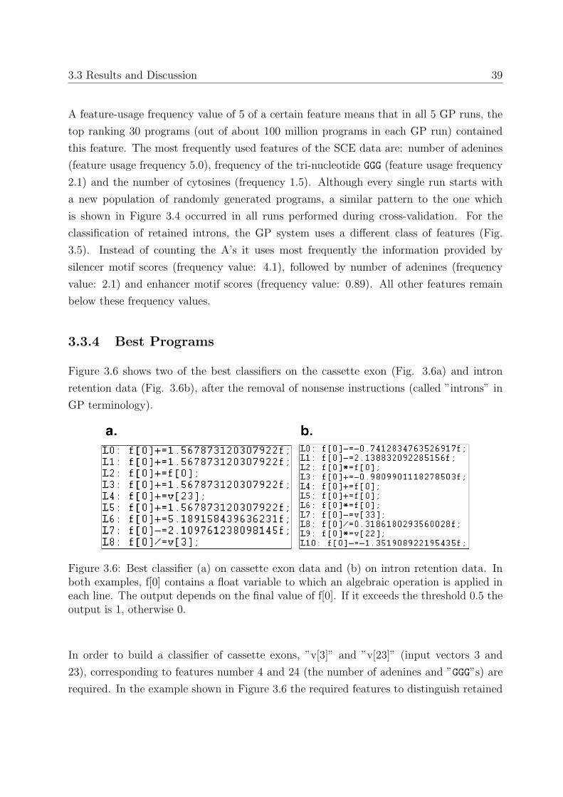
3.3 Results and Discussion 39
A feature-usage frequency value of 5 of a certain feature means that in all 5 GP runs, the
top ranking 30 programs (out of about 100 million programs in each GP run) contained
this feature. The most frequently used features of the SCE data are: number of adenines
(feature usage frequency 5.0), frequency of the tri-nucleotide GGG (feature usage frequency
2.1) and the number of cytosines (frequency 1.5). Although every single run starts with
a new population of randomly generated programs, a similar pattern to the one which
is shown in Figure 3.4 occurred in all runs performed during cross-validation. For the
classification of retained introns, the GP system uses a different class of features (Fig.
3.5). Instead of counting the A’s it uses most frequently the information provided by
silencer motif scores (frequency value: 4.1), followed by number of adenines (frequency
value: 2.1) and enhancer motif scores (frequency value: 0.89). All other features remain
below these frequency values.
3.3.4 Best Programs
Figure 3.6 shows two of the best classifiers on the cassette exon (Fig. 3.6a) and intron
retention data (Fig. 3.6b), after the removal of nonsense instructions (called ”introns” in
GP terminology).
Figure 3.6: Best classifier (a) on cassette exon data and (b) on intron retention data. Inboth examples, f[0] contains a float variable to which an algebraic operation is applied ineach line. The output depends on the final value of f[0]. If it exceeds the threshold 0.5 theoutput is 1, otherwise 0.
In order to build a classifier of cassette exons, ”v[3]” and ”v[23]” (input vectors 3 and
23), corresponding to features number 4 and 24 (the number of adenines and ”GGG”s) are
required. In the example shown in Figure 3.6 the required features to distinguish retained

40 3 Prediction of alternative splicing variants in human
introns are the number of ”GC” dinucleotides divided by intron-length and the scores for
exonic splicing silencers (Feature 34)(Gooding et al. 2006). The programs are read from
top to bottom and the result is compared to the threshold value. If the result is below 0.5
the classifier’s output is ”constitutive”, otherwise it is ”alternative”.
3.3.5 Improving hit rates on a more restrictive data set
In order to more critically evaluate our strategy, we have used the supplementary data set
from Sorek et al. (Sorek et al. 2004) to test our approach. We took their 453 cassette
exons as positive examples (class I) for the training set. As negative examples (class 0)
we took the constitutively spliced exons from the post-processed AltSplice data set (see
Methods) and required that the exon length was divisible by three (resulting in 10,774
exons) such that the data were in this repect compatible with the data set from Sorek
et al. Training of the GP system requires an attribution of weights to class 0 and class
I hits to account for the grossly different sizes of class 0 and class I data sets. As test
data set we considered 309 exons with missing EST support but which were predicted as
alternative by Sorek et al. We then have performed two different experiments. The goal of
the first experiment was to analyze the set of 309 exons under conditions of high specificity.
Parameters of the GP system were therefore adjusted to find constitutively spliced exons
rather than SCEs. This required to increase the weight for class 0 hits. After training,
on average only 50.6% of SCEs were classified correctly, but the correct detection rate of
constitutive exons increased to 87.6% (i.e. higher specificity). Under these conditions,
the top ranking features were ”length of exon” with a feature usage frequency value of
3.0 and ”number of adenines” with a frequency value of 2.2. All other features remained
below a frequency value of 1.0. Applying the classifiers to the set of 309 exons, classified
as alternative by Sorek et al., only 32.5% of them, 18% less than expected, were classified
as alternative by the GP system. In the second experiment parameters were adjusted to
raise the sensitivity, in a trade-off for specificity. After training, average sensitivity was
76.2% and average specificity was 53.5%. The top ranking feature was now ”frequency of
the tetra-nucleotide TGGA” with a frequency value of 3.0. The frequency value of all other
features remained below 1.0. Applying the classifiers to the set of 309 exons, 65.5% of them
were classified as alternative, almost 11% less than expected. As a conclusion of these two
experiments, we note that the classification of the 309 ”new” alternative exons by Sorek
et al. [16] differs from the results of our analysis, where roughly 35% of them are classified

3.3 Results and Discussion 41
as constitutive. Taking into account that the GP system on average misses 24% of the
true alternative exons, the question remains whether the 11% of supposedly misclassified
exons are truly alternative exons or not. It will be interesting to investigate the reason for
this discrepancy in more detail once sufficient EST data become available. We observed
for each of the two experiments a similar pattern of feature usage in the different GP runs.
However, as the task changed in the second experiment, the pattern of feature usage also
changed compared to the first experiment. It is interesting to note that GP can be used
for the identification and selection of important features not only for cassette exons and
intron retention splice variants but also for all other splice variants but which have not
been considered in this work.
3.3.6 Testing the robustness of the retained intron dataset, based
on experimentally validated data
Some cases of intron retention may be artefacts and the result of only partially completed
splicing. It is hard to gather experimental evidence for such cases. In order to ensure
that the prediction accuracies presented on the SIR data are not confounded by artefac-
tual effects of the AltSplice dataset, we tested the GP system on 17 conserved introns,
embedded in coding sequence and known to be alternatively retained (Ohler et al. 2005).
For training, we used the AltSplice dataset of 2,456 SIR introns and the same number of
constitutively spliced introns, randomly selected from the dataset of 21,677 constitutive
introns. This step was repeated ten times resulting in ten different training sets. The sep-
aration into two datasets of the same size eliminates the necessity of differential weighting
of the datasets. In 7 of the 10 experiments all 17 retained introns were classified correctly;
only 3 times one intron was misclassified, resulting in a hitrate of 98,2%. The best team
(see Methods) solution performed even better: only one intron was misclassified resulting
in a hitrate of 99.4%. Both results on experimental data are far above the average hitrate
on AltSplice data (92.1%, see Table 3.2), indicating that the system performs well despite
the fuzziness of the data.
Chapter 4
Critical evaluation of alternative
splicing prediction
In the previous chapter, we introduced a GP approach for the prediction of alternative
splicing variants in human. Providing the basic feature matrix, shown in Table 3.1, high
prediction accuracies could be achieved on the SIR dataset, 85%; in contrast the prediction
accuracies on skipped exons remained below 60%. We found that different features were
used for the classification of the two different splicing variants (see Figures 3.4 and 3.5).
Thereby the most frequently used feature for the SIR classification was the silencer score,
which might be explained by the observation that retained introns appeared to harbor
”exon properties” and were clearly distinguishable from constitutive introns, regarding
this feature (Figure 3.3). However, why the feature A was important for classification of
constitutive exons, and also the reason for the big discrepancy in the prediction accuracies
between SIR and SCE, could not be explained.
The following chapter addresses these open questions. We start with an attempt to increase
the prediction accuracies on exon data by investigating and adding new features to the
feature matrix. The focus is initially on A-related-features, therefore we investigate A-
stretches and the nucleotide compositions of ESE found in the different sets of exons.
Although we find that the most prevalent ESEs in exons tend to be especially A-rich in case
of constitutive exons, we are unable to derive a general rule and to increase the prediction
accuracies. Therefore we critically question the hypothesis that sequence composition is
responsible for the good recognition of intron retention events. To eliminate the influent
feature ”length”, we analyze a subset of short constitutive introns and compare them with
retained introns. We compare our results with a state of the art SVM approach. As a

4.1 Additional features for classification of skipped exons 43
final consideration, we reveal how a failure to adopt an unified terminology within the
greater splicing community can lead to inconsistencies in data generation, handling and
comparison. We provide a more generalized and objective approach to label the data in
future.
4.1 Additional features for classification of skipped
exons
While the GP-system was able to distinguish between retained- and constitutively spliced
introns with an accuracy of 85%, the prediction accuracies on the skipped exons dataset
remained below 60%. Despite the variety of the features provided to the GP-system, it
remained also unclear why the total amount of ”Adenine” within the exons was always
preferred to classify the exons, over any other feature. The following section summarizes the
most promising attempts to explore further features involved in constitutive and alternative
splicing.
4.1.1 A-stretches
One of the results above was that, in order to classify between skipped and constitutive
exons, the GP-system used the total amount of Adenine. Thereby it did not play any
role how the ”A”s were distributed across the exons. In order to explore the A-feature,
we asked the question if the A-bases are distributed in clusters or rather randomly, and
if there are spatial differences between the A-distributions in constitutive versus skipped
exons, in a way that specific proteins might be able to bind better in one of the two exon
classes.
In order to perform this analysis we transformed every exon sequence into a form containing
only the length of the A-stretches and their distances to one another. e.g. an exon of the
sequence gcaccgtaaccgaaaaa, would be transformed into: A1-d4-A2-d3-A5. ”A”s in this
example mark the lengths of the A-stretches, whereas ”d”s indicate the distances. We
applied this method to the dataset of all skipped- and constitutive exons, as well as to
their shuffled counterparts. The summarized results are shown in Table 4.1. The complete
length and distance tables can be found in the supplement section (Tables 8.2 and 8.3).
In case of SCE, 74% of all ”A”s were ”singletons”, 18% occurred as dinucleotides, and 5%

44 4 Critical evaluation of alternative splicing prediction
Table 4.1: A-stretches
A-Stretches SCE SCE-Shuffled (1Run) Const Const-Shuffled (1Run)A1 0.7417 0.7365 0.7217 0.7217A2 0.1811 0.1910 0.1932 0.1977A3 0.0533 0.0510 0.0579 0.0563d1 0.3200 0.3142 0.3259 0.3214d2 0.1928 0.1853 0.2035 0.1926d3 0.1176 0.1305 0.1185 0.1348d4 0.0894 0.0953 0.0907 0.0957d5 0.0734 0.0693 0.0734 0.0690
occurred as A-triplets. The distance between two ”A”s was in 32% of all cases only one
base pair. This value was not elevated compared to that found in randomized sequences.
Comparing the results of SCE with shuffled data as well as with constitutive data, no
significant differences could be observed, suggesting that this feature might not be of
fundamental importance.
4.1.2 Composition of Exonic Splicing Enhancers
We showed that alternative exons do not differ from constitutive exons regarding the
densities of exonic splicing enhancers (Figure 3.3). Here, we addressed the question if
the nucleotide compositions of ESEs within constitutive exons are different compared to
skipped exons, e.g. if the enhancer elements contained within constitutive exons tend to
be A-rich.
For each exon, we extracted and analyzed the nucleotide compositions of the ESEs con-
tained in the exon. This information was used to generate a new feature matrix containing
four features for each nucleotide, as well as a feature matrix containing the trinucleotides
information. Furthermore we were also interested in finding out, if the most frequently
used motifs differ between the two datasets. The complete lists of the 40 most abundant
ESE words can be found in the appendix part of the thesis (Tables 8.5 and 8.4), the top
five words found in the two classes of exons, can however be found in Table 4.2.
It is interesting to note that the top five words within the constitutive dataset are enriched
in ”A”s, whereas skipped exons are rather depleted regarding this feature. The constitutive
dataset consists of ”GAA” repeats, in case of SCE, ”CCT” or ”CT” could be localized in each
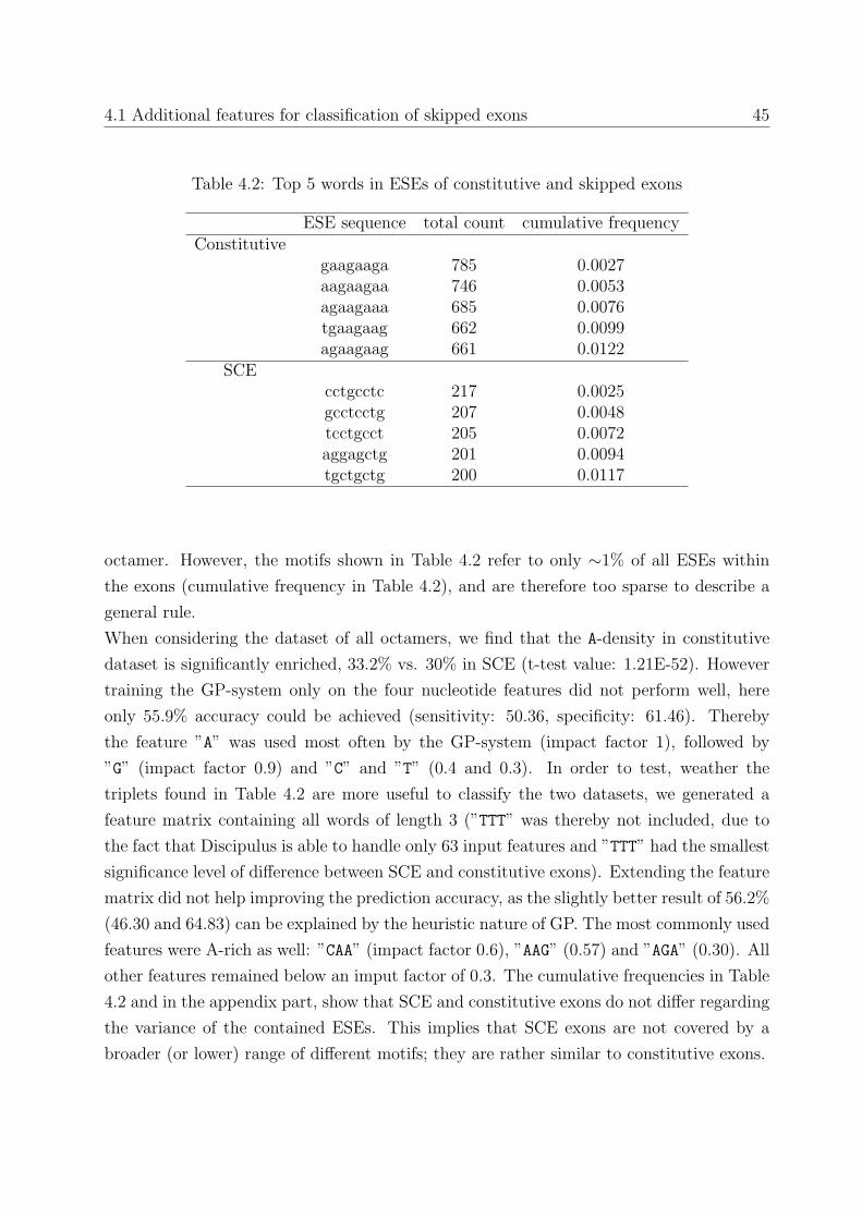
4.1 Additional features for classification of skipped exons 45
Table 4.2: Top 5 words in ESEs of constitutive and skipped exons
ESE sequence total count cumulative frequencyConstitutive
gaagaaga 785 0.0027aagaagaa 746 0.0053agaagaaa 685 0.0076tgaagaag 662 0.0099agaagaag 661 0.0122
SCEcctgcctc 217 0.0025gcctcctg 207 0.0048tcctgcct 205 0.0072aggagctg 201 0.0094tgctgctg 200 0.0117
octamer. However, the motifs shown in Table 4.2 refer to only ∼1% of all ESEs within
the exons (cumulative frequency in Table 4.2), and are therefore too sparse to describe a
general rule.
When considering the dataset of all octamers, we find that the A-density in constitutive
dataset is significantly enriched, 33.2% vs. 30% in SCE (t-test value: 1.21E-52). However
training the GP-system only on the four nucleotide features did not perform well, here
only 55.9% accuracy could be achieved (sensitivity: 50.36, specificity: 61.46). Thereby
the feature ”A” was used most often by the GP-system (impact factor 1), followed by
”G” (impact factor 0.9) and ”C” and ”T” (0.4 and 0.3). In order to test, weather the
triplets found in Table 4.2 are more useful to classify the two datasets, we generated a
feature matrix containing all words of length 3 (”TTT” was thereby not included, due to
the fact that Discipulus is able to handle only 63 input features and ”TTT” had the smallest
significance level of difference between SCE and constitutive exons). Extending the feature
matrix did not help improving the prediction accuracy, as the slightly better result of 56.2%
(46.30 and 64.83) can be explained by the heuristic nature of GP. The most commonly used
features were A-rich as well: ”CAA” (impact factor 0.6), ”AAG” (0.57) and ”AGA” (0.30). All
other features remained below an imput factor of 0.3. The cumulative frequencies in Table
4.2 and in the appendix part, show that SCE and constitutive exons do not differ regarding
the variance of the contained ESEs. This implies that SCE exons are not covered by a
broader (or lower) range of different motifs; they are rather similar to constitutive exons.

46 4 Critical evaluation of alternative splicing prediction
4.1.3 Do ESE cluster?
The top five words in Table 4.2 overlap, due to the short repeated sequences contained, to
a great extent. In order to investigate, if ESE tend to cluster in general and if there are
differences in skipped vs. constitutive data, we calculated the extent by which each base
within an exon is covered by an ESE octamer. In case the octamers are not overlapping
at all, the coverage value is 1, whereas the maximum value that can be reached is 8. In
this case a stretch of eight octamers (or more) are positioned next to each other, with a
distance of 1 nucleotide. Both SCE and constitutive exons have a coverage of 0 in 70% of
all cases, thus only 30% of the base pairs are covered by an ESE element. Figure 4.1 shows
the distribution of the coverage values from 1 to 8.
Figure 4.1: ”Frequency Spectrum” of ESEs overlaps per nucleotide within SCE and con-stitutive exons. The two datasets do not show differences.
Both distributions are indistinguishably similar, revealing that this feature cannot be used
to improve the classification accuracy. Nevertheless it is interesting to note that real exons
differ from synthetic ones (introduced in chapter 5) regarding this feature, in so far as real
exons are decreased in coverage value 1 but increased in coverage classes 2-8, indicating
that clustering of ESEs is more likely to be observed than expected by chance (Appendix
Material).

4.1 Additional features for classification of skipped exons 47
4.1.4 Exons with intronic properties
We showed that retained introns appear to harbor ”exon properties” (3.3). In order to
explore if cassette exons bear some sequence properties which can also be found in introns,
we compared dinucleotide frequencies of exons with the flanking up- and downstream exons
as well as with up- and downstream introns. Thereby we defined
”exon properties” as: α:= 2·exonupstream exon+downstream exon
and
”intron properties” as: β:= 2·exonupstream intron+downstream intron
.
Comparing the α and β values of SCE and constitutive exons did not give a new hint for
a better partition of the two datasets. We therefore tried another approach, considering
only dinucleotides that were separating (in terms of densities) constitutive exons from
introns, and positioning a skipped exon closer to introns than to exons (see Appendix
Figure 8.1, ”AG” dinucleotide). Then we extended the specific dinucleotide and formed
8 different triplets by adding the four possible nucleotides either to the beginning or to
the end. We analyzed the resulting triplets (Appendix Figure 8.2) and extended them
to form 4mers, by proceeding as described before (Appendix Figure 8.3). Finally we
constructed a feature matrix consisting of the features ”length”, ”AG”, ”AT”, ”AGT”, ”GAGT”
and ”AGTG” (measured in exons and flanking introns). With a prediction accuracy of
56.83% (sensitivity: 44.65, specificity: 69.00 ), the results remained below the original
feature matrix, suggesting that SCE exons do not carry intronic properties differently to
constitutive exons.
4.1.5 Transformations from ESE to ESS
Many known diseases are caused by destruction/creation of ESEs and ESSs (Chapter
2.1.2). In order to test the ”robustness” of the system, we investigated the minimum
number of mutations that are required to turn an ESE into ESS (and vice versa) and tested
weather SCE might consist of ESEs which are easier convertible into ESS. Furthermore we
calculated the average distance (number of mismatches between two octamers) between
each octamer within SCE, constitutive, and pseudo exons, to the list of all ESE- and ESS
octamers.
Figure 4.2 shows that the minimum number of mutations to turn an ESE into an ESS
is between 2 and 3. The skipped exons contain ESEs which are similarly transformable

48 4 Critical evaluation of alternative splicing prediction
Figure 4.2: Minimum amount of mutations for ESE to ESS transformations
in comparison to constitutive exons. Appendix Figure 8.4 shows the distribution of the
distances from each octamer to the datasets of all ESE and ESS motifs. For SCE and
constitutive exons the peak is around value 6, which is exactly what one would except by
considering the distance of two octamers by chance:∑8
k=1 (8k)·3k
48 =6.
4.1.6 Separating the datasets according to their inclusion levels
So far we classified constitutive vs. skipped exons. However, the separation of the data
into two classes might be outdated as the splicing vocabulary is in change (a discussion
about this issue can be found in the next chapter). As mentioned above (chapter 2.1.4),
other authors subdivide their data into three or five classes (Modrek and Lee 2003;
Xing and Lee 2006; Zhang and Chasin 2006). In order to ensure that the lack of differ-
ences between skipped and constitutive exons in our dataset, is not caused due to focussing
on outdated terms, we subdivided our dataset of exons into seven classes, according to their
inclusion levels. The inclusion levels were calculated with a program provided by E.Eyras
(Plass and Eyras 2006) based on EST and cDNA data from human genome release 18,
March 2006, which we downloaded from the UCSC homepage (NN 2008b). The separation
of the seven inclusion level classes is as follows:

4.1 Additional features for classification of skipped exons 49
• Class 1: Always excluded
• Class 2: Included in up to 10% of all transcripts
• Class 3: Included in more than 10% and up to 40% of all transcripts
• Class 4: Included in 40%-60% of all transcripts
• Class 5: Included in 60%-90% of all transcripts
• Class 6: Included in more than 90% of all transcripts
• Class 7: Always included
Furthermore we improved the feature-matrix by including additional exonic splicing en-
hancers and -silencers features. In addition to the octamer ESE- and ESS-sequences pro-
vided by Zhang and Chasin (Zhang et al. 2005)(Features 32 and 34 of the basic Feature-
Matrix) we also analyzed the collection of ESE and ESS hexamer sequences provided by
Fairbrother and Burge (Fairbrother et al. 2002). A description of how the two datasets
were generated and about their differences can be found in chapter 2.1.3. This chapter
also introduces the SELEX method, by which the SR-protein position weight matrices
were built(Liu et al. 1998). We downloaded the four matrices for SRp55, SRp40, SC35
and SF2ASF and generated an own list of SR protein words by considering the threshold
values provided with the matrices. Both, the matrices and their corresponding threshold
values, used for this study, can be found in Appendix Figure 8.5.
For each of the lists of words, we calculated the percentage of the nucleotides within an
exon that were covered by the motifs with respect to their overlap. E.g., an exon of length
100 containing two ESE octamers at positions 1 and 50 has an ESE coverage of 16%,
whereas two octamers at positions 1 and 2 lead to an ESE coverage of 9%. The results are
shown in Figure 4.3. An overview about the percentage of the overlapping words, between
the different sets of motifs, can be found in Chapter 5.3.5.
An intuitive expectation prior to the experiment was that an increasing amount of exonic
splicing enhancers should lead to an increasing inclusion of a certain exon, whereas an
increasing amount of exonic splicing silencers would lead to a depletion of transcripts
containing the exon, thus to lower inclusion levels. In contrast to our expectations, Figure
4.3 does not support this trend, it rather shows no appreciable differences between any of
the classes. From these results, we can conclude two things. The separation of alternatively

50 4 Critical evaluation of alternative splicing prediction
Figure 4.3: Separation of the data according to their inclusion levels. The densities of ESEand ESS motifs are not changing throughout the groups of different inclusion levels.
spliced exons into seven inclusion level classes does not provide any higher resolution than
if there are only two such classes. Secondly, and more importantly, these results question
the current computational status quo: that the key to alternative splicing prediction can
be attributable to DNA sequence alone.
4.2 Short constitutive introns (short constI)
The results presented above have demonstrated two very important points. SIR introns
are easily and precisely classifiable by GP methods, whereas classification accuracy (60%)
for skipped exons could not be improved, despite incorporation of many new strategies and
approaches. We critically questioned the hypothesis that sequence composition was the key
factor contributing to the huge discrepancy between the prediction accuracies for retained
introns (SIR) (85%) versus cassette exons (SCE) (60%). We found that the length of the
sequences strongly influenced prediction accuracies between the two classes. We showed in
Figure 3.1 that SCE exons are ∼8% shorter than constitutive exons; but that SIR introns

4.2 Short constitutive introns (short constI) 51
are shorter than constitutive introns by an order of magnitude. A way to eliminate the
bias on length was to choose a subset from the original dataset of constitutive introns, with
equal average lengths to SIR. We have chosen only introns shorter than 534bp, resulting in
4032 constitutive introns (out of 33316), with similar length distributions to SIR (Result
of TTest: 0.995), shown in Figure 4.4.
Figure 4.4: The length distributions of SIRs and short constitutive introns are similar
We used the classifier produced based upon the original feature matrix (shown in Figure
3.6) to test the short constI data. If the hypothesis was true, that solely sequence compo-
sition was responsible for the accuracy rates on the SIR data, then the short constI should
still be classified as constitutive. We found that ∼90% of all short constI were misclas-
sified as ”alternative”. The classifier built upon all introns was obviously not well suited
to detect short constI, therefore we built a new classifier explicitly designed to distinguish
between SIR and short constI. The prediction accuracy dropped down to ∼64% (sensitiv-
ity:50.77, specificity:76.79) indicating that there is still more sequence signal to be found
in comparison with skipped exons, but not as much as initially expected.

52 4 Critical evaluation of alternative splicing prediction
4.3 Comparing our results with a Support Vector Ma-
chine approach
Raetsch and colleagues designed a SVM kernel to classify alternative exons in C.elegans.
In contrast to any published approach available, their approach did not require any infor-
mation of the conservation level (Ratsch et al. 2005). The resulting SVM-based classifier
achieved a sensitivity of 48.5% at a specificity of 99% in C.elegans. Unfortunately they did
not report how the system performed on human genetic data, therefore the results could
not be compared straightforwardly. In order to find out, if the SVM performs better or
worse than our GP-System, we used an online version of the SVM (Raetsch et al. 2008)
and encompassed our feature matrix to it. Thereby we tested the three different kernels
available: Linear, Polynomial and Gaussian. For each of the kernels different configurations
were tested, in order to find the optimal settings for the SVM regularization parameter C,
and the kernel parameters. Additionally, we used the ”SVM Model Selection” tool, pro-
vided within the SVM package, to find the best combination of SVM hyper-parameters.
The best accuracy results on our data were achieved with the following settings:
• Kernel: Polynomial
• SVM regularization parameter C: 1.0
• The degree of the Polynomial Kernel: 2
In contrast to Discipulus, here we had to separate the datasets into equal sizes. We chose
a random subset of 7323 constitutive exons, out of the total amount of 27224 constitutive
exons. In order to have completely comparable results, we encompassed the newly sepa-
rated datasets also to the GP-system Discipulus. The comparison of the results, shown
in Table 4.3, indicates that the two different Machine Learning approaches are similar in
spirit of motif recognition.
Table 4.3: GP vs. SVM
Method sensitivity specificity (sen+spe)/2SVM 63.46 53.65 58.55
GP 54.16 64.15 59.16

4.4 General remarks on the terminology of splicing 53
4.4 General remarks on the terminology of splicing
Until a few years ago the definitions of constitutive and alternative exons were well defined:
”Constitutive exons are found in every transcript of a gene whereas alternative exons are
absent in at least one transcript that would have been long enough to contain it.” Boue et
al. (Boue et al. 2003). However, with increasing amounts of EST and cDNA data (Figure
2.3), the big picture becomes more blurry. There are ongoing debates about how many of
these predicted splice variants are in fact functional and how many are rather the result of
aberrant splicing (or ’noise’) (Sorek et al. 2004; McGuire et al. 2008). The effect might
be demonstrated in following experiment. In order to critically control if our dataset of
constitutive exons from year 2003 is still considered to be constitutive, we tested the data
with 3 different approaches:
Figure 4.5: Testing the validation status of the AltSplice constitutive exon dataset withdifferent approaches leads to different results
1. The EST clustering method described in (Plass and Eyras 2006) showed that 86%
of ”constitutive” exons had exclusion levels higher than 10%, confirming only 14% of the
exons as constitutive (Figure 4.5 a).
2. By using the Ensembl Biomart Tool (Birney et al. 2006), 88.5% of our constitutive
exons were confirmed, however 49.5% of the skipped exons were annotated as ”constitu-
tive” (Figure 4.5 b).
3. We performed a spliced alignment with the whole genomic area including the up- and
downstream exons and introns. We used the program ”GenomeThreader” which calculates
spliced alignments and creates quality scores for exon similarity and donor- and acceptor
splice sites. The first approach used only cDNA information without cancerous tissue.
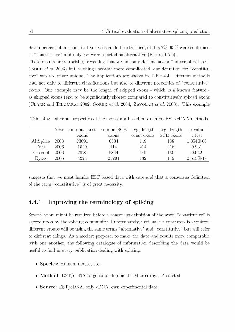
54 4 Critical evaluation of alternative splicing prediction
Seven percent of our constitutive exons could be identified, of this 7%, 93% were confirmed
as ”constitutive” and only 7% were rejected as alternative (Figure 4.5 c).
These results are surprising, revealing that we not only do not have a ”universal dataset”
(Boue et al. 2003) but as things became more complicated, our definition for ”constitu-
tive” was no longer unique. The implications are shown in Table 4.4. Different methods
lead not only to different classifications but also to different properties of ”constitutive”
exons. One example may be the length of skipped exons - which is a known feature -
as skipped exons tend to be significantly shorter compared to constitutively spliced exons
(Clark and Thanaraj 2002; Sorek et al. 2004; Zavolan et al. 2003). This example
Table 4.4: Different properties of the exon data based on different EST/cDNA methods
Year amount const amount SCE avg. length avg. length p-valueexons exons const exons SCE exons t-test
AltSplice 2003 23091 6334 149 138 1.854E-06Fritz 2006 1520 114 214 216 0.931
Ensembl 2006 23581 5844 145 150 0.052Eyras 2006 4224 25201 132 149 2.515E-19
suggests that we must handle EST based data with care and that a consensus definition
of the term ”constitutive” is of great necessity.
4.4.1 Improving the terminology of splicing
Several years might be required before a consensus definition of the word, ”constitutive” is
agreed upon by the splicing community. Unfortunately, until such a consensus is acquired,
different groups will be using the same terms ”alternative” and ”constitutive” but will refer
to different things. As a modest proposal to make the data and results more comparable
with one another, the following catalogue of information describing the data would be
useful to find in every publication dealing with splicing.
• Species: Human, mouse, etc.
• Method: EST/cDNA to genome alignments, Microarrays, Predicted
• Source: EST/cDNA, only cDNA, own experimental data
4.5 Conclusions 55
• Conservation: Are the exons conserved between human and mouse (or another
species)?
• Protein coding: Are the exons limited to protein coding only, or are also UTR
exons considered?
• Frame preserving: Are the exons required to be divisible by 3?
• Stop codon: Are in frame stop codons allowed?
• Exon rank in transcript: Are the exons limited to middle exons only, or are also
first and last exons considered?
• EST-tissue: Are ESTs from cancer, cell-lines and tumor tissues allowed?
• Constitutive: How many contradicting transcripts are allowed? 0? 2 ESTs, 1
cDNA? 1%?
• Special issues: E.g. Conservation of the same splice pattern between two species,
etc.
4.5 Conclusions
In the first part of this chapter, we tried to increase the prediction accuracies on SCE
data, by investigating further features, not contained in the original feature matrix. We
started focussing on A-related features, since the GP system preferred the A-feature over
any other feature. Although the prediction accuracy could not be further increased, we
could show that the most abundant exonic splicing enhancers, found in constitutive exons,
are significantly enriched in ”A”s. This is a feature which has not been reported elsewhere
before. Comparing SIRs with short constI decreases the initial accuracy of ∼85% to ∼64%,
suggesting that intron length is more important than sequence composition. We compare
our results on SCE data with a state of the art SVM approach, and find out that the differ-
ence between both methods is small. The GP-system achieves a slightly better prediction
accuracy of 59.16% (vs. 58.55% in SVM), suggesting that the poor prediction accuracies
do not originate from choosing a wrong machine learning method, but they originate due
to similar signals and sequence properties of SCE and constitutive exons. Furthermore we
revealed inconsistencies with data descriptions and handling between different groups, and
provide a more generalized and objective approach to label the data in future.

Chapter 5
Modeling the exons
5.1 Introduction
Generating a dataset of synthetic exons (s.exons)
In order to compare specific properties of real vs. random exons, previous ap-
proaches have generated random exons by shuffling the exonic sequence of real exons
(Plass and Eyras 2006). However, shuffling the sequence destroys the information, e.g.
for splicing factor binding sites, and decreases the densities of cis-regulatory motifs, such as
Exonic Splicing Enhancers (ESE) which are essential for a proper splicing. Thus, shuffling
the sequences does not lead to ”random exons” but it rather results in sequences with a
lack of exonic properties. Here we generate sequences in a way that they resemble real
exons by integrating sequence properties learned from real constitutive exons. The goal
is to learn the rules of nature of how exons are constructed, leading to a generation of a
new dataset of ”synthetic exons” which will hardly be distinguishable from real exons by
any Machine Learning System. In contrast to previous chapters, this time the objective
function of the GP-system is antipodal, implying that good approximation of real exons
result in bad prediction accuracies.
To generate synthetic exons, we integrate our knowledge about real exons:
• The average length of constitutive exons is around 150bp (Figure 3.1)
• Exons have a higher GC-content compared to noncoding DNA (Figure 3.2).
• Exons contain ESE (Figure 3.3)
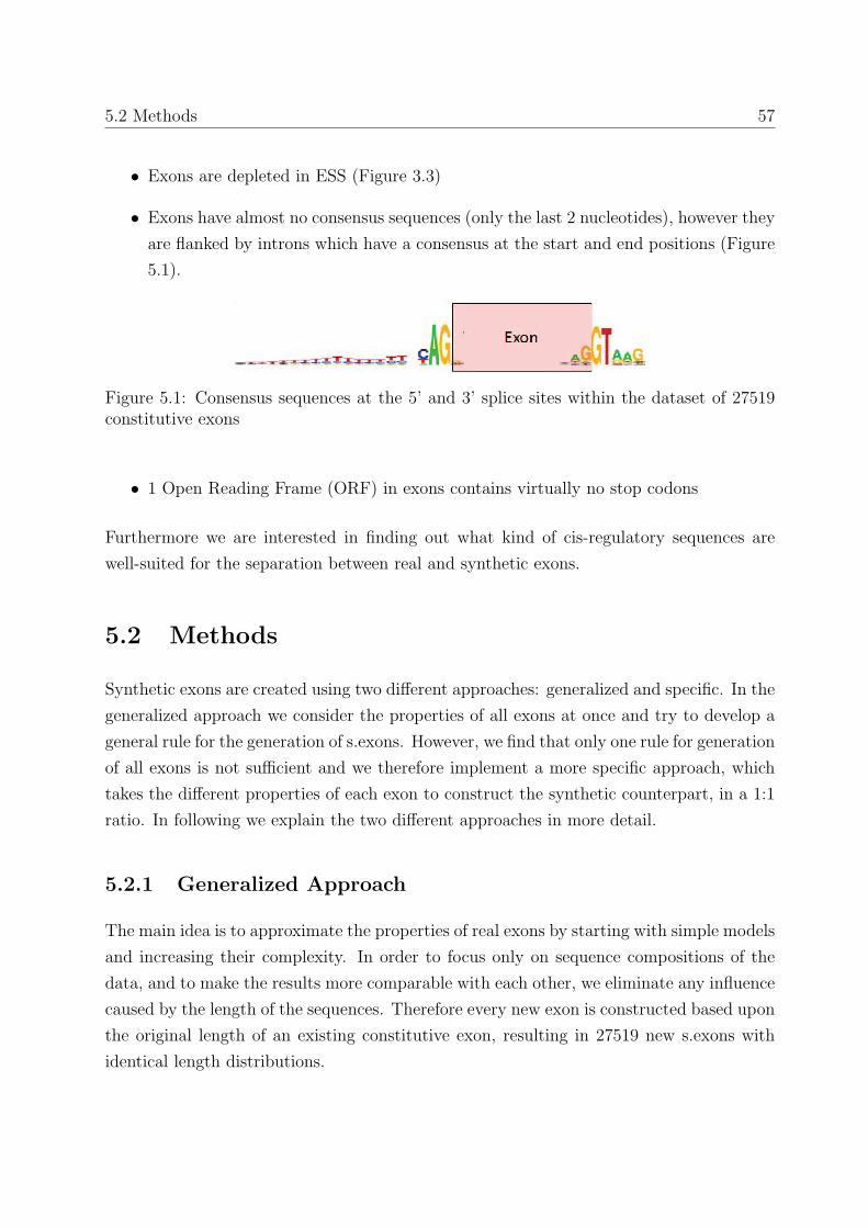
5.2 Methods 57
• Exons are depleted in ESS (Figure 3.3)
• Exons have almost no consensus sequences (only the last 2 nucleotides), however they
are flanked by introns which have a consensus at the start and end positions (Figure
5.1).
Figure 5.1: Consensus sequences at the 5’ and 3’ splice sites within the dataset of 27519constitutive exons
• 1 Open Reading Frame (ORF) in exons contains virtually no stop codons
Furthermore we are interested in finding out what kind of cis-regulatory sequences are
well-suited for the separation between real and synthetic exons.
5.2 Methods
Synthetic exons are created using two different approaches: generalized and specific. In the
generalized approach we consider the properties of all exons at once and try to develop a
general rule for the generation of s.exons. However, we find that only one rule for generation
of all exons is not sufficient and we therefore implement a more specific approach, which
takes the different properties of each exon to construct the synthetic counterpart, in a 1:1
ratio. In following we explain the two different approaches in more detail.
5.2.1 Generalized Approach
The main idea is to approximate the properties of real exons by starting with simple models
and increasing their complexity. In order to focus only on sequence compositions of the
data, and to make the results more comparable with each other, we eliminate any influence
caused by the length of the sequences. Therefore every new exon is constructed based upon
the original length of an existing constitutive exon, resulting in 27519 new s.exons with
identical length distributions.

58 5 Modeling the exons
model 1
”Model 1” s.exons are generated by concatenating the nucleotides A,C,G, and T. Thereby,
every nucleotide has the same probability of 25% for being chosen. The process of con-
catenation stops, when the length of the first real exon in the list of all constitutive exons
is reached. We then proceed with the generation of a second s.exon by taking the length
of the second exon and continuing in the same way as described above, until the list of all
27519 is processed, and 27519 new ”model 1” s.exons are generated.
model 2
In order to generate ”model 2” s.exons, the nucleotide frequencies of real constitutive
exons are measured and saved into a matrix containing the four frequency values: A:
27.4%, C:24.2%, G:25.4%, and T: 23.0%. New s.exons are constructed by concatenating the
nucleotides according to the probabilities contained in the matrix.
model 3
To generate ”model 3” s.exons, we measure dinucleotide frequencies of constitutive exons.
We save the frequencies of all 16 dinucleotides into a matrix, which is then used to determine
the probability of a certain dinucleotide to be concatenated.
model 4
”model 4” is similar to model3, only improved by including the consensus dinucleotide
sequences at the end of exons.
model 5
Similar in spirit to the models before, here we count the frequencies of all 64 trinucleotides
detected in constitutive exons, and generate the s.exons based upon them.
adjusted model 5 Based upon the 27519 sequences generated by model 5, the adjusted
model chooses only sequences which resemble the ESE coverage of real exons. The se-
quences with a lower ESE coverage are rejected, resulting in 14159 synthetic exons. The
ESE distributions are shown in (Appendix Figure 8.9).
model 6
The frequencies of all 4096 hexamers, detected in constitutive exons are used to generate
the synthetic dataset. The consensus sequences are included at the end of exons.
model 7
The disadvantage of previous models is that although the n-mer frequencies are initially
taken from real exons, by concatenating the n-mers, each junction generates n-1 new n-
mers (e.g. aaa and ttt generate the triplets aat and att after concatenation). In some

5.2 Methods 59
cases also stop codons might be generated by combining two n-mers, which do not belong
together. One consequence is e.g. the 25fold higher observation of stop codons within
the s.exons (Figure 5.5). In order to improve the exonic properties, the new model is
constructed based upon triplet-transition-probabilities. For every possible triplet from aaa
to ttt, the probabilities for the flanking 3-mer are measured within the constitutive exon.
The s.exon is generated by starting with a random 3-mer (according to overall starting
3-mer frequencies), and concatenating the next one based upon the probability value in
the triplet-transition-probabilities-matrix.
model 8
To eliminate the high stop codon densities (shown in Figure 5.5), the correct ORF has been
estimated in order not to take the entire set of triplet transition probabilities occurring in
an exon, but only the correct ones which do not introduce a stop codon.
5.2.2 Specific Approach
word length 1-10
Instead of taking the properties of all exons into consideration, real exons serve as templates
for new s.exons. Different models involve different lengths of n-mer words considered,
starting with a word length of 1 and increasing it to 10. The new exons are generated
based upon the frequencies of the specific words within the template exons. Taking a word
length of 1 e.g. resembles shuffling the exon by preserving a similar AGCT content, whereas
taking a word length of 10 preserves greater exonic blocks. The consensus dinucleotide
sequence was added at the last two positions of each s.exon.
reverse exons
Reverse exons were generated by reading the 5’→ 3’ exons in the 3’→ 5’ direction. The
reverse exons have a different feature matrix which is based upon all sixteen possible
dinucleotides.

60 5 Modeling the exons
5.3 Results
5.3.1 ESE - Densities
As mentioned above, one of the features in real exons is a specific content of ESEs. In
order to estimate how well this feature could be remodeled, we compared the densities of
ESEs (based upon Zhang and Chasin set of octamers (Zhang and Chasin 2004)) between
our new synthetic exons and the constitutive ones. Thereby we measured and plotted the
percentage of the nucleotides which are covered by an ESE motif. In case of real exons
(red bold line in Figure 5.2) in average 29.8% of the exonic sequence is covered by these
regulatory motifs. Whereas only 17.5% of random sequences, with the same GC content
(generated by model 2), contain these ESE motifs. As the complexity of the models
increases, also the distributions of the ESE densities resemble more and more those of
genuine exons (Figure 5.2). This result shows that by chance, even with a proper GC
content, the amount of these motifs is substantially lower for random sequences.
Figure 5.2: ESE-densities: an increased model complexity leads to a higher amount ofESEs

5.3 Results 61
Figure 5.3: ESE-densities on the specific dataset
In case of the generalized approach, the two models based upon triplet-transition proba-
bilities overlap the ESE density curves of real exons accurately (Figure 5.2 and Appendix
Figure 8.10). This property cannot be resembled within the specific approach which is
based solely on word counts (Figure 5.3).
5.3.2 ESE regulatory networks
Earlier, we investigated the densities of ESEs, and also the abundance of the most fre-
quently appearing ESEs (Chapter 4.4). Here, we asked the question if there is a co-
occurrence between certain ESEs, or if they rather appear independent from one another.
We were also interested in the distances between two different ESEs which co-occur to-
gether. To calculate the co-occurrence values of two ESEs, and their distances, we built a
NxN matrix, where N is the number of total ESEs (=2069). Each ESE was assigned an
unique number between 1 and 2069, as an identifier. For every exon, we identified all f
ESEs contained, and built all(
f2
)possible pairwise combinations between them. For each
two ESEs e1 and e2, we incremented the value in the upper triangle of the matrix at the
position [e1][e2], while the lower triangle of the matrix was used to save the average distance
between e1 and e2 at the position [e2][e1]. The main diagonal of the matrix remained 0,
62 5 Modeling the exons
since we were only interested into co-occurrences of different ESEs. Finally we compared
the results of real with simulated data. Table 5.2 shows the properties of the top 3 motifs
which co-occur with one another within constitutive exons, m2, m6, m7 s.exons, and SCE
exons. We find that distances for motifs which co-occur together are in 95% of all cases
below 8, implying that these motifs overlap in general (Table 5.2 ”average distance” and
”percentage of overlap”). In case of constitutive exons, 269 out of 27519 exons (0.98%)
contain the same co-occurring ESE motifs, with an average distance of 3 bp, and 96% of
them overlapping. This co-occurrence number is 7 times higher compared to m2 s.exons,
containing only a maximum number of 36 co-occurring motifs, and can partly be explained
by the fact that m2 contain in general less ESE motifs.
It is interesting to note that m7 s.exons and const exons contain similar motif-ids, each
of them containing the hexamer ”gaagaa”. The motif-ids between m2 s.exons and const
exons, do not overlap at all. The same is true between SCE and Const exons, but here also
the motifs are substantially different 5.2, as SCE have as the most abundant motif ”cct”
instead of ”gaa”. Analyzing the top 300 co-occurring motifs within constitutive exons and
comparing them with the top 100 motifs within the SCE data (here we consider less motifs
due to a smaller exon samplesize) reveals that the ”A”-nucleotide, is substantially enriched
between constitutive and SCE exons, but also in comparison to the overall frequency of ”A”
in all Chasin ESEs (here, the frequency of nucleotide ”A” is 29.9% in average, see chapter
5.3.5 for nucleotide compositions in Chasin ESE data). The nucleotide compositions of co-
occurring motifs are in case of constitute exons, A: 46.7%, C: 7.6%, G: 39.0% and T:6.7%;
and in case of SCE exons A: 40.9%, C: 9.6%, G: 41.6% and T:7.9% respectively. This result
indicates that an increased number of ”A”s increases at the same time the probability of
ESE-networks, as well as the probability of classifying a constitutive exon.
On large scale however, the differences shown in Table 5.2 cannot be manifested. Appendix
Figure 8.11 shows the co-occurrence networks of the top 300 motifs within const exons,
s.exons and the top 100 motifs within the SCE data, all bearing similar patterns. The
distance distributions of the top 300 motifs within constitutive exons and m2 s.exons, are
shown in Appendix Figure 8.12, indicating that the high rates of the overlapping between
two ESEs, is expected by chance.

5.3 Results 63
Tab
le5.
1:Top
3E
SE
mot
ifs
co-o
ccurr
ing
toge
ther
num
ber
ofper
centa
geex
ons
conta
inin
gav
erag
eof
over
lap
dat
aset
the
2E
SE
sid
e 1id
e 2se
quen
cee 1
sequen
cee 2
dis
tance
of2
ESE
sC
onst
269
8912
16aa
gaag
aaga
agaa
ga3.
0396
%27
519
249
8936
4aa
gaag
aaag
aaga
aa5.
4594
%ex
ons
249
366
1216
agaa
gaag
gaag
aaga
2.48
96%
m2
3636
513
64ag
aaga
acga
gaag
aa1
100%
2751
935
9512
17aa
gaag
cgga
agaa
gc1
100%
s.ex
ons
3297
715
89cg
gaga
aagg
agaa
aa5.
8497
%m
698
8912
16aa
gaag
aaga
agaa
ga4.
8595
%27
519
9815
9319
85gg
agaa
gatg
gaga
ag1.
9399
%s.
exon
s91
1117
1985
ctgg
agaa
tgga
gaag
3.46
97%
m7
204
8912
16aa
gaag
aaga
agaa
ga1.
6999
%27
519
203
8936
6aa
gaag
aaag
aaga
ag2.
0799
%s.
exon
s19
436
612
16ag
aaga
agga
agaa
ga2.
4698
%SC
E12
689
918
07cc
tgcc
tctc
ctgc
ct1.
3699
%96
4171
538
1425
agga
gctg
gagg
agct
3.24
99%
exon
s69
538
1606
agga
gctg
ggag
ctgg
6.49
93%

64 5 Modeling the exons
5.3.3 ESS - Densities
In contrast to ESE-, the ESS-Densities seem not to be constrained as the motif distributions
of real exons overlaps with those of purely random generated sequences, suggesting that
ESS motifs are either most likely not as informative as ESE, or not that well explored
(Figure 5.4). The distributions on specific approach based data are similar and not shown
here.
Figure 5.4: ESS - densities: similar distributions for real and synthetic exons of the gener-alized approach
5.3.4 STOP-Codon - Densities
In order to measure the stop-codon densities, all three possible open reading frames (ORFs)
were considered and the minimum values of all three were counted. Only 2.3% of all real
exons carry a stop codon, the total amount of counted stop codons is around 1100. This is
substantially different from models m1 to m7, whereas m8 resembles the real data (Figure
5.5).

5.3 Results 65
Figure 5.5: Stop codon densities on generalized data
5.3.5 SR-Proteins and additional ESE- and ESS datasets
Not to rely on ESE and ESS data of only one group, but to have an as broad view
of cis-regulatory elements as possible, we extended our datasets of cis-regulatory el-
ements. In addition to the ESE and ESS octamer datasets by Zhang and Chasin
(Zhang and Chasin 2004), we analyzed the collection of ESE and ESS hexamer sequences
provided by Fairbrother and Burge (Fairbrother et al. 2002), and also the binding sites
of the SR-proteins (here the lengths of the motifs vary between 6, 7, and 8 nucleotides)
(Liu et al. 1998), described in more detail in Chapter 3.4.6. Figure 5.6 shows the densi-
ties of these motifs among the s.exons of the generalized group, as well as in constitutive
and skipped exons. The ”fingerprint” of m7 and m8 s.exons is similar to real constitutive
exons. Whereas both ESEs datasets show great differences between random and real data,
the SR proteins seem not to have the tendency of being especially enriched in real exons.
Contrariwise, the summation of all SR proteins shows rather a trend of being depleted
in real exons, which is typically true for ESSs (Appendix Figure 8.13). We analyzed the
overlaps between the different classes of motifs, in order to find the cause for the different
profiles between SR and ESEs. Thereby we measured how often shorter cis-regulatory
motifs were contained within the sets of larger ones. Comparing Burge and Chasin ESE
datasets, we find that 186 out of 238 (78.2%) Burge hexamers are included within 753
(36.4%) Chasin octamers. In case of SR binding sites and Chasin ESEs, only 388 out of
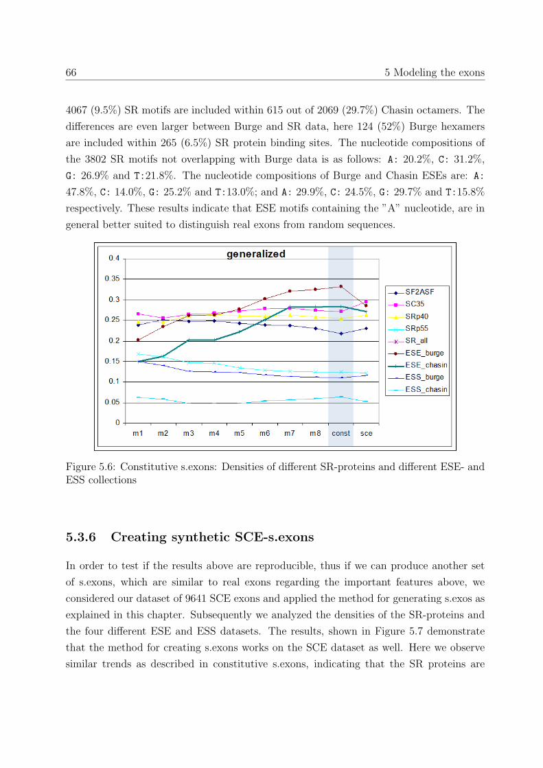
66 5 Modeling the exons
4067 (9.5%) SR motifs are included within 615 out of 2069 (29.7%) Chasin octamers. The
differences are even larger between Burge and SR data, here 124 (52%) Burge hexamers
are included within 265 (6.5%) SR protein binding sites. The nucleotide compositions of
the 3802 SR motifs not overlapping with Burge data is as follows: A: 20.2%, C: 31.2%,
G: 26.9% and T:21.8%. The nucleotide compositions of Burge and Chasin ESEs are: A:
47.8%, C: 14.0%, G: 25.2% and T:13.0%; and A: 29.9%, C: 24.5%, G: 29.7% and T:15.8%
respectively. These results indicate that ESE motifs containing the ”A” nucleotide, are in
general better suited to distinguish real exons from random sequences.
Figure 5.6: Constitutive s.exons: Densities of different SR-proteins and different ESE- andESS collections
5.3.6 Creating synthetic SCE-s.exons
In order to test if the results above are reproducible, thus if we can produce another set
of s.exons, which are similar to real exons regarding the important features above, we
considered our dataset of 9641 SCE exons and applied the method for generating s.exos as
explained in this chapter. Subsequently we analyzed the densities of the SR-proteins and
the four different ESE and ESS datasets. The results, shown in Figure 5.7 demonstrate
that the method for creating s.exons works on the SCE dataset as well. Here we observe
similar trends as described in constitutive s.exons, indicating that the SR proteins are
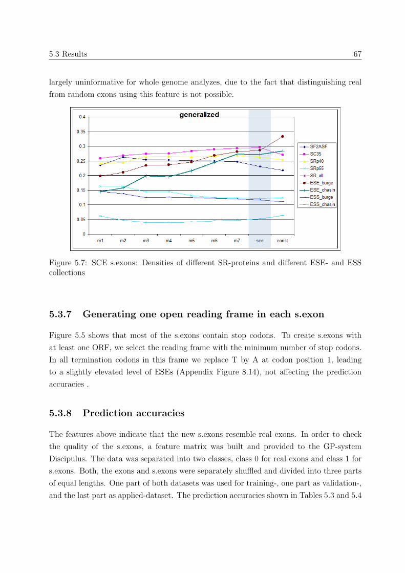
5.3 Results 67
largely uninformative for whole genome analyzes, due to the fact that distinguishing real
from random exons using this feature is not possible.
Figure 5.7: SCE s.exons: Densities of different SR-proteins and different ESE- and ESScollections
5.3.7 Generating one open reading frame in each s.exon
Figure 5.5 shows that most of the s.exons contain stop codons. To create s.exons with
at least one ORF, we select the reading frame with the minimum number of stop codons.
In all termination codons in this frame we replace T by A at codon position 1, leading
to a slightly elevated level of ESEs (Appendix Figure 8.14), not affecting the prediction
accuracies .
5.3.8 Prediction accuracies
The features above indicate that the new s.exons resemble real exons. In order to check
the quality of the s.exons, a feature matrix was built and provided to the GP-system
Discipulus. The data was separated into two classes, class 0 for real exons and class 1 for
s.exons. Both, the exons and s.exons were separately shuffled and divided into three parts
of equal lengths. One part of both datasets was used for training-, one part as validation-,
and the last part as applied-dataset. The prediction accuracies shown in Tables 5.3 and 5.4

68 5 Modeling the exons
are achieved on the data unknown to the GP-system, the applied dataset. Table 5.3 shows
the results on the generalized approach; Table 5.4 shows the specific approach results. For
both approaches, the prediction accuracies drop down as the quality of the model increases.
The more accurate a model of the real data seemed to be; the more difficult it was for the
GP-system to distinguish s.exons from exons. Starting with the very primitive model m1,
81.1% of the data was classified correctly by guessing the s.exons right in 82.6% of all cases
(sensitivity), and predicting real exons 79.6% accurately (specificity). However, random
data looks real and vice versa in almost 19% of all cases. As we considered the exact
same length distributions we can conclude that random data can also have properties of
real exons regarding the features considered. The best models generated with the general
approach were still easily predictable by the GP-system, with an accuracy of almost 70%
(Table 5.3). Thereby the sensitivity was always higher compared to the specificity. The
reason for this observation is explained in the ”best features” section.
A better approximation of real data could be reached with the specific approach (Table
5.4). The prediction accuracies dropped down quickly for the first three models, wordlength
1 - 3, from 75.7% to 62.9%, and it continued to drop down slowly until a plateau of 57-58%
could be reached for wordlength 6-10. These results indicate that a further increase of
the wordlength will not necessarily lead to better results. To ensure that the result of 7%
above a prediction accuracy for tossing a coin (=50%) in wordlength 10 s.exons is caused
by real features rather than by some GP- artifacts, the outputs on training, validation and
applied datasets were shuffled. By shuffling the outputs, features of the two classes are
randomly assigned to either class 0 or class 1, leading into a coin tossing scenario with
an expected prediction accuracy of 50%. The control dataset fits the expectation (Table
5.4). The features responsible for the 7% higher prediction accuracies are shown in next
chapter, Figure 5.9.
It is interesting to note that the prediction accuracy on reverse- vs. real exons was 96.7%.
This implies that the exonic sequence is not only carrying the information for protein
synthesis (in case of protein coding exons), but also every exon carries the information
of a reading direction, which is encoded in simple dinucleotides. A similar result was
also reached on a dataset of 2046 human pseudo exons, whereas in A.thaliana only 90.6%
accuracy was reached. The reasons for this observation are still unclear.

5.3 Results 69
Table 5.3: Prediction accuracies with the generalized approach
model sensitivity specificity (sen+spe)/2m1 82.55 79.64 81.09m2 80.11 74.06 77.08m3 80.07 72.72 76.40m4 83.55 69.80 76.68m5 77.00 67.62 72.31
adjusted m5 82.46 63.19 72.83m6 79.37 61.87 70.62m7 82.06 57.15 69.61m8 79.09 59.95 69.52
Table 5.4: Prediction accuracies with the specific approach
model sensitivity specificity (sen+spe)/2reverse exons 96.73 96.73 96.73wordlength 1 78.5 72.89 75.70wordlength 2 69.17 68.18 68.68wordlength 3 61.35 64.37 62.86wordlength 4 56.33 64.31 60.32wordlength 5 68.81 49.38 59.10wordlength 6 60.95 55.83 58.39wordlength 7 58.37 57.24 57.81wordlength 8 53.92 62.26 58.09wordlength 9 57.85 57.06 57.46wordlength 10 53.18 62.35 57.77
control set(wordlength 10
with shuffled output) 54.09 46.52 50.31
5.3.9 Best features
For each experiment the used features within the best 30 programs (out of several millions
of programs) have been collected and analyzed. The best features used for the discrimi-
nation between real exons and the generalized s.exons; respectively real exons and specific
approach s.exons are shown in Figures 5.8 and 5.9. The best features on the generalized
approach data are nucleotides frequencies. The most often used feature is frequency of

70 5 Modeling the exons
nucleotide Cytosine, followed by nucleotide frequency of Adenine, Thymine and Guanine.
Also the features ”enhancers” and ”tgga” are used for discrimination. The more complex
models, like m6, m7 and m8 do not rely on the features ”enhancer” and ”tgga” but almost
solely on a,c,g and t.

5.3 Results 71
Figure 5.8: Feature frequencies on generalized approach data.

72 5 Modeling the exons
Figure 5.9: Feature frequencies on specific approach data.

5.3 Results 73
This observation indicates that the former features have been modeled more accurately
within the s.exons than the nucleotide frequencies, which needed to be further investigated.
The distributions of the a, c, g, t densities within the generalized model m7 and the
constitutive dataset are shown in Figure 5.10. Although dealing with almost similar number
of e.g. the letter ”a” in constitutive exons (there are 1132915 ”a”s in the dataset of all
27519 exons) and m7 s.exons (1129736 ”a”s), the distributions are not similar. Real exons
have a higher frequency of cases where single nucleotides seem to be depleted or enriched
compared to s.exons, which shapes the distributions in general broader for each of the four
nucleotides. The greatest differences between real and s.exon data can be observed within
Cytosine and Adenine. A possible reason for this observation could be that building blocks
for exons carrying a low number of a certain nucleotide, tend to cluster with ones with
the same properties. A further observation is shown in Appendix Figures 8.7 and 8.8: the
ratio between different nucleotides. The ratio between Adenine and Cytosine turned out
to be significantly different between s.exons and exons (Result of TTest: 3.3E-236).
Figure 5.10: Distribution of the A, C, G, T nucleotide fractions in generalized data m7versus const

74 5 Modeling the exons
5.4 Conclusions
Starting with the construction of generalized synthetic exons, we did not find a ”general
formula” to explain how real exons are built. Although we were able to find a rule to
successfully reconstruct the correct ESE and ESS densities (models m7 and m8 in Figures
5.2 and 5.4), the nucleotide composition in s.exons is more homogenous in comparison with
real exons (Figure 5.10). The differences between the frequencies of single nucleotides are
more pronounced in real exons, especially regarding the ratios of A to C (Figure 8.7). The
GP-system uses this information - the ratios between the four different nucleotides - as the
most important features (particularly in the more complex models m6-m8)(Figure 5.8), to
achieve high prediction accuracies of 70%. The reason for the heterogenous character of
real exons is yet still unclear, a possible explanation could be that special circumstances
might require special types of exons, with more pronounced nucleotide differences in order
to facilitate/prevent binding of specific factors. In this context, it would be interesting to
investigate, whether exons with different splice patterns in different tissues or developmen-
tal stages, might as well have different nucleotide compositions.
Creating a second class of synthetic exons, the specific approach s.exons, solves the prob-
lem of homogenous nucleotide distributions and drops prediction accuracies down, until
a plateau of 57-58% is reached for wordlengths 6-10, indicating that a further increase of
the wordlengths will not necessarily lead to better results (Figure 5.4). Shuffling the exon
pieces of different wordlengths, results however, in an ESE density below the original data
(average ESE density in wordlength 10: 27.5% vs. 29.8% in constitutive exons)(Figure
5.3), and is thus not well suited to generate sequences with exonic properties regarding
the feature ESE densities. Unfortunately, it is not possible to combine the advantages of
both, the specific and the generalized method, e.g. by calculating the triplet transition
probability matrix for every exon (instead for all exons), as this approach would lead in
most cases either to identical exons (in some cases also to truncated exons); due to the
incompleteness of the probability matrix, caused by the short nature ( 150 bp length) of
exons.
In addition to the ESEs densities, we were also able to reconstruct the ESE-networks, of the
most frequently co-occurring words (m7 in Figure 5.2), indicating that our triplet transition
probability approach, implemented in m7 and m8 s.exons is well suited to capture sequence
properties.
We find that the ”A”-feature plays an important role in ESE networks, as it is significantly

5.4 Conclusions 75
enriched in motifs co-occurring together. Another finding is that the densities of the SR
proteins binding sites, cannot be used as a feature to distinguish real from random ex-
ons, however these motifs are generally depleted in adenines, thus these results indicate
that ESE motifs containing the ”A” nucleotide, are in general better suited to distinguish
real exons from random sequences. A biological explanation for the repeated GAA mo-
tifs detected in ESE-networks of constitutive and m7 s.exons, can be explained by the
Tra2 proteins, which are known to be ESE and which preferentially, bind to GAA-repeats
(Tacke, Tohyama, Ogawa, and Manley 1998).
Our results indicate that the generalized synthetic exons are a promising, however improv-
able approach to capture sequence properties of real exons. A possible improvement of the
generalized s.exons can be realized by destroying the sequence homogeneity detected in m7
s.exons by enriching the amounts of ”A”s or ”C”s proportional to the original distribution
but dependent upon which of the two nucleotides is in excess.

Chapter 6
Alternative splicing and evolution
6.1 Introduction
Comparisons of human and mouse transcript sequences have revealed that the vast ma-
jority (more than 80%) of alternative splicing events have not been conserved during
the ∼80- to 90-million-year interval, separating these species (Modrek and Lee 2003;
Yeo et al. 2005; Nurtdinov et al. 2003; Pan et al. 2005). These results indicate that
purifying selection is not acting on such a large time scale to preserve the same patterns
of alternative splicing. Species-specific alternative splicing events have been predicted to
modify conserved domains in proteins and thus to provide an additional potential source
of complexity and differences between mammals (Pan et al. 2005). More recent studies
consider a smaller timescale of a ∼6-million-year interval, between the human and chim-
panzee split. Despite an overall sequence identity between human and chimpanzee genomic
coding regions of 98%-99%, the authors have reported that 6%-8% of profiled orthologous
exons display pronounced splicing level differences in the corresponding tissues from the
two species (Calarco et al. 2007).
In the first part of this chapter, we consider an even smaller time-scale, the intra-species
timescale within humans, spanning 100,000 years of divergence between the Asian, African
and European populations. We apply two population genetical test statistics, which mea-
sure deviations from the standard neutral model to investigate whether selection, positive
or negative, acts differently in alternatively than in constitutively spliced exons.
In the second part of this chapter, we investigate the origins of intron retention. Here, we
expansion the time-scale from the intra-species population genetical age (∼ 100kyears) to

6.2 Analyzing skipped exons with population genetical measures of selection 77
the inter-species timescale (∼80- to 90-million-years) by comparing orthologous regions of
human retained introns, with chimp, mouse, rat, cow and zebrafish.
6.2 Analyzing skipped exons with population geneti-
cal measures of selection
6.2.1 Background
Despite the increasing importance of alternative splicing in various fields such as oncology,
developmental biology, and molecular medicine, its role in the context of evolution has not
been explored in detail.
In a key study by Modrek and Lee (Modrek and Lee 2003), it is suggested that alterna-
tive splicing may be used as a playground for evolution incorporating new exons into only a
few transcripts of a gene (”minor-form” transcripts) and at the same time maintaining the
gene’s functionality by the ”major-form” transcripts. Minor-form exons may be free from
functional constraints and negative selection. In this way alternative splicing would allow
an organism to convert low-fitness forms faster to higher fitness forms, after a series of mu-
tations resulting in a new, useful function (Boue et al. 2003). Evidence for relaxation of
selection pressure during the evolution includes e.g. the observation that AS is associated
with an accelerated rate of exon creation and loss (Modrek and Lee 2003), that new exon
originations from Alu-elements are alternatively spliced (Sorek et al. 2002), and that al-
ternatively spliced isoforms have a much higher frequency of premature termination codons
(PTCs) (Xing and Lee 2004; Lewis et al. 2003; Grellscheid and Smith 2006).
Recent studies have focussed on comparative genomics by using orthologous exons in
different genomes - mostly from human and mouse - to explore the rates of synonymous
(nucleotide substitutions not changing the protein) and non-synonymous (substitutions
changing the protein) divergence (Xing and Lee 2006; Plass and Eyras 2006;
Xing and Lee 2005; Ermakova et al. 2006; Cusack and Wolfe 2005;
Chen et al. 2006). The so-called ”Ka/Ks ratio test” (also known as dN/dS ratio test) is
based on the assumption that most genes are subject to purifying selection with stronger
selective constraints for non-synonymous substitutions (Nekrutenko et al. 2002).
Non-synonymous substitutions occur less frequently (Ka<Ks) and the ratio Ka/Ks
has been found to be significantly smaller than 1 for most protein coding regions

78 6 Alternative splicing and evolution
(Makalowski and Boguski 1998). Applying of this method to alternatively and
constitutively spliced exons revealed that conserved alternative exons have higher Ka rates
than average, indicating a relaxation of evolutionary constraints (Xing and Lee 2005;
Ermakova et al. 2006; Chen et al. 2006). However these studies are mainly based on
comparisons of protein coding regions between different species. In this study we focus
on within species analyses of coding and non-coding exons in humans and find that
Tajima’s D is smaller in the skipped compared to the constitutive exon dataset. We
also find a slightly elevated level of genetic diversity in a distance of 1-7 bp next to the
splice boundaries in alternative exons, but at the same time a decreased average number
of SNPs in the flanking regions, supporting the recent finding of increased purifying
selection in exon flanks (Xing et al. 2006). However, the results above are affected by an
ascertainment bias in human genome-wide polymorphism data, and turn out not to be
significant after the correction of the ascertainment bias by using a method proposed by
Nielsen et al.(Clark et al. 2005).
6.2.2 Materials and Methods
The SNP data are from the release 21 of the Hapmap Project, available in September 2006
(Thorisson et al. 2005). The samples we refer to in the following as ”African”, ”Euro-
pean” and ”Asian” are from 90 individuals (30 parent-offspring trios) from the Yoruba in
Ibadan, Nigeria (abbreviation YRI); 90 individuals (30 trios) in Utah, USA, from the Cen-
tre d’Etude du Polymorphisme Humain collection (abbreviation CEU); 45 Han Chinese
in Beijing, China (abbreviation CHB); 44 Japanese in Tokyo, Japan (abbreviation JPT)
(Frazer et al. 2007; Barnes 2006).
Tajima’s test of neutral mutation hypothesis
Tajima’s test is based on the relationship between the number of segregating sites (S) and
the average pairwise diversity (Π)(Tajima 1989). Both quantities depend on mutation rate
(µ) and effective population size (Ne), which can hardly be estimated separately empiri-
cally. The composite parameter θ = 4Neµ can be estimated from both, S and Π. Let the
estimates of θ be θS and θΠ, respectively. The expectation of these estimates is identi-
cal under neutrality (θS = θΠ). The normalization of their difference D= θΠ−θS√V ar(θΠ−θS)
is
called Tajima’s D and can be used as a statistic to test the hypothesis of neutral evolution.
Directional selection leads to an excess of rare variants, therefore a disproportionally in-
creased value of θS and, as a consequence, a negative D. D>0 suggest an excess of common

6.2 Analyzing skipped exons with population genetical measures of selection 79
variation, which is consistent with balancing selection or population contraction. D>0 can
also be due to ascertainment bias, i.e. artefactual absence of rare variants.
Linkage Disequilibrium (LD)
Linkage disequilibrium is the non-random association of two alleles from two loci (e.g. A
and B) on the same chromosome. LD measures the difference between the observed allele
frequencies for a two locus allele (PAB) as compared to its expected frequency, which is
the product of the two single allele frequencies (PA*PB). In case LD is around zero, alleles
at the two loci tend to be inherited in a nearly random manner.
6.2.3 Results and Discussion
Tajima’s D and LD Analysis
The average Tajima’s D values for the constitutive and alternative regions of the Hapmap
populations are shown in Table 6.1. It may be surprising that the Tajima’s D values
are contrary to the neutral theory in average not around 0, but consistently higher. The
reason for this observation is not balancing selection but the fact that a great portion of
rare SNP data is simply missing in the Hapmap database because of ascertainment bias.
An extensive analysis and debate on the ascertainment bias in studies of human genome-
wide polymorphism can be found in (Clark et al. 2005). By comparing the alternative
with the constitutive dataset we observe a significant decrease in the Tajima’s D values
within all populations, indicating either traces of population growth or traces of directional
selection in regions with alternative splicing (Table 6.1).
A section of regions with negative Tajima’s D values demonstrates that not only the curve
of the derived population (red) is shifted to the more negative values compared to the
ancestral population (black), but also the curve of the alternative regions is shifted to the
more negative side, encouraging the findings above (Figure 6.1).
SNP density and distribution
Various recent studies have reported that regions flanking a skipped exon are generally
more conserved (Modrek and Lee 2003; Sorek and Ast 2003; Kaufmann et al. 2004;
Philipps et al. 2004), whereas the splice sites themselves are weaker [39]. By analyzing
SNPs from Hapmap we observe a slightly elevated level of genetic diversity very close to

80 6 Alternative splicing and evolution
Table 6.1: Tajima’s D and LD results on the dataset of the regions with constitutivelyspliced and skipped exons
constitutive skipped p-value t-testTajima’s D
Africa (YRI) 0.552 0.426 <0.01Asia (CHB+JPT) 0.219 0.113 0.001
Europe (CEU) 0.351 0.213 <0.01LD
Africa (YRI) 0.799 0.812 0.077Asia (CHB+JPT) 0.859 0.870 0.101
Europe (CEU) 0.845 0.859 0.062
Figure 6.1: negative Tajima’s D for alternative and constitutive regions in Europe andAfrica
the splice boundaries in alternative exons compared to constitutive exons and at the same
time a decreased average number of SNPs with increasing distance (Fig. 6.2).
It is interesting to note that the upstream regions of a skipped exon bear a smaller number
of SNPs compared to the constitutive exons but also compared to the downstream regions.
This observation might be explained by the fact that alternative exons are in general

6.2 Analyzing skipped exons with population genetical measures of selection 81
Figure 6.2: SNPs in intronic regions flanking the exons
more tightly regulated than constitutive and the upstream regions contain more conserved
sequence motifs e.g.: motifs for the branch point recognition and miscellaneous exonic
splicing enhancer and silencer.
Figure 6.3: Hapmap: SNP density in protein coding regions
The average SNP density per base pair in protein coding regions is shown in Fig. 6.3
Almost no differences between the constitutive and the SCE data are observable in the
up- and downstream exons; whereas the variability decreases in SCE exons and in their

82 6 Alternative splicing and evolution
flanking introns, compared to the constitutive dataset.
SNPdb: synonymous and non-synonymous SNPs within protein coding exons
The picture above (Figure 6.3) changes when considering the entire dataset of 10mio
SNPs from dbSNP, build 124 (Sherry et al. 2001). The alternative variants, as well as
their flanking exons show here a higher degree of variability, whereas the flanking introns
display less differences (Fig. 6.4). We also downloaded the information about the type of
the SNP, weather it is a synonymous or an amino acid changing non-synonymous SNP.
The result is shown in Fig. 6.5. In general constitutive, as well as their flanking exons
have a smaller number of synonymous SNPs per base pair, compared to exon skipping
events (Fig. 6.5.a.). This effect even increases when taking into account non-synonymous
SNPs. In case of constitutive regions, the SNP rate of non-synonymous SNPs decreases
(compared to synonymous SNPs), whereas it is elevated in skipped exons and exons that
flank them (Fig. 6.5.b.). One explanation for this observation could be that in case of
constitutive exons we see purifying selection acting on the sequences in order to prevent,
a possibly disrupting, amino acid change. The alternative counterpart seems to be under
less evolutionary constraints as it is not included in every transcript. It is important to
note that the other reason for the contrasting results Genome wide evolutionary analyses
has therefore to consider that SNPs from SNPdb do not have a controlled sample size
while HapMap contains only a subset of all human SNPs. As Fig. 6.4 shows these two
aspects lead to quite contrasting results, for instance, of the amount of polymorphisms in
alternatively and constitutively spliced genes.
Species-specific splicing
Pan et al. showed that alternative splicing of conserved exons is frequently species-specific
in human and mouse (Pan et al. 2005). They have estimated that >11% of conserved hu-
man and mouse cassette exons undergo skipping in one species but constitutively splicing
in the other. These species-specific alternative splicing events are predicted to modify con-
served domains in proteins and thus constitute an additional potential source of complexity
and species-specific differences between mammals (Pan et al. 2005). We have downloaded
the data from their supplementary material, which contains three classes of exons. In addi-
tion to species-specific spliced exons, there are also conserved and gene specific alternative
events. Conserved exons are detected as alternative in both species, whereas gene-specific
exons can only be found in one of the two species. By reanalyzing their data we observe

6.2 Analyzing skipped exons with population genetical measures of selection 83
Figure 6.4: SNPdb: SNP density in protein coding regions
Figure 6.5: SNP types in protein coding regions: a. synonymous SNPs, b. non-synonymousSNPs
that Tajima’s D values seem to be smaller on species-specific spliced genes. Although the
t-test reveals that this difference is not significant in Europe and Africa (Table 6.2), in Asia
we observe a significant access of directional selection acting upon species-specific spliced
genes.

84 6 Alternative splicing and evolution
Table 6.2: Calculating Tajima’s D on Pan et al. data
Conserved Gene Specific Species Specific p-value t-testAsia
Ø Tajima’s D 0.351 0.086 -0.014 0.001Std. Deviation 1.129 1.219 1.172
EuropeØ Tajima’s D 0.294 0.266 0.159 0.214Std. Deviation 1.123 1.198 1.188
AfricaØ Tajima’s D 0.381 0.401 0.318 0.535Std. Deviation 1.045 1.082 1.053
Adjusting for the ascertainment bias
The HapMap SNP database has been designed to support disease association studies by
determining the common patterns of DNA sequence variation in the human genome, in
DNA samples from populations with ancestry from Africa, Asia and Europe. However,
it was not primarily designed for population genetical purposes. The main focus of the
project was on common alleles instead of rare alleles; therefore the rare ones tend to be
missing. To test at which extent the lack of rare alleles affects the results, we analyzed
the ENCODE regions from HapMap, which contain an approximate tenfold higher density
of SNPs (NN 2005). Unfortunately, none of our exons were included in these regions.
We compared the percentage of monomorphic SNPs in ENCODE vs. other HapMap re-
gions and found that in ENCODE regions there is in average an increase of 13% of this
type of rare alleles in all three populations. In the case of the well analyzed FOXP2 gene
[9], HapMap reports only 9 SNPs instead of the experimentally validated 47 SNPs. The
Tajima’s D values are higher for the HapMap SNPs, by taking into consideration all pop-
ulations; HapMap yields a Tajima’s D value of -1 vs. -2.2. In order to correct for the
ascertainment bias we used the method developed by Nielsen et al. (Clark et al. 2005),
which predicts the properties of missing SNPs, based on a Maximum Likelihood (ML)
method. By using this method on the HapMap data, we approximate the real value above
and achieve after correction a Tajima’s value of -1.79. This method was also applied to
the data in Table 6.1 resulting in a loss of the signal, due to similar results for conserved
and specific exons (Tajima’s D: -1.20).

6.3 On the origins of intron retention 85
6.2.4 Conclusions
Initially, we found that Tajima’s D was significantly smaller in the skipped compared to
the constitutive exon dataset in all three populations, indicating an elevated level of di-
rectional selection in alternatively spliced genes. Linkage Disequilibrium was higher in
derived populations and in alternatively spliced genes in all populations. We also found a
slightly elevated level of genetic diversity next to the splice boundaries in alternative ex-
ons but at the same time a decreased average number of single nucleotide polymorphisms
(SNPs), providing evidence for increased purifying selection. However, after correction
of the ascertainment bias, the differences within constitutively and alternatively spliced
genes, detected with Tajima’s D in the experiments above, disappeared completely. In-
stead showing significant differences, the Tajima’s D values were undistinguishable similar
between constitutive and alternative genes in all populations, as well as in the case of
species-specific splicing. Additional problems were the incomplete SNP databases, leading
to contradicting results. Based on these results, we conclude that the evolutionary role of
alternative splicing remains, at least for the moment speculative.
6.3 On the origins of intron retention
6.3.1 Background
Since the discovery in 1978 that eukaryotes have in contrast to prokaryotes, a split
gene structure containing exons and introns (Gilbert 1978), there have been heated de-
bates about the origins of spliceosomal introns, which continues today. The two main
schools of thought are the introns-early and the introns-late theories. According to the
introns-early theory, introns were already present in the progenote, the common ances-
tor of eukaryotes and prokaryotes, and were lost in the course of evolution in prokary-
otes by selection towards compact genomes and short generation times (Gilbert 1978;
Artamonova and Gelfand 2007; Doolittle 1978). This theory is based on the obser-
vations that in many cases exons coincide with protein domains, either functional or struc-
tural, which may represent early, primitive genes. A central prediction of this theory is that
the early introns were mediators that facilitated the early assembly of proteins by accelerat-
ing the rate of exon-shuffling (Palmer and Logsdon 1991). The introns-late-theory pro-
poses an insertion of introns into eukaryotic genomes after the split with prokaryotes. Thus,

86 6 Alternative splicing and evolution
exon-shuffling played no role in the assembly of early genes (Palmer and Logsdon 1991).
This theory is supported by numerous examples of recent intron gain and also by the fact
that some unicellular eukaryotes have no or very few introns. However, recent studies
that are based on large-scale genome comparisons reveal that the extremes of both theo-
ries are mistaken, as there clearly exists both ancient exons and recently inserted introns
(Artamonova and Gelfand 2007). We are interested in characterizing the evolutionary
role of intron retention in human, where an intron can either be spliced out or stay retained
in the mature mRNA, and e.g. thereby change the protein product. It has been reported
that 17% of all alternative splicing variants are of this type in humans (Stamm et al. 2006).
In order to investigate whether the retained introns are in most cases introns that are
changing their properties to become new exons, we analyzed 1468 human SIR introns from
the AltSplice database and compared them with orthologous regions in other species. We
found that most cases of intron retention in human are not conserved beyond the primate
lineage. Our data suggest that this observation is not solely the result of lower EST and
cDNA coverage in other species, but it is rather a consistent trend of exon gain in pri-
mates, supporting the introns-early theory. However, we also find that EST data are a
strong limiting factor and that the entries in EST databases are not always reliable (e.g.
wrong labeled Chimp data), therefore the data is in general to sparse to allow derivation
of rules, yet.
6.3.2 Results
Splicing in orthologous regions of other species
In order to have a reliable and more up-to-date dataset, we filtered 1468 cases where the
introns were flanked by an up- and downstream-exon as annotated in Ensembl (04/2007).
We started with 1468 cases of ”SIR” and searched for orthologous regions in chimp, mouse,
rat, cow and zebrafish, by using the LiftOver tool from the UCSC webpage (Kent 2002).
1028 cases were discarded from further analysis, as they were not conserved in all species
(however, only 238 cases were discarded, when not considering the zebrafish). We calcu-
lated the Intron Retention Levels in all species based on current EST and cDNA data,
downloaded from the UCSC webpage (Kent 2002). It is important to note, that although
the EST data downloaded from UCSC was labeled as ”Chimp”, we found out that it did
not originate solely from ”Chimp”, but rather from ”Human” instead. The reasons for the
mis-labeling are yet unclear, thus they affect our results, as ”primate specific” findings,

6.3 On the origins of intron retention 87
might only be ”human specific”.
Further 32 cases, where at least one species was not covered by EST/cDNA at all, were
discarded as well. The most prevalent picture of the data was alternative splicing in human
and chimp but constitutive in all other species (198 out of a total of 408 conserved cases),
indicating an excess of this type of splicing in the ”primate lineage”. In order to depict this
finding we calculated a ”splicing parsimony tree” for the species, based on the alignments
of the alternative splicing events (Fig. 6.6). Thereby, for each of the 408 conserved intronic
regions, we assigned a ”1” in case of a SIR event and a ”0” in case of constitutive splicing,
for each species. E.g., ”110000” was the most frequently observed pattern (198/408 cases),
indicating SIR splicing in human and chimp, and constitutive splicing in mouse, rat, cow
and zebrafish. The resulting ”splicing parsimony tree”, shown in Fig. 6.6, does not depict
the correct evolutionary distances; however it indicates rather an excess of SIR type of
splicing in the ”primate lineage”. Another explanation for the big distance between the
”primates” and the other species, might as well be the different EST/cDNA coverage levels
within the different species. To eliminate the factor ”EST-coverage”, the following section
compares only ESTs with a ”good” coverage in other species.
Figure 6.6: Analysed intron retention events are restricted to primate specific lineages
ESTs with ”good” coverage in other species
In order to test if the elevated level of intron retention events in human and chimp may
be caused only by a better EST coverage in these two species, we analyzed the proportion
of ”comparable EST coverage”, defined as follows: the other species should bear no more
than 10% less ESTs/or more ESTs relative to human. Results are shown in Table 6.3.
”New” events are defined as follows: intron retention is observable in human but not in
the other compared species. ”Loss” is the opposite case. An increase of retained intron
events in human could be detected, although the EST coverage was on average larger for

88 6 Alternative splicing and evolution
Table 6.3: Events with comparable EST coverage between human and another species
AverageESTs in
cases withCases with comparablecomparable EST no IR in
EST coverage coverage ”New” ”Loss” both IR in bothHS vs. Chimp 1312 247 vs. 252 31 5 267 1009
in % 2.4% 0.4% 20.4% 76.9%HS vs. Mouse 243 75 vs. 95 139 7 42 55
in % 57.2% 2.9% 17.3% 22.6%HS vs. Rat 11 15 vs. 69 8 0 3 1
in % 66.7% 0% 25.0% 8.3%HS vs. Cow 65 24 vs. 41 42 2 14 7
in % 64.6% 3.1% 21.5% 10.8%HS vs. Zebrafish 13 30 vs. 82 10 0 3 0
in % 76.9% 0% 23.1% 0%
the other species (Tab. 6.3). However, the number of comparable cases (e.g. 243 in mouse,
and 11 in rat) is too small, to derive general conclusions that intron retention is new in
humans.
22 most recent SIR events
When analyzing the acceptor splice sites, greater splice site strength and also a pattern of
consecutive T-s can be observed in constitutive introns. The interesting point in Figure 6.7
is the pattern at the 3’ splice site of the 22 human specific retained introns, which appears
to be more divergent from the consensus.
In order to investigate the reason for the disrupted motif above (Fig. 6.7), we aligned the
last 14 intronic nucleotides, upstream of a 3’splice site in human to the mouse genome and
observed that in 25 of 61 mutations a Thymine in mouse (Tm) is exchanged by a Cytosine
in human (Ch), resulting in a weaker 3’ splice site strength. Out of all possible mutation
varieties, the ChTm pattern is observed in more than 40% of all cases (Appendix Figure
8.16).
Extending the view to more general cases, with ”good” EST coverage in mouse
To ensure that the findings above are not solely based on the very low number of human

6.3 On the origins of intron retention 89
Figure 6.7: Sequence logos for donor- and acceptor splice sites
specific cases (22 introns), we extended the dataset. A number of 139 intron retention
events in human were constitutive in mouse and had ”good” EST coverage. We also
included chimp for comparison. The analysis of these events reveals a T→C exchange in
the primate lineage (Appendix Figure 8.17).
Comparison between human constitutive introns and mouse alternative introns
To take care that the T→C exchange between human and mouse is not based upon different
GC-contents between the two species, we performed the following inverse test: we compared
297 constitutive human introns with ”good” EST coverage against alternatively spliced,
(retained introns) orthologous introns in mouse and found the opposite of the previously
obtained pattern, indicating that a lack of T might be connected to an alternative way of
intron splicing (Appendix Figure 8.18).
Estimating the evolutionary age of retained introns
Similar in spirit to the idea by Zhang and Chasin (Zhang and Chasin 2006), of separating
exons according to their evolutionary ages, here we compared the dataset of short ConstI
(introduced in Chapter 3.5) with the SIR dataset. Short constIs were thereby well suited
for this task, as they have the similar length distributions as SIR and are therefore not
too long to be not conserved in different species. We investigated whether their orthologs
could be found in the chimpanzee, dog, mouse, rat, chicken, zebrafish, and fugu genomes.
We reasoned that a human intron whose ortholog is present in a given organism must
have been ”born” before the divergence between humans and that organism. In case the
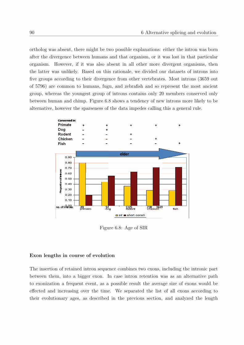
90 6 Alternative splicing and evolution
ortholog was absent, there might be two possible explanations: either the intron was born
after the divergence between humans and that organism, or it was lost in that particular
organism. However, if it was also absent in all other more divergent organisms, then
the latter was unlikely. Based on this rationale, we divided our datasets of introns into
five groups according to their divergence from other vertebrates. Most introns (3659 out
of 5796) are common to humans, fugu, and zebrafish and so represent the most ancient
group, whereas the youngest group of introns contains only 20 members conserved only
between human and chimp. Figure 6.8 shows a tendency of new introns more likely to be
alternative, however the sparseness of the data impedes calling this a general rule.
Figure 6.8: Age of SIR
Exon lengths in course of evolution
The insertion of retained intron sequence combines two exons, including the intronic part
between them, into a bigger exon. In case intron retention was as an alternative path
to exonization a frequent event, as a possible result the average size of exons would be
effected and increasing over the time. We separated the list of all exons according to
their evolutionary ages, as described in the previous section, and analyzed the length
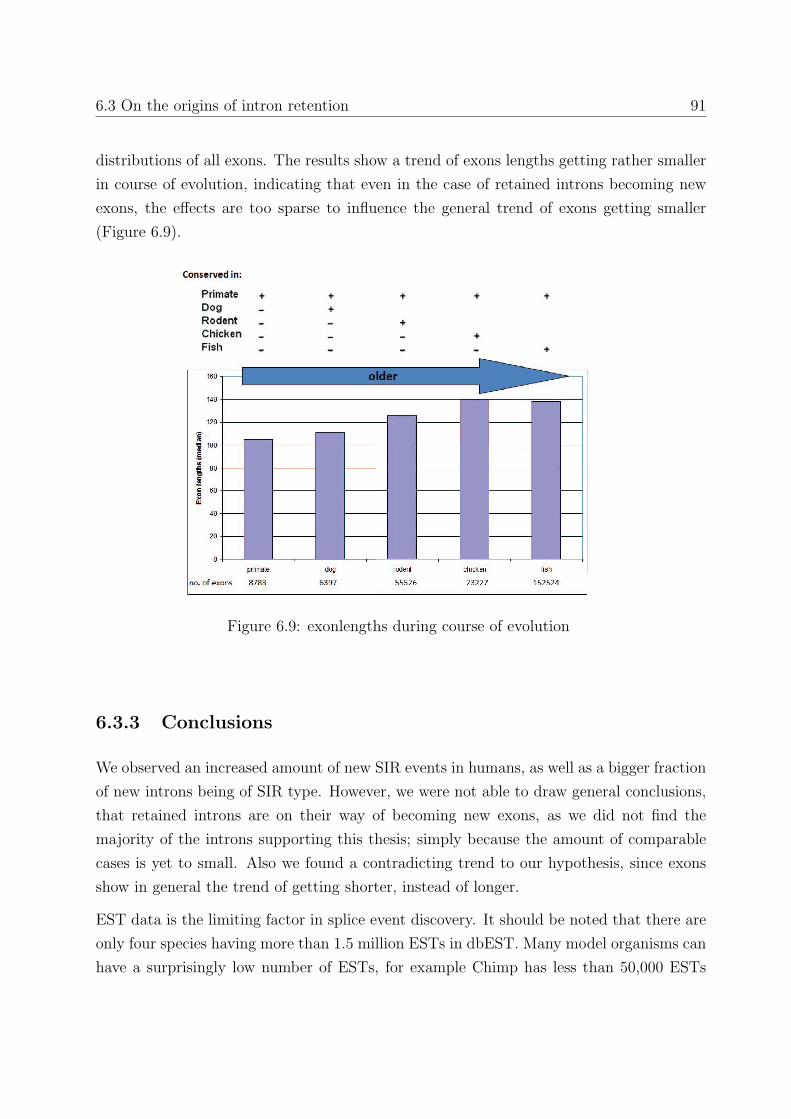
6.3 On the origins of intron retention 91
distributions of all exons. The results show a trend of exons lengths getting rather smaller
in course of evolution, indicating that even in the case of retained introns becoming new
exons, the effects are too sparse to influence the general trend of exons getting smaller
(Figure 6.9).
Figure 6.9: exonlengths during course of evolution
6.3.3 Conclusions
We observed an increased amount of new SIR events in humans, as well as a bigger fraction
of new introns being of SIR type. However, we were not able to draw general conclusions,
that retained introns are on their way of becoming new exons, as we did not find the
majority of the introns supporting this thesis; simply because the amount of comparable
cases is yet to small. Also we found a contradicting trend to our hypothesis, since exons
show in general the trend of getting shorter, instead of longer.
EST data is the limiting factor in splice event discovery. It should be noted that there are
only four species having more than 1.5 million ESTs in dbEST. Many model organisms can
have a surprisingly low number of ESTs, for example Chimp has less than 50,000 ESTs

92 6 Alternative splicing and evolution
(September 2008). Thus, it is likely that many splice events in these organisms remain to
be detected.
We would like to emphasize that data analysis can only be as good as the raw data are.
Wrong inferences are foreseeable, if data are wrongly annotated as for instance ”Chimp
ESTs” which in fact are derived from human.
Chapter 7
Summary and Outlook
The motivation behind this project was to decipher how the splicing information is encoded
within the human genomic sequence, and how this information is used to specify whether
an exon or intron has the potential to be spliced alternatively or not. The concept thereby
was not to rely on data inaccessible to the organism, such as sequence conservation levels
to other species, but to only use the intrinsic sequence information of the human genome.
By using the GP-System Discipulus, we attempted to simulate the decision process (al-
ternative or not) of the spliceosome, by collecting important splicing signals/information,
and condensing them (in form of a feature matrix) into the GP-System. Discipulus is
designed to detect the most important features for binary classification problems, and to
combine them with one another in order to find the best partition rules. We started with a
very simple model for alternative splicing prediction, containing only nucleotide informa-
tion within exons, and later extended the feature matrix by including information present
within up- and downstream exons and introns. We analyzed 27,519 constitutively spliced
and 9,641 cassette exons (SCE) together with their neighboring introns; in addition we
analyzed 33,316 constitutively spliced introns and 2,712 retained introns (SIR). We find
that our tool for classifying yields highly accurate predictions on the SIR data, with a
sensitivity of 92.1% and a specificity of 79.2%. Prediction accuracies on the SCE data are
lower: 47.3% (sensitivity) and 70.9% (specificity), indicating that alternative splicing of
introns can be better captured by sequence properties than that of exons.
The most frequently used feature for classification of SIRs was the silencer score, which can
be explained by our discovery that retained introns appeared to harbor ”exon properties”
and were clearly distinguishable from constitutive introns, regarding this feature cf. (Figure
3.3).

94 7 Summary and Outlook
To address the low prediction accuracy of correctly classifying SCEs, we incorporated
information in addition to canonical splicing signals (such as information about the splice
site strength, the branch point, the polypyrimidine tract and secondary structure features).
In the interest of thoroughness, we tested various other approaches such as: A-stretches,
ESE composition, ESE transformation, etc., as well as evolutionary features (Chapter 6);
we even reversed the sequences and investigated the reversed sequence (data not shown).
However, despite all of the above approaches taken, none could increase the prediction
accuracy of correctly classifying SCEs to a level of more than 60%. In the case of SCE, the
GP-System preferred the A-feature over any other feature, which at the time, was an unan-
swered question. Further investigation revealed that ”feature A” is especially enriched in
the most abundant exonic splicing enhancers, found in constitutive exons (Chapter 3.4.2),
as well as in ESE networks of constitutive exons (Chapter 5.3.2). Moreover, we detected
a certain repetitive motif, GAA in constitutive exons that was absent from SCEs in the
most abundant exonic splicing enhancers and ESE networks. These GAA repeats are char-
acteristic of many enhancer elements, e.g., they are known binding sites for Tra2 proteins
(Tacke, Tohyama, Ogawa, and Manley 1998). However, when looking at individual exons,
the signal is also found in many SCE exons and therefore it is impossible to predict the
alternative splicing variant.
Training solely with the ”A”-feature, the prediction accuracy already reached a prediction
level of 58.2%, which is only ∼1% below the GP run containing the complete feature
matrix with 35 features. Excluding this feature caused a drop in the prediction accuracy
of ∼1%. We found that, in order to achieve the same results as with 35 features, it is
sufficient to use only the five features with the highest impact values (Figure 3.4): A, C,
GGG, and the splice sites. This result also implies that the features themselves are not
connected to each other, e.g. counter-intuitively, in constitutive exons, weak splice sites
are not compensated by a higher level of ESEs (at least this pattern was not seen on a
large scale in this analysis).
As seen in Figure 3.4 there is no optimal combination of features that can be used by the
GP-system to solve the alternative splicing classification problem, in contrast to classifi-
cation of reverse exons (Figure 8.6),where a combination of features resulted in prediction
accuracies of > 96%.
It should be mentioned that with our original feature matrix (of 35 features) and the
GP-System we used, we could solve the easier task of classifying exons versus introns,
7 Summary and Outlook 95
with a high fidelity rate of 95.58% (sens.: 96.05, spec.: 95.10). This result supports our
hypothesis that the DNA sequence, although containing the information on its orientation
and whether a part of it is exonic or intronic, does not contain the complete information
required for alternative splicing. Based on our finding for SCE, we suggest that only 20%
(on scala between 50%(coin-toss) and 100%(always correct), we reach a prediction accuracy
of 60%) of the entire information for alternative splicing is encoded at the sequence level.
In the case of retained introns, we could show that by comparing SIRs with short constI
decreased the initial accuracy of ∼85% to a level of only ∼64%, suggesting that in this
case, 30% of the alternative splicing information is harbored in the sequence. To ensure
that the findings above are not the result of an outdated or untrustworthy dataset of exons
and introns, in Chapter 3.4.6., we separated the datasets based upon their inclusion levels,
into seven different partitions. We investigated each of the seven partition using a large
amount of various ESE and ESS signals, without observing any difference between any of
the inclusion level classes. This similarity between the classes lends even further support
to our hypothesis that there is insufficient information encoded solely within the RNA
sequence to dictate alternative splicing. In addition to sequence, the presence or absence
of proteins (possibly tissue specific, developmental stage specific, etc.,) actually recognizing
and binding theses sequences constitutes the other half of the information content.
Clearly, there are many improvements that can be made in order to increase the efficacy of
alternative splice form classification and prediction. One such improvement lies within the
precise delineation of core splicing motifs e.g. only a few dozen branch point sites have been
reliably defined of mammalian sequences. As of yet, a reliable sequence model to predict
such branch point sites is still lacking(Wang and Burge 2008). Furthermore, although we
are aware of ESE densities, we can not be certain that there is a direct correlation of
increased densities and increased splicing trans-factor binding.
Taken together all of our results imply that alternative splicing might be largely governed
by trans-acting processes which currently pose a great experimental and computational
challenge. Furthermore the question remains if there is a general rule that can encapsulate
the phenomenon of alternative splicing or if one must appeal to laborious gene-by-gene
approach to understand its underlying mechanism. In other words, can we compile a
universal splicing code that interweaves the actions of cis and trans acting elements, along
with the rules that operate during specific developmental stages or in particular cell types.
Developing such a code, if possible, is a distinct challenge for the future.
In the last chapter we investigated the question whether alternative splicing may be con-

96 7 Summary and Outlook
nected to adaptive evolutionary processes in a species or population. Unfortunately, the
currently available population genetical tools were not sensitive enough to identify traces of
positive or balancing selection on the scale of a few 100bp. Moreover, the current amount
of EST data is another limiting factor in splice event discovery, as currently there are only
four species having more than 1.5 million ESTs in dbEST. Additional problems are the in-
complete SNP databases and SNP ascertainment bias. The evolutionary role of alternative
splicing remains, at least for the moment, speculative. Taking into account the growing
amounts of data available in future, we are optimistic that it will be interesting to repeat
the experiments introduced in Chapter 6 in only a few years.

References
Alberts, B., D. Bray, and J. Lewis, 2002 M olecular biology of the cell (4th editioned.). Taylor and Francis.
Artamonova, I. and M. Gelfand, 2007, Aug)Comparative genomics and evolution ofalternative splicing: the pessimists’ science. Chem. Rev. 107: 3407–3430.
Ast, G., 2004, Oct)How did alternative splicing evolve? Nat. Rev. Genet. 5: 773–782.
Baek, D. and P. Green, 2005, Sep)Sequence conservation, relative isoform frequencies,and nonsense-mediated decay in evolutionarily conserved alternative splicing. Proc.Natl. Acad. Sci. U.S.A. 102: 12813–12818.
Banzhaf, W., P. Nordin, R. Keller, and F. Francone, 1998 Genetic Program-ming: An Introduction - On the Automatic Evolution of Computer Programs and ItsApplications. Heidelberg: dpunkt.
Barnes, M., 2006, Sep)Navigating the HapMap. Brief. Bioinformatics 7: 211–224.
Behm-Ansmant, I., I. Kashima, J. Rehwinkel, J. Sauliere, N. Wittkopp, andE. Izaurralde, 2007, Jun)mRNA quality control: an ancient machinery recognizesand degrades mRNAs with nonsense codons. FEBS Lett. 581: 2845–2853.
Berget, S., 1995, Feb)Exon recognition in vertebrate splicing. J. Biol. Chem. 270: 2411–2414.
Birney, E., D. Andrews, M. Caccamo, Y. Chen, L. Clarke, G. Coates, T. Cox,F. Cunningham, V. Curwen, T. Cutts, T. Down, R. Durbin, X. Fernandez-Suarez, P. Flicek, S. Graf, M. Hammond, J. Herrero, K. Howe, V. Iyer,K. Jekosch, A. Kahari, A. Kasprzyk, D. Keefe, F. Kokocinski, E. Kule-sha, D. London, I. Longden, C. Melsopp, P. Meidl, B. Overduin, A. Parker,G. Proctor, A. Prlic, M. Rae, D. Rios, S. Redmond, M. Schuster, I. Sealy,S. Searle, J. Severin, G. Slater, D. Smedley, J. Smith, A. Stabenau,J. Stalker, S. Trevanion, A. Ureta-Vidal, J. Vogel, S. White, C. Wood-wark, and T. Hubbard, 2006, Jan)Ensembl 2006. Nucleic Acids Res. 34: D556–561.

98 REFERENCES
Black, D., 2003 Mechanisms of alternative pre-messenger RNA splicing. Annu. Rev.Biochem. 72: 291–336.
Blencowe, B., 2000, Mar)Exonic splicing enhancers: mechanism of action, diversity androle in human genetic diseases. Trends Biochem. Sci. 25: 106–110.
Boguski, M., 1995, Aug)The turning point in genome research. Trends Biochem. Sci. 20:295–296.
Boue, S., I. Letunic, and P. Bork, 2003, Nov)Alternative splicing and evolution.Bioessays 25: 1031–1034.
Brett, D., J. Hanke, G. Lehmann, S. Haase, S. Delbruck, S. Krueger, J. Re-ich, and P. Bork, 2000, May)EST comparison indicates 38mRNAs contain possiblealternative splice forms. FEBS Lett. 474: 83–86.
Brown, T. A., 1999 M oderne Genetik. Heidelberg - Berlin: Spektrum AkademischerVerlag.
Brudno, M., M. Gelfand, S. Spengler, M. Zorn, I. Dubchak, and J. Conboy,2001a, Jun)Computational analysis of candidate intron regulatory elements for tissue-specific alternative pre-mRNA splicing. Nucleic Acids Res. 29: 2338–2348.
Brudno, M., M. Gelfand, S. Spengler, M. Zorn, I. Dubchak, and J. Conboy,2001b, Jun)Computational analysis of candidate intron regulatory elements for tissue-specific alternative pre-mRNA splicing. Nucleic Acids Res. 29: 2338–2348.
Burge, C., T. Tuschl, and P. Sharp. Splicing of precursors to mRNAs by the spliceo-somes. The RNA world.
Calarco, J., Y. Xing, M. Caceres, J. Calarco, X. Xiao, Q. Pan, C. Lee,T. Preuss, and B. Blencowe, 2007, Nov)Global analysis of alternative splicingdifferences between humans and chimpanzees. Genes Dev. 21: 2963–2975.
Cartegni, L., S. Chew, and A. Krainer, 2002, Apr)Listening to silence and under-standing nonsense: exonic mutations that affect splicing. Nat. Rev. Genet. 3: 285–298.
Cartegni, L., J. Wang, Z. Zhu, M. Zhang, and A. Krainer, 2003, Jul)ESEfinder: Aweb resource to identify exonic splicing enhancers. Nucleic Acids Res. 31: 3568–3571.
Cartegni, L., J. Wang, Z. Zhu, M. Q. Zhang, and A. R. Krainer, 2008, Au-gust)ESEfinder. http://rulai.cshl.edu/tools/ESE2/ESEmatrix.html.
Caceres, J. and A. Kornblihtt, 2002, Apr)Alternative splicing: multiple control mech-anisms and involvement in human disease. Trends Genet. 18: 186–193.
Chen, F., S. Wang, C. Chen, W. Li, and T. Chuang, 2006, Mar)Alternativelyand constitutively spliced exons are subject to different evolutionary forces. Mol. Biol.Evol. 23: 675–682.
Chern, T., E. van Nimwegen, C. Kai, J. Kawai, P. Carninci, Y. Hayashizaki, andM. Zavolan, 2006, Apr)A simple physical model predicts small exon length variations.PLoS Genet. 2: e45.

REFERENCES 99
Clark, A., M. Hubisz, C. Bustamante, S. Williamson, and R. Nielsen, 2005,Nov)Ascertainment bias in studies of human genome-wide polymorphism. GenomeRes. 15: 1496–1502.
Clark, F. and T. Thanaraj, 2002, Feb)Categorization and characterization oftranscript-confirmed constitutively and alternatively spliced introns and exons fromhuman. Hum. Mol. Genet. 11: 451–464.
Cohen, M. and B. Emanuel, 1994, Dec)Expressed sequence tags. Science 266: 1790–1791.
Conrads, M., W. Banzhaf, P. Nordin, R. Keller, and F. Francone, 2001 Dis-cipulus - Fast Genetic Programming Based on AIM Learning Technology.
Consortium, I., 2004, Oct)Finishing the euchromatic sequence of the human genome.Nature 431: 931–945.
Cristianini, N. and J. Shawe-Taylor, 2004 K ernel Methods for Pattern Analysis.Cambridge, MA,: Cambridge University Press.
Cusack, B. and K. Wolfe, 2005, Nov)Changes in alternative splicing of human andmouse genes are accompanied by faster evolution of constitutive exons. Mol. Biol.Evol. 22: 2198–2208.
Dahmcke, C. and C. Mitchelmore, 2008 Altered splicing in exon 8 of the DNA repli-cation factor CIZ1 affects subnuclear distribution and is associated with Alzheimer’sdisease. Mol. Cell. Neurosci. 38: 589–594.
Doolittle, W. F., 1978 Genes in pieces: were they ever together? Nature 272: 581–582.
Dror, G., R. Sorek, and R. Shamir, 2005, Apr)Accurate identification of alternativelyspliced exons using support vector machine. Bioinformatics 21: 897–901.
Ermakova, E., R. Nurtdinov, and M. Gelfand, 2006 Fast rate of evolution inalternatively spliced coding regions of mammalian genes. BMC Genomics 7: 84.
Eyras, E., M. Caccamo, V. Curwen, and M. Clamp, 2004, May)ESTGenes: alter-native splicing from ESTs in Ensembl. Genome Res. 14: 976–987.
Fairbrother, W. G., R.-F. Yeh, P. A. Sharp, and C. B. Burge, 2002 Predictiveidentification of exonic splicing enhancers in human genes. Science 297: 1007–1013.
Florea, L., G. Hartzell, Z. Zhang, G. Rubin, and W. Miller, 1998, Sep)A com-puter program for aligning a cDNA sequence with a genomic DNA sequence. GenomeRes. 8: 967–974.
Francone, F. D., M. Conrads, W. Banzhaf, and P. Nordin, 1999, 13-17July)Homologous Crossover in Genetic Programming. In W. Banzhaf, J. Daida, A. E.Eiben, M. H. Garzon, V. Honavar, M. Jakiela, and R. E. Smith (Eds.), Proceedings ofthe Genetic and Evolutionary Computation Conference, Volume 2, Orlando, Florida,USA, pp. 1021–1026. Morgan Kaufmann.

100 REFERENCES
Frank D. Francone, Markus Conrads, W. B. and P. Nordin, 1999, 13-17July)Homologous Crossover in Genetic Programming. In A. E. E. M. H. G. V. H.M. J. Wolfgang Banzhaf, Jason Daida and R. E. Smith (Eds.), Proceedings of the Ge-netic and Evolutionary Computation Conference, Volume 2, Orlando, Florida, USA,pp. 1021–1026. Morgan Kaufmann.
Frazer, K., D. Ballinger, D. Cox, D. Hinds, L. Stuve, R. Gibbs, J. Bel-mont, A. Boudreau, P. Hardenbol, S. Leal, S. Pasternak, D. Wheeler,T. Willis, F. Yu, H. Yang, C. Zeng, Y. Gao, H. Hu, W. Hu, C. Li,W. Lin, S. Liu, H. Pan, X. Tang, J. Wang, W. Wang, J. Yu, B. Zhang,Q. Zhang, H. Zhao, H. Zhao, J. Zhou, S. Gabriel, R. Barry, B. Blu-menstiel, A. Camargo, M. Defelice, M. Faggart, M. Goyette, S. Gupta,J. Moore, H. Nguyen, R. Onofrio, M. Parkin, J. Roy, E. Stahl, E. Winch-ester, L. Ziaugra, D. Altshuler, Y. Shen, Z. Yao, W. Huang, X. Chu, Y. He,L. Jin, Y. Liu, Y. Shen, W. Sun, H. Wang, Y. Wang, Y. Wang, X. Xiong,L. Xu, M. Waye, S. Tsui, H. Xue, J. Wong, L. Galver, J. Fan, K. Gun-derson, S. Murray, A. Oliphant, M. Chee, A. Montpetit, F. Chagnon,V. Ferretti, M. Leboeuf, J. Olivier, M. Phillips, S. Roumy, C. Sallee,A. Verner, T. Hudson, P. Kwok, D. Cai, D. Koboldt, R. Miller, L. Paw-likowska, P. Taillon-Miller, M. Xiao, L. Tsui, W. Mak, Y. Song, P. Tam,Y. Nakamura, T. Kawaguchi, T. Kitamoto, T. Morizono, A. Nagashima,Y. Ohnishi, A. Sekine, T. Tanaka, T. Tsunoda, P. Deloukas, C. Bird,M. Delgado, E. Dermitzakis, R. Gwilliam, S. Hunt, J. Morrison, D. Pow-ell, B. Stranger, P. Whittaker, D. Bentley, M. Daly, P. de Bakker,J. Barrett, Y. Chretien, J. Maller, S. McCarroll, N. Patterson, I. Pe’er,A. Price, S. Purcell, D. Richter, P. Sabeti, R. Saxena, S. Schaffner,P. Sham, P. Varilly, D. Altshuler, L. Stein, L. Krishnan, A. Smith,M. Tello-Ruiz, G. Thorisson, A. Chakravarti, P. Chen, D. Cutler,C. Kashuk, S. Lin, G. Abecasis, W. Guan, Y. Li, H. Munro, Z. Qin,D. Thomas, G. McVean, A. Auton, L. Bottolo, N. Cardin, S. Eyher-amendy, C. Freeman, J. Marchini, S. Myers, C. Spencer, M. Stephens,P. Donnelly, L. Cardon, G. Clarke, D. Evans, A. Morris, B. Weir,T. Tsunoda, J. Mullikin, S. Sherry, M. Feolo, A. Skol, H. Zhang, C. Zeng,H. Zhao, I. Matsuda, Y. Fukushima, D. Macer, E. Suda, C. Rotimi, C. Ade-bamowo, I. Ajayi, T. Aniagwu, P. Marshall, C. Nkwodimmah, C. Royal,M. Leppert, M. Dixon, A. Peiffer, R. Qiu, A. Kent, K. Kato, N. Ni-ikawa, I. Adewole, B. Knoppers, M. Foster, E. Clayton, J. Watkin,R. Gibbs, J. Belmont, D. Muzny, L. Nazareth, E. Sodergren, G. Wein-stock, D. Wheeler, I. Yakub, S. Gabriel, R. Onofrio, D. Richter, L. Ziau-gra, B. Birren, M. Daly, D. Altshuler, R. Wilson, L. Fulton, J. Rogers,J. Burton, N. Carter, C. Clee, M. Griffiths, M. Jones, K. McLay,R. Plumb, M. Ross, S. Sims, D. Willey, Z. Chen, H. Han, L. Kang, M. God-bout, J. Wallenburg, P. L’Archeveque, G. Bellemare, K. Saeki, H. Wang,
REFERENCES 101
D. An, H. Fu, Q. Li, Z. Wang, R. Wang, A. Holden, L. Brooks, J. McEwen,M. Guyer, V. Wang, J. Peterson, M. Shi, J. Spiegel, L. Sung, L. Zacharia,F. Collins, K. Kennedy, R. Jamieson, and J. Stewart, 2007, Oct)A secondgeneration human haplotype map of over 3.1 million SNPs. Nature 449: 851–861.
Gao, K., A. Masuda, T. Matsuura, and K. Ohno, 2008, Apr)Human branch pointconsensus sequence is yUnAy. Nucleic Acids Res. 36: 2257–2267.
Gilbert, W., 1978, Feb)Why genes in pieces? Nature 271: 501.
Gooding, C., F. Clark, M. Wollerton, S. Grellscheid, H. Groom, andC. Smith, 2006 A class of human exons with predicted distant branch points revealedby analysis of AG dinucleotide exclusion zones. Genome Biol. 7: R1.
Goren, A., O. Ram, M. Amit, H. Keren, G. Lev-Maor, I. Vig, T. Pupko,and G. Ast, 2006, Jun)Comparative analysis identifies exonic splicing regulatorysequences–The complex definition of enhancers and silencers. Mol. Cell 22: 769–781.
Graveley, B., 2000 Sorting out the complexity of SR protein functions. RNA 6: 1197–1211.
Green, R., B. Lewis, R. Hillman, M. Blanchette, L. Lareau, A. Garnett,D. Rio, and S. Brenner, 2003 Widespread predicted nonsense-mediated mRNAdecay of alternatively-spliced transcripts of human normal and disease genes. Bioinfor-matics 19 Suppl 1: i118–121.
Grellscheid, S. and C. Smith, 2006, Mar)An apparent pseudo-exon acts both as analternative exon that leads to nonsense-mediated decay and as a zero-length exon. Mol.Cell. Biol. 26: 2237–2246.
Hiller, M., K. Huse, M. Platzer, and R. Backofen, 2005 Non-EST based predictionof exon skipping and intron retention events using Pfam information. Nucleic AcidsRes. 33: 5611–5621.
Hiller, M., K. Huse, K. Szafranski, N. Jahn, J. Hampe, S. Schreiber, R. Back-ofen, and M. Platzer, 2004, Dec)Widespread occurrence of alternative splicing atNAGNAG acceptors contributes to proteome plasticity. Nat. Genet. 36: 1255–1257.
Hiller, M., K. Szafranski, R. Backofen, and M. Platzer, 2006, Nov)Alternativesplicing at NAGNAG acceptors: simply noise or noise and more? PLoS Genet. 2: e207;author reply e208.
Hofacker, I. and P. Stadler, 2006, May)Memory efficient folding algorithms for cir-cular RNA secondary structures. Bioinformatics 22: 1172–1176.
Holste, D. and U. Ohler. T.
Holste, D. and U. Ohler, 2008, Jan)Strategies for identifying RNA splicing regulatorymotifs and predicting alternative splicing events. PLoS Comput. Biol. 4: e21.
Jiang, H., R. Teng, Q. Wang, X. Zhang, H. Wang, Z. Wang, J. Cao, and L. Teng,2008 Transcriptional analysis of estrogen receptor alpha variant mRNAs in colorectalcancers and their matched normal colorectal tissues. J. Steroid Biochem. Mol. Biol.

102 REFERENCES
Johnson, J., J. Castle, P. Garrett-Engele, Z. Kan, P. Loerch, C. Armour,R. Santos, E. Schadt, R. Stoughton, and D. Shoemaker, 2003, Dec)Genome-wide survey of human alternative pre-mRNA splicing with exon junction microarrays.Science 302: 2141–2144.
Jumaa, H. and P. Nielsen, 1997, Aug)The splicing factor SRp20 modifies splicing of itsown mRNA and ASF/SF2 antagonizes this regulation. EMBO J. 16: 5077–5085.
Jurica, M., 2008, Jun)Detailed close-ups and the big picture of spliceosomes. Curr. Opin.Struct. Biol. 18: 315–320.
Jurica, M. and M. Moore, 2003, Jul)Pre-mRNA splicing: awash in a sea of proteins.Mol. Cell 12: 5–14.
Kalnina, Z., P. Zayakin, K. Silina, and A. Lin, 2005, Apr)Alterations of pre-mRNAsplicing in cancer. Genes Chromosomes Cancer 42: 342–357.
Kaufmann, D., O. Kenner, P. Nurnberg, W. Vogel, and B. Bartelt, 2004,Feb)In NF1, CFTR, PER3, CARS and SYT7, alternatively included exons show higherconservation of surrounding intron sequences than constitutive exons. Eur. J. Hum.Genet. 12: 139–149.
Kent, W., 2002, Apr)BLAT–the BLAST-like alignment tool. Genome Res. 12: 656–664.
Kerenyi, Z., Z. Merai, L. Hiripi, A. Benkovics, P. Gyula, C. Lacomme,E. Barta, F. Nagy, and D. Silhavy, 2008, Jun)Inter-kingdom conservation of mech-anism of nonsense-mediated mRNA decay. EMBO J. 27: 1585–1595.
Kim, E., A. Goren, and G. Ast, 2008a Alternative splicing and disease. RNA Biol 5:17–19.
Kim, E., A. Goren, and G. Ast, 2008b, Jan)Alternative splicing: current perspectives.Bioessays 30: 38–47.
Kol, G., G. Lev-Maor, and G. Ast, 2005, Jun)Human-mouse comparative analysis re-veals that branch-site plasticity contributes to splicing regulation. Hum. Mol. Genet. 14:1559–1568.
Koza, J., 1992 Genetic Programming: On the Programming of Computers by Means ofNatural Selection. Cambridge:The MIT Press.
Lander and all, 2001, Feb)Initial sequencing and analysis of the human genome. Na-ture 409: 860–921.
Lejeune, F. and L. Maquat, 2005, Jun)Mechanistic links between nonsense-mediatedmRNA decay and pre-mRNA splicing in mammalian cells. Curr. Opin. Cell Biol. 17:309–315.
Lewis, B., R. Green, and S. Brenner, 2003, Jan)Evidence for the widespread couplingof alternative splicing and nonsense-mediated mRNA decay in humans. Proc. Natl.Acad. Sci. U.S.A. 100: 189–192.

REFERENCES 103
Lim, L. and C. Burge, 2001, Sep)A computational analysis of sequence features involvedin recognition of short introns. Proc. Natl. Acad. Sci. U.S.A. 98: 11193–11198.
Lim, L. and P. Sharp, 1998, Jul)Alternative splicing of the fibronectin EIIIB exon de-pends on specific TGCATG repeats. Mol. Cell. Biol. 18: 3900–3906.
Liu, H., M. Zhang, and A. Krainer, 1998, Jul)Identification of functional exonic splic-ing enhancer motifs recognized by individual SR proteins. Genes Dev. 12: 1998–2012.
Makalowski, W. and M. Boguski, 1998, Aug)Synonymous and nonsynonymous sub-stitution distances are correlated in mouse and rat genes. J. Mol. Evol. 47: 119–121.
Maniatis, T. and R. Reed, 2002, Apr)An extensive network of coupling among geneexpression machines. Nature 416: 499–506.
Markowetz, F., 2008, August)Klassifikation mit SVM. http://lectures.molgen.mpg.de/statistik03/docs/Kapitel 16.pdf.
Matlin, A., F. Clark, and C. Smith, 2005, May)Understanding alternative splicing:towards a cellular code. Nat. Rev. Mol. Cell Biol. 6: 386–398.
McCullough, A. and S. Berget, 1997, Aug)G triplets located throughout a class ofsmall vertebrate introns enforce intron borders and regulate splice site selection. Mol.Cell. Biol. 17: 4562–4571.
McGuire, A., M. Pearson, D. Neafsey, and J. Galagan, 2008 Cross-kingdompatterns of alternative splicing and splice recognition. Genome Biol. 9: R50.
McKeown, M., 1992 Alternative mRNA Splicing. Annual Reviews Cellular Biology 8:133–155.
Minovitsky, S., S. Gee, S. Schokrpur, I. Dubchak, and J. Conboy, 2005 Thesplicing regulatory element, UGCAUG, is phylogenetically and spatially conserved inintrons that flank tissue-specific alternative exons. Nucleic Acids Res. 33: 714–724.
Miriami, E., H. Margalit, and R. Sperling, 2003, Apr)Conserved sequence elementsassociated with exon skipping. Nucleic Acids Res. 31: 1974–1983.
Mironov, A., J. Fickett, and M. Gelfand, 1999, Dec)Frequent alternative splicingof human genes. Genome Res. 9: 1288–1293.
Mitchell, T., 1997 M achine Learning. McGraw-Hill.
Modrek, B. and C. Lee, 2002, Jan)A genomic view of alternative splicing. Nat.Genet. 30: 13–19.
Modrek, B. and C. Lee, 2003, Jun)Alternative splicing in the human, mouse and ratgenomes is associated with an increased frequency of exon creation and/or loss. Nat.Genet. 34: 177–180.
Nagaraj, S., R. Gasser, and S. Ranganathan, 2007, Jan)A hitchhiker’s guide toexpressed sequence tag (EST) analysis. Brief. Bioinformatics 8: 6–21.

104 REFERENCES
NC-IUB, 2004, Februar)Nomenclature for Incompletely Specified Bases in Nucleic AcidSequences. http://www.chem.qmul.ac.uk/iubmb/misc/naseq.html.
Needleman, S. and C. Wunsch, 1970, Mar)A general method applicable to the searchfor similarities in the amino acid sequence of two proteins. J. Mol. Biol. 48: 443–453.
Nekrutenko, A., K. Makova, and W. Li, 2002, Jan)The K(A)/K(S) ratio test forassessing the protein-coding potential of genomic regions: an empirical and simulationstudy. Genome Res. 12: 198–202.
Nilsen, T., 2003, Dec)The spliceosome: the most complex macromolecular machine inthe cell? Bioessays 25: 1147–1149.
Nilsson, N., 1996 Introduction to Machine Learning.
NN. dbEST.
NN. info on dbEST from 2006-2007.
NN. Info on GenBank.
NN. Info on GenBank.
NN, 2005, Oct)A haplotype map of the human genome. Nature 437: 1299–1320.
NN, 2008a, August)info on dbEST from 2005. http://drnelson.utmem.edu/msci814.module1.html.
NN, 2008b, August)UCSC - Genome Browser. ftp://hgdownload.cse.ucsc.edu/goldenPath/hg18/.
Nurtdinov, R., I. Artamonova, A. Mironov, and M. Gelfand, 2003, Jun)Lowconservation of alternative splicing patterns in the human and mouse genomes. Hum.Mol. Genet. 12: 1313–1320.
Ohler, U., N. Shomron, and C. Burge, 2005, Jul)Recognition of unknown conservedalternatively spliced exons. PLoS Comput. Biol. 1: 113–122.
Pagani, F. and F. Baralle, 2004, May)Genomic variants in exons and introns: identi-fying the splicing spoilers. Nat. Rev. Genet. 5: 389–396.
Palmer, J. and J. Logsdon, 1991, Dec)The recent origins of introns. Curr. Opin. Genet.Dev. 1: 470–477.
Pan, Q., M. Bakowski, Q. Morris, W. Zhang, B. Frey, T. Hughes, andB. Blencowe, 2005, Feb)Alternative splicing of conserved exons is frequently species-specific in human and mouse. Trends Genet. 21: 73–77.
Pan, Q., A. Saltzman, Y. Kim, C. Misquitta, O. Shai, L. Maquat, B. Frey, andB. Blencowe, 2006, Jan)Quantitative microarray profiling provides evidence againstwidespread coupling of alternative splicing with nonsense-mediated mRNA decay tocontrol gene expression. Genes Dev. 20: 153–158.
Philipps, D., J. Park, and B. Graveley, 2004, Dec)A computational and experimentalapproach toward a priori identification of alternatively spliced exons. RNA 10: 1838–1844.

REFERENCES 105
Plass, M. and E. Eyras, 2006 Differentiated evolutionary rates in alternative exonsand the implications for splicing regulation. BMC Evol. Biol. 6: 50.
Pozzoli, U. and M. Sironi, 2005, Jul)Silencers regulate both constitutive and alternativesplicing events in mammals. Cell. Mol. Life Sci. 62: 1579–1604.
Raetsch, G., S. J. Schultheiss, and C. S. Ong, 2008 Free Support Vector Machine.http://galaxy.fml.tuebingen.mpg.de/.
Reed, R. and T. Maniatis, 1985, May)Intron sequences involved in lariat formationduring pre-mRNA splicing. Cell 41: 95–105.
Romfo, C., C. Alvarez, W. van Heeckeren, C. Webb, and J. Wise, 2000,Nov)Evidence for splice site pairing via intron definition in Schizosaccharomyces pombe.Mol. Cell. Biol. 20: 7955–7970.
Roy, S. and W. Gilbert, 2006, Mar)The evolution of spliceosomal introns: patterns,puzzles and progress. Nat. Rev. Genet. 7: 211–221.
Ratsch, G., S. Sonnenburg, and B. Scholkopf, 2005, Jun)RASE: recognition ofalternatively spliced exons in C.elegans. Bioinformatics 21 Suppl 1: i369–377.
Rudd, S., 2003, Jul)Expressed sequence tags: alternative or complement to whole genomesequences? Trends Plant Sci. 8: 321–329.
Sakabe, N. and S. de Souza, 2007 Sequence features responsible for intron retentionin human. BMC Genomics 8: 59.
Scholkopf, B. and A. Smola, 2002 Learning with Kernels: Support Vector Machines,Regularization, Optimization, and Beyond (Adaptive Computation and Machine Learn-ing). Cambridge, MA,: MIT Press.
Senapathy, P., M. Shapiro, and N. Harris, 1990 Splice junctions, branch point sites,and exons: sequence statistics, identification, and applications to genome project. Meth.Enzymol. 183: 252–278.
Sharma, S., L. Kohlstaedt, A. Damianov, D. Rio, and D. Black, 2008,Feb)Polypyrimidine tract binding protein controls the transition from exon definitionto an intron defined spliceosome. Nat. Struct. Mol. Biol. 15: 183–191.
Sherry, S., M. Ward, M. Kholodov, J. Baker, L. Phan, E. Smigielski, andK. Sirotkin, 2001, Jan)dbSNP: the NCBI database of genetic variation. Nucleic AcidsRes. 29: 308–311.
Smith, C. W. J., J. G. Patton, and B. Nadal-Ginard, 1989 Alternative splicing inthe control of gene expression. Annual Reviews Genetic 23: 527–577.
Smith, C. W. J. and J. Valcarcel, 2000 Alternative pre-mRNA splicing: the logic ofcombinatorial control. Trends in Biochemical Sciences 25: 381–388.
Sorek, R. and G. Ast, 2003, Jul)Intronic sequences flanking alternatively spliced exonsare conserved between human and mouse. Genome Res. 13: 1631–1637.

106 REFERENCES
Sorek, R., G. Ast, and D. Graur, 2002, Jul)Alu-containing exons are alternativelyspliced. Genome Res. 12: 1060–1067.
Sorek, R. and H. Safer, 2003, Feb)A novel algorithm for computational identificationof contaminated EST libraries. Nucleic Acids Res. 31: 1067–1074.
Sorek, R., R. Shamir, and G. Ast, 2004, Feb)How prevalent is functional alternativesplicing in the human genome? Trends Genet. 20: 68–71.
Sorek, R., R. Shemesh, Y. Cohen, O. Basechess, G. Ast, and R. Shamir, 2004,Aug)A non-EST-based method for exon-skipping prediction. Genome Res. 14: 1617–1623.
Stamm, S., 2002, Oct)Signals and their transduction pathways regulating alternative splic-ing: a new dimension of the human genome. Hum. Mol. Genet. 11: 2409–2416.
Stamm, S., J. Riethoven, V. Le Texier, C. Gopalakrishnan, V. Kumanduri,Y. Tang, N. Barbosa-Morais, and T. Thanaraj, 2006, Jan)ASD: a bioinformaticsresource on alternative splicing. Nucleic Acids Res. 34: 46–55.
Stoilov, P., R. Daoud, O. Nayler, and S. Stamm, 2004, Mar)Human tra2-beta1autoregulates its protein concentration by influencing alternative splicing of its pre-mRNA. Hum. Mol. Genet. 13: 509–524.
Sugnet, C., W. Kent, M. Ares, and D. Haussler, 2004 Transcriptome and genomeconservation of alternative splicing events in humans and mice. Pac Symp Biocomput:66–77.
Tacke, R., M. Tohyama, S. Ogawa, and J. Manley, 1998, Apr)Human Tra2 proteinsare sequence-specific activators of pre-mRNA splicing. Cell 93: 139–148.
Tajima, F., 1989, Nov)Statistical method for testing the neutral mutation hypothesis byDNA polymorphism. Genetics 123: 585–595.
Talerico, M. and S. Berget, 1990, Dec)Effect of 5’ splice site mutations on splicing ofthe preceding intron. Mol. Cell. Biol. 10: 6299–6305.
Talerico, M. and S. Berget, 1994, May)Intron definition in splicing of small Drosophilaintrons. Mol. Cell. Biol. 14: 3434–3445.
Thanaraj, T., S. Stamm, F. Clark, J. Riethoven, V. Le Texier, and J. Muilu,2004, Jan)ASD: the Alternative Splicing Database. Nucleic Acids Res. 32: D64–69.
Thorisson, G., A. Smith, L. Krishnan, and L. Stein, 2005, Nov)The InternationalHapMap Project Web site. Genome Res. 15: 1592–1593.
Ule, J., G. Stefani, A. Mele, M. Ruggiu, X. Wang, B. Taneri, T. Gaasterland,B. Blencowe, and R. Darnell, 2006, Nov)An RNA map predicting Nova-dependentsplicing regulation. Nature 444: 580–586.
Ule, J., A. Ule, J. Spencer, A. Williams, J. Hu, M. Cline, H. Wang, T. Clark,C. Fraser, M. Ruggiu, B. Zeeberg, D. Kane, J. Weinstein, J. Blume, and

REFERENCES 107
R. Darnell, 2005, Aug)Nova regulates brain-specific splicing to shape the synapse.Nat. Genet. 37: 844–852.
van Nimwegen, E., N. Paul, R. Sheridan, and M. Zavolan, 2006, Apr)SPA: aprobabilistic algorithm for spliced alignment. PLoS Genet. 2: e24.
Venables, J., 2004, Nov)Aberrant and alternative splicing in cancer. Cancer Res. 64:7647–7654.
Voelker, R. and J. Berglund, 2007, Jul)A comprehensive computational characteri-zation of conserved mammalian intronic sequences reveals conserved motifs associatedwith constitutive and alternative splicing. Genome Res. 17: 1023–1033.
Vukusic, I., 2004 Vorhersage von alternativen mRNA Varianten mittels GenetischerProgrammierung. Master’s thesis, Fachbereich Informatik der Universitat Dortmund.
Wang, X., J. Luk, P. Leung, B. Wong, E. Stanbridge, and S. Fan, 2005,Jan)Alternative mRNA splicing of liver intestine-cadherin in hepatocellular carcinoma.Clin. Cancer Res. 11: 483–489.
Wang, Z. and C. Burge, 2008, May)Splicing regulation: from a parts list of regulatoryelements to an integrated splicing code. RNA 14: 802–813.
Wang, Z., M. Rolish, G. Yeo, V. Tung, M. Mawson, and C. Burge, 2004,Dec)Systematic identification and analysis of exonic splicing silencers. Cell 119: 831–845.
Wang, Z., X. Xiao, E. Van Nostrand, and C. Burge, 2006, Jul)General and specificfunctions of exonic splicing silencers in splicing control. Mol. Cell 23: 61–70.
Wheelan, S., D. Church, and J. Ostell, 2001, Nov)Spidey: a tool for mRNA-to-genomic alignments. Genome Res. 11: 1952–1957.
Wirth, B., 2002, Jun)Spinal muscular atrophy: state-of-the-art and therapeutic perspec-tives. Amyotroph. Lateral Scler. Other Motor Neuron Disord. 3: 87–95.
Wollerton, M., C. Gooding, E. Wagner, M. Garcia-Blanco, and C. Smith,2004, Jan)Autoregulation of polypyrimidine tract binding protein by alternative splicingleading to nonsense-mediated decay. Mol. Cell 13: 91–100.
Wu, T. and C. Watanabe, 2005, May)GMAP: a genomic mapping and alignment pro-gram for mRNA and EST sequences. Bioinformatics 21: 1859–1875.
Xing, Y. and C. Lee, 2004, Oct)Negative selection pressure against premature proteintruncation is reduced by alternative splicing and diploidy. Trends Genet. 20: 472–475.
Xing, Y. and C. Lee, 2005, Oct)Assessing the application of Ka/Ks ratio test to alter-natively spliced exons. Bioinformatics 21: 3701–3703.
Xing, Y. and C. Lee, 2006, Jul)Alternative splicing and RNA selection pressure–evolutionary consequences for eukaryotic genomes. Nat. Rev. Genet. 7: 499–509.
Xing, Y., Q. Wang, and C. Lee, 2006, Jul)Evolutionary divergence of exon flanks: adissection of mutability and selection. Genetics 173: 1787–1791.

108 REFERENCES
Yeo, G., S. Hoon, B. Venkatesh, and C. Burge, 2004, Nov)Variation in sequenceand organization of splicing regulatory elements in vertebrate genes. Proc. Natl. Acad.Sci. U.S.A. 101: 15700–15705.
Yeo, G., E. Van Nostrand, D. Holste, T. Poggio, and C. Burge, 2005,Feb)Identification and analysis of alternative splicing events conserved in human andmouse. Proc. Natl. Acad. Sci. U.S.A. 102: 2850–2855.
Yeo, G. W., 2004 Identification, improved modeling and integration of signals to predictconstitutive and altering splicing. Ph. D. thesis, Massachusetts Institute of Technology.Dept. of Brain and Cognitive Sciences.
Zachar, Z., T. Chou, and P. Bingham, 1987, Dec)Evidence that a regulatory geneautoregulates splicing of its transcript. EMBO J. 6: 4105–4111.
Zavolan, M., S. Kondo, C. Schonbach, J. Adachi, D. Hume, Y. Hayashizaki,and T. Gaasterland, 2003, Jun)Impact of alternative initiation, splicing, and termi-nation on the diversity of the mRNA transcripts encoded by the mouse transcriptome.Genome Res. 13: 1290–1300.
Zhang, H., H. Duan, S. Kirley, L. Zukerberg, and C. Wu, 2005, Nov)Aberrantsplicing of cables gene, a CDK regulator, in human cancers. Cancer Biol. Ther. 4:1211–1215.
Zhang, X. and L. Chasin, 2004, Jun)Computational definition of sequence motifs gov-erning constitutive exon splicing. Genes Dev. 18: 1241–1250.
Zhang, X. and L. Chasin, 2006, Sep)Comparison of multiple vertebrate genomes revealsthe birth and evolution of human exons. Proc. Natl. Acad. Sci. U.S.A. 103: 13427–13432.
Zhang, X., K. Heller, I. Hefter, C. Leslie, and L. Chasin, 2003, Dec)Sequenceinformation for the splicing of human pre-mRNA identified by support vector machineclassification. Genome Res. 13: 2637–2650.
Zhang, X., T. Kangsamaksin, M. Chao, J. Banerjee, and L. Chasin, 2005,Aug)Exon inclusion is dependent on predictable exonic splicing enhancers. Mol. Cell.Biol. 25: 7323–7332.
Zheng, C., T. Nair, M. Gribskov, Y. Kwon, H. Li, and X. Fu, 2004 A databasedesigned to computationally aid an experimental approach to alternative splicing. PacSymp Biocomput: 78–88.
Zhou, Z., L. Licklider, S. Gygi, and R. Reed, 2002, Sep)Comprehensive proteomicanalysis of the human spliceosome. Nature 419: 182–185.

Chapter 8
Appendix to chapters 2-6
8.1 Appendix to Chapter 2
The GP-runs are performed with the standard settings of the Discipulus version 3.0.
ADVANCED OPTIONS VALUE
Generations Without Improvement 300Use Adaptive Termination EnabledNumber of depth level 4Width 50Maximum Number of Runs 100Stepping Disabled
FITNESS CALCULATION VALUE
Error Measurement SquarePositive/Negative Threshold 0.5Use Predictor Hit Rate DisabledWeight for Rate of Positive Hits 1Weight for Rate of Negative Hits 1Threshold 1

110 8 Appendix to chapters 2-6
INSTRUCTIONS VALUE
Instruction Set Addition, Arithmetic, Com-parison, Condition (FC-MOVB, FCMOVNB), Datatransfer, Division (all FDIV),Multiplication, Subtraction,Trigonometric
Maximum number of FPU registers 2Ratio Constants / Inputs (%) 50
SEARCH OPERATORS VALUE
Block mutation rate 30Instruction mutation rate 30Instruction data mutation rate 40Homologous crossover 95
PROGRAM SIZE & CONSTANTS VALUE
Initial program size 80Max program size 512Randomize constants amount 53Minimum value -1Maximum value 1
MISCELLANEOUS VALUE
Random Number Generator Seed System timeParsimony Pressure Disabled
GENETIC PROGRAMMING VALUE
Population size 500Mutation frequency % 95Crossover frequency % 50Enable Demes EnabledNumber of demes 10Crossover between demes % 0Migration rate % 1

8.2 Appendix to Chapter 4 111
DYNAMIC SUBSET SELECTION VALUE
Enabled EnabledTarget subset size % 50Selection by age % 50Selection by difficult % 50Stochastic selection % 0Frequency (in generations equivalent) 1
RANDOMIZE VALUE
Randomize Population Size, Maximum Program Size, Num-ber of FPU Registers Used, Subset Size, Percentof Subset Selection by Difficult, Mutation Rate,Crossover Rate, Homologous Crossover Rate, Mi-gration Between Demes Rate
Random Seed System time
Table 8.1: ”Discipulus”-Parameters
8.2 Appendix to Chapter 4
8.2.1 A-stretches
Table 8.2: A-stretches
length A-Stretches SCE SCE-Shuffled (1Run) Const Const-Shuffled(1Run)1 0.7417 0.7365 0.7217 0.72172 0.1811 0.1910 0.1932 0.19773 0.0533 0.0510 0.0579 0.05634 0.0169 0.0148 0.0191 0.01685 0.0054 0.0047 0.0060 0.00526 0.0013 0.0013 0.0017 0.00167 0.0002 0.0004 0.0002 0.00058 0.0000 0.0001 0.0001 0.00029 0.0000 0.0000 0.0000 0.000010 0.0000 0.0000 0.0000 0.0000

112 8 Appendix to chapters 2-6
Table 8.3: distances A-stretches
distance A-Stretches SCE SCE-Shuffled (1Run) Const Const-Shuffled(1Run)d1 0.3200 0.3142 0.3259 0.3214d2 0.1928 0.1853 0.2035 0.1926d3 0.1176 0.1305 0.1185 0.1348d4 0.0894 0.0953 0.0907 0.0957d5 0.0734 0.0693 0.0734 0.0690d6 0.0486 0.0511 0.0461 0.0497d7 0.0369 0.0377 0.0353 0.0360d8 0.0310 0.0282 0.0291 0.0263d9 0.0197 0.0209 0.0182 0.0188d10 0.0152 0.0160 0.0142 0.0140d11 0.0139 0.0123 0.0121 0.0104d12 0.0097 0.0091 0.0074 0.0077d13 0.0068 0.0068 0.0056 0.0056d14 0.0055 0.0053 0.0052 0.0044d15 0.0037 0.0039 0.0031 0.0033d16 0.0032 0.0032 0.0025 0.0024d17 0.0031 0.0024 0.0023 0.0019d18 0.0019 0.0020 0.0014 0.0014d19 0.0015 0.0016 0.0012 0.0011d20 0.0015 0.0012 0.0011 0.0008d21 0.0009 0.0010 0.0007 0.0006d22 0.0008 0.0006 0.0006 0.0006d23 0.0007 0.0006 0.0005 0.0004d24 0.0005 0.0004 0.0003 0.0003d25 0.0004 0.0004 0.0003 0.0002d26 0.0003 0.0003 0.0003 0.0002d27 0.0003 0.0003 0.0002 0.0001d28 0.0003 0.0002 0.0002 0.0001d29 0.0002 0.0002 0.0001 0.0001d30 0.0001 0.0001 0.0001 0.0001
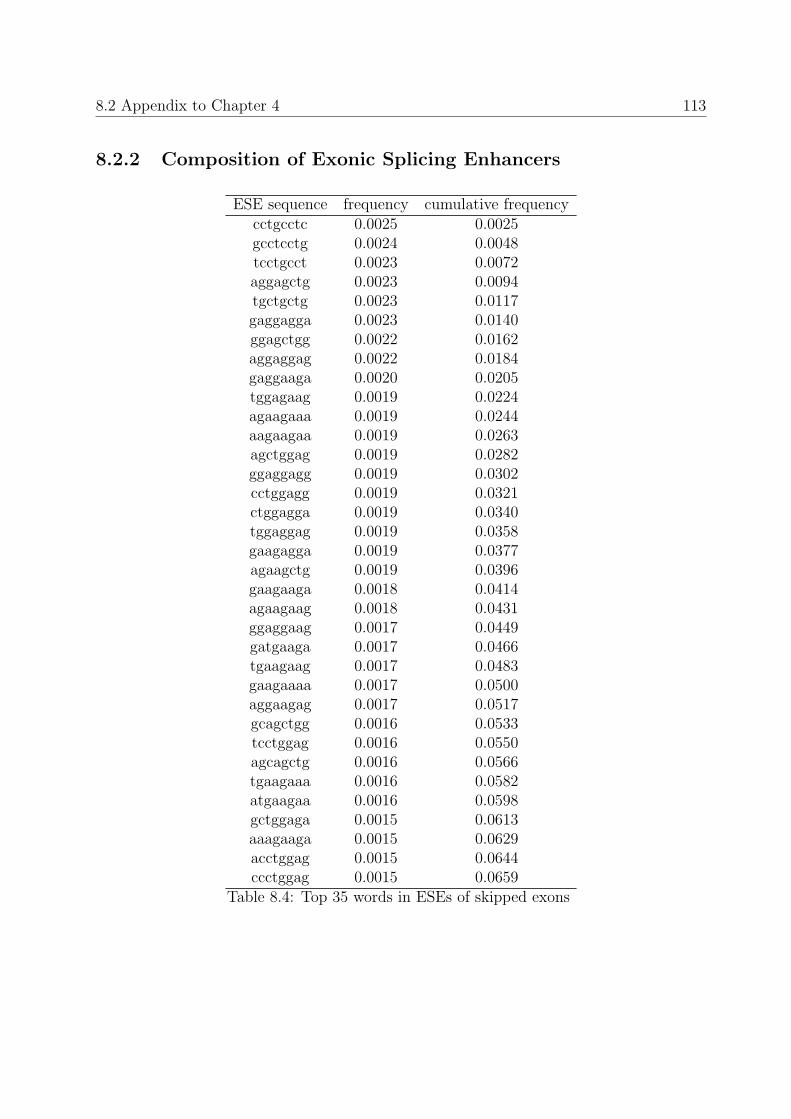
8.2 Appendix to Chapter 4 113
8.2.2 Composition of Exonic Splicing Enhancers
ESE sequence frequency cumulative frequencycctgcctc 0.0025 0.0025gcctcctg 0.0024 0.0048tcctgcct 0.0023 0.0072aggagctg 0.0023 0.0094tgctgctg 0.0023 0.0117gaggagga 0.0023 0.0140ggagctgg 0.0022 0.0162aggaggag 0.0022 0.0184gaggaaga 0.0020 0.0205tggagaag 0.0019 0.0224agaagaaa 0.0019 0.0244aagaagaa 0.0019 0.0263agctggag 0.0019 0.0282ggaggagg 0.0019 0.0302cctggagg 0.0019 0.0321ctggagga 0.0019 0.0340tggaggag 0.0019 0.0358gaagagga 0.0019 0.0377agaagctg 0.0019 0.0396gaagaaga 0.0018 0.0414agaagaag 0.0018 0.0431ggaggaag 0.0017 0.0449gatgaaga 0.0017 0.0466tgaagaag 0.0017 0.0483gaagaaaa 0.0017 0.0500aggaagag 0.0017 0.0517gcagctgg 0.0016 0.0533tcctggag 0.0016 0.0550agcagctg 0.0016 0.0566tgaagaaa 0.0016 0.0582atgaagaa 0.0016 0.0598gctggaga 0.0015 0.0613aaagaaga 0.0015 0.0629acctggag 0.0015 0.0644ccctggag 0.0015 0.0659
Table 8.4: Top 35 words in ESEs of skipped exons

114 8 Appendix to chapters 2-6
ESE sequence frequency cumulative frequencygaagaaga 0.002698809 0.002698809aagaagaa 0.002564728 0.005263538agaagaaa 0.002355012 0.00761855tgaagaag 0.002275939 0.009894489agaagaag 0.002272501 0.012166989gaggagga 0.002176237 0.014343227aggaggag 0.002165923 0.01650915ctggagga 0.00212123 0.01863038agctggag 0.002117792 0.020748172gaagaaaa 0.002114354 0.022862526tggagaag 0.002093726 0.024956252tggaggag 0.00206966 0.027025912tgctgctg 0.002062784 0.029088696ctggagaa 0.002028405 0.031117101gatgaaga 0.002021529 0.033138629aggagctg 0.002014653 0.035153282tgaagaaa 0.001945893 0.037099175atgaagaa 0.001921827 0.039021003gaagatga 0.001897762 0.040918764agcagctg 0.001894324 0.042813088ctgaagaa 0.001877134 0.044690221aggagaag 0.001863382 0.046553603ggagctgg 0.001825564 0.048379167gaggaaga 0.001822126 0.050201293agaagctg 0.001808374 0.052009668ggaggagg 0.00179806 0.053807728gaagagga 0.00179806 0.055605788aaagaaga 0.00179806 0.057403848ggagaaga 0.001773994 0.059177843cctggaga 0.001701797 0.06087964cagaagaa 0.001701797 0.062581437agaagatg 0.001684607 0.064266044agaaggag 0.001653665 0.06591971gctggaga 0.001636476 0.067556185cctggagg 0.001626162 0.069182347
Table 8.5: Top 35 words in ESEs of constitutive exons

8.2 Appendix to Chapter 4 115
8.2.3 Exons with intronic properties
Figure 8.1: Exons with intronic properties: Dinucleotides
Figure 8.2: Exons with intronic properties: Triplets
8.2.4 Transformations from ESE to ESS

116 8 Appendix to chapters 2-6
Figure 8.3: Exons with intronic properties: 4-mers
Figure 8.4: Transformation: Distances to the ESE and ESS words
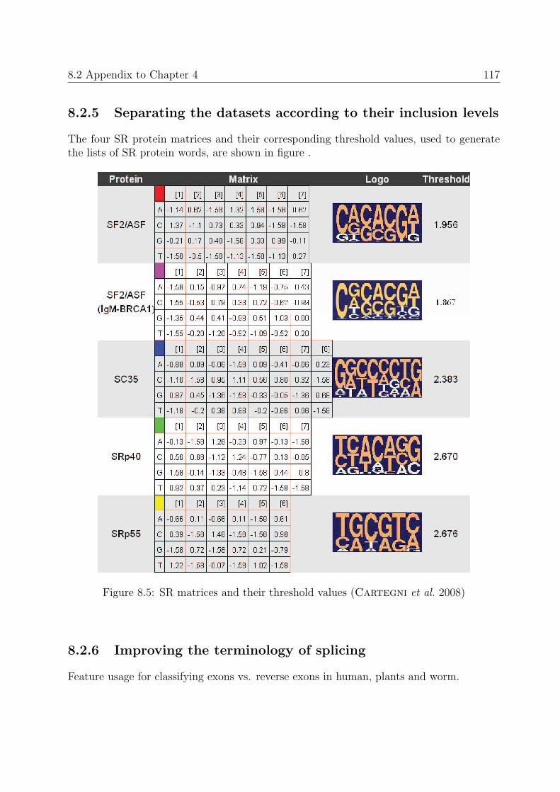
8.2 Appendix to Chapter 4 117
8.2.5 Separating the datasets according to their inclusion levels
The four SR protein matrices and their corresponding threshold values, used to generatethe lists of SR protein words, are shown in figure .
Figure 8.5: SR matrices and their threshold values (Cartegni et al. 2008)
8.2.6 Improving the terminology of splicing
Feature usage for classifying exons vs. reverse exons in human, plants and worm.

118 8 Appendix to chapters 2-6
Table 8.6: Unified description of splicing data
Species: HumanMethod: AltSplice: EST/cDNA to genome alignmentsSource: EST/cDNA
Conservation: No conservation limitationProtein coding: No protein coding limitation
Frame preserving: No frame preserving limitationStop codon: Yes
Exon rank in transcript: Middle exonsEST-tissue: All ESTs
Constitutive: 2 ESTsSpecial issues: No special issues
Figure 8.6: Feature usage for classifying exons vs. reverse exons in human, plants andworm.

8.3 Appendix to Chapter 5 119
8.3 Appendix to Chapter 5
Figure 8.7: Ratios between different nucleotides within exons
8.4 Appendix to Chapter 6

120 8 Appendix to chapters 2-6
Figure 8.8: Distributions of ratios between different nucleotides within exons

8.4 Appendix to Chapter 6 121
Figure 8.9: ESE densities after adjustment of model 5: A close overlap of the two densitycurves could be reached
Figure 8.10: ESE densities on cleaned constitutive data versus m8 s.exons

122 8 Appendix to chapters 2-6
Figure 8.11: ESE-networks: the co-occurrence patterns on each two ESE motifs are similarbetween the top 300 words in exons, s.exons and the top 100 words on SCE data

8.4 Appendix to Chapter 6 123
Figure 8.12: The normalized distances of the ESE networks are similar between constitutiveexons and randomly shuffled m2 s.exons

124 8 Appendix to chapters 2-6
Figure 8.13: Constitutive s.exons: Densities of different SR-proteins and different ESE-and ESS collections
Figure 8.14: Constitutive s.exons: Densities of different SR-proteins and different ESE-and ESS collections on s.exons with removed stop-codons

8.4 Appendix to Chapter 6 125
Figure 8.15: SCE s.exons: Densities of different SR-proteins and different ESE- and ESScollections
Figure 8.16: 61 mutations at acceptor splice sites between human and mouse

126 8 Appendix to chapters 2-6
Figure 8.17: Mutations at acceptor splice sites between human, chimp and mouse
Figure 8.18: Mutations at acceptor splice sites of 297 constitutive introns vs. alternativein mouse

Eidesstattliche Erklarung
”Ich versichere, dass ich die von mir vorgelegte Dissertation selbstandig angefertigt, diebenutzten Quellen und Hilfsmittel vollstandig angegeben und die Stellen der Arbeit - ein-schließlich Tabellen, Karten und Abbildungen -, die anderen Werken im Wortlaut oderdem Sinn nach entnommen sind, in jedem Einzelfall als Entlehnung kenntlich gemachthabe; dass diese Dissertation noch keiner anderen Fakultat oder Universitat zur Prufungvorgelegen hat; dass sie - abgesehen von unten angegebenen Teilpublikationen - noch nichtveroffentlicht worden ist sowie, dass ich eine solche Veroffentlichung vor Abschluss desPromotionsverfahrens nicht vornehmen werde. Die Bestimmungen der Promotionsord-nung sind mir bekannt. Die von mir vorgelegte Dissertation ist von Prof. Dr. ThomasWiehe betreut worden.”

Lebenslauf
Name Ivana VukusicGeburtsdatum 1.4.1979Geburtsort BelgradFamilienstand ledigStaatsburgerschaft deutsch
Universitatslaufbahn10.2004-heute Universitat zu Koln, Institut fur Genetik
Promotionsstudentin am Lehrstuhl fur Bioinformatik4.2005-7.2005 CUBIC: Post-Graduate Course in Bioinformatics,
Basics in Biosciences, Univesitat zu Koln10.1998-08.2004 Informatik und Betriebswirtschaftslehre (Nebenfach)
an der Universitat Dortmund. Schwerpunkte:Genetische Programmierung, Bioinformatik
Stipendien10.2006 Reise-Stipendium fur die ISMB in Fortaleza, Brasilien
Schulbildung06.1998 Abitur, Leistungskurse Englisch und Mathematik08.1990-06.1998 Gymnasium in Brilon01.1990-06.1990 Gymnasium in Hilden09.1985-01.1990 Grundschule in Belgrad
SprachkenntnisseDeutsch (Muttersprache)Serbokroatisch (Muttersprache)Englisch (sehr gute Kenntnisse in Wort und Schrift)Italienisch (Schulkenntnisse)Latein (großes Latinum)
InteressenBioinformatik, GP, Schach (mehrmalige DeutscheMeisterin beim Jugend-Mannschaftsspiel), Computer,Standard- und Latein-Tanz, Stadtereisen, Lesen