Journal of Computational Neuroscience 6, 5–26 (1999)c© 1999 Kluwer Academic Publishers. Manufactured in The Netherlands.

Signals in Stochastically Generated Neurons

JAMES L. WINSLOW AND STEPHAN F. JOUPhysiology Department and Institute of Biomedical Engineering, University of Toronto, Toronto, Ont. M5S 1A8

winslow@spine.med.utoronto.ca

SABRINA WANG AND J. MARTIN WOJTOWICZPhysiology Department, University of Toronto, Toronto, Ont. M5S 1A8

Received July 10, 1997; Revised February 10, 1998; Accepted February 17, 1998

Action Editor:

Abstract. To incorporate variation of neuron shape in neural models, we developed a method of generating apopulation of realistically shaped neurons. Parameters that characterize a neuron include soma diameters, distancesto branch points, fiber diameters, and overall dendritic tree shape and size. Experimentally measured distributionsprovide a means of treating these morphological parameters as stochastic variables in an algorithm for productionof neurons. Stochastically generated neurons shapes were used in a model of hippocampal dentate gyrus granulecells. A large part of the variation of whole neuron input resistanceRN is due to variation in shape. Membraneresistivity Rm computed fromRN varies accordingly. Statistics of responses to synaptic activation were computedfor different dendritic shapes. Magnitude of response variation depended on synapse location, measurement site,and attribute of response.

Keywords: stochastic neurons, dendrites, synapse location, hippocampus, membrane resistivity

1. Introduction

Simulations of biological neural networks require ge-ometry of neurons. Dye filling and tracing of neurons isa time-consuming process, particularly if serial recon-struction is involved. Typically biologically realisticsimulations are performed on one or two reconstructedgeometries (e.g., Jonas et al., 1993; deSchutter andBower, 1994a, 1994b). This is an insufficient numberof cell shapes when the effects of geometry and sourcesof variation are considered. Alternatively, arrays ofneurons with all the same shape per type of neuron areused in network simulations (e.g., Traub and Miles,1991; Wilson and Bower, 1989; Manor et al., 1997).To address this undersampling problem, a populationof cell shapes is required for a particular type of neu-ron. If these shapes are sufficiently realistic—that is,

if the population of generated cell shapes (statistically)looks and behaves like a population of neuron shapes—then this provides a method for addressing two typesof problems. First, this approach can be used to ana-lyze sources of variation of parameter measurementsand signal responses due to natural variation of neu-ron shape. Second, to analyze interaction of functionalgroups of neurons in a biological neural network, onecould generate shapes per type of neuron and distribu-tions of synaptic connections. This would incorporatestochastic variability of neuronal shapes and connec-tions with existing methods of single neuron compu-tations to model interaction of many neurons. In bothtypes of problems, analysis of variation in response dueto variation in neuron shape is addressed.

We have developed an algorithm for generating apopulation of stochastic neurons from a data set of

6 Winslow et al.

neurons, whose distributions of morphological featureshave been measured or can be approximated. A prob-lem of the first type is then addressed using the tech-nique of stochastic neurons. The extensive and detailedanalysis of signals in single neurons provides a com-parison and is augmented by this strategy.

We used this approach to analyze responses of hip-pocampal dentate gyrus (DG) granule neurons to stim-ulation of different parts of the perforant pathways. Inthe hippocampus, the extrinsic afferents to the den-tate gyrus have entorhinal, hippocampal, hypothala-mic, septal, and brainstem origins (Cowan et al., 1980;Witter, 1993). Of these, the most important pathway,quantitatively and perhaps functionally, is formed bythe axons that arise from the medial and lateral partsof the entorhinal cortex. These projections constitutethe perforant pathway, which is divided into the lateraland medial perforant pathways (LPP and MPP), andform part of the intrinsic circuitry of the entorhinal-hippocampal system. The axons in LPP originate fromneurons in the lateral entorhinal cortex and preferen-tially synapse onto the distal third (with respect to thesoma) of dendrites in the molecular layer. In contrast,the MPP projects from the medial entorhinal cortexand preferentially synapses onto the middle third ofthe dendrites. Electrophysiological responses of gran-ule neurons to the activation of the two pathways havebeen described extensively (Wang et al., 1996; Wangand Wojtowicz, 1997).

We computed the voltage signals within the somaand dendritic tree of the stochastically generated DGneurons, after discretizing the dendritic trees into elec-trical compartments at high resolution to preserve ge-ometry (Rall, 1959; Hines, 1989; Winslow, 1990).While it is now technically possible to experimentallyrecord these signals (Stuart and Sakmann, 1994), thishas been done only in neurons that are easier to accessand record than the DG neurons. The simulation re-sults presented here provide results that are currentlynot (easily) attainable in a biological preparation.

We compared properties of soma excitatory post-synaptic potentials (EPSPs) from the experiments withsimulations on different neuronal shapes in the stochas-tically generated population and with predictions fromcable theory of dendrites (Rall, 1964; Rall et al., 1992;Holmes, 1989). Although voltage activated channelshave been reported and theoretically analyzed (Stuartand Sakmann, 1994; Cook and Johnston, 1997), wefirst resolved signals in stochastic neurons with pas-sive membrane. We also commented on values ofRm

computed from whole neuron resistanceRN in termsof variation in geometry of neurons. We found thatsome parameters depend strongly on the shape of den-dritic trees while others do not. Preliminary electro-physiological data determined that some aspects of thecomputed synaptic responses varied in accordance withexperimental data obtained by stimulation of LPP andMPP in the hippocampal slice preparation.

Initial results of this work have been published inabstract form (Jou et al., 1995).

2. Methods

2.1. Stochastic Generation of Cell Shapes

A typical dendritic tree traced from a Lucifer Yellow-filled granule neuron in a hippocampal slice prepara-tion is shown in Fig. 1 (see Section 2.4 for details).The algorithm for stochastic generation of cell shapesuses the probability distributions of various shape char-acteristics observed in granule cells. For example, thesoma is approximated by a prolate ellipsoid with lengthof 18.6± 3.43µm (mean± standard deviation) and awidth of 10.3± 2.06µm (Claiborne et al., 1990). As-suming that the soma length and width are each nor-mally distributed (for lack of further data), then a newsoma can be generated by simply choosing a randomnumber from a normal distribution of mean 18.6 and

Figure 1. Representative reconstructed image of a Lucifer Yellow–filled DG granule cell (DG) neuron from a hippocampal slice prepa-ration. This cell has been used for quantitation of the dendritic tree(traced shape included in Table 4). Asterisks indicate branches thatdid not appear to be completly filled with the dye and were arbitra-rily extended toward the fissure of the molecular layer. Scale bar:100µm.

Stochastic Neurons 7

Table 1. Probability distributions used to generate DG granulecells are the specific distributions used in the implementation ofthe shape-generation algorithm. In the branch point distribution,fB(ω), ω is the normalized distance of a branch point from thesoma, whereω= 0 is at the some andω= 1 is at the distal tips ofthe dendritic tree (at the fissure). Equation (1) in the text gives thevalues for fB(ω). The noise distribution is a function applied tothex andy coordinates of points along the dendrite to approximatedendritic wiggle, the small turns and deviations which a dendriteexhibits (see text). Starred distributions (*) are based on data fromClaiborne et al. (1990), where the standard deviations were com-puted from the standard error values given in the reference. Notethat all dendrites were assumed to terminate at 300µm.

Item Distribution mean± sd

Soma length* Normal 18.6± 3.43µm

Soma width* Normal 10.3± 2.06µm

Number of primary dendrites* Normal 1.9± 1.37

Number of branch points* Normal 13± 2.97

Branch point location* Staircase fB(ω)

Tree height Constant 300µm

Transverse spread* Normal 325± 75.4µm

Longitudinal spread* Normal 176± 41.1µm

Noise distribution Normal 0± 1µm

standard deviation 3.43 for its length inµm, and asecond random number from a normal distribution ofmean 10.3 and standard deviation 2.06 for its widthin µm. A random variate from a normal distributioncan be generated using the standard Box-Muller algo-rithm (Press et al., 1992, sec. 7.2). A population ofsoma shapes generated in this manner should have thesame distribution of lengths and widths as actual somashapes. This same principle of using probability dis-tributions based on biological observations from realrat granule cell dendritic trees can generate a dendritictree. The distributions that we used are given in Table 1.

2.2. The Algorithm

A dendritic tree is comprised of connected branch seg-ments, situated between branch points and end pointsin three dimensions. Generating the dendritic tree in-volves six steps: (1) generating the branch point nor-malized distances, (2) connecting the branch points toform a one-dimensional projected tree, (3) mapping theone-dimensional projected tree to a three-dimensionaltree, (4) scaling the normalized coordinates to real coor-dinates, (5) adding dendritic diameters, and (6) addingdendritic wiggle (see Fig. 2).

2.2.1. Generating the Branch Point Locations.Thebranch points{b1, b2, . . . ,bnB} are first generatedin normalized coordinatesbi = (χi , ψi , ωi ) and thenscaled to actual coordinates(xi , yi , zi ). A branch pointlocation distribution fB(ω) describes the probabilityof a branch point occurring at normalized distanceωwithin the stratum moleculare, whereω= 0 is at thesoma in stratum granulosum andω= 1 is at the hip-pocampal fissure where the granule cell dendrites ter-minate (Claiborne et al., 1990). This distribution fol-lows directly from experimental observations of branchpoints. For example, the branch point probability dis-tribution of Table 1 is

fB(ω) =

0.63, 0≤ ω ≤ 1/3,

0.27, 1/3< ω ≤ 2/3,

0.10, 2/3< ω ≤ 1,

(1)

which means that 63% of the branch points occur (uni-formly distributed) within the proximal third of thestratum moleculare or dendritic tree, 27% uniformlywithin the middle third, and 10% uniformly within thedistal third.

First, choose the number of branch pointsnB follow-ing the experimentally observed distribution in Table 1.In general, the probability distribution of branch pointnormalized distances can take on almost any form. Sec-ond, the branch point normalized distancesωi are gen-erated for any arbitrary probability distributionfB(ω)

as follows. Choose random variatesu1, u2, . . . ,unB

from a uniform random distribution on [0, 1] gener-ated using the Park-Miller algorithm (Press et al., 1992,sec. 7.1). Then apply

ωi = F−1B (ui ); i = 1, . . . ,nB, (2)

whereFB(ω) is the cumulative density function corre-sponding tofB(ω).

Probability[ωi ≤ ω] = FB(ω) =∫ ω

−∞fB(t) dt

=∫ ω

0fB(t) dt, (3)

where 0≤ ω ≤ 1 andF−1B (ω) is its inverse. It can be

shown by graphical plots offB(ω) versusω andFB(ω)

versusω that the frequency distribution of the set ofωi

points resulting from Eq. (2) isfB(ω). Thus, the valuesof the normalized distances from the soma of the gen-erated branch points will behave like the experimentalobservations.

8 Winslow et al.

Figure 2. Steps in the algorithm to generate a normalized dendritic tree. Details in text. A: The generated branch pointsbi = (0, 0, ωi );i = 1, . . . ,nB, where theωi are values of normalized distances from the soma shown on the vertical axis (ω = 0 at soma andω = 1 at bottom).B: Connected branch points to form a 1D collapsed tree. The connections have been expanded slightly so that they are visible; in actuality, allthe branch points are still collinear on a single axis underneath the soma, as in the previous step. C: Expanded 1D tree to form a 3D tree, wherethe branch points arebi = (χi , ψi , ωi ).

Preliminary to connecting the branch points, sort theωi -values so thatω1 ≤ ω2 ≤ · · · ≤ ωnB . Let the branchpoints bebi = (0, 0, ωi ) for i = 1, . . . ,nB (Fig. 2A).

2.2.2. Connecting the Branch Points to Form a 1DProjected Tree. A branch point by definition repre-sents a point in space where a singleparent dendritebranches into two child dendrites. The point at the dis-tal tip is called anend point. If one assumes that thedendritic tree always extendsoutward from ω = 0to ω = 1, then it is possible to connect the branchpoints and end points together in an unambiguous man-ner to produce a connected tree. At this stage, thebranch points are projections on the normalizedz-axis(ω-axis).1

The branches are connected as follows. Choose thenumber of primary branchesnP, again drawing froman experimentally derived distribution (Table 1). Cre-atenP parent segments (primary segments), connect-ing the soma to branch pointsb1, . . . ,bnP . Then foreachbi , create two child segments betweenbi and thenext two distal pointsbj andbj+1, wherei < j , whichdo not already have parent dendrites. If no such branchpoint exists, then create an end point atω = 1 and con-nect a child segment to it.

The resulting set of dendritic segments produces aconnected tree with the desired characteristics. Sinceωi ≤ω j for i < j and all distal branch end points are lo-cated at normalized distance 1, connections are alwaysmade for increasingω, and all the segments will extendin a proximal-to-distal direction. Since connections arealways made to the next two distal (most proximal un-connected) points, it is guaranteed that each connectedbranch point always has one parent and two child den-dritic segments. Finally, since this process is done forall branch points in the setB, no branch point is leftunconnected (Fig. 2B).

2.2.3. Mapping the 1D Projected Tree to a 3D Tree.This step may be thought of as expanding the genera-ted (projected onω-axis) tree into a 3D tree by assign-ing normalizedχ andψ coordinates to each branchpoint.

First assign(χ, ψ) coordinates to the end points suchthat they project inside a circle of radius 1. Four endpoints are assigned values of(−1, 0), (1, 0), (0, −1),and(0, 1). The remaining end points are distributedrandomly within the unit circle by generating pairs ofuniform random numbersχ,ψ within [−1, 1] and ac-cepting the pair only ifχ2+ ψ2 ≤ 1.

Stochastic Neurons 9

For each of the remaining points, which are allbranch points, their(χ, ψ) values are assigned the av-erage values of the distal end points of the two childbranches to which it is connected. That is, if thetwo distalward segments ofbi connect to(χ1, ψ1) and(χ2, ψ2), then (χi , ψi ) of bi is set to((χ1+χ2)/2,(ψ1+ψ2)/2).

2.2.4. Scaling the Normalized Coordinates to ActualCoordinates. An actual distanceH is chosen for thedendritic tree from the height distribution (Table 1),which in this case is constant. Then settingzi = Hωi

for i = 1, . . . ,nB scales the normalized distances toactual distances from the soma.

Longitudinal and transverse spreadsl treeandttreearechosen for the tree from the experimental distribution(Table 1). Scale the unit circle that contains the endpoints onto an ellipse with diametersl treeandttreeby set-ting x= 1

2l treeχ andy= 12ttreeψ . This produces a spa-

tial arrangement of the dendritic tips consistent with theexperimental observation that the widest spreadttree ofthe tips occurs in the transverse plane of the hippocam-pus and perpendicular spreadl tree in the longitudinalplane (Claiborne et al., 1990). Thus, the set of points{bi ; i = 1, . . . ,nB}, where

bi = (xi , yi , zi ) =(

1

2l treeχi ,

1

2ttreeψi , Hωi

),

are the actual 3D coordinates of a full dendritic tree(Fig. 2C).

2.2.5. Adding Dendritic Diameters. Each dendriticsegment length was divided by the smallest integersuch that the size of a compartment is≤1 µm, andeach compartment assigned a diameter based on thedistance of the compartment’s midpoint and using thedendritic diameter versus distance functionKdiamd(z)obtained from the electron micrograph measurementsdescribed below. The length of each compartment iswell within 10% of the space constant for a granule neu-ron, so that numerical accuracy of the compartmentalsimulations can be assured. Since dendritic diameteris taken to only be a function of distance on thez-axis(not radial from soma or arc length on branch), twochild branches at a branch point have the same initialdiameter but can taper at different rates, depending onthe angle of branching, with respect to thez-axis, orthe derivative∂d/∂z as function ofz. Since we donot have sufficient data to take into account a correla-tion between soma size and initial dendritic diameter,

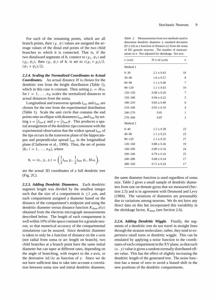
Table 2. Measurements from two methods used todetermine dendritic diameter± standard deviation(D± sd) as a function of distance (z) from the somaof DG granule neurons. The number of measure-ments inn. Not adjusted for shrinkage. See text.

z (µm) D± sd(µm) n

Method 1

0–30 2.1± 0.63 10

30–60 1.6± 0.57 8

60–90 1.1± 0.40 7

90–120 1.1± 0.63 10

120–150 0.98± 0.26 7

150–180 0.94± 0.22 5

180–210 0.85± 0.49 6

210–240 0.95± 0.10 4

240–270 0.81 1

270–300 0.87 2

Method 2

0–40 1.2± 0.38 23

40–80 1.1± 0.23 23

80–120 1.1± 0.32 27

120–160 0.88± 0.26 19

160–200 0.89± 0.16 24

200–240 0.79± 0.16 25

240–280 0.68± 0.24 17

280–320 0.71± 0.24 17

the same diameter function is used regardless of somasize. Table 2 gives a small sample of dendritic diame-ters from one rat dentate gyrus that we measured (Sec-tion 2.5) and is in agreement with Desmond and Levy(1984). The variations of diameters are presumablydue to variations among neurons. We do not have anydirect data on this but incorporated this variability inthe shrinkage factor,Kdiam (see Section 2.6).

2.2.6. Adding Dendritic Wiggle. Finally, the seg-ments of a dendritic tree do not travel in straight linesthrough the stratum moleculare; rather, they tend to ex-perience small turns or dendritic wiggle. This can beemulated by applying a noise function to the coordi-nates of each compartment in the XY plane, so that each(x, y) value is given a random normally distributed off-set value. This has the effect of slightly increasing thedendritic length of the generated tree. The noise func-tion has a mean of zero to avoid a biased shift in thenew positions of the dendritic compartments.

10 Winslow et al.

2.3. Implementation of Algorithm

A program that implements this algorithm and usesthe distribution functions listed in Table 1 was writ-ten using ANSI C. To ensure uniformity across differ-ent versions of C, uniform and normal random num-ber generation routines were also written. Uniformlydistributed random numbers were generated using thePark-Miller algorithm with a Bays-Durham shuffle,and normally distributed numbers were generated usingthe Box-Muller method (Press et al., 1992). Each gen-erated shape is assigned an integer number, which alsoserves as the seed for the random number stream. Thisgives each shape a unique identifying number and pro-vides a convenient way to reproduce uniquely an entiregenerated shape from a single number. The programtakes a shape number and a value forKdiam and pro-duces the corresponding generated shape. A montageof representative generated shapes is shown in Fig. 3.The program, as implemented, can generate a singlenovel complete granule cell shape in≤10 s on a Sun 3workstation.

2.4. Digitization of Filled DG Granule Neurons

A DG granule neuron was filled with Lucifer Yellowand photographed onto a slide and traced (Fig. 1).The photographic negative was video digitized us-ing an instrumentation video camera (NC-70, Dage-MTI, Inc., Michigan City, IN 46360) and a Win-TVboard (Hauppauge Computer Works, Inc., Hauppauge,NY 11788) on a PC with a program running underDOS (Winslow, 1994). The digitized images weretransferred to a Silicon Graphics Indigo computer(Silicon Graphics, Inc., Mountain View, CA 94039-7311), where the scale bar and the nodes and branchesof the tree were traced using a tree tracing program(Winslow, 1995). Details on the hardware, data struc-tures, and algorithms used have been described previ-ously (Winslow et al., 1987).

Similar to the representative traced granule neuronshown in Fig. 1, the extent of the dendrites gave agood indication of the location of the hippocampal fis-sure when the original stained cell is viewed in theslice preparation. The dendrites appeared to terminatealmost completely at the fissure, consistent with ob-servations by others (Claiborne et al., 1990). Threedendrites seemed to disappear before reaching the fis-sure, but they also gradually faded out from the im-age, likely as a result of projecting above or below the

Figure 3. Six representative generated shapes. Shapes such as thesewere computer-generated using the stochastic algorithm described inthe main text. A shape can be uniquely identified and reproducedfrom a single ID number, which serves as the random number streamseed. Images were generated from the output geometry files usinga ray tracer. Clockwise from the upper left: shape 30, 7, 2, 22, 1,and 6.

focal plane. Given that nearly all granule neuron den-drites terminate at the fissure or the pial layer, when theneuron was traced, those dendrites that faded out pre-maturely were extended by eye in the construction ofthe traced shape model. A total of three dendritic seg-ments were extended, adding only 247µm of dendriticlength to the tree, for a total dendritic length of 3380µm. The traced shape had 30 dendritic segments, threeprimary branches, and a longitudinal spread of 404µm.These values agreed well with published values on re-constructed granule cells (Table 4). In particular, thedendritic length of this granule cell from a immature(21-day-old) rat agreed well and was even slightlyhigher than the average dendritic length of an adultrat granule cell. This is consistent with the observationthat at three weeks after birth the dendritic arborization

Stochastic Neurons 11

of granule neurons is the same as in adult cells (Cowanet al., 1980), although spine development is not yetfully mature (Cotman et al., 1973; Crain et al., 1973).Therefore, a branch point distribution based on granuleneuron dendritic trees in adults can still be used to gen-erate trees in younger, 15- to 30-day-old rats, althoughadult measurements of spine sizes and densities cannotbe used without appropriate scaling.

2.5. Measurement of Dendritic Diameters

To complete the statistics for dendrites, diametersare required. Transverse hippocampal slices from a35-day-old rat were prepared with standard methodsfor electrophysiological experimentation (Wang et al.,1996). For electron microscopy examination, 400µmslices were fixed in 6.2% glutaraldehyde in 0.1 Msodium cacodylate buffer (pH 7.4) containing 0.011%CaCl2 and 4% sucrose. After rinsing in buffer, the tis-sue was postfixed in 2% osmium tetroxide, dehydratedin ethanol, embedded in epoxy, and sectioned on a Re-ichert “Ultracut” microtome.

Since the long axis of the dendritic tree is approx-imately perpendicular to incoming axons of the per-forant pathway, thin sections (75 nm) were cut in aplane parallel to the dendritic tree and the incoming per-forant pathway, so as to facilitate recognition and mea-surement of the dendritic profiles. Dendritic brancheswere distinguishable from axons and other cells in theneuropil since they appeared mainly in longitudinal oroblique view, lacked synaptic vesicles, and were gen-erally more electronlucent. Four consecutive sectionswere micrographed using a Hitachi H-7000 transmis-sion electron microscope.

• Method 1 In five separate fields, diameter measure-ments were made of dendritic profiles that extendedlongitudinally or obliquely. Each field, which ex-tended from the cell body layer to the fissure of themolecular layer, was about 360 by 30µm. Measure-ments of 10 to 20 profiles from each field were madeby a naive observer. In cases where the diameter ofthe dendrite was not uniform along its length, it wasassumed that the dendrite had been cut obliquely toits long axis, so the smallest ellipsoid diameter (truediameter) was measured.• Method 2 The dendritic diameter measurements

were independently confirmed in another field froma different area of the same dentate gyrus by a differ-ent observer. A square grid (20×20µm per square)

was overlaid on each micrograph. Coordinates cor-responding to the squares were uniformly, randomlychosen with a density of approximately 24 samplesper micrograph (total area 43,000µm2). Within eachrandomly chosen square, a measurement of dendriticdiameter was made if a dendrite could be identifiedwithin the chosen sample. Dendrites were identifiedby (1) electronlucent, (2) presence of postsynapticdensity, (3) presence of mictrotubles, and (4) lack ofvesicles. The number of these identified features(one to four) per observed dendrite and diameterwere recorded. These values were used to computea weighted mean of diameters, so that diameters thatcame from unequivocal dendrites contributed moreto the mean than tenuously identified dendrites.

The results from these two methods were found notto differ significantly and are reported in Table 2. Theyare similar to those of Desmond and Levy (1984) ob-tained from adult animals. Using a generalized least-squares curve-fitting procedure, diameter as a functionof distance,z, from the soma within the dendritic layerwas best fit by

fd(z) = 1.713 exp(−z/47.70)+ 0.8626, (4)

where fd andz are inµm.We corrected for tissue shrinkage, which occurred

as a result of the chemical processing for electronmicroscopy (Hayat, 1981), by using a unitless scal-ing factor,Kdiam= Dt/Dm, whereDt = true diameter,Dm=measured diameter, andS= shrinkage= (Dt −Dm)/Dt . In the computation of passive parametersand the simulations,Kdiam was varied from between1.0 (S= 0) to 1.4 (S= 29%). The function

d(z) = Kdiam fd(z) (5)

is used in both the generated shapes and the tracedshape to set the dendritic diameters. Shrinkage of30 to 40%, including extracellular space, is expectedfrom the EM tissue preparation procedure (Hayat,1981). However, the exact shrinkage of the dendritesis not known and dendrites have lipid membranes,small cross-sections, and intracellular organelles, thusthey presumably shrink less. Consequently, we choseKdiam= 1.2 (S=17%).

2.6. Dendritic Spines

Up to 50% of the dendritic surface membrane may beattributed to the presence of dendritic spines (Hama

12 Winslow et al.

Figure 4. Local voltage responses to synaptic conductance placed on the different types of spines. The spine was located on the medial regionof the dendritic tree at 200µm from the soma in generated cell shape #49. A: An expanded spine, SPE. B: A simple spine, SP. C: No spine withdendritic shaft only for comparison.

et al., 1989), which are small, fingerlike protrusionsextending from the dendrites of many neurons andoften, but not always, terminating in bulbous expan-sions (Fig. 4). They increase the effective surface area,thereby increasing the electrotonic length of dendriticsegments and electrotonically distancing the synapsefrom the soma (Holmes, 1989; Stratford et al., 1989;Holmes and Levy, 1990; Holmes and Rall, 1992; Segevet al., 1992; and discussion in Rall et al., 1992). Giventhe large number of spines on a single granule neu-ron, explicit creation of one or two compartments perspine on the dendritic tree generates a large numberof compartments requiring more equations and time-consuming simulations. Using the technique of Major(1992), we represented the spines on each dendriticsegment by increasing the length and diameter of thesegment and replacing the spiny dendrite with a singlelonger and wider smooth (spineless) dendrite.

The surface area contribution of spines was assumedto beKspineA µm2 per 1µm of dendrite (arc length),where A = 4.180, 2.806, 2.401µm2 for the proxi-mal, middle, and distal portions, respectively, of thestratum moleculare (Hama et al., 1989, Table 3).Kspine

is the scaling parameter that was introduced to addressthe uncertainty regarding the actual spine density andsize on granule neurons of immature rats. Immaturespines are not as large or elaborate and do not appearat the same densities as adult spines (unpublished ob-servation). We scaled down the adult spine estimatesby Kspine, where Kspine< 1 is interpreted as model-ing smaller, less elaborate, and less densely distributedspines.Kspine= 0.5 means the spine surface areas arehalf that of the adult spine surface areas as measuredby Hama et al. (1989). The simulated cells have halfthe number of spines as an adult rat granule neuron(Desmond and Levy, 1985) or the full adult number ofspines, but each spine has half the adult surface area.More likely, there is a combination of both smallerand fewer spines in the simulated immature rat granuleneuron compared with an adult.

Our data are based on six dendritic segments (threefrom lateral and three from medial perforant pathway)with a total length of 10.7µm. All these segmentswere fully reconstructed from serial EM sections. Wecounted 35 synapses contacting the dendrites and onlyfive contacting spines. All spines were very small,

Stochastic Neurons 13

Table 3. Parameters used in the simulations. Thespine values are based on adult-sized rat DG granuleneurons (Hama et al., 1989). Each linear parameter isscaled byK 1/2

spine, so that the final surface area of all thespines is scaled by a factor ofKspine. See text.

Parameter Value

α 0.5

1t 0.25

Cm 0.7µF/cm2

gmax 0.45 nS

Kspine 0.5

Kdiam 1.2

Ri 150Ä cm

Rm 78.3 KÄ cm2

Vrest −69.8 mV

Compartment length ≤1µm

Spine Area µm2/µm dendrite lengthProximal third Kspine4.180

Middle third Kspine2.806

Distal third Kspine2.401

SPE Spines

Head Height K 1/2spine0.51µm

Head diameter K 1/2spine0.50µm

Base height K 1/2spine0.752µm

Base diameter K 1/2spine0.185µm

SP Spines

Base height K 1/2spine1.253µm

Base diameter K 1/2spine0.333µm

Tip diameter K 1/2spine0.258µm

measuring 0.5 to 1µm in length and diameter. Twoother spinelike projections were devoid of synapses.Seven spines per 10.7µm of the dendritic lengthamounts to 0.65 spines/µm, a much smaller spine den-sity than the reported 1.4 spines/µm in adult animals(Desmond and Levy, 1985), consistent with our esti-mate ofKspine = 0.5. To implement this, we wrotea program that takes a dendritic tree shape (such asthe traced shape or a generated shape) and for a givenvalue ofKspine calculates the spine-collapsed version.For most of the simulationsKspine= 0.5 was used.

2.7. Shape to Compartments

The 3D description of a dendritic tree has the formof a list of xyzcoordinates of locations of the soma,

branch points, and distal tips. This representation givesthe visual lifelike shape and exact shape measure-ments, which are then the data used for the shape statis-tics. The dendrite is discretized into compartments,whereby each branch point and dendrite end points arecenters of compartments, and each branch is subdi-vided into compartments. Because the structure is in3D, the true lengths of branches must be calculatedfrom the 3D distance between branch points.

The discretized neuron, when represented by com-partments for simulation, is a list of tuples, one percompartment, consisting of compartment number,compartment location, compartment parameters, list ofcompartments to which it connected, and input synapsenumber.

2.8. Simulation of Synaptic Potentials

A set of 50 different cell shapes was generated and con-verted into compartmental models. The compartmentsassigned in generating the neuron were used for thesimulations. Thus, the minimum and maximum com-partment lengths are 0.5 and 1.0µm, respectively. Theaverage number of compartments per simulation wasat least 3,430, which corresponds to the total lengthof the generated dendritic tree. All computer simu-lations were done using NEURON 2.0 (Hines, 1984,1989) on either a SUN-3 running BSD Unix or an In-tel 486DX33 PC running Linux. Simulation parame-ters are given in Table 3. When an activated synapsewas on a spine, these spines were explicitly modeled,using one or two compartments with the dimensionsgiven in Table 3, with spine measurements from Hamaet al. (1989). The remaining spines were implicitlyrepresented in the simulations, using the spine collapseprocedure. The time course of synaptic conductancewas simulated by theα function,gmax(αt) exp(1−αt),whereα = 0.5 andgmaxwere chosen, so that simulatedresponses at the soma had shape and amplitude similarto those of recorded responses in granule cells.

2.9. Electrophysiological Recordingsin Hippocampal Slices

Recordings and analysis of synaptic responses were de-scribed in our recent publications (Wang et al., 1996;Wang and Wojtowicz, 1997). All recordings were per-formed from cell bodies of the granule neurons in thewhole-cell configuration. Input resistances were mea-sured by applying 10 mV, 100 ms depolarizing voltage

14 Winslow et al.

steps from a resting membrane potential (approxi-mately−70 mV) and measuring steady-state currents.Synaptic responses were evoked at 0.1 Hz by electricalstimulation of afferent axons in the outer (LPP) andmiddle (MPP) molecular layers. Stimulus current wasadjusted to produce approximately equal amplitudesof evoked excitatory potentials (EPSPs) from LPP andMPP, as recorded in the cell body.

3. Results

3.1. Verification of the Algorithm

Verification of the algorithm, and overall correctnessof the program that implemented the algorithm, wasdone by ascertaining the realism and statistics of thegenerated shapes, of which a representative sample isshown in Fig. 3. Population statistics of tree measure-ments, some of which were not directly based on dis-tributions used in the algorithm, were computed on100 generated shapes, shapes 0 to 99. The number ofdendritic segments, number of primary branches, trans-verse spread, longitudinal spread, dendritic length, andtree shape (the ratio of longitudinal spread to trans-verse spread) were evaluated. These statistics for thegenerated shapes were then compared with those samestatistics published in the literature (Table 4).

The generated cell shapes appear to be realistic. Inall cases the mean statistics are comparable, imply-ing that on average the generated shapes are similar toactual cell shapes, at least with respect to the number ofdendritic segments, number of primary branches, trans-verse spread, longitudinal spread, dendritic length,

Table 4. Tree statistics comparing published values from actual DG granule neurons, computed values from thetraced shape, and computed values from 100 generated shapes. Published and generated shape values are± standarddeviation. Tree shape is the ratio of longitudinal spread to transverse spread. Longitudinal spread and tree shapefrom the traced shape is not available since it was projected on to a single plane. Note that the means of actual versusgenerated shapes are not significantly different. Published values are from Claiborne et al. (1990).

Characteristic Published values Traced shape Generated shapes

n 48 1 100

Dendritic segments 29± 6.86 30 25.8± 6.11

Primary branches 1.9± 1.39 3 2.41± 1.26

Transverse spread (µm) 325± 75.41 404 314± 66.8

Longitudinal spread (µm) 176± 41.13 — 177± 39.0

Dendritic length (µm) 3221± 535 3380.24 3430± 802

Tree shape 0.56± 0.21 — 0.54± 0.20

and tree shape. Further, the standard deviations of allthe statistics are also comparable. This suggests thatthe population of generated shapes also encapsulatesthe same variability expected in a population of realgranule cellsin vivo. Thus, we conclude that our algo-rithm and program, which implemented the algorithm,are valid for their purpose of generating this type ofneuron.

3.2. Passive Parameters

In addition to morphological details, the passive para-meters of granule neurons must be determined beforesimulations can be performed. The whole cell input re-sistanceRN = 280.4± 150.2 MÄwas measured exper-imentally in 320 granule neurons. This value is higherthanRN reported for adult rats (Staley et al., 1992) asmay be expected if the dendritic tree and soma weremore compact in our immature animals.

Given a value of axoplasmic resistivityRi , the pre-viously obtained measurement ofRN , and a specificcell shape (either the traced cell shape or a generatedshape), a unique value for membrane resistivityRm

may be computed using a recursive procedure. Insteadof using Ri , Rm and a given shape to computeRN

(Rall, 1957, 1989; Segev et al., 1989; Nitzan et al.,1990), we computed the theoretical value ofRm suchthatRN = 280.4 MÄ for each generated shape (Fig. 5).Because of recent evidence that the internal axoplas-mic resistivity Ri is actually much higher than previ-ously thought (Shelton, 1985; Jonas et al., 1993; Rappet al., 1994; Major et al., 1994; Thurbon et al., 1994;Borst and Haag 1996), computations were performed

Stochastic Neurons 15

Figure 5. A: Pathway to compute membrane resistivityRm. Given estimates of passive parametersRm andRi , and a cell shape, one can obtaina theoreticalRN from cable theory. In this article,RN was experimentally measured, andRi varied across a physiologically plausible range.Model geometries came from a tracing of an actual DG cell as well as from computer-generated shapes. B: Computed membrane resistivityRm

for generated and traced DG cell shapes, corrected for shrinkage. The dendritic diameters used in the shapes have been expanded to accountfor tissue shrinkage (Kdiam= 1.2). Points are theRi andRm values such that the measuredRN is 280.4 MÄ from young rat DG cells. Hollowshapes are for the traced shape; filled shapes are average values for 100 generated shapes. Triangles (upper curve):Kspine= 1.0, which givesspine surface areaKspineA = 4.180, 2.806, and 2.401µm2 perµm of dendrite for the proximal, middle, and distal thirds of the dendritic tree;squares (middle curve):Kspine= 0.75, giving KspineA= 3.135, 2.105, and 1.801µm2 perµm; circles (lower curve):Kspine = 0.50, givingKspineA = 2.090, 1.403, and 1.201µm2 perµm. The values corresponding toKspine= 0.50 are most appropriate for our young preparation.Bars are standard error.

from below the traditional value ofRi = 70Ä cm, toRi = 400Ä cm, which are generous bounds on the trueRi . Assuming tissue shrinkage factorKdiam= 1.2, theresults obtained are shown in Fig. 5B.

The nominal value ofCm used in the simulationswas 0.7µF/cm2, which is lower than the usual valueof 1.0µF/cm2 but is currently believed to be the mostaccurate value of membrane capacitance (Fettiplace

et al., 1971; Takashima and Schwan, 1974; Benz et al.,1975; Takashima, 1976; Haydon et al., 1980; Majoret al., 1994). However, ifCm is actually higher (e.g.,Borst and Haag, 1996), this will significantly alter thesimulated responses (see below). The predicted re-sponse will be more sluggish, with a slower rise time,lower amplitude, and longer time constant (not shown)and would not agree with our data.

16 Winslow et al.

Two agreements with theory may be seen at thispoint. First, the mean computedRm of our morpholog-ically realistic granule neurons, which were stochasti-cally generated, is very dependent on the surface areaof spines, as previously shown (e.g., Rall et al., 1992;Stratford et al., 1989; Holmes 1989; Holmes and Rall,1992; Segev et al., 1989). The standard deviations as-sociated with meanRm computed for differentKspine

values vary linearly with respect toKspine (3.0, 2.4,1.8 KÄ cm2 for Kspine= 1.00, 0.75, 0.50, respectively)but is constant with respect toRi (as shown in Fig. 5).The large differences in computedRm values due todifferent choices ofKspinemean that an accurate mea-surement of the spatial extent of spines is critical, if anexact determination ofRm is desired using this method.Second, the computedRm is slightly decreasing for in-creasing axoplasmic resistivityRi varying from 50 to400Ä cm, which agrees with Rall’s equation (Rall,1989, Eq. (2.46))R−1

N = AD tanh(L)/RmL. This re-lates RN to Rm, and Ri for an equivalent cylinder,where areaAD = π ld for length l , diameterd, andL = l/λ. Other versions of this formula can be foundin the literature (e.g., Rall et al., 1992; Johnston andWu, 1995, sec. 4.8). Figure 5, computed for fine spa-tial discretization resolution per stochastically gener-ated neuron, implies thatRm values typically computedfrom the membrane time constantτ may be incorrectby at most 10%, despite recent estimates ofRi that maybe several times higher than 70Ä cm (Spruston et al.,1993, 1994).

The computedRm values suggest thatKspine= 0.5is reasonable. When the higher values ofKspine= 0.75andKspine= 1.00 were used to computeRm, theseRm

values do not agree with other estimates based on themembrane time constantτ measured to be 56.3 msin a similar experimental preparation (immature ratDG granule cells) (Zhang et al., 1993). Assumingthatτ = 56.3 ms and thatCm= 0.7µF/cm2, then fromτ = RmCm one obtainsRm= 80.4 KÄ cm2. This is veryclose to the theoreticalRm values that we computedwhenKspine= 0.5 (Table 5).

The variation inRm of the generated shapes shownin Table 5 is due to variation in shape alone becausethe computedRm per shape is the value such thatRN = 280.4 MÄ, the mean of the experimentally ob-tained values. Additionally, the large variation of ex-perimentalRN measurements may be partially due tothe different tree geometries. To test this hypothe-sis, Rm was fixed at 78.3 KÄ cm2 (Ri = 150Ä cm,Kspine= 0.5) and thenRN computed for 100 randomly

Table 5. Computed membrane resistivityRm for generated shapes.All shapes have been spine-collapsed assuming spine surface areasof A= 4.180, 2.806, 2.401µm2 perµm of dendrite at the proximal,middle and distal portions. TheRm is computed such that, for a givengeometry,Ri andKspine, it produces the whole cell input resistanceRN = 280.4 MÄ, which is the average of the experimentally ob-tained values (see text). A tissue shrinkage factor has been assumed(Kdiam= 1.2). The meanRm and standard deviation (n = 100) areshown. Same values are shown in Fig. 7.

Kspine= 0.50 0.75 1.00

Ri (Ä cm) Rm for generated shapes (KÄ cm2)

50 81.6± 19.6 102± 24.5 123± 29.5

100 80.0± 19.7 100± 24.7 121± 29.7

150 78.3± 19.8 98.2± 24.8 118± 29.9

200 76.7± 19.8 96.0± 25.0 115± 30.1

250 75.0± 20.1 93.9± 25.2 113± 30.3

300 73.4± 20.3 91.9± 25.4 110± 30.5

350 71.8± 20.4 89.8± 25.6 108± 30.7

400 70.2± 20.6 87.8± 25.8 105± 31.0

generated shapes. The result was anRN of 296.5±83.2 MÄ. SinceRm was constant, the standard devi-ation of 83.2 MÄ is the result of the shape variationwithin the population of generated cells.

Uniformly changing the surface area contributionof spines can emulate the presence of spines duringvarying stages of development. When spine sizes werechanged along with tree geometries, the resulting stan-dard deviation was similar to that produced by chang-ing tree geometries alone; fixingRm and Ri as be-fore, but varyingKspine uniformly between 0.5 and0.9 over 300 generated shapes, produced anRN of248.2 ± 77.8 MÄ. Similarly, uniformly varying themembrane resistivity in the range 70.0 to 85.0 KÄ cm2

produced a similar standard deviation; the computedRN over 400 generated shapes was 273.2± 64.8 MÄ.These observations are consistent with the idea thatthe cell-to-cell variance associated with experimentallymeasuredRN values in real cells can be at least par-tially due to their different tree geometries as suggestedby Rall (1959).

3.3. Synaptic Potential Simulations

After activating a synapse, a voltage depolarizationoccurs on the synapse-bearing spine or shaft thenspreads throughout the dendritic tree. What eventually

Stochastic Neurons 17

conducts to the cell body is what is observed in whole-cell current clamp recordings.

As shown in Fig. 4 (inset), dendritic spines maybe without an expansion of the spine head (SP), orthey may have a terminal expansion of the spine head(SPE). When the synapse occurs on the tip of an SPspine or the head of an SPE spine, the spine responseinside the tip or the head is amplified (Fig. 4). Thiswas expected from theoretical considerations; sincethe spine has a greater input resistance than the par-ent dendrite, the same synaptic conductance producesmore depolarization at the spine than at the dendrite(Koch and Zador, 1993). The simulated depolariza-tion inside the spine head of an SPE spine was ap-proximately 20% greater than the response to the samesynapse when placed directly on the shaft. The spineresponse inside the tip of an SP spine had an ampli-tude of 4.96 mV, which is also slightly larger (by 6%)than the response to a shaft synapse but not as largeas the SPE response. This is likely because the neckdiameter of SP spine is larger than that of an SPEspine

Despite the initial differences in the synaptic res-ponse, however, by the time the depolarization has con-ducted to the dendritic shaft that contains the spine, theresponse to a spine synapse becomes virtually identicalwith the response to the same synapse placed directlyon the shaft. This implies that when studying the con-ducted soma or shaft response to synaptic activation,the exact synapse configuration is not important. Thisis consistent with previous calculations that current lossacross the spine neck is negligible (Koch and Zador,1993), since current loss is proportional to membranesurface area and the spine neck area is very small (Har-ris and Stevens, 1989). Hence, the remaining simula-tions were performed with the synapse placed directlyon the shaft.

3.4. Responses to LPP and MPP Stimulation

Since LPP and MPP make excitatory synaptic connec-tions with the the distal and medial thirds, respectively,of the dendritic tree of granule neurons as shown inFig. 6, can the responses at the soma due to stimula-tion of the LPP and MPP be distinguished? We ad-dress this question by simulations on the generated setof neurons and compare the results with simulationsin which LPP and LPP were individually stimulatedfor the same recorded cell. The inset in Fig. 6 lo-calizes the measurements of interest on the waveform

recorded at the soma for the simulations and the ex-periments.

3.5. Effect of Dendritic Diameter on SimulatedLocal and Conducted EPSPs

When the location of the synapse was varied along thedendrite, it was found that the local response variedsignificantly. In particular, the amplitude of the localshaft depolarization depends greatly on the distance ofthe synapse from the soma; distal synapses consistentlydepolarized the local dendritic tree much more greatlythan the similar synapse located more medially (Fig. 7).This is primarily because distal dendrites are thinnerand tend to be closer to a terminated dendrite, comparedwith a more proximal dendrite, which is thicker, and theincoming current can spread in two directions. Distallocal responses also tended to fall faster. This impliesthat LPP synapses can cause much larger and shorterlasting depolarizations in the local dendritic tree thanMPP synapses. Half width and decay times are shorterin LPP regions (see Table 6) in spite of slightly longerrise times.

These local differences in shapes and amplitudestended to disappear by the time the responses had con-ducted to the soma (Fig. 7). With the exception of therise time of the conducted response, the location of theoriginating synapse cannot be easily determined fromthe shape of the conducted response, at least in terms oftheir amplitudes, half-widths, or decay time. However,more medial synapses had more rapid rise times at thecell body than more distal synapses.

Figure 8 shows the peak amplitude of the transientresponse along an entire dendritic tree to a LPP and toa MPP synapse. This profile of the transient responsein a specific dendritic tree shape is similar to the steadystate result of Rall and Rinzel (1973) using equiva-lent cylinders. There is substantial distal-to-proximaldecrement within even the single branch that containsthe synapse. By the time the synaptic response haspassed its first or second branch point, there is nolonger an amplitude difference between the responseto an LPP or an MPP synapse. However, there issome difference in the distal direction (compare thedistal tips). Because a distal synaptic response appearsto decay much more rapidly along the dendritic treethan a proximal synaptic response, the amplitudes ofboth responses appear very similar by the time theyhave conducted to the upper half of the dendritic tree(Table 7).

18 Winslow et al.

Figure 6. Experimental arrangement for stimulating and recording synaptic responses in lateral and medial perforant afferents in the hip-pocampal slice preparation from rat. The stimulating electrodes made of fine tungsten wires were placed in middle (S1) and the outer (S2)molecular layer to activate two independent bundles of afferent pathways. This results in activation of synapses located in the middle and distalthird of the dendritic tree, respectively of dentate granule cells. The resulting voltage depolarizations were measured at the soma of the dentategranule neuron using the whole-cell recording under current-clamp configuration (R). The granule cell illustrated here is one of the stochasticallygenerated shapes described in this article. Inset: The waveform characteristics amplitude, 10 to 90% rise time, and half width of an evokedresponse at the soma due to stimulation of the medial perforant pathway (S1) or the lateral perforant pathway (S2). These characteristics, alongwith the decay time (tdt, not shown here), are used to measure the shapes of synaptic responses. The amplitude is the voltage difference betweenthe peak of the response and the baseline. The 10 to 90% rise time is the time it takes for the rising phase to go from 10 to 90% of the peakvoltage attained. The half width is the time the response requires to go from 50% of the peak voltage in the rising phase to 50% of the peakvoltage in the falling phase. The decay time is the valuetdt, which best fits the curve exp(−t/tdt) to the falling phase of the response.

3.6. Comparison of Response DifferencesDue to Shape

To directly analyze response differences due to varia-tion in shape and location of synaptic input, we com-pared simulated responses from different stochasticallygenerated neurons by plotting measurements of the re-sponse versus distance from soma. Figure 9 shows therise times (10 to 90%) and peak amplitudes of local andconducted responses. Fifty different generated cell anddendritic tree shapes were used, with a total of 1,318synapse locations (an average of 26 different randomlocations within the dendritic arbour of a given cellshape). All parameters, except for synapse locations,were unchanged; thus, the scattering observed in thefigures is indicative of the variation due purely to ge-ometric differences. Of the 1,318 synapse locations,396 were classified as MPP (had a distance between100 and 200µm), and 438 were classified as LPP (had

a distance between 200 and 300µm). Table 6 gives anoverall picture from comparing inputs from LPP andMPP synapses. The scatter of the simulated data dueto morphology is presented in Fig. 9. For a given dis-tance from the soma (horizontal axis), each data point isthe simulated response from a different stochasticallygenerated neuron. That is, the distribution shows theeffect of variation in shape alone.

3.7. Comparison of Responses from Stimulationof Lateral and Medial Pathways

In the experiments, examination of the averaged re-sponses from 12 neurons showed a significant differ-ence (P< 0.05, t-test) in the 10 to 90% rise timesbetween the two pathways whereas the amplitudes, thehalf-widths, and the decay timestdt did not differ sig-nificantly Fig. 10).

Stochastic Neurons 19

Figure 7. Examples of local and conducted voltage responses to synaptic activation in distal (S2) and medial (S1) dendrites of generated shape#22. The local responses in the dendrite differed dramatically in amplitudes, whereas the conducted responses in the soma differed in rise times.

Overall, the soma EPSP shape parameters suggestthat the averaged synaptic responses originating in themiddle third of the dendritic tree (via the MPP) canbe distinguished from the ones originating in the distalthird (via the LPP) on the basis of their rise times.

4. Discussion

4.1. Stochastically Generated Neurons

The use of stochastically generated neurons is a practi-cal way of analyzing influences of shape on parameterand response measurements. We have demonstrated amethod of generating a distribution of neuron shapesbased on statistics of morphology and applied thismethod in an investigation of variation of synaptic

responses and membrane resistance estimates due toneuron shape. We have used only passive membraneto keep separate the effects of shape from effects ofactive membrane (e.g., Cook and Johnston, 1997).

4.2. Variation of Parameters

Simulations of synaptic potentials at different dendriticlocations on the population of dendritic shapes revealstriking, previously unreported variations among thesynaptic parameters. For example, the rise times andthe amplitudes of the synaptic potentials dependedstrongly on the dendritic location with respect to thecell soma (Fig. 9A, B; Table 6). The rise times weresimilar for different shapes and dendritic locationswhen recorded locally but showed a clear decline for

20 Winslow et al.

Table 6. Summary of comparison of simulated responses fromdifferent stochastically generated neurons, shown as local andconducted response measurements versus the two regions ofinput. Same data as shown in Fig. 11 but only those resultscorresponding to MPP and LPP regions, respectively located at100–200 and 200–300µm from the soma. The measurementsof response are defined as in Fig. 2. Values are mean± standarddeviation.

Characteristic MPP responses LPP responses

Local responses

n 396 438

Amplitude (mV) 3.45± 0.832 5.08± 0.589

10–90% rise time (ms) 2.21± 0.152 2.28± 0.072

Half width (ms) 12.5± 5.27 8.28± 1.40

Decay time,tdt (ms) 18.1± 5.25 13.1± 1.82

Conducted responses

n 396 438

Amplitude (mV) 0.597± 0.139 0.586± 0.152

10–90% rise time (ms) 4.73± 0.452 5.40± 0.364

Half width (ms) 29.7± 4.21 30.3± 4.56

Decay time,tdt (ms) 36.1± 6.40 36.6± 6.51

proximal dendritic locations when recorded at the soma(Fig. 9B). The amplitudes varied locally within thedendrites but decayed at the soma to values that wereessentially similar for different shapes and dendriticlocations (Fig. 9A, bottom panels). In contrast, the

Figure 8. The same synaptic locations on the same neuron as in Fig. 7 show the characteristic decay profiles of the dendritic voltages generatedat two locations. A synapse located in the middle dendrite (S1) produced peak voltage of approximately 3.2 mV near the synapse (*), whichrapidly decayed to about 1.7 mV at the first branch and to 0.8 mV at the soma. The potentials invading the adjacent branches through the branchpoints (breaks in the curves) are also plotted. Synapses located in the distal dendrite (S2) produced peak voltage of approximately 5.5. mV (*),which decayed along the dendrite to about 0.8 mV at the soma. Thus, synapses at S1 and S2 are predicted to have similar effects at the soma.

Table 7. Effect of shrinkage of dendritic diameter on simulatedlocal and conducted responses. The response on the synapse-containing dendrite shaft (local response) and at the soma (con-ducted response) varies with the diameter of the dendrites in thetree. To test this, the raw diameter curve observed from EM photoswas multiplied byKdiam = 1.0 (assumed no shrinkage occurredduring the EM preparation),Kdiam = 1.2 (17% shrinkage), andKdiam= 1.4 (29% shrinkage). The shapes of these responses aredescribed here in terms of their amplitudes, 10 to 90% rise times,half-widths, and decay time (tdt). The responses shown are for asynapse located in the MPP region.Kdiam = 1.2 is the nominalvalue used in the main simulations.

Diameter Amplitude Rise time Half width tdt

Kdiam (mV) (ms) (ms) (ms)

Local response

1.0 5.67 2.50 9.30 9.72

1.2 4.67 2.34 8.59 9.45

1.4 3.90 2.23 8.19 9.42

Conducted response

1.0 0.600 6.20 28.3 32.3

1.2 0.660 5.84 26.6 30.1

1.4 0.686 5.60 25.8 29.1

half-widths and decay times varied strongly withdendritic shapes, especially when conducted towardthe soma (right-hand panels in Fig. 9B). The local, butnot the conducted, responses also depended strongly onthe dendritic locations. These simulations have clear

Stochastic Neurons 21

Figure 9. Comparison of simulated responses from different stochastically generated neurons, shown as response measurement versus distancefrom soma. For a given distance from the soma each data point is the simulated response from a different generated neuron. These results arefrom 1318 different synapse locations on 50 different generated neurons. A: Rise times (10–90%). B: Peak amplitudes of local and conductedresponses. Each point represents the rise time or amplitude of the synapse-bearing shaft (local) or the soma (conducted) in response to a synapselocated at the given distance—for example, 0µm distance corresponds to a synapse on the soma and 300µm corresponds to a synapse on adendrite’s distal tip at the hippocampal fissure. Same as in A and B but illustrating C population half-widths and D decay time (tdt) of simulatedlocal and conducted responses.

(Continued on next page.)

implications for the interpretation of the electrophysio-logically recorded synaptic responses in the soma gen-erated at different dendritic distances. Thus, one wouldexpect that the rise times, but not the other parameters,show a clear dependence on the distance from the soma.This was indeed observed in the electrophysiological

experiments, where we produced synaptic responses inLPP (distal) and MPP (proximal) segments of the den-dritic trees. The variability due to shapes apparentlymasked the dependence on distances in the cases ofhalf-amplitude and decay times (see table in Fig. 10).We were unable to compare the local simulated

22 Winslow et al.

Figure 9. (Continued).

responses with the electrophysiological data becausethe dendritic recordings in these particularly thin den-drites are not presently feasible.

It should be noted that, at present, we are not cer-tain how much of the variability in the parametervalues is due to variations between different locationsin a given shape and how much is due to differencesin shapes. The experiments on a given shape couldbe easily performed on the modeled dendrites, as wehave done in Figs. 7 and 8, for example. However, the

electrophysiological verification of these results is notfeasible, since, in the slice preparation, it is not possi-ble to synaptically activate the exact known dendriticbranch with any certainty. Such experiments are pos-sible in cell culture, where the individual dendrites canbe seen under a high-power microscope (see below,Section 4.3). The geometry of dendrites is, however,distorted in culture, due to abnormal growth conditionsand the unavoidable two-dimensional arrangements ofthe branches.

Stochastic Neurons 23

Figure 10. Comparison of rise times and half-widths in depolar-izing responses at lateral and medial synapses. Averaged evokedreponses were compared in 12 experiments. The mean values andtheir standard errors are shown by large symbols. The pairs of re-sponses from LPP and MPP to the same neuron are joined by linesto indicate that in all but one case the rise times were longer in thelateral responses. The table below shows that the mean rise-timewas significantly longer (*) in the lateral responses (pairedt-test,P < 0.05).

The simulations on the population of stochastic neu-rons also appear to offer at least a partial explanationfor the observed variation in the electrophysiologicallyreported values of input resistances (see Section 3.2).Our simulations show that a large part of this varia-tion could be due to shapes. Thus, neurons with den-dritic trees possessing single primary dendrites andrelatively few proximal branches presumably yield rel-atively higherRN values. This prediction can be ex-amined in future electrophysiological and simulationexperiments by comparingRN values for each identi-fied dendritic shape.

4.3. Physiological Implications of SignalProcessing in Dendrites

All of the characteristics above apply only when thecell is behaving passively, as when responding to low-amplitude synaptic activations. Active mechanisms

were not required to explain the shape characteristics ofthe responses to low-level activation. However, whenlarger evoked responses are recorded, the shapes ofthe resultant synaptic responses in DG granule neu-rons take on different characteristics. In particular, thehalf-widths are much smaller, and the responses fallmore rapidly (data not shown), probably as a result ofactive, voltage-gated channels, which are opened bythe large depolarizations.

Since different generated cell shapes were used, onecan be reasonably confident that the general transmis-sion properties observed may apply to the general pop-ulation of DG granule cell geometries foundin vivo. Inaddition, the variation in geometry may help to explaindifferences inRm computed fromRN in the DG gran-ule cell population. This could be a source of variationin other reported values ofRm in the literature.

The key feature of dentate gyrus is the convergenceof LPP and MMP inputs on dendrites of granule neu-rons. The physiological consequences of this conver-gence are not known. In the hippocampal slice prepa-ration, it can be shown that LPP can boost or increaselong-term potentiation (LTP) in MPP when two inputsare coactivated (Wang and Wojtowicz, 1997). Oneway to explain this phenomenon arises from the char-acteristics of dendritic transmission described in thisarticle. Since the distal region of the dendritic treedepolarizes much more than the medial region, the ax-ial current will predominantly move in the distal toproximal direction during coactivation of the two path-ways. As a result, the medial region will receive alarge depolarization and consequently produce largerLTP.

The simulations suggest that it is difficult to distin-guish the location of a synapse from its conducted, low-level soma response. The amplitude, half-width, anddecay time of simulated conducted responses to MPPactivation are not significantly different from thoseof simulated conducted responses to LPP activation(Table 6, and Fig. 9). It has been shown (e.g., Rall,1964; Holmes, 1989) that the conducted response atthe soma has longer rise times for distal compared withproximal synapses. For granule neurons, rise time isthe best predictor of synapse location. This agreed withthe analysis of actual cell responses recorded in DGgranule neurons (compare with Fig. 10). Of the fourresponse shape characteristics analyzed, only rise timeappeared to be significantly correlated with synapselocation.

24 Winslow et al.

The finding that the response due to input from LPPtakes an extra 1 ms in rise time than MPP synapses insimulations could be critical for timing of the initiationof action potentials at the spike-generating site. Thisissue needs further experimental verification.

4.4. Comparison of Our Experiments with Others

The inability to easily discern synaptic origin from ac-tual conducted responses in DG granule cells on thebasis of their half-widths (Fig. 10) differs from ex-periments done in cat spinal motoneurons (Jack et al.,1971, 1975; Iansek and Redman, 1973), where plotsof half-widths versus rise times formed an almost lin-ear relationship with synapse distance. One possiblereason for this is that the cat spinal motoneuron mea-surements were all made in a single fiber, whereas theexperimental setup used here to selectively stimulateMPP and LPP synapses (Fig. 6) does not allow anycontrol over which strand (or strands) within the den-dritic tree is activated. Likewise, in our simulations,different branches were activated at random (Fig. 9,Table 6).

Pioneering experiments on pyramidal hippocampalneurons in CA1 showed no significant difference in risetime or half-width between distal and proximal inputs(Andersen et al., 1980). More recent measurementsusing the whole-cell recording technique suggest a sig-nificant degree of attenuation of the distal responsesalong dendrites (Bekkers and Stevens, 1996). Otherstudies suggest that synapses terminating on distaldendrites may compensate for their remote locationby increased size or strength (Stricker et al., 1996; Liuand Tsien, 1995; Pierce and Mendell, 1993; Pettit et al.,1997).

4.5. Limitations

Although the simulations in the stochastic populationof neurons appear to produce useful or at least testablepredictions, some parameter values used to constructthe model need to be better defined. Specifically, thedendritic diameters and the numbers of dendritic spineswould benefit from more extensive experimental datanot presently available (see Sections 2.5 and 2.6).The incorporation of active membrane properties, in-cluding calcium, potassium, and sodium voltage- andtime-dependent channels, will be ultimately necessary.The simulations shown in Figs. 8 and 9 suggest that

the apparently small synaptic responses recorded at thesoma may arise from much larger (up to fivefold to ten-fold) responses generated locally in the dendrites. It ispresently unknown whether such responses can acti-vate voltage dependent channels in granule neurons.More experimental data are needed in this regard.

4.6. Stochastic Neural Networks

In addition to simulation of the dentate gyrus granuleneurons, one can forsee similar stochastic treatment ofother neuronal types. For example, the dendritic treesof the CA3 pyramidal neurons have been well described(Traub and Miles, 1991). These neurons could possi-bly be simulated stochastically, and the interactions ofthe population of granule neurons and CA3 pyrami-dal neurons could be examined, taking the geometricalvariations into account. Thus, statistics of shape canbe used with statistics of signals (e.g., Cowan, 1972).We envisage that this type of modeling will extendthe presently used techniques of neuronal modelling,where all neurons are assumed to have the exact sameshape and properties.

Acknowledgments

We thank the reviewers and the editor for their pene-trating comments, which substantially improved thearticle. We gratefully acknowledge Leo Marin andPriya Manjoo for their help with the electron micro-graphs and the measurement of dendritic diameters.This work was support in part by a M.R.C. Group grantto J. Martin Wojtowicz and an N.S.E.R.C grant to JamesL. Winslow.

Note

1. Three distances are used in this article: (1)z-distance along anaxis parallel to the long axis of the dendritic tree, (2) cumulativedistance between branch points of a dendritic tree, (straight linewithout wiggle), and (3) cumulative arc length with dendriticwiggle.

References

Andersen P, Silfvenius H, Sunberg SH, Sveen O (1980) A com-parison of distal and proximal dendritic synapses on CA1 pyra-mids in guinea pig hippocampal slices in vitro.J. Physiol. (Lond.)307:273–299.

Stochastic Neurons 25

Bekkers JM, Stevens CF (1996) Cable properties of cultured hip-pocampal neurons determined from sucrose-evoked miniatureEPSCs.J. Neurophysiol.75:1250–1255.

Benz R, Frolich P, Lanuger P, Montal M (1975) Electrical capacity ofblack lipid film of lipid bilayers made from monolayers.Biochem.Biophys. Acta394:323–334.

Borst A, Haag J (1996) The intrinsic electrophysiological charac-teristics of fly lobula plate tangential cells: I. Passive membraneproperties.J. Comput. Neurosci.3:313–336.

Claiborne BJ, Amaral DG, Cowan WM (1990) Quantitative, three-dimensional analysis of granule cell dendrites in the rat dentategyrus.J. Comp. Neurol.302:206–219.

Cook EP, Johnston D (1997) Active dendrites reduce location-dependent variability of synaptic input trains.J. Neurophysiol.78:2116–2128.

Cotman C, Taylor D, Lynch G (1973) Ultrastructural changes insynapses in the dentate gyrus of the rat during development.BrainRes.63:205–213.

Cowan J (1972) Stochastic models of neuroelectric activity. In: SARice, KF Freed, JC Light, eds. Statistical Mechanics: New Con-cepts, New Problems, New Applications. Proc. 6-th IUPAP Conf.Statistical Mechanics. University of Chicago Press, Chicago, IL.pp. 109–127.

Cowan WM, Stanfield BB, Kishi K (1980) The development of thedentate gyrus.Current Topics in Develop. Biol.15:103–157.

Crain B, Cotman C, Taylor D, Lynch G (1973) A quantitative electronmicroscopic study of synaptogenesis in the dentate gyrus of therat.Brain Res.63:195–204.

de Schutter ED, Bower JM (1994a) An active membrane model of thecerebellar purkinje cell. I: Simulation of current clamps in slice.J. Neurophysiol.71(1):375–400.

de Schutter E, Bower JM (1994b) An active membrane model of thecerebellar purkinje cell. II: Simulation of synaptic responses.J.Neurophysiol.71(1):401–419.

Desmond NL, Levy WB (1984) Dendritic caliber and the three-two power relationship of dentate granule cells.J. Comp. Neurol.227:589–596.

Desmond NL, Levy WB (1985) Granule cell dendritic spine den-sity in the rat hippocampus varies with spine shape and location.Neurosci. Letters54:219–224.

Fettiplace R, Andrews DM, Haydon DA (1971) The thickness, com-position and structure of some lipid bilayers and natural mem-branes.J. Membr. Biol.5:277–296.

Hama K, Arii T, Kosaka T (1989) Three-dimensional morphometri-cal study of dendritic spines of the granule cell in the rat dentategyrus with hvem stereo images.J. Electron Microscopy Technique12:80–87.

Harris KM, Stevens JK (1989) Dendritic spines of CA1 pyramidalcells in the rat hippocampus: Serial electron microscopy withreference to their biophysical characteristics.J. Neurosci.9:2982–2997.

Hayat MA (1981) Principles and Techniques of Electron Mi-croscopy: Biological Applications (2nd ed.), University ParkPress, Baltimore, MD.

Haydon DA, Requena J, Urban BW (1980) Some effect of aliphatichydrocarbons on the electrical capacity and ionic currents ofthe squid giant axon membrane.J. Physiol. (Lond.)309:229–245.

Hines M (1984) Efficient computation of branched nerve equations.Int. J. Biomed. Comput.15:69–76.

Hines M (1989) A program for simulation of nerve equations withbranching geometries.J. Physiol. (Lond.)117:500–544.

Holmes WR (1989) The role of dendritic diameters in maximizingthe effectiveness of synaptic inputs.Brain Res.478:127–137.

Holmes WR, Levy WB (1990) Insights into associative long-termpotentiation from computational models of NMDA receptor-mediated calcium influx and intracellular calcium concentrationchanges.J. Neurophysiol.63:1148–1168.

Holmes WR, Rall WR (1992) Electrotonic models of neuronal den-drites and single neuron computation. In T McKenna, J Davis,SF Zornetzer, eds. Single Neuron Computation. Academic Press,New York. pp. 7–25.

Iansek R, Redman SJ (1973) The amplitude, time course and chargeof unitary excitatory post-synaptic potentials evoked in spinal mo-toneurone dendrites.J. Physiol.234:665–688.

Jack JJB, Miller S, Porter R, Redman SJ (1971) The time courseof minimal excitatory post-synaptic potentials evoked in spinalmotoneurons by group Ia afferent fibres.J. Physiol.215:321–352.

Jack JJB, Noble D, Tsien RW (1975) Electric Current Flow in Ex-citable Cells. Clarendon Press, Oxford.

Johnston D, Wu SM-S (1995) Foundations of Cellular Neurophysi-ology. MIT Press, Cambridge.

Jonas P, Major G, Sakmann B (1993) Quantal components of unitaryEPSCs at the mossy fibre synapse on CA3 pyramidal cells of rathippocampus.J. Physiol.472:615–663.

Jou SF, Winslow JL, Wang S, Wojtowicz JM (1995) Families ofgenerated hippocampal dentate granule shapes used to determineeffects of location on synaptic response.Society for Neurosci.Abstr.21:584.

Koch C, Zador A (1993) The function of dendritic spines: Devicessubserving biochemical rather than electrical compartmentaliza-tion. J. Neurosci.13:413–422.

Liu G, Tsien R (1995) Properties of synaptic transmission at singlehippocampal synaptic boutons.Nature375:404–408.

Major G (1992) The physiology, morphology and modelling of cor-tical pyramidal neurones. Ph.D. thesis, Oxford University.

Major G, Larkman AU, Jonas P, Sakmann B, Jack JJB (1994) De-tailed passive cable models of whole-cell recorded CA3 pyrami-dal neurons in rat hippocampal slices.J. Neurosci.14(8):4613–4638.

Manor Y, Rinzel J, Segev I, Yarom Y (1997) Low-amplitude oscil-lations in the inferior olive: A model based on electrical couplingof neurons with heterogeneous channel densities.J. Neurophysiol.77(5):2736–52.

Nitzan R, Segev I, Yarom Y (1990) Voltage behavior along theirregular dendritic structure of morphologically and physiologi-cally characterized vagal motoneurons in the guinea pig.J. Neu-rophysiol.63(2):333–346.

Pettit DL, Wang SSH, Gee KR, Augustine GJ (1997) Chemical two-photon uncaging: A novel approach to mapping glutamate recep-tors.Neuron19:465–471.

Pierce JP, Mendell LM (1993) Quantitative ultrastructure of Ia bou-tons in the ventral horn: Scaling and positional relationships.J.Neurosci.13:4748–4763.

Press WH, Teukolsky SA, Vetterling WT, Flannery BP (1992)Numerical Recipes in C. Press Syndicate of the University ofCambridge, New York.

Rall W (1957) Membrane time constant of motoneurons.Science126:454.

26 Winslow et al.

Rall W (1959) Branching dendritic trees and motoneuron membraneresistivity.Exper. Neurol.1:491–527.

Rall W (1964) Theoretical significance of dendritic trees for neu-ronal input-output relations. In: RF Reiss, ed. Neural Theoryand Modeling. Stanford University Press, Palo Alto, CA. pp. 73–97.

Rall W (1989) Cable theory for dendritic neurons. In: C Koch, ISegev, eds. Methods in Neuronal Modeling: From Synapses toNetworks. MIT Press, Cambridge, MA. pp. 9–62.

Rall W, Burke RE, Holmes WR, Jack, JJB, Redman SJ, Segev I(1992) Matching dendritic neuron models to experimental data.Physiol. Rev.72(4) (Suppl.):S159–S186.

Rall W, Rinzel J (1973) Branch input resistance and steady attenua-tion for input to one branch of a dendritic neuron model.Biophys.J. 13:648–688.

Rapp M, Segev I, Yarom Y (1994) Physiology, morphology anddetailed passive models of guinea-pig cerebellar purkinje cells.J.Physiol.474(1):101–118.

Segev I, Fleshman JW, Burke RE (1989) Compartmental models ofcomplex neurons. In: C Koch, I Segev, eds. Methods in NeuronalModeling: From Synapses to Networks. MIT Press, Cambridge,MA. pp. 63–96.

Segev I, Rapp M, Manor Y, Yarom Y (1992) Analog and digitalprocessing in single nerve cells: Dendritic integration and axonalpropagation. In: T McKenna, J Davis, SF Zornetzer, eds. Sin-gle Neuron Computation. Academic Press, New York. pp. 173–198.

Shelton DP (1985) Membrane resistivity estimated by means of apassive computer model.Neurosci.14:111–131.

Spruston N, Jaffe DB, Johnston D (1994) Dendritic attenuation ofsynaptic potentials and currents: The role of passive membraneproperties.TINS17(4):161–166.

Spruston N, Jaffe DB, Williams SH, Johnston D (1993) Voltage-and space-clamp errors associated with the measurement of elec-trotonically remote synaptic events.J. Neurophysiol.70(2):781–802.

Staley KJ, Otis TS, Mody I (1992) Membrane properties of den-tate gyrus granule cells: Comparison of sharp microelectrode andwhole-cell recordings.J. Neurophysiol.67:1346–1358.

Stratford KA, Mason A, Larkman A, Major G, Jack JJB (1989) Themodelling of pyramidal neurons in the visual cortex. In: R Durbin,C Miall, G Mitchison, eds. The Computing Neurons. Addison-Wesley, Reading, MA. pp. 296–321.

Stricker C, Field AC, Redman SJ (1996) Statistical analysis ofamplitude fluctuations in EPSCs evoked in rat CA1 pyramidalneurones in vitro.J. Physiol. (Lond.)490.2:419–441.

Stuart GJ, Sakmann B (1994) Active propagation of somatic ac-tion potentials into neocortical pyramidal cell dendrites.Nature367:69–72.

Takashima S (1976) Membrane capacity of squid giant axon duringhyper- and depolarisations.J. Membr. Biol.27:21–39.

Takashima S, Schwan HP (1974) Passive electrical properties ofsquid axon membrane.J. Membr. Biol.17:51–68.

Thurbon D, Field A, Redman S (1994) Electrotonic profiles of in-terneurons in stratum pyramidale of the CA1 region of rat hip-pocampus.J. Neurophysiol.71(5):1948–1958.

Traub R, Miles R (1991) Neuronal Networks of the Hippocampus.Cambridge University Press, Cambridge.

Wang S, Wojtowicz JM (1997) Effect ofGABAB receptors on synap-tic interactions in dentate gyrus granule neurons of the rat.Neu-rosci.79(1):117–127.

Wang S, Wojtowicz JM, Atwood HL (1996) Synaptic recruitmentduring long-term potentiation at synapses of the medial perforantpathway in the dentate gyrus of the rat brain.Synapse22:78–86.

Wilson MA, Bower JM (1989) The simulation of large-scale neuralnetworks. In: C Koch, I Segev, eds. Methods in Neural Model-ing: From Synapses to Networks. MIT Press, Cambridge, MA.pp. 291–333.

Winslow JL (1990) Analysis and numerical solution of the dendriteequation with synapses applied to cochlear neurons.Prog. Neuro-biol. 34:91–105.

Winslow JL (1994) Manual for WIN: A convenient video digitizingof NTSC, RS-170 or PAL video format. Physiology Department,University of Toronto, Toronto, Canada.

Winslow JL (1995) Tree: A neuron tree tracing program. PhysiologyDepartment, University of Toronto, Toronto, Canada.

Winslow JL, Bjerknes M, Cheng H (1987) Three-dimensional recon-struction of biological objects using a graphics engine.Computersand Biomed. Res.20:583–602.

Witter MP (1993) Organization of the entorhinal-hippocampal sys-tem: A review of current anatomical data.Hippocampus3 (specialissue), 33–44.

Zhang L, Valiante TA, Carlen PL (1993) Contribution of the low-threshold T-type calcium current in generating the post-spike de-polarizing afterpotential in dentate granule neurons of immaturerats.J. Neurophysiol.70(1):223–231.