CONTINUOUS AND DISCRETE SIGNALS

1Continuous andDiscrete Signals

In this chapter we shall review several concepts concerning analog and digital signals, namely the Fourier, Z, and Laplace transforms, the sampling theorem, and thealiasing problem. These topics are presented in order to establish notation that wewill use in mixed signal circuits. We will also present exponential, Euler, and bilinear mappings from the s domain to the z domain, as well as transfer functions describing two-dimensional systems in both domains. Finally, we will describe thediscrete cosine transform, which is very important in image compression and willbe used in the second part of the book.

1.1 FOURIER, Z, AND LAPLACE TRANSFORMS

A discrete-time signal is defined as a sequence {x(k)} resulting from sampling acontinuous-time signal x(t). The symbol x(k) denotes the element of the sequencethat is equal to the value of the function x(t) for t = kT, where T is the sampling interval. The relation

x(k) =r xk(t)dt-x

describes the sampling operation, where

(1.1)

(1.2)

o(t) is the delta function or distribution function. The function obtained as a sum of(1.2) for all indices k

3

4 CONTINUOUS AND DISCRETE SIGNALS

x(t) = I Xk(t) = x(t)I o(t - kT) = I x(k)o(t - kT)k k k

(1.3)

is called a continuous-time PAM (pulse amplitude modulation) representation of adiscrete-time signal.

The periodic function x(t) with a period Tp can be expanded in a Fourier series inthe following complex form

x(t) = I cneJ(27T/Tp)nt

n=-x

where

and j = v=I. The coefficients c; fulfill the relation

an - jb;C =C* = ---

n -n 2

(1.4)

(1.5)

(1.6)

where am b.; n = 1, 2, 3, ... , denote the coefficients of the Fourier series in atrigonometric form.

An extension of the formulae (1.4) and (1.5) for T;~ 00 gives the Fourier transform pair of an arbitrary continuous-time signal x(t) in the form

1 JX .x(t) = -7T X(jw)eJwtdw2 -x

(1.7)

For the signal {x(k)} the Fourier transform is called a discrete-time one (DTFT) andtakes the form

X(eJwl) = I x(k)e-JwkT,k

T J7T/T

x(k) = - X(eJwl)eJwkTdw27T -7T/T

(1.8)

If, however, in the above equations only N samples x(k) are taken for k = 0, 1, ... ,N - 1 and only N samples ofX(eiwl) are calculated for to == nwo, n = 0, 1, ... , N - 1,where Wo == (27T/T)/N == wiN, the discrete Fourier transform (DFT) is defined as

N-I

XNCn) = X(eJnw0l) = Ix(k)e-J27Tnk/N

k=O(1.9)

We see that the Fourier transform (1.7) gives relations between functions of realvariables t and k and the frequency variable w, which is also a real variable. In the

1.1 FOURIER,.4 AND LAPLACE TRANSFORMS 5

case of the Laplace and Z transforms, after transformation ofx(t) and x(k) we obtainfunctions

Xes) =rx(t)rSldt (1.10)0

and

X(z) = Lx(k)z-k (1.11)k=O

of complex variables sand z, respectively. We assume that the functions x(t) andx(k) in (1.10), (1.11), are equal to zero for negative arguments t and k[x(t) = 0 fort < 0 and x(k) = 0 for k < 0], i.e., that they are causal functions. For causal functions, the Laplace transform is equivalent to the Fourier transform for s = j wandthe Z transform to DTFT for z = eJwT. It means that the variable w is representedby the imaginary axis on the s plane and by the unit circle on the z plane. TheLaplace transform (1.10) of the PAM representation of x(k) described by (1.3) isas follows:

For

Xes) = Lx(k)e-skTk=O

z = esT

(1.12)

(1.13)

it gives the equivalence between the Laplace and Z transforms and the relation

X(jw) = X(eJwT) (1.14)

Equation (1.13) shows that the imaginary axis on the s plane is transformed intothe unit circle with the center in the origin of the coordinate system in the z domain.On the basis of this equation, we can add that the left-hand side of the s plane istransformed into the interior of this circle, whereas the right-hand side is transformed into the exterior. For the z-l plane

(1.15)

which is also often considered. The relations between the left- and right-hand sideson the s plane and the interior and exterior of the unit circle in the Z-l domain are reversed.

The Z, Fourier, and Laplace transforms of functions corresponding to basic signals are shown in Table 1.1 Function u(t) denotes the unit step.


Table 1.1 Transforms of basic signals

x(t) Z{ u(nDx(nD} .r{x(t)} L{u(t)x(t)}

o(t) 1 1

z 1u(t)

z-11TO(W) + -:-

JW s

z 2sgn(t)

z-1 jw s

z(1 - z-k) 2 sin kio 1 - e"Il2k(t) z-1 to s

z2 - ze-jwoTeiwot

Z2 - 2z cos to;T + 121TD(w - wo)

s-jwo

zu(t)e-at

z - e"! a r jco s+ a

e-aftlz 2a

z - e:"! a2+ w 2 s+a

z2-z cos woT scos wot

z2 - 2z cos woT+ 11TO(w - wo) + 1TO(w + w(J

S2 + w~

u(t)e-at cos {3tZ2 - zev! cos {3T a+jw

z2 - 2ze-aTcos {3T+ e-2aT (a + j W)2 + f32

sin wotz sin woT

j1TO(W + wo) - j1TO(W - wo)Wo

z2 - 2z cos woT+ 1 S2 + w~

u(t)e-at sin {3tze»! sin {3T {3 {3

z2 - 2ze-aTcos {3T+ e"! (a + jw)l + {32 (s + a)2 + (32

1.2 ALIASING PHENOMENON AND NYQUIST SAMPLING THEOREM

A linear, time-invariant (LTI) system excited by the signal x(t) responds with a continuous-time signal yet). For the delta excitation [x(t) == o(t)] the response is denotedby h(t) and called the pulse response. Any response yet) of the LTI system can beexpressed in the time domain as a convolution:

or as a multiplication

yet) =x(t) * h(t) = L:x(7)h(t - 7)d7 (1.16)

Y(s) == H(s)X(s), Y(jw) = H(jw)X(jw) (1.17)

1.2 ALIASING PHENOMENON AND NYQUIST SAMPLING THEOREM 7

in the Laplace and Fourier domains. Similarly, for a discrete-time system we have

Yk = x(k) * hk = I xmhk- mm=-OO

in the discrete-time domain, or

(1.18)

Y(z) = H(z)X(z), (1.19)

in the Z and Fourier domains.Multiplication in the function x(t) presented in the second form in (1.3)

x(t) = [x(t)] . [~ 8(t - kT)]

for LTI systems corresponds to convolution in the frequency domain

X(jw) = X(&wI)

= 217T [X(JW)] * [Wsm~oo 8(W-mWs) ]

1 00 00

= - JX(Jil) I 8(w-il-mw,)dilT -00 m=-OO

1 00

= - I X[j(w-mws) ]T m=-OO

(1.20)

(1.21)

It means that the Fourier transform X(eiwI) of a discrete signal can be obtained as asum ofshifted Fourier transformsX(jw) ofa continuous-time signal [13]. Each component in this sum is shifted by the integer multiple m of the sampling frequency Ws

= 2'TT/T. It means that the spectrum of the discrete signal can contain high-frequencycomponents of x(t) transposed to low-frequency components. This phenomenon iscalled aliasing. In order to eliminate aliasing, the signal x(t) is fed to an ideal low-passfilter, called antialiasing filter, with the cutoff frequency We :::; w/2. In this case, therewill be no overlap offrequency components ofthe signal sampled at the output ofthisfilter. The continuous-time signal can be reconstructed again at the output of the nextlow-pass filter, called the smoothing filter, excited by a discrete signal. Hence, thesignal x(t) which has the Fourier transform X(jw) and is sampled at frequency 2'TT/T,can be reconstructed from its samples ifX(jw) = 0 for alllwi > 'TT/T, (Nyquist samplingtheorem). The frequency WN =: 'TT/T is called the Nyquist frequency. The system formixed signal processing, containing antialiasing and smoothing filters and presentedin Figure 1.1, can be realized as a CMOS circuit on a single chip.

Using the ideallowpass filter, which has the pulse response

sine'TTt/Dh(t) = /

'TTt T(1.22)


4 AF H AID H DP H DIA H SF ~

Figure 1.1 Example of a system for. mixed signal processing composed of antialiasing(AF) and smoothing (SF) filters, AID and DIA converters, and a digital core (DP).

we can obtain the analog signal x(t) at the output of this filter excited by the PUMrepresentation x(t) as the convolution x(t) * h(t). The reconstruction formula is asfollows

~ rsin( 11't/1)1 ~ sin[ 1T(t - m1)/1]x(t) = x(t) * L tttl'I' =m~x x; 7T(t - mY)IT

1.3 EULER AND BILINEAR TRANSFORMATIONS

(1.23)

LTI systems are described by transfer functions that are rational functions in z and sdomains. Discrete-time systems are often designed on the basis of continuous-timesystems with the use of the transfer function H(s). However, it is not possible to derive the rational transfer function H(z) from H(s) using the transformation (1.13).Hence, different approximations of relation (1.13) are used. The simplest ones result from the series expansion of exponential functions in the form

sT (s1)2 (s1)3z=es'T=I+-+--+--+ ...

I! 2! 3!

or

-sT (-s1)2 (-s1)3Z-l = e:" = 1 + -- +-- +-- + ...

I! 2! 3!

and are called the forward and backward Euler transformations:

sT=z-1

and

sT= 1 -Z-l

(1.24)

(1.25)

(1.26)

(1.27)

respectively.Another transformation, not so simple as the Euler transformations, but with

very interesting properties, is the bilinear transformation

sT

2

z-I

z+I(1.28)

1.3 EULER AND BILINEAR TRANSFORMATIONS 9

or

z' = l-sT/2

1 + sT/2

which can be obtained from the series representation of the In function

rz - 1 (z - 1)3 (z - 1)5 ]

sT = In z = 2 -- + + + ...( ) z + 1 3(z+ 1)3 5(z+ 1)5

(1.29)

(1.30)

We see from relations (1.26) and (1.27) that the imaginary axis s =jto in the s domain corresponds to the line tangent to the unit circle at the point (0, 1) on the z andZ-l planes, respectively. The left-hand side of the s plane corresponds to half-planeon the left-hand side of this tangent in the z domain and on the right-hand side in theZ-l domain. Let us note that the exact transformation (1.13) transforms the left-handside of the s plane into the interior or exterior of the unit circle in the z and Z-l domains, respectively. For s = jio the bilinear relation (1.29) yields Izi = 1 and, like theexact transformation (1.13), transforms the imaginary axis in the analog domaininto the unit circle in the discrete domain. These relations between analog s and discrete z domains are shown in Figure 1.2.

The Euler and bilinear transformations impose scaling of frequencies Wa and Wd

in analog and discrete domains. In the case of bilinear transformation, introducinginto (1.28) the frequencies s = jWa and z = eiWdT, we obtain

z Z -1

c)z

Figure 1.2 Transformations between analog and discrete domains for forward Euler (a),backward Euler (b), and bilinear (c) transformations.


(1.31)

Let us note that this relation compresses the whole frequency axis in the analog domain into the frequency range limited by the Nyquist frequency WN = TT/T. Thisproperty makes discrete filters obtained on the basis of prototype analog filtersmore selective. On the other hand, the design process of discrete filters requires theanalog filter to change its frequencies according to the relation (1.31), in order toobtain the desired frequencies in the counterpart discrete filter. This stage of the design process is called prewarping.

1.4 TWO-DIMENSIONAL DISCRETE COSINE TRANSFORM}

The Fourier transform presented in the previous sections can also be used for twodimensional (2-D) processing. However, the optimum transform for image compression is the Karhunen-Loeve transformation (KLT) [31], because it packs thegreatest amount of energy in the smallest number of elements in the frequency domain of a 2-D signal and minimizes the total entropy of the signal sequence. Unfortunately, the basis functions of KLTs are image-dependent, which is the most important implementation-related deficiency. It is observed that the two-dimensional(2-D) discrete cosine transform (DCT) has the output close to the output producedby the KLT [3], and uses image-independent basis functions. Hence, DCT-basedimage coding is applied in all video compression standards. In these standards, theimage is divided into 8 x 8 blocks in the spatial domain and DCT transforms theminto 8 x 8 blocks in the 2-D frequency domain. Such block size is convenient withrespect to computational complexity. Larger sizes do not offer significantly bettercompression.

2-D DCT can be expressed as

c(k)c(l) ~ ~ (2i + 1)kTT (2j + 1)ITTv«: L L xijcos cos

4 i=O )=0 16 16

where k, I = 0, 1, ... , 7 and

(1.32)

C(k)={~'1,

k=O

k=l=O(1.33)

Assuming that the matrices Y and X are composed of elements Yij and xij' i.j = 0,1, ... ,7, respectively, the relation (1.32) can be also written in the matrix form as

Y= CXCt

where the matrix of coefficients C is as follows:

(1.34)

1.4 TWO-DIMENSIONAL DISCRETE COSINE TRANSFORM 11

d d d d d d d dQ C e g -g -e -c -ab 1 -I -b -b -I 1 b

1 c -g -Q -e e a g -cC=- (1.35)

2 d -d -d d d -d -d de -Q g c -c -g a -e

1 -b b -/ -/ b -b /g -e c -a a -c e -g

Q == cos(1T/16), b == cos(21T/16), c == cos(31T/16), d == cos(41T/16), e == cos(51T/16),I==COS(61T/16), g == cos(71T/16).

The main property of 2-D DCT, with respect to implementation, is separability.On the basis of the matrix equation (1.34), written in the form

Y=Z'C', Z ==X'C' (1.36)

we can realize 2-D DCT with two 1-D ones. The matrix X denotes one input 8 x 8block, and its transposition X' in the relation Z == X'C ' means that it is read out column by column. The matrix Z, containing intermediate results, is obtained with theuse of I-D DCT, and is saved in a memory array. Transposition of this matrix in thefirst equation in (1.36) means that the elements of Z obtained successively for thecurrent block are memorized in row cells and for the previous block are read outfrom column cells of the memory array. The intermediate results are processed inthe same way as the input matrix X, giving the output signal matrix Y. The implementation of a 2-D OCT processor will be presented in the second part of this book.

The matrix relations (1.36) can be expressed as

ji N- I (2k+ l)n7TYn = c(n) - Ix(k) cos---

N k=O 2N(1.37)

describing a I-D DCT in an explicit form, where n == 0, 1, ... , N - 1. Equation(1.37) can be used to show the relationship between DCT and DFT given by (1.9),[47]. On the basis ofx(k), a 2N-point sequence gk can be obtained as

O~k~N-l

N:5k~2N-I(1.38)

Let us note that the second half of gk for k == N, ... , 2N - 1 is a mirror image of thefirst half of gk for k == 0, ... , N - I. The 2N-point OFT of gk is, from the definition(1.9), given by

2N-l

X2N

(n) == L gke-j21Tnkl(2N)

k=O

N-l 2N-l

== Lx(k)e-j21Tnkl(2N) + L X2N_k_le-j21Tnkl(2N)

k=O k=N(1.39)


for n = 0, ... , 2N - 1. The first summation on the right-hand side of the aboveequation can be written as

N-I N-I

I x(k)e-j2nnk/(2N) = d wrr/(2N) I x(k)e-j(2k+l)n7T/(2N)

FO FO

whereas the second one can be written as

2N-I 0

"'"' x e-J27Tnk/(2N) = "'"' x(k)e-j 27Tn(2N-k-I)/(2N)L 2N-k-1 Lk=N k=N-I

o= d n7T(I-4N)/(2N) I x(k)l!(2k+l)n7T/(2N)

k=N-I

N-I

= d wrr/(2N) I x(k)d(2k+ 1)n7T/(2N)

FO

Introducing the results from (1.40) and (1.41) into (1.39), we obtain

N-I (2k + 1)n1TX 2NCn) = 2ei wrr/(2N) Ix(k) cos----

FO 2N

(1.40)

(1.41)

(1.42)

for n = 0, ... , 2N - 1. Hence, the DCT transform Yn in (1.37) can be obtained fromthe 2N-point DFT using the equation

c(n) .Y = -- e-j wrr/(2N)X (n)

n V2N 2M

for n = 0, ... , N - 1.

1.5 TRANSFER FUNCTIONS OF A 2-D MULTIPORT NETWORK

(1.43)

Transfer functions H ofLTI systems are often described in analog (s) or discrete (z)complex domains, as can be seen in relations (1.17) and (1.19). In this section, wewill consider relations between transfer functions of a system described in differentcomplex domains. The formulae that will be presented refer to two-dimensionalsystems. The corresponding relationships for one-dimensional systems can be easily obtained as a special case of formulae introduced for 2-D systems.

Transfer functions Hmn, m = 1, ... , M, n = 1, ... , N, of a 2-D LTI network arerational functions of two complex variables. H?" is an element of the matrix H thatdescribes a linear 2-D multiport network shown in Figure 1.3. N denotes the number of inputs, whereas M denotes the number of outputs. The elements of the inputand output vector signals x and yare also functions of the complex variables. Eachvariable belongs to the s or z domain. Hence, there are four equivalent representa-

1.5 TRANSFER FUNCTIONS OF A 2-D MUL TlPORT NETWORK 13

Figure 1.3 Symbol of a linear 2-D multiport network.

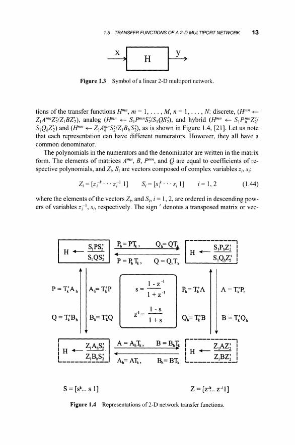
tions of the transfer functions H"", m = 1, ... , M, n = 1, ... , N: discrete, tH?" ~ZlAmnZ~/ZlBZ;), analog (Hmn ~ SlpmnS~/SlQS~), and hybrid tH?" ~ SlPhnz~/

SlQhZ;) and tH?" ~ ZlAhnS~/ZlBhS~),as is shown in Figure 1.4, [21]. Let us notethat each representation can have different numerators. However, they all have acommon denominator.

The polynomials in the numerators and the denominator are written in the matrixform. The elements of matrices Amn, B, P?", and Qare equal to coefficients ofrespective polynomials, and Z;, S; are vectors composed of complex variables Z;, s.:

Z;= [z jk . . . zi l l ] i = 1,2 (1.44)

where the elements of the vectors Z;, and S;, i = 1, 2, are ordered in descending powers of variables Z;-l, s.; respectively. The sign' denotes a transposed matrix or vee-

-----------1H +- SIPtZ; I

SIQhZl I

1 -I- Z

s=--1 + Z·I

1 - s

l+s

r-----------lB = Bh4 I ZIAZ2' I

--------.~ I H ..- -- I

~= BTkL ~I~!iJ

S = [Sk... S 1]

Figure 1.4 Representations of 2-D network transfer functions.

(1.45)


tor. Let us note that the transfer function in the discrete domain is usually written inthe form

Zl mnz'Hmn ~ ~ "", 2

ZI BZ~

where the elements of the vector Zj are ordered in ascending powers of the variable

zi1

Z. = [lz:- 1 ••• z:-k]1 1 1 (1.46)

and where jmn, Bdenotes the matrices Amn, B transposed with respect to both diagonals. The description given by (1.45) is called the standard form of a transfer function.

The vectors SI' Sb ZI' and Z2 are used for describing polynomials in the numerators and denominators of the transfer functions. It does not mean that polynomialsare of the same order with respect to the given variable because some rows orcolumns in the matrices Amn, B, I"'", and Q may be composed of zero elements. Forexample, the denominator of the transfer function of a nonrecursive filter is equal to1 in the digital domain. One can describe this filter by the matrix B in the form

oo

o r] (1.47)

We assume that the discrete and analog variables are bilinearly transformed

l- z i 1

s.>1 1 + zi1

-1 1 -SjZ: =--

1 1 + s, , i = 1,2 (1.48)

The above relationships are obtained from (1.28) and (1.29) where, for the sake ofsimplicity, we will assume that the sampling periods in both dimensions i = 1, 2 areT = 2. Under these assumptions, we can obtain all transfer function representations,multiplying matrices Amn, B, r», and Q by the transformation matrix Tk. The matrix T, can be generated in a recurrent manner:

[- 1

To = [1], T1 = 1 1] T=[-~1 ' 2 1

-2o2

1.5 TRANSFER FUNCTIONS OF A 2-D MUL TlPORT NETWORK 15

3 -3-1 -1-1 1

3 3

(1.49)

The procedure for construction of these matrices is as follows. The (i-l )th rowof the matrix 1)-1 and the ith row of the matrix 1), i = 2, ... ,} + I,} = 1, ... , k, always form two neighboring rows of a Pascal triangle with To = [1]. For example,the first row of To, the second row of T1, the third row of Tb and the fourth row ofT3, etc. form a Pascal triangle. Similarly, the first row of Tb the second of Tb thethird row of T3, etc., or the first row of T2 and the second row of T3, etc. also formPascal triangles. As far as the first row of each matrix is concerned, the lth elementof the first row of the }th matrix is the lth element of the last row of the same matrixmultiplied by (-1 )i+l+ 1•

Using the bilinear transformation we can write

(1.50)

and

(1 - z')"(1 + z-I)(1 - z-l)n-1

s (1 + z-I)(1 + z-l)n-2(1 - Z-I)

(1 + z-I)(1 + z-I)n-l

(1.51 )

The comparison of (1.50) and (1.51), for n = 1 and n = k, yields

(1.52)

where the scaling factor 1/(1 + Z-I)k, which does not affect the transfer function H"!",has been dropped. We see that both s to Z-1 and Z-1 to s transformations in (1.48)have the same form. Hence, similarly to (1.52), we can write

(1.53)

and we see that, instead of the inverse matrix T;-I, the matrix T, can be used for theinverse z to s transformation. We find that

(1.54)


where U is a unit matrix. Hence, the normalization factor of matrix T, is I/Y2k• Thetransposition of (1.52) and (1.53) gives

S=ZTi

and

Z=STi

which completes the proof of relations

Ahln = AmnTk, Amn = AJ:lnTk, B, = BTb B = BhTk

pmn = TiA;:ln, Ahln == Tipmn, Q = TiBh,B, = TiQ

Amn = TiPr:n,Pr:n == TiAmn, B = TiQh' Qh= TiB

shown in the scheme in Figure 1.4.

1.6 PROBLEMS

(1.55)

(1.56)

(1.57)

1. On the basis of (1.6) prove that the Fourier series (1.4) in the complex form isequivalent to the Fourier series in the trigonometric form:

ao cc r (21T) (21T)1x(t) = - + L ancos -nt + b, sin -nt2 n=l r, Tp

(1.58)

2. On the basis of the definition (1.10), calculate the Laplace transform X(s) ofthe function x(t) = e".

3. Calculate the Laplace transforms shown in Table 1.1 of the functions e-at, sinwaf, cos waf, e-at sin{3t, and e-atcos {3t.

Hint: Use the result from the previous example, introducing A= -a, A= jio;or A == -a + j {3.

4. Calculate the Fourier series defined by (1.4), (1.5) of the periodic function

5. Prove the relation

I 8(f-kT)k=-x

(1.59)

(1.60)

1.6 PROBLEMS 17

used in (1.21), which means that the Fourier transform of a sequence of impulses is also a sequence of impulses.

Hint: Use the inverse Fourier transform given in (1.7) and the result of theprevious problem.

6. Prove the relation (1.31).

7. Choose appropriate relations from (1.57) and calculate Hi(zb S2), H{'(s b Z2),and H2(z1, Z2) for the transfer function

[s1 1]P[s ~ S2 1]'R(s s) = -----

b 2 [SI l]Q[s~ S2 1]'(1.61)

where

P> r~oo Q=r~

oo (1.62)

Note that the 2-D transfer function (1.61) is obtained from the transfer function ofthe first-order high-pass filter:

(1.63)

after the substitution s = SI + s~.

CONTINUOUS AND DISCRETE SIGNALS

Documents

Transcript of CONTINUOUS AND DISCRETE SIGNALS