Discrete Array Representation of Continuous Space-time ...

Turk J Elec Engin, VOL.10, NO.2 2002, c© TUBITAK

Discrete Array Representation of Continuous

Space-time Source Distributions

Amir SHLIVINSKI and Ehud HEYMANDept. of Electrical Engineering - Physical Electronics,Faculty of Engineering, Tel Aviv University-ISRAEL

Abstract

We consider the realization of a continuous space-time source distributions using a sparse non-uniform

point-source array. The construction determines the largest possible cells corresponding to the local source

parameters in order to obtain a sparse array, while meeting an error criterion on the pulsed radiation

pattern. The scheme is applied for the realization of collimated short-pulse beam fields. The error criterion

is imposed within the main beam direction, while outside this region the relative realization error can be

large but it is negligible since the field there is small compared to the main beam field.

Key Words: slant stack transform, ultra-wide band short-pulse signals, continuous space-time source

distribution, sparse non-uniform point source array

1. Introduction

The increased interest in the radiation and reception of ultra-wideband short-pulse (UWB-SP) signals hasmade an impact on the design of UWB antennas and in particular on UWB-SP array antennas that arecapable of radiating and steering collimated short pulsed fields (pulsed beams). Such arrays are referred

to as “pulsed-antenna arrays,” “transient arrays” or “delay arrays” [1-7]. Most applications, for examplethose involving high resolution two- and three-dimensional imaging, require very large arrays that mustbe properly thinned to avoid an unrealistic cost, complicated electronics, and managing of huge data-flowfor real-time processing. However, array thinning based on conventional narrowband (frequency domain)considerations applied at the highest frequency in the signal spectrum leads to unnecessarily ultra-densearrays since it does not utilize the fact that the resulting wave-fields are localized in space and in time.The limitations on the array geometry in this frequency domain approach are due to phase-interference(kinematic) phenomena and are therefore irrelevant in the SP field regime. The kinematic properties of

SP arrays have been studied recently in [4, 7]. Reference [7] dwells on the transition of the kinematicphenomena from the narrowband regime to the UWB-SP regime and demonstrates in particular how thegrating lobes that characterize narrowband arrays are replaced by “cross-pulse lobes” that depend on thepulse repetition rate. This gives rise to possible sparse arrays whose inter-element spacing is much largerthan the wavelengths in the frequency band and basically does not suffer from severe side lobe problems.

A different approach is considered in the present paper which is concerned with an array realizationof continuous source distributions for collimated short-pulse beam fields. Several classes of such wave-fieldshave been introduced in the last two decades (for a review, see the Introduction in [8]). Our goal is tosynthesize such fields using an array of pulsed point sources that will reconstruct the time-dependent far

257

Turk J Elec Engin, VOL.10, NO.2, 2002

field pattern within a certain cone around the “main beam” direction and within a specified error. It isrequired that the array will have the smallest number of elements possible.

The analytically specified continuous sources are typically characterized by non-uniform space-timedistributions, hence each array-element in the discretized formulation must compensate for both the ampli-tude and the waveform variations of the idealized (i.e., continuous) distribution within the local cell. Thissets a limit on the dimensions of each one of the cells in the array as a function of the local pulse-lengthand of the transverse variation of the source-waveform. The final non-uniform array geometry (and thus

the number of its elements) is then determined by weighting the errors from the individual cells in order to

meet the total error criterion within a given space-time window; the cell dimensions (and thereby the array

sparsity) are proportional to the error level allowed.

The general conditions derived in this approach are applied for the array-realization of the so calledcomplex source pulse beam (CSPB also termed iso-diffracting pulsed beam) [8]. Compared with a con-ventional monochromatic array design, the resulting non-uniform array is shown to be ultra-sparse withinter-element spacing much larger than the wavelength of the frequencies in the band.

The paper is organized as follows. The problem is formulated in Section 2 in term of the slantstack transform (SST) of the continuous space-time source distribution [9-12]. In Section 3, the continuousdistribution is divided into cells and the contribution of each cell to the time-dependent radiation pattern isanalyzed locally. These results are compared in Section 4 with the radiation pattern of an array of pulsedpoint-sources where it is required to use the smallest number of array elements while reconstructing theradiation patterns within a certain cone around the “main beam” direction. Imposing this error constraintand maximizing the cell’s size yields expressions for the local cell’s dimensions and to the design algorithm(Section 4.3). An example of a PB array realization is presented in Section 5 followed by concluding remarksin Section 6.

2. Problem Formulation: Array Realization of Continuous Source

Distribution

We are interested in the far field u(r, t) radiated by a pulsed source distribution Q(r, t) in a uniformthree-dimensional space with wavespeed c . The field satisfies the time-dependent wave equation(

∇2 − 1c2∂2

∂t2

)u(r, t) = −Q(r, t), Q(r, t) = q(x, t)δ(z), (1)

where r = (x, z) with x = (x1, x2) being the coordinates transverse to z . It is assumed that Q(r, t) is asurface source distribution confined in the z = 0 plane within a disk of radius R0 centered at the originssuch that

q = 0 for

{|x| > R0

t ∈/

(0, T ).(2)

It is also assumed that the source generates a collimated pulsed beam field that propagates essentially alongthe z axis.

Our goal is to synthesize the field using an array of point sources that will reconstruct the far fieldpattern within a certain cone around the “main beam” direction z and up to a specified error. It is requiredthat the array will have the smallest number of elements possible.

258

SHLIVINSKI, HEYMAN: Discrete Array Representation of Continuous Space-time Source...,

The time-dependent radiation pattern of the continuous source distribution is described by the timederivative of the slant stack transform (SST) of q , defined by

q(ξ, t) =∫d2x q(x, t+ ξ · x/c), (3)

with ξ = (ξ1, ξ2). This standard operation has been introduced in [9, 10, 11, 12] in connection with the time

dependent plane wave spectrum and radiation pattern, and has also been studied extensively in [12]. Having

calculated q(ξ, t), the field in the far radiation zone is given by

u(r, t)∣∣∣r→∞

=∂tq(ξ, t− r/c)

4πr

∣∣∣ξ=br⊥

(4)

where r⊥ = r − z(r · z) = sin θ(cos φ, sinφ) is the projection of the observation direction r onto the z = 0

plane. We may therefore refer to ∂tq(ξ, t) as the time domain radiation pattern.

In the array realization, the source distribution is described by a non uniform array of point sourcesQn(t) located at points xn in the z = 0 plane where n is an index. The radiation pattern produces by this

array is given by (4) with

qarray(ξ, t) =∑n

Qn(t+ ξ · xn/c). (5)

Our goal is to determine the sparsest array such that (5) will provide a valid representation for (3) within a

given cone θ < Θ about the z -axis (see (20) and (22)), where Θ typically depends on the application. In

(18a) it will be shown to first order that Qn are given by

Qn(t) = Snq(xn, t) (6)

where Sn is the area on the cell adjacent to xn .

3. Local Evaluation of the SST

Following the discussion above, we shall quantify in this section the radiation-pattern error introduced bythe array-realization of the continuous distribution, and thus to establish criteria for the array design. Wetherefore divide the continuous distribution into a non-uniform array of cells that are centered at xn , andthen calculate q of (3) as a sum of the cell contributions. The resulting pattern will then be compared to

that of the point source array in (5) and the error criteria will be imposed in Section 4.

The SST q in (3) is given now by

q(ξ, t) =∑n

qn(ξ, t) (7)

where the SST contribution of an individual cell is

qn(ξ, t) =∫x∈ nth cell

d2x q(x, t+ ξ · x/c) (8a)

=∫|ηi|<dni

d2η q(xn + OnTη, tn + ξn · η/c). (8b)

259


1η2η2x

1x

nx

Figure 1. Single cell coordinate system

In (8b) we introduced conveniently the local coordinates η = (η1, η2) around xn

x = xn + ηOn, On =[

cosψn sinψn− sinψn cosψn

], (9)

where On is a rotation matrix at an angle ψn such that the local coordinates η coincide with the cellorientation (see Figure 1), and dn1

× dn2are cell’s dimensions. In this system tn = t + ξ · xn/c is the

reference time at the cell center and ξn = ξOnT denotes the rotated spectral coordinates, with T denoting

the transpose.

Next we derive an approximate expression for the SST contribution (8) of each cell. We first express the

space-time source distribution in the cell in a format that is amenable for the SST calculations (Section 3.1),

and then evaluate the local SST (Section 3.2).

3.1. Local model for the field in a cell

Our first step is to obtain a simplified expression for the time-dependent field in the vicinity of xn that isamenable for a closed form calculation of qn . It is convenient to start in the frequency domain where fieldconstituents are denoted by the caret and are related to the time domain constituents via

u(t) =1

2π

∫ ∞−∞

dω e−iωtu(ω). (10)

We express the initial frequency domain field in the vicinity of xn as

q(x, ω) = q(xn, ω)eiΦn(η,ω), i.e. Φn(η, ω)|η=0 = 0. (11)

Next we expand Φn in a Taylor series in ω and η near xn . We also assume that Φn is predominantlylinear in ω , i.e. it mainly describes a distributed delay. Thus, for small η

Φn(η, ω) = ωTn(η) + . . . (12a)

Tn(η) =∑i

Tniηi + 12

∑i,j

Tnijηiηj + . . . (12b)

260


with Tni = ∂ω∂ηiΦn , Tnij = ∂ω∂2ηiηjΦn , and i = 1, 2. In (12a) we neglected terms of order η, η2, . . .

that describe a frequency-independent spatial envelope, and terms of order ω2η . . . , ω3η, . . . that introducedispersive components into Φn . Thus Tn(η) represents a non-dispersive “delay” but it may be complex sothat it describes the amplitude variation near xn as will be explained next.

In order to accommodate the complex “delay” Tn(η) we utilize the analytic signal formulation.

Referring to (10), the analytic signal+u corresponding to a given real signal u(t) for t ∈ R , and with

frequency spectrum u(ω), is defined via the one-sided inverse Fourier transform

+u(τ ) =

1π

∫ ∞0

dω e−iωτ u(ω) . (13)

This integral defines an analytic function in the complex τ plane whose region of analyticity depends on the

asymptotic behavior of u : if u(ω) ∼ O(e−αω) for ω → ∞ where α > 0 is a constant then+u(τ ) is analytic

for Im τ < α .Applying (13) to (11) with (12a) yields for x ≈ xn (i.e., for small η )

q(x, t) ≈ Re+q(xn, t− Tn(η)). (14)

The real part of Tn(η) represents a pure delay (positive or negative) relative to the signal at xn , but the

imaginary part causes a change of the signal and of its magnitude. For η such that ImTn(η) ≷ 0 the signal

decays or grows relative to its value at xn , respectively. As follows from the discussion in (13), ImTn(η)

should be smaller than some positive constant (say α > 0) that is typical large for smooth q(x, t). Thus the

smoothness of q determines the range of validity of (14) about xn .

3.2. Local evaluation of the SST

Next, we insert (14) with (12b) to the SST integral (8) and expand the integrand into a Taylor series around

tn = t+ ξ · xn/c . Collecting terms of equal order in η yields

q(xn + OT

nη, tn + ξn · η/c) =∑j

jqn(η, t) (15)

where the left-hand subscripts denotes the index of the series in (15) with jqn ∼ O(ηj), and

0qn(η, t) = Re{+q(xn, tn)

}, (16a)

1qn(η, t) = Re{+q(1)(xn, tn)

∑i

(ξni/c−Tni)ηi}

(16b)

2qn(η, t) = 12 Re

{− +q(1)(xn, tn)

∑i,j

Tnijηiηj ++q(2)(xn, tn)

[∑i

(ξni/c−Tni )ηi]2} (16c)

with tn = t + ξ · xn/c (see (8)). Here ξni with i = 1, 2 denotes the ith coordinate of ξn as defined after

(9) and+q(k) ≡ ∂kt

+q . Performing the integration in (8b) within the cell, using (15) and (16), yields a series

approximation for qn

qn(ξ, t) = 0qn(ξ, t) + 2qn(ξ, t) +O(d6) , (17)

261


where jqn ∼ O(dj+2)

0qn(ξ, t) = SnRe{+q(xn, tn)

}(18a)

2qn(ξ, t) =Sn24

∑i

d2ni Re

{(ξni/c−Tni )2+

q(2)(xn, tn) − Tnii+q(1)(xn, tn)

}(18b)

with Sn = dn1dn2

is the area of the nth cell.

4. Error Analysis of the Point-Sources-Array Realization

4.1. Error criteria

From (18a), the first term in (17) represents an isotropic point source contribution, thus justifying the point

source array realization in (5)–(6). The second term represents the effects of the finite cell size and of the

linear and quadratic variations of Tn over the cell (recall that in general Tni and Tnii are complex as

discussed in connection with (14)). This second term will therefore be used to quantify the radiation-patternerror introduced by the realization of the continuous source distribution using the sparse point sourcesarray. The array geometry will then be determined by setting a given bound on the error for all observationdirections within a specific cone θ ≤ Θ about the z -axis (see discussion after (5)).

Below we shall consider separately the error en(ξ) introduced by neglecting the second term in (17)

in the individual cell contribution and then the total error of the array realization e(ξ).

The relative error introduce by describing a single cell contribution using a point source as in the firstterm in (17) (see also (6)) is given by

en(ξ) ≡ ‖qn(ξ, t)− 0qn(ξ, t)‖‖qn‖

' ‖2qn(ξ, t)‖‖0qn‖

(19)

where in the second equality we used (17). It is required that

en(ξ) ≤ ε ∀ |ξ| < sin Θ (20)

where ε is a prescribed bound.Similarly, the total error introduced by the point source realization, normalize relative to the radiation

pattern along the main beam axis is given by

e(ξ) ≡ ‖q(ξ, t)− qarray(ξ, t)‖

‖q(0, t)‖ ' ‖∑n 2qn(ξ, t)‖‖q(0, t)‖ (21)

where qarray is defined in (5). It is required that

en(ξ) ≤ ε ∀ |ξ| < sin Θ (22)

where ε is another prescribed bound. Clearly one should choose ε� ε .

4.2. Error analysis

The norm in the definitions above can be of any type: It should be chosen according to the observables (i.e.,

field-detectors) that are used to quantify the radiation pattern (e.g. L1 , L2 , or L∞ norms). In the example

of Section 5 we use the L2 (energy) norm.

262


Using (18b) and the triangle inequality for the norm in the numerator of (19) and noting also from

(18a) that ‖0qn‖ = Sn‖q(xn, t)‖ we obtain

en ≤∑i

d2ni

Eni(ξni)‖qn‖

(23)

with

Eni(ξni) ≤124{|ξni/c− Tni |2‖q(2)

n ‖ + |Tnii|‖q(1)n ‖}

(24)

where ‖qn‖ ≡ ‖q(xn, t)‖ , ‖q(1)n ‖ = ‖∂tq(xn, t)‖ , etc. In the derivation, the norms of the analytic signals in

(18) were evaluated on the real argument axis where for the L2 norm we have ‖+q‖ =

√2‖q‖ .

Maximizing the cell size Sn = dn1dn2

subject to the error constraint in (20) yields the cell dimensions

dni(xn) = min|ξ|<sin Θ

[ε

2‖qn‖

Eni(ξni)

] 12

, i = 1, 2 (25)

From (24), the largest Eni in the range |ξ| < sin Θ is obtained for |ξ| = sin Θ. Maximization on the

azimuthal spectral angle ψn is problem dependent, hence we shall use a typical value: ξn = (ξn1, ξn2

) '( 1√

2, 1√

2) sin Θ. The result in (25) yield the largest cell that can be described by a point source, as a function

of the local source properties.

Next we shall consider the constraint (22) on the total radiation pattern error. Eq. (21) defines thetotal error as a sum of the single cell errors and hence it does not relate directly to the single cell dimensions.We therefore rearranging (21) as

e(ξ) '∥∥∥∑n en(ξ)2qn

‖2qn‖

∥∥∥ ≤ ε (26a)

where

en(ξ) ≡ ‖2qn(ξ, t)‖‖q(0, t)‖ ≤ Sn

∑i

d2ni

Eni(ξni)‖q(0, t)‖ (26b)

is the single element error normalized to q(0, t), and the last inequality follows from (18b) with (24). It willbe required that

en(ξ) ≤ ε ∀ |ξ| < sin Θ and ∀n (27)

where ε is a parameter to be determined. To find a bound on ε we use norm inequality to e(ξ) obtaining

e(ξ) ≤ ε∥∥∥∑n 2qn/‖2qn‖

∥∥∥ . Next we recall that the error criterion should be imposed outside the main beam

direction (for ξ ≈/ 0). Noting that in this region the delayed-error terms 2qn are not coherent it follows that∥∥∥∑n 2qn/‖2qn‖∥∥∥ ∼ O(1), suggesting that in this range ε ∼ ε . Using this value of ε in (27) together with the

last term on the right hand side of (26b) and maximizing the cell area as in (25) yields

dni(xn) = min|ξ|<sin Θ

[( ε2‖q(0, t)‖

)1/4[En1

(ξn1)En2

(ξn2)]1/8

[Eni(ξni)]1/2

](28)

where as noted after (25) may shall use a typical value ξn ' ( 1√2, 1√

2) sin Θ.

263


4.3. Array design considerations

Equation (25) and (28) provides two constraints on the cell size dni , i = 1, 2 and for all n . The values of dniobtained from (25) sets an upper limit on the cell size for which the second order analysis is valid, whereas

those obtained via (28) are concerned only with meeting the constraint on the total radiation pattern. For

focusing apertures, q(x, t) is typically large near the center hence the condition (28) dominates for this

elements. Consequently, the dimensions of the central cells are found from (28) yielding a rather dense

array. Far from the center q weakens and the cell dimensions implied by (28) grow until they disagree with

the condition in (25) which then becomes operative. The array construction starts therefore from the center

and proceeds outward where at each step one calculates dn1,2(xn) via the condition in (25) or (28).

When the procedure above is applied to scanning arrays, the array sparsity is determined by the mostrestrictive constraints corresponding to all the possible scan directions within a given range. Consider thecase where the array should stir a given collimated pulsed beam (PB) for all directions within a cone ofangle θmax about the z axis. The analysis for each direction proceeds essentially as discussed above, butby considering all possible scan directions one finds that the resulting array geometry is almost the sameas obtained for a fixed broadside array that radiates a PB along the z -axis. In fact, the size of the arrayshould be increased by a factor 1/ cos θmax , so as to obtain the same effective aperture at the largest scanangle, but the interelement spacing should remain essentially the same so as to accommodate all the scandirections within the cone.

To be more specific, for a scan in the direction (θ0, φ0), the complex delay T (η) (see Section 3.1) is

augmented by a linear delay T (x) = c−1[x1 sin θ0 cosφ0 + x2 sin θ0 sinφ0] . For simplicity let the local cellgeometry be oriented such that η1 coincides with the scan direction. Consequently, each one of the the

parameters Tn1of (12b) is augmented by c−1 sin θ0 . It then follows from (24) that En1

is minimized for

observations along the beam axis where ξn1= sin θ0 . Substituting En1

in Eqs. (25) and (28) and considering

observation directions within a cone Θ about the PB direction (θ0, φ0 = 0), one obtains essentially the samerealization constraints as obtained for radiation along the z -axis. Finally, these considerations should berepeated for all scanning directions within the θmax cone. For this reasons the example of Section 5 belowconsiders only the realization for a broadside radiating array.

5. Example: Iso-Diffracting Source Distribution

We consider a circular symmetry pulsed aperture distribution of the form

q(x, t) = Re+

f [t− i|x|2/2bc], (29)

where+

f(t) can be any analytic signal and b is a positive parameter. In [10] this distribution has beentermed “iso-diffracting” since all its frequency components have the same collimation distance b . Indeed,looking at its frequency spectrum for ω > 0,

q(x, ω) = f(ω) exp{−ω|x|2/2bc} (30)

where f(ω) is the spectrum of+

f(t), one finds that the width of the Gaussian x-distribution varies with ω

like√bc/ω , hence its Rayleigh (collimation) distance is given by b for all ω .

264


In the examples below we choose+

f to be the n-times differentiated analytic-δ signal

+

f(t) =+

δ(n)(t− iT0/2) = Re{ (−)nn!πi(t − iT0/2)n+1

}(31)

where T0>0 is a parameter that defines the pulse length. To understand the properties of (29) we use n = 2

in (31) and write (29) explicitly for this case, obtaining

q(x, t) = Re+

δ(2)(t− iγ/2) =γ

π

[3t2 − (γ/2)2

][t2 + (γ/2)2 ]3

(32)

where γ = T0 + |x|2/bc . Analyzing the waveform in (32) one observes that the pulse length is given by γ and

hence it grows with |x| . In addition, the waveform decays as γ grows, hence the half-amplitude diameter

that describes the decay in |x| is found to be W0 = 1.02√cT0b . Plots of q(x, t) at x = 0, 1

2W0, W0 and

2W0 are given in Figure 7b.Considering next the radiation properties of this source one finds that if the parameters are chosen

such that cT0/b � 1 then (29) generates a collimated pulsed beam (PB) field that propagates along the

z -axis, having collimation length b and beamwidth W (z) = W0

√1 + z2/b2 so that for z � b it expands

along a constant diffraction angle Θ0 = 0.64√cT0/b� 1. (see e.g., [10], for a thorough review of PB fields

see [8]).

In the examples below we choose n = 2 and cT0/b = 0.001. We design the point source array to

realized the radiation pattern of the continuous distribution (29) subject to the error constraints ε = 0.01

and ε = 0.5 (see (19)–(22)) within the cone whose angle Θ equals to the PB diffraction angle Θ0 . We shallcompare the resulting array with an array designed to meet the error criteria within a wider cone θ ≤ 3Θ0 .

The arrays have been designed using (25), (28) and the design considerations of Section 4.3. The

cells have been rotated so that (η1, η2) coincide with the radial and azimuthal coordinates, respectively.

Comparing (14) with (29), the parameters in (25) and (28) are Tn1 = iρn/bc , Tn2 = 0 and Tn11 = i/bc = Tn22

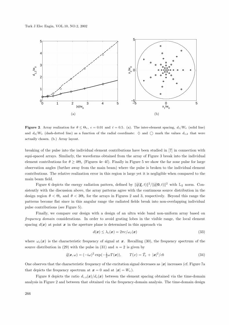
with ρn = |xn| .Figure 2a depicts the inter element spacing dn1,2

(solid and dashed lines for the radial and azimuthal

dimensions, respectively) as a function of the radial coordinate for the realization with Θ = Θ0 . Alldimensions are normalized to W0 . The values dn1,2

that were actually chosen to minimize the number of

elements are denoted by ♦ and © . For |x| < 1.3W0 , dn1,2are relatively small and are determined by (28).

For |x| > 1.3W0 , the values obtained from (28) are larger than those obtained via (25) hence dn1,2were

calculated there via (25). Figure 2b depicts the array layout: the array is denser at the center and consistsof a total of 44 elements within a circle of radius 4.7W0 .

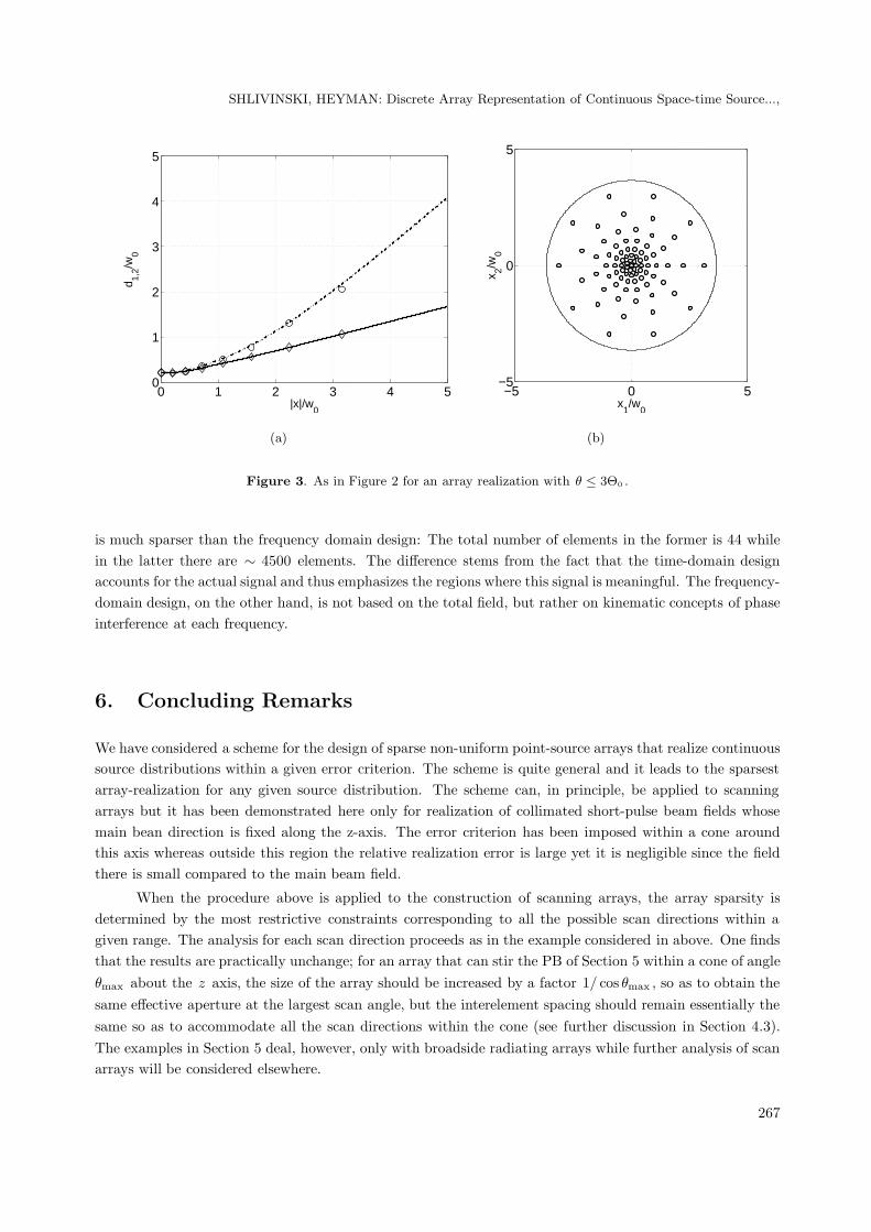
Figure 3 depicts the results for an array designed to meet the same error criteria within a wider coneΘ = 3Θ0 . The array dimensions were determined via (28) and (25) for |x| ≶ 0.87W0 , respectively, giving atotal number of 82 elements within a supporting radius 3.7W0 .

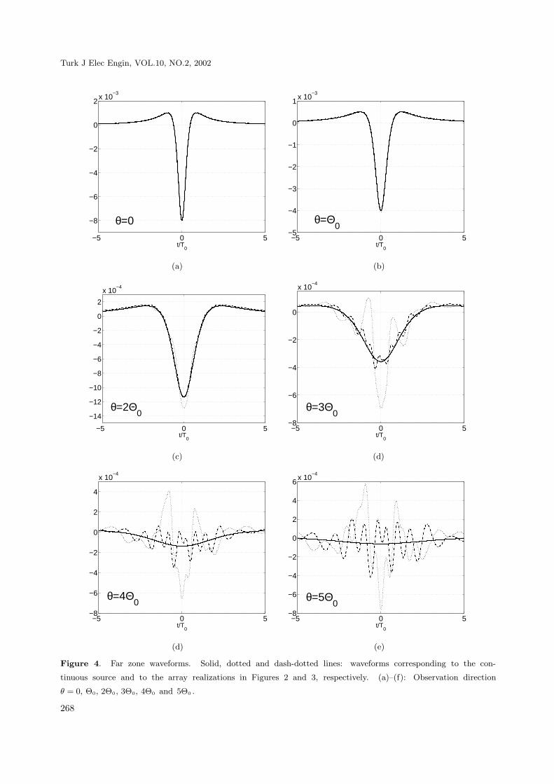
Figure 4 depicts the far-zone pulse at several observation angles: The solid, the dotted and the dash-dotted lines correspond, respectively, to the continuous distribution and to the array realizations of Figures 2and 3. One observes an excellent agreement for θ = 0 and θ = Θ0 (Figures 4a and 4b). For θ ≥ 2Θ0 , i.e.,beyond the design range of the array of Figure 2, the waveforms corresponding to that array break into theindividual element contributionss (Figures 4c–4d; note the different scales in the figures). The conditions for

265


0 1 2 3 4 50

1

2

3

4

5

|x|/w0

d 1,2/w

0

−5 0 5−5

0

5

x1/w

0

x 2/w0

(a) (b)

Figure 2. Array realization for θ ≤ Θ0 , ε = 0.01 and ε = 0.5. (a). The inter-element spacing, d1/W0 (solid line)

and d2/W0 (dash-dotted line) as a function of the radial coordinate: ♦ and © mark the values d1,2 that were

actually chosen. (b.) Array layout.

breaking of the pulse into the individual element contributions have been studied in [7] in connection withequi-spaced arrays. Similarly, the waveforms obtained from the array of Figure 3 break into the individualelement contributions for θ ≥ 4Θ0 (Figures 4e–4f). Finally in Figure 5 we show the far zone pulse for large

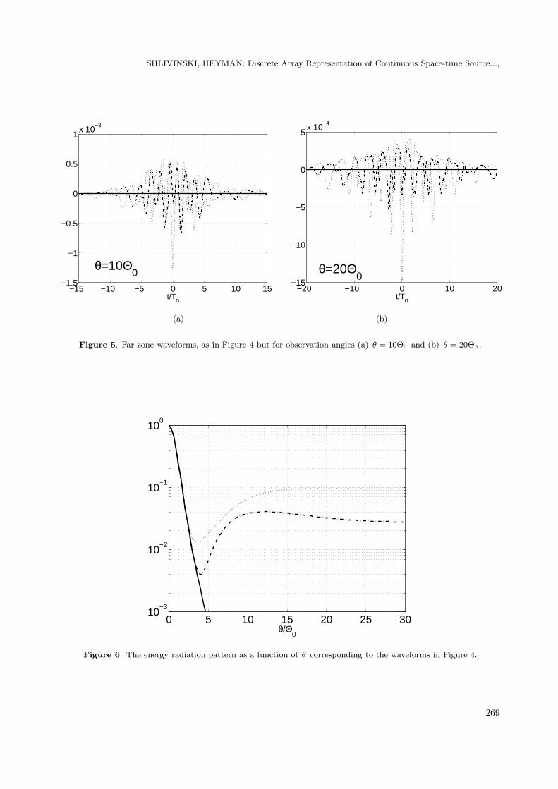
observation angles (further away from the main beam) where the pulse is broken to the individual elementcontributions. The relative realization error in this region is large yet it is negligible when compared to themain beam field.

Figure 6 depicts the energy radiation pattern, defined by ‖q(ξ, t)‖2/‖q(0, t)‖2 with L2 norm. Con-sistently with the discussion above, the array patterns agree with the continuous source distribution in thedesign region θ < Θ0 and θ < 3Θ0 for the arrays in Figures 2 and 3, respectively. Beyond this range thepatterns become flat since in this angular range the radiated fields break into non-overlapping individualpulse contributions (see Figure 5).

Finally, we compare our design with a design of an ultra wide band non-uniform array based onfrequency domain considerations. In order to avoid grating lobes in the visible range, the local elementspacing d(x) at point x in the aperture plane is determined in this approach via

d(x) ≤ λc(x) = 2πc/ωc(x) (33)

where ωc(x) is the characteristic frequency of signal at x . Recalling (30), the frequency spectrum of the

source distribution in (29) with the pulse in (31) and n = 2 is given by

q(x, ω) = (−iω)2 exp(−12ωT (x)), T (x) = T0 + |x|2/cb (34)

One observes that the characteristic frequency of the excitation signal decreases as |x| increases (cf. Figure 7a

that depicts the frequency spectrum at x = 0 and at |x| = W0 ).

Figure 8 depicts the ratio d1,2(x)/dc(x) between the element spacing obtained via the time-domainanalysis in Figure 2 and between that obtained via the frequency-domain analysis. The time-domain design

266


0 1 2 3 4 50

1

2

3

4

5

|x|/w0

d 1,2/w

0

−5 0 5−5

0

5

x1/w

0

x 2/w0

(a) (b)

Figure 3. As in Figure 2 for an array realization with θ ≤ 3Θ0 .

is much sparser than the frequency domain design: The total number of elements in the former is 44 whilein the latter there are ∼ 4500 elements. The difference stems from the fact that the time-domain designaccounts for the actual signal and thus emphasizes the regions where this signal is meaningful. The frequency-domain design, on the other hand, is not based on the total field, but rather on kinematic concepts of phaseinterference at each frequency.

6. Concluding Remarks

We have considered a scheme for the design of sparse non-uniform point-source arrays that realize continuoussource distributions within a given error criterion. The scheme is quite general and it leads to the sparsestarray-realization for any given source distribution. The scheme can, in principle, be applied to scanningarrays but it has been demonstrated here only for realization of collimated short-pulse beam fields whosemain bean direction is fixed along the z-axis. The error criterion has been imposed within a cone aroundthis axis whereas outside this region the relative realization error is large yet it is negligible since the fieldthere is small compared to the main beam field.

When the procedure above is applied to the construction of scanning arrays, the array sparsity isdetermined by the most restrictive constraints corresponding to all the possible scan directions within agiven range. The analysis for each scan direction proceeds as in the example considered in above. One findsthat the results are practically unchange; for an array that can stir the PB of Section 5 within a cone of angleθmax about the z axis, the size of the array should be increased by a factor 1/ cos θmax , so as to obtain thesame effective aperture at the largest scan angle, but the interelement spacing should remain essentially thesame so as to accommodate all the scan directions within the cone (see further discussion in Section 4.3).The examples in Section 5 deal, however, only with broadside radiating arrays while further analysis of scanarrays will be considered elsewhere.

267


−5 0 5

−8

−6

−4

−2

0

2x 10

−3

t/T0

θ=0−5 0 5

−5

−4

−3

−2

−1

0

1x 10

−3

t/T0

θ=Θ0

(a) (b)

−5 0 5

−14

−12

−10

−8

−6

−4

−2

0

2

x 10−4

t/T0

θ=2Θ0

−5 0 5−8

−6

−4

−2

0

x 10−4

t/T0

θ=3Θ0

(c) (d)

−5 0 5−8

−6

−4

−2

0

2

4

x 10−4

t/T0

θ=4Θ0

−5 0 5−8

−6

−4

−2

0

2

4

6x 10

−4

t/T0

θ=5Θ0

(d) (e)

Figure 4. Far zone waveforms. Solid, dotted and dash-dotted lines: waveforms corresponding to the con-

tinuous source and to the array realizations in Figures 2 and 3, respectively. (a)–(f): Observation direction

θ = 0, Θ0, 2Θ0, 3Θ0, 4Θ0 and 5Θ0 .

268


−15 −10 −5 0 5 10 15−1.5

−1

−0.5

0

0.5

1x 10

−3

t/T0

θ=10Θ0

−20 −10 0 10 20−15

−10

−5

0

5x 10

−4

t/T0

θ=20Θ0

(a) (b)

Figure 5. Far zone waveforms, as in Figure 4 but for observation angles (a) θ = 10Θ0 and (b) θ = 20Θ0 .

0 5 10 15 20 25 3010

−3

10−2

10−1

100

θ/Θ0

Figure 6. The energy radiation pattern as a function of θ corresponding to the waveforms in Figure 4.

269


0 5 10 150

0.2

0.4

0.6

0.8

1

ω T0

|x|=0

|x|=W0

ωc(x=0)

ωc(x=W

0)

−3 −2 −1 0 1 2 3−1

−0.5

0

0.5

t/T0

|x|=0

|x|=W0

|x|=0.5W0

|x|=2W0

(a) (b)

Figure 7. Source distribution q(x, t) of (29) with n = 2 at |x| = 0 and at |x| = W0 (solid and dashed lines,

respectively). (a) Frequency spectrum bq(x, ω) . (b) q(x, t) .

0 1 2 3 4 50

5

10

15

20

|x|/w0

d 1,2/λ

c

Figure 8. The ratio between the inter-element spacing d1,2(x) calculated via the time domain analysis and dc(x)

calculated via the frequency domain criterion. d1/dc - solid line. d2/dc - dash-dotted line.

270


Acknowledgement

This work has been supported in part by the Israel Science Foundation under Grant No. 404/98, and inpart by AFOSR Grant No. F49620-01-C-0018.

References

[1] F. Anderson, W. Christensen, F. Fullerton and B. Kortegaard, “Ultra-wideband beamforming in sparse arrays,”

IEE Proceedings–H, Vol. 138, pp. 342–346, August 1991.

[2] C. E. Baum, “Transient arrays,” in Proceedings of the Ultra-Wideband, Short-pulse Electromagnetics 3, C. E.

Baum et. al (eds), 129–138, 1997, Plenum Press, NY.

[3] P. Crombie P, P. A. J. Bascom and R. S. C Cobbold,“Calculating the pulsed response of linear arrays: Accuracy

versus computational efficiency,” IEEE Trans. Ultrasonic ferroelectric and frequency control, UFFC-44, 997–

1009, 1997.

[4] J.L. Schwartz and B. D. Steinberg, “Ultrasparse, ultrawideband arrays,” IEEE Trans. Ultrasonic ferroelectric

and frequency control, UFFC-45, 376–393, 1998.

[5] D.T. McGrath and C.E. Baum, “Scanning and impedance properties of TEM horn arrays for transient radiation,”

IEEE Trans. Antennas Propagat., AP-47, 469–473, 1999.

[6] B. Piwakowski and K. Sbai,“A new approach to calculate the field radiated from arbitrarily structured transducer

arrays ,” IEEE Trans. Ultrasonic ferroelectric and frequency control, UFFC-46, 422–440, 1999.

[7] A. Shlivinski and E. Heyman, “A unified kinematic theory of transient arrays,” in Proceedings of the Ultra-

Wideband, Short-pulse Electromagnetics 5, P.D Smith ed., June 2000, to be published by Plenum Press, NY.

[8] E. Heyman and L.B. Felsen, “Gaussian beam and pulsed beam dynamics: Complex source and spectrum

formulations within and beyond paraxial asymptotics,” J. Opt. Soc. Am. A, Vol. 18, pp. 1588–1611, July 2001.

[9] B.Z. Steinberg, E. Heyman and L.B. Felsen,“Phase space beam summation for time dependent radiation from

large apertures: Continuous parametrization,” J. Opt. Soc. Am. A, 8, 943–958, 1991.

[10] E. Heyman and T. Melamed, “Certain consideration in aperture synthesis for ultra-wideband/short-pulsed

fields,” IEEE Trans. Antennas Propagat., AP-42, 518–525, 1994.

[11] T. B. Hansen and A. D. Yaghjian, Plane-Wave Theory of Time-Domain Fields: Near-Field Scanning Applica-

tions, IEEE Press Series on Electromagnetic Wave Theory, New York (1999).

[12] E. Heyman, “Time-dependent plane-wave spectrum representation for radiation from volume source distribu-

tions,” J. Math. Phys., 37, 658–681, 1996.

271

Discrete Array Representation of Continuous Space-time ...

Documents

Transcript of Discrete Array Representation of Continuous Space-time ...