Convergence of discrete period matrices and discreteholomorphic integrals for ramified coverings of the

Riemann sphere

Alexander I. Bobenko and Ulrike Bücking

September 14, 2018

Abstract

We consider the class of compact Riemann surfaces which are ramified coverings of theRiemann sphere C. Based on a triangulation of this covering of the sphere S2 ∼= C and itsstereographic projection, we define discrete (multi-valued) harmonic and holomorphic functions.We prove that the corresponding discrete periodmatrices converge to their continuous counterparts.In order to achieve an error estimate, which is linear in the maximal edge length of the triangles,we suitably adapt the triangulations in a neighborhood of every branch point. Finally, we alsoprove a convergence result for discrete holomorphic integrals for our adapted triangulations of theramified covering.

1 IntroductionSmooth holomorphic functions can be characterized in different ways. In particular, the real andimaginary part of any holomorphic function is harmonic and both are related by the Cauchy-Riemannequations. This perspective naturally led to linear discretizations of harmonic and holomorphicfunctions, starting with results for square grids, see [CFL28, Isa41, Duf53]. Lelong-Ferand furtherdeveloped this theory of discrete harmonic and holomorphic functions in [Fer44, LF55]. MacNealand Duffin generalized these notions in [Mac49, Duf56, Duf59, Duf68]. In particular, they consideredarbitrary triangulations in the plane and discovered the cotan-weights. The cotan-Laplacian is alsoconsidered for triangle meshes, for example for surfaces in discrete differential geometry, see [PP93],or for applications in computer graphics, see for example [MDSB03]. Further properties and theoremsof the smooth theory of holomorphic functions have found recently discrete analogues in the discretelinear theory in [BG16, BG17].

Note that there are other important nonlinear discretizations of holomorphic functions, for ex-ample involving circle packings or circle patterns [Ste05, Sch97, BS04, Büc08], connected to cross-ratios [BP96, Mat05], using discrete conformal equivalence [BPS15, Büc16], or based on bi-coloredtriangles [DN03, Nov11]. The linear theory of holomorphic functions on rhombic lattices can beobtained as infinitesimal deformation of circle patterns [BMS05].

Mercat generalized in [Mer01] the discrete linear theory from planar subsets to discrete Riemannsurfaces and introduced in [Mer02, Mer07] discrete period matrices. In [BMS11] numerical ex-periments are considered to compute discrete period matrices for polyhedral surfaces explicitly andcompare them to known period matrices for the corresponding smooth surfaces. A convergence prooffor the class of polyhedral surfaces was obtained in [BS16].

The interest in numerical computation of period matrices is for example motivated by the com-putation of finite-genus solutions of integrable differential equations. As Riemann surfaces may be

1

arX

iv:1

809.

0484

7v1

[m

ath.

CV

] 1

3 Se

p 20

18

represented as algebraic curves, this is often taken as a starting point for computing discrete periodmatrices. Recent results in this context include [GSST98, DvH01, FK15, FK17, MN17].

In this article, we take a different approach and consider Riemann surfaces which are ramifiedcoverings of the Riemann sphere C. Based on a triangulation of this covering of the sphere S2 ∼= Cor its stereographic projection, discrete period matrices can be obtained from this discrete data.Furthermore, we prove convergence of the discrete period matrices to their continuous counterparts(Theorem 2.5). In particular, we obtain an error estimate, which is linear in the maximal edge lengthof the triangles if we adapt the triangulations in a neighborhood of every branch point. The details ofour ‘adapted triangulations’ will be explained in Section 2.3.

The convergence of discrete analytic functions to their continuous counterparts remains an im-portant issue, although several results have been proved by now. In particular, for the linear theory,convergence was first shown for the square lattice [CFL28, LF55] and recently for more general quadri-lateral lattices [CS11, Sko13, BS16]. In this article, we prove the convergence of discrete holomorphicintegrals (Abelian integrals of first kind) obtained from suitable triangulations of the ramified coveringto their continuous counterparts (Theorem 2.6).

Our main results are stated in Section 2 and proved in Section 3. The proof is inspired by [BS16]and uses energy estimates which allow to prove the convergence of the discrete periodmatrices directly.Our results are also applied to improve the convergence results of [BS16] in Section 5. Finally, inSection 6, we present some numerical experiments.

2 Convergence results for discrete period matrices and discreteholomorphic integrals for ramified coverings of C

In the following, we consider any compact Riemann surfaceR of genus g ≥ 1which allows a branchedcoveringmap f : R → C. Using this coveringmap as a local chart, we always locally identify points inR with their images in C. Then for points in C \ ∞ we apply the standard stereographic projectionto the complex plane C. This map from R to C is denoted by PrR and gives a local chart in aneighborhood about every point, except at branch points. For further use, we fix a radius % > 1 suchthat the images of all branch points, except possibly∞, have a distance at most %/2 from the origin.

Let T = TR be a triangulation ofR such that all branch points are vertices. We assume that everytriangle is contained in only one sheet of the covering. We will mostly consider this triangulationvia its (local) image under the chart PrR. In this sense, without further mention, we always identifythis triangulation with the corresponding (multi-sheeted) triangulation on C (which is the image f(T )under the covering map) and with the (multi-sheeted) image of this triangulation of C under the mapPrR, excluding the vertex at infinity. We assume that this triangulation is a locally planar embeddingin the complex plane C or equivalently in the Riemann sphere C, except at the branch points andpossibly at∞. From now on, we consider the vertices of the triangulation as points of C, except∞,that is, we always apply PrR, i.e. the covering map and the standard stereographic projection. Theedges connecting incident vertices will be straight line segments or circular arcs in C, depending onthe following distinction.

(i) All triangles with at least two vertices in the open disk B%(0) of radius % about the origin aregeodesic, that is Euclidean triangles. We always consider these triangles to be embedded in C.

(ii) All triangles whose vertices are all contained in the complement C \ B%(0) are preimages ofa geodesic triangulation with Euclidean triangles under the map z 7→ 1/z. Therefore, thesetriangles are in general bounded by circular arcs.Note that we mostly consider the images of these triangles under the map z 7→ 1/z which areEuclidean triangles embedded into C in a neighborhood of the origin.

2

te

he

le reαe

βe

Figure 1: Notation associated with an edge e = [te, he] ∈ E and with its oriented version ~e =−−→tehe.

(iii) The remaining triangles in the ’boundary region’ are consequently in general bounded by twostraight lines and one circular arc. These triangles will be called boundary triangles and denotedby F%. Finally, we assume that the edge lengths of all boundary triangles are strictly smaller thanmax%/2, 1. As in the first case, we always consider these triangles to be embedded in C.

We denote by V,E, ~E, F the sets of vertices, edges, oriented edges, and faces of TR, respectively,and identify them locally with their images under the map PrR.

2.1 Discrete harmonic functionsWe define weights on the edges E of the triangulation TR essentially by using cotan-weights, but wedistinguish three cases for edges e = [x, y] ∈ E corresponding to the different cases above:

(i) If both triangles incident to e are contained in the open disk B%(0), we use cotan-weights

c(e) =1

2cotαe +

1

2cot βe, (1)

where αe and βe are the angles opposite to the edge e ∈ E in the two adjacent triangles, seeFigure 1.

(ii) If both triangles incident to e are contained in C\B%(0), we consider the image of the triangulationunder the map z 7→ 1/z. We define the edge weights by (1) for the image triangles. Note thatthis amounts to using in (1) the angles opposite to the edge e ∈ E in the two adjacent circulararc triangles.

(iii) If e = [x, y] is incident to a boundary triangle in F%, we define the weight similarly as above as asum c(e) = C1 +C2 of two parts corresponding to the two incident triangles ∆1,∆2. If there isa non-boundary triangle, say ∆1, incident to e, we consider the angle αe in this triangle oppositeto e and set C1 = 1

2cotαe. The second part C2 = C[x,y] is defined below in (4) using a suitable

interpolation function and the smooth Dirichlet energy. More details and explicit calculationsare given in Appendix A.1.

Using our edge weights, we can define discrete harmonicity and a discrete Dirichlet energy forfunctions u : V → R on the vertices of the triangulation TR. In particular, u is called discreteharmonic if for every vertex x ∈ V there holds∑

y∈V :[x,y]∈Ec([x, y])(u(y)− u(x)) = 0. (2)

The energy of u isET (u) =

∑e=[x,y]∈E

c([x, y])(u(y)− u(x))2. (3)

3

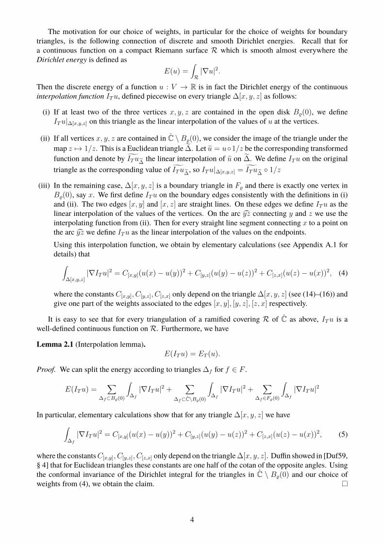
The motivation for our choice of weights, in particular for the choice of weights for boundarytriangles, is the following connection of discrete and smooth Dirichlet energies. Recall that fora continuous function on a compact Riemann surface R which is smooth almost everywhere theDirichlet energy is defined as

E(u) =∫R|∇u|2.

Then the discrete energy of a function u : V → R is in fact the Dirichlet energy of the continuousinterpolation function ITu, defined piecewise on every triangle ∆[x, y, z] as follows:

(i) If at least two of the three vertices x, y, z are contained in the open disk B%(0), we defineITu|∆[x,y,z] on this triangle as the linear interpolation of the values of u at the vertices.

(ii) If all vertices x, y, z are contained in C \B%(0), we consider the image of the triangle under themap z 7→ 1/z. This is a Euclidean triangle ‹∆. Let u = u1/z be the corresponding transformedfunction and denote by fiITu∆

the linear interpolation of u on ‹∆. We define ITu on the originaltriangle as the corresponding value offiITu∆

, so ITu|∆[x,y,z] = fiITu∆ 1/z

(iii) In the remaining case, ∆[x, y, z] is a boundary triangle in F% and there is exactly one vertex inB%(0), say x. We first define ITu on the boundary edges consistently with the definitions in (i)and (ii). The two edges [x, y] and [x, z] are straight lines. On these edges we define ITu as thelinear interpolation of the values of the vertices. On the arc ıyz connecting y and z we use theinterpolating function from (ii). Then for every straight line segment connecting x to a point onthe arc ıyz we define ITu as the linear interpolation of the values on the endpoints.Using this interpolation function, we obtain by elementary calculations (see Appendix A.1 fordetails) that∫

∆[x,y,z]|∇ITu|2 = C[x,y](u(x)− u(y))2 + C[y,z](u(y)− u(z))2 + C[z,x](u(z)− u(x))2, (4)

where the constants C[x,y], C[y,z], C[z,x] only depend on the triangle ∆[x, y, z] (see (14)–(16)) andgive one part of the weights associated to the edges [x, y], [y, z], [z, x] respectively.

It is easy to see that for every triangulation of a ramified covering R of C as above, ITu is awell-defined continuous function onR. Furthermore, we have

Lemma 2.1 (Interpolation lemma).E(ITu) = ET (u).

Proof. We can split the energy according to triangles ∆f for f ∈ F .

E(ITu) =∑

∆f⊂B%(0)

∫∆f

|∇ITu|2 +∑

∆f⊂C\B%(0)

∫∆f

|∇ITu|2 +∑

∆f∈F%(0)

∫∆f

|∇ITu|2

In particular, elementary calculations show that for any triangle ∆[x, y, z] we have∫∆f

|∇ITu|2 = C[x,y](u(x)− u(y))2 + C[y,z](u(y)− u(z))2 + C[z,x](u(z)− u(x))2, (5)

where the constantsC[x,y], C[y,z], C[z,x] only depend on the triangle∆[x, y, z]. Duffin showed in [Duf59,§ 4] that for Euclidean triangles these constants are one half of the cotan of the opposite angles. Usingthe conformal invariance of the Dirichlet integral for the triangles in C \ B%(0) and our choice ofweights from (4), we obtain the claim.

4

Remark 2.2. It will be important to note that the constants C[x,y], C[y,z], C[z,x] defined by (4) are onlysmall perturbations of the usual cotan-weights in the following sense. If the maximal edge length hin the boundary triangle ∆[x, y, z] ∈ F% is small enough and the angles in ∆[x, y, z] as well as theangles in the Euclidean triangle formed by the vertices x, y, z lie in [δ, π − δ] for some δ > 0, thenelementary calculations and estimates show that

12

cot αe − Cδ,% · h ≤ Ce ≤ 12

cot αe + Cδ,% · h.

for some constantCδ,% > 0, where αe denotes the angle opposite to the edge e in the Euclidean triangleformed by the vertices x, y, z. The details are given in Appendix A.1.

Note that the difference between the the angles in the Euclidean triangle with vertices x, y, z andthe corresponding angles in ∆[x, y, z] is of order h. Thus, for h small enough, the correspondingestimates on |Ce − 1

2cotαe| also hold for the actual angles αe in the triangle ∆[x, y, z].

2.2 Discrete analytic functions, discrete holomorphic integrals and discreteperiod matrices

In the following, we define discrete analytic functions and discrete holomorphic integrals analogouslyas in [BS16].

For an oriented edge ~e ∈ ~E, we denote by he ∈ V and te ∈ V the head and the tail of ~e, and byle ∈ F and re ∈ F the left shore and the right shore of ~e, respectively, see Figure 1. Two functionsu : V → R and v : F → R are conjugate, if for each oriented edge ~e ∈ ~E we have

v(le)− v(re) = c(e)(u(he)− u(te)). (6)

The pair f = (u : V → R, v : F → R) of two conjugate functions is called a discrete analyticfunction. We write Ref := u and Imf := v. If both u and v are constant functions, not necessarilyequal to each other, we write f = const. A direct checking shows that on simply connected surfacesdiscrete harmonic functions are precisely real parts of discrete analytic functions. Note that fornon-zero weights c(e) 6= 0 we define the (discrete) energy of a function v : F → R by

ET (v) :=∑

e=[x,y]∈E

1

c([x, y])(v(y)− v(x))2. (7)

We will consider multi-valued functions on the vertices and the faces of the triangulation T .Informally, a multi-values function changes its values after performing some nontrivial loop on thesurface.

Recall that the Riemann surface R is a branched covering of C with genus g ≥ 1. Denote byp : R → R the universal covering of R and by p : ‹T → T the induced universal covering of T . Fixa base point z0 ∈ R and closed paths α1, . . . , αg, β, . . . , βg : [0, 1] → R forming a standard basisof the fundamental group π1(R, p(z0)) such that α1β1α

−11 β−1

1 · · ·αgβgα−1g β−1

g is null-homotopic.Each closed path γ : [0, 1] → R with γ(0) = γ(1) = p(z0) determines the deck transformationdγ : R → R, that is, the homeomorphism such that p dγ = p and dγ(z0) = γ(1), where γ : R → Ris the lift of γ : [0, 1]→ S such that γ(0) = z0. The induced deck transformation of ‹T is also denotedby dγ : ‹T → ‹T .

Amulti-valued function with periodsA1, . . . , Ag, B1, . . . , Bg ∈ C is a pair of functions f = (Ref :‹V → R, Imf : ‹F → R) such that for each k = 1, . . . , g an each z ∈ ‹V , w ∈ ‹F we have

Ref(dαk(z))− Ref(z) = Re(Ak), Ref(dβk(z))− Ref(z) = Re(Bk),

Imf(dαk(z))− Imf(z) = Im(Ak), Imf(dβk(z))− Imf(z) = Im(Bk).

The numbers A1, . . . , Ag and B1, . . . , Bg are called the A-periods and the B-periods of the multi-valued function f , respectively. Analogously, we can also define multi-valued functions u : ‹V → R,

5

v : ‹F → R or u : R → R. Note in particular, that for each multi-valued function u : ‹V → Rand every edge [x, y] ∈ E the difference u(x) − u(y) is well defined. The (discrete) energy of themulti-valued function is

ET (u) =∑

[x,y]∈Ec([x, y])(u(x)− u(y))2.

Similarly, for each multi-valued function u : R → R, which is smooth on every face of ‹F , at eachpoint inside a face ∆ ∈ F the gradient∇u is well defined. The (Dirichlet) energy of the multi-valuedfunction is

E(u) =∑

∆f∈F

∫∆f

|∇u|2.

A multi-valued discrete analytic function is called a discrete holomorphic integral or discreteAbelian integral of the first kind.

Theorem 2.3 ([BS16, Theorem 2.3]). For any numbers A1, . . . , Ag ∈ C there exists a discreteholomorphic integral with A-periods A1, . . . , Ag. It is unique up to a constant.

For each l = 1, . . . , g denote by φlT = (ReφlT : ‹V → R, ImφlT : ‹F → R) the unique (up toconstant) discrete holomorphic integral with A-periods given by Ak = δkl, where k = 1, . . . , g. Theg × g-matrix ΠT whose l-th column is formed by the B-periods of φlT , where l = 1, . . . , g, is calledthe period matrix of the triangulation T .

2.3 Convergence of energy and discrete period matricesSo far, we have defined our notions like discrete energy for a rather general class of triangulations.In view of our convergence results, we now make some additional assumptions. In orde to measuredistances and other metric properties, we always consider the images of the triangles in C under theprojection PrR. By our assumptions above, these are Euclidean triangles if they are contained inB%(0) and we use the standard metric in C. We also apply this metric for boundary triangles in F%.For triangles which are mapped to C \ B%(0), we consider their image under the map z 7→ 1/z andthen use again the standard metric. Alternatively, we could work on C with the chordal metric.

First we determine the maximal distance between two vertices in a triangle which lies insideB%(0)or on the boundary F% and the maximal edge length of the triangles outside B%(0) after the mappingby 1/z. The maximum of these two numbers is called maximal edge length and denoted by h = h(T ).

Furthermore, we suppose that near all branch points of R the edge lengths are adapted to thesingularity which then guarantees an approximation error of order h. In particular, for every branchpoint vO ∈ V with f(vO) 6= ∞, choose a radius rO such that the disks of these radii are disjoint fordifferent points O = PrR(vO) ∈ C. Furthermore, we assume that all these disks are all contained inB%(0). Let CRO be the neighborhood of vO in R which projects onto this disc BrO(O) = PrR(CRO ).If O = ∞, we first apply the mapping z 7→ 1/z and assume that rO = 1/(2%). For all branch pointswe already have a natural complex structure and charts. In particular if O 6= ∞, we consider thechart gO(z) = (z − O)γO , so gO PrR maps CRO onto a neighborhood of the origin in C. If O =∞,consider gO(z) = 1/zγO instead. We can also introduce “polar coordinates” (r, φ) on CRO with theorigin at the vertex O. We map all vertices of T in CRO to a neighborhood of the origin in C by thechart gO(r, φ) := rγOeiγOφ.

In any case, consider all triangles in CRO which are incident to vO. The aperture of O is the sum ofall the face angles at O of the projection of these triangles. Denote by γO the value 2π divided by theaperture. Note that for branch points we have γO ∈ 1/n : n = 2, 3, 4, . . . , so γO ≤ 1/2.

We demand that the triangles in the neighborhood CO of O have an adapted size: as an additionalcondition, we demand that

• the images under the chart gO of any two incident vertices in CO have maximum distance h.

6

In particular forO 6=∞, consider any triangle ∆ in PrR(CRO ) whose vertex z nearest toO satisfies|Oz| ≥ hO = h1/γO , where |Oz| denotes the distance of z to O in C. Then we deduce from ourassumption that the maximal edge length in ∆ is smaller than h · |Oz|1−γO .

In Section 5 we explain how our ideas can be used for polyhedral surfaces with more generalconical singularities with 0 < γO ≤ 1/2.

We will always assume that the maximal edge length h is strictly smaller than max%/4, rO/4, 1.A triangulation T which satisfies these additional properties for all its branch points will be called

adapted triangulation.

Theorem 2.4 (Energy convergence). For each δ > 0 and each smooth multi-valued harmonic func-tion u : R → R there are two constants Constu,δ,R,%, constu,δ,R,% > 0 such that for any adaptedtriangulation T ofR with maximal edge length h < constu,δ,R,% and minimal face angle > δ we have

|ET (u|V

)− E(u)| ≤ Constu,δ,R,% · h.

The assumption on the minimal face angle in the theorem cannot be dropped, see [BS16, Exam-ple 4.14].

Based on energy estimates from this theorem, we deduce convergence of discrete period matrices.To this end, recall thatR is a Riemann surface which is a branched covering of C. Therefore, a basisof holomorphic integrals φlR : R → C and the period matrix ΠR ofR are defined analogously to thediscrete case above.

Theorem 2.5 (Convergence of period matrices). For each δ > 0 there are two constants Constδ,R,%,constδ,R,% > 0 such that for any adapted triangulation T of R with maximal edge length h <constu,δ,R,% and minimal face angle > δ we have

‖ΠT − ΠR‖ ≤ Constδ,R,% · h. (8)

Both theorems are proved in Section 3.

2.4 Convergence of discrete holomorphic integralsFor the next theorem, we need some additional notions similarly as in [BS16]. The discrete holo-morphic integral φlT = (ReφlT : ‹V → R, ImφlT : ‹F → R) is normalized at a vertex z ∈ ‹T and aface w ∈ ‹F , if ReφlT (z) = 0 = ImφlT (w). Similarly, we call a holomorphic integral φlR : R → Cnormalized at a point z ∈ R if φlR(z) = 0.

Recall that a triangulation T is Delaunay, if for every edge e ∈ E we have αe + βe ≤ π.Let Tn be a sequence of adapted triangulations of the surface R with maximal edge length

h < max%/4, r0/4, 1. Such a sequence of adapted triangulations is called non-degenerate uniform,if there is a constant Const, not depending on n, such that for each member of the sequence:

(A) the angles of each triangle are greater than 1/Const.

(D) for each edge the sum of opposite angles in the two triangles containing the edge is less thanπ − 1/Const. (In particular, the triangulation is Delaunay within B%(0).)

(U) the number of vertices in an arbitrary intrinsic disk about z of radius equal to the maximal edgelength is smaller than Const if z is not contained in any of the neighborhoods CO of a singularityO. Within such a neighborhood CO, first map the vertices to a disc about the origin by the mapζ 7→ (ζ − O)γO if O 6=∞ (or ζ 7→ 1/ζγO if O =∞). Then we require that after this mappingin each disk of radius equal to the maximal edge length the number of image points of verticesis smaller than Const.

7

A sequence of functions fn = (Refn : ‹Vn → R, Imfn : ‹Fn → R) converges to a functionf : R → C uniformly on compact subsets if for every compact set K ⊂ R we have

maxz∈K∩Vn

|Refn(z)− Ref(z)| → 0 and max∆[x,y,z]∈F,

∆[x,y,z]∩K 6=∅

|Imfn(∆[x, y, z])− Imf(z)| → 0 as n→∞.

Theorem 2.6 (Convergence of holomorphic integrals). Let Tn be a sequence of non-degenerateuniform adapted triangulations of R with maximal edge length hn → 0 as n → ∞. Let zn ∈ ‹Vnbe a sequence of vertices converging to a point z0 ∈ R. Let ∆n ∈ ‹Fn be a sequence of faceswith its vertices converging to z0. Then for each 1 ≤ l ≤ g the discrete holomorphic integralsφlT = (ReφlT : ‹V → R, ImφlT : ‹F → R) normalized at zn and ∆n converge uniformly on eachcompact set to the holomorphic integral φlR : R → C normalized at z0.

This theorem is proved in Section 4.

3 Proof of convergence of energy and period matricesIn this section, we prove convergence of the discrete energy to the corresponding Dirichlet energy andconvergence of discrete period matrices to their continuous counterparts. The main ideas of the prooffollow [BS16, Section 4], but we improve the estimates near branch points (which can be consideredas special conical singularities) by using the additional properties of the adapted triangulations.

We denote by Consta,b,c a positive constant which only depends on the parameters a, b, c. Thesymbol Const may denote distinct constants at different places of the text, for example in 2 · Const ≤Const. Furthermore, we set ‖Dku(z)‖ := max0≤j≤k

∣∣∣ ∂ku∂jx∂k−jy

(z)∣∣∣.

In the following, all triangle which are considered are in C after application of PrR.

3.1 Energy estimates in a triangleFirst we consider only one triangle ∆ of the triangulation T . Let u : ∆ → R be a smooth functionwhich smoothly extends to a neighborhood of∆. Let ITu : ∆→ R be the corresponding interpolationfunction defined in Section 2.1. Then we setE∆(u) =

∫∆ |∇u|2dxdy andET∆

(u) =∫

∆ |∇ITu|2dxdy.Denote by δ the minimal angle of the triangle ∆.

Lemma 3.1 (Energy approximation on a triangle). (i) If the triangle ∆ is contained in B%, denoteby lmax the maximum edge length of ∆. Then

|ET∆(u)− E∆(u)|

≤ Constδ ·Å

maxw∈∆‖D1u(w)‖+ lmax ·max

w∈∆‖D2u(w)‖

ã· lmax ·max

w∈∆‖D2u(w)‖ · Area(∆).

(ii) If the triangle ∆ is contained in the complement C \ B% of B%, denote u = u 1/z and let ‹∆be the image of ∆ under the map 1/z. Further, let lmax the maximum edge length of the imagetriangle ‹∆. Then

|ET∆(u)− E∆(u)|

≤ Constδ ·Ç

maxw∈∆

‖D1u(w)‖+ lmax ·maxw∈∆

‖D2u(w)‖å· lmax ·max

w∈∆

‖D2u(w)‖ · Area(‹∆).

(iii) If the triangle ∆ is a boundary triangle in F% then

|ET∆(u)− E∆(u)| ≤ Constδ,% ·max

w∈∆‖D1u(w)‖2 · Area(∆)

8

Proof. (i) For triangles contained in B% this is Lemma 4.4 in [BS16].

(ii) For triangles contained in C \ B%, note that the discrete energy is actually defined using theimage of ∆ under the map 1/z and the corresponding function u = u 1/z. By conformality,the smooth Dirichlet energy can also be considered on ‹∆. Therefore, the same arguments asin (i) apply.

(iii) For boundary triangles we estimate the discrete and the smooth energy separately. For thesmooth energy, we have E∆(u) ≤ Const ·max

w∈∆‖D1u(w)‖2 · Area(∆). For the discrete energy,

an estimate of ET∆(u) is contained in Appendix A.2, see in particular (17).

3.2 Energy estimates near a a branch pointLet vO ∈ R be a branch point of R with γO ≤ 1/2. In this subsection we only consider thosetriangles of the adapted triangulation T which are completely contained in the neighborhood CRO .Denote by TO the connected component of these triangles which contains vO. For the estimate ofthe difference of energies for these triangles we consider in particular ETO(u) =

∑∆∈FO ET∆

(u) andESO(u) =

∑∆∈FO E∆(u), where FO denotes the set of triangles in TO and SO is the neighborhood of

vO covered by these triangles.If O = ∞, we compose as above the map PrR with z 7→ 1/z and consider the corresponding

function u 1/z instead of u. Then the following reasoning also applies to the image branch point atthe origin and its 1/(2%)-neighborhood.

As the partial derivatives of u (considered in a chart) are not necessarily bounded near the vertexO, we consider triangles in a ’very small’ neighborhood of O separately. Let SO,hO be the union offaces of TO whose images under PrR intersect the disc of radius hO := h1/γO about O and let TO,hObe the restriction of TO to SO,hO . Denote by FO,hO the set of faces of TO,hO . Note that we use polarcoordinates (ρ, φ) as introduced in Subsection 2.3 as a chart for CRO .Lemma 3.2 (Derivative Estimation Lemma, [BS16, Lemma 4.5]). For each w = (ρ, φ) ∈ CRO suchthat w 6= O we have

‖D1u(z)|w‖ ≤ constu,rO,γO · ργO−1 and ‖D2u(z)|w‖ ≤ constu,rO,γO · ργO−2.

Lemma 3.3 ([BS16, Lemma 4.12]). For every ∆ ∈ TO,hO we have ET∆(u) ≤ Constδ,γO,rO,u ·∫

∆ ρ2γ0−1dρdφ.

Lemma 3.4. For every∆ ∈ TO\TO,hO we have |ET∆(u)−E∆(u)| ≤ Constδ,γO,rO,u ·h ·

∫∆ ρ

γO−1dρdφ.Proof. Let z ∈ ∆ be the vertex closest to O. As ∆ ∈ FO \ FO,hO we have for each point (ρ, φ) in∆ that h1/γO ≤ |Oz| ≤ ρ ≤ |Oz| + h|Oz|1−γO ≤ 2|Oz|. Furthermore, on FO \ FO,hO we can useLemma 3.2 and Lemma 3.1 to obtain

|ET∆(u)− E∆(u)| ≤ Constδ,γO,rO,u

Ä|Oz|γO−1 + h|Oz|1−γO · |Oz|γO−2

ä· h|Oz|1−γO · Area(∆)

≤ Constδ,γO,rO,u · h ·∫

∆ργO−1dρdφ .

Lemma 3.5. We have |ETO\TO,hO (u)− ESO\SO,hO (u)| ≤ Constδ,γO,rO,u · h.Proof. We use Lemma 3.4, sum the inequalities and estimate the integral.

|ETO\TO,hO (u)− ESO\SO,hO (u)| ≤∑

∆∈FO\FO,hO

|ET∆(u)− E∆(u)|

≤ Constδ,γO,rO,u · h ·∫SO\SO,hO

ργO−1dρ ≤ Constδ,γO,rO,u · h

9

Now we estimate the energies on SO,hO and FO,hO separately.

Lemma 3.6. We have ESO,hO (u) ≤ ConstγO,u · h.

Proof. Using Lemma 3.2 and our definition of SO,hO we obtain

ESO,hO (u) =∑

∆∈FO,hO

∫∆|∇u|2dxdy ≤ ConstγO,u

∫ 2π/γO

φ=0

∫ 21/γOh1/γO

ρ=0ρ2γO−1dρdφ ≤ ConstγO,u · h2.

Lemma 3.7. We have ETO,hO (u) ≤ Constδ,γO,u · h.

Proof. We deduce from Lemma 3.3 similarly as in the previous lemma that

EFO,hO (u) =∑

∆∈FO,hO

∫∆|∇ITu|2dxdy

≤ Constδ,γO,u

∫ 2π/γO

φ=0

∫ 21/γOh1/γO

ρ=0ρ2γO−1dρdφ ≤ Constδ,γO,u · h2.

3.3 Convergence of energiesLet GT = F \ F% ∪

⋃O branch point FO be the set of triangles which are neither contained in the

neighborhood of any branch point nor are boundary triangles. Denote by G the subset of R coveredby the triangles in GT .

Lemma 3.8. We have |EGT (u)− EG(u)| ≤ Constδ,u,R,% · h.

Proof. We split the set GT into two parts GT = G(b)T ∪ G

(i)T such that PrR maps all triangles of G(b)

T

into the intrinsic disc B%(0) of radius % about the origin and all triangles of G(i)T into the complement.

Denote by G(b), G(i) ⊂ G the subsets covered by the triangles in G(b)T , G(i)

T respectively. We considerthe energies on both parts separately.

Our assumption on the maximal edge length, the definition of the discrete energy, the compactnessofR, and the estimates in Lemma 3.1 imply that

|EG

(b)T

(u)− EG(b)(u)| ≤∑

∆∈G(b)T

|ET∆(u)− E∆(u)| ≤

∑∆∈G(b)

T

Constδ,u,% · (1 + h) · h · Area(∆)

≤∑

∆∈G(b)T

Constδ,u,% · h ·∫

∆ρdρdφ ≤ Constδ,u,% · h ·

∫G(b)

ρdρ

≤ Constδ,u,R,% · h.

For all triangles ∆ ∈ G(i)T we consider the image ‹∆ under the map z → 1/z. Using the

corresponding map u = u 1/z we obtain analogously

|EG

(i)T

(u)− EG(i)(u)| ≤∑

∆∈G(i)T

|ET∆

(u)− E∆

(u)|

≤∑

∆∈G(i)T

Constδ,u,% · (1 + h) · h · Area(‹∆)· ≤ Constδ,u,R,% · h.

10

Lemma 3.9. We have ES%(u) ≤ Constu,% · h, where S% denotes the subset of R which is covered bytriangles of F%.

Proof. This estimate is due to the fact that the derivative of u is bounded away from the branch points.Furthermore, the area of the ring % − h ≤ |z| ≤ % + h is bounded by 4π%h and the degree of thebranched covering is fixed. Therefore,

ES%(u) =∫S%

|∇u|2dxdy ≤ Constu,%,R · h.

Lemma 3.10. We have EF%(u) :=∑

∆∈F% ET∆(u) ≤ Constu,δ,%,R · h.

The proof of this lemma is given in Appendix A.2.

Proof of Theorem 2.4. Summing up the estimates obtained in Lemmas 3.5–3.10 we get the desiredresult:

|ET (u|V

)− E(u)| ≤ |EGT (u)− EG(u)|+ EF%(u)

+∑

O branch point ofR(|ETO\TO,hO (u)− ESO\SO,hO (u)|+ ESO,hO (u) + ETO,hO (u))

≤ Constδ,u,R,% · h.

3.4 Convergence of discrete period matricesFor our convergence proof we start with some further useful theorems and definitions.

Lemma 3.11 (Variational principle [BS16, Lemma 3.6]). A multi-valued discrete harmonic functionhas minimal energy among all multi-valued functions with the same periods.

Theorem 3.12 ([BS16, Theorem 3.9]). For each P = (A1, . . . , Ag, B1, . . . , Bg) ∈ R2g there exists aunique (up to a constant) discrete holomorphic integral φT,P = (ReφT,P : ‹V → R, ImφT,P : ‹F → R)whose periods have real parts A1, . . . , Ag, B1, . . . , Bg, respectively.

Denote uT,P = ReφT,P , where φT,P is the discrete holomorphic integral defined in Theorem 3.12for each vector P ∈ R2g. Analogously, let φR,P : R → C be a holomorphic integral whose periodshave real parts A1, . . . , Ag, B1, . . . , Bg, respectively. Denote uR,P = ReφR,P .

Lemma3.13. For every δ > 0and every vectorP ∈ R2g there are constantsConstP,δ,R,%, constP,δ,R,% >0 such that for any adapted triangulation T ofR with maximal edge length h < constP,δ,R,% and min-imal face angle δ > 0 we have

|ET (uT,P )− E(uR,P )| ≤ ConstP,δ,R,% · h.

Proof. From the interpolation lemma 2.1 we know that ET (uT,P ) = E(ITuT,P ) and the interpolationfunction ITuT,P is continuous and piecewise smooth. Using Lemma 3.11 and its smooth counterpart(Dirichlet’s principle) we deduce from Theorem 2.4 that

0 ≤ E(ITuT,P )− E(uR,P ) = ET (uT,P )− E(uR,P ) ≤ ET (uR,P |V )− E(uR,P ) ≤ ConstP,δ,R,% · h.

11

For each l = 1, . . . , g denote by φlT ∗ = (ReφlT ∗ : ‹V → R, ImφlT ∗ : ‹F → R) the unique (upto constant) discrete holomorphic integral with A-periods given by Ak = iδkl, where k = 1, . . . , g.The g × g-matrix ΠT ∗ whose l-th column is formed by the B-periods of φlT ∗ divided by i, wherel = 1, . . . , g, is called the dual period matrix of the triangulation T .

The following theorem connects the period matrices to the energies.

Lemma 3.14 ([BS16, Lemmas 3.14 & 3.15]). (i) The energy ET (uT,P ) is a quadratic form in thevector P ∈ R2g with the block matrix

ET :=

ÇReΠT ∗(ImΠT ∗)

−1ReΠT + ImΠT −(ImΠT ∗)−1ReΠT

−ReΠT ∗(ImΠT ∗)−1 (ImΠT ∗)

−1

å.

(ii) The energy E(uR,P ) is a quadratic form in the vector P ∈ R2g with the block matrix

ER :=

ÇReΠR(ImΠR)−1ReΠR + ImΠR −(ImΠR)−1ReΠR

−ReΠR(ImΠR)−1 (ImΠR)−1

å.

Combining Lemmas 3.13 and 3.14, we obtain:

Corollary 3.15. Let Tn be a nondegenerate uniform sequence of adapted triangulations of R withmaximal edge length tending to zero as n→∞. Let Pn ∈ R2g be a sequence of 2g-dimensional realvectors converging to a vector P ∈ R2g. Then ETn(uTn,Pn)→ E(uR,P ) as n→∞.

Proof of Theorem 2.5. BothETn(uTn,P ) andE(uR,P ) are quadratic forms in P ∈ R2g by Lemma 3.14with block matricesET andER, respectively. Thus by Lemma 3.13 for every δ > 0 there are constantsConstδ,R,%, constδ,R,% > 0 such that for any adapted triangulation T of R with maximal edge lengthh < constδ,R,% and minimal face angle δ > 0 we have ‖ET − ER‖ ≤ Constδ,R,% · h. From thisinequality we deduce estimates on ‖ReΠT −ReΠR‖ and ‖ImΠT − ImΠR‖ of the same type, but withdifferent constants which are derived in the following. These estimates complete the proof.

• As ‖(ImΠT ∗)−1 − (ImΠR)−1‖ ≤ Constδ,R,% · h for h < constδ,R,% there exist new constants

Const′δ,R,% > 0 and constδ,R,% > const′δ,R,% > 0 such that ‖ImΠT ∗‖ ≤ Const′δ,R,% for h <const′δ,R,%.

• Thus for h < const′δ,R,% we deduce

Constδ,R,% · h ≥‖(ImΠT ∗)−1ReΠT − (ImΠR)−1ReΠR‖

= ‖(ImΠT ∗)−1(ReΠT − ReΠR)− ((ImΠR)−1 − (ImΠT ∗)

−1)ReΠR‖≥ ‖(ImΠT ∗)

−1‖ · ‖ReΠT − ReΠR‖ − ‖(ImΠT ∗)−1 − (ImΠR)−1‖ · ‖ReΠR‖

≥ (Const′δ,R,%)−1 · ‖ReΠT − ReΠR‖ − Constδ,R,% · h · ‖ReΠR‖.

Therefore, ‖ReΠT − ReΠR‖ ≤ Const′′δ,R,% · h, where Const′′δ,R,% = Const′δ,R,% · Constδ,R,% · (1 +‖ReΠR‖).Analogously, we see that ‖ReΠT ∗ − ReΠR‖ ≤ Const′′δ,R,% · h.

• By similar estimates as for the previous item, we obtain

‖ReΠT ∗(ImΠT ∗)−1ReΠT − ReΠR(ImΠR)−1ReΠR‖ ≤ Const′′′δ,R,% · h,

where Const′′′δ,R,% = Const′′δ,R,% · ‖(ImΠR)−1‖(1 + 2‖ReΠR‖) + Constδ,R,% · (Const′′δ,R,% +‖ReΠR‖)2.

• Finally, we deduce from

‖ReΠT ∗(ImΠT ∗)−1ReΠT + ImΠT − ReΠR(ImΠR)−1ReΠR − ImΠR‖ ≤ Constδ,R,% · h

together with the previous estimate that ‖ImΠT − ImΠR‖ ≤ (Const′′′δ,R,% + Constδ,R,%) · h.

12

4 Proof of convergence of discrete holomorphic integralsThe strategy of the proof of Theorem 2.6 follows the corresponding ideas in [BS16, Section 5]. Dueto our different setup, we need some modifications.

4.1 EquicontinuityIn this section we consider triangulations T ′ of branched coverings with boundary. The main goalis to consider (sufficiently small) intrinsic discs about a branch points or about a regular point andderive an estimate for harmonic functions there. A function u : V ′ → R is discrete harmonic on T ′ ifit satisfies (2) at every non-boundary vertex. Denote E ′T ′(u) =

∑e=[x,y]∈E′\∂E′

c([x, y])(u(y)− u(x))2,

where the sum is over non-boundary edges. Let the eccentricity e denote the number Const such thetriangulation T satisfies conditions (A), (D), (U) from Section 2.4, where (A) and (D) only hold forevery non-boundary edge.

Let T be a non-degenerate uniform adapted triangulation of the branched covering of R. Weassume that T ′ is a simply connected part of T . For simplicity, we directly consider the projection ofall triangles into C by PrR.

Lemma 4.1 (Equicontinuity lemma). (i) Let T ′ be contained in an open discBr(v) ⊂ Cwhere 2r issmaller than the minimum distance of v to any branch point, but r ≥ 10·h. Denote by h′ twice themaximum circumradius of the triangles of T ′. Let u : V ′ → R be a discrete harmonic function.Let z, w ∈ V ′ with Euclidean distance |z−w| ≥ h′ and such that 3|z−w| < r < dist(zw, ∂T ′)for some r > 0. Here dist(zw, ∂T ′) denotes the distance of the straight line segment from z tow to the boundary of T ′. Then there exists a constant Conste > 0 such that

|u(z)− u(w)| ≤ Conste · E ′T ′(u)1/2 ·Ç

logr

3|z − w|

å−1/2

. (9)

For |z − w| < h′ < r/3 the same inequality holds with |z − w| replaced by h′.

(ii) Let T ′ be contained in an open intrinsic disc BrO(O) ⊂ C about some branch points O. Letu : V ′ → R be a discrete harmonic function.Consider the chart gO(z) = (z − O)γO , which maps the triangulation T ′ contained in COto an embedded triangulation T ′g in a neighborhood of the origin in C. Denote by h′ twicethe maximum circumradius of the triangles of T ′g. Let z, w ∈ V ′ with Euclidean distance|gO(z)− gO(w)| = |(z −O)γO − (w −O)γO | ≥ h′ and such that 3|(z −O)γO − (w −O)γO | <r < dist(gO(z)gO(w), ∂T ′g) for some r > 0. Here dist(gO(z)gO(w), ∂T ′) denotes the distanceof the straight line segment from gO(z) to gO(w) to the boundary of T ′g. Then there exists aconstant Conste > 0 such that

|u(z)− u(w)| ≤ Conste · E ′T ′(u)1/2 ·Ç

logr

3|(z −O)γO − (w −O)γO |

å−1/2

. (10)

For |(z−O)γO−(w−O)γO | < h′ < r/3 the same inequality holds with |(z−O)γO−(w−O)γO |replaced by h′.

(iii) Let T ′ be contained in the open intrinsic disc C \ B%(∞) ⊂ C. Then for the image T ′1/z of T ′under the map 1/z the estimates in (i) and (ii) hold depending on whether∞ is a regular pointor a branch point ofR.

Proof. The claims are proved analogously to a similar estimate for quadrilateral lattices in theplane [Sko13, Equicontinuity Lemma 2.4], see also [Sko13, § 1 and Remarks 3.4 and 4.8], using theapproach of [Lus26, Section 5.4]. For the sake of completeness, we present a proof in Appendix A.3.

13

In case (ii), we consider the harmonic function u as defined on the image triangulation T ′g. Theproof only uses the fact that u satisfies a maximum principle which still holds in our case. For thethird case, we just work with the triangulation T ′1/z and assume without loss of generality that u isdefined there.

Lemma 4.2. Let T be a triangulation of a ramified covering with boundary such that all angles arein [δ, π − δ] for some π/4 > δ > 0. Then there exist constants constδ,%,Constδ,% > 0 such that for0 < h < constδ,% and every function u : V → R we have E ′T ′(u) ≤ Constδ,% · ET (u).

Proof. Let ∆ ∈ F ′ be a triangle with vertices x, y, z ∈ V such that [x, z] is a boundary edge of T ′.Denote the angle in ∆ at the vertex v ∈ x, y, z by αv.

First consider the case that ∆ 6∈ F% is no boundary triangle. We want to show that

ET∆(u) = 1

2cotαx(u(y)− u(z))2 + 1

2cotαz(u(x)− u(y))2 + 1

2cotαy(u(z)− u(x))2 (11)

≥ Constδ · |12 cotαy|(u(z)− u(x))2. (12)

holds for some constant Constδ > 0. Thus we only need to consider the case αy > π/2. TakeConstδ = 1/(cot2 δ − 1). As αx, αz > δ and αx + αy + αz = π, elementary calculations imply that

0 ≤ 1 + Constδ · (1− cotαx · cotαz) = cotαx · cotαz + cotαy(1 + Constδ)(cotαx + cotαz).

This implies (11).If ∆ ∈ F%, we know that

C[x,z] = cotαEy + h · ry, C[z,y] = cotαEx + h · rx, C[y,x] = cotαEz + h · ry,

where αEv denotes the angle at the vertex v in the Euclidean triangle with vertices x, y, z and |rv| ≤Constδ,%, see Appendix A.1. Therefore, there are constants constδ,%,‡Constδ,% > 0 such that for all0 < h < constδ,% we have ET∆

(u) ≥‡Constδ,%|C[x,z]|(u(z)− u(x))2.Take Constδ,% = max‡Constδ,%,Constδ, sum the above inequalities over all such faces and deduce

E ′T ′(u)− ET (u) ≤ Constδ,% · ET (u). Now the claim follows.

4.2 Convergence of multi-valued discrete harmonic functions and discreteholomorphic integrals

As a first step, we can deduce that the uniform limit of a sequence of discrete harmonic functions isharmonic. To this end, we say that a sequence of triangulated polygons Tn approximates a domainΩ ⊂ C, if for n → ∞ the following three quantities tend to zero: the maximal distance from a pointof the boundary ∂Tn to the set ∂Ω, the maximal distance from a point of ∂Ω to the set ∂Tn, and themaximal edge length of the triangulation Tn.

Lemma 4.3 ([BS16, Lemma 5.2]). Let Tn be a non-degenerate uniform sequence of Delaunaytriangulations of polygons with boundary approximating a domain Ω, such that no branch point inon ∂Ω. Let un : Vn → R be a sequence of discrete harmonic functions uniformly converging to acontinuous function u : Ω→ R. Then the function u : Ω→ R is harmonic.

Theorem 4.4 (Convergence of multi-valued discrete harmonic functions). Let Tn be a non-degenerate uniform sequence of adapted Delaunay triangulations of R with maximal edge lengthhn tending to zero as n → ∞. Let zn ∈ ‹Vn be a sequence of vertices converging to a pointz0 ∈ R. Let Pn ∈ R2g be a sequence of vectors converging to a vector P ∈ R2g. Then the functionsuTn,Pn : ‹Vn → R satisfying uTn,Pn(zn) = 0 converge to uR,P : R → R with uR,P (z0) = 0 uniformlyon every compact subset.

14

Proof. Wewill start with some estimates on compact subsets of R of a special form. Let π = PrRp :R → C be the local projection map PrR composed with the universal covering p. For v ∈ R denoteby ‹Br(v) ⊂ R the subset which projects for π(v) ∈ C to an open intrinsic disc Br(π(v)) = π(‹Br(v))with radius r about π(v). If π(v) =∞, we assume that π(‹Br(v)) = C\B1/r(0). We restrict ourselvesto the following cases:

• π(v) = O is a branch point and r = rO(v) > 0 its associated radius defined in Section 2.3,

• π(v) ∈ B% \⋃

O branch pointBrO(O) and rminO /8 < r ≤ rminO /2, where rminO /2 := min

O branch pointrO/2,

• π(v) =∞ and r = 1/%.Note that the union of these sets ‹Br(v) covers R and every compact set K ⊂ R is contained in theunion of finitely many of these sets.

Let ‹Br(v) be one of these sets. Consider those triangles of the given triangulation›Tnwhich are com-pletely contained in ‹Br(v) and denote by ‹Tn(v, r) the connected component of these triangles whichcontains v. Choose n1 such that for all n > n1 the maximal edge length hn < rminO /200. ConsideruVn(v,r)

:= uTn,Pn|Vn(v,r). By Lemma 4.2 and Corollary 3.15 the sequence of energiesE ′

Tn(v,r)(u

Vn(v,r))

is bounded. Thus the Equicontinuity lemma 4.1 implies that the function uVn(v,r)

|Vn∩B 3

4 r(v)

has uni-formly bounded differences. That is, there exists a constant ConstR,P,δ such that for all n > n1 andz, w ∈ ‹Vn ∩ ‹B 3

4r(v) we have |uTn,Pn(z)− uTn,Pn(w)| ≤ ConstR,P,δ. Lemma 4.1 also implies that the

sequence is equicontinuous, that is, there exists a function δ(ε) for ε > 0 such that for each n > n1

and z, w ∈ ‹Vn ∩ ‹B 34r(v) with |z − w| < δ(ε) we have |uTn,Pn(z)− uTn,Pn(w)| ≤ ε.

Now take a sequence of compact sets K1 ⊂ K2 ⊂ · · · ⊂ R such that R =⋃∞j=1 Kj . Assume

that K1 contains all point of the convergent sequence zn. Since K1 is compact, it is containedin the union of finitely many of the sets considered above. Therefore, the sequence uTn,Pn|Vn∩K1

isequicontinuous and has uniformly bounded differences (this bound also depends onK1). Furthermore,as all zn ∈ K1 and uTn,Pn(zn) = 0, the sequence uTn,Pn|Vn∩K1

is uniformly bounded. We deduce fromthe Arzelà-Ascoli theorem that there is a continuous function u1 : K1 → R and a subsequence lkwith l1 = n1 such that uTlk ,Plk converges to u1 uniformly on K1.

Analogously, we see that there is a continuous function u1 : K1 → R and a subsequence mk oflk with m1 = n1, m2 = l2 such that uTmk ,Pmk converges to u2 uniformly on K2. Clearly, we haveu1 = u2 on K1. This procedure can be continued and eventually we obtain a continuous functionu : R → R and a subsequence nk of 1, 2, 3, . . . such that uTnk ,Pnk converges uniformly to uon each compact subset of R. Also, u has the same periods P as uR,P and u(z0) = 0. ApplyingLemma 4.3 to bounded domains not containing any branch point, we see that the limit functionu : R → R is harmonic in R except possibly at the branch points. But as u is locally bounded, thesesingularities can be removed and therefore the continuous function u is in fact harmonic on the wholesurface R. Thus u = uR,P by our normalization u(z0) = 0 = uR,P (z0).

Since the limit function u = uR,P is unique, it follows that the whole sequence uTn,Pn , not just thesubsequence uTnk ,Pnk , converges to uR,P uniformly on every compact subset.

Proof of Theorem 2.6. Let Pn, P ∈ R2g be the periods of the real parts ReφlTn : ‹V → R andReφlR : R → R of the discrete and smooth holomorphic integrals, respectively. Then by Theorem 3.12ReφlTn = uTn,Pn and ReφlR = uR,P . Theorem 2.5, implies that Pn → P as n→∞. Thus we deducefrom Theorem 4.4 that the real parts ReφlTn converge to ReφlR uniformly on every compact subset.Convergence of the imaginary parts is proven analogously due to the following Lemma 4.5.Lemma 4.5 (Conjugate Functions Principle). Let f = (Ref : ‹V → R, Imf : ‹F → R) be a discreteholomorphic integral. Then ET (Ref) = ET (Imf).Proof. This follows immediately from (6) together with the definitions of the discrete energies in (3)and (7).

15

5 Improved convergences of period matrices and holomorphicintegrals for polyhedral surfaces

The techniques applied for adapted triangulations near branch points may also be used to improve theorder of convergence of period matrices and holomorphic integrals for polyhedral surfaces comparedto the results obtained in [BS16]. A polyhedral surface S is an oriented two-dimensional manifoldwithout boundary which has a piecewise flat metric with isolated conical singularities. An exampleis the surface of a polyhedron in three-dimensional space. Let TS be a geodesic triangulation of thepolyhedral surface S such that all faces are flat triangles. Note in particular, that all singular points ofthe metric are vertices of TS . On all edges we use cotan weights given by (1).

If γO > 1/2, we do not adapt the triangulation further. But for singularities O with γO ≤ 1/2we consider a chart gO, which maps a neighborhood CO of O to a neighborhood of the origin in C.Furthermore, we can introduce as above “polar coordinates” (r, φ) on CO with the origin at the vertexO. We map all vertices in CO to a neighborhood of the origin in C by the chart gO : CO → C,gO(r, φ) := rγOeiγOφ. If γO ≤ 1/2 we demand that the images of any two incident vertices in COhave maximum distance h. Consider any triangle ∆ in CO whose vertex z nearest to O satisfies|Oz| ≥ hO = h1/γO , where |Oz| denotes the distance of z to O in S. As in Section 2.3 we deducefrom our assumption that the maximal edge length in ∆ is smaller than h · |Oz|1−γO .

Applying the estimates of Sections 3.1 and 3.2, we obtain the following improved versions ofTheorems 2.5 and 2.7 of [BS16].

Theorem 5.1 (Energy convergence). For each δ > 0 and each smooth multi-valued harmonic functionu : ‹S → R there are two constants Constu,δ,S , constu,δ,S > 0 such that for any adapted triangulationT of S with maximal edge length h < constu,δ,S and minimal face angle > δ we have

|ET (u|V

)− E(u)| ≤ Constu,δ,S · h.

Theorem 5.2 (Convergence of period matrices). For each δ > 0 there exist constants Constδ,S ,constδ,S > 0 such that for any adapted triangulation T of S with maximal edge length h < constu,δ,Sand minimal face angle > δ we have

‖ΠT − ΠS‖ ≤ Constδ,S · h.

Theorem 5.3 (Convergence of holomorphic integrals). Let Tn be a sequence of non-degenerateuniform adapted triangulations of S with maximal edge length hn → 0 as n→∞. Let π : ‹S → S bethe universal covering of S. Denote by ‹Tn the corresponding triangulation of ‹S such that π(‹Tn) = Tn.Let zn ∈ ‹Vn be a sequence of vertices converging to a point z0 ∈ ‹S. Let ∆n ∈ ‹Fn be a sequence offaces with its vertices converging to z0. Then for each 1 ≤ l ≤ g the discrete holomorphic integralsφlT = (ReφlT : ‹V → R, ImφlT : ‹F → R) normalized at zn and wn converge uniformly on eachcompact set to the holomorphic integral φlS : ‹S → C normalized at z0.

6 Numerical experimentsIn the following, we present some numerical analysis for our convergence results detailed above. Weare very grateful to Stefan Sechelmann for writing software and performing numerical experiments.

Mainly, we apply the schemedescribed in Section 2, butwe consider the triangulations on the sphereS2 ∼= C without stereographic projection to C. Furthermore, we use an approximation of the discreteenergy ET and of the discrete multi-valued harmonic functions uT,P because we use slightly differentweights instead of those given in Section 2.1. In particular, each triangle ∆ of T as an embeddedtriangle in S2 before stereographic projection has circular arcs as edges where the circles all passthrough the north pole (=∞) if ∆ is contained in the spherical region corresponding to B%(0) or all

16

Figure 2: Examples of our four types of triangulations used for the torus T : Random with adaptedtriangles (Clustering Random ), Fibonacci with adapted triangles (Clustering Fibonacci), Randomwithout adapted triangles (Homogeneous Random ♦), Fibonacci without adapted triangles (Homoge-neous Fibonacci4)

pass through the south pole (= 0) if ∆ is contained in the spherical region corresponding to C\B%(0),respectively. For boundary triangles, there are two types of circular arcs. For practical reasons, we donot work with these triangles in S2 ⊂ R3. Instead, we take the vertices and add straight line segmentsinR3 between incident vertices. For every original triangle∆ on S2 we obtain a corresponding triangle∆S inR3, see Figure 2 for some examples of triangulations. As % is fixed and themaximum edge lengthh tends to zero, any angle α in the triangle ∆ and the corresponding angle αS in the triangle ∆S onlydiffer by an error of order h, in particular |α− αS| ≤ Constδ,ρ · lmax(∆). Thus, for uniform Delaunaytriangulations which we consider, the weights cS(e) = 1

2(cotαSe +cot βSe ), using the cotan-formula for

the angles of the triangles ∆S , can be estimated using the original weights c(e) for T . More precisely,there is a constant Constδ,% such that c(e) · (1− Constδ,% · h) ≤ cS(e) ≤ c(e) · (1 + Constδ,% · h). Thisimplies ET (u) · (1−Constδ,% ·h) ≤ ES

T (u) ≤ ET (u) · (1 +Constδ,% ·h). Thus for 0 < h < 1/Constδ,%and some constant ConstP,δ,R,% > 0 we obtain similarly as in the proof of Lemma 3.13 that

|EST (uST,P )− E(uR,P )| ≤ ConstP,δ,R,% · h.

As concrete examples we consider two surfaces with known period matrices, namely the torusT of genus 1 with branch points 0.5 + 0.4i, −0.3 + 0.2i, −0.1, 0.1 − 0.2i and Lawson’s minimalsurface L of genus 2 which corresponds to the hyperelliptic curve µ2 = λ6 − 1 with branch pointseikπ/3, k = 0, 1, . . . , 5. The smooth period matrices are ΠT ≈ 0.836 + 0.955i and ΠL = i√

3

Ä2 −1−1 2

ä.

We compare four different types of triangulations of S2 which are used as basis for the computationsof the discrete period matrices. Figure 2 shows an example for each of these four types. In order tosimplify calculations and the construction of cycles, we always use the same triangulation on everysheet of the covering.

Random We sample points at random on the sphere and then build the corresponding Delaunaytriangulation.

Fibonacci The points on a sphere are evenly distributed by means of a Fibonacci spiral. This leadsto very ’regular’ triangulations with triangles which are almost equilateral, except near branchpoints, which are in general additional vertices.

These two types of triangulations are directly used for further computations (called HomogeneousRandom ♦ and Homogeneous Fibonacci4). In these two cases the estimates of [BS16] apply. Ournumerical results are plotted in the lower rows of Figures 3 and 4. The log-log plots show that theerror behaves indeed like

√h for ’Homogeneous Random’, where h is the maximal edge length. This

was also observed in the example studied in Section 7.3 of [BS16]. Nevertheless, for the more regulartriangulations using Fibonacci spirals, our numerical evidence indicates a higher order of the errorbound, possibly a linear dependence on h.

According to our new idea of adapted triangulations explained in Section 2.3, we refine theexamples of the two types of triangulations above in a neighborhood of the branch points by suitably

17

0.05 0.10 0.20 0.50 1.00 2.00

1e-06

1e-04

1e-02

1e+00

Max Edge Length

Error

Clustering Random

0.05 0.10 0.20 0.50 1.00 2.00

1e-06

1e-04

1e-02

1e+00

Max Edge Length

Error

Clustering Fibonacci

0.05 0.10 0.20 0.50 1.00 2.00

1e-06

1e-04

1e-02

1e+00

Max Edge Length

Error

Homogeneous Random

0.05 0.10 0.20 0.50 1.00 2.001e-06

1e-04

1e-02

1e+00

Max Edge Length

Error

Homogeneous Fibonacci

Figure 3: Scattering-plot of the approximation error for the period matrices for examples with differentmaximal edge length for the four different types of triangulations of the torus T . The black line (inall plots) has slope 1, the green line (in the two Clustering plots) has slope 2 and the red line (in theHomogeneous Random plot) has slope 1/2.

adding vertices (called Clustering Random and Clustering Fibonacci ). Our results in Figures 3and 4 confirm that the error between smooth and discrete period matrices decreases indeed faster inthe adapted case. In particular, the log-log plots in the upper row of Figures 3 and 4, respectively,show that for our adapted method the error depends at least linearly on the maximal edge length h(as proven in Theorem 2.5) and is again possibly even of higher order for more regular triangulationsusing Fibonacci spirals.

Recall that the actual bounds on the approximation error depend on the angles in the triangleswhich differ for all our examples. In our proof we only use some (rough) estimate of the anglessuch that our constants in Theorems 3.13 and 2.5 depend only on the minimal angle of the adaptedtriangulation. We did not study the dependence of the angles in detail, but our numerical resultssuggest that the order of convergence also depends significantly on the regularity of the triangulations.

AcknowledgmentsThe authors especially thank Stefan Sechelmann for writing software and creating examples fornumerical experiments.

This research was supported by the DFG Collaborative Research Center TRR 109 “Discretizationin Geometry and Dynamics”.

18

0.1 0.2 0.5 1.0

1e-05

1e-03

1e-01

1e+01

Max Edge Length

Error

Clustering Random

0.1 0.2 0.5 1.0

1e-05

1e-03

1e-01

1e+01

Max Edge Length

Error

Clustering Fibonacci

0.1 0.2 0.5 1.0

1e-05

1e-03

1e-01

1e+01

Max Edge Length

Error

Homogeneous Random

0.1 0.2 0.5 1.0

1e-05

1e-03

1e-01

1e+01

Max Edge Length

Error

Homogeneous Fibonacci

Figure 4: Scattering-plot of the approximation error for the period matrices for examples with differentmaximal edge length for the four different types of triangulations of Lawson’s minimal surface L ofgenus 2. The black line (in all plots) has slope 1, the green line (in the two Clustering plots) has slope 2and the red line (in the Homogeneous Random plot) has slope 1/2.

A Appendix

A.1 Interpolation function on boundary triangles and estimates on corre-sponding edge weights

In the following, we expose the calculations for the energy of the interpolation function and thecorresponding edge weights.

Let ∆[x, y, z] ∈ F% be a boundary triangle. Without loss of generality, we assume that the verticesare labelled such that x ∈ B% and y, z ∈ C \ B%. Therefore, the triangle ∆[x, y, z] is bounded by twostraight edges [x, y] and [x, z] and by the trace of the curve s : [0, 1]→ C, s(t) = yz

z+t(y−z) , connectingy and z which is in general a circular arc. We parametrize this triangle by

p : [0, 1]× [0, 1]→ ∆[x, y, z], p(τ, σ) = x+ σ(s(τ)− x).

Note that p is bijective for σ 6= 0. In this parametrization, the interpolation function is u∆(τ, σ) :=ITu(p(τ, σ)) = ux + σ(uy − ux + τ(uz − uy)) as explained in Section 2.1. Here we use the notation

19

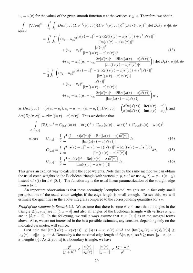
uv = u(v) for the values of the given smooth function u at the vertices x, y, z. Therefore, we obtain∫∆[x,y,z]

|∇ITu|2 =∫ 1

0

∫ 1

0Du∆(τ, σ)Dp−1(p(τ, σ))(Dp−1(p(τ, σ)))T (Du∆(τ, σ))T | detDp(τ, σ)|dτdσ

=∫ 1

0

∫ 1

0

((uz − uy)2 |s(τ)− x|2 − 2τRe((s(τ)− x)s′(τ)) + τ 2|s′(τ)|2

|Im((s(τ)− x)s′(τ))|2

+ (uy − ux)2 |s′(τ)|2

|Im((s(τ)− x)s′(τ))|2(13)

+(uy − ux)(uz − uy)2τ |s′(τ)|2 − 2Re((s(τ)− x)s′(τ))

|Im((s(τ)− x)s′(τ))|2

)| detDp(τ, σ)|dτdσ

=1

2

∫ 1

0

((uz − uy)2 |s(τ)− x|2 − 2τRe((s(τ)− x)s′(τ)) + τ 2|s′(τ)|2

|Im((s(τ)− x)s′(τ))|

+ (uy − ux)2 |s′(τ)|2

|Im((s(τ)− x)s′(τ))|

+(uy − ux)(uz − uy)2τ |s′(τ)|2 − 2Re((s(τ)− x)s′(τ))

|Im((s(τ)− x)s′(τ))|

)dτ,

asDu∆(τ, σ) = (σ(uz − uy), uy − ux + τ(uz − uy)),Dp(τ, σ) =

ÇσRe(s′(τ)) Re(s(τ)− x)σIm(s′(τ)) Im(s(τ)− x)

å, and

det(Dp(τ, σ)) = σIm((s(τ)− x)s′(τ)). Thus we deduce that∫∆[x,y,z]

|∇ITu|2 = C[x,y](u(x)− u(y))2 + C[y,z](u(y)− u(z))2 + C[z,x](u(z)− u(x))2,

where C[x,y] =1

2

∫ 1

0

(1− τ)|s′(τ)|2 + Re((s(τ)− x))s′(τ))

|Im((s(τ)− x)s′(τ))|dτ, (14)

C[y,z] =1

2

∫ 1

0

|s(τ)− x|2 + τ(τ − 1)|s′(τ)|2 + Re((s(τ)− x)s′(τ))

|Im((s(τ)− x)s′(τ))|dτ, (15)

C[z,x] =1

2

∫ 1

0

τ |s′(τ)|2 − Re((s(τ)− x)s′(τ))

|Im((s(τ)− x)s′(τ))|dτ. (16)

This gives an explicit way to calculate the edge weights. Note that by the same method we can obtainthe usual cotan-weights on the Euclidean triangle with vertices x, y, z, if we use sE(t) = y+ t(z− y)instead of s(t) for t ∈ [0, 1]. The function sE is the usual linear parametrization of the straight edgefrom y to z.

An important observation is that these seemingly ’complicated’ weights are in fact only smallperturbations of the usual cotan-weights if the edge length is small enough. To see this, we willestimate the quantities in the above integrals compared to the corresponding quantities for sE .

Proof of the estimate in Remark 2.2. We assume that there is some δ > 0 such that all angles in thetriangle ∆[x, y, z] are in [δ, π − δ] and also all angles of the Euclidean triangle with vertices x, y, zare in [δ, π − δ]. In the following, we will always assume that τ ∈ [0, 1] as in the integral termsabove. Also, we are not interested in the best possible estimates, any constant, depending only on theindicated parameter, will suffice.

First note that |Im((s(τ) − x)s′(τ))| ≥ |s(τ) − x||s′(τ)| sin δ and |Im((sE(τ) − x)s′E(τ))| ≥|sE(τ)−x||z− y| sin δ. Denote by h the maximal edge length of ∆[x, y, z], so h ≥ max|y−x|, |z−x|, length(s). As ∆[x, y, z] is a boundary triangle, we have

%2

(%+ h)2≤∣∣∣∣∣ s′(τ)

sE(τ)

∣∣∣∣∣ =|s′(τ)||y − z|

≤ (%+ h)2

%2.

20

Furthermore, we deduce that 1− Constδ,% · h ≤∣∣∣ s(τ)−xsE(τ)−x

∣∣∣ ≤ 1 + Constδ,% · h as∣∣∣∣∣s(τ)− sE(τ)

sE(τ)− x

∣∣∣∣∣ =

∣∣∣∣∣τ(τ − 1)(y − z)2

z + τ(y − z)· 1

(y − x) + τ(z − y)

∣∣∣∣∣ ≤ h

% sin2 δ.

Further, note that using the sine law

sin2 δ ≤ |sE(τ)− x||s′E(τ)|

=|(y − x) + τ(z − y)|

|y − z|≤ 1 +

1

sin δ.

Combining these estimates, we have

|s(τ)− sE(τ)||s′(τ)||Im((sE(τ)− x)s′E(τ))|

≤ |s(τ)− sE(τ)||sE(τ)− x|

·∣∣∣∣∣ s′(τ)

sE(τ)

∣∣∣∣∣ · 1

sin δ≤ Constδ,% · h,

|s′(τ)|2

|Im((sE(τ)− x)s′E(τ))|≤∣∣∣∣∣ s′(τ)

sE(τ)

∣∣∣∣∣ · |s′E(τ)|2

|s′E(τ)||sE(τ)− x| sin δ≤ Constδ,% · h,

|s(τ)− x|2

|Im((sE(τ)− x)s′E(τ))|≤ |s(τ)− x|2

|sE(τ)− x|2· |sE(τ)− x|2

|s′E(τ)||sE(τ)− x| sin δ≤ Constδ,% · h.

Furthermore, as h ≤ %/2,

|sE(τ)− x||s′(τ)− s′E(τ)||Im((sE(τ)− x)s′E(τ))|

≤ |s′(τ)− s′E(τ)||y − z| sin δ

=|y − z||τ 2(y − z)2 + 2τz − z||z + τ(y − z)|2 sin δ

≤ 6

% sin δ· h.

Therefore, we obtain∣∣∣∣∣∣ Im((s(τ)− x)s′(τ))

Im((sE(τ)− x)s′E(τ))− 1

∣∣∣∣∣∣=

∣∣∣∣∣∣ Im((s(τ)− sE(τ))s′(τ))

Im((sE(τ)− x)s′E(τ))+

Im((s(τ)− x)(s′(τ)− s′E(τ)))

Im((sE(τ)− x)s′E(τ))

∣∣∣∣∣∣ ≤ Const%,δ · h∣∣∣∣∣∣Re((s(τ)− x)s′(τ))− Re((sE(τ)− x)s′E(τ))

Im((sE(τ)− x)s′E(τ))

∣∣∣∣∣∣=

∣∣∣∣∣∣Re((s(τ)− sE(τ))s′(τ))

Im((sE(τ)− x)s′E(τ))+

Re((sE(τ)− x)(s′(τ)− s′E(τ)))

Im((sE(τ)− x)s′E(τ))

∣∣∣∣∣∣ ≤ Const′%,δ · h

This also implies∣∣∣∣ Re((s(τ)−x)s′(τ))

Im((sE(τ)−x)s′E(τ))

∣∣∣∣ ≤ ∣∣∣∣Re((sE(τ)−x)s′E(τ))

Im((sE(τ)−x)s′E(τ))

∣∣∣∣ + Const′%,δ · h ≤ Const′′%,δ Denote by αEz ∈[δ, π − δ] the angle in the Euclidean triangle with vertices x, y, z. Then the previous estimates imply

|C[x,y] −1

2cotαEz | ≤

1

2

∫ 1

0

Ü(1− τ)(|s′(τ)|2

∣∣∣∣ Im((s(τ)−x)s′(τ))

Im((sE(τ)−x)s′E(τ))− 1

∣∣∣∣+ ∣∣∣∣ |s′(τ)|2|s′E(τ)|2 − 1

∣∣∣∣ |s′E(τ)|2)

|Im((sE(τ)− x)s′E(τ))|

+|Re((s(τ)− x)s′(τ))|

∣∣∣∣ Im((s(τ)−x)s′(τ))

Im((sE(τ)−x)s′E(τ))− 1

∣∣∣∣|Im((sE(τ)− x)s′E(τ))|

+|Re((s(τ)− x)s′(τ))− Re((sE(τ)− x)s′E(τ))|

|Im((sE(τ)− x)s′E(τ))|

)dτ

≤ Const′′′%,δ · h.

Similarly, we can deduce that |C[y,z]− 12

cotαEx | ≤ Const′′′%,δ ·h and |C[z,x]− 12

cotαEy | ≤ Const′′′%,δ ·h.

21

A.2 Proof of Lemma 3.10Note that as u is smooth, there exist constants Constu,%, constu,% > 0 such that for 0 < h < constu,%we have |u(x)− u(y)|2/|x− y|2 ≤ Constδ,% ·max

w∈∆‖D1u(w)‖2 ≤ Constu,% for all edges e = [x, y] of

boundary triangles in F% with edge lengths smaller than h.Using our estimates of Section A.1 we deduce that there exists a constant Constδ,% such that under

our assumptions on angles and edge lengths we have the following estimates: For every boundarytriangle ∆[x, y, z] ∈ F% and with the notation of Section A.1

|z − y|2 |s(τ)− x|2

|Im((s(τ)− x)s′(τ))|2≤ Constδ,%,

|y − x|2 |s′(τ)|2

|Im((s(τ)− x)s′(τ))|2≤ Constδ,%,

|y − x||z − y| |Re((s(τ)− x)s′(τ))||Im((s(τ)− x)s′(τ))|2

≤ Constδ,%.

Now formula (13) leads to the estimate∫∆[x,y,z]

|∇ITu|2 ≤ Constδ,%,u · Area(∆[x, y, z]), (17)

where Constδ,%,u ≤ Constδ,% ·maxw∈∆‖D1u(w)‖2. Summing up these energies, we obtain

EF%(u) =∑

∆∈F%ET∆

(u) =∑

∆∈F%

∫∆[x,y,z]

|∇ITu|2 ≤∑

∆∈F%Constδ,%,u · Area(∆[x, y, z])

≤ Constδ,%,u · Area(B%+h(0) \B%−h(0)) ≤ Constδ,%,u · 4h% · d ≤ Constu,δ,%,R · h,

where d denotes the degree of the covering map forR.

A.3 Proof of Equicontinuity Lemma 4.1First note that condition (D) from Section 2.4 implies that for every path in a non-degenerate uniformadapted triangulation T with consecutive vertices v0v1 . . . vm we have

Ev0v1...vm(u) :=m∑k=1

c([vk−1, vk]) · (u(vk)− u(vk−1))2 ≥m∑k=1

Const

e· (u(vk)− u(vk−1))2

≥ Const

e· 1

m

(m∑k=1

u(vk)− u(vk−1)

)2

=Const

e ·m(u(vm)− u(v0))2. (18)

Here e denotes the eccentricity as defined in Section 4.1 and for the last estimate we have usedSchwarz’s inequality.

Now consider a simply connected triangulation T ′ with boundary contained in an open discBr(v) ⊂ C. This is the assumption for part (i) of the lemma. In the case of part (ii), we considerthe image triangulation T ′g by the chart gO(z) = (z − O)γO . By abuse of notation, we still denotethis image triangulation by T ′. Also, we denote the vertices of T ′ by Z andW , which are the actualvertices z, w in the first case and the images Z = gO(z), W = gO(w) in the case of a branch point.For simplicity, we assume that the edges between vertices are straight line segments, as we do notneed the actual, possibly curved edges.

Let u : V ′ → R be any function which assumes its maximum and its minimum on the boundaryfor any subgraph of T ′. Let Z,W be two distinct interior vertices of T ′. Denote by ZW the straight

22

line segment joining these points. Let dist(ZW, ∂T ′) be the Euclidean distance of this straight linesegment to the curve of boundary edges. We assume that |Z−W | < r/3 < dist(ZW, ∂T ′)/3 for somer > 0. Let h′ denote twice the maximum circumradius of the triangles of T ′. Letm = b r−|Z−W |

2h′c be

the largest integer smaller than r−|Z−W |2h′

. We consider auxiliary rectangles Rk, k = 1, . . . ,m, whichare centered at (Z +W )/2 with one pair of sides parallel to ZW with length ZW + 2k · h′ and otherpair of sides orthogonal to ZW of length 2k · h′. Then the interior of Rk, k = 1, . . . ,m, is coveredby triangles of T ′. Denote by V ′k the set of vertices contained in Rk \ Rk−1, where R0 = ZW . Thenany two vertices vA, vB ∈ V ′k may be connected by a path v0v1 . . . vN with v0 = vA, vN = vB and allvertices vj ∈ V ′k as h′ is larger than any edge length.

Without loss of generality, assume that u(Z) ≥ u(W ). As u assumes its maximum and minimumon the boundary, there exists Zk,Wk ∈ V ′k such that u(Zk) ≥ u(Z) ≥ u(W ) ≥ u(Wk). The length ofthe path joining Zk and Wk is at most the number of vertices in V ′k . The set of these vertices can becovered by at most Const · (|Z −W |+ 4kh′)/h′ discs of radius h′/2. Therefore, by condition (U) ofSection 2.4 the number of vertices in V ′k is less than Const · e · (|Z −W |/h′ + 4k). Therefore, we canestimate the energy for a path v0v1 . . . vN in V ′k from v0 = Zk, vN = Wk using (18)

EZk...Wk(u) ≥ Const

e · (Const · e · (|Z −W |/h′ + 4k))· (u(Zk)− u(Wk))

2

= Const · (u(Z)− u(W ))2

e2· h′

km′ + |Z −W |/4.

Summing these estimates and estimating∑mk=1

h′

kh′+|Z−W |/4 ≥ Const∫ r−|Z−W |

2h′

dtt+|Z−W |/4 we get

E ′(u) ≥m∑k=1

EZk...Wk(u) ≥ Const · (u(Z)− u(W ))2

e2·∫ r−|Z−W |

2

h′

dt

t+ |Z −W |/4

≥ Const · (u(Z)− u(W ))2

e2· log

2r − |Z −W |4h′ + |Z −W |

≥ Const · (u(Z)− u(W ))2

e2· log

r

3 max|Z −W |, h′.

This implies the desired inequalities (9) and (10).

References[BG16] Alexander I. Bobenko and Felix Günther, Discrete complex analysis on planar quad-

graphs, Advances in discrete differential geometry, Springer, 2016, pp. 57–132.

[BG17] ,Discrete Riemann surfaces based on quadrilateral cellular decompositions, Adv.Math. 311 (2017), 885–932.

[BMS05] A. I. Bobenko, Ch. Mercat, and Yu. B. Suris, Linear and nonlinear theories of discreteanalytic functions. Integrable structure and isomonodromic Green’s function, J. reineangew. Math. 583 (2005), 117–161.

[BMS11] A. I. Bobenko, Ch. Mercat, and M. Schmies, Period matrices of polyhedral surfaces,Computational Approach to Riemann Surfaces (A. I. Bobenko and Ch. Klein, eds.), vol.2013, Springer, 2011, pp. 213–226.

[BP96] A. I. Bobenko and U. Pinkall, Discrete isothermic surfaces, J. Reine Angew. Math. 475(1996), 187–208.

23

[BPS15] A.I. Bobenko, U. Pinkall, and B. Springborn, Discrete conformal maps and ideal hyper-bolic polyhedra, Geom. Topol. 19 (2015), no. 4, 2155–2215.

[BS04] A. I. Bobenko andB.A. Springborn,Variational principles for circle patterns andKoebe’stheorem, Trans. Amer. Math. Soc. 356 (2004), 659–689.

[BS16] A. I. Bobenko and M. Skopenkov, Discrete Riemann surfaces: linear discretization andits convergence, J. Reine Angew. Math. 720 (2016), 217–250.

[Büc08] U. Bücking, Approximation of conformal mappings by circle patterns, Geom. Dedicata137 (2008), 163–197.

[Büc16] , Approximation of conformal mappings on triangular lattices, Advances in Dis-crete Differential Geometry (A.I. Bobenko, ed.), Springer, 2016.

[CFL28] R. Courant, K. Friedrichs, and H. Lewy, Über die partiellen Differentialgleichungen dermathematischen Physik, Math. Ann. 100 (1928), 32–74.

[CS11] D. Chelkak and St. Smirnov,Discrete complex analysis on isoradial graphs, Adv. inMath.228 (2011), no. 3, 1590 – 1630.

[DN03] I.A. Dynnikov and S.P. Novikov, Geometry of the triangle equation on two-manifolds,Mosc. Math. J. 3 (2003), 419–438.

[Duf53] R. J. Duffin, Discrete potential theory, Duke Math. J. 20 (1953), 233–251.

[Duf56] , Basic properties of discrete analytic functions, Duke Math. J. 23 (1956), 335–363.

[Duf59] , Distributed and lumped networks, J. Math. Mech. 8 (1959), 793–826.

[Duf68] , Potential theory on a rhombic lattice, J. Combin. Th. 5 (1968), 258–272.

[DvH01] B. Deconinck and M. van Hoeij, Computing Riemann matrices of algebraic curves,Physica D 152-153 (2001), 28 – 46, Advances in Nonlinear Mathematics and Science: ASpecial Issue to Honor Vladimir Zakharov.

[Fer44] J. Ferrand, Fonctions préharmoniques et fonctions préholomorphes, Bull. Sci. Math. 68(1944), 152–180.

[FK15] J. Frauendiener and Ch. Klein, Computational approach to hyperelliptic Riemann sur-faces, Lett. Math. Phys. 105 (2015), no. 3, 379–400.

[FK17] , Computational approach to compact Riemann surfaces, Nonlinearity 30 (2017),no. 1, 138–172.

[GSST98] P. Gianni, M. Seppälä, R. Silhol, and B. Trager, Riemann surfaces, plane algebraic curvesand their period matrices, J. Symbolic Comput. 26 (1998), no. 6, 789 – 803.

[Isa41] R. Ph. Isaacs, A finite difference function theory, Univ. Nac. Tucumán Revista A 2 (1941),177–201.

[LF55] J. Lelong-Ferrand, Représentation confrome et transformations à intégrale de Dirichletbornée, Gauthier-Villars, Paris, 1955.

[Lus26] L. Lusternik,Über einige Anwendunge der direkten Methoden in der Variationsrechnung,Mat. Sb. 33 (1926), no. 2, 173–201.

24

[Mac49] R.MacNeal, The solution of partial differential equations by means of electrical networks,Ph.D. thesis, California Institute of Technology, 1949.

[Mat05] D.Matthes, Convergence in discrete Cauchy problems and applications to circle patterns,Conform. Geom. Dyn. 9 (2005), 1–23.

[MDSB03] M. Meyer, M. Desbrun, P. Schröder, and A. H. Barr, Discrete differential geometryoperators for triangulated 2-manifolds, Visualization and Mathematics III, Springer,2003, pp. 35–57.

[Mer01] Ch. Mercat, Discrete Riemann surfaces and the Ising model, Commun. Math. Phys. 218(2001), 177–216.

[Mer02] , Discrete period matrices and related topics, e-print arXiv:math-ph/0111043,2002.

[Mer07] ,Discrete Riemann surfaces, Handbook of Teichmüller Theory (A. Papadopoulos,ed.), IRMA Lectures in Mathematics and Theoretical Physics, vol. 11, Eur. Math. Soc.,2007, pp. 541–575.

[MN17] P. Molin and C. Neurohr, Computing period matrices and the Abel-Jacobi map of su-perelliptic curves, e-print arXiv:1707.07249 [math.NT], 2017.

[Nov11] S.P. Novikov, New discretization of complex analysis: the Euclidean and Hyperbolicplanes, Proceedings of the Steklov Institute of Mathematics 273 (2011), 238–251.

[PP93] U. Pinkall and K. Polthier, Computing discrete minimal surfaces and their conjugates,Experiment. Math. 2 (1993), 15–36.

[Sch97] O. Schramm, Circle patterns with the combinatorics of the square grid, Duke Math. J. 86(1997), 347–389.

[Sko13] M. Skopenkov, The boundary value problem for discrete analytic functions, Adv. Math.240 (2013), 61–87.

[Ste05] K. Stephenson, Introduction to circle packing: the theory of discrete analytic functions,Cambridge University Press, New York, 2005.

25