Computational Statistics & Data Analysis 41 (2002) 171–184www.elsevier.com/locate/csda

On good matrices, skew Hadamard matrices andoptimal designs

S. Georgiou, C. Koukouvinos∗, S. StylianouDepartment of Mathematics, National Technical University of Athens, Zografou 15773, Athens, Greece

Abstract

In two-level factorial experiments and in other linear models the coe.cients of the unknownparameters can take one out of two values. When the number of observations is a multiple offour, the D-optimal design is a Hadamard matrix. Skew Hadamard matrices are of special interestdue to their use, among others, in constructing D-optimal weighing designs for n ≡ 3 (mod 4).A method is given for constructing skew Hadamard matrices which is based on the constructionof good matrices. The construction is achieved through an algorithm which is also presented andrelies on the discrete Fourier transform.

It is known that good matrices of order n; exist for all odd n6 35 and n= 127: In this paper,we give for the 6rst time all non-equivalent circulant good matrices of odd order 336 n6 39:We note that no good matrices were previously known for orders 37 and 39: These are presentedin a table in the form of the corresponding non-equivalent supplementary di9erence sets. In thesequel we use good matrices to construct some skew Hadamard matrices and orthogonal designs.c© 2002 Elsevier Science B.V. All rights reserved.

Keywords: Good matrices; Supplementary di9erence sets; Skew Hadamard matrices; Linear models;Optimal designs; Orthogonal designs

1. Introduction

In certain linear models the coe.cients of the unknown parameters can take one outof two values, which can be taken as +1 and −1: The problem we face is how todesign the experiment so that the estimators of the unknown parameters are “e.cient”in some sense.

∗ Corresponding author.E-mail address: ckoukouv@math.ntua.gr (C. Koukouvinos).

0167-9473/02/$ - see front matter c© 2002 Elsevier Science B.V. All rights reserved.PII: S0167 -9473(02)00067 -1

172 S. Georgiou et al. / Computational Statistics & Data Analysis 41 (2002) 171–184

To be more precise, suppose we have the linear model

yi = xi1b1 + · · · + xikbk + ei; i = 1; : : : ; n;

where the errors ei are uncorrelated with zero mean and common variance 2:The n× k matrix X = (xij); i= 1; : : : ; n; j= 1; : : : ; k; is called the design matrix and

the k × k matrix M = X TX is called its information matrix, where T indicates thetranspose.

The covariance matrix of the linear least-squares estimator b̂ of b is 2M−1 and inconstructing optimal designs we minimize a given function of M: In this paper we areinterested in minimizing the generalized variance, i.e., maximizing the determinant ofM over all possible designs X: This is called D-optimality.

In the particular case where we have k factors, each at two levels, then xij = +1 or−1 whenever in the ith observation factor j enters at the high level or at the low level.A similar situation arises in weighing experiments with a chemical balance when theobjects are put on the right or the left scale-pan.

There exist algorithms (Fedorov, 1972, p. 97; Wynn, 1970) for constructing D-optimalcontinuous designs where the optimal observation points and the optimal proportion ofobservations at these points are found. However, if we want these observations to bemultiples of 1=n; where n is the number of observations, the algorithms do not alwaysconverge to the global maximum due to the existence of many local optima.

In this paper we only consider experiments where xij = ±1; then if the numberof observations is a multiple of four, i.e., n ≡ 0 (mod 4); detM is maximized whenthe columns of the design X are orthogonal to each other. If k = n the design iscalled saturated and the D-optimal design is a Hadamard matrix of order n, whenevern ≡ 0 (mod 4).

So the construction of Hadamard matrices of order n gives D-optimal n-observationdesigns. Plackett and Burman (1946), in studying optimal multifactorial experiments,constructed Hadamard matrices for orders n6 100; n ≡ 0 (mod 4). They omitted thecase n= 92, which was later provided by Baumert et al. (1962).

A great deal of research has been devoted in constructing Hadamard matrices andstudying their properties. For more details we refer the reader to Geramita and Seberry(1979), Seberry Wallis (1972) and Seberry and Yamada (1992).

Skew Hadamard matrices are of special interest since, among others, they are used inconstructing D-optimal weighing designs for n ≡ 0 (mod 4); see for example Kouniasand Chadjipantelis (1983).

Hadamard matrices is a special case of orthogonal designs. In this paper, we studygood matrices and their use in the construction of skew Hadamard matrices and or-thogonal designs.

2. Orthogonal designs and good matrices

An orthogonal design of order n and type (s1; s2; : : : ; su) (si ¿ 0), denoted OD(n; s1; s2; : : : ; su), on the commuting variables x1; x2; : : : ; xu is an n × n matrix A with

S. Georgiou et al. / Computational Statistics & Data Analysis 41 (2002) 171–184 173

entries from {0;±x1;±x2; : : : ;±xu} such that

AAT =

(u∑i=1

six2i

)In:

Alternatively, the rows of A are formally orthogonal and each row has precisely sientries of the type ±xi. In Geramita et al. (1976) where this was 6rst de6ned, it wasmentioned that

ATA=

(u∑i=1

six2i

)In

and so our alternative description of A applies equally well to the columns of A. It wasalso shown in Geramita et al. (1976) that u6 �(n), where �(n) (Radon’s function) isde6ned by �(n) = 8c + 2d, when n= 2ab; b odd, a= 4c + d; 06d¡ 4.

A (1;−1) matrix of order n is called a Hadamard matrix if HHT =HTH=nIn, whereHT is the transpose of H and In is the identity matrix of order n. Thus, a Hadamardmatrix of order n can be considered as an OD(n; n): A (1;−1) matrix A of order nis said to be of skew type if A− In is skew symmetric. Two (1;−1) matrices A; B oforder n are said to be amicable if ABT = BAT:

Let G be an additive abelian group of order n with elements g1; g2; : : : ; gn and X asubset of G. De6ne the type 1 (1;−1) incidence matrix M = (mij) of order n of X tobe

mij =

{+1 if gj − gi ∈X;−1 otherwise:

and the type 2 (1;−1) incidence matrix N = (nij) of order n of X to be

nij =

{+1 if gj + gi ∈X;−1 otherwise:

In particular, if G is cyclic the matrices M and N are called circulant and back circulant,respectively. In this case mij =m1; j−i+1 and nij = n1; i+j−1, respectively (indices shouldbe reduced modulo n).

De�nition 1. Let X1; X2; X3; X4 be four (1;−1) matrices of order n (odd) with theproperties:

(i) (X1 − I)T = −(X1 − I);(ii) X T

i = Xi; i = 2; 3; 4;(iii) XiX T

j = XjX Ti ;

(iv) X1X T1 + X2X T

2 + X3X T3 + X4X T

4 = 4nIn.

Call such matrices good matrices of order n.

De�nition 2. Four {±1}-matrices X1; X2; X3; X4 are called 4-Williamson type matricesif X1; X2; X3; X4 are pairwise amicable and satisfy

X1X T1 + X2X T

2 + X3X T3 + X4X T

4 = 4nIn:

174 S. Georgiou et al. / Computational Statistics & Data Analysis 41 (2002) 171–184

If X1; X2; X3; X4 are good matrices then X1; X2; X3; X4 are obviously 4-Williamson typematrices as well.

Williamson type matrices are of paramount importance in the constructions ofHadamard matrices, see Seberry Wallis (1975), Seberry Wallis (1975). Given 4-Williamson type matrices of order n one can construct a Hadamard matrix of or-der 4nt for in6nitely many odd values of t. The permissible values of t are those forwhich there exist Baumert–Hall arrays of order 4t, see Geramita and Seberry (1979)for details. Good matrices can be used to construct new 4-Williamson type matrices,as indicated in Section 4.

In the present paper we are dealing with good matrices which are circulant. Hence,multiplying on the left by eT (the 1 × n vector of one’s) and on the right by e bothsides of (iv) we conclude that circulant good matrices can only exist for orders n ofwhich 4n = 12 + a2 + b2 + c2, where a; b; c are the sums of the elements of the 6rstrow of symmetric matrices X2, X3 and X4, respectively, and they are odd integers. Allnon-equivalent circulant good matrices of order n, were known for all odd n6 31,see Szekeres (1988), and some solutions were known for n= 33; 35; 127, see Djokovic(1993).

Let U be a sequence of n real numbers u0; u1; : : : ; un−1. The periodic autocorrelationfunction PU (j) of such a sequence is de6ned, reducing the subscript i + j modulo n,as

PU (j) =n−1∑i=0

uiui+j; j = 0; 1; : : : ; n− 1:

Four sequences A; B; C and D of identical length n are said to be compatible if thesum of their periodic autocorrelations is a constant, say a, except for the 0th term.That is

PA(j) + PB(j) + PC(j) + PD(j) = a; j = 0: (1)

Such sequences are said to have constant periodic autocorrelation even though it isthe sum of the autocorrelations that is a constant.

In this paper we give for the 6rst time all non-equivalent circulant good matrices ofodd order n=33; 35; 37 and 39. We note that no good matrices were previously knownfor orders 37 and 39. Thus, the 6rst open case is n= 41:

In Section 3 we describe brieMy the method of construction, in Section 4 we usegood matrices to construct some skew Hadamard matrices and orthogonal designs, andin Section 5 we present in Table 2 the new results.

3. Method of construction—the algorithm

3.1. Some preliminary results

In order to describe our construction of good matrices we need a few more de6ni-tions. Let n be a positive integer.

S. Georgiou et al. / Computational Statistics & Data Analysis 41 (2002) 171–184 175

De�nition 3. Four subsets S0; S1; S2; S3 of {1; 2; : : : ; n−1} are called 4-(n; n0; n1; n2; n3; &)supplementary di9erence sets (sds) modulo n if |Sk |= nk for k = 0; 1; 2; 3 and for eachm∈{1; 2; : : : ; n− 1} we have &0(m) + · · · + &3(m) = &; where &k(m) is the number ofsolutions (i; j) of the congruence i − j ≡ m (mod n) with i; j∈ Sk .

Suppose that Sk are 4-(n; n0; n1; n2; n3; &) sds modulo n having the following addi-tional properties:

n+ &= n0 + n1 + n2 + n3; (2)

i∈ S0 ⇔ n− i ∈ S0; (3)

i∈ St ⇔ n− i∈ St ; t = 1; 2; 3; (4)

where in (3) and (4) it is assumed that i∈{1; 2; : : : ; n− 1}:Let ak = (ak0 ; ak1 ; : : : ; akn−1 ); k = 0; 1; 2; 3; be the row vector de6ned by

aki ={−1 if i∈ Sk ;

1 otherwise:

Furthermore, let A0 be the circulant matrix with 6rst row a0, and let Ak; k = 1; 2; 3, bethe back-circulant matrix with 6rst row ak . Then it is well known (and can be easilyveri6ed) that A0; A1; A2; A3 are good matrices of order n:

Let r be an integer relatively prime to n, and set

S ′k = {ri (mod n): i∈ Sk} ⊂ {1; 2; : : : ; n− 1}for k = 0; 1; 2; 3: These sets are also 4-(n; n0; n1; n2; n3; &) sds modulo n satisfying con-ditions (2)–(4). We shall say that such quadruples S0; S1; S2; S3 and S ′0; S

′1; S

′2; S

′3 are

equivalent.The discrete Fourier transform (DFT) of a sequence B with elements b0; b1; : : : ; bn−1,

is given by

DFTB(k) = *Bk =n−1∑i=0

bi!ik ; k = 0; 1; : : : ; n− 1;

where ! is a primitive ‘th root of unity e2-i=‘. If we take the squared magnitude ofeach term in the DFT of B, the resulting sequence is called the power spectral density(PSD) of B and will be denoted by *2

Bk .We make use of the following well-known theorem (see Press et al., 1981, Chapter

12; Tretter, 1976, Chapter 10).

Theorem 1 (Wiener–Khinchin). Let B be a sequence of length n with elements fromthe set {0;±1}: The PSD of this sequence is equal to the DFT of its periodic auto-correlation function

|*Bk |2 =n−1∑j=0

PB(j)!jk : (5)

176 S. Georgiou et al. / Computational Statistics & Data Analysis 41 (2002) 171–184

The periodic autocorrelation function is equal to the inverse DFT of the sequence’sPSD

PB(j) =1‘

n−1∑k=0

|*Bk |2!−jk : (6)

Example 1. Let A= {1;−1; 0; 0;−1;−1;−1; 0; 1}. Then the PSD of A is

4:000 11:596 8:042 4:000 1:362 1:362 4:000 8:042 11:596

A similar technique but using two sequences was also applied in Fletcher et al.(2001).

Our main theorem is

Theorem 2. Four sequences are compatible if and only if their PSDs sum to a con-stant.

Proof. By straightforward application of (1); (5) and (6); we have

|*Ak |2 + |*Bk |2 + |*Ck |2 + |*Dk |2

=n−1∑j=0

(PA(j) + PB(j) + PC(j) + PD(j))!jk

= (PA(0) + PB(0) + PC(0) + PD(0) − a)!0 +n−1∑j=0

a!jk

= c (k = 0);

PA(j) + PB(j) + PC(j) + PD(j)

=1n

n−1∑k=0

(|*Ak |2 + |*Bk |2 + |*Ck |2 + |*Dk |2)!−jk

=1n

(|*A0 |2 + |*B0 |2 + |*C0 |2 + |*D0 |2 − c)!0 +1n

n−1∑k=0

c!−jk

= a (j = 0):

The inequalities k = 0 and j = 0 are required only in the 6nal steps of the aboveequations in order to force the rightmost sums to vanish.

Corollary 1. If PA(j) + PB(j) + PC(j) + PD(j) = 0 ∀j = 0 then

c =

(n−1∑i=0

ai

)2

+

(n−1∑i=0

bi

)2

+

(n−1∑i=0

ci

)2

+

(n−1∑i=0

di

)2

:

S. Georgiou et al. / Computational Statistics & Data Analysis 41 (2002) 171–184 177

Example 2. Four compatible sequences (with c=198) and their PSDs are shown below.Sequences, n = 11 PSD (terms 1–5)

1; 1;−1;−1; 3;−1;−1; 4;−1;−1;−4 26.21280 30.76150 113.78854 47.99641 50.240751;−1;−4;−1; 1;−1;−1;−3;−1;−1; 4 30.40560 152.59566 21.13192 0.81892 40.04790

1; 1;−2;−1;−1;−4; 1;−1; 1;−1; 4 101.43828 7.90167 33.49208 6.17342 90.994551; 1;−1; 1;−4;−1;−1;−4;−1; 1;−4 39.94332 6.74117 29.58746 143.01125 16.71680

198.00000 198.00000 198.00000 198.00000 198.00000

In fact, the constant c depends only on the set of numbers comprising the sequencesA; B; C and D. It is easily shown that

c =n∑n−1

i=0 (a2i +b

2i +c

2i +d

2i )−(

∑n−1i=0 ai)2 − (

∑n−1i=0 bi)2−(

∑n−1i=0 ci)2−(

∑n−1i=0 di)2

n− 1:

(7)

If we are dealing with four {±1} sequences of length n; then from above Eq. (7) wehave that c = (4n2 − 4n)=(n− 1) = (4n(n− 1))=(n− 1) = 4n:

In general we have

Remark 1. If A; B; C; and D are 0;±1 sequences then the above constant c is c=w−a;where w is the total number of non-zero entries and a is the constant from the periodicautocorrelation function of A; B; C and D.

Remark 2. It is well known that if A = {a0; : : : ; an−1}; B = {b0; : : : ; bn−1}; C ={c0; : : : ; cn−1}; and D = {d0; : : : ; dn−1} are {±1} sequences of odd length n satisfyingcondition (1) with a=0 and moreover the conditions a0 =1; ai=−an−i ; i=1; 2; : : : ; n−1(i.e. sequence A is skew) and x0 = 1; xi = xn−i ; i = 1; 2; : : : ; n − 1 where x∈{b; c; d}(i.e. sequences B; C; D are symmetric) then the corresponding circulant matrix A andthe back-circulant matrices B; C; D; are good matrices.

From the above facts we can easily see that circulant good matrices can be investi-gated in both forms, i.e. as supplementary di9erence sets or as {±1} sequences.

3.2. The algorithm

The algorithm we describe herein gives a fast way to search for circulant goodmatrices in the form of four {±1} sequences of length n. Modi6ed versions of thisalgorithm can be used anywhere we need to 6nd compatible sequences with elementsreal numbers. This algorithm can perform both, a partial or exhaustive search. Thesteps of this algorithm are the following:Step 1: Find all possible decompositions of 4n − 1 into three square non-negative

numbers (4n − 1 = b2 + c2 + d2). Then 4n = 12 + b2 + c2 + d2: Knowing these wecan conclude the number of positive and negative elements for each sequence. For the6rst sequence, the skew sequence A; we have (n+1)=2 positive and (n−1)=2 negativeelements. For the X symmetric sequence we have x+ (n− x)=2 positive and (n− x)=2negative elements where X ∈{B; C; D} and x∈{b; c; d}:

178 S. Georgiou et al. / Computational Statistics & Data Analysis 41 (2002) 171–184

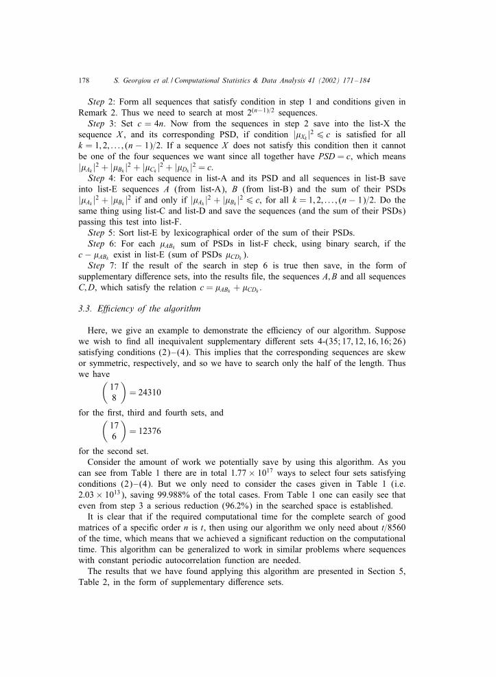
Step 2: Form all sequences that satisfy condition in step 1 and conditions given inRemark 2. Thus we need to search at most 2(n−1)=2 sequences.Step 3: Set c = 4n. Now from the sequences in step 2 save into the list-X the

sequence X , and its corresponding PSD, if condition |*Xk |26 c is satis6ed for allk = 1; 2; : : : ; (n − 1)=2: If a sequence X does not satisfy this condition then it cannotbe one of the four sequences we want since all together have PSD = c, which means|*Ak |2 + |*Bk |2 + |*Ck |2 + |*Dk |2 = c:Step 4: For each sequence in list-A and its PSD and all sequences in list-B save

into list-E sequences A (from list-A), B (from list-B) and the sum of their PSDs|*Ak |2 + |*Bk |2 if and only if |*Ak |2 + |*Bk |26 c; for all k = 1; 2; : : : ; (n− 1)=2: Do thesame thing using list-C and list-D and save the sequences (and the sum of their PSDs)passing this test into list-F.Step 5: Sort list-E by lexicographical order of the sum of their PSDs.Step 6: For each *ABk sum of PSDs in list-F check, using binary search, if the

c − *ABk exist in list-E (sum of PSDs *CDk ).Step 7: If the result of the search in step 6 is true then save, in the form of

supplementary di9erence sets, into the results 6le, the sequences A; B and all sequencesC;D, which satisfy the relation c = *ABk + *CDk .

3.3. E8ciency of the algorithm

Here, we give an example to demonstrate the e.ciency of our algorithm. Supposewe wish to 6nd all inequivalent supplementary di9erent sets 4-(35; 17; 12; 16; 16; 26)satisfying conditions (2)–(4). This implies that the corresponding sequences are skewor symmetric, respectively, and so we have to search only the half of the length. Thuswe have(

178

)= 24310

for the 6rst, third and fourth sets, and(176

)= 12376

for the second set.Consider the amount of work we potentially save by using this algorithm. As you

can see from Table 1 there are in total 1:77 × 1017 ways to select four sets satisfyingconditions (2)–(4). But we only need to consider the cases given in Table 1 (i.e.2:03 × 1013), saving 99:988% of the total cases. From Table 1 one can easily see thateven from step 3 a serious reduction (96:2%) in the searched space is established.

It is clear that if the required computational time for the complete search of goodmatrices of a speci6c order n is t, then using our algorithm we only need about t=8560of the time, which means that we achieved a signi6cant reduction on the computationaltime. This algorithm can be generalized to work in similar problems where sequenceswith constant periodic autocorrelation function are needed.

The results that we have found applying this algorithm are presented in Section 5,Table 2, in the form of supplementary di9erence sets.

S. Georgiou et al. / Computational Statistics & Data Analysis 41 (2002) 171–184 179

Table 1Total cases for 4-(35;17,12,16,16;26) sds

n= 35; 4-(35; 17; 12; 16; 16; 26)S0 S1 S2 S3

All cases 24310 12376 24310 24310

Cases after step 3 21995 5524 7390 7390

Cases after step 4 11820952 1757583

All cases in total (24310 × 24310) × (24310 × 12376)

= 177801400392616000 = 1:77 × 1017

Total cases after step 3 (21995 × 5524) × (7390 × 7390)

= 6635390902598000 = 6:63 × 1017

Total cases after step 4 1757583 × 11820952

= 20776304279016 = 2:07 × 1013

4. Constructions using good matrices

Good matrices can be used to construct new 4-Williamson type matrices. We mentiononly the following results of Seberry Wallis (1975).

Theorem 3. Suppose X; Y are (1;−1) matrices of order v such that

(i) XY T = YX T;(ii) XX T = (v− 4m+ 1)I + (4m− 1)J;

(iii) YY T = (v+ 1)I − J:

Further suppose A; B; C; D are good matrices of order m. Then A1; B1; C1; D1; of ordermv given by

A1 = I × X + (A− I) × Y;

B1 = B× Y;

C1 = C × Y;

D1 = D × Y

are 4-Williamson type matrices.

Corollary 2. Suppose there exist good matrices of order m: Then there exist4-Williamson type matrices of order m(4m− 1):

Corollary 3. Suppose there exist good matrices of order m: Further suppose 4m+ 4is the order of a symmetric Hadamard matrix. Then there exist 4-Williamson typematrices of order m(4m+ 3):

180 S. Georgiou et al. / Computational Statistics & Data Analysis 41 (2002) 171–184

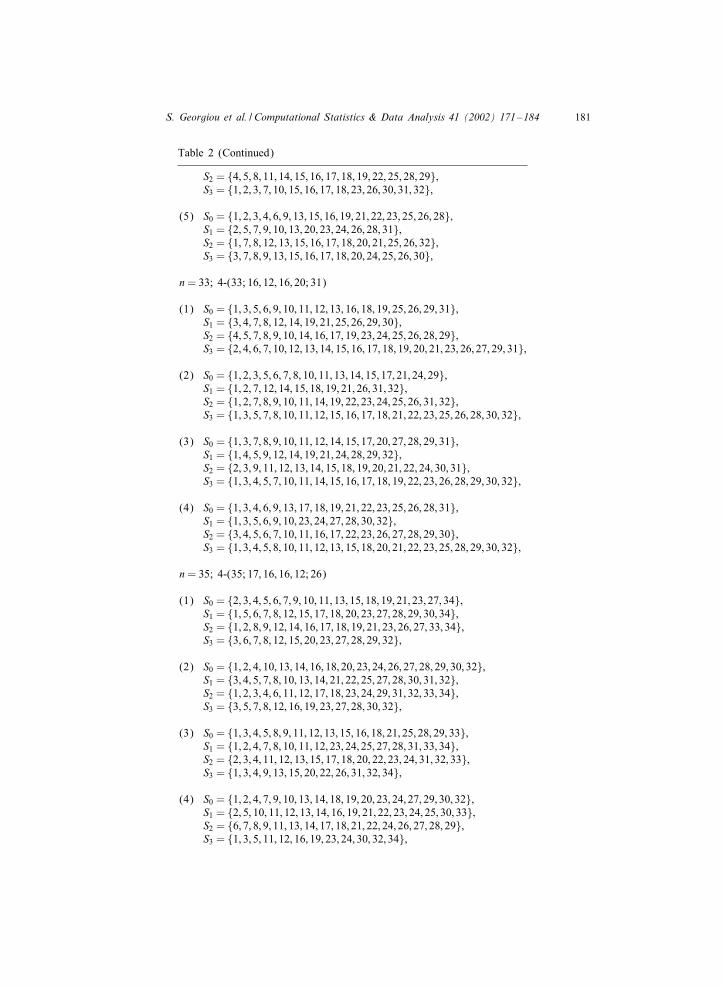
Table 2All non-equivalent circulant good matrices of odd orders 336 n6 39

n= 33; 4-(33; 16; 22; 16; 18; 39)

(1) S0 = {1; 2; 4; 5; 6; 7; 9; 10; 12; 16; 18; 19; 20; 22; 25; 30},S1 = {2; 3; 5; 6; 8; 10; 11; 12; 14; 15; 16; 17; 18; 19; 21; 22; 23; 25; 27; 28; 30; 31},S2 = {4; 5; 6; 8; 10; 11; 15; 16; 17; 18; 22; 23; 25; 27; 28; 29},S3 = {1; 3; 4; 5; 6; 9; 10; 12; 13; 20; 21; 23; 24; 27; 28; 29; 30; 32},

(2) S0 = {1; 2; 7; 8; 9; 11; 12; 14; 16; 18; 20; 23; 27; 28; 29; 30};S1 = {2; 4; 6; 7; 8; 9; 11; 12; 14; 15; 16; 17; 18; 19; 21; 22; 24; 25; 26; 27; 29; 31},S2 = {3; 6; 7; 8; 9; 11; 15; 16; 17; 18; 22; 24; 25; 26; 27; 30};S3 = {1; 2; 4; 5; 7; 8; 9; 12; 13; 20; 21; 24; 25; 26; 28; 29; 31; 32},

(3) S0 = {1; 2; 7; 9; 10; 11; 13; 14; 17; 18; 21; 25; 27; 28; 29; 30},S1 = {2; 3; 4; 6; 8; 9; 11; 12; 14; 15; 16; 17; 18; 19; 21; 22; 24; 25; 27; 29; 30; 31},S2 = {3; 5; 6; 11; 12; 14; 15; 16; 17; 18; 19; 21; 22; 27; 28; 30},S3 = {1; 2; 3; 5; 6; 7; 12; 14; 16; 17; 19; 21; 26; 27; 28; 30; 31; 32},

(4) S0 = {1; 3; 4; 5; 9; 11; 13; 16; 18; 19; 21; 23; 25; 26; 27; 31},S1 = {2; 3; 5; 6; 7; 8; 9; 11; 13; 14; 15; 18; 19; 20; 22; 24; 25; 26; 27; 28; 30; 31},S2 = {6; 7; 8; 10; 11; 13; 14; 16; 17; 19; 20; 22; 23; 25; 26; 27},S3 = {2; 3; 5; 6; 7; 12; 13; 14; 16; 17; 19; 20; 21; 26; 27; 28; 30; 31},

(5) S0 = {1; 2; 5; 6; 8; 9; 10; 12; 14; 15; 17; 20; 22; 26; 29; 30},S1 = {1; 2; 4; 5; 6; 8; 9; 13; 14; 15; 16; 17; 18; 19; 20; 24; 25; 27; 28; 29; 31; 32},S2 = {1; 2; 3; 4; 7; 9; 15; 16; 17; 18; 24; 26; 29; 30; 31; 32},S3 = {1; 3; 7; 8; 10; 13; 14; 15; 16; 17; 18; 19; 20; 23; 25; 26; 30; 32},

(6) S0 = {1; 5; 6; 8; 9; 10; 11; 12; 14; 15; 17; 20; 26; 29; 30; 31},S1 = {1; 2; 3; 4; 5; 7; 8; 9; 11; 14; 15; 18; 19; 22; 24; 25; 26; 28; 29; 30; 31; 32},S2 = {4; 5; 6; 7; 9; 12; 13; 14; 19; 20; 21; 24; 26; 27; 28; 29},S3 = {1; 3; 5; 8; 10; 11; 12; 13; 16; 17; 20; 21; 22; 23; 25; 28; 30; 32},

n= 33; 4-(33; 16; 12; 14; 14; 23)

(1) S0 = {1; 3; 5; 6; 9; 10; 11; 12; 13; 15; 16; 19; 25; 26; 29; 31};S1 = {1; 3; 5; 10; 11; 12; 21; 22; 23; 28; 30; 32};S2 = {3; 6; 7; 11; 12; 14; 15; 18; 19; 21; 22; 26; 27; 30};S3 = {1; 2; 3; 4; 10; 13; 15; 18; 20; 23; 29; 30; 31; 32};

(2) S0 = {1; 2; 3; 4; 5; 7; 9; 11; 12; 15; 17; 19; 20; 23; 25; 27};S1 = {5; 6; 7; 10; 12; 14; 19; 21; 23; 26; 27; 28};S2 = {1; 2; 7; 8; 11; 12; 14; 19; 21; 22; 25; 26; 31; 32};S3 = {5; 6; 10; 11; 13; 14; 16; 17; 19; 20; 22; 23; 27; 28};

(3) S0 = {3; 4; 5; 7; 9; 12; 13; 14; 15; 16; 22; 23; 25; 27; 31; 32};S1 = {2; 6; 8; 11; 13; 14; 19; 20; 22; 25; 27; 31};S2 = {1; 5; 6; 7; 8; 11; 15; 18; 22; 25; 26; 27; 28; 32};S3 = {2; 5; 10; 13; 14; 15; 16; 17; 18; 19; 20; 23; 28; 31};

(4) S0 = {1; 2; 3; 6; 7; 13; 15; 17; 19; 21; 22; 23; 24; 25; 28; 29};S1 = {2; 7; 9; 11; 14; 16; 17; 19; 22; 24; 26; 31};

S. Georgiou et al. / Computational Statistics & Data Analysis 41 (2002) 171–184 181

Table 2 (Continued)

S2 = {4; 5; 8; 11; 14; 15; 16; 17; 18; 19; 22; 25; 28; 29};S3 = {1; 2; 3; 7; 10; 15; 16; 17; 18; 23; 26; 30; 31; 32};

(5) S0 = {1; 2; 3; 4; 6; 9; 13; 15; 16; 19; 21; 22; 23; 25; 26; 28};S1 = {2; 5; 7; 9; 10; 13; 20; 23; 24; 26; 28; 31};S2 = {1; 7; 8; 12; 13; 15; 16; 17; 18; 20; 21; 25; 26; 32};S3 = {3; 7; 8; 9; 13; 15; 16; 17; 18; 20; 24; 25; 26; 30};

n= 33; 4-(33; 16; 12; 16; 20; 31)

(1) S0 = {1; 3; 5; 6; 9; 10; 11; 12; 13; 16; 18; 19; 25; 26; 29; 31};S1 = {3; 4; 7; 8; 12; 14; 19; 21; 25; 26; 29; 30};S2 = {4; 5; 7; 8; 9; 10; 14; 16; 17; 19; 23; 24; 25; 26; 28; 29};S3 = {2; 4; 6; 7; 10; 12; 13; 14; 15; 16; 17; 18; 19; 20; 21; 23; 26; 27; 29; 31};

(2) S0 = {1; 2; 3; 5; 6; 7; 8; 10; 11; 13; 14; 15; 17; 21; 24; 29};S1 = {1; 2; 7; 12; 14; 15; 18; 19; 21; 26; 31; 32};S2 = {1; 2; 7; 8; 9; 10; 11; 14; 19; 22; 23; 24; 25; 26; 31; 32};S3 = {1; 3; 5; 7; 8; 10; 11; 12; 15; 16; 17; 18; 21; 22; 23; 25; 26; 28; 30; 32};

(3) S0 = {1; 3; 7; 8; 9; 10; 11; 12; 14; 15; 17; 20; 27; 28; 29; 31};S1 = {1; 4; 5; 9; 12; 14; 19; 21; 24; 28; 29; 32};S2 = {2; 3; 9; 11; 12; 13; 14; 15; 18; 19; 20; 21; 22; 24; 30; 31};S3 = {1; 3; 4; 5; 7; 10; 11; 14; 15; 16; 17; 18; 19; 22; 23; 26; 28; 29; 30; 32};

(4) S0 = {1; 3; 4; 6; 9; 13; 17; 18; 19; 21; 22; 23; 25; 26; 28; 31};S1 = {1; 3; 5; 6; 9; 10; 23; 24; 27; 28; 30; 32};S2 = {3; 4; 5; 6; 7; 10; 11; 16; 17; 22; 23; 26; 27; 28; 29; 30};S3 = {1; 3; 4; 5; 8; 10; 11; 12; 13; 15; 18; 20; 21; 22; 23; 25; 28; 29; 30; 32};

n= 35; 4-(35; 17; 16; 16; 12; 26)

(1) S0 = {2; 3; 4; 5; 6; 7; 9; 10; 11; 13; 15; 18; 19; 21; 23; 27; 34};S1 = {1; 5; 6; 7; 8; 12; 15; 17; 18; 20; 23; 27; 28; 29; 30; 34};S2 = {1; 2; 8; 9; 12; 14; 16; 17; 18; 19; 21; 23; 26; 27; 33; 34};S3 = {3; 6; 7; 8; 12; 15; 20; 23; 27; 28; 29; 32};

(2) S0 = {1; 2; 4; 10; 13; 14; 16; 18; 20; 23; 24; 26; 27; 28; 29; 30; 32};S1 = {3; 4; 5; 7; 8; 10; 13; 14; 21; 22; 25; 27; 28; 30; 31; 32};S2 = {1; 2; 3; 4; 6; 11; 12; 17; 18; 23; 24; 29; 31; 32; 33; 34};S3 = {3; 5; 7; 8; 12; 16; 19; 23; 27; 28; 30; 32};

(3) S0 = {1; 3; 4; 5; 8; 9; 11; 12; 13; 15; 16; 18; 21; 25; 28; 29; 33};S1 = {1; 2; 4; 7; 8; 10; 11; 12; 23; 24; 25; 27; 28; 31; 33; 34};S2 = {2; 3; 4; 11; 12; 13; 15; 17; 18; 20; 22; 23; 24; 31; 32; 33};S3 = {1; 3; 4; 9; 13; 15; 20; 22; 26; 31; 32; 34};

(4) S0 = {1; 2; 4; 7; 9; 10; 13; 14; 18; 19; 20; 23; 24; 27; 29; 30; 32};S1 = {2; 5; 10; 11; 12; 13; 14; 16; 19; 21; 22; 23; 24; 25; 30; 33};S2 = {6; 7; 8; 9; 11; 13; 14; 17; 18; 21; 22; 24; 26; 27; 28; 29};S3 = {1; 3; 5; 11; 12; 16; 19; 23; 24; 30; 32; 34};

182 S. Georgiou et al. / Computational Statistics & Data Analysis 41 (2002) 171–184

Table 2 (Continued)

n= 35; 4-(35; 17; 16; 14; 22; 34)

(1) S0 = {1; 2; 3; 4; 6; 7; 9; 10; 11; 14; 15; 17; 19; 22; 23; 27; 30};S1 = {1; 5; 6; 11; 14; 15; 16; 17; 18; 19; 20; 21; 24; 29; 30; 34};S2 = {2; 4; 8; 10; 11; 13; 15; 20; 22; 24; 25; 27; 31; 33};S3 = {3; 4; 5; 6; 7; 10; 11; 12; 14; 15; 17; 18; 20; 21; 23; 24; 25; 28; 29; 30; 31; 32};

(2) S0 = {1; 6; 7; 9; 11; 15; 18; 19; 21; 22; 23; 25; 27; 30; 31; 32; 33};S1 = {5; 6; 10; 11; 12; 13; 14; 16; 19; 21; 22; 23; 24; 25; 29; 30};S2 = {3; 7; 8; 10; 11; 13; 15; 20; 22; 24; 25; 27; 28; 32};S3 = {2; 3; 4; 6; 7; 9; 10; 11; 13; 16; 17; 18; 19; 22; 24; 25; 26; 28; 29; 31; 32; 33};

n= 37; 4-(37; 18; 18; 16; 24; 39)

(1) S0 = {1; 3; 4; 5; 7; 8; 9; 10; 12; 13; 14; 16; 18; 20; 22; 26; 31; 35};S1 = {1; 2; 3; 6; 9; 13; 14; 15; 16; 21; 22; 23; 24; 28; 31; 34; 35; 36};S2 = {2; 3; 5; 9; 11; 12; 14; 15; 22; 23; 25; 26; 28; 32; 34; 35};S3 = {1; 4; 6; 7; 8; 9; 10; 11; 12; 15; 16; 17; 20; 21; 22; 25; 26; 27; 28; 29; 30; 31; 33; 36};

n= 37; 4-(37; 18; 22; 22; 22; 47)

(1) S0 = {1; 2; 3; 4; 9; 10; 12; 14; 15; 16; 18; 20; 24; 26; 29; 30; 31; 32};S1 = {1; 2; 4; 5; 7; 8; 12; 14; 15; 17; 18; 19; 20; 22; 23; 25; 29; 30; 32; 33; 35; 36};S2 = {2; 3; 4; 5; 6; 8; 9; 10; 13; 15; 17; 20; 22; 24; 27; 28; 29; 31; 32; 33; 34; 35};S3 = {2; 3; 6; 7; 11; 13; 14; 15; 16; 17; 18; 19; 20; 21; 22; 23; 24; 26; 30; 31; 34; 35},

n= 39; 4-(39; 19; 24; 16; 22; 42)

(1) S0 = {2; 3; 9; 11; 12; 13; 14; 17; 18; 19; 23; 24; 29; 31; 32; 33; 34; 35; 38};S1 = {3; 5; 6; 7; 8; 10; 12; 13; 14; 17; 18; 19; 20; 21; 22; 25; 26; 27; 29; 31; 32; 33; 34; 36};S2 = {2; 4; 7; 9; 10; 12; 16; 19; 20; 23; 27; 29; 30; 32; 35; 37};S3 = {2; 3; 6; 10; 12; 13; 14; 15; 16; 18; 19; 20; 21; 23; 24; 25; 26; 27; 29; 33; 36; 37};

(2) S0 = {1; 3; 4; 5; 6; 7; 8; 14; 15; 18; 19; 22; 23; 26; 27; 28; 29; 30; 37};S1 = {1; 3; 5; 6; 7; 10; 11; 13; 14; 16; 18; 19; 20; 21; 23; 25; 26; 28; 29; 32; 33; 34; 36; 38};S2 = {2; 7; 8; 10; 12; 13; 18; 19; 20; 21; 26; 27; 29; 31; 32; 37};S3 = {1; 2; 4; 5; 6; 7; 8; 10; 11; 15; 17; 22; 24; 28; 29; 31; 32; 33; 34; 35; 37; 38};

n= 39; 4-(39; 19; 14; 18; 22; 34)

(1) S0 = {1; 2; 4; 5; 7; 9; 10; 11; 12; 13; 18; 19; 22; 23; 24; 25; 31; 33; 36};S1 = {4; 8; 10; 13; 15; 16; 19; 20; 23; 24; 26; 29; 31; 35};S2 = {1; 3; 6; 7; 9; 10; 11; 14; 16; 23; 25; 28; 29; 30; 32; 33; 36; 38};S3 = {2; 4; 5; 6; 7; 12; 13; 16; 17; 18; 19; 20; 21; 22; 23; 26; 27; 32; 33; 34; 35; 37};

(2) S0 = {1; 6; 7; 8; 11; 18; 20; 22; 23; 24; 25; 26; 27; 29; 30; 34; 35; 36; 37};S1 = {2; 8; 9; 10; 12; 13; 17; 22; 26; 27; 29; 30; 31; 37};S2 = {1; 2; 5; 7; 8; 11; 13; 15; 19; 20; 24; 26; 28; 31; 32; 34; 37; 38};S3 = {1; 2; 7; 9; 10; 12; 14; 15; 16; 17; 18; 21; 22; 23; 24; 25; 27; 29; 30; 32; 37; 38};

(3) S0 = {1; 8; 9; 10; 11; 13; 14; 17; 18; 19; 23; 24; 27; 32; 33; 34; 35; 36; 37};S1 = {3; 5; 7; 12; 15; 16; 18; 21; 23; 24; 27; 32; 34; 36};S2 = {1; 2; 6; 8; 9; 13; 15; 18; 19; 20; 21; 24; 26; 30; 31; 33; 37; 38};S3 = {1; 5; 7; 8; 12; 13; 15; 16; 17; 18; 19; 20; 21; 22; 23; 24; 26; 27; 31; 32; 34; 38}

S. Georgiou et al. / Computational Statistics & Data Analysis 41 (2002) 171–184 183

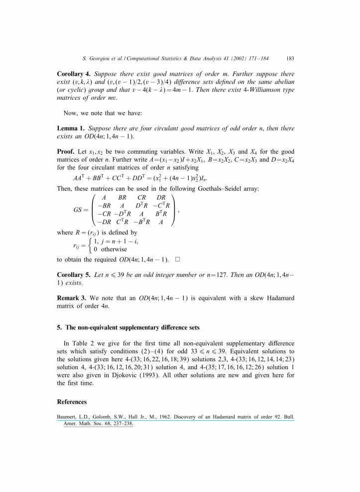
Corollary 4. Suppose there exist good matrices of order m: Further suppose thereexist (v; k; &) and (v; (v − 1)=2; (v − 3)=4) di<erence sets de=ned on the same abelian(or cyclic) group and that v− 4(k − &) = 4m− 1: Then there exist 4-Williamson typematrices of order mv:

Now, we note that we have:

Lemma 1. Suppose there are four circulant good matrices of odd order n; then thereexists an OD(4n; 1; 4n− 1):

Proof. Let x1; x2 be two commuting variables. Write X1; X2; X3 and X4 for the goodmatrices of order n. Further write A=(x1−x2)I+x2X1; B=x2X2; C=x2X3 and D=x2X4

for the four circulant matrices of order n satisfying

AAT + BBT + CCT + DDT = (x21 + (4n− 1)x2

2)In:

Then; these matrices can be used in the following Goethals–Seidel array:

GS =

A BR CR DR−BR A DTR −CTR−CR −DTR A BTR−DR CTR −BTR A

;

where R= (rij) is de6ned by

rij ={

1; j = n+ 1 − i;0 otherwise

to obtain the required OD(4n; 1; 4n− 1):

Corollary 5. Let n6 39 be an odd integer number or n=127. Then an OD(4n; 1; 4n−1) exists.

Remark 3. We note that an OD(4n; 1; 4n − 1) is equivalent with a skew Hadamardmatrix of order 4n:

5. The non-equivalent supplementary di,erence sets

In Table 2 we give for the 6rst time all non-equivalent supplementary di9erencesets which satisfy conditions (2)–(4) for odd 336 n6 39. Equivalent solutions tothe solutions given here 4-(33; 16; 22; 16; 18; 39) solutions 2,3, 4-(33; 16; 12; 14; 14; 23)solution 4, 4-(33; 16; 12; 16; 20; 31) solution 4, and 4-(35; 17; 16; 16; 12; 26) solution 1were also given in Djokovic (1993). All other solutions are new and given here forthe 6rst time.

References

Baumert, L.D., Golomb, S.W., Hall Jr., M., 1962. Discovery of an Hadamard matrix of order 92. Bull.Amer. Math. Soc. 68, 237–238.

184 S. Georgiou et al. / Computational Statistics & Data Analysis 41 (2002) 171–184

Djokovic, D.Z., 1993. Good matrices of order 33, 35 and 127 exist. J. Combin. Math. Combin. Comput. 14,145–152.

Fedorov, V.V., 1972. Theory of Optimal Experiments. Academic Press, New York.Fletcher, R.J., Gysin, M., Seberry, J., 2001. Application of the discrete Fourier transform, to the search for

generalised Legendre pairs and Hadamard matrices. Australas. J. Combin. 23, 75–86.Geramita, A.V., Seberry, J., 1979. Orthogonal designs: Quadratic forms and Hadamard matrices. Marcel

Dekker, New York, Basel.Geramita, A.V., Geramita, J.M., Seberry Wallis, J., 1976. Orthogonal designs. Linear and Multilinear Algebra

3, 281–306.Kounias, S., Chadjipantelis, T., 1983. Some D-optimal weighing designs for n ≡ 3 (mod 4). J. Statist. Plann.

Inference 8, 117–127.Plackett, R.L., Burman, J.P., 1946. The design of optimum multifactorial experiments. Biometrika 33, 305–

325.Press, W.H., Fannery, B.P., Teukolsky, S.A., Vettering, W.T., 1981. Numerical Recipes in Pascal: The Art

of Scienti6c Computing. Cambridge University Press, New York.Seberry Wallis, J., 1972. Hadamard matrices, Part IV, Combinatorics: Room Squares, Sum free sets

and Hadamard matrices. In: Wallis, W.D., Street, A.P., Seberry Wallis, J. (Eds.),, Lecture Notes inMathematics, Vol. 292. Springer, Berlin, Heidelberg, New York.

Seberry Wallis, J., 1975. Construction of Williamson type matrices. Linear and Multilinear Algebra 3, 197–207.

Seberry Wallis, J., 1975. On Hadamard matrices. J. Combin. Theory Ser. A 18, 149–164.Seberry, J., Yamada, M., 1992. Hadamard matrices, sequences and block designs. In: Dinitz, J.H., Stinson,

D.R. (Eds.), Contemporary Design Theory—a Collection of Surveys. Wiley, New York, pp. 431–560.Szekeres, G., 1988. A note on skew type orthogonal ±1 matrices. in: Hajnal, A., Lovasz, L., Sos, V.T. (Eds.),

Combinatorics, Colloquia Mathematica Societatis, Janos Bolyai, No. 52. North-Holland, Amsterdam, pp.489–498.

Tretter, S.A., 1976. Introduction to Discrete—Time Signal Processing. Wiley, New York.Wynn, H.P., 1970. The sequential generation of D-optimal experimental designs. Ann. Math. Statist. 41,

1655–1664.