SIAM J. SCI. COMPUT. c© 2005 Society for Industrial and Applied MathematicsVol. 27, No. 1, pp. 278–293

COMPUTATION OF THE EXPONENTIAL OF LARGE SPARSESKEW-SYMMETRIC MATRICES∗

N. DEL BUONO† , L. LOPEZ† , AND R. PELUSO‡

Abstract. In this paper we consider methods for evaluating both exp(A) and exp(τA)q1 whereexp(·) is the exponential function, A is a sparse skew-symmetric matrix of large dimension, q1 isa given vector, and τ is a scaling factor. The proposed method is based on two main steps: A isfactorized into its tridiagonal form H by the well-known Lanczos iterative process, and then exp(A)is derived making use of an effective Schur decomposition of H. The procedure takes full advantageof the sparsity of A and of the decay behavior of exp(H). Several applications and numerical testsare also reported.

Key words. skew-symmetric matrices, singular value decomposition, geometric integration ofordinary differential equations, splitting techniques

AMS subject classifications. 65F, 65L

DOI. 10.1137/030600758

1. Introduction. Exponential methods for the geometric integration of ordinarydifferential equations (ODEs) with quadratic invariants [13, 17] or for the solution ofpartial differential equations (PDEs) of advection type [4, 7, 16, 26] require comput-ing the exponentials of skew-symmetric matrices as well as preserving the orthogonalfeature of the obtained matrices. Hence, methods for evaluating both exp(A) andexp(τA)q1, where A is a real sparse skew-symmetric matrix of large dimension n, q1is a given vector of Euclidean norm 1, and τ is a scaling factor associable with the stepsize in a time integration method for ODEs, are of particular interest. Exact formulasfor the computation of the exponential of a low dimension skew-symmetric matrix Aare known [1, 21, 24], but unfortunately these are not practical when the dimension nof the matrix A increases. Standard techniques based on Pade and Chebyshev rationalapproximants can be used, but generally they do not preserve exp(τA) on the orthog-onal group except for the diagonal Pade approximants [5]. Polynomial approximants,instead, are based on the approximation of exp(τA)q1 on some Krylov subspace ofdimension m < n, but these techniques are computationally competitive only when mis small compared with n [11, 14, 25]. Furthermore, when A is skew-symmetric withuniformly distributed eigenvalues, no substantial error reduction occurs for m ≤ ‖τA‖as observed in [14].

In [5, 6, 22] methods based on splitting techniques exploiting the Lie algebrastructure of the orthogonal group have been considered to approximate exp(τA) to agiven order of accuracy with respect to τ . In [19, 28] schemes based on the generalizedpolar decomposition of A and involving a computational cost of κn3 flops, where theconstant κ increases with the order of the approximation, have also been presented.

In this paper we suggest a two-step procedure to compute exp(A): A is firstreduced into a tridiagonal form H using the Lanczos tridiagonalization process, then

∗Received by the editors August 27, 2003; accepted for publication (in revised form) September2, 2004; published electronically September 12, 2005.

http://www.siam.org/journals/sisc/27-1/60075.html†Dipartimento di Matematica, Universita degli Studi di Bari, Via E. Orabona 4, I-70125 Bari,

Italy (delbuono@dm.uniba.it, lopezl@dm.uniba.it).‡Dipartimento di Matematica, Politecnico di Bari, Via Amendola 126/B, I-70126 Bari, Italy

(peluso@poliba.it).

278

EXPONENTIAL OF SKEW-SYMMETRIC MATRICES 279

an effective Schur decomposition of H is obtained via the singular value decomposition(SVD) of a bidiagonal matrix B of half dimension n/2. The SVD of such a matrixmay be computed by efficient methods, for instance the Golub and Kahan algorithm[12] or the accurate differential qd algorithm [9, 10]. In exact arithmetic our procedurepreserves exp(A) in the orthogonal group and its main computational cost is 35/8n3

flops to compute exp(A) and O(n2) flops when evaluating exp(A)q1.The paper is organized as follows. In section 2 we describe the procedure to

derive the Schur decomposition of a tridiagonal, skew-symmetric matrix H, then weshow the decay behavior of the entries of exp(H) proving that such a matrix can beconsidered as banded. Generalization to smooth functions f(z) is also considered. Insection 3 our procedure is numerically compared with MATLAB routines for evalu-ating exponentials. Furthermore, we show some applications in the approximation ofexp(τA)q1 on Krylov subspaces, in the numerical solution of ODEs and finally in thecomputation of exponentials of general matrices by using splitting techniques.

2. Functions of skew-symmetric matrices.

2.1. Schur decompositions of A. Let us consider a real skew-symmetric ma-trix A ∈ R

n×n, a vector q1 ∈ Rn of Euclidean norm 1, the Krylov matrix K(A, q1,m) =

[q1 Aq1 A2q1 · · · Am−1q1] ∈ Rn×m, and the Krylov subspace Km = span{q1, Aq1, . . . ,

Am−1q1}. The following result states the conditions for the existence of a Hessenbergform of A.

Theorem 2.1 (see [12]). Suppose Q = [q1 q2 . . . qn] ∈ Rn×n is an orthogonal

matrix. Then Q�AQ = H is an unreduced Hessenberg matrix if and only if R =Q�K(A, q1, n) is nonsingular and upper triangular.

Thus, when K(A, q1, n) is of full rank n, from the QR factorization of K(A, q1, n),it follows that an unreduced Hessenberg form H of A exists. The Hessenberg decom-position, A = QHQ�, is essentially unique when the first column q1 of Q is fixedand its unreduced Hessenberg form H is skew-symmetric and possesses the followingtridiagonal structure:

H =

⎛⎜⎜⎜⎜⎜⎜⎜⎝

0 −h2 0 . . . 0h2 0 −h3 . . . 0. . .. . .. . .0 . . . . . . . . . −hn

0 . . . . . . hn 0

⎞⎟⎟⎟⎟⎟⎟⎟⎠

.(2.1)

For skew-symmetric matrices the reduction to the above tridiagonal form can beperformed using the following Lanczos tridiagonalization process:

Let q1 be a vector of Rn with ‖q1‖ = 1 and set h1 = 0 and q0 = 0.

For j = 1 : nwj = Aqj + hjqj−1;hj+1 = ‖wj‖;qj+1 = wj/hj+1;

endWe have to notice that, in exact arithmetic, the above algorithm is equivalent to theArnoldi process applied to skew-symmetric matrices. It provides an orthogonal matrixQ = [q1 q2 . . . qn] ∈ R

n×n such that Q�AQ = H where H is the tridiagonal matrix in(2.1). Moreover, it allows one to take full advantage of the possible sparsity of A due to

280 N. DEL BUONO, L. LOPEZ, AND R. PELUSO

the matrix-vector products involved. However, in floating-point arithmetic the vectorsqj could progressively lose their orthogonality, in this case, the application of a re-orthogonalization procedure is required [12, 25]. On the contrary, the Arnoldi processpreserves better the orthogonality of the matrix Q, but the tridiagonal structure ofH could be lost into a Hessenberg one. In the numerical tests we implemented theabove tridiagonalization process with a full re-orthogonalization based on the modifiedGram–Schmidt algorithm [8, 23].

For very large size problems, the storage requirement for the vectors qi’s, providingthe similarity transformation of exp(A), becomes the main drawback of the process.In this case the Lanczos procedure has to be modified applying a storage technique: asimple way to overcome this problem consists in running twice the process; after thefirst run the vector c = exp(H)e1 is computed storing only the sequence q1, . . . , qr withr < n depending on the actual available computer memory [3]. Then the second stepconsists in restarting the process from qr to qn without storing them, and evaluatingexp(A)q1 =

∑ni=1 ciqi, where ci is the ith entry of the vector c. Of course, in this

version of the algorithm, the cost may increase up to two times the one of a singlerun, although in the second run the computation of the matrix H can be avoided.

Then, using A = QHQ�, it follows that exp(A) = Q exp(H)Q� and exp(A)q1 =Q exp(H)e1, where e1 is the first vector of the canonical basis of R

n. In this context,the computational problem to deal with is the evaluation of exp(H), which we willtackle adopting a known Schur decomposition of a tridiagonal skew-symmetric matrixH (see Problem 8.6.6 in [12]).

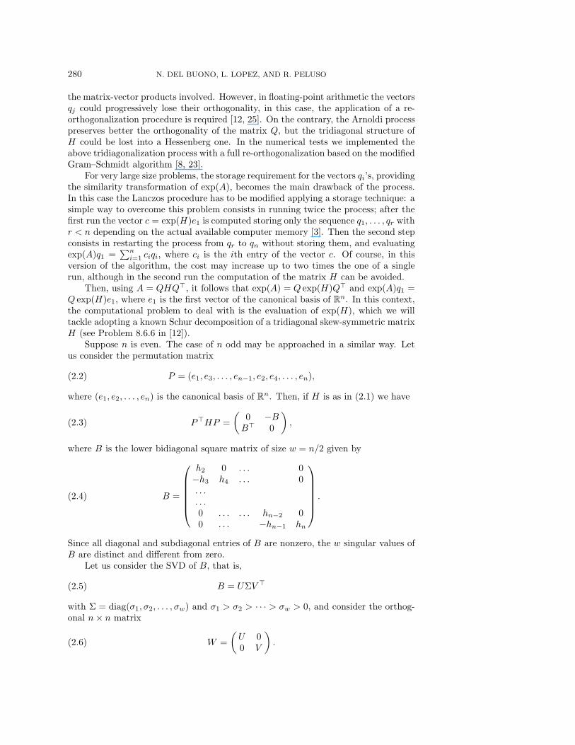
Suppose n is even. The case of n odd may be approached in a similar way. Letus consider the permutation matrix

P = (e1, e3, . . . , en−1, e2, e4, . . . , en),(2.2)

where (e1, e2, . . . , en) is the canonical basis of Rn. Then, if H is as in (2.1) we have

P�HP =

(0 −BB� 0

),(2.3)

where B is the lower bidiagonal square matrix of size w = n/2 given by

B =

⎛⎜⎜⎜⎜⎜⎝

h2 0 . . . 0−h3 h4 . . . 0. . .. . .0 . . . . . . hn−2 00 . . . −hn−1 hn

⎞⎟⎟⎟⎟⎟⎠

.(2.4)

Since all diagonal and subdiagonal entries of B are nonzero, the w singular values ofB are distinct and different from zero.

Let us consider the SVD of B, that is,

B = UΣV �(2.5)

with Σ = diag(σ1, σ2, . . . , σw) and σ1 > σ2 > · · · > σw > 0, and consider the orthog-onal n× n matrix

W =

(U 00 V

).(2.6)

EXPONENTIAL OF SKEW-SYMMETRIC MATRICES 281

Then

W�P�HPW =

(U� 00 V �

)(0 −BB� 0

)(U 00 V

)=

(0 −ΣΣ 0

).

By considering the orthogonal matrix R = PWP� it follows that

P

(0 −ΣΣ 0

)P� = R�HR = diag(S1, S2, . . . , Sw),(2.7)

where

Sj =

(0 −σj

σj 0

)for j = 1, 2, . . . , w(2.8)

is a 2×2 skew-symmetric matrix with eigenvalues given by the pair of pure imaginaryvalues λj,1 = ıσj and λj,2 = −ıσj for j = 1, 2, . . . , w, where ı denotes the imaginaryunit. Thus R provides the real Schur decomposition of H, that is,

H = R diag(S1, S2, . . . , Sw)R�.(2.9)

Finally, the exponential exp(H) may be computed as

exp(H) = R diag(exp(S1), exp(S2), . . . , exp(Sw)) R�,

where

exp(Sj) =

(cosσj − sinσj

sinσj cosσj

)for j = 1, 2, . . . , w.

We can avoid computing R to form exp(H). In fact, from (2.7) and the definition ofR = PWP� it follows that

exp(H) = PW exp

((0 −ΣΣ 0

))W�P�

= PWP�diag(exp(S1), exp(S2), . . . , exp(Sw))PW�P�

= PW

(cos(Σ) − sin(Σ)sin(Σ) cos(Σ)

)W�P�,

where

cos(Σ) = diag(cosσ1, cosσ2, . . . , cosσw),(2.10)

sin(Σ) = diag(sinσ1, sinσ2, . . . , sinσw).(2.11)

Finally,

exp(A) = QPT (U, V,Σ)P�Q�,(2.12)

where T (U, V,Σ) is the following block matrix:

T (U, V,Σ) =

(U cos(Σ)U� −U sin(Σ)V �

V sin(Σ)U� V cos(Σ)V �

).(2.13)

282 N. DEL BUONO, L. LOPEZ, AND R. PELUSO

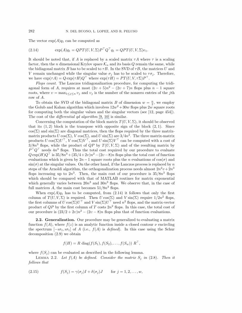
The vector exp(A)q1 can be computed as

exp(A)q1 = QPT (U, V,Σ)P�Q�q1 = QPT (U, V,Σ)e1.(2.14)

It should be noted that, if A is replaced by a scaled matrix τA where τ is a scalingfactor, then the n dimensional Krylov space Kn and its basis Q remain the same, whilethe bidiagonal matrix B has to be scaled to τB. In the SVD of τB, the matrices U andV remain unchanged while the singular value σj has to be scaled to τσj . Therefore,we have exp(τA) = Q exp(τH)Q� where exp(τH) = PT (U, V, τΣ)P�.

Flops count. The Lanczos tridiagonalization procedure, for computing the tridi-agonal form of A, requires at most (2υ + 5)n2 − (2υ + 7)n flops plus n − 1 squareroots, where υ = max1≤j≤n υj and υj is the number of the nonzero entries of the jthrow of A.

To obtain the SVD of the bidiagonal matrix B of dimension w = n2 , we employ

the Golub and Kahan algorithm which involves 12w2 +30w flops plus 2w square rootsfor computing both the singular values and the singular vectors (see [12, page 454]).The cost of the differential qd algorithm [9, 10] is similar.

Concerning the computation of the block matrix T (U, V,Σ), it should be observedthat its (1, 2) block is the transpose with opposite sign of the block (2, 1). Sincecos(Σ) and sin(Σ) are diagonal matrices, then the flops required by the three matrix-matrix products U cos(Σ), V cos(Σ), and U sin(Σ) are 3/4n2. The three matrix-matrixproducts U cos(Σ)U�, V cos(Σ)V �, and U sin(Σ)V � can be computed with a cost of3/8n3 flops, while the product of QP by T (U, V,Σ) and of the resulting matrix byP�Q� needs 4n3 flops. Thus the total cost required by our procedure to evaluateQ exp(H)Q� is 35/8n3 +(35/4+2υ)n2−(2υ−8)n flops plus the total cost of functionevaluations which is given by 2n− 1 square roots plus the n evaluations of cos(σ) andsin(σ) at the singular values. On the other hand, if the Lanczos process is replaced by nsteps of the Arnoldi algorithm, the orthogonalization process needs almost 2n2v+2n3

flops increasing up to 2n3. Then, the main cost of our procedure is 35/8n3 flopswhich should be compared with that of MATLAB routines for matrix exponentialwhich generally varies between 20n3 and 30n3 flops. We observe that, in the case offull matrices A, the main cost becomes 51/8n3 flops.

When exp(A)q1 has to be computed, from (2.14) it follows that only the firstcolumn of T (U, V,Σ) is required. Then U cos(Σ) and V sin(Σ) require 1/2n2 flops,the first columns of U cos(Σ)U� and V sin(Σ)U� need n2 flops, and the matrix-vectorproduct of QP by the first column of T costs 2n2 flops. In this case, the total cost ofour procedure is (23/2 + 2υ)n2 − (2υ − 8)n flops plus that of function evaluations.

2.2. Generalization. Our procedure may be generalized to evaluating a matrixfunction f(A), where f(z) is an analytic function inside a closed contour ν encirclingthe spectrum [−ıσ1, ıσ1] of A (i.e., f(A) is defined). In this case using the Schurdecomposition (2.9) we obtain

f(H) = R diag(f(S1), f(S2), . . . , f(Sw)) R�,

where f(Sj) can be evaluated as described in the following lemma.

Lemma 2.2. Let f(A) be defined. Consider the matrix Sj in (2.8). Then itfollows that

f(Sj) = γ(σj)I + δ(σj)J for j = 1, 2, . . . , w,(2.15)

EXPONENTIAL OF SKEW-SYMMETRIC MATRICES 283

where J = (01−10 ) and where γ(σ), δ(σ) are the following functions on R:

γ(σ) =1

2(f(ıσ) + f(−ıσ)), δ(σ) =

1

2ı(f(ıσ) − f(−ıσ)), σ ∈ R.(2.16)

Moreover, if f(z) is such that f(z) = f(z) for z ∈ C, then γ(σ) and δ(σ) in (2.16)become real infinitely differentiable functions.

Proof. Since Sj has eigenvalues given by λj,1 = ıσj and λj,2 = −ıσj , fromSylvester’s formula [15] we have

f(Sj) =1

λj,1 − λj,2[(f(λj,1) − f(λj,2))Sj + (λj,1f(λj,2) − λj,2f(λj,1))I]

=1

2ı[ı(f(ıσj) + f(−ıσj))I + (f(ıσj) − f(ıσj))J ],

where we have used Sj = σjJ . Thus (2.15) follows. Now, since ıσ = −ıσ, when f(z)

is an analytic function such that f(z) = f(z) for z ∈ C, then it follows that γ(σ) andδ(σ) are real infinitely differentiable functions.

Complex functions f(z) satisfying the condition f(z) = f(z) are cos z; sin z;ϕ(z) = (exp(z) − 1)/z; cay(z) = (1 + z/2)/(1 − z/2) for z �= 2; f(z) = (α + z)−1,with α ≥ 0 and z �= −α. When f(z) = ϕ(z) for all z ∈ C, we have

γ(σ) =sinσ

σ, δ(σ) =

1 − cosσ

σ, σ ∈ R.

When f(z) = cay(z) for all complex values z �= 2, we have

γ(σ) =1 − (σ2 )2

1 + (σ2 )2, δ(σ) =

σ

1 + (σ2 )2, σ ∈ R.

When f(z) = (α + z)−1, with α ≥ 0 and for all complex values z �= −α, we have

γ(σ) =α

α2 + σ2, δ(σ) = − σ

α2 + σ2, σ ∈ R.

The previous results may be summarized in the following theorem.Theorem 2.3. Suppose that n is even. Let A be a real n × n skew-symmetric

matrix and q1 be a vector of Euclidean unit norm such that rank[K(A, q1, n)] = n. LetA = QHQ� be the tridiagonal decomposition of A and suppose that f(A) is defined.Let UΣV � be the SVD of the bidiagonal matrix B in (2.4). Then it follows thatf(A) = Qf(H)Q�, where

f(H) = P

(U Γ(Σ) U� −U Δ(Σ) V �

V Δ(Σ) U� V Γ(Σ) V �

)P�,

where Γ(Σ) and Δ(Σ) are the diagonal matrices

Γ(Σ) = diag(γ(σ1), γ(σ2), . . . , γ(σw)), Δ(Σ) = diag(δ(σ1), δ(σ2), . . . , δ(σw)),(2.17)with γ(σ) and δ(σ) given by (2.16).

284 N. DEL BUONO, L. LOPEZ, AND R. PELUSO

2.3. Decay behavior. Although exp(A) is formally a dense matrix, one cantake computational advantage of the possible decay of its entries away from the maindiagonal. This kind of behavior has been observed in [2] for symmetric positive definitematrices and in [18] for banded matrices. Here, using the SVD of the matrix B, wewill prove that for tridiagonal and skew-symmetric matrices H, the entries of eachblock in T (U, V,Σ) show a decay away from the diagonals. This behavior may beexploited in constructing a banded approximation of T (U, V,Σ).

In order to estimate the size of the entries of T (U, V,Σ), we derive bounds for theinterpolation errors of the functions cosσ and sinσ. Let s be an integer greater than1 and let ξ1, . . . , ξs+1 be the roots of the Chebyshev polynomial τs+1(σ) of degrees + 1 in [σ2

w, σ21 ]. Set γi =

√ξi for i = 1, . . . , s + 1, and consider the interpolation

polynomial p(σ) of cosσ at ±γi for i = 1, . . . , s+1. Since cosσ is an even function, itis easy to see that p(σ) is an even polynomial of degree 2s, i.e., p2s(σ) =

∑sr=0 crσ

2r.Then, cosσ = p2s(σ) + R(σ), with the error function bounded by

|R(σ)| ≤

∣∣∣∏s+1i=1 (σ2 − γ2

i )∣∣∣

(2s + 2)!for σ ∈ R.

Since for i = 1, . . . , s + 1, γ2i = ξi are the roots of τs+1(σ), when σw ≤ σ ≤ σ1 it

follows that ∣∣∣∣∣s+1∏i=1

(σ2 − γ2i )

∣∣∣∣∣ ≤(σ2

1 − σ2w

2

)s+11

2s.

Hence we have

|R(σ)| ≤ (σ21 − σ2

w)s+1

22s+1(2s + 2)!for σw ≤ σ ≤ σ1.(2.18)

Consider the odd function sinσ and the interpolation polynomial at nodes ±γi fori = 1, . . . , s + 1. This polynomial is an odd polynomial of degree 2s + 1, i.e., sinσ =p2s+1(σ) + R(σ), where p2s+1(σ) =

∑sr=0 drσ

2r+1 and

|R(σ)| ≤

∣∣∣∏s+1i=1 (σ2 − γ2

i )∣∣∣

(2s + 2)!for σ ∈ R,

therefore it follows that

|R(σ)| ≤ (σ21 − σ2

w)s+1

22s+1(2s + 2)!for σw ≤ σ ≤ σ1.(2.19)

Theorem 2.4. Let B = UΣV � be the SVD of the bidiagonal matrix B in (2.4)and let cos(Σ) and sin(Σ) be the diagonal matrices in (2.10), (2.11). Then, for eachinteger s ≥ 1, the following bounds of the entries of each block of the matrix T (U, V,Σ)in (2.12) follow:

|[U cos(Σ)U�]k,l| ≤ u(s, σ1, σw) for |k − l| ≥ s + 1,(2.20)

|[V cos(Σ)V �]k,l| ≤ u(s, σ1, σw) for |k − l| ≥ s + 1,(2.21)

|[U sin(Σ)V �]k,l| ≤ u(s, σ1, σw) for |k − l| ≥ s + 1, k − l �= s + 1,(2.22)

EXPONENTIAL OF SKEW-SYMMETRIC MATRICES 285

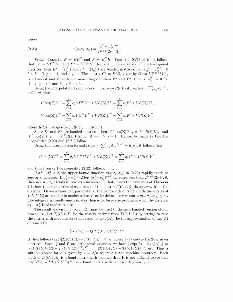
where

u(s, σ1, σw) =(σ2

1 − σ2w)s+1

22s+1(2s + 2)!.(2.23)

Proof. Consider E = BB� and F = B�B. From the SVD of B, it followsthat Es = UΣ2sU� and F s = V Σ2sV � for s ≥ 1. Since E and F are tridiagonal

matrices, then Es = (e(s)kl ) and F s = (f

(s)kl ) are banded matrices, i.e., e

(s)kl = f

(s)kl = 0

for |k − l| ≥ s + 1, and s ≥ 1. The matrix Gs = EsB, given by Gs = UΣ2s+1V �,

is a banded matrix with one more diagonal than Es and F s, that is, g(s)kl = 0 for

|k − l| ≥ s + 1 and k − l �= s + 1.Using the interpolation formula cosσ = p2s(σ)+R(σ) with p2s(σ) =

∑sr=0 crσ

2r,it follows that

U cos(Σ)U� =

s∑r=0

crUΣ2rU� + UR(Σ)U� =

s∑r=0

crEr + UR(Σ)U�,

V cos(Σ)V � =

s∑r=0

crV Σ2rV � + V R(Σ)V � =

s∑r=0

crFr + V R(Σ)V �,

where R(Σ) = diag(R(σ1), R(σ2), . . . , R(σw)).Since Es and F s are banded matrices, then [U� cos(Σ)U ]kl = [U�R(Σ)U ]kl and

[V � cos(Σ)V ]kl = [V �R(Σ)V ]kl for |k − l| ≥ s + 1. Hence, by using (2.18), theinequalities (2.20) and (2.21) follow.

Using the interpolation formula sinσ =∑s

r=0 drσ2r+1 + R(σ), it follows that

U sin(Σ)V � =

s∑r=0

drUΣ2r+1V � + UR(Σ)V � =

s∑r=0

drGr + UR(Σ)V �,

and thus from (2.19), inequality (2.22) follows.If σ2

1 − σ2w < 2, the upper bound function u(s, σ1, σw) in (2.23) rapidly tends to

zero as s increases. If σ21 −σ2

w ≥ 2 but (σ21 −σ2

w)s+1 increases, less than 22s+1(2s+2)!,then u(s, σ1, σw) tends to zero as s increases. In both cases the estimates of Theorem2.4 show that the entries of each block of the matrix T (U, V,Σ) decay away from thediagonal. Given a threshold parameter ε, the bandwidth outside which the entries ofT (U, V,Σ) are smaller in modulus than ε can be defined as r = min{s|u(s, σ1, σw) ≤ ε}.The integer r is usually much smaller than w for large size problems, when the distanceσ2

1 − σ2w is of moderate size.

The result shown in Theorem 2.4 may be used to define a banded version of ourprocedure. Let Tε(U, V,Σ) be the matrix derived from T (U, V,Σ) by setting to zerothe entries with modulus less than ε and let [exp(A)]ε be the approximation of exp(A)obtained by

[exp(A)]ε = QPTε(U, V,Σ)Q�P�.

It then follows that ‖Tε(U, V,Σ)−T (U, V,Σ)‖ ≤ nε, where ‖ ·‖ denotes the 2-norm onmatrices. Since Q and P are orthogonal matrices, we have ‖ exp(A) − [exp(A)]ε‖ =‖QP [T (U, V,Σ) − Tε(U, V,Σ)]Q�P�‖ = ‖Tε(U, V,Σ) − T (U, V,Σ)‖ ≤ nε. Thus asuitable choice for ε is given by ε = ε/n where ε is the machine accuracy. Eachblock of Tε(U, V,Σ) is a band matrix with bandwidth r. It is not difficult to see that[exp(H)]ε = PTε(U, V,Σ)P� is a band matrix with bandwidth given by 2r.

286 N. DEL BUONO, L. LOPEZ, AND R. PELUSO

Flops count in the banded case. Since each block of Tε(U, V,Σ) is a banded matrixof bandwidth r, the two matrix-matrix products in U cos(Σ)U� and V cos(Σ)V �

require 2w(2w− r)(r+1) flops, while the matrix-matrix product in U sin(Σ)V � costs2w2 +2w[2(w−1)−r](r+1) flops, with w = n

2 . The matrix-matrix product of QP byTε(U, V,Σ) can be performed with a cost of 4n2(2r+1) flops. Recalling that w = n/2and that υ is the (maximum by rows) number of nonzero entries, the total cost of ourprocedure is 2n3 +(2υ+61/4+10r)n2− (2υ+2r2 +4r+8)n plus the cost of functionevaluations.

As before, if the vector exp(A)q1 only has to be computed, we need 4w(2r+1) flopsto compute the first column vectors of U cos(Σ)U� and V sin(Σ)V �, while 4n(2r+1)are the flops required for the matrix-vector product of QP by the first column ofT (U, V,Σ). Thus, our procedure now requires (17/2 + 2υ)n2 − (2υ − 12r)n plus thecost of function evaluations. The partial costs are not reported since they equal theones of the nonbanded case (refer to the end of section 2.1).

3. Applications and numerical tests. All numerical tests have been obtainedrunning MATLAB 5.3 on a Pentium IV 2.4 GHz with 1024 MbRAM. In the numericalcodes we have implemented the Lanczos tridiagonalization process with a full re-orthogonalization based on the iterated modified Gram–Schmidt algorithm [8, 23];the SVD of the bidiagonal matrix B has been performed exploiting the Golub andKahan algorithm. Moreover, no storage techniques has been adopted.

The procedure for computing exp(A) by (2.12) has been denoted by AExp, whileAbExp(r) denotes the procedure in which T (U, V,Σ) is replaced by Tε(U, V,Σ), wherethe bandwidth r of each block of Tε(U, V,Σ) is given by min{s|u(s, σ1, σw) ≤ ε}, withε = ε/n and ε = 2.2206e − 16 (the MATLAB floating point relative accuracy).

3.1. Numerical comparisons. We have compared our approaches with twoMATLAB functions Expm and Expm3. Particularly, Expm computes the exponentialof A using a scaling and squaring algorithm with Pade approximations, while Expm3

evaluates the exponential of A via eigenvalue and eigenvector decomposition. Com-parisons are done in terms of: Flops (counted by the built in MATLAB routineflops); global error, defined as the 2-norm of the difference of AExp (respectively,AbExp) and Expm; orthogonal error, defined as the distance of the computed expo-nential from the orthogonal manifold (i.e., ‖AExp�AExp − In‖F , where ‖ · ‖F is theFrobenius norm on matrices). Tables 3.1 and 3.2 report the comparisons on sparseand dense skew-symmetric matrices A of different dimensions n and entries randomlygenerated in [−10, 10]. Observe that the results obtained for AExp and AbExp(r) aresimilar, nevertheless AbExp(r) saves flops.

3.2. Krylov approximations of exp(τA)q1. When we need to compute y =exp(τA)q1 and n is large, the tridiagonalization process to obtain H may be tooexpensive. In this case a common way to save computation is to consider the approx-imation, ym = Qm exp(τHm)e1, on the Krylov subspace of dimension m < n, wheree1 = (1, 0, . . . , 0)� ∈ R

m, and Qm, Hm are the matrices derived by the Krylov algo-rithm that is the Lanczos tridiagonalization process in section 2.1 run until m < n.However, when A is a skew-symmetric matrix with uniformly distributed eigenval-ues, no substantial error reduction can be observed for m ≤ ‖τA‖ ([14]), and thusthe Krylov algorithm should be implemented in a different way than for symmetricmatrices. In particular, we fix m sufficiently large and consider the approximationym = Qm exp(τHm)e1 then an a posteriori error estimate has to be used to evaluatethe Krylov approximation obtained.

EXPONENTIAL OF SKEW-SYMMETRIC MATRICES 287

Table 3.1

Comparisons on sparse matrices.

n Method Flops Global error Orthogonal errorAExp 1145932 9.0129e-15 1.5095e-14

50 AbExp(9) 1106808 2.9155e-14 7.9203e-14Expm 2664508 - 1.3323e-15Expm3 5231760 - 2.2204e-16AExp 8791319 2.9465e-14 3.7254e-14

100 AbExp(11) 8328146 2.9737e-14 3.5312e-14Expm 22990654 - -3.7748e-15Expm3 40867683 - 1.3323e-15AExp 68324797 5.4209e-14 8.2757e-14

200 AbExp(13) 63746408 5.4535e-14 7.4573e-14Expm 182624884 - 8.6597e-15Expm3 318490737 - 8.8818e-16AExp 9595372489 1.8063e-11 5.5681e-13

1000 AbExp(57) 9095990316 1.8867e-11 5.5681e-13Expm 38696969972 - 8.9447e-11Expm3 38702914947 - 3.3599e-12

Table 3.2

Comparisons on dense matrices.

n Method Flops Global error Orthogonal errorAExp 1372571 7.6373e-14 1.8952e-14

50 AbExp(18) 1367152 7.6353e-14 1.9060e-14Expm 2664508 - 1.3323e-15Expm3 5231760 - 2.2204e-16AExp 10576419 7.1397e-14 3.3902e-14

100 AbExp(21) 10322746 7.1459e-14 3.5483e-14Expm 26989568 - 5.5511e-15Expm3 40807089 - 8.8818e-16AExp 82521976 2.7667e-13 1.0002e-13

200 AbExp(27) 79302399 2.7657e-13 1.1354e-13Expm 230628400 - 1.7319e-14Expm3 318630721 - 8.8818e-16AExp 10084256626 2.2523e-12 6.6374e-13

1000 AbExp(36) 9430845640 2.0543e-12 8.9980e-13Expm 32696962184 - 3.4766e-11Expm3 38733904231 - 3.0348e-12

AExpy denotes the method based on formula (2.14) for evaluating y = exp(τA)q1while KExpy(m) indicates the Krylov approximation, ym = Qm exp(τHm)e1, whereQm and exp(τHm) are computed by our procedure, while KExpmy(m) marks the Krylovapproximation where the exponential exp(τHm) is computed using the MATLABfunction Expm. In Table 3.3 we compare the results obtained by AExpy, KExpy(m), andKExpmy(m), where A is a dense random matrix with entries in [−1, 1] and q1 a vector ofEuclidean unit norm. The results show that KExpy(m) always saves computation withrespect to AExpy and KExpmy(m). We have also applied our procedure to computethe vector y = exp(A)q1, where A is now a 300 × 300 sparse skew-symmetric matrix,with about 10% nonzero elements randomly generated in [−10, 10], and q1 is a randomvector with ‖q1‖ = 1. Figure 3.1 shows the semilog plot of the global error (dotted linewith circle) evaluated as ‖y−ym‖, and of the orthogonal error, defined as |y�mym−1|,(solid line with stars), against the dimension m of the Krylov subspace. Figure 3.1shows that accurate Krylov approximations may be obtained for quite large values ofm.

288 N. DEL BUONO, L. LOPEZ, AND R. PELUSO

Table 3.3

Comparisons for computing exp(A)q.

n Method Flops Global error Orthogonal error100 AExpy 5843843 2.8015e-14 4.4409e-16

KExpy(25) 663918 2.8398e-14 4.4409e-16KExpmy(25) 955870 2.7832e-14 2.8866e-15

200 AExpy 44591067 8.4962e-14 1.1102e-16KExpy(50) 5319882 8.1275e-14 4.4409e-16KExpmy(50) 7784495 8.1730e-14 1.1102e-15

300 AExpy 148907702 6.9981e-14 8.8818e-16KExpy(70) 16314427 6.2032e-14 3.1086e-15KExpmy(70) 22392695 6.1764e-14 2.2204e-16

0 50 100 150 200 250 30010

–16

10– 14

10– 12

10– 10

10– 8

10– 6

10– 4

10– 2

100

102

m

Fig. 3.1. Errors behavior.

3.3. Application to ODEs and PDEs. We consider the method of Magnusseries, which approximates the solution of linear differential equations y′ = A(t)y,y(0) = y0 in the form y(t) = exp(Ω(t))y0, where Ω(t) is a matrix function satisfying asuitable ODE [13, 17]. When A(t) is a skew-symmetric matrix function, Ω(t) is alsoskew-symmetric and y(t) is a vector with ‖y(t)‖ = 1 for all t. We adopt our approachto compute the exponentials of the second and fourth order Magnus methods, whosedefinitions are reported below (h is the time step):

MG2 MG4

A1 = A(tn + h/2); A1 = A(tn + ( 12 −

√3

6 )h);

ωn = A1; A2 = A(tn + ( 12 +

√3

6 )h);

yn+1 = exp(hωn)yn; ωn = 12 (A1 + A2) +

√3

12 h[A2, A1];yn+1 = exp(hωn)yn.

As an example we consider the skew-symmetric matrix A(t) = (aij(t)), whose uppertriangular entries are aij(t) = (−1)i+j i

j+1 tj−i, 1 ≤ i < j ≤ n [20]. In the com-

putation we have taken n = 100 and we integrate the differential system y′ = A(t)yon the interval [0, 1]; as initial vector a vector y(0) randomly generated and withunit Euclidean norm has been employed . Denote by ZpExp the method of order p,with respect to the time step h, proposed in [28]. It preserves exponential matriceson the orthogonal group and its cost is of κn3 flops, where the constant κ increaseswith the order p of the approximation. MGp(AExpy) and MGp(ZpExp) denote the

EXPONENTIAL OF SKEW-SYMMETRIC MATRICES 289

Magnus methods in which the exponential matrices, at each step, are computed byAExpy and ZpExp, respectively. Table 3.4 reports the performance of the methods.It can be seen that MGp(ZpExpy) are less accurate than MGp(AExpy). However thesecond order Magnus method based on Z2Exp saves flops with respect to MG2(AExpy)although this favorable feature is less clear when we compare fourth order methodsMG4(Z4Exp) and MG4(AExpy), since ZpExp have a cost increasing with the order pof the approximation. The schemes MGp(KExpy(m)), based on the approximation ofKrylov subspace, show the same performance in terms of orthogonal and global errorsas MGp(AExpy), while reducing the number of flops required.

Table 3.4

Performance of second and fourth order methods.

h Method Flops Orthogonal error Global errorh = 0.1 MG2(AExpy) 58898468 1.1990e-14 0.0025

MG2(KExpy(10)) 2625917 3.5527e-15 0.0025MG2(Z2Exp) 8281742 4.4409e-16 0.0216MG4(AExpy) 99830866 7.9936e-15 3.3569e-4

MG4(KExpy(10)) 43620601 5.3291e-15 3.3569e-4MG4(Z4Expy) 67318182 5.5511e-16 0.0021

h = 0.05 MG2(AExpy) 117785480 7.7716e-15 7.3285e-4MG2(KExpy(10)) 10500852 7.1054e-15 7.3285e-4MG2(Z2Expy) 16563482 2.2204e-16 0.0079MG4(AExpy) 199697270 1.4433e-14 5.2503e-5

MG4(KExpy(10)) 87240935 6.2172e-15 5.2503e-5MG4(Z4Exp) 134636362 8.8818e-16 2.4964e-4

h = 0.025 MG2(AExpy) 235500110 5.5511e-15 1.9819e-4MG2(KExpy(10)) 10500852 7.1054e-15 1.9819e-4MG2(Z2Expy) 33126962 6.6613e-16 0.0023MG4(AExpy) 399342752 1.7986e-14 4.5198e-6

MG4(KExpy(10)) 174480892 9.3259e-15 4.5198e-6MG4(Z4Exp) 269272722 2.5535e-15 1.8543e-5

We now consider a different example, in particular the KdV PDE ut = −uux −δ2uxxx, with periodic boundary conditions u(0, t) = u(L, t), where L is the period andδ is a small parameter. As shown in [7], appropriate methods of space discretizationlead to solve a set of ODEs of the form y′ = A(y)y, y(0) = y0, evolving on thesphere of radius ‖y0‖, where y(t) = (u0(t), u1(t), . . . , uN−1(t))

�, ui(t) ≈ u(iΔx, t) fori = 0, 1, . . . , N − 1, and where Δx = 2

N is the spatial step of [0, 2]. For instance, if weconsider the space discretization method in [26] we have

A(y) = − 1

6Δxg(y) − δ2

2Δx3P,

where both g(y) and P are two N ×N skew-symmetric matrices given by

g(y) =

⎛⎜⎜⎜⎜⎜⎝

0 u0 + u1 0 0 0 −(u0 + uN−1)−(u0 + u1) 0 u1 + u2 . . . 0 0

0 −(u1 + u2) 0 . . . 0 0...

......

......

uN−1 + u0 0 0 . . . −(uN−1 + uN−2) 0

⎞⎟⎟⎟⎟⎟⎠

290 N. DEL BUONO, L. LOPEZ, AND R. PELUSO

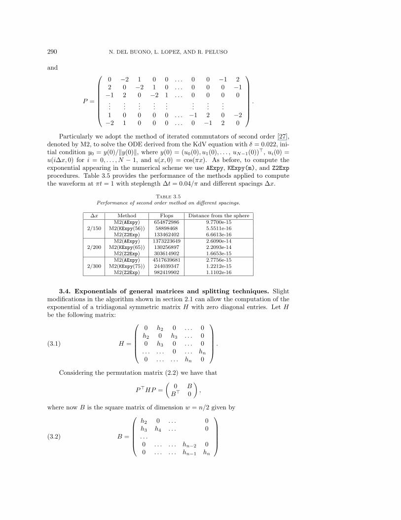
and

P =

⎛⎜⎜⎜⎜⎜⎜⎜⎝

0 −2 1 0 0 . . . 0 0 −1 22 0 −2 1 0 . . . 0 0 0 −1−1 2 0 −2 1 . . . 0 0 0 0...

......

......

......

...1 0 0 0 0 . . . −1 2 0 −2−2 1 0 0 0 . . . 0 −1 2 0

⎞⎟⎟⎟⎟⎟⎟⎟⎠

.

Particularly we adopt the method of iterated commutators of second order [27],denoted by M2, to solve the ODE derived from the KdV equation with δ = 0.022, ini-tial condition y0 = y(0)/‖y(0)‖, where y(0) = (u0(0), u1(0), . . . , uN−1(0))�, ui(0) =u(iΔx, 0) for i = 0, . . . , N − 1, and u(x, 0) = cos(πx). As before, to compute theexponential appearing in the numerical scheme we use AExpy, KExpy(m), and Z2Exp

procedures. Table 3.5 provides the performance of the methods applied to computethe waveform at πt = 1 with steplength Δt = 0.04/π and different spacings Δx.

Table 3.5

Performance of second order method on different spacings.

Δx Method Flops Distance from the sphereM2(AExpy) 654872986 9.7700e-15

2/150 M2(KExpy(56)) 58898468 5.5511e-16M2(Z2Exp) 133462402 6.6613e-16M2(AExpy) 1373223649 2.6090e-14

2/200 M2(KExpy(65)) 130256897 2.2093e-14M2(Z2Exp) 303614902 1.6653e-15M2(AExpy) 4517639681 2.7756e-15

2/300 M2(KExpy(75)) 244039347 1.2212e-15M2(Z2Exp) 982419902 1.1102e-16

3.4. Exponentials of general matrices and splitting techniques. Slightmodifications in the algorithm shown in section 2.1 can allow the computation of theexponential of a tridiagonal symmetric matrix H with zero diagonal entries. Let Hbe the following matrix:

H =

⎛⎜⎜⎜⎜⎝

0 h2 0 . . . 0h2 0 h3 . . . 00 h3 0 . . . 0. . . . . . 0 . . . hn

0 . . . . . . hn 0

⎞⎟⎟⎟⎟⎠ .(3.1)

Considering the permutation matrix (2.2) we have that

P�HP =

(0 BB� 0

),

where now B is the square matrix of dimension w = n/2 given by

B =

⎛⎜⎜⎜⎜⎝

h2 0 . . . 0h3 h4 . . . 0. . .0 . . . . . . hn−2 00 . . . . . . hn−1 hn

⎞⎟⎟⎟⎟⎠(3.2)

EXPONENTIAL OF SKEW-SYMMETRIC MATRICES 291

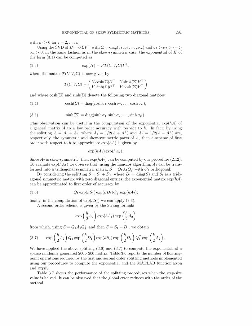
with hi > 0 for i = 2, . . . , n.Using the SVD of B = UΣV � with Σ = diag(σ1, σ2, . . . , σw) and σ1 > σ2 > · · · >

σw > 0, in the same fashion as in the skew-symmetric case, the exponential of H ofthe form (3.1) can be computed as

exp(H) = PT (U, V,Σ)P�,(3.3)

where the matrix T (U, V,Σ) is now given by

T (U, V,Σ) =

(U cosh(Σ)U� U sinh(Σ)V �

V sinh(Σ)U� V cosh(Σ)V �

)

and where cosh(Σ) and sinh(Σ) denote the following two diagonal matrices:

cosh(Σ) = diag(coshσ1, coshσ2, . . . , coshσw),(3.4)

sinh(Σ) = diag(sinhσ1, sinhσ2, . . . , sinhσw).(3.5)

This observation can be useful in the computation of the exponential exp(hA) ofa general matrix A to a low order accuracy with respect to h. In fact, by usingthe splitting A = A1 + A2, where A1 = 1/2(A + A�) and A2 = 1/2(A − A�) are,respectively, the symmetric and skew-symmetric parts of A, then a scheme of firstorder with respect to h to approximate exp(hA) is given by

exp(hA1) exp(hA2).

Since A2 is skew-symmetric, then exp(hA2) can be computed by our procedure (2.12).To evaluate exp(hA1) we observe that, using the Lanczos algorithm, A1 can be trans-formed into a tridiagonal symmetric matrix S = Q1A1Q

�1 with Q1 orthogonal.

By considering the splitting S = S1 + D1, where D1 = diag(S) and S1 is a tridi-agonal symmetric matrix with zero diagonal entries, the exponential matrix exp(hA)can be approximated to first order of accuracy by

Q1 exp(hS1) exp(hD1)Q�1 exp(hA2);(3.6)

finally, in the computation of exp(hS1) we can apply (3.3).A second order scheme is given by the Strang formula

exp

(h

2A2

)exp(hA1) exp

(h

2A2

)

from which, using S = Q1A1Q�1 and then S = S1 + D1, we obtain

exp

(h

2A2

)Q1 exp

(h

2D1

)exp(hS1) exp

(h

2D1

)Q�

1 exp

(h

2A2

).(3.7)

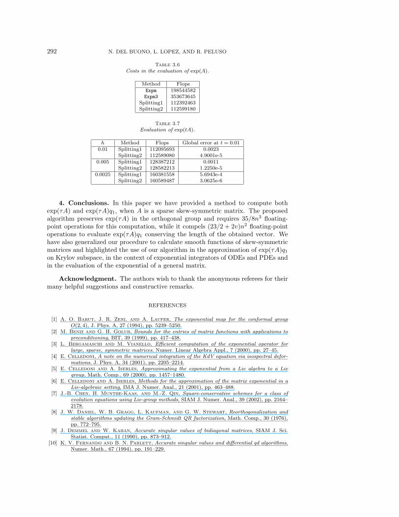
We have applied the above splitting (3.6) and (3.7) to compute the exponential of asparse randomly generated 200×200 matrix. Table 3.6 reports the number of floating-point operations required by the first and second order splitting methods implementedusing our procedures to compute the exponential and the MATLAB function Expm

and Expm3.Table 3.7 shows the performance of the splitting procedures when the step-size

value is halved. It can be observed that the global error reduces with the order of themethod.

292 N. DEL BUONO, L. LOPEZ, AND R. PELUSO

Table 3.6

Costs in the evaluation of exp(A).

Method FlopsExpm 198544582Expm3 353673645

Splitting1 112392463Splitting2 112599180

Table 3.7

Evaluation of exp(tA).

h Method Flops Global error at t = 0.010.01 Splitting1 112095693 0.0023

Splitting2 112589080 4.9001e-50.005 Splitting1 128387212 0.0011

Splitting2 128582213 1.2250e-50.0025 Splitting1 160381558 5.6943e-4

Splitting2 160589487 3.0625e-6

4. Conclusions. In this paper we have provided a method to compute bothexp(τA) and exp(τA)q1, when A is a sparse skew-symmetric matrix. The proposedalgorithm preserves exp(τA) in the orthogonal group and requires 35/8n3 floating-point operations for this computation, while it compels (23/2 + 2v)n2 floating-pointoperations to evaluate exp(τA)q1 conserving the length of the obtained vector. Wehave also generalized our procedure to calculate smooth functions of skew-symmetricmatrices and highlighted the use of our algorithm in the approximation of exp(τA)q1on Krylov subspace, in the context of exponential integrators of ODEs and PDEs andin the evaluation of the exponential of a general matrix.

Acknowledgment. The authors wish to thank the anonymous referees for theirmany helpful suggestions and constructive remarks.

REFERENCES

[1] A. O. Barut, J. R. Zeni, and A. Laufer, The exponential map for the conformal groupO(2, 4), J. Phys. A, 27 (1994), pp. 5239–5250.

[2] M. Benzi and G. H. Golub, Bounds for the entries of matrix functions with applications topreconditioning, BIT, 39 (1999), pp. 417–438.

[3] L. Bergamaschi and M. Vianello, Efficient computation of the exponential operator forlarge, sparse, symmetric matrices, Numer. Linear Algebra Appl., 7 (2000), pp. 27–45.

[4] E. Celledoni, A note on the numerical integration of the KdV equation via isospectral defor-mations, J. Phys. A, 34 (2001), pp. 2205–2214.

[5] E. Celledoni and A. Iserles, Approximating the exponential from a Lie algebra to a Liegroup, Math. Comp., 69 (2000), pp. 1457–1480.

[6] E. Celledoni and A. Iserles, Methods for the approximation of the matrix exponential in aLie-algebraic setting, IMA J. Numer. Anal., 21 (2001), pp. 463–488.

[7] J.-B. Chen, H. Munthe-Kaas, and M.-Z. Qin, Square-conservative schemes for a class ofevolution equations using Lie-group methods, SIAM J. Numer. Anal., 39 (2002), pp. 2164–2178.

[8] J. W. Daniel, W. B. Gragg, L. Kaufman, and G. W. Stewart, Reorthogonalization andstable algorithms updating the Gram-Schmidt QR factorization, Math. Comp., 30 (1976),pp. 772–795.

[9] J. Demmel and W. Kahan, Accurate singular values of bidiagonal matrices, SIAM J. Sci.Statist. Comput., 11 (1990), pp. 873–912.

[10] K. V. Fernando and B. N. Parlett, Accurate singular values and differential qd algorithms,Numer. Math., 67 (1994), pp. 191–229.

EXPONENTIAL OF SKEW-SYMMETRIC MATRICES 293

[11] E. Gallopoulos and Y. Saad, Efficient solution of parabolic equations by Krylov approxima-tion methods, SIAM J. Sci. Statist. Comput., 13 (1992), pp. 1236–1264.

[12] G. H. Golub and C. F. van Loan, Matrix Computation, 3rd ed., The John Hopkins UniversityPress, Baltimore, 1996.

[13] E. Hairer, C. Lubich, and G. Wanner, Geometric Numerical Integration: Structure-Preserving Algorithms for Ordinary Differential Equations, Springer-Verlag, Berlin, 2002.

[14] M. Hochbruck and C. Lubich, On Krylov subspace approximations to the matrix exponentialoperator, SIAM J. Numer. Anal., 34 (1997) pp. 1911–1925.

[15] R. Horn and C. Johnson, Topics in Matrix Analysis, Cambridge University Press, New York,1995.

[16] W. H. Hundsdorfer, Numerical Solution of Advection-Diffusion-Reaction Equations, CWIReport NM-N9603, Center for Mathematics and Computer Science CWI, Amsterdam,1996.

[17] A. Iserles, H. Munthe-Kaas, S. Nørsett, and A. Zanna, Lie-group methods, in Acta Nu-merica, Acta Numer. 9, Cambridge University Press, Cambridge, UK, 2000, pp. 215–365.

[18] A. Iserles, How large is the exponential of a banded matrix?, New Zealand J. Math., 29 (2000),pp. 177–192.

[19] A. Iserles and A. Zanna, Efficient computation of the matrix exponential by generalized polardecompositions, SIAM J. Numer. Anal., 42 (2005), pp. 2218–2256.

[20] A. Iserles, E. Marthinsen, and S. Nørsett, On the implementation of the method of Magnusseries for linear differential equations, BIT, 39 (1999), pp. 281–304.

[21] F. S. Leite and P. Crouch, Closed forms for the exponential mapping on matrix Lie groupsbased on Putzer’s method, J. Math. Phys., 40 (1999), pp. 3561–3568.

[22] B. Leimkuhler, Adaptive geometric integrators based on splitting, scaling, and switching, inInternational Conference on Differential Equations, Vol. 1, 2, World Scientific, River Edge,NJ, 2000, pp. 988–993.

[23] B. N. Parlett, The Symmetric Eigenvalue Problem, Prentice–Hall, Englewood Cliffs, NJ,1980.

[24] T. Politi, A formula for the exponential of a real skew symmetric matrix of order 4, BIT, 41(2001), pp. 842–845.

[25] Y. Saad, Analysis of some Krylov subspace approximations to the matrix exponential operator,SIAM J. Numer. Anal., 29 (1992), pp. 209–228.

[26] N. J. Zabusky and M. D. Kruskal, Interaction of solitons in a collisionless plasma and therecurrence of initial states, Phys. Rev. Lett., 15 (1965), pp. 240–243.

[27] A. Zanna, The Method of Iterated Commutators for Ordinary Differential Equations on LieGroups, DAMTP Technical report NA1996/12, University of Cambridge, Cambridge, UK,1996.

[28] A. Zanna and H. Z. Munthe-Kaas, Generalized polar decompositions for the approximationof the matrix exponential, SIAM J. Matrix Anal. Appl., 23 (2002), pp. 840–862.