Hindawi Publishing CorporationEURASIP Journal on Advances in Signal ProcessingVolume 2008, Article ID 816507, 13 pagesdoi:10.1155/2008/816507

Research ArticleSparse Deconvolution Using Support Vector Machines

Jose Luis Rojo-Alvarez,1 Manel Martınez-Ramon,2 Jordi Munoz-Marı,3 Gustavo Camps-Valls,3

Carlos M. Cruz,2 and Anıbal R. Figueiras-Vidal2

1 Department of Signal Theory and Communications, Universidad Rey Juan Carlos, Camino del Molino s/n,28943 Fuenlabrada, Madrid, Spain

2 Department of Signal Theory and Communications, Universidad Carlos III de Madrid, Avda Universidad,30, 28911 Leganes, Madrid, Spain

3 Departament d’Enginyeria Electronica, Universitat de Valencia, 46010 Valencia, Spain

Correspondence should be addressed to Jose Luis Rojo-Alvarez, joseluis.rojo@urjc.es

Received 26 September 2007; Revised 18 January 2008; Accepted 17 March 2008

Recommended by Theodoros Evgeniou

Sparse deconvolution is a classical subject in digital signal processing, having many practical applications. Support vector machine(SVM) algorithms show a series of characteristics, such as sparse solutions and implicit regularization, which make them attractivefor solving sparse deconvolution problems. Here, a sparse deconvolution algorithm based on the SVM framework for signalprocessing is presented and analyzed, including comparative evaluations of its performance from the points of view of estimationand detection capabilities, and of robustness with respect to non-Gaussian additive noise.

Copyright © 2008 Jose Luis Rojo-Alvarez et al. This is an open access article distributed under the Creative Commons AttributionLicense, which permits unrestricted use, distribution, and reproduction in any medium, provided the original work is properlycited.

1. INTRODUCTION

The sparse deconvolution (SD) problem consists in theestimation of an unknown sparse sequence which has beenconvolved with a (known) time series (impulse responseof the system or source wavelet) and corrupted by noise,producing the observed noisy time series. The nonnull sam-ples of the sparse series contain relevant information aboutthe underlying physical phenomenon in each application.After its first application to reflective seismology [1], SDhas been also used in a number of fields, such as ultrasonicnondestructive evaluation, image restoration, or cancelationof fractionated activity in intracardiac electrograms [2–4].

There has been an intensive development of SD tech-niques and algorithms. Since they are easy to compute, leastsquares (LSs) methods [5] have been used to deconvolvesparse seismic signals [6–9]. Some of the drawbacks ofLS methods are their lack of robustness (they are verysensitive to non-Gaussian noise), and the ill-posing of theproblem when the number of unknowns is close to thenumber of observations. Many complementary methodshave been presented, such as Tikhonov’s regularization [10]

(also known in the statistical literature as ridge regression[11]), total LS [12], covariance shaping LS estimation [13],or signal-adaptive constraints [14]. The L1 loss solutionto SD [7] offers advantage in terms of sparseness whencompared to the L2 loss solution, also known as meansquared error (MSE) criterion technique. L1-penalized SDwas proposed later [15], by including an additional regular-ization term which consists on the L1-norm of the unknownsignal, allowing to control the sparseness of the solution.The Simplex algorithm was introduced as an optimizationmethod for L1-penalized SD in [2]. More recently, large scalelinear programming methods have been also presented [16].

Maximum-likelihood deconvolution (MLD) was firstdeveloped by using state-variable models [17], but a morewidespread used convolutional model was presented in [1],assuming that the sparse signal has a Bernoulli-Gaussian(BG) distribution and that the impulse response can bemodeled as an autoregressive and moving average (ARMA)signal model. The Gaussian mixture (GM) model for SDassumes that the prior distribution of the sparse signal isa mixture of a narrow and a broad Gaussian distributions[18], and the BG distribution is a special case of the GM.Based on an extensive work in robust estimation [13, 19–21],

2 EURASIP Journal on Advances in Signal Processing

a minimax MSE estimation filter that minimizes somemeasure of the worst case pointwise MSE was developed in[22]. In [23], a double postprocessing was applied after aninverse filtering of the observations, which corresponds to aregularization in the Tikhonov sense and a subsequent noiseattenuation.

In general, the performance of SD algorithms can bedegraded by several causes. First, they can result in numer-ically ill-posed problems [18], and regularization methodsare often required. Also when the knowledge about the noiseis limited, both LS deconvolution (suitable for a Gaussiannoise) and MLD can yield suboptimal solutions [24]. Finally,if a nonminimum phase (known) sequence is used, someSD algorithms can fail because the required inverse filteringturns unstable.

During the last years, support vector machine (SVM)algorithms have been shown to serve as a powerful frame-work for many data processing problems, with emphasisfor classification and regression [25], and currently theyconstitute a fundamental tool in different relevant appli-cation domains [26]. SVM algorithms make use of severalpowerful concepts, like the structural risk minimization(SRM) principle, and they permit readily solving nonlinearproblems while avoiding local minima. Some of the mainadvantages of SVM algorithms are (1) their solution isexpressed in terms of a subset of the observations, the so-called support vectors (SVs), hence being intrinsically asparse solution; (2) they are regularized in a smart andhighly efficient way, as they follow the SRM principle; (3)they show very good performance in ill-posed problems(high-dimensional input features, low number of trainingsamples); (4) nonlinear versions of SV algorithms can bereadily obtained by means of the kernel trick, thus allowing asimple geometrical interpretation [27]; and (5) the ε -Hubercost, which is robust against impulse noise [28–30], can beused.

Though many of the above advantages are related toSD algorithms requirements, no attempt to develop an SValgorithm for SD has been done so far. In this paper,we propose an SVM-based SD algorithm, by convenientlyexploiting the properties of the SVM methodology. Ourapproach follows two consecutive steps. First, we followthe linear signal processing framework presented in [28] tocreate a robust, linear SVM algorithm for SD. This approach,called primal signal model (PSM) algorithm, does not ensuresparseness in the estimated unknown signal, but it highlightsthe implicit relationship between the impulse responseand its autocorrelation with Mercer’s kernels that are usedin SVM algorithms. Then based on a dual signal model(DSM) formulation, similar to that previously proposedfor interpolation of time series [31], we present an SDalgorithm which uses an equivalent problem statement toobtain a sparse solution. Given that the impulse response ofa deconvolution problem will not be always a valid Mercerkernel, a filtered version of the observations is used, in sucha way that the autocorrelation of the impulse response canbe used as Mercer’s kernel in the equivalent problem. We callthis practical algorithm autocorrelation kernel signal model(AKSM).

The rest of the paper is organized as follows. In Section 2,the equations for the SD problem are introduced, togetherwith a brief description of the two representative SD algo-rithms from the literature that will be used for benchmark-ing. In Section 3, preliminary elements that are required forthe formulation of the practical SVM algorithm for SD aresummarized. In Section 4, the AKSM algorithm is developedand analyzed in detail. In Section 5, we present experimentsshowing the performance of the AKSM procedure. Finally,some conclusions are drawn.

2. PROBLEM STATEMENT

Be y[n] a discrete-time signal which contains in its lags 0 ≤n ≤ N a set of N + 1 observed samples of a time series thatis assumed to be the result of the convolution between anunknown sparse signal x[n], whose samples in the lags 0 ≤n ≤ M we want to estimate, and a time series h[n], whosesamples in the lags 0 ≤ n ≤ Q − 1 are known. Samples ofy[n], x[n], and h[n] are equal to zero outside the definedlimits, and also, N =M +Q + 1. Then the following analysismodel can be stated:

y[n] = x[n]∗h[n] + e[n] =M∑

j=0

x [ j]h[n− j] + e[n], (1)

where ∗ denotes the discrete-time convolution operator;x[n] is the estimation of the unknown input signal, and e[n]is the estimation error accounting for the model residuals.Equation (1) is required to be fulfilled for lags n = 0, . . . ,Nof observed signal y[n].

The solution is usually regularized [10] by minimizingthe qth power of the q-norm of estimate x[n], hence forcingsmooth solutions. The functional to be minimized shouldtake into account both this q-norm term and an empiricalerror measurement term defined according to an a prioridetermined pth power of the p-norm of residuals e[n].Hence the regularized functional to be minimized can bewritten as

JD =N∑

n=0

∥

∥e[n]∥

∥

pp + λ

N∑

n=0

∥

∥x [n]∥

∥

qq, (2)

where parameter λ tunes the tradeoff between modelcomplexity and the minimization of estimation errors. It isworth noting that different norms can be adopted, involvingdifferent families of models and solutions. For instance,setting p = 2, λ = 0 yields the LS criterion, whereas settingp = 2, λ /= 0, q = 2 yields the well-known Tikhonov-Millerregularized criterion [10]; for p = 1, λ = 0, we obtain theL1 criterion, and setting p = 1, λ /= 0, q = 1 provides theL1-penalized method [2].

From the point of view of MLD [1, 17] or GM [18], SDalgorithms can be written as the minimization of the (powerof the) Lp norm of the residuals minus a regularization termwhich consists of the log-likelihood of the sparse time seriesfor an appropriate statistical model, that is,

JMLD =N∑

n=0

∥

∥e[n]∥

∥

pp − λ

N∑

n=0

log l(

x[n])

, (3)

Jose Luis Rojo-Alvarez et al. 3

where l(x[n]) denotes the likelihood, according to theassumptions about the input signal statistics. White Lapla-cian statistics lead to the L1-penalized criterion. Alternatively,non-Gaussian input signal statistics have been proposed,such as BG and GM distributions [1, 18]. Actually, the BGdistribution can be seen as a special case of a GM opti-mization. SD with a GM assumes that the prior distributionof the sparse signal can be approximated with a mixtureof two zero-mean Gaussians, one of them being narrow(small variance) and the other being broad (larger variance)[18]. Therefore, the functional to be minimized in GMdeconvolution is

JGM =N∑

n=0

∥

∥e[n]∥

∥

2 − λgm

N∑

n=0

log2∑

j=1

πj pj(

x[n])

, (4)

where πj are the prior probabilities of each Gaussiancomponent, and

pj(

x[n]) = (σj

√2π)−1

exp

(

− x [n]2

2σ2j

)

(5)

are their probability densities.These functionals contain a term that is intended to

minimize the training error of the solution plus a term thatcan be viewed as a regularization term from the point of viewof Tikhonov. This is a term that controls the overfiting of theobtained solution.

This term, often called stabilizer, can also be viewed as acontrol of the smoothness of the solution. In other words, asthe function that we want to approximate must be smooth, agood criterion consists of stablishing a tradeoff between theminimization of an error term and the maximization of thesmoothness. As it has been stated in [32, 33], the stabilizersused in equations to are smoothers as lower values of thesefunctions produce smoother solutions. We will use here anSVM functional, which also contains a regularization termthat produces smooth solutions.

3. SVM FOR SD: PRELIMINARY CONSIDERATIONS

In this section, an algorithm for SD problems using a SVMformulation is presented. For this purpose, several basicelements of SVM algorithms are first introduced. Then, aSVM formulation for SD is initially proposed by followingthe SVM digital signal processing framework presented in[28]. The purpose of this approach is to highlight the signalstructure which is implicit in the algorithm, in particular, theautocorrelation of the impulse response. All elements thatare considered in this section will be used in Section 4 tointroduce the proposed algorithm.

3.1. Preliminary SVM elements for signal processing

3.1.1. Mercer’s kernels

Let us consider the nonlinear regression paradigm presentedin [31], in which a set of observations y[n] is modeled as anonlinear regression on time instants n. This signal model

uses a nonlinear transformation φ : t ∈ R → H , whichmaps a real scalar to a feature space H . For a properly chosentransformation φ, a linear regression model can be built inH . This can be done through a theorem provided by Mercer[34] in the early 1900s. Mercer’s theorem shows that thereexist a function φ : x ∈ Rn → H and a dot product:

K(

xi, xk) = φ

(

xi)Tφ(

xk)

, (6)

if and only if K(·, ·) is a positive integral operator on aHilbert space, that is, if and only if for any function g(x) forwhich

∫

g(x)dx <∞, (7)

the inequality∫

K(x, y)g(x)g(y)dx dy ≥ 0 (8)

holds. Hilbert spaces provided with dot products that fitMercer’s theorem are often called reproducing kernel Hilbertspace (RKHS).

We use here a nonlinear transformation whose domainis constrained to discrete time lags, φ : n ∈ (Z) ∈ R → H ,that is, given that we are dealing with discrete time processes,this mapping is particularized to integers, in order to fit laterinto the deconvolution model equation. For this nonlineartransformation φ, a linear regression model into the Hilbertspace will be given by

y[n] = υTφ[n] + e[n], (9)

where υ ∈ H is the vector with the regression weights ande[n] are the residuals. Provided that υ lies in the subspacespanned by a set of vectors φ[n], with n = 0, . . . ,N , one canexpress this vector as

υ =N∑

m=0

ηmφ[m], (10)

where ηm ∈ R are the coefficients of the vector expansion inthat subspace, and then, the linear regression model can beexpressed as

y[n] =N∑

m=0

ηmφ[m]Tφ[n] + e[n] =N∑

m=0

ηmK[m,n] + e[n].

(11)

Therefore, we can use kernel function K(m,n) to com-pute the dot products. For instance, in the widely usedGaussian Mercer’s kernel, which is given by K[m,n] =exp(−(m− n)2/2σ2), the explicit expression of nonlineartransformation φ[·] is unknown, and the RKHS dimensionis infinite [35].

3.1.2. Shift invariant and autocorrelation kernels

A particular class of kernels are shift invariant kernels, whichare those fulfilling K[m,n] = K[m − n]. A necessary and

4 EURASIP Journal on Advances in Signal Processing

sufficient condition for shift invariant kernels to be Mercer’skernels [36] is that their Fourier transform be non-negative.

Let s[n] be a discrete time, real signal with s[n] =0∀n /∈ [0, S − 1], and let Rs[n] = s[n]∗s[−n] be itsautocorrelation. Then the following kernel can be built:

Ks[m,n] = Rs[m− n], (12)

which is called the autocorrelation-induced kernel (or justautocorrelation kernel) of signal s[n]. It is well known thatthe spectrum of an autocorrelation sequence is nonnegative,and given that (12) is also a shift-invariant kernel, it will bealways a valid Mercer’s kernel.

3.1.3. Residual cost function

The SVM algorithms for SD that will be presented share acommon form for the driving criterion, which consists onminimizing

JSVM =M∑

n=0

L(

e[n])

+∥

∥τ∥

∥

22, (13)

where L(e[n]) is a loss function of the residuals, and τ is usedto build the penalization term, and it will be defined for eachSVM algorithm according to the signal model being used,as described later. Equation (13) is similar to (2) (identicalif τ = x, with x = [x [0], . . . , x [N]]T). For the purpose ofSVM formulation, the robust ε-Huber cost function of theresiduals [28] will be used here in (13), which will allow usto deal with different kinds of noise. Its form is

LεH(

e[n]) =

⎧

⎪

⎪

⎪

⎪

⎪

⎪

⎪

⎨

⎪

⎪

⎪

⎪

⎪

⎪

⎪

⎩

0,∣

∣e[n]∣

∣ ≤ ε

12γ

(∣

∣e[n]∣

∣− ε)2, ε <

∣

∣e[n]∣

∣ ≤ eC

C(∣

∣e[n]∣

∣− ε)− 12γC2,

∣

∣e[n]∣

∣ > eC ,

(14)

where ε, C, and γ are the free parameters of the cost functionthat have to be fixed according to some a priori knowledgeof the problem. The ε-insensitive zone discards errors lowerthan ε, and, importantly, it allows to control the sparseness ofthe SVM solution; the quadratic cost zone is appropriate for aGaussian noise; and finally, the linear cost zone is appropriatefor an impulse noise [28, 30].

Note that conventional SVM regression algorithm usesVapnik’s ε-insensitive residual cost, which is basically a linearcost. However, this will not be adequate in the presenceof Gaussian noise, which is a usual situation in discretetime signal processing. This fact was previously taken intoaccount in the formulation of least-squares SVM [37],where a regularized quadratic cost is used for a varietyof signal processing applications. But in this case, non-sparse solutions are obtained. The ε-Huber cost, proposedin [29, 38], is just a combination of both the quadratic andthe ε-insensitive residual costs. In fact, it represents the ε-insensitive cost when γC → 0, Huber’s robust cost when ε =0 [30], and the quadratic cost when ε = 0, γC → ∞, thusgeneralizing all of them.

3.2. A signal model in the primal for deconvolution

Using the convolutional model in (1), it is possible to buildan SVM algorithm that provides a robust estimation of theunknowns. This PSM algorithm can be formulated as theminimization of primal functional (13) when τ = x, that is,we minimize

JPSM =N∑

n=0

LεH(

e[n])

+12

∥

∥x∥

∥

22, (15)

constrained to (1).Given that the derivation of this SVM algorithm uses

the convolutional signal model in (1), we will call it primalsignal model (PSM) algorithm. The optimization of (15) isa constrained problem, which can be expressed into its dualform by using the Lagrange theorem and the correspondingKarush-Khun-Tucker (KKT) conditions. Appendix A con-tains a brief derivation of this SVM algorithm, and here weonly stress the relevance of two sets of the KKT conditions,as well as their interpretation in terms of signal processingblocks, as this will be the basis of the proposed SD algorithmin Section 4.

First, one of the KKT conditions yields the unknownsparse signal being given by

x[n] =N∑

i=0

(

αi − α∗i)

h[i− n] =N∑

i=0

ηih[i− n], (16)

where αn,α∗n are the Lagrange multipliers accounting forpositive and negative residuals in (1), respectively, and eachof their pairs can be grouped into a single model coefficientηi ∈ R, i = 1, . . . ,N . Second, a well-known relationshipbetween model residuals e[n] and the corresponding modelcoefficient ηn is

ηn = ∂LεH(e)∂e

∣

∣

∣

∣

e=e[n]= L′εH

(

e[n])

, (17)

which can be also shown by using the appropriate set of KKTconditions [28], and states that the model coefficients are apiecewise linear, yet simple function of the model residuals.

We can define a discrete time signal containing the modelcoefficients, as η[n] = ηn, for n = 0, . . . ,N , and being zerootherwise. Then we can express KKT conditions in (16) and(17) as follows:

x[n] = η[n]∗h[−n]∗δ[n +Q],

η[n] = L′εH(

e[n])

,(18)

respectively, where δ[n] is the Kronecker delta sequence (1for n = 0 and zero elsewhere). On the one hand, theestimated sparse signal is expressed in terms of a linear,time-invariant system, as the convolution between the modelcoefficient signal and the shifted, time-reversed impulseresponse of the system. On the other hand, the modelcoefficients and the residuals are related by a nonlinear, staticsystem. Taking (1) into account, we can consider a jointsystem that contains the three previously expressed signals

Jose Luis Rojo-Alvarez et al. 5

and systems relations. Several facts can be observed fromthese equations. First, according to the scheme, estimatedsignal x[n] should not be expected to be sparse in general,because similarly to SVM regression algorithm, it is thesparseness of η[n] that can be controlled with ε parameter,and there is a convolutional relationship between x[n] andη[n] that will depend on the (modified) impulse response,which in general does not have to be sparse. Second, notethat there is no Mercer’s kernel appearing explicitly in thisformulation, as it should be expected in an SVM approachbut, instead, there is an implicitly present autocorrelationkernel given by

Rh[n] = h[n]∗h[−n], (19)

if we associate the two systems containing the original systemimpulse response and its reversed version. However, thesolution signal is embedded between them, which precludesthe convenient use of this autocorrelation kernel in this PSMformulation. Third, the role of delay system δ[n + Q] can beinterpreted as just an index compensation that makes causalthe global system.

In summary, it can be said that the PSM algorithm yieldsa regularized solution, in which an autocorrelation kernel isimplicitly used, but it does not allow to control the sparsenessof the estimated signal.

4. A SUITABLE SVM FOR SD

An SVM algorithm for SD can be proposed which overcomesthe limitations of the PSM algorithm. As described next, thisalgorithm uses a convenient transformation of the observedsignal, as well as a different signal model as a startingpoint, namely, the nonlinear regression model presentedin Section 3. These two modifications will lead us to workwith an alternative convolutional model in which the newimpulse response is given by the autocorrelation of theimpulse response in the original problem, hence allowingus to explicitly use Mercer’s kernels that are autocorrelationkernels. Additionally, in the new signal model the sparseunknown sequence can be straightforwardly identified bythe Lagrange multipliers, and its sparseness can be readilycontrolled by means of parameter ε in the SVM algorithm.

Provided that the impulse response of the convolutionalsignal model in (1) is not necessarily an autocorrelationsequence, we start by making a previous filtering of obser-vations y[n] as follows:

z[n] = y[n]∗(h[−n]∗δ[n +Q]) = z[n] + e′[n], (20)

where e′[n] = e[n]∗(h[−n]∗δ[n + Q]) are the modifiedresiduals. Note that the signals that we use here for filtering,that is, a reversed impulse response filter and a Q samplestime shift, are present in the PSM algorithm. Under theseconditions,

z[n] = x[n]∗(h[n]∗h[−n]∗δ[n +Q])

= x[n]∗Rh[n]∗δ[n +Q],(21)

and the transformed signal follows a signal model which issimilar to the original one, that is, a convolution between the

same unknown sparse signal and the autocorrelation of theimpulse response.

We call (21) the autocorrelation kernel signal model.Instead of the convolutional relationship for the observationsand the data in (1), we start by the nonlinear regression SVMformulation between modified observations z[n] and timeinstants n given in (9), that is, the SVM nonlinear regressionmodel for the modified observations is here stated as

z[n] = υTφ[n] + e′[n], (22)

where υ is the coefficient vector in the RKHS. Accordingly,the penalization term to be used in the generic SVM criterionin (13) is obtained by making τ = υ, and the SVMoptimization functional is given in this case by

JAKSM =N∑

n=0

LεH(

e′[n])

+12

∥

∥υ∥

∥

22. (23)

The complete derivation of the dual problem is notpresented here, but only the relevant conditions to betaken into account are highlighted. Appendix B containsfurther details on the corresponding dual problem, andthe interested reader is addressed to [31] for the case ofinterpolation of discrete time series, which has a formallysimilar SVM dual problem derivation. Note that despite thederivation of SVM algorithms for interpolation and for SDmay be formally similar, these two digital signal processingprocedures are quite different.

The nonlinear relationship between the residuals and thenew-model coefficients still holds, that is,

ηn = L′εH(

e′[n])

, (24)

where ηn are the new-model coefficients correspondingto the positive and negative residuals given by (22). Thisrelationship can be easily shown by examining the KKTconditions (see, e.g., [31]). Then the following expansion forthe weight vector υ can be obtained from the correspondingKKT condition as follows:

υ =N∑

n=0

ηnφ[n]. (25)

We can avoid to work explicitly in the RKHS by introducingthis equation into the nonlinear regression signal model in(22), which yields

zn =N∑

i=0

ηiφ[i]Tφ[n]N∑

i=0

ηiK[i,n] =N∑

i=0

ηiRh[i− n], (26)

where we have replaced generic Mercer’s kernel K(i,n)by autocorrelation kernel Rh[i − n] generated by impulseresponse h[n].

Using again signal η[n] as previously to account for themodel coefficients, it is clear that (26) can be seen as thefollowing convolutional model:

z[n] = η[n]∗Rh[n] = x [n]∗Rh[n], (27)

6 EURASIP Journal on Advances in Signal Processing

where unknown sparse signal x [n] can be straightforwardlyassigned to model coefficients in η[n]. Thus x [n] sparsenesscan be now controlled by just tuning ε to obtain a sparseset of model coefficients. If we consider a block diagram ofthe joint system, the effect of transforming the observationsand using an appropriate dual signal model, instead of theprimal signal model in the preceding algorithm, is the obten-tion of an autocorrelation kernel and the straightforwardassignment of the sparse unknown sequence to the modelcoefficients.

In conclusion, we can build a model from modifiedobservations z[n], which is described as the convolutionbetween the original unknown signal and the autocorrelationof the impulse response, allowing us to control sparsenessand to use a Mercer’s kernel, hence keeping two of the majoradvantages of the SVM algorithms.

5. SIMULATION EXAMPLES

We will evaluate the performance of the proposed AKSMalgorithm and compare it with other previously proposedalgorithms. We have made extensive simulations with syn-thetic signals, both deterministic and BG distributed. Giventhat the results are qualitatively similar, only the resultsfrom a representative case (a deterministic unknown signal)are reported here. Among the wide number of availableSD techniques in the literature, we choose L1-penalized(minimizing (II)) and GM (minimizing (II)) algorithms forcomparing their performances with that of the proposedAKSM algorithm. Finally, a real-data example is includedapplying the above SD methods to ultrasonic data.

5.1. Experimental setup

A deterministic sparse signal with 128 samples and fivenonzero values (x20 = 8, x25 = 6.845, x47 = −5.4, x71 = 4,and x95 = −3.6) [39] was used for simulations. Peaks atsamples 20 and 25 are close in order to test the algorithmresolution, whereas peak x95 is small in order to test detectioncapabilities. The other time series consists on the first 15samples of the impulse response of

H(z) = z − 0.6z2 − 0.414z + 0.64

. (28)

A noise sequence was added, with a variance correspondingto a signal-to-noise ratio (SNR) from 4 to 20 dB. Perfor-mance was studied for three different kinds of additive noise:Gaussian, Laplacian, and uniform.

The free parameters for the L1-penalized and for theGM algorithms are λ and λgm, respectively, whereas the freeparameters for the AKSM algorithm are initially {C, γ, ε}.Taking into account that parameter ε in the AKSM algorithmcontrols the sparseness of the solution, the impact ofchanging {C, γ} in SVM algorithms was first analyzed,previous to the performance analysis, which allowed to fixtheir values to C = 100, γ= 10−3 for all the subsequentperformance experiments, as we will explain later. Notethat parameters λ,αgm, and ε have different meanings and

purposes, therefore, different ranges need to be explored foreach of them in the performance analysis.

The merit figures were obtained by averaging the resultsof the algorithms in 100 realizations. The same set of 100realizations was used for each SNR and for each testedtradeoff parameter, in order to analyze their impact on thesolution.

Performance was evaluated in terms of both estimationand detection capabilities of the algorithms. On the onehand, estimation quality was quantified by using

MSE = 1N + 1

N∑

n=0

(

x[n]− x[n])2

,

F =∑

x[n] /=0

(

x[n]− x[n])2

,

Fnull =∑

x[n]=0

(

x[n]− x[n])2 =

∑

x[n]=0

x2[n],

(29)

where MSE denotes mean-squared error, which measuresthe global estimation capabilities, and F (Fnull) representsthe particularized estimation capabilities for spikes (for nullsamples) in the true sparse signal [2]. On the other hand,detection capabilities were measured by using the sensitivity(Se) and the specificity (Sp) of spike detection, given by

Se = V+

V− + F−, Sp = V−

V− + F+, (30)

whereV (F) represents the number of true (false) detections,and subindex + (−) represents positive or detected spike(negative or null) samples. The presence of a peak in thesignal is determined by finding either local positive maximaor negative minima with an amplitude threshold equal to1/100 times the absolute maximum of the signal.

5.2. AKSM-free parameters

A highly relevant issue in SVM algorithms is often therequirement of determining appropriate values for all theSVM-free parameters, which is usually addressed either bytheoretical considerations [40, 41] or by computationallyexpensive cross-validation search using a validation data set[25]. Therefore, we started our analysis by studying the effectof free parameters C and γ on the AKSM algorithm.

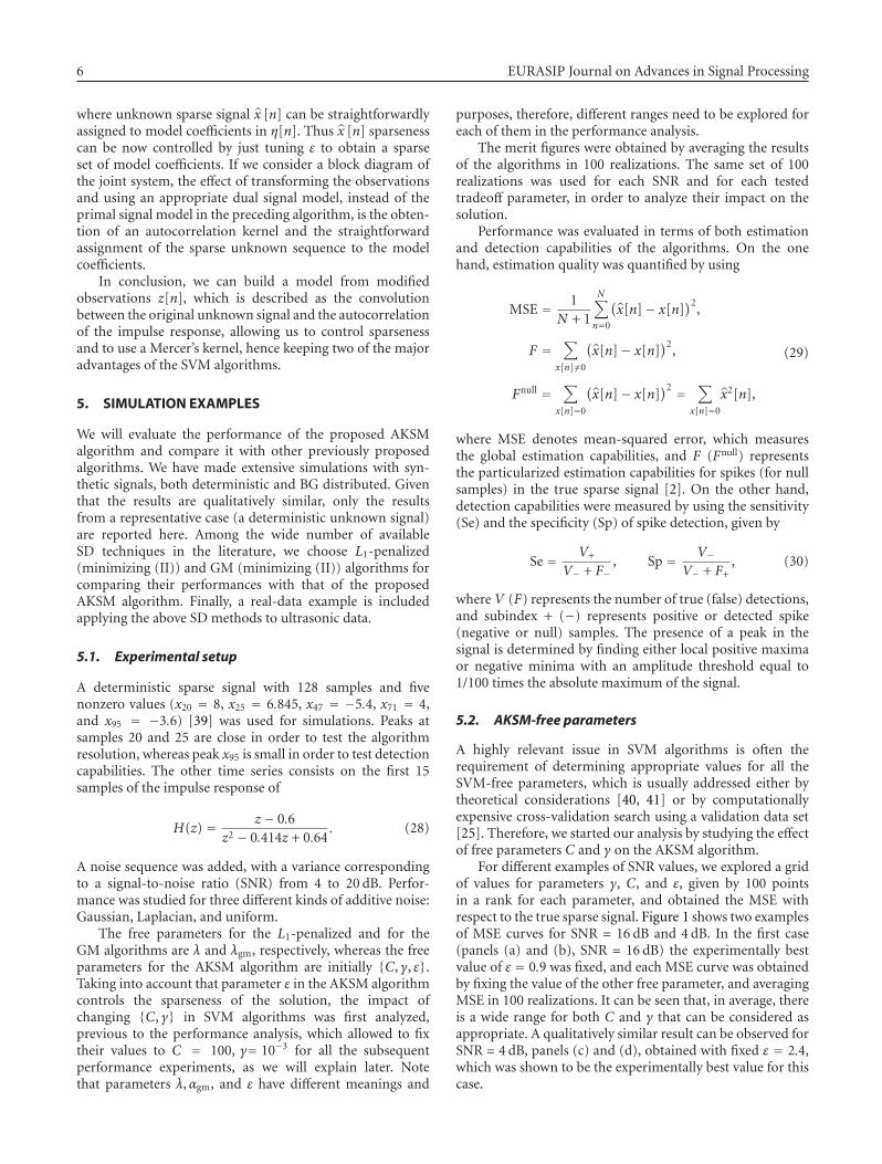
For different examples of SNR values, we explored a gridof values for parameters γ, C, and ε, given by 100 pointsin a rank for each parameter, and obtained the MSE withrespect to the true sparse signal. Figure 1 shows two examplesof MSE curves for SNR = 16 dB and 4 dB. In the first case(panels (a) and (b), SNR = 16 dB) the experimentally bestvalue of ε = 0.9 was fixed, and each MSE curve was obtainedby fixing the value of the other free parameter, and averagingMSE in 100 realizations. It can be seen that, in average, thereis a wide range for both C and γ that can be considered asappropriate. A qualitatively similar result can be observed forSNR = 4 dB, panels (c) and (d), obtained with fixed ε = 2.4,which was shown to be the experimentally best value for thiscase.

Jose Luis Rojo-Alvarez et al. 7

0

0.2

0.4

0.6

0.8

1

1.2

1.4

MSE

10−6 10−5 10−4 10−3 10−2 10−1 100 101 102 103

γ

(a)

0

0.2

0.4

0.6

0.8

1

1.2

1.4

MSE

10−3 10−2 10−1 100 101 102 103

C

(b)

0

0.2

0.4

0.6

0.8

1

1.2

1.4

MSE

10−6 10−4 10−2 100 102

γ

(c)

0

0.2

0.4

0.6

0.8

1

1.2

1.4

MSE

10−3 10−2 10−1 100 101 102 103

C

(d)

Figure 1: MSE of the AKSM algorithm as a function of free parameters γ and C in the ε-Huber cost function, with SNR = 16 dB (a,b) andSNR = 4 dB (c,d).

Therefore, aiming not to give SVM more informationthan to the other methods by means of its larger number offree parameters, C= 102 and γ= 10−3 were fixed for all thesimulations of the performance analysis.

5.3. Estimation performance

Figure 2 (panels (a), (b), and (c)) presents the MSE results forall the SD algorithms with different SNR, as a function of thefree parameter of the algorithm, that is, λ for L1-penalized,αgm for GM, and ε for AKSM. It can be seen that theoptimum value for the free parameter depends of SNR in allcases. The L1-penalized and the AKSM algorithms show lowperformance with extremely low (λ, ε → 0) and high (λ, ε >3) values of the free parameter, the optimum value being atsome intermediate point. Lower values of the free parameteryielded less-sparse solutions for all algorithms. Higher valuesof the free parameter in L1-penalized and AKSM lead toa constant value solution, clearly reached in L1-penalizedalgorithm, called the zero solution [2], which correspondsto a null-estimated sparse signal, and hence a value of MSEproportional to the norm of the true sparse signal. The GM

Table 1: Averaged MSE ± its standard deviation (×102) foroptimally chosen free parameters for each SD algorithm (best inboldface, second in italic).

Method 4 dB 10 dB 16 dB 20 dB

L1-pen. 23.9±8.9∗× 6.8± 2.9∗ 1.5±0.6∗× 0.6±0.3∗

GM 117.2± 197.6∗ 5.2±6.5 3.3± 2.0∗ 1.5± 0.3∗

AKSM 12.2± 4.5 3.2± 1.3 0.7± 0.2 0.3± 0.1∗

Denotes p < .01 for AKSM versus GM and for AKSM versus L1 compar-isons.×Denotes p < .01 for GM versus L1 comparison.

algorithm showed a stabilization for high values of the freeparameter. The qualitatively different behavior of the GMalgorithm for high values of αgm is due to the fact that, inmost cases, there was at least one detected peak. Hence thezero solution was not reached on average with this algorithm.

Mean and standard deviation of the MSE for eachalgorithm are summarized in Table 1, showing that thehighest global estimation capabilities are always reachedby the AKSM, followed by the L1-penalized and the GMprocedures. A Wilcoxon-paired test was made to check for

8 EURASIP Journal on Advances in Signal Processing

L1

0

0.5

1

1.5

2

2.5

MSE

0 0.5 1 1.5 2 2.5 3 3.5 4

λ

(a)

GM

0

1

2

3

4

5

6

MSE

0 1 2 3 4 5 6 7 8

αgm

(b)

AKSM

0

0.5

1

1.5

2

2.5

MSE

0 1 2 3 4 5 6 7 8

ε

(c)

L1 (4 dB)

0

0.02

0.04

0.06

0.08

0.1

0.12

0.14

Fan

dF

nu

ll

0 0.5 1 1.5 2 2.5 3 3.5 4

λ

(d)

GM (4 dB)

0.02

0.04

0.060.08

0.1

0.12

0.14

0.16

0.18

0.2

Fan

dF

nu

ll

0 1 2 3 4 5 6 7 8

αgm

(e)

AKSM (4 dB)

0

0.02

0.04

0.06

0.08

0.1

0.12

0.14

Fan

dF

nu

ll

0 1 2 3 4 5 6 7 8

ε

(f)

L1 (4 dB)

00.1

0.20.30.40.50.60.70.80.9

1

Sean

dSp

0 1 2 3 4 5 6

λ

(g)

GM (4 dB)

00.1

0.20.30.40.50.60.70.80.9

1

Sean

dSp

0 1 2 3 4 5 6 7 8

αgm

(h)

AKSM (4 dB)

00.1

0.20.30.40.50.60.70.80.9

1Se

and

Sp

0 1 2 3 4 5 6 7 8

ε

(i)

Figure 2: Performance analysis for the L1-penalized algorithm (left), the GM algorithm (middle), and the AKSM algorithm (right). (a,b,c)estimation performance: averaged MSE for SNR = 4, 8, 12, and 20 dB (solid, dashed, dotted, and dash-dotted, resp.). (d,e,f) estimationperformance: averaged F (solid) and Fnull (dashed) with SNR = 4 dB. (g,h,i) detection performance: averaged Se (solid) and Sp (dashed) forSNR = 4 dB.

statistical significance in the observed differences (∗ denotesp < .01 for AKSM versus GM and for AKSM versusL1 comparisons, × denotes p < .01 for GM versus L1comparison).

In Figure 2 (panels (d), (e), and (f)), averaged F and Fnull

are depicted separately for each algorithm, for SNR = 4 dB. Ingeneral, it can be observed that the higher the free parameter,the higher F and the lower Fnull. Also saturation effects arepresent in GM for Fnull. The cross-point between both curvesrepresents a good indicator of the tradeoff between bothmerit figures, and it appears for values of the free parameter

close to the optimum in the MSE sense (i.e., for globalestimation) in all the algorithms, independently of the SNR.This suggests that the global estimation performance was notbiased towards neither of the two kinds of samples (nonnulland null) in the sparse signal.

5.4. Detection performance

Figure 2 (panels (g), (h), and (i)) shows the detectioncapabilities in terms of Se and Sp for all the algorithms.As expected, Sp (Se) increases (decreases) with the free

Jose Luis Rojo-Alvarez et al. 9

−4

−2

0

2

4

6

8

20 40 60 80 100 120

(a)

−4

−2

0

2

4

6

8

20 40 60 80 100 120

(b)

−4

−2

0

2

4

6

8

20 40 60 80 100 120

(c)

Figure 3: An example of SD results versus data with SNR = 4 dB for: (a) the L1-penalized algorithm; (b) the GM algorithm; (c) the AKSMalgorithm.

Table 2: Averaged MSE ± its standard deviation (×102) for each SD algorithm (best in bold, second in italic) under Laplacian and uniformadditive noises.

Laplacian noise Uniform noise

Method 4 dB 10 dB 16 dB 20 dB 4 dB 10 dB 16 dB 20 dB

L1-pen. 18.3 ± 8.8∗ 4.6 ± 2.6∗ 1.2 ± 0.7∗× 0.5 ± 0.3∗ 3.7 ± 1.4∗× 1.0 ± 0.4∗× 0.2 ± 0.1∗ 1.0 ± 0.03∗

GM 94.1± 108.3∗ 8.8± 13.1 3.1± 2.4∗ 2.7± 1.4∗ 12.5± 5.1 3.4± 1.2∗ 2.7± 0.5∗ 2.6± 0.3∗

AKSM 13.0± 5.6 3.6± 1.6 0.9± 0.5 0.3± 0.2 1.6± 0.6 0.4± 0.2 0.1± 0.04 0.04± 0.01

parameter, and again, the cross-point between both curvesrepresents a good working point for applications where bothdetection rates are similarly relevant. From this point of view,the detection performance of the algorithms is qualitativelysimilar to their estimation performance, that is, the highestfor AKSM (close to 100% for Se and Sp simultaneously),and for the L1-penalized and the GM methods. The value ofthe free parameter for optimal detection was again close, butnot identical, to the value of the free parameter for optimalestimation in all the algorithms.

Records of estimated signals show a high variability, butin Figure 3, we present some representative results of thosecorresponding to previously presented performance figures.Optimum values of the free parameters in this example wereused. It can be observed that L1-penalized deconvolutiondetects almost all the peaks, but it produces a number oflow amplitude spurious peaks. In the example, the GMprocedure reaches a high estimation performance and a lownumber (yet high amplitude) of spurious peaks, as well asa misdetection of a large peak. Finally, the main drawbackthat could be observed for AKSM is the systematic error inthe peak amplitude detection, due to a collateral effect ofinsensitivity caused by using ε /= 0 for yielding sparsenesson the ε-Huber cost function, but total detection was oftenattained with almost no spurious detection.

With respect to sparseness of the tested algorithms, itcan be analyzed from the merit figures for estimation andfor detection. The values of Fnull can be seen as an averagedmeasurement of sparseness of each SD method, takinginto account that similarly high values of this parametercan be given either by a large number of spurious peakswith low amplitude or by a lower number of spuriouspeaks with high amplitude. Note that, in any case, the

AKSM algorithm reaches much better values, specially whencompared to GM. Similar conclusions with respect tosparseness were obtained from the sensitivity and specificityresults.

5.5. Robustness with respect to non-Gaussian noise

Table 2 shows the estimation performance of the comparedalgorithms for Laplacian and uniform noise sources addedto the deterministic signal instead of a Gaussian noise.Optimal-free parameters were previously estimated for allthe algorithms. Again, Wilcoxon-paired test was used (∗denotes p < .01 for AKSM versus GM and for AKSMversus L1 comparisons, × denotes p < .01 for GM versusL1 comparison). In general, estimation capabilities of eachalgorithm are similar for Gaussian and Laplacian noises, anddramatically higher for uniform noise. The L1-penalized andthe AKSM algorithms still exhibits good performance in thepresence of non-Gaussian noise, whereas the GM algorithmshows slightly poorer performance, specially for low SNR.It can be seen that in the presence of both Laplacian anduniform noise, MSE is lower for ASKM in all cases.

5.6. An application example with real data

We analyze a B-scan given by an ultrasonic transducerarray from a layered composite material. An A-scan is theultrasound echo signal received by a single element in thetransducer array, and the set of A-scans obtained by eachof the elements of the array is known as B-scan. Henceeach A-scan is a time-varying signal, whereas B-scan is aspatiotemporal representation of the ultrasound. Scan dataare available at http://www.signal.uu.se/Toolbox/DT/ and

10 EURASIP Journal on Advances in Signal Processing

AKSM

L1

GM

100 200 300

100 200 300

100 200 300

AKSM

L1

GM

100 200 300

100 200 300

100 200 300

0

0.2

0.4

0

0.2

0.4

0

0.2

0.4

−0.5

0

0.5

−0.5

0

0.5

−0.5

0

0.5

(a)

B-scan

0.5

0

−0.5

−1

100200

300Time

50

100

150

Space

1

0.5

0

100200

300Time

50

100

150

Space

L1

AKSM

1

0.5

0

100200

300Time

50

100

150

Space

1

0.5

0

100200

300Time

50

100

150

Space

GM

(b)

Figure 4: Real data application: deconvolution of the impulse response of a ultrasound transducer in the analysis of a layered compositematerial. (a) Example of deconvolution of a single A-scan line with each algorithm: left, sparse estimated signal; right, estimated A-line. (b)Deconvolution of the B-scan data.

Jose Luis Rojo-Alvarez et al. 11

details on this application can be found elsewhere [42].Figure 4(a) shows a signal example (A-scan) of the sparsesignal estimated by each of the tested methods, using asimpulse response a prototype obtained from the B-scan ina single line where clearly only one reflection was present.The same panel also shows the reconstructed observed signal.Noise level in the data was relatively low, and free parametersof each algorithm were adjusted accordingly to the resultsobtained with the synthetic signal example (for this purpose,a normalization of the B-scan is previously made). It can beseen a behavior qualitatively similar to the previously seenfor each algorithm, that is, the L1 algorithm yields a good-quality solution with a noticeably number of spurious peaks,the AKSM algorithm yields a good-quality solution with lessspurious peaks, and the GM algorithm fails at detecting thelow amplitude peaks that are clearly present in this A-scansignal. Figure 4(b) shows the reconstruction of the completeB-scan data, with similar behavior for all the A-scan lines.

6. CONCLUSIONS

A fully practical algorithm for SD using SVM principles,which we call the AKSM algorithm, has been introducedand evaluated. It works with the convolution of the observedsequence with the time-reversed impulse response, this waycreating an implicit autocorrelation kernel problem. Theuse of an ε-Huber cost function in the proposed algorithmprovides a high degree of robustness against the presenceof non-Gaussian additive noises. The solution is sparse asa consequence of the support vector formulation, and theimplicit regularization of all SVM algorithms helps us toobtain interesting results. These advantages can be observedin illustrative simulation setups, which serves to comparethe new algorithm performance with those of two well-known procedures, the L1-penalized and the GM modeldeconvolution algorithms. The proposed algorithm presentsan advantage in terms of both estimation and detectioncapabilities in most the situations, and there is no difficultyin finding appropriate values for its hyperparameters.

Further effort will be devoted to expand the SVM princi-ples presented here to obtain improved algorithms in otherrelevant signal and image-processing problems, speciallythose useful for spectral analysis and image denoizing anddeblurring.

APPENDICES

A. PSM DUAL PROBLEM

Instead of making the full derivation of the PSM algorithmin (15), a fast method can be used from the linear signal-processing framework in [28]. In brief, be {y[n]} a discretetime series, observations with noise, and be {zp[n], p =0, . . . ,N} a vector basis of the reconstruction signal space.Then the general linear model can be expressed as

y[n] =N∑

p=0

wpzp[n] + e[n]. (A.1)

The linear framework for SVM linear signal models requiresto determine, at the begining, the transversal vector of thesignal space basis, given by vs = [z0[s], z1[s], . . . , zN [s]]T ;then, to obtain the elements of the SV algorithm isstraightforward. In our case, we can see from (1) that thesignal space is generated by the time-shifted versions of theimpulse response, that is, zp[n] = h[n − p], and then, thepth coefficient vector of the linear model is just the pthsample of the unknown sparse signal, that is, wp = x[p].Therefore, the transversal vector is just vs = [h[s],h[s −1],h[s − 2], . . . ,h[s − N]]T , so that the dot product matrixis given by R(i, l) = vTi , vl =

∑Pk=0h[i − k]h[l − k] for

this problem statement, and the unknown signal is given by(16).

Then the dual problem consists on maximizing

−12

(

α−α∗)T(R + γI)(

α−α∗) +(

α−α∗)Ty − ε1T(

α+α∗)

(A.2)

constrained to 0 ≤ α(∗) ≤ C, where 1 denotes an all onescolumn vector, I denotes the identity matrix, α[n], α[n]∗

are the Lagrange multipliers associated to the positive andnegative parts of residuals e[n] as usual in SVM, α(∗) =[α(∗)

0 , . . . ,α(∗)N ]T , and y = [y[0], . . . , y[N]]T . This is a

quadratic programming (QP) problem, from which solution(16) is obtained.

B. AKSM DUAL PROBLEM

As usual in SVM regression algorithms, the optimizationof (23) leads to a dual problem to be optimized, whichyields model coefficients η[n] from Lagrange multipliersα[n], α[n]∗, that are associated to residuals e[n]. In this case,the elements of the Gram matrix of the problem are found tobe

T(i, l) = φ(i)Tφ(l) = K(i, l) = Rh[i− l], (B.1)

and accordingly, the dual problem can be easily shown toconsist on the maximization of

−12

(

α− α∗)T

(T + γI)(

α− α∗)

+(

α− α∗)T

z− ε1T(

α + α∗)

(B.2)

subject to 0 ≤ α(∗) ≤ C, which is formally identical to the QPproblem in (A.2). A detailed derivation of the dual problemcan be seen in [31] for the signal-processing application ofdiscrete time series interpolation.

ACKNOWLEDGMENT

This work has been partly supported by research projectsS-0505/TIC/0223 (Madrid Government), TEC2007-68096-C02/TCM, and TEC2005-00992, ESP2005-07724-C05-03,TEC2006-13845/TCM, and CONSOLIDER/CSD2007-00018(Spanish MEC).

12 EURASIP Journal on Advances in Signal Processing

REFERENCES

[1] J. Mendel and C. S. Burrus, Maximum-Likelihood Deconvolu-tion: A Journey into Model-Based Signal Processing, Springer,New York, NY, USA, 1990.

[2] M. S. O’Brien, A. N. Sinclair, and S. M. Kramer, “Recovery ofa sparse spike time series by L1 norm deconvolution,” IEEETransactions on Signal Processing, vol. 42, no. 12, pp. 3353–3365, 1994.

[3] N. P. Galatsanos, A. K. Katsaggelos, R. T. Chin, and A. D.Hillery, “Least squares restoration of multichannel images,”IEEE Transactions on Signal Processing, vol. 39, no. 10, pp.2222–2236, 1991.

[4] W. S. Ellis, S. J. Eisenberg, D. M. Auslander, M. W. Dae,A. Zakhor, and M. D. Lesh, “Deconvolution: a novel signalprocessing approach for determining activation time fromfractionated electrograms and detecting infarcted tissue,”Circulation, vol. 94, no. 10, pp. 2633–2640, 1996.

[5] S. M. Kay, Fundamentals of Statistical Signal Processing:Estimation Theory, Prentice Hall, Englewood Cliffs, NJ, USA,1993.

[6] B. Rice, “Inverse convolution filters,” Geophysics, vol. 27, no. 1,pp. 4–18, 1962.

[7] J. Claerbout and E. A. Robinson, “The error in least-squaresinverse filtering,” Geophysics, vol. 29, no. 1, pp. 118–120, 1964.

[8] W. T. Ford and J. H. Hearne, “Least-squares inverse filtering,”Geophysics, vol. 31, no. 5, pp. 917–926, 1966.

[9] A. J. Berkhout, “Least-squares inverse filtering and waveletdeconvolution,” Geophysics, vol. 42, no. 7, pp. 1369–1383,1977.

[10] A. Tikhonov and V. Y. Arsenin, Solutions to Ill-Posed Problems,Winston & Sons, Washington, DC, USA, 1977.

[11] A. E. Hoerl and R. W. Kennard, “Ridge regression: biasedestimation for nonorthogonal problems,” Technometrics, vol.12, no. 1, pp. 55–67, 1970.

[12] S. Huffel and J. Vanderwalle, The Total Least Squares Problem:Computational Aspects and Analysis, SIAM, Philadelphia, Pa,USA, 1991.

[13] Y. C. Eldar and A. V. Oppenheim, “Covariance shaping least-squares estimation,” IEEE Transactions on Signal Processing,vol. 51, no. 3, pp. 686–697, 2003.

[14] C. Narduzzi, “Inverse filtering with signal-adaptive con-straints,” IEEE Transactions on Instrumentation and Measure-ment, vol. 54, no. 4, pp. 1553–1559, 2005.

[15] H. Taylor, S. Banks, and J. F. McCoy, “Deconvolution with theL1 norm,” Geophysics, vol. 44, no. 1, pp. 39–52, 1979.

[16] S. S. Chen, D. L. Donoho, and M. A. Saunders, “Atomicdecomposition by basis pursuit,” SIAM Review, vol. 43, no. 1,pp. 129–159, 2001.

[17] J. Kormylo and J. Mendel, “Maximum likelihood detectionand estimation of Bernoulli-Gaussian processes,” IEEE Trans-actions on Information Theory, vol. 28, no. 3, pp. 482–488,1982.

[18] I. Santamarıa-Caballero, C. J. Pantaleon-Prieto, and A. Artes-Rodrıguez, “Sparse deconvolution using adaptive mixed-Gaussian models,” Signal Processing, vol. 54, no. 2, pp. 161–172, 1996.

[19] Y. C. Eldar and N. Merhav, “A competitive minimax approachto robust estimation of random parameters,” IEEE Transac-tions on Signal Processing, vol. 52, no. 7, pp. 1931–1946, 2004.

[20] Y. C. Eldar, A. Ben-Tal, and A. Nemirovski, “Linear minimaxregret estimation of deterministic parameters with boundeddata uncertainties,” IEEE Transactions on Signal Processing, vol.52, no. 8, pp. 2177–2188, 2004.

[21] Y. C. Eldar, A. Ben-Tal, and A. Nemirovski, “Robust mean-squared error estimation in the presence of model uncertain-ties,” IEEE Transactions on Signal Processing, vol. 53, no. 1, pp.168–181, 2005.

[22] Y. C. Eldar, “Robust deconvolution of deterministic andrandom signals,” IEEE Transactions on Information Theory,vol. 51, no. 8, pp. 2921–2929, 2005.

[23] R. Neelamani, H. Choi, and R. Baraniuk, “ForWaRD: fourier-wavelet regularized deconvolution for ill-conditioned sys-tems,” IEEE Transactions on Signal Processing, vol. 52, no. 2,pp. 418–433, 2004.

[24] S. A. Kassam and H. V. Poor, “Robust techniques for signalprocessing: a survey,” Proceedings of the IEEE, vol. 73, no. 3,pp. 433–481, 1985.

[25] V. Vapnik, Statistical Learning Theory, John Wiley & Sons, NewYork, NY, USA, 1998.

[26] G. Camps-Valls, J. L. Rojo-Alvarez, and M. Martınez-Ramon,Eds., Kernel Methods in Bioengineering, Signal, and ImageProcessing, Idea Group, Hershey, Pa, USA, 2007.

[27] J. Mercer, “Functions of negative and positive type andtheir connection with the theory of integral equations,”Philosophical Transactions of the Royal Society of London A, vol.209, pp. 415–446, 1909.

[28] J. L. Rojo-Alvarez, G. Camps-Valls, M. Martınez-Ramon,E. Soria-Olivas, A. Navia-Vazquez, and A. R. Figueiras-Vidal, “Support vector machines framework for linear signalprocessing,” Signal Processing, vol. 85, no. 12, pp. 2316–2326,2005.

[29] J. L. Rojo-Alvarez, M. Martınez-Ramon, M. de Prado-Cumplido, A. Artes-Rodrıguez, and A. R. Figueiras-Vidal,“Support vector method for robust ARMA system identifica-tion,” IEEE Transactions on Signal Processing, vol. 52, no. 1, pp.155–164, 2004.

[30] G. Camps-Valls, L. Bruzzone, J. L. Rojo-Alvarez, and F.Melgani, “Robust support vector regression for biophysicalvariable estimation from remotely sensed images,” IEEEGeoscience and Remote Sensing Letters, vol. 3, no. 3, pp. 339–343, 2006.

[31] J. L. Rojo-Alvarez, C. Figuera-Pozuelo, C. E. Martınez-Cruz,G. Camps-Valls, F. Alonso-Atienza, and M. Martınez-Ramon,“Nonuniform interpolation of noisy signals using supportvector machines,” IEEE Transactions on Signal Processing, vol.55, no. 8, pp. 4116–4126, 2007.

[32] F. Girosi, M. Jones, and T. Poggio, “Regularization theory andneural networks architectures,” Neural Computation, vol. 7,no. 2, pp. 291–269, 1995.

[33] T. Poggio and S. Smale, “The mathematics of learning: dealingwith data,” Notices of the American Mathematical Society, vol.50, no. 5, pp. 537–544, 2003.

[34] M. A. Aizerman, E. M. Braverman, and L. Rozoner, “Theoret-ical foundations of the potential function method in patternrecognition learning,” Automation and Remote Control, vol. 25,pp. 821–837, 1964.

[35] J. Shawe-Taylor and N. Cristianini, Kernel Methods for PatternAnalysis, Cambridge University Press, Cambridge, UK, 2004.

[36] L. Zhang, W. Zhou, and L. Jiao, “Wavelet support vectormachine,” IEEE Transactions on Systems, Man, and CyberneticsB, vol. 34, no. 1, pp. 34–39, 2004.

[37] J. Suykens, “Support vector machines: a nonlinear modellingand control perspective,” European Journal of Control, vol. 7,no. 2-3, pp. 311–327, 2001.

Jose Luis Rojo-Alvarez et al. 13

[38] D. Mattera and S. Haykin, “Support vector machines fordynamic recostruction of chaotic systems,” in Advances inKernel Methods, pp. 211–242, MIT Press, Cambridge, Mass,USA, 1999.

[39] A. R. Figueiras-Vidal, D. Docampo-Amoedo, J. R. Casar-Corredera, and A. Artes-Rodrıguez, “Adaptive iterative algo-rithms for spiky deconvolution,” IEEE Transactions on Acous-tics, Speech, and Signal Processing, vol. 38, no. 8, pp. 1462–1466, 1990.

[40] J. T. Kwok and I. W. Tsang, “Linear dependency betweenε and the input noise in ε-support vector regression,” IEEETransactions on Neural Networks, vol. 14, no. 3, pp. 544–553,2003.

[41] V. Cherkassky and Y. Ma, “Practical selection of SVMparameters and noise estimation for SVM regression,” NeuralNetworks, vol. 17, no. 1, pp. 113–126, 2004.

[42] T. Olofsson, “Semi-sparse deconvolution robust to uncertain-ties in the impulse responses,” Ultrasonics, vol. 42, no. 1–9, pp.969–975, 2004.

Photograph © Turisme de Barcelona / J. Trullàs

Preliminary call for papers

The 2011 European Signal Processing Conference (EUSIPCO 2011) is thenineteenth in a series of conferences promoted by the European Association forSignal Processing (EURASIP, www.eurasip.org). This year edition will take placein Barcelona, capital city of Catalonia (Spain), and will be jointly organized by theCentre Tecnològic de Telecomunicacions de Catalunya (CTTC) and theUniversitat Politècnica de Catalunya (UPC).EUSIPCO 2011 will focus on key aspects of signal processing theory and

li ti li t d b l A t f b i i ill b b d lit

Organizing Committee

Honorary ChairMiguel A. Lagunas (CTTC)

General ChairAna I. Pérez Neira (UPC)

General Vice ChairCarles Antón Haro (CTTC)

Technical Program ChairXavier Mestre (CTTC)

Technical Program Co Chairsapplications as listed below. Acceptance of submissions will be based on quality,relevance and originality. Accepted papers will be published in the EUSIPCOproceedings and presented during the conference. Paper submissions, proposalsfor tutorials and proposals for special sessions are invited in, but not limited to,the following areas of interest.

Areas of Interest

• Audio and electro acoustics.• Design, implementation, and applications of signal processing systems.

l d l d d

Technical Program Co ChairsJavier Hernando (UPC)Montserrat Pardàs (UPC)

Plenary TalksFerran Marqués (UPC)Yonina Eldar (Technion)

Special SessionsIgnacio Santamaría (Unversidadde Cantabria)Mats Bengtsson (KTH)

FinancesMontserrat Nájar (UPC)• Multimedia signal processing and coding.

• Image and multidimensional signal processing.• Signal detection and estimation.• Sensor array and multi channel signal processing.• Sensor fusion in networked systems.• Signal processing for communications.• Medical imaging and image analysis.• Non stationary, non linear and non Gaussian signal processing.

Submissions

Montserrat Nájar (UPC)

TutorialsDaniel P. Palomar(Hong Kong UST)Beatrice Pesquet Popescu (ENST)

PublicityStephan Pfletschinger (CTTC)Mònica Navarro (CTTC)

PublicationsAntonio Pascual (UPC)Carles Fernández (CTTC)

I d i l Li i & E hibiSubmissions

Procedures to submit a paper and proposals for special sessions and tutorials willbe detailed at www.eusipco2011.org. Submitted papers must be camera ready, nomore than 5 pages long, and conforming to the standard specified on theEUSIPCO 2011 web site. First authors who are registered students can participatein the best student paper competition.

Important Deadlines:

P l f i l i 15 D 2010

Industrial Liaison & ExhibitsAngeliki Alexiou(University of Piraeus)Albert Sitjà (CTTC)

International LiaisonJu Liu (Shandong University China)Jinhong Yuan (UNSW Australia)Tamas Sziranyi (SZTAKI Hungary)Rich Stern (CMU USA)Ricardo L. de Queiroz (UNB Brazil)

Webpage: www.eusipco2011.org

Proposals for special sessions 15 Dec 2010Proposals for tutorials 18 Feb 2011Electronic submission of full papers 21 Feb 2011Notification of acceptance 23 May 2011Submission of camera ready papers 6 Jun 2011