SPARSE PARAMETRIZATION OF PLANE CURVES
20
Johann Radon Institute for Computational and Applied Mathematics Austrian Academy of Sciences (ÖAW) RICAM-Report No. 2005-08 T. Beck, J. Schicho Sparse Parametrization of Plane Curves Powered by TCPDF (www.tcpdf.org)
-
Upload
independent -
Category
Documents
-
view
2 -
download
0
Transcript of SPARSE PARAMETRIZATION OF PLANE CURVES
Johann Radon Institutefor Computational and Applied MathematicsAustrian Academy of Sciences (ÖAW)
RICAM-Report No. 2005-08
T. Beck, J. Schicho
Sparse Parametrization of Plane Curves
Powered by TCPDF (www.tcpdf.org)
SPARSE PARAMETRIZATION OF PLANE CURVES
TOBIAS BECK AND JOSEF SCHICHO
Abstract. We present a new method for the rational parametrization of planealgebraic curves. The algorithm exploits the shape of the Newton polygon ofthe defining implicit equation and is based on methods of toric geometry.
Contents
1. Introduction 22. Preliminaries on Toric Varieties 22.1. Embedding the curve into a complete toric surface 22.2. Toric invariant divisors 52.3. Linear systems of toric invariant divisors 53. Sparse Parametrization 63.1. The genus 63.2. The parametrizing linear system 63.3. The algorithm 93.4. An example 104. Another Proof of Correctness 144.1. Some exact sequences 144.2. The sheaf on the normalized curve 154.3. Reduction of the parametrization problem to rational normal curves 154.4. Vanishing of the first cohomology 165. Conclusion 18References 18
Date: June 6, 2005.The authors were supported by the FWF (Austrian Science Fund) in the frame of the research
projects SFB 1303 and P15551.
1
2 TOBIAS BECK AND JOSEF SCHICHO
1. Introduction
Given a bivariate polynomial f ∈ K[x, y] over some field K we will describe amethod to find a proper parametrization of the curve defined implicitly by f . Thatis we will find (X(t), Y (t)) ∈ K(t) s.t. f(X(t), Y (t)) = 0 and (X(t), Y (t)) inducesa birational morphism from the curve to the affine line. This is the problem offinding a rational parametrization, a well-studied subject in algebraic geometry.There are already several algorithms, e.g. [10] and [14]. But up to now thesemethods do not take into account whether the defining equation is sparse or not.We will present an algorithm which exploits the shape of the Newton polygon ofthe defining polynomial by embedding the curve in a well-chosen complete surface.In this article we do not care for the involved extensions of the coefficient field andtherefore assume that K is algebraically closed.
This article is organized as follows. In section 2 we recall some basic constructionsof toric geometry. In particular we show how to embed a curve into a suitablecomplete toric surface. In section 3 we show how to compute the genus of the curvein this setting and how to find a linear system of rational functions on the curvethat allows to find a parametrization. We state the main theorem which provesthe algorithm to be correct. Finally we give a coarse description of the algorithmin pseudo-code and an example. The last section is devoted to a different proof ofcorrectness using sheaf theoretical and cohomological arguments.
The reason for giving two different proofs is a historical one. When constructingthe algorithm, we were looking for a suitable vector space of rational functionsfor the parametrization map. We found it by computing the first cohomology ofcertain sheaves of rational functions. Afterwards it turned out that more elementaryarguments (using only the notion of divisors) can also be used to prove correctnessof the algorithm. So in one sense the second proof is redundant. We decided to keepit nevertheless in the hope that it provides additional insight. When not seen inanother context, the fact that a certain vector space has exactly the right dimensionlooks like a nice coincidence.
2. Preliminaries on Toric Varieties
Let K be an algebraically closed field. We are going to parametrize (if possible) aplane curve F ′ that is given by an absolutely irreducible polynomial f ∈ K[x, y] onthe torus T := (K∗)2. Actually we will study a curve F which is the Zariski closureof F ′ in a complete surface containing the torus, i.e. F ∩T = F ′. We will first showhow to realize this surface and then recall some basic definitions and propositions.A good introduction to toric varieties can be found in [2].
2.1. Embedding the curve into a complete toric surface. Parametrization byrational functions is a “global problem”. In order to apply some theorems of globalcontent we have to embed T in a complete surface. One possible complete surface,which is often used in this context, is the projective plane P2
K. We will choose acomplete toric surface instead, whose construction is guided by the shape of theNewton polygon of f . In fact also P2
K is a complete toric surface and correspondsto the Newton polygon of a dense polynomial f .
The Newton polygon Π(f) ⊂ R2 is defined as the convex hull of all lattice points(r, s) ∈ Supp(f) (i.e. all (r, s) ∈ Z2 s.t. xrys appears with a non-zero coefficient inf). For instance, if f is dense of total degree d then the Newton polygon is equal

SPARSE PARAMETRIZATION OF PLANE CURVES 3
s
r
v5 = v6
v4
v3
v1 v2
v7 = v0
h2
Π(f)
(a2, b2)e2
Figure 1. Newton polygonNewton polygon Π(f) with n = 7 vertices vi. We emphasize edge e2 and show its normal vector(a2, b2) = (−1, 1) and the support half plane h2. Here we would get c2 = −3. The procedure oflemma 1 inserts an extra normal vector and thus we have the “double” vertex v5 = v6.
to the triangle with vertices (0, 0), (d, 0) and (0, d). A sample Newton polygonis illustrated in figure 1. Throughout this article we will always implicitly assumethat Π(f) is non-degenerate; if f is irreducible and Π(f) is a line segment or a pointthen the support of f has cardinality at most 2 and the parametrization problemis trivial.
For any pair of relatively prime a, b ∈ Z, let c(a, b) ∈ Z be the minimum valueof ar + bs, where (r, s) ∈ Π(f). Then Π(f) is a finite intersection of say n supporthalf planes
hi := {(r, s) ∈ R2 | air + bis ≥ ci} where ci := c(ai, bi).
We assume that the (ai, bi) are arranged cyclically, i.e. ai−1bi − aibi−1 > 0 (settinga0 := an and b0 := bn). We also give names to the edges and the vertices ofintersection
ei := {(r, s) ∈ R2 | air + bis = ci} and vi := ei ∩ ei−1.
Note that the set of half planes is not uniquely defined, there may be redundant halfplanes where the edge meets Π(f) in one vertex (in this case, some of the verticesvi will coincide).
Lemma 1. We can assume that ai−1bi − aibi−1 = 1 for 1 < i ≤ n.
Proof. The values ai−1bi − aibi−1 are invariant under unimodular transformations(i.e. linear transformations by an integral matrix with determinant 1). Assume thatai0−1bi0 − ai0bi0−1 > 1 for some i0. By a suitable unimodular transformation wemay assume (ai0 , bi0) = (0, 1). It follows that ai0−1 > 1.

4 TOBIAS BECK AND JOSEF SCHICHO
We insert a new index, for simplicity say i0 − 12 , set ai0− 1
2:= 1 and determine
bi0− 12
by integer division s.t. 0 ≤ ai0−1bi0− 12− bi0−1 < ai0−1. It follows
ai0− 12bi0 − ai0bi0− 1
2= 1 · 1− 0 · bi0− 1
2= 1 and
ai0−1bi0− 12− ai0− 1
2bi0−1 = ai0−1bi0− 1
2− 1 · bi0−1 < ai0−1
= ai0−1 · 1− 0 · bi0−1 = ai0−1bi0 − ai0bi0−1.
By inserting the additional support half plane with normal vector (ai0− 12, bi0− 1
2)
and support line through the vertex vi0 , we “substitute” the value ai0−1bi0−ai0bi0−1
by the smaller value ai0−1bi0− 12− ai0− 1
2bi0−1 and add ai0− 1
2bi0 − ai0bi0− 1
2= 1 to
the list. All other values stay fixed. Repeating this process the statement in theproposition can be achieved. �
Now we construct the toric surface. Let 1 ≤ i ≤ n and set Ui := A2K (again
identifying U0 and Un) with coordinates ui and vi. We denote the coordinate axes
by Li := {(ui, vi) ∈ Ui | ui = 0} and Ri := {(ui, vi) ∈ Ui | vi = 0} and define anopen embedding of the torus
φi : T → A2K : (x, y) 7→ (ui, vi) = (xbiy−ai , x−bi−1yai−1).
Its isomorphic image is Ti = Ui \ (Li ∪ Ri) and on Ti the morphism φi has theinverse
(ui, vi) 7→ (x, y) = (uai−1
i vaii , ubi−1
i vbii ).
For 1 ≤ i ≤ n we define isomorphisms
ψi−1,i : Ui−1 \Ri−1 → Ui \ Li : (ui−1, vi−1) 7→ (ui, vi) = (uai−2bi−aibi−2
i−1 vi−1, u−1i−1)
with inverses
ψi,i−1 := ψ−1i−1,i : (ui, vi) 7→ (ui−1, vi−1) = (v−1
i , uivai−2bi−aibi−2
i ).
For two non-neighboring indices i and j, we get isomorphisms ψi,j := φj ◦ φ−1i :
Ti → Tj . The ψi,j then satisfy the gluing conditions ψj,k ◦ ψi,j = ψi,k wheneverboth sides are defined. Hence they describe an abstract variety V , the toric surfacedefined by Π(f).
Via the gluing construction, each Ui corresponds to an isomorphic open subsetUi ⊂ V which together cover V . For any index i the open subset Ui−1 ∩ Ui cor-
responds to the two open subsets Ui−1 \ Ri−1 and Ui \ Li that are isomorphic by
ψi−1,i. The union of the sets corresponding to Ri−1 ⊂ Ui−1 and Li ⊂ Ui is a curvein V isomorphic to P1
K which we call edge curve and denote by Ei. The curves Ei−1
and Ei intersect transversally in a point Vi ∈ Ui, corresponding to (0, 0) ∈ Ui. Fornon-neighboring indices i and j the edge curves Ei and Ej are disjoint. The com-plement of the union of all edge curves is the torus T , which is also the intersectionof all open sets Ui.
Now the curve F given by f is defined to be the Zariski closure of F ′ in V . Wewill see its local equations in the next section. For the rest of the article we fixf and the corresponding curve F ⊂ V , i.e. in particular the data ai, bi, ci derivedfrom its Newton polygon.
Remark 2. The proof of lemma 1 corresponds to the resolution procedure for toricsurfaces. Being covered by affine planes A2
K the constructed toric surface is actuallysmooth. For the parametrization algorithm this is not strictly necessary (although
SPARSE PARAMETRIZATION OF PLANE CURVES 5
it may be useful). Also the theoretical arguments that follow do not really need asmooth surface. Everything would go through as well using affine toric charts. Weuse this construction mainly for simplifying notation.
2.2. Toric invariant divisors. Irreducible curves on V are also called prime(Weil) divisors. A general divisor D is defined to be a formal sum (i.e. a linearcombination over Z) of prime divisors. The set of divisors forms a free Abeliangroup Div(V ). The edge curves Ei of the previous section are the special “toricinvariant” prime divisors. Consequently a toric invariant divisor is a formal sumof the Ei. One associates to a rational function g ∈ K(x, y) its principal divisor(g). Roughly speaking g has poles and zeros on V along certain subvarieties ofcodimension one; then (g) is the divisor of zeros minus the divisor of poles (withmultiplicities). For a detailed introduction to divisors we refer to [12]. Two divisorsare called linearly equivalent iff they differ only by a principal divisor. The divisorclass group is defined as the group of divisors modulo this equivalence.
The coordinate ring of the torus is K[x, y, x−1, y−1] which is a unique factoriza-tion domain. Hence any divisor on the torus is a principal divisor and the classgroup is trivial. This implies that the class group of the surface V is generatedby the toric invariant divisors Ei. We will now show how to find representants interms of these divisors.
Lemma 3. Let g ∈ K[x, y, x−1, y−1]. Then g defines a curve on the torus T . LetG be its closure in the surface V . Then the divisor G is linearly equivalent to G0 =∑
1≤i≤n−ciEi where ci = min(r,s)∈Supp(g)(air+ bis), more precisely G = G0 + (g).
Proof. On the affine open subset Ui let
gi(ui, vi) := u−ci−1
i v−cii g(uai−1
i vaii , ubi−1
i vbii ).
Then gi ∈ K[ui, vi] is the local equation of G. Further gi differs from u−ci−1
i v−cii
only by the rational function g which is the same on each affine open set. Togetherwe see that G = G0 + (g). �
This result holds for any g ∈ K[x, y, x−1, y−1] and of course in particular forg = f , G = F and ci = ci from section 2.1. From the proof we get the localequations of the curve F embedded in V
fi(ui, vi) := u−ci−1
i v−cii f(uai−1
i vaii , ubi−1
i vbii )(1)
and a linearly equivalent divisor F0 :=∑
1≤i≤n−ciEi. Note that the divisor G0 inthe proposition depends only on the support of g, so we define:
Definition 4. Given a lattice polygon Π ∈ R2. We define the associated divisordiv(Π) :=
∑1≤i≤n−ciEi with ci = min(r,s)∈Π(air + bis).
With this definition of course div(Π(g)) = G0. In the sequel we will mainly dealwith toric invariant divisors.
2.3. Linear systems of toric invariant divisors. A divisor D is called effective(or greater or equal to 0) iff it is a non-negative sum of prime divisors. The linearsystem of rational functions associated to a divisor D is the vector space of rationalfunctions g ∈ K(x, y) s.t. D + (g) is effective. If D is in particular a toric invariantdivisor, then (g) must not have any poles on the torus. Thus we define:

6 TOBIAS BECK AND JOSEF SCHICHO
Definition 5. Given a toric invariant divisor D ∈ Div(V ), we define the linear
system L(D) := {g ∈ K[x, y, x−1, y−1] | (g) +D ≥ 0}.As a corollary to lemma 3 we see that if the divisor is given by a lattice polygon
this linear system is non-empty and has a simple description.
Corollary 6. Let Π ∈ R2 be a lattice polygon, let D = div(Π) =∑
1≤i≤n−ciEiand define Π :=
⋂1≤i≤n{(r, s) ∈ R2 | air + bis ≥ ci}. Then L(D) = 〈xrys〉(r,s)∈Π
as a K-vector space.
Here Π is the smallest polygon containing Π and given by an intersection oftranslates of the half planes hi.
3. Sparse Parametrization
It is well-known that a curve is parametrizable iff it has genus 0. In this sectionwe will first show how to compute the genus in our setting. Afterwards we givea linear system of rational functions that is used to find the parametrizing map.Finally we describe the algorithm and execute it on an example.
3.1. The genus. If the curve F was embedded in the projective plane P2K and had
total degree d , we would have the genus formula g(C) = (d−1)(d−2)2 −∑P∈C δP .
The number δP is a measure of singularity, which is defined as the dimension ofthe quotient of the integral closure of the local ring by the local ring at P (cf. [7,exercise IV.1.8]). For instance, if P is an ordinary singularity of multiplicity µ, i.e.
a self-intersection point where µ branches meet transversally, then δP = µ(µ−1)2 . In
particular the sum may be restricted to range over all singular points P ∈ C. IfΠ ⊂ R2 is a bounded domain we denote by #(Pi) := |Π∩Z2| the number of latticepoints in Π. We also write Π◦ for the interior of a domain. In the toric situationthe genus can be computed as follows:
Proposition 7. The genus of F is equal to the number of interior lattice points ofΠ(f) minus the sum of the δ-invariants of all points of F :
g(F ) = #(Π(f)◦)−∑
P∈FδP
(The sum actually ranges over the singular points of F only.)
Proof. Let F → F be the normalization of the curve. The genus of F can be definedas the arithmetic genus ga(F ) of its normalization. It is known that ga(F ) =ga(F )−∑P∈F δP (cf. [7, exercise IV.1.8]).
The fact that the arithmetic genus ga(F ) equals the number of interior latticepoints of Π(f) is a consequence of the adjunction formula (cf. [4, p. 91]). �3.2. The parametrizing linear system. First we define a family of special divi-sors on V .
Definition 8. Choose 1 ≤ m < n and let
c′i =
{ci if 1 ≤ i ≤ m andci + 1 else
where the ci originate from the lattice polygon Π(f). We define Dm := F0 −∑m+1≤i≤n Ei =
∑1≤i≤n−c′iEi ∈ Div(V ) and denote by di := #(ei)−1 the number
of lattice points on the edge i. Further we define the constant dm :=∑
1≤i≤m di.
SPARSE PARAMETRIZATION OF PLANE CURVES 7
From now on fix such an m. Note that we deliberately excluded m = n. Nowwe compute the intersection number F0 ·Dm, i.e. the number of intersections of F0
and Dm counting multiplicities.
Lemma 9. If dm ≥ 2 then F0 ·Dm = 2#(Π(f)◦) + dm − 2.
Proof. Let vi0 = (ri0 , si0) be the vertex of Π(f) common to the edges ei0−1 and ei0 .The intersection number is invariant w.r.t. linear equivalence of divisors. Then
F0 · Ei0 = (F0 + (xri0 ysi0 )) · Ei0=
(∑1≤i≤n−ciEi +
∑1≤i≤n(airi0 + bisi0)Ei
)· Ei0
=∑
1≤i≤n(−ci + airi0 + bisi0)Ei · Ei01)= (−ci0−1 + ai0−1ri0 + bi0−1si0)Ei0−1 · Ei0
+ (−ci0 + ai0ri0 + bi0si0)Ei0 ·Ei0+ (−ci0+1 + ai0+1ri0 + bi0+1si0)Ei0+1 · Ei0
2)= ai0+1(ri0 − ri0+1) + bi0+1(si0 − si0+1)
= 〈(ai0+1, bi0+1), (ri0 − ri0+1, si0 − si0+1)〉
where 1) holds because Ei and Ei0 are disjoint for non-neighboring indices i and i0and 2) holds because of the choice of (ri0 , si0) and Ei0 , Ei0+1 intersecting transver-sally. Finally the vector (ri0 − ri0+1, si0 − si0+1) is equal to di0(−bi0 , ai0) (be-cause gcd(ai0 , bi0) = 1). Computing the scalar product and applying the identityai0bi0+1 − bi0ai0+1 = 1 yields F · Ei0 = di0 .
Further we compute
F0 ·Dm = F0 · F0 − F0 ·∑m+1≤i≤nEi
1)= 2V ol(Γ)−∑m+1≤i≤n di2)=
(2#(Π(f)◦)− 2 +
∑1≤i≤n di
)−∑m+1≤i≤n di
= 2#(Π(f)◦) + dm − 2
where 1) follows from the self-intersection formula for toric invariant divisors and2) from Pick’s formula (cf. [4, pp. 111 and 113]). �
We can also determine the dimension of the associated linear system.
Lemma 10. We have dimK(L(Dm)) = #(Π(f)◦) + dm − 1.
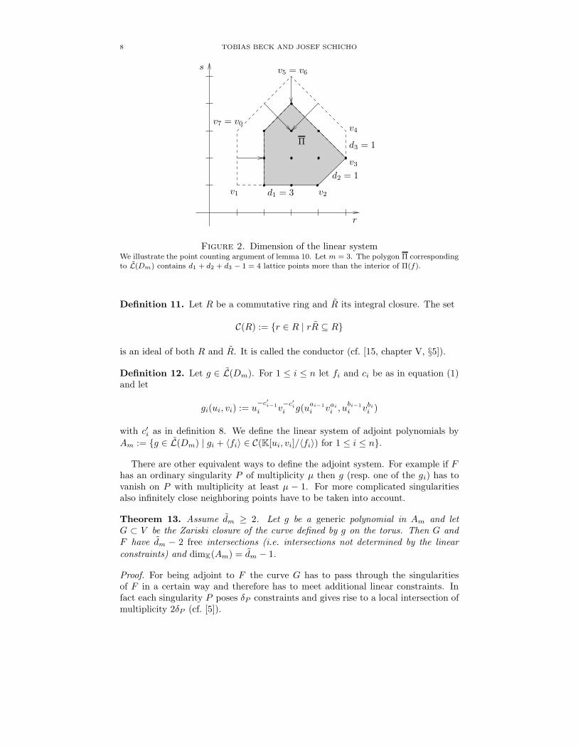
Proof. The divisor Dm is associated to a lattice polygon Π which is obtained “bysubtracting certain edges of Π(f)”, compare figure 2. For the number of latticepoints one verifies the formula
#(Π) = #(Π(f)) −(∑
m+1≤i≤n di)− 1 = #(Π(f)◦) + dm − 1.
But Π is already given by an intersection of translates of the half planes hi. Thelemma now follows from corollary 6. �
We define a subspace of the linear system L(Dm) by adding linear constraintsderived from conductor ideals. Afterwards we state and prove the main theorem.
8 TOBIAS BECK AND JOSEF SCHICHO
Π
s
r
v5 = v6
v4
v3
v1 v2
v7 = v0
d3 = 1
d1 = 3
d2 = 1
Figure 2. Dimension of the linear systemWe illustrate the point counting argument of lemma 10. Let m = 3. The polygon Π correspondingto L(Dm) contains d1 + d2 + d3 − 1 = 4 lattice points more than the interior of Π(f).
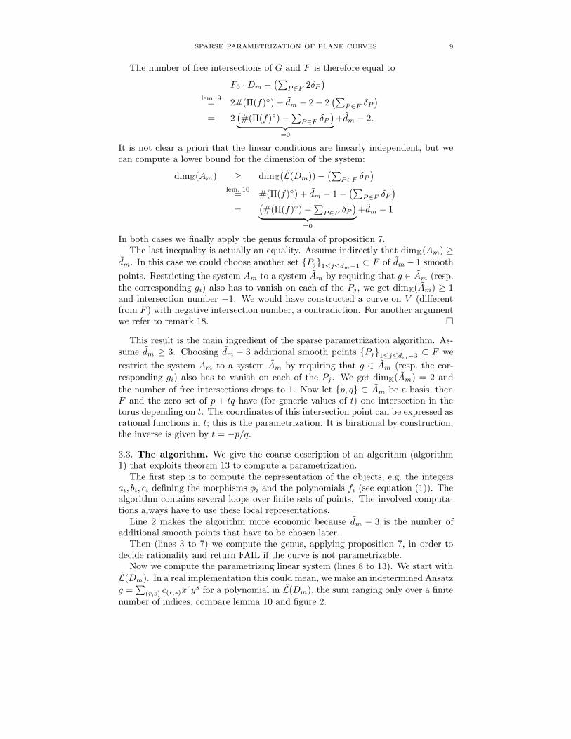
Definition 11. Let R be a commutative ring and R its integral closure. The set
C(R) := {r ∈ R | rR ⊆ R}
is an ideal of both R and R. It is called the conductor (cf. [15, chapter V, §5]).
Definition 12. Let g ∈ L(Dm). For 1 ≤ i ≤ n let fi and ci be as in equation (1)and let
gi(ui, vi) := u−c′i−1
i v−c′ii g(u
ai−1
i vaii , ubi−1
i vbii )
with c′i as in definition 8. We define the linear system of adjoint polynomials by
Am := {g ∈ L(Dm) | gi + 〈fi〉 ∈ C(K[ui, vi]/〈fi〉) for 1 ≤ i ≤ n}.
There are other equivalent ways to define the adjoint system. For example if Fhas an ordinary singularity P of multiplicity µ then g (resp. one of the gi) has tovanish on P with multiplicity at least µ − 1. For more complicated singularitiesalso infinitely close neighboring points have to be taken into account.
Theorem 13. Assume dm ≥ 2. Let g be a generic polynomial in Am and letG ⊂ V be the Zariski closure of the curve defined by g on the torus. Then G andF have dm − 2 free intersections (i.e. intersections not determined by the linear
constraints) and dimK(Am) = dm − 1.
Proof. For being adjoint to F the curve G has to pass through the singularitiesof F in a certain way and therefore has to meet additional linear constraints. Infact each singularity P poses δP constraints and gives rise to a local intersection ofmultiplicity 2δP (cf. [5]).
SPARSE PARAMETRIZATION OF PLANE CURVES 9
The number of free intersections of G and F is therefore equal to
F0 ·Dm −(∑
P∈F 2δP)
lem. 9= 2#(Π(f)◦) + dm − 2− 2
(∑P∈F δP
)
= 2(#(Π(f)◦)−∑P∈F δP
)︸ ︷︷ ︸
=0
+dm − 2.
It is not clear a priori that the linear conditions are linearly independent, but wecan compute a lower bound for the dimension of the system:
dimK(Am) ≥ dimK(L(Dm))−(∑
P∈F δP)
lem. 10= #(Π(f)◦) + dm − 1−
(∑P∈F δP
)
=(#(Π(f)◦)−∑P∈F δP
)︸ ︷︷ ︸
=0
+dm − 1
In both cases we finally apply the genus formula of proposition 7.The last inequality is actually an equality. Assume indirectly that dimK(Am) ≥
dm. In this case we could choose another set {Pj}1≤j≤dm−1 ⊂ F of dm − 1 smooth
points. Restricting the system Am to a system Am by requiring that g ∈ Am (resp.
the corresponding gi) also has to vanish on each of the Pj , we get dimK(Am) ≥ 1and intersection number −1. We would have constructed a curve on V (differentfrom F ) with negative intersection number, a contradiction. For another argumentwe refer to remark 18. �
This result is the main ingredient of the sparse parametrization algorithm. As-sume dm ≥ 3. Choosing dm − 3 additional smooth points {Pj}1≤j≤dm−3 ⊂ F we
restrict the system Am to a system Am by requiring that g ∈ Am (resp. the cor-
responding gi) also has to vanish on each of the Pj . We get dimK(Am) = 2 and
the number of free intersections drops to 1. Now let {p, q} ⊂ Am be a basis, thenF and the zero set of p + tq have (for generic values of t) one intersection in thetorus depending on t. The coordinates of this intersection point can be expressed asrational functions in t; this is the parametrization. It is birational by construction,the inverse is given by t = −p/q.
3.3. The algorithm. We give the coarse description of an algorithm (algorithm1) that exploits theorem 13 to compute a parametrization.
The first step is to compute the representation of the objects, e.g. the integersai, bi, ci defining the morphisms φi and the polynomials fi (see equation (1)). Thealgorithm contains several loops over finite sets of points. The involved computa-tions always have to use these local representations.
Line 2 makes the algorithm more economic because dm − 3 is the number ofadditional smooth points that have to be chosen later.
Then (lines 3 to 7) we compute the genus, applying proposition 7, in order todecide rationality and return FAIL if the curve is not parametrizable.
Now we compute the parametrizing linear system (lines 8 to 13). We start with
L(Dm). In a real implementation this could mean, we make an indetermined Ansatz
g =∑
(r,s) c(r,s)xrys for a polynomial in L(Dm), the sum ranging only over a finite
number of indices, compare lemma 10 and figure 2.
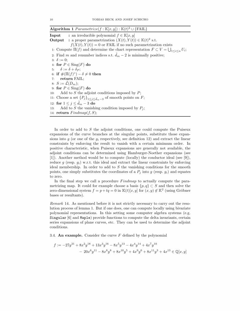
10 TOBIAS BECK AND JOSEF SCHICHO
Algorithm 1 Parametrize(f : K[x, y]) : K(t)2 ∪ {FAIL}Input : an irreducible polynomial f ∈ K[x, y]Output : a proper parametrization (X(t), Y (t)) ∈ K(t)2 s.t.
f(X(t), Y (t)) = 0 or FAIL if no such parametrization exists1: Compute Π(f) and determine the chart representation F ⊂ V =
⋃1≤i≤n Ui;
2: Find m and renumber indices s.t. dm − 2 is minimally positive;3: δ := 0;4: for P ∈ Sing(F ) do5: δ := δ + δP ;6: if #(Π(f)◦)− δ 6= 0 then7: return FAIL;8: S := L(Dm);9: for P ∈ Sing(F ) do
10: Add to S the adjoint conditions imposed by P ;11: Choose a set {Pj}1≤j≤dm−3 of smooth points on F ;
12: for 1 ≤ j ≤ dm − 3 do13: Add to S the vanishing condition imposed by Pj ;14: return Findmap(f, S);
In order to add to S the adjoint conditions, one could compute the Puiseuxexpansions of the curve branches at the singular points, substitute those expan-sions into g (or one of the gi respectively, see definition 12) and extract the linearconstraints by enforcing the result to vanish with a certain minimum order. Inpositive characteristic, when Puiseux expansions are generally not available, theadjoint conditions can be determined using Hamburger-Noether expansions (see[1]). Another method would be to compute (locally) the conductor ideal (see [9]),reduce g (resp. gi) w.r.t. this ideal and extract the linear constraints by enforcingideal membership. In order to add to S the vanishing conditions for the smoothpoints, one simply substitutes the coordinates of a Pj into g (resp. gi) and equatesto zero.
In the final step we call a procedure Findmap to actually compute the para-metrizing map. It could for example choose a basis {p, q} ⊂ S and then solve thezero-dimensional system f = p+ tq = 0 in K(t)[x, y] for (x, y) 6∈ K2 (using Grobnerbases or resultants).
Remark 14. As mentioned before it is not strictly necessary to carry out the reso-lution process of lemma 1. But if one does, one can compute locally using bivariatepolynomial representations. In this setting some computer algebra systems (e.g.Singular [6] and Maple) provide functions to compute the delta invariants, certainseries expansions of plane curves, etc. They can be used to determine the adjointconditions.
3.4. An example. Consider the curve F defined by the polynomial
f := −27y21 + 8x2y18 + 13x3y16 − 8x5y13 − 4x4y14 + 4x7y10
− 20x6y11 − 8x8y8 + 8x10y5 + 4x9y6 + 8x11y3 + 4x13 ∈ Q[x, y]
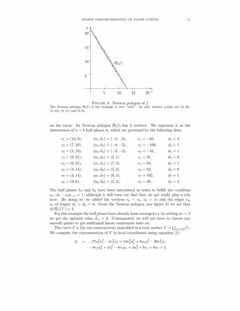
SPARSE PARAMETRIZATION OF PLANE CURVES 11
s
5 10 15 20
5
10
15
20
Π(f)
r
Figure 3. Newton polygon of fThe Newton polygon Π(f) of the example is very “slim”. Its only interior points are (3, 16),(5, 13), (6, 11) and (8, 8).
on the torus. Its Newton polygon Π(f) has 6 vertices. We represent it as theintersection of n = 8 half planes hi which are governed by the following data:
v1 = (13, 0), (a1, b1) = (−5,−3), c1 = −65, d1 = 2
v2 = (7, 10), (a2, b2) = (−8,−5), c2 = −106, d2 = 1
v3 = (2, 18), (a3, b3) = (−3,−2), c3 = −42, d3 = 1
v4 = (0, 21), (a4, b4) = (2, 1), c4 = 21, d4 = 0
v5 = (0, 21), (a5, b5) = (7, 4), c5 = 84, d5 = 1
v6 = (4, 14), (a6, b6) = (5, 3), c6 = 62, d6 = 0
v7 = (4, 14), (a7, b7) = (8, 5), c7 = 102, d7 = 1
v8 = (9, 6), (a8, b8) = (3, 2), c8 = 39, d8 = 2
The half planes h4 and h6 have been introduced in order to fulfill the conditionai−1bi − aibi−1 = 1, although it will turn out that they do not really play a rolehere. By doing so, we added the vertices v4 = v5, v6 = v7 and the edges e4,e6 of length d4 = d6 = 0. From the Newton polygon (see figure 3) we see that#(Π(f)◦) = 4.
For this example the half planes have already been arranged s.t. by settingm := 2we get the optimal value dm = 3. Consequently we will not have to choose anysmooth points to get additional linear constraints later on.
The curve F is (by our construction) embedded in a toric surface V =⋃
1≤i≤8 Ui.
We compute the representation of F in local coordinates using equation (1):
f1 = −27v21u
31 − 4v3
1u1 + 13v21u
21 + 8v1u
31 − 20v2
1u1
− 8v1u21 + 4v2
1 − 8v1u1 + 4u21 + 8v1 + 8u1 + 4
12 TOBIAS BECK AND JOSEF SCHICHO
f2 = −4v42u
32 + 4v4
2u22 − 20v3
2u22 + 8v3
2u2 + 13v22u
22
− 8v22u2 − 27v2u
22 + 4v2
2 − 8v2u2 + 8v2 + 8u2 + 4
f3 = 4v33u
43 + 8v3
3u33 − 4v2
3u43 + 4v3
3u23 − 20v2
3u33
− 8v23u
23 + 8v2
3u3 + 13v3u23 − 8v3u3 + 4v3 − 27u3 + 8
f4 = 4v54u
34 + 8v4
4u34 + 8v4
4u24 + 4v3
4u34 − 8v3
4u24
+ 4v34u4 − 20v2
4u24 − 8v2
4u4 − 4v4u24 + 13v4u4 + 8v4 − 27
f5 = 4v75u
55 + 8v6
5u45 + 8v5
5u45 + 4v5
5u35 − 8v4
5u35
+ 4v35u
35 − 8v3
5u25 − 20v2
5u25 + 8v2
5u5 + 13v5u5 − 4u5 − 27
f6 = 4v36u
76 + 8v3
6u66 + 4v3
6u56 + 8v2
6u56 − 8v2
6u46
− 8v26u
36 + 8v2
6u26 + 4v6u
36 − 20v6u
26 + 13v6u6 − 27v6 − 4
f7 = 4v47u
37 + 8v4
7u27 + 8v3
7u37 − 8v3
7u27 + 4v2
7u37
− 27v37u7 − 8v2
7u27 + 13v2
7u7 + 8v7u2 − 20v7u7 + 4u7 − 4
f8 = 8v38u
48 − 27v3
8u38 + 4v2
8u48 − 8v2
8u38 + 13v2
8u28
+ 8v8u38 − 8v8u
28 − 20v8u8 + 4u2
8 − 4v8 + 8u8 + 4
It turns out that F has a singular point P on the toric invariant divisor E1. Itshows up in the open subsets U1 and U2 and has coordinates (u1, v1) = (−1, 0),(u2, v2) = (0,−1) respectively. Another singular point Q ∈ E8 is lying in U1 andU8 with coordinates (u1, v1) = (0,−1) and (u8, v8) = (−1, 0). The curves F ∩Ui fori ∈ {3, 4, 5, 6, 7} are smooth. Hence all the information on the singularities can begathered in U1. For this purpose we compute the Puiseux expansions at the pointsP and Q:
σP (α) = − 14 (u1 + 1) + α(u1 + 1)2 + ( 435
608α− 512432 )(u1 + 1)3 . . .
σQ(α) = −1− 52u1 + βu2
1 + ( 214 β + 195
16 )u31 . . .
Here α denotes a root of 1024α2+516α+63 and β denotes a root of 16β2+24β−45.Taking conjugates into account we have two curve branches through each of thesingular points.
From these expansions one can compute amongst others the δ-invariants δP =δQ = 2 (for details we refer to [13]). We compute the genus g(F ) = #(Π(f)◦) −δP − δQ = 4− 2− 2 = 0, i.e. the curve F is indeed parametrizable.
Now we make an indetermined Ansatz for a polynomial in L(Dm). The supportof such a polynomial has to lie within Π(f) but not on the edges ei for i ∈ {3, . . . , 8}.
g := c1x3y16 + c2x
5y13 + c3x7y10 + c4x
6y11 + c5x8y8 + c6x
10y5
For obvious reasons, we only have to compute the local representation in U1 (seedefinition 12):
g1 = c1v21u1 + c4v
21 + c2v1u1 + c5v1 + c3u1 + c6
In order to be adjoint g1(σP ) has to vanish with order at least 2 around u1 = −1and g1(σQ) has to vanish with order at least 2 around u1 = 0 (again see [13]).Executing the substitutions and equating lowest terms to 0 one gets the linearconstraints 1
4c2 + c3 − 14c5 = 0, −c3 − c6 = 0 (from P ) and c4 − c5 + c6 = 0,
c1 − c2 + c3 + 5c4 − 52c5 = 0 (from Q). We solve this system w.r.t. parameters c3,
c4 and substitute the result into g to get a polynomial g ∈ Am (for any concrete
SPARSE PARAMETRIZATION OF PLANE CURVES 13
value of c3 and c4).
g = (− 32x
3y16 − 3x5y13 + x7y10 + x8y8 + x10y5)c3
+ (− 32x
3y16 + x5y13 + x6y11 + x8y8)c4
As a final step we solve the system {f = 0, g = 0, c3 = 1, c4 = t} for x and y inQ(t). It has two distinct solutions. One is (x, y) = (0, 0) which corresponds to thetwo singular points P and Q, the other one yields the parametrization:
X(t) =−256(2t2 + 4t− 1)3(t+ 1)7t8
(−1 + 8t)3(2t2 + 7t− 1)5
Y (t) =−32t5(2t2 + 4t− 1)2(t+ 1)4
(−1 + 8t)2(2t2 + 7t− 1)3
For illustrative purposes assume we had chosen m := 3 non-optimal (or we were
in a situation where a choice s.t. dm = 3 is not possible). We would get the following
indetermined Ansatz for a polynomial in L(Dm):
g := c0x2y18 + c1x
3y16 + c2x5y13 + c3x
7y10 + c4x6y11 + c5x
8y8 + c6x10y5
We compute the local representations in U1 and U5.
g1 = c1v21u1 + c0v1u
21 + c4v
21 + c2v1u1 + c5v1 + c3u1 + c6
g5 = c6v55u
35 + c3v
45u
25 + c5v
35u
25 + c2v
25u5 + c4v5u5 + c0v5 + c1
Proceeding as before, i.e. substituting the Puiseux expansions at the singular pointsP and Q in U1 into g1 we get the linear constraints − 1
4c0 + 14c2 + c3 − 1
4c5 = 0,
−c3 + c6 = 0, c4 − c5 + c6 = 0 and c1 − c2 + c3 + 5c4 − 52c5 = 0. Now we have to
choose an additional smooth point on F , e.g. (u5, v5) = (− 274 , 0) in U5. Plugging
these coordinates into g5 and equating the result to zero we get c1 = 0. We againsolve the system and substitute into g.
g = (−4x5y13 − x6y11 + x7y10 + x10y5)c6
+ (x2y18 + 53x
5y13 + 23x
6y11 + 23x
8y8)c0
Now in the same way as above we arrive at the following parametrization:
X(t) =(135− 108t+ 20t2)3(14t− 27)7(−3 + 2t)8
429981696(16t2− 18t− 27)5(t− 2)8t3
Y (t) =−(135− 108t+ 20t2)2(14t− 27)4(−3 + 2t)5
248832t2(16t2 − 18t− 27)3(t− 2)5
Remark 15. A conventional algorithm based on an embedding of the curve in theprojective plane P2
Q has to work very hard on that example. The correspondingcomplete curve would have again two singular points, but now the δ-invariants are119 and 71. These complicated singularities show up only because the structure ofthe Newton polygon is not taken into account. Proceeding in this setting like wedid, the involved linear systems are found as subspaces of a vector space of dimen-sion greater than 200. The excellent Maple implementation of a parametrizationalgorithm produced around 40 DIN A4 pages of output. (Of course we admit thatthe chosen example is especially well-fit for our method.)
14 TOBIAS BECK AND JOSEF SCHICHO
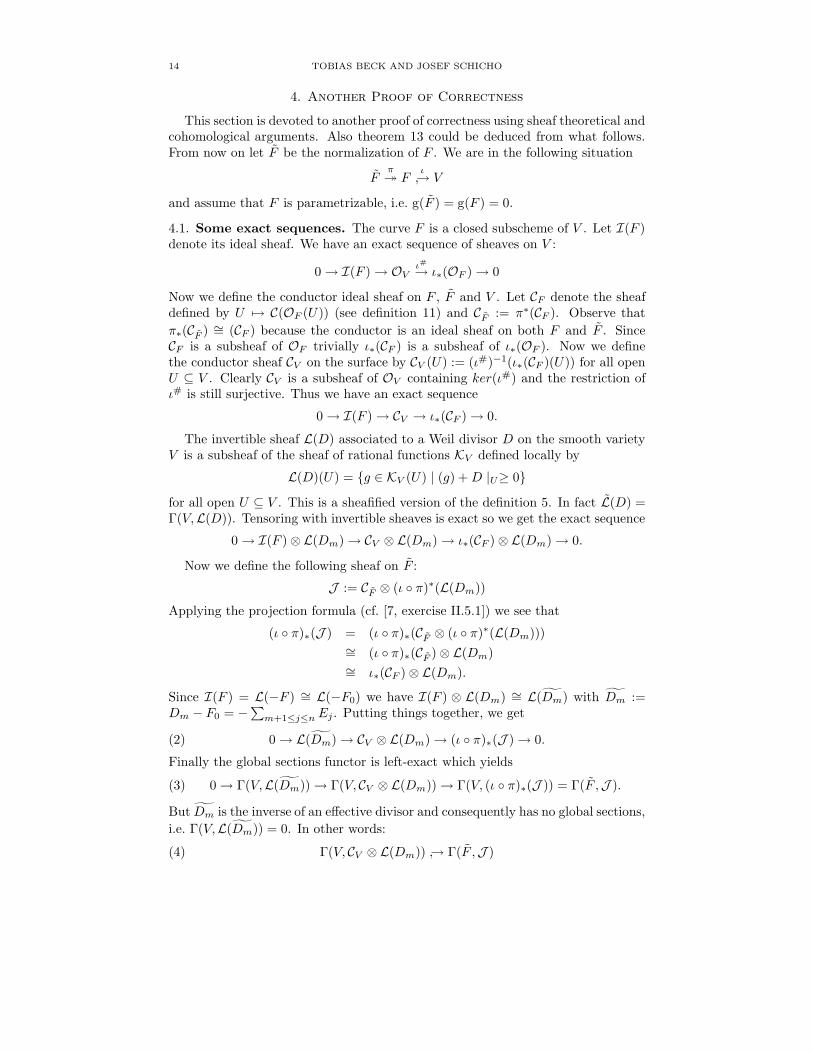
4. Another Proof of Correctness
This section is devoted to another proof of correctness using sheaf theoretical andcohomological arguments. Also theorem 13 could be deduced from what follows.From now on let F be the normalization of F . We are in the following situation
Fπ� F
ι↪→ V
and assume that F is parametrizable, i.e. g(F ) = g(F ) = 0.
4.1. Some exact sequences. The curve F is a closed subscheme of V . Let I(F )denote its ideal sheaf. We have an exact sequence of sheaves on V :
0→ I(F )→ OV ι#→ ι∗(OF )→ 0
Now we define the conductor ideal sheaf on F , F and V . Let CF denote the sheafdefined by U 7→ C(OF (U)) (see definition 11) and CF := π∗(CF ). Observe that
π∗(CF ) ∼= (CF ) because the conductor is an ideal sheaf on both F and F . SinceCF is a subsheaf of OF trivially ι∗(CF ) is a subsheaf of ι∗(OF ). Now we definethe conductor sheaf CV on the surface by CV (U) := (ι#)−1(ι∗(CF )(U)) for all openU ⊆ V . Clearly CV is a subsheaf of OV containing ker(ι#) and the restriction ofι# is still surjective. Thus we have an exact sequence
0→ I(F )→ CV → ι∗(CF )→ 0.
The invertible sheaf L(D) associated to a Weil divisor D on the smooth varietyV is a subsheaf of the sheaf of rational functions KV defined locally by
L(D)(U) = {g ∈ KV (U) | (g) +D |U≥ 0}for all open U ⊆ V . This is a sheafified version of the definition 5. In fact L(D) =Γ(V,L(D)). Tensoring with invertible sheaves is exact so we get the exact sequence
0→ I(F )⊗L(Dm)→ CV ⊗L(Dm)→ ι∗(CF )⊗L(Dm)→ 0.
Now we define the following sheaf on F :
J := CF ⊗ (ι ◦ π)∗(L(Dm))
Applying the projection formula (cf. [7, exercise II.5.1]) we see that
(ι ◦ π)∗(J ) = (ι ◦ π)∗(CF ⊗ (ι ◦ π)∗(L(Dm)))∼= (ι ◦ π)∗(CF )⊗L(Dm)∼= ι∗(CF )⊗L(Dm).
Since I(F ) = L(−F ) ∼= L(−F0) we have I(F ) ⊗ L(Dm) ∼= L(Dm) with Dm :=Dm − F0 = −∑m+1≤j≤n Ej . Putting things together, we get
0→ L(Dm)→ CV ⊗L(Dm)→ (ι ◦ π)∗(J )→ 0.(2)
Finally the global sections functor is left-exact which yields
0→ Γ(V,L(Dm))→ Γ(V, CV ⊗L(Dm))→ Γ(V, (ι ◦ π)∗(J )) = Γ(F ,J ).(3)
But Dm is the inverse of an effective divisor and consequently has no global sections,
i.e. Γ(V,L(Dm)) = 0. In other words:
Γ(V, CV ⊗L(Dm)) ↪→ Γ(F ,J )(4)
SPARSE PARAMETRIZATION OF PLANE CURVES 15
The global sections Γ(V, CV ⊗ L(Dm)) are very suitable for computation. Indeedif we write CV ⊗ L(Dm) as a sheaf of rational functions, we see that its globalsections correspond exactly to the system Am of definition 12. In fact the last mapof sequence (3) is also surjective and thus (4) is an isomorphism. We postpone thecohomological proof of this statement to the last section. Instead we proceed nowwith a brief study of the sheaf J and interpret the isomorphism in the context ofthe parametrization problem.
4.2. The sheaf on the normalized curve. First we reinterpret lemma 9 in thecontext of sheaves. In general for any divisor D ∈ Div(V ) it is true that deg((ι ◦π)∗(L(D))) = F ·D. Then F ·Dm = F0 ·Dm implies the following corollary.
Corollary 16. deg((ι ◦ π)∗(L(Dm))) = 2#(Π(f)◦) + dm − 2.
Proposition 17. If∑
1≤j≤m dj ≥ 2 then deg(J ) = dm − 2.
Proof. We compute the degree of J using deg(CF ) = −2∑P∈F δP (cf. [5]), corollary
16 and applying the genus formula of proposition 7:
deg(J ) = deg(CF ⊗ (ι ◦ π)∗(L(Dm)))= deg(CF ) + deg((ι ◦ π)∗(L(Dm)))
= −2∑P∈F δP + 2#(Γ(f)◦) + dm − 2
= 2(#(Γ(f)◦)−∑P∈F δP
)+ dm − 2
= dm − 2. �
Assume dm ≥ 3 and let d := dm − 2. Since F is assumed parametrizable, itsnormalization F is isomorphic to P1
K. Assume we have homogeneous coordinatesu, v on P1
K. Let P ∈ Div(P1K) be the prime divisor corresponding to u = 0. Any
invertible sheaf of degree d on P1K is isomorphic to L(dP ). This sheaf is generated by
its global sections Γ(P1K,L(dP )) = 〈vd/ud, vd−1u/ud, . . . , ud/ud〉. They constitute
a closed immersion ψ : P1K → PdK : [u : v] 7→ [vd : vd−1u : · · · : ud]. In other words,
a basis of the global section space Γ(F ,J ) defines an isomorphism between F andthe rational normal curve in PdK.
Remark 18. From this one could also get a slightly different proof of theorem 13because deg(J ) corresponds to the number of free intersections. The result on thedimension follows from the above arguments because dimK(Am) = dimK(Γ(V, CV ⊗L(Dm))) = dim(Γ(F ,J )) = deg(J ) + 1.
4.3. Reduction of the parametrization problem to rational normal curves.Write CV ⊗ L(Dm) as a sheaf of rational functions and identify J with L(dP ) onP1K as above. The functions in Γ(V, CV ⊗L(Dm)) do not have a pole along F . The
reader may check that isomorphism (4) is in fact given by the pullback (ι ◦ π)∗ ofrational functions.
Now let {s0, . . . , sd} ⊂ Γ(V, CV ⊗L(Dm))) be a basis s.t. (ι◦π)∗(si) = vd−iui/ud
and define a rational map by
φ : T → PdK : (x, y) 7→ [s0 : s1 : · · · : sd]

16 TOBIAS BECK AND JOSEF SCHICHO
on the torus. We find that it maps F (and hence also F ) birationally to the rationalnormal curve in PdK:
F ∼= P1Kι ◦ π- V
PdK
φ
?
ψ-
In the algorithm we finally choose a set of dm − 3 = d − 1 smooth points andrestrict the linear system using vanishing conditions imposed by these points. Inour current setting this corresponds to choosing points on the rational normal curveand projecting until we reach the projective line P1
K; the natural way to parametrizea rational normal curve.
4.4. Vanishing of the first cohomology. It remains to show that the last mapof sequence (3) is surjective. We will use Cech cohomology w.r.t. the natural affinecover U := {Ui}1≤i≤n to derive the desired result. From the short exact sequence(2) we get a long exact sequence
0 → Γ(V,L(Dm)) → Γ(V, CV ⊗L(Dm)) → Γ(V, (ι ◦ π)∗(J ))
→ H1(U,L(Dm)) → . . .
So we have to show that H1(U,L(Dm)) = 0.
To define Cech cohomology we use the following set of half planes:
hi := {(r, s) ∈ R2 | air + bis ≥ ∆i} where ∆i =
{0 for 1 ≤ i ≤ m and1 else
Using the coordinate transformations of section 2 and these half planes one describes
the needed sections of L(Dm) as K-vector spaces:
Γ(Ui,L(Dm)) = 〈xrys〉(r,s)∈hi−1∩hi for 1 ≤ i ≤ n,Γ(Ui−1 ∩ Ui,L(Dm)) = 〈xrys〉(r,s)∈hi for 2 ≤ i ≤ n,
Γ(Ui ∩ Uj ,L(Dm)) = 〈xrys〉(r,s)∈Z2 for 1 ≤ i < j ≤ n and j − i ≥ 2,
Γ(Ui ∩ Uj ∩ Uk,L(Dm)) = 〈xrys〉(r,s)∈Z2 for 1 ≤ i < j < k ≤ nThe first objects in the Cech complex are given by
C0(U,L(Dm)) =∏
1≤i≤nΓ(Ui,L(Dm)),
C1(U,L(Dm)) =∏
1≤i<j≤nΓ(Ui ∩ Uj ,L(Dm)),
C2(U,L(Dm)) =∏
1≤i<j<k≤nΓ(Ui ∩ Uj ∩ Uk,L(Dm))
and the first maps by
d0 : (gi)i 7→ (gj − gi)i<j ,d1 : (gi,j)i<j 7→ (gj,k − gi,k + gj,k)i<j<k .
SPARSE PARAMETRIZATION OF PLANE CURVES 17
r
s
4
3 7
2 1
65
r
s
h1
4
3 7
2 1
65
h5
(r, s)(r, s)
h1
h3
h3
h2
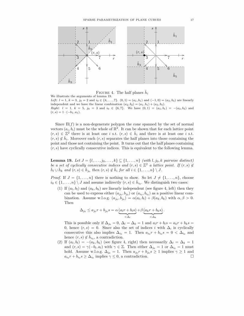
Figure 4. The half planes hiWe illustrate the arguments of lemma 19.Left: l = 1, k = 3, j0 = 2 and i0 ∈ {4, . . . , 7}. (0, 1) = (a1 , b1) and (−1, 0) = (a3 , b3) are linearlyindependent and we have the linear combination (a2, b2) = (a1 , b1) + (a3 , b3).Right: l = 1, k = 5, j0 = 3 and i0 ∈ {6, 7}. We have (0, 1) = (a1 , b1) = −(a3, b3) and(r, s) = 1 · (−b1, a1).
Since Π(f) is a non-degenerate polygon the cone spanned by the set of normalvectors (ai, bi) must be the whole of R2. It can be shown that for each lattice point(r, s) ∈ Z2 there is at least one i s.t. (r, s) ∈ hi and there is at least one i s.t.(r, s) 6∈ hi. Moreover each (r, s) separates the half planes into those containing thepoint and those not containing the point. It turns out that the half planes containing(r, s) have cyclically consecutive indices. This is equivalent to the following lemma.
Lemma 19. Let J = {l, . . . , j0, . . . , k} ⊆ {1, . . . , n} (with l, j0, k pairwise distinct)be a set of cyclically consecutive indices and (r, s) ∈ Z2 a lattice point. If (r, s) 6∈hl ∪ hk and (r, s) ∈ hj0 then (r, s) 6∈ hi for all i ∈ {1, . . . , n} \ J .
Proof. If J = {1, . . . , n} there is nothing to show. So let J 6= {1, . . . , n}, choosei0 ∈ {1, . . . , n} \ J and assume indirectly (r, s) ∈ hi0 . We distinguish two cases:
(1) If (al, bl) and (ak, bk) are linearly independent (see figure 4, left) then theycan be used to express either (aj0 , bj0) or (ai0 , bi0) as a positive linear com-bination. Assume w.l.o.g. (aj0 , bj0) = α(al, bl) + β(ak, bk) with α, β > 0.Then
∆j0 ≤ aj0r + bj0s = α (alr + bls)︸ ︷︷ ︸<∆l
+β (akr + bks)︸ ︷︷ ︸<∆k
.
This is possible only if ∆j0 = 0, ∆l = ∆k = 1 and alr + bls = akr + bks =0, hence (r, s) = 0. Since also the set of indices i with ∆i is cyclicallyconsecutive this also implies ∆i0 = 1. Then ai0r + bi0s = 0 < ∆i0 andhence (r, s) 6∈ hi0 , a contradiction.
(2) If (al, bl) = −(ak, bk) (see figure 4, right) then necessarily ∆l = ∆k = 1and (r, s) = γ(−bl, al) with γ ∈ Z. Then either ∆j0 = 1 or ∆i0 = 1 musthold. Assume w.l.o.g. ∆j0 = 1. Then aj0r + bj0s ≥ 1 implies γ ≥ 1 andai0r + bi0s ≥ ∆i0 implies γ ≤ 0, a contradiction. �
18 TOBIAS BECK AND JOSEF SCHICHO
For an element g = (gl,k)l<k ∈ ker(d1) we have gl,k = gl,i + gi,k for l < i < k.From this follows gl,k =
∑l<i≤k gi−1,i. Hence g is uniquely determined by gi−1,i
for 1 < i ≤ n. Writing g0,1 = gn,1 = −g1,n we get in particular∑
1≤i≤n gi−1,i = 0.
Because of the structure of the section spaces, we may describe C0, d0 etc. in anobvious way as direct sums with indices (r, s). We indicate this by subscripts, i.e.C0
(r,s), d0(r,s) etc.
Proposition 20. The first cohomology of L(Dm) vanishes: H1(U,L(Dm)) = 0.
Proof. We have to show im(d0) = ker(d1). For this we fix an arbitrary lattice point(r, s) ∈ Z2 and show im(d0
(r,s)) = ker(d1(r,s)). Let g ∈ ker(d1
(r,s)). Using lemma 19
we may assume w.l.o.g. that there is an l < n s.t. (r, s) ∈ hi for 1 ≤ i ≤ l but(r, s) 6∈ hi for l < i ≤ n.
We can find a d0(r,s)-preimage of g by setting g1 := 0, gi := gi−1 + gi−1,i for
1 < i ≤ l and gi := 0 for l < i ≤ n. First observe that with this definition we really
have (gi)i ∈ C0(r,s)(U,L(Dm)) because gi 6= 0 implies (r, s) ∈ hi−1 ∩ hi.
Now we check that g = d0(r,s)((gi)i): For 1 < i ≤ l we get gi−1,i = gi − gi−1
by definition. For l + 1 < i ≤ n we know that (r, s) 6∈ hi−1 and (r, s) 6∈ hi, i.e.gi−1,i = gi = gi−1 = 0, hence again gi−1,i = gi − gi−1. This also implies
0 =∑
1≤i≤n gi−1,i =∑
1<i≤l+1 gi−1,i =(∑
1<i≤l gi − gi−1
)+ gl,l+1 = gl + gl,l+1
or equivalently gl,l+1 = 0− gl = gl+1 − gl. �
5. Conclusion
We presented a method for the rational parametrization of plane algebraic curves(on the torus). The main idea was to embed the curve in a toric surface that isadapted to the shape of the Newton polygon. We showed one possible methodto parametrize in this setting. But also other algorithms like [14] and [8] couldpossibly benefit from this approach.
Up to now sparsity of the defining equation is used as far as the Newton polygonis considerably smaller than a full triangle. Another sort of sparsity would be whenthe lattice spanned by the support of the equation is not the whole of Z2 but onlya sublattice. We also think about studying that case.
In this article we have assumed an algebraically closed coefficient field. We havenot taken into account the degree of the field extension needed to represent theparametrization when starting from a non-closed field. This has been addressed forexample in [11]. The ideas should carry over to our situation. Parametrization ofrational normal curves using a field extension of least possible degree can also beachieved using the Lie algebra method in [3].
References
[1] A. Campillo and J. I. Farran. Symbolic Hamburger-Noether expressions of plane curves andapplications to AG codes. Math. Comp., 71(240):1759–1780 (electronic), 2002.
[2] David Cox. What is a toric variety? In Topics in Algebraic Geometry and Geometric Mod-eling, volume 334 of Contemporary Mathematics, pages 203–223. American MathematicalSociety, Providence, Rhode Island, 2003. Workshop on Algebraic Geometry and GeometricModeling (Vilnius, 2002).
SPARSE PARAMETRIZATION OF PLANE CURVES 19
[3] Willem A. de Graaf, Michael Harrison, Jana Pilnikova, and Josef Schicho. A Lie AlgebraMethod for Rational Parametrization of Severi-Brauer Surfaces. 2005. submitted for publica-tion and electronically available at http://arxiv.org/abs/math.AG/0501157.
[4] William Fulton. Introduction to toric varieties, volume 131 of Annals of Mathematics Stud-ies. Princeton University Press, Princeton, NJ, 1993. The William H. Roever Lectures inGeometry.
[5] Daniel Gorenstein. An arithmetic theory of adjoint plane curves. Trans. Amer. Math. Soc.,72:414–436, 1952.
[6] G.-M. Greuel, G. Pfister, and H. Schonemann. Singular 2.0. A Computer Algebra Systemfor Polynomial Computations, Centre for Computer Algebra, University of Kaiserslautern,2001. http://www.singular.uni-kl.de.
[7] Robin Hartshorne. Algebraic geometry. Springer-Verlag, New York, 1977. Graduate Texts inMathematics, No. 52.
[8] F. Hess. Computing Riemann-Roch spaces in algebraic function fields and related topics. J.Symbolic Comput., 33(4):425–445, 2002.
[9] Michal Mnuk. An algebraic approach to computing adjoint curves. J. Symbolic Comput., 23(2-3):229–240, 1997. Parametric algebraic curves and applications (Albuquerque, NM, 1995).
[10] J. Rafael Sendra and Franz Winkler. Symbolic parametrization of curves. J. Symbolic Com-put., 12(6):607–631, 1991.
[11] J. Rafael Sendra and Franz Winkler. Parametrization of algebraic curves over optimal fieldextensions. J. Symbolic Comput., 23(2-3):191–207, 1997. Parametric algebraic curves andapplications (Albuquerque, NM, 1995).
[12] Igor R. Shafarevich. Basic algebraic geometry. 1. Springer-Verlag, Berlin, second edition,1994. Varieties in projective space, Translated from the 1988 Russian edition and with notesby Miles Reid.
[13] Peter Stadelmeyer. On the Computational Complexity of Resolving Curve Singularities andRelated Problems. Technical Report 00-31, RISC-Linz, A-4232 Hagenberg, December 2000.PhD Thesis.
[14] Mark van Hoeij. Rational parametrizations of algebraic curves using a canonical divisor.J. Symbolic Comput., 23(2-3):209–227, 1997. Parametric algebraic curves and applications(Albuquerque, NM, 1995).
[15] Oscar Zariski and Pierre Samuel. Commutative algebra. Vol. I. Springer-Verlag, New York,1975. With the cooperation of I. S. Cohen, Corrected reprinting of the 1958 edition, GraduateTexts in Mathematics, No. 28.
Johann Radon Institute for Computational and Applied Mathematics, Altenberger-
straße 69, A–4040 Linz, Austrian Academy of Sciences